Embed Size (px)
Citation preview

Refinements in HierarchicalPhrase-Based
Translation Systems
Juan Miguel Pino
Cambridge University Engineering Department
Dissertation submitted to the University of Cambridge for the degree ofDoctor of Philosophy

Declaration
I hereby declare that the contents of this dissertation are original and havenot been submitted in whole or in part for consideration for any other degreeor qualification in this, or any other University. This dissertation is the resultof my own work and includes nothing which is the outcome of work done incollaboration, except where specifically indicated in the text. This disser-tation contains less than 65,000 words including appendices, bibliography,footnotes, tables and equations and has less than 150 figures.
i

Acknowledgements
First, I am truly indebted to my supervisor Prof. Bill Byrne. Bill providedrelentless support throughout my PhD studies. He taught me how to bea better writer and a better researcher. I am also very grateful that heprovided me with invaluable opportunities such as participating in translationcompetitions or carrying out an internship at Google for three months.
I also would like to thank Dr. Stephen Clark and Dr. Miles Osborne forbeing part of my thesis committee and providing very valuable feedback onthe first submission of this thesis.
Without the lab Computer Officers, Patrick Gosling and Anna Langley,experiments reported in this thesis would not have been possible, I am there-fore grateful for all their hard work on the computer systems.
I also wish to thank all my colleagues at the Machine Intelligence Lab. Dr.Adria de Gispert provided me with critical guidance throughout my research:two chapters of this thesis originated from a very fruitful collaboration withhim. I am grateful to Aurelien Waite for all his help on infrastructure andfor helping me becoming a better engineer. Thanks to Dr. Gonzalo Iglesiasfor illuminating discussions on FSTs for machine translation as well as C++software engineering. Dr. Graeme Blackwood and Dr. Jamie Brunning pro-vided much support at the start of my studies as well as critical translationtools such as word alignment and lattice rescoring tools.
I am also in debt to my office colleagues Matt Shannon, Matt Seigel andChao Zhang for making PhD studies a pleasurable experience.
Finally, thank you Anna for your infinite patience, guidance and supportand for telling me to apply for at least two jobs at the end of my studies.Thank you Sofia and Fania: I will try to teach you many languages, just incase machine translation doesn’t improve quickly enough.
ii

Abstract
The relatively recently proposed hierarchical phrase-based translation modelfor statistical machine translation (SMT) has achieved state-of-the-art per-formance in numerous recent translation evaluations. Hierarchical phrase-based systems comprise a pipeline of modules with complex interactions. Inthis thesis, we propose refinements to the hierarchical phrase-based modelas well as improvements and analyses in various modules for hierarchicalphrase-based systems.
We took the opportunity of increasing amounts of available training datafor machine translation as well as existing frameworks for distributed com-puting in order to build better infrastructure for extraction, estimation andretrieval of hierarchical phrase-based grammars. We design and implementgrammar extraction as a series of Hadoop MapReduce jobs. We store the re-sulting grammar using the HFile format, which offers competitive trade-offsin terms of efficiency and simplicity. We demonstrate improvements over twoalternative solutions used in machine translation.
The modular nature of the SMT pipeline, while allowing individual im-provements, has the disadvantage that errors committed by one module arepropagated to the next. This thesis alleviates this issue between the wordalignment module and the grammar extraction and estimation module byconsidering richer statistics from word alignment models in extraction. Weuse alignment link and alignment phrase pair posterior probabilities for gram-mar extraction and estimation and demonstrate translation improvements inChinese to English translation.
This thesis also proposes refinements in grammar and language modellingboth in the context of domain adaptation and in the context of the interactionbetween first-pass decoding and lattice rescoring. We analyse alternativestrategies for grammar and language model cross-domain adaptation. Wealso study interactions between first-pass and second-pass language model in
iii

iv
terms of size and n-gram order. Finally, we analyse two smoothing methodsfor large 5-gram language model rescoring.
The last two chapters are devoted to the application of phrase-basedgrammars to the string regeneration task, which we consider as a means tostudy the fluency of machine translation output. We design and implement amonolingual phrase-based decoder for string regeneration and achieve state-of-the-art performance on this task. By applying our decoder to the outputof a hierarchical phrase-based translation system, we are able to recover thesame level of translation quality as the translation system.

Contents
1 Introduction 11.1 Machine translation . . . . . . . . . . . . . . . . . . . . . . . . 1
1.1.1 Challenges for Translation . . . . . . . . . . . . . . . . 11.1.2 Machine Translation Current Quality . . . . . . . . . . 2
1.2 Statistical Machine Translation . . . . . . . . . . . . . . . . . 51.2.1 The SMT Pipeline . . . . . . . . . . . . . . . . . . . . 5
1.3 Contributions . . . . . . . . . . . . . . . . . . . . . . . . . . . 61.4 Organisation of the thesis . . . . . . . . . . . . . . . . . . . . 8
2 Statistical Machine Translation 92.1 Historical Background . . . . . . . . . . . . . . . . . . . . . . 102.2 Source-Channel Model . . . . . . . . . . . . . . . . . . . . . . 102.3 Word Alignment . . . . . . . . . . . . . . . . . . . . . . . . . 12
2.3.1 HMM and Word-to-Phrase Alignment Models . . . . . 142.3.2 Symmetrisation Heuristics . . . . . . . . . . . . . . . . 16
2.4 Log-Linear Model of Machine Translation . . . . . . . . . . . . 192.5 Phrase-Based Translation . . . . . . . . . . . . . . . . . . . . 21
2.5.1 Alignment Template Model . . . . . . . . . . . . . . . 212.5.2 Phrase-Based Model . . . . . . . . . . . . . . . . . . . 222.5.3 Phrase Pair Extraction . . . . . . . . . . . . . . . . . . 222.5.4 Phrase-Based Decoding . . . . . . . . . . . . . . . . . . 24
2.6 Hierarchical Phrase-Based Translation . . . . . . . . . . . . . 262.6.1 Introduction and Motivation . . . . . . . . . . . . . . . 272.6.2 Hierarchical Grammar . . . . . . . . . . . . . . . . . . 272.6.3 Log-linear Model for Hierarchical Phrase-Based Trans-
lation . . . . . . . . . . . . . . . . . . . . . . . . . . . 332.6.4 Rule Extraction . . . . . . . . . . . . . . . . . . . . . . 352.6.5 Features . . . . . . . . . . . . . . . . . . . . . . . . . . 35
v
CONTENTS vi
2.7 Language Modelling . . . . . . . . . . . . . . . . . . . . . . . 362.7.1 n-gram language models . . . . . . . . . . . . . . . . . 372.7.2 Back-off and Interpolated Models . . . . . . . . . . . . 382.7.3 Modified Kneser-Ney Smoothing . . . . . . . . . . . . . 392.7.4 Stupid Backoff Smoothing . . . . . . . . . . . . . . . . 40
2.8 Optimisation . . . . . . . . . . . . . . . . . . . . . . . . . . . 402.8.1 Evaluation Metrics . . . . . . . . . . . . . . . . . . . . 402.8.2 Minimum Error Rate Training . . . . . . . . . . . . . . 42
2.9 Decoding with Finite State Transducers . . . . . . . . . . . . . 422.10 Lattice Rescoring . . . . . . . . . . . . . . . . . . . . . . . . . 43
2.10.1 5-gram Language Model Lattice Rescoring . . . . . . . 432.10.2 Lattice Minimum Bayes’ Risk Rescoring . . . . . . . . 442.10.3 Lattice Minimum Bayes-Risk for System Combination . 45
3 Data Structures for Hierarchical Phrase-Based TranslationGrammars 473.1 Introduction . . . . . . . . . . . . . . . . . . . . . . . . . . . . 483.2 Related Work . . . . . . . . . . . . . . . . . . . . . . . . . . . 50
3.2.1 Applications of MapReduce to SMT . . . . . . . . . . . 503.2.2 SMT Models Storage and Retrieval Solutions . . . . . . 52
3.3 HFile Description . . . . . . . . . . . . . . . . . . . . . . . . . 553.3.1 HFile Internal Structure . . . . . . . . . . . . . . . . . 553.3.2 Record Retrieval . . . . . . . . . . . . . . . . . . . . . 573.3.3 Bloom Filter Optimisation for Query Retrieval . . . . . 573.3.4 Local Disk Optimisation . . . . . . . . . . . . . . . . . 583.3.5 Query sorting optimisation . . . . . . . . . . . . . . . . 58
3.4 Hierarchical Rule Extraction with MapReduce . . . . . . . . . 583.4.1 Rule Extraction . . . . . . . . . . . . . . . . . . . . . . 593.4.2 Corpus-Level Feature Computation . . . . . . . . . . . 613.4.3 Feature Merging . . . . . . . . . . . . . . . . . . . . . 62
3.5 Hierarchical Rule Filtering for Translation . . . . . . . . . . . 623.5.1 Task Description . . . . . . . . . . . . . . . . . . . . . 633.5.2 HFile for Hierarchical Phrase-Based Grammars . . . . 633.5.3 Suffix Arrays for Hierarchical Phrase-Based Grammars 643.5.4 Text File Representation of Hierarchical Phrase-Based
Grammars . . . . . . . . . . . . . . . . . . . . . . . . . 643.5.5 Experimental Design . . . . . . . . . . . . . . . . . . . 653.5.6 Results and Discussion . . . . . . . . . . . . . . . . . . 67

CONTENTS vii
3.6 Conclusion . . . . . . . . . . . . . . . . . . . . . . . . . . . . . 70
4 Hierarchical Phrase-Based Grammar Extraction from Align-ment Posterior Probabilities 724.1 Introduction . . . . . . . . . . . . . . . . . . . . . . . . . . . . 734.2 Related Work . . . . . . . . . . . . . . . . . . . . . . . . . . . 744.3 Rule Extraction . . . . . . . . . . . . . . . . . . . . . . . . . . 77
4.3.1 General Framework for Rule Extraction . . . . . . . . . 784.3.2 Extraction from Viterbi Alignment Links . . . . . . . . 794.3.3 Extraction from Posteriors Probabilities over Align-
ment Links . . . . . . . . . . . . . . . . . . . . . . . . 814.3.4 Extraction from Posteriors over Phrase Pairs . . . . . . 874.3.5 Hierarchical Rule Extraction . . . . . . . . . . . . . . . 91
4.4 Experiments . . . . . . . . . . . . . . . . . . . . . . . . . . . . 964.4.1 Experimental Setup: Grammar Pattern Definition . . . 964.4.2 Experimental Setup . . . . . . . . . . . . . . . . . . . . 974.4.3 Grammar Coverage . . . . . . . . . . . . . . . . . . . . 994.4.4 Translation Results . . . . . . . . . . . . . . . . . . . . 1014.4.5 Comparison between WP and PP . . . . . . . . . . . 1044.4.6 Symmetrising Alignments of Parallel Text . . . . . . . 1044.4.7 Additional Language Pair: Russian-English . . . . . . . 106
4.5 Conclusion . . . . . . . . . . . . . . . . . . . . . . . . . . . . . 108
5 Domain Adaptation for Hierarchical Phrase-Based Transla-tion Systems 1095.1 Introduction . . . . . . . . . . . . . . . . . . . . . . . . . . . . 1095.2 Description of the System to be Developed . . . . . . . . . . . 1105.3 Domain Adaptation for Machine Translation . . . . . . . . . . 114
5.3.1 Domain Adaptation . . . . . . . . . . . . . . . . . . . . 1145.3.2 Previous Work on Domain Adaptation for SMT . . . . 115
5.4 Language Model Adaptation for Machine Translation . . . . . 1165.5 Domain Adaptation with Provenance Features . . . . . . . . . 1185.6 Interaction between First Pass Language Model and Rescoring
Language Model . . . . . . . . . . . . . . . . . . . . . . . . . . 1205.7 Language Model Smoothing in Language Model Lattice Rescor-
ing . . . . . . . . . . . . . . . . . . . . . . . . . . . . . . . . . 1225.8 Conclusion . . . . . . . . . . . . . . . . . . . . . . . . . . . . . 122

CONTENTS viii
6 String Regeneration as Phrase-Based Translation 1256.1 Introduction . . . . . . . . . . . . . . . . . . . . . . . . . . . . 1266.2 Background . . . . . . . . . . . . . . . . . . . . . . . . . . . . 1286.3 Phrase-Based Translation Model for String Regeneration . . . 1306.4 Phrase-Based Translation Rules for String Regeneration . . . . 131
6.4.1 Rule Extraction . . . . . . . . . . . . . . . . . . . . . . 1316.4.2 Rule Filtering . . . . . . . . . . . . . . . . . . . . . . . 132
6.5 String Regeneration Search . . . . . . . . . . . . . . . . . . . . 1326.5.1 Input . . . . . . . . . . . . . . . . . . . . . . . . . . . . 1336.5.2 Algorithm . . . . . . . . . . . . . . . . . . . . . . . . . 1336.5.3 FST Building . . . . . . . . . . . . . . . . . . . . . . . 1376.5.4 Example . . . . . . . . . . . . . . . . . . . . . . . . . . 137
6.6 Experiments . . . . . . . . . . . . . . . . . . . . . . . . . . . . 1396.6.1 Experimental Setup . . . . . . . . . . . . . . . . . . . . 1396.6.2 Baseline . . . . . . . . . . . . . . . . . . . . . . . . . . 1406.6.3 Sentence Splitting . . . . . . . . . . . . . . . . . . . . . 1406.6.4 Pruning . . . . . . . . . . . . . . . . . . . . . . . . . . 1416.6.5 n-gram Order for n-gram Rules . . . . . . . . . . . . . 1426.6.6 Overlapping n-gram Rules . . . . . . . . . . . . . . . . 1446.6.7 Future Cost . . . . . . . . . . . . . . . . . . . . . . . . 1456.6.8 Rescoring . . . . . . . . . . . . . . . . . . . . . . . . . 147
6.7 Conclusion . . . . . . . . . . . . . . . . . . . . . . . . . . . . . 148
7 String Regeneration Applied to Machine Translation 1507.1 SMT Baseline System . . . . . . . . . . . . . . . . . . . . . . 1517.2 Regeneration Decoder Baseline on MT Output . . . . . . . . . 1527.3 Analysis of the Loss of MT Hypotheses . . . . . . . . . . . . . 1547.4 Biased Language Model for Regeneration . . . . . . . . . . . . 1577.5 Translation and Regeneration Hypothesis Combination . . . . 1577.6 Conclusion . . . . . . . . . . . . . . . . . . . . . . . . . . . . . 160
8 Summary and Future Work 1618.1 Review of Work . . . . . . . . . . . . . . . . . . . . . . . . . . 161
8.1.1 Hierarchical Phrase-Based Grammars: Infrastructure . 1628.1.2 Hierarchical Phrase-Based Grammars: Modelling . . . 1628.1.3 Hierarchical Phrase-Based System Development . . . . 1638.1.4 Fluency in Hierarchical Phrase-Based Systems . . . . . 163
8.2 Future Work . . . . . . . . . . . . . . . . . . . . . . . . . . . . 164

Chapter 1
Introduction
1.1 Machine translationMachine translation is the process of translation from input speech or text ina natural language into another natural language by some kind of automaticsystem. Real world examples include online services such as Google Trans-late1, Bing Translate2, SDL3, PROMT4, etc. Interacting with any onlineautomatic translation service with the expectation of a high quality transla-tion can be a frustrating experience. Indeed, variations in word order acrosslanguages and syntax and the use of real world knowledge for puns or idiomsmake translation a very challenging task.
1.1.1 Challenges for Translation
In order to illustrate the difficulties that arise in translation, we present sev-eral examples that make translation challenging for humans, and a fortiorifor computers. In some languages, some concepts are common enough to bedesignated by one word, but in another language, an entire sentence may beneeded to describe that concept. For example, the word sobremesa in Span-ish can be translated into English as the time spent after a meal, talking tothe people with whom the meal was shared.5 In this situation, a human trans-
1 https://translate.google.com2 https://www.bing.com/translator3 http://www.freetranslation.com/4 http://www.online-translator.com5 http://blog.maptia.com/posts/untranslatable-words-from-other-cultures
1

CHAPTER 1. INTRODUCTION 2
lator is left with the choice of keeping the translation short but inexact orlong but cumbersome. For a computer, or rather a statistical model, such asituation will represent an outlier in terms of the ratio of the number of wordsthat are translation of each other. Self-referential sentences can also presentchallenges for translation. For example, the sentence This sentence has fivewords has at least two acceptable translations into Russian from the syntac-tic and semantic point of view: В этом предложении пять слов and Этопредложение состоит из пяти слов. However, the second translation hassix words and therefore cannot be accepted. Another challenge for transla-tion is word ordering. The first sentence of the novel The Metamorphosis byFranz Kafka reads Als Gregor Samsa eines Morgens aus unruhigen Traumenerwachte, fand er sich in seinem Bett zu einem ungeheuren Ungeziefer ver-wandelt. One possible English translation is As Gregor Samsa awoke onemorning from uneasy dreams, he found himself transformed in his bed intoa gigantic insect-like creature. In German, the words for transformed (ver-wandelt) and insect (Ungeziefer) come right at the end of the sentence andcreate an effect of surprise for the reader. In English, however, the verbtransformed comes in the middle of the sentence and the effect of surpriseis not as great. This example demonstrates how variations in word order-ing between languages can make translation challenging. Computers havethe additional challenge that the choice of word ordering should produce agrammatical sentence. This is a challenge for humans too but computers areparticularly bad at producing a grammatical output.
1.1.2 Machine Translation Current Quality
Even though machine translation is a challenging task, it is still useful ina number of situations. For example, machine translation can be used toobtain the gist, i.e. the general meaning, of a document in a foreign language.Machine translation can also be used for post-editing: a document in a foreignlanguage is first automatically translated and then the translation is correctedby a human translators. This is precisely the approach taken by translationcompanies such as Unbabel6.
Machine translation has therefore gotten to the point where it is actuallyuseful for practical applications, but it is reasonable to ask how far we arefrom perfect translation. We give indications in terms of the BLEU met-
6 https://www.unbabel.com

CHAPTER 1. INTRODUCTION 3
System 1-2-3-4 2-3-4 1-3-4 1-2-4 1-2-3CUED 38.95 34.80 35.60 35.87 35.28Reference 1 – 46.19 – – –Reference 2 – – 47.27 – –Reference 3 – – – 45.43 –Reference 4 – – – – 46.90
Table 1.1: BLEU score obtained by the Cambridge University EngineeringDepartment system and by human translators on the MT08 test set. 4 refer-ences are provided. The BLEU score is measured against various subsets ofreferences: all references (1-2-3-4), all but the first (2-3-4), etc. The BLEUscore for a human reference when the set of reference contains the humanreference is not computed and is simply 100.
ric (Papineni et al., 2002), which we will define in Section 2.8.1. For now, wesimply need to know that BLEU measures how well a translation hypothesisresembles a set of human translation references. The Cambridge Univer-sity Engineering Department (CUED) submitted a translation system to theNIST Open Machine Translation 2012 Evaluation.7 We run this system onthe newswire portion of the NIST Open Machine Translation 2008 Evalua-tion test set (MT08). For this MT08 test set, 4 references are available. Wemeasure the case insensitive BLEU score of the CUED system against the 4references and against subsets of 3 references. Similarly, we measure the caseinsensitive BLEU score of each reference against the other references. BLEUscores for humans and for the CUED system are summarised in Table 1.1.On average, CUED obtains a BLEU score of 35.39 against 3 references. Onaverage, human references obtain a BLEU score 46.45 against the other ref-erences. We can draw two conclusions from these observations. First, thisis evidence that many possible translations are acceptable. Second, becausethe automatic system performance for this particular setting is approximately10 BLEU points below human performance, this gives an indication of thequality of state-of-the-art automatic translation. After manual inspectionof the system output, we show a few examples of output sentences that arerelatively long and still have reasonable quality in Figure 1.1:
7 http://www.nist.gov/itl/iad/mig/openmt12.cfm

CHAPTER 1. INTRODUCTION 4
Minister of agriculture and social affairs, told AFP: “The primeminister submitted his resignation to Abbas, chairman of thepresident, and at the same time asked him to form a new cabinet,responsible for handling daily affairs of the new government.”
Reference: Minister for Agriculture and Social Affairs Habbashtold AFP: “Prime Minister Fayyad offered his resignation to Pres-ident Abbas. The president accepted it and at the same time alsoasked him to form a new cabinet government to be responsiblefor routine administration.”
Chavez has ordered government officials to keep an eye on foreign-ers visiting venezuela’s speech, when a person is found to havepublicly criticized him or the Venezuelan government, are to bedeported.
Reference: Chavez has already ordered government officialsto closely monitor the speech of foreigners when they visitVenezuela. If anyone is found publicly criticizing him or theVenezuelan government, they should be all deported.
US-China strategic economic dialogue “focused on the economic,environmental and other issues, the most important thing is thatthe issue of the RMB exchange rate, the US Congress membersare of the view that the value of the Renminbi underestimated.
Reference: The US-China Strategic Economic Dialogue mainlydiscusses economic, environmental protection and other issues.Yet, the most important is the issue of the renminbi exchangerate. US congressmen believe that the renminbi is excessivelyundervalued.
Figure 1.1: Example output of a translation system, together with one ref-erence. Even though the sentences are relatively long, they are overall fluentand intelligible. True casing is restored manually.
CHAPTER 1. INTRODUCTION 5
1.2 Statistical Machine TranslationThe current dominant approach to machine translation is a statistical ap-proach. Given an input in a natural language, a statistical model of trans-lation will attempt to predict the best translation according to a statisticalcriterion, such as the most likely translation under a probabilistic model oftranslation. The data used to estimate the parameters for such a modelconsists of a parallel corpus, which is a set of sentence pairs in two differ-ent natural languages that are translation of each other, and a monolingualcorpus which is a set of sentences in the language we would like to translateinto.
Parallel data can be obtained from multilingual institutions proceedingssuch as the United Nations (Franz et al., 2013),the Canadian Hansard (Ger-mann, 2001) or the European Parliament (Koehn, 2005). This type of datais relatively clean since it is created by professional translators. However, itmay not match the genre of the input sentences we wish to translate, suchas newswire. The importance of having a good match between the data usedfor training and testing is discussed in Section 5.3. In order to address thisconcern and also in order to obtain more data, parallel data can also beextracted automatically from comparable corpora (Smith et al., 2013). How-ever, the widespread availability of machine translation and the developmentof automatic techniques to extract parallel corpora automatically increasethe risk of having automatically translated output of poor quality present inthe training data. These concerns have been acknowledged and addressed bya watermarking algorithm (Venugopal et al., 2011).
1.2.1 The SMT Pipeline
Typically, state-of-the-art SMT systems are organised into a pipeline of de-terministic or statistical modules, as shown in Figure 1.2. Parallel text is firstpreprocessed. This consists of data cleaning and tokenisation. For morpho-logically poor languages such as English, simple rules for tokenisation, e.g.separate words by white space and punctuation, are usually good enough.For morphologically rich languages, more advanced techniques are neededfor effective tokenisation, for example morphological analysis (Habash andRambow, 2005), in order to combat data sparsity and work with a vocabu-lary with reasonable size. In the case of languages without word boundaries,such as Chinese, word segmentation techniques need to be applied (Zhang
CHAPTER 1. INTRODUCTION 6
and Clark, 2007), in order to be able to break sentences into words.The preprocessed parallel text is then word-aligned (see Section 2.3). A
word alignment is simply a mapping between source words and target wordsin a parallel sentence pair. Word alignment models were originally used todescribe the translation process and to perform translation (Germann et al.,2001). Word alignment toolkits are available online8,9 as well as a word toword translation decoder.10 Nowadays, word alignment models are used asan intermediate step in the translation pipeline. A translation grammar isthen extracted and estimated from the word alignments (see Section 2.6.4)and translation is performed under the translation grammar.
The monolingual data is also preprocessed in the same fashion as thetarget side of the parallel text and one or more language models are esti-mated from this data (see section Section 2.7). The language models andthe translation grammar are used by the translation decoder for translation.In order to optimise the SMT model parameters, alternating decoding andtuning steps are carried out.
Typically, a decoder can output a best possible translation, or an n-best list of translations or even a lattice of translations, which is a compactrepresentation of an n-best list with a very large number n. In the latter case,optional rescoring steps can be carried out in order to include models thatare too complex or not robust enough to be included in first pass decoding(see Section 2.10). In particular, we study a model of string regeneration thatallows any reordering of the output of the first pass decoder in Chapter 7.
1.3 ContributionsThe contributions of this thesis are outlined as follows:
• We describe a novel approach to grammar extraction and estimation.Our approach ties the models of word alignment and grammar extrac-tion and estimation more closely. It results in a more robust extractionand estimation of translation grammars and leads to improvements intranslation quality, as demonstrated in Chinese to English translationexperiments.
8 http://mi.eng.cam.ac.uk/~wjb31/distrib/mttkv19 https://code.google.com/p/giza-pp
10 http://www.isi.edu/licensed-sw/rewrite-decoder

CHAPTER 1. INTRODUCTION 7
..Parallel Text.
Preprocessing
.
Word Alignment
.
Grammar Extraction
. Monolingual Text.
Preprocessing
.
Language Modelling
..
Decoding
.
Tuning
.
Rescoring
Figure 1.2: Machine Translation System Development Pipeline

CHAPTER 1. INTRODUCTION 8
• We describe a system that allows the efficient extraction and filtering ofvery large grammars. This method has been in continued use at CUEDand was employed for submissions to the NIST 201211 and the WMT2013 (Bojar et al., 2013) translation evaluations. This was a carefullyengineering effort that required detailed understanding of grammar ex-traction procedures and how to implement them in a Hadoop frame-work. There are many implementation strategies that can be taken,but obtaining the processing performance needed to support the ex-periments reported in this thesis requires a careful design process.
• We designed and implemented a system for string regeneration, inspiredfrom phrase-based SMT techniques. We obtain state-of-the-art resultsin the string regeneration task and demonstrate potential applicationsto machine translation.
1.4 Organisation of the thesisWe now describe the thesis organisation. In Chapter 2, we review statisticalmachine translation background: all components of the machine transla-tion pipeline presented in Figure 1.2 are reviewed in detail. In Chapter 3,we present our system for efficient extraction of translation grammars fromparallel text and retrieval of translation rules from very large translationgrammars. In Chapter 4, we present our novel grammar extraction proce-dure that makes use of posterior probabilities from word alignment models.We then provide hierarchical phrase-based system building recommendationsabout what decisions to make in terms of language modelling and grammardesign to obtain the best possible systems for translation in Chapter 5. InChapter 6, we introduce our phrase-based decoder for string regenerationand study fluency through the word reordering task. Finally, in Chapter 7,we apply our regeneration decoder to the output of a machine translationsystem.
11 http://www.nist.gov/itl/iad/mig/openmt12.cfm

Chapter 2
Statistical Machine Translation
Statistical Machine Translation (SMT) (Brown et al., 1993; Lopez, 2008;Koehn, 2010) has become the dominant approach to machine translation, asincreasing amounts of data and computing power have become available. Inthe SMT paradigm, given a sentence in a source language, conceptually allpossible sentences in a target language are assigned a probability, a score, or acost and the best translation is picked according to a certain decision criterionthat relates to these probabilities, scores or costs. The research challengeis to develop models that assign scores that reflect human judgements oftranslation quality.
In this chapter, we first review the historical background of SMT in Sec-tion 2.1. We then present the original source-channel model for SMT inSection 2.2. Word alignment models, which we review in Section 2.3, wereintroduced within the framework of the source-channel model. The originalsource-channel model was extended into the log-linear model, presented inSection 2.4. The field of SMT shifted from word-based models to phrase-based models, introduced in Section 2.5, while retaining word-based modelsin their first formulation as a preliminary step. Phrase-based translation wasextended into hierarchical phrase-based translation, which we review in Sec-tion 2.6. We then examine various features employed in state-of-the-art de-coders in Section 2.6.5. The target language model, which is one of the mostimportant features in translation, is explored in more detail in Section 2.7.In Section 2.8, we review optimisation techniques that are employed in orderto tune the decoder parameters. We finally present how finite state trans-ducers can be used in decoding in Section 2.9. Various rescoring proceduresare reviewed in Section 2.10.
9

CHAPTER 2. STATISTICAL MACHINE TRANSLATION 10
2.1 Historical BackgroundIn this section, we present a brief historical background of statistical ma-chine translation. A more comprehensive account of the history of machinetranslation in general can be found elsewhere (Hutchins, 1997; Hutchins andLovtskii, 2000).
Warren Weaver can be considered the father of modern SMT. At a timewhen the first computers were being developed, he examined their poten-tial application to the problem of machine translation. In his memoran-dum (Weaver, 1955), he addressed the problem of multiple meanings of asource word by considering the context of that source word, which heraldsphrase based translation techniques and the use of context in machine trans-lation. He was also the first to frame machine translation as a source-channelmodel by considering that a sentence in a foreign language is some form ofcode that needs to be broken, in analogy to the field of cryptography. Finally,he also emphasised the statistical aspect of machine translation. However,he also predicted that the most successful approaches to machine translationwould take advantage of language invariants by using an intermediate lan-guage representation in the translation process. Even though state-of-the-artstatistical translation systems do not use this kind of approach, we do noticea resurgence in intermediate language representation techniques (Mikolovet al., 2013).
The first successful implementations of Warren Weaver’s ideas were car-ried out by IBM in the 1990s. The source-channel model together with aseries of word alignment models were introduced by Brown et al. (1993)while Berger et al. (1996) addressed the problem of multiple meanings us-ing context in a maximum entropy framework. Word-based models wereextended into different variants of phrase-based models in 1999 and at thebeginning of the century (Och et al., 1999; Koehn et al., 2003; Och and Ney,2004) and later on into synchronous context-free grammar models (Chiang,2005, 2007).
2.2 Source-Channel ModelStatistical machine translation was originally framed as a source-channelmodel (Shannon, 1948; Brown et al., 1990, 1993). Given a foreign sentencef , we want to find the original English sentence e that went through a noisy

CHAPTER 2. STATISTICAL MACHINE TRANSLATION 11
channel and produced f . Note that in the source-channel model notation,what we would like to recover—the English sentence—is called the sourcewhile what is observed—the foreign sentence—is called the target. A source-channel model assigns probabilities from source (English) to target (foreign)but in translation, the model is used to infer the source that was most likelyto have generated the target.
We do not use this convention here and call the source what we aretranslating from and the target what we are translating into. This conventionis frequently adopted (Och et al., 1999; Och and Ney, 2002, 2004) in SMT, andmore so since SMT has been framed as a log-linear model (see Section 2.4).We use the decision rule in Equation 2.1, which minimises the risk under azero-one loss function (see Section 2.10.2):
e = argmaxe
p(e | f)
e = argmaxe
p(f | e) p(e)p(f)
(Bayes’ rule)
e = argmaxe
p(f | e) p(e) (2.1)
e is the hypothesis to be selected. p(f | e) is called the translation modelwhile p(e) is called the (target) language model.
The translation model and the language model are estimated separatelyfor practical reasons: the amount of parallel data used to train the trans-lation model is in general orders of magnitude smaller than the amount ofmonolingual data used to train the language model. Another justification isthat using two separate models makes the translation process modular: im-proving the translation model may help improve adequacy, i.e. how well themeaning of the source text is preserved in the translated text, while improv-ing the language model may help improve fluency, i.e. how well-formed thetranslation is. It is therefore considered preferable to train both a translationmodel and a language model. In these models, parallel sentence pairs andtarget sentences are not used directly as parameters because of an obvioussparsity problem. Parallel sentence pairs are further broken down using word-based models (see Section 2.3), phrase-based models (see Section 2.5) andhierarchical phrase-based models (see Section 2.6). For language modelling,sentences are broken down into windows of consecutive words using n-gramlanguage models (see Section 2.7). We will see in the next section how todecompose the translation model using word alignment, which is introduced

CHAPTER 2. STATISTICAL MACHINE TRANSLATION 12
as a latent variable into the source-channel model.
2.3 Word AlignmentIn the previous section, we have briefly described the source-channel model,which describes the translation process. This model cannot be used directlyin practice as it has too many parameters, namely all imaginable sentencepairs and target sentences. In order to address this issue, the alignmentbetween source words and target words will be introduced as a latent variablein the source channel model.
Given a sentence pair (f , e) with source sentence length J = |f | andtarget sentence length I = |e|, a word alignment a for this sentence pair is amapping between the source and target words. In other words, a is a subsetof the cross product of the set of source words and their positions and theset of target words and their positions, as defined in Equation 2.2:
a ⊂ {((fj, j), (ei, i)), (j, i) ∈ [1, J ]× [1, I]} (2.2)
When the context of which sentence pair (f , e) is being word-aligned is obvi-ous, we may simply consider source word positions and target word positions.In that case, a is simply defined as a subset (source position, target position),in Equation 2.3:
a ⊂ [1, J ]× [1, I] (2.3)
Each element of a is called an alignment link. Alignment links between sourceand target words correspond to semantic or syntactic equivalences shared bythese words in the source and target language and in a particular sentencepair. Alignments can present many-to-one and one-to-many mappings as wellas reordering as highlighted by crossing links. An example of word alignmentis shown in Figure 2.1.
Brown et al. (1993) introduce the alignment a as a latent variable in thetranslation model p(f | e), as in Equation 2.4:
p(f | e) =∑a
p(f ,a | e) (2.4)
We abuse notation by calling a both the latent variable and the set of align-ment links, which is an instance of the latent variable. For mathematicalconvenience and in order to allow simplifications, given a sentence pair (f , e)

CHAPTER 2. STATISTICAL MACHINE TRANSLATION 13
..Sone. con. una. piedra. lunar. palida.
I
.
dreamt
.
of
.
a
.
pale
.
moonstone
Figure 2.1: Example of word alignment a for a Spanish-English sentence pair.f is the Spanish sentence, e is the English sentence. The source (Spanish)length J is 6 as well as the target (English) length I. This alignment exhibitsmany-to-one mappings (I and dreamt align to Sone), one-to-many mappings(moonstone aligns to piedra and lunar), as well as crossing links (the linkpale—palida crosses the link moonstone—lunar).
with source length J and target length I, a is restricted to be a function fromsource word positions to target word positions, as in Equation 2.5:
a : [1, J ] −→ [0, I]
j 7−→ aj(2.5)
The target position zero is included to model source words not aligned to anytarget word; these unaligned source words are virtually aligned to a so-callednull word. Note that this definition is not symmetric: it only allows many-to-one mappings from source to target. Various symmetrisation strategies,presented in Section 2.3.2, have been devised to address this limitation. Alsonote that we did not take into account the null word in our initial definitionof alignments in Equation 2.2 because in general, alignments are obtainedfrom symmetrisation heuristics (see Section 2.3.2) where the null word isignored. We can use the latent variable a to rewrite the translation modelin Equation 2.6, with f = fJ
1 , e = eI1 and a = aJ1 :
p(fJ1 | eI1) =
∑aJ1
p(fJ1 , a
J1 | eI1)
=∑aJ1
J∏j=1
p(fj, aj | f j−11 , aj−1
1 , eI1)
=∑aJ1
J∏j=1
p(fj | f j−11 , aj1, e
I1) p(aj | f
j−11 , aj−1
1 , eI1)
(2.6)
CHAPTER 2. STATISTICAL MACHINE TRANSLATION 14
Brown et al. (1993) present a series of five translation models of increas-ing complexity that parameterise the terms p(fj | f j−1
1 , aj1, eI1) and p(aj |
f j−11 , aj−1
1 , eI1). Parameter estimation is carried out with the expectation-maximisation algorithm (Dempster et al., 1977). Also based on Equation 2.6,Vogel et al. (1996) introduce an HMM model (Rabiner, 1989) for word align-ment and Deng and Byrne (2008) extend the HMM model to a word-to-phraseHMM model. We describe these two models in the following sections.
We have described word alignment models in the context of the source-channel model. In that context, word alignment models can be used di-rectly for word-based decoding.1 However, nowadays, word alignment modelsare used as a preliminary step in the machine translation training pipeline,namely prior to rule extraction (see Section 2.5.3 and Section 2.6.4). In thatcase, the word alignment models are used to produce Viterbi alignments,defined in Equation 2.7:
aJ1 = argmaxaJ1
p(fJ1 , a
J1 | eI1) (2.7)
One contribution of this thesis is to use alignment posterior probabilitiesinstead of Viterbi alignments for rule extraction (see Chapter 4).
2.3.1 HMM and Word-to-Phrase Alignment Models
We review HMM and word-to-phrase HMM models as these models are usedin experiments throughout this thesis. Vogel et al. (1996) introduce an HMMalignment model that treats target word positions as hidden states and sourcewords as observations. The model is written in Equation 2.8:
p(fJ1 , a
J1 | eI1) =
J∏j=1
p(aj | aj−1, I) p(fj | eaj) (2.8)
Word-to-phrase HMM models (Deng and Byrne, 2008) were designed to cap-ture interesting properties of IBM Model 4 (Brown et al., 1993) in an HMMframework in order to keep alignment and estimation procedures exact. Wenow present this model in more detail, using our usual source/target conven-tion, which is the reverse than the one adopted in the original publication2.
1 e.g. http://www.isi.edu/licensed-sw/rewrite-decoder2 s in the publication corresponds to e in this thesis; t corresponds to f ; J corresponds
to J ; I corresponds to I.

CHAPTER 2. STATISTICAL MACHINE TRANSLATION 15
In the word-to-phrase HMM alignment model, the source sentence f is seg-mented into source phrases vK1 . The alignment a is represented by a set ofvariables (φK
1 , aK1 , h
K1 , K) where:
• K is the number of source phrases that form a segmentation of thesource sentence f .
• aK1 is the alignment from target words to source phrases.
• φK1 indicates the length of each source phrase.
• hK1 is a hallucination sequence that indicates whether a source phrase
was generated by the target null word or by a usual target word.
The general form of the model is presented in Equation 2.9:
p(f ,a | e) = p(vK1 , K, aK1 , hK1 , φ
K1 | e)
= p(K | J, e)×p(aK1 , φ
K1 , h
K1 | K, J, e)×
p(vK1 | aK1 , hK1 , φ
K1 , K, J, e)
(2.9)
We now review the modelling decisions taken for each of the componentsfrom Equation 2.9. The first component is simply modelled by:
p(K | J, e) = ηK (2.10)
where η is a threshold that controls the number of segments in the source.The second component is modelled using the Markov assumption:
p(aK1 , φK1 , h
K1 | K, J, e) =
K∏k=1
p(ak, hk, φk | ak−1, φk−1, hk−1, K, J,e)
=K∏k=1
p(ak | ak−1, hk, I) d(hk)n(φk | eak) (2.11)
As in the HMM word alignment model ak depends only on ak−1, the targetlength I and the binary value hk. d(hk) is simply controlled by the parameterp0 by d(0) = p0. n(φk | eak) is a finite distribution on source phrase lengththat depends on each target word. This parameter is analogous to the fertility
CHAPTER 2. STATISTICAL MACHINE TRANSLATION 16
parameter introduced in IBM Model 3 (Brown et al., 1993) and that controlshow many source words are aligned to a given target word.
The third component from Equation 2.9 is defined in Equation 2.12 andrepresents the word-to-phrase translation parameter:
p(vK1 |aK1 , hK1 , φ
K1 , K, J, e) =
K∏k=1
p(vk | eak , hk, φk) (2.12)
One key contribution from the word-to-phrase HMM model is to use bigramtranslation probabilities to model one single phrase translation, as shown inEquation 2.13:
p(vk | eak , hk, φk) = t1(vk[1] | hk · eak)φk∏j=2
t2(vk[j] | vk[j − 1], hk · eak) (2.13)
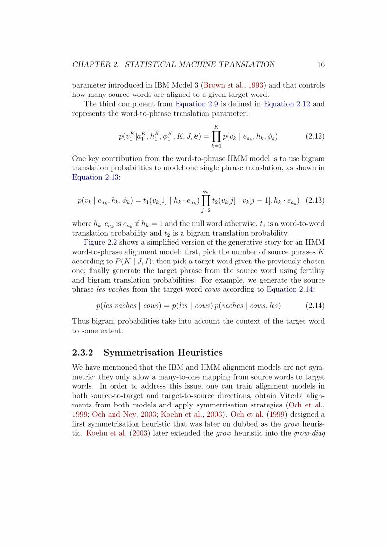
where hk ·eak is eak if hk = 1 and the null word otherwise, t1 is a word-to-wordtranslation probability and t2 is a bigram translation probability.
Figure 2.2 shows a simplified version of the generative story for an HMMword-to-phrase alignment model: first, pick the number of source phrases Kaccording to P (K | J, I); then pick a target word given the previously chosenone; finally generate the target phrase from the source word using fertilityand bigram translation probabilities. For example, we generate the sourcephrase les vaches from the target word cows according to Equation 2.14:
p(les vaches | cows) = p(les | cows) p(vaches | cows , les) (2.14)
Thus bigram probabilities take into account the context of the target wordto some extent.
2.3.2 Symmetrisation Heuristics
We have mentioned that the IBM and HMM alignment models are not sym-metric: they only allow a many-to-one mapping from source words to targetwords. In order to address this issue, one can train alignment models inboth source-to-target and target-to-source directions, obtain Viterbi align-ments from both models and apply symmetrisation strategies (Och et al.,1999; Och and Ney, 2003; Koehn et al., 2003). Och et al. (1999) designed afirst symmetrisation heuristic that was later on dubbed as the grow heuris-tic. Koehn et al. (2003) later extended the grow heuristic into the grow-diag

CHAPTER 2. STATISTICAL MACHINE TRANSLATION 17
..The. wolf. loves. fat. cows.
p(K = 5 | I = 5, J = 6)
.
Le
.
loup
.
aime
.
les vaches
.
grasses
.
φ1 = 1
.
φ2 = 1
.
φ3 = 1
.
φ5 = 1
.
φ4 = 2
.
p(2 | 1)
.
p(3 | 2)
.
p(5 | 3)
.p(4 | 5)
Figure 2.2: Simplified generative story for an HMM word-to-phrase alignmentmodel. Adapted from (Deng and Byrne, 2008). The adjective noun sequencefat cows is reordered into the noun adjective sequence vaches grasses. Theword cows has fertility 2 as it is translated into the target phrase les vaches.
and grow-diag-final heuristics and examined the impact on translation per-formance for each heuristic.
Alignments from source to target (i.e. in which the alignment is a func-tion from source positions to target positions) and target to source are de-noted af2e and ae2f respectively. Let us consider a sentence pair (f , e), andsource-to-target and target-to-source Viterbi alignments af2e and ae2f . Theintersection and union heuristics are defined as follows:
• intersection: a = ae2f ∩ af2e
• union: a = ae2f ∪ af2e
The intersection heuristics typically produces high precision alignments whilethe union heuristics typically produces high recall alignments (Och and Ney,2003). We now present the grow heuristic and its variants, which are basedon the initial intersection and union heuristics. The grow heuristic algorithmis presented in Figure 2.3. The input is a sentence pair (fJ
1 , eI1), a source-to-
target alignment af2e and a target-to-source alignment ae2f . The resultingalignment a is initialised with the intersection (line 2). Then alignment links

CHAPTER 2. STATISTICAL MACHINE TRANSLATION 18
1: function Grow(fJ1 , e
J1 ,af2e,ae2f )
2: a← af2e ∩ ae2f
3: while true do4: added ← false5: for i ∈ [1, I] do6: for j ∈ [1, J ] do7: if (j, i) ∈ a then8: for (k, l) ∈ Neighbours((j, i)) ∩(af2e ∪ ae2f ) do9: if k not aligned in a or l not aligned in a then
10: a← a ∪ (k, l)11: added ← true12: end if13: end for14: end if15: end for16: end for17: if not added then18: break19: end if20: end while21: return a22: end function
Figure 2.3: Algorithm for the grow symmetrisation heuristic (Koehn, 2010).The alignment is initialised from the intersection and alignment links thatare neighbours to existing alignment links are iteratively added if the sourceor the target is not already aligned.

CHAPTER 2. STATISTICAL MACHINE TRANSLATION 19
that are in the union and that are neighbours of already existing alignmentlinks (line 8) are considered. If the source or the target word is not alreadyaligned (line 9), then the link is added to the resulting alignment (line 10).This is repeated until no more links are added.
In the grow heuristic, neighbours are defined as horizontal or verticalneighbours. If diagonal neighbours are also considered, then the heuristicbecomes grow-diag. The grow heuristic also has an optional step called final.Alignment links in the union where the source or the target is not alreadyaligned can also be added to the resulting alignment. If only links in theunion where the source and the target are not already aligned are consideredfor the final procedure, then the optional step is called final-and.
Symmetrisation heuristics have been shown to be beneficial for alignmentsboth in terms of alignment quality as measured by comparing automaticalignments to human alignments and in translation quality when alignmentsare used as an intermediate step in the translation pipeline.
2.4 Log-Linear Model of Machine TranslationAs we have seen in Section 2.2, SMT was historically framed as a source-channel model. As an alternative, Berger et al. (1996) introduce maximumentropy models for natural language processing. In maximum entropy mod-elling, we wish to estimate a conditional probability p(y | x). Given atraining sample, various feature functions deemed to be relevant are picked.We then constrain p such that the expected value of each feature function fwith respect to the empirical distribution is equal to the expected value off with respect to the model p. Finally, p is chosen among all models thatsatisfy the constraints defined by the features and such that its entropy ismaximum. Berger et al. (1996) show how a maximum entropy model can beparameterised as an exponential, or log-linear model. They apply this modelto three machine translation related tasks. First, they use a maximum en-tropy model to predict the translation of a word using the context for thatword. Then, they use a maximum entropy model to predict the target lan-guage word order. Finally, they apply maximum entropy modelling in orderto predict the source sentence segmentation.

CHAPTER 2. STATISTICAL MACHINE TRANSLATION 20
Och et al. (1999) notice that using an erroneous version of the source-channel model, that is using the following equation:
e = argmaxe
p(e | f) p(e) (2.15)
gives comparable performance with respect to using the correct formulationof the source-channel model given in Equation 2.1. Then Och and Ney (2002)propose the following log-linear model extension:
e = argmaxe
p(e | f)
= argmaxe
exp(∑M
m=1 λmhm(e,f))∑e′ exp(
∑Mm=1 λmhm(e′,f))
= argmaxe
exp(M∑
m=1
λmhm(e,f)) (2.16)
where hm are called feature functions and λm are called feature weights. Thelog-linear model is an extension to the source-channel model because it canbe reduced to the original source-channel model with the following settings:
• M = 2
• h1(e,f) = log(p(f |e))
• h2(e,f) = log(p(e))
• λ1 = λ2 = 1
Log-linear models were originally trained with the maximum likelihood cri-terion, which precisely makes them equivalent to maximum entropy mod-els (Berger et al., 1996). More effective training techniques such as mini-mum error rate training (Och, 2003) were introduced subsequently (see Sec-tion 2.8.2). An advantage of minimum error rate training is that the criterionfor optimisation and the evaluation metric are consistent. Because minimumerror rate training does not require computing a normalisation constant, inpractice, SMT models effectively become linear models, with the objectivefunction presented in Equation 2.17:
e = argmaxe
M∑m=1
λmhm(e,f) (2.17)

CHAPTER 2. STATISTICAL MACHINE TRANSLATION 21
2.5 Phrase-Based TranslationSo far, we have presented two modelling approaches to machine translation:the original source-channel model and the current log-linear model. We alsohave presented word alignment models, which were introduced within thesource-channel model framework and which are instances of word-based mod-els.
In the phrase-based translation paradigm, the minimal unit of translationconsists of phrases. Phrases are sequences of consecutive words, that neednot be syntactically or semantically motivated, but nevertheless are used astranslation units. Benefits of phrase-based models include:
• effectively disambiguating the translation of a word in a certain localcontext;
• effective local reordering within a phrase such as the adjective-nouninversion from French to English;
• effective translation of multi-word expressions, such as idioms.
Phrase-based models currently achieve state-of-the-art performance for cer-tain language pairs that do not involve much reordering such as French-English. They can be defined in the source-channel model framework (seeSection 2.2) or the log-linear model framework (see Section 2.4). Becausethe source-channel model is no longer widely used anymore and because itis a special case of a log-linear model, we will focus our presentation on thelog-linear model.
There are different variations on the phrase-based translation paradigm.We will focus on two popular approaches, namely the alignment templatemodel (Och et al., 1999; Och and Ney, 2004) and the phrase-based model (Koehnet al., 2003; Koehn, 2010).
2.5.1 Alignment Template Model
The alignment template model uses the log-linear model presented in Equa-tion 2.16 as a starting point and repeated in Equation 2.18:
e = argmaxeJ1
exp(M∑
m=1
λmhm(fJ1 , e
I1)) (2.18)

CHAPTER 2. STATISTICAL MACHINE TRANSLATION 22
In order to reduce the number of parameters, two latent variables πK1 and
zK1 are introduced. zK1 is a sequence of alignment templates while πK1 is a
permutation of size K. An alignment template is a triple (F , E, A) where Fis a sequence of source word classes, E is a sequence of target word classesand A is an alignment between F and E. πK
1 together with zK1 define a sourcesegmentation of fJ
1 into source phrases fK1 , a target segmentation of eI1 into
target phrases eK1 and a bijective mapping between source phrases and targetphrases where fπk
is mapped to ek for k ∈ [1, K]. The alignment templateszK1 are constrained in such a way that the alignment template classes matchthe word classes. The alignment template translation model is summarisedin Figure 2.4.
Using the max approximation and making the feature functions depend onthe hidden variables, the translation model can be rewritten in Equation 2.19:
e = argmaxeJ1 ,z
K1 ,πK
1
exp(M∑
m=1
λmhm(fJ1 , e
I1, π
K1 , zK1 )) (2.19)
2.5.2 Phrase-Based Model
The phrase-based model is similar to the alignment template model but doesnot make use of source and target word classes. Again, we use the latentvariables πK
1 and zK1 . This time, zk is defined as a triple (f , e, A) where fis a sequence of source words, e is a sequence of target words and A is analignment between the words in f and e. The reason for using the alignmentinformation between phrase pairs is to be able to compute the lexical feature(see Section 2.6.5). Because the lexical feature can be computed by othermeans than this alignment information (see again Section 2.6.5), it is alsopossible to simply define zk as a phrase pair.
We have presented two variants of the phrase-based model. We will nowdescribe how to obtain the phrase pairs used for the latent variable z.
2.5.3 Phrase Pair Extraction
A preliminary step to phrase pair extraction is to obtain word aligned paralleltext. One possibility is to train source-to-target and target-to-source wordalignment models, obtain Viterbi alignments in both directions, and applysymmetrisation heuristics, as described in Section 2.3.2. Then phrase pairsare extracted from each word aligned sentence pair.

CHAPTER 2. STATISTICAL MACHINE TRANSLATION 23
..f1. f2. f3. f4. f5. f6. f7.
f1
.
f2
.
f3
.
f4
.
f5
.
f6
.
f7
.
f1
.
f2
.
f3
.
f4
.
e1
.
e2
.
e3
.
e4
.
e2
.
e1
.
e3
.
e4
.
e5
.
e6
.
e1
.
e2
.
e3
.
e4
.
e5
.
e6
.
z1
.
z2
.
z3
.
z4
Figure 2.4: Alignment template translation process. Adapted from (Och andNey, 2004). The source word sequence f 7
1 is first transformed into a sourceclass sequence f
7
1. The source classes are then segmented into source phrasesf 41 . The source phrases are then reordered and aligned to target phrases e41.
For example, the source phrase f1 is aligned to the target phrase e2 throughz1. This means that the permutation π4
1 has value π2 = 1. This also meansthat z1 define a word alignment between the source words f1 and f2 and thetarget word e3. Finally, the target phrases e41, which encode the target classsequence e61 generate the target word sequence e61.

CHAPTER 2. STATISTICAL MACHINE TRANSLATION 24
..El. mundo. es. grande.
The
.
world
.
is
.
big
..
Figure 2.5: Rule extraction for a sentence pair. For example, the phrase(El mundo, The world) is extracted. The phrase pair (es grande, big) is notextracted because it is not consistent with the alignment.
Let us consider a sentence pair (f , e) and an alignment a. We extract allphrase pairs that are consistent with the alignment. This means that we ex-tract all phrase pairs (f j2
j1, ei2i1) that satisfy Equation 2.20 and Equation 2.21:
∀(j, i) ∈ a, (j ∈ [j1, j2]⇔ i ∈ [i1, i2]) (2.20)[j1, j2]× [i1, i2] ∩ a 6= ∅ (2.21)
Equation 2.20 requires that no alignment link be between a word inside thephrase pair and a word outside the phrase pair. Equation 2.21 requires thatthere be at least one alignment link between a source word in the sourcephrase and a target word in the target phrase. For example, in Figure 2.5,the phrase pair 〈El mundo, The world〉 is extracted while the phrase pair 〈esgrande, big〉 is not because the word es (is) is aligned outside the phrase pair.Note that the consistency constraint sometimes refers to only Equation 2.20rather than both Equation 2.20 and Equation 2.21.
2.5.4 Phrase-Based Decoding
We have introduced two types of phrase-based models and described a tech-nique to extract phrase-pairs, which are an essential component of thesemodels. We will now describe the decoding process, which is an effectivemeans to obtain the optimal translation of a source sentence.
We first describe a naive strategy for decoding, in order to motivate theneed for a more efficient decoder. A naive decoder may follow the followingsteps, given a source sentence f of length J to be translated:

CHAPTER 2. STATISTICAL MACHINE TRANSLATION 25
• Consider all possible segmentations of f into source phrases. There are2J−1 such segmentations.
• For each segmentation, consider all possible permutations of the sourcephrases. For a segmentation of size K, there are K! such permutations.
• For each permutation of the source phrases, consider all translations ofeach source phrase, and concatenate the target phrases according to thepermutation. The source phrases translations are given by the phrasepairs extracted from the training data (see Section 2.5.3). If there are10 translations per source phrase, we obtain 10K possible translation(for the segmentation and permutation considered).
• Rank the translations by their score and pick the highest scoring trans-lation.
We can see that the search space is too large for this naive approach tobe feasible. We now present a practical solution to the decoding processin phrase-based translation. We will first introduce the translation process.Then, we will describe how translation hypotheses are built incrementally.We will then motivate the need for pruning and how pruning is carried out.Finally, we will describe how future cost estimation may reduce search errors.
Translation Process Given a source sentence, the translation process isto iteratively pick a source phrase that has not been translated yet, translatethat source phrase into a target phrase and append the target phrase tothe translation, and repeat this process until the source sentence has beenentirely covered by source phrases. While the process is not complete, theconcatenation of target phrases is called a partial hypothesis.
Hypothesis Expansion The decoding process starts from an initial emptypartial hypothesis. This empty partial hypothesis is extended by pickingsource phrases, appending their translations to the empty hypothesis. At thisstage, we have obtained several partial hypotheses. The partial hypothesesare repeatedly extended until all source words have been covered. Partialhypotheses are represented by states that contain the information necessaryto compute the cost of an extension. If we use an n-gram language modelas a feature, the state will encode the cost of the partial hypothesis and thelast n− 1 words of the partial hypothesis.
CHAPTER 2. STATISTICAL MACHINE TRANSLATION 26
Hypothesis Recombination When two partial hypotheses share the samen− 1 words, only the partial hypothesis with the lower cost can lead to thebest final hypothesis. Therefore, the partial hypothesis with higher cost canbe discarded, or alternatively, it is possible to make these two partial hy-potheses share the same state for rescoring purposes.
Stack Based Decoding and Pruning The decoding search space is verylarge as seen above. Approximations therefore need to be made for an ef-fective search. The partial hypotheses are grouped in stacks by the numberof source words covered. This allows pruning. Each time a hypothesis ex-pansion produces a hypothesis that belongs to a certain stack, that stack ispruned. There are two commonly used types of pruning: histogram prun-ing and threshold pruning (Koehn, 2010). Histogram pruning enforces amaximum number of partial hypotheses in each stack. Threshold pruningexamines the cost of the best partial hypothesis in a stack and discards allpartial hypotheses in that stack whose cost is greater than the best costplus a threshold. Histogram pruning provides a simple guarantee in termsof computational complexity. On the other hand, because it relies on cost,threshold pruning ensures a consistent quality for partial hypotheses thatsurvive the pruning threshold.
Future Cost Partial hypotheses that cover the same number of sourcewords are grouped together for pruning purposes. However, their cost maynot be directly comparable, for example partial hypotheses that correspondto the translation of frequent words in the source might have a smaller costthan partial hypotheses that correspond to the translation of rare words inthe source. To address this issue, a future cost that represents how difficultit is to translate the rest of the sentence is added to the model cost of eachpartial hypothesis.
2.6 Hierarchical Phrase-Based TranslationIn the previous section, we have described the phrase-based translationparadigm. In this section, we present the hierarchical phrase-based trans-lation model. This model relies on the synchronous context free grammarformalism. Reordering between source and target languages is modelled bythe grammar rather than by an ad hoc reordering model, although using both

CHAPTER 2. STATISTICAL MACHINE TRANSLATION 27
the grammar and a reordering model may be beneficial (Huck et al., 2013). Aclosely related formalism, inversion transduction grammars, was previouslyintroduced (Wu, 1995, 1997). However, because hierarchical phrase-basedgrammar only contain lexicalised rules, translation decoding is more practi-cal. An alternative to hierarchical phrase-based translation that also modelsdiscontinuous phrases but does not use the same grammar formalism has alsobeen introduced recently (Galley and Manning, 2010).
2.6.1 Introduction and Motivation
Phrase-based models generally impose a limit on the size of the phrase pairsextracted while, in decoding, phrases are typically reordered within a cer-tain limit. These restrictions may be problematic for language pairs such asGerman-English or Chinese-English that allow arbitrary reordering in someinstances. Hierarchical phrase-based translation was introduced in order toovercome the reordering limitations from phrase-based models (Chiang, 2005,2007). For example, the Chinese sentence with English gloss in Figure 2.6requires “nested” reordering (Chiang, 2007):• The phrase with North Korea have diplomatic relations must be re-
ordered into the phrase have diplomatic relations with North Korea.
• The phrase few countries one of must be reordered into the phrase oneof (the) few countries.
• After the two previous segments are reordered, have diplomatic rela-tions with North Korea that one of the few countries must be reorderedinto one of the few countries that have diplomatic relations with NorthKorea.
Phrase-based systems can model this type of movement but they require verylong phrase pairs, which is impractical to rely upon because of data sparsity.On the other hand, hierarchical phrase-based grammars do model this typeof movement using shorter phrase pairs but with more complex rules.
2.6.2 Hierarchical Grammar
2.6.2.1 Hierarchical Grammar Definition
A hierarchical phrase-based grammar, or hierarchical grammar, or Hierogrammar, which is a particular instance of a synchronous context free gram-

CHAPTER 2. STATISTICAL MACHINE TRANSLATION 28
..澳洲. 是. 与. 北韩. 有. 邦交. 的. 少数. 国家. 之一.
Australia
.
is
.
with
.
NorthKorea
.
have
.
diplomaticrelations
.
that
.
few
.
countries
.
oneof
.
Australia
.
is
.
oneof
.
thefew
.
countries
.
that
.
have
.
diplomaticrelations
.
with
.
NorthKorea
Figure 2.6: Example of Chinese sentence that needs nested reordering inorder to be translated into English. Adapted from (Chiang, 2007).
mar (Lewis II and Stearns, 1968; Aho and Ullman, 1969), is a set of rewriterules of the following type:
X → 〈γ, α,∼〉
where X is a nonterminal, γ and α are sequences of terminals and nontermi-nals and ∼ is an alignment between nonterminals. Terminals that appear in γare words in the source language while terminals that appear in α are wordsin the target language. Nonterminals are chosen from a finite set disjointfrom the set of terminals. The alignment between nonterminals indicateswhich nonterminals in the source and target languages correspond to eachother. The alignment ∼ can be written with a set of matching indices.
2.6.2.2 Types of Rules
A rule may or may not contain any nonterminals. A rule without nonter-minals (on the right hand side) is called a phrase-based rule. A rule withnonterminals is called a hierarchical rule. A hierarchical grammar also usu-
CHAPTER 2. STATISTICAL MACHINE TRANSLATION 29
R1 : S → 〈X,X〉R2 : S → 〈SX, SX〉R3 : X → 〈X1 的 X2, the X2 that X1〉R4 : X → 〈X 之一, one of X〉R5 : X → 〈与 X1 有 X2, have X2 with X1〉R6 : X → 〈澳洲, Australia〉R7 : X → 〈是, is〉R8 : X → 〈北韩, North Korea〉R9 : X → 〈邦交, diplomatic relations〉R10 : X → 〈少数 国家, few countries〉
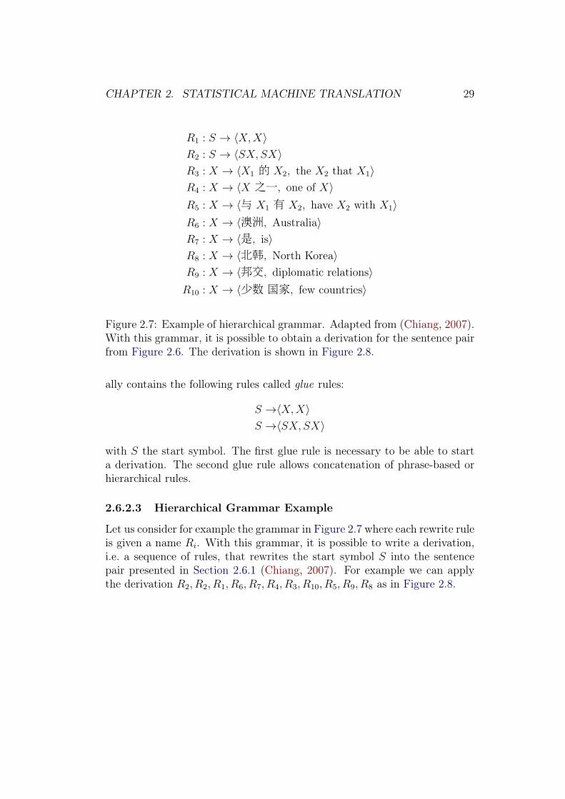
Figure 2.7: Example of hierarchical grammar. Adapted from (Chiang, 2007).With this grammar, it is possible to obtain a derivation for the sentence pairfrom Figure 2.6. The derivation is shown in Figure 2.8.
ally contains the following rules called glue rules:
S →〈X,X〉S →〈SX, SX〉
with S the start symbol. The first glue rule is necessary to be able to starta derivation. The second glue rule allows concatenation of phrase-based orhierarchical rules.
2.6.2.3 Hierarchical Grammar Example
Let us consider for example the grammar in Figure 2.7 where each rewrite ruleis given a name Ri. With this grammar, it is possible to write a derivation,i.e. a sequence of rules, that rewrites the start symbol S into the sentencepair presented in Section 2.6.1 (Chiang, 2007). For example we can applythe derivation R2, R2, R1, R6, R7, R4, R3, R10, R5, R9, R8 as in Figure 2.8.

CHAPTER 2. STATISTICAL MACHINE TRANSLATION 30
S → 〈SX, SX〉→ 〈SX1X2, SX1X2〉→ 〈X1X2X3, X1X2X3〉→ 〈澳洲 X2X3,Australia X2X3〉→ 〈澳洲 是 X3,Australia is X3〉→ 〈澳洲 是 X 之一,Australia is one of X〉→ 〈澳洲 是 X1 的 X2 zhiyi,Australia is one of the X2 that X1〉→ 〈澳洲 是 X1 的 少数 国家 之一,Australia is one of the few countries that X1〉→ 〈澳洲 是 与 X1 有 X2 的 少数 国家 之一,
Australia is one of the few countries that have X2 with X1〉→ 〈澳洲 是 与 X1 有 邦交 的 少数 国家 之一,
Australia is one of the few countries that have diplomatic relations with X1〉→ 〈澳洲 是 与 北韩 有 邦交 的 少数 国家 之一,
Australia is one of the few countries that have diplomatic relations with North Korea〉
Figure 2.8: Example of hierarchical grammar derivation. Adapted from (Chi-ang, 2007). A derivation is simply a sequence of rules that rewrite the startsymbol S into a sentence pair. This particular derivation produces the sen-tence pair from Figure 2.6.

CHAPTER 2. STATISTICAL MACHINE TRANSLATION 31
2.6.2.4 Constraints on Hierarchical Grammars
The definition given for a hierarchical grammar is very general. In prac-tice, systems impose constraints on the types of rule the grammar con-tains for efficiency reasons. We first introduce the concept of rule pat-tern (Iglesias et al., 2009a) in order to describe these constraints in termsof patterns. A rule pattern is simply a pair of regular expressions thatmatch the source and target sides of a hierarchical rule. For example,the rule X → 〈Buenas tardes X, Good afternoon X〉 has a rule pattern〈Σ+X,Ψ+X〉 where Σ is the source vocabulary and Ψ is the target vocabu-lary. For ease of notation, we use the notation w for either Σ+ or Ψ+. Thusw simply represents a sequence of terminals. In our example, the pattern forthe rule X → 〈Buenas tardes X, Good afternoon X〉 is 〈wX,wX〉. Chiang(2007) defines the following set of pattern-related constraints that must besatisfied by the rules in a hierarchical grammar:
• If a rule X → 〈γ, α〉 has a pattern 〈w,w〉, then |γ| ≤ 10 and |α| ≤ 10.
• A rule X → 〈γ, α〉 must satisfy |γ| ≤ 5.
• Rules have at most 2 nonterminals.
• The source side of a rule cannot have adjacent nonterminals. Setiawanand Resnik (2010) relax this constraint in order to model Chinese-English reordering phenomena that may be not always captured intraining because of data sparsity. Note that the target side can stillhave adjacent nonterminals.
More fine-grained constraints can be defined on rule patterns, which are ob-tained from rules by replacing terminal sequences by the placeholder w. Forexample, we use the configuration described in Table 2.1 for all translationexperiments in this thesis, unless specified otherwise. This grammar wasobtained following a greedy strategy of adding in turn the most beneficialpatterns for Arabic-English translation.
Another restriction on hierarchical grammars is the extent of reorderingallowed. de Gispert et al. (2010a) investigate the use of shallow-N grammarsthat precisely control the depth of reordering in translation. We describe hereshallow-1 grammars (Iglesias et al., 2009a; de Gispert et al., 2010a) as theywill be used for translation experiments in this thesis. Shallow-1 grammarsallow only one level of reordering, they do not allow nested reordering as in

CHAPTER 2. STATISTICAL MACHINE TRANSLATION 32
〈source , target〉 include 〈source , target〉 include〈w X , w X〉 no 〈X w , w X〉 yes〈w X , X w〉 yes 〈X w , w X w〉 yes〈w X , w X w〉 yes 〈X w , X w〉 no
〈w X w , w X〉 yes 〈w X w , X w〉 yes〈w X w , w X w〉 yes
〈X1 w X2 , w X1 w X2〉 no 〈X2 w X1 , w X1 w X2〉 yes〈X1 w X2 , w X1 w X2 w〉 no 〈X2 w X1 , w X1 w X2 w〉 yes〈X1 w X2 , w X1 X2〉 no 〈X2 w X1 , w X1 X2〉 yes〈X1 w X2 , w X1 X2 w〉 no 〈X2 w X1 , w X1 X2 w〉 yes〈X1 w X2 , X1 w X2〉 no 〈X2 w X1 , X1 w X2〉 yes〈X1 w X2 , X1 w X2 w〉 no 〈X2 w X1 , X1 w X2 w〉 yes〈X1 w X2 , X1 X2 w〉 no 〈X2 w X1 , X1 X2 w〉 yes
〈w X1 w X2 , w X1 w X2〉 no 〈w X2 w X1 , w X1 w X2〉 yes〈w X1 w X2 , w X1 w X2 w〉 yes 〈w X2 w X1 , w X1 w X2 w〉 yes〈w X1 w X2 , w X1 X2〉 yes 〈w X2 w X1 , w X1 X2〉 yes〈w X1 w X2 , w X1 X2 w〉 yes 〈w X2 w X1 , w X1 X2 w〉 yes〈w X1 w X2 , X1 w X2〉 yes 〈w X2 w X1 , X1 w X2〉 yes〈w X1 w X2 , X1 w X2 w〉 yes 〈w X2 w X1 , X1 w X2 w〉 yes〈w X1 w X2 , X1 X2 w〉 yes 〈w X2 w X1 , X1 X2 w〉 yes〈X1 w X2 w , w X1 w X2〉 yes 〈X2 w X1 w , w X1 w X2〉 yes〈X1 w X2 w , w X1 w X2 w〉 yes 〈X2 w X1 w , w X1 w X2 w〉 yes〈X1 w X2 w , w X1 X2〉 yes 〈X2 w X1 w , w X1 X2〉 yes〈X1 w X2 w , w X1 X2 w〉 yes 〈X2 w X1 w , w X1 X2 w〉 yes〈X1 w X2 w , X1 w X2〉 yes 〈X2 w X1 w , X1 w X2〉 yes〈X1 w X2 w , X1 w X2 w〉 no 〈X2 w X1 w , X1 w X2 w〉 yes〈X1 w X2 w , X1 X2 w〉 yes 〈X2 w X1 w , X1 X2 w〉 yes
〈w X1 w X2 w , w X1 w X2〉 no 〈w X2 w X1 w , w X1 w X2〉 yes〈w X1 w X2 w , w X1 w X2 w〉 no 〈w X2 w X1 w , w X1 w X2 w〉 yes〈w X1 w X2 w , w X1 X2〉 no 〈w X2 w X1 w , w X1 X2〉 yes〈w X1 w X2 w , w X1 X2 w〉 no 〈w X2 w X1 w , w X1 X2 w〉 yes〈w X1 w X2 w , X1 w X2〉 no 〈w X2 w X1 w , X1 w X2〉 yes〈w X1 w X2 w , X1 w X2 w〉 no 〈w X2 w X1 w , X1 w X2 w〉 yes〈w X1 w X2 w , X1 X2 w〉 no 〈w X2 w X1 w , X1 X2 w〉 yes
Table 2.1: Rule patterns included in a baseline hierarchical grammar. Apattern is obtained from a rule by replacing terminal sequences by the place-holder w. The decision whether to include each pattern was based on prelim-inary experiments in Arabic-English. Most beneficial patterns were addedincrementally. Unless specified otherwise, this configuration is used in allsubsequent translation experiments.

CHAPTER 2. STATISTICAL MACHINE TRANSLATION 33
the example presented in Section 2.6.1. A shallow-1 grammar is defined asfollows:
S → 〈X,X〉S → 〈SX, SX〉X → 〈γs, αs〉(γs, αs ∈ (T ∪ {V })+)X → 〈V, V 〉V → 〈s, t〉(s ∈ T+, t ∈ T ∗)
where S is the start symbol, T is the set of terminals and V is the set ofnonterminals. There are two nonterminals apart from the start symbol: Xand V . The rule type X → 〈γs, αs〉 corresponds to all hierarchical rules. Itis possible to apply this type of rule only once in any derivation. Indeed,the right hand side contains only one type of nonterminal, V , which canbe rewritten only with a phrasal rule corresponding to the line V → 〈s, t〉.Note that for rules of the type V → 〈s, t〉, t can be the empty word, thusthese rules, called deletion rules, allow deletion on the target side. Shallow-1grammar are used for language pairs that do not present much reordering.Shallow-1 grammars were previously shown to work as well as full hierarchicalgrammars for the Arabic-English language pair (Iglesias et al., 2009a) andfor the Spanish-English language pair (Iglesias et al., 2009c). In addition,shallow-1 grammars reduce the search space of the decoder greatly, resultingin a much faster decoding time, a reduced memory use and potentially fewersearch errors under the translation grammar.
2.6.3 Log-linear Model for Hierarchical Phrase-BasedTranslation
We now define in more detail the log-linear model for hierarchical translation,which usually makes a maximum (max) approximation, i.e. replaces a sumby the maximum term in the sum and assumes that the other terms arenegligible. We follow the original description (Chiang, 2007). For a sentencepair (f , e), let us define D the set of possible derivations D of this sentencepair under a hierarchical grammar. We will use the following notation for aderivation D:
• the foreign yield f . We define f(D) = f

CHAPTER 2. STATISTICAL MACHINE TRANSLATION 34
• the English yield e. We define e(D) = e
We can now derive the log-linear model for hierarchical translation:
e = argmaxe
p(e | f)
= argmaxe
∑D∈D
p(D, e | f) (marginalisation)
= argmaxe
argmaxD∈D
p(D, e | f) (max approximation)
= e(argmaxe,D∈D
p(D, e|f))
= e(argmaxD|f(D)=f
p(D)) (2.22)
Thanks to the max approximation, the distribution over derivations in-stead of the distribution over English sentences is modelled log-linearly andwe obtain finally the following decoding equation:
e = e(argmaxD|f(D)=f
exp(M∑
m=1
λmhm(D))) (2.23)
One of the features, the language model, plays a particular role. The languagemodel feature can be written as:
hM(D) = pLM(e(D)) (2.24)
where M is the index of the language model feature, pLM is the languagemodel and e(D) is the English yield of the derivation D. It is not possible tocompute the language model using dynamic programming since the languagemodel needs context in order to be computed, therefore the language modelfeature is typically computed after a parsing step.
Note that Equation 2.23 is an approximation and that there have beenattempts to perform marginalisation over the latent variable D while keep-ing the translation process tractable (Blunsom et al., 2008a; de Gispertet al., 2010a). This can give gains over the max approximation, althoughsubsequent rescoring steps (see Section 2.10) can produce similar perfor-mance (de Gispert et al., 2010a).

CHAPTER 2. STATISTICAL MACHINE TRANSLATION 35
2.6.4 Rule Extraction
We have so far given the definition of a hierarchical grammar and explainedhow it is used with statistical models. It is also necessary to extract anappropriate grammar, defined by its rules. The extraction is performed ona parallel corpus. The parallel corpus is first word-aligned, then rules areextracted from the alignment.
We first extract phrase pairs as described in Section 2.5.3. For eachextracted phrase pair 〈f j2
j1, ei2i1〉, we define the following rule: X → 〈f j2
j1, ei2i1〉.
These rules are called initial rules. We extend the set of initial rules withthe following recursion: given a rule X → 〈γ, α〉 and an initial rule X →〈f j2
j1, ei2i1〉 such that γ = γ1f
j2j1γ2 and α = α1e
i2i1α2, then extract the rule
X → 〈γ1Xγ2, α1Xα2〉. Note that γ1 or γ2, but not both, can be the emptyword, and similarly for α1 and α2.
2.6.5 Features
The following features are commonly used in log-linear models for machinetranslation:
• Source-to-target and target-to-source translation models. As describedabove, the translation process produces a derivation D. A derivationD can be seen as a sequence of n rules X → 〈α1, γ1〉, ..., X → 〈αn, γn〉.Then the source-to-target translation model is simply
∏ni=1 p(γi|αi)
where the p(γi|αi) are typically estimated using relative frequency,based on the appearance of phrasal and hierarchical rules in the parallelcorpus. The target-to-source translation model is symmetric.
• Source-to-target and target-to-source lexical translation model. Typi-cally, the source-to-target lexical translation model lx(fJ
1 , eI1) is com-
puted as following for a foreign sentence fJ1 translated into the English
sentence eI1:
lx(fJ1 , e
I1) =
1
(I + 1)J
J∏j=1
I∑i=0
p1(ei|fj) (2.25)
where p1 is the word-to-word translation probability in IBM Model 1and e0 the null word. The target-to-source lexical translation model issymmetric. One reason to use lexical models in addition to translation

CHAPTER 2. STATISTICAL MACHINE TRANSLATION 36
models is that translation models are relatively sparse compared tolexical models, thus lexical models can smooth the translation models.
• Number of uses of the glue rule in a derivation. This feature trades offmonotonic translation versus reordering.
• Word insertion penalty. This feature controls the length of the output.
• Rule insertion penalty. This feature controls the number of rules usedin a derivation to generate a translation. Using many rules is closerto word-to-word translation while using few rules means that longerphrase pairs are used. This feature is similar to the phrase penalty inphrase-based statistical machine translation (Koehn, 2010).
• Word deletion scale factor. This feature controls the number of timesa deletion rule is applied.
• Rule count feature. This feature indicates whether a rule occurs once,twice or more in the parallel data (Bender et al., 2007). Thus it indi-cates how reliable a rule is.
The feature weights are optimised using minimum error rate training (Och,2003) under the BLEU score (Papineni et al., 2002) (see also Section 2.8.1).
2.7 Language ModellingWe mentioned in Section 2.6.3 that a language model was one of the fea-tures of log-linear models for translation. This feature is critical as it helpsto obtain a fluent translation output. A language model is a probabilitydistribution over word sequences. It can be used to assign a probability toa sequence of words or to predict the word most likely to appear in a cer-tain context. Language models have applications in fields where the goal isto produce fluent output, such as automatic speech recognition or machinetranslation. n-gram language models are typically used because they arerobust, can be easily trained on large amounts of data and model local gram-matical relationships. Since they do not model the language structure norlong distance relationships between words, work has been conducted (Shenet al., 2008) to overcome this issue. We first review n-gram language models,then review different smoothing techniques and we finally describe in more

CHAPTER 2. STATISTICAL MACHINE TRANSLATION 37
detail two smoothing techniques that are used for experiments in this thesis:Kneser-Ney smoothing and Stupid Backoff smoothing.
2.7.1 n-gram language models
For simplicity, let us first consider the case of a bigram language model.Let us consider a vocabulary V and the two special symbols <s> and </s>corresponding respectively to the start-of-sentence symbol and the end-of-sentence symbol. We define W = V ∪ {<s>, </s>}. Let us now define theMarkov chain (Xi)i∈N with values in W and transition probability p. p hasthe following properties:
• p(X0 = <s>) = 1: we always start a sentence with a start-of-sentencesymbol.
• p(Xn+1 = </s> | Xn = </s>) = 1: once we reach the end of a sentence,we stay in the end-of-sentence state. This is because we do not considerinfinite word sequences.
• p(Xn+1 = <s> | Xn = <s>) = 0: we cannot stay in the start-of-sentencestate and have to transition to either a word or the end-of-sentencestate.
A bigram model is defined by the conditional independence assumptions ofthe Markov chain (Xi) and the translation probability p. A bigram modelwill therefore assign the probability p(w) to a sequence of words w = w1...wn
in Equation 2.26:
p(w) =n+1∏i=1
p(wi | wi−1) (2.26)
with the convention w0 = <s> and wn+1 = </s>.An n-gram language model can be defined similarly: this time the random
variables Xi take values in W n−1 instead of W . An n-gram model will assignthe probability p(w) to a sequence of words w = w1...wn in Equation 2.27:
p(w) =n+1∏i=1
p(wi | wi−1i−n+1) (2.27)
with the same convention that w0 = <s> and wn+1 = </s>. Parame-ters can be trained using maximum likelihood estimation, so the parameter

CHAPTER 2. STATISTICAL MACHINE TRANSLATION 38
p(wi|wi−1i−n+1) is computed in Equation 2.28.
p(wi|wi−1i−n+1) =
c(wii−n+1)
c(wi−1i−n+1)
(2.28)
where c(.) counts the number of occurrences of a particular word sequence inthe training data. Maximum likelihood estimation assigns zero probabilityto unseen events, therefore different smoothing strategies have been exploredto address this problem.
2.7.2 Back-off and Interpolated Models
Smoothing strategies for language modelling make use of lower order dis-tributions either by backoff or interpolation. The general form of a backoffmodel (Chen and Goodman, 1998) is presented in Equation 2.29:
pbackoff(wi | wi−1i−n+1) =
{α(wi | wi−1
i−n+1) if c(wii−n+1) > 0
γ(wi−1i−n+1)pbackoff(wi | wi−1
i−n+2) if c(wii−n+1) = 0
(2.29)where c is an occurrence count in the monolingual training corpus for ann-gram. The conditions c(wi
i−n+1) > 0 and c(wii−n+1) = 0 can be replaced by
c(wii−n+1) ≥ cutoff and c(wi
i−n+1) < cutoff respectively when n-grams withan occurrence less than the cutoff threshold are ignored in the training data.
The general form of an interpolated model (Chen and Goodman, 1998)is presented in Equation 2.30:
pinterpolate(wi | wi−1i−n+1) = λwi−1
i−n+1pML(wi | wi−1
i−n+1)+
(1− λwi−1i−n+1
)pinterpolate(wi | wi−1i−n+2)
(2.30)
where:
• pML is the maximum likelihood estimate.
• λwi−1i−n+1
is the interpolation parameter.
The difference between backoff and interpolated model is that interpolatedmodels make use of lower order distributions even when the n-gram countsare greater than zero. However, an interpolated model can be written in theform of a backoff model. Let us define α(wi | wi−1
i−n+1) in Equation 2.31:
α(wi | wi−1i−n+1) = pinterpolate(wi | wi−1
i−n+1) (2.31)

CHAPTER 2. STATISTICAL MACHINE TRANSLATION 39
and γ(wi−1i−n+1) in Equation 2.32:
γ(wi−1i−n+1) = 1− λwi−1
i−n+1(2.32)
We can see that by plugging in the definitions of α(wi | wi−1i−n+1) and γ(wi−1
i−n+1)in Equation 2.29, it is possible to write an interpolated model as a backoffmodel. This observation is trivial but it is useful in practice in order to makeuse of the ARPA file format3 which only supports back-off models.
2.7.3 Modified Kneser-Ney Smoothing
In this section, we present interpolated modified Kneser-Ney smoothing (Chenand Goodman, 1998), which is the most popular smoothing strategy used formachine translation. The motivation for Kneser-Ney smoothing (Kneser andNey, 1995) as given by Chen and Goodman (1998) is that the use of lower or-der distributions for smoothing needs to take into account information fromthe higher order distribution. For example, let us consider a bigram model.We want to assign a probability to the word Francisco given its previousword, say hello. If we have not seen the bigram hello Francisco in the train-ing corpus, we need to back-off to the unigram Francisco. We assume thatthe unigram Francisco is very frequent in our corpus but that it is only seenin the context of the bigram San Francisco. If we simply use the maximumlikelihood estimate of the unigram Francisco, we will obtain a relatively highprobability for the bigram hello Francisco. This should not be the case be-cause the corpus provides evidence that Francisco is very unlikely to followany other word than San.
The modified Kneser-Ney smoothed probability is defined in Equation 2.33.
pKN(wi | wi−1i−n+1) =
c(wii−n+1)−D(c(wi
i−n+1))
c(wi−1i−n+1)
+ γ(wi−1i−n+1)pKN(wi|wi−1
i−n+2)
(2.33)where D and γ are defined in Equation 2.34 and Equation 2.35.
D(c) =
0 if c = 0
D1 if c = 1
D2 if c = 2
D3 if c ≥ 3
(2.34)
3 http://www.speech.sri.com/projects/srilm/manpages/ngram-format.5.html

CHAPTER 2. STATISTICAL MACHINE TRANSLATION 40
γ(wi−1i−n+1) =
D1N1(wi−1i−n+1•) +D2N2(w
i−1i−n+1•) +D3+N3+(w
i−1i−n+1•)
c(wi−1i−n+1)
(2.35)
N1, N2 and N3+ are defined in Equation 2.36.
N1(wi−1i−n+1•) = |{wi : c(wi−n+1wi) = 1}|
N2(wi−1i−n+1•) = |{wi : c(wi−n+1wi) = 2}|
N3+(wi−1i−n+1•) = |{wi : c(wi−n+1wi) ≥ 3}|
(2.36)
2.7.4 Stupid Backoff Smoothing
The Stupid Backoff smoothing scheme (Brants et al., 2007) is similar to thegeneral backoff smoothing scheme presented in Equation 2.29 and presentedin Equation 2.37:
sstupid backoff(wi | wi−1i−n+1) =
c(wi
i−n+1)
c(wi−1i−n+1)
if c(wii−n+1) > 0
α sstupid backoff(wi | wi−1i−n+2) if c(wi
i−n+1) = 0
(2.37)We use the notation s to indicate that that the Stupid Backoff Smoothedscore is not a probability. We note the following differences with respect tothe traditional backoff scheme:• The non backed off score uses no discounting and simply uses relative
frequency.
• The backed off score scaling parameter α is independent of the n-gramhistory.
• As a result, the Stupid Backoff does not define a probability distribu-tion.
Stupid Backoff smoothing was designed to fit the MapReduce framework andbuild very large language models (see Section 3.1). This scheme will be usedin subsequent translation rescoring experiments throughout this thesis.
2.8 Optimisation
2.8.1 Evaluation Metrics
Evaluating the quality of machine translation output is a challenge in thatvery often many possible translations are acceptable and of equal quality. Hu-

CHAPTER 2. STATISTICAL MACHINE TRANSLATION 41
man experts seem to be the most qualified for this task, however their serviceis expensive and time consuming. Automatic metrics have been thereforedesigned in order to allow rapid development and comparison of machinetranslation systems. We describe the BLEU metric since this is the mostwidely used metric and because we use it extensively in our experiments. Werefer to publications for alternative metrics such as METEOR (Banerjee andLavie, 2005), NIST (Doddington, 2002) or TER (Snover et al., 2006).
The BiLingual Evaluation Understudy (BLEU) score (Papineni et al.,2002) is defined as the geometric mean of n-gram modified precisions withrespect to one or several translation references times a brevity penalty. Moreprecisely, given S input sentences s1, ..., sS, we consider a set of S candidatetranslations c1, ..., cS. For each input sentence si, there is a finite number Ri
of reference translations ri,1, ..., ri,Ri. The reference translation that is closest
in length to the candidate translation ci is denoted rci . The BLEU metric isdefined as following:
BLEU(c1, ..., cS, r1,1, ...r1,R1 , ..., rS,1, ..., rS,RS) = BP
N∏n=1
p1Nn (2.38)
BP is the brevity penalty and is defined as:
BP = exp(min(0, 1−∑S
i=1 |rci|∑Si=1 |ci|
)) (2.39)
pn is the modified n-gram precision and is defined as∑Si=1
∑g∈ci countclip(g, ci, ri,1, ..., ri,Ri
)∑Si=1
∑g∈ci count(g, ci)
(2.40)
where g is an n-gram, count(g, ci) is the number of times g occurs in ci and
countclip(g, ci, ri,1, .., ri,Ri) = min(count(g, ci),max(count(g, ri,1), .., count(g, ri,Ri
)))(2.41)
The maximum n-gram order is usually N = 4. The BLEU metric can becomputed efficiently, is language independent and correlates well with humanjudgements, especially for statistical translation systems.

CHAPTER 2. STATISTICAL MACHINE TRANSLATION 42
2.8.2 Minimum Error Rate Training
Minimum error rate training (Och, 2003) is a method to optimise the featureweights in a log-linear model for translation with respect to a particularevaluation metric. We present this method assuming that the evaluationmetric is BLEU. The objective function is defined as follows:
λM1 = argmax
λM1
BLEU(c(λM1 ), r) (2.42)
where c(λM1 ) are the candidate translations obtained using feature weights
λM1 and r are the reference translations. Since computing c(λM
1 ) requirescomputing the most likely translations given a set of features, this optimisa-tion problem is complex: it requires two argmax operations. Och thereforeapproximates the search space of translations with n-best lists given by adecoder. The optimisation problem is then solved by computing, along aparticular direction in the feature space, intervals where the BLEU functionis constant and choosing for each direction the optimal feature set. It wasfound that optimising feature weights in a consistent way with the evalu-ation metric, for example BLEU, could improve the translation quality asmeasured by this metric significantly.
2.9 Decoding with Finite State TransducersWe use HiFST, a decoder based on finite state transducers (Iglesias et al.,2009b; Iglesias, 2010). The decoder solves Equation 2.23 in three steps. Inthe first step, the source sentence is parsed using a variant of the CYK algo-rithm (Chappelier and Rajman, 1998). Each cell in the CYK grid containsa nonterminal symbol and a span represented by a start and end index andbackpointers to other cells in the grid. In the second step, a lattice (Ueffinget al., 2002), i.e. a compact representation of the possible translations as adirected acyclic graph where edges are words, is recursively built by followingthe backpointers in the grid. In the third step, a language model representedas an acceptor is composed with the original lattice to give translations alanguage model score.

CHAPTER 2. STATISTICAL MACHINE TRANSLATION 43
2.10 Lattice RescoringAn advantage of the HiFST decoder (see Section 2.9) is that it directly gener-ates translation lattices that can be rescored in order to improve translationquality. Rescoring methods are used in machine translation when their in-tegration into the decoder is challenging in terms of memory use. 5-gramlanguage model rescoring and lattice minimum Bayes’ risk rescoring are twosuch methods. On the other hand, if scalability issues can be overcome,integrating complex models into first-pass decoding may provide a simplerand easier to use system. Furthermore, because larger parts of the decodingsearch space may be explored, single pass methods may also provide transla-tion quality gains, however this is not guaranteed unless there is no pruningduring decoding.
2.10.1 5-gram Language Model Lattice Rescoring
Brants et al. (2007) showed that using vast amounts of data for traininglanguage models can improve translation. However, using high order n-gramlanguage models trained on a large dataset in decoding can create memoryproblems. A solution is to use such models to rescore the output lattice ofa first-pass translation. These first-pass lattices are generated using a lowerorder language model.
The language model we use for rescoring is a 5-gram zero cutoff StupidBackoff language model (see Section 2.7.2). To build this model, n-grams oforder up to 5 and containing words in the target side of the parallel corpus areextracted in parallel from the monolingual data, resulting in an n-gram countfile. Then, n-grams from the first-pass translation lattice are extracted usingcounting transducers (Allauzen et al., 2003). Finally, n-grams from the countfile are filtered according to the n-grams from the first-pass translation lattice.A sentence specific Stupid Backoff (Brants et al., 2007) 5-gram languagemodel is built using these n-grams and constitutes a feature along with thefirst-pass language model, the translation model, and a length penalty in alog-linear model that is used for lattice rescoring. The weights are optimisedfor BLEU on a development set.

CHAPTER 2. STATISTICAL MACHINE TRANSLATION 44
2.10.2 Lattice Minimum Bayes’ Risk Rescoring
In Section 2.2, we have presented the general objective function for trans-lation in Equation 2.43 as a decision that minimises the number of er-rors (Bishop, 2006, p. 39-40):
e = argmaxe
p(e | f) (2.43)
This objective function is a particular case of Minimum Bayes-Risk (MBR)decoding for SMT (Kumar and Byrne, 2004). MBR takes the general formin Equation 2.44:
e = argmine′∈E
∑e∈E
L(e, e′)P (e | f) (2.44)
where:
• f is the source sentence
• e and e′ are target sentences
• E is the set of possible translations
• L is a loss function
If the loss function L is defined as a zero-one loss function as in Equation 2.45:
∀e, e′ L(e, e′) =
{−1 if e = e′
0 otherwise(2.45)
then we obtain the objective defined in Equation 2.43. In that sense, theminimum error objective is a special case of the MBR objective. If thetranslation quality is measure by BLEU, then an appropriate function forL is 1−SBLEU where SBLEU is the sentence level BLEU score, defined asBLEU with a corpus containing only one sentence pair. Kumar and Byrne(2004) use this definition of SBLEU for experiments on n-best list MBRrescoring. Even though SBLEU between two hypotheses might be zero, itis less likely that a particular hypothesis have an expected loss of zero. Forother applications such as metrics evaluation, it is beneficial to introducesmoothing for sentence-level BLEU (Lin and Och, 2004). Kumar and Byrne(2004) demonstrate gains in translation quality when rescoring n-best lists
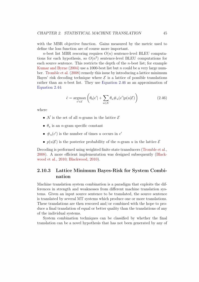
CHAPTER 2. STATISTICAL MACHINE TRANSLATION 45
with the MBR objective function. Gains measured by the metric used todefine the loss function are of course more important.
n-best list MBR rescoring requires O(n) sentence-level BLEU computa-tions for each hypothesis, so O(n2) sentence-level BLEU computations foreach source sentence. This restricts the depth of the n-best list; for exampleKumar and Byrne (2004) use a 1000-best list but n could be a very large num-ber. Tromble et al. (2008) remedy this issue by introducing a lattice minimumBayes’ risk decoding technique where E is a lattice of possible translationsrather than an n-best list. They use Equation 2.46 as an approximation ofEquation 2.44:
e = argmaxe′∈E
(θ0|e′|+
∑u∈N
θu#u(e′)p(u|E)
)(2.46)
where
• N is the set of all n-grams in the lattice E
• θu is an n-gram specific constant
• #u(e′) is the number of times u occurs in e′
• p(u|E) is the posterior probability of the n-gram u in the lattice E
Decoding is performed using weighted finite state transducers (Tromble et al.,2008). A more efficient implementation was designed subsequently (Black-wood et al., 2010; Blackwood, 2010).
2.10.3 Lattice Minimum Bayes-Risk for System Combi-nation
Machine translation system combination is a paradigm that exploits the dif-ferences in strength and weaknesses from different machine translation sys-tems. Given an input source sentence to be translated, the source sentenceis translated by several MT systems which produce one or more translations.These translations are then rescored and/or combined with the hope to pro-duce a final translation of equal or better quality than the translations of anyof the individual systems.
System combination techniques can be classified by whether the finaltranslation can be a novel hypothesis that has not been generated by any of
CHAPTER 2. STATISTICAL MACHINE TRANSLATION 46
the individual systems. System combination techniques that can generate anovel hypothesis usually employ consensus network decoding (Fiscus, 1997).In consensus network decoding for MT, n-best lists obtained from individualsystems are aligned to a reference, e.g. the MBR hypothesis, then the finalhypothesis is obtained by majority voting. In practice, it is difficult to applyconsensus network decoding to deep n-best lists or to lattices because of theexpensive alignment operation.
Another broad class of system combination techniques that do not gener-ate novel hypotheses include n-best list rescoring as well as lattice rescoringtechniques. Blackwood (2010) argues that one possible advantage over con-sensus network decoding is that fluency is more likely to be preserved andthat it is possible to exploit larger hypothesis spaces coming from individualsystems.
It is possible to extend the lattice Minimum Bayes-Risk decoding strategypresented in Section 2.10.2 for system combination. We consider two systemsthat produce two translation lattices E1 and E2. The statistics p(u|E) arecomputed by interpolation. The decoding equation becomes:
e = argmaxe′∈E1∪E2
(θ0|e′|+
∑u∈N1∪N2
θu#u(e′)(λ1p(u|E1) + λ2p(u|E2))
)(2.47)
The weights (λ1, λ2) are such that λ1 + λ2 = 1 and are tuned for BLEU ona development set.
Chapter 3
Data Structures for HierarchicalPhrase-Based TranslationGrammars
We have seen in Chapter 2 that the main components of an SMT systemare the translation model and the language model. The translation model istrained on parallel text while the language model is typically trained on thetarget side of the parallel text and possibly additional monolingual targettext. It has been shown that increasing the amount of parallel text (Pinoet al., 2010) and increasing the amount of monolingual text (Brants et al.,2007) is beneficial for translation quality.
Monolingual and parallel text availability and distributed computing tech-niques have allowed SMT researchers to build ever larger language modelsand translation models, based on very large amounts of data. However, de-coders need to be able to retrieve information, such as n-gram conditionalprobabilities or translation grammar rules, efficiently from these models tobe able to translate an input sentence or a set of input sentences in a rea-sonable amount of time. For online systems such as the commercial systemsmentioned in Chapter 1, translation even needs to be carried out in real time,i.e. for example with a speed of 2000 words translated per minute.
Therefore SMT models need to be stored in a data structure that supportsefficient querying and is scalable. We introduce a solution that addressesthese two requirements and that has the advantage that it reuses an existingframework in order to ease the implementation. We store translation models
47

CHAPTER 3. DATA STRUCTURES FOR HIERO GRAMMARS 48
0
1000
2000
3000
4000
5000
6000
7000
2006 2007 2008 2009 2010 2011 2012 2013
Num
ber
of m
illio
ns o
f tok
ens
Year
EN parallel dataEN monolingual data
Figure 3.1: Number of English tokens (in millions) in parallel and monolin-gual data available for the WMT French-English constrained track transla-tion shared task for the years 2006 to 2013.
as a set of key-value pairs in an HFile1. We apply this strategy in order toretrieve relevant rules from a hierarchical phrase-based grammar at the testset level. We compare our approach to alternative strategies and show thatour approach offers competitive performance in terms of speed, memory andsimplicity (Pino et al., 2012). We have made software written for this workavailable online.2
3.1 IntroductionCurrent machine translation research is characterised by increasing amountsof available data. For example, Figure 3.1 shows that for the WMT machinetranslation workshop (Bojar et al., 2013) French-English constrained tracktranslation shared task, the English side of parallel data has increased from13.8M tokens in 2006 to 1012.7M tokens in 2013, and that available Englishmonolingual data has increased from 27.5M tokens to 6852.7M tokens overthe same period. Along with growing amounts of data, the use of more power-
1 http://hbase.apache.org2 https://github.com/jmp84/ruleXtract (branch PBML-2012)

CHAPTER 3. DATA STRUCTURES FOR HIERO GRAMMARS 49
ful computers and distributed computing models such as MapReduce (Deanand Ghemawat, 2008; Lin and Dyer, 2010) has enabled machine translationresearchers to build larger statistical machine translation models. MapRe-duce has thus been applied to various steps of the translation pipeline: wordalignment (Dyer et al., 2008), translation model building (Dyer et al., 2008)and language modelling (Brants et al., 2007). We review these applicationsof MapReduce in more detail in Section 3.2. The challenge is to find effectivemodelling techniques that can be implemented in the MapReduce framework.
However, once SMT models such as language models and translationgrammars are built, either with MapReduce or some other method, the mod-els must be made usable by translation decoders, which only need a fractionof the information contained in those models to be able to translate an inputsource sentence or a set of input source sentences. For example, in translationfrom French to English with a phrase-based model (see Section 2.5), given aninput sentence Salut toi, we only need to know the translation probabilitiesthe translation model assigns to translations of the words Salut and toi andto translations of the phrase Salut toi. Similarly, given a test set, a decoderonly needs to retrieve the rules whose source side matches part of one ofthe source sentences in the test set to be able to generate hypotheses. Withlarge models, simply retrieving relevant rules together with their translationprobabilities becomes a challenge.
In the system described by Iglesias et al. (2009b), given a training parallelcorpus, rules are extracted and target phrases and hierarchical phrases withcounts are stored on disk. Then, given an input test set, rules are extractedfrom the parallel corpus a second time. Only rules relevant to the test set areretained: source sides of phrase-based rules have to match an n-gram fromthe test set and consecutive terminals in source sides of hierarchical rulesalso have to match an n-gram from the test set. As a consequence, somehierarchical rules are never used in decoding. Source sides and rules togetherwith their counts are kept in memory using hash map datastructures, targetsides with counts are loaded from disk as precomputed in the first step, sothat source-to-target and target-to-source probabilities can be computed.
This method becomes progressively slower with larger amounts of databecause it requires extracting rules from the training parallel corpus andrecomputing translation probabilities each time we translate a new test setor a new sentence. We would like to improve on this design for more rapidexperimentation. We also would like to use a computing infrastructure that

CHAPTER 3. DATA STRUCTURES FOR HIERO GRAMMARS 50
requires minimal maintenance. For example, HBase3, the open source non-relational database implementation of BigTable (Chang et al., 2008), hasbeen applied to the use of distributed language models (Yu, 2008). Rulefiltering, i.e. the retrieval of rules relevant to the translation of a test set ora sentence, is an essential step in our pipeline that can be a bottleneck. Ourgoal is to reduce its processing time from several hours to a few minutes.
In this chapter, we address the problem of retrieving relevant rules withtheir translation probabilities. We report on investigations into storing themodel in the HFile data structure. To our knowledge, this is the first de-tailed proposed implementation of translation model storage and filteringusing HFile data structures. We find that this approach offers a good com-promise between speed, performance and ease of implementation. The in-frastructure necessary for filtering is lightweight and requires the use of onlyone machine. We will apply this approach to test set rule filtering prior todecoding. We will discuss alternative strategies as well as their strengthsand weaknesses in terms of speed and memory usage. In Section 3.2, wewill review approaches that have been used for model building and modelfiltering. The HFile data structure that is used to store models will be pre-sented in Section 3.3. In Section 3.4, we detail our custom implementationof rule extraction and translation model estimation using MapReduce. Ourmethod and alternative strategies for rule filtering are compared empiricallyin Section 3.5. We conclude in Section 3.6.
3.2 Related WorkIn this section, we review applications of MapReduce to the translationpipeline as well as techniques for storing and retrieving from SMT models.
3.2.1 Applications of MapReduce to SMT
Brants et al. (2007) introduce a new smoothing method called Stupid Backoff(see Section 2.7.4). The Stupid Backoff smoothing scheme is recalled in
3 http://hbase.apache.org
CHAPTER 3. DATA STRUCTURES FOR HIERO GRAMMARS 51
Equation 3.1:
pstupid backoff(wi | wi−1i−n+1) =
c(wi
i−n+1)
c(wi−1i−n+1)
if c(wii−n+1) > 0
α pstupid backoff(wi | wi−1i−n+2) if c(wi
i−n+1) = 0
(3.1)With respect to the traditional backoff scheme, the Stupid Backoff schemeuses no discounting and simply uses relative frequency for the non backed-offscore and the backed-off score scaling parameter is independent of the n-gram history. Therefore this scheme does not define a conditional probabilitydistribution over a word given its history.
The Stupid Backoff language model building and application fit the MapRe-duce framework well. The input to language model building is a large mono-lingual corpus. The first step is to build a vocabulary. This is done with thecanonical example of word counting with MapReduce. Counts are neededin order to remove words occurring less than a threshold from the vocabu-lary. The second step is to obtain n-grams and their count. This is doneagain with MapReduce, and the map and reduce functions are analogous tothe ones defined for word counting but this time unigrams are replaced byn-grams. For n-gram counting, the partition, or sharding, function hasheson the first two words of each n-gram. In addition, unigram counts and thetotal size of the corpus is available in each partition, i.e. to each reducer.This allows relative frequencies to be computed. Brants et al. (2007) alsodemonstrate that for large amounts of monolingual data, i.e. above 10 bil-lion tokens, Stupid Backoff smoothing and Kneser-Ney smoothing performcomparably. In addition, only Stupid Backoff smoothing can be scaled todatasets with more than 31 billion tokens. The scalability of Kneser-Neysmoothing has been improved in recent work (Heafield et al., 2013).4
Dyer et al. (2008) observe that translation model estimation has becomeprohibitive on a single core and that existing ad hoc parallelisation algo-rithms may be more fragile than using an existing framework such as theHadoop implementation of MapReduce.5 They provide solutions to wordalignment model estimation and translation rule extraction and estimationusing MapReduce and demonstrate the scalability of their method.
The convenience of the MapReduce framework for parallelisation has ledto the building of end-to-end toolkits for entire phrase-based (Gao and Vogel,
4 see also http://kheafield.com/code/kenlm/estimation/, Scalability section5 https://hadoop.apache.org/

CHAPTER 3. DATA STRUCTURES FOR HIERO GRAMMARS 52
2010) and hierarchical phrase-based models (Venugopal and Zollmann, 2009)for translation using the MapReduce framework.
3.2.2 SMT Models Storage and Retrieval Solutions
We now review techniques appearing in the literature that have been usedto store SMT models and to retrieve the information needed in translationfrom these models. SMT models are usually discrete probabilistic models andcan therefore be represented as a set of key-value pairs. To obtain relevantinformation from a model stored in a certain data structure, a set of keyscalled a query set is formed; each key in this query set is then sought in thatdatastructure. Strategies include:
• storing the model as a simple data structure in memory
• storing the model in a text file
• storing the model in more complicated data structures such as tries (Fred-kin, 1960) (in memory or disk)
• storing fractions of the entire model
• storing data as opposed to a precomputed model
• storing models in a distributed fashion
Each of these strategies is discussed below.In some cases, it may be possible to fit a model into RAM. In this case
the model can be stored as a memory associative array, such as a hash ta-ble. In-memory storage allows allows for faster query retrieval than on-diskstorage, however only smaller models will fit in memory. In-memory storagehas been used to store model parameters between iterations of expectation-maximisation for word alignment (Dyer et al., 2008; Lin and Dyer, 2010).
For larger models, the set of key-value pairs can be stored as a tablein a single text file on local disk. Values for keys in the query set can beretrieved by scanning through the entire file. For each key in the file, itsmembership is tested in the query set. This is the approach adopted in theJoshua 5.0 decoder (Post et al., 2013)6, which uses regular expressions or
6 Inferred from the decoder training scripts available at http://joshua-decoder.org/5.0/index.html.

CHAPTER 3. DATA STRUCTURES FOR HIERO GRAMMARS 53
n-grams to test membership (see Section 3.5.4). Venugopal and Zollmann(2009) use MapReduce to scan a file concurrently: the map function tests ifthe vocabulary of a rule matches the vocabulary of a test set.
The model can also be stored using a trie associative array (Fredkin,1960). A trie is a type of tree where each node represents a shared prefix of aset of keys represented by the child nodes. Each node only stores the prefix itrepresents. The keys are therefore compactly encoded in the structure of thetrie itself. Querying the trie is a O(log(n)) operation, where n is the numberof keys in the dataset. The trie may also be small enough to fit in physicalmemory to further reduce querying time. Zens and Ney (2007) use tries tostore a phrase-based grammar. All the source phrases are represented in a triestored on disk. Only relevant parts of the trie are loaded into memory whena source phrase is sought. Ganitkevitch et al. (2012) extend this approachto store hierarchical phrase-based grammars. Both source sides and targetsides are stored in a packed representation of a trie. Packed tries have alsobeen applied for storing language models (Pauls and Klein, 2011; Heafield,2011).
It is also possible to create a much smaller approximate version of themodel. Talbot and Osborne (2007a) represent a set of n-grams as a Bloomfilter (Bloom, 1970). They first use a standard Bloom filter to define a binaryfeature that indicates whether an n-gram was seen in a monolingual corpus.They also use a Bloom filter to encode n-grams together with quantisedcounts in order to define a multinomial feature, that is a feature with a finiteset of possible values—in this case the quantised values. Both these datastructures can substantially reduce the disk space and memory usage withrespect to lossless representations of language models. However, they allowfalse positives for n-gram membership queries and overestimates of n-gramquantised counts. The authors demonstrate that the features they introduceare useful in translation, despite this lack of exactness. In a related pub-lication (Talbot and Osborne, 2007b), the authors demonstrate how thesetechniques can be used as a replacement to represent a smoothed languagemodel. Talbot and Brants (2008) use a Bloomier filter (Chazelle et al., 2004)to represent n-grams and necessary statistics such as probabilities and back-off weights. Unlike Bloom filters that only support Boolean characteristicfunctions on a set, Bloomier filters support arbitrary functions, in this case amapping between an n-gram and its statistics. False positives can still occurbut for true positives, correct statistics are retrieved.

CHAPTER 3. DATA STRUCTURES FOR HIERO GRAMMARS 54
Guthrie and Hepple (2010) propose an extension to previous work onrandomised language models (Talbot and Osborne, 2007b) which preventsthe random corruption of model parameters but does not stop the randomassignment of parameters to unseen n-grams. Levenberg and Osborne (2009)extend randomised language models to stream-based language models. An-other way of building a smaller approximate version of a model is to retainitems with high frequency counts from a stream of data (Manku and Mot-wani, 2002). This technique has been applied to language modelling (Goyalet al., 2009) and translation rule extraction (Przywara and Bojar, 2011).
Instead of doing some precomputation on a dataset, it is possible to com-pute the sufficient statistics at query time using a suffix array (Manber andMyers, 1990), so that the model can be estimated only when needed. A suf-fix array is a sequence of pointers to each suffix in a training corpus. Thesequence is sorted with respect to the lexicographic order of the referencedsuffixes. Suffix arrays have been used for computing statistics for languagemodels (Zhang and Vogel, 2006), phrase-based systems (Callison-Burch et al.,2005; Zhang and Vogel, 2005), and hierarchical phrase-based systems (Lopez,2007). Callison-Burch et al. (2005) store both the source side and the targetside of a parallel corpus in two suffix arrays. They also maintain an indexbetween a position in the source or target side of the corpus and the sentencenumber. During decoding, all occurrences of a source phrase are located inthe suffix array representing the source side of the corpus. This producesa source marginal count. For each of these occurrences, the correspondingsentence pair and word alignment are retrieved and rules are extracted. Thisproduces a rule count, which is normalised with the source marginal count toproduce a source-to-target probability. Lopez (2007) extends this approachto address the grammar extraction and estimation of hierarchical rules. Notethat the use of suffix arrays for translation model estimation only supportsthe computation of source-to-target probabilities.
Finally, some approaches store language models in a distributed fashion.We saw in Section 3.2.1 how a Stupid Backoff language model can be built.After relative frequencies have been computed, another partition functionthat hashes on the last two words of an n-gram is applied so that backoffoperations can be done within the same partition. At decoding time, thedecoder architecture is modified in order to request a batch of n-grams ratherthan a single n-gram. The Stupid Backoff language model building can bescaled to a corpus of 2 trillion tokens and the language model distributedapplication can be made real time.

CHAPTER 3. DATA STRUCTURES FOR HIERO GRAMMARS 55
Zhang et al. (2006) propose a distributed large language model backedby suffix arrays. HBase has also been used to build a distributed languageinfrastructure (Yu, 2008). The method we propose to use is closely related tothe latter but we use a more lightweight infrastructure than HBase. In addi-tion, it is also possible to apply our method to language model querying (Pinoet al., 2012), which demonstrates the flexibility of the infrastructure.
Note that there are many alternative solutions to HBase/HFile for storageof a large number of key-value pairs, such as Berkeley DB7 or Cassandra8.The purpose of this chapter is not to compare these alternatives but rather tocompare existing solutions employed in the machine translation communityto one of these solutions.
3.3 HFile DescriptionWe now describe the data structure we use to store models and we reviewrelevant features to the design of our system. To store a model representedas key-value pairs, we use the HFile file format,9 which is an open sourcereimplementation of the SSTable file format (Chang et al., 2008). The HFileformat is a lookup table with key and value columns. The entries are freeto be an arbitrary string of bytes of any length. The table is sorted lexico-graphically by the key byte string for efficient record retrieval by key.
3.3.1 HFile Internal Structure
High Level Structure As can be seen in Figure 3.2, the HFile internalstructure is divided into blocks. There are various types of block, dependingon the kind of information a block contains. In order to distinguish blocktypes, the first 8 bytes of a block will indicate its type. The blocks aregrouped into three parts. The first part (top) is organised into data blocksinterleaved with leaf data index blocks and Bloom blocks. The second part(middle) consists of intermediate data index blocks. The third part (bottom)consists of metadata: root data index blocks, a file information block and aBloom filter index block.
7 https://oss.oracle.com/berkeley-db.html8 http://cassandra.apache.org9 http://hbase.apache.org

CHAPTER 3. DATA STRUCTURES FOR HIERO GRAMMARS 56
Data Block...Leaf Data Index Block / Bloom Block...Data Block...Leaf Data Index Block / Bloom Block...Data BlockIntermediate Data Index BlocksRoot Data Index BlocksFile Info BlockBloom Filter Index Block
Figure 3.2: HFile internal structure.11 The structure is divided into threeparts. In the first part, data blocks are interspersed with leaf data indexblocks and Bloom blocks. The second part contains intermediate data indexblocks. The third part consists of metadata: root data index blocks, fileformat information and a Bloom filter index block.
Index Blocks The root data index blocks map keys to their relevant in-termediate data index block, indicated by an offset. In turn, an intermediatedata index block maps keys to their relevant leaf data index block, againindicated by an offset. Finally, a leaf data index block maps keys to theirrelevant data block, still indicated by an offset. The same mechanism is em-ployed for the Bloom filter. The Bloom filter index block maps keys to theirrelevant Bloom block.
Block Size Configuration The block size is configurable, with a defaultsize of 64KB. Note that HFile blocks are not to be confused with HadoopDistributed File System (HDFS) blocks whose default size is 64MB.
Block Compression The HFile format allows for the blocks to be com-pressed. The choice of compression codec is selected when the file is created.We choose the GZip compression codec (Deutsch and Gailly, 1996) for allour experiments.

CHAPTER 3. DATA STRUCTURES FOR HIERO GRAMMARS 57
3.3.2 Record Retrieval
When the HFile is opened for reading, the root data index blocks are loadedinto memory. To retrieve a value from the HFile given a key, the appropriateintermediate index block is located by a binary search through the root dataindex. Binary searches are conducted on the intermediate and leaf indexblocks to identify the data block that contains the key. The identified datablock is then loaded off the disk into memory and the key-value record isretrieved by scanning the data block sequentially.
3.3.3 Bloom Filter Optimisation for Query Retrieval
It is possible to query for a key that is not contained in the HFile. This veryfrequently happens in translation because of language data sparsity: in ourcase, because keys are n-grams of terminals and nonterminals, the number ofpossible keys is exponential in the size of the vocabulary, and many of thesewill not have been observed in any rule extracted from training data.
Querying the existence of a key is expensive as it involves all the op-erations described in Section 3.3.2: loading and binary searching the rootdata index, loading and binary searching an intermediate data index block,loading and binary searching a leaf data index block and finally loading andscanning a data block.
For fast existence check queries, the HFile format allows the inclusion ofan optional Bloom filter (Bloom, 1970). A Bloom filter provides a probabilis-tic, memory efficient representation of the key set with a O(1) membershiptest operation. The Bloom filter may provide a false positive, but never afalse negative, for existence of a key in the HFile. Therefore, it is safe to usein our setting as some keys will be looked up in the HFile even though theyare not present, but the situation where keys that are in the HFile are notlooked up will not happen.
For a large HFile, the Bloom filter may also be very large. Therefore theBloom filter is also organised into blocks called Bloom blocks. Each blockcontains a smaller Bloom filter that covers a range of keys in the HFile.Similar to the root data index, a Bloom index is constructed. To check forthe existence of a key, a binary search is conducted on the Bloom index, therelevant Bloom block is loaded, and the membership test performed.
11 After http://hbase.apache.org/book/book.html (simplified)

CHAPTER 3. DATA STRUCTURES FOR HIERO GRAMMARS 58
Unlike work on Bloom filter language models (Talbot and Osborne, 2007a,b),this filter only tests the existence of a key and does not return any statisticsfrom the value. If a membership test is positive, a usual key search will stillbe carried out. During the execution of a query, two keys may reference thesame index or Bloom blocks. To prevent these blocks from being repeatedlyloaded from disk, the blocks are cached after reading.
3.3.4 Local Disk Optimisation
The HFile format is designed to be used with HDFS, a distributed file systembased on the Google File System (Ghemawat et al., 2003). Large files aresplit into HDFS blocks that are stored on many nodes in a cluster. However,the HFile format can also be used completely independently of HDFS. Ifits size is smaller than local disk space, the entire HFile can be stored onthe local disk of one machine and accessed through the machine’s local filesystem. We report in Section 3.5 that using local disk is faster than usingHDFS.
3.3.5 Query sorting optimisation
Prior to HFile lookup, we sort keys in the query set lexicographically. If twokeys in the set of queries are contained in the same block, then the block isonly loaded once. In addition, the computer hardware and operating systemallow further automatic improvements to the query execution. Examplesof these automatic improvements include reduced disk seek time, cachingdata from disk by the operating system,12 or CPU caching data from mainmemory (Patterson and Hennessy, 2009).
3.4 Hierarchical Rule Extraction with MapRe-duce
In the previous section, we have described the HFile format. We will usethis format to store a translation grammar. In this section, we describe howwe generate this grammar and produce the HFile that represents the gram-mar. We describe a MapReduce implementation of hierarchical grammar
12 The Linux Documentation Project, The File System, http://tldp.org
CHAPTER 3. DATA STRUCTURES FOR HIERO GRAMMARS 59
extraction and estimation. The implementation is an extension of Method 3described by Dyer et al. (2008), which was originally developed to estimatetranslation probabilities for phrase-based models.
MapReduce (Dean and Ghemawat, 2008) is a framework designed forprocessing large amounts of data in a distributed fashion on a computercluster. In this framework, the programmer needs to implement a functioncalled map and a function called reduce. The map function is defined inEquation 3.2:
map : (k1, v1) 7−→ [(k2, v2)] (3.2)
where (k1, v1) is a key-value pair and [(k2, v2)] is a list of key-value pairs.We use the [ ] notation to denote a list. Keys and values are arbitrary bytesequences. As the key-value pairs (k2, v2) are computed by the map function,the MapReduce framework groups all values v2 by key k2 in order to providean input (k2, [v2]) to the reduce function, defined in Equation 3.3:
reduce : (k2, [v2]) 7−→ [(k3, v3)] (3.3)
The input to the reduce function is a key and a list of values. The reducefunction generates a list of key-value pairs.
Using this notation, we can describe the grammar extraction and estima-tion as a series of MapReduce jobs, summarised in Figure 3.3. This architec-ture is similar to the one described in the original publication (Dyer et al.,2008). For source-to-target and target-to-source probability computation,we used Method 3 described in that publication, which was reported to befaster than other methods. Keeping each feature computation as a separateMapReduce job makes the integration of a new feature more convenient.
3.4.1 Rule Extraction
The first step in grammar extraction and estimation is rule extraction. Forthis step, v1 represents a sentence pair together with a word alignment andk1 contains metadata about the parallel corpus such as what collection thesentence pair comes from. This kind of information is useful for domainadaptation as demonstrated in Section 5.5. The map function simply extractshierarchical rules for that sentence pair and outputs the rules. k2 is a ruleand v2 contains the metadata from k1. For rule extraction, there is no reducestep. Equation 3.4 illustrates the map function for rule extraction:
map : (newswire, (f , e,a)) 7−→ [(r1, newswire), (r2, newswire), ...] (3.4)

CHAPTER 3. DATA STRUCTURES FOR HIERO GRAMMARS 60
..k1 : metadatak2 : word-aligned sentence pair
.
Rule Extraction (see Section 2.6.4)map : extract rulesreduce : none
.
k1 : rulek2 : metadata
.
Source-to-target Probabilitymap : output (src, (trg, 1))reduce : sum trg counts, normalise
.
Target-to-source Probabilitymap : output (trg, (src, 1))reduce : sum src counts, normalise
.
k1 : rulek2 : source-to-target pr
.
k1 : rulek2 : target-to-source pr
.
Mergemap : output (src, (trg, feature))reduce : output (src, list of trg and features)
.
k1 : srck2 : list of trg and features
Figure 3.3: Translation grammar extraction and estimation pipeline as a se-ries of MapReduce jobs. Ellipses represent (intermediate) input/output ofMapReduce jobs. Rectangles represent MapReduce jobs. Source, target andprobability are abbreviated into src, trg and pr. Rules are first extracted,then the source-to-target and target-to-source translation models are esti-mated. Finally, the features, i.e. the translation models, are merged and thefinal output has rules sources as keys and lists of targets with features asvalues.

CHAPTER 3. DATA STRUCTURES FOR HIERO GRAMMARS 61
3.4.2 Corpus-Level Feature Computation
Rule extraction is followed by several MapReduce jobs that are run simulta-neously in order to compute corpus-level features. Corpus-level features arefeatures related to each rule and the computation of which requires lookingat the entire set of extracted rules. In this description, we only considersource-to-target and target-to-source probabilities, but many other corpus-level features are possible, for example features that relate to the word align-ment from which rules were extracted. We use the metadata stored in theoutput of the extraction job in order to compute collection specific proba-bilities. Collection specific probabilities are probabilities computed over aspecific subset of the training corpus. The metadata indicates whether a rulewas extracted from that specific subset.
Let us consider first the collection-specific source-to-target probabilitycomputation. The input to the map function is the output of the extractionjob, that is a rule together with metadata. The map function checks thatthe rule comes from the collection we are interested in and if so, outputs thesource of the rule as a key k2 and the target of the rule together with a countof one as a value v2. Targets (and counts) corresponding to the same sourceare grouped together by the MapReduce framework. The input to the reducefunction is a source (k2) and a list of targets with counts ([v2]). The reducefunction aggregates the counts for the distinct targets and then normalisesthose counts with the total count corresponding to the source k2. The outputof the reduce function is a list of pairs (rule, probability).
The target-to-source probability computation is very similar. Apart frominverting the role played by source and target, the map and reduce functionalso need to change the rule format for rules that invert the order of nonter-minals in the source and the target, for example X→〈X1aX2,X2bX1〉. Forthis type of rule, the map function has to invert the order of nonterminalsin both the source and target so that probabilities are computed correctly.For example, the map function will output the target of the rule written asX1bX2 and the source of the rule written as X2aX1. The reduce function willrestore the original notation.
We have described the computation of collection specific translation prob-abilities. The source-to-target and target-to-source probabilities over the en-tire corpus are computed in an identical manner with the collection simplybeing the entire corpus. Figure 3.3 illustrates only two corpus-level fea-tures, however, in practice, more features are computed: source-to-target
CHAPTER 3. DATA STRUCTURES FOR HIERO GRAMMARS 62
and target-to-source probability for each collection and for the entire paralleltext, as well as lexical features (see Section 2.6.5).
3.4.3 Feature Merging
Once all MapReduce features have been computed, a MapReduce job thatmerges the features is called. The input key k1 to the map function is arule and the input value v1 is a feature. The map function outputs thesource of the rule as a key k2 and the target of the rule together with thefeature as value v2. Targets and features corresponding to the same sourceare grouped together by the MapReduce framework. The input to the reducefunction is a source (k2) and a list of targets with features ([v2]). The reducefunction simply merges the features for identical targets. The output key k3is the source k2 and the output value v3 is a list of targets with all computedfeatures.
The output of this merging job is converted to an HFile format. Becausethe keys in the HFile format need to be sorted, we also want the output of themerging job to be sorted by key. One way to achieve this is to specify only onereducer for the job but this solution is very slow because only one core will beused for the reduce step. A better way is to use a TotalOrderPartitioner. Wefirst use a small amount of data so that it may be feasible to carry out ruleextraction with only one reducer in the merge step. We use the output of thissmall scale extraction as input to an InputSampler. The sampler will generatea partition file for the partitioner. The use of a TotalOrderPartitioner willguarantee that all keys are sorted after the reduce step.
3.5 Hierarchical Rule Filtering for TranslationIn the previous section, we have described how to obtain an HFile that rep-resents a hierarchical translation grammar. We will now describe how thisdatastructure can be used to retrieve rules for a given test set efficiently.We describe our system called ruleXtract, and compare it to other methodsthrough time and memory measurements.

CHAPTER 3. DATA STRUCTURES FOR HIERO GRAMMARS 63
3.5.1 Task Description
Given a test set, defined as a set of sentences to be translated, and a hier-archical phrase-based translation grammar, we would like to retrieve all therelevant rules from the model. A phrase-based rule in the HFile is relevantif its source is a subsequence of a sentence in the test set. A hierarchicalrule in the HFile is relevant if its source, where nonterminals are instantiatedinto terminals, is a subsequence of a sentence in the test set. For exam-ple, with a test set containing one sentence Salut toi, the phrase-based ruleswith sources Salut, toi, Salut toi are relevant and the hierarchical rules withsources Salut X and X toi are relevant, because instantiating Salut X intoSalut toi produces a subsequence of the test sentence and similarly for X toi.
3.5.2 HFile for Hierarchical Phrase-Based Grammars
Given a test set and an HFile storing a hierarchical phrase-based grammar,we first generate queries from the test set, then retrieve relevant rules alongwith their corpus-level features from the HFile. To generate queries, we havea set of allowed source patterns and instantiate these patterns against the testset. Rule patterns were defined in Section 2.6.2. A source pattern is simplythe source side of a rule pattern. Here, we briefly redefine source patterns. Asource pattern is a regular expression that matches the source side of a rule.For example, the pattern Σ+X, with Σ the source vocabulary, represents arule source side containing a sequence of terminals followed by the nontermi-nal X. If the input sentence is Salut a toi, the pattern will be instantiated asSalut X, Salut a X and a X. We impose the following constraints on sourcepattern instantiation where the first four relate to constraints in extractionand the last one relates to a decoding constraint:
• smax: maximum number of terminals for phrase-based rules.
• smax elements: maximum number of terminals and nonterminals.
• smax terminals: maximum number of consecutive terminals for hierarchi-cal rules.
• smax NT: maximum nonterminal span in a hierarchical rule.
• smax span: maximum span for the rule. This constraint is not to beconfused with the previous smax NT constraint. While smax NT represents

CHAPTER 3. DATA STRUCTURES FOR HIERO GRAMMARS 64
the maximum span of a nonterminal on the right hand side of a rule,smax span represents the maximum span of an entire rule, or alternativelythe maximum span of the nonterminal on the left hand side of the rule.Because the latter constraint is enforced by the decoder, we also enforceit in source pattern instantiation so that rules that will never be usedby the decoder are not generated.
The source pattern instances are then sorted for more efficient HFile lookup(see Section 3.3.5). Each query is then looked up in the HFile and if present,an HFile record is retrieved. We now compare our approach to similar ap-proaches whose aim is to obtain rules which are relevant to a test set.
3.5.3 Suffix Arrays for Hierarchical Phrase-Based Gram-mars
One alternative strategy for building a set specific grammar is to use suf-fix arrays introduced in Section 3.2. We use the cdec software (Dyer et al.,2010) implementation of suffix arrays for hierarchical phrase-based rule ex-traction. The cdec implementation is based on earlier work (Lopez, 2007)which extends suffix array based rule extraction from phrase-based systemto hierarchical phrase-based systems (see again Section 3.2).
Given a test set, a set of source pattern instances is generated similarly towhat is done for ruleXtract. These source pattern instances are then soughtin a suffix array compiled from the source side of a parallel corpus. Rules areextracted using the word alignment, and source-to-target probabilities arethen computed as described in Section 3.2.
3.5.4 Text File Representation of Hierarchical Phrase-Based Grammars
We now describe the Joshua decoder (Weese et al., 2011) implementation forstoring and retrieving from a translation model. The first implementationvariant, which we call Joshua, stores the translation model in a text file.Given a test set, each word in the test set vocabulary is mapped to the listof sentences in which it appears. Then, each rule in the translation model iscompiled to a regular expression, and each sentence that contains at least avocabulary word of the rule is matched against this regular expression. If atleast one match is successful, the rule is retained.

CHAPTER 3. DATA STRUCTURES FOR HIERO GRAMMARS 65
A faster version is provided that matches consecutive terminals in thesource side of a rule to the set of n-grams extracted from the test set. Wecall this version Joshua Fast. A parallel version also exists that chunks thegrammar file and distributes each chunk processing as a separate process ona cluster running Sun Grid Engine (Gentzsch, 2001). We call this versionJoshua Parallel. The parallel version using the faster matching algorithm iscalled Joshua Fast Parallel.
3.5.5 Experimental Design
In this section, we describe our experimental setup in terms of data andvarious configurations for grammar extraction, grammar filtering and timeand memory measurements.
Parallel Text We use a small parallel corpus of 750,950 word-aligned sen-tence pairs and a larger corpus of 9,221,421 word-aligned sentence pairs fromthe NIST’12 Chinese-English evaluation, in order to investigate how systemsperform with varying amounts of parallel text and whether those systems arerobust when dealing with larger data sets.
Grammar Extraction From the parallel corpora, we extract hierarchicalgrammars with the source-to-target probability feature only. This is done be-cause we do not want feature computation to introduce variability in timingresults when comparing different strategies and software implementations.In addition, not all systems can generate the same set of features. For exam-ple, the suffix array implementation of rule extraction is not able to generatetarget-to-source probabilities. Note that in practice for translation decod-ing, given a vector of parameters, we could simply replace multiple featuresin the translation model by a single value representing the dot product ofthe features with the parameter vector. However, we need to keep separatefeature values for optimisation (see Section 2.8.2).
The rule extraction constraints described in Section 3.5.2 are set to amaximum source phrase length smax of 9, a maximum source element (termi-nal and nonterminal) length smax elements of 5, a maximum number of sourceconsecutive terminals smax terminals of 5 and a maximum source nonterminalspan smax NT of 10. These settings are standard in all our translation systemsand give competitive performance in terms of translation quality.

CHAPTER 3. DATA STRUCTURES FOR HIERO GRAMMARS 66
With these settings, the small grammar contains approximately 60M ruleswhile the larger grammar contains approximately 726M rules. The grammarswe obtain are converted to the Joshua format in order to be able to filterthem with the Joshua decoder. We do not generate a hierarchical grammarwith Joshua simply because we want to compare the performance of ruleretrieval from the same grammar.
Grammar filtering For ruleXtract, we use the following constraints forsource pattern instantiation: the maximum source phrase length smax isset to 9, the maximum source element (terminal and nonterminal) lengthsmax elements is set to 5, the maximum number of source consecutive terminalssmax terminals is set to 5, the maximum source nonterminal span smax NT isset to ∞ and the maximum rule span smax span is set to ∞. The first threeconstraints are standard in all our translation systems. We use the value∞ for smax NT and smax span so that the number of rules obtained after fil-tering is identical between ruleXtract and Joshua. Thus, time and memorymeasurements are comparable.
Measurements We report time measurements for query processing andquery retrieval and the total time used to obtain a set specific rule file fora test set of 1755 Chinese sentences and 51008 tokens. We also report peakmemory usage. For ruleXtract, query processing involves generating sourcepattern instances and sorting them according to the HFile sorting order. Ifwe use a Bloom filter, it also involves pre-filtering the queries with the Bloomfilter. Query retrieval involves HFile lookup. For the Joshua configurations,query processing involves indexing the test set and generating test set n-grams and query retrieval involves regular expression matching.
For the Joshua Parallel configurations, we use 110 jobs for the largergrammar on a cluster of 9 machines. For this latter configuration, we reportthe maximum time spent on a job (not the sum) and the maximum memoryusage by a job.
Hardware configuration the machine used for query processing has 94GBof memory and an Intel Xeon X5650 CPU. The distributed file system ishosted on the querying machine and other machines with the same specifi-cation, which are used to generate the HFile.

CHAPTER 3. DATA STRUCTURES FOR HIERO GRAMMARS 67
Our experimental setup was designed for accurate comparisons betweenalternative strategies for grammar filtering. In practice, an end-to-end trans-lation system need not use this exact setup. For example the grammarextracted by Joshua is in general smaller than the grammar extracted byruleXtract because Joshua includes target side constraints. On the otherhand, ruleXtract uses threshold cutoffs, such as a minimum source-to-targettranslation probability, in order to reduce the size of the test set specificgrammar.
3.5.6 Results and Discussion
Results are summarised in Table 3.1, from which we can draw the followingobservations:
Speed The Total Time column shows that ruleXtract is competitive withalternative strategies in terms of speed.
Memory The Peak Memory column shows that both ruleXtract and Joshuaare memory hungry, with a usage of up to 40GB. In the case of ruleXtract,this is because we keep all source pattern instances for all test set sentencesare kept in memory. In the case of Joshua, this is due to a caching optimisa-tion: rule source sides that have already been considered relevant to the testset are stored in a hash map.
Local disk optimisation Comparing HDFS and Local rows (row 1 vs.row 3, row 2 vs. row 4, row 7 vs. row 9, row 8 vs. row 10), we can see thatusing the local filesystem as opposed to HDFS gives a small decrease in queryretrieval time, which becomes more substantial for the larger grammar. Thisis because when the HFile is stored on HDFS, it is composed of several HDFSblocks that can be located on different data nodes. Since the HFile size issmaller than the disk space on each data node, it is preferable to store theHFile on local disk. However, because the HFile was generated on HDFSthrough a MapReduce job, this requires copying or moving the HFile fromthe HDFS file system to the local disk file system prior to running grammarretrieval.

CHAPTER 3. DATA STRUCTURES FOR HIERO GRAMMARS 68
Small GrammarRow System Query Query Total Peak # Rules
Processing Retrieval Time Memory1 ruleXtract 9m1s 7m36s 16m40s 40.8G 6435124
HDFS2 ruleXtract 8m57s 2m16s 11m15s 39.9G 6435124
Bloom, HDFS3 ruleXtract 8m54s 7m33s 16m30s 40.4G 6435124
Local4 ruleXtract 8m50s 2m19s 11m11s 38.8G 6435124
Bloom, Local5 Joshua 0.9s 29m51s 29m54s 42.2G 64351246 Joshua 0.9s 7m25s 7m28s 40.1G 7493178
FastLarge Grammar
Row System Query Query Total Peak # RulesProcessing Retrieval Time Memory
7 ruleXtract 8m56s 22m18s 31m17s 42.2G 47978228HDFS
8 ruleXtract 9m12 15m33s 24m49s 40.7G 47978228Bloom, HDFS
9 ruleXtract 8m55s 21m3s 30m1s 41.6G 47978228Local
10 ruleXtract 9m0s 14m43s 23m46s 40.6G 47978228Bloom, Local
11 Joshua 0.9s out of out of out of out ofmemory memory memory memory
12 Joshua 0.9s out of out of out of out ofFast memory memory memory memory
13 Joshua 0.9s 537m10s 537m11s 10.1G 47978228No Cache
14 Joshua 0.9s 78m53s 78m54s 10.1G 83339443Fast No Cache
15 Joshua total time for slowest job: 43m36s 4G 47978228Parallel
16 Joshua total time for slowest job: 44m29s 4G 83339443Fast Parallel
Table 3.1: Time and memory measurements for rule filtering with differ-ent strategies for a small and a large grammar. Various configurations forruleXtract and Joshua are compared for time and memory usage. The fastconfiguration for Joshua filters rules by matching consecutive terminals totest set n-grams, which explains that the number of rules obtained is higherthan in all other configurations. This also means that some filtered rulesare never used in decoding. Measurements were carried out twice for eachcondition and the second run was recorded. Thus, measurements reportedtake advantage of operating system caching.
CHAPTER 3. DATA STRUCTURES FOR HIERO GRAMMARS 69
Bloom filter optimisation Comparing rows with and without Bloom(row 1 vs. row 2, row 3 vs. row 4, row 7 vs. row 8 and row 9 vs. row 10), wecan see that the use of a Bloom filter gives an important decrease in queryretrieval time. This is due to the fact that the number of source pattern in-stances queries is 31,552,746 and after Bloom filtering, the number of queriesis 1,146,554 for the small grammar and 2,309,680 for the larger grammar,reducing the number of time consuming HFile lookups respectively by 96%and 93%. Note that Bloom filters increase query processing time only for thelarge grammar and more so when using HDFS.
Parallelisation In order to run Joshua on the larger grammar and avoidmemory problems, we needed to use parallelisation, which provided compet-itive speeds and a low memory footprint (maximum 4G per job) (see rows15 and 16).
For comparison, cdec’s total processing time is 57m40s for the small gram-mar, which is significantly slower than the other methods. However, we donot include cdec’s suffix array implementation performance in Table 3.1 be-cause the suffix array method involves much on-the-fly computation, suchas rule extraction and source-to-target probability estimation, that has al-ready been precomputed in the case of Joshua and ruleXtract, making directcomparison difficult.
Despite this apparent slowness, the use of suffix array methods for ruleextraction favours rapid experimentation because no time consuming pre-computation is required. With our method, the precomputation involvedconsists in generating an HFile. This takes about 20 minutes for the smallcorpus and about 5 hours for the larger corpus. With the suffix array method,compiling the small parallel corpus into a suffix array data structure takes2m49s and extracting a grammar for the test set from that corpus takes57m40s as mentioned. Compiling the large parallel corpus into a suffix arraytakes 84m29s and extracting a grammar for our test set takes 569m54s. Thisgives an indication of the total time needed to extract a grammar for anarbitrary corpus and an arbitrary test set.
In our case, even though HFile generation might be relatively time con-suming (5 hours for the larger corpus), once the HFile is generated, it ispossible to quickly extract grammars for arbitrary test sets and arbitrary fil-tering parameters for rapid experimentation. This approach favours repeatedexperimentation with varying development and test sets.

CHAPTER 3. DATA STRUCTURES FOR HIERO GRAMMARS 70
Small GrammarSystem Extraction Time Retrieval Time Total Timecdec 2m49s 57m40s 1h29sruleXtract 20m 11m11s 31m11s
Large Grammarcdec 1h24m29s 9h29m54s 10h54m23sruleXtract 5h 23m46s 5h23m46s
Table 3.2: Timings for cdec and ruleXtract for both rule extraction andretrieval.
Table 3.2 compares timings between suffix array rule extraction and re-trieval as implemented by cdec and our system. For cdec, the extraction timecorresponds to corpus compilation. For both the small and large grammars,ruleXtract performs twice as fast.
The ruleXtract system works in batch mode and dividing the number ofwords in the test set by the total time in the best configuration (ruleXtract,Bloom, Local row 10) for the large grammar yields a speed of 35.8 words persecond which is a real time system speed for batch processing tasks in whichlatency has little effect. However, running the system in that configurationgives a speed of 2.5 words per second for the longest sentence in the testset (135 words) and 1.3 words per second for a sentence of length 20. Thismay be due to several factors. First, different sentences in a test set mayshare the same source pattern instances, which saves computation time forbatch processing. Second, slow I/O operations such as opening the HFile andreading the HFile metadata is shared by all test sentences in batch processing.Finally, processing only one sentence at a time may not benefit from caching(see Section 3.3.3 and Section 3.3.5) as much as processing an entire test set.Future work will be dedicated to reduce latency and obtain an actual realtime system at the translation instance level.
3.6 ConclusionWe have presented techniques to build large translation grammars and tofilter these grammars to a given test set efficiently. Our strategy is relativelyeasy to implement, it is flexible in that it can be applied to other tasks such

CHAPTER 3. DATA STRUCTURES FOR HIERO GRAMMARS 71
as language modelling, and it does not require extensive computing resourcesas it is run on one machine. We have demonstrated that its performance interms of speed and memory usage is competitive with other current alterna-tive approaches.
There are several possible extensions to our current infrastructure. First,rule retrieval can be parallelised by source sentence in order to provide sen-tence specific grammars rather than test set specific grammar. Rule retrievalcan also be parallelised by processing queries in parallel. The HFile for-mat does not support concurrent reading with multithreading, but it allowsmultiprocessing reading, which makes this option suitable for MapReduce.Finally, in order to provide a real time system, causes of latency may betackled; for example optimising the source pattern instance creation phasewould help reduce latency.

Chapter 4
Hierarchical Phrase-BasedGrammar Extraction fromAlignment Posterior Probabilities
In Chapter 3, we have described how to exploit the MapReduce frameworkand the HFile format in order to generate very large translation grammarsand retrieve rules from these grammars efficiently. The main contributionwas at the infrastructure level rather at the modelling level. In this chapter,we will attempt to improve models for translation grammar extraction.
Standard practice in SMT systems is to decouple the word alignmentphase from the rule extraction phase. Typically, word alignment modelsare only used to obtain a set of alignment links, then those alignment linksdetermine constraints that are followed in the rule extraction step (see Sec-tion 2.6.4). In this chapter, we attempt to leverage the information containedin alignment models by extracting rules from alignment posterior probabili-ties (de Gispert et al., 2010b). These statistics are computed from the HMMalignment model (Vogel et al., 1996) and they are used both to generateconstraints for rule extraction and for translation model estimation.
This chapter presents two rule extraction methods. With the first method,rules are extracted from alignment link posterior probabilities. With the sec-ond method, rules are extracted from alignment posterior probabilities overphrase pairs. We demonstrate improvements on a medium scale Chinese-English task with these methods. We also investigate how best to exploitsource-to-target and target-to-source alignment models.
72

CHAPTER 4. HIERO EXTRACTION FROM POSTERIORS 73
..Er. hat. den. Ball. gesehen.
He
.
has
.
seen
.
the
.
ball
Figure 4.1: German-English word-aligned sentence pair. The spurious align-ment link between the German word hat (has) and the English word seenprevents the phrase pair 〈hat, has〉 to be extracted from this sentence pair.
4.1 IntroductionIn state-of-the-art SMT systems, rules are extracted from word-aligned paral-lel text. The alignments are typically generated by applying symmetrisationheuristics (see Section 2.3.2) to Viterbi alignments (see Equation 2.7) ob-tained from source-to-target and target-to-source word alignment models.Additional information that these models could provide, such as posteriorprobabilities over alignment links, is not used. For example, let us considerthe word-aligned German-English sentence pair in Figure 4.1. Intuitively, wecan tell that there is a spurious alignment link between the German wordhat (has) and the English word seen. This link will prevent the extractionof the useful phrase pair 〈hat, has〉 from this sentence pair. However, it ispossible that the posterior probability of this spurious link according to thealignment model is relatively low. We hypothesise that posterior probabilityinformation from alignment models is more reliable than the links obtainedfrom Viterbi alignment.
In this chapter, we use HMM alignment models (see Section 2.3.1) to gen-erate the statistics needed to both extract rules and estimate the translationmodels. We hypothesise that this tighter coupling between alignment andtranslation models will provide better translation quality.
We will evaluate the grammar we obtain in two ways. First, we will assessthe grammar’s ability to generate a reference translation from a source sen-tence. This is determined by the type of reordering allowed by the grammarand by the choice of translations for each source side of a rule. We will thenevaluate translation quality provided by this grammar.
Conceptually, our extraction method consists in extracting all possible
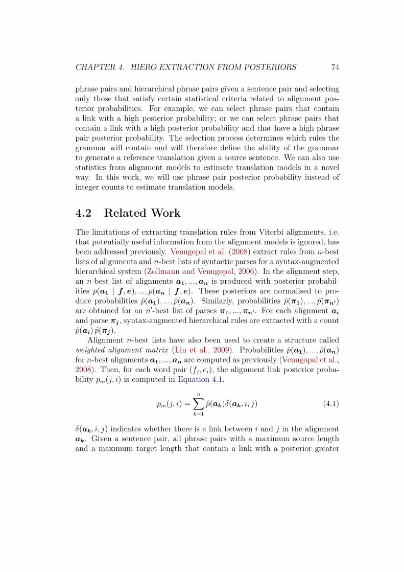
CHAPTER 4. HIERO EXTRACTION FROM POSTERIORS 74
phrase pairs and hierarchical phrase pairs given a sentence pair and selectingonly those that satisfy certain statistical criteria related to alignment pos-terior probabilities. For example, we can select phrase pairs that containa link with a high posterior probability; or we can select phrase pairs thatcontain a link with a high posterior probability and that have a high phrasepair posterior probability. The selection process determines which rules thegrammar will contain and will therefore define the ability of the grammarto generate a reference translation given a source sentence. We can also usestatistics from alignment models to estimate translation models in a novelway. In this work, we will use phrase pair posterior probability instead ofinteger counts to estimate translation models.
4.2 Related WorkThe limitations of extracting translation rules from Viterbi alignments, i.e.that potentially useful information from the alignment models is ignored, hasbeen addressed previously. Venugopal et al. (2008) extract rules from n-bestlists of alignments and n-best lists of syntactic parses for a syntax-augmentedhierarchical system (Zollmann and Venugopal, 2006). In the alignment step,an n-best list of alignments a1, ...,an is produced with posterior probabil-ities p(a1 | f , e), ..., p(an | f , e). These posteriors are normalised to pro-duce probabilities p(a1), ..., p(an). Similarly, probabilities p(π1), ..., p(πn′)are obtained for an n′-best list of parses π1, ...,πn′ . For each alignment ai
and parse πj , syntax-augmented hierarchical rules are extracted with a countp(ai) p(πj).
Alignment n-best lists have also been used to create a structure calledweighted alignment matrix (Liu et al., 2009). Probabilities p(a1), ..., p(an)for n-best alignments a1, ...,an are computed as previously (Venugopal et al.,2008). Then, for each word pair (fj, ei), the alignment link posterior proba-bility pm(j, i) is computed in Equation 4.1.
pm(j, i) =n∑
k=1
p(ak)δ(ak, i, j) (4.1)
δ(ak, i, j) indicates whether there is a link between i and j in the alignmentak. Given a sentence pair, all phrase pairs with a maximum source lengthand a maximum target length that contain a link with a posterior greater

CHAPTER 4. HIERO EXTRACTION FROM POSTERIORS 75
than zero are extracted. The fractional counts assigned to these phrase pairsare computed in terms of the link posteriors and then used to estimate thetranslation models by relative frequency. The fractional count computationapproximates the posterior probability of all alignments consistent with thephrase pair. Our method also uses link posterior probabilities to constrainthe extraction but the posteriors are computed exactly rather than approx-imated. In addition, posterior probabilities of consistent alignments is alsocomputed exactly. Finally, our method is also applied to hierarchical phrase-based translation.
Alignment posterior probabilities without approximation have also beenused. For a given test set, Deng and Byrne (2008) first extract phrase pairsin a standard manner. Then, source phrases in the test set that do nothave any corresponding target in the list of extracted phrase pairs are se-lected. For each of these source phrases, sentence pairs where the sourcephrase occurs are considered. For each such sentence pair, all target phrasesin the target sentence are assigned phrase pair posterior probabilities (seeSection 4.3.4) according to the source-to-target and target-to-source align-ment models, then ranked by the geometric average of the two probabilities.The top phrase pair is retained if its scores are above specific thresholds.Our definition of phrase pair posterior probabilities and the procedure tocompute them are directly inspired by the work we just described. However,we do not use the word-to-phrase HMM model but the simpler word-to-wordHMM model. In addition, our method is applied to hierarchical phrase-basedgrammars rather than simpler phrase-based grammars. Finally, our grammarextraction scheme does not consist in first extracting a standard grammarand then augmenting the grammar with additional rules: we modify the ex-traction procedure to directly extract a hierarchical grammar from alignmentlink posterior probabilities or phrase pair posterior probabilities.
Kumar et al. (2007) also use exact computation of alignment link pos-teriors in a different application setting. First, instead of using the Viterbicriterion for word alignment reminded in Equation 4.2,
a = argmaxa
p(f ,a | e) (4.2)
the maximum a posteriori criterion (Matusov et al., 2004), shown in Equa-tion 4.3, is used:
aj = argmaxi
p(aj = i | f , e) (4.3)

CHAPTER 4. HIERO EXTRACTION FROM POSTERIORS 76
Then, given a parallel corpus for three languages F , G, E, the link posteriorsfor the language pair (F , E) are computed in terms of the posteriors for thelanguage pair (F , G) and (G, E). G is called a bridge language. The moti-vation is that alignments for the F -G language pair and the G-E languagepair may inform alignment for F -E. Multiple bridge languages are used andproduce corresponding posterior matrices. The matrices are interpolated andalignments are extracted for each bridge language and for the interpolation.Translation gains are obtained in system combination.
We also note approaches to tighter coupling between hierarchical phrase-based grammars and alignments or even direct modelling of phrase alignment.Marcu and Wong (2002) introduce a joint phrase-based model that does notmake use of word alignments. In this generative model, a sentence pair isproduced by concatenating phrase pairs, or so-called concepts. The authorsconsider a simpler model with only joint phrase pair translation probabili-ties and a more complex model with translation and distortion probabilities.The parameter are trained with an approximate version of the expectation-maximisation algorithm (Dempster et al., 1977). Experiments demonstratetranslation improvements over IBM Model 4. Birch et al. (2006) constrainthis model in order to be able to apply it to larger parallel corpora. Whensearching for a set of phrase pairs to cover a training sentence pair, phrasepairs that are consistent with the intersection of Viterbi alignments (seeSection 2.3.2) are considered first; other phrase pairs are considered onlywhen the sentence pair cannot be covered entirely. Results close to standardphrase-based models are obtained.
DeNero and Klein (2008) prove that phrase alignment is an NP-hardproblem. Given a sentence pair (f , e), a bijective phrase alignment a isdefined as a bijective mapping between source phrases that form a partitionof f and target phrases that form a partition of e. A scoring function φis also defined that assigns a real-valued score to any phrase pair 〈sourcephrase, target phrase〉. The score of a bijective phrase alignment is simply theproduct of the scores of its phrase pairs. Given (f , e, φ), the phrase alignmentoptimisation problem is to find the best scoring alignment. DeNero and Klein(2008) show that this problem is NP-hard by showing that the correspondingdecision problem is NP-complete via reduction of the SAT problem. We givehere an indication of the size of the search space. The number of possiblesource partitions is 2|f |−1. Given a source partition with K+1 phrases, thereare (K + 1)! possible permutation of the source phrases and 2(
|e|−1K ) possible

CHAPTER 4. HIERO EXTRACTION FROM POSTERIORS 77
target partitions with K + 1 phrases. In conclusion, there is little hope tosolve the phrase alignment problem exactly.
Saers and Wu (2009) report an improvement on a phrase-based systemwhere word alignment has been trained with an inversion transduction gram-mar rather than IBM or HMM models. Phrase alignment is directly modelledwith an inversion transduction grammar. The phrase alignment search spaceis more restrictive than the space considered in DeNero and Klein (2008) andthe expectation maximisation algorithm can be carried out in O(n6) where nis the number of tokens in a sentence. Pauls et al. (2010) also use an inversiontransduction grammar to directly align phrases to nodes in a string-to-treemodel. Bayesian methods have also been developed to induce a grammardirectly from an unaligned parallel corpus (Blunsom et al., 2008b, 2009). Fi-nally, Cmejrek et al. (2009) extract rules directly from bilingual chart parsesof the parallel corpus without using word alignments. We take a differentapproach in that we aim to start with very strong alignment models and usethem to guide grammar extraction.
Finally, some work on smoothing, which could be complementary to theapproach taken in this thesis, has been conducted to address the shortcomingsof relative frequency estimation for translation models. Foster et al. (2006)conduct an extensive series of experiments that either replace the relativefrequency estimated phrase table by a smoothed phrase table or add thesmoothed phrase table as a feature and observe improvement in translationquality.
4.3 Rule ExtractionIn Section 4.2, we have reviewed approaches that “widen” the translationpipeline by using alignment n-best lists. We have also reviewed applicationsof exact computation of alignment posterior probabilities and attempts todirectly model phrase alignment. We will now describe our grammar extrac-tion methods, based on exact computation of alignment posterior probabili-ties under an alignment model. As in previous work (Hopkins et al., 2011),we first present a general approach that encompasses both standard methodsbased on rule extraction from Viterbi alignments as well as our methods. Forclarity of presentation, we first describe our methods in the simpler case ofphrase-based rule extraction, then extend them to hierarchical phrase-basedrule extraction.

CHAPTER 4. HIERO EXTRACTION FROM POSTERIORS 78
1: function ExtractRules(fJ1 , e
I1,a)
2: for 1 ≤ j1 ≤ j2 ≤ J do3: for 1 ≤ i1 ≤ i2 ≤ I do4: if SourceConstraints(f j2
j1)
∧ AlignConstraints(f j2j1, ei2i1 ,a)
∧ TargetConstraints(ei2i1) then5: Extract(X→〈f j2
j1,ei2i1〉, Count(f j2
j1, ei2i1))
6: end if7: end for8: end for9: end function
Figure 4.2: General procedure for phrase-based rule extraction: both tradi-tional rule extraction from Viterbi alignment and our method are instancesof this procedure.
4.3.1 General Framework for Rule Extraction
We first describe a general method for the extraction of phrase-based rules.An extension of this procedure for hierarchical rules is described in Sec-tion 4.3.5. The algorithm is described in Figure 4.2. Given a sentence pair(fJ
1 , eI1), for each source index pair (j1, j2) defining a source phrase f j2
j1(line
2), for each target index pair (i1, i2) defining a target phrase ei2i1 (line 3), ifsource constraints, target constraints and alignment constraints are satisfied(line 4), then the phrase pair (f j2
j1, ei2i1) is extracted with a certain count (line
5): the phrase pair is added to the list of phrase pairs used in translation, andthe count will be used subsequently to compute translation models by relativefrequency. The purpose of the constraints is to obtain a manageable numberof rules. If we did not impose constraints, we would extract I(I+1)J(J+1)
4(not
necessarily distinct) rules for the sentence pair (fJ1 , e
I1). During translation,
the decoder would need to apply more pruning, which would potentially leadto more search errors and a decrease in translation quality.
We will now refine this general procedure to make it more practical andcloser to a possible implementation. Let us call the source constraints CS, thealignment constraints CA and the target constraints CT . These are Booleanfunctions used to select phrase pairs. In practice, source constraints arechecked on the source phrases before looking at the target phrases. If source

CHAPTER 4. HIERO EXTRACTION FROM POSTERIORS 79
constraints are not met, then we need not consider target phrases for thatsource phrase. In addition, target phrases are only considered if they satisfyalignment constraints with the source phrase and, if they do, we rank themaccording to a certain ranking function R. Target constraints also dependon the ranking R, for example we can decide to keep only a certain num-ber of target phrases per source phrase. When a phrase pair is extracted,it is assigned a count which will be used to estimate the source-to-targetand target-to-source translation models. The counting function is called C.With this notation, we obtain the revised extraction procedure in Figure 4.3.We will now describe different rule extraction strategies in terms of the con-straints CS, CA, CT , the ranking function R and the counting function C.
4.3.2 Extraction from Viterbi Alignment Links
In this section, we describe the standard extraction procedure within theframework introduced in Section 4.3.1. Common practice takes a fixed set ofword alignment links L and extracts rules from this set. Alignment linksL are obtained from the alignment model a either by the Viterbi algo-rithm or by maximum a posteriori estimation (Matusov et al., 2004; Ku-mar et al., 2007) and possibly using symmetrisation heuristics to combinelinks obtained from source-to-target and target-to-source alignment models(see Section 2.3.2). We can restate this common approach in the frameworkproposed in Section 4.3.1 and in Figure 4.3 where constraints, ranking andcounting functions are defined as follows:
• source constraints CS(f j2j1):
j2 − j1 < smax (4.4)
where smax is a integer threshold defined experimentally. smax repre-sents the maximum length of a source phrase.
• alignment constraints CA(f j2j1, ei2i1 ,a):(
∀(j, i) ∈ L, j ∈ [j1, j2]⇔ i ∈ [i1, i2])∧(L∩[j1, j2]×[i1, i2] 6= ∅
)(4.5)
Alignment constraints have already been described in Section 2.5.3 asthe conditions required for phrase pair extraction. The first bracketedconstraint requires that there be no alignment link between a word

CHAPTER 4. HIERO EXTRACTION FROM POSTERIORS 80
1: function ExtractRules(fJ1 , e
I1,a)
2: for 1 ≤ j1 ≤ j2 ≤ J do3: if ¬CS(f j2
j1) then . Source constraints
4: continue5: end if6: T ← ∅ . Sorted target phrases7: for 1 ≤ i1 ≤ i2 ≤ I do8: if CA(f j2
j1, ei2i1 ,a) then . Alignment constraints
9: T ← T ∪ ei2i110: end if11: end for12: Sort(T,R) . Target phrases ranked according to R13: for ei2i1 ∈ T do14: if CT (ei2i1 , T ) then . Target constraints15: Extract(X→〈f j2
j1,ei2i1〉, C(f
j2j1, ei2i1))
16: end if17: end for18: end for19: end function
Figure 4.3: General procedure for phrase-based rule extraction. This versionis more practical and closer to a possible implementation than the algorithmin Figure 4.2. Source phrases are first considered. Only if source constraintsCS are satisfied, then target phrases are considered. Targets that satisfyalignment constraints CA with their source are ranked by R. Finally, phrasepairs where the target satisfies target constraints can be extracted with acertain count C. Note that the target constraints implicitly depend on theranking of the targets by R.

CHAPTER 4. HIERO EXTRACTION FROM POSTERIORS 81
inside the phrase pair and a word outside of it. The second bracketedconstraint requires that there be at least one alignment link in thephrase pair. Sometimes, an additional constraint specifies that theboundary words in the phrase pair should be aligned. In this work,this constraint is not present. A phrase pair that satisfies Equation 4.5is said to be consistent with the alignment (see Section 2.5.3).
• target constraints CT (ei2i1 , T ): no constraint is imposed in this work.Target constraints based on length may be imposed depending on theimplementation.
• ranking and counting functions:
R(f j2j1, ei2i1) = C(f
j2j1, ei2i1) = 1 (4.6)
The above constraints, ranking and counting functions define the standardapproach to grammar extraction. In the next sections, we depart from thisapproach and apply novel functions to rank and count target-side translationsaccording to their quality in the context of each parallel sentence, as definedby the word alignment models. We also depart from common practice in thatwe do not use a set of links as alignment constraints. We thus have bettercontrol over the number of extracted rules as well as the relative frequencyestimates of the source-to-target and target-to-source translation models.
4.3.3 Extraction from Posteriors Probabilities overAlignment Links
For presentation, we only consider source-to-target alignment models: therandom variable a that models the alignment process takes values in func-tions from source word positions to target word positions. However, it itpossible to apply our method with any directional alignment model. We willuse the link posterior probability p(aj = i | fJ
1 , eI1) to guide rule extraction.
This statistic expresses how likely it is that a word fj in source position jand a word ei in target position i are aligned given the sentence pair (fJ
1 , eI1).
The link posterior probability can be computed efficiently for Model 1, Model2 and HMM. In our experiments, we only use the HMM model to computelink posteriors but comparisons between link posteriors obtained from var-ious models may be interesting in the future. We will derive a closed form

CHAPTER 4. HIERO EXTRACTION FROM POSTERIORS 82
solution for these models to compute the link posterior probability. Applyingthe definition of conditional probability, we obtain the general form of thelink posterior probability in Equation 4.7.
p(aj0 = i0 | fJ1 , e
I1) =
p(aj0 = i0, fJ1 | eI1)
p(fJ1 | eI1)
(4.7)
Using Equation 4.7, we will now derive the link posterior probability pM1(aj0 =i0 | fJ
1 , eI1) for Model 1, pM2(aj0 = i0 | fJ
1 , eI1) for Model 2 and pHMM(aj0 =
i0 | fJ1 , e
I1) for the HMM model.
4.3.3.1 Link Posterior Probability for Model 1
Let us derive pM1(aj0 = i0 | fJ1 , e
I1), the link posterior probability under Model
1. We use the notation from (Brown et al., 1993), where t is the word-to-word translation table and ε is a constant. We compute the numerator fromEquation 4.7 by marginalising over all possible alignments and inverting sumand product signs to obtain Equation 4.8:
pM1(aj0 = i0, fJ1 | eI1)
=I∑
a1=0
...I∑
aj0−1=0
I∑aj0+1=0
...I∑
aJ=0
pM1(a1...aj0−1i0aj0+1...aJ , fJ1 | eI1)
=I∑
a1=0
...I∑
aj0−1=0
I∑aj0+1=0
...I∑
aJ=0
ε
(1 + I)Jt(fj0 | ei0)
J∏j=1j 6=j0
t(fj | eaj)
=ε
(1 + I)Jt(fj0 | ei0)
J∏j=1j 6=j0
I∑i=0
t(fj | ei) (4.8)
We compute the denominator from Equation 4.7 similarly (see Equation (15)in (Brown et al., 1993)) and obtain Equation 4.9:
pM1(fJ1 | eI1) =
ε
(1 + I)J
J∏j=1
I∑i=0
t(fj | ei) (4.9)
After simplification, we obtain Equation 4.10 from Equation 4.8 and Equa-tion 4.9:
pM1(aj0 = i0 | fJ1 , e
I1) =
t(fj0 |ei0)∑Ii=0 t(fj0 |ei)
(4.10)

CHAPTER 4. HIERO EXTRACTION FROM POSTERIORS 83
4.3.3.2 Link Posterior Probability for Model 2
We apply the same method to compute pM2(aj0 = i0 | fJ1 , e
I1), the link
posterior probability for Model 2. We also use notation from (Brown et al.,1993) but we replace the notation for the alignment probability a(i | j, J, I)by pa(i | j, J, I) for clarity. We compute the numerator from Equation 4.7 inEquation 4.11:
pM2(aj0 = i0, fJ1 | eI1)
=I∑
a1=0
...
I∑aj0−1=0
I∑aj0+1=0
...
I∑aJ=0
pM2(a1...aj0−1i0aj0+1...aJ , fJ1 | eI1)
=I∑
a1=0
...
I∑aj0−1=0
I∑aj0+1=0
...
I∑aJ=0
ε pa(i0 | j0, J, I) t(fj0 | ei0)
J∏j=1j 6=j0
pa(aj | j, J, I) t(fj | eaj)
= ε pa(i0 | j0, J, I) t(fj0 | ei0)J∏
j=1j 6=j0
I∑i=0
pa(i | j, J, I) t(fj | ei) (4.11)
We compute the denominator from Equation 4.7 similarly and obtain Equa-tion 4.12:
pM2(fJ1 | eI1) = ε
J∏j=1
I∑i=0
pa(i | j, J, I) t(fj | ei) (4.12)
After simplification, we obtain Equation 4.13 from Equation 4.11 and Equa-tion 4.12.
pM2(aj0 = i0 | fJ1 , e
I1) =
pa(i0 | j0, J, I) t(fj0 | ei0)∑Ii=0 pa(i | j0, J, I) t(fj0 | ei)
(4.13)
4.3.3.3 Link Posterior Probability for the HMM Model
We now derive pHMM(aj0 = i0|fJ1 , e
I1), the link posterior probability for the
HMM model (Vogel et al., 1996; Rabiner, 1989). These derivations are stan-dard once we realise that the observed sequence is the source sentence fJ
1 ,the hidden sequence is aJ1 and that in addition to standard presentations

CHAPTER 4. HIERO EXTRACTION FROM POSTERIORS 84
of HMM, all probabilities are conditioned on the target sentence eI1. Wecompute the numerator from Equation 4.7 in Equation 4.14:
pHMM(aj0 = i0, fJ1 | eI1) = pHMM(aj0 = i0, f
j01 , fJ
j0+1 | eI1)= pHMM(fJ
j0+1 | aj0 = i0, fj01 , eI1) pHMM(aj0 = i0, f
j01 | eI1)
= pHMM(fJj0+1 | aj0 = i0, e
I1) pHMM(aj0 = i0, f
j01 | eI1)
= βj0(i0) αj0(i0) (4.14)
where βj0(i0) and αj0(i0) are respectively the backward and forward HMMprobabilities defined in Equation 4.15:
βj(i) = pHMM(fJj+1 | aj = i, eI1)
αj(i) = pHMM(aj = i, f j1 | eI1)
(4.15)

CHAPTER 4. HIERO EXTRACTION FROM POSTERIORS 85
The forward and backward probabilities can be computed recursively asshown in Equation 4.16 and Equation 4.17:
αj(i) = pHMM(aj = i, f j1 | eI1)
=I∑
k=0
pHMM(aj = i, aj−1 = k, f j−11 , fj | eI1)
=I∑
k=0
pHMM(fj | aj = i, aj−1 = k, f j−11 , eI1) pHMM(aj = i, aj−1 = k, f j−1
1 | eI1)
=I∑
k=0
pHMM(fj | ei) pHMM(aj = i | aj−1 = k, f j−11 , eI1) pHMM(aj−1 = k, f j−1
1 | eI1)
=I∑
k=0
pHMM(fj | ei) pHMM(aj = i | aj−1 = k, I) αj−1(k) (4.16)
βj(i) = pHMM(fJj+1 | aj = i, eI1)
=I∑
k=0
pHMM(fJj+2, aj+1 = k, fj+1 | aj = i, eI1)
=I∑
k=0
pHMM(fJj+2 | aj+1 = k, fj+1, aj = i, eI1) pHMM(aj+1 = k, fj+1 | aj = i, eI1)
=I∑
k=0
pHMM(fJj+2 | aj+1 = k, eI1) pHMM(fj+1 | aj+1 = k, aj = i, eI1)
pHMM(aj+1 = k | aj = i, eI1)
=I∑
k=0
βj+1(k) pHMM(fj+1 | ek) pHMM(aj+1 = k | aj = i, I) (4.17)
The denominator from Equation 4.7 is computed in Equation 4.18:
pHMM(fJ1 | eI1) =
I∑k=0
pHMM(aJ = k, fJ1 | eI1)
=I∑
k=0
αJ(k) (4.18)
We will use the link posterior probabilities under the HMM model inorder to define constraints, ranking and counting functions.

CHAPTER 4. HIERO EXTRACTION FROM POSTERIORS 86
4.3.3.4 Constraints, Ranking and Counting Functions from HMMLink Posterior Probabilities
We use HMM link posterior probabilities computed in Section 4.3.3.3 in orderto define constraints, ranking and counting functions:
• source constraints CS(f j2j1):
j2 − j1 < smax (4.19)
This is the same constraint as defined for standard Viterbi extractionin Section 4.3.2.
• alignment constraints CA(f j2j1, ei2i1 ,a):
∃(j, i) ∈ [j1, j2]× [i1, i2], p(aj = i | fJ1 , e
I1) > λ (4.20)
∀(j, i) ∈ [1, J ]× [1, I] ∩ {(j, i) : p(aj = i | fJ1 , e
I1) > λ} (4.21)
j ∈ [j1, j2]⇔ i ∈ [i1, i2]
where λ is a threshold defined experimentally. Intuitively, λ is a highlink posterior probability. The first constraint (Equation 4.20) meansthat we require at least one link with a high posterior probability in thephrase pair considered. The second constraint (Equation 4.21) meansthat there should be no link with a high posterior probability thatbe inconsistent with the phrase pair. Note that these constraints areidentical to the Viterbi alignment constraints defined in Section 4.3.2if we choose L to be the set of all links with high posterior defined inEquation 4.22:
L = {(j, i) ∈ [1, J ]× [1, I] : p(aj = i | fJ1 , e
I1) > λ} (4.22)
Also note that the second constraint does not consider links to the nullword (see Section 2.3) relevant. This is because we do not need toinclude the null word in a translation rule.
• target constraints CT (ei2i1 , T ): we pick the first k translation candidatesaccording to the ranking function R.
• ranking function:
R(f j2j1, ei2i1) =
j2∏j=j1
i2∑i=i1
p(aj = i | fJ1 , e
I1)
i2 − i1 + 1(4.23)

CHAPTER 4. HIERO EXTRACTION FROM POSTERIORS 87
This ranking function is very similar to the score used for lexical fea-tures described in Section 2.6.5. Here, we use link posteriors insteadof Model 1 translation probabilities. This function favours short targetphrases, therefore we do not use it as a counting function. Preliminaryexperiments found that this function is not appropriate for countingrules and that it gives poor results. We therefore use the same count-ing function as in standard practice described in Section 4.3.2.
• counting function:C(f j2
j1, ei2i1) = 1 (4.24)
We have described rule extraction from alignment link posterior prob-abilities. Next, we will describe rule extraction from alignment posteriorprobabilities over phrase pairs. This method will use the same source con-straints, alignment constraints and target constraints but different rankingand counting functions.
4.3.4 Extraction from Posteriors over Phrase Pairs
In the previous section, we defined and gave closed form solutions to align-ment link posterior probabilities for Model 1, Model 2 and the HMM model.We can also define alignment posterior probabilities over phrase pairs. Letus consider the phrase pair 〈f j2
j1, ei2i1〉 in the sentence pair (fJ
1 , eI1). In Equa-
tion 4.25, we define A(j1, j2; i1, i2), the set of alignments that have no linksbetween inside the phrase pair and outside the phrase pair:
A(j1, j2; i1, i2) = {aJ1 : aj ∈ [i1, i2]⇔ j ∈ [j1, j2]} (4.25)
Alignments in A(j1, j2; i1, i2) satisfy the consistency constraint defined inEquation 4.5 but do not require a link in [j1, j2] × [i1, i2]. The posteriorprobability of these alignments given the sentence pair is defined in Equa-tion 4.26:
p(A(j1, j2; i1, i2) | eI1, fJ1 ) =
p(fJ1 , A(j1, j2; i1, i2) | eI1)
p(fJ1 | eI1)
=
∑aJ1∈A(j1,j2;i1,i2)
p(fJ1 , a
J1 | eI1)∑
aJ1p(fJ
1 , aJ1 | eI1)
(4.26)
We call this quantity the phrase pair posterior probability. We will now deriveformula for the phrase pair posterior probability in the case of Model 1, Model
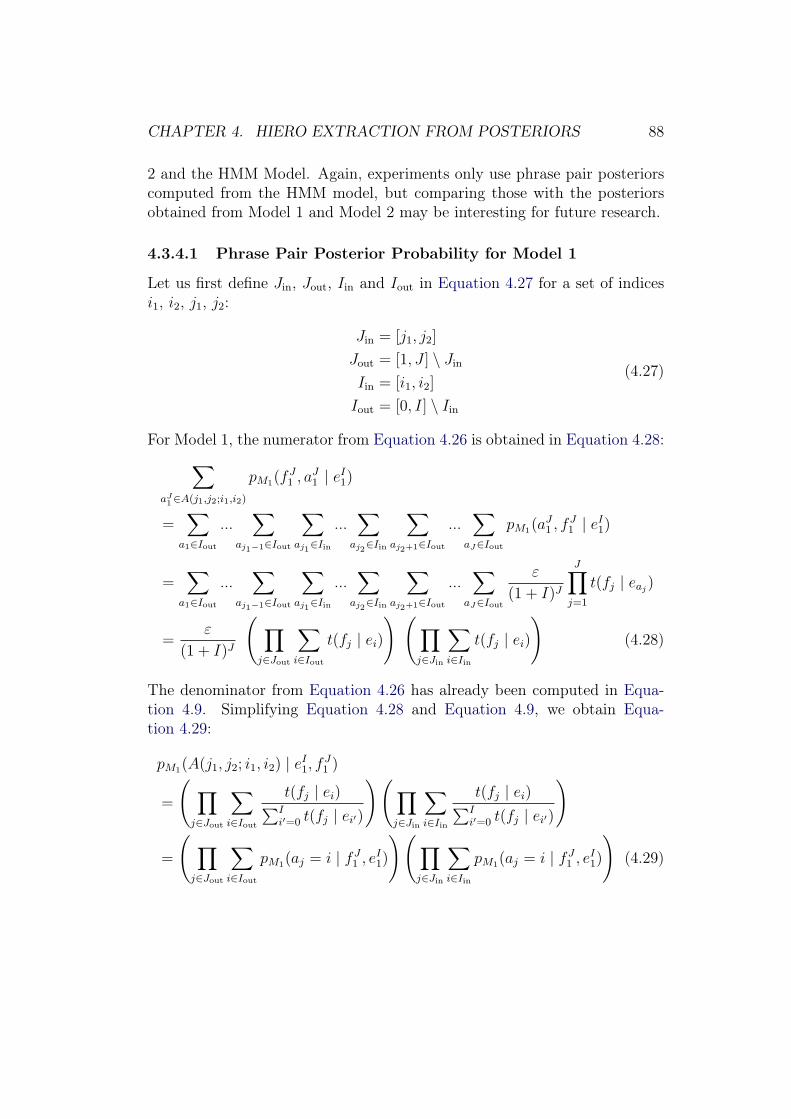
CHAPTER 4. HIERO EXTRACTION FROM POSTERIORS 88
2 and the HMM Model. Again, experiments only use phrase pair posteriorscomputed from the HMM model, but comparing those with the posteriorsobtained from Model 1 and Model 2 may be interesting for future research.
4.3.4.1 Phrase Pair Posterior Probability for Model 1
Let us first define Jin, Jout, Iin and Iout in Equation 4.27 for a set of indicesi1, i2, j1, j2:
Jin = [j1, j2]
Jout = [1, J ] \ Jin
Iin = [i1, i2]
Iout = [0, I] \ Iin
(4.27)
For Model 1, the numerator from Equation 4.26 is obtained in Equation 4.28:∑aJ1∈A(j1,j2;i1,i2)
pM1(fJ1 , a
J1 | eI1)
=∑
a1∈Iout
...∑
aj1−1∈Iout
∑aj1∈Iin
...∑
aj2∈Iin
∑aj2+1∈Iout
...∑
aJ∈Iout
pM1(aJ1 , f
J1 | eI1)
=∑
a1∈Iout
...∑
aj1−1∈Iout
∑aj1∈Iin
...∑
aj2∈Iin
∑aj2+1∈Iout
...∑
aJ∈Iout
ε
(1 + I)J
J∏j=1
t(fj | eaj)
=ε
(1 + I)J
( ∏j∈Jout
∑i∈Iout
t(fj | ei)
) (∏j∈Jin
∑i∈Iin
t(fj | ei)
)(4.28)
The denominator from Equation 4.26 has already been computed in Equa-tion 4.9. Simplifying Equation 4.28 and Equation 4.9, we obtain Equa-tion 4.29:
pM1(A(j1, j2; i1, i2) | eI1, fJ1 )
=
( ∏j∈Jout
∑i∈Iout
t(fj | ei)∑Ii′=0 t(fj | ei′)
)(∏j∈Jin
∑i∈Iin
t(fj | ei)∑Ii′=0 t(fj | ei′)
)
=
( ∏j∈Jout
∑i∈Iout
pM1(aj = i | fJ1 , e
I1)
)(∏j∈Jin
∑i∈Iin
pM1(aj = i | fJ1 , e
I1)
)(4.29)

CHAPTER 4. HIERO EXTRACTION FROM POSTERIORS 89
4.3.4.2 Phrase Pair Posterior Probability for Model 2
To avoid repetition, we skip the derivation which is analogous to the deriva-tion for Model 1. We obtain the phrase pair posterior in Equation 4.30:
pM2(A(j1, j2; i1, i2) | eI1, fJ1 )
=
( ∏j∈Jout
∑i∈Iout
pM2(aj = i | fJ1 , e
I1)
)(∏j∈Jin
∑i∈Iin
pM2(aj = i | fJ1 , e
I1)
)(4.30)
4.3.4.3 Phrase Pair Posterior Probability for HMM
Let us now compute the phrase pair posterior probability for the HMMmodel. The denominator from Equation 4.26 can be computed using theforward algorithm while the numerator can be computed using a modifiedforward algorithm (Deng, 2005). Let us define αj(i), the modified forwardprobability in Equation 4.31:
αj(i) = pHMM(A(j1, j2; i1, i2), fj1 , aj = i | eI1) (4.31)
The numerator from Equation 4.26 can be computed in Equation 4.32:
p(A(j1, j2; i1, i2), fJ1 | eI1) =
I∑i=0
αJ(i) (4.32)
The denominator from Equation 4.26 can be computed using the regularforward probability in Equation 4.33:
p(fJ1 | eI1) =
I∑i=0
αJ(i) (4.33)
Like the regular forward probability, the modified forward probability canalso be computed recursively. We can also write the modified forward prob-ability as in Equation 4.34:
αj(i) = pHMM(A(j1, j2; i1, i2), fj1 , aj = i | eI1)
=∑
aj1∈A(j1,j2;i1,i2)
pHMM(aj−11 , f j
1 , aj = i | eI1)
=∑
aj1∈A(j1,j2;i1,i2)aj=i
pHMM(aj−11 , f j
1 , aj = i | eI1)(4.34)

CHAPTER 4. HIERO EXTRACTION FROM POSTERIORS 90
The computation of αj(i) is by a constrained forward algorithm where theconstraint is given in Equation 4.35. This is because an alignment in A(j1, j2; i1, i2)cannot have a link from inside the phrase pair to outside the phrase pair (seeEquation 4.25):
∀(j, i) ∈ Jout × Iin ∪ Jin × Iout, αj(i) = 0 (4.35)
For a link (j, i) ∈ Jout×Iout∪Jin×Iin that satisfies the constraint from Equa-tion 4.35, we can derive the modified forward probability in Equation 4.36:
αj(i) = pHMM(A(j1, j2; i1, i2), fj1 , aj = i | eI1)
=∑
aj−11 ∈A(j1,j2;i1,i2)
pHMM(fj, fj−11 , aj = i, aj−1
1 | eI1)
=∑
aj−11 ∈A(j1,j2;i1,i2)
pHMM(fj | f j−11 , aj = i, aj−1
1 , eI1)×
pHMM(aj = i | f j−11 , aj−1
1 , eI1)×pHMM(f j−1
1 , aj−11 | eI1)
= pHMM(fj | ei)∑
aj−11 ∈A(j1,j2;i1,i2)
pHMM(aj = i | aj−1, I) pHMM(f j−11 , aj−1
1 | eI1)
= pHMM(fj | ei)I∑
k=0
∑aj−11 ∈A(j1,j2;i1,i2)
aj−1=k
pHMM(aj = i | aj−1 = k, I)
pHMM(f j−11 , aj−1 = k, aj−2
1 | eI1)
= pHMM(fj | ei)I∑
k=0
pHMM(aj = i | aj−1 = k, I)∑aj−11 ∈A(j1,j2;i1,i2)
aj−1=k
pHMM(f j−11 , aj−1 = k, aj−2
1 | eI1)
= pHMM(fj | ei)I∑
k=0
pHMM(aj = i | aj−1 = k, I) αj−1(k) (4.36)
We will use the phrase pair posterior probabilities under the HMM model inorder to define ranking and counting functions.

CHAPTER 4. HIERO EXTRACTION FROM POSTERIORS 91
4.3.4.4 Constraints, Ranking and Counting Functions from HMMLink and Phrase Posterior Probabilities
In order to keep the size of the rule set manageable, we use the same sourceconstraints, alignment constraints and target constraints as for link posteriorextraction defined in Section 4.3.3. We use the phrase pair posterior proba-bilities under the HMM model both for ranking and scoring extracted rules.This approach assigns a fractional count to each extracted rule, which al-lows finer estimation of the source-to-target and target-to-source translationmodels. The ranking and counting functions are defined in Equation 4.37:
R(f j2j1, ei2i1) = C(f
j2j1, ei2i1) = pHMM(A(j1, j2; i1, i2) | f j
1 , eJ1 ) (4.37)
Under the framework described in Section 4.3.1, we have described stan-dard rule extraction from Viterbi alignments and two novel approaches torule extraction based on link posterior probabilities and phrase pair pos-terior probabilities. In order to expose concepts with more clarity, we haverestricted the presentation to the extraction of phrase based rules as opposedto hierarchical rules. We will now show how to generalise the techniques pre-sented so far to the extraction of hierarchical rules.
4.3.5 Hierarchical Rule Extraction
In this section, we extend the techniques presented so far to hierarchical ruleextraction. In order to avoid repetition, we describe these techniques forthe rule pattern 〈wXw,wXw〉 only (see Section 2.6.2.4 for the definition ofpatterns). We first rewrite the algorithm in Figure 4.3 into the algorithm inFigure 4.4 for this pattern. We will now describe constraints, counting andranking functions for standard Viterbi extraction and for extraction fromalignment posteriors.
4.3.5.1 Hierarchical Rule Extraction from Viterbi Alignment Links
We now describe the constraints, ranking and counting functions for hierar-chical rule extraction from Viterbi alignments:

CHAPTER 4. HIERO EXTRACTION FROM POSTERIORS 92
1: function ExtractRules(fJ1 , e
I1,a)
2: for 1 ≤ j1 ≤ j2 < j3 ≤ j4 ≤ J do3: if ¬CS(f j2
j1Xf j4
j3) then . Source constraints
4: continue5: end if6: T ← ∅ . Sorted hierarchical target phrases7: for 1 ≤ i1 ≤ i2 < i3 ≤ i4 ≤ I do8: if CA(f j2
j1Xf j4
j3, ei2i1Xei4i3 ,a) then . Alignment constraints
9: T ← T ∪ ei2i1Xei4i310: end if11: end for12: Sort(T,R) . Hierarchical target phrases ranked according to R13: for ei2i1Xei4i3 ∈ T do14: if CT (ei2i1Xei4i3 , T ) then . Target constraints15: Extract(X→〈f j2
j1Xf j4
j3,ei2i1Xei4i3〉, C(f
j2j1Xf j4
j3, ei2i1Xei4i3))
16: end if17: end for18: end for19: end function
Figure 4.4: General procedure for hierarchical phrase-based rule extraction.The procedure is presented for the pattern 〈wXw,wXw〉 only. This algo-rithm is analogous to the algorithm used to extract phrase-based rules andpresented in Figure 4.3.

CHAPTER 4. HIERO EXTRACTION FROM POSTERIORS 93
• source constraints CS(f j2j1Xf j4
j3):
(j2 − j1 + 1) + 1 + (j4 − j3 + 1) ≤ smax elements
j2 − j1 < smax terminals
j4 − j3 < smax terminals
span(X) ≤ smax NT
(4.38)
We remind definitions introduced in Section 3.5.2 for the thresholds inEquation 4.38. smax elements is the maximum number of terminals andnonterminals in the source. smax terminals is the maximum number ofconsecutive terminals in the source. smax NT is the maximum span fora nonterminal, i.e. the maximum number of terminals covered by anonterminal. These thresholds are defined experimentally.
• alignment constraints CA(f j2j1Xf j4
j3, ei2i1Xei4i3 ,a):
∀(j, i) ∈ L, j ∈ [j1, j4]⇔ i ∈ [i1, i4]
L ∩ [j1, j4]× [i1, i4] 6= ∅∀(j, i) ∈ L, j ∈ (j2, j3)⇔ i ∈ (i2, i3)
L ∩ {j2 + 1} × (i2, i3) 6= ∅L ∩ {j3 − 1} × (i2, i3) 6= ∅L ∩ (j2, j3)× {i2 + 1} 6= ∅L ∩ (j2, j3)× {i3 − 1} 6= ∅
(4.39)
The first two constraints require that that the phrase pair (f j4j1, ei4i1) be
consistent with the links L. The third constraint requires that therebe no link from inside the phrase pair (f j3−1
j2+1 , ei3−1i2+1), which corresponds
to the nonterminal X, to outside the phrase pair. The last four con-straints mean that the boundary words fj2+1, fj3−1, ei2+1, ei3−1 are notunaligned.
• target constraints CT (ei2i1Xei4i3 , T ): no constraint. Again, other imple-mentations may impose for example length-based constraints on thetarget.
• ranking and counting functions:
R(f j2j1Xf j4
j3, ei2i1Xei4i3) = C(f
j2j1Xf j4
j3, ei2i1Xei4i3) = 1 (4.40)

CHAPTER 4. HIERO EXTRACTION FROM POSTERIORS 94
4.3.5.2 Hierarchical Rule Extraction from Link Posterior Proba-bilities
We now describe the constraints, ranking and counting functions for the linkposterior extraction of hierarchical rules:
• source constraints CS(f j2j1Xf j4
j3):
j2 − j1 < shier max
j4 − j3 < shier max
j3 − j2 < smax NT
(4.41)
shier max is the maximum length for consecutive terminals in the source.smax NT is the maximum number of terminals covered by a nonterminal.These thresholds are defined experimentally.
• For alignment constraints, let us first define Jin, Jout, Iin and Iout inEquation 4.42 for a set of indices i1, i2, i3, i4, j1, j2, j3, j4:
Jin = [j1, j2] ∪ [j3, j4]
Jout = [1, J ] \ Jin
Iin = [i1, i2] ∪ [i3, i4]
Iout = [0, I] \ Iin
(4.42)
Alignment constraints CA(f j2j1Xf j4
j3, ei2i1Xei4i3 ,a) are defined in Equation 4.43.
∃(j, i) ∈ (j2, j3)× (i2, i3), p(aj = i | fJ1 , e
I1) > λ
∃(j, i) ∈ [j1, j2]× Iin, p(aj = i | fJ1 , e
I1) > λ
∃(j, i) ∈ [j3, j4]× Iin, p(aj = i | fJ1 , e
I1) > λ
∃(j, i) ∈ Jin × [i1, i2], p(aj = i | fJ1 , e
I1) > λ
∃(j, i) ∈ Jin × [i3, i4], p(aj = i | fJ1 , e
I1) > λ
∀(j, i) ∈ [1, J ]× [1, I] ∩ {(j, i) : p(aj = i | fJ1 , e
I1) > λ}
j ∈ (j2, j3)⇔ i ∈ (i2, i3)
j ∈ Jin ⇔ i ∈ Iin
(4.43)
• target constraints CT (ei2i1Xei4i3 , T ):
i2 − i1 < thier max
i4 − i3 < thier max(4.44)
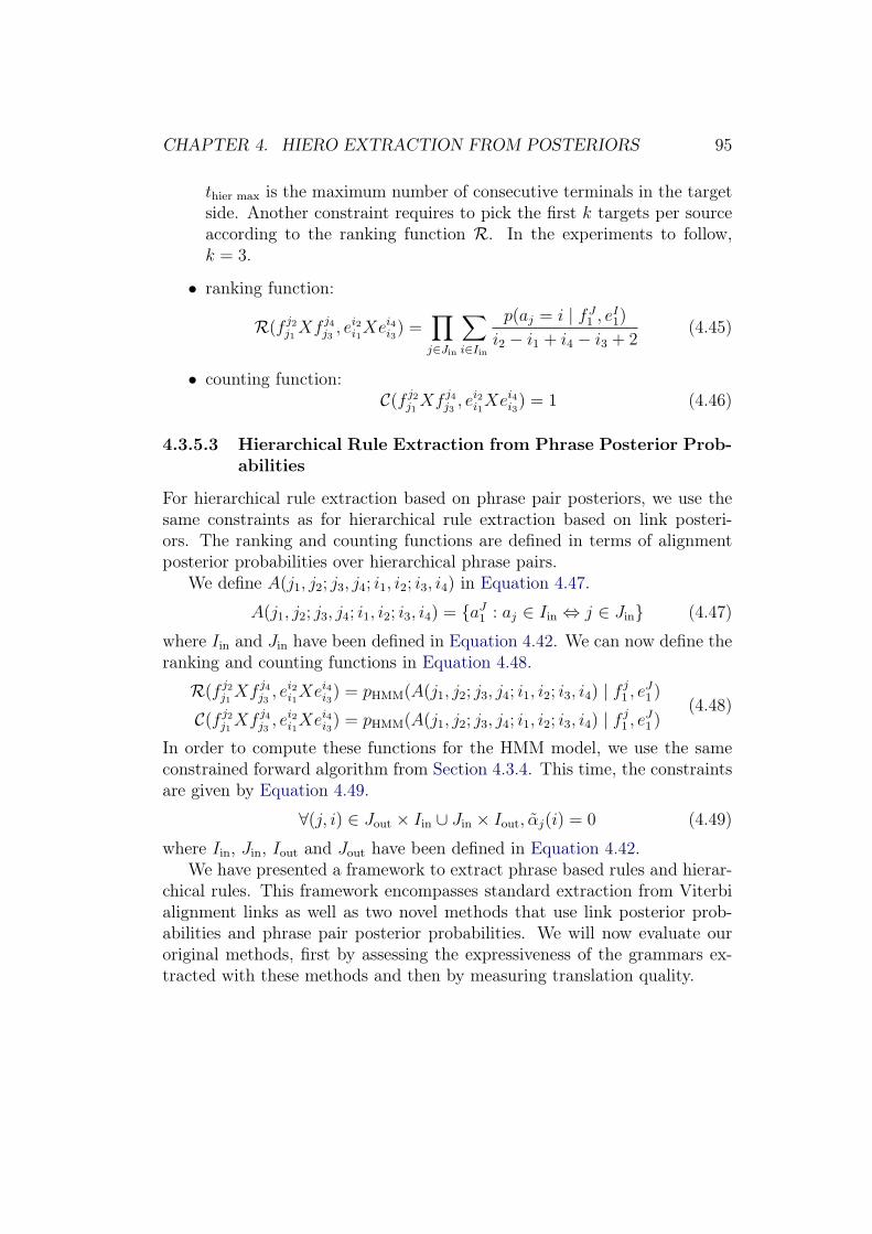
CHAPTER 4. HIERO EXTRACTION FROM POSTERIORS 95
thier max is the maximum number of consecutive terminals in the targetside. Another constraint requires to pick the first k targets per sourceaccording to the ranking function R. In the experiments to follow,k = 3.
• ranking function:
R(f j2j1Xf j4
j3, ei2i1Xei4i3) =
∏j∈Jin
∑i∈Iin
p(aj = i | fJ1 , e
I1)
i2 − i1 + i4 − i3 + 2(4.45)
• counting function:C(f j2
j1Xf j4
j3, ei2i1Xei4i3) = 1 (4.46)
4.3.5.3 Hierarchical Rule Extraction from Phrase Posterior Prob-abilities
For hierarchical rule extraction based on phrase pair posteriors, we use thesame constraints as for hierarchical rule extraction based on link posteri-ors. The ranking and counting functions are defined in terms of alignmentposterior probabilities over hierarchical phrase pairs.
We define A(j1, j2; j3, j4; i1, i2; i3, i4) in Equation 4.47.
A(j1, j2; j3, j4; i1, i2; i3, i4) = {aJ1 : aj ∈ Iin ⇔ j ∈ Jin} (4.47)
where Iin and Jin have been defined in Equation 4.42. We can now define theranking and counting functions in Equation 4.48.
R(f j2j1Xf j4
j3, ei2i1Xei4i3) = pHMM(A(j1, j2; j3, j4; i1, i2; i3, i4) | f j
1 , eJ1 )
C(f j2j1Xf j4
j3, ei2i1Xei4i3) = pHMM(A(j1, j2; j3, j4; i1, i2; i3, i4) | f j
1 , eJ1 )
(4.48)
In order to compute these functions for the HMM model, we use the sameconstrained forward algorithm from Section 4.3.4. This time, the constraintsare given by Equation 4.49.
∀(j, i) ∈ Jout × Iin ∪ Jin × Iout, αj(i) = 0 (4.49)
where Iin, Jin, Iout and Jout have been defined in Equation 4.42.We have presented a framework to extract phrase based rules and hierar-
chical rules. This framework encompasses standard extraction from Viterbialignment links as well as two novel methods that use link posterior prob-abilities and phrase pair posterior probabilities. We will now evaluate ouroriginal methods, first by assessing the expressiveness of the grammars ex-tracted with these methods and then by measuring translation quality.

CHAPTER 4. HIERO EXTRACTION FROM POSTERIORS 96
G0 G1 G2 G3 G4S→〈X,X〉 X→〈w X,X w〉 X→〈w X,X w〉 X→〈w X,X w〉 X→〈w X,X w〉
S→〈S X,S X〉 X→〈X w,w X〉 X→〈X w,w X〉 X→〈X w,w X〉 X→〈X w,w X〉X→〈w,w〉 X→〈w X,w X〉 X→〈w X,w X〉 X→〈X1wX2,wX2X1〉
X→〈w X w,w X w〉 X→〈X1wX2,X2X1w〉
Table 4.1: Hierarchical phrase-based grammars containing different typesof rules. The grammar expressiveness is greater as more types of rules areincluded. In addition to the rules shown in the respective columns, G1, G2,G3 and G4 also contain the rules of G0.
4.4 ExperimentsIn this section, we carry out experiments in order to demonstrate the ef-fectiveness of our original grammar extraction method. We will assess thequality of the grammars extracted in terms of how expressive these grammarsare, and in terms of translation quality. In Section 4.4.1, we define the pat-terns to be included in the grammars used for experiments. In Section 4.4.2,we describe our experimental setup. In Section 4.4.3 and Section 4.4.4, wereport results for grammar expressiveness and translation quality. In Sec-tion 4.4.5, we compare our two original methods: link posterior extractionvs. phrase pair posterior extraction. Finally, in Section 4.4.6, we explorevarious methods to exploit information from source-to-target and target-to-source alignment models.
4.4.1 Experimental Setup: Grammar Pattern Defini-tion
In this section we define the hierarchical phrase-based grammars we use fortranslation experiments. Each grammar is defined by the patterns it contains(see Section 2.6.2.4). We first start with a basic grammar G0 defined in theleft-most column of Table 4.1. G0 is a monotonic phrase-based translationgrammar. It includes all phrase-based rules, represented by the rule patternX → 〈w,w〉, and the two glue rules that allow concatenation.
Our approach is to extend this grammar by successively incorporatingsets of hierarchical rules, or patterns. The goal is to obtain a grammar withfew rule patterns but capable of generating a large collection of translationcandidates for a given input sentence.
Patterns were added to the base grammar G0 according to their frequency
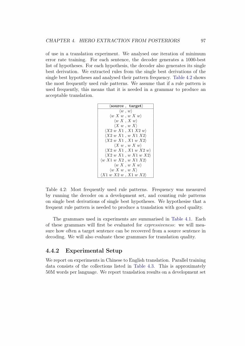
CHAPTER 4. HIERO EXTRACTION FROM POSTERIORS 97
of use in a translation experiment. We analysed one iteration of minimumerror rate training. For each sentence, the decoder generates a 1000-bestlist of hypotheses. For each hypothesis, the decoder also generates its singlebest derivation. We extracted rules from the single best derivations of thesingle best hypotheses and analysed their pattern frequency. Table 4.2 showsthe most frequently used rule patterns. We assume that if a rule pattern isused frequently, this means that it is needed in a grammar to produce anacceptable translation.
〈source , target〉〈w , w〉
〈w X w , w X w〉〈w X , X w〉〈X w , w X〉
〈X2 w X1 , X1 X2 w〉〈X2 w X1 , w X1 X2〉〈X2 w X1 , X1 w X2〉
〈X w , w X w〉〈X2 w X1 , X1 w X2 w〉〈X2 w X1 , w X1 w X2〉
〈w X1 w X2 , w X1 X2〉〈w X , w X w〉
〈w X w , w X〉〈X1 w X2 w , X1 w X2〉
Table 4.2: Most frequently used rule patterns. Frequency was measuredby running the decoder on a development set, and counting rule patternson single best derivations of single best hypotheses. We hypothesise that afrequent rule pattern is needed to produce a translation with good quality.
The grammars used in experiments are summarised in Table 4.1. Eachof these grammars will first be evaluated for expressiveness: we will mea-sure how often a target sentence can be recovered from a source sentence indecoding. We will also evaluate these grammars for translation quality.
4.4.2 Experimental Setup
We report on experiments in Chinese to English translation. Parallel trainingdata consists of the collections listed in Table 4.3. This is approximately50M words per language. We report translation results on a development set

CHAPTER 4. HIERO EXTRACTION FROM POSTERIORS 98
ADSO_v5 LDC2006E26 LDC2007E87LDC2002L27 LDC2006E34 LDC2008E40LDC2003E07 LDC2006E85 LDC2008E56LDC2003E14 LDC2006E92 LDC2008G05LDC2005E83 LDC2006G05 LDC2009E16LDC2005T06 LDC2007E06 LDC2009G01LDC2005T10 LDC2007E101 proj_syndicateLDC2005T34 LDC2007E103 UMD_NewsExplorerLDC2006E24 LDC2007E46 Wikipedia
Table 4.3: List of collections used as parallel training data for translationexperiments.
tune-nw and a test set test-nw1. These contain translations produced by theGALE program and portions of the newswire sections of NIST MT02 throughMT06.1 They contain 1755 sentences and 1671 sentences respectively. Resultsare also reported on a smaller held-out test set test-nw2, containing 60% ofthe NIST newswire portion of MT06, that is, 369 sentences. In Section 4.4.5,the entire newswire portion of MT06 is used and the test set is named test-nw3.
The parallel texts for both language pairs are aligned using MTTK (Dengand Byrne, 2005, 2008). For decoding, we use HiFST (see Section 2.9).The language model is a 4-gram language model estimated over the Englishside of the parallel text and the AFP and Xinhua portions of the EnglishGigaword Fourth Edition (LDC2009T13) for the first pass translation, in-terpolated with a zero-cutoff Stupid Backoff 5-gram (see Section 2.7.4 andSection 3.2) estimated using 10.5B words of English newswire text for 5-gramlanguage model rescoring. In tuning the systems, standard minimum errorrate training iterative parameter estimation under BLEU is performed onthe development set.
Rules with a source-to-target probability less than 0.01 are discarded. Inaddition, rules that did not occur more than nobs times are discarded. ForViterbi extraction, nobs = 1. For link posterior extraction, nobs = 2 andfor phrase pair posterior extraction, nobs = 0.2. These thresholds offer weredefined experimentally and provide competitive performance for the various
1 http://www.itl.nist.gov/iad/mig/tests/mt
CHAPTER 4. HIERO EXTRACTION FROM POSTERIORS 99
conditions without giving unreasonably slow decoding times. The thresholdsintroduced in previous sections are defined as follows:
• smax is set to 9 for Viterbi extraction and to 5 for posterior extraction.A preliminary experiment showed that for posterior extraction, settingsmax to 9 did not provide any improvements and slowed down decodingtimes.
• smax elements is set to 5.
• smax terminals is set to 5.
• smax NT is set to 10.
• λ is set to 0.5.
• shier max and thier max are set to 3.
The thresholds relating to Viterbi extraction (smax, smax elements, smax terminals,smax NT) are standard in our translation systems. λ, shier max and thier max werechosen experimentally and provide competitive performance without slowingdown decoding unreasonably.
4.4.3 Grammar Coverage
We first evaluate the grammars defined in Section 4.4.1 for expressiveness.We measure the ability of different grammars to produce a reference transla-tion given an input sentence. Rules are extracted from the sentence pair wewant to align and we run the decoder in alignment mode (de Gispert et al.,2010a), which is equivalent to replacing the language model by an accep-tor for the reference translation. We compare the percentage of referencesthat can be successfully produced by grammars G0, G1, G2 and G3
2 for thefollowing extraction methods:
• Viterbi (V): this is the standard extraction method based on a setof alignment links. We distinguish four cases, depending on the modelused to obtain the set of links: source-to-target (V-st), target-to-source(V-ts), and two common symmetrisation strategies: union (V-union)and grow-diag-final (V-gdf) (see Section 2.3.2).
2 We did not include G4 in coverage analysis

CHAPTER 4. HIERO EXTRACTION FROM POSTERIORS 100
30
40
50
60
70
80
V-stV-ts
V-union
V-gdf
V-merge
WP-st
WP-ts
WP-m
erge
G0G1G2G3
Figure 4.5: Percentage of parallel sentences successfully aligned for variousextraction methods and grammars.
• Word Link Posteriors (WP): the extraction method is based on linkposteriors described in Section 4.3.3. These rules can be obtained eitherfrom the posteriors of the source-to-target (WP-st) or the target-to-source (WP-ts) alignment models. We apply the constraints describedin Section 4.3.3. We do not report alignment percentages when usingphrase pair posteriors as they are roughly identical to the WP case.
• Finally, in both cases, we also report results when merging the extractedrules in both directions into a single rule set (V-merge and WP-merge).
Figure 4.5 shows the results obtained for a random selection of 10,000 parallelcorpus sentences. As expected, we can see that for any extraction method,the percentage of aligned sentences increases when switching from G0 toG1, G2 and G3. Posterior-based extraction is shown to outperform standardmethods based on a Viterbi set of alignment links for nearly all grammars.The highest alignment percentages are obtained when merging rules obtainedunder models trained in each direction (WP-merge), approximately reach-ing 80% for grammar G3.

CHAPTER 4. HIERO EXTRACTION FROM POSTERIORS 101
The maximum rule span (smax span defined in Section 3.5.2) in alignmentwas allowed to be 15 words, so as to be similar to translation, where themaximum rule span is 10 words. Relaxing this in alignment to 30 wordsyields approximately 90% coverage for WP-merge under G3.
We note that if source constraints, alignment constraints and target con-straints were not applied, then alignment percentages would be 100% evenfor G0, but the extracted grammar would include many noisy rules with poorgeneralisation power, for example entire sentence pairs.
4.4.4 Translation Results
In this section we investigate the translation performance of each hierarchicalgrammar, as defined by rules obtained from three rule extraction methods:
• Viterbi union (V-union): standard rule extraction from the unionof the source-to-target and target-to-source alignment link sets.
• Word Posteriors (WP-st): extraction based on word posteriors asdescribed in Section 4.3.3. The posteriors are provided by the source-to-target alignment model.
• Phrase Posteriors (PP-st): extraction based on alignment poste-riors over phrase pairs, as described in Section 4.3.4, with fractionalcounts equal to the phrase pair posterior probability under the source-to-target alignment model.
Table 4.4 reports the translation results. It also shows the following decodingstatistics as measured on the tune-nw set: decoding time in seconds per inputword, and number of instances of search pruning per input word. Preliminaryexperimental work was conducted on grammars G1 and G2. Because of slowdecoding times, G4 was not included in this set of experiments; instead, gram-mar G4 was used to contrast the WP and PP methods in Section 4.4.5. Asa contrast, we extract rules according to the heuristics introduced by Chiang(2007) and apply the filters described by Iglesias et al. (2009a) to generate astandard hierarchical phrase-based grammar GH described in Section 2.6.2.4.This uses rules with up to two nonadjacent nonterminals, but excludes iden-tical rule types such as X→〈w X,w X〉 or X→〈w X1 w X2,w X1 w X2〉,which were reported to cause computational difficulties without a clear im-provement in translation (Iglesias et al., 2009a).

CHAPTER 4. HIERO EXTRACTION FROM POSTERIORS 102
Grammar Extraction # Rules tune-nw test-nw1 test-nw2time prune BLEU BLEU BLEU
GH V-union 979k 3.7 0.3 35.1 35.6 37.6V-union 614k 0.4 0.0 33.6 34.6 36.4
G1 WP-st 920k 0.9 0.0 34.3 34.8 37.5PP-st 894k 1.4 0.0 34.4 35.1 37.7V-union 735k 1.0 0.0 34.5 35.4 37.2
G2 WP-st 1132k 5.8 0.5 35.1 36.0 37.7PP-st 1238k 7.8 0.7 35.5 36.4 38.2V-union 967k 1.2 0.0 34.9 35.3 37.0
G3 WP-st 2681k 8.3 1.1 35.1 36.2 37.9PP-st 5002k 10.7 2.6 35.5 36.4 38.5
Table 4.4: Chinese to English translation results with alternative grammarsand extraction methods (lower-cased BLEU shown). The number of rulesand time (secs/word) and prune (times/word) measurements are done ontune-nw set.
Condition tune-nw test-nw1GH/V-union 34.60/34.56/0.02/0.41 34.89/34.73/0.03/0.52G2/PP-st 34.74/34.56/0.02/0.44 35.04/34.91/0.06/0.62
Table 4.5: Repeated MERT runs with different random parameter initialisa-tions. Original first-pass BLEU score, BLEU score mean, variance and spread(in original/mean/variance/spread format) are reported for two conditions.The results show that the optimisation is relatively stable.
MERT stability For the results reported in Table 4.4, the MERT param-eter optimisation was carried out once. Following Clark et al. (2011), werun the MERT parameter optimisation step 10 times from different initialrandom parameters for the following conditions: GH/V-union and G2/PP-st. We report the original first-pass decoding BLEU score and the first-passdecoding BLEU score mean, variance and spread (i.e. difference betweenminimum and maximum) for the additional 10 runs on the tune-nw and test-nw1 sets in Table 4.5. The results show that the optimisation is relativelystable. In addition, we can see that the gain in BLEU for our method on thetest set is consistent for the original run and for the average of the additional10 runs.

CHAPTER 4. HIERO EXTRACTION FROM POSTERIORS 103
Grammar complexity As expected, for the standard extraction method(see rows entitled V-union), grammar G1 is shown to underperform all othergrammars due to its structural limitations: in parsing the source, G1 doesnot allow inversions after concatenating two phrases. Grammar G2 obtainsmuch better scores, nearly generating the same translation quality as thebaseline grammar GH . Finally, G3 does not prove able to outperform G2
consistently, which suggests that the phrase-disjoint rules with one nonter-minal are redundant for the translation grammar.
Rule extraction method For all grammars, we find that the proposed ex-traction methods based on alignment posteriors outperform standard Viterbi-based extraction, with improvements ranging from 0.5 to 1.1 BLEU pointsfor test-nw1 (depending on the grammar) and from 1.0 to 1.5 for test-nw2.In all cases, the use of phrase posteriors PP is the best option. Interestingly,we find that G2 extracted with WP and PP methods outperforms the morecomplex GH grammar as obtained from Viterbi alignments.
Rule set statistics For grammar G2 and for the tune-nw set, Viterbi-basedextraction produces 0.7M rules, while the WP and PP extraction methodsyield 1.1M and 1.2M rules, respectively. We further analyse the sets of rulesX → 〈γ, α〉 in terms of the number of distinct source and target sequencesγ and α which are extracted. Viterbi extraction yields 82k distinct sourcesequences whereas the WP and PP methods yield 116k and 146k sequences,respectively. In terms of the average number of target sequences for eachsource sequence, Viterbi extraction yields an average of 8.7 while WP andPP yield 9.7 and 8.4 rules on average. This shows that method PP yieldswider coverage but with sharper source-to-target rule translation probabilitydistributions than method WP, as the average number of translations perrule is determined by a threshold of 0.01 for the minimum source-to-targetprobability.
Decoding time and pruning in search In connection to the previouscomments, we find an increased need for search pruning, and subsequentlyslower decoding speed, as the search space grows larger with methods WPand PP. A larger search space is created by the larger rule sets, which allowsthe system to generate new hypotheses of better quality.

CHAPTER 4. HIERO EXTRACTION FROM POSTERIORS 104
4.4.5 Comparison between WP and PP
Section 4.4.4 has shown that the PP extraction method gives the best trans-lation results in our experiments. Reasons for this may be that more ruleswere extracted and the translation models were better estimated. These re-sults were obtained with a fixed value of the parameter nobs that was found togive good results for each method. Now, we would like to observe the effectof varying nobs. Given an extraction method, we want to observe the effect ofdecreasing nobs, that is augmenting the size of the rule set. Additionally, wewant to obtain two comparable rule sets in terms of statistics such as numberof rules, number of different rule source sides for both phrasal and hierarchi-cal rules, etc., for two different extraction methods in order to observe theeffect of estimating the translation model with one method versus the other.
Table 4.6 summarises the results. The table shows 4 configurations: theWP extraction method with two different values of nobs and the PP extrac-tion method with two different values of nobs. Configurations (WP nobs=2)and (PP nobs=1) give comparable rule sets. Configurations (WP nobs=1)and (PP nobs=0.2) also give comparable rule sets in terms of size. We firststudy the effect of decreasing nobs for each extraction method. For the WPmethod, decreasing nobs from 2 to 1 leads to a average decrease of 0.1 BLEUcomputed on the test sets for different grammars. We believe that increasingthe size of the rule set can lead to more pruning and therefore to a degra-dation in translation performance. For the PP method, decreasing the nobs
from 1 to 0.2 leads to an average gain of 0.2 BLEU. We conclude that thePP method is more robust than the WP method with larger sets of rules.
We then study the effect of using phrase pair posteriors (in PP) versususing integer counts (in WP) to estimate translation models for comparablerule sets. The configurations (PP nobs=1) and (PP nobs=0.2) with respectto the configurations (WP nobs=2) and (WP nobs=1) present an averagegain of 0.2 BLEU. This shows that the translation model estimation usingphrase pair posteriors is beneficial in translation.
4.4.6 Symmetrising Alignments of Parallel Text
In this section, we investigate extraction from alignments (and posterior dis-tributions) over parallel text which are generated using alignment modelstrained in the source-to-target (st) and target-to-source (ts) directions. Ourmotivation is that symmetrisation strategies have been reported to be bene-

CHAPTER 4. HIERO EXTRACTION FROM POSTERIORS 105
G1
G2
G4
Con
figur
atio
ntu
ne-n
wte
st-n
w1
test
-nw3
tune
-nw
test
-nw1
test
-nw3
tune
-nw
test
-nw1
test
-nw3
WP
nobs
=2
34.3
34.8
22.7
35.1
36.0
23.0
34.9
35.5
23.0
WP
nobs
=1
34.4
35.1
22.4
35.2
36.0
23.2
34.7
35.4
22.4
PP
nobs
=1
34.5
34.7
22.4
35.3
36.2
23.2
34.8
35.6
23.1
PP
nobs
=0.
234
.435
.122
.835
.536
.423
.334
.935
.722
.9
Tabl
e4.
6:Per
form
ance
com
pari
son
mea
sure
dby
low
erca
seB
LEU
acro
ssdi
ffere
ntgr
amm
ars
for
diffe
rent
valu
esof
nobs

CHAPTER 4. HIERO EXTRACTION FROM POSTERIORS 106
ficial for Viterbi extraction methods (Koehn et al., 2003).Results are shown in Table 4.7 for grammar G2. We find that rules
extracted under the source-to-target alignment models (V-st, WP-st andPP-st) consistently perform better than the V-ts, WP-ts and PP-ts cases.Also, for Viterbi extraction we find that the source-to-target V-st case per-forms better than any of the symmetrisation strategies, which is not consis-tent with previous findings for non-hierarchical phrase-based systems (Koehnet al., 2003).
We use the PP rule extraction method to extract two sets of rules, underthe st and ts alignment models respectively. We now investigate two ways ofmerging these sets into a single grammar for translation. The first strategy isPP-merge and merges both rule sets by assigning to each rule the maximumcount assigned by either alignment model. We then extend the previousstrategy by adding three binary feature functions to the system, indicatingwhether the rule was extracted under the st model, the ts model or both. Themotivation is that minimum error rate training can weight rules differentlyaccording to the alignment model they were extracted from. However, we donot find any improvement with either strategy.
Finally, we use linearised lattice minimum Bayes-risk decoding to com-bine translation lattices (see Section 2.10.3) as produced by rules extractedunder each alignment direction (see rows named LMBR(V-st,V-ts) andLMBR(PP-st,PP-ts)). Gains are consistent when comparing this to apply-ing lattice minimum Bayes’ risk to each of the best individual systems (rowsnamed LMBR(V-st) and LMBR(PP-st)). Overall, the best-performingstrategy is to extract two sets of translation rules under the phrase pair pos-teriors in each translation direction, and then to perform translation twiceand combine the output translations.
4.4.7 Additional Language Pair: Russian-English
We also investigated our proposed method in the context of the Russian-English language pair, which presents less reordering challenges than Chinese-English. We repeated experiments from Table 4.4 with the Viterbi methodas a baseline and the phrase-pair posterior method, which showed the bestresults for Chinese-English. We use the same word alignment models anddevelopment sets as for the system described in Section 5.2. Results are pre-sented in Table 4.8. For this language pair, the translation quality obtainedby the Viterbi method and the phrase-pair extraction method is comparable,
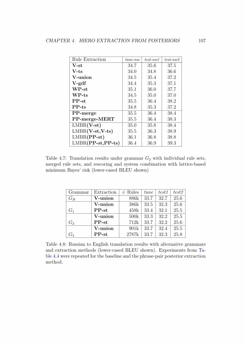
CHAPTER 4. HIERO EXTRACTION FROM POSTERIORS 107
Rule Extraction tune-nw test-nw1 test-nw2V-st 34.7 35.6 37.5V-ts 34.0 34.8 36.6V-union 34.5 35.4 37.2V-gdf 34.4 35.3 37.1WP-st 35.1 36.0 37.7WP-ts 34.5 35.0 37.0PP-st 35.5 36.4 38.2PP-ts 34.8 35.3 37.2PP-merge 35.5 36.4 38.4PP-merge-MERT 35.5 36.4 38.3LMBR(V-st) 35.0 35.8 38.4LMBR(V-st,V-ts) 35.5 36.3 38.9LMBR(PP-st) 36.1 36.8 38.8LMBR(PP-st,PP-ts) 36.4 36.9 39.3
Table 4.7: Translation results under grammar G2 with individual rule sets,merged rule sets, and rescoring and system combination with lattice-basedminimum Bayes’ risk (lower-cased BLEU shown)
Grammar Extraction # Rules tune test1 test2GH V-union 886k 33.7 32.7 25.6
V-union 386k 33.5 32.3 25.6G1 PP-st 458k 33.4 32.1 25.5
V-union 500k 33.3 32.2 25.5G2 PP-st 712k 33.7 32.2 25.6
V-union 901k 33.7 32.4 25.5G3 PP-st 2787k 33.7 32.3 25.8
Table 4.8: Russian to English translation results with alternative grammarsand extraction methods (lower-cased BLEU shown). Experiments from Ta-ble 4.4 were repeated for the baseline and the phrase-pair posterior extractionmethod.

CHAPTER 4. HIERO EXTRACTION FROM POSTERIORS 108
with differences in the order of 0.1 BLEU. We hypothesise that because thereis less reordering between Russian and English, the quality of the Viterbialignments, therefore the quality of the rules extracted, is high enough toalready produce relatively high quality translations.
4.5 ConclusionWe have presented new rule extraction methods that lead to larger rule setsas well as better estimated translation models. In Chinese-English trans-lation experiments, a simple grammar estimated with these methods wasshown to outperform a baseline hierarchical grammar extracted from Viterbialignments. A fine-grained analysis was provided to explain the advantagesof the phrase-pair posterior extraction method. Finally, it was shown thatthe best way to exploit both alignment directions is to train separate mod-els for each direction, translate separately and combine the lattice outputs.In addition, the same techniques were explored in the context of Russian-English translation and provided the same translation quality as the baselinetechnique.

Chapter 5
Domain Adaptation forHierarchical Phrase-BasedTranslation Systems
In Chapter 3, we have demonstrated improvements in scalability for genera-tion of and retrieval from hierarchical phrase-based grammars. In Chapter 4,we have introduced an original model for hierarchical phrase-based gram-mar extraction and estimation. In this chapter, we will investigate furtherrefinements for hierarchical phrase-based grammar modelling in the contextof domain adaptation. We will also investigate possible improvements forlanguage modelling both in the context of domain adaptation and in termsof training data size.
5.1 IntroductionAs described in Section 1.2.1, SMT state-of-the-art systems consist of apipeline of various modules. These modules interact in complex ways, whichmakes experimentation challenging, but also provides an opportunity to makeimprovements in separate modules with the hope that the end-to-end sys-tem will be improved overall. In this chapter, we describe investigationsinto language model and grammar refinement techniques for SMT. We com-pare various strategies for grammar and language modelling in the contextof domain adaptation. We also explore the interaction between a first passlanguage model used in decoding and a second pass language model used in
109

CHAPTER 5. HIERO DOMAIN ADAPTATION 110
rescoring. Finally, we compare two smoothing strategies for large languagemodel rescoring. The techniques presented in this chapter may be used in or-der to build high quality systems for a translation evaluation or to customisea translation system for a client in the industry setting. Figure 5.1 indicateswhich modules we attempt to improve.
Experiments are based on a system submitted to the WMT13 Russian-English translation shared task (Pino et al., 2013). Because we developed avery competitive system for this evaluation, refinements on that system give agood indication of which techniques are worthwhile applying to SMT systems.We briefly summarise the system building in Section 5.2. In Section 5.3, wereview domain adaptation techniques for machine translation. In Section 5.4,we show how to adapt a language model to obtain better performance on aspecific domain such as newswire text. In Section 5.5, we show how additionalgrammar rule features related to specific domains may help in translation.In Section 5.6, we investigate the various strategies for combining first passtranslation and language model rescoring in terms of language model trainingdata size and n-gram language model order. Finally, in Section 5.7, wecompare two smoothing strategies for large language model rescoring.
5.2 Description of the System to be DevelopedThe experiments reported in this chapter are based on the system submittedto the WMT13 Russian-English translation shared task (Pino et al., 2013). 19systems were submitted to this particular task. The CUED system obtainedthe best case-sensitive BLEU score and the second best human judgementscore amongst constrained-track systems (Bojar et al., 2013).1 In this section,we summarise the system building.
We use all the Russian-English parallel data available in the constrainedtrack. We filter out non Russian-English sentence pairs with the language-detection library.2 A sentence pair is filtered out if the language detectordetects a different language with probability more than 0.999995 in eitherthe source or the target. This discards 78,543 sentence pairs from an initial2,543,462. For example, the sentence in Figure 5.2 was detected as Frenchwith a probability of 0.999997. In addition, sentence pairs where the sourcesentence has no Russian character, defined by the Perl regular expression
1 http://matrix.statmt.org/matrix/systems_list/17382 http://code.google.com/p/language-detection/
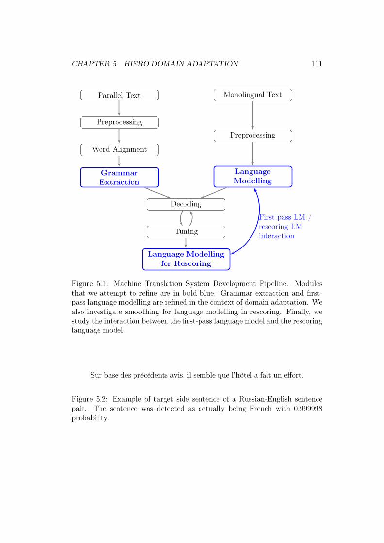
CHAPTER 5. HIERO DOMAIN ADAPTATION 111
..Parallel Text.
Preprocessing
.
Word Alignment
.
GrammarExtraction
. Monolingual Text.
Preprocessing
.
LanguageModelling
..
Decoding
.
Tuning
.
Language Modellingfor Rescoring
.
First pass LM /rescoring LMinteraction
Figure 5.1: Machine Translation System Development Pipeline. Modulesthat we attempt to refine are in bold blue. Grammar extraction and first-pass language modelling are refined in the context of domain adaptation. Wealso investigate smoothing for language modelling in rescoring. Finally, westudy the interaction between the first-pass language model and the rescoringlanguage model.
Sur base des precedents avis, il semble que l’hotel a fait un effort.
Figure 5.2: Example of target side sentence of a Russian-English sentencepair. The sentence was detected as actually being French with 0.999998probability.

CHAPTER 5. HIERO DOMAIN ADAPTATION 112
[\x0400-\x04ff], are discarded. This regular expression corresponds to theUnicode block for Cyrillic characters (in hexadecimal notation, code 0400 tocode 04ff). This further discards 19000 sentence pairs. We take the view thatdiscarding a small portion of training data in order to obtain cleaner data isbeneficial in translation, when such cues are easily and reliably available.
The Russian side of the parallel corpus is tokenised with the StanfordCoreNLP toolkit.3 The English side of the parallel corpus is tokenised witha standard English tokeniser, which splits sentences into tokens using whitespace and punctuation, and retains abbreviations as single tokens. Both sidesof the parallel corpus are then lowercased. Corpus statistics after filteringand tokenisation are summarised in Table 5.1.
Language # Tokens # TypesRU 47.4M 1.2MEN 50.4M 0.7M
Table 5.1: Russian-English parallel corpus statistics after filtering and to-kenisation. Parallel text contains approximately 50M tokens on each side.This translation task can be characterised as a medium size translation task.
Parallel data is aligned using the MTTK toolkit (Deng and Byrne, 2008):we train a word-to-phrase HMM model with a maximum phrase length of 4in both source-to-target and target-to-source directions (see Section 2.3.1).The final alignments are obtained by taking the union of alignments obtainedin both directions. A hierarchical phrase-based grammar is extracted fromthe alignments as described in Section 3.4. The constraints for extractiondescribed in Section 3.5.2 are set as follows:
• smax = 9 (maximum number of source terminals for phrase-based rules)
• smax elements = 5 (maximum number of source terminals and nontermi-nals)
• smax terminals = 5 (maximum number of source consecutive terminals)
• smax NT = 10 (maximum source nonterminal span)3 http://nlp.stanford.edu/software/corenlp.shtml

CHAPTER 5. HIERO DOMAIN ADAPTATION 113
We are using a shallow-1 hierarchical grammar (see Section 2.6.2.4) in ourexperiments. This model is constrained enough that the decoder can buildexact search spaces, i.e. there is no pruning in search that may lead to searcherrors under the model.
We use the KenLM toolkit (Heafield et al., 2013) to estimate a singlemodified Kneser-Ney smoothed 4-gram language model (see Section 2.7.3) onall available monolingual data available in the constrained track. Statisticsfor the monolingual data are presented in Table 5.2.
Corpus # TokensEU + NC + UN + CzEng + Yx 652.5MGiga + CC + Wiki 654.1MNews Crawl 1594.3Mafp 874.1Mapw 1429.3Mcna + wpb 66.4Mltw 326.5Mnyt 1744.3Mxin 425.3MTotal 7766.9M
Table 5.2: Statistics for English monolingual corpora used to train lan-guage models. Abbreviations are used for the following corpora: Europarl(EU), News Commentary (NC), United Nations (UN), Czech-English corpus(CzEng), Yandex (Yx), 109 French-English corpus (Giga), Common Crawl(CC), Wikipedia Headlines (Wiki). Corpora “afp” and below are the variousnews agency from the GigaWord corpus.
For first-pass decoding, we use HiFST as described in Section 2.9. First-pass decoding is followed by a large 5-gram language model rescoring step asdescribed in Section 2.10. The 5-gram language model also uses all availablemonolingual data described in Table 5.2.
Two development sets are available: newstest2012 with 3003 sentencesand newstest2013 with 3000 sentences. We extract odd numbered sentencesfrom newstest2012 in order to obtain a tuning set newstest2012.tune. Evennumbered sentences from newstest2012 form a test set newstest2012.test.The newstest2013 set is used as an additional test set. newstest2012.tune,

CHAPTER 5. HIERO DOMAIN ADAPTATION 114
Configuration tune test1 test2baseline 1st pass 33.22 32.01 25.35baseline +5g 33.33 32.26 25.53
Table 5.3: WMT13 Russian-English baseline system. Performance is mea-sured by case-insensitive BLEU. The 1st pass configuration indicates resultsobtained after decoding. The +5g configuration indicates results obtainedafter 5-gram language model rescoring.
newstest2012.test and newstest2013 are respectively shortened to tune, test1and test2.
We report our baseline experiment in Table 5.3. We indicate case-insensitiveBLEU score after first-pass decoding and 5-gram language model rescoring.We will now investigate various strategies in order to improve performanceover the baseline. We will investigate domain adaptation techniques in orderto estimate better language models and grammars for translating newswiredata. We will also study the interaction between the first-pass languagemodel and the rescoring language model. Finally, we will study an alterna-tive smoothing technique to Stupid Backoff for the rescoring language model.
5.3 Domain Adaptation for Machine Transla-tion
In this section, we first introduce in Section 5.3.1 the general problem ofdomain adaptation and how certain machine translation settings may beinstances of this problem. We then review previous work on addressing theproblem of domain adaptation in SMT in Section 5.3.2.
5.3.1 Domain Adaptation
Let us first formalise the problem of domain adaptation. In a standard multi-class classification problem, we are given a training set {(xi, yi) ∈ X ×Y , i ∈[1, N ]} where X is a set of instances to be labelled and Y is a finite set oflabels. The multi-class classification learning problem is to find a functionf : X → Y that minimises the number of prediction errors. Machine transla-tion can be seen as a multi-class classification problem where X is the set of

CHAPTER 5. HIERO DOMAIN ADAPTATION 115
In addition, a new seven-year EU budget needs to be passed,which is very complicated due to the current crisis.
Figure 5.3: Example of English sentence in the newswire domain.
all possible source sentences and Y is the set of all possible target sentences.The multi-class classification framework is not very intuitive for machinetranslation. First, at least in theory, there are an infinite number of possibletarget sentences to choose from in translation. In addition, many possibletranslations are correct or acceptable in general. However, the multi-classclassification setting is assumed by the original objective function (see Sec-tion 2.2), which we recall in Equation 5.1. This objective function minimisesthe number of misclassifications.
e = argmaxe
p(e | f) (5.1)
A domain is a particular distribution D over X . For example, D can besuch that source sentences in X drawn from D are in the newswire domain.For example, if source sentences are in English, then source sentences drawnsampled from X with distribution D may look like the sentence in Figure 5.3.
For domain adaptation, we assume an out-of-domain distribution DO anda in-domain distribution DI . A model is trained on a sample drawn from DO
but the model performance is evaluated on a sample drawn from DI . Domainadaptation consists in altering the training procedure by using informationfrom domain DI in order to achieve better performance on DI . The out-of-domain and in-domain distributions are also called source domain andtarget domain respectively. A simple example of domain adaptation settingfor SMT may be that the parallel text is a parallel corpus of tweets4 andsentences to be translated come from newspaper articles.
5.3.2 Previous Work on Domain Adaptation for SMT
In machine translation, we can distinguish two types of domain adapta-tion problem: cross-domain adaptation and dynamic adaptation (Foster and
4 https://twitter.com/
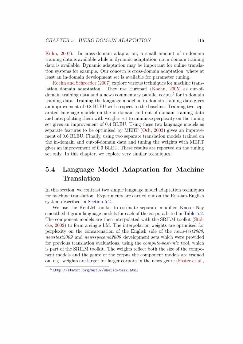
CHAPTER 5. HIERO DOMAIN ADAPTATION 116
Kuhn, 2007). In cross-domain adaptation, a small amount of in-domaintraining data is available while in dynamic adaptation, no in-domain trainingdata is available. Dynamic adaptation may be important for online transla-tion systems for example. Our concern is cross-domain adaptation, where atleast an in-domain development set is available for parameter tuning.
Koehn and Schroeder (2007) explore various techniques for machine trans-lation domain adaptation. They use Europarl (Koehn, 2005) as out-of-domain training data and a news commentary parallel corpus5 for in-domaintraining data. Training the language model on in-domain training data givesan improvement of 0.8 BLEU with respect to the baseline. Training two sep-arated language models on the in-domain and out-of-domain training dataand interpolating them with weights set to minimise perplexity on the tuningset gives an improvement of 0.4 BLEU. Using these two language models asseparate features to be optimised by MERT (Och, 2003) gives an improve-ment of 0.6 BLEU. Finally, using two separate translation models trained onthe in-domain and out-of-domain data and tuning the weights with MERTgives an improvement of 0.9 BLEU. These results are reported on the tuningset only. In this chapter, we explore very similar techniques.
5.4 Language Model Adaptation for MachineTranslation
In this section, we contrast two simple language model adaptation techniquesfor machine translation. Experiments are carried out on the Russian-Englishsystem described in Section 5.2.
We use the KenLM toolkit to estimate separate modified Kneser-Neysmoothed 4-gram language models for each of the corpora listed in Table 5.2.The component models are then interpolated with the SRILM toolkit (Stol-cke, 2002) to form a single LM. The interpolation weights are optimised forperplexity on the concatenation of the English side of the news-test2008,newstest2009 and newssyscomb2009 development sets which were providedfor previous translation evaluations, using the compute-best-mix tool, whichis part of the SRILM toolkit. The weights reflect both the size of the compo-nent models and the genre of the corpus the component models are trainedon, e.g. weights are larger for larger corpora in the news genre (Foster et al.,
5 http://statmt.org/wmt07/shared-task.html

CHAPTER 5. HIERO DOMAIN ADAPTATION 117
Row Configuration tune test1 test21 baseline 1st pass 33.22 32.01 25.352 baseline +5g 33.33 32.26 25.533 linear 1st pass 33.71 32.26 25.474 linear +5g 33.74 32.51 25.585 loglinear 1st pass 33.23 31.75 25.376 loglinear +5g 33.28 31.85 25.48
Table 5.4: Performance comparison, measured by case-insensitive BLEU, be-tween an uninterpolated language model (baseline), a linearly interpolatedlanguage model (linear) and a log-linearly interpolated language model (log-linear). Off-line linear interpolation (rows 3 and 4) is the best strategy.The loglinear configuration performs worst, however this may be due to theMERT optimisation algorithm not being able to find a high quality set ofparameters with 20 features.
2013). Thus we obtain a linear mixture of language models. We call thisconfiguration “linear”. As a contrast, we also keep the individual languagemodels as separate features in optimisation. We call this configuration “log-linear”.
We compare the baseline, the linear and the loglinear configurations inTable 5.4. We observe that the best strategy for building a language modelis to do offline linear interpolation to minimise perplexity on a developmentset that has the same genre as the translation test sets (row 3). The secondbest strategy is to use an uninterpolated language model (row 1). The worststrategy is to do a log-linear interpolation of the various language modelcomponents by tuning these language language models as separate featureswith lattice MERT (row 5). Note that these observations are confirmed evenafter rescoring with a large Stupid Backoff 5-gram language model (rows 2,4 and 6). It is possible that the loglinear configuration, which has 20 fea-tures as opposed to 12 features for the baseline and the linear configuration,performs worst because the MERT algorithm becomes unstable with morefeatures (Foster and Kuhn, 2009). These results are in contrast to thoseobtained previously (Koehn and Schroeder, 2007), where the loglinear inter-polation was found to provide more benefits over the linear interpolation. Inaddition, more language models are considered (9 vs. 2). Finally, both tuneand test results are reported here.
CHAPTER 5. HIERO DOMAIN ADAPTATION 118
5.5 Domain Adaptation with Provenance Fea-tures
In Section 5.4, we have presented domain adaptation strategies for the lan-guage model. In this section, we will focus on domain adaptation for thetranslation model. Chiang et al. (2011) introduce provenance lexical fea-tures. The concept of provenance was introduced previously (Matsoukaset al., 2009) and provides metadata information such as genre or collectionfor each sentence pair in parallel text. Word translation tables and lexicalfeatures are computed for each provenance. Finally, for each provenance, theratio of the provenance specific lexical feature with the global lexical featureis added as a feature to the translation system.
We use a very similar approach with the following differences and exten-sions:
• The lexical features are computed with Model 1 rather than Viterbialignments, as described in Section 2.6.5.
• The features added to the system are not the ratios between a prove-nance specific lexical feature and the global lexical feature but simplythe provenance specific lexical features.
• We extend this technique to compute provenance specific source-to-target and target-to-source translation models as described in Sec-tion 3.4.
For our experiments, we use 4 provenances that correspond to the 4 sub-corpora provided for parallel text: the Common Crawl corpus, the NewsCommentary corpus, the Yandex corpus and the Wiki Headlines corpus.This gives an additional 16 features to our system: source-to-target andtarget-to-source translation and lexical features for each provenance. Thisconfiguration is called “provenance”.
When retrieving relevant rules for a particular test set, various thresholdsare applied, such as number of targets per source or translation probabilitycutoffs. Thresholds involving source-to-target translation scores are appliedseparately for each provenance and the union of all surviving rules for eachprovenance is kept. This configuration is called “provenance union”. Thisspecific configuration was used for submission to the translation task com-petition at WMT13. To our knowledge, this original technique has not been

CHAPTER 5. HIERO DOMAIN ADAPTATION 119
Row Configuration tune test1 test21 no provenance 1st pass 33.71 32.26 25.472 no provenance +5g 33.74 32.51 25.583 provenance 1st pass 33.22 32.14 25.404 provenance +5g 33.22 32.14 25.415 provenance union 1st pass 33.65 32.36 25.556 provenance union +5g 33.67 32.58 25.637 no provenance union 1st pass 33.22 31.78 25.598 no provenance union +5g 33.22 31.78 25.59
Table 5.5: Effect of using provenance features. Case-insensitive BLEU scoresare reported. The most effective strategy is provenance union. Because the“no provenance union” does not improve over the baseline, we conclude thatthe gains obtained by the provenance union strategy are not only due toadditional rules; instead, they are due to the conjunction of additional ruleswith provenance features for better discrimination.
employed previously. Results show that it provides additional gains over thesimple use of provenance features.
The first-pass language model is the linear mixture described in Sec-tion 5.4. We also compare the various configurations after 5-gram rescoring.Results are presented in Table 5.5. We can see that adding provenance fea-tures slightly degrades performance (row 3 vs. row 1, row 4 vs. row 2). Thisagain may be due to the inability of the MERT optimisation algorithm totune more than the 12 basic features. However, if we use the provenanceunion strategy, we can see that having additional rules together with prove-nance features is the best strategy (row 5 vs. row 1, row 6 vs. row 2). Inorder to verify whether the gains are only due to additional rules, we rerun theexperiment with the provenance union configuration but remove the prove-nance features (row 7 and row 8). The performance of the “no provenanceunion” configuration is worse or equal to the “no provenance” configuration,which demonstrates that the provenance union strategy is optimal in this setof experiments and that the gains provided are not only due to having addi-tional translation rules. The effectiveness of the provenance union strategyis due to additional rules in conjunction with additional features for betterdiscrimination between rules.

CHAPTER 5. HIERO DOMAIN ADAPTATION 120
5.6 Interaction between First Pass LanguageModel and Rescoring Language Model
In Section 5.4 and Section 5.5, we have investigated various strategies toadapt the language model and translation model to the genre of the testset to be translated. In each case, we verified that the conclusions heldeven after rescoring with a large 5-gram language model. In this section, westudy the interaction between the first pass language model and the rescoringlanguage model in terms of n-gram order and training data size. We giverecommendations on how much data should be used to train a first passlanguage model and what order should be chosen for the first pass n-gramlanguage model.
Our translation systems are typically run in two steps. The first stepusually consists in decoding with a 4-gram language model. The second stepconsists in 5-gram lattice rescoring. Brants et al. (2007) argue that singlepass decoding is conceptually simpler and may lose less information. In thissection, we also attempt to verify this claim by incorporating 5-gram languagemodels directly in first-pass decoding and evaluate performance with respectto a two-pass strategy.
We describe the various configurations used for experiments and reportedin Table 5.6. For monolingual data size, we use a “large” configuration whichuses all available data described in Table 5.2, and a “medium” configurationwhich uses the following corpora: EU, NC, UN, CzEng, Yx, Giga, CC, Wiki,afp and xin. (The keys for abbreviations are described in Table 5.2). Wealso train 4-gram and 5-gram language models with large and medium datafor the first pass language model. The “large 4g” configuration correspondsto the linear configuration from Table 5.4.
The initial parameter for the MERT optimisation step was the same forall configurations. This parameter was obtained from a separate Arabic-to-English experiment carried out earlier. Reusing already optimised parame-ters between experiments allows us to do faster experimentation since lessiterations are needed until convergence.
Results are presented in Table 5.6. Comparing row 1 and row 3, we cansee that for a 4-gram language model, more training data is beneficial infirst-pass decoding. This conclusion is confirmed after 5-gram rescoring (row2 vs. row 4). However, when comparing row 5 vs. row 7 and row 6 vs. row8, we conclude that in the case of a first-pass 5-gram language model, more
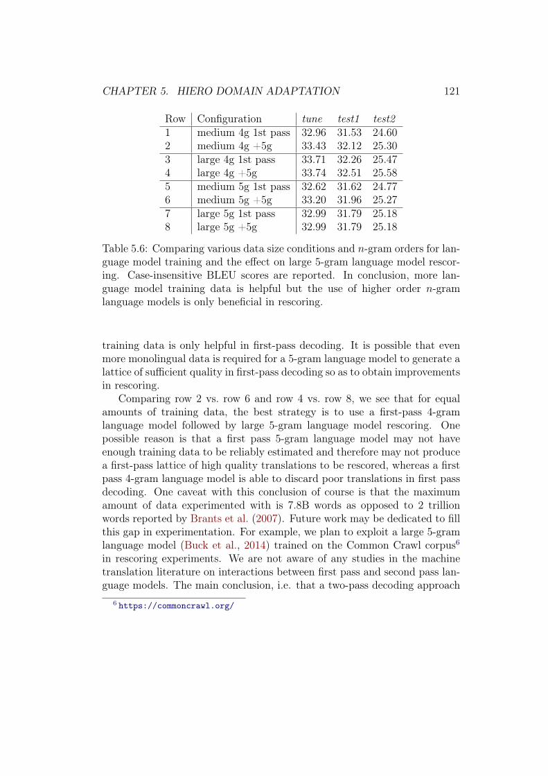
CHAPTER 5. HIERO DOMAIN ADAPTATION 121
Row Configuration tune test1 test21 medium 4g 1st pass 32.96 31.53 24.602 medium 4g +5g 33.43 32.12 25.303 large 4g 1st pass 33.71 32.26 25.474 large 4g +5g 33.74 32.51 25.585 medium 5g 1st pass 32.62 31.62 24.776 medium 5g +5g 33.20 31.96 25.277 large 5g 1st pass 32.99 31.79 25.188 large 5g +5g 32.99 31.79 25.18
Table 5.6: Comparing various data size conditions and n-gram orders for lan-guage model training and the effect on large 5-gram language model rescor-ing. Case-insensitive BLEU scores are reported. In conclusion, more lan-guage model training data is helpful but the use of higher order n-gramlanguage models is only beneficial in rescoring.
training data is only helpful in first-pass decoding. It is possible that evenmore monolingual data is required for a 5-gram language model to generate alattice of sufficient quality in first-pass decoding so as to obtain improvementsin rescoring.
Comparing row 2 vs. row 6 and row 4 vs. row 8, we see that for equalamounts of training data, the best strategy is to use a first-pass 4-gramlanguage model followed by large 5-gram language model rescoring. Onepossible reason is that a first pass 5-gram language model may not haveenough training data to be reliably estimated and therefore may not producea first-pass lattice of high quality translations to be rescored, whereas a firstpass 4-gram language model is able to discard poor translations in first passdecoding. One caveat with this conclusion of course is that the maximumamount of data experimented with is 7.8B words as opposed to 2 trillionwords reported by Brants et al. (2007). Future work may be dedicated to fillthis gap in experimentation. For example, we plan to exploit a large 5-gramlanguage model (Buck et al., 2014) trained on the Common Crawl corpus6
in rescoring experiments. We are not aware of any studies in the machinetranslation literature on interactions between first pass and second pass lan-guage models. The main conclusion, i.e. that a two-pass decoding approach
6 https://commoncrawl.org/

CHAPTER 5. HIERO DOMAIN ADAPTATION 122
is beneficial over a single-pass approach given the amount of training data,has not been demonstrated experimentally before.
5.7 Language Model Smoothing in LanguageModel Lattice Rescoring
In Section 5.6, we have given recommendations about what strategy to adoptin first-pass decoding in order to obtain optimal results in rescoring. Theconclusion was to use a 4-gram language model trained on large amountsof data. In this section, we attempt to improve on the 5-gram rescoringprocedure by exploring two alternative smoothing strategies for the 5-gramlanguage model used for rescoring.
We train a Stupid Backoff 5-gram language model (see Section 2.7.4 andSection 3.2.1) and a modified Kneser-Ney 5-gram language model on all avail-able English data for WMT13, described in Table 5.2. We compare the twosmoothing methods in rescoring over various configurations used throughoutthis chapter. We did not include the “provenance union no provenance” andthe “large 5g” configurations. On average, over the seven experiments fromTable 5.7, we obtain a gain of 0.11 BLEU on the tuning set tune, a gain of0.14 BLEU on the first test set test1 and a gain of 0.13 BLEU on the secondtest set test2. We conclude that the use of modified Kneser-Ney smoothingis slightly beneficial in 5-gram lattice rescoring when the amount of train-ing data is in the order of several billion tokens. This confirms conclusionsfrom Figure 5 in a previous publication (Brants et al., 2007) that Kneser-Neysmoothing is superior to Stupid Backoff smoothing with amounts of train-ing data in a similar order to the work here. These conclusions were madefor first pass decoding while here. This is the first time these two smooth-ing strategies are compared in the context of 5-gram language model latticerescoring. We also note that we obtain an improvement over the system sub-mitted to the WMT13 translation task using the “provenance union + KN5g” configuration (row 15 in bold vs. row 14).
5.8 ConclusionIn this chapter, we have investigated various refinements on translation sys-tem building. We have explored domain adaptation techniques in order to

CHAPTER 5. HIERO DOMAIN ADAPTATION 123
Row Configuration tune test1 test21 baseline 1st pass 33.22 32.01 25.352 baseline + SB 5g 33.33 32.26 25.533 baseline + KN 5g 33.31 32.28 25.654 linear 1st pass 33.71 32.26 25.475 linear + SB 5g 33.74 32.51 25.586 linear + KN 5g 33.73 32.26 25.487 loglinear 1st pass 33.23 31.75 25.378 loglinear + SB 5g 33.28 31.85 25.489 loglinear + KN 5g 33.30 31.92 25.3510 provenance 1st pass 33.22 32.14 25.4011 provenance + SB 5g 33.22 32.14 25.4112 provenance + KN 5g 33.54 32.37 25.7513 provenance union 1st pass 33.65 32.36 25.5514 provenance union + SB 5g 33.67 32.58 25.6315 provenance union + KN 5g 33.89 32.82 25.8416 medium 5g 1st pass 32.62 31.62 24.7717 medium 5g + SB 5g 33.20 31.96 25.2718 medium 5g + KN 5g 33.24 32.29 25.4719 medium 4g 1st pass 32.96 31.53 24.6020 medium 4g + SB 5g 33.43 32.12 25.3021 medium 4g + KN 5g 33.65 32.46 25.55
Table 5.7: Comparison between the gains obtained by Stupid Backoff 5-gram rescoring and Kneser-Ney 5-gram rescoring. Case-insensitive BLEUscores are reported. In conclusion, at the level of several billion tokens forlanguage model training, Kneser-Ney smoothing is beneficial over StupidBackoff smoothing in the context of 5-gram lattice rescoring. Row 15 (inbold) achieves a better performance than row 14, which was our systemsubmitted to the WMT13 translation shared task.

CHAPTER 5. HIERO DOMAIN ADAPTATION 124
refine the language model and the translation model. For language modelbuilding, we find that the best strategy for cross-domain adaptation is tobuild an interpolated language model and tune the interpolation weights inorder to minimise the perplexity on a development set in the target domain,as opposed to tuning the language model weights with MERT. We also haveexamined the effect of provenance features in the translation model. Wefound that the use provenance features is beneficial only when these featuresare used to discriminate rules from a larger rule set.
After having attempted to refine models used in first-pass decoding, wehave studied the interaction between the first pass language model and the5-gram language model used in lattice rescoring. We have come to the con-clusion that in our setting, a two-pass strategy is preferable and that usinglarge amounts of data to train a 4-gram language model for first-pass decod-ing yields better results in rescoring.
Finally, we have demonstrated that Kneser-Ney smoothing produces bet-ter results than Stupid Backoff smoothing when training a 5-gram languagemodel on 7.8 billion words for rescoring purposes. This confirms previousresearch in the context of rescoring as opposed to first-pass decoding.

Chapter 6
String Regeneration asPhrase-Based Translation
In the previous chapters, we have proposed various improvements to hier-archical phrase-based translation systems, in terms of infrastructure (Chap-ter 3), grammar modelling (Chapter 4 and Chapter 5) and language mod-elling for first pass decoding as well as rescoring (Chapter 5). In the chapterto follow (Chapter 7), we will also introduce techniques for potential improve-ments in fluency in the output of hierarchical phrase-based systems. In thischapter, we lay the ground work to be applied in translation in Chapter 7.
Machine translation output was originally evaluated by human judges interms of adequacy, or how well the meaning of the source text is preserved inthe translated text, and fluency, or how well-formed the translation is (Whiteet al., 1993), i.e. to what extent it is syntactically, morphologically, and ortho-graphically correct (Reiter and Dale, 1997). Adequacy and fluency motivatethe separation of SMT models into a translation model and a language model(see Section 2.2). There is increasing concern that translation output oftenlacks fluency (Knight, 2007). In this chapter, we study the related prob-lem of string regeneration: given a sentence where the word order has beenscrambled, how difficult is it to recover the original sentence ? Our approachis inspired by phrase-based translation techniques and achieves state-of-the-art performance on the string regeneration task. Software written for thischapter is available online.1
1 https://github.com/jmp84/NgramGen
125
CHAPTER 6. STRING REGENERATION AS PHRASE-BASED MT 126
6.1 IntroductionBefore the widespread use of automatic metrics such as BLEU (see Sec-tion 2.8.1) or METEOR (Banerjee and Lavie, 2005), machine translationsystems were originally evaluated in terms of adequacy and fluency. Currentpopular automatic metrics for translation can be “gamed” in the sense that itis possible to obtain a high score according to these metrics with an outputthat lacks fluency. For example, a translation may obtain a high BLEU scoresimply because it contains many n-grams that are also in the reference trans-lation but this translation may not be well-formed syntactically. Figure 6.1shows how an improvement of 20 BLEU points at the sentence level betweenan MT hypothesis and an oracle MT hypothesis, i.e. the best performinghypothesis among a set, may not translate into an improvement in fluency.Of course, BLEU is designed to measure quality at the set level, so hopefullyother oracle MT hypotheses will probably improve fluency. The nature of thetranslation metrics may have led research on translation to neglect fluency.
Correct word ordering is an essential part of fluency. Producing a trans-lation with words correctly ordered is a very difficult task. Different wordordering between distant language pairs such as Chinese-English is one of themain reasons for incorrect word ordering in translation. In general, obtain-ing a correct word order is a fundamental problem in many natural languageprocessing applications. In machine translation, because source language andtarget language have a different word ordering, a machine translation systemneeds to model word reordering. In some language pairs such as French-English, the source language gives good cues to the target word order; how-ever, in other language pairs such as Chinese-English or Japanese-English,the word order can be very different in the source and the target language.In natural language generation tasks, such as paraphrasing or summarisa-tion, word ordering is also critical at the surface realisation step (Reiter andDale, 1997). Word ordering is also one possible type of grammatical error,especially for foreign language learners (Yu and Chen, 2012).
In this chapter, we study the word ordering problem in isolation throughthe task of string regeneration (Wan et al., 2009). Given an input sentencewhere the word order has been scrambled, the string regeneration task con-sists in recovering the original sentence. This task can be seen as one of thesteps in surface realisation for language generation where the input is a listof content words and function words and the output a grammatical sentence.It also allows us to study the realisation task independently of the transla-

CHAPTER 6. STRING REGENERATION AS PHRASE-BASED MT 127
SMT System (19.76 Sentence-Level BLEU): enda accord-ing to jerzy made a televised speech, the president of burundi civilwar of resistance army soldiers in the past ten years, and had tosettle on january 5 before the completion of the new militaryleadership will be in place before january 7, four of the formerrebel army leader.
SMT System Oracle (39.91 Sentence-Level BLEU): en, aus $according to al made a televised speech, said that the presi-dent of the burundi’s rebel army soldiers in the past 10-year civilwar must be before january 5 and the completion of the new mil-itary leadership will be in place by january 7, and four of theformer leaders of the rebel forces.
Reference: According to President Ndayizeye’s televised speech,former rebel fighters in Burundi’s 10-year civil war must be settledin by January 5. The new army leadership is to be made up of40 percent former rebels and should be in place by January 7.
Figure 6.1: Example showing how a large improvement in BLEU score doesnot imply an improvement in fluency. The first quote is one of the outputsentences produced by an SMT system presented in Chapter 7. The secondquote is the oracle translation for that system, i.e. the best possible transla-tion to be found in the lattice of translations generated by the system. Thethird quote is one of the human reference translations. Note that the oraclehypothesis was picked to maximise sentence-level BLEU, which shows that,in principle, it is possible to obtain a translation with a high BLEU scorebut that lacks fluency.
CHAPTER 6. STRING REGENERATION AS PHRASE-BASED MT 128
tion task. Finally, it can have alternative applications such as automaticallyproducing alternative references for machine translation.
We use a simple but extensible approach, inspired from stack-based de-coding for phrase-based translation (see Section 2.5.4). Given a bag of wordsas input, we use n-gram rules extracted from a large monolingual corpus andconcatenate these n-grams in order to form hypotheses. The hypotheses arescored with a linear model in the same manner as translation hypotheses inphrase-based translation. One of the critical features in this system is thelanguage model. In experiments to follow, we only study this main languagemodel feature, however, our decoder has other features implemented and ar-bitrary features can be added easily to the system, demonstrating the systemflexibility.
Our strategy achieves state-of-the-art performance as measured by BLEU(Section 2.8.1) in the string regeneration task. We also study various capa-bilities of our decoder: in Section 2.5.4, we show how to split the input intochunks for more rapid experimentation; in Section 6.6.4, we analyse the ef-fect of stack-based pruning; in Section 6.6.5, we study the effect of includingn-gram rules with a larger n-gram order; in Section 6.6.6, we relax decodingconstraints by allowing n-gram rules to overlap; in Section 6.6.7, we intro-duce future cost estimation using a unigram language model; finally, in Sec-tion 6.6.8, we demonstrate how SMT rescoring techniques are also applicableto the output of our decoder.
6.2 BackgroundBrown et al. (1990) anecdotally mention the string regeneration task, or bagof words translation, in order to demonstrate the effectiveness of n-gramlanguage models. With a 3-gram language model, they recover 63% of a sen-tences with less than 11 words with brute force search over all permutations.This is of course impractical for longer sentences.
String regeneration has recently gained interest as a standalone task.Wanet al. (2009) introduced the string regeneration task as a proxy to measurethe grammaticality of a natural language generation system output. Stringregeneration can also be considered as a simplified version of the linguisticrealisation task in a natural language generation system (Reiter and Dale,1997), which consists in generating a surface form that is syntactically, mor-phologically, and orthographically correct.

CHAPTER 6. STRING REGENERATION AS PHRASE-BASED MT 129
Wan et al. (2009) use a modified version of the minimum spanning treealgorithm in order to find an optimal dependency tree that covers an inputbag of words. Once a dependency tree is built, an n-gram language modelis used so as to order siblings in the tree. Performance is measured by theBLEU metric. Wan et al. (2009) demonstrate BLEU improvements whenregenerating Section 23 of the Penn Treebank using their original algorithmvs. baseline algorithms based on n-gram language models only. Base nounsindicated by the Penn Treebank are kept together for experimentation.
He et al. (2009) also use the dependency tree formalism for string real-isation. They describe a sentence realiser that takes as input an unordereddependency tree, i.e. a dependency tree that only encode head-modifier re-lations but not the surface string ordering. Because an exhaustive searchis intractable (due to the number of possible children permutations at eachnode), He et al. (2009) adopt a divide-and-conquer approach that recursivelylinearises subtrees in a bottom-up fashion. A log-linear model is used toselect the best possible linearisation for each subtree. Features include de-pendency relations, n-gram language models for the surface string and forthe sequence of heads.
CCG grammars (Zhang and Clark, 2011) have also been used for thestring regeneration task as an alternative to the dependency grammar for-malism. Given an input bag of words, the best CCG parse that covers theinput is searched for. Similarly to previous work, input base nouns are keptas single units. In follow-up work (Zhang et al., 2012), CCG grammars arecombined with large language models and provide performance improvementsas measured by the BLEU metric.
Some of the works described so far are instances of tree linearisation:given a set of unordered dependencies, reconstruct a dependency tree whichgives the word ordering (Belz et al., 2012). Zhang (2013) extends this taskto partial tree linearisation: the input is a set of possibly missing POS tagsand possibly missing unordered dependencies. This last work achieves state-of-the art performance on string regeneration on the Penn Treebank, whenusing dependency information on the input. Zhang (2013) also reports resultson string regeneration without using dependency information on the inputbut keeping base noun phrases as single units.
In this chapter, we restrict the input to be a bag of words without anyadditional syntactic or semantic information. Our work is directly inspiredby recent work that exploits phrase-based grammars together with a hier-archical phrase-based decoder based on FSTs (see Section 2.9) (de Gispert
CHAPTER 6. STRING REGENERATION AS PHRASE-BASED MT 130
et al., 2014). We also use phrase-based grammars, but our decoding pro-cedure is analogous to stack-based decoding for phrase-based translation.To our knowledge, our method achieves state-of-the-art performance on thistask. We will now present our model, which is analogous to the phrase-basedtranslation model, but in a monolingual setting.
6.3 Phrase-Based Translation Model for StringRegeneration
In the previous section, we have reviewed various strategies for string regen-eration. We observe that, in general, the use of syntax was beneficial overthe exclusive use of an n-gram language model. We do not take advantage ofsyntactic information, instead, we complement an n-gram language with n-gram rules extracted from monolingual data. We now describe our method,which is inspired from phrase-based translation techniques (see Section 2.5).We employ a feature based linear model (see Section 2.4) as our objectivefunction:
e = argmaxe
λ · h(e) (6.1)
where:
• e is the best possible hypothesis according to the model.
• e is an English sentence.
• λ is a feature weight vector.
• h(e) is a feature vector for the hypothesis e.
Φ(e) contains a language model g(e) as well as local features ϕ(e) thatare additive over phrases that segment e. Similarly, λ has a weight λg forthe language model and weights λϕ for local features. As in phrase-basedtranslation, a hypothesis is decomposed into phrases eI
1. We can then rewriteEquation 6.1 into Equation 6.2:
e = argmaxe=eI1
λgg(e) + λϕ ·ϕ(e)
= argmaxe=eI1
λgg(e) + λϕ ·I∑
i=1
ϕ(ei)(6.2)
CHAPTER 6. STRING REGENERATION AS PHRASE-BASED MT 131
Note that this model makes a max approximation: various segmentationsof the hypotheses are considered but the score only depends on one singlesegmentation. Experiments to follow only make use of the language modelfeature but our implementation has other features integrated, such as wordcount or rule count, and arbitrary features can be added easily. Our decoderalgorithm described subsequently in Section 6.5 generates hypotheses left toright by concatenating phrases e1, ..., eI . For a phrase index i ∈ [1, I], wedefine the partial model score sc(ei
1) of partial hypothesis ei1 as in Equa-
tion 6.3:
sc(ei1) = λgg(e
i1) + λϕ ·
i∑k=1
ϕ(ek) (6.3)
6.4 Phrase-Based Translation Rules for StringRegeneration
In the previous section, we have introduced our model, inspired from phrase-based translation, for string regeneration. This model assumes that a hy-pothesis is segmented into phrases. In this section, we describe how to obtainthese phrases from monolingual data. In Section 6.4.1, we review the n-gramrule extraction process, which is based on the Hadoop implementation ofMapReduce. In Section 6.4.2, we describe how to obtain relevant rules for agiven test set.
6.4.1 Rule Extraction
n-gram rules are extracted from large collections of monolingual text. Thetext is tokenised and lowercased. We then employ the MapReduce frameworkas implemented by Hadoop in order to extract n-grams together with theiroccurrence counts from the corpus.
The input key to the map function is irrelevant. The input value to themap function is a line of text. The map function simply extracts all n-gramsfrom the input line of text and outputs these n-grams with a count of one.The input to the reduce function is an n-gram and a series of constant valuesequal to one. The reduce function simply sums the counts and producesthe n-gram with its total count. This MapReduce job is analogous to thecanonical “word count” example except that here n-grams of higher order

CHAPTER 6. STRING REGENERATION AS PHRASE-BASED MT 132
than unigrams are considered. For our experiments, we extract n-gramsfrom order 1 to 5.
6.4.2 Rule Filtering
Once we have extracted all n-grams from a monolingual corpus, we wouldlike to retrieve the n-grams relevant to a test set that we wish to experimenton. An n-gram is relevant if the vocabulary of the n-gram is included in anyof the vocabularies of each sentence in the test set.
Contrary to the process described in Section 3.5, we do not generatequeries and then seek those queries in an HFile. This is because the numberof possible queries is too large to fit in memory. For a sentence of length Nwith words distinct from each other, the number of possible relevant 5-gramsis N × (N − 1)× (N − 2)× (N − 3)× (N − 4). For sentence of length 100,this would correspond to approximately 9B queries. Even with an alternativeimplementation where keys in the HFile are lexicographically sorted n-gramsand values are the permutations and counts found in the monolingual data,the number of 5-gram queries would be
(N5
), which is approximately 75M
queries for a 100 word sentence.We therefore take the alternative approach of scanning the set of n-grams
and retaining the relevant ones. For this, we again use a MapReduce job. Theinput key to the map function is an n-gram and the input value is a count.For each test sentence, the map function checks if the n-gram vocabulary isincluded in the vocabulary of that sentence and if so, it generates all possiblecoverages of this n-gram for that sentence, where a coverage indicates thepositions of the words covered by the n-gram in the input sentence. The mapoutput key is the n-gram together with a sentence id. The map output valueis a coverage and a count. The reduce function simply removes duplicates inthe list of coverages.
6.5 String Regeneration SearchIn Section 6.3, we have described our string regeneration model and in Sec-tion 6.4, we have described how to extract n-gram rules. We now presentour search algorithm and introduce our string regeneration decoder, Ngram-Gen, which reorders an input bag of word using the model introduced andstack-based decoding techniques reviewed in Section 2.5.4.

CHAPTER 6. STRING REGENERATION AS PHRASE-BASED MT 133
6.5.1 Input
The input to the decoder consists of:
• A bag of words, or multiset, w, represented as a vector. For example,we have w = [do, you, do] for the input sentence “do you do” to beregenerated.
• A set of n-grams, where the vocabulary of each n-gram is a subset ofthe vocabulary of the input bag of words. Each n-gram is also associ-ated with one or more coverages as computed in Section 6.4.2. For agiven n-gram, its coverage is a bit vector that indicates what positionsthe n-gram covers in the input bag of words. In case of repeated words,an n-gram can have several possible coverages. For example, with theinput bag of words [do, you, do], the n-gram [do, you] has two possiblecoverages: 110 and 011. The input n-grams and coverages are repre-sented as an associative array datastructure. We denote this input byN . Note that it would be possible for the decoder to compute possiblecoverages on the fly, however we choose to precompute those at thefiltering step described in Section 6.4.2.
• A n-gram language model G. The n-gram language model is used as athe main feature in the model to encourage fluent output.
We will now describe how hypotheses, i.e. permutations of the input, aregenerated by the decoder from a bag of words.
6.5.2 Algorithm
Our algorithm is inspired by stack based decoding for phrase-based transla-tion, reviewed in Section 2.5.4. We first give an overview before outliningthe algorithm details.
6.5.2.1 Overview
In order to represent partial hypotheses, we use a vector of columns (morecommonly called stacks). Each column contains a set of states. Each staterepresents a set of partial hypotheses. All states in a column represent hy-potheses that cover the same number of words in the input.

CHAPTER 6. STRING REGENERATION AS PHRASE-BASED MT 134
We start to build hypotheses from an initial state that represents theempty hypothesis. This initial state is located in the first column, whichrepresents the hypotheses that have not covered any word in the input. Theempty hypothesis is then extended with the input n-gram rules and theircoverage. New states are created to take into account these extensions. Then,partial hypotheses represented by these states are repeatedly extended untilhypotheses that cover the entire input are produced.
6.5.2.2 Algorithm Details
As mentioned in Section 6.5.2.1, we represent the set of partial hypotheseswith a vector of columns that we denote M . For an input w of size |w|, Mhas a size of |w| + 1. Elements of M are denoted M0, ..., M|w|. The i-thcolumn Mi represents hypotheses that have covered i words in the input. Thecolumns Mi are the analog of stacks in stack based decoding for phrase-basedtranslation.
Each column contains a set of states that represents a set of partial hy-pothesis. A state contains the information necessary to extend a partialhypothesis and represents a set of partial hypotheses that can be recombined(see Section 2.5.4). This means that if two partial hypotheses h1 and h2 arerepresented by a state s and h1 has a higher model score than h2, then if h1
and h2 are extended with the same rules, then the extension of h1 will havea higher score than the extension h2. In our case, two hypotheses can berecombined if they share the same last n − 1 words where n is the order ofthe n-gram language model.
The states are sorted by their score. For a given state, its score is the bestmodel score of any of the partial hypotheses that the state represents. Thedecoding algorithm is presented in Figure 6.2. We first initialise the matrixM to be a vector of empty columns of size |w|+1 (line 2). The first columnis filled with an initial state representing an empty hypothesis. Then, weloop over the column indices (line 3), the states in each column (line 4) andthe n-gram rules (line 5). In each case, we attempt to extend a state with ann-gram rule. We first test if the n-gram rule r is applicable to state s (line6). If this is the case, we extend the state s with the rule r (line 7). Wewill now describe what kind of information is contained in a state. This willallow use to also describe the last two operations, CanApply and Extend.
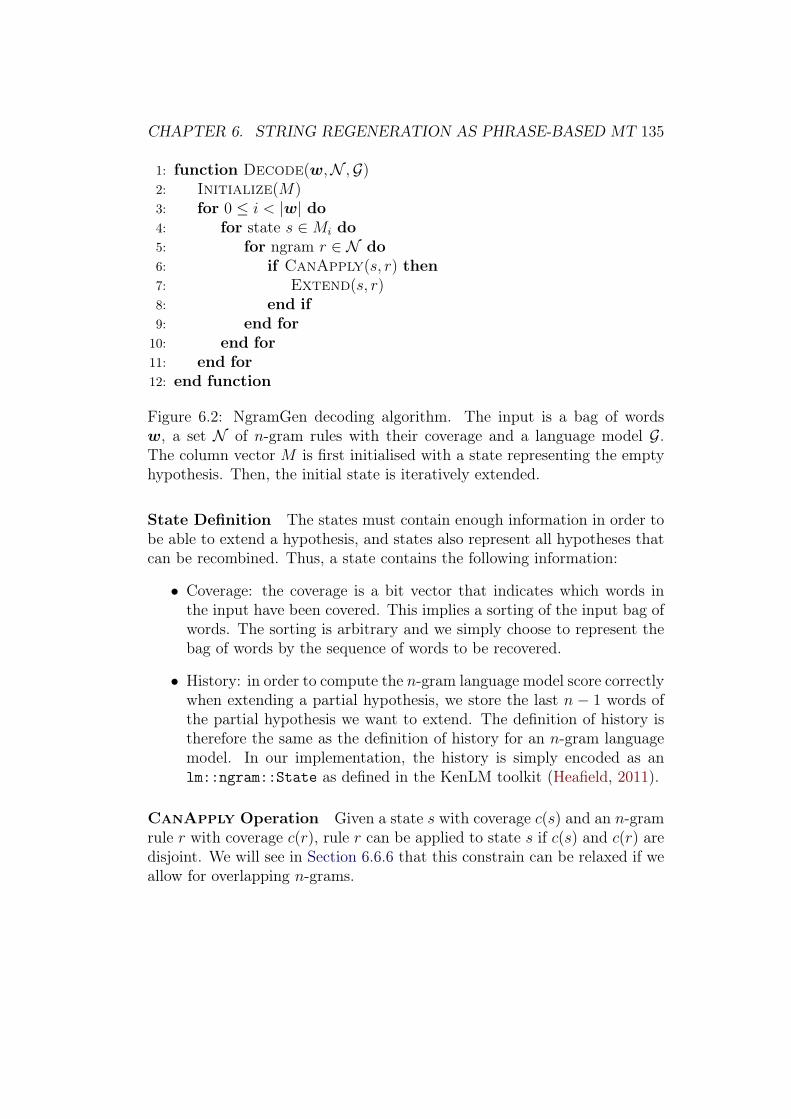
CHAPTER 6. STRING REGENERATION AS PHRASE-BASED MT 135
1: function Decode(w,N ,G)2: Initialize(M)3: for 0 ≤ i < |w| do4: for state s ∈Mi do5: for ngram r ∈ N do6: if CanApply(s, r) then7: Extend(s, r)8: end if9: end for
10: end for11: end for12: end function
Figure 6.2: NgramGen decoding algorithm. The input is a bag of wordsw, a set N of n-gram rules with their coverage and a language model G.The column vector M is first initialised with a state representing the emptyhypothesis. Then, the initial state is iteratively extended.
State Definition The states must contain enough information in order tobe able to extend a hypothesis, and states also represent all hypotheses thatcan be recombined. Thus, a state contains the following information:
• Coverage: the coverage is a bit vector that indicates which words inthe input have been covered. This implies a sorting of the input bag ofwords. The sorting is arbitrary and we simply choose to represent thebag of words by the sequence of words to be recovered.
• History: in order to compute the n-gram language model score correctlywhen extending a partial hypothesis, we store the last n − 1 words ofthe partial hypothesis we want to extend. The definition of history istherefore the same as the definition of history for an n-gram languagemodel. In our implementation, the history is simply encoded as anlm::ngram::State as defined in the KenLM toolkit (Heafield, 2011).
CanApply Operation Given a state s with coverage c(s) and an n-gramrule r with coverage c(r), rule r can be applied to state s if c(s) and c(r) aredisjoint. We will see in Section 6.6.6 that this constrain can be relaxed if weallow for overlapping n-grams.

CHAPTER 6. STRING REGENERATION AS PHRASE-BASED MT 136
Extend Operation Given a state s with coverage c(s) and and n-gramrule r with coverage c(r) that can be applied to s, we extend s with r into anew state s′ as follows:
• The coverage c(s′) of s′ is the bitwise OR of c(s) and c(r):
c(s′) = c(s) | c(r) (6.4)
• The new partial score sc(s′) for s′ is defined in terms of the partial scoresc(s) for s, the history h(s) and the rule r:
sc(s′) = sc(s) + λgg(r|h(s)) + λϕ ·ϕ(r) (6.5)
• If s′ already exists in the column corresponding to its coverage, thenthe score of the existing state is updated if sc(s′) is better than theexisting score. Otherwise, s′ is simply added as a new state to thecolumn corresponding to its coverage.
Pruning The search space for an input bag of size N is the number ofpermutations of the input, which is N ! if all input words are distinct. Wetherefore need to apply pruning during search to make the decoding processtractable. We support histogram pruning and threshold pruning (see Sec-tion 2.5.4). After each extension, if we add a new state, we enforce thatthe column where a state was added satisfies the pruning constraints. Thismeans that for histogram pruning, with m the maximum number of statesper column, if we add a new state to a column that has m states, then thestate with the lowest score is removed from that column.
For threshold pruning with a threshold t, the situation is slightly morecomplex. When we want to add a state s with score sc(s) to a column wherethe best score is b, we consider three cases:
• sc(s) ≤ b and sc(s) ≥ b− t: the state s is added to the column.
• sc(s) ≤ b and sc(s) < b− t: the state s is not added to the column.
• sc(s) > b: the state s is added to the column and all states in thatcolumn with a score less than sc(s)− t are removed from the column.
We have presented the decoding algorithm and various data structuresto support the algorithm. We will now describe how the set of hypotheses isencoded with FSTs.

CHAPTER 6. STRING REGENERATION AS PHRASE-BASED MT 137
6.5.3 FST Building
We mentioned in Section 6.5.2.2 that a state represents partial hypothesesthat can be recombined as well as the necessary information to be able toextend a partial hypothesis. However, since we do not keep backpointersbetween states, we cannot recover hypotheses directly from M , the vectorof columns. Instead, we build an FST that contains all hypotheses. Foreach extension, an arc is added to the output FST. We make use of theOpenFst toolkit (Allauzen et al., 2007). This allows us to rescore the outputusing tools already integrated with OpenFst (Blackwood, 2010). Anotheradvantage is that hypotheses that are recombined are not deleted and allcompleted hypotheses are stored in the output FST. This allows hypothesesthat would be discarded in recombination to remain in the output and getan opportunity to become the best hypothesis after rescoring.
6.5.4 Example
We now demonstrate how our algorithm works with an example. Our inputconsists of:
• a bag of words: [do, you, do]. Note that the word do is repeated.
• a bigram language model. Thus the history for each state will consistof the last word of the partial hypothesis.
• monolingual n-gram rules with their coverage of the input bag of words.We use the rules listed in Table 6.1.
After running our algorithm without pruning, we obtain the data structurerepresented in Figure 6.3. We can see that the same state {111, do} is reusedfor the two hypotheses do you do, you do do, because these hypotheses havethe same coverage and the same history. We also note that the hypothe-sis do you do is repeated. This is not an issue as we use an operation ofdeterminisation on the resulting FST.
We will now present various experiments that demonstrate the effective-ness of our decoder for the string regeneration task. We will also analysevarious capabilities of the decoder in order to understand which configura-tions lead to better results.

CHAPTER 6. STRING REGENERATION AS PHRASE-BASED MT 138
N-gram Coveragedo 100do 001you do 011you do 110do you 110do you 011
Table 6.1: Example of input monolingual n-gram rules with their coverage,corresponding to the example input [do, you, do]. The FST representing theset of hypotheses obtained with these rules is represented in Figure 6.3.
..000, </s>.
100, do
. 011, do.
110, you
.
111, you
. 111, do.
do
. you do.
do you
.
do you
.
you do
. do.
do
Figure 6.3: Example of output obtained from running the NgramGen decoderon the input [do, you, do] with the rules listed in Table 6.1. Double circledaccepting states represent completed hypotheses.

CHAPTER 6. STRING REGENERATION AS PHRASE-BASED MT 139
6.6 ExperimentsIn this section, we will present various string regeneration experiments. Wefirst present a baseline without restriction on the input length. Then, we showhow the input can be split into chunks of maximum length for more rapidexperimentation. We then study the effect of pruning, n-gram rule length,the use of overlap between rules, the benefits of future cost estimation andfinally the benefits of applying rescoring to our first pass decoder.
6.6.1 Experimental Setup
We run string regeneration experiments on various data sets. We use thefollowing data sets:
• MT08-nw: the first English reference for the newswire portion of theArabic-English translation task for the NIST Open Machine Transla-tion 2008 Evaluation.2
• MT09-nw: the first English reference for the newswire portion of theArabic-English translation task for the NIST Open Machine Transla-tion 2009 Evaluation.3.
• WSJ22: Section 22 from the Penn Treebank.
• WSJ23: Section 23 from the Penn Treebank.
The test sets are first tokenised and lowercased. Then, n-gram rules upto length 5 for each of the processed test sets are extracted from a largemonolingual text collection. For MT08-nw and MT09-nw, we use all availablemonolingual data for the NIST Open Machine Translation 2012 Evaluation.4This consists of approximately 10.6 billion words. For WSJ22 and WSJ23,we use all available monolingual data for the WMT13 evaluation, describedin Table 5.2. This consists of approximately 7.8 billion words. For MT08-nwand MT09-nw, we estimate a modified Kneser-Ney 4-gram language modelon approximately 1.3 billion words of English text, including the AFP andXinhua portions of the Gigaword corpus version 4 and the English side of
2 http://www.itl.nist.gov/iad/mig/tests/mt/20083 http://www.itl.nist.gov/iad/mig/tests/mt/20094 http://www.nist.gov/itl/iad/mig/openmt12.cfm

CHAPTER 6. STRING REGENERATION AS PHRASE-BASED MT 140
Test Set BLEUMT08-nw 42.32MT09-nw 37.29WSJ22 44.01WSJ23 45.48
Table 6.2: Baseline for the NgramGen Decoder on the various test sets usedthroughout experimentation. No limits are imposed on the input length, thuspruning setting are set so that decoding is feasible on the given hardware.Performance is measured with case insensitive BLEU.
various Arabic-English parallel corpora used in MT evaluations. For WSJ22and WSJ23, we estimate a modified Kneser-Ney 4-gram language model onall available monolingual data for the WMT13 evaluation.
6.6.2 Baseline
We first run a baseline on our various test sets with the NgramGen decoder.Because there are no constraints on the input length, some long sentencesneed more pruning for the decoder to complete the procedure. Therefore, weuse a length dependent histogram pruning of 11000
length(input) . For example, for aninput sentence of length 100, this means that we use a histogram pruning of110 for that particular sentence. Results are reported in Table 6.2.
We also compare the performance obtained by the NgramGen decoderwith previous work on the data set WSJ23 in Table 6.3. We can see that ourmethod, without using any additional information apart from the input bag-of-word, achieves state-of-the-art performance. All other methods keep basenoun phrases as a single unit and also use additional syntactic informationsuch as part-of-speech tags.
In the section to follow, we impose length restrictions on the input bagof words in order to allow more rapid experimentation.
6.6.3 Sentence Splitting
Running the NgramGen decoder without limiting the length of the input asin Section 6.6.2 can be time and memory consuming. For more rapid exper-imentation, we only reorder chunks of a limited size in the input. The input
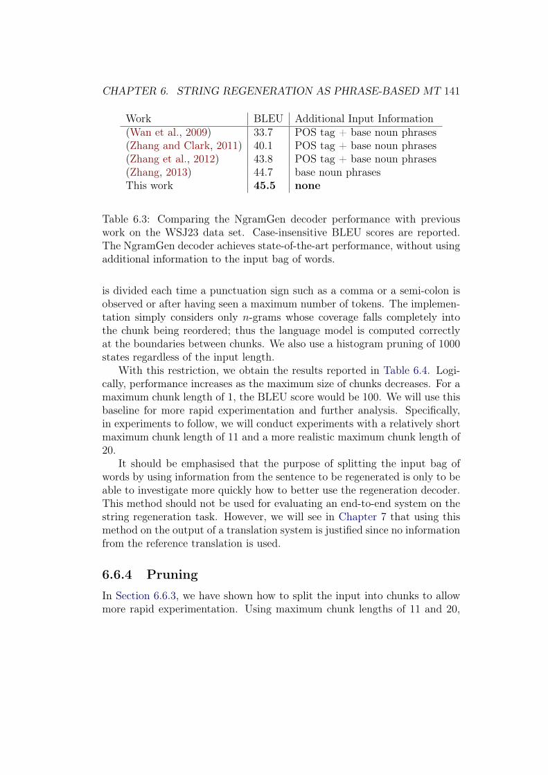
CHAPTER 6. STRING REGENERATION AS PHRASE-BASED MT 141
Work BLEU Additional Input Information(Wan et al., 2009) 33.7 POS tag + base noun phrases(Zhang and Clark, 2011) 40.1 POS tag + base noun phrases(Zhang et al., 2012) 43.8 POS tag + base noun phrases(Zhang, 2013) 44.7 base noun phrasesThis work 45.5 none
Table 6.3: Comparing the NgramGen decoder performance with previouswork on the WSJ23 data set. Case-insensitive BLEU scores are reported.The NgramGen decoder achieves state-of-the-art performance, without usingadditional information to the input bag of words.
is divided each time a punctuation sign such as a comma or a semi-colon isobserved or after having seen a maximum number of tokens. The implemen-tation simply considers only n-grams whose coverage falls completely intothe chunk being reordered; thus the language model is computed correctlyat the boundaries between chunks. We also use a histogram pruning of 1000states regardless of the input length.
With this restriction, we obtain the results reported in Table 6.4. Logi-cally, performance increases as the maximum size of chunks decreases. For amaximum chunk length of 1, the BLEU score would be 100. We will use thisbaseline for more rapid experimentation and further analysis. Specifically,in experiments to follow, we will conduct experiments with a relatively shortmaximum chunk length of 11 and a more realistic maximum chunk length of20.
It should be emphasised that the purpose of splitting the input bag ofwords by using information from the sentence to be regenerated is only to beable to investigate more quickly how to better use the regeneration decoder.This method should not be used for evaluating an end-to-end system on thestring regeneration task. However, we will see in Chapter 7 that using thismethod on the output of a translation system is justified since no informationfrom the reference translation is used.
6.6.4 Pruning
In Section 6.6.3, we have shown how to split the input into chunks to allowmore rapid experimentation. Using maximum chunk lengths of 11 and 20,

CHAPTER 6. STRING REGENERATION AS PHRASE-BASED MT 142
Maximum Chunk Length MT08-nw7 82.839 78.5311 74.8613 71.7515 68.9520 64.36
Table 6.4: NgramGen decoder baseline with restrictions on the input length.Case-insensitive BLEU scores are reported. For further experiments, maxi-mum chunk lengths of 11 and 20 will be used to contrast results on shorteror longer inputs. The BLEU score for a maximum chunk length of 1 wouldevidently be 100.
we will study the effect of various histogram pruning thresholds.Results are reported in Table 6.5. In both maximum input length set-
tings, performance increases as the maximum number of states per columnincreases. For a maximum input length of 11, performance improves by 0.39BLEU (0.5% relative, row 1 vs. row 7). For a maximum input length of 20,performance improves by 1.18 BLEU (1.8% relative, row 8 vs. row 14). Thisis due to a larger search space being explored in the case of a maximum inputlength of 20.
6.6.5 n-gram Order for n-gram Rules
As mentioned in Section 6.2, previous work complements the use of n-gramlanguage models with syntactic information for the string regeneration taskor for the tree linearisation task. In this work, n-gram language modelsare complemented by the use of n-gram rules extracted from large amountsof monolingual text. In this section, we observe the impact of using allrules from unigrams up to 5-grams or only using rules with specific lengths.Specifically, we compare the following configurations:
• All n-gram orders: this is the default used in experiments so far.
• Unigrams, 4-grams and 5-grams only: our motivation for this config-uration is to only use rules that are likely to produce a fluent output,

CHAPTER 6. STRING REGENERATION AS PHRASE-BASED MT 143
Row Histogram Pruning Max Input Length MT08-nw1 500 11 74.672 1000 11 74.863 1500 11 74.984 2000 11 75.025 3000 11 75.096 4000 11 75.087 5000 11 75.068 500 20 64.219 1000 20 64.3610 1500 20 64.8511 2000 20 64.9412 3000 20 65.1713 4000 20 65.3314 5000 20 65.39
Table 6.5: Effect of histogram pruning on performance with a maximuminput length of 11 and 20. Case-insensitive BLEU scores are reported. Inboth maximum input length settings, increasing the maximum column sizeincreases performance, but more so with maximum input length of 20 sincethe search space is much larger in that case.
CHAPTER 6. STRING REGENERATION AS PHRASE-BASED MT 144
namely 4-grams and 5-grams. We always use unigrams in order to ob-tain complete hypotheses. For example, if we only used 4-grams and5-grams, an input bag of words of size 6 could never be covered, unlessoverlapping rules were allowed (see Section 6.6.6).
• Unigrams and 5-grams only: our motivation is identical to using onlyunigrams, 4-grams and 5-grams.
• Unigrams only: in this setting, only the language model informs the de-coder. This setting is similar to the one mentioned in Section 6.2 whereall permutations are considered and ranked by the language model. Ourmotivation for this setting is to investigate whether n-gram rules areat all useful for string regeneration.
Results are reported in Table 6.6. We can see that for a relatively shortmaximum of 11 on the input length, using more n-gram orders is alwaysbeneficial. Because the maximum input length is short, the search space canbe explored more thoroughly and this benefits configurations that generatelarger search spaces. For a more realistic maximum input length of 20, resultsare more in line with our initial motivation for each configuration. Comparingrow 6 vs. row 5, we can observe that removing lower order n-grams is slightlybeneficial. The same trend is observed when comparing row 7 vs. row 5.Finally, for both maximum input length configurations of 11 and 20, it isalways beneficial to use n-gram rules with n > 1.
6.6.6 Overlapping n-gram Rules
In Section 6.5.2.2, we defined the CanApply operation by requiring thatthe state coverage and the coverage of the rule used to extend the state bedisjoint. In this section, we relax this constraint to allow for a coverageintersection of a certain maximum overlapping length. The idea of allowingoverlapping rules has been used previously in phrase-based translation forcreating phrase tables with longer rules (Tribble et al., 2003) but not indecoding.
Results are presented in Table 6.7. Configurations for overlapping rulesinclude no overlap, a maximum overlap of 1 or a maximum overlap of 2. Asin previous experiments, we contrast the effect of overlapping rules with amaximum input length of either 11 or 20. Decoding is run in parallel usingSun Grid Engine (Gentzsch, 2001). The total decoding time is measured as

CHAPTER 6. STRING REGENERATION AS PHRASE-BASED MT 145
Row Rule Configuration Max Input Length MT08-nw1 all rules 11 74.862 1g/4g/5g 11 74.853 1g/5g 11 74.824 1g only 11 74.135 all rules 20 64.366 1g/4g/5g 20 64.427 1g/5g 20 64.748 1g only 20 63.36
Table 6.6: Effect of selecting n-gram rules based on their n-gram order. Case-insensitive BLEU scores are reported. For a short maximum input length,using more orders is always beneficial because this increases a tractable searchspace. For a maximum input length of 20, retaining only n-gram rules withhigher order n-gram produces better results.
the sum of time spent on each job. We also study the effect of overlappingrules when all n-gram orders are included (rule configuration “all”) or whenonly unigrams and 5-grams are allowed (rule configuration “1g/5g”). Wehypothesise that overlapping rules may be more beneficial when lower n-gramorders are missing. However, we observe that that allowing for overlappingrules does not improve performance, apart from increasing the search spaceand decoding time in general. We do not use this decoder capability in futureexperiments.
6.6.7 Future Cost
The justification for adding a future cost estimate to the partial hypothesisscore is analogous to the one provided for phrase-based translation in Sec-tion 2.5.4. Hypotheses that cover the same number of words in the inputbag of words are grouped together in a stack and hypotheses with costs thatare too high are pruned out. However, these hypotheses may not be di-rectly comparable, because some hypotheses cover very frequent words thatare favoured by the language model while other hypotheses may cover infre-quent words. We therefore estimate a future cost for each hypothesis. Thisfuture cost is added to the partial hypothesis cost for pruning purposes.
We investigate the effect of using a unigram language model to estimate

CHAPTER 6. STRING REGENERATION AS PHRASE-BASED MT 146
Row Overlap Max Input Length Rule MT08-nw TotalConfiguration Time (s)
1 no overlap 11 all 74.86 200752 1 11 all 74.87 196853 2 11 all 74.85 182004 no overlap 11 1g/5g 74.82 67745 1 11 1g/5g 74.81 86266 2 11 1g/5g 74.80 88057 no overlap 20 all 64.36 572858 1 20 all 64.39 899899 2 20 all 64.28 9577510 no overlap 20 1g/5g 64.74 1342011 1 20 1g/5g 64.72 2031412 2 20 1g/5g 64.63 22522
Table 6.7: Effect of allowing for overlapping rules. Case-insensitive BLEUscores are reported. In all configurations, allowing for overlapping rules doesnot improve performance. In addition, overlapping rules increase decodingtime in general.

CHAPTER 6. STRING REGENERATION AS PHRASE-BASED MT 147
Configuration Max Input Length MT08-nwno future cost estimate 11 74.86future cost estimate 11 75.10no future cost estimate 20 64.36future cost estimate 20 65.05
Table 6.8: Effect of using a future cost estimate for pruning. Case-insensitiveBLEU scores are reported. Future cost is computed with a unigram languagemodel. Future cost is beneficial for both a relatively short maximum inputlength of 11 and for a more realistic maximum input length of 20, withrespective improvements of 0.24 BLEU and 0.69 BLEU.
the future cost. Given a partial hypothesis, its future cost is defined by theunigram language model score of the words from the input bag of words thatare not covered by the partial hypothesis. Because there is no notion of wordordering in the input, we cannot easily use a higher order n-gram languagemodel language model to estimate future cost.
We compare the use of future cost estimates with maximum input lengthsof 11 and 20, as in previous experimentation. Results are reported in Ta-ble 6.8. In both settings, adding a unigram language model as future costestimate to the cost of a partial hypothesis for pruning is beneficial. For ashort maximum length of 11 on the input length, we obtain a gain of 0.24BLEU while for a maximum input length of 20, we obtain a gain of 0.69BLEU.
6.6.8 Rescoring
In Section 6.5.3, we described how the NgramGen decoder generates an FSTthat encodes a set of hypotheses. We choose this output format in orderto be able to apply various lattice rescoring techniques that also utilise thisformat as input (see Section 2.10.1, Section 2.10.2 and Section 2.10.3).
In this section, we show that these rescoring techniques are not onlyeffective on the output of a first pass translation decoder but also in ourstring regeneration setting. Specifically, we run 5-gram language model lat-tice rescoring as well as LMBR lattice rescoring experiments. LMBR appliedto hypothesis combination, described in Section 2.10.2, will be applied inChapter 7.

CHAPTER 6. STRING REGENERATION AS PHRASE-BASED MT 148
Configuration MT08-nw MT09-nw WSJ22 WSJ23first pass 64.36 60.91 62.76 64.39+5g 66.11 63.26 63.18 65.04+LMBR 67.37 64.53 64.28 65.85
Table 6.9: Effect of lattice rescoring on the first pass lattices obtained by theNgramGen decoder. Case-insensitive BLEU scores are reported. Rows “+5g”and “+LMBR” show large BLEU gains with respect to first pass decoding,demonstrating the effectiveness of these lattice rescoring techniques acrossvarious tasks, including translation and string regeneration.
Results are reported in Table 6.9, on all our test sets. The MT08-nw setis used to tune LMBR parameters, and these parameters are tested on theMT09-nw set. Similarly, WSJ22 is used as a tuning set for WSJ23. Becausewe only use a single language model as the only feature and because in alldecoder hypotheses, the length is identical, there is no tuning or testing setfor first-pass decoding or 5-gram language mode rescoring.
We can see that large BLEU gains are obtained in 5-gram rescoring:+1.29 BLEU on average across all test sets. LMBR rescoring also providesan average gain of 2.54 BLEU with respect to first pass decoding over thetest sets MT09-nw and WSJ23.
6.7 ConclusionIn this chapter, we have presented a novel approach to the string regenerationtask, inspired from phrase-based models for SMT. We have implementeda decoder, NgramGen, that operates in a similar fashion to phrase-basedstack-based decoders and achieves state-of-the-art performance on the stringregeneration task from a simple bag of words on the Penn Treebank Section23 data set.
We have also analysed various capabilities of our decoder. From thisanalysis, we draw the following conclusions:
• Removing lower order n-gram rules other than unigrams, which areneeded to ensure that the input can be covered entirely, improves per-formance.

CHAPTER 6. STRING REGENERATION AS PHRASE-BASED MT 149
• Allowing for overlapping rules slows down the decoding procedure anddoes not provide gains in our experiments.
• Future cost estimates improve the pruning procedure and overall per-formance.
• Lattice rescoring techniques are applicable and provide gains in thestring regeneration setting.
In the following chapter, we will explore potential application of our de-coder to word reordering in machine translation. We will consider the outputof a machine translation decoder as the input bag of words for the regenera-tion decoder.

Chapter 7
String Regeneration Applied toMachine Translation
In Chapter 6, we have introduced techniques for string regeneration inspiredfrom the phrase-based translation paradigm. We have demonstrated theireffectiveness and achieved state-of-the-art performance in terms of BLEU onthe string regeneration task on the Penn Treebank. In this chapter, we willattempt to apply these techniques to the output of a machine translationsystem. One key difference is that the quality of the input bag of words issubstantially lower when regenerating translation output instead of regener-ating an original English sentence.
Our motivation is the general motivation for the rescoring paradigm. In-stead of allowing any kind of reordering in first pass decoding, which wouldmake the search space intractable, we first create a search space of relativelyhigh quality, then we relax reordering constraints. We will show that us-ing our string regeneration decoder, we are able to match the quality of ourtranslation system. In some instances, we show very slight gains in perfor-mance. This work is meant to lay the ground work for future incorporationof natural language generation into SMT.
In Section 7.1, we describe our machine translation baseline system. InSection 7.2, we describe our string regeneration baseline, both with and with-out future cost estimates. Because the regeneration baseline degrades perfor-mance with respect to the translation baseline, we carry out an error analysisin Section 7.3. In Section 7.4 and in Section 7.5, we show two ways of in-corporating information from the translation system in order to match thetranslation system quality; in some instances, we obtain very slight improve-
150

CHAPTER 7. STRING REGENERATION FOR TRANSLATION 151
ments over the MT baseline.
7.1 SMT Baseline SystemIn this section, we briefly summarise the machine translation system usedas a baseline for our string regeneration rescoring experiments. The Cam-bridge University Engineering Department participated in the NIST 2012translation competition.1 We describe here the Chinese-English system. Wepick this language pair rather than for example Arabic-English simply be-cause Chinese and English are quite distant in terms of word ordering (seeSection 2.6.1).
We use all the Chinese-English parallel data available for the constrainedtrack. Parallel data consists of 9.2M sentence pairs, 203M tokens on the Chi-nese side and 218M tokens on the English side, after preprocessing. Paralleldata is aligned using a word-to-phrase HMM model with the MTTK toolkit(see Section 2.3.1). In the source-to-target direction, the maximum size ofa Chinese phrase is 2 while in the target-to-source direction, the maximumsize of an English phrase is 4. The final alignments are obtained by takingthe union of Viterbi alignments obtained in both source-to-target and target-to-source directions. A hierarchical phrase-based grammar is then extractedfrom the alignments using the infrastructure described in Section 3.4.
We build a first-pass language model using the target side of the paral-lel text and the AFP and Xinhua agencies of the Gigaword corpus (Parkeret al., 2009). We first build separate modified Kneser-Ney smoothed 4-gramlanguage models (see Section 2.7.3) on each of these three corpora. The lan-guage models built on AFP and Xinhua are interpolated with equal weights.The resulting language model is interpolated with the language model builton the target side of the parallel text with equal weights. We also build asecond-pass Stupid Backoff 5-gram language model for rescoring as describedin Section 2.10. The output of 5-gram rescoring is rescored with LMBR (seeSection 2.10.2).
We use the features described in Section 2.6.5 as well as 36 provenancerelated features (see Section 5.5). The union strategy is employed for testset grammar filtering, as described in Section 5.5. In this chapter, all resultsare reported on an internal tuning set (Tune) in the newswire domain com-
1 http://www.nist.gov/itl/iad/mig/openmt12.cfm
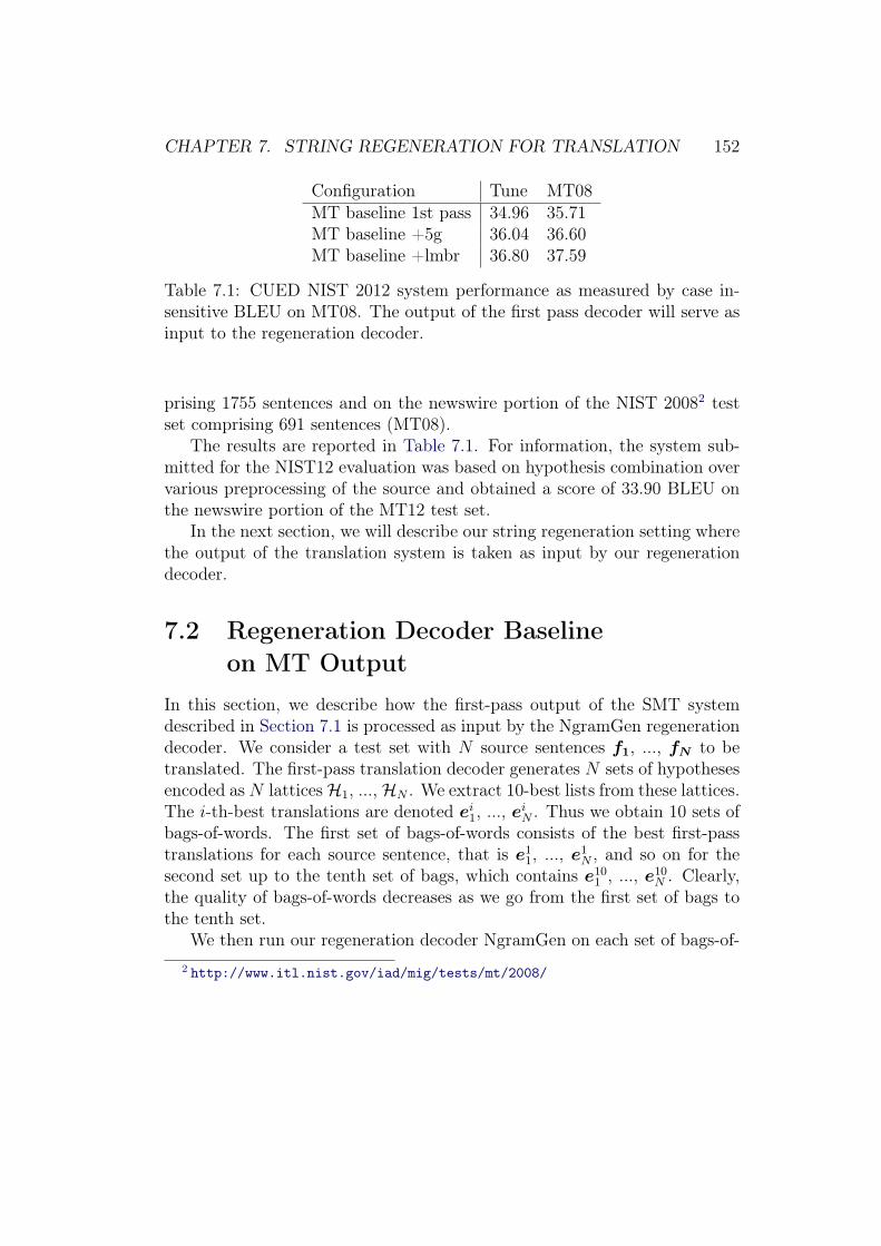
CHAPTER 7. STRING REGENERATION FOR TRANSLATION 152
Configuration Tune MT08MT baseline 1st pass 34.96 35.71MT baseline +5g 36.04 36.60MT baseline +lmbr 36.80 37.59
Table 7.1: CUED NIST 2012 system performance as measured by case in-sensitive BLEU on MT08. The output of the first pass decoder will serve asinput to the regeneration decoder.
prising 1755 sentences and on the newswire portion of the NIST 20082 testset comprising 691 sentences (MT08).
The results are reported in Table 7.1. For information, the system sub-mitted for the NIST12 evaluation was based on hypothesis combination overvarious preprocessing of the source and obtained a score of 33.90 BLEU onthe newswire portion of the MT12 test set.
In the next section, we will describe our string regeneration setting wherethe output of the translation system is taken as input by our regenerationdecoder.
7.2 Regeneration Decoder Baselineon MT Output
In this section, we describe how the first-pass output of the SMT systemdescribed in Section 7.1 is processed as input by the NgramGen regenerationdecoder. We consider a test set with N source sentences f1, ..., fN to betranslated. The first-pass translation decoder generates N sets of hypothesesencoded as N latticesH1, ...,HN . We extract 10-best lists from these lattices.The i-th-best translations are denoted ei
1, ..., eiN . Thus we obtain 10 sets of
bags-of-words. The first set of bags-of-words consists of the best first-passtranslations for each source sentence, that is e1
1, ..., e1N , and so on for the
second set up to the tenth set of bags, which contains e101 , ..., e10
N . Clearly,the quality of bags-of-words decreases as we go from the first set of bags tothe tenth set.
We then run our regeneration decoder NgramGen on each set of bags-of-2 http://www.itl.nist.gov/iad/mig/tests/mt/2008/

CHAPTER 7. STRING REGENERATION FOR TRANSLATION 153
words separately. The configuration for running the decoder on the i-th setof bags is called ith-best. We obtain N lattices L1
1, ..., L1N for the first set
of bags, and so on for the second set of bags to the tenth set of bags, forwhich we obtain N lattices L10
1 , ..., L10N . Performance is measured on each
separate set of NgramGen output lattices. Intuitively, we can predict thatthe performance will decrease from the NgramGen output for the first set ofbags to the NgramGen output for the tenth set of bags.
We also form the union of lattices obtained from each set: for the i-th source sentence fi, we form the union of the lattices L1
i , ..., L10i . This
configuration is simply called union. We use the following settings for theregeneration decoder:
• We use a histogram pruning of 1000, that is a maximum number of1000 states per column (see Section 6.5.2.2).
• We split the input according to punctuation (comma and semi-colon),with a maximum chunk length of 11, as described in Section 6.6.3. Notethat contrary to the string regeneration settings, the splitting informa-tion comes from an MT hypothesis and not a reference. Therefore, itis legitimate to use input splitting for experimentation, decoding timesbecome more reasonable and the NgramGen hypotheses are constrainedto be close to the MT hypotheses, which we know have a relatively highquality already.
• As in Section 6.6.7, future cost is estimated with a unigram languagemodel.
Results are summarised in Table 7.2. The main observation is that for allregeneration configurations, there is a substantial drop in performance withrespect to the machine translation baseline. This is not unexpected sincewe are only using the language model feature for regeneration: except forthe bag-of-words obtained from the translation hypothesis and the splittingpoints for more efficient decoding, all information coming from the translationsystem is discarded.
We measured the performance of the oracle hypothesis for the translationsystem and the regeneration systems on the Tune set. Again, regenerationoracle BLEU scores are substantially lower than the translation oracle BLEU.However, it is interesting to observe that the oracle hypothesis obtained fromthe union configuration is around 9 BLEU points above the MT baseline.

CHAPTER 7. STRING REGENERATION FOR TRANSLATION 154
This indicates that there is a possible reordering of the 10-best hypothesesobtained by the translation decoder that improves translation quality.
Experiments were run with and without future cost estimates. We obtainsmall gains when future cost estimates are used (see column 3 vs. column1,column vs. column 2 and column 6 vs. column 5) but gains are very smallcompared to what was obtained when regenerating a well-formed Englishsentence as in Section 6.6.7.
Finally, as predicted, because the quality of the bags decreases from the1st-best configuration to the 10th-best configuration, performance after re-generation from these sets of bags also decreases. In the next section, wewill analyse the drop in performance for the regeneration configuration withrespect to the MT baseline.
7.3 Analysis of the Loss of MT HypothesesWe have observed in the previous section that simply reordering the n-bestoutput of the translation decoder with our regeneration decoder gives a dropin performance with respect to the performance obtained by the baselinetranslation system. Although the translation system output lacks fluencydue to word reordering problems, we know that the quality of this outputis relatively high, thus we would like the output of the regeneration step tostay relatively close to the MT hypothesis. In this section, we will examinehow often the MT hypothesis is not regenerated at all in the regenerationlattices, how often it is chosen as a regeneration hypothesis and at whatpoint in the decoding procedure the MT hypothesis disappears from theregeneration lattice. We carry out this analysis on the 1st-best configurationfrom Table 7.2 and on the Tune set.
The MT hypothesis is present in the regeneration lattice 92.3% of thetime when no future cost is estimated and 95.3% of the time with future costestimates. This is somewhat reassuring because these numbers imply thatthe language model score of the MT hypothesis is high enough so that theMT hypothesis is not very frequently discarded by pruning in regeneration.In contrast, the MT hypothesis is chosen as the best hypothesis by the regen-eration decoder only 43.6% of the time, with or without future costs. Thismeans that, most of the time, the MT hypothesis is present in the regen-eration lattice, but not chosen as the best regeneration hypothesis, simplybecause its model score, computed by the language model only, is lower than

CHAPTER 7. STRING REGENERATION FOR TRANSLATION 155
Column 1 2 3 4 5 6Set Tune Tune Tune Tune MT08 MT08Oracle ! !
MT baseline 1st pass 34.96 56.12 34.96 56.12 35.71 35.71Future Cost ! ! !
1st-best 33.37 39.14 33.40 39.18 32.78 32.792nd-best 33.16 38.93 33.22 39.02 32.77 32.773rd-best 33.14 38.84 33.17 38.91 32.54 32.554th-best 33.13 38.80 33.16 38.87 32.35 32.395th-best 33.20 38.95 33.28 39.00 32.12 32.176th-best 33.08 38.74 33.12 38.81 32.33 32.407th-best 33.19 39.00 33.24 39.05 32.16 32.188th-best 32.98 38.79 33.04 38.84 32.11 32.149th-best 32.71 38.59 32.75 38.65 32.11 32.1110th-best 33.05 38.81 33.11 38.88 32.50 32.55union 32.85 43.96 32.90 44.00 32.11 32.18
Table 7.2: Regeneration experiments on input bags obtained from the 10-best hypotheses of a translation system. Case-insensitive BLEU scores arereported. 10-best lists are generated by an MT system. Each set of nth-best hypotheses is used as a set of input bags-of-words for the NgramGendecoder. Oracle performance on the Tune set is also measured. Regenerationdecoding experiments are repeated with and without future cost estimates.Substantial drops in performance are observed in regeneration with respectto the translation baseline. Oracle scores for the union configuration showthat by simply improving word reordering on the 10-best output of the MTsystem, gains may be achieved. Future cost estimates provide very smallgains.

CHAPTER 7. STRING REGENERATION FOR TRANSLATION 156
0
5
10
15
20
25
30
0-10 10-20 20-30 30-40 40-50 50-60 60-70 70-80 80-90 90-100
Pro
port
ion
of lo
st M
T h
ypot
hese
s (%
)
Proportion of words covered (%)
Lost MT hypotheses vs. words covered
Figure 7.1: Analysis of when the MT hypothesis is lost. The x-axis representsbins of 10% for the relative size of the input bag-of-word. The y-axis is simplythe count of instances.
the score of another regeneration hypothesis.For the case when the MT hypothesis is not present in the regeneration
lattice, we further analyse at which point the MT hypothesis is lost duringthe decoding procedure. As described in Section 6.5.2.2, a state is definedby coverage and history. For this analysis, we add a Boolean variable to thestate definition that indicates whether the partial input is one of the partialhypotheses represented by this state. We can then easily compute after howmany words covered the MT hypothesis has been lost.
Figure 7.1 illustrates the proportion of MT hypotheses lost vs. the pro-portion of input words covered. The plot shows that MT hypotheses can belost quite early in the process, as early as when 20% of the size of the inputbag-of-word has been covered. Using future cost estimates produces a verysimilar graph and does not alleviate the problem of losing MT hypothesesearly in the decoding process.
From this analysis, we conclude that using the language model score asa single feature is not adequate for the task of regeneration from translationoutput. Designing and implementing additional features is a worthwhile op-portunity for future work. In the sections to follow, while keeping a single

CHAPTER 7. STRING REGENERATION FOR TRANSLATION 157
feature for regeneration, we will study alternative ways to bring the regener-ation output closer to the translation output.
7.4 Biased Language Model for RegenerationWe have shown in Section 7.3 that the MT hypothesis, which is known to be ofrelatively high quality, is not chosen as the best regeneration hypothesis morethan half of the time and is sometimes not even present in the regenerationlattice. In this section, we describe a first solution to remedy this issue andbring the regeneration output closer to the translation output.
Our solution is simply to bias the language model towards the MT hypoth-esis. In order to do this, we first compute n-gram posterior probabilities fromthe 1st-pass translation lattices (see Section 2.10.2). These posteriors arethen converted to integer counts in order to estimate a Good-Turing (Good,1953; Chen and Goodman, 1998) smoothed 4-gram language model fromthese counts. We then interpolate this language model with the originallanguage model with various interpolation parameters.
We report on experiments that are carried out on the set of bags obtainedfrom the best MT hypotheses; experiments on lower quality bags gave anal-ogous results. Interpolation parameters range from 0.4 (weight assigned tothe original language model) to 0.99. We obtain the results in Table 7.3. Wecan see that we are able to obtain hypotheses that have the same quality asthe MT hypotheses, and for an interpolation weight of 0.7, we obtain a veryslight improvement on the tuning set. We also obtain very similar resultswhen future cost estimates are included.
We use the best configuration from Table 7.3 (interpolation weight of 0.7)to run our regeneration decoder on the test set MT08 and obtain the resultsin Table 7.4. We obtain slight gains in terms of BLEU score on the MT08test using this technique.
7.5 Translation and RegenerationHypothesis Combination
In Section 7.4, we have described a first solution to bringing the qualityof regeneration to the level of translation: biasing the language model us-ing MT posteriors. Another possibility is exploit the system combination

CHAPTER 7. STRING REGENERATION FOR TRANSLATION 158
Configuration TuneMT baseline 1st pass 34.96Future Cost !
1st-best 33.37 33.401st-best 0.4 34.96 34.951st-best 0.5 34.96 34.961st-best 0.6 34.96 34.961st-best 0.7 34.97 34.961st-best 0.8 34.94 34.941st-best 0.9 34.90 34.901st-best 0.95 34.81 34.811st-best 0.99 34.11 34.13
Table 7.3: Regeneration experiments on the set of bags obtained from thebest MT hypotheses, with biased language models. Case-insensitive BLEUscores are reported. The original language model is interpolated with a lan-guage model built from MT posteriors. A range of interpolation parametersis experimented on. It is possible to recover the MT performance whenthe interpolation weight for the MT posterior based language model is largeenough. Including future cost estimates gives very similar results.
Configuration Tune MT08MT baseline 1st pass 34.96 35.711st-best 0.7 34.97 35.751st-best 0.7 future cost 34.96 35.75
Table 7.4: Regeneration with a language model biased towards MT posteri-ors. Case-insensitive BLEU scores are reported. The best configuration fromTable 7.3 is used to carry out regeneration on the MT08 test set. Very slightgains are observed.

CHAPTER 7. STRING REGENERATION FOR TRANSLATION 159
Configuration Tune MT08MT baseline +lmbr 36.80 37.59NgramGen 1-best baseline 36.81 37.29NgramGen union baseline 36.81 37.50NgramGen 1-best baseline future cost 36.82 37.45NgramGen union baseline future cost 36.81 37.50NgramGen 1-best interpolation 0.7 36.82 37.39NgramGen union interpolation 0.7 36.78 37.59NgramGen 1-best interpolation 0.7 Future Cost 36.81 37.39NgramGen union interpolation 0.7 Future Cost 36.77 37.60
Table 7.5: Experiments in hypothesis combination between the 5-gramrescored output of the translation decoder and the 5-gram output of theregeneration decoder.
paradigm. Because the regeneration decoder produces FSTs, we can reusean existing hypothesis combination system based on FSTs and described inSection 2.10.3. Hypothesis combination can also be used in conjunction withthe biased language model presented in Section 7.4.
The output of the regeneration decoder is first rescored with the large5-gram language model described in Section 7.1 and then combined with the5-gram rescored MT hypotheses. We experiment on the 1-best configuration(the set of bags is obtained from the best first-pass MT hypotheses) and onthe union configuration (see Section 7.2). Configurations for the regenerationdecoder also include the baseline reported in Section 7.2 as well as the biasedlanguage model method with an interpolation weight of 0.7 presented inSection 7.4.
Results are reported in Table 7.5. We can observe that using the unionof lattices produced by NgramGen is beneficial for hypothesis combination:more hypotheses are present in lattices obtained with the union configura-tion. Using the biased language model described in the previous section, weare able to match and obtain a very slight gain over the LMBR rescoredtranslation hypotheses.

CHAPTER 7. STRING REGENERATION FOR TRANSLATION 160
7.6 ConclusionIn this chapter, we have demonstrated how to apply our regeneration decoderto the output of a translation system in a 10-best hypothesis rescoring set-ting. Because the regeneration decoder only uses a language model as singlefeature and throws away word order information obtained from the transla-tion system except for splitting the input bag of words, by simply applyingthe NgramGen decoder to the output of the translation system, translationperformance is degraded.
We have shown two possible ways of integrating the information fromthe translation system into the regeneration system in order to match andslightly outperform the translation quality obtained by the translation sys-tem. The first solution is to bias the language model used in regenerationtowards the MT hypotheses by building an interpolated model between theoriginal language model and a language model built on the MT posteriors.The second solution simply takes advantage of the hypothesis combinationparadigm. In addition, both solutions were used in conjunction by combin-ing the output of the MT system with the output of the regeneration systemwhere the language model was biased.
One possible avenue for future work is to design and implement additionalfeatures in the decoder. The use of a few simple features, such as word andrule count, was already investigated but these features were not found to bebeneficial. Because the regeneration system was introduced into translationwith no loss in performance, another interesting next goal will be to keepidentical performance and use the NgramGen system in order to improvefluency.

Chapter 8
Summary and Future Work
Statistical Machine Translation was originally framed as a source-channelmodel with two main components, the translation model and the languagemodel. This separation into two modules provided opportunities for improv-ing each module individually, with the hope that improving the languagemodel would improve fluency while improving the translation model wouldimprove adequacy. Current state-of-the-art SMT systems include many morecomponents that interact in complex ways but also provide further individualimprovement opportunities.
In this thesis, we present various improvements and analyses in the SMTpipeline, with an emphasis on refining hierarchical phrase-based models. InSection 8.1, we review the contributions of this thesis and in Section 8.2, wepropose possible future work for each our contributions.
8.1 Review of WorkThis thesis demonstrated various refinements in hierarchical phrase-basedtranslation systems. A scalable infrastructure was developed for generat-ing and retrieving rules from hierarchical grammars. We also developed anoriginal training method for hierarchical phrase-based models which lever-ages computationally efficient HMM models usually used for word alignment.Other SMT pipeline components were refined: we studied the effect of ad-ditional grammar features for domain adaptation and provided recommen-dations for language models to be used in first-pass decoding and rescoring.Finally, we developed a string regeneration system from the ground up, anal-
161

CHAPTER 8. SUMMARY AND FUTURE WORK 162
ysed its competitive performance in the string regeneration task and its po-tential application to rescoring machine translation output. We now revieweach of these contributions.
8.1.1 Hierarchical Phrase-Based Grammars: Infrastruc-ture
In order to enable more rapid experimentation and to ensure scalability forhierarchical phrase-based grammar extraction and retrieval, we developed aflexible MapReduce implementation of the grammar extraction and estima-tion algorithm (Dyer et al., 2008). Our implementation described in Chap-ter 3 includes extensions for the computation of provenance features (Chianget al., 2011) and arbitrary corpus-level features can be added very easily toour framework.
A framework relying on the HFile format for efficient retrieval of hierarchi-cal rules to be used in test set decoding was also developed. Comprehensivetime and memory measurements demonstrated that our system is competi-tive with respect to linearly scanning, possibly concurrently, the datastruc-ture containing the grammar extracted from parallel text (Pino et al., 2012).
8.1.2 Hierarchical Phrase-Based Grammars: Modelling
In the SMT pipeline, the word alignment module and the grammar extrac-tion and estimation module usually interact through a fixed set of alignmentlinks produced by the word alignment models. Our contribution was to al-low for more communication between these two modules (de Gispert et al.,2010b). In Chapter 4, we first reframed the rule extraction procedure into ageneral framework. Under this framework, we introduced two novel methodsfor grammar extraction and estimation based on word alignment posteriorprobabilities.
The link posterior extraction method was based on alignment link poste-rior probabilities and allowed to extract a greater number of rules more reli-ably. The phrase pair posterior method was based on phrase pair alignmentposterior probabilities and was shown to provide a better estimated transla-tion model. Both methods provided substantial gains in translation qualityin a medium size Chinese-English translation task. Alternative strategies forcombining source-to-target and target-to-source word alignment models were

CHAPTER 8. SUMMARY AND FUTURE WORK 163
also investigated; hypothesis combination obtained the best performance inour experiments.
8.1.3 Hierarchical Phrase-Based System Development
The translation model, refined in Chapter 4, is one of the main features inthe log-linear model for translation. In Chapter 5, we studied the effect ofprovenance features (Chiang et al., 2011) for domain adaptation. The con-cept of provenance feature was extended from provenance lexical translationfeatures to provenance translation features. We demonstrated that, whenrule filtering thresholds are applied for each provenance and all survivingrules are kept, translation gains can be obtained.
We also provided recommendations for language modelling both in first-pass translation and rescoring. In the context of domain adaptation, we foundthat the best strategy for language modelling was off-line linear interpolationof various language models with weights tuned for perplexity on a held-outdevelopment set as opposed to log-linear interpolation with weights tunedby MERT. We also observed that when a few billion words of monolingualdata were available, a two-pass strategy of first-pass decoding with a 4-gramlanguage model trained on all data followed by 5-gram rescoring provided thebest performance in our experiments. Finally we confirmed in the rescoringsetting previous observations (Brants et al., 2007) in the first-pass decodingsetting that Kneser-Ney smoothing produced better translation quality thanStupid Backoff smoothing. Thus we obtained translation quality gains overthe top ranking system in the WMT13 Russian-English task (Pino et al.,2013).
8.1.4 Fluency in Hierarchical Phrase-Based Systems
One main reason for the lack of fluency in machine translation output isa discrepancy in word order between distant language pairs such as Chi-nese and English. In Chapter 6, we studied the problem of word orderingin isolation through the string regeneration task. We described a regenera-tion model inspired from the phrase-based translation model. We also builta regeneration decoder analogous to a stack-based decoder for translation.We achieved state-of-the-art performance on the string regeneration task.Finally, we analysed various capabilities of the decoder.

CHAPTER 8. SUMMARY AND FUTURE WORK 164
In Chapter 7, we applied string regeneration to the output of a translationsystem in a 10-best rescoring setting. Performance was degraded, however,by combining information obtained from the translation system with theregeneration system, we were able to match the quality of the translationoutput.
8.2 Future WorkThe retrieval framework presented in Chapter 3 can exploit parallelisationin two ways for further speed improvements. First, source pattern instancescan be generated for each test set source sentence individually; then eachsource sentence can processed in parallel. Because the HFile format doesnot allow multithreaded reads, one way to implement this solution is toreuse the multiprocessing capability of the MapReduce framework. Anotheropportunity for parallelisation similar to the one just described is to processqueries in parallel. Again, care has to be taken to use a multiprocessingapproach rather than a multithreading approach. Finally, the source patterninstance creation step can be fine-tuned in order to approach the speed of areal time system at the sentence level.
In Chapter 4, the rule extraction algorithm was described in a frame-work involving source constraints, alignment constraints, target constraints,a ranking function and a counting function. This provides an opportunityfor future work by investigating alternatives to the definitions of these con-straints and ranking and counting functions. Specifically, other word align-ment models may be explored.
In Chapter 5, we recommended to use a two-pass decoding strategy andwe also concluded that Kneser-Ney smoothing was beneficial over StupidBackoff smoothing in 5-gram language model rescoring. These recommenda-tions are valid for language models built on a few billion words. In the future,we will revise them with language models trained on an order of magnitudemore monolingual data.
We successfully applied phrase-based models and decoding techniques tothe task of string regeneration in Chapter 6. However, interesting futurework may be carried out to investigate the effect of using more features thansimply a language model. In addition, we may study how overlapping rulescan be used to obtain more chances of covering the entire input if no unigramrules are used.

CHAPTER 8. SUMMARY AND FUTURE WORK 165
The effect of additional features for the regeneration decoder may alsobe studied in the regeneration of translation output setting. If translationquality as measured BLEU does not increase, efforts will be dedicated toimprove fluency while maintaining translation quality. Finally, more sophis-ticated future cost estimates may be studied, such as n-gram language modelwith n > 1: this is possible because when regenerating translation output,the word ordering information is legitimately available in the input.

Bibliography
Alfred V. Aho and Jeffrey D. Ullman. Syntax directed translations and thepushdown assembler. Journal of Computer and System Sciences, 3(1):37–56, 1969. 28
Cyril Allauzen, Mehryar Mohri, and Brian Roark. Generalized Algorithmsfor Constructing Statistical Language Models. In Proceedings of the 41stMeeting of the Association for Computational Linguistics, pages 557–564,2003. 43
Cyril Allauzen, Michael Riley, Johan Schalkwyk, Wojciech Skut, andMehryar Mohri. OpenFst: A General and Efficient Weighted Finite-StateTransducer Library. In Proceedings of CIAA, pages 11–23, 2007. 137
Satanjeev Banerjee and Alon Lavie. METEOR: An Automatic Metric forMT Evaluation with Improved Correlation with Human Judgments. InProceedings of the ACL Workshop on Intrinsic and Extrinsic EvaluationMeasures for Machine Translation and/or Summarization, pages 65–72,Ann Arbor, Michigan, June 2005. Association for Computational Linguis-tics. URL http://www.aclweb.org/anthology/W/W05/W05-0909. 41, 126
Anja Belz, Bernd Bohnet, Simon Mille, Leo Wanner, and Michael White. Thesurface realisation task: Recent developments and future plans. In INLG2012 Proceedings of the Seventh International Natural Language Gener-ation Conference, pages 136–140, Utica, IL, May 2012. Association forComputational Linguistics. URL http://www.aclweb.org/anthology/W12-1525. 129
Oliver Bender, Evgeny Matusov, Stefan Hahn, Sasa Hasan, ShahramKhadivi, and Hermann Ney. The RWTH Arabic-to-English Spoken Lan-
166

BIBLIOGRAPHY 167
guage Translation System. In Proceedings of ASRU, pages 396–401, 2007.36
Adam L. Berger, Stephen A. Della Pietra, and Vincent J. Della Pietra. AMaximum Entropy Approach to Natural Language Processing. Computa-tional linguistics, 22(1):39–71, 1996. 10, 19, 20
Alexandra Birch, Chris Callison-Burch, Miles Osborne, and Philipp Koehn.Constraining the phrase-based, joint probability statistical translationmodel. In Proceedings on the Workshop on Statistical Machine Translation,pages 154–157, New York City, June 2006. Association for ComputationalLinguistics. URL http://www.aclweb.org/anthology/W/W06/W06-3123.76
Christopher M. Bishop. Pattern Recognition and Machine Learning.Springer-Verlag New York, Inc., Secaucus, NJ, USA, 2006. ISBN0387310738. 44
Graeme Blackwood. Lattice Rescoring Methods for Statistical Machine Trans-lation. PhD thesis, University of Cambridge, 2010. 45, 46, 137
Graeme Blackwood, Adria de Gispert, and William Byrne. Efficient PathCounting Transducers for Minimum Bayes-Risk Decoding of StatisticalMachine Translation Lattices. In Proceedings of the ACL 2010 ConferenceShort Papers, pages 27–32, Uppsala, Sweden, July 2010. Association forComputational Linguistics. URL http://www.aclweb.org/anthology/P10-2006. 45
Burton H. Bloom. Space/time trade-offs in hash coding with allowable errors.Communications of the ACM, 13:422–426, July 1970. ISSN 0001-0782. doi:10.1145/362686.362692. 53, 57
Phil Blunsom, Trevor Cohn, and Miles Osborne. A Discriminative LatentVariable Model for Statistical Machine Translation. In Proceedings of ACL-08: HLT, pages 200–208, Columbus, Ohio, June 2008a. Association forComputational Linguistics. URL http://www.aclweb.org/anthology/P/P08/P08-1024. 34
Phil Blunsom, Trevor Cohn, and Miles Osborne. Bayesian SynchronousGrammar Induction. In Proceedings of NIPS, volume 21, 2008b. 77
BIBLIOGRAPHY 168
Phil Blunsom, Trevor Cohn, Chris Dyer, and Miles Osborne. A Gibbs Sam-pler for Phrasal Synchronous Grammar Induction. In Proceedings of theACL, pages 782–790, 2009. 77
Ondrej Bojar, Christian Buck, Chris Callison-Burch, Christian Federmann,Barry Haddow, Philipp Koehn, Christof Monz, Matt Post, Radu Soricut,and Lucia Specia. Findings of the 2013 Workshop on Statistical MachineTranslation. In Proceedings of the Eighth Workshop on Statistical MachineTranslation, pages 1–44, Sofia, Bulgaria, August 2013. Association forComputational Linguistics. URL http://www.aclweb.org/anthology/W13-2201. 8, 48, 110
Thorsten Brants, Ashok C. Popat, Peng Xu, Franz J. Och, and JeffreyDean. Large Language Models in Machine Translation. In Proceedingsof EMNLP-ACL, pages 858–867, 2007. 40, 43, 47, 49, 50, 51, 120, 121,122, 163
Peter F Brown, John Cocke, Stephen A Della Pietra, Vincent J Della Pietra,Fredrick Jelinek, John D Lafferty, Robert L Mercer, and Paul S Roossin.A statistical approach to machine translation. Computational linguistics,16(2):79–85, 1990. 10, 128
Peter F. Brown, Stephen A. Della Pietra, Vincent J. Della Pietra, andRobert L. Mercer. The Mathematics of Statistical Machine Translation:Parameter Estimation. Computational Linguistics, 19(2):263–311, 1993. 9,10, 12, 14, 16, 82, 83
Christian Buck, Kenneth Heafield, and Bas van Ooyen. N-gram counts andlanguage models from the common crawl. In Proceedings of the LanguageResources and Evaluation Conference, Reykjavık, Iceland, May 2014. 121
Chris Callison-Burch, Colin Bannard, and Josh Schroeder. Scaling phrase-based statistical machine translation to larger corpora and longer phrases.In Proceedings of the 43rd Annual Meeting of the Association for Compu-tational Linguistics (ACL’05), pages 255–262, Ann Arbor, Michigan, June2005. Association for Computational Linguistics. doi: 10.3115/1219840.1219872. 54
Fay Chang, Jeffrey Dean, Sanjay Ghemawat, Wilson C. Hsieh, Deborah A.Wallach, Mike Burrows, Tushar Chandra, Andrew Fikes, and Robert E.

BIBLIOGRAPHY 169
Gruber. Bigtable: A distributed storage system for structured data. ACMTransactions on Computer Systems (TOCS), 26(2):4:1–4:26, June 2008.doi: 10.1145/1365815.1365816. 50, 55
Jean-Cedric Chappelier and Martin Rajman. A Generalized CYK Algorithmfor Parsing Stochastic CFG. In Proceedings of TAPD, pages 133–137, 1998.42
Bernard Chazelle, Joe Kilian, Ronitt Rubinfeld, and Ayellet Tal. Thebloomier filter: An efficient data structure for static support lookup tables.In Proceedings of the Fifteenth Annual ACM-SIAM Symposium on DiscreteAlgorithms, SODA ’04, pages 30–39, Philadelphia, PA, USA, 2004. Soci-ety for Industrial and Applied Mathematics. ISBN 0-89871-558-X. URLhttp://dl.acm.org/citation.cfm?id=982792.982797. 53
Stanley F. Chen and Joshua Goodman. An Empirical Study of SmoothingTechniques for Language Modeling. Technical Report TR-10-98, HarvardUniversity, 1998. 38, 39, 157
David Chiang. A hierarchical phrase-based model for statistical machinetranslation. In Proceedings of the 43rd Annual Meeting of the Associ-ation for Computational Linguistics (ACL’05), pages 263–270, Ann Ar-bor, Michigan, June 2005. Association for Computational Linguistics. doi:10.3115/1219840.1219873. URL http://www.aclweb.org/anthology/P05-1033. 10, 27
David Chiang. Hierarchical Phrase-Based Translation. Computational Lin-guistics, 33(2):201–228, 2007. 10, 27, 28, 29, 30, 31, 33, 101
David Chiang, Steve DeNeefe, and Michael Pust. Two easy improvementsto lexical weighting. In Proceedings of the 49th Annual Meeting of theAssociation for Computational Linguistics: Human Language Technolo-gies, pages 455–460, Portland, Oregon, USA, June 2011. Association forComputational Linguistics. 118, 162, 163
Jonathan H. Clark, Chris Dyer, Alon Lavie, and Noah A. Smith. Betterhypothesis testing for statistical machine translation: Controlling for opti-mizer instability. In Proceedings of the 49th Annual Meeting of the Associa-tion for Computational Linguistics: Human Language Technologies, pages

BIBLIOGRAPHY 170
176–181, Portland, Oregon, USA, June 2011. Association for Computa-tional Linguistics. URL http://www.aclweb.org/anthology/P11-2031.102
Martin Cmejrek, Bowen Zhou, and Bing Xiang. Enriching SCFG Rules Di-rectly From Efficient Bilingual Chart Parsing. In Proceedings of IWSLT,pages 136–143, 2009. 77
Adria de Gispert, Gonzalo Iglesias, Graeme Blackwood, Eduardo R. Banga,and William Byrne. Hierarchical phrase-based translation with weightedfinite-state transducers and shallow-n grammars. Computational linguis-tics, 36(3):505–533, 2010a. 31, 34, 99
Adria de Gispert, Juan Pino, and William Byrne. Hierarchical phrase-based translation grammars extracted from alignment posterior proba-bilities. In Proceedings of the 2010 Conference on Empirical Methodsin Natural Language Processing, pages 545–554, Cambridge, MA, Oc-tober 2010b. Association for Computational Linguistics. URL http://www.aclweb.org/anthology/D10-1053. 72, 162
Adria de Gispert, Marcus Tomalin, and William J. Byrne. Word orderingwith phrase-based grammars. In Proceedings of the EACL, Gothenburg,Sweden, April 2014. Association for Computational Linguistics. 129
Jeffrey Dean and Sanjay Ghemawat. Mapreduce: simplified data processingon large clusters. Communications of the ACM, 51(1):107–113, January2008. ISSN 0001-0782. doi: 10.1145/1327452.1327492. 49, 59
A.P. Dempster, N.M. Laird, and D.B. Rubin. Maximum Likelihood fromIncomplete Data via the EM algorithm. Journal of the Royal StatisticalSociety. Series B (Methodological), 39(1):1–38, 1977. 14, 76
John DeNero and Dan Klein. The Complexity of Phrase Alignment Prob-lems. In Proceedings of ACL, pages 25–28. Association for ComputationalLinguistics, 2008. 76, 77
Yonggang Deng. Bitext Alignment for Statistical Machine Translation. PhDthesis, Johns Hopkins University, 2005. 89

BIBLIOGRAPHY 171
Yonggang Deng and William Byrne. HMM Word and Phrase Alignment forStatistical Machine Translation. In Proceedings of HLT/EMNLP, pages169–176, 2005. 98
Yonggang Deng and William Byrne. HMM Word and Phrase Alignment forStatistical Machine Translation. IEEE Transactions on Audio, Speech, andLanguage Processing, 16(3):494–507, 2008. 14, 17, 75, 98, 112
P. Deutsch and J.-L. Gailly. Zlib compressed data format specification version3.3, 1996. 56
George Doddington. Automatic Evaluation of Machine Translation Qual-ity Using N-gram Co-Occurrence Statistics. In Proceedings of the secondinternational conference on Human Language Technology Research, pages138–145, San Francisco, CA, USA, 2002. Morgan Kaufmann PublishersInc. 41
Chris Dyer, Aaron Cordova, Alex Mont, and Jimmy Lin. Fast, easy, andcheap: Construction of statistical machine translation models with MapRe-duce. In Proceedings of the Third Workshop on Statistical Machine Trans-lation, pages 199–207, Columbus, Ohio, June 2008. Association for Com-putational Linguistics. 49, 51, 52, 59, 162
Chris Dyer, Adam Lopez, Juri Ganitkevitch, Jonathan Weese, Ferhan Ture,Phil Blunsom, Hendra Setiawan, Vladimir Eidelman, and Philip Resnik.cdec: A decoder, alignment, and learning framework for finite-state andcontext-free translation models. In Proceedings of the ACL 2010 SystemDemonstrations, pages 7–12, Uppsala, Sweden, July 2010. Association forComputational Linguistics. 64
Jonathan G. Fiscus. A Post-Processing System To Yield Reduced Word ErrorRates: Recognizer Output Voting Error Reduction (ROVER). In IEEEWorkshop on Automatic Speech Recognition and Understanding (ASRU),pages 347–352, 1997. 46
George Foster and Roland Kuhn. Mixture-model adaptation for SMT.In Proceedings of the Second Workshop on Statistical Machine Transla-tion, pages 128–135, Prague, Czech Republic, June 2007. Association forComputational Linguistics. URL http://www.aclweb.org/anthology/W/W07/W07-0717. 115

BIBLIOGRAPHY 172
George Foster and Roland Kuhn. Stabilizing minimum error rate training.In Proceedings of the Fourth Workshop on Statistical Machine Translation,pages 242–249, Athens, Greece, March 2009. Association for Computa-tional Linguistics. URL http://www.aclweb.org/anthology/W09-0439.117
George Foster, Roland Kuhn, and Howard Johnson. Phrasetable Smoothingfor Statistical Machine Translation. In Proceedings of the 2006 Confer-ence on Empirical Methods in Natural Language Processing, pages 53–61,Sydney, Australia, July 2006. Association for Computational Linguistics.URL http://www.aclweb.org/anthology/W/W06/W06-1607. 77
George Foster, Boxing Chen, and Roland Kuhn. Simulating discriminativetraining for linear mixture adaptation in statistical machine translation.pages 183–190, 2013. 116
Alex Franz, Shankar Kumar, and Thorsten Brants. 1993-2007 United NationsParallel Text, 2013. 5
Edward Fredkin. Trie memory. Communications of the ACM, 3(9):490–499,September 1960. ISSN 0001-0782. doi: 10.1145/367390.367400. 52, 53
Michel Galley and Christopher D. Manning. Accurate non-hierarchicalphrase-based translation. In Human Language Technologies: The 2010Annual Conference of the North American Chapter of the Associationfor Computational Linguistics, pages 966–974, Los Angeles, California,June 2010. Association for Computational Linguistics. URL http://www.aclweb.org/anthology/N10-1140. 27
Juri Ganitkevitch, Yuan Cao, Jonathan Weese, Matt Post, and ChrisCallison-Burch. Joshua 4.0: Packing, pro, and paraphrases. In Proceed-ings of the Seventh Workshop on Statistical Machine Translation, pages283–291, Montreal, Canada, June 2012. Association for ComputationalLinguistics. 53
Qin Gao and Stephan Vogel. Training phrase-based machine translationmodels on the cloud: Open source machine translation toolkit chaski. ThePrague Bulletin of Mathematical Linguistics, 93:37–46, January 2010. doi:10.2478/v10108-010-0004-8. 51

BIBLIOGRAPHY 173
Wolfgang Gentzsch. Sun grid engine: Towards creating a compute power grid.In Proceedings of the 1st International Symposium on Cluster Computingand the Grid, CCGRID ’01, pages 35–, Washington, DC, USA, 2001. IEEEComputer Society. ISBN 0-7695-1010-8. 65, 144
Ulrich Germann. Aligned hansards of the 36th parliament of canada, NaturalLanguage Group of the USC Information Sciences Institute, 2001. URLhttp://www.isi.edu/natural-language/download/hansard/. 5
Ulrich Germann, Michael Jahr, Kevin Knight, Daniel Marcu, and KenjiYamada. Fast decoding and optimal decoding for machine translation.In Proceedings of 39th Annual Meeting of the Association for Computa-tional Linguistics, pages 228–235, Toulouse, France, July 2001. Associa-tion for Computational Linguistics. doi: 10.3115/1073012.1073042. URLhttp://www.aclweb.org/anthology/P01-1030. 6
Sanjay Ghemawat, Howard Gobioff, and Shun-Tak Leung. The Google filesystem. In Proceedings of the nineteenth ACM symposium on Operatingsystems principles, SOSP ’03, pages 29–43, New York, NY, USA, 2003.ACM. ISBN 1-58113-757-5. doi: 10.1145/945445.945450. 58
I.J. Good. The population frequencies of species and the estimation of pop-ulation parameters. Biometrika, 40(3-4):237, 1953. 157
Amit Goyal, Hal Daume III, and Suresh Venkatasubramanian. Streaming forlarge scale nlp: Language modeling. In Proceedings of Human LanguageTechnologies: The 2009 Annual Conference of the North American Chapterof the Association for Computational Linguistics, pages 512–520, Boulder,Colorado, June 2009. Association for Computational Linguistics. 54
David Guthrie and Mark Hepple. Storing the web in memory: Space efficientlanguage models with constant time retrieval. In Proceedings of the 2010Conference on Empirical Methods in Natural Language Processing, pages262–272, Cambridge, MA, October 2010. Association for ComputationalLinguistics. 53
Nizar Habash and Owen Rambow. Arabic tokenization, part-of-speech tag-ging and morphological disambiguation in one fell swoop. In Proceedings

BIBLIOGRAPHY 174
of the 43rd Annual Meeting of the Association for Computational Linguis-tics (ACL’05), pages 573–580, Ann Arbor, Michigan, June 2005. Associa-tion for Computational Linguistics. doi: 10.3115/1219840.1219911. URLhttp://www.aclweb.org/anthology/P05-1071. 5
Wei He, Haifeng Wang, Yuqing Guo, and Ting Liu. Dependency based chi-nese sentence realization. In Proceedings of the Joint Conference of the 47thAnnual Meeting of the ACL and the 4th International Joint Conference onNatural Language Processing of the AFNLP, pages 809–816, Suntec, Sin-gapore, August 2009. Association for Computational Linguistics. URLhttp://www.aclweb.org/anthology/P/P09/P09-1091. 129
Kenneth Heafield. Kenlm: Faster and smaller language model queries. In Pro-ceedings of the Sixth Workshop on Statistical Machine Translation, pages187–197, Edinburgh, Scotland, July 2011. Association for ComputationalLinguistics. 53, 135
Kenneth Heafield, Ivan Pouzyrevsky, Jonathan H. Clark, and Philipp Koehn.Scalable Modified Kneser-Ney Language Model Estimation. In Proceed-ings of the 51st Annual Meeting of the Association for ComputationalLinguistics (Volume 2: Short Papers), pages 690–696, Sofia, Bulgaria,August 2013. Association for Computational Linguistics. URL http://www.aclweb.org/anthology/P13-2121. 51, 113
Mark Hopkins, Greg Langmead, and Tai Vo. Extraction programs: A uni-fied approach to translation rule extraction. In Proceedings of the SixthWorkshop on Statistical Machine Translation, pages 523–532, Edinburgh,Scotland, July 2011. Association for Computational Linguistics. URLhttp://www.aclweb.org/anthology/W11-2166. 77
Matthias Huck, Joern Wuebker, Felix Rietig, and Hermann Ney. A phraseorientation model for hierarchical machine translation. In Proceedings ofthe Eighth Workshop on Statistical Machine Translation, pages 452–463,Sofia, Bulgaria, August 2013. Association for Computational Linguistics.URL http://www.aclweb.org/anthology/W13-2258. 27
John Hutchins. From first conception to first demonstration: thenascent years of machine translation, 1947–1954. a chronology. Ma-chine Translation, 12(3):195–252, 1997. ISSN 0922-6567. doi:

BIBLIOGRAPHY 175
10.1023/A:1007969630568. URL http://dx.doi.org/10.1023/A%3A1007969630568. 10
John Hutchins and Evgenii Lovtskii. Petr petrovich troyanskii (1894–1950):A forgotten pioneer of mechanical translation. Machine Translation, 15(3):187–221, 2000. ISSN 0922-6567. doi: 10.1023/A:1011653602669. URLhttp://dx.doi.org/10.1023/A%3A1011653602669. 10
Gonzalo Iglesias. Hierarchical Phrase-based Translation with Weighted Finite-State Transducers. PhD thesis, University of Vigo, Spain, 2010. 42
Gonzalo Iglesias, Adria de Gispert, Eduardo R. Banga, and William Byrne.Rule Filtering by Pattern for Efficient Hierarchical Translation. In Pro-ceedings of EACL, pages 380–388, 2009a. 31, 33, 101
Gonzalo Iglesias, Adria de Gispert, Eduardo R. Banga, and William Byrne.Hierarchical phrase-based translation with weighted finite state transduc-ers. In Proceedings of Human Language Technologies: The 2009 AnnualConference of the North American Chapter of the Association for Compu-tational Linguistics, pages 433–441, Boulder, Colorado, June 2009b. Asso-ciation for Computational Linguistics. 42, 49
Gonzalo Iglesias, Adria de Gispert, Eduardo R. Banga, and William Byrne.The HiFST System for the EuroParl Spanish-to-English Task. In Proceed-ings of SEPLN, pages 207–214, 2009c. 33
Reinhard Kneser and Hermann Ney. Improved backing-off for m-gram lan-guage modeling. In Proceedings of ICASSP, volume 1, pages 181–184,1995. 39
Kevin Knight. Automatic language translation generation help needs badly.In MT Summit XI Workshop on Using Corpora for NLG: Language Gen-eration and Machine Translation, Keynote Address, 2007. 125
Philipp Koehn. Europarl: A parallel corpus for statistical machine transla-tion. In MT summit, volume 5, pages 79–86, 2005. 5, 116
Philipp Koehn. Statistical Machine Translation. Cambridge University Press,2010. 9, 18, 21, 26, 36

BIBLIOGRAPHY 176
Philipp Koehn and Josh Schroeder. Experiments in domain adaptation forstatistical machine translation. In Proceedings of the Second Workshop onStatistical Machine Translation, pages 224–227, Prague, Czech Republic,June 2007. Association for Computational Linguistics. URL http://www.aclweb.org/anthology/W/W07/W07-0733. 116, 117
Philipp Koehn, Franz J. Och, and Daniel Marcu. Statistical Phrase-BasedTranslation. In Proceedings of HLT/NAACL, pages 48–54, 2003. 10, 16,21, 106
Shankar Kumar and William Byrne. Minimum Bayes-risk decoding for statis-tical machine translation. In Proceedings of HLT-NAACL, pages 169–176,2004. 44, 45
Shankar Kumar, Franz J. Och, and Wolfgang Macherey. Improving WordAlignment with Bridge Languages. In Proceedings of EMNLP-CoNLL,pages 42–50, 2007. 75, 79
Abby Levenberg and Miles Osborne. Stream-based randomised languagemodels for SMT. In Proceedings of the 2009 Conference on EmpiricalMethods in Natural Language Processing, pages 756–764, Singapore, Au-gust 2009. Association for Computational Linguistics. 54
Philip M Lewis II and Richard Edwin Stearns. Syntax-directed transduction.Journal of the ACM (JACM), 15(3):465–488, 1968. 28
Chin-Yew Lin and Franz Josef Och. Orange: a method for evaluating auto-matic evaluation metrics for machine translation. In Proceedings of Coling2004, pages 501–507, Geneva, Switzerland, Aug 23–Aug 27 2004. COLING.44
Jimmy Lin and Chris Dyer. Data-Intensive Text Processing with MapReduce.Morgan & Claypool Publishers, 2010. 49, 52
Yang Liu, Tian Xia, Xinyan Xiao, and Qun Liu. Weighted Alignment Matri-ces for Statistical Machine Translation. In Proceedings of EMNLP, pages1017–1026, 2009. 74
Adam Lopez. Hierarchical phrase-based translation with suffix arrays. InProceedings of the 2007 Joint Conference on Empirical Methods in Nat-ural Language Processing and Computational Natural Language Learning

BIBLIOGRAPHY 177
(EMNLP-CoNLL), pages 976–985, Prague, Czech Republic, June 2007.Association for Computational Linguistics. 54, 64
Adam Lopez. Statistical machine translation. ACM Computing Surveys, 40(3):8:1–8:49, August 2008. ISSN 0360-0300. doi: 10.1145/1380584.1380586.URL http://doi.acm.org/10.1145/1380584.1380586. 9
Udi Manber and Gene Myers. Suffix arrays: a new method for on-line stringsearches. In Proceedings of the first ACM-SIAM symposium on Discrete al-gorithms, pages 319–327. Society for Industrial and Applied Mathematics,1990. 54
Gurmeet Singh Manku and Rajeev Motwani. Approximate frequency countsover data streams. In Proceedings of the 28th International Conference onVery Large Data Bases, pages 346–357. VLDB Endowment, 2002. 54
Daniel Marcu and William Wong. A Phrase-Based, Joint Probability Modelfor Statistical Machine Translation. In Proceedings of EMNLP, page 139.Association for Computational Linguistics, 2002. 76
Spyros Matsoukas, Antti-Veikko I. Rosti, and Bing Zhang. Discriminativecorpus weight estimation for machine translation. In Proceedings of the2009 Conference on Empirical Methods in Natural Language Processing,pages 708–717, Singapore, August 2009. Association for ComputationalLinguistics. URL http://www.aclweb.org/anthology/D/D09/D09-1074.118
Evgeny Matusov, Richard Zens, and Hermann Ney. Symmetric word align-ments for statistical machine translation. In Proceedings of Coling 2004,pages 219–225, Geneva, Switzerland, Aug 23–Aug 27 2004. COLING. 75,79
Tomas Mikolov, Quoc V. Le, and Ilya Sutskever. Exploiting similaritiesamong languages for machine translation. CoRR, abs/1309.4168, 2013. 10
Franz J. Och. Minimum Error Rate Training in Statistical Machine Trans-lation. In Proceedings of ACL, pages 160–167, 2003. 20, 36, 42, 116
Franz Josef Och and Hermann Ney. Discriminative Training and MaximumEntropy Models for Statistical Machine Translation. In Proceedings of40th Annual Meeting of the Association for Computational Linguistics,
BIBLIOGRAPHY 178
pages 295–302, Philadelphia, Pennsylvania, USA, July 2002. Associationfor Computational Linguistics. doi: 10.3115/1073083.1073133. URL http://www.aclweb.org/anthology/P02-1038. 11, 20
Franz Josef Och and Hermann Ney. A systematic comparison of variousstatistical alignment models. Computational linguistics, 29(1):19–51, 2003.16, 17
Franz Josef Och and Hermann Ney. The alignment template approach tostatistical machine translation. Computational linguistics, 30(4):417–449,2004. 10, 11, 21, 23
Franz Josef Och, Christoph Tillmann, and Hermann Ney. Improved align-ment models for statistical machine translation. In Joint SIGDAT Con-ference on Empirical Methods in Natural Language Processing and VeryLarge Corpora, pages 20–28, 1999. 10, 11, 16, 19, 21
Kishore Papineni, Salim Roukos, Todd Ward, and Wei-Jing Zhu. Bleu: amethod for automatic evaluation of machine translation. In Proceedingsof 40th Annual Meeting of the Association for Computational Linguistics,pages 311–318, Philadelphia, Pennsylvania, USA, July 2002. Associationfor Computational Linguistics. doi: 10.3115/1073083.1073135. URL http://www.aclweb.org/anthology/P02-1040. 3, 36, 41
Robert Parker, David Graff, Junbo Kong, Ke Chen, and Kazuaki Maeda.English gigaword fourth edition, 2009. 151
David A. Patterson and John L. Hennessy. Computer Organization and De-sign: The Hardware/software Interface. Morgan Kaufmann, 2009. 58
Adam Pauls and Dan Klein. Faster and smaller n-gram language models.In Proceedings of the 49th Annual Meeting of the Association for Compu-tational Linguistics: Human Language Technologies, pages 258–267, Port-land, Oregon, USA, June 2011. Association for Computational Linguistics.53
Adam Pauls, Dan Klein, David Chiang, and Kevin Knight. UnsupervisedSyntactic Alignment with Inversion Transduction Grammars. In Proceed-ings of the HLT-NAACL, pages 118–126, 2010. 77

BIBLIOGRAPHY 179
Juan Pino, Gonzalo Iglesias, Adria de Gispert, Graeme Blackwood, JamieBrunning, and William Byrne. The CUED HiFST System for the WMT10Translation Shared Task. In Proceedings of the Joint Fifth Workshop onStatistical Machine Translation and MetricsMATR, pages 155–160, Upp-sala, Sweden, July 2010. Association for Computational Linguistics. URLhttp://www.aclweb.org/anthology/W10-1722. 47
Juan Pino, Aurelien Waite, and William Byrne. Simple and efficient modelfiltering in statistical machine translation. The Prague Bulletin of Mathe-matical Linguistics, 98(1):5–24, 2012. 48, 55, 162
Juan Pino, Aurelien Waite, Tong Xiao, Adria de Gispert, Federico Flego,and William Byrne. The University of Cambridge Russian-English systemat WMT13. In Proceedings of the Eighth Workshop on Statistical MachineTranslation, pages 200–205, Sofia, Bulgaria, August 2013. Association forComputational Linguistics. URL http://www.aclweb.org/anthology/W13-2225. 110, 163
Matt Post, Juri Ganitkevitch, Luke Orland, Jonathan Weese, Yuan Cao,and Chris Callison-Burch. Joshua 5.0: Sparser, better, faster, server. InProceedings of the Eighth Workshop on Statistical Machine Translation,pages 206–212, Sofia, Bulgaria, August 2013. Association for Computa-tional Linguistics. URL http://www.aclweb.org/anthology/W13-2226.52
Ceslav Przywara and Ondrej Bojar. eppex: Epochal phrase table extractionfor statistical machine translation. The Prague Bulletin of MathematicalLinguistics, 96:89–98, 2011. 54
Lawrence R. Rabiner. A tutorial on hidden markov models and selectedapplications in speech recognition. Proceedings of the IEEE, 77(2):257–286, 1989. 14, 83
Ehud Reiter and Robert Dale. Building applied natural language generationsystems. Natural Language Engineering, 3:57–87, 3 1997. ISSN 1469-8110.doi: 10.1017/S1351324997001502. URL http://journals.cambridge.org/article_S1351324997001502. 125, 126, 128
Markus Saers and Dekai Wu. Improving phrase-based translation via wordalignments from stochastic inversion transduction grammars. In Proceed-

BIBLIOGRAPHY 180
ings of the HLT-NAACL Workshop on Syntax and Structure in StatisticalTranslation, pages 28–36, 2009. 77
Hendra Setiawan and Philip Resnik. Generalizing Hierarchical Phrase-basedTranslation using Rules with Adjacent Nonterminals. In Human LanguageTechnologies: The 2010 Annual Conference of the North American Chap-ter of the Association for Computational Linguistics, pages 349–352, LosAngeles, California, June 2010. Association for Computational Linguistics.URL http://www.aclweb.org/anthology/N10-1052. 31
Claude Shannon. A mathematical theory of communication. Bell SystemTechnical Journal, 27:379–423, 623–656, July, October 1948. URL http://cm.bell-labs.com/cm/ms/what/shannonday/shannon1948.pdf. 10
Libin Shen, Jinxi Xu, and Ralph Weischedel. A New String-to-DependencyMachine Translation Algorithm with a Target Dependency LanguageModel. In Proceedings of the ACL, pages 577–585, 2008. 36
Jason R. Smith, Herve Saint-Amand, Magdalena Plamada, Philipp Koehn,Chris Callison-Burch, and Adam Lopez. Dirt cheap web-scale parallel textfrom the common crawl. In Proceedings of the 51st Annual Meeting of theAssociation for Computational Linguistics (Volume 1: Long Papers), pages1374–1383, Sofia, Bulgaria, August 2013. Association for ComputationalLinguistics. URL http://www.aclweb.org/anthology/P13-1135. 5
Matthew Snover, Bonnie Dorr, Richard Schwartz, Linnea Micciulla, and JohnMakhoul. A Study of Translation Edit Tate with Targeted Human An-notation. In Proceedings of Association for Machine Translation in theAmericas, pages 223–231. Citeseer, 2006. 41
Andreas Stolcke. SRILM–An Extensible Language Modeling Toolkit. InProceedings of ICSLP, volume 3, pages 901–904, 2002. 116
David Talbot and Thorsten Brants. Randomized language models via perfecthash functions. In Proceedings of ACL-08: HLT, pages 505–513, Columbus,Ohio, June 2008. Association for Computational Linguistics. 53
David Talbot and Miles Osborne. Randomised language modelling for sta-tistical machine translation. In Proceedings of the 45th Annual Meetingof the Association of Computational Linguistics, pages 512–519, Prague,

BIBLIOGRAPHY 181
Czech Republic, June 2007a. Association for Computational Linguistics.53, 58
David Talbot and Miles Osborne. Smoothed Bloom filter language mod-els: Tera-scale LMs on the cheap. In Proceedings of the 2007 Joint Con-ference on Empirical Methods in Natural Language Processing and Com-putational Natural Language Learning (EMNLP-CoNLL), pages 468–476,Prague, Czech Republic, June 2007b. Association for Computational Lin-guistics. 53, 54, 58
Alicia Tribble, Stephan Vogel, and Alex Waibel. Overlapping phrase-leveltranslation rules in an smt engine. In Proceedings of International Confer-ence on Natural Language Processing and Knowledge Engineering (NLP-KE’03), Beijing, China, 2003. 144
Roy Tromble, Shankar Kumar, Franz Och, and Wolfgang Macherey. Lat-tice Minimum Bayes-Risk Decoding for Statistical Machine Translation.In Proceedings of the 2008 Conference on Empirical Methods in NaturalLanguage Processing, pages 620–629, Honolulu, Hawaii, October 2008. As-sociation for Computational Linguistics. URL http://www.aclweb.org/anthology/D08-1065. 45
Nicola Ueffing, Franz Josef Och, and Hermann Ney. Generation of wordgraphs in statistical machine translation. In Proceedings of the 2002 Con-ference on Empirical Methods in Natural Language Processing, pages 156–163. Association for Computational Linguistics, July 2002. doi: 10.3115/1118693.1118714. URL http://www.aclweb.org/anthology/W02-1021.42
Ashish Venugopal and Andreas Zollmann. Grammar based statistical mton hadoop: An end-to-end toolkit for large scale pscfg based mt. ThePrague Bulletin of Mathematical Linguistics, 91:67–77, January 2009. doi:10.2478/v10108-009-0017-3. 52, 53
Ashish Venugopal, Andreas Zollmann, Noah A. Smith, and Stephan Vogel.Wider Pipelines: N-Best Alignments and Parses in MT Training. In Pro-ceedings of AMTA, pages 192–201, 2008. 74
Ashish Venugopal, Jakob Uszkoreit, David Talbot, Franz J Och, and JuriGanitkevitch. Watermarking the outputs of structured prediction with
BIBLIOGRAPHY 182
an application in statistical machine translation. In Proceedings of theConference on Empirical Methods in Natural Language Processing, pages1363–1372. Association for Computational Linguistics, 2011. 5
Stephan Vogel, Hermann Ney, and Christoph Tillmann. HMM-Based WordAlignment in Statistical Translation. In Proceedings of the 16th Interna-tional Conference on Computational Linguistics, pages 836–841. Associa-tion for Computational Linguistics, 1996. 14, 72, 83
Stephen Wan, Mark Dras, Robert Dale, and Cecile Paris. Improving gram-maticality in statistical sentence generation: Introducing a dependencyspanning tree algorithm with an argument satisfaction model. In Pro-ceedings of the 12th Conference of the European Chapter of the ACL(EACL 2009), pages 852–860, Athens, Greece, March 2009. Association forComputational Linguistics. URL http://www.aclweb.org/anthology/E09-1097. 126, 128, 129, 141
Warren Weaver. Translation. Machine Translation of Languages, 14:15–23,1955. 10
Jonathan Weese, Juri Ganitkevitch, Chris Callison-Burch, Matt Post, andAdam Lopez. Joshua 3.0: Syntax-based machine translation with thethrax grammar extractor. In Proceedings of the Sixth Workshop on Statis-tical Machine Translation, pages 478–484, Edinburgh, Scotland, July 2011.Association for Computational Linguistics. 64
John S. White, Theresa A. O’Connell, and Lynn M. Carlson. Evaluationof machine translation. In Proceedings of the Workshop on Human Lan-guage Technology, pages 206–210. Association for Computational Linguis-tics, 1993. 125
Dekai Wu. Stochastic Inversion Transduction Grammars, with Applicationto Segmentation, Bracketing, and Alignment of Parallel Corpora. In In-ternational Joint Conference on Artificial Intelligence, volume 14, pages1328–1337, 1995. 27
Dekai Wu. Stochastic Inversion Transduction Grammars and Bilingual Pars-ing of Parallel Corpora. Computational Linguistics, 23(3):377–403, 1997.27
BIBLIOGRAPHY 183
Chi-Hsin Yu and Hsin-Hsi Chen. Detecting word ordering errors in Chinesesentences for learning Chinese as a foreign language. In Proceedings ofCOLING 2012, pages 3003–3018, Mumbai, India, December 2012. TheCOLING 2012 Organizing Committee. URL http://www.aclweb.org/anthology/C12-1184. 126
Xiaoyang Yu. Estimating language models using hadoop and hbase. Master’sthesis, University of Edinburgh, Edinburgh, 2008. 50, 55
Richard Zens and Hermann Ney. Efficient phrase-table representation for ma-chine translation with applications to online MT and speech translation. InHuman Language Technologies 2007: The Conference of the North Ameri-can Chapter of the Association for Computational Linguistics; Proceedingsof the Main Conference, pages 492–499, Rochester, New York, April 2007.Association for Computational Linguistics. 53
Ying Zhang and Stephan Vogel. An efficient phrase-to-phrase alignmentmodel for arbitrarily long phrase and large corpora. In Proceedings ofthe 10th Conference of the European Association for Machine Translation(EAMT-05, pages 294–301, 2005. 54
Ying Zhang and Stephan Vogel. Suffix array and its applications in em-pirical natural language processing. Technical Report CMU-LTI-06-010,Language Technologies Institute, School of Computer Science, CarnegieMellon University, Pittsburgh, PA, USA, December 2006. 54
Ying Zhang, Almut Silja Hildebrand, and Stephan Vogel. Distributed lan-guage modeling for n-best list re-ranking. In Proceedings of the 2006 Con-ference on Empirical Methods in Natural Language Processing, pages 216–223, Sydney, Australia, July 2006. Association for Computational Linguis-tics. 54
Yue Zhang. Partial-tree linearization: generalized word ordering for text syn-thesis. In Proceedings of the Twenty-Third international joint conferenceon Artificial Intelligence, pages 2232–2238. AAAI Press, 2013. 129, 141
Yue Zhang and Stephen Clark. Chinese segmentation with a word-basedperceptron algorithm. In Proceedings of the 45th Annual Meeting of theAssociation of Computational Linguistics, pages 840–847, Prague, Czech

BIBLIOGRAPHY 184
Republic, June 2007. Association for Computational Linguistics. URLhttp://www.aclweb.org/anthology/P07-1106. 5
Yue Zhang and Stephen Clark. Syntax-Based Grammaticality Improvementusing CCG and Guided Search. In Proceedings of the 2011 Conferenceon Empirical Methods in Natural Language Processing, pages 1147–1157,Edinburgh, Scotland, UK., July 2011. Association for Computational Lin-guistics. URL http://www.aclweb.org/anthology/D11-1106. 129, 141
Yue Zhang, Graeme Blackwood, and Stephen Clark. Syntax-based word or-dering incorporating a large-scale language model. In Proceedings of the13th Conference of the European Chapter of the Association for Compu-tational Linguistics, pages 736–746, Avignon, France, April 2012. Asso-ciation for Computational Linguistics. URL http://www.aclweb.org/anthology/E12-1075. 129, 141
Andreas Zollmann and Ashish Venugopal. Syntax augmented machine trans-lation via chart parsing. In Proceedings on the Workshop on StatisticalMachine Translation, pages 138–141, New York City, June 2006. Asso-ciation for Computational Linguistics. URL http://www.aclweb.org/anthology/W/W06/W06-3119. 74