REDUCING NEGATIVE ENVIRONMENTAL EXTERNALITIES FROM

AGRICULTURAL PRODUCTION: METHODS, MODELS AND

POLICIES

by

David Philip Martin Zaks

A dissertation submitted in partial fulfillment of

the requirements for the degree of

Doctor of Philosophy

(Environment & Resources)

at the

UNIVERSITY OF WISCONSIN-MADISON

2010

This work is licensed under the Creative Commons Attribution-NonCommercial-

ShareAlike 3.0 Unported License. To view a copy of this license, visit http://creativecommons.org/licenses/by-nc-sa/3.0/ or

send a letter to Creative Commons, 171 Second Street, Suite 300, San Francisco, California, 94105, USA.

i  

Abstract

REDUCING NEGATIVE ENVIRONMENTAL EXTERNALITIES FROM

AGRICULTURAL PRODUCTION: METHODS, MODELS AND POLICIES

David Philip Martin Zaks

Under the supervision of Assistant Professor Christopher J. Kucharik

At the University of Wisconsin-Madison

Agricultural lands produce food, feed, fiber and fuel in addition to other benefits for

people. Conversion of natural lands and certain management practices have led to a

decrease in the benefits that people derive from ecosystems. The losses of these

ecosystem services are rarely communicated to the consumer, whether through price or

other means. Measuring the social and environmental impacts from agriculture and

communicating them to decision-makers has emerged as a priority for researchers and

policy-makers. This study contributes to an improved understanding of the functioning of

the agroecological system and provides pathways that can improve the environmental

performance of agriculture.

Chapter 2 quantified carbon emissions from the production of agricultural goods from a

region undergoing rapid agricultural expansion and allocated the responsibility for the

ii  

emissions between importing and exporting countries. Under current international climate

policies, the emissions from goods that are exported are attributed to the exporting

country, introducing a potential ethical dilemma. The study required a fusion of

techniques, including calculating emissions from deforestation, life-cycle analysis of

agricultural systems and allocating emissions between producers and consumers.

Chapter 3 investigated policies to promote anaerobic digesters that use livestock manure

and other waste products to generate clean energy and reduce water pollution and

greenhouse gas emissions. The MIT Emissions Predication and Policy Analysis (EPPA)

model was used to test the effects of a representative U.S. climate stabilization policy on

the adoption of anaerobic digesters that sell electricity, generate methane mitigation

credits and sell digested manure as a fertilizer replacement. The study found that with a

climate policy, anaerobic digesters become a viable energy producer and act to mitigate

several sources of pollution.

Chapter 4 synthesized the state of the currently available methods and technologies that

monitor the productivity and environmental impacts of agricultural production and

present an approach to deploy an improved system. An agroecological sensor web

integrates data from remote sensing and ground-based monitoring systems with

agronomic, agroecosystem and economic models to provide management-relevant

iii  

information to decision-makers. Deployment of such a system could have profound food

security and environmental benefits.

iv  

Acknowledgments

This dissertation is the culmination of six and a half years of work at the Nelson

Institute's Center for Sustainability and the Global Environment (SAGE). After coming to

Madison to interview with another department, when I told the professor I was meeting

with what my research interests were, his first comment was "Have you talked to Jon

Foley yet?" Jon and I met soon after that, and he was intrigued that I had just returned

from Antarctica. Jon invited me to become part of the SAGE team and he shepherded me

through my master's degree and the initial stages of my Ph.D. before his departure to the

University of Minnesota. I am grateful for Jon who supported me financially and

intellectually. Chris Kucharik graciously offered to step in to the advising role after Jon's

departure, and I am thankful for that. It has been a pleasure working with Chris, and I

appreciate all that he has offered me as I have gone through the dissertation process.

I also acknowledge the contributions of my other committee members: Steve Carpenter,

Brad Barham and Mutlu Ozdogan. They have given me the freedom to independently

conduct my research, yet were available to provide feedback when it was needed. Much

of this work would not have been possible without the support and contributions from a

number of others. Navin Ramankutty, now at McGill University, was instrumental in my

master's degree research and was also a co-author on chapter two. Carol Barford has been

involved to some degree (usually as a co-author) on every publication I led throughout

my masters and doctoral programs. I am grateful for her ideas, editng skills and

v  

approachability. Bruce Kahn, of Deutsche Bank Climate Change Advisors, was once my

financial consultant, but soon after became a colleague as I assisted him in the

preparation of a white paper on climate, agriculture and investing. Bruce also connected

me with John Reilly, of the Massachusetts Institute of Technology. John was willing to

listen to my project ideas and agreed to collaborate on a project (chapter 3) that allowed

me to expand the breadth and depth of my work. Niven Winchester, also at MIT, was

instrumental in the economic modeling of anaerobic digesters for chapter 3. I thank him

for his time, dedication and willingness to listen to my jokes about cow manure.

While my main focus over the last six and half years was this dissertation, I took part in

many complementary projects that have helped to define who I am today. First, after

several weeks of pestering the editors of Worldchanging.com, they invited me and Chad

Monfreda to contribute to their website that focused on tools, models and ideas for

building a bright green future. We continued to write for the website, and my experience

there has been extremely influential on my worldview. I thank Sarah Rich, Jamais Cascio

and Alex Steffen for the roles they played during my time with the organization. Jamais

also introduced me to the Institute for the Future, for which I am appreciative of, where I

contributed to several projects, .

My colleagues and friends at the Center for Sustainability and the Global Environment

(SAGE) were instrumental in maintaining my intellectual and social sanity. We traveled

vi  

to San Francisco, Brazil and France, listened to practice presentations, and shared food,

drinks and experiences that have helped to shape my experience at SAGE. I am thankful

for the friendship and input from: Elizabeth Bagley, Justin Bagley, Holly Gibbs, Erica

Howard, Matt Johnston, Rachel Licker, Chad Monfreda,, Missy Motew, Kim Nicholas,

Sarah Olson, Bill Sacks and Paul West. I also thank Carmela Diosana, Sheila Hessman,

Martina Gross and Mary Sternitzky for making sure everything went smoothly with

paychecks, travel, computers and purchasing real-estate. My only regret is that Patz,

Sacks, Spak and Zaks never published a paper together. It would have most likely been

suited for an IG Nobel, if anything.

My friends in Madison have supported me in my wide array of extracurricular activities

that helped balance my life as a graduate student. Someone from my network of friends

was always there to distract me from my research whether it was traveling, biking, skiing,

racquetball, Frisbee, home-brewing, baking, canning, fermenting or other such follies. I

am also thankful for Title 27 of the Code of Federal Regulations, Section 5.22 and the

Reinheitsgebot.

Finally, I thank Jeannette for her support, understanding, patience, confidence and

making the bed on the weekends. I look forward to spending time together when I am not

worrying about finishing my dissertation on time. My parents, Paula and Dan have also

vii  

been very supportive. The packages of mandelbrodt in the mail helped me get through the

tough times, and for that I am appreciative.

This work was sponsored by NASA, NSF, the Wisconsin Space Grant

Consortium, and the letter J.

viii  

Table of Contents

Abstract i

Acknowledgments iv

Chapter 1. Introduction 1

1.1 Overview 1

1.2 Research Focus 4

1.2.1 Tracking emissions from tropical deforestation 4

1.2.2 Policy tools to create incentives to reduce livestock emissions 5

1.2.3 Agroecological monitoring to support field-to-fork decision making 6

References 8

Chapter 2. Producer and consumer responsibility for greenhouse gas emissions from agricultural production—a perspective from the Brazilian Amazon

11

Abstract 11

2.1 Introduction 12

2.2 Producer versus consumer 15

2.3 Allocation of land use emissions 16

2.4 Methods 18

2.5 Case Study 20

2.5.1 Deforestation in the Amazon 20

2.5.2 Transition to an export market 21

2.5.3 Model description 23

ix  

2.5.4 Carbon allocation methods 24

2.5.5 Producer–consumer 25

2.5.6 Results 26

2.6 Conclusions 29

Acknowledgments 33

References 34

Tables 40

Figures 41

Chapter 3. The Contribution of Anaerobic Digesters to Emissions Mitigation Under U.S. Climate Policy

52

Abstract 52

3.1 Introduction 53

3.1.1 Anaerobic Digesters 54

3.2 Results 57

3.2.1 Manure Resource Availability 57

3.2.2 Carbon prices, Anaerobic Digesters and Economic Welfare 58

3.2.3 Greenhouse Gas Emissions 60

3.3 Discussion 62

3.4 Methods 66

Acknowledgments 73

References 74

Figures 81

x  

Supporting Information 84

Chapter 4. Data and Monitoring Needs for a More Ecological Agriculture 101

Abstract 101

4.1 Introduction 102

4.2 Gaps in tools currently used to facilitate decisions in the agricultural sector 104

4.2.1 Ground-based and Remote Data Collection 104

4.2.2 Models 106

4.2.3 Indicators 107

4.3 Improvements in agroecological monitoring systems 108

4.3.1 Soil physical and chemical properties 111

4.3.2 Water 112

4.3.3 Crop Identification 113

4.3.4 Processing and Visualization 114

4.3.5 Agroecological Sensor Webs 114

4.4 Discussion 115

4.4.1 Producers 116

4.4.2 Consumers 117

4.4.3 Science 118

4.4.4 Policy 119

4.4.5 Getting From Here to There: Innovation, Investment and Transparency 120

4.5 Conclusions 123

xi  

Acknowledgments 125

Tables 126

Figures 127

References 129

Chapter 5. Conclusions 137

5.1 Overview 137

5.2 Broader Contributions 143

5.3 Directions for Future Research 147

References 150

1  

Chapter 1

Introduction

1.1 Overview

The Anthropocene has been ushered in with massive changes to the biosphere, as rapid

industrial intensification occurred in the 20th century (Ellis et al 2010, Steffen et al

2007). Of these changes, agricultural production and the combustion of fossil fuels are

the leading causes of environmental degradation (Hertwich et al 2010). At the global

scale, humans are responsible for appropriating almost 25 percent of net primary

productivity, most of which from agricultural lands that cover ~40 percent of the ice-free

land surface (Haberl et al 2007, Foley et al 2007, Ramankutty et al 2008).

The global agricultural system provides food, feed and fuel to meet the demands of the

current population, but many practices of modern agriculture have substantial negative

environmental consequences (Foley et al 2005, Roy et al 2009, Schau and Fet 2008). The

Millennium Ecosystem Assessment concluded that 15 of 24 ecosystem services were in a

degraded state or being used unsustainably, often as a direct result of food production

(MEA 2005). The continuation of these activities increases the risks of operating outside

of the 'planetary boundaries' that define the 'safe operating space for humanity'

(Rockstrom et al 2009).

According to the United Nations Food and Agriculture Organization, food production has

tripled since 1960 as calculated by their index of food production (FAOSTAT, 2010). In

2  

that same period, agricultural areas have increased in size 1.1 times (FAOSTAT, 2010).

While food production and yields have increased with a relatively small increase in

agricultural land, per capita cropland has decreased from ~0.75 ha/person to ~0.35

ha/person between 1900 and 1990 (Ramankutty et al 2002).

Increases in production can be attributed to bringing new land into cultivation. The use of

irrigation, fertilizers, pesticides, herbicides and modern crop varieties have increased

yields in areas where these technologies are available (Tilman et al 2002). This increase

in production has not come without an environmental cost. Agricultural activities can

lead to the release of greenhouse gases (GHGs), biodiversity decline, eutrophication of

waterways, emergence of diseases and changes in local and regional climates, all of

which detract from human health and security (MA 2005). On the other hand, in addition

to providing food, agricultural landscapes also can sequester carbon, provide habitat, and

improve water quality, among other valuable ecosystem services.

In the coming decades, the global agriculture system will face multiple stressors from a

larger and increasingly wealthy population that consumes more meat and produces more

biofuels (Nellemann et al 2009, Godfray et al 2010). The "grand challenge" for

agriculture is to meet the increased needs of society while decreasing the environmental

impacts of production (Robertson and Swinton 2005). This challenge will need to be

addressed from social. political, environmental, technical and economic angles, and few

easy fixes have been identified thus far. There are many possible avenues that can be

taken to reach these goals, including diet shifts (Stehfest et al 2009, Erb et al 2009), land

3  

reorganization (Mueller et al 2006), improved technology (Smith et al 2008, Pretty et al

2006), and through policy and market interventions (e.g. Pretty et al 2001).

The social and environmental costs of bringing an agricultural product to the consumer

are rarely included in the market price of agricultural goods. These external costs and

benefits of production can often be high, but there are few methods to account for them

across the many levels of the agricultural supply chain. Balancing these costs and

benefits, while still providing food, feed, fiber and fuel is a substantial challenge for the

future. This has emerged as a theme that cuts across many subjects and one that will

require an interdisciplinary toolbox to address it .

The socioeconomic and ecological impacts of agricultural management decisions can

vary across space and time, and are rarely monitored by producers, consumers or policy-

makers. Some limited policies have been put in place, such as payments for ecosystem

goods and services (Farley et al 2010) and carbon markets (Hepburn 2007) that assign

market values to previously intangible quantities.

Unfortunately, there is no single policy or technical solution that can reduce the impacts

of the worldwide agricultural system. However, there are several key policies,

technologies, and management techniques that can be used to unveil the backstory of

production practices and provide incentives to reduce negative externalities. Life cycle

analyses of agricultural products track the inputs and outputs of production from field to

4  

fork. These provide a general framework that can be used to inform decision makers and

help provide incentives to the products with the smallest environmental footprints.

1.2 Research Focus

This dissertation provides novel methods and analysis of policies and technologies that

contribute to a better understanding of the functioning of the agroecological system, and

pathways that can reduce the negative environmental externalities of production. The

analyses presented here vary in scale and focus, but are broadly applicable to ongoing

initiatives by scientists and policy-makers to reduce the environmental impacts of

agriculture. The research that follows was conducted in collaboration with Chris

Kucharik and Carol Barford at the Center for Sustainability and the Global Environment

at the University of Wisconsin–Madison, Navin Ramankutty at McGill University, Jon

Foley at the Institute on the Environment at the University of Minnesota, and Niven

Winchester, John Reilly and Sergey Paltsev at the Joint Program for Global Change

Science and Policy at the Massachusetts Institute of Technology.

1.2.1 Tracking emissions from tropical deforestation

Chapter two presents new insights as to how greenhouse gases from the combination of

land use change and agriculture are responsible for the greatest share of global emissions,

but are inadequately considered in the current set of international climate policies. Under

the Kyoto protocol, emissions generated in the production of agricultural commodities

are the responsibility of the producing country, thus introducing potential inequities when

5  

agricultural products are exported. The mechanisms to track and account for the

environmental impacts of production have been poorly developed and the external costs

to the environment of food production are rarely accounted for in the price of consumer

products.

I quantified the greenhouse gas emissions from the production of soybeans and beef in

the Amazon basin of Brazil, a region undergoing rapid agricultural expansion, by

integrating methods from land use science and life-cycle analysis, and allocated the

responsibility for the emissions between importing and exporting countries. The study

used a fusion of techniques to provide insight on a scientifically, politically and

economically relevant topic. It helped lay the foundation for a much-needed global

analysis of embodied emissions from agricultural production and it develops

methodologies to assign responsibility for the impacts. The results of this study were

published in Environmental Research Letters as Zaks (2009).

1.2.2 Policy tools that create incentives to reduce livestock emissions

Chapter three presents an analysis of innovative policies and technologies to meet

demand for food and energy while enhancing environmental quality. Livestock

husbandry in the U.S. significantly contributes to many environmental problems,

including the release of methane, a potent greenhouse gas (GHG). However, anaerobic

digesters (ADs) are able to break down organic wastes using bacteria that produce

6  

methane, which can be collected and combusted to generate electricity. ADs also reduce

odors and pathogens that are common with manure storage and the digested manure can

be used as a fertilizer. There are relatively few ADs in the U.S., mainly due to their high

capital investment costs and at present the net value of most systems is insufficient to

promote widespread adoption.

ADs can capitalize on a shift from both greenhouse gas intensive agriculture and

electricity generation, as markets develop to make their outputs profitable. I used the MIT

Emissions Predication and Policy Analysis (EPPA) to test the effects of a representative

climate stabilization policy on the penetration of ADs which sell electricity, generate

methane mitigation credits and market their digested manure as a fertilizer

replacement. Under such a policy, ADs become competitive at producing electricity

when they receive methane reduction credits and electricity from fossil fuels becomes

more expensive.

1.2.3 Agroecological monitoring to support field-to-fork decision making

The challenge over the next half century to provide for a larger, more affluent population

while at the same time decreasing the environmental impacts of agricultural production is

becoming increasing clear to both scientists and policymakers. An essential component to

tackling this challenge is to incorporate novel data about the functioning of the

agroecological system into the decision making tools used by managers and policy

7  

makers alike. To restructure the current agroecological monitoring and analysis systems

will require not only new technologies, but cooperation between governments, academia,

private industries and farmers. Chapter four presents a synthesis of the data and

monitoring technologies needed for more informed agroecological decisions that can help

to overcome these challenges.

On-farm agricultural decisions are not the only place where relevant, up-to-date data are

necessary to make prudent decisions. Policy makers incorporate model results, data

trends and observations into the formulation of their policies. The economic and

environmental impacts of agricultural trade liberalization and national biofuel targets are

examples where the social, economic and ecological connections of the agricultural

system are highlighted in policies. While few policies have been enacted to reduce the

external costs of production, data describing the inputs and outputs of the agricultural

system form the backbone of life cycle analyses. Future policies aimed at reducing these

life cycle impacts will require a more robust system to collect, analyze and disseminate

data on the state and trajectory of the agricultural system. While the detailed structure of

an improved agroecological monitoring system has yet to be designed, many elements are

currently being developed by researchers in both the public and private sectors.

Additional resources will be required to fuse the technologies and methodologies to

capture, analyze and report the spatial and temporal variability across the agroecological

landscape.

8  

References

MEA (Millennium Ecosystem Assessment) 2005 Ecosystems and Human Well-Being (Washington, DC: Island Press) Ellis E C and Ramankutty N 2008 Putting people in the map: Anthropogenic biomes of the world Front Ecol Environ 6 439-47 Erb K-H, Krausmann F, Lucht W and Haberl H 2009 Embodied HANPP: Mapping the spatial disconnect between global biomass production and consumption Ecological Economics 69 328-34 Farley J, Aquino A, Daniels A, Moulaert A, Lee D and Krause A 2010 Global mechanisms for sustaining and enhancing PES schemes Ecological Economics 69 2075-84 Foley J, et al. 2005 Global consequences of land use Science 309 570-4 Foley J A, Monfreda C, Ramankutty N and Zaks D 2007 Our share of the planetary pie P Natl Acad Sci USA 104 12585-6 Godfray H C J, et al. 2010 Food security: The challenge of feeding 9 billion people Science 327 812-8 Haberl H, Erb K H, Krausmann F, Gaube V, Bondeau A, Plutzar C, Gingrich S, Lucht W and Fischer-Kowalski M 2007 Quantifying and mapping the human appropriation of net primary production in earth's terrestrial ecosystems P Natl Acad Sci USA 104 12942-5 Hertwich E, Voet E V D, Tukker A, Hujibregts M, Kazmierczyk P, Mcneely J and Moriguchi Y 2010 Assessing the environmental impacts of consumption and production - priority products and materials- A Report of the Working Group on the Environmental Impacts of Products and Materials to the International Panel for Sustainable Resource Management. (Paris, France: UNEP) Mueller C, Bondeau A, Lotze-Campen H, Cramer W and Lucht W 2006 Comparative impact of climatic and nonclimatic factors on global terrestrial carbon and water cycles Global Biogeochem Cy 20 GB4015 Nellemann C, Macdevette M, Manders T, Eickhout B, Prins A and Kaltenborn B 2009 The environmental food crisis: The environment's role in averting future food crises: A UNEP rapid response assessment (Arendal, Norway: UNEP)

9  

Pretty J, Brett C, Gee D, Hine R, Mason C, Morison J, Rayment M, Van Der Bijl G and Dobbs T 2001 Policy challenges and priorities for internalizing the externalities of modern agriculture Journal of Environmental Planning and Management 44 263-83 Pretty J, Noble A, Bossio D, Dixon J, Hine R, De Vries F and Morison J 2006 Resource-conserving agriculture increases yields in developing countries Environ Sci Technol 40 1114-9 Ramankutty N, Evan a T, Monfreda C and Foley J A 2008 Farming the planet: 1. Geographic distribution of global agricultural lands in the year 2000 Global Biogeochem. Cycles 22 GB1003 Ramankutty N, Foley J and Olejniczak N 2002 People on the land: Changes in global population and croplands during the 20th century Ambio 31 251-7 Robertson G and Swinton S 2005 Reconciling agricultural productivity and environmental integrity: A grand challenge for agriculture Front Ecol Environ 3 38-46 Rockstrom J, et al. 2009 A safe operating space for humanity Nature 461 472-5 Roy P, Nei D, Orikasa T, Xu Q, Okadome H, Nakamura N and Shiina T 2009 A review of life cycle assessment (LCA) on some food products Journal of Food Engineering 90 1-10 Schau E M and Fet a M 2008 Lca studies of food products as background for environmental product declarations Int J Life Cycle Ass 13 255-64 Smith P, et al. 2008 Greenhouse gas mitigation in agriculture Philos T R Soc B 363 789-813 Steffen W, Crutzen P J and Mcneill J R 2007 The anthropocene: Are humans now overwhelming the great forces of nature Ambio 36 614-21 Stehfest E, Bouwman L, Van Vuuren D P, Den Elzen M G J, Eickhout B and Kabat P 2009 Climate benefits of changing diet Climatic Change 95 83-102 Tilman D, Cassman K, Matson P, Naylor R and Polasky S 2002 Agricultural sustainability and intensive production practices Nature 418 671-7

10  

Zaks D P M, Barford C C, Ramankutty N and Foley J A 2009 Producer and consumer responsibility for greenhouse gas emissions from agricultural production-a perspective from the Brazilian Amazon Environ Res Lett 4 044010

11  

Chapter 2

Producer and consumer responsibility for greenhouse gas emissions from agricultural production—a perspective from the Brazilian Amazon

Zaks DPM, CC Barford, N Ramankutty, JA Foley (2009) Environmental Research Letters 4 044010 (12pp) doi:10.1088/1748-9326/4/4/044010. Abstract

Greenhouse gases from the combination of land use change and agriculture are

responsible for the largest share of global emissions, but are inadequately considered in

the current set of international climate policies. Under the Kyoto protocol, emissions

generated in the production of agricultural commodities are the responsibility of the

producing country, introducing potential inequities if agricultural products are exported.

This study quantifies the greenhouse gas emissions from the production of soybeans and

beef in the Amazon basin of Brazil, a region where rates of both deforestation and

agricultural exports are high. Integrating methods from land use science and life-cycle

analysis, and accounting for producer–consumer responsibility, we allocate emissions

between Brazil and importing countries with an emphasis on ultimately reducing the

greenhouse gas impact of food production. The mechanisms used to distribute the carbon

emissions over time allocate the bulk of emissions to the years directly after the land use

change occurred, and gradually decrease the carbon allocation to the agricultural

products. The carbon liability embodied in soybeans exported from the Amazon between

1990 and 2006 was 128 TgCO2e, while 120 TgCO2e were embodied in exported beef.

An equivalent carbon liability was assigned to Brazil for that time period.

12  

2.1 Introduction

Agriculture is now recognized as one of the dominant transformative forces in the global

environment (Foley et al 2005). By the year 2000, croplands and pastures accounted for

∼40% of the ice-free land surface on Earth and provided food, feed and fuel to meet the

demands of the current population (Monfreda et al 2008, Ramankutty et al 2008). Global

agriculture is also a powerful economic force: according to the Food and Agriculture

Organization (FAO) of the United Nations, the value of exported agricultural products

increased from $32 to $720 billion between 1961 and 2006, with the fastest rate of

increase in the last decade (FAOSTAT 2009).

The current production methods of the global food system help sustain our livelihoods,

but the extent and intensive practices of modern agriculture have substantial negative

environmental consequences (Foley et al 2005, Roy et al 2009, Schau and Fet 2008). For

example, agricultural land use is responsible for the release of greenhouse gases (GHG),

biodiversity loss, eutrophication of waterways, emergence of disease and changes in local

and regional climates, all of which detract from human health and security (MEA 2005).

In economic terms, the extent and severity of these negative consequences are typically

externalities of the economic system, because they are rarely communicated to the

consumer or accounted for in the price of agricultural products (Pretty et al 2000).

In addition, agricultural products are part of an increasingly globalized food system that

13  

separates producers and consumers by thousands of kilometers and lengthy supply-

chains. The impacts of production span from local (e.g. air and water pollution) to global

(e.g. greenhouse gas emissions) scales (Tilman 1999, Smith et al 2008) and the

mechanisms to track and account for these impacts are poorly developed.

As markets become more globalized, the production of cash crops and other export

commodities is expected to increase. This will likely lead to expansion of agricultural

land in the tropics, the region that has the most arable land not currently in production

(Alexandratos et al 2006, Barbier 2000). Such expansion could have serious implications

for GHG emissions, as did land use emissions from tropical regions in the 1990s

(Houghton 2003). Moreover Gibbs et al (2010) found that more than half of new

agricultural land in the tropics originated from intact forest with another third coming

from previously cleared forests. Although signatories to the Kyoto protocol are working

to reduce their GHG emissions from within-country fossil fuel sources, they have

neglected land use emissions, including those stemming from their agricultural imports.

Rising concern about GHG emissions, an increasingly informed public, and the threat of

regulatory action have prompted producers in the global food system and other energy

intensive sectors to measure the energy life cycles of their products (Brentrup et al 2004,

Jolliet et al 2003, Goleman 2009). Some producers are voluntarily providing consumers

with estimates of the life-cycle energy costs of the production, distribution and

14  

consumption of their products, to enable consumers to choose goods with the smallest

energy footprints (Gallastegui 2002). Current proposals suggest that carbon will become

a regulated commodity under future global climate agreements and the disclosure of the

energy used in the production of commercial goods, including agricultural products, will

be necessary (Bodansky et al 2004).

Previous analyses have estimated the carbon contained in internationally traded crop

biomass (Ciais et al 2007) and the embodied emissions from industrial production (Peters

and Hertwich 2008b), and have highlighted the importance of producer and consumer

responsibility for carbon emissions (Bastianoni et al 2004). Recent studies have explicitly

called for the inclusion of land use related greenhouse gas impacts of soybean and beef

production (Garnett 2009, Lehuger et al 2009). This study extends previously developed

methods by aggregating new land use datasets and models to track carbon emissions from

land use to the resulting agricultural commodities.

This study aims to quantify the hidden GHG emissions of food production from the

Amazon basin of Brazil, a region where rates of both deforestation and agricultural

production for export are high, and to develop mechanisms to quantify and ultimately

reduce the GHG impact of food production. Specifically, our study provides an analysis

of GHGs embodied in exported beef and soybeans from the Brazilian Amazon, explicitly

accounting for land use. We also propose an approach to allocate GHG emissions

15  

associated with agricultural land use change between producers and consumers, by

integrating methods from land use science and life-cycle analysis.

2.2 Producer versus consumer

In the current Kyoto protocol, GHG emissions are allocated to the country in which the

emission occurred. Future internationally-binding agreements are likely to incentivize

countries to reduce GHG emissions throughout the life cycles of the goods they produce

(Bodansky et al 2004). When goods are destined for consumption in other countries, the

emissions generated in their production are referred to as the ‘emissions embodied in

trade’ (Ahmad and Wyckoff 2003). This can be a significant fraction of global carbon

emissions: using a global trade model, Peters and Hertwich (2008a, 2008b) estimated that

in 2001, roughly 23% (or ∼5.7 Gt CO2) of energy related emissions were embodied in

trade.

‘Carbon leakage’ occurs when a country opts to limit its own carbon emissions by

importing goods from a country that does not participate in carbon-reduction agreements.

Carbon leakage is a noted problem of the current Kyoto protocol, and has been estimated

to comprise 11% of production emissions (Peters and Hertwich 2008b). Consumption-

based GHG inventories account for emissions from production and imports, and subtracts

embodied emissions exported in trade (Peters and Hertwich 2008a). Allocating embodied

emissions to the consumer avoids carbon leakage, amongst other deficiencies of

16  

production-based greenhouse gas inventories.

Assigning the responsibility for carbon emissions to either producers or consumers

should not be a binary decision; a fairer allocation scheme is needed (Munksgaard and

Pedersen 2001, Gupta and Bhandari 1999). If responsibility is given to the producer,

carbon leakage can occur, and if it is assigned to the consumer not participating in a

global GHG reduction agreement, the responsibility for the emissions are not taken

(Andrew and Forgie 2008). Hence, several authors have put forth allocation schemes in

which carbon emissions are shared between producers and consumers (Lenzen et al 2007,

Rodrigues and Domingos 2008, Bastianoni et al 2004). These shared allocation schemes

provide economic incentive to the consumer nation to favor products with the smallest

environmental impacts, and thereby push producers to reduce

the carbon emissions embodied in their products.

2.3 Allocation of land use emissions

Life-cycle assessments (LCAs) have helped to illuminate the ‘cradle to grave’ ecological

impacts for a select number of manufactured and agricultural products. The LCAs of

agricultural products are markedly different from those of manufactured products,

especially if the product originated from an area that recently underwent land use change.

With every transformation of land for agricultural use, biophysical impacts occur over

various spatial and temporal scales (Foley et al 2005). When the conversion process

17  

includes removing aboveground biomass from the site, a large ‘pulse’ of GHGs is

released to the atmosphere by burning or decay of the removed vegetation (Ramankutty

et al 2007). Sometimes the pulse of GHG emissions is nearly instantaneous (from

burning biomass) or it may decay slowly as forest slash or secondary products (e.g.,

paper, wood products). When considering agricultural life-cycle assessments, the analysis

domain must include impacts from ‘field to fork’, since activities such as land clearing

can overshadow efficiency gains in other areas of the product life-cycle (Gibbs et al

2008, Fargione et al 2008).

The time frame of land use varies greatly. Cleared land can transition between forest,

agriculture, fallow and bare ground as the fertility of the land changes, or changes to the

cropping system are introduced. Depending on the location and intensity of the new

agricultural operation, the land may remain in production for as little as a single season or

as long as several millennia. Each of these states have different net carbon balances as

vegetation biomass regrows or is cleared (Ramankutty et al 2007). Therefore the GHG

liability from the initial transformation needs to be tracked over time and allocated to the

appropriate user.

Several amortization schemes can be used to distribute the ‘pulse’ of GHG emissions

over the duration of subsequent land use, although none have been widely adopted. Here,

we briefly describe current methodologies and present a new hybrid approach that

18  

combines the best features from other described methods.

2.4 Methods

The approach taken in the Ecoinvent LCA database (www.ecoinvent.ch/) assigns all land

use emissions to the product that is harvested in the year of land conversion, without

consideration of the ultimate duration of agricultural production (Jungbluth et al 2007)

(figure 1(a)). The rationale for this approach is that since deforestation causes irreversible

damage, its impacts should not be amortized over a long period (Jungbluth 2009). If these

impacts are monetized on a carbon cost-basis and conferred to the importing country, the

resulting elevated price of goods becomes a disincentive for the future conversion of land

with large stocks of carbon. If the land is used for agricultural production in later years,

the successive products would not incur any carbon debt, and would be ‘freeriding’ on

the price paid in the initial year.

While assigning all emissions to the first year is not an optimal solution, dispersing the

cost of the emissions over a very long time horizon (e.g. 500 years) is also untenable, and

a middle ground needs to be explored (Canals et al 2007a). An analog can be found in

international accounting standards, which assign ‘useful lives’ for products (Canals et al

2007b). Several LCAs and carbon footprinting standards (Muys and Garc´ıa Quijano

2002, BSI 2008) have adopted methods that amortize emissions uniformly over a 20 yr

time horizon (figure 1(b)). This time frame is practical for continued occupation before

19  

the land is abandoned, does not confer an undue economic burden on the producer, and

still values the carbon emitted in the land conversion process.

However, neither of these methods satisfies the goal of sending a price signal to reduce

deforestation without applying disproportional financial pressure on either the producer

or consumer. A hybrid approach would allocate the bulk of emissions to the years

directly after the land use change occurred, and gradually decrease the carbon allocation

to the agricultural products derived from the cleared land as time went on (figure 1(c)).

With higher additional costs for the first several years, a disincentive signal is introduced

into the market, but not with disproportionate force. In later years, the remainder of the

carbon costs are captured, but at a reduced amount per year. Similar to the previous case,

the time horizon over which the cost of the carbon is collected is arbitrary, but is a length

that can be societally determined. All three cases assume that the land would stay in

agricultural production for the entire duration of the allocation period, which may not be

realistic in a market and environmentally sensitive area such as the Brazilian Amazon.

These amortization schemes are designed with inherent flexibility that makes them

applicable across a range of local to global carbon-trading mechanisms. Proposed

programs, have taken a broad-brush approach to monetizing carbon emissions from

deforestation and agricultural production, and are important building blocks in

accounting for the lifecycle environmental impacts of agricultural production. The

20  

reduced emissions from deforestation and degradation (REDD) mechanism would

compensate tropical developing countries for reducing deforestation rates (Mollicone et

al 2007, Gullison et al 2007). On a smaller scale, groups such as Alianca da Terra in

Brazil (www.aliancadaterra.org.br/) provide payments to farmers for more sustainable

production methods by selling their products at a premium. These programs rely on the

monetization of carbon emissions that is currently determined by regional carbon

markets. These examples assume that the price of carbon emissions are enough to reduce

profit margins and create a disincentive to production on newly cleared land.

2.5 Case study

2.5.1 Deforestation in the Amazon

While land use/land cover change and deforestation are growing concerns in all tropical

regions, the Brazilian Amazon has been under intense pressure from national colonization

and agriculture programs, and more recently due to increased production of soybeans and

cattle for export (Barreto et al 2006). The Amazon is the largest contiguous tropical forest

on the planet, with vast stores of biodiversity and carbon, and provides essential

ecosystem services to people within the basin and around the world (Foley et al 2007),

but also accounted for more than half of global deforestation from 2000 to 2005 (Hansen

et al 2008), and thus for a substantial portion of carbon emissions to the atmosphere.

‘Business as usual’ scenarios of future demand for goods and governmental policies

suggest that deforestation and its attendant problems will continue (Soares Filho et al

21  

2006).

By 2007, 18% of the Legal Amazon had been deforested by smallholder as well as large

holder mechanized agricultural operators, loggers and cattle ranchers, among other actors

(Barreto et al 2006). In the last decade, mechanized agriculture (primarily soybean

cultivation) and intensive cattle grazing have been the dominant drivers of land clearing

(Simon and Garagorry 2006, McAlpine et al 2009). Between 1990 and 2006, the cattle

herd in the Amazon almost tripled in size and the area used for soybean cultivation

quadrupled, so that by 2006 cattle occupied 95% of the pastoral landscape and soybeans

had more than doubled their share of land (IBGE 2009).

2.5.2 Transition to an export market

When large-scale deforestation in the Amazon began in the 1970s, the resultant

agricultural products were mostly consumed within the region. The Amazon did not

produce enough beef to feed its own population until 1991 (Kaimowitz et al 2004). Since

that time, national incentives and global demand have transformed Brazil into the world’s

largest exporter of soybeans and beef, among other commodities (Nepstad et al 2006).

Most exports are in the form of fresh or frozen beef, although there is an increasing trend

of live cattle exports (ALICEweb 2009). Between 1990 and 2006, market and trade

reforms in addition to the eradication of footand- mouth disease helped exports of beef

from the Amazon to grow over 500% (IBGE 2009, Walker et al 2008). This growth has

22  

had environmental consequences, such as carbon emissions from deforestation, nutrient

pollution, biodiversity loss and displacement of local people (Betts et al 2008, Fearnside

2008, Gibbs et al 2010, Foley et al 2007).

While cattle production is the predominant land use in the Amazon, soybeans have

recently begun to encroach from the southern and eastern boundaries and are responsible

for new land clearing and displacement of cattle pastures (Vera- Diaz et al 2008). Several

factors, ranging from development of moisture-tolerant soybean varieties to increasing

global demand for animal rations, have led to the dramatic increase in soybean

production, and its rising percentage of the global grains market (Nepstad et al 2006).

The Brazilian agricultural complex is highly integrated into the global market system, as

Brazil exports more than 10% of the internationally traded crop biomass (Ciais et al

2007).

Here we present an illustrative example that distributes the responsibility for GHG

emissions from deforestation between Brazil and the eventual importing nation of

commodities produced in the Amazon (figure 2). While the data and methods presented

here are considered to be the ‘state of the science’, the exact parameters allocating

emissions between international actors were chosen to exemplify the importance of GHG

emissions embodied in internationally traded agricultural commodities, as a template for

future policies. Future work can build upon this framework, making different policy

23  

assumptions as appropriate.

2.5.3 Model description

Here we use a land use transition and carbon emission model, described in detail by

Ramankutty et al (2007), to estimate the fate of deforested land and the associated carbon

dioxide equivalent (CO2e) emissions (figures 3(a) and (b)). While the previously

published model is robust, several key changes were made to incorporate the latest

published data and changing agricultural practices in the Brazilian Amazon. The model

was run for each of the nine states in the legal Amazon from 1990 to 2006 using (time-

smoothed) annual deforestation rates provided by Brazil’s National Institute for Space

Research (INPE) (2009). Initial aboveground forest biomass values for land identified as

intact forest by Brazil’s program to calculate the deforestation of the Amazon (PRODES)

were summarized by state from Saatchi et al (2007) (table 1). In each year, carbon

emissions from deforestation are calculated as the sum of combusted biomass (20%), and

the decay of biomass remaining in the slash (70%), product (8%) and elemental (2%)

pools (Ramankutty et al 2007) (figures 4(a) and (b)). For the state of Mato Grosso, the

percentages of biomass allocated to the slash and burn pools were set to 20% and 70%,

respectively, to reflect the trend of highly mechanized agriculture where most limbs and

stumps are removed and burned after forest clearing (Galford et al 2010). The model

partitions deforested land between cropland, pasture and secondary forest using transition

rates initially described by Fearnside (1996), but land transition rates for the state of Mato

24  

Grosso, a hotspot of deforestation, were updated according to the patterns reported in

Morton et al (2006) and Defries et al (2008). In addition to carbon emissions from

deforestation, added methane emissions from enteric fermentation in cattle were included

in the total CO2 equivalent (CO2e) flux, and were computed with IPCC values for

tropical cattle assuming a 100 yr global warming potential (IPCC 2007, Robertson and

Grace 2004). GHG emissions from the application of fertilizer were found to be

negligible compared to fluxes from deforestation and methane production.

2.5.4 Carbon allocation methods

The model distributes deforested land as it shifts between cropland, pasture and

secondary forests, computing the GHG emissions (or sequestration, for the secondary

forests) of each land use type. While the model estimates the net emissions for new

pastures and croplands, the major export commodities (cattle and soybeans) only occupy

a percentage of the agricultural landscape. For each product, the relative dominance on

the landscape each year is calculated, using the ratio of area planted in soybeans to total

agricultural area, and a similar ratio of pasture area for cattle to buffalo, horses, sheep and

other pastured animals (IBGE 2009). The landscape dominance modifiers were applied to

each state’s carbon emissions in every year of the model.

Export modifiers are calculated by dividing the amount of soybeans exported by the

amount produced. For cattle, approximately 10% of the herd is slaughtered every year,

25  

and the average carcass yield is used to calculate the beef and associated products for a

given year (IBGE 2009, FAOSTAT 2009). Live cattle exports are incorporated with the

beef export data using average carcass yields (FAOSTAT 2009). The ratio of beef

exported to beef produced was then estimated (ALICEweb 2009). The export modifiers

were applied over the aggregate Amazon to avoid data inconsistencies resulting from

interstate trade for each year of the model.

The emissions calculated for each year are the sum of burnt, decay, slash and elemental

carbon from land deforested in previous years minus land that transitioned to secondary

forest. The allocation of carbon emissions over time were calculated using three

scenarios: (1) emissions were allocated to the year they occurred, (2) equally distributed

over 20 years and (3) linearly decreasing over 20 years (figure 1). Carbon fluxes from

deforestation prior to 1990 were not included, and emission rates should therefore be seen

as underestimates. Also, as future land use, agricultural production and export patterns

are unknown; carbon from recent deforestation events cannot be definitively allocated,

but must be tracked in order to assign future responsibility.

2.5.5 Producer–consumer

Following the example of Gallego and Lenzen (2005), the final responsibility for the

carbon emissions was divided 50:50 between producer and consumer (where Brazil is the

‘producer’ and importing countries are ‘consumers’). Because assigning the entire

26  

responsibility for carbon emissions to either the producer or consumer has been shown to

be a suboptimal solution (Peters 2008, Peters and Hertwich 2008a), sharing the

responsibility between both parties is preferred (Lenzen et al 2007). While the 50:50

division of emissions liability between producer and consumer is arbitrary, and would

need to be negotiated by the importing and exporting parties, it serves to illustrate how

emissions can be fairly divided along the supply chain. In the present case, the allocation

of GHG responsibility between Brazil and the country importing the agricultural goods

would remain the same in all three scenarios, but the length of time needed to complete

the carbon debt obligation and annual distribution of carbon liability would vary.

2.5.6 Results

Exports of beef and soybeans from the Brazilian Amazon increased dramatically between

1990 and 2006. As increased exports coincided with increases in deforestation in the

Amazon, carbon emission liability increased for both beef and soybeans. The emissions

embodied in exported beef and soybeans can be compared using the three temporal

allocation scenarios from figure 1 (figures 5(a) and (b)). Model results between 1990 and

2006 are derived from deforestation and commodity export data; results for later years

depend on this data and assumptions about future land use and export patterns.

Carbon emissions liability from recent deforestation events continue into the future due

to decaying biomass and to amortization by the 20 yr allocation scenarios. Here we

27  

assumed that export rates for the future were equal to the export rate of 2006 and either

no further deforestation took place or deforestation took place at the same annual rate as

in 2006. While the probability of realizing these scenarios is small, they illustrate the

envelope of possibilities that land use could have on the allocation of carbon emissions

embodied in soybeans and beef into the future.

The total amount of carbon to be allocated is equal for the three scenarios, although the

annual distribution varies according to each scenario. The annual allocation of carbon is

most greatly influenced by annual deforestation and export rates. Between 1990 and

2006, the annual carbon liability from the 1 yr allocation scenario is greater than either 20

yr allocation (figures 5(a) and (b)). After 2006, whether deforestation is halted or

continues, carbon liability is generally less than either 20 yr allocation scheme, as most

carbon is allocated soon after the deforestation event. Comparing the 20 yr allocation

schemes, the annual allocation to the 20 yr decline scenario is greater than the 20 yr

constant scenario before 2006, while the trend reverses after 2006. The temporal patterns

for carbon emissions export liability are similar for both soybeans and beef.

Using the 20 yr decline allocation scenario, 128 TgCO2e embodied in soybeans were

exported from the Amazon between 1990 and 2006. If deforestation and exports continue

at 2006 levels until 2025, an additional 499 TgCO2e would be embodied in soybean

exports, while 236 TgCO2e would be exported if deforestation ceased. For beef, 120

28  

TgCO2e were exported from 1990 to 2006, and an additional 822– 1369 TgCO2e could

be exported by 2025, as calculated using our chosen envelope of future land use and

export patterns. The relatively low embodied emissions from the early 1990s are due to

minimal exports, and ignoring decay emissions from deforestation previous to 1990.

Increasing embodied carbon emissions between 1990 and 2006 are the result of rising

exports and the distribution of decay emissions over time.

Using the 20 yr decline allocation scenario, emissions from deforestation were assigned

to importing regions according their percentages of the total global imports. Assuming

imports for each region remained constant between 2006 and 2025, the envelope of

carbon liability is shown based on the continuation or cessation of deforestation in the

Amazon. The major beef importing regions during the study period were Eastern Europe,

the EU, Middle East, Africa, South America and Asia. The EU and Asia were the major

soybean importers during this time period (figures 6(a) and (b)). Between 1990 and 2006,

the EU was the largest importer of soybeans from the Amazon, importing 31.2% of the

emissions embodied in soybeans during that time. Major imports from Asia began around

2000, with the largest single year increase between 2004 and 2005. Between 1990 and

2000 the EU imported the majority of beef from the Amazon, comprising 61.8% of

embodied emissions during this time. After 2000, imports by Eastern Europe, the Middle

East and other areas in South America rapidly increased, as imports by the EU decreased.

In the mid-1990s, live cattle were exported exclusively to other countries in South

29  

America, while after 2000, exports shifted to the Middle East. The total carbon liability

for soybeans and beef between 1990 and 2006 is shown in figure 7.

The 20 yr decline scenarios suggest important outcomes of such an allocation scheme

(figures 6(a) and (b)). First, the carbon emissions liability of importing countries

decreases dramatically if they import from regions where deforestation ceased decades

ago. This is by design; the relative impact of the allocation policy then depends on the

price of carbon. Second, the deforestation status of the exporting region can have a

greater effect on the carbon emissions liability of the importing country than does the

amount of commodity imported. This could confer a significant trade advantage on

exporting countries that avoid new deforestation, and intensify production on already

cleared land.

2.6 Conclusions

In this paper we present the methodologies necessary to calculate the embodied GHG

emissions due to land conversion in agricultural products, and compare three schemes for

shifting some of the responsibility for these emissions from producer to consumer. While

many mechanisms have been proposed to decrease rates of deforestation in the Amazon,

very few of them include the ultimate drivers of deforestation: consumers of agricultural

products. Prior to 2000, exports from the Amazon minimally contributed to the

environmental footprints of importing countries, but increasing exports have thrust the

30  

idea of embodied carbon onto the global stage. If greenhouse gas mitigation becomes

globally and consistently valued, then distributing the responsibility for GHG emissions

will be a practical and feasible instrument to incentivize alternatives to deforestation.

The Amazon case study presented here tracked the GHG emissions of land use and land

cover change due to farming soybeans and beef for export. The study required a fusion of

techniques, including calculating emissions from deforestation, life-cycle analysis of

agricultural systems and allocating emissions between producers and consumers. While

the best available data were used in this case study, the input data place several

constraints on the analysis, such as the inability to distinguish between exports from

newly cleared land and exports from previously cleared land. For this reason, we used the

commodity production data as relative modifiers of the carbon emission model. It would

have been inappropriate to assume the carbon emissions embodied in soybeans and cattle

could be inferred from the production statistics alone due to varied production practices.

Also, decay related emissions from later years of deforestation (e.g. post-2000) must be

allocated using assumptions, as future production and export quantities are unknown.

In addition to bypassing the current drawbacks of the Kyoto protocol, allocating

emissions between producers and consumers would incentivize both parties to adopt less

polluting production practices. Production practices in the Amazon, which is increasingly

becoming integrated into globalized markets, can be leveraged to decrease rates of

31  

deforestation and increase yields on already-established farms. If buyers must pay for the

carbon embodied in the products they purchase, economic logic dictates that they will

buy items whose prices are lower due to lower carbon intensity of production. In turn,

producers will change their practices to compete with producers with lower costs, in this

case by changing management and land use practices.

While land use can make up a considerable portion of the life-cycle impacts from tropical

agriculture, additional components need to be considered. Emissions related to

consumption of beef, including production of feed grains, transportation and processing

must be quantified. Soybeans, on the other hand, are used as an input for animal feed and

industrial processes (e.g. biodiesel production), while humans only directly consume a

small proportion of soybeans (mostly as soybean oil), In the case of soybeans, emissions

from processing and transportation need to be assessed in addition to emissions from the

combustion of biodiesel or impacts of livestock rearing. Some of the methodologies

required to assess these additional impacts have been considered in other studies (e.g.

Roy et al 2009, Dalgaard et al 2008).

This study helps to lay the foundations for a much-needed global analysis of embodied

emissions from agricultural production and to develop methodologies needed to assign

responsibility for the impacts. While a global analysis is feasible for a selection of

agricultural products, as illustrated in this case study, there are many uncertainties and

32  

unknown parameters needed to perform full GHG accounting for other managed

agricultural systems. Future research in this highly interdisciplinary arena must take

advantage of recently released research using remote sensing platforms (Palace et al

2008, Wang and Qi 2008), field studies (Davidson et al 2008) and RFID technology

(Kelepouris et al 2007) in order to make progress toward full ‘field to fork’ life-cycle

assessments for agricultural products.

33  

Acknowledgments

We thank Michael Coe and Holly Gibbs and three anonymous reviewers for insightful

comments on the paper and Marcos Costa for helpful insights throughout the research

process. We also thank Mary Sternitzky for assistance with graphics. This work was

supported by the National Aeronautics and Space Administration’s (NASA) Large

Biosphere Atmosphere in Amazonia (LBA) project and a NASA/Wisconsin Space

Grant Consortium fellowship.

34  

References

Ahmad N and Wyckoff A 2003 Carbon dioxide emissions embodied in international trade of goods. OECD Working Paper.

Alexandratos N, Bruinsma J and Boedeker G 2006 World agriculture: Towards

2030/2050. Interim report. Prospects for food, nutrition, agriculture and major commodity groups Global Perspective Studies Unit, Food and Agriculture Organization of the United Nations.

ALICEweb 2009 Ministério do Desenvolvimento Indústria e Comércio Exterior

Available online http://aliceweb.desenvolvimento.gov.br/ Last Accessed 20 February 2009.

Andrew R and Forgie V 2008 A three-perspective view of greenhouse gas emission

responsibilities in New Zealand Ecological Economics 68 194-204. Barbier E B 2000 Links between economic liberalization and rural resource degradation

in the developing regions Agr Econ 23 299-310. Barreto P, Souza Jr. C, Nogueron R, Anderson A and Salomao R 2006 Human pressure

on the Brazilian Amazon forests. World Resources Institute. Bastianoni S, Pulselli F M and Tiezzi E 2004 The problem of assigning responsibility for

greenhouse gas emissions Ecological Economics 49 253-7. Betts R, Malhi Y and Roberts J 2008 The future of the Amazon: New perspectives from

climate, ecosystem and social sciences Philos T R Soc B 363 1729-35. Bodansky D, Chou S and Jorge-Tresolini C 2004 International climate efforts beyond

2012: A survey of approaches. Pew Center on Global Climate Change. Brentrup F, Kusters J, Kuhlmann H and Lammel J 2004 Environmental impact

assessment of agricultural production systems using the life cycle assessment methodology - I. Theoretical concept of a LCA method tailored to crop production European Journal of Agronomy 20 247-64.

BSI 2008 Publicly Available Specification (PAS) 2050 - specification for the assessment

of the life cycle greenhouse gas emissions of goods and services. Canals et al. 2007a Key elements in a framework for land use impact assessment within

LCA. Int J Life Cycle Ass 12 2-4.

35  

Canals et al. 2007b Key elements in a framework for land use impact assessment within LCA. Int J Life Cycle Ass 12 5-15.

Ciais P, Bousquet P, Freibauer A and Naegler T 2007 Horizontal displacement of carbon

associated with agriculture and its impacts on atmospheric CO2 Global Biogeochem. Cycles 21 GB2014.

Dalgaard R, Schmidt J, Halberg N, Christensen P, Thrane M and Pengue W A 2008 LCA

of soybean meal Int J Life Cycle Ass 13 240-54. Davidson E, De Abreu Sa T D, Carvalho C J R, Figueiredo R D O, Kato M and Ishida F

Y 2008 An integrated greenhouse gas assessment of an alternative to slash-and-burn agriculture in eastern Amazonia Global Change Biol 14 998-1007.

Defries R, Morton D, Van Der Werf G, Giglio L, Collatz G, Randerson J, Houghton R,

Kasibhatla P and Shimabukuro Y 2008 Fire-related carbon emissions from land use transitions in southern Amazonia Geophys. Res. Lett. 35 L22705.

FAOSTAT 2009 Food and Agriculture Organization of The United Nations. Fargione J, Hill J, Tilman D, Polasky S and Hawthorne P 2008 Land clearing and the

biofuel carbon debt Science 319 1235-8. Fearnside P 1996 Amazonian deforestation and global warming: Carbon stocks in

vegetation replacing Brazil's Amazon forest Forest Ecol. Manag. 80 21-34. Fearnside P 2008 Amazon forest maintenance as a source of environmental services An.

Acad. Bras. Ciênc 80 101-14. Fearnside P M 2005 Deforestation in Brazilian Amazonia: History, rates, and

consequences Conservation Biology 19 680-8. Foley J, et al. 2007 Amazonia revealed: Forest degradation and loss of ecosystem goods

and services in the Amazon basin Front Ecol Environ 5 25-32. Foley J A, et al. 2005 Global consequences of land use Science 309 570-4. Galford G L, Melillo J M, Mustard J F, Cerri C E P, Cerri C C In Review Global frontier

of land- use change: The expansion of croplands in the southwestern Amazon Global Change Biol.

Gallastegui I 2002 The use of eco-labels: A review of the literature Eur. Env. 12 316-31.

36  

Garnett T 2009 Livestock-related greenhouse gas emissions: Impacts and options for

policy makers Environmental Science and Policy 12 491-503. Gibbs H, Johnston M, Foley J, Holloway T, Monfreda C, Ramankutty N and Zaks D

2008 Carbon payback times for crop-based biofuel expansion in the tropics: The effects of changing yield and technology Environ. Res. Lett. 3 034001.

Gibbs, H.K., A. S. Ruesch, F. Achard, P. Holmgren, N. Ramankutty and J. A. Foley In

Review Pathways of Agricultural Expansion Across the Tropics: Implications for Global Feed, Food and Fuel Demands P Natl Acad Sci Usa.

Goleman D 2009 Ecological intelligence : How knowing the hidden impacts of what we

buy can change everything (New York: Broadway Books). Gullison R E, et al. 2007 Tropical forests and climate policy Science 316 985-6. Gupta S and Bhandari P M 1999 An effective allocation criterion for CO2 emissions

Energy Policy 27 727-36. Hansen M C, et al. 2008 Humid tropical forest clearing from 2000 to 2005 quantified by

using multitemporal and multiresolution remotely sensed data P Natl Acad Sci Usa 105 9439-44.

Houghton R A 2003 Revised estimates of the annual net flux of carbon to the atmosphere

from changes in land use and land management 1850-2000 Tellus B. IBGE 2009 Sistema ibge de recuperacao automatica. Sidra database. Available online

http://www.sidra.ibge.gov.br Last accessed 20 February 2009. INPE 2009 Monitoramento da floresta amazonica brasileira por satelite, projeto

PRODES. Available online http://www.obt.inpe.br/prodes/index.html Last accessed 20 February 2009.

Intergovernmental Panel on Climate Change. Working Group I 2007 Climate Change

2007: The Physical Science Basis: Summary for Policymakers (Paris: IPCC Secretariat).

Jolliet O, Margni M, Charles R, Humbert S, Payet J, Rebitzer G and Rosenbaum R 2003

Impact 2002+: A new life cycle impact assessment methodology Int J Life Cycle Assess 8 324-30.

37  

Jungbluth et al. 2007 Life Cycle Inventories of Bioenergy Final report, ESU-services, Uster, CH. Kaimowitz D, Mertens B, Wunder S and Pacheco P 2004 Hamburger connection fuels

Amazon destruction. CIFOR. Kelepouris T, Pramatari K and Doukidis G 2007 RFID-enabled traceability in the food

supply chain Ind Manage Data Syst 107 183-200. Lehuger S, Gabrielle B and Gagnaire N 2009 Environmental impact of the substitution of

imported soybean meal with locally-produced rapeseed meal in dairy cow feed Journal of Cleaner Production 17 616-24.

Lenzen M, Murray J, Sack F and Wiedmann T 2007 Shared producer and consumer

responsibility - theory and practice Ecological Economics 61 27-42. McAlpine C, Etter A, Fearnside P, Seabrook L and Laurance W 2009 Increasing world

consumption of beef as a driver of regional and global change: A call for policy action based on evidence from Queensland (Australia), Colombia and Brazil Global Environmental Change.

Millennium Ecosystem Assessment 2005 Ecosystems and Human Well-Being: Scenarios

(Washington, DC: Island Press). Mollicone D, Freibauer A, Schulze E D, Braatz S, Grassi G and Federici S 2007

Elements for the expected mechanisms on 'reduced emissions from deforestation and degradation, REDD under UNFCCC Environ. Res. Lett. 2 045024.

Monfreda C, Ramankutty N and Foley J 2008 Farming the planet: 2. Geographic

distribution of crop areas, yields, physiological types, and net primary production in the year 2000 Global Biogeochem. Cycles 22 GB1022.

Morton D C, Defries R, Shimabukuro Y, Anderson L O, Arei E, Espirito-Santo F D,

Freitas R and Morisette J 2006 Cropland expansion changes deforestation dynamics in the southern Brazilian Amazon P Natl Acad Sci Usa 103 14637-41.

Munksgaard J and Pedersen K A 2001 CO2 accounts for open economies: Producer or

consumer responsibility? Energy Policy 29 327-34. Muys B and García Quijano J 2002 A new method for land use impact assessment in

LCA based on the ecosystem exergy concept. Laboratory for Forest, Nature and Landscape Research. Katholieke Universiteit Leuven.

38  

Nepstad D, Stickler C and Almeida O 2006 Globalization of the Amazon soy and beef

industries: Opportunities for conservation Conservation Biology 20 1595-603. Palace M, Keller M, Asner G, Hagen S and Braswell B 2008 Amazon forest structure

from IKONOS satellite data and the automated characterization of forest canopy properties Biotropica 40 141-50.

Panichelli L, Dauriat A and Gnansounou E 2009 Life cycle assessment of soybean-based

biodiesel in Argentina for export Int J Life Cycle Assess 14 144-59. Peters G 2008 From production-based to consumption-based national emission

inventories Ecological Economics 65 13-23. Peters G and Hertwich E 2008 Post-Kyoto greenhouse gas inventories: Production versus

consumption Climatic Change 86 51-66. Peters G and Hertwich E 2008 CO2 embodied in international trade with implications for

global climate policy Environ Sci Technol 42 1401-7. Pretty J N, Brett C, Gee D, Hine R E and Mason C F 2000 An assessment of the total

external costs of UK agriculture Agricultural Systems 65 113-36. Ramankutty N, Evan a T, Monfreda C and Foley J 2008 Farming the planet: 1.

Geographic distribution of global agricultural lands in the year 2000 Global Biogeochem. Cycles 22 GB1003.

Ramankutty N, Gibbs H, Achard F, Defriess R, Foley J and Houghton R 2007 Challenges

to estimating carbon emissions from tropical deforestation Global Change Biol 13 51-66.

Reijnders L and Huijbregts M A J 2008 Biogenic greenhouse gas emissions linked to the

life cycles of biodiesel derived from European rapeseed and Brazilian soybeans Journal of Cleaner Production 16 1943-8.

Robertson G P and Grace P 2004 Greenhouse gas fluxes in tropical and temperate

agriculture: The need for a full-cost accounting of global warming potentials Environment, Development and Sustainability 6 51-63.

Rodrigues J and Domingos T 2008 Consumer and producer environmental responsibility:

Comparing two approaches Ecological Economics 66 533-46.

39  

Roy P, Nei D, Orikasa T, Xu Q, Okadome H, Nakamura N and Shiina T 2009 A review of life cycle assessment (LCA) on some food products Journal of Food Engineering 90 1-10.

Saatchi S S, Houghton R, Alvala R C D S, Soares J V and Yu Y 2007 Distribution of

aboveground live biomass in the Amazon basin Global Change Biol 13 816-37. Schau E M and Fet A M 2008 LCA studies of food products as background for

environmental product declarations Int J Life Cycle Ass 13 255-64. Simon M and Garagorry F 2006 The expansion of agriculture in the Brazilian Amazon

Envir. Conserv. 32 203-12. Smith P, et al. 2008 Greenhouse gas mitigation in agriculture Philos T R Soc B 363 789-

813. Soares Filho B S, et al. 2006 Modelling conservation in the Amazon basin Nature 440

520-3. Tilman D 1999 Global environmental impacts of agricultural expansion: The need for

sustainable and efficient practices P Natl Acad Sci Usa 96 5995-6000. Vera-Diaz M D C, Kaufmann R K, Nepstad D and Schlesinger P 2008 An

interdisciplinary model of soybean yield in the Amazon basin: The climatic, edaphic, and economic determinants Ecological Economics 65 420-31.

Walker R, Browder J, Arima E, Simmons C, Pereira R, Caldas M, Shirota R and Zen S

2008 Ranching and the new global range: Amazônia in the 21st century Geoforum.

Wang C and Qi J 2008 Biophysical estimation in tropical forests using JERS-1 SAR and

VNIRr imagery. II. Aboveground woody biomass Int J Remote Sens 29 6827-49.

40  

Tables Table 1: Average biomass, mean annual deforestation and change in deforestation rate between

1990 -2006 for the nine states within the Brazilian Amazon. State Mean

biomass value (Mg/ha)

Mean Annual Deforestation 1990-2006 (km2)

Increase(+) or decrease(-) in deforestation rate between 1990 and 2006

Acre 204 583 + Amazonas 270 861 + Amapá 263 75 - Maranhão 125 910 + Mato Grosso 164 6781 + Pará 230 5703 + Rondônia 211 2633 + Roraima 215 246 - Tocantins 95 331 - Sources: INPE 2009, Saatchi et al 2007

41  

Figure 1:

The "pulse" of GHG emissions from land use can be amortized over a) a single year, b) 20 years constant, or c) 20 years linearly declining.

42  

Figure 2:

Three major phases in the process of converting forests for the production and eventual consumption of beef and soybeans: 1) land use / land cover change, 2) agriculture, and 3) trade.

43  

Figure 3a:

Model simulation of the legal Amazon a) land use and b) carbon emissions from 1990-2006. The model distributes deforested land (and resulting carbon emissions) between farms, pastures and secondary forests. Methane emissions from enteric fermentation in cattle are included within the emissions from “pasture.”

44  

Figure 3b:

45  

Figure4a:

Model representation of the fate of land deforested in the legal Amazon in 1990 (b), as the cohort of land progresses through time and (a) fluxes of carbon from deforestation in 1990 assigned to each land use class. The initial pulse of emissions in the first year is from the burning of biomass, while the remaining fluxes are from the decay of slash, product and elemental pools. Carbon sequestration from secondary forests is also included.

46  

Figure 4b:

47  

Figure 5a:

Comparison of carbon liability for a) soybeans and b) beef exported from the legal Amazon between 1990 and 2006 using the 1-year, 20-year and 20-year decline allocation methods. Carbon emissions between 2006-2025 assume that rates of export continue at 2006 levels and deforestation either continues at 2006 levels, or ceases.

48  

Figure 5b:

49  

Figure 6a:

Annual carbon emissions liability for major importing regions of soybeans (a) and beef (b) from the Brazilian Amazon using the 20-year decline allocation method. Carbon emissions between 2006-2025 assume that rates of export continue at 2006 levels and deforestation in the Amazon either continues at 2006 levels, or ceases.

50  

Figure 6b:

51  

Figure 7:

Cumulative carbon emission liability (1990-2006) for countries importing soybeans and beef from the Amazon. The total carbon emissions liability of importing countries is equal to the liability assigned to Brazil.

52  

Chapter 3

The Contribution of Anaerobic Digesters to Emissions Mitigation Under U.S. Climate Policy

Zaks DPM, N Winchester, S Paltsev, J Reilly, C Kucharik, C Barford (Submitted). The Proceedings of the National Academy of Sciences.

Abstract

Livestock husbandry in the U.S. significantly contributes to many environmental

problems, including the release of methane, a potent greenhouse gas (GHG). Anaerobic

digesters (ADs) break down organic wastes using bacteria that produce methane, which

can be collected and combusted to generate electricity. ADs also reduce odors and

pathogens that are common with manure storage and the digested manure can be used as

a fertilizer. There are relatively few ADs in the U.S., mainly due to their high capital

costs. We use the MIT Emissions Predication and Policy Analysis (EPPA) model to test

the effects of a representative U.S. climate stabilization policy on the adoption of ADs

which sell electricity, generate methane mitigation credits and sell digested manure as a

fertilizer replacement. Under such policy, ADs become competitive at producing

electricity in 2020, when they receive methane reduction credits and electricity from

fossil fuels becomes more expensive. We find that ADs have the potential to generate 5.5

percent of U.S. electricity.

53  

3.1 Introduction

As demand for food and energy grows, innovative ways to meet demand while enhancing

environmental quality will be needed. Anaerobic digesters (ADs) can produce renewable

energy from livestock manure, prevent the release of methane, reduce air and water

pollution, and digested manure can be applied to crops as a substitute for mineral

fertilizer (1). Most ADs in the U.S. sell electricity and digested manure, but the net

present value of most systems is insufficient to promote widespread adoption (2,3).

Placing an economic value on the climate, energy and environmental benefits that ADs

provide can help to accelerate their deployment.

Deployment of renewable energy technologies grows under climate policy compared to

business-as-usual (4). While support for ADs in the U.S. has been limited (5), countries

such as China (6), India (7), and Germany (8) have higher rates of AD adoption, mostly

due to government support and financial incentives. Although limited subsidies are

currently available at the local, state and federal levels, comprehensive inclusion of the

GHG mitigation benefits and low-carbon energy generation of AD projects within a

federal climate and energy policy would enhance prospects for new projects.

While economic and environmental models have tested the integration of many

renewable energy technologies (4,9,10), a rigorous evaluation of ADs within a

computable general equilibrium model has yet to be completed. We used an economic

54  

model to test the effects of a representative climate stabilization policy on the penetration

of ADs as a GHG mitigation and low-carbon energy generation technology in the U.S.

agriculture sector. Engineering and life-cycle data were used to calculate the cost of

electricity from a typical AD system (11,12). Spatially explicit livestock density maps

(13) and state-level methane emissions data (14) were used to estimate potential

electricity generation capacity and emissions reductions from livestock manure. The

climate policy scenarios simulated in the economic model included a reference case and

an emissions reduction of 50 percent below 2005 levels by 2050 (4). As carbon dioxide

equivalent (CO2e) emissions prices increased under more stringent caps, AD systems

became competitive, in part, because of additional credits for methane mitigation and

sales of fertilizer output. Unlike most other low-carbon energy sources, ADs deliver

additional non-market environmental benefits.

3.1.1 Anaerobic Digesters

Over the last century, as farms have become more specialized, nutrient cycling between

crops and livestock has been decoupled (15). Crop nutrient needs are increasingly met

with off-farm resources, while the storage and land application of manure from livestock

operations continues to have negative environmental impacts (16). Agriculture accounts

for 6 percent of greenhouse gas emissions in the U.S. (14). Manure stored in anaerobic

pits or lagoons supports environmental conditions for methane producing bacteria, and

these emissions account for 0.8 percent of U.S. emissions (26 percent of agricultural

55  

methane emisions and 9 percent of CO2e emissions from agriculture) (14). Diverting

manure away from traditional management techniques to ADs can have multiple benefits

(17). First, biogas, which is a mixture of methane, carbon dioxide and trace gases such as

hydrogen sulfide, can be combusted on-site in a generator. The electricity produced may

offset purchased power or be fed into the electricity grid. Alternatively, biogas can

undergo an upgrading process that results in an almost pure stream of methane that can

be injected into natural gas pipelines (18). Energy generated by ADs can attract low-

carbon energy subsidies if life-cycle emissions are taken into account (19,20). Second,

digested manure that remains after the AD process and can be separated into solids that

may be used as a soil amendment or replacement for livestock bedding, and liquid that

can be used as fertilizer. The AD process mineralizes nutrients, leading to improved crop

uptake and increased crop yields (21).

While the sale of energy and fertilizer has direct economic benefits, anaerobic digestion

of manure also performs several functions that have little current market value. First,

during the typical 21 days that manure travels through a mesophilic AD, microbial

activity and a constant ~38° C temperature break down the volatile compounds which are

responsible for the malodorous qualities of other manure management systems, and kill

weed seeds and pathogens like Salmonella spp. and E. coli (17,22). Second, when manure

is separated post-digestion, most of the phosphorus remains in the solid portion, which

can be recycled as livestock bedding or added to phosphorus deficient soils (23). The

56  

liquid portion of manure contains most of the nitrogen, which is converted in the

digestion process to ammonium and is more readily available for plant uptake (24).

Separation of nutrients provides the opportunity to divert digestate from areas where soils

are already nutrient enriched and additional nutrient loading could harm water quality.

Processes to remove phosphorus in solid form are currently under development, but not

ready for widespread deployment (25,26). Finally, both market and non-market benefits

of ADs, when compared to traditional manure management techniques, assist in meeting

rural development goals by increasing and diversifying farm income and maintaining

farmland (27). While factors in the decision to install an AD are primarily economic,

valuing environmental benefits that are currently outside of the traditional market system

may increase the financial viability of projects and accelerate their deployment.

The EPA estimates that the number of ADs in operation on U.S. farms has grown from

30 to 150 between 2002 and 2010 and can be attributed to demonstrated production and

reliability, reduction of environmental impacts, state and federal funding programs,

energy utility interest and revenue potential (28). Even with the fivefold growth of ADs

in the last decade, many roadblocks need to be removed in order to realize the climate,

air, water, and development benefits that would accompany a widespread adoption. These

barriers include high initial capital costs, uncertain accounting for current non-market

benefits (including methane emissions), low farmer acceptance, difficult utility

connections, and state and federal government regulations (29,30).

57  

3.2 Results

3.2.1 Manure Resource Availability

Over two billion cattle, swine and poultry in the U.S. produce manure that can be

diverted to ADs to produce energy and then used as fertilizer. Our estimates show that

manure collected and deposited in lagoons or pits currently has the potential to produce

11,000 megawatts (MW) of electricity, while manure from pastured animals could

produce an additional 7,000MW with modified collection practices. In our core scenarios,

only manure collected and stored in lagoons or pits, and not pasture manure, is available

for use in ADs. The greatest density of manure available for AD is located in the

Southeast, Midwest and Western regions and 14 percent of electricity demand in Iowa

and Nebraska could potentially be met by ADs. (Figure 1, Table S1).

Economies of scale for ADs, and variable distances between manure sources and ADs

result in a range of generation costs for electricity from manure. We first identified three

potential AD sizes based on manure density, 1000, 500 and 250 kilowatt (kW). We

estimate that, ignoring transport costs, a 1000kW AD is able to produce electricity at

$0.086/kWh, while a 250kW AD is 58 percent more expensive at $0.136/kWh.

Electricity from a 500kW AD is $0.107/kWh (Table S2). The cost to transport manure

ranges from 30 to 53 percent of total electricity cost (capital + transportation cost), based

on digester size and transportation distance. Transportation costs are $0.060/kWh for the

smallest (225 km2) and $0.096 for the largest (900km2) clusters. Total electricity cost

58  

ranges from $0.128/kWh to $0.204/kWh, which is 1.52 to 2.44 times the cost of

conventional electricity in the base year (2004) of our modeling framework.

3.2.2 Carbon prices, Anaerobic Digesters and Economic Welfare

Electricity from ADs competes with electricity from traditional sources based on

generation costs. Under a climate policy (that includes emissions from all sectors),

electricity from fossil fuels becomes more expensive, and renewable and low-carbon

electricity sources become more competitive. We consider a policy where between 2010

and 2050 the emissions cap is progressively reduced. Under the cap, the price per tonne

of emissions increases to $274/tCO2e (Figure 3a, Table S3) by 2050. This CO2e price is

much higher than prices currently observed in the E.U., but is consistent with other

studies that consider emission limits that decrease over time (31). CO2e prices increase

faster in the later years of the scenario, as more costly emission reductions are put into

place. There is a sharp increase in the CO2e price after 2045, as prior to this date the cap

is largely met by switching electricity generation from coal to gas, but more radical

measures are required to meet the cap after this date. The availability of ADs reduces

CO2e prices by $43 in 2050 relative to when ADs are not available, since ADs are able to

produce energy less expensively than other low-carbon energy technologies and reduce

agricultural methane emissions. By 2050, relative to a scenario with climate policy

without ADs, ADs displace electricity from natural gas combined cycle (0.1 petawatt-

hours, PWh), and wind (0.03 PWh) in 2050.

59  

Under the climate policy, ADs are first introduced in 2020 when the price of CO2e is

$51/tonne and electricity is $0.014/kWh. In the first year ADs are economically

available, assuming that potential AD electricity generation is maximized, they produce

0.09 PWh of electricity, which is 2.2 percent of national electricity generation. In 2050,

ADs contribute 0.2 PWh of electricity, or 5.5 percent of national generation (Figure 2,

Figure S2). This increase is mainly driven by the expansion of the livestock sector, but

the introduction of more costly AD electricity generation as the price of electricity

increases also plays a role. Compared to the climate policy scenario without ADs, the

livestock sector grows faster when ADs are available, as increased profits from electricity

sales, methane mitigation credits, and manure-based fertilizer are realized.

As carbon prices rise, the cost to produce electricity from ADs becomes competitive with

other electricity generating technologies and AD market penetration increases. The least

expensive electricity is available from 1000kW ADs, which enter in 2020. Further

increases in the CO2e price are required before smaller digesters become competitive.

Electricity production from 500kW and 250kW begins in, respectively, 2030 and 2035.

Changes in consumer welfare, measured as equivalent variation changes in annual

income, are often used as an indicator to measure the economic effects of a policy (32).

Not accounting for climate benefits, welfare under climate policy (without ADs)

decreased by 3.5 percent relative to the reference scenario in 2050 (Figure 3b). When

60  

ADs were included, welfare increased by 0.2 percent ($33 billion), as they provided an

additional mitigation option. This indicator of consumer welfare measures only changes

due to the cost of GHG mitigation, and does not take into account potential social and

environmental benefits of implementing this technology. Although important, analysis of

these benefits is beyond the scope of this study.

3.2.3 Greenhouse Gas Emissions

Manure collected and managed under anaerobic conditions releases methane, a potent

GHG. By diverting the manure to ADs, an opportunity to capture and combust the

methane is created. Mitigating these emissions enables livestock operations to sell

emissions permits, thereby increasing the economic viability of the projects. By 2050,

ADs are able to mitigate 119.5 million metric tones (Mt) of CO2e, mostly from methane

abatement (Figure 3c, Table S3). In the reference scenario, the livestock sector emits 477

Mt CO2e of methane in 2050, which is reduced to 250 Mt CO2e under a climate policy

without ADs as technologies are used to mitigate livestock emissions. Introducing ADs

decreased livestock methane emission to 152 Mt CO2e by 2050.

We assume that the digested manure is used as supplementary fertilizer, displacing other,

energy-intensive fertilizers. While most livestock manure is currently used for fertilizer,

it is often applied in excess of the nutrient requirements of the cropping system.

Additionally, more livestock manure would be available for use as a supplementary

61  

fertilizer if stricter nutrient management policies were implemented. Emissions

reductions from energy-intensive fertilizer replacement average 1.8 Mt CO2e, but while

fertilizer displacement increases over time, manufacturing of conventional fertilizers and

other energy-intensive goods becomes more energy efficient (Figure 3d).

As electricity from ADs was introduced, electricity from other sources decreased. If

electricity from ADs displaces an electricity generation technology with higher emissions

intensity per unit of electricity, then additional GHGs are mitigated. In 2050, 32 Mt CO2e

of electricity emissions are displaced by digesters. This was mainly due to a decrease in

electricity generation from natural gas-combined cycle (NGCC) and under the emissions

cap, economy-wide emissions remained constant.

Interestingly, ADs do not necessarily displace high-carbon electricity production, such as

coal. In our framework electricity generation sources compete with each other. The

electricity mix is determined endogenously so as to minimize the cost of meeting the

emissions cap. When ADs are available (and are profitable), ADs reduce the CO2 price,

which reduces the costs of electricity from high-carbon sources, relative to when ADs are

not available.

62  

3.3 Discussion

Our results demonstrate the potential for climate policy to hasten the use of ADs, both to

reduce GHG emissions from livestock and to produce renewable energy. By including

ADs within an economic modeling framework, we illustrated the opportunity for a win-

win scenario where by providing incentives for the GHG benefits of digester operation,

there are additional non-market benefits, even though they were not explicitly

incentivized. This bundle of market and non-market benefits may increase the adoption

rates of ADs.

While capital costs are a major barrier to further introduction of ADs, there are

opportunities to improve the efficiency of manure collection, processing, and subsequent

biogas combustion that would increase the economic competitiveness of the technology.

Most AD systems are currently installed at livestock operations with existing manure

management strategies that may not be optimal for biogas extraction. Further research,

development and innovation is needed to design manure collection systems that

simultaneously maximize biogas production and animal well-being, while minimizing the

release of nutrients and GHGs. Siting ADs near energy intensive industries would allow

for better utilization of the waste heat from the combustion process.

While livestock that spend a majority of their time on pasture were excluded from our

core scenarios, financial incentives to produce biogas may spur development of

63  

individualized manure collection systems that allow for both grazing and manure

collection. These systems would realize both the environmental and animal welfare

benefits of pasturing animals, and the economic benefits of biogas production.

The assumptions and core data that are the backbone of EPPA are routinely updated to

the latest state of the science (SI and 4,33). We assumed that there were no major changes

in consumer preferences, but as we move into an increasingly energy and resource

constrained future, these assumptions may be optimistic. Therefore, less manure may be

available for ADs in the future than in our estimates. Additionally, concern over

environmental and health impacts of meat consumption may also reduce future livestock

production (34,35).

Although we only considered livestock manure as an input to ADs, they can also break

down many forms of organic wastes to produce biogas, often at higher rates of biogas

production per unit input than manure, as manure has already been digested by the animal

(36). Co-digesting other organic materials with manure can relieve pressure on other

waste processing facilities and increase biogas production without greatly increasing the

size and capital costs of the digester (37). Several municipalities already collect

household food scraps and waste grease, and digestion of these materials could increase

AD profitability and further reduce the environmental impact of waste disposal (38).

64  

We derived model parameters for AD GHG mitigation and electricity generation from

published sources, but we acknowledge that there remains uncertainty about methane

emission rates from livestock under different management practices (39). Even if

methane credits increased by 30 percent, which we considered in a sensitivity analysis,

electricity generated by ADs only increased by 0.03 PWh in this scenario, and 500kW

ADs became economical five years earlier (Table S6). Improved methods to measure

GHG emissions from livestock (e.g. 40,41) will be needed to improve upon currently

used generalized emissions models. Life cycle assessment is one tool that can be used to

assess the release of GHGs and nutrients from a farm that can lead to implementing the

most effective mitigation options (41).

Even in the absence of a broad climate policy that prices carbon, there are other

mechanisms to encourage installation of additional AD capacity. Several states have

implemented renewable portfolio standards that have driven the adoption of alternative

energy sources (42). Germany uses a feed-in-tariff to guarantee competitive prices for

energy produced from ADs, and is a global leader in biogas production (19,36).

California’s low carbon fuel standard (LCFS) ranks transportation fuels by their life-

cycle carbon intensity. For illustration, biogas from dairy ADs can be used as a

transportation fuel if it undergoes upgrading and compression. It is then comparable to

traditional compressed natural gas with one-fifth the carbon intensity because a credit is

applied to the biogas owing to decreased methane emissions compared to traditional

65  

manure management techniques (43). Some AD projects are intended to reduce other

environmental impacts such as nutrient run-off, and GHG emissions may be a secondary

concern.

ADs can provide energy for a single household, as seen in India and China (6,7), or up to

several thousand households such as in Toronto, Canada (44). While the technology is

scalable, decisions regarding sites, operations and sources of digestable material are

outside the context of this study. Our approach matched digester sizes (1000, 500,

250kW) to resource density in order to minimize the capital investment and

transportation costs per unit of energy generation. While this approximation is useful at a

national level, each potential AD project will need to survey the availability and cost of

manure and organic materials for co-digestion to maximize the environmental and

economic efficiency of the project.

Using a computable general equilibrium model in this context allows us to investigate the

interactions between sectors, illustrated here in the novel linkages between agriculture,

energy and fertilizer production. While economic welfare decreased across all scenarios

relative to the reference, the climatic benefits were excluded from these values, mostly

because such calculation will suffer from much greater uncertainty and lack of

information than on the cost side. Additionally, there are few metrics to quantify non-

climatic environmental benefits from ADs and thus were excluded from the analysis (45).

66  

Caution should be used when applying the results of this study to a specific project, since

they are estimated across the entire economy and the projected changes in welfare do not

include all costs and benefits to society.

Many of the fuel sources used today have social and environmental impacts that are not

accounted for in standard economic transactions. Similar externalities exist within the

agricultural sector, which will increase as livestock operations expand. Implementing a

climate policy that places a value on carbon will ease the transition from diverting

livestock manure to ADs to provide energy and a mineral fertilizer substitute. As the

external costs of fossil fuel energy are realized throughout the economy, the

environmental co-benefits of AD further increase the societal value of avoiding

traditional manure management.

3.4 Methods

The MIT Emissions Prediction and Policy Analysis (EPPA) model was used to test a

range of scenarios to quantify the economic and environmental responses to the

introduction of ADs. EPPA is a recursive dynamic, multi-regional, multi-sector

computable general equilibrium model that simulates the world economy (46). The model

has been applied to a range of policy-relevant topics including energy legislation (4,33),

health (47), biofuels (9), agriculture (48), and alternative energy technologies (49). In this

67  

study, we compared the impacts of three scenarios on the use of electricity from ADs as a

substitute for more carbon intensive sources.

Anaerobic digesters are introduced into the model as a low-carbon alternative technology,

in which the electricity produced competes with traditional electricity sources based on

the levelized cost of electricity (LCOE) across sources with additional consideration of

intermittency and experience with technology (50). The LCOE takes into consideration

the capital, operations and fuel costs of electricity produced over the lifetime of the plant

(11). With no climate policy in place, alternative electricity generation technologies such

as solar and wind power are one to four times more expensive as fossil fuel-based

generation (11).

We compare three scenarios in EPPA to gauge the impact of ADs under climate

legislation. The first, or reference scenario, assumed no climate policy. The policy

scenarios described in refs. 4 and 33 cover the range of recent Congressional proposals

and are referred to by the cumulative number of GHG emission allowances each policy

issues between 2012 and 2050. Our remaining scenarios implemented a representative

U.S. climate policy, one with ADs available and one without. The policy specified a

economy-wide emissions cap on all GHGs beginning in 2010. The 2010 cap was 95

percent of 2005 emissions in 2010 and was progressively lowered to 50 percent of 2005

emissions by 2050.

68  

Version 5 of EPPA disaggregates the agricultural sector into separate crop, livestock,

forestry and biofuels production structures as described by ref. 51. We modified the

model to include livestock manure output and separate livestock production into

traditional livestock, for which manure is treated as a by-product, and livestock for which

manure can potential be used in ADs. Detailed changes to the model are described in the

supporting information (SI) methods and Figure S1. Livestock within the new production

function is eligible for offsets from reduced emissions of methane, and income from the

sale of electricity. Digestate is considered a direct substitute for fertilizer, which

previously was an input to agricultural production from energy-intensive industries. The

AD production structure employs capital, labor and intermediate inputs from other

industries to produce electricity and fertilizer (Figure S1).

ADs enter endogenously in EPPA when they become economically competitive with

other forms of generation. Similar to other technologies within EPPA, ADs are

parameterized using bottom-up engineering, life cycle and fuel cost data (12). While

there are several types of ADs currently in use, the most common type in the U.S. are

mixed plug-flow ADs and range in size from 50 to 2,800 kW (n=55, mean=573) (52).

The LCOE from ADs is determined by two factors: capital costs and transportation

costs. ADs exhibit capital cost trends similar to other energy generation technologies:

larger units are less expensive to operate per unit of energy produced (53). Data collected

69  

by EPA AgSTAR on generator capacity and capital costs exhibit a power law

relationship (r2 = .911) (54). We assumed that each system had a post-digestion solids

separation system and hydrogen sulfide (H2S) treatment at an added cost of 9.5 percent of

capital costs (54).

As AD size increases, the amount of manure needed to supply the generator increases

proportionally. Large AD systems often require manure inputs from several farms in

order to take advantage of lower capital costs per kWh for larger generator systems. The

cost of hauling large amounts of manure can be a significant portion of the final

LCOE. In this study, we represent the trade-off between low capital cost with high

transportation cost of larger systems, and high capital cost with low transportation cost of

smaller systems, by including 1000, 500 and 250kW ADs and spatially grouping manure

resources according to system size. For each system, we assumed that ~50 percent of the

manure was available on-site, while the other half was transported via truck. We further

assumed that biogas was combusted on-site at 40 percent thermodynamic efficiency, and

the electricity generated was sold to a utility at market prices (55). Waste heat collected

from the generator was used to maintain the digester within the mesophilic temperature

range (~38°C). We assumed that digested manure was sold as a fertilizer substitute, on a

nutrient content basis (56,57). Separated digestate is assumed to be of greater value than

undigested manure, as it can be applied to meet specific crop nutrient requirements.

LCOE values for each digester size were computed using the methods described in ref.

70  

11 with operations and maintenance assumed to be 3 percent of capital costs (58, Table

S2).

Manure availability was estimated using spatially explicit maps of livestock density,

manure production and management parameters, and identification of areas with high

manure densities. Gridded densities of cattle, pigs and poultry available at 0.05º spatial

resolution (~5km) adjusted to match FAOSTAT 2005 national totals for the U.S. were

used to estimate livestock populations (13). Ref. 14 provided state-level parameters on

the excretion rate of volatile solids, maximum methane producing capacity, and typical

animal mass needed to calculate methane production for dairy cattle, beef cattle, swine

and poultry in each state. The U.S. Department of Agriculture National Agricultural

Statistics Service QuickStats (59) database provided a breakdown of state swine and

poultry data by animal type, while the Cattle Enteric Fermentation Model (60) provided

the distribution of cattle types. It was assumed that all manure was available for

digestion, except manure from animals managed in pastured systems, as manure

collection would be uneconomical under current conditions. Given these data, statewide

coefficients for methane production potential were computed for each livestock group

over the contiguous U.S. To determine the manure input for a typical AD, the proportion

of potential methane for each livestock type was used to compute the percentage of

manure input into a typical digester. The total manure weight per digester and the

fertilizer value of digested solids were also quantified (57,61). Using ref. 14 manure

71  

management data, average methane emissions from livestock manure not diverted to an

AD were calculated as the potential project offset value.

To assess the full LCOE of ADs, costs for digesters that transport manure from off-site

were estimated. Given the gridded methane production potential, clusters were identified

that met the minimum amount of methane needed for a given digester size and were

contained in the smallest number of contiguous grid cells. The ArcGIS Spatial Order tool

constructed a Peano curve over the input dataset to quantify the proximity of a given cell

to its neighbors. Next, the ArcGIS Collocate tool grouped points based on the Spatial

Order value until a specified threshold of methane production potential was met. Clusters

of less than 36 cells (~900 km2) were identified as areas compact enough to support an

AD without excessive manure hauling costs. Remaining clusters were separated into

groups with fewer than 9, 16, 25 and 36 cells (equivalent to 225, 400, 625, and 900 km2),

and it was assumed that each cluster was square and manure densities were higher in cells

closer to the central cell (where the AD would be located). Transport distances were

calculated by summing the distance of every cell to the central cell. Transport costs for

each cluster size were computed with distance-cost hauling relationships from refs 56 and

61.

We identified three potential AD sizes based on clusters of available manure. We first

identified clusters of grid cells that met the biogas requirements of a 1,000 kW AD and

72  

were within a reasonable transportation distance (36 grid cells – 900 km2), and the

remaining cells were recursively analyzed to identify clusters that met the biogas

production potential threshold for 500kW and 250kw ADs. For ADs of each size, we

determined the LCOE by calculating the weighted average of AD clusters from each of

the four transportation distance categories. ADs were represented in EPPA as alternative

electricity generation technologies. We assumed that manure located near an AD of a

particular size could not be used in an AD of a different size. This approach is suitable for

determining the potential methane production potential across a region, but has

limitations for siting a specific AD.

73  

Acknowledgments The authors would like to thank George Allez, Gregory Nemet and Ulrik Stridbæk for

their useful comments and suggestions. D.P.M.Z. was supported by the National Science

Foundation grant 144-144PT71. The Joint Program on the Science and Policy of Global

Change is funded by the U.S. Department of Energy and a consortium of government and

industrial and foundation sponsors (for the complete list see

http://globalchange.mit.edu/sponsors/current.html).

74  

References 1. Weiland P (2010) Biogas production: current state and perspectives. Appl Microbiol

Biot 85:849-860.

2. Garrison A, Richard T (2005) Methane and manure: Feasibility analysis of price and

policy alternatives. T ASAE 48:1287-1294.

3. Verbruggen A, et al. (2010) Renewable energy costs, potentials, barriers: Conceptual

issues. Energ Policy 38:850-861.

4. Paltsev S, Reilly J, Jacoby H, Morris J (2009) The cost of climate policy in the United

States. Energ Econ 31:S235-S243.

5. Gan L, Eskeland GS, Kolshus HH (2007) Green electricity market development:

Lessons from Europe and the US. Energ Policy 35:144-155.

6. Chen Y, Yang G, Sweeney S, Feng Y (2010) Household biogas use in rural China: A

study of opportunities and constraints. Renew Sust Energ Rev 14:545-549.

7. Pathak H, Jain N, Bhatia A, Mohanty S, Gupta N (2009) Global warming mitigation

potential of biogas plants in India. Environ Monit Assess 157:407-418.

8. Weiland P (2000) Anaerobic waste digestion in Germany - Status and recent

developments. Biodegradation 11:415-421.

9. Gurgel A, Reilly J, Paltsev S (2007) Potential land use implications of a global

biofuels industry. J Agr Food Indus Org 5:1202.

10. Melillo JM, et al. (2009) Indirect Emissions from Biofuels: How Important? Science

326:1397-1399.

75  

11. Morris J, Marcantonini C, Reilly J, Ereira E and Paltsev S (in-press) Levelized Cost of

Electricity and the Emissions Prediction and Policy Analysis Model, MIT Joint

Program on the Science and Policy of Global Change Report Series, Cambridge, MA.

12. McFarland JR, Reilly JM, Herzog HJ (2004) Representing Energy Technologies in

Top-down Economic Models Using Bottom-up Information. Energ Econ 26:685-707.

13. Wint W, Robinson T (2007) Gridded Livestock of the World. (FAO, Rome), p 131.

14. U.S. EPA (2010) Inventory of U.S. Greenhouse Gas Emissions and Sinks: 1990 –

2008. (U.S. Environmental Protection Agency, Washington, DC), EPA 430-R-10-

006.

15. Potter P, Ramankutty N, Bennett EM, Donner SD (2010) Characterizing the Spatial

Patterns of Global Fertilizer Application and Manure Production. Earth Interact 14:2.

16. Carpenter SR, et al. (1998) Nonpoint pollution of surface waters with phosphorus and

nitrogen. Ecol Appl 8:559-568.

17. Yiridoe EK, Gordon R, Brown BB (2009) Nonmarket cobenefits and economic

feasibility of on-farm biogas energy production. Energ Policy 37:1170-1179.

18. Cantrell KB, Ducey T, Ro KS, Hunt PG (2008) Livestock waste-to-bioenergy

generation opportunities. Bioresource Technol 99:7941-7953.

19. Poeschl M, Ward S, Owende P (2010) Prospects for expanded utilization of biogas in

Germany. Renew Sust Energ Rev 14:1782-1797.

20. West D (2004) Capturing Carbon Credits through Manure Digestion. Adv Pork Prod

15:193-197.

76  

21. Arthurson V (2009) Closing the Global Energy and Nutrient Cycles through

Application of Biogas Residue to Agricultural Land - Potential Benefits and

Drawbacks. Energies 2:226-242.

22. Martin J (2004) A Comparison of Dairy Cattle Manure Management with and without

Anaerobic Digestion and Biogas Utilization. U.S. Environmental Protection Agency -

AgStar Report. EPA Contract No. 68-W7-0068.

23. Greaves J, Hobbs P, Chadwick D, Haygarth P (1999) Prospects for the recovery of

phosphorus from animal manures: A review. Environ Technol 20:697-708.

24. Smith K, Grylls J, Metcalfe P, Jeffrey B, Sinclair A (2007) Nutrient Value of

Digestate from Farm-Based Biogas Plants in Scotland. Scottish Executive

Environment and Rural Affairs Department, Edinburgh, p 44.

25. Moody LB, Burns RT, Stalder KJ (2009) Effect of Anaerobic Digestion on Manure

Characteristics for Phosphorus Precipitation from Swine Waste. Appl Eng Agric

25:97-102.

26. Qureshi A, et al. (2006) Dairy manure treatment, digestion and nutrient recovery as a

phosphate fertilizer. J Environ Sci Heal B 41:1221-1235.

27. U.S. EPA (2002) Managing Manure with Biogas Recovery Systems Improved

Performance at Competitive Costs. U.S. Environmental Protection Agency,

Washington, DC, EPA-430-F-02-004.

28. U.S. EPA (2010) Anaerobic Digesters Continue to Grow in the U.S. Livestock

Market. U.S. Environmental Protection Agency, Washington, DC.

77  

29. MacDonald J, Ribaudo M, Livingston M, Beckman J, Huang W (2009) Manure Use

for Fertilizer and for Energy - Report to Congress. United States Department of

Agriculture Economic Research Service. Washington, DC.

30. Holm-Nielsen JB, Al Seadi T, Oleskowicz-Popiel P (2009) The future of anaerobic

digestion and biogas utilization. Bioresource Technol 100:5478-5484.

31. Fawcett A.A, Calvin KV, de la Chesnaye FC, Reilly JM, Weyant JP (2009) Overview

of EMF 22 U.S. transition scenarios. Energ Econ 31:S198–S211.

32. Morris J, Paltsev S, Reilly JM (2008) Marginal Abatement Costs and Marginal

Welfare Costs for Greenhouse Gas Emissions Reductions: Results from the EPPA

Model. MIT Joint Program on the Science and Policy of Global Change. Report 164,

Cambridge, MA.

33. Paltsev S, et al. (2008) Assessment of US GHG cap-and-trade proposals. Clim Policy

8:395-420.

34. Stehfest E, et al. (2009) Climate Benefits of a Changing Diet. Clim Change 95:83-

102

35. McMichael AJ, Powles JW, Butler CD, Uauy R (2007) Food, Livestock Production,

Energy, Climate Change and Health. Lancet 370:1253-63

36. Weiland P (2006) Biomass digestion in agriculture: A successful pathway for the

energy production and waste treatment in Germany. Eng Life Sci 6:302-309.

37. Taglia P (2010) Biogas: Rethinking the Midwest's Potential. Clean Wisconsin,

Madison, WI. pp 1-48.

78  

38. Lai C-M, Ke G-R, Chung M-Y (2009) Potentials of food wastes for power generation

and energy conservation in Taiwan. Renew Energ 34:1913-1915.

39. Lory JA, Massey RE, Zulovich JM (2010) An Evaluation of the USEPA Calculations

of Greenhouse Gas Emissions from Anaerobic Lagoons. J Env Qual 39:776-783.

40. Jungbluth T, Hartung E, Brose G (2001) Greenhouse Gas Emissions from Animal

Houses and Manure Stores. Nutr Cycling Agroecosyst 60:133-145

41. Sandars DL, et al. (2003) Environmental benefits of livestock manure management

practices and technology by life cycle assessment. Biosys Eng 84:267-281

42. Fischer C, Newell R (2008) Environmental and technology policies for climate

mitigation. J Environ Econ Manag 55:142-162.

43. CA-ARB (2009) California’s Low Carbon Fuel Standard. State of California

Environmental Protection Agency Air Resources Board, Sacramento, CA.

44. City of Toronto (2002) Generating Biogas from Source Separated Organic Waste for

Energy Production. Toronto, Canada.

45. Mäler K-G, Aniyar S, Jansson A (2008) Accounting for ecosystem services as a way

to understand the requirements for sustainable development. P Natl Acad Sci USA

105:9501-9506.

46. Paltsev S, et al. (2005) The MIT Emissions Prediction and Policy Analysis (EPPA)

Model: Version 4. MIT Joint Program on the Science and Policy of Global Change.

Report 125, Cambridge, MA.

79  

47. Selin NE, et al. (2009) Global health and economic impacts of future ozone pollution.

Environ Res Lett 4:044014.

48. Reilly JM, et al. (2007) Global economic effects of changes in crops, pasture, and

forests due to changing climate, carbon dioxide, and ozone. Energ Policy 35:5370-

5383.

49. McFarland J, Herzog H (2006) Incorporating carbon capture and storage technologies

in integrated assessment models. Energ Econ 28:632-652.

50. Paltsev S et al. (2010) The Future of U.S. Natural Gas Production, Use, and Trade.

MIT Joint Program on the Science and Policy of Global Change. Report 186,

Cambridge, MA.

51. Wang X (2005) The Economic Impact of Global Climate and Tropospheric Ozone on

World Agricultural Production. Master of Science. Massachusetts Institute of

Technology, Cambridge.

52. U.S. EPA (2010) Anaerobic Digester Database. U.S. Environmental Protection

Agency, Washington, DC. Available at:

http://www.epa.gov/agstar/pdf/digesters_all.xls. Last accessed August 3, 2010.

53. Ghafoori E, Flynn PC (2007) Optimizing the size of anaerobic digesters. T ASABE

50:1029-1036.

54. U.S. EPA (2010) Anaerobic Digestion Capital Costs for Dairy Farms. U.S.

Environmental Protection Agency, Washington, DC.

80  

55. Cuellar AD, Webber ME (2008) Cow power: the energy and emissions benefits of

converting manure to biogas. Env Res Lett 3:034002.

56. Ribaudo M, et al. (2003) Manure Management for Water Quality: Costs to Animal

Feeding Operations of Applying Manure Nutrients to Land. U.S. Department of

Agriculture, Economic Research Service, Resource Economics Division, p 97.

57. USDA (2010) Fertilizer Use and Price Data Set. U.S. Department of Agriculture

Economic Research Service, Washington DC. Available at:

http://www.ers.usda.gov/Data/FertilizerUse/

58. Beddoes J, Bracmort K, Burns R, Lazarus W (2007) An Analysis of Energy

Production Costs from Anaerobic Digestion Systems on U.S. Livestock Production

Facilities. United States Department of Agriculture Natural Resource Conservation

Service. Washington, DC. Technical Note No. 1

59. USDA (2010) Quick Stats. U.S. Department of Agriculture National Agricultural

Statistics Service, Washington DC.

60. Mangino J, Peterson K, Jacobs H (2003) Development of an Emissions Model to

Estimate Methane from Enteric Fermentation in Cattle. 12th International Emission

Inventory Conference - "Emission Inventories - Applying New Technologies". San

Diego, CA.

61. Ghafoori E, Flynn PC, Feddes JJ (2007) Pipeline vs. truck transport of beef cattle

manure. Biomass Bioenerg 31:168-175.

81  

Figure 1: Readily available manure resources can contribute over 11,000 MW of electricity generation potential. Each colored grid cell is included in a cluster less than 900 km2 that can support an AD of a given capacity. Electricity cost for each cluster is based on AD capital costs and manure transportation costs. AD electricity generation is initially uncompetitive with conventional electricity but enters as the cost of conventional electricity rises.

82  

Figure 2: Simulated U.S. electricity generation 2005-2050 under a climate policy. Electricity generation under reference and climate policy without digesters are shown in Figure S2. Note: Advanced fossil includes natural gas combined cycle (NGCC), NGCC with sequestration, integrated gasification with combined cycle and sequestration, and wind with gas backup.

0

2

4

5

7

2005 2015 2025 2035 2045

Elec

trici

ty G

ener

atio

n (P

Wh)

Year

Fossil Fossil Adv. Fossil / NuclearAdv. Fossil / Nuclear Renewable Renewable

0.0 Coal 45.1 Advanced Fossil 5.5 Anaerobic Digester0.0 Gas 24.5 Nuclear 9.2 Hydro0.0 Oil 15.7 Wind

Legend values are percent of electrical generation in 2050Legend values are percent of electrical generation in 2050Legend values are percent of electrical generation in 2050Legend values are percent of electrical generation in 2050

0.0 BioelectricLegend values are percent of electrical generation in 2050Legend values are percent of electrical generation in 2050Legend values are percent of electrical generation in 2050Legend values are percent of electrical generation in 2050 - Reduced Use

83  

Figure 3: Changes in carbon prices (a), economic welfare (b), livestock greenhouse gas emissions (c) and greenhouse gas mitigation (d) for reference and policy scenarios until 2050.

0

100

200

300

400

2005 2015 2025 2035 2045

Year

DigestersNo Digesters

-50

0

50

100

150

2005 2015 2025 2035 2045

Year

FertilizerManure ManagementElectricity Production

0

125

250

375

500

2005 2015 2025 2035 2045

Year

ReferenceNo DigestersDigesters

b)a)

d)c)

-4.0

-3.0

-2.0

-1.0

0

2005 2015 2025 2035 2045

Wel

fare

Cha

nge

(%)

Year

DigestersNo DigestersCa

rbon

Pric

e ($

/tonn

e CO

2e)

Live

stock

GH

G E

miss

ions

(Mt C

O2e

)

GH

G M

itiga

tion

(Mt C

O2e

)

84  

Supporting Information:

Economic Model Framework

The Emissions Prediction and Policy Analysis (EPPA) model is a recursive dynamic,

computable general equilibrium (CGE) model of the global economy that links GHG

emissions to economic activity. The model is maintained by Joint Program on the Science

and Policy of Global Change at the Massachusetts Institute of Technology, and has been

widely used to evaluate climate policies (see, for example, refs. 1 & 2). Ref. 3 describe

the model in detail and the EPPA model will be freely available to the public from early

2011. EPPA models the world economy and identifies the U.S., 15 other regions and 13

sectors, including livestock, energy-intensive industry (which includes fertilizer

production), and electricity. Reflecting EPPA’s focus on energy systems, electricity can

be produced using conventional technologies (for example, electricity from coal and gas)

and advanced technologies (for example, large scale wind generation and electricity from

biomass). Advanced technologies enter endogenously when they become economically

competitive with existing technologies. Refined oil includes refining from crude oil, shale

oil, and liquids from biomass, which compete on an economics basis and can be used for

transportation. EPPA is calibrated using economic data from the Global Trade Analysis

Project (GTAP) database (4), energy data from the International Energy Agency (5), and

non-CO2 GHG and air pollutant from the Emission Database for Global Atmospheric

Research (EDGAR) 3.2 database (6,7). The model is solved through time, in five-year

increments, by imposing exogenous growth rates for population and labor productivity.

85  

To represent ADs in the EPPA model, we include manure as a livestock byproduct and

specify AD production functions. We stipulate that the livestock sector produces manure

for 1000, 500 and 250kW digesters and pasture manure in fixed proportion to output,

with base-year quantities equal to spatial grouping quantities outlined in the main text. In

our core scenarios, we include separate production functions for 1000, 500 and 250kW

ADs, but we do not allow anaerobic digestion of manure from pasture. Each AD

production function combines manure and other inputs to produce output (Figure S1).

Manure and transport services are used in fixed proportions, and the manure-transport

composite is used in fixed proportions with a capital-labor aggregate. Substitution

between capital and labor is allowed (σKL = 1), reflecting tradeoffs between capital and

labor costs. ADs also use other industry in fixed proportion to output. ADs produce

electricity, fertilizer and CO2e allowances (methane credits) in fixed proportions. AD

production functions are parameterized using cost data from Table S2, averaged over the

four distance bands for each digester.

When ADs using pasture manure are permitted, we assume that AD operating costs equal

those for 500kW digesters, but impose higher other industry expenses to reflect manure

collection costs. The average markup for pasture AD electricity over conventional

electricity is 2.03. As methane producing bacteria does not form in pasture manure, ADs

using pasture manure do not produce methane credits.

86  

Under the economy-wide cap imposed in our analysis, agricultural producers must submit

allowances for emissions from all sources, including emissions from direct energy use,

manure management and enteric fermentation. In our framework, as is common in

climate policy studies, the allocation of allowances will not influence production

decisions. This is because there is an opportunity cost associated with the use of a “free”

allowance, which is equal to the cost of purchasing an allowance.

The reference scenario in our analysis does not include policies that will influence GHG

emissions, such as the Energy Independence and Security Act and the California

Renewable Portfolio Standard (RPS). While the inclusion of such policy in the baseline is

required to assess the additional costs of a particular climate policy, a reference without

any climate-related policies allows us to assess the total impact of climate policies on the

adoption of ADs

Modeling Anaerobic Digesters

We model a modified plug-flow anaerobic digester (AD) that uses livestock manure as an

input, and generates electricity and a mineral fertilizer substitute. Biogas is made up of

methane, carbon dioxide and traces of other compounds, such as hydrogen sulfide. The

typical digester produces biogas with 60-70% methane and 30-40% carbon dioxide (8).

87  

Our study includes representative 1000kW, 500kW and 250kW ADs, and we will

describe the 1000kW AD here, as the same methodology was used for all three AD sizes.

Assuming a capacity factor of 80%, a 1000kW AD would produce 7,000,000 kWh/year.

A typical generator of this size can perform at a 40% efficiency (8). Therefore, the

equivalent energy input of 17,500,000 kWh is needed as an input to the 1000kW digester

for one year. While the amount and source of livestock manure would vary between ADs

in practice, in our simulations we assume the manure is from a representative sample of

livestock in the U.S., based on methane emissions from manure management as described

by EPA (2010). Swine and dairy cattle each account for 44% of methane manure

emissions, and poultry and beef cattle each account for 6%. Manure management

methane emissions from sheep, goats and horses are disregarded in this analysis. To

calculate the number of each type of animal whose manure is input into the AD, we use a

modified version of an equation from ref. 9 to estimate the methane production of AD

systems. For each animal type (dairy cattle, beef cattle, swine and poultry), the number of

livestock units producing manure for ADs, L, is determined by:

L = MP /(TAM/1000 ×VS ×B0 ×0.662×365.25)

where MP is methane production (kg/yr), VS is volatile solids production rate (kg

VS/1000 kg animal mass-day), TAM is typical animal mass (kg/head), B0 is maximum

88  

CH4 producing capacity (CH4 m3/kg VS), 0.662 is the density of methane at 25°C (kg

CH4/m3 CH4) and 365.25 is the number of days/year. Data on TAM, VS and B0 are

weighted averages of ref. 9 data for state level livestock populations, and manure data for

each livestock type at the state level is taken from (10). Therefore, a typical 1000kW

digester in our analysis uses manure combined from approximately 11,000 swine, 3,000

dairy cattle, 500 beef cattle and 40,000 poultry. Manure excretion rates were used to

estimate the total mass of manure input based on ref. 11, with a typical AD consuming

almost 90,000 tonnes of manure annually.

The number of livestock was also used to calculate the potential nutrient value of the

digested manure. Nutrient excretion rates for each livestock type from ref. 11 were used

to calculate the potential nutrients available from manure, while price data from refs. 12

& 13 was used to estimate the value of the digested manure in its liquid and solid

fractions. The nutrient value of digested and separated manure was estimated to be

$100,000/year per 1000kW AD. For each AD unit, digested manure fertilizer substitute,

expressed in a dollar value, displaces an equivalent value of output from the energy-

intensive industry.

Fertilizers are included within the bundle of energy-intensive industries that the

agriculture sector uses as an input, and are not included separately in the EPPA model.

For a given amount of manure digestate from a digester, we estimated the quantity of N

89  

and P, according to ref. 12, and then used ref. 13 to assign it a dollar amount. For each

AD unit, digested manure fertilizer substitute, expressed in dollars, displaces an

equivalent value of output from energy-intensive industry, for which an emissions

reduction can be calculated based on the emissions intensity during the given time period.

To calculate the methane mitigation potential from business as usual manure

management practices, we followed, ref. 9 (Section 3.10), supplemented by state-level

data from ref. 10 We estimated that each 1000kW AD mitigated 7,000 tonnes of CO2e/yr.

Alternative scenarios

Our core scenarios assumed that manure from pasture-fed livestock was not available for

ADs, and AD electricity production was the only option to decrease emissions from

manure management. In two alternative scenarios, we independently tested an optimistic

assumption about the development of pasture manure collection technologies, and

allowed farmers to flare biogas to receive emissions credits.

Under our optimistic pasture manure collection assumptions, generation costs from

pasture manure were similar to 500kW generation costs. As pasture manure does provide

the environmental conditions to generate methane, pasture manure entering ADs did not

receive emissions credits. Pasture manure increases potential AD generation capacity by

7000MW. ADs from pasture manure entered in 2050, and AD electricity generation

90  

increased to 0.4 PWh, 8.8 percent of total electricity generation, and welfare increased

and the CO2e price decreased relative to our core policy scenario with digesters (Table

S4).

When we allow biogas flaring, methane can be flared at no cost or used to produce

electricity at the same costs as in our core scenarios. The results for this scenario are

reported in Table S5. Under lower carbon prices in early years, all methane from manure

management is flared. However, in later years, as higher carbon prices raise the price of

electricity, electricity production from ADs becomes profitable. Cumulative emissions

mitigation from manure management increase by 117 Mt CO2e when methane flaring is

an option relative to when methane credits can only be gained from AD electricity

production. Overall, these results suggest that biogas flaring presents a viable near-term

emissions mitigation option for farmers, and increases the scope for manure management

to decrease emissions.

91  

References

1. Paltsev S, Reilly JM, Jacoby H, Gurgel A, Metcalf G, Sokolov, J. Holak J (2007)

Assessment of U.S. cap-and-trade proposals. Clim Policy 8:395-420.

2. Paltsev S, Reilly JM, Jacoby H, Morris J (2009) The cost of climate policy in the

United States. Energ Econ, 31(S2):S235-S243.

3. Paltsev S, et al. (2005) The MIT Emissions Prediction and Policy Analysis (EPPA)

Model: Version 4. MIT Joint Program on the Science and Policy of Global Change.

Report 125, Cambridge, MA.

4. Dimaranan BV (ed.) (2006) Global Trade, Assistance, and Production: The GTAP 6

Data Base. Center for Global Trade Analysis, Purdue University.

5. IEA (International Energy Agency) (2004) World Energy Outlook: 2004. OECD/IEA:

Paris.

6. Olivier JGJ, Berdowski JJM (2001) Global emissions sources and sinks, In:

Berdowski J, Guicherit R, Heij BJ (eds.) The Climate System, pp. 33-78. A.A.

Balkema Publishers/Swets & Zeitlinger Publishers, Lisse, The Netherlands.

7. Bond TC, Streets DG, Yarber KF, Nelson SM ,Woo J (2004) A technology-based

global inventory of black and organic carbon emissions from combustion. J Geo Res

109:D14203.

8. Cuellar AD, Webber ME (2008) Cow power: the energy and emissions benefits of

converting manure to biogas. Env Res Lett 3:034002.

9. U.S. EPA (2010) Inventory of U.S. Greenhouse Gas Emissions and Sinks: 1990 –

2008. U.S. Environmental Protection Agency, Washington, DC, EPA 430-R-10-006.

10. USDA (2010) Quick Stats. U.S. Department of Agriculture National Agricultural

Statistics Service, Washington DC. Available at:

http://www.nass.usda.gov/Data_and_Statistics/Quick_Stats/index.asp. Last accessed

August 3, 2010.

92  

11. ASABE (2005) Manure Production and Characteristics. American Society of

Agricultural and Biological Engineers. ASAE D384.2 MAR2005.

12. Ribaudo M, et al. (2003) Manure Management for Water Quality: Costs to Animal

Feeding Operations of Applying Manure Nutrients to Land. U.S. Department of

Agriculture, Economic Research Service, Resource Economics Division, p 97.

13. USDA-ERS (2010) Fertilizer Use and Price Data Set. U.S. Department of

Agriculture Economic Research Service, Washington DC. Available at:

http://www.ers.usda.gov/Data/FertilizerUse/

14. U.S. EPA (2010) Anaerobic Digester Database. U.S. Environmental Protection

Agency, Washington, DC. Available at:

http://www.epa.gov/agstar/pdf/digesters_all.xls. Last accessed August 3, 2010.

15. U.S. EPA (2010) Anaerobic Digestion Capital Costs for Dairy Farms. U.S.

Environmental Protection Agency, Washington, DC. Available at:

http://www.epa.gov/agstar/pdf/digester_cost_fs.pdf

16. Morris J, Marcantonini C, Reilly J, Ereira E and Paltsev S (in-press) Levelized Cost of

Electricity and the Emissions Prediction and Policy Analysis Model, MIT Joint

Program on the Science and Policy of Global Change Report Series, Cambridge, MA.

17. Beddoes J, Bracmort K, Burns R, Lazarus W (2007) An Analysis of Energy

Production Costs from Anaerobic Digestion Systems on U.S. Livestock Production

Facilities. United States Department of Agriculture Natural Resource Conservation

Service. Washington, DC. Technical Note No. 1.

18. Ghafoori E, Flynn PC, Feddes JJ (2007) Pipeline vs. truck transport of beef cattle

manure. Biomass Bioenerg 31:168-175.

 

93  

Table S1: State electricity generation potential

State 1000kW (MW potential)

500kW (MW

potential)

250kW (MW

potential)

Total MW Potential Rank

% of electricity generation

Iowa 1,029 2 1,031 1 13.6 California 870 92 32 994 2 3.3 Texas 593 163 58 814 3 1.4 Nebraska 636 - 1 637 4 13.8 Minnesota 591 27 10 628 5 8.0 North Carolina 592 2 5 599 6 3.4 Wisconsin 528 13 7 548 7 6.0 Ohio 418 70 4 492 8 2.2 Kansas 458 23 - 481 9 7.2 Indiana 456 9 2 467 10 2.5 Pennsylvania 451 1 8 460 11 1.4 Illinois 279 24 4 307 12 1.1 Colorado 200 65 39 303 13 4.0 Michigan 254 27 13 293 14 1.8 Missouri 230 47 13 290 15 2.2 Georgia !"#$!! 26 14 248 16 1.3 Idaho !%$&!! 38 22 245 17 14.3 Arkansas 219 16 9 244 18 3.1 New York 194 13 8 215 19 1.1 Florida 167 23 6 196 20 0.6 South Dakota 106 51 24 181 21 17.9 Oklahoma 118 24 21 163 22 1.5 Washington 107 32 17 155 23 1.0 Alabama !%#%!! 26 8 135 24 0.6 New Mexico !'&!! 25 42 112 25 2.1 Virginia 53 22 15 89 26 0.9 Kentucky !'$!! 27 7 82 27 0.6 South Carolina !(&!! 1 6 81 28 0.6 Arizona 28 25 25 78 29 0.5 Oregon !"#!! 22 35 77 30 0.9 Maine !)*!! 9 4 76 31 3.1 Mississippi 32 32 12 75 32 1.1 Utah 42 14 15 71 33 1.1 Maryland 57 5 2 64 34 0.9 New Jersey 11 42 1 54 35 0.6 Tennessee !%'!! 15 14 43 36 0.3 Connecticut 34 7 2 43 37 1.0 Vermont 22 11 1 34 38 3.4 North Dakota !"!! 24 6 32 39 0.7 Montana !"!! 27 1 29 40 0.7 Louisiana 6 11 6 23 41 0.2 West Virginia 16 2 2 20 42 0.2 Rhode Island 3 16 - 19 43 1.8 Delaware 14 2 - 16 44 1.4 Massachusetts !(!! 7 2 16 45 0.3 Wyoming 5 4 3 11 46 0.2 New Hampshire !%!! 4 4 9 47 0.3 Nevada !%!! - 0 1 48 0.0 Total (MW) 9,591 1,155 524 11,270

!

94  

Table S2: Calculation of levelized cost of electricity

# Description Units Source

1000kW AD - 225,400,626,900 Sq km

500kW AD - 225,400,626,900 Sq km

250kW AD - 225,400,626,900 Sq km

1 Overnight Capital Cost $/kW refs. 14 & 15 3,134 4,170 5,548 2 Total Capital Requirement $/kW [1]+([1]*.04*2yrs) 3,385 4,504 5,992 3 Capital Recovery Charge Rate % ref. 16 10.6% 10.6% 10.6% 4 Fixed O&M $/kW ref. 17 101.54 135.11 179.76 5 Project Life years Assumption 20 20 20 6 Capacity Factor % Assumption 80% 80% 80% 7 Operating Hours Hours [6]*8760 (hours/yr) 7,008 7,008 7,008 8 Capital Recovery Required $/kWh [2]*[3]/[7] 0.05 0.07 0.09 9 Fixed O&M Recovery Required $/kWh [4]/[7] 0.01 0.02 0.03

10 Levelized Cost of Electricity $/kWh [4]+[8]+[9] 0.066 0.087 0.116

11 Transportation Cost per kWh $/kWh Own calculations; refs 12 & 18 0.06, 0.08, 0.08, 0.10 0.06, 0.08, 0.08, 0.010 0.06, 0.08, 0.08, 0.010

12 Transmissions and Distribution $/kWh ref. 16 0.020 0.020 0.020 13 Cost of Electricity $/kWh [10]+[11]+[12] 0.15, 0.16, 0.17, 0.18 0.17, 0.18, 0.19, 0.20 0.20, 0.21, 0.22, 0.23

14 Markup Over Conventional elec. [13]/0.095 1.52, 1.69, 1.78, 1.91 1.76, 1.92, 2.01, 2.13 2.06, 2.23, 2,31, 2.44

!

95  

Table S3: Additional economic and emissions model outputs for reference and policy scenarios

Scenario Unit 2005 2010 2015 2020 2025 2030 2035 2040 2045 2050 Livestock Production Reference index 11.6 12.3 14.3 16.1 18.0 20.3 23.3 26.6 30.4 35.0

Livestock Production No Digesters index 11.6 12.3 14.0 15.6 17.3 19.4 22.1 25.1 28.3 31.3

Livestock Production Digesters index 11.6 12.3 14.0 15.6 17.5 19.8 22.7 25.9 29.6 33.7

Economy GHG Emissions Reference Mt CO2e 7,037 6,861 7,551 7,847 8,160 8,567 9,016 9,461 9,911 10,403

Economy GHG Emissions No Digesters Mt CO2e 7,036 6,706 6,044 5,719 5,398 5,081 4,766 4,451 4,132 3,808

Economy GHG Emissions Digesters Mt CO2e 7,036 6,706 6,044 5,719 5,398 5,082 4,766 4,451 4,133 3,811

Electricity Price Reference cents/kWh 8.3 9.1 9.9 10.4 11.0 11.6 12.1 12.5 12.8 13.1

Electricity Price No Digesters cents/kWh 8.3 9.1 12.4 14.0 16.1 18.4 19.6 21.2 23.2 27.2

Electricity Price Digesters cents/kWh 8.3 9.1 12.4 13.8 15.8 17.8 19.5 21.0 22.4 25.7

AD Electricity Sales Digesters billion $ - - - 1.1 1.3 1.8 2.4 2.9 3.5 4.6

AD CO2e Sales Digesters billion $ - - - 0.2 0.3 0.5 0.9 1.1 1.5 2.5

AD Fertilizer Sales Digesters billion $ - - - 0.1 0.2 0.2 0.2 0.3 0.3 0.3

Manure $/kWh (1000kW) Digesters dollars $ - - - 0.00 0.02 0.05 0.08 0.10 0.12 0.20

Manure $/kWh (500kW) Digesters dollars $ - - - - - 0.02 0.04 0.06 0.09 0.17

Manure $/kWh (250kW) Digesters dollars $ - - - - - - 0.01 0.03 0.05 0.13

AD Electricity (all) Digesters PWh - - - 0.09 0.11 0.13 0.16 0.18 0.21 0.24

AD Electricity (1000kW) Digesters PWh - - - 0.09 0.11 0.12 0.14 0.16 0.18 0.20

AD Electricity (500kW) Digesters PWh - - - - - 0.01 0.02 0.02 0.02 0.02

AD Electricity (250kW) Digesters PWh - - - - - - 0.01 0.01 0.01 0.01

% of AD Elec. of all Elec. Digesters % - - - 2.3 2.6 3.2 3.8 4.2 4.8 5.5

!

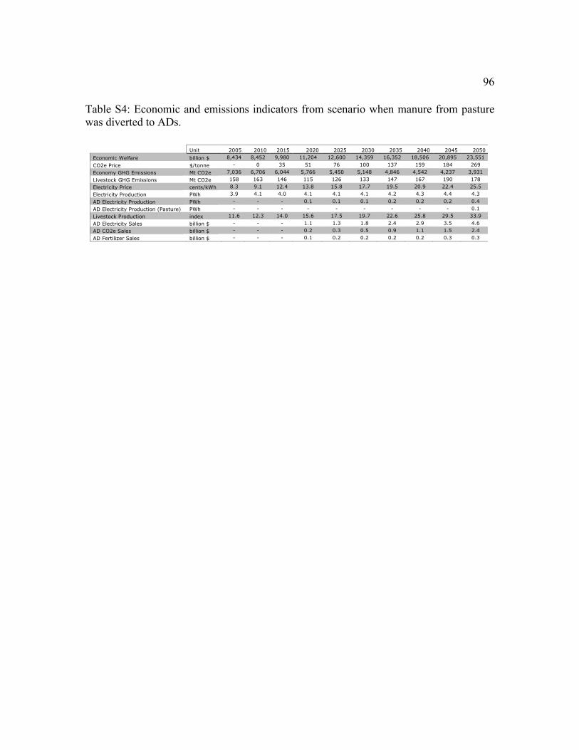
96  

Table S4: Economic and emissions indicators from scenario when manure from pasture was diverted to ADs.

Unit 2005 2010 2015 2020 2025 2030 2035 2040 2045 2050 Economic Welfare billion $ 8,434 8,452 9,980 11,204 12,600 14,359 16,352 18,506 20,895 23,551 CO2e Price $/tonne - 0 35 51 76 100 137 159 184 269 Economy GHG Emissions Mt CO2e 7,036 6,706 6,044 5,766 5,450 5,148 4,846 4,542 4,237 3,931 Livestock GHG Emissions Mt CO2e 158 163 146 115 126 133 147 167 190 178 Electricity Price cents/kWh 8.3 9.1 12.4 13.8 15.8 17.7 19.5 20.9 22.4 25.5 Electricity Production PWh 3.9 4.1 4.0 4.1 4.1 4.1 4.2 4.3 4.4 4.3 AD Electricity Production PWh - - - 0.1 0.1 0.1 0.2 0.2 0.2 0.4 AD Electricity Production (Pasture) PWh - - - - - - - - - 0.1 Livestock Production index 11.6 12.3 14.0 15.6 17.5 19.7 22.6 25.8 29.5 33.9 AD Electricity Sales billion $ - - - 1.1 1.3 1.8 2.4 2.9 3.5 4.6 AD CO2e Sales billion $ - - - 0.2 0.3 0.5 0.9 1.1 1.5 2.4 AD Fertilizer Sales billion $ - - - 0.1 0.2 0.2 0.2 0.2 0.3 0.3

!

97  

Table S5: Economic and emissions indicators from scenario when flaring is available in addition to electricity generation by ADs.

Unit 2005 2010 2015 2020 2025 2030 2035 2040 2045 2050 Economic Welfare billion $ 8,434 8,452 9,982 11,206 12,607 14,371 16,369 18,525 20,913 23,565

CO2e Price $/tonne - - 33 54 78 106 135 160 185 275

Economy GHG Emissions Mt CO2e 7,036 6,706 6,045 5,719 5,398 5,081 4,767 4,451 4,133 3,811

Livestock GHG Emissions Mt CO2e 158 124 97 107 117 130 148 168 191 152

AD GHG Mitigation Mt CO2e - - - - - 26 69 78 89 114

Flaring GHG Mitigation Mt CO2e - 44 50 56 62 44 12 14 16 6

Electricity Price cents/kWh 8.3 9.1 12.2 14.0 15.9 18.1 19.4 21.0 22.5 25.8

Electricity Production PWh 3.9 4.1 4.0 4.1 4.1 4.1 4.2 4.3 4.4 4.4

AD Electricity Production PWh - - - - - 0.1 0.1 0.2 0.2 0.2

Livestock Production index 11.6 12.3 14.1 15.8 17.6 19.8 22.7 26.0 29.7 33.8

AD Electricity Sales billion $ - - - - - 0.7 2.1 2.5 3.0 4.4

AD CO2e Sales billion $ - - - - - 0.2 0.7 1.0 1.3 2.4

AD Fertilizer Sales billion $ - - - - - 0.1 0.2 0.2 0.2 0.3

!

98  

Table S6: Economic and emissions indicators from scenario with an increase of 30 percent mitigation from ADs.

Unit 2005 2010 2015 2020 2025 2030 2035 2040 2045 2050 Economic Welfare billion $ 8,434 8,452 9,980 11,204 12,601 14,362 16,355 18,508 20,901 23,560

CO2e Price $/tonne - - 35 51 76 99 131 159 184 274

Economy GHG Emissions Mt CO2e 7,036 6,706 6,044 5,719 5,396 5,081 4,767 4,451 4,133 3,811

Livestock GHG Emissions Mt CO2e 158 163 146 101 102 114 124 141 161 144

Electricity Price cents/kWh 8.3 9.1 12.4 13.8 15.8 17.7 19.3 20.9 22.4 25.7

Electricity Production PWh 3.9 4.1 4.0 4.1 4.1 4.1 4.2 4.3 4.4 4.4

AD Electricity Production PWh - - - 0.09 0.12 0.13 0.16 0.19 0.21 0.24

AD Electricity (1000kW) PWh - - - 0.09 0.11 0.12 0.14 0.16 0.18 0.21

AD Electricity (500kW) PWh - - - - 0.01 0.01 0.02 0.02 0.02 0.02

AD Electricity (250kW) PWh - - - - - - 0.01 0.01 0.01 0.01

Livestock Production index 11.6 12.3 14.0 15.7 17.5 19.8 22.8 26.2 29.9 34.2

AD Electricity Sales billion $ - - - 1.1 1.5 1.8 2.4 2.9 3.6 4.6

AD CO2e Sales billion $ - - - 0.3 0.5 0.7 1.1 1.5 1.9 3.3

AD Fertilizer Sales billion $ - - - 0.1 0.2 0.2 0.2 0.3 0.3 0.3

!

99  

Figure S1: Production structure for ADs in the EPPA model.

Manure - Capital - Labor - Transport

Digester Production

Other Industry

Electricity Fertilizer CO2e allowances

Manure resource Transport

Capital - Labor

Capital Labor

kl

100  

Figure S2: U.S. Electricity generation in reference (a) and policy-no digesters (b) scenarios. Note: Advanced fossil includes natural gas combined cycle (NGCC), NGCC with sequestration, integrated gasification with combined cycle and sequestration, and wind with gas backup.

0

2

4

5

7

2005 2015 2025 2035 2045

Elec

trici

ty G

ener

atio

n (P

Wh)

Year

Fossil Fossil Advanced Fossil / Nuclear

Advanced Fossil / Nuclear Renewable Renewable

0.0 Coal 48.8 Advanced Fossil

9.6 Hydro

0.0 Gas 25.0 Nuclear 16.6 Wind

0.0 Oil 0.0 Bioelectric

Legend values are percent of electrical generation in 2050

Legend values are percent of electrical generation in 2050

Legend values are percent of electrical generation in 2050

Legend values are percent of electrical generation in 2050 - Reduced Use

0

2

4

5

7

2005 2015 2025 2035 2045

Elec

trici

ty G

ener

atio

n (P

Wh)

Year

Fossil /Nuclear

Fossil /Nuclear Renewable Renewable

54.4 Coal 4.1 Hydro14.8 Gas 8.2 Wind3.5 Oil 0.0 Bioelectric15.1 Nuclear Legend values are percent of

electrical generation in 2050Legend values are percent of electrical generation in 2050

a) b)

101  

Chapter 4

Data and Monitoring Needs for a More Ecological Agriculture

Zaks DPM, CJ Kucharik (submitted) Environmental Research Letters.

Abstract

Information on the life-cycle environmental impacts of agricultural production is often

limited. As demands grow to increase agricultural output while reducing its negative

environmental impacts, both existing and novel data sources can be leveraged to provide

more information to producers, consumers, scientists and policy makers. We describe the

components and organization of an agroecological sensor web. This web integrates

remote sensing technologies and in-situ sensors with models in order to provide decision

makers with effective management options at useful spatial and temporal scales. Several

components of the system are already in place, but by increasing the extent and

accessibility of information, decision makers will have the opportunity to enhance food

security and environmental quality. Potential roadblocks to implementation include

farmer acceptance, data transparency, and technology deployment.

102  

4.1 Introduction

The global agricultural system has provided food, feed, fiber and fuel to a population that

has quadrupled over the past century. While output of agricultural products has increased

over time, so too have negative environmental impacts (MEA 2005, Foley et al 2005).

The market prices of most agricultural goods produced today do not reflect the life-cycle

environmental impacts of production, transportation and consumption. Such information

must be available if we are to have a more informed market, one that internalizes the

environmental costs of agricultural production currently borne by society.

The challenge to provide for a larger, more affluent population in the coming decades

while decreasing the environmental impacts of agriculture is increasingly clear to both

scientists and policymakers (The World Bank 2008, Federoff et al 2010, Godfrey et al

2010). Improved monitoring and dissemination of data about the status and trends of

agroecosystems are needed if agricultural products are to be delivered with smaller

environmental footprints and if their prices are to reflect the life-cycle costs of

production.

Farmers and land managers have become the de facto managers of the largest anthrome,

on earth - agroecosystems (Ellis and Ramankutty 2008). Often they do not have the

proper resources for managing agroecosystems to maximize productivity and deliver

ecosystem services simultaneously. In most cases, farmers make management decisions

103  

based on assessment of local conditions, previous experience and desired outcomes.

Their knowledge can be supplemented with management recommendations derived from

satellites, on-the-ground sensors and computer models that monitor and help forecast

environmental conditions and crop needs. These new observations are like an added "pair

of eyes" that can help improve management decisions (Porter et al 2009). Limited

examples of this adaptive management cycle exist where precision agriculture (PA) tools

have been adopted, but there is a need for improved monitoring and information

dissemination infrastructure (Bramley 2009, Lindenmayer and Likens 2010).

While the whole structure of an improved agroecological monitoring system has yet to be

designed, researchers in both public and private sectors are currently developing many

elements. These elements bridge remote sensing and ground based monitoring systems

with real-time, smart, wireless, Internet connected sensor webs (Rundel et al 2009,

Adamchuck et al 2004). New technologies can assist in analysis and reporting of spatial

and temporal variability across the agroecological landscape (McLaren et al 2009, Hale

and Hollister 2009). With these new data streams, systems must be designed to aggregate,

coordinate, organize and synchronize within and between monitoring networks.

Restructuring the current agroecological monitoring and analysis systems will not only

require new technologies, but cooperation between governments, academia, private

industries and farmers as well. Policy and economic incentives that explicitly value

104  

public goods will be vital to the success of any system. To overcome these challenges, an

innovative multidisciplinary approach that leverages the available tools to deliver a more

ecologically sound agriculture will be required. The momentum needed to implement this

type of system can be initiated by policies to reduce the life cycle impacts of agricultural

production. This will require a more robust system to collect, analyze and disseminate

data on the functioning of the agricultural system. Putting these data in the hands of

decision makers has the potential to decrease environmental impact while increasing

efficiency of production.

There are many challenges related to sustainability to be addressed at the intersection of

science and technology, agriculture, and policy. Availability of data on the dynamics of

the agroecological system will be necessary to inform decision-makers at the forefront of

increasing the sustainability of these systems. Here we review the state of on-going

monitoring activities and propose pathways to implement an enhanced agroecological

monitoring system that can assist producers, consumers, policy makers and scientists to

make more informed decisions at the interface of the food system and environment.

4.2 Gaps in tools currently used to facilitate decisions in the agricultural sector

Predicting the impact of the global food system on the environment requires data on

system functioning, responses to change, and the potential impacts of management

decisions. Development of extensive datasets and numerous models has been

105  

progressing, although enhancements in data collection methodology, aggregation and

dissemination are necessary to meet both production and environmental goals. Gaps in

the patchwork of currently available data, models and indicators must be filled to attain

an adequate agricultural monitoring system (O'Malley et al 2009).

4.2.1 Ground-based and Remote Data Collection

Observations of agroecosystems monitor changes in agricultural or ecosystem processes,

but seldom both (Lovett et al 2007). Commonly collected production data include the

crop type (McNairn et al 2009), phenology/ crop progress (Sakamoto et al 2005), area

covered (Ramankutty et al 2008), and yield (Monfreda et al 2008, Wang et al 2010, Ross

et al 2008). The U.S. Department of Agriculture's Foreign Agriculture Service provides

agrometerorological data through their Crop Explorer tool that integrates stations, models

and satellites on a regional scale (USDA 2010). Other satellite systems, such as SPOT,

can be contracted to provide imagery that assists in monitoring a range of agricultural

parameters. The spatial and temporal scales at which remote sensing and ground-based

monitoring are conducted are seldom coordinated, which can hamper efforts to synthesize

crop data at regional and global scales.

Environmental field data most often collected include quantification of soil water

(Robock et al 2000, Zhang et al 2010), greenhouse gases (Baldocchi 2008, Bréon and

Ciais 2010) and nutrient cycling (Batjes 2009). However, environmental data collection

106  

methods in agroecological landscapes vary based on the scale of interest and intended

purpose. Irrigated areas can be detected from satellites, but on-farm water use data are

best collected at the field scale. Fertilizer use (or run-off) can be calculated through

production, sales data and application records, but these data are not often spatially

referenced. Mapping of the global distribution of fertilized lands has only recently been

accomplished (Potter et al 2010). Integrated monitoring of crop input needs and

environmental variables is rarely undertaken in unison.

4.2.2 Models

Models are useful tools for synthesizing data, simulating the relationship between

environmental conditions and agroecosystem variables, and exploring such scenarios as

potential management decisions, climate change, increased atmospheric CO2, and their

impacts. Model output can sometimes replace field data when data collection is too

costly, impractical or time consuming. Models can also be used to project the end of

season field conditions based on initialization with field data and scenarios of seasonal

weather. Some models are designed on first principles and validated by field data, while

others are designed to reproduce the variability seen in observations. Agronomic models

that use input data (soils, climate, etc.) in order to perform simulations rely both on the

underlying structure of the model and on the quality of the input data. Therefore, if input

data are limited or of poor quality, the model results may be inaccurate. Many models

107  

report a static set of results, but Internet models can produce user-generated simulations

on the fly (Eckman et al 2009).

There are three general modeling frameworks to simulate the components of the

agricultural system that range in scale and complexity. Detailed crop models, like

DSSAT, are used in both research and management activities (Jones et al 2003).

Agroecosystem models, like Agro-IBIS and LPJ-mL, incorporate crop specific modules

into existing models designed to study the interactions of ecosystems with environmental

drivers of change (Kucharik 2003, Bondeau et al 2007). Integrated models, such as

IMPACT and BLS, incorporate socioeconomic parameters into environmental and

agronomic relationships to simulate the broader food system (Rosegrant et al 2008, Parry

et al 2004). Given this variety of tools, there are many opportunities to improve the data

flow between agroecological sensors, models, and users can benefit from the value-added

output to improve the decision-making processes.

4.2.3 Indicators

In lieu of real-time data on the functioning of agroecosystems, a variety of indicators

have been developed to relay information about the state of a system and how it might be

changing. The Heinz Center (2008) defines an indicator as "a specific, well-defined, and

measurable variable that reflects some key characteristic that can be tracked through time

to signal what is happening within and across ecosystems." Data collected at various

108  

spatial and temporal scales are used as inputs for indicators, but the use of an indicator

can mask the complexity of a system (Payraudeau 2005). Current sets of indicators are

useful, as they can assist in targeting regions and variables that are poorly monitored. The

Heinz Center developed a thorough set of indicators for United States ecosystems, but

adequate data existed to calculate only 30 percent of indicators, while another 30 percent

had partial data, and 40 percent of indicators had insufficient data for calculation (Heinz

2008). The Organisation for Economic Co-operation and Development (OECD) created

indicators for the environmental performance of agriculture for their 30 member states

(OECD 2008). Of the 37 indicators they developed, only 20 (54 percent) were deemed to

be scientifically sound; on average, 18 of the 30 countries (60 percent) had adequate data.

The paucity of data available to activate indicators further highlights the need for

improved data collection, standardization and distribution.

4.3 Improvements in agroecological monitoring systems

Improved monitoring and integrated decision making can help overcome many of the

challenges that face the agroecological system. Many of these technologies are already

available (Gebbers and Adamchuk 2010), but have seldom been incorporated in a

systematic manner. Benefits from enhanced observations are likely to emerge when

monitoring networks, reporting across different spatial and temporal scales, are integrated

so as to reveal novel system behaviors. We propose that relaying these data and trends to

109  

decision makers in the field, or those crafting policy can bring about a positive feedback

loop which can help achieve desired production and environmental outcomes.

Agroecosystems not only have their own ecological behavior, they are embedded within

ecologies at larger scales. We suggest that monitoring should encompass the nested

scales at which decisions are made across agroecological systems. These systems respond

to drivers across many dimensions of space and time; from daily variation in soil

micronutrients within a field to changes in weather over days and seasons, and climate

changes over decades. Monitoring current conditions gives decision makers the ability to

manage with greater precision, while documenting trends over a longer length of time can

help reveal potential thresholds and discontinuities, and assist in both short-term forecasts

(e.g. end of season yields) and long-term adaptations. On-farm monitoring systems and

portable imaging systems should be able to capture differences within and between fields,

while earth-orbiting systems can obtain a broader perspective of changes. The integration

of ground-based monitoring networks with remotely sensed data has the potential to offer

added value to scientists and decision makers alike.

At the farm scale, data from enhanced monitoring will likely be used if it is presented in a

form that is easily integrated into existing decision-making structures (Kitchen 2008). If

data from on-the-ground and remote systems is going to be utilized by several parties

(e.g. farmers, scientists, policy makers, consumers), additional infrastructure will be

110  

needed to aggregate, process, store and disseminate data products. Wireless systems are

already in place, at a small scale, to aggregate data from several monitors within a field

(Wang et al 2006), and for satellite systems (Duveiller and Defourny 2010). However,

more robust technology will be needed to transform raw data into useful products, and

thereby ensuring effectiveness. Standards-based data transfer protocols from Open

Geospatial Consortium (Nash et al 2009; Kooistra et al 2009) have been developed to

seamlessly integrate multiple data sources.

To be effective, an agroecological monitoring system must capture changes over a range

of processes. While crops in different biomes have individual biotic and abiotic needs, a

general framework for monitoring needs can still be assembled. Agricultural inputs

including fertilizers and water as well as yield form the basis of productivity

measurements. Records of crop varieties, planting extent and timing are also useful to

treat food security issues. Ecological indicators such as soil type and fertility and

meteorological indicators such as solar radiation and humidity help us understand longer-

term production and environmental changes.

These data are the basic building blocks needed to ensure that the timing, magnitude and

location of management decisions have the desired agroecological outcomes. The spatial

scale and frequency of data collection will vary depending on the needs of the manager,

with more frequent temporal data and greater spatial resolution preferred. The regional to

111  

continental extent of monitoring activities must include well-managed, highly productive

systems as well as those in sub-optimal locations or with limited management in order to

capture the full range and responses of agronomic and environmental variables.

Environmental sensor technology has continued to improve because of increased

availability and sensor capacity and decreased cost. Given the extensive nature of

agriculture, sensors capable of providing data at spatial and temporal scales useful to on-

the-ground managers have been increasingly adopted (Lamb et al 2008). These improved

sensors take advantage of innovations in data collection technology, data transfer

capabilities between sensors and to the Internet, on-the-fly data processing, and

renewable and energy efficiency technologies (e.g. Pierce and Elliot 2008, Sun et al

2009, Conover et al 2009). This portends reduced monitoring costs, increased data

availability, better spatial and temporal measurement scales and the ability to monitor

more components.

4.3.1 Soil physical and chemical properties

Soil sensors to monitor nutrients, physical properties and sub-surface dynamics are

already available. A range of sensors exist depending on the variable in question and

includes electrical, optical, mechanical, acoustic, pneumatic and electrochemical types

(Adamchuck et al 2004). Optical methods have shown the most promise for nutrient

sensing (Sinfield et al 2010). Observation of the correlations between primary properties

112  

of optical sensing and quantities such as pH, cation exchange capacity and microbial

activity have been documented (Nduwamungu et al 2009, Allen et al 2007). While the

majority of soil sensors are ground-based, airborne hyperspectral imaging has been used

to measure soil organic carbon (Stevens et al 2010). In comparison to traditional in-lab

soil testing, these new approaches have been shown to reduce costs as much as 80 percent

(Nduwamungu et al 2009, Wang et al 2006, Kim et al 2009), and do not require

disturbing the soil structure (Serrano et al. 2010). The accuracy of some measurements is

not as great as their laboratory counterparts, but their increase in sampling resolution,

decrease in cost and synergy with other management activities has led to their increased

acceptance (Christy et al 2008).

4.3.2 Water

Monitoring soil moisture status, coupled with vegetation vigor, is necessary in order to

understand how cropping systems respond to highly variable soil moisture conditions. In

irrigated systems, crop water needs require higher resolution data than those commonly

used so that water is provided in a more efficient manner given heterogeneous soil

conditions (Greenwood et al 2010, Sadler et al 2005). Soil moisture sensors have been

developed for below-ground, above-ground and remote monitoring. Champagne et al

(2010) used a ground-based network to test the ability of a satellite-based passive

microwave sensor with promising results. Data from in-ground soil moisture and

temperature sensors in a cotton field were transmitted via radio frequency identification

113  

(RFID) chips to a central processor to assist in site-specific irrigation scheduling (Vellidis

et al 2008). A ground-based optical remote sensing system was fixed to a center-pivot

irrigation site to provide in-situ measurements. These were used to compute a water

deficit index, thus improving irrigation decisions (Colaizzi et al 2003).

4.3.3 Crop Identification

Crop identification and yield monitoring data can be used to advise markets on crop

production and progress, and for food security related questions, input to models, and on-

farm management (Blaes et al 2005). Current approaches for crop identification across

large areas use optical sensors, radar sensors, or a combination of the two (McNairn et al

2009). Jang et al (2009) used a series of Landsat images supplemented with the MODIS

normalized difference vegetation index (NDVI) to discriminate between crop types with

success. McNairn et al (2009) used a combination of optical sensors (SPOT and Landsat)

and radar (RADARSAT and ASAR) for individual crop classifications across Canada

with accuracies of 80-90 percent. Yield can be estimated from monitoring sensors located

on the tractor (Ross et al 2008), or combined with satellite images (which have been

calibrated with in situ data) for a broader spatial coverage (Doberman and Ping 2004).

Satellite remote sensing images can be used in conjunction with yield-forecasting models,

but often need on-the-ground validation (Wang et al 2010).

114  

4.3.4 Processing and Visualization

Data collected by in-situ or remote sensors are rarely useful by themselves in decision-

making either on or off the farm. Integrating this information with other observations and

models, and then effectively communicating it to the decision maker can help to fully

leverage these new data sources. Emerging systems include features such as on-the-fly

error correction and modeling and the distribution of results to the Internet or cellular

phones. The Intelligent Sensorweb for Integrated Earth Sensing combines in situ

measurements, crop growth models and online maps of predicted crop and range yields

and transmits the product to managers (Teillet et al 2007). In South Africa, where the

internet is less accessible, Singels and Smith (2006) report on a system to provide advice

on irrigation scheduling to small-scale sugarcane farmers via cell phone, a technology

that is much more readily available. Similarly, Antonpoulou et al (2009) created a

personalized spatial model that incorporates policy, market, environmental, and

agronomic information to the user via cell phone in Greece. In areas where

agroecological monitoring may not be available, web crawlers can "mine" data from

websites to provide information on the changing state of the system (Galaz et al 2009).

4.3.5 Agroecological Sensor Webs

The monitoring systems described here have been deployed for decision making at the

farm and regional scales. The advent of internet-connected real-time wireless sensors

presents a new opportunity to integrate data from a wide variety of sources. These sensor

115  

webs can exhibit emergent properties of the agricultural system that may not have been

otherwise observable (van Zyl et al 2009). New tools are required for data organization,

synthesis and integration as data become available from individual networks across the

agroecological landscape (Hale and Hollister 2009) (Figure 1).

As the amount of data produced by environmental and ecological sensor systems has

grown, techniques in database management, informatics, statistics, spatial processing and

visualization have emerged to meet the challenge of data handling, processing and

storage (e.g. McLaren et al 2009, Uslander et al 2010, Ball et al 2008, Jurdak et al 2008).

For the most part, these new techniques have emerged at the fringes of traditional

disciplines, for example, by bringing together biologists and computer scientists to

contribute new tools (Benson et al 2010). Many of these tools can be applied to building

an agroecological sensor web, if the data are used as model input, and the model output is

rapidly disseminated directly to the decision maker.

4.4 Discussion

The limitation to implementing an enhanced agroecological monitoring system is not the

sensor technology; rather it is leveraging the output data for decision-making on several

levels that would reduce the negative impacts of agriculture on the environment. Unlike

the current approach of precision agriculture, agroecological data must be paired with

innovative policies if the simultaneous production and environmental goals are to be met.

116  

Data from agroecological monitoring can be used throughout the supply chain of

products, from producers and consumers to policy-makers and scientists.

4.4.1 Producers

Technology vendors, scientists and policy makers can extol the virtues of sensor web

technology ad nauseam, but results will be limited to scientific results until a significant

proportion of the agricultural community adopts it. For producers in developing

countries, here is an opportunity to leapfrog the traditional development pathways and

adopt the latest methods and technologies. But the acceptance of precision agriculture

technology has been relatively slow thus far (Daberkow and McBride 2003, Sumberg

2005). One strategy to avoid falling from the "peak of inflated expectations" to the

"trough of disillusionment" of technology adoption, as described by Lamb et al (2008) is

to ensure the delivery of decision-relevant information to the producer, compared to raw

data which has limited usefulness. Before too much hype is made about the many

potential benefits of agroecological sensor webs, the systems sensor data need to be

incorporated into decision support systems that allow the producer to explicitly

understand potential trade-offs between management decisions and ecological and

production outcomes (Fountas et al 2006). While some systems are in development,

additional work is needed to ensure the transparency, reliability and ease-of-use of the

software and its integration into current agricultural management tools. Once these

117  

objectives are met, there is a higher likelihood that a rapid adoption of agroecological

sensor webs will ensue.

4.4.2 Consumers

Eco-labels and certifications are emerging as an approach to inform consumers about the

products they purchase. Labels for products such as organic foods, sustainable wood

products and energy-saving appliances have been growing in recent years (Ibanez and

Grolleau 2008, Kotchen 2006). Additional food labels provide information on how the

items were produced, such as fair-trade, shade-grown or dry-farmed (Howard and Allen

2010). While comparisons can currently be made between products with eco-labels and

those without, little specific information is communicated to the consumer about the life-

cycle impacts. As supply chains shift to increase the transparency of their products, data

from agroecological sensor webs can be used to communicate the back-story of the

product to the consumer (Opara and Mazaud 2001). Building on the success of other eco-

labels, Faludi (2007) proposed "eco-nutrition" labels that mimic the current labels on

food products (Figure 2). These labels would communicate energy, resource, water,

toxins and social scores of the product's life-cycle to the user and would allow for more

in-depth comparisons among products. Similar graded eco-labels can provide consumers

with information on multiple environmental performance indicators (Bleda and Valente

2009). Labels like these could be improved with enhanced agroecological sensor web

technology.

118  

4.4.3 Science

Many of the models that simulate crops, ecosystems and economies are hampered by a

scarcity of data about the system of interest. Limitations in computing power to run the

simulations are being lifted as computers have become cheaper and more powerful.

Integration of new data at higher spatial and temporal resolution, supplemented by

historical data, can improve the precision and accuracy of model output. In addition, new

streams of multivariate and multidisciplinary data will require the expertise of many

disciplines to unravel the agroecological complexities veiled under the many new layers

of information.

While new data streams, such as those from an agroecological sensor web, may assist in

further refining these models, they can also help to elucidate previously unknown or

poorly understood relationships within the modeled system. Some newly collected data

may not even fit into the structure of current models, and in this case new models will

need to be built that can harness an input dataset with increased dimensionality over time

and space. These new models can also help to create links between disciplines, especially

in the physical and social sciences that are needed to solve problems and produce

solutions for policy makers. These systems can also help to strengthen partnerships

between developed and developing countries and foster the co-development of new

models and knowledge sharing.

119  

4.4.4 Policy

At the most basic level, the interactions between policy makers and the agricultural

system occur both at the marketplace and through the regulatory structure. Broad polices

such as the U.S. Department of Agriculture Conservation Reserve Program and markets

for ecosystem goods and services have similar goals of striking a balance between

production of agricultural goods and protection of vital ecosystem services. However,

they must often rely on generalized information that lacks a connection between a parcel

of land and its delivery of ecosystem goods and services. By incorporating data from

agroecological sensor webs into a policy framework, a structure can be developed to

provide incentives for lands that produce a suite of ecosystem goods and services, as well

as the ability to value these services separately. These incentives can be modified

according to updated data, an improvement on a program that values all areas equally.

In the near term, the fundamental data gap in need of attention is the monitoring of

greenhouse gases (GHG) from agricultural lands. As policies are negotiated to reduce

GHGs across the U.S. economy, emissions from agriculture may be excluded from a cap-

and-trade system because they are hard to measure, monitor and verify (Smith et al 2007,

Dale and Polasky 2007). The added transaction costs, and uncertainty in emissions

reductions, have marginalized the 7 percent of U.S. GHGs emitted by agricultural

activities (EPA 2010). Improved monitoring of carbon dioxide, nitrous oxide and

120  

methane from agriculture could provide the information and incentives necessary for

carbon markets, policy makers and farmers to reduce emissions from the production life

cycle.

4.4.5 Getting From Here to There: Innovation, Investment and Transparency

Many of the technologies highlighted here have yet to be deployed at the scale necessary

to display the emergent properties of an agroecological sensor web (Table 1). As the

focus on agricultural innovation shifts to incorporate both production and environmental

objectives, information and communications technologies (ICT) are likely to play a larger

role. As investments and technological breakthroughs in ICT have generally been focused

on sectors other than agriculture, there is tremendous potential to apply the technology

already available to agroecological uses (Sassenrath et al 2008). Important advances are

likely in approaches to transmit, store, process and aggregate data from multiple sources

to aid in site-specific decision-making.

Sensor webs have already emerged at several spatial scales. Examples include the Global

Earth Observing System of Systems (Justice et al 2007), National Ecological Observatory

Network (Keller et al 2008) and Chesapeake Bay Environmental Observatory (Ball et al

2008). These systems are driven by their own science questions and can serve as useful

building blocks to address new agroecological questions. Like these examples, an

agroecological sensor web will require the buy-in and support from many entities,

121  

expanding beyond the public sector. While the metrics for success will be variable,

explicit goal setting amongst sensor web partners will be necessary to avoid unrealistic or

unattainable goals.

The cost of installing an agroecological monitoring system is likely to vary as a function

of the area covered, the variables tracked and the degree of integration with other

systems. The diversity of potential stakeholders and end-users of the data introduces a

variety of actors to help burden the cost of such a system and help bring it to fruition.

Even with high initial capital costs, the benefits are likely to be high. Private benefits can

include increased yields and decreased costs from inputs; public benefits include

increased availability of ecosystem services from biodiversity, carbon sequestration, and

water infiltration. Public and private investments will be essential to realize these benefits

(Alston et al 2009).

The availability of data on how management decisions affect the provision of ecosystem

goods and services can help to inform markets and offset the costs of monitoring

(Swinton et al 2007, Dale and Polasky 2007). Tracking changes in production and

ecosystem service delivery facilitates the internalization of costs from agriculture that

were previously external. While developing these markets will require outside capital, as

markets grow they should provide returns that help to build additional monitoring

capacity.

122  

The increased availability in wireless monitoring devices is not limited to the agricultural

sector, but examples can be found in cell phone photography and closed caption

television systems (Dennis 2008). The public availability of these new data streams has

had a positive social benefit since they act as a deterrent for "anti-social behaviors"

(Ganascia 2010). The rise of sousveillance, where societal monitoring activities are

becoming widespread and data are publicly available, has yet to be explored for

agricultural applications. If the maximum benefit of sensor web technology is to be

realized, then the data collected will need to have both on- and off-farm uses.

To date, most data collected on-farm for management purposes is not used in other ways

and scientific and census data are usually collected independently. The U.S. National

Agricultural Statistics Survey (NASS) promotes "confidentiality and data security" in

regard to data about agricultural production. With additional production and

environmental data being potentially readily available, making all collected data publicly

available and transparent has its merits. Consumers will be able to trace the origins of

their products and monitor the conditions under which they were produced. This will

compel producers to improve the environmental performance of their products. Increased

transparency in the agricultural system can close the gap between producers and

consumers through the monitoring and open distribution of agroecological data.

123  

4.5 Conclusions

The grand challenge for agriculture over the next forty years is to reduce its

environmental impact while producing enough food, feed and fiber for a larger and

wealthier population (Robertson and Swinton 2005). While the first green revolution

brought increases in productivity, these carried environmental costs and the next

generation of farmers will be in the vanguard to reduce those impacts. This cohort will be

an increasingly digitally connected group and will have access to unprecedented amounts

of data. As new farmers will be recruited into an occupation that has steadily decreased in

size over the past generation, the image of the farmer needs to be recast as a 21st century

steward of the land, equipped with digital tools, knowledge and skills to meet

increasingly stringent multi-functional demands.

Moving enhanced agroecological monitoring from research lab to farm field will take

commitments and investments from a diverse array of stakeholders (Sachs et al 2010).

Not only are there many technical elements in need of further development in the

proposed system, but also the agricultural sector has an internal dynamic that has stifled

other potentially important innovations. Therefore the social, economic and

environmental stakeholders in the system will need to be on board before a successful

introduction is possible.

124  

The opportunity to establish a global agroecological monitoring system comes at a time

when increasing agricultural demands and reducing environmental impacts from

production have gained attention at the highest political levels. While this is a formidable

challenge, we have recently entered an era where monitoring, data processing and

communications technologies have the ability to give agroecological decision making

new dimensions. Policies that provide incentives to create these new data streams and

leverage their data to put an objective value on the ecosystem goods and services

connected to agriculture are paramount. While the investment needed for such a system is

large, the return on investment, as measured by agricultural productivity and reduced

environmental impacts, can be great as well.

125  

Acknowledgements

The authors would like to thank George Allez, Sam Batzli and Carol Barford for their

useful comments and suggestions, and Jeremy Faludi for allowing us to adapt a version

of Figure 2 for use in the manuscript. Images from Figure 1 are credited (from L to R),

D.P.M.Z., and flickr users stawarz, ostrosky and ciat. D.P.M.Z. was supported by the

National Science Foundation grant 144-144PT71 and C.J.K. was supported by the

National Aeronautics and Space Administration's Interdisciplinary Earth Science

Program.

126  

Table 1: Summary of the current and potential future components of an agroecological sensor web.

Current Future

Markets for food, carbon and other EGS

Carbon markets limited by lack of available data; Nutrient markets in their infancy

Markets informed by data from agroecological sensor web

In-situ & remote monitoringYield monitoring becoming common in high-

input systems, remote sensing algorithm output not explicitly designed for agricultural users

Access to data available to on-farm decision makers via internet and cellular

phones in real-time

Data transparency Limited public availability of data Agricultural sousvelliance joins other emerging monitoring systems

Product labeling Product certification labeling lacks differentiation between impact categories

Products assigned grades based on water, carbon, nutrient, biodiversity

impacts

Scientific models Models driven & validated by limited observations

Social, economic and environmental data streams used to constantly update

model validation and modify projections

Impacts of production 60% of ecosystem services negatively impacted by agriculture

Reduced environmental impacts, increased food security

Social and environmental costs of production

External to product cost Internalized in product cost

127  

Figure 1:

Major components of the agroecological sensor web. Individual sensors including remote

(e.g. satellite, aircraft, unmanned drone), automated in-situ and direct human

observations collect data at multiple spatial scales. These data are processed for quality

control and data from multiple networks across spatial scales are aggregated. These data

are used as inputs to agronomic, agroecological and integrated models. The output of the

models can be used by producers for real-time management and long-term planning,

consumers to discriminate products based on their environmental footprints, scientists to

study the dynamics of agroecosystems and policy-makers to guide policies to further

reduce environmental impacts of agricultural production.

Data Processing

Aggregation

ModelIntegration

ModelOutput

Producer

Scie

nce

& P

olicy

Consum

er

AggregationAggregationAggregation

Management Feedbacks

Data-InformationTransition

Decision MakingData Collection

128  

Figure 2:

A representation of an eco-label that integrates data from several monitoring sources and

clearly communicates the life-cycle environmental impacts of the product to the

consumer. Figure adapted from Faludi (2007).

Environmental FactsOverall Weighted Score........................................... 5/10

Energy & Emissions

Resources

Toxins

Water

Social

Production Greenhouse Gases.......................... 3/10Transportation Greenhouse Gases..................... 7/10

Biodiversity.......................................................... 5/10Soil...................................................................... 4/10Air Quality............................................................ 6/10Nutrient Use........................................................ 3/10

Herbicide............................................................. 5/10Pesticide.............................................................. 5/10Other Toxins........................................................ 6/10

Embodied Water................................................. 2/10Water Pollution.................................................... 1/10

Labor Practices................................................... 8/10Transparency..................................................... 10/10

5

Worst Best

129  

References Adamchuk V, Hummel J, Morgan M and Upadhyaya S 2004 On-the-go soil sensors for precision agriculture Comput Electron Agr 44 71-91 Allen M F et al 2007 Soil sensor technology: Life within a pixel BioScience 57 859-67 Alston J M, Beddow J M and Pardey P G 2009 Agricultural research, productivity, and food prices in the long run Science 325 1209-10 Antonopoulou E, Karetsos S and Maliappis M 2009 Web and mobile technologies in a prototype DSS for major field crops Comput Electron Agr 70 292–301 Baldocchi D 2008 Breathing of the terrestrial biosphere: Lessons learned from a global network of carbon dioxide flux measurement systems Aust J Bot 56 1-26 Ball W P et al 2008 Prototype system for multidisciplinary shared cyberinfrastructure: Chesapeake bay environmental observatory J of Hydrol Engin 13 960-70 Batjes N H 2009 Harmonized soil profile data for applications at global and continental scales: Updates to the WISE database Soil Use Manage 25 124-7 Benson B J, Bond B J, Hamilton M P, Monson R K and Hans R 2010 Perspectives on next-generation technology for environmental sensor networks Front Ecol Environ 8 193-200 Blaes X, Vanhalle L and Defourny P 2005 Efficiency of crop identification based on optical and SAR image time series Remote Sens Environ 96 352-65 Bleda M and Valente M 2009 Graded eco-labels: A demand-oriented approach to reduce pollution Technol Forecast Soc Change 76 512-24 Bondeau A, Smith P C, Zaehle S, Schaphoff S, Lucht W, Cramer W and Gerten D 2007 Modelling the role of agriculture for the 20th century global terrestrial carbon balance Global Change Biol 13 679-706 Bramley R G V 2009 Lessons from nearly 20 years of precision agriculture research, development, and adoption as a guide to its appropriate application Crop Pasture Sci 60 197-217 Bréon F-M and Ciais P 2010 Spaceborne remote sensing of greenhouse gas concentrations CR Geosci 342 412-24

130  

Champagne C, Berg A, Belanger J, Mcnairn H and De Jeu R 2010 Evaluation of soil moisture derived from passive microwave remote sensing over agricultural sites in Canada using ground-based soil moisture monitoring networks Int J Remote Sens 31 3669-90 Christy C D 2008 Real-time measurement of soil attributes using on-the-go near infrared reflectance spectroscopy Comput Electron Agr 61 10-9 Colaizzi P, Barnes E, Clarke T, Choi C, Waller P, Haberland J and Kostrzewski M 2003 Water stress detection under high frequency sprinkler irrigation with water deficit index J Irrig Drain E-Asce 129 36-43 Conover H et al 2009 Using sensor web protocols for environmental data acquisition and management Ecol Inform 5 32-41 Daberkow S and Mcbride W 2003 Farm and operator characteristics affecting the awareness and adoption of precision agriculture technologies in the US Precis Agric 4 163-77 Dale V and Polasky S 2007 Measures of the effects of agricultural practices on ecosystem services Ecol Econom 64 286-96 Dennis K 2008 Keeping a close watch–the rise of self-surveillance and the threat of digital exposure Sociol Rev 56 347-57 Dobermann A and Ping J 2004 Geostatistical integration of yield monitor data and remote sensing improves yield maps Agron J 96 285-97 Duveiller G and Defourny P 2010 A conceptual framework to define the spatial resolution requirements for agricultural monitoring using remote sensing Remote Sens Environ 114 2637–2650 Eckman B, West P, Barford C and Raber G 2009 Intuitive simulation, querying, and visualization for river basin policy and management IBM J Res & Dev. 53 3 MEA (Millennium Ecosystem Assessment) 2005 Ecosystems and Human Well-Being (Washington, DC: Island Press) Ellis E C and Ramankutty N 2008 Putting people in the map: Anthropogenic biomes of the world Front Ecol Environ 6 439-47

131  

EPA 2010 Inventory of U.S. Greenhouse gas emissions and sinks: 1990 – 2008 Washington DC Faludi J 2007 Worldchanging: Bright green: The eco-nutrition label. Available online: http://www.worldchanging.com/archives/007256.html Federoff N et al 2010 Radically rethinking agriculture for the 21st century Science 327 833-4 Foley J et al 2005 Global consequences of land use Science 309 570-4 Fountas S, Wulfsohn D, Blackmore B, Jacobsen H and Pedersen S 2006 A model of decision-making and information flows for information-intensive agriculture Agr Sys 87 192-210 Galaz V, Crona B, Daw T, Bodin Ö, Nyström M and Olsson P 2009 Can web crawlers revolutionize ecological monitoring? Front Ecol Environ doi:10.1890/070204 Ganascia J 2010 The generalized sousveillance society Soc Sci Info 49 489 Gebbers R and Adamchuk V I 2010 Precision agriculture and food security Science 327 828-31 Godfray H et al 2010 Food security: The challenge of feeding 9 billion people Science 327 812-818 Greenwood D J, Zhang K, Hilton H W and Thompson A J 2010 Opportunities for improving irrigation efficiency with quantitative models, soil water sensors and wireless technology J Agr Sci 148 1-16 Hale S S and Hollister J W 2009 Beyond data management: How ecoinformatics can benefit environmental monitoring programs Environ Monit Assess 150 227-35 Heinz 2008 The State of the Nation’s Ecosystems. 2008 Howard P and Allen P 2010 Beyond organic and fair trade? An analysis of ecolabel preferences in the United States Rural Soc 75 244–269 Ibanez L and Grolleau G 2008 Can ecolabeling schemes preserve the environment? Environ Res Econ 40 233-49 Jones J, et al. 2003 The DSSAT cropping system model Eur J Agron 18 235-65

132  

Jurdak R, Nafaa A and Barbirato A 2008 Large scale environmental monitoring through integration of sensor and mesh networks Sensors 8 7493-517 Justice C and Becker-Reshef I 2007 Developing a strategy for global agricultural monitoring in the framework of group on earth observations (GEO), available online http://www.earthobservations.org/documents/cop/ag_gams/200707_01/20070716 _geo_igol_ag_workshop_report.pdf Keller M, Schimel D S, Hargrove W W and Hoffman F M 2008 A continental strategy for the national ecological observatory network Front Ecol Environ 6 282-4 Kim H-J, Sudduth K A and Hummel J W 2009 Soil macronutrient sensing for precision agriculture J Environ Monitor 11 1810-24 Kitchen N R 2008 Emerging technologies for real-time and integrated agriculture decisions Comput Electron Agr 61 1-3 Kooistra L, Bergsma A, Chuma B and De Bruin S 2009 Development of a dynamic web mapping service for vegetation productivity using earth observation and in situ sensors in a sensor web based approach Sensors 9 2371-88 Kotchen M 2006 Green markets and private provision of public goods J Polit Econ 114 816 Kucharik C J 2003 Evaluation of a process-based agro-ecosystem model (Agro-IBIS) across the US corn belt: Simulations of the interannual variability in maize yield Earth Interact 7 14 Lamb D W, Frazier P and Adams P 2008 Improving pathways to adoption: Putting the right P's in precision agriculture Comput Electron Agr 61 4-9 Lindenmayer D B and Likens G E 2010 The science and application of ecological monitoring Biol Conserv 143 1317-28 Lovett G M, Burns D A, Driscoll C T, Jenkins J C, Mitchell M J, Rustad L, Shanley J B, Likens G E and Haeuber R 2007 Who needs environmental monitoring? Front Ecol Environ 5 253-60 Mclaren C G, Metz T, Van Den Berg M, Bruskiewich R M, Magor N P and Shires D 2009 Informatics in agricultural research for development Adv Agron 102 135-57

133  

Mcnairn H, Champagne C, Shang J, Holmstrom D and Reichert G 2009 Integration of optical and synthetic aperture radar (SAR) imagery for delivering operational annual crop inventories J Photogram Rem Sens 64 434-49 Monfreda C, Ramankutty N and Foley J A 2008 Farming the planet: 2. Geographic distribution of crop areas, yields, physiological types, and net primary production in the year 2000 Global Biogeochem Cycles 22 GB1022 Nash E, Korduan P and Bill R 2009 Applications of open geospatial web services in precision agriculture: A review Precis Agric 10 546-60 Nduwamungu C, Ziadi N, Parent L-E, Tremblay G F and Thuries L 2009 Opportunities for, and limitations of, near infrared reflectance spectroscopy applications in soil analysis: A review Can J Soil Sci 89 531-41 O'malley R, Marsh a S and Negra C 2009 Closing the environmental data gap Issues Sci Technol 25 69-74 OECD 2001 Environmental indicators for agriculture Volume 3 methods and results 1- 400 Opara L and Mazaud F 2001 Food traceability from field to plate Outlook Agr 30 239-47 Parry M, Rosenzweig C, Iglesias A, Livermore M and Fischer G 2004 Effects of climate change on global food production under SRES emissions and socio-economic scenarios Global Environ Chang 14 53-67 Payraudeau S and Van Der Werf H 2005 Environmental impact assessment for a farming region: A review of methods Agr Ecosyst Environ 107 1-19 Pierce F J and Elliott T V 2008 Regional and on-farm wireless sensor networks for agricultural systems in eastern Washington Comput Electron Agr 61 32-43 Porter J H, Nagy E, Kratz T K, Hanson P, Collins S L and Arzberger P 2009 New eyes on the world: Advanced sensors for ecology BioScience 59 385-97 Potter P, Ramankutty N, Bennett E M and Donner S D 2010 Characterizing the spatial patterns of global fertilizer application and manure production Earth Interact 14 2

134  

Ramankutty N, Evan a T, Monfreda C and Foley J A 2008 Farming the planet: 1. Geographic distribution of global agricultural lands in the year 2000 Global Biogeochem Cycles 22 GB1003 Robertson G and Swinton S 2005 Reconciling agricultural productivity and environmental integrity: A grand challenge for agriculture Front Ecol Environ 3 38-46 Robock A, Vinnikov K, Srinivasan G, Entin J, Hollinger S, Speranskaya N, Liu S and Namkhai A 2000 The global soil moisture data bank B Am Meteorol Soc 81 1281- 99 Rosegrant M, Ringler C, Msangi S, Sulser T, Zhu T and Cline S 2008 A International model for policy analysis of agricultural commodities and trade (IMPACT): Model description. International Food Policy Research Institute, Washington, D.C. Ross K W, Morris D K and Johannsen C J 2008 A review of intra‐field yield estimation from yield monitor data Appl Eng Agric 24 309-17 Rundel P W, Graham E A, Allen M F, Fisher J C and Harmon T C 2009 Environmental sensor networks in ecological research New Phytol 182 589-607 Sachs J et al 2010 Monitoring the world's agriculture. Nature 466 558-60 Sadler E, Evans R, Stone K and Camp C 2005 Opportunities for conservation with precision irrigation J Soil Water Conserv 60 371-9 Sakamoto T, Yokozawa M, Toritani H, Shibayama M, Ishitsuka N and Ohno H 2005 A crop phenology detection method using time-series modis data Remote Sens Environ 96 366-74 Sassenrath G F, Heilman P, Lusche E, Bennett G L, Fitzgerald G, Klesius P, Tracy W, Williford J R and Zimba P V 2008 Technology, complexity and change in agricultural production systems Renew Agr Food Sys 23 285-95 Serrano J M, Peca J O, Marques Da Silva J R and Shaidian S 2010 Mapping soil and pasture variability with an electromagnetic induction sensor Comput Electron Agr 73 7-16

135  

Sinfield J V, Fagerman D and Colic O 2010 Evaluation of sensing technologies for on- the-go detection of macro-nutrients in cultivated soils Comput Electron Agr 70 1- 18 Singels A and Smith M T 2006 Provision of irrigation scheduling advice to small-scale sugarcane farmers using a web-based crop model and cellular technology: A South African case study Irrig Drain 55 363-72 Smith P, et al. 2007 Policy and technological constraints to implementation of greenhouse gas mitigation options in agriculture Agr Ecosyst Environ 118 6-28 Stevens A, Udelhoven T, Denis A, Tychon B, Lioy R, Hoffmann L and Van Wesemael B 2010 Measuring soil organic carbon in croplands at regional scale using airborne imaging spectroscopy Geoderma 158 32-45 Sumberg J 2005 Constraints to the adoption of agricultural innovations - is it time for a re-think? Outlook Agr 34 7-10 Sun Y, Li L, Lammers R S, Zeng Q, Lin J and Schumann H 2009 A solar-powered wireless cell for dynamically monitoring soil water content Comput Electron Agr 69 19-23 Swinton S M, Lupi F, Robertson G P and Hamilton S K 2007 Ecosystem services and agriculture: Cultivating agricultural ecosystems for diverse benefits Ecol Econom 64 245-52 Teillet P M, et al. 2007 An integrated Earth sensing sensorweb for improved crop and rangeland yield predictions Can J Remote Sens 33 88-98 The World Bank 2008 World Development Report: Agriculture for Development Washington DC Uslaender T, Jacques P, Simonis I and Watson K 2010 Designing environmental software applications based upon an open sensor service architecture Environ Modell Softw 25 977-87 Van Zyl T L, Simonis I and Mcferren G 2009 The sensor web: Systems of sensor systems Int J Digit Earth 2 16-30 Vellidis G, Tucker M, Perry C, Wen C and Bednarz C 2008 A real-time wireless smart sensor array for scheduling irrigation Comput Electron Agr 61 44-50

136  

Wang N, Zhang N and Wang M 2006 Wireless sensors in agriculture and food industry - recent development and future perspective Comput Electron Agr 50 1-14 Wang Y-P, Chang K-W, Chen R-K, Lo J-C and Shen Y 2010 Large-area rice yield forecasting using satellite imageries Int J Appl Earth Obs 12 27-35 Zhang K, Kimball J, Nemani R and Running S 2010 A continuous satellite‐derived global record of land surface evapotranspiration from 1983 to 2006 Water Resour. Res 46 W09522

137  

Chapter 5

Conclusions

5.1 Overview

Sustainability science is a relatively new research field that integrates natural and social

science to support decision making (Clark and Dickson 2003). The transition to a more

sustainable society will require that the agricultural system and other land users adopt

less harmful practices. These sectors emerged in the 21st century as the largest emitter of

greenhouse gases and major driver in the reduction in availability of certain ecosystem

services (MEA 2005). The Millennium Ecosystem Assessment was the first major

undertaking to synthesize the current state and potential trajectory of global ecosystems,

but research gaps still exist to be filled to help reduce the uncertainty that policy makers

must overcome when drafting ecosystem related policies (Carpenter et al 2006).

Agroecosystems provide numerous marketable benefits to society including food, feed,

fiber, fuel and pharmaceuticals. In addition, agroecosystems provide services such as

regulation of water quality, soil formation, carbon sequestration, climate regulation,

habitat for biodiversity, and recreation (Power 2010). Many of these services currently

have little or no market value, although there is ongoing research to quantify the value of

these services and incorporate them into standard accounting practices (e.g. Costanza et

al 1997, Nelson et al 2008, Dale and Polasky 2007, Boyd 2007).

138  

Managing the landscape for production of agricultural products can also reduce the

provision of ecosystem services. Carbon emissions from land-use change, nutrient

pollution of waterways, loss of biodiversity and genetic resources, emergence of diseases

and changes in local and regional climates are examples of these impacts. By 2050, it is

expected that global population will increase to 9 billion people, with the majority of the

growth in the developing world and levels of consumption increasing as well

(Alexandratos et al 2006). If business-as-usual trends continue, the loss of additional

ecosystem goods and services is likely, as we inch closer to the many planetary

boundaries (Rockstrom et al 2009).

Many of the negative environmental impacts from agriculture are external to the

production costs of its products and their consequences are passed on to the public. A

preliminary assessment of the external costs of agriculture in the U.S. was $35 billion, or

$81–343/ha (Pretty et al. 2000). Given the magnitude of these costs Pretty et al (2000)

went on to suggest environmental taxes, subsidy and incentive reform, and institutional

and participatory mechanisms to counteract negative externalities. The research presented

here has built upon this work by testing policies and providing methodologies to reduce

negative environmental impacts from agriculture.

139  

Research in the last decade has begun to elucidate the relationships between agricultural

production and changes to the delivery of ecosystem goods and services, but few policies

have been enacted to provide incentives to change practices that increase the multi-

functionality of agriculture. Many of the policies and initiatives at the intersection of

agriculture and the environment have been in relation to climate change. The Clean

Development Mechanism of the Kyoto Protocol allows industrialized countries to support

projects in developing countries that reduce greenhouse gas (GHG) emissions or support

sequestration, but forestry and agriculture projects have met with limited success

because of the difficulties in measuring, monitoring and verifying these GHG fluxes.

Similarly in the U.S., carbon credits generated from agricultural activities have been slow

to enter the market due to issues of permanence, leakage, and additionality (Murray et al

2007).

Issues concerning the durability of emissions reductions are also concerns in Chapters 2

and 3, but many of them can be addressed using the measurement and monitoring

methodologies presented in Chapter 4. For instance, many of the coefficients used to

compute methane emissions from manure date back several decades and were measured

on species that are no longer commonly used. Similarly, satellite derived data on forest

carbon changes in areas that have undergone conversion to agricultural production can be

integrated into life-cycle analyses that track the embodied emissions of production from

field to fork.

140  

These environmental externalities of production range over time and space, from methane

and carbon dioxide emissions that remain in the atmosphere for decades, even centuries,

to the production of goods in one locale that are then consumed in another. Partial

solutions to both of these issues can be found in the increased use of life-cycle

assessments (LCAs) to quantify the materials, energy, chemicals and labor needed for

production. While the methodologies for LCAs have steadily improved over the last

decade, many of the available databases compare products and various manufacturing

technologies, but not real-time changes in production. This is a serious gap that can be

closed with the help of an agroecological monitoring system.

The research presented in this dissertation was synthetic by design in order to bring

together ideas, insights and data from several disciplines to address issues at the

intersection of agriculture and the environment. Chapter 2 incorporated carbon

accounting, life-cycle analysis and the notion of producer-consumer responsibility to

assign liability for greenhouse gas emissions due to deforestation and subsequent export

of agricultural commodities. Chapter 3 integrated the market and non-market benefits of

anaerobic digesters into an economic modeling framework and Chapter 4 synthesized the

available agricultural monitoring tools and proposed an agroecological sensor web to

provide information to farmers, households, scientists and policy makers to assist in

decision making.

141  

My dissertation bridges several research gaps in the field of sustainability science and

serves to highlight the importance of quantifying and communicating the negative

environmental externalities that are commonplace in agricultural production. In addition

to highlighting the existence of the externalities, this work tested several policies that

could be implemented to improve food security and the delivery of ecosystem services.

• Chapter 2 used methods from life-cycle accounting, land-use change modeling

and producer-consumer liability analysis to determine the "hidden" greenhouse

gas emissions from agricultural production. The research focused on Brazil, a

country that has some of the greatest emissions from deforestation and is also a

leading exporter of agricultural products. Using a model to estimate carbon

emissions from deforestation, and statistics on beef and soybean production, the

study estimated how much of the carbon emissions from Brazilian deforestation

could be attributed to countries that import agricultural goods from Brazil if this

new way of calculating "consumption emissions" was implemented.

The carbon contained in soybeans and beef exported from the Amazon between

1990 and 2006 was 148 TgCO2e. The major importing regions were Asia, the

European Union, Eastern Europe and the Middle East. Under this scheme, Brazil

would be held accountable for just half the emissions, with the importing

142  

countries responsible for the remaining half. Moreover, emissions from newly

deforestated area would carry a greater burden than greenhouse gases from older

agricultural land, thus making goods from newly cleared land more expensive.

There is still much research to be done before such a system can be put in place,

but splitting the carbon burden between producer and consumer would help to

alleviate some of the current problems with the Kyoto Protocol, and would raise

the price of carbon-intensive goods.

• Chapter 3 tested the effects of an economic model on the integration of anaerobic

digesters that generate electricity from livestock manure. Without external

economic support, anaerobic digesters rarely have a positive net present value. In

the business-as-usual case, livestock manure stored under anaerobic conditions

leads to the release of methane, a potent GHG, but there is no economic incentive

to modify management practices to prevent these emissions. I used the MIT

Emissions Predication and Policy Analysis (EPPA) model to test the effects of a

representative U.S. climate stabilization policy on the adoption of anaerobic

digesters which sell electricity, generate methane mitigation credits and sell

digested manure as a fertilizer. The study found that, anaerobic digesters have the

potential to generate 5.5% of U.S. electricity.

• Chapter 4 evaluated the current state of agricultural data collection and proposed

a new framework for an integrated data collection, processing and

143  

communications system to inform decision makers at various scales. Many of the

data sources available to agricultural decision makers are not updated in concert

with the schedule on which decisions are made, and agronomic, agroecological

and integrated models are rarely validated by a large set of field observations. In

addition, the current set of agricultural and ecological indicators has many gaps. I

presented a framework showing how existing or readily available monitoring

technologies (e.g. remote sensing and in-situ sensors) can be integrated with

models to provide up-to-date information to assist producers, consumers,

scientists and policy makers with their decision making regarding agroecological

systems. Many of the components to this agroecological sensor web are already in

place, but have yet to be integrated in a cohesive fashion. The use of such a

system presents many opportunities to improve food security and reduce negative

environmental impacts from agricultural production.

5.2 Broader Contributions

My intent in writing this dissertation was to provide broad applicability and interest for a

variety of disciplines and user groups. The research questions were chosen to be cross-

cutting, interdisciplinary and relevant to scientists, policy makers and businesses.

144  

Sustainability scientists from a variety of disciplinary backgrounds use tools, datasets and

methodologies to answer questions on the relationship between humans and the

environment. In the next forty years, tackling problems such as climate change,

environmental degradation and food security will require input not only from science but

from governments and the private sector. In an increasingly globalized world,

international trade networks have enabled year-round availability of most agricultural

items. There is often a great distance between the producer of these goods and the

consumer, and any negative life-cycle environmental impacts can easily be hidden.

Chapter 2 demonstrated a novel methodology for distributing the liability for carbon

emissions between producers and consumers for two commonly exported commodities

from Brazil.

Some analyses have been conducted on the producer vs. consumer responsibility of

emissions for other goods, but this study is the first to include emissions from land-use

change. Since it was published, other scientists have made inquiries about expanding the

study to include other regions and products (Peters, personal communication). Though

the idea of producer-consumer responsibility has gained little traction in the international

policy community, increasing the visibility of the studies and emphasizing the potential

benefits of these types of emissions inventories can help in the future adoption of this

accounting methodology.

145  

One of the many complementary projects I undertook during my graduate career was to

co-author a white paper entitled Investing in Agriculture: Far-Reaching Challenge,

Significant Opportunity for Deutsche Bank Climate Change Advisors. This opportunity

allowed me to introduce the many agriculture, land-use and climate change datasets with

which I had become familiar to a new and captivated audience. In the past five years,

there has been a substantial growth in investments in emerging sustainable enterprises

ranging from energy technology to agriculture to informatics. This report gave me the

opportunity to inform potential investors about the areas that could provide positive

ecological and economic returns. The report was well received by the media, and

included articles in the New York Times in addition to other publications.

The intersection between agriculture, energy and economics is an area that is receiving

increasing attention as solutions to food and energy security are sought. Since I am

interested in exploring this nexus further, I began a collaborative project with the

Massachusetts Institute of Technology Joint Program on the Science and Policy of Global

Change. They developed the Emissions Prediction and Policy Analysis model, a global

economic/environmental tool generally used for scientific investigations and by members

of Congress to test the economic effects of potential climate policies. I used the model to

test the effects of a climate policy on the potential for anaerobic digesters to generate

electricity from livestock manure, while decreasing methane emissions from conventional

manure management. To date, anaerobic digesters have seen minimal penetration in the

146  

U.S. In comparison, Germany has over 4,000 digesters. They also have a feed-in tariff

that mandates a minimum price for electricity generated by anaerobic digesters, making

them economically feasible. While many studies have been completed on the economics

of alternative energy, few have included anaerobic digesters. This research has broad

applicability to scientists, policy makers and those in the farm technology and agriculture

sectors. Draft legislation including H.R. 1158: Biogas Production Incentive Act of 2009,

could provide incentives for electricity produced from biogas and would have an effect

similar to the climate policy scenarios tested in Chapter 3.

In the work that led up to Chapter 4, the shortcomings in previously published research

were most often connected to a lack of data. This was the case for carbon emissions from

deforestation (Chapter 2) or methane emissions from livestock manure (Chapter 3).

Production functions of ecosystem goods and services have also been inadequately

described. On the other hand, new technologies have emerged that can monitor changes

in agroecological variables both in-situ and remotely. Creating an agroecological sensor

web that integrates data from many sources and uses models to provide timely output to

decision makers can provide benefits to several user communities. If producers adopt this

technology, they can more effectively manage their agroecosystems to enhance the

multifunctionality of their production. Consumers can use such new data to discriminate

between products, based on their environmental footprints. Similarly, policy makers can

leverage the data to enact policies that provide incentives for reducing the negative

147  

environmental impacts of production. With these new spatial and temporal data,

scientists can better understand the agroecological dynamics, and use the data to inform

policy makers and producers of the most effective management methods.

5.3 Directions for future research

While the dissertation as a whole connected three studies that examined methods and

policies to reduce the negative environmental impacts from agricultural production, there

are additional research questions that have arisen, but were not explored in this thesis.

Chapter 2

The case study presented here considered only two commodities (beef and soybeans) and

a coarse regional analysis of the carbon embodied in exported commodities stemming

from deforestation. While other analyses have been completed for fossil fuel-related

emissions, this was the first of its kind to include land-use emissions. There are many

other regions that are currently undergoing rapid land use change in concert with

increasing access to global markets. An example is Indonesia. Areas such as these call for

similar studies.

Chapter 3

The analysis in this chapter investigated the impacts of a representative climate change

policy on the establishment of a representative anaerobic digester in the U.S. In reality,

148  

there are many potential tools that can be used to incentivize a new technology that might

not be competitive under current market conditions (often because negative

environmental externalities are included). These include feed-in tariffs, production

incentives, renewable portfolio standards, among others. The study considered a modified

plug-flow digester that used livestock manure as an input and generated electricity and a

fertilizer substitute. There are many digester designs that vary based on feedstock,

geography and desired outputs. This study considered only electricity as an energy output

from anaerobic digesters, but biogas can also be upgraded to pipeline quality natural gas,

or be compressed on-site for use in farm machinery. While it was not possible to test all

combinations of policies and technologies within this study, there is likely to be interest

in the research communities for a complete analysis to identify several of these

combinations yield the greatest potential economic and environmental benefits.

Chapter 4

The synthesis of existing agricultural monitoring technologies and presentation of the

agroecological sensor web concept provides several fruitful options for future scientific,

policy and investment consideration. Many of the agriculturally oriented numerical

models used in research today are limited by the observed data used to parameterize and

validate the model. The deployment of an agroecological sensor web can help to erase

these deficiencies, and help to elucidate new patterns and processes within

agroecosystems, potentially driving new research questions. These new data streams can

149  

also be used to break the stalemate of policy instruments so that they could be used to

provide performance-based environmental incentives to farmers for their provision of

ecosystem services. In order to implement these policies, more research would be needed

to better understand how ecosystem services respond to specific management, and what

data streams best capture these changes. While there are many components of the

agroecological sensor web that have already been developed, more research is needed to

direct investments (both public and private) to components to speed their introduction to

the marketplace. Working in concert, scientific, policy and investment research can help

to rapidly bring the agroecological sensor web to fruition.

150  

References

Alexandratos N, Bruinsma J and Boedeker G 2006 World Agriculture: Towards 2030/2050. Interim Report. Prospects For Food, Nutrition, Agriculture and Major Commodity Groups Global Perspective Studies Unit, Food and Agriculture Organization of the United Nations Boyd J 2007 Nonmarket benefits of nature: What should be counted in green GDP? Ecological Economics 61 716-23 Carpenter S R, Defries R, Dietz T, Mooney H A, Polasky S, Reid W V and Scholes R J 2006 Millennium ecosystem assessment: Research needs Science 314 257-8 Clark W and Dickson N 2003 Sustainability science: The emerging research program P Natl Acad Sci USA 100 8059-61 Costanza R, et al. 1997 The value of the world's ecosystem services and natural capital Nature 387 253-60 Dale V H and Polasky S 2007 Measures of the effects of agricultural practices on ecosystem services Ecological Economics 64 286-96 MEA (Millennium Ecosystem Assessment) 2005 Ecosystems and Human Well-Being (Washington, DC: Island Press) Murray B C, Sohngen B and Ross M T 2007 Economic consequences of consideration of permanence, leakage and additionality for soil carbon sequestration projects Climatic Change 80 127-43 Nelson E, Polasky S, Lewis D J, Plantingall a J, Lonsdorf E, White D, Bael D and Lawler J J 2008 Efficiency of incentives to jointly increase carbon sequestration and species conservation on a landscape P Natl Acad Sci USA 105 9471-6 Power a G 2010 Ecosystem services and agriculture: Tradeoffs and synergies Philos T R Soc B 365 2959-71 Pretty J, Brett C, Gee D, Hine R, Mason C, Morison J, Raven H, Rayment M and Van Der Bijl G 2000 An assessment of the total external costs of UK agriculture Agr Syst 65 113-36 Rockstrom J, et al. 2009 A safe operating space for humanity Nature 461 472-5