Embed Size (px)
Citation preview
RECONFIGURABLE HARDWARE FOR
SOFTWARE-DEFINED NETWORKS
A DISSERTATION
SUBMITTED TO THE DEPARTMENT OF
ELECTRICAL ENGINEERING
AND THE COMMITTEE ON GRADUATE STUDIES
OF STANFORD UNIVERSITY
IN PARTIAL FULFILLMENT OF THE REQUIREMENTS
FOR THE DEGREE OF
DOCTOR OF PHILOSOPHY
Glen Gibb
November 2013

This dissertation is online at: http://purl.stanford.edu/ns046rz4288
© 2013 by Glen Raymond Gibb. All Rights Reserved.
Re-distributed by Stanford University under license with the author.
ii

I certify that I have read this dissertation and that, in my opinion, it is fully adequatein scope and quality as a dissertation for the degree of Doctor of Philosophy.
Nick McKeown, Primary Adviser
I certify that I have read this dissertation and that, in my opinion, it is fully adequatein scope and quality as a dissertation for the degree of Doctor of Philosophy.
Mark Horowitz
I certify that I have read this dissertation and that, in my opinion, it is fully adequatein scope and quality as a dissertation for the degree of Doctor of Philosophy.
George Varghese
Approved for the Stanford University Committee on Graduate Studies.
Patricia J. Gumport, Vice Provost for Graduate Education
This signature page was generated electronically upon submission of this dissertation in electronic format. An original signed hard copy of the signature page is on file inUniversity Archives.
iii

iv
Abstract
Software-Defined Networking (SDN) enables change and innovation within the net-
work. SDN moves the control plane into software independent of the data plane. By
doing so, it allows network operators to modify network behavior through software
changes alone. The controller and switches interact via a standardized interface, such
as OpenFlow. Unfortunately, OpenFlow and current hardware switches have several
important limitations: i) current switches support only a fixed set of header types;
ii) current switches contain a fixed set of tables, of fixed size, in a fixed order; and
iii) OpenFlow provides a limited set of actions to modify packets.
In this work, I introduce the Reconfigurable Match Tables (RMT) model. RMT
is a RISC-inspired switch abstraction that brings considerable flexibility to the data
plane. With RMT, a programmer can define new headers for the switch to process;
they can specify the number, size, arrangement, and inputs of tables, subject only to
an overall resource limit; and finally, they can define new actions to apply to packets,
constructed from a minimal set of action primitives. RMT enables the data plane to
change without requiring the replacement of hardware.
To demonstrate RMT’s feasibility, I describe the design of an RMT switch chip
with 64 × 10 Gb/s ports. The design contains a programmable packet parser, 32
reconfigurable match stages, and over 7,000 action processing units. A comparison
with traditional switch designs reveals that area and power costs are less than 15%.
As part of the design, I investigate the design of packet parsers in detail. These
are critical components of any network device, yet little has been published about
their design and the trade-offs of design choices. I analyze the trade-offs and present
design principles for fixed and programmable parsers.
v

vi
Acknowledgements
I am fortunate to have had Nick McKeown as my advisor. His input and guidance
have been invaluable and his wisdom and insight have influenced the way I think
and act. Nick helped me discover and explore my research interests, he provided
direction to keep me moving forward, and he encouraged and motivated me when
obstacles stood in the way. Working with Nick provided me with many opportunities
to develop new skills and to make an impact; defining the OpenFlow specification
and developing the NetFPGA platform are two examples that stand out. I am a far
better researcher and communicator because of my time working with Nick.
I would like to thank Mark Horowitz and George Varghese for their input through-
out my research and for serving on my dissertation reading committee; I learned a
great deal from each. Mark brought the perspectives of a hardware architect to my
parser design exploration. George encouraged my exploration of flexible switch chips
and of parser design; he drove me to further my understanding and he provided a
constant source of motivation and enthusiasm.
My flexible switch chip design exploration allowed me to interact and collabo-
rate with the following people from Texas Instruments: Sandeep Bhadra, Patrick
Bosshart, Martin Izzard, Hun-Seok Kim, and Fernando Mujica. I enjoyed working
with each of these people, although I am particularly grateful to Pat. I learnt a con-
siderable amount about ASIC design from him, and the switch ASIC design benefited
considerably from his knowledge and experience.
Thank you to the past and current members of the McKeown Group: Adam
Covington, Ali Al-Shabibi, Brandon Heller, Dan Talayco, David Erickson, David Un-
derhill, Greg Watson, Guido Appenzeller, Guru Parulkar, Jad Naous, James Hongyi
vii

Zeng, Jianying Luo, John Lockwood, Jonathan Ellithorpe, Justin Pettit, Kok Kiong
Yap, Martın Casado, Masayoshi Kobayashi, Nandita Dukkipati, Natasha Gude, Neda
Beheshti, Nikhil Handigol, Peyman Kazemian, Rob Sherwood, Rui Zhang-Shen. Saurav
Das, Srini Seetharaman, Tatsuya Yabe, Te-Yuan Huang, and Yiannis Yiakoumis.
Working with you has been a rewarding and enjoyable experience.
I want to give an additional acknowledgement to Dave and Brandon. I couldn’t
have asked for better officemates and friends during my time at Stanford.
I also want to thank the admins who looked after the McKeown Group over the
years: Ann, Betul, Catalina, Chris, Crystle, Flora, Hong, Judy, and Uma. Each of
you played a role in keeping the group running smoothly and, more importantly, you
kept us fed.
Many great friends, beyond the lab mates listed above, have helped to make my
years in the PhD program enjoyable. I met many of you while studying at Stanford,
including Adam Lee, Alan Asbek, Andrew Poon, Andrew Reid, Brian Cheung, Chı
Cao Minh, Chand John, Dawson Wong, Ed Choi, Emmalynne Hu, Gareth Yeo, Genny
Pang, Hairong Zou, Jenny Chen, Johnny Pan, Joseph Koo, Joy Liu, Kaushik Roy,
Laura Nowell, Maria Kazandjieva, Matt DeLio, Serene Koh, Valerie Yip, and Vincent
Chen. There are a great many more than this, such as the people I’ve met through
social dance, but unfortunately I can’t list everyone. I’m also grateful for the support
of friends from Australia; unfortunately again I’m not able to list you. I will however
make a special mention to Raymond Wan—I’ve finally made it! I probably wouldn’t
have applied to Stanford without Ray’s encouragement.
Thank you also to Alistair Moffat, my undergraduate honours advisor at the
University of Melbourne. I received my first taste of research while working on my
honours thesis with Alistair. The experience motivated me to apply to graduate
school and undertake a PhD.
Finally I’d like to thank my family. Thank you to my parents, Grant and Marilyn,
and to my sister, Debra. You have provided me with plenty of love, support, and
encouragement over the years and for that I am extremely grateful.
viii
Contents
Abstract v
Acknowledgements vii
1 Introduction 1
1.1 What is SDN? . . . . . . . . . . . . . . . . . . . . . . . . . . . . . . . 2
1.2 OpenFlow and match-action . . . . . . . . . . . . . . . . . . . . . . . 2
1.3 The need for an SDN-optimized switch chip . . . . . . . . . . . . . . 4
1.4 Thesis statement . . . . . . . . . . . . . . . . . . . . . . . . . . . . . 8
1.5 Organization of thesis . . . . . . . . . . . . . . . . . . . . . . . . . . . 8
2 Match-Action models 9
2.1 Single Match Table . . . . . . . . . . . . . . . . . . . . . . . . . . . . 12
2.2 Multiple Match Tables . . . . . . . . . . . . . . . . . . . . . . . . . . 15
2.3 Reconfigurable Match Tables . . . . . . . . . . . . . . . . . . . . . . . 17
2.4 Match-action models and OpenFlow . . . . . . . . . . . . . . . . . . . 18
3 Hardware design for Match-Action SDN 21
3.1 RMT and traditional switch ASICs . . . . . . . . . . . . . . . . . . . 22
3.2 RMT architecture . . . . . . . . . . . . . . . . . . . . . . . . . . . . . 24
3.2.1 Implementation architecture at 640 Gb/s . . . . . . . . . . . . 27
3.2.2 Restrictions for realizability . . . . . . . . . . . . . . . . . . . 28
3.3 Example use cases . . . . . . . . . . . . . . . . . . . . . . . . . . . . 30
3.3.1 Example 1: Hybrid L2/L3 switch . . . . . . . . . . . . . . . . 30
ix

3.3.2 Example 2: RCP and ACL support . . . . . . . . . . . . . . . 34
3.3.3 Example 3: New headers . . . . . . . . . . . . . . . . . . . . . 37
3.4 Chip design . . . . . . . . . . . . . . . . . . . . . . . . . . . . . . . . 38
3.4.1 Configurable parser . . . . . . . . . . . . . . . . . . . . . . . . 40
3.4.2 Configurable match memories . . . . . . . . . . . . . . . . . . 41
3.4.3 Configurable action engine . . . . . . . . . . . . . . . . . . . . 43
3.4.4 Match stage dependencies . . . . . . . . . . . . . . . . . . . . 45
3.4.5 Other architectural features . . . . . . . . . . . . . . . . . . . 51
3.5 Evaluation . . . . . . . . . . . . . . . . . . . . . . . . . . . . . . . . . 52
3.5.1 Programmable parser costs . . . . . . . . . . . . . . . . . . . . 52
3.5.2 Match stage costs . . . . . . . . . . . . . . . . . . . . . . . . . 53
3.5.3 Costs of action programmability . . . . . . . . . . . . . . . . . 60
3.5.4 Area and power costs . . . . . . . . . . . . . . . . . . . . . . . 60
3.6 Related work . . . . . . . . . . . . . . . . . . . . . . . . . . . . . . . 62
4 Understanding packet parser design 65
4.1 Parsing . . . . . . . . . . . . . . . . . . . . . . . . . . . . . . . . . . . 68
4.2 Parse graphs . . . . . . . . . . . . . . . . . . . . . . . . . . . . . . . . 70
4.3 Parser design . . . . . . . . . . . . . . . . . . . . . . . . . . . . . . . 73
4.3.1 Abstract parser model . . . . . . . . . . . . . . . . . . . . . . 73
4.3.2 Fixed parser . . . . . . . . . . . . . . . . . . . . . . . . . . . . 75
4.3.3 Programmable parser . . . . . . . . . . . . . . . . . . . . . . . 77
4.3.4 Streaming vs. non-streaming operation . . . . . . . . . . . . . 79
4.3.5 Throughput requirements . . . . . . . . . . . . . . . . . . . . 81
4.3.6 Comparison with instruction decoding . . . . . . . . . . . . . 81
4.4 Parse table generation . . . . . . . . . . . . . . . . . . . . . . . . . . 82
4.4.1 Parse table structure . . . . . . . . . . . . . . . . . . . . . . . 82
4.4.2 Efficient table generation . . . . . . . . . . . . . . . . . . . . . 83
4.5 Design principles . . . . . . . . . . . . . . . . . . . . . . . . . . . . . 88
4.5.1 Parser generator . . . . . . . . . . . . . . . . . . . . . . . . . 89
4.5.2 Fixed parser design principles . . . . . . . . . . . . . . . . . . 92
x
4.5.3 Programmable parser design principles . . . . . . . . . . . . . 96
4.6 RMT switch parser . . . . . . . . . . . . . . . . . . . . . . . . . . . . 98
4.7 Related work . . . . . . . . . . . . . . . . . . . . . . . . . . . . . . . 99
5 Application: Distributed hardware 101
5.1 OpenPipes architecture . . . . . . . . . . . . . . . . . . . . . . . . . . 104
5.1.1 Processing modules . . . . . . . . . . . . . . . . . . . . . . . . 105
5.1.2 Interconnect . . . . . . . . . . . . . . . . . . . . . . . . . . . . 108
5.1.3 Controller . . . . . . . . . . . . . . . . . . . . . . . . . . . . . 111
5.2 Plumbing the depths . . . . . . . . . . . . . . . . . . . . . . . . . . . 112
5.2.1 Testing via output comparison . . . . . . . . . . . . . . . . . . 112
5.2.2 Flow control . . . . . . . . . . . . . . . . . . . . . . . . . . . . 115
5.2.3 Error control . . . . . . . . . . . . . . . . . . . . . . . . . . . 118
5.2.4 Multiple modules per host . . . . . . . . . . . . . . . . . . . . 119
5.2.5 Platform limitations . . . . . . . . . . . . . . . . . . . . . . . 120
5.3 Example application: video processing . . . . . . . . . . . . . . . . . 120
5.3.1 Implementation . . . . . . . . . . . . . . . . . . . . . . . . . . 122
5.3.2 Module testing with the comparison module . . . . . . . . . . 127
5.3.3 Limitations . . . . . . . . . . . . . . . . . . . . . . . . . . . . 127
5.3.4 Demonstration . . . . . . . . . . . . . . . . . . . . . . . . . . 128
5.4 Related work . . . . . . . . . . . . . . . . . . . . . . . . . . . . . . . 128
6 Conclusion 131
Glossary 135
Bibliography 143
xi

xii
List of Tables
3.1 Partial action instruction set . . . . . . . . . . . . . . . . . . . . . . . 44
3.2 Memory bank allocation . . . . . . . . . . . . . . . . . . . . . . . . . 56
3.3 Estimated chip area profile . . . . . . . . . . . . . . . . . . . . . . . . 61
3.4 Estimated chip power profile . . . . . . . . . . . . . . . . . . . . . . . 62
4.1 Parse table entry count and TCAM size . . . . . . . . . . . . . . . . 97
5.1 Video processing application modules . . . . . . . . . . . . . . . . . . 125
xiii

xiv
List of Figures
2.1 Example match-action flow tables . . . . . . . . . . . . . . . . . . . . 11
2.2 Single Match Table (SMT) model . . . . . . . . . . . . . . . . . . . . 13
2.3 Example flow tables: virtual routing . . . . . . . . . . . . . . . . . . 14
2.4 Multiple Match Table (MMT) model . . . . . . . . . . . . . . . . . . 15
2.5 Conventional switch pipeline . . . . . . . . . . . . . . . . . . . . . . . 16
2.6 Reconfigurable Match Table (RMT) model . . . . . . . . . . . . . . . 18
3.1 Conventional switch pipeline . . . . . . . . . . . . . . . . . . . . . . . 23
3.2 RMT model architecture . . . . . . . . . . . . . . . . . . . . . . . . . 25
3.3 Hybrid L2/L3 switch configuration . . . . . . . . . . . . . . . . . . . 31
3.4 Hybrid L2/L3 switch match stage processing . . . . . . . . . . . . . . 33
3.5 Hybrid switch with RCP/ACL configuration . . . . . . . . . . . . . . 36
3.6 Hybrid switch with RCP/ACL/MMPLS configuration . . . . . . . . . 38
3.7 Switch chip block diagram . . . . . . . . . . . . . . . . . . . . . . . . 39
3.8 Action instruction examples . . . . . . . . . . . . . . . . . . . . . . . 45
3.9 Match stage dependencies . . . . . . . . . . . . . . . . . . . . . . . . 47
3.10 Table flow graph . . . . . . . . . . . . . . . . . . . . . . . . . . . . . 49
3.11 Parser gate count . . . . . . . . . . . . . . . . . . . . . . . . . . . . . 53
3.12 Match stage memory allocation examples . . . . . . . . . . . . . . . . 57
4.1 A TCP packet . . . . . . . . . . . . . . . . . . . . . . . . . . . . . . . 66
4.2 The parsing process: header identification . . . . . . . . . . . . . . . 69
4.3 The parsing process: field extraction . . . . . . . . . . . . . . . . . . 71
4.4 Parse graph examples for various use cases . . . . . . . . . . . . . . . 72
xv
4.5 Abstract parser model . . . . . . . . . . . . . . . . . . . . . . . . . . 74
4.6 Header identification module (fixed parser) . . . . . . . . . . . . . . . 77
4.7 Field extraction module (fixed parser) . . . . . . . . . . . . . . . . . . 78
4.8 Programmable parser model . . . . . . . . . . . . . . . . . . . . . . . 78
4.9 Header identification (programmable parser) . . . . . . . . . . . . . . 79
4.10 Field extraction (programmable parser) . . . . . . . . . . . . . . . . . 80
4.11 Sample parse table entries . . . . . . . . . . . . . . . . . . . . . . . . 82
4.12 Clustering nodes to reduce parse table entries . . . . . . . . . . . . . 84
4.13 Cluster formation . . . . . . . . . . . . . . . . . . . . . . . . . . . . . 85
4.14 Improving cluster formation . . . . . . . . . . . . . . . . . . . . . . . 87
4.15 Application of the shared subgraph heuristic . . . . . . . . . . . . . . 88
4.16 IPv4 header description . . . . . . . . . . . . . . . . . . . . . . . . . 91
4.17 Parse graph partitioned into processing regions . . . . . . . . . . . . . 91
4.18 Area and power graphs demonstrating design principles . . . . . . . . 94
5.1 OpenPipes architecture . . . . . . . . . . . . . . . . . . . . . . . . . . 105
5.2 Example system built with OpenPipes . . . . . . . . . . . . . . . . . 105
5.3 OpenPipes packet format . . . . . . . . . . . . . . . . . . . . . . . . . 108
5.4 OpenPipes parse graph . . . . . . . . . . . . . . . . . . . . . . . . . . 109
5.5 OpenPipes header formats . . . . . . . . . . . . . . . . . . . . . . . . 109
5.6 Testing modules via comparison . . . . . . . . . . . . . . . . . . . . . 113
5.7 Comparison metadata header format . . . . . . . . . . . . . . . . . . 114
5.8 Backward propagation of rate limits . . . . . . . . . . . . . . . . . . . 116
5.9 Video processing application . . . . . . . . . . . . . . . . . . . . . . . 121
5.10 Video processing topology . . . . . . . . . . . . . . . . . . . . . . . . 124
5.11 OpenPipes fields packed into an Ethernet header . . . . . . . . . . . . 124
5.12 Video processing application GUI . . . . . . . . . . . . . . . . . . . . 126
xvi

Chapter 1
Introduction
Networks are part of the critical infrastructure of our businesses, homes, and schools.
This importance is both a blessing and a curse for those wishing to innovate within
the network: their work is more relevant, but their chance of making an impact is
more remote. The enormous installed base of equipment and protocols, as well as the
reluctance to experiment with production traffic, have created an exceedingly high
barrier to entry for new ideas. Until recently, researchers and network operators have
had no practical way to experiment with and deploy new network protocols at scale
on real traffic. The result was that most new ideas went untried and untested, hence
the commonly held belief that the network infrastructure has “ossified.”
Software-defined networking (SDN) enables innovation within the network by al-
lowing networking equipment behavior to be modified. Forwarding decisions within a
software-defined network are made by software residing external to the switches; the
switches merely forward traffic based on the decisions made by the control software.
New protocols can be tested and deployed, and the network can be customized to par-
ticular applications, by replacing only the control software. Upgrading or replacing
software is far easier than upgrading or replacing hardware.
1

2 CHAPTER 1. INTRODUCTION
1.1 What is SDN?
The Open Networking Foundation (ONF) [88], an industry consortium responsible
for standardizing and promoting software-defined networking, defines SDN as:
The physical separation of the network control plane from the forwarding
plane, [in which] a control plane controls several devices.
The SDN control plane resides in software external to the switches. Forwarding
decisions are made by the software control plane (the controller) and programmed
into the switches.
Network behavior can be changed via software updates with SDN. Compared with
hardware, software is easy, fast, and inexpensive to upgrade or replace. SDN enables
researchers to experiment with new ideas, and it enables operators to deploy new
services and customize the network to meet application needs.
SDN offers benefits across many different networking domains. Applications that
utilize SDN have been demonstrated or proposed for enterprise networks, data centers,
backbones/WANs, and home networks. New services that are enabled by SDN include
new routing protocols, network load-balancers, novel methods for data center routing,
access control, creative hand-off schemes for mobile users or mobile virtual machines,
network energy managers, and so on.
1.2 OpenFlow and match-action
In order to separate control and forwarding planes, the controller needs a means or
Application Programming Interface (API) to control the forwarding plane switches.
OpenFlow [76] was designed be such an API. OpenFlow is a standardized open proto-
col for programming the flow tables within switches; the motivation behind creating
an open protocol is that switches can be developed to be vendor-agnostic, greatly
simplifying the task of the control plane writer. Today, OpenFlow is the most widely
used SDN switch control protocol.
1.2. OPENFLOW AND MATCH-ACTION 3
OpenFlow models switches as a set of one or more flow tables containing “match-
action” or “match plus action” entries. Each entry consists of a match that identifies
packets and an action that specifies processing to apply to matching packets. Received
packets are compared against the entries in the flow table, and the actions associated
with the first match are applied to the packet. The set of available actions includes
forwarding to one or more ports; dropping the packet; placing the packet in an output
queue; and modifying, inserting, or deleting fields. Controllers program switches with
the OpenFlow API by specifying a set of match-action entries.
OpenFlow is a simple yet powerful mechanism for enabling innovation within
the network and, as a result, has garnered enormous interest from network owners,
operators, providers, and researchers. The simplicity and flexibility of the match-
action flow table abstraction makes it: i) amenable to high-performance and low-
cost implementation; and ii) capable of supporting a broad range of research and
deployment applications.
OpenFlow evolved from a project called Ethane [11], developed by Martın Casado
at Stanford University. Ethane provides a logically centralized network architecture
for managing security policy in enterprise networks. A logically centralized architec-
ture was seen to have benefits beyond security, and thus OpenFlow was created by
researchers at Stanford and Berkeley to provide a more general abstraction.
Industry interest in OpenFlow has grown rapidly since its inception. Many switch
vendors have built OpenFlow-enabled switches [2, 10, 14, 15, 23, 33, 48, 51, 52, 61, 78,
86, 98], and many network operators have explored how OpenFlow might improve
their networks. OpenFlow has been deployed in service provider [49, 70, 108], data
center [29,83,85], and enterprise [21,84,111] environments.
Beyond commercial applications, OpenFlow is also used to enable research in
academia. OpenFlow provides the benefit of allowing experimentation at line rate
with real traffic without requiring custom hardware to be developed. Research
projects that utilize OpenFlow include a mechanism to slice a network and pro-
vide isolated slices to different controllers [105], the ability to utilize multiple wireless
networks simultaneously [125], the convergence of packet and circuit networks [19],
improvements to network debugging [44], the ability to move middleboxes outside
4 CHAPTER 1. INTRODUCTION
of the network [40], and the reduction of energy consumption in data center net-
works [47].
Several versions of the OpenFlow specification have been published. OpenFlow
1.0 [90] presents a switch model with a single flow table and a fixed set of fields
for matching. OpenFlow 1.1 [91] extends the switch model to support multiple flow
tables, adds support for MPLS matching, provides multipath support, improves tag-
ging support, and enables virtual ports for tunnel endpoints. OpenFlow 1.2 [92] adds
support for IPv6 and extensible matching. OpenFlow 1.3 [93] adds tunneling and log-
ical port abstractions, support for provider backbone bridging (PBB) [54], and new
quality of service mechanisms. Finally, OpenFlow 1.4 [94] adds support for optical
ports, extends status monitoring, and enhances extensibility of the protocol.
1.3 The need for an SDN-optimized switch chip
The OpenFlow-enabled switches on the market today are built around switch chips
designed for use in traditional networks. Those switch chips are not optimized for use
in an SDN environment, resulting in numerous shortcomings when used to implement
an OpenFlow switch. Building a switch chip specifically for use in software-defined
networks allows those shortcomings to be addressed.
The biggest drawbacks of using existing switch chips to build a software-defined
network are unnecessary complexity and insufficient flexibility. Existing chips were
designed to support a huge list of features to ensure that they can be used by a large
set of customers; the majority of customers only use a small subset of the feature
set. The processing pipelines may be up to 10–12 stages deep to support the various
combinations of matching required by customers. These pipelines contain a fixed
number of tables, of fixed size, in a fixed arrangement, and they process a fixed set
of headers. The combination of a deep fixed pipeline and a huge feature set results
in a chip that wastes resources today and fails to address the needs of new protocols
tomorrow.

1.3. THE NEED FOR AN SDN-OPTIMIZED SWITCH CHIP 5
Limitations of traditional switch ASICs for SDN
Numerous limitations have been identified with existing switch ASICs for supporting
SDN. The more important limitations are detailed below.
Unnecessary complexity
As previously mentioned, existing switch chips implement a huge feature set to sup-
port a large customer base, and the pipelines can be up to 10–12 stages deep to
support the various features. The majority of customers use only a small subset of
features.
The feature set required by OpenFlow is considerably smaller and simpler than in
existing chips. An SDN-optimized chip can eliminate complexity and dedicate more
resources to useful matching and action processing.
Matching on a fixed set of fields
Existing switch chips support a limited set of protocols. Using these chips, it is
impossible to match against newly defined protocols. An ideal SDN switch should
should be able to perform “arbitrary” matching on the first N bytes of a packet.
Fixed resource allocation
The tables within traditional chips are fixed: the number of tables, their size, their
arrangement, and the fields they match are all fixed. Ideally, it should be possible
to customize these table parameters for each use case in order to most effectively use
switch resources.
Small flow table size
Forwarding decisions in traditional networks are frequently made using information
with a relatively course granularity, such as the destination Ethernet address or the
destination IP prefix. Forwarding tables tend to be small, as relatively few entries
are required to support forwarding at these granularities; the forwarding table only
6 CHAPTER 1. INTRODUCTION
needs to be large enough to hold one entry per host when performing L2 forwarding,
or one entry per subnet when performing L3 routing.
SDN allows much finer-grained forwarding decisions. Matching in OpenFlow 1.4
is performed across 40 fields: a flow can be defined across any combination of these
fields. The use of finer-grained forwarding decisions requires larger forwarding tables
because a single coarse-grained flow is likely to contain many fine-grained flows.
Complexity mapping flows into hardware (model and switch chip mis-
match)
The match-action switch model does not precisely match traditional switch chip ar-
chitectures. The ideal match-action switch model contains one or more flow tables
that support matching on any of the defined fields, allowing for the application of any
action. This model frees the programmer from concerns over switch implementation
details. Switch chips typically do contain multiple tables, but each table typically
supports only a subset of the match fields and offers a limited set of actions.
Early OpenFlow versions presented switches to the controller using the ideal
model. Mismatches between the model and the chip architecture required the switch
to map a single OpenFlow flow to multiple switch table entries, possibly split across
different tables. Correctly decomposing an arbitrary set of OpenFlow flows into switch
table entries in multiple tables can be extremely challenging.
Recent OpenFlow versions allow switches to report the valid match fields and
actions for each table, along with some support for controllers to request particu-
lar table configurations. This merely shifts the responsibility to the controller for
mapping flows onto switch tables.
Switch CPU bottleneck
The CPU is a bottleneck in most current OpenFlow implementations. CPUs inside
switches tend to offer low computational power—typically, they run at only a few
hundred megahertz, and the interface between the CPU and the switch tables tends
to be quite slow. A slow CPU and interface are sufficient in traditional network

1.3. THE NEED FOR AN SDN-OPTIMIZED SWITCH CHIP 7
applications, as tasks that involve the CPU, such as periodic routing table updates or
interaction with the user via the management interface, tend not to be time-critical.
The CPU is considerably more important in an SDN switch, as it is involved in
every communication exchange with the controller. The speed of the CPU and the
interface between the CPU and switch flow tables directly impacts the rate at which
the switch can process flow table update messages.
Slow flow installation rate
Most OpenFlow switches today support flow installation rates on the order of several
hundred flows per second. This flow installation rate is insufficient for highly dynamic
environments, in which large numbers of new flows arrive on a regular basis. The slow
flow installation is caused primarily by the switch CPU bottleneck mentioned above.
Flow status queries are expensive
Controllers may wish to query a switch for statistics about one or more flows, such
as the flow size and duration. The switch CPU must query the flow tables within
the switch for each entry for which statistics are being requested. This process can
take considerable time when counters for many entries must be retrieved due to the
switch CPU bottleneck; the switch may stop responding to control messages while
these queries are taking place. Worse, there is at least one implementation in which
the entire forwarding pipeline is paused while statistics are read.
Counters are not supported on all flows
Some tables within switches do not provide counters, preventing the controller from
retrieving flow size statistics. For example, the L2 MAC tables in many switches do
not provide counters; instead, they have a small number of bits associated with each
entry to allow the switch to determine whether the particular MAC address has been
recently seen.

8 CHAPTER 1. INTRODUCTION
Tables supporting full flow size statistics contain a fixed amount of memory for
statistics. Not all applications require statistics for all flows; unfortunately, it is not
possible to repurpose statistics memory for matching.
1.4 Thesis statement
By designing an appropriate hardware architecture for SDN, we can enable SDNs
that are far more flexible than first-generation SDNs, while retaining the simplicity
and low cost of first-generation SDNs.
1.5 Organization of thesis
The remainder of this thesis is organized as follows. Chapter 2 describes three vari-
ations of the match-action model: single match table (SMT), multiple match table
(MMT), and reconfigurable match table (RMT). SMT is simple yet powerful, but it
is impractical to implement and program. MMT addresses SMT’s implementation
and programming shortcomings, but it limits flexibility. RMT provides consider-
ably more flexibility than MMT while avoiding SMT’s shortcomings. Switches today
are effectively the MMT model, but the demand for flexibility is increasing. Chap-
ter 3 presents a hardware architecture for implementing RMT and describes a 64
× 10 Gb/s RMT switch ASIC design. The RMT switch is approximately 14% larger
than current commodity MMT switches. RMT’s flexibility is provided predominantly
by three components: a programmable parser, a reconfigurable match engine, and a
flexible action processor. Chapter 4 investigates design trade-offs for packet parsers in
RMT and other switches, and a number of design principles are presented. RMT en-
ables many new and interesting applications. Chapter 5 describes OpenPipes, which
is a novel application for custom packet processing that “plumbs” modules using an
RMT network. OpenPipes relies on RMT’s ability to support and manipulate custom
packet formats. Finally, Chapter 6 presents conclusions.
Chapter 2
Match-Action models
Good abstractions—such as virtual memory and time-sharing—are paramount in
computer systems because they allow systems to deal with change and allow simplicity
of programming at the next highest layer. Networking has progressed because of key
abstractions: TCP provides the abstraction of connected queues between endpoints,
and IP provides a simple datagram abstraction from an endpoint to the network edge.
The match-action abstraction describes and models network device behavior, such
as that of a switch or router. In this abstraction, network devices are modeled as one
or more flow tables, with each table containing a set of a match plus action entries.
Devices operate roughly by taking a subset of bytes from each received packet and
matching those bytes against entries in the flow table; the first matching entry specifies
action(s) for the device to apply to the packet.
Common network device behaviors are easily expressed using the match-action
abstraction:
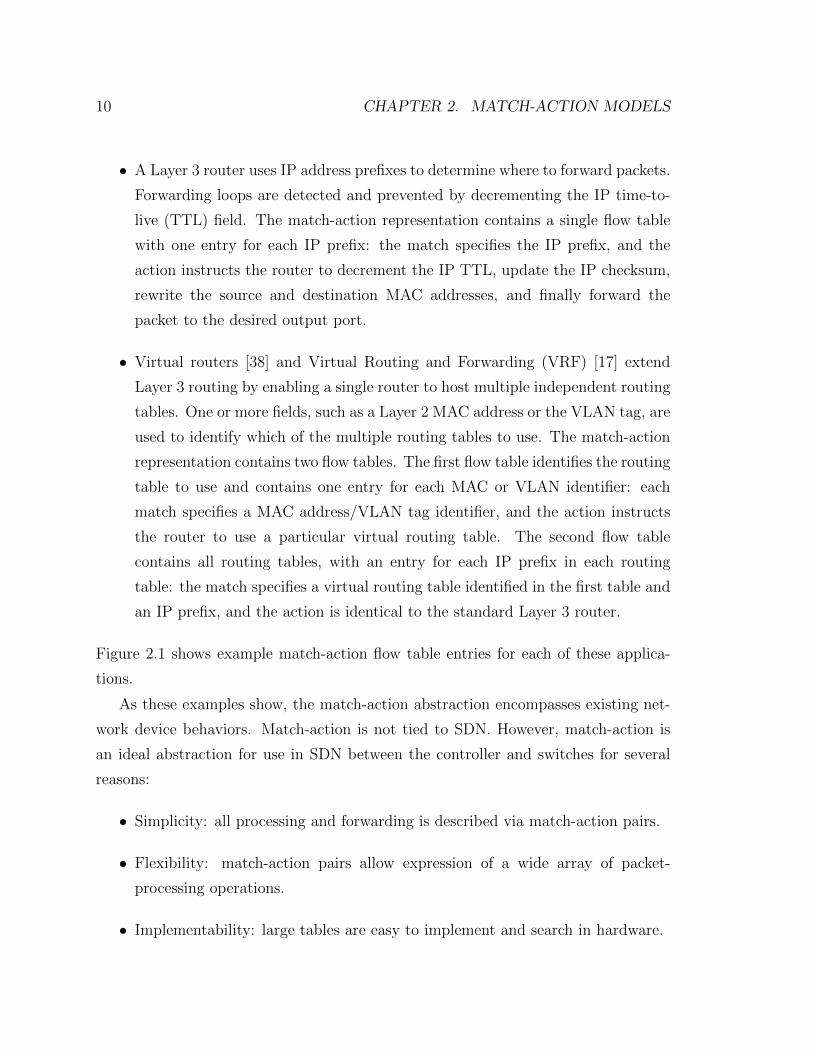
• A Layer 2 Ethernet switch uses Layer 2 MAC addresses to determine where
to forward packets to. The match-action representation contains a single flow
table with one entry for each host in the network: the match specifies the host’s
destination MAC address, and the action forwards the packet to the output
port that the host is connected to.
9
10 CHAPTER 2. MATCH-ACTION MODELS
• A Layer 3 router uses IP address prefixes to determine where to forward packets.
Forwarding loops are detected and prevented by decrementing the IP time-to-
live (TTL) field. The match-action representation contains a single flow table
with one entry for each IP prefix: the match specifies the IP prefix, and the
action instructs the router to decrement the IP TTL, update the IP checksum,
rewrite the source and destination MAC addresses, and finally forward the
packet to the desired output port.
• Virtual routers [38] and Virtual Routing and Forwarding (VRF) [17] extend
Layer 3 routing by enabling a single router to host multiple independent routing
tables. One or more fields, such as a Layer 2 MAC address or the VLAN tag, are
used to identify which of the multiple routing tables to use. The match-action
representation contains two flow tables. The first flow table identifies the routing
table to use and contains one entry for each MAC or VLAN identifier: each
match specifies a MAC address/VLAN tag identifier, and the action instructs
the router to use a particular virtual routing table. The second flow table
contains all routing tables, with an entry for each IP prefix in each routing
table: the match specifies a virtual routing table identified in the first table and
an IP prefix, and the action is identical to the standard Layer 3 router.
Figure 2.1 shows example match-action flow table entries for each of these applica-
tions.
As these examples show, the match-action abstraction encompasses existing net-
work device behaviors. Match-action is not tied to SDN. However, match-action is
an ideal abstraction for use in SDN between the controller and switches for several
reasons:
• Simplicity: all processing and forwarding is described via match-action pairs.
• Flexibility: match-action pairs allow expression of a wide array of packet-
processing operations.
• Implementability: large tables are easy to implement and search in hardware.
11
eth_
da =
00:
18:8
b:27
:bb:
01ou
tput
= 1
eth_
da =
00:
d0:0
5:5d
:24:
0aou
tput
= 2
Match
Action
(a)
Lay
er2
Eth
ern
etsw
itch
.
ip d
st =
192
.168
.0.0
/24
set m
ac d
st =
00:
1a:9
2:b8
:dc:
24,
set m
ac s
rc =
00:
d0:0
5:5d
:24:
0b,
dec
ttl, u
pdat
e ip
chk
sum
, out
put =
2
ip d
st =
0.0
.0.0
/0se
t mac
dst
= 0
0:1f
:bc:
09:1
a:60
,se
t mac
src
= 0
0:d0
:05:
5d:2
4:0d
,de
c ttl
, upd
ate
ip c
hksu
m, o
utpu
t = 4
Match
Action
(b)
Lay
er3
rou
ter.
vlan
= 1
set r
oute
tbl =
1
vlan
= 4
7se
t rou
te tb
l = 2
Match
Action
Tabl
e 1:
VLA
N →
rout
ing
tabl
e
rout
e tb
l = 1
,ip d
st =
192
.168
.1.1
/32
set m
ac d
st =
00:
18:8
b:27
:bb:
01,
set m
ac s
rc =
00:
d0:0
5:5d
:24:
0a,
dec
ttl, u
pdat
e ip
chk
sum
, out
put =
1
rout
e tb
l = 1
, ip
dst =
192
.168
.0.0
/24
set m
ac d
st =
00:
1a:9
2:b8
:dc:
24,
set m
ac s
rc =
00:
d0:0
5:5d
:24:
0b,
dec
ttl, u
pdat
e ip
chk
sum
, out
put =
2
rout
e tb
l = 2
, ip
dst =
192
.168
.0.0
/24
set m
ac d
st =
00:
1f:b
c:09
:1a:
60,
set m
ac s
rc =
00:
d0:0
5:5d
:24:
1d,
dec
ttl, u
pdat
e ip
chk
sum
, out
put =
4
rout
e tb
l = 2
, ip
dst =
0.0
.0.0
/0se
t mac
dst
= 0
0:b6
:d4:
89:b
3:19
,se
t mac
src
= 0
0:d0
:05:
5d:2
4:1b
,de
c ttl
, upd
ate
ip c
hksu
m, o
utpu
t = 2
Match
Action
Tabl
e 2:
Mul
tiple
rout
ing
tabl
es
(c)
Lay
er3
rou
ter
wit
hV
RF
.
Fig
ure
2.1:
Exam
ple
mat
ch-a
ctio
nflow
table
s.

12 CHAPTER 2. MATCH-ACTION MODELS
Match-action is easy to understand and facilitates the construction of low-cost, high-
performance implementations.
Discussion of the match-action abstraction has been mostly conceptual thus far. Nu-
merous match-action models can be created with differing properties. Design of any
match-action model is guided by a number of decisions, including:
• What’s the appropriate number of tables?
• How should packet data be treated and matches be expressed? Should the
packet be viewed as an opaque binary blob or as a sequence of headers and
fields?
• What’s an appropriate set of actions?
This chapter presents three match-action models: single match table (SMT), multiple
match tables (MMT), and reconfigurable match tables (RMT). SMT is powerful but
impractical; MMT overcomes SMT’s impracticalities but provides limited flexibility;
and RMT provides considerable flexibility. Many, including myself, believe that RMT
is the appropriate model for SDN going forward and, as Chapter 3 shows, RMT can
be implemented in hardware at a low cost.
2.1 Single Match Table
Single Match Table (SMT) is a simple yet powerful model. The model contains a
single flow table that matches against the first N bits of every packet. No semantic
meaning is associated with any of the bits by the switch. Each match is specified
as a (ternary) bit pattern, and actions are specified as bit manipulations. A binary
exact match is performed when all bits are fully specified, and a ternary match is
performed when some bits are “wildcarded” using a ternary “don’t care” or “X”
value. Figure 2.2 shows the SMT model.

2.1. SINGLE MATCH TABLE 13
Match Table
bits
Width: ∞
Dep
th: ∞
Packet
Figure 2.2: Single Match Table (SMT) model.
Superficially, the SMT abstraction is good for both programmers (what could be
simpler than a single match?) and implementers (SMT can be implemented using a
wide Ternary Content Addressable Memory or TCAM). Matching against the first N
bits of every packet makes the model protocol-agnostic: any protocol may be matched
by specifying the appropriate match bit sequence.
A closer look, however, shows that the SMT model is neither good for programmers
nor implementers because of several problems. First, control plane programmers
naturally think of packet bytes as a sequence of headers (e.g., Ethernet, IP) which
themselves are made from sequences of fields (e.g., IP destination, TTL).
Second, networks carry packets with a variety of encapsulation formats, and a
header might appear in several locations in different packets (e.g., IP-in-IP, IP over
MPLS, and IP-in-GRE). Mapping this to a flat SMT model requires programmers to
reason about all combinations of headers at all possible offsets at the bit level rather
than at the field level. The table must store entries for every offset where a header
appears.
Third, the use of a single table that matches the first N bits is inefficient. N
must be large enough to span all headers of interest, but this often results in many
wildcarded bits in entries, particularly when header behaviors are orthogonal. An
example of orthogonal behavior is performing Layer 2 Ethernet switching with some
entries and Layer 3 IP routing with other entries; the Layer 2 entries must wildcard
the Layer 3 fields and vice versa.
It can be even more wasteful if one header match affects another, for example,
if a match on the first header determines a disjoint set of values to match on the
14 CHAPTER 2. MATCH-ACTION MODELS
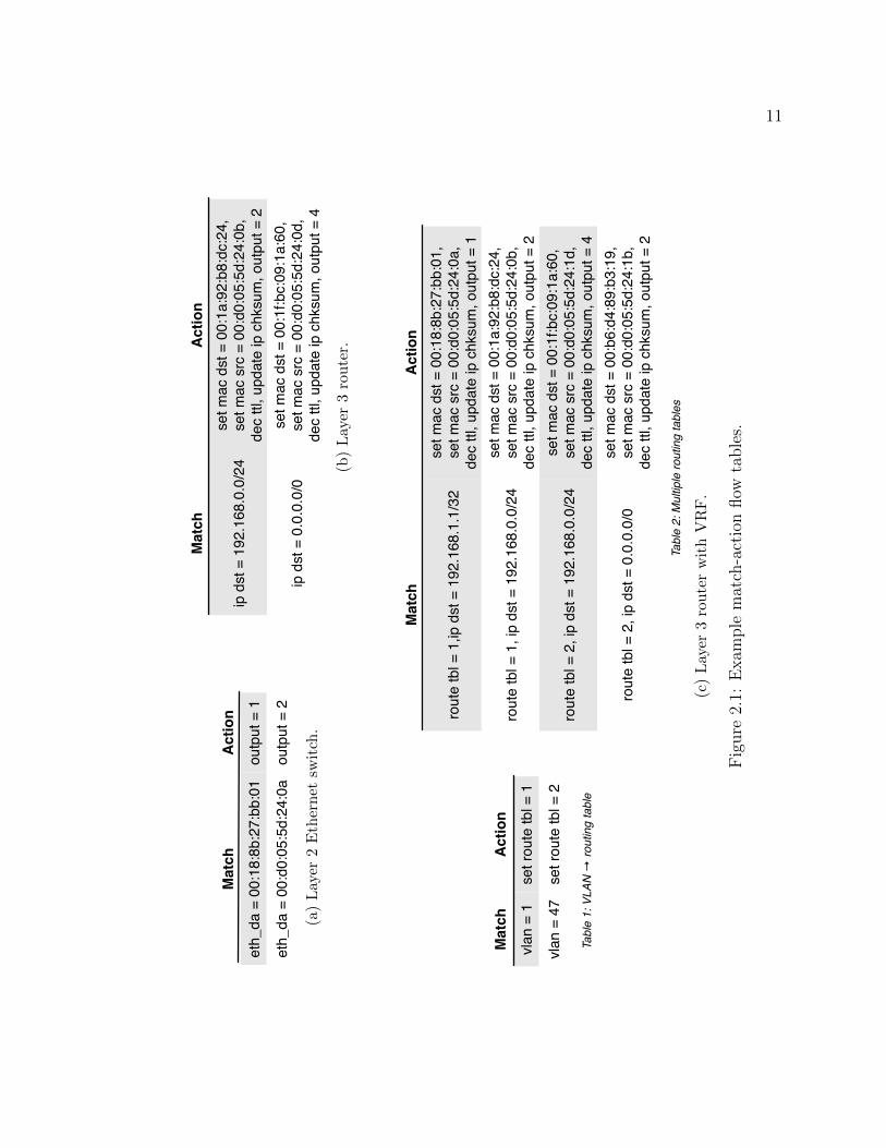
second header. In this scenario, the table must hold the Cartesian product of both
sets of headers. This behavior is seen in virtual routers, where the Ethernet MAC
address or VLAN tag determines the routing table to use for IP routing. If two tables
are used, then the first table contains the Ethernet MAC addresses or VLAN tags,
and the second contains the IP routing tables, as in Figure 2.3a. If one table is used,
each MAC/VLAN value must be paired with each entry from the appropriate routing
table, as in Figure 2.3b.
MAC 1 Route table: MAC 2
Match Action
Route table: MAC 3 Route table: MAC 4 Route table:
Route table: IP 1 …, Output = 1Route table: IP 2 …, Output = 2Route table: IP 3 …, Output = 3Route table: IP 1 …, Output = 4
Match Action
Route table: IP 2 …, Output = 5Route table: IP 3 …, Output = 6
(a) Virtual routing using two tables. The first table maps MAC addresses to routing tablesand the second table contains the routing tables. The tables contain a combined total of10 entries.
MAC 1, IP 1 …, Output = 1MAC 1, IP 2 …, Output = 2MAC 1, IP 3 …, Output = 3MAC 2, IP 1 …, Output = 1
Match Action
MAC 2, IP 2 …, Output = 2MAC 2, IP 3 …, Output = 3MAC 3, IP 1 …, Output = 4MAC 3, IP 2 …, Output = 5MAC 3, IP 3 …, Output = 6MAC 4, IP 1 …, Output = 4MAC 4, IP 2 …, Output = 5MAC 4, IP 3 …, Output = 6
(b) Virtual routing using one table. The table must contain the Cartesian product of allMAC address and routing table entries. The table contains 12 entries.
Figure 2.3: Example flow tables: virtual routing.(The red and blue regions represent independent routing tables.)

2.2. MULTIPLE MATCH TABLES 15
2.2 Multiple Match Tables
A natural refinement of the SMT model is the Multiple Match Tables (MMT) model.
MMT goes beyond SMT in two important ways: first, it raises the level of abstraction
from bits to fields (e.g., Ethernet destination address); second, it allows multiple
match tables that match on subsets of packet fields. Fields are extracted by a parser
and then routed to the appropriate match table. The match tables are arranged into
a pipeline of stages; stage i can modify data passed to and used in stage j > i, thereby
influencing j’s processing. Figure 2.4 shows the MMT model.
Match Table 1
fields
Width: W1
Dep
th: D
n
Packet
Parser
Match Table n
Width: Wn
fields
Dep
th: D
1
...
Figure 2.4: Multiple Match Table (MMT) model.
The MMT model eliminates the problems identified with the SMT model. Pro-
grammers can work at the intuitive level of fields instead of bits. Programmers no
longer need to reason about header combinations and their offsets as this is handled
by the parser. Narrower tables that match on specific headers can be used, and
orthogonal matches can be split across multiple tables to eliminate the Cartesian
product problem.
Existing switch chip pipelines may be viewed as realizations of the MMT model.
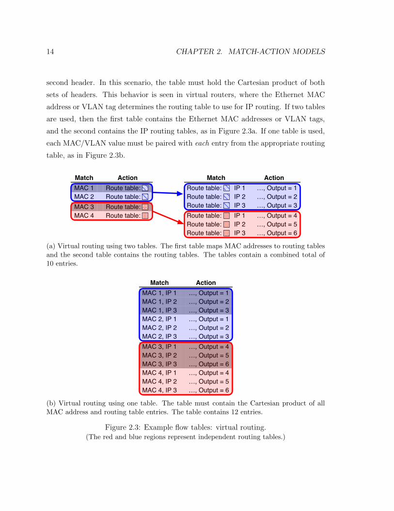
Figure 2.5 shows a pipeline representative of current chips.
An exploration of conventional pipelines reveals several shortcomings of the MMT
model. The first problem is that the number, widths, depths, and execution order
of tables in the pipeline is fixed. Existing switch chips (e.g., [7–9, 74, 75]) implement
16 CHAPTER 2. MATCH-ACTION MODELS
Parser
Match Tables
L2 Table
Ethernet Switching
L3 Table
IPRouting
L2–4 Table
Access Control List
ActionProcessing
Header fields
Packets
In
L2fields
L3fields
L2-4fields
Queues
Out
Figure 2.5: A conventional switch pipeline contains multiple tables that match ondifferent fields. A typical pipeline consists of an Ethernet switching table that matcheson L2 destination MAC addresses, an IP routing table that matches on IP addresses,and an Access Control List (ACL) table that matches any L2–L4 field. The parserbefore the pipeline identifies headers and extracts fields for use in the match tables.
a small number (4–8) of tables whose widths, depths, and execution order are set
when the chip is fabricated. A chip used for an L2 bridge may want to have a 48-
bit destination MAC address match table and a second 48-bit source MAC address
learning table; a chip used for a core router may require a very large 32-bit IP longest
prefix match table and a small 128-bit ACL match table; an enterprise router may
want to have a smaller 32-bit IP prefix table, a much larger ACL table, and some MAC
address match tables. Fabricating separate chips for each use case is inefficient, and
so merchant switch chips tend to be designed to support the superset of all common
configurations, with a set of fixed size tables arranged in a predetermined pipeline
order. This creates a problem for network owners who want to tune the table sizes
to optimize for their network, or implement new forwarding behaviors beyond those
defined by existing standards. In practice, MMT translates to fixed multiple match
tables.
A second subtler problem is that switch chips offer only a limited repertoire of
actions corresponding to common processing behaviors, e.g., forwarding, dropping,
decrementing TTLs, pushing VLAN or MPLS headers, and GRE encapsulation. This
action set is not easily extensible, and also not very abstract. A more abstract set of
actions should allow any field to be modified, any state machine associated with the
2.3. RECONFIGURABLE MATCH TABLES 17
packet to be updated, and the packet to be forwarded to an arbitrary set of output
ports.
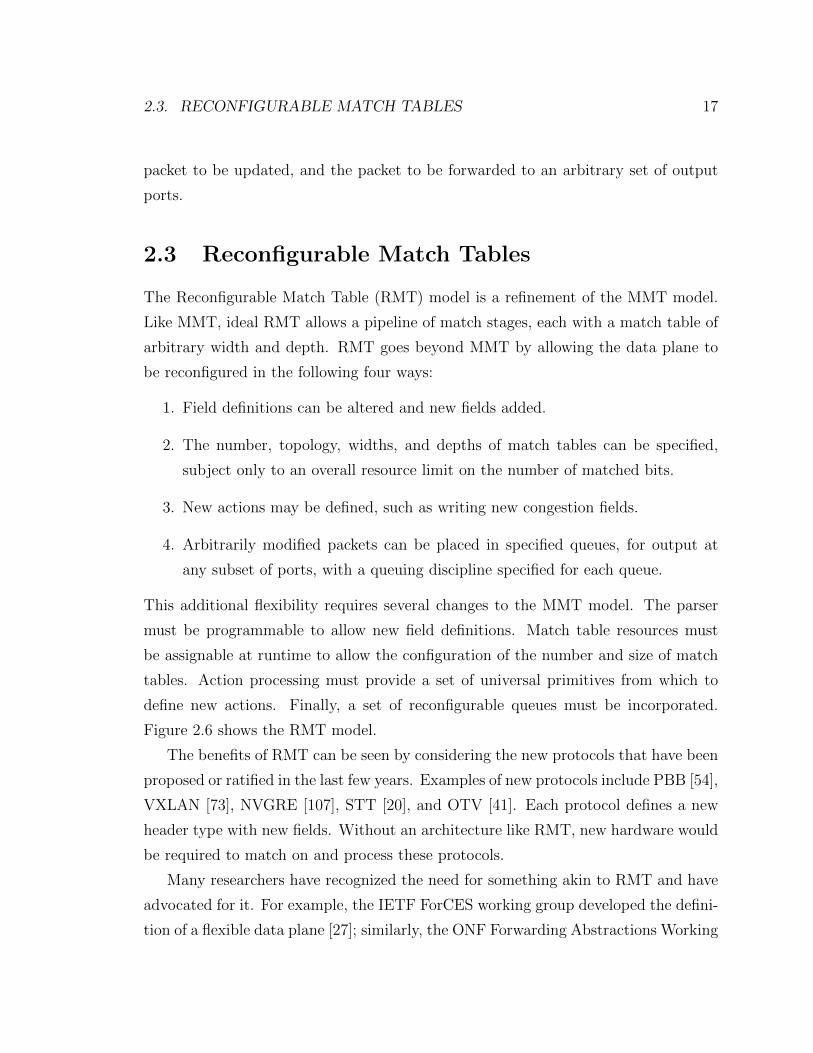
2.3 Reconfigurable Match Tables
The Reconfigurable Match Table (RMT) model is a refinement of the MMT model.
Like MMT, ideal RMT allows a pipeline of match stages, each with a match table of
arbitrary width and depth. RMT goes beyond MMT by allowing the data plane to
be reconfigured in the following four ways:
1. Field definitions can be altered and new fields added.
2. The number, topology, widths, and depths of match tables can be specified,
subject only to an overall resource limit on the number of matched bits.
3. New actions may be defined, such as writing new congestion fields.
4. Arbitrarily modified packets can be placed in specified queues, for output at
any subset of ports, with a queuing discipline specified for each queue.
This additional flexibility requires several changes to the MMT model. The parser
must be programmable to allow new field definitions. Match table resources must
be assignable at runtime to allow the configuration of the number and size of match
tables. Action processing must provide a set of universal primitives from which to
define new actions. Finally, a set of reconfigurable queues must be incorporated.
Figure 2.6 shows the RMT model.
The benefits of RMT can be seen by considering the new protocols that have been
proposed or ratified in the last few years. Examples of new protocols include PBB [54],
VXLAN [73], NVGRE [107], STT [20], and OTV [41]. Each protocol defines a new
header type with new fields. Without an architecture like RMT, new hardware would
be required to match on and process these protocols.
Many researchers have recognized the need for something akin to RMT and have
advocated for it. For example, the IETF ForCES working group developed the defini-
tion of a flexible data plane [27]; similarly, the ONF Forwarding Abstractions Working

18 CHAPTER 2. MATCH-ACTION MODELS
Match Table 1
fields
Width: W1
Dep
th: D
n
Packet
Parser
Match Table n
Width: Wn
fields
Dep
th: D
1
...
Reconfigurable
Figure 2.6: Reconfigurable Match Table (RMT) model.
Group has worked on reconfigurability [89]. However, there has been understandable
skepticism that the RMT model is implementable at very high speeds. Without a
chip to provide an existence proof of RMT, it has seemed fruitless to standardize the
reconfiguration interface between the controller and the data plane.
2.4 Match-action models and OpenFlow
OpenFlow has always used the match-action abstraction to specify flow entries. Open-
Flow 1.0 [90] uses a single table version of MMT: the switch is modelled as a single
flow table that matches on fields. OpenFlow 1.1 [91] transitioned to a multiple table
version of MMT, which has remained the status quo [92–94]. The specification does
not mandate the width, depth, or even the number of tables, leaving implementors
free to choose their multiple tables. A number of fields (e.g., Ethernet and IP fields)
and actions (e.g., set field and goto table) have been standardized in the specification;
these may be a subset of the fields and actions supported by the switch. A facility
exists to allow switch vendors to introduce new fields and actions, but the specifica-
tion does not allow the controller to define these. The similarity between the MMT
model and merchant silicon designs make it possible to map OpenFlow onto existing
pipelines [10, 48, 55, 86]. Google reports converting their entire private WAN to this
approach using merchant switch chips [49].
2.4. MATCH-ACTION MODELS AND OPENFLOW 19
RMT, as a superset of MMT, is perfectly compatible with (and even partly imple-
mented by) the current OpenFlow specification. The ONF Forwarding Abstractions
Working Group recognizes the need for reconfigurability and is attempting to enable
“pre-runtime” configuration of switch tables. Some existing chips, driven at least in
part by the need to address multiple market segments, already have some flavors of
reconfigurability that can be expressed using ad hoc interfaces to the chip.

20 CHAPTER 2. MATCH-ACTION MODELS
Chapter 3
Hardware design for Match-Action
SDN
Match-action is an ideal abstraction for SDN: it is conceptually simple; it provides
the power to express most in-network packet processing; and its flow table driven
structure makes certain flavors readily amenable to hardware implementation. In
fact, as §2.2 shows, current switch chip architectures match the MMT model, allowing
OpenFlow to be implemented on many of them.
Although many OpenFlow switches are available on the market today, they fail
to live up to the full promise of SDN due to the shortcomings identified in Chapter 1.
Many of these shortcomings relate to a lack of flexibility, particularly the inability
to specify the number, size, and arrangement of tables; the inability to define new
headers; and the inability to define new actions. The RMT model addresses this
lack of flexibility by explicitly enabling configuration in each of these dimensions.
However, the question remains as to whether an RMT implementation is practical at
a reasonable cost without sacrificing speed.
One can imagine implementing RMT in software on a general purpose CPU. But
for the speeds of modern switches—about 1 Tb/s today [9, 74]—we need the paral-
lelism of dedicated hardware. Switch chips are two orders of magnitude faster at
switching than CPUs [26], and an order of magnitude faster than network proces-
sors [16, 34, 43, 87]; this has been true for over a decade and the trend is unlikely to
21
22 CHAPTER 3. HARDWARE DESIGN FOR MATCH-ACTION SDN
change. We therefore need to think through how to implement RMT in hardware to
exploit pipelining and parallelism while living within the constraints of on-chip table
memories.
Intuitively, arbitrary reconfigurability at terabit speeds seems an impossible mis-
sion. Fortunately, arbitrary reconfigurability it not required. A design with a re-
stricted degree of flexibility is useful if it covers a sufficiently large fraction of needs.
The challenge is providing sufficient flexibility while operating at terabit speeds while
remaining cost-competitive with fixed-table MMT chips. This chapter shows that
highly flexible RMT hardware can be built at a cost less than 15% above that of
equivalent conventional switch hardware.
General purpose payload processing is not the goal. The design aims to identify
the essential minimal set of primitives to process headers in hardware. RMT actions
can be thought of as a minimal instruction set like RISC, designed to run really fast
in heavily pipelined hardware.
The chapter is structured as follows. It begins by considering the feasibility of
implementing RMT using existing switch chips. It then proposes an architecture to
implement the RMT model and provides configuration examples that show how to
use the proposed RMT architecture to implement several use cases. The chapter then
explains the design in detail and evaluates the chip design and cost before concluding
with a comparison to existing work.
3.1 RMT and traditional switch ASICs
Merchant silicon vendors, such as Broadcom, Marvell, and Intel, manufacture the
switch ASICs found within many enterprise wiring closet and data center top-of-rack
(ToR) switches. These devices are available in capacities ranging from gigabits to
terabits [7–9, 74, 75]. Common among these chips is a basic high-level architecture:
they contain a parser that identifies and extracts fields from received packets, multiple
match tables that match extracted fields to determine the actions to apply, logic to
apply the desired actions, and buffer memory to store packets prior to transmission.
The set of supported headers—and the number, type, and arrangement of match
3.1. RMT AND TRADITIONAL SWITCH ASICS 23
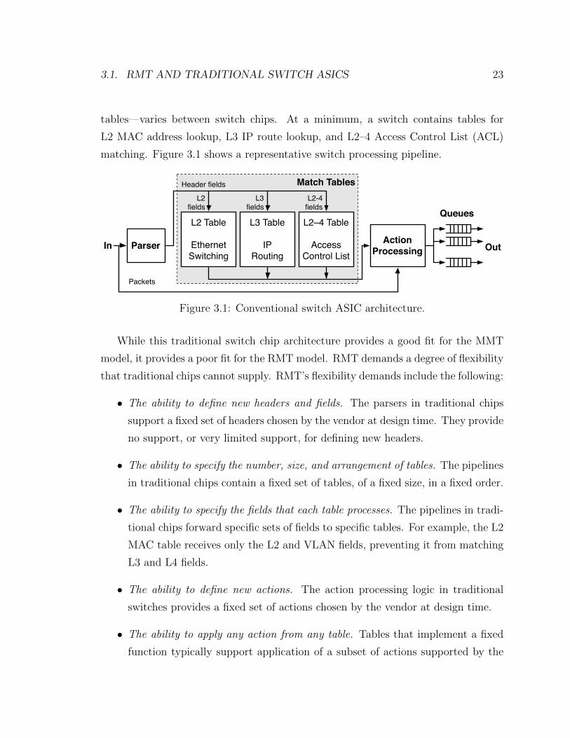
tables—varies between switch chips. At a minimum, a switch contains tables for
L2 MAC address lookup, L3 IP route lookup, and L2–4 Access Control List (ACL)
matching. Figure 3.1 shows a representative switch processing pipeline.
Parser
Match Tables
L2 Table
Ethernet Switching
L3 Table
IPRouting
L2–4 Table
Access Control List
ActionProcessing
Header fields
Packets
In
L2fields
L3fields
L2-4fields
Queues
Out
Figure 3.1: Conventional switch ASIC architecture.
While this traditional switch chip architecture provides a good fit for the MMT
model, it provides a poor fit for the RMT model. RMT demands a degree of flexibility
that traditional chips cannot supply. RMT’s flexibility demands include the following:
• The ability to define new headers and fields. The parsers in traditional chips
support a fixed set of headers chosen by the vendor at design time. They provide
no support, or very limited support, for defining new headers.
• The ability to specify the number, size, and arrangement of tables. The pipelines
in traditional chips contain a fixed set of tables, of a fixed size, in a fixed order.
• The ability to specify the fields that each table processes. The pipelines in tradi-
tional chips forward specific sets of fields to specific tables. For example, the L2
MAC table receives only the L2 and VLAN fields, preventing it from matching
L3 and L4 fields.
• The ability to define new actions. The action processing logic in traditional
switches provides a fixed set of actions chosen by the vendor at design time.
• The ability to apply any action from any table. Tables that implement a fixed
function typically support application of a subset of actions supported by the
24 CHAPTER 3. HARDWARE DESIGN FOR MATCH-ACTION SDN
chip. For example, the L2 MAC table only provides the ability to forward a
packet to one or more ports and, possibly, to modify the VLAN tag.
Good support for RMT requires a new design for switch ASICs. The remainder of
this chapter describes such a design.
3.2 RMT architecture
The RMT model definition in §2.3 states that RMT allows a pipeline of match stages,
each with a match table of arbitrary width and depth, that match on arbitrary fields.
A logical deduction is that an RMT switch consists of a parser, to enable matching
on fields, followed by an arbitrary number of match stages. Prudence suggests the
inclusion of queuing to handle congestion at the outputs. Figure 3.2a presents a
logical architecture for the RMT model.
Looking a little deeper, the parser identifies headers and extracts fields. The RMT
model dictates that it be possible to modify or add field definitions, requiring that
the parser be reconfigurable. The parser output is a packet header vector, which is
a set of header fields such as IP destination address, Ethernet destination MAC, and
so on. The packet header vector also includes “metadata” fields; these include the
input port on which the packet arrived and other router state variables, such as the
current size of router queues.
The header vector flows through a sequence of logical match stages, each of which
abstracts a logical unit of packet processing (e.g., Ethernet or IP processing). The
match table size is configurable within each logical match stage. For example, one
might want a match table of 256 K × 32-bit prefixes for IP routing, or a match table
of 64 K × 48-bit addresses for L2 Ethernet forwarding. Each match stage may use
any of the fields within the packet header vector as inputs. An input selector within
each logical stage extracts the fields to be matched from the header vector.
Packet modifications are performed by the VLIW Action block. A Very Long
Instruction Word (VLIW) specifies the actions to apply to each field, and these actions
are applied in parallel to the vector. More precisely, an action unit exists for each field
F in the header vector, as Figure 3.2c shows. Each action unit takes up to three input

3.2. RMT ARCHITECTURE 25
Confi
gura
ble
Out
put
Que
ues
Prog
. Pa
rser
Switc
h St
ate
(met
adat
a)
Recombine
Pack
ets
Out
put
Chan
nels
Pack
ets
Inpu
t Ch
anne
ls
Logi
cal S
tage
1Lo
gica
l Sta
ge N
1 K
1 K
�
�
�…
New Header
Header Payload
…Select
VLIW
Actio
nM
atch
Ta
bles
Stat
istics
Stat
e
…
(a)
RM
Tm
od
elas
ase
qu
ence
oflo
gica
lM
atch
-Act
ion
stag
es.
Logi
cal S
tage
1
Logi
cal S
tage
2
Logi
cal
Stag
e N
Phys
ical
St
age
1Ph
ysic
alSt
age
2Ph
ysic
al
Stag
e M
Ingr
ess
logi
cal
mat
ch ta
bles
Egre
ss lo
gica
lm
atch
tabl
es
…
(b)
Fle
xib
lem
atch
tab
leco
nfi
gura
tion
.
Pack
et
Hea
der
Vect
or
Pack
et
Hea
der
Vect
or
Action Input Selector (Crossbar)
Actio
n M
emor
y
VLIW
Inst
ruct
ion
Mem
ory
Very WideHeader Bus
…
ActionUnit
ActionUnit
Mat
chTa
bles
Mat
chRe
sults
…
OP
code
(from
inst
mem
)
OP
code
CtrlSr
c 1
Src
2
Src
3
Src
1
Src
2
Src
3
(c)
VL
IWac
tion
arc
hit
ectu
re.
Fig
ure
3.2:
RM
Tm
odel
arch
itec
ture
.

26 CHAPTER 3. HARDWARE DESIGN FOR MATCH-ACTION SDN
values (including fields from the header vector and action data results corresponding
with the match) and rewrites F . Instructions also allow limited state (e.g., counters)
to be modified, which may influence the processing of subsequent packets.
Allowing each logical stage to rewrite every field may appear to be overkill, but
it allows shifting headers. For example, a logical MPLS stage may pop an MPLS
header, shifting subsequent MPLS headers forward, while a logical IP stage may
simply decrement the TTL. The cost of including an action unit per field is small
compared with the cost of the match tables, as §3.5 shows.
A next-table address output from each table match determines control flow; this
next-table address specifies the logical table to execute next. For example, a match on
a specific Ethertype in Stage 1 could direct processing to a later stage that performs
prefix matching on IP addresses (routing), while a different Ethertype could direct
processing to a different stage that performs exact matching on Ethernet addresses
(bridging).
The match stages control each packet’s fate by updating a set of destination ports
and queues. A stage sets a single destination port to unicast a packet, sets multiple
destination ports to multicast a packet, and clears the destination ports to drop a
packet. A stage applies QoS mechanisms, such as token bucket, by specifying an
output queue that has been preconfigured to use the desired mechanism.
The recombination block at the end of the pipeline “pushes” header vector modi-
fications back into the packet. Finally, the packet is placed in the specified queues at
the specified output ports, and a configurable queuing discipline is applied.
In summary, the RMT logical architecture of Figure 3.2a allows new fields to be
added by modifying the parser, new fields to be matched by modifying match memo-
ries, new actions to be applied by modifying stage instructions, and new queueing by
modifying the queueing discipline for each queue. The RMT logical architecture can
simulate existing devices, such as a bridge, a router, or a firewall; implement existing
protocols, such as MPLS and ECN; and implement new protocols proposed in the
literature—such as RCP [30]—that use non-standard congestion fields. Most impor-
tantly, the RMT logical architecture allows future data plane modifications without
requiring hardware modifications.
3.2. RMT ARCHITECTURE 27
3.2.1 Implementation architecture at 640 Gb/s
The proposed implementation architecture for the RMT model maps a small set of
logical match stages to a larger number of physical match stages. The mapping of
logical to physical stages is determined by the resource needs of each logical stage.
Multiple logical match stages that require few resources can share the same physical
stage, while a logical match stage that requires many resources can use multiple
physical stages. Figure 3.2b shows this architecture. The implementation architecture
is motivated by the following:
1. Factoring State: Switch forwarding typically has several stages (e.g., routing,
ACL), each of which uses a separate table; combining these into one table
produces the Cartesian product of states. Stages are processed sequentially
with dependencies, so a physical pipeline is natural.
2. Flexible Resource Allocation Minimizing Resource Waste: A physical match
stage has a fixed set of resources (e.g., CPU, memory). The resources needed for
a logical match stage can vary considerably. For example, a firewall may require
all ACLs; a core router may require only prefix matches; and an edge router
may require some of each. By flexibly allocating logical stages onto physical
stages, one can reconfigure the pipeline to metamorphose from a firewall to
a core router in the field. The number of physical stages N should be large
enough so that a logical stage that uses few resource will waste at most 1/Nth of
the resources. Of course, increasing N increases overhead (e.g., wiring, power);
N = 32 was chosen in this design as a compromise between reducing resource
wastage and hardware overhead.
3. Layout Optimality: A logical stage may be assigned more memory than that
contained in a single physical stage by assigning the logical stage to multiple
contiguous physical stages, as shown in Figure 3.2b. The configuration process
splits the logical stage into subsections that it assigns to consecutive physical
stages. The implementation performs lookups in all subsections but applies
only the actions corresponding to the first matching entry. An alternate design

28 CHAPTER 3. HARDWARE DESIGN FOR MATCH-ACTION SDN
is to assign each logical stage to a decoupled set of memories via a crossbar [13].
While this design is more flexible—any memory bank can be allocated to any
stage—the worst-case wire delays between a processing stage and memories
grow at a rate of√M or more, which, in chips that require a large amount of
memory M , can be large. These delays can be ameliorated by pipelining, but
the ultimate challenge in such a design is wiring: unless the current match and
action widths (1280 bits) are reduced, running so many wires between every
stage and every memory may well be impossible.
In sum, the advantage of the architecture in Figure 3.2b is that it uses a tiled structure
with short wires whose resources can be reconfigured with minimal waste. Two dis-
advantages of this approach should be noted. First, power requirements are inflated
by the use of more physical stages than necessary. Second, this implementation archi-
tecture conflates processing and memory allocation. A logical stage requiring more
processing must be allocated two physical stages, but this allocates twice the memory
even though the stage may not need it. In practice, neither issue is significant: the
power used by the stage processors is at most 10% of the total power usage within
the chip design, and most use cases in networking are dominated by memory use, not
processing.
3.2.2 Restrictions for realizability
A number of restrictions must be imposed to enable realization of the physical match
stage architecture at terabit-speed:
Match restrictions:
The design must contain a fixed number of physical match stages with a fixed
set of resources. The proposed design provides 32 physical match stages at
both ingress and egress. Match-action processing at egress allows more efficient
processing of multicast packets by deferring per-port modifications until after
buffering.
Packet header limits:
A width must be selected for the packet header vector used for matching and
3.2. RMT ARCHITECTURE 29
action processing. The proposed design contains a 4 Kb (512 B) vector, which
allows processing complex headers and sequences of headers.
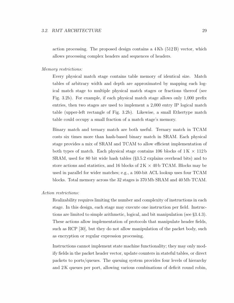
Memory restrictions:
Every physical match stage contains table memory of identical size. Match
tables of arbitrary width and depth are approximated by mapping each log-
ical match stage to multiple physical match stages or fractions thereof (see
Fig. 3.2b). For example, if each physical match stage allows only 1,000 prefix
entries, then two stages are used to implement a 2,000 entry IP logical match
table (upper-left rectangle of Fig. 3.2b). Likewise, a small Ethertype match
table could occupy a small fraction of a match stage’s memory.
Binary match and ternary match are both useful. Ternary match in TCAM
costs six times more than hash-based binary match in SRAM. Each physical
stage provides a mix of SRAM and TCAM to allow efficient implementation of
both types of match. Each physical stage contains 106 blocks of 1 K × 112 b
SRAM, used for 80 bit wide hash tables (§3.5.2 explains overhead bits) and to
store actions and statistics, and 16 blocks of 2 K × 40 b TCAM. Blocks may be
used in parallel for wider matches; e.g., a 160-bit ACL lookup uses four TCAM
blocks. Total memory across the 32 stages is 370 Mb SRAM and 40 Mb TCAM.
Action restrictions:
Realizability requires limiting the number and complexity of instructions in each
stage. In this design, each stage may execute one instruction per field. Instruc-
tions are limited to simple arithmetic, logical, and bit manipulation (see §3.4.3).
These actions allow implementation of protocols that manipulate header fields,
such as RCP [30], but they do not allow manipulation of the packet body, such
as encryption or regular expression processing.
Instructions cannot implement state machine functionality; they may only mod-
ify fields in the packet header vector, update counters in stateful tables, or direct
packets to ports/queues. The queuing system provides four levels of hierarchy
and 2 K queues per port, allowing various combinations of deficit round robin,
30 CHAPTER 3. HARDWARE DESIGN FOR MATCH-ACTION SDN
hierarchical fair queuing, token buckets, and priorities. However, it cannot sim-
ulate the sorting required for weighted fair queueing (WFQ) for example.
In this design, each stage contains over 200 action units: one for each field in
the packet header vector. Over 7,000 action units are contained in the chip,
but these consume a small area in comparison to memory (< 10%). The action
unit processors are simple, specifically architected to avoid costly to implement
instructions, and require less than 100 gates per bit.
Configuration of the RMT architecture requires two pieces of information: a parse
graph that expresses permissible header sequences and a table flow graph that ex-
presses the set of match tables and the control flow between them. §3.3 provides
examples of parse graphs and table flow graphs, and §4.2 and §3.4.4 explain each in
more detail. Compilers should perform the mapping from these graphs to the appro-
priate switch configuration. Chapter 4 provides details on compiling parse graphs;
compilation of table flow graphs is outside the scope of this dissertation.
3.3 Example use cases
This section provides several example use cases that illustrate the usage of the RMT
model and proposed RMT switch design. The chosen examples are connected and
build upon one another: the first implements a hybrid L2/L3 switch; the second adds
support for ACLs and RCP; and the third adds processing of a custom protocol.
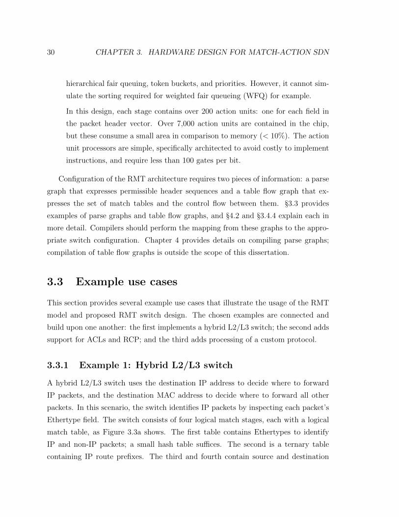
3.3.1 Example 1: Hybrid L2/L3 switch
A hybrid L2/L3 switch uses the destination IP address to decide where to forward
IP packets, and the destination MAC address to decide where to forward all other
packets. In this scenario, the switch identifies IP packets by inspecting each packet’s
Ethertype field. The switch consists of four logical match stages, each with a logical
match table, as Figure 3.3a shows. The first table contains Ethertypes to identify
IP and non-IP packets; a small hash table suffices. The second is a ternary table
containing IP route prefixes. The third and fourth contain source and destination

3.3. EXAMPLE USE CASES 31
MAC addresses for learning and forwarding, respectively, implemented as hash tables.
The IP route and the two MAC tables should be as large as possible to maximize the
number of addresses they can store.
Ethertype
IPv4 routing Src MAC Dst MAC
IP packets Non-IP packets
(a) Logical tables.
IPv4
Ethernet
END
END
(b) Parse graph.
IP route
Ethertype
Src MAC Dst MACAction: Setsrc/dst MAC,
decrement IP TTL
Action: Sendto controller
Action: Setoutput port
(c) Flow graph.1 2 32…Stage:
TCAM
RAM
(d) Memory allocation.
Legend
{Ethertype}{Dst IP}{Src Port, Src MAC}{Dst MAC}
Table FieldsLogical flow
Drop packetForward to buffer
Table Flow Graph
Figure 3.3: Hybrid L2/L3 switch configuration.
A parse graph specifies the headers within a network and their permitted ordering.
As Figure 3.3b shows, the switch processes Ethernet and IPv4 headers only; packets
always begin with an Ethernet header, and the IPv4 header is optional. A compiler
translates the parse graph into the parser configuration. This configuration instructs
the parser to extract and place five fields in the packet header vector: Ethernet Des-
tination MAC Address (L2 DA), Ethernet Source MAC Address (L2 SA), Ethertype,
IP Destination Address (IP DA), and IP TTL. Chapter 4 provides more detail on
parse graphs and their compilation.
The table flow graph (Figure 3.3c) specifies the match tables, the fields that each
match tables uses from the header vector, and the dependencies between tables. Using
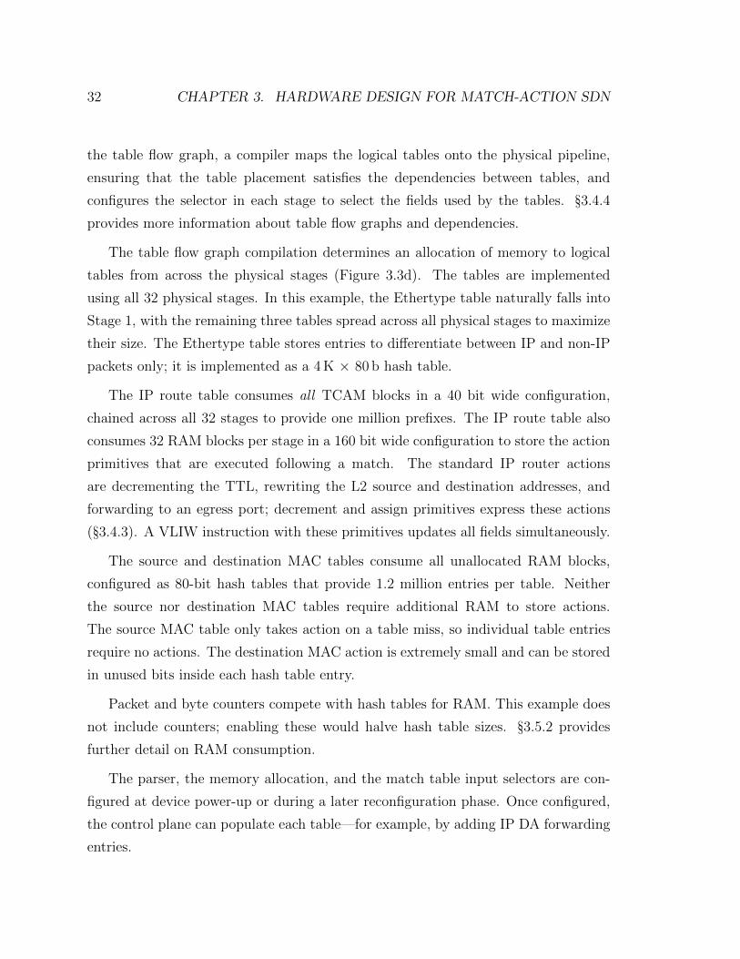
32 CHAPTER 3. HARDWARE DESIGN FOR MATCH-ACTION SDN
the table flow graph, a compiler maps the logical tables onto the physical pipeline,
ensuring that the table placement satisfies the dependencies between tables, and
configures the selector in each stage to select the fields used by the tables. §3.4.4
provides more information about table flow graphs and dependencies.
The table flow graph compilation determines an allocation of memory to logical
tables from across the physical stages (Figure 3.3d). The tables are implemented
using all 32 physical stages. In this example, the Ethertype table naturally falls into
Stage 1, with the remaining three tables spread across all physical stages to maximize
their size. The Ethertype table stores entries to differentiate between IP and non-IP
packets only; it is implemented as a 4 K × 80 b hash table.
The IP route table consumes all TCAM blocks in a 40 bit wide configuration,
chained across all 32 stages to provide one million prefixes. The IP route table also
consumes 32 RAM blocks per stage in a 160 bit wide configuration to store the action
primitives that are executed following a match. The standard IP router actions
are decrementing the TTL, rewriting the L2 source and destination addresses, and
forwarding to an egress port; decrement and assign primitives express these actions
(§3.4.3). A VLIW instruction with these primitives updates all fields simultaneously.
The source and destination MAC tables consume all unallocated RAM blocks,
configured as 80-bit hash tables that provide 1.2 million entries per table. Neither
the source nor destination MAC tables require additional RAM to store actions.
The source MAC table only takes action on a table miss, so individual table entries
require no actions. The destination MAC action is extremely small and can be stored
in unused bits inside each hash table entry.
Packet and byte counters compete with hash tables for RAM. This example does
not include counters; enabling these would halve hash table sizes. §3.5.2 provides
further detail on RAM consumption.
The parser, the memory allocation, and the match table input selectors are con-
figured at device power-up or during a later reconfiguration phase. Once configured,
the control plane can populate each table—for example, by adding IP DA forwarding
entries.

3.3. EXAMPLE USE CASES 33
Lookup and processing within the 32 match stages occurs as shown in Figure 3.4.
For simplicity, processing within a stage is partitioned into match and action phases;
the match phase requires m cycles, and the action phase requires a cycles. The
packet header vector is partitioned into input fields and output fields, which travel
independently through the pipeline.
Match Action
Stage 1
Stage 2
Stage 3
Time
⋮ ⋮⋮
0 1 2 3 4 5 6 7 8 9
EthertypeIP routeSrc MACDst MAC
EthertypeIP routeSrc MACDst MAC
I OS
Match ActionIP routeSrc MACDst MAC
IP routeSrc MACDst MAC
I OS
m a
Ethertype match identifies IP route as the next table
No match in Stage 1 IP route table. Apply actions in Stage 2.
Match ActionIP routeSrc MACDst MAC
IP routeSrc MACDst MAC
I OS
Successful match in Stage 2 IP route table. Do NOT apply actions in Stage 3.
: Input fields
: Match status
: Output fields
I
O
S
Figure 3.4: Hybrid L2/L3 switch match stage processing.
The input fields arrive at Stage 1 at time t = 0. Stage 1 contains the Ethertype
table and subsections of the IP route, Ethernet source MAC, and Ethernet destination
MAC tables. Successor dependencies exist between the Ethertype table and each of
the other tables. Matching commences in all four tables at t = 0 and complete at
t = m. Action processing commences immediately after completion of the matches.
The result of the Ethertype table match indicates the other tables that should process
the packet; action processing is only applied for the indicated table(s). Stage 1
completes action processing and emits the output fields at t = l + a.
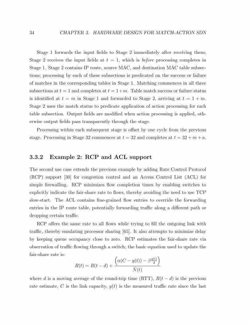
34 CHAPTER 3. HARDWARE DESIGN FOR MATCH-ACTION SDN
Stage 1 forwards the input fields to Stage 2 immediately after receiving them;
Stage 2 receives the input fields at t = 1, which is before processing completes in
Stage 1. Stage 2 contains IP route, source MAC, and destination MAC table subsec-
tions; processing by each of these subsections is predicated on the success or failure
of matches in the corresponding tables in Stage 1. Matching commences in all three
subsections at t = 1 and completes at t = 1+m. Table match success or failure status
is identified at t = m in Stage 1 and forwarded to Stage 2, arriving at t = 1 + m.
Stage 2 uses the match status to predicate application of action processing for each
table subsection. Output fields are modified when action processing is applied, oth-
erwise output fields pass transparently through the stage.
Processing within each subsequent stage is offset by one cycle from the previous
stage. Processing in Stage 32 commences at t = 32 and completes at t = 32 +m+ a.
3.3.2 Example 2: RCP and ACL support
The second use case extends the previous example by adding Rate Control Protocol
(RCP) support [30] for congestion control and an Access Control List (ACL) for
simple firewalling. RCP minimizes flow completion times by enabling switches to
explicitly indicate the fair-share rate to flows, thereby avoiding the need to use TCP
slow-start. The ACL contains fine-grained flow entries to override the forwarding
entries in the IP route table, potentially forwarding traffic along a different path or
dropping certain traffic.
RCP offers the same rate to all flows while trying to fill the outgoing link with
traffic, thereby emulating processor sharing [65]. It also attempts to minimize delay
by keeping queue occupancy close to zero. RCP estimates the fair-share rate via
observation of traffic flowing through a switch; the basic equation used to update the
fair-share rate is:
R(t) = R(t− d) +
(α(C − y(t))− β q(t)
d
)N(t)
where d is a moving average of the round-trip time (RTT), R(t − d) is the previous
rate estimate, C is the link capacity, y(t) is the measured traffic rate since the last

3.3. EXAMPLE USE CASES 35
rate update, q(t) is the instantaneous queue size, N(t) is the estimate of the number
of ongoing flows, and α and β are parameters chosen for stability and performance.
The update equation shares excess capacity (i.e., C−y(t) > 0) equally amongst all
flows, and penalizes all flows equally when a link is oversubscribed (i.e., C−y(t) < 0).
The rate is decreased when the queue builds up; q(t)d
is the bandwidth needed to drain
the queue within an RTT.
RCP support requires the switch to perform additional processing on packet
ingress and egress. Ingress processing updates several counters that are used to mea-
sure the traffic arrival rate and to update the RTT moving average; Algorithm 1
describes this processing. Egress processing stamps the calculated fair-share rate
into the RCP header; Algorithm 2 describes this processing. Only integer arith-
metic is required for the ingress and egress processing, making it readily amenable
to implementation in hardware. The periodic fair-share rate update calculations are
performed in the control plane.
Algorithm 1 RCP packet-arrival processing.
input traffic bytes ← input traffic bytes + packet size bytesif this packet RTT < MAX ALLOWABLE RTT then
sum rtt Tr ← sum rtt Tr + this packet RTTnum pkts with rtt ← num pkts with rtt + 1
end if
Algorithm 2 RCP packet-departure processing.
if packet BW Request > rcp rate thenpacket BW Request ← rcp rate
end if
Three additional headers are added to the parse graph (Figure 3.5a): RCP, TCP,
and UDP. In addition to the previous fields, the updated parser configuration extracts
the IP source address and protocol, the TCP/UDP source and destination ports, and
the RCP current rate and estimated RTT.
The example adds three tables to the table flow graph (Figure 3.5b): an ACL
table, an RCP arrival table, and an RCP departure table. The ACL table matches
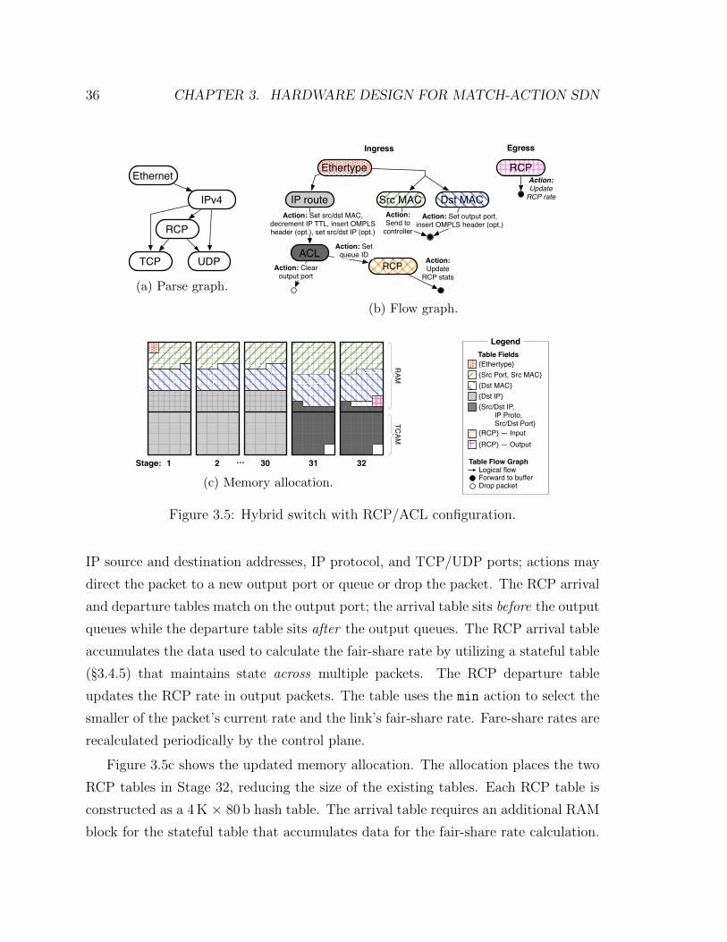
36 CHAPTER 3. HARDWARE DESIGN FOR MATCH-ACTION SDN
IPv4
RCP
TCP UDP
Ethernet
(a) Parse graph.
IP route
Ethertype
Src MAC Dst MAC
RCPACL
Action: Set src/dst MAC, decrement IP TTL, insert OMPLS header (opt.), set src/dst IP (opt.)
Action: Set queue ID
Action: Clear output port
Action: Update
RCP stats
Action: Send to
controller
RCPAction: Update
RCP rate
EgressIngress
Action: Set output port,insert OMPLS header (opt.)
(b) Flow graph.
31 321 2 30…Stage:
TCAM
RAM
(c) Memory allocation.
Legend
Logical flow
Drop packetForward to buffer
Table Flow Graph
{Ethertype}
{RCP} — Input
{Dst IP}
{Src Port, Src MAC}{Dst MAC}
{Src/Dst IP, IP Proto, Src/Dst Port}
Table Fields
{RCP} — Output
Figure 3.5: Hybrid switch with RCP/ACL configuration.
IP source and destination addresses, IP protocol, and TCP/UDP ports; actions may
direct the packet to a new output port or queue or drop the packet. The RCP arrival
and departure tables match on the output port; the arrival table sits before the output
queues while the departure table sits after the output queues. The RCP arrival table
accumulates the data used to calculate the fair-share rate by utilizing a stateful table
(§3.4.5) that maintains state across multiple packets. The RCP departure table
updates the RCP rate in output packets. The table uses the min action to select the
smaller of the packet’s current rate and the link’s fair-share rate. Fare-share rates are
recalculated periodically by the control plane.
Figure 3.5c shows the updated memory allocation. The allocation places the two
RCP tables in Stage 32, reducing the size of the existing tables. Each RCP table is
constructed as a 4 K × 80 b hash table. The arrival table requires an additional RAM
block for the stateful table that accumulates data for the fair-share rate calculation.
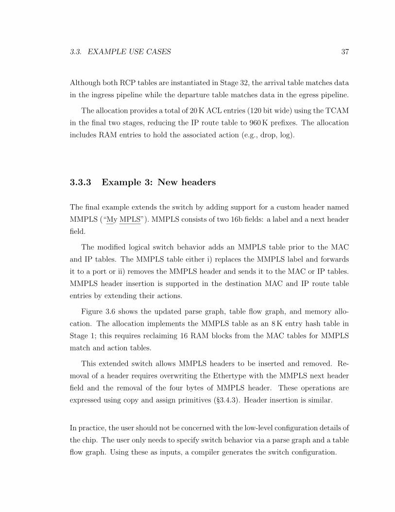
3.3. EXAMPLE USE CASES 37
Although both RCP tables are instantiated in Stage 32, the arrival table matches data
in the ingress pipeline while the departure table matches data in the egress pipeline.
The allocation provides a total of 20 K ACL entries (120 bit wide) using the TCAM
in the final two stages, reducing the IP route table to 960 K prefixes. The allocation
includes RAM entries to hold the associated action (e.g., drop, log).
3.3.3 Example 3: New headers
The final example extends the switch by adding support for a custom header named
MMPLS (“My MPLS”). MMPLS consists of two 16b fields: a label and a next header
field.
The modified logical switch behavior adds an MMPLS table prior to the MAC
and IP tables. The MMPLS table either i) replaces the MMPLS label and forwards
it to a port or ii) removes the MMPLS header and sends it to the MAC or IP tables.
MMPLS header insertion is supported in the destination MAC and IP route table
entries by extending their actions.
Figure 3.6 shows the updated parse graph, table flow graph, and memory allo-
cation. The allocation implements the MMPLS table as an 8 K entry hash table in
Stage 1; this requires reclaiming 16 RAM blocks from the MAC tables for MMPLS
match and action tables.
This extended switch allows MMPLS headers to be inserted and removed. Re-
moval of a header requires overwriting the Ethertype with the MMPLS next header
field and the removal of the four bytes of MMPLS header. These operations are
expressed using copy and assign primitives (§3.4.3). Header insertion is similar.
In practice, the user should not be concerned with the low-level configuration details of
the chip. The user only needs to specify switch behavior via a parse graph and a table
flow graph. Using these as inputs, a compiler generates the switch configuration.
38 CHAPTER 3. HARDWARE DESIGN FOR MATCH-ACTION SDN
IPv4
RCP
TCP UDP
Ethernet
MMPLS
(a) Parse graph.
IP route
Ethertype
Src MAC Dst MAC
RCP
ACL
Action: Set src/dst MAC, decrement IP TTL, insert OMPLS header (opt.), set src/dst IP (opt.)
Action: Set queue IDAction:
Clear output port
Action: Update
RCP stats
Action: Set output port,insert OMPLS header (opt.)
Action: Send to
controller
RCPAction: Update
RCP rate
MMPLSAction: Pop OMPLS
headerAction: Set output portAction: Pop
OMPLS header
EgressIngress
(b) Flow graph.
31 321 2 30…Stage:
TCAM
RAM
(c) Memory allocation.
Legend
Logical flow
Drop packetForward to buffer
Table Flow Graph
{Ethertype}
{RCP} — Input
{Dst IP}
{Src Port, Src MAC}{Dst MAC}
{Src/Dst IP, IP Proto, Src/Dst Port}
Table Fields
{RCP} — OutputMMPLS
Figure 3.6: Hybrid switch with RCP/ACL/MMPLS configuration.
3.4 Chip design
The focus thus far has been the logical abstraction of an RMT forwarding plane that is
convenient for network users. The remainder of this chapter describes implementation
design details for a 640 Gb/s RMT switch (64 ports × 10 Gb/s).
The switch operating frequency was chosen to be 1 GHz. This frequency allows a
single pipeline to process all input data from all input ports, rather than requiring
multiple slower parallel pipelines. The 1 GHz frequency is slightly above the maximum
packet arrival of 960 M packets/s for the switch, which occurs when back-to-back 64-
byte minimum-sized packet streams arrive simultaneously on all 64 ports at 10 Gb/s.
The use of multiple parallel pipelines increases area requirements and/or reduces flow
table sizes because each pipeline requires its own set of memories. Figure 3.7 shows a

3.4. CHIP DESIGN 39
block diagram of the switch chip; this design closely resembles the RMT architectural
diagram of Figure 3.2a.
Egress processingIngress processing
...
...
Ingress Deparser
MatchStage
1
Match Stage
32
Ingress Parsers
Common data buffer
...Egress
Deparser
MatchStage
1
Match Stage
32
Egress Parsers
...
packetpointer
(enqueue)
packetpointer
(dequeue)
packetdata
packetdata
OutputCh. 1
OutputCh. 64
InputCh. 64
InputCh. 1
...
queues
... ...
Figure 3.7: Switch chip block diagram.
Input signals arrive at 64 channels of 10 Gb/s SerDes (serializer-deserializer) I/O
modules. Four 10 Gb/s channels may be ganged together to create a 40 Gb/s channel.
The signals from the SerDes modules pass through modules that perform low-level
signalling and MAC (medium access control) functions such as checksum generation
and verification.
Data flows next to the parsers. Each programmable parser instance processes data
at 40 Gb/s, requiring a total of 16 ingress parsers to process data for all channels.
Each 40 Gb/s parser instance processes either four 10 Gb/s channels or one 40 Gb/s
channel. Many different combinations of headers may be present in received packets.
Each parser identifies the headers present in each packet and extracts fields of interest,
placing extracted fields into the packet header vector; the size of the vector is 4 Kb.
The switch configuration step assigns field locations within the vector, with fields
from multiple instances of a header (e.g., multiple MPLS tags or inner and outer IP
fields) being assigned unique locations. This configuration process ensures that each
field has a unique fixed location within the vector.
The switch multiplexes the input parser results into a single stream and feeds it
to the ingress match pipeline. The ingress match pipeline consists of 32 sequential
match stages. Deparsers at the end of the match pipeline merge data from the packet
header vector back into each packet.
A large shared on-chip buffer and associated queueing system provides storage to
accommodate queuing delays caused by output port oversubscription. Packet data is
stored in the data buffer while pointers to that data are kept in 2 K queues per port.
The data buffer allocates storage to channels as required. Channels at the egress

40 CHAPTER 3. HARDWARE DESIGN FOR MATCH-ACTION SDN
of the data buffer request data from the buffer in turn using configurable queueing
policies.
Data retrieved from the buffer flows through an egress pipeline. An egress parser
extracts fields into the packet header vector, and that vector flows through 32 match
stages before being recombined with the packet at a deparser. Packets are then
directed to the appropriate output ports where they are driven off chip by 64 SerDes
output channels.
While a separate 32-stage egress processing pipeline seems like overkill, the egress
and ingress pipelines actually share the same match tables and thus the costs are
minimal. Egress processing is beneficial as it allows a multicast packet to be cus-
tomized by port (e.g., setting a congestion bit or MAC destination on a per-port
basis) without storing several different packet copies in the buffer.
Each of the major components in the design is described in more detail below.
3.4.1 Configurable parser
The parser accepts the incoming packet data and produces the 4 Kb packet header
vector as its output. The switch configuration process assigns each header field a
unique position within the header vector. The header vector is fed as input data to
the match pipeline. Each parser processes 40 Gb/s, composed of either one 40 Gb/s
stream or four 10 Gb/s streams; a total of 16 ingress and 16 egress parsers are used
to provide the requisite 640 Gb/s parsing throughput.
A user-supplied parse graph (Figure 3.3b) directs parsing. An offline algorithm
converts the parse graph into entries in a 256 entry × 40 b TCAM and associated
RAM. The parser TCAM is completely separate from the match TCAMs used in
each match stage. Each entry matches 32 bits of incoming packet data and 8 bits of
parser state. The ternary matching provided by the TCAM allows an entry to match
on a subset of bits in the incoming packet stream; for example, an entry can match
on just a 16-bit Ethertype value by wildcarding the other 16 bits of input.
The result of a TCAM match triggers an action, which updates the parser state,
shifts the incoming data a specified number of bytes, and directs the outputting of

3.4. CHIP DESIGN 41
one or more fields from positions in the input packet to fixed positions in the packet
header vector. This loop repeats to parse each packet. The design optimizes the
critical loop by pulling critical update data, such as input shift count and next parser
state, out of RAM and into the TCAM output prioritization logic. The parser’s single
cycle loop matches fields at 32 Gb/s, translating to a much higher throughput because
not all fields need matching by the parser. A single parser instance easily supports a
40 Gb/s packet stream.
The design of packet parsers is the subject of Chapter 4. That chapter provides
greater detail on the design and operation of the programmable parser, the choice
of design parameters, and the algorithm that converts parse graphs into flow table
entries.
3.4.2 Configurable match memories
Each match stage contains two 640 bit wide match units: one is a TCAM for ternary
matches, and the other is an SRAM-based hash table for exact matches. The exact
match table unit aggregates eight 80-bit subunits while the ternary table unit aggre-
gates sixteen 40-bit subunits. Each subunit can be run independently for a narrow
table, in parallel with other subunits for wider tables, or ganged together in series
with other subunits into deeper tables. An input crossbar supplies match data to each
subunit by selecting fields from the 4 Kb packet header vector. As §3.2.1 describes,
the switch can combine tables in adjacent match stages to make larger tables. In the
limit, all 32 stages can be combined to create a single table.
The ingress and egress match pipelines of Figure 3.7 are actually the same phys-
ical block. The design shares the pipeline at a fine grain between ingress and egress
processing; a single physical stage can simultaneously host ingress and egress tables
(Figure 3.2b). To do this, the switch configuration process statically assigns each
packet header vector field, action unit, and memory block to ingress or egress pro-
cessing. Ingress fields in the vector are populated by ingress parsers, matched on by
ingress memories, and modified by ingress action units. Egress fields are treated in a
42 CHAPTER 3. HARDWARE DESIGN FOR MATCH-ACTION SDN
similar manner. This static allocation of resources prevents contention issues because
each resource is owned exclusively by either ingress or egress.
Each physical match stage contains 106 RAM blocks, each of which is 1 K entries
× 112 b. Hash match table entries, actions, and statistics all utilize the same RAM
blocks. The fraction of blocks assigned for each purpose are configurable.
Exact match tables utilize the Cuckoo hash algorithm [37,64,96]. Each table uses
a minimum of four-way hashing, with each way using a separate RAM block; the
smallest hash table therefore consists of 4 × 1 K entries. The hash table performs
reads deterministically in one cycle, with all ways accessed in parallel. Ternary match
tables are implemented using the TCAM blocks; each match stage contains 16 TCAM
blocks of 2 K entries × 40 b.
Each match stage places match values, actions, and statistics in separate RAM
blocks; this allows the same action and statistics mechanisms to be used for hash and
ternary matches. Every hash and ternary entry contains a pointer to action memory,
an action size, a pointer to instruction memory, and a next-table address. The design
requires actions to be decomposed into operators and operands; operators are placed
in instruction memory while operands are placed in action memory. For example,
the action “Set VLAN to 51” is decomposed into the operator “Set VLAN” and the
operand “51.” The design places instructions (composed of operators) in a dedicated
instruction memory within each stage and places operands in action memory allocated
from the 106 RAM blocks.
The design supports packet and byte statistics counters for each flow table entry,
as specified in current OpenFlow specifications. Off-chip DRAM stores full 64-bit
versions of these counters while the 1 K match stage RAM blocks store limited reso-
lution counters on-chip. The switch uses the LR(T) algorithm [99] to update off-chip
counters; LR(T) ensures acceptable DRAM update rates. The design allows counters
for either two or three flow entries to be stored in each statistics word; this choice
provides a trade-off between statistics memory cost and DRAM update rate. Each
statistics counter increment is a read-modify-write operation, requiring one memory
3.4. CHIP DESIGN 43
read and one memory write. The memory is single-ported, so a second memory port
is synthesized by adding one memory bank1.
3.4.3 Configurable action engine
The action engine provides separate processing units for each packet header field to
enable concurrent update of all fields (Figure 3.2c). The packet header vector contains
64, 96, and 64 words of 8 bits, 16 bits, and 32 bits, respectively, with an associated
valid bit for each field. The action engine can combine processing units for smaller
words to execute a larger field operation—e.g., two 8-bit units can merge to operate
on their data as a single 16-bit field.
The action engine within a stage executes one VLIW instruction per packet,
with each VLIW instruction containing one operation for each processing unit. As a
consequence, the action engine applies only one operation per field to each packet. A
“null” operation is applied to fields that do not require modification.
The processing units must provide sufficiently rich actions to support current and
future packet processing needs while being sufficiently limited to enable operation at
the desired throughput and to avoid excessive resource consumption. An analysis
of existing protocol behaviors and the operations supported by OpenFlow helped to
identify an appropriate set of primitive operations. Current protocol operations vary
in complexity; the simpler actions include setting and decrementing fields while com-
plex operations include PBB encapsulation and inner-to-outer field copies. Complex
operations can be subroutines at low speeds but must be flattened into single-cycle
operations at the 1 GHz clock rate using a carefully chosen instruction set.
Table 3.1 lists a subset of the action instruction set. The logical, arithmetic,
and shift instructions are self-explanatory. Deposit-byte enables depositing an ar-
bitrary field from anywhere in a source word to anywhere in a background word.
Rot-mask-merge independently byte rotates two sources, then merges them accord-
ing to a byte mask; it is useful in performing IPv6 to IPv4 address translation [4].
Bitmasked-set is useful for selective metadata updates; it requires three sources: the
1S. Iyer. Memoir Systems. Private communication, Dec. 2010.
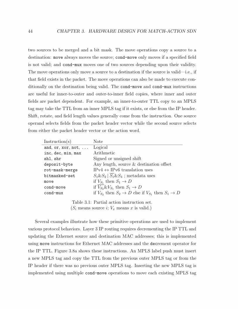
44 CHAPTER 3. HARDWARE DESIGN FOR MATCH-ACTION SDN
two sources to be merged and a bit mask. The move operations copy a source to a
destination: move always moves the source; cond-move only moves if a specified field
is not valid; and cond-mux moves one of two sources depending upon their validity.
The move operations only move a source to a destination if the source is valid—i.e., if
that field exists in the packet. The move operations can also be made to execute con-
ditionally on the destination being valid. The cond-move and cond-mux instructions
are useful for inner-to-outer and outer-to-inner field copies, where inner and outer
fields are packet dependent. For example, an inner-to-outer TTL copy to an MPLS
tag may take the TTL from an inner MPLS tag if it exists, or else from the IP header.
Shift, rotate, and field length values generally come from the instruction. One source
operand selects fields from the packet header vector while the second source selects
from either the packet header vector or the action word.
Instruction(s) Noteand, or, xor, not, ... Logicalinc, dec, min, max Arithmeticshl, shr Signed or unsigned shiftdeposit-byte Any length, source & destination offsetrot-mask-merge IPv4 ↔ IPv6 translation usesbitmasked-set S1&S2 | S1&S3 ; metadata usesmove if VS1 then S1 → Dcond-move if VS2&VS1 then S1 → Dcond-mux if VS2 then S2 → D else if VS1 then S1 → D
Table 3.1: Partial action instruction set.(Si means source i; Vx means x is valid.)
Several examples illustrate how these primitive operations are used to implement
various protocol behaviors. Layer 3 IP routing requires decrementing the IP TTL and
updating the Ethernet source and destination MAC addresses; this is implemented
using move instructions for Ethernet MAC addresses and the decrement operator for
the IP TTL. Figure 3.8a shows these instructions. An MPLS label push must insert
a new MPLS tag and copy the TTL from the previous outer MPLS tag or from the
IP header if there was no previous outer MPLS tag. Inserting the new MPLS tag is
implemented using multiple cond-move operations to move each existing MPLS tag
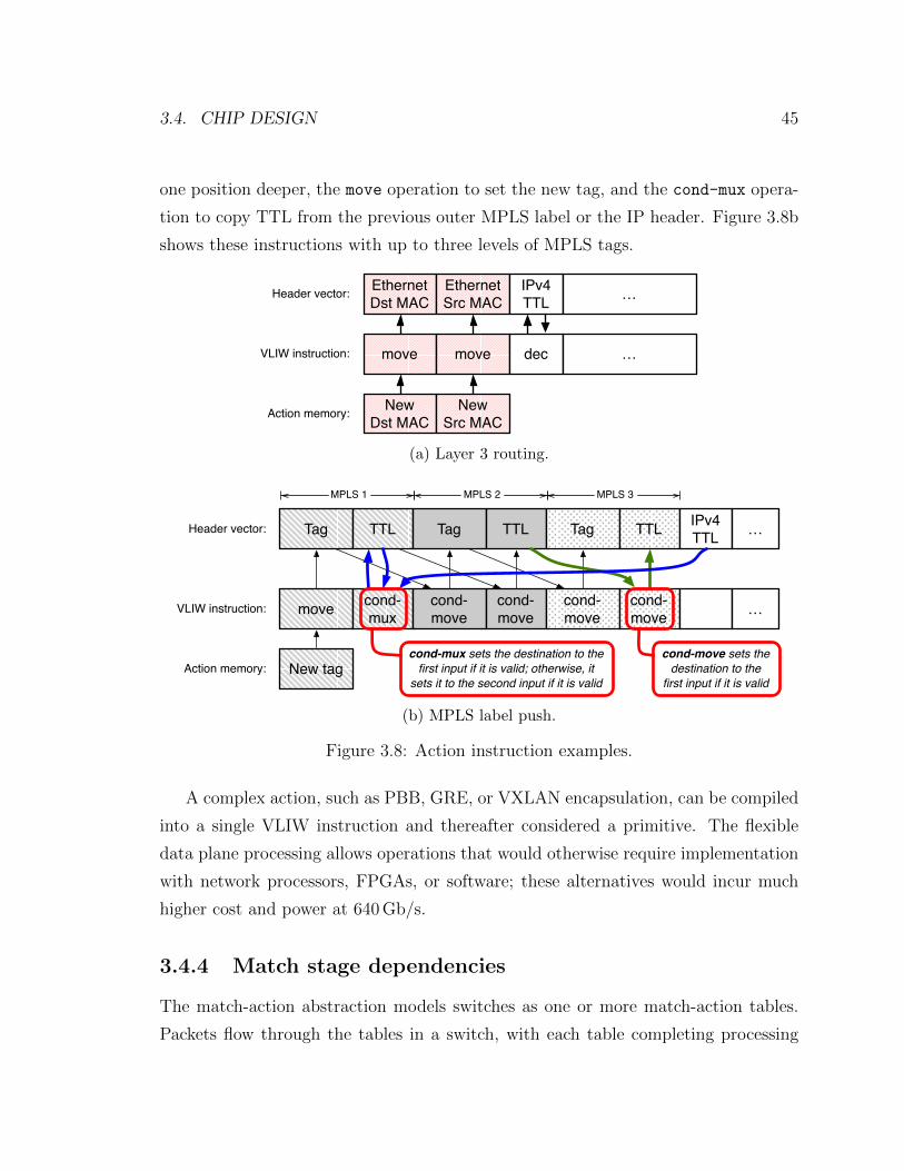
3.4. CHIP DESIGN 45
one position deeper, the move operation to set the new tag, and the cond-mux opera-
tion to copy TTL from the previous outer MPLS label or the IP header. Figure 3.8b
shows these instructions with up to three levels of MPLS tags.
Header vector:
VLIW instruction:
Ethernet Dst MAC
Ethernet Src MAC
IPv4 TTL
move move dec …
…
Action memory: NewDst MAC
NewSrc MAC
(a) Layer 3 routing.
Header vector:
VLIW instruction:
Tag TTL
Action memory:
Tag TTL Tag TTL IPv4 TTL
MPLS 1 MPLS 2 MPLS 3
move cond-mux
cond-move
cond-move
cond-move
cond-move
New tag
…
…
cond-mux sets the destination to the first input if it is valid; otherwise, it
sets it to the second input if it is valid
cond-move sets the destination to the
first input if it is valid
(b) MPLS label push.
Figure 3.8: Action instruction examples.
A complex action, such as PBB, GRE, or VXLAN encapsulation, can be compiled
into a single VLIW instruction and thereafter considered a primitive. The flexible
data plane processing allows operations that would otherwise require implementation
with network processors, FPGAs, or software; these alternatives would incur much
higher cost and power at 640 Gb/s.
3.4.4 Match stage dependencies
The match-action abstraction models switches as one or more match-action tables.
Packets flow through the tables in a switch, with each table completing processing

46 CHAPTER 3. HARDWARE DESIGN FOR MATCH-ACTION SDN
of each packet before sending the packet to the next table. Mechanisms may option-
ally be included to allow skipping tables. The switch configuration can easily ensure
correctness by mapping logical tables to separate physical stages, and by requiring
physical match stage i to complete processing of packet header vector P before pro-
cessing commences in stage i+ 1. This unfortunately wastes memory resources inside
physical stages and introduces excessive latency.
The switch can reduce latency and resource wastage by allowing multiple tables
to process packets concurrently. Not all processing can overlap; the key is to identify
dependencies between match tables to determine what may overlap. Three types of
dependencies exist: match dependencies, action dependencies, and successor depen-
dencies ; each of these is described in depth below.
Each dependency type permits a different degree of overlap. This comes about
because processing within a single stage occurs in three phases over multiple clock
cycles. Matching occurs first, then actions are applied, and finally, the modified packet
header vector is output. The first two phases, match and action application, require
several clock cycles each. The different dependency types allow differing degrees of
overlap between phases in sequential tables.
Match dependencies
Match dependencies occur when a match stage modifies a packet header field and a
subsequent stage matches upon that field. In this case, the first stage must complete
match and action processing before the subsequent stage can commence processing.
No time overlap is possible in processing the two match stages (Figure 3.9a). Failure
to prevent overlap results in “old” data being matched: matching in stage i + 1
commences before stage i updates the packet header vector.
Figure 3.9a shows a small time gap between the end of first stage execution and
the beginning of the second stage execution. This gap is the transport delay, the time
it takes to physically move signals from the output of the first stage to the input of
the second stage on chip.
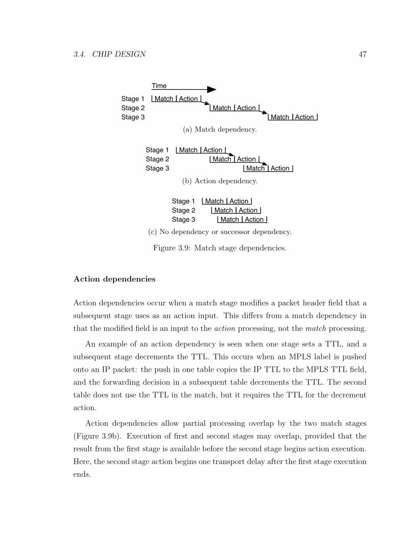
3.4. CHIP DESIGN 47
Stage 1Stage 2Stage 3
Match ActionMatch Action
Match Action
Time
(a) Match dependency.
Match ActionMatch Action
Match Action
Stage 1Stage 2Stage 3
(b) Action dependency.
Match ActionMatch Action
Match Action
Stage 1Stage 2Stage 3
(c) No dependency or successor dependency.
Figure 3.9: Match stage dependencies.
Action dependencies
Action dependencies occur when a match stage modifies a packet header field that a
subsequent stage uses as an action input. This differs from a match dependency in
that the modified field is an input to the action processing, not the match processing.
An example of an action dependency is seen when one stage sets a TTL, and a
subsequent stage decrements the TTL. This occurs when an MPLS label is pushed
onto an IP packet: the push in one table copies the IP TTL to the MPLS TTL field,
and the forwarding decision in a subsequent table decrements the TTL. The second
table does not use the TTL in the match, but it requires the TTL for the decrement
action.
Action dependencies allow partial processing overlap by the two match stages
(Figure 3.9b). Execution of first and second stages may overlap, provided that the
result from the first stage is available before the second stage begins action execution.
Here, the second stage action begins one transport delay after the first stage execution
ends.

48 CHAPTER 3. HARDWARE DESIGN FOR MATCH-ACTION SDN
Successor dependencies
As detailed earlier, each flow entry contains a next-table field that specifies the next
table to execute; absence of a next table indicates the end of table processing. Succes-
sor dependencies occur when execution of a match stage is predicated on the result of
an earlier stage. Successor dependencies and predication are illustrated via a simple
example. Assume a simple setup with three successive tables A, B, and C. Processing
begins with table A; each table entry in A may specify B, C, or nothing as the next
table. Successor dependencies exist between A and B, and between A and C. Table
B is executed only when the next table is B, so B’s execution is predicated by the
successor indication from A.
Although B’s execution is predicated on A, the chip can speculatively execute B.
Results from B are only committed once all predication qualifications are resolved.
A match stage can resolve predication inline between its 16 tables, and two adjacent
stages can resolve predication using the inter-stage transport delay. In the latter case,
the pipeline offsets execution of successive stages only by the transport delay (Fig-
ure 3.9c). Successor dependencies incur no additional delay in this design. Contrast
this with a naıve implementation that delays execution of subsequent tables until
successors are positively identified, thereby introducing as much delay as a match
dependency.
The simple example of three tables A, B, and C mirrors the hybrid L2/L3 switch
example in §3.3.1. Execution begins with the Ethertype table: the Ethertype is
matched to identify whether the packet contains an IP header. If the packet does
contain an IP header, then execution proceeds with the L3 route table; otherwise,
execution proceeds with the L2 destination MAC table.
No dependencies
Execution of multiple match stages can be concurrent when no dependencies exist
between them. Figure 3.9c applies in this case, where the executions of consecutive
stages are offset only by the transport delay.
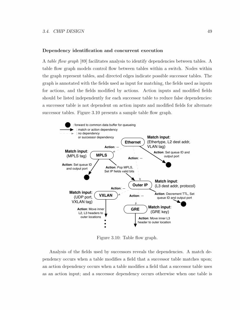
3.4. CHIP DESIGN 49
Dependency identification and concurrent execution
A table flow graph [89] facilitates analysis to identify dependencies between tables. A
table flow graph models control flow between tables within a switch. Nodes within
the graph represent tables, and directed edges indicate possible successor tables. The
graph is annotated with the fields used as input for matching, the fields used as inputs
for actions, and the fields modified by actions. Action inputs and modified fields
should be listed independently for each successor table to reduce false dependencies:
a successor table is not dependent on action inputs and modified fields for alternate
successor tables. Figure 3.10 presents a sample table flow graph.
Ethernet
Outer IP
MPLS
GRE
VXLAN
...
Action: Set queue ID and output port Action: Pop MPLS,
Set IP fields valid bits
Action: —
Action: —
Action: —
Action: —
Action: Set queue ID and output port
Action: Decrement TTL, Set queue ID and output port
Action: Move inner L3 header to outer location
Action: Move inner L2, L3 headers to
outer locations
Match input:{Ethertype, L2 dest addr,VLAN tag}
Match input:{MPLS tag}
Match input:{L3 dest addr, protocol}
Match input:{UDP port,
VXLAN tag}Match input:
{GRE key}
: forward to common data buffer for queueing: match or action dependency: no dependency or successor dependency
Figure 3.10: Table flow graph.
Analysis of the fields used by successors reveals the dependencies. A match de-
pendency occurs when a table modifies a field that a successor table matches upon;
an action dependency occurs when a table modifies a field that a successor table uses
as an action input; and a successor dependency occurs otherwise when one table is
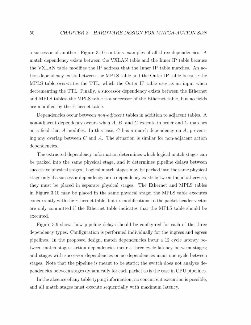
50 CHAPTER 3. HARDWARE DESIGN FOR MATCH-ACTION SDN
a successor of another. Figure 3.10 contains examples of all three dependencies. A
match dependency exists between the VXLAN table and the Inner IP table because
the VXLAN table modifies the IP address that the Inner IP table matches. An ac-
tion dependency exists between the MPLS table and the Outer IP table because the
MPLS table overwrites the TTL, which the Outer IP table uses as an input when
decrementing the TTL. Finally, a successor dependency exists between the Ethernet
and MPLS tables; the MPLS table is a successor of the Ethernet table, but no fields
are modified by the Ethernet table.
Dependencies occur between non-adjacent tables in addition to adjacent tables. A
non-adjacent dependency occurs when A, B, and C execute in order and C matches
on a field that A modifies. In this case, C has a match dependency on A, prevent-
ing any overlap between C and A. The situation is similar for non-adjacent action
dependencies.
The extracted dependency information determines which logical match stages can
be packed into the same physical stage, and it determines pipeline delays between
successive physical stages. Logical match stages may be packed into the same physical
stage only if a successor dependency or no dependency exists between them; otherwise,
they must be placed in separate physical stages. The Ethernet and MPLS tables
in Figure 3.10 may be placed in the same physical stage; the MPLS table executes
concurrently with the Ethernet table, but its modifications to the packet header vector
are only committed if the Ethernet table indicates that the MPLS table should be
executed.
Figure 3.9 shows how pipeline delays should be configured for each of the three
dependency types. Configuration is performed individually for the ingress and egress
pipelines. In the proposed design, match dependencies incur a 12 cycle latency be-
tween match stages; action dependencies incur a three cycle latency between stages;
and stages with successor dependencies or no dependencies incur one cycle between
stages. Note that the pipeline is meant to be static; the switch does not analyze de-
pendencies between stages dynamically for each packet as is the case in CPU pipelines.
In the absence of any table typing information, no concurrent execution is possible,
and all match stages must execute sequentially with maximum latency.
3.4. CHIP DESIGN 51
3.4.5 Other architectural features
Multicast and ECMP
Multicast processing is split between ingress and egress. Ingress processing writes an
output port bit vector field to specify outputs; it may optionally include a tag for
later matching and the number of copies routed to each port. The switch stores a
single copy of each multicast packet in the data buffer, with multiple pointers placed
in the queues. The switch generates copies of the packet when it is injected into the
egress pipeline; here tables may match on the tag, the output port, and a packet copy
count to allow per-port modifications.
ECMP and uECMP processing are similar. Ingress processing writes a bit vector
to indicate possible outputs and, optionally, a weight for each output. The switch
selects the destination when the packet is buffered, allowing it to be enqueued for a
single port. The egress pipeline performs per-port modifications.
Meters and stateful tables
Meters measure and classify flow rates of matching table entries, which can trigger
modification or dropping of packets that exceed set limits. The switch implements
meter tables using match stage unit memories provided for match, action, and statis-
tics. Like statistics memories, meter table memories require two accesses per meter
update in a read-modify-write operation. Each word in a meter table includes allowed
data rates, burst sizes, and bucket levels.
Meters are one example of stateful tables ; these provide a means for an action to
modify state, which is visible to subsequent packets and can be used to modify them.
The design implements a form of stateful counters that can be arbitrarily incremented
and reset. For example, such stateful tables can be used to implement GRE sequence
numbers and OAM [53, 60]. GRE sequence numbers are incremented each time a
packet is encapsulated. In OAM, a switch broadcasts packets at prescribed intervals,
raising an alarm if return packets do not arrive by a specified interval and the counter
52 CHAPTER 3. HARDWARE DESIGN FOR MATCH-ACTION SDN
exceeds a threshold; a packet broadcast increments a counter, and reception of a
return packet resets the counter.
Consistent and atomic updates
The switch associates a version identifier with each packet flowing through the match
pipeline. Each table entry specifies one or more version identifiers that the should
be matched. Version identifiers allow the switch to support consistent updates [100],
where each packet sees either old state or new state across all tables, but not a mixture.
This mechanism also supports atomic updates of multiple rules and associating each
packet with a specific table version and configuration, both of which are useful for
debugging [44].
3.5 Evaluation
The cost of configurability is characterized in terms of the increased area and power of
this design relative to a conventional, less programmable switch chip. Contributions
to the cost by the parser, the match stages, and the action processing are considered
in turn. The comparison culminates in a comparison of total chip area and power in
§3.5.4.
3.5.1 Programmable parser costs
A conventional fixed parser is optimized for one parse graph whereas a programmable
parser must support any user-supplied parse graph. The cost of programmability
is evaluated by comparing gate counts from synthesis for conventional and pro-
grammable designs. Figure 3.11 shows total gate count for a conventional parser
implementing several parse graphs and for the programmable parser. The “big-union”
parse graph is a union of use cases (§4.2) and the “complex” parse graph matches
the resource constraints of the programmable parser. The implementation aggregates
16 instances of a 40 Gb/s parser to provide the desired 640 Gb/s throughput. The
programmable parser contains a 256 × 40 b TCAM and a 256 × 128 b action RAM.
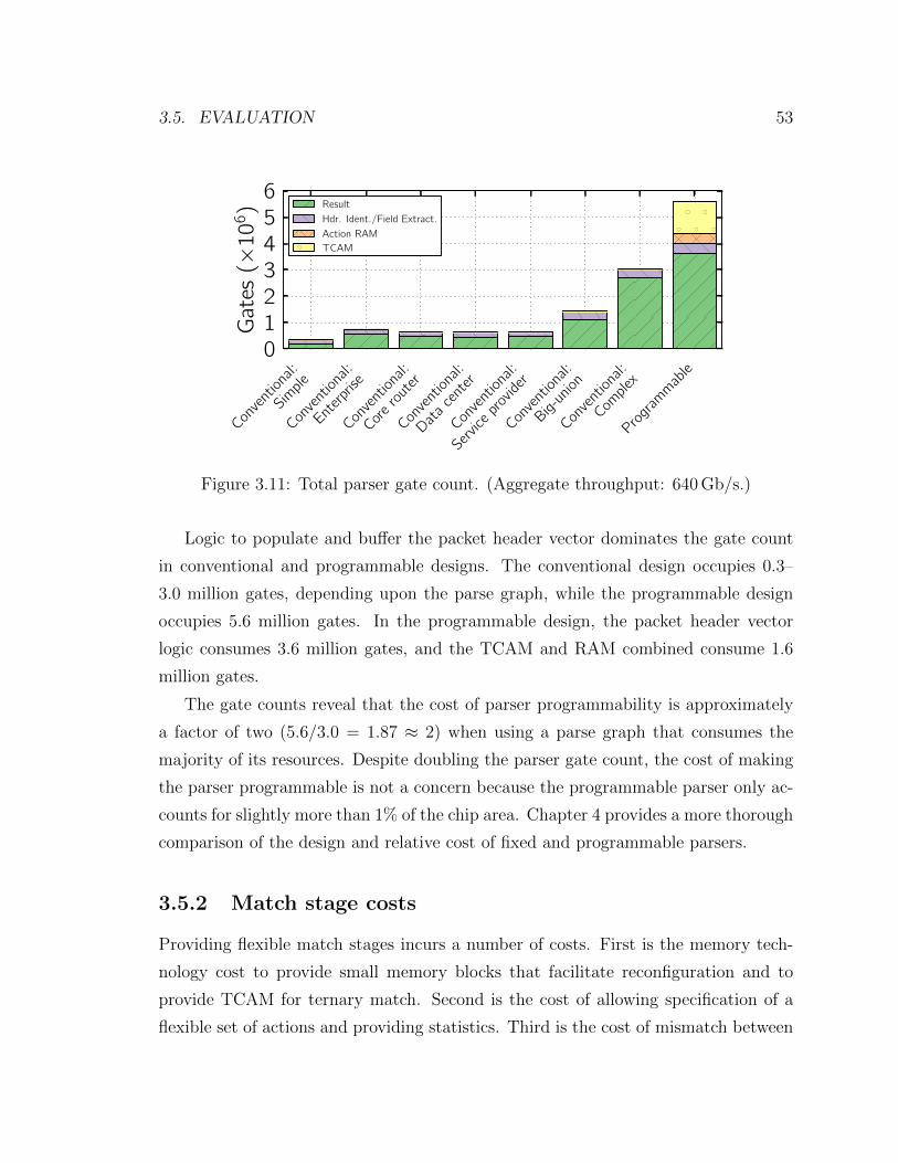
3.5. EVALUATION 53
Conventio
nal:
Simple
Conventio
nal:
Enterp
rise
Conventio
nal:
Corero
uter
Conventio
nal:
Data
cente
r
Conventio
nal:
Servic
epro
vider
Conventio
nal:
Big-u
nion
Conventio
nal:
Comple
x
Progra
mm
able0123456
Gat
es(×
10
6) Result
Hdr. Ident./Field Extract.
Action RAM
TCAM
Figure 3.11: Total parser gate count. (Aggregate throughput: 640 Gb/s.)
Logic to populate and buffer the packet header vector dominates the gate count
in conventional and programmable designs. The conventional design occupies 0.3–
3.0 million gates, depending upon the parse graph, while the programmable design
occupies 5.6 million gates. In the programmable design, the packet header vector
logic consumes 3.6 million gates, and the TCAM and RAM combined consume 1.6
million gates.
The gate counts reveal that the cost of parser programmability is approximately
a factor of two (5.6/3.0 = 1.87 ≈ 2) when using a parse graph that consumes the
majority of its resources. Despite doubling the parser gate count, the cost of making
the parser programmable is not a concern because the programmable parser only ac-
counts for slightly more than 1% of the chip area. Chapter 4 provides a more thorough
comparison of the design and relative cost of fixed and programmable parsers.
3.5.2 Match stage costs
Providing flexible match stages incurs a number of costs. First is the memory tech-
nology cost to provide small memory blocks that facilitate reconfiguration and to
provide TCAM for ternary match. Second is the cost of allowing specification of a
flexible set of actions and providing statistics. Third is the cost of mismatch between
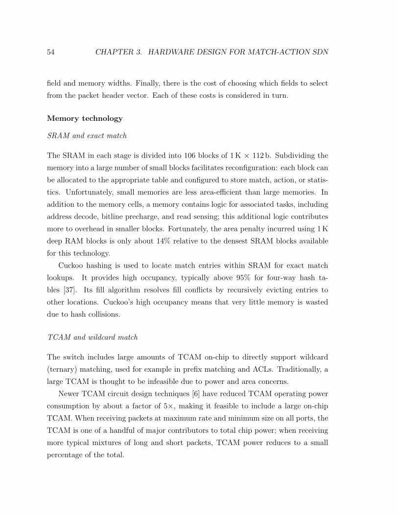
54 CHAPTER 3. HARDWARE DESIGN FOR MATCH-ACTION SDN
field and memory widths. Finally, there is the cost of choosing which fields to select
from the packet header vector. Each of these costs is considered in turn.
Memory technology
SRAM and exact match
The SRAM in each stage is divided into 106 blocks of 1 K × 112 b. Subdividing the
memory into a large number of small blocks facilitates reconfiguration: each block can
be allocated to the appropriate table and configured to store match, action, or statis-
tics. Unfortunately, small memories are less area-efficient than large memories. In
addition to the memory cells, a memory contains logic for associated tasks, including
address decode, bitline precharge, and read sensing; this additional logic contributes
more to overhead in smaller blocks. Fortunately, the area penalty incurred using 1 K
deep RAM blocks is only about 14% relative to the densest SRAM blocks available
for this technology.
Cuckoo hashing is used to locate match entries within SRAM for exact match
lookups. It provides high occupancy, typically above 95% for four-way hash ta-
bles [37]. Its fill algorithm resolves fill conflicts by recursively evicting entries to
other locations. Cuckoo’s high occupancy means that very little memory is wasted
due to hash collisions.
TCAM and wildcard match
The switch includes large amounts of TCAM on-chip to directly support wildcard
(ternary) matching, used for example in prefix matching and ACLs. Traditionally, a
large TCAM is thought to be infeasible due to power and area concerns.
Newer TCAM circuit design techniques [6] have reduced TCAM operating power
consumption by about a factor of 5×, making it feasible to include a large on-chip
TCAM. When receiving packets at maximum rate and minimum size on all ports, the
TCAM is one of a handful of major contributors to total chip power; when receiving
more typical mixtures of long and short packets, TCAM power reduces to a small
percentage of the total.
3.5. EVALUATION 55
A TCAM’s area is typically six to seven times that of an equivalent bitcount
SRAM. However, a flow entry consists of more than just the match. Binary and
ternary flow entries both have other bits associated with them, including action
memory; statistics counters; and instruction, action, and next-table pointers. For
example, an IP routing entry may contain a 32-bit IP prefix in TCAM, a 48-bit
statistics counter in SRAM, and a 16-bit action memory for specifying the next hop
in SRAM; the TCAM accounts for a third of the total memory bitcount, bringing the
TCAM area penalty down to around three times that of SRAM.
Although a factor of three is significant, IPv4 longest prefix match (LPM), IPv6
LPM, and ACLs are major use cases in existing switches. Given the importance of
these matches, it seems prudent to include significant TCAM resources. LPM lookups
can be performed in SRAM using special purpose algorithms [22], but it is difficult
or impossible for these approaches to achieve the single-cycle latency of TCAMs for
a 32-bit or 128-bit LPM.
The ratio of ternary to binary table capacity is an important implementation
decision with significant cost implications, for which there is currently little real world
feedback. The ternary to binary ratio selected for this design is 1:2. The included
TCAM resources allow roughly 1 M IPv4 prefixes or 300 K 120-bit ACL entries.
Action specification and statistics
From a user’s perspective, the primary purpose of the SRAM blocks is the storage of
match values. Ideally, memory of size m can provide a match table of width w and
depth d, where w × d = m. Use of the SRAM for any purpose other than storing
match values is overhead to the user.
Unfortunately, the SRAM blocks must also store actions and statistics for each
flow entry. The amount of memory required for actions and statistics is use case
dependent. For example, not all applications require statistics, so statistics can be
disabled when not needed.
Overhead exists even within the blocks allocated to store match values. Each entry
in the match memory contains the match value and several additional data items: a
pointer to action memory (13 b), an action size (5 b), a pointer to instruction memory
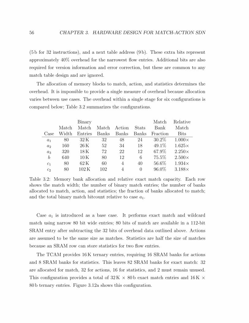
56 CHAPTER 3. HARDWARE DESIGN FOR MATCH-ACTION SDN
(5 b for 32 instructions), and a next table address (9 b). These extra bits represent
approximately 40% overhead for the narrowest flow entries. Additional bits are also
required for version information and error correction, but these are common to any
match table design and are ignored.
The allocation of memory blocks to match, action, and statistics determines the
overhead. It is impossible to provide a single measure of overhead because allocation
varies between use cases. The overhead within a single stage for six configurations is
compared below; Table 3.2 summarizes the configurations.
Binary Match RelativeMatch Match Match Action Stats Bank Match
Case Width Entries Banks Banks Banks Fraction Bitsa1 80 32 K 32 48 24 30.2% 1.000×a2 160 26 K 52 34 18 49.1% 1.625×a3 320 18 K 72 22 12 67.9% 2.250×b 640 10 K 80 12 6 75.5% 2.500×c1 80 62 K 60 4 40 56.6% 1.934×c2 80 102 K 102 4 0 96.0% 3.188×
Table 3.2: Memory bank allocation and relative exact match capacity. Each rowshows the match width; the number of binary match entries; the number of banksallocated to match, action, and statistics; the fraction of banks allocated to match;and the total binary match bitcount relative to case a1.
Case a1 is introduced as a base case. It performs exact match and wildcard
match using narrow 80 bit wide entries; 80 bits of match are available in a 112-bit
SRAM entry after subtracting the 32 bits of overhead data outlined above. Actions
are assumed to be the same size as matches. Statistics are half the size of matches
because an SRAM row can store statistics for two flow entries.
The TCAM provides 16 K ternary entries, requiring 16 SRAM banks for actions
and 8 SRAM banks for statistics. This leaves 82 SRAM banks for exact match: 32
are allocated for match, 32 for actions, 16 for statistics, and 2 must remain unused.
This configuration provides a total of 32 K × 80 b exact match entries and 16 K ×80 b ternary entries. Figure 3.12a shows this configuration.

3.5. EVALUATION 57
Excluding the 24 banks used for ternary actions and statistics, only 40% of the
banks used for binary operations are match tables, indicating an overhead of 150%.
Compounding this with the 40% overhead in the match tables, the total binary over-
head is 190%. In other words, only a third of the RAM bits are being used for match
values.
(a) (b) (c)
: Binary match: Stats
: Binary action: Stats or binary match
: Ternary action: Unused
Figure 3.12: Match stage memory allocation examples.
Cases a2 and a3 increase the match width to 160 and 320 bits, respectively, while
keeping the action width unchanged. Action and statistics memory requirements are
reduced, yielding increased capacity. The 160-bit case requires one action bank and
half a statistics bank for every two match banks, and the 320-bit case requires one
action bank and half a statistics bank for every four match banks.
Case b increases the match width to 640 bits, which is the maximum width sup-
ported within a stage. The 8× wider flow entries allow 80 banks, or 75% of memory
capacity, to be used for exact match. This is 2.5× higher table capacity than the
base case of a1. A match this wide would span many headers, making it less common
than narrower matches. Figure 3.12b shows this configuration.
In many use cases, the number of unique actions to apply is small. For example,
an Ethernet switch forwards each packet to one of its output ports; the number of
unique actions corresponds to the number of ports in this case. Fewer action memories
can be used in scenarios with a small set of unique actions; 4 K would be more than
58 CHAPTER 3. HARDWARE DESIGN FOR MATCH-ACTION SDN
sufficient for the Ethernet switch. Case c1 represents such a scenario. Match tables
are 80 bits wide, allowing 60 banks to be used for match, 40 for statistics, and 4
for actions. This roughly doubles the number of match bits compared with the base
case. Figure 3.12c shows this configuration. Case c2 is similar to case c1, except that
statistics are not required. Eliminating statistics allows 102 banks to be used for
match, corresponding to 96% of total memory capacity.
As one might expect, reducing or eliminating actions or statistics increases the
fraction of memory dedicated to matches. While the cost of configurability may
seem high for some configurations, providing statistics or complex actions in a non-
programmable chip requires a similar amount of memory. The only fundamental costs
that can be directly attributed to programmability are the instruction pointer (5 b)
and the next table address (9 b), which is an overhead of approximately 15%.
Reducing overhead bits in match entries
The action memory pointer, action size, instruction memory pointer, and next ta-
ble address all contribute to match entry overhead. The design implements several
mechanisms to allow reduction of this overhead.
Many tables have a fixed behavior; i.e., all entries apply the same instruction
with different operands, and all have the same next table. For example, all entries
in an L2 switching table specify a forward-to-port instruction for all entries, with
different ports used for each entry. Static values may be configured for an entire table
for the instruction pointer and the next-table address fields, allowing 14 bits to be
reclaimed for match. Match entries can also provide the action value (operand) as an
immediate constant for small values, such as the destination port in the L2 switching
table, eliminating the need for an action pointer and action memory.
A general mechanism provides the ability to specify LSBs for action, instruction,
and next-table addresses via a configurable-width field in the match entry. This allows
a reduced number of different instructions, actions, or next tables, enabling some of
the address bits to be reclaimed.

3.5. EVALUATION 59
A simple mechanism enables these optimizations: match table field field bound-
aries can be flexibly configured, allowing a range of table configurations with arbitrary
sizes for each field, subject to a total bitwidth constraint. Tables with fixed or almost
fixed functions can be efficiently implemented with almost no penalty compared to
traditional switch implementations.
Fragmentation costs
The fragmentation cost arises from the mismatch between field and memory widths:
it is the penalty of bits that remain unused when placing a narrow match value in a
wide memory. For example, a 48-bit Ethernet Destination Address placed in a 112-bit
wide memory wastes more than half the memory. Contrast this with a fixed-function
Ethernet switch that contains 48-bit wide RAM; no memory is wasted in this case.
Fragmentation costs are due entirely to the choice of memory width. The cost could
be eliminated for the Ethernet address example by choosing 48 bits as the base RAM
width; unfortunately, this is the wrong choice for 32-bit IP addresses. It is impossible
to choose a non-trivial width that eliminates fragmentation in a chip designed for
general purpose use and future protocols.
To reduce fragmentation costs, the match architecture allows sets of flow entries
to be packed together without impairing the match function. A standard TCP five-
tuple is 104 bits wide, or 136 bits when the 32-bit match entry overhead is included.
Without packing, a match table requires two memory units to store a single TCP
five-tuple; with packing, a match table requires four memory units of total width 448
bits to store three TCP five-tuples.
Crossbar
A crossbar within each stage selects the match table inputs from the header vector. A
total of 1280 match bits (640 bits each for the TCAM and the hash table) are selected
from the 4 Kb input vector. Each match bit is driven by a 224-input multiplexor,
made from a binary tree of and-or-invert AOI222 gates, costing 0.65µm2 per mux
2An AOI gate has the logic function AB + CD.
60 CHAPTER 3. HARDWARE DESIGN FOR MATCH-ACTION SDN
input. Total crossbar area is 1280 × 224 × 0.65µm2 × 32 stages ≈ 6mm2. The area
computation for the action unit data input muxes is similar.
The combination of variable packing of match entries into multiple data words to
reduce fragmentation costs and variable packing of overhead data into match entries to
reduce action specification costs ensures efficient memory utilization over a wide range
of configurations. These techniques allow the RMT switch to approach the efficiency
of conventional switches for their specific configurations. The RMT switch has the
advantage of supporting a wide range of other configurations, which a conventional
switch cannot.
3.5.3 Costs of action programmability
The pipeline includes an action processor for each packet header vector field in each
match stage, providing a total of around 7,000 action processors. Each action pro-
cessor varies in width from 8 to 32 bits. Fortunately, each processor is quite small: it
resembles an ALU inside a RISC processor. The combined area of all action processors
consumes 7% of the chip.
3.5.4 Area and power costs
Table 3.3 estimates the chip area, broken down by major component. Area is reported
as a percentage of the total die area; cost is reported as an increase in chip area over
an equivalent conventional chip.
The first item, which includes I/O, data buffer, CPU, and so on, is common among
fixed and programmable designs and occupies a similar area in both. The second item
lists the match memories and associated logic. The switch is designed with a large
match table capacity, and, as expected, the memories contribute substantially to chip
area estimates. The final two items, the VLIW action engine and the parser logic,
contribute less than 9% to the total area.
In terms of cost, the match memory and logic contribute the most. The analysis
in §3.5.2 indicated that the small RAM blocks incur a 14% penalty compared to the

3.5. EVALUATION 61
densest SRAM blocks. Allowing for the 15% overhead in match entries, the memory
cost for this chip is estimated at about 8% relative to an equivalent conventional chip.
The action engine and the parser combined are estimated to add an additional 6.2%,
bringing the total area cost to 14.2%.
DieSection Area CostNon-RMT logic; e.g., I/O, buffer, queue, CPU. 37.0% 0.0%Match memory & logic 54.3% 8.0%VLIW action engine 7.4% 5.5%Parser & deparser 1.3% 0.7%
Total cost: 14.2%
Table 3.3: Estimated chip area profile. Area is reported as a percentage of the totaldie area; cost is reported as an increase in chip area over a similar conventional chip.
Table 3.4 shows estimates of the chip power. Estimates assume worst case temper-
ature and process, 100% traffic with a mix of minimum and maximum sized packets,
and all match and action tables filled to capacity. The I/O logic, and hence power, is
identical to a conventional switch. Memory leakage power is proportional to bitcount;
memory leakage power in this chip is slightly higher due to the slightly larger memory.
The remaining items, which total approximately 30%, are less in a conventional chip
because of the reduced functionality in its match pipeline. The programmable chip
dissipates 12.4% more power than a conventional switch, but it performs much more
substantial packet manipulation.
The programmable chip requires roughly equivalent amounts of memory as a con-
ventional chip to perform equivalent functions. Because memory is the dominant
element within the chip, area and power are only a little more than a conventional
chip. The additional area and power costs are a small price to pay for the additional
functionality provided by the switch.
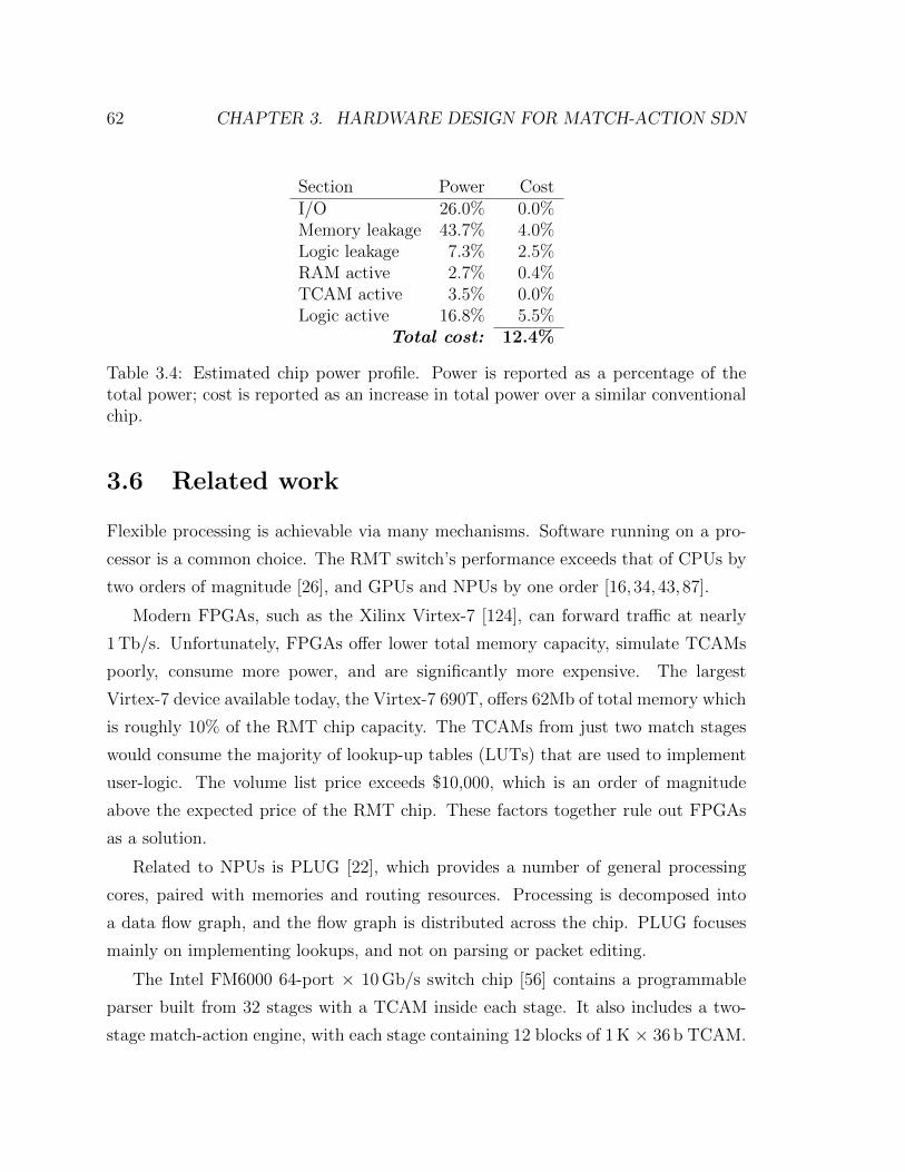
62 CHAPTER 3. HARDWARE DESIGN FOR MATCH-ACTION SDN
Section Power CostI/O 26.0% 0.0%Memory leakage 43.7% 4.0%Logic leakage 7.3% 2.5%RAM active 2.7% 0.4%TCAM active 3.5% 0.0%Logic active 16.8% 5.5%
Total cost: 12.4%
Table 3.4: Estimated chip power profile. Power is reported as a percentage of thetotal power; cost is reported as an increase in total power over a similar conventionalchip.
3.6 Related work
Flexible processing is achievable via many mechanisms. Software running on a pro-
cessor is a common choice. The RMT switch’s performance exceeds that of CPUs by
two orders of magnitude [26], and GPUs and NPUs by one order [16,34,43,87].
Modern FPGAs, such as the Xilinx Virtex-7 [124], can forward traffic at nearly
1 Tb/s. Unfortunately, FPGAs offer lower total memory capacity, simulate TCAMs
poorly, consume more power, and are significantly more expensive. The largest
Virtex-7 device available today, the Virtex-7 690T, offers 62Mb of total memory which
is roughly 10% of the RMT chip capacity. The TCAMs from just two match stages
would consume the majority of lookup-up tables (LUTs) that are used to implement
user-logic. The volume list price exceeds $10,000, which is an order of magnitude
above the expected price of the RMT chip. These factors together rule out FPGAs
as a solution.
Related to NPUs is PLUG [22], which provides a number of general processing
cores, paired with memories and routing resources. Processing is decomposed into
a data flow graph, and the flow graph is distributed across the chip. PLUG focuses
mainly on implementing lookups, and not on parsing or packet editing.
The Intel FM6000 64-port × 10 Gb/s switch chip [56] contains a programmable
parser built from 32 stages with a TCAM inside each stage. It also includes a two-
stage match-action engine, with each stage containing 12 blocks of 1 K × 36 b TCAM.
3.6. RELATED WORK 63
This represents a small fraction of total table capacity, with other tables in a fixed
pipeline.
The latest OpenFlow [94] specification provides an MMT abstraction and imple-
ments elements of the RMT model. However, it does not allow a controller to define
new headers and fields, and its action capability is still limited. It is not certain that
a standard for functionally complete actions is on the way or even possible.

64 CHAPTER 3. HARDWARE DESIGN FOR MATCH-ACTION SDN

Chapter 4
Understanding packet parser
design
Despite their variety, every network device examines the fields in packet headers to
decide what to do with each packet. For example, a router examines the IP destination
address to decide where to send the packet next, a firewall compares several fields
against an access-control list to decide whether to drop a packet, and the RMT switch
in Chapter 3 matches fields against user-defined tables to determine the processing
to perform.
The process of identifying and extracting the appropriate fields in a packet header
is called parsing and is the subject of this chapter. Packet parsing is a non-trivial
process in high speed networks because of the complexity of packet headers, and
design techniques for low-latency streaming parsers are critical for all high speed
networking devices today. Furthermore, applications like the RMT switch require the
ability to redefine the headers understood by the parser.
Packet parsing is challenging because packet lengths and formats vary between
networks and between packets. A basic common structure is one or more headers, a
payload, and an optional trailer. At each step of encapsulation, an identifier included
in the header identifies the type of data subsequent to the header. Figure 4.1 shows
a simple example of a TCP packet.
65
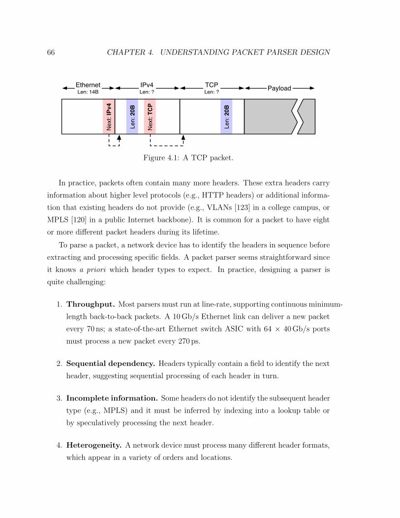
66 CHAPTER 4. UNDERSTANDING PACKET PARSER DESIGN
Nex
t: IPv4
Nex
t: TCP
Len:
20B
Len:
20B
PayloadTCPLen: ?
IPv4Len: ?
EthernetLen: 14B
Figure 4.1: A TCP packet.
In practice, packets often contain many more headers. These extra headers carry
information about higher level protocols (e.g., HTTP headers) or additional informa-
tion that existing headers do not provide (e.g., VLANs [123] in a college campus, or
MPLS [120] in a public Internet backbone). It is common for a packet to have eight
or more different packet headers during its lifetime.
To parse a packet, a network device has to identify the headers in sequence before
extracting and processing specific fields. A packet parser seems straightforward since
it knows a priori which header types to expect. In practice, designing a parser is
quite challenging:
1. Throughput. Most parsers must run at line-rate, supporting continuous minimum-
length back-to-back packets. A 10 Gb/s Ethernet link can deliver a new packet
every 70 ns; a state-of-the-art Ethernet switch ASIC with 64 × 40 Gb/s ports
must process a new packet every 270 ps.
2. Sequential dependency. Headers typically contain a field to identify the next
header, suggesting sequential processing of each header in turn.
3. Incomplete information. Some headers do not identify the subsequent header
type (e.g., MPLS) and it must be inferred by indexing into a lookup table or
by speculatively processing the next header.
4. Heterogeneity. A network device must process many different header formats,
which appear in a variety of orders and locations.

67
5. Programmability. Header formats may change after the parser has been
designed due to a new standard, or because a network operator wants a cus-
tom header field to identify traffic in the network. For example, PBB [54],
VXLAN [73], NVGRE [107], STT [20], and OTV [41] protocols have all been
proposed or ratified in the past five years.
While every network device contains a parser, very few papers have described
their design. Only three papers directly related to parser design have been published
to date: [3, 66, 67]. None of the papers evaluated the trade-offs between area, speed,
and power, and two introduced latency unsuitable for high speed applications; the
third did not evaluate latency. Regular expression matching work is not applicable:
parsing processes a subset of each packet under the control of a parse graph, while
regex matching scans the entire packet for matching expressions.
This chapter has two purposes. First, it informs designers how parser design
decisions impact area, speed, and power via a design space exploration, considering
both hard-coded and reconfigurable designs. It does not propose a single “ideal”
design, because different trade-offs are applicable for different use cases. Second, it
describes a parser design appropriate for use in the RMT switch of Chapter 3.
An engineer setting out to design a parser faces many design choices. A parser can
be built as a single fast unit or as multiple slower units operating in parallel. It can
use a narrow word width, which requires a faster clock, or a wide word width, which
might require processing several headers in one step. It can process a fixed set of
headers, which simplifies the design, or it can provide programmability, which allows
the definition of headers after manufacture. Each design choice potentially impacts
the area and power consumption of the parser.
This chapter answers these questions as follows. First, I describe the parsing pro-
cess in more detail (§4.1) and introduce parse graphs to represent header sequences
and describe the parsing state machine (§4.2). Next, I discuss the design of fixed
and programmable parsers (§4.3), and detail the generation of table entries for pro-
grammable designs (§4.4). Next I present parser design principles, identified through
an analysis of different parser designs (§4.5). I generated the designs using a tool I
built that, given a parse graph, generates parser designs parameterized by processing
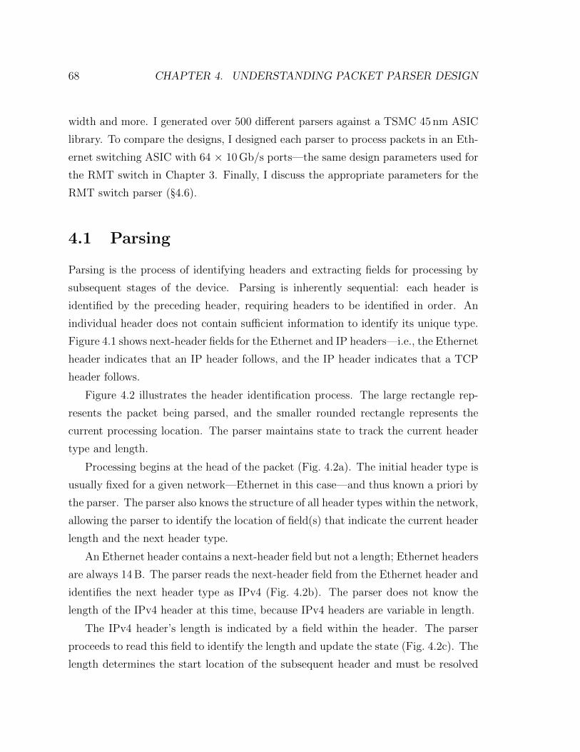
68 CHAPTER 4. UNDERSTANDING PACKET PARSER DESIGN
width and more. I generated over 500 different parsers against a TSMC 45 nm ASIC
library. To compare the designs, I designed each parser to process packets in an Eth-
ernet switching ASIC with 64 × 10 Gb/s ports—the same design parameters used for
the RMT switch in Chapter 3. Finally, I discuss the appropriate parameters for the
RMT switch parser (§4.6).
4.1 Parsing
Parsing is the process of identifying headers and extracting fields for processing by
subsequent stages of the device. Parsing is inherently sequential: each header is
identified by the preceding header, requiring headers to be identified in order. An
individual header does not contain sufficient information to identify its unique type.
Figure 4.1 shows next-header fields for the Ethernet and IP headers—i.e., the Ethernet
header indicates that an IP header follows, and the IP header indicates that a TCP
header follows.
Figure 4.2 illustrates the header identification process. The large rectangle rep-
resents the packet being parsed, and the smaller rounded rectangle represents the
current processing location. The parser maintains state to track the current header
type and length.
Processing begins at the head of the packet (Fig. 4.2a). The initial header type is
usually fixed for a given network—Ethernet in this case—and thus known a priori by
the parser. The parser also knows the structure of all header types within the network,
allowing the parser to identify the location of field(s) that indicate the current header
length and the next header type.
An Ethernet header contains a next-header field but not a length; Ethernet headers
are always 14 B. The parser reads the next-header field from the Ethernet header and
identifies the next header type as IPv4 (Fig. 4.2b). The parser does not know the
length of the IPv4 header at this time, because IPv4 headers are variable in length.
The IPv4 header’s length is indicated by a field within the header. The parser
proceeds to read this field to identify the length and update the state (Fig. 4.2c). The
length determines the start location of the subsequent header and must be resolved
4.1. PARSING 69
Nex
t: IPv4Ethernet
14
State Packet
Len:
Hdr:
Ethernet
(a) Parsing a new packet.
Nex
t: TC
P
Len:
20B
Nex
t: IP
v4IPv4
??
Ethernet IPv4
Len:
Hdr:
(b) The Ethernet next-header field identifies the IPv4 header.
Nex
t: TCP
Len:
20B
Nex
t: IPv4IPv4
20
Ethernet IPv4
Len:
Hdr:
(c) The IPv4 length field identifies the IPv4 header length.
L: 20B
N: TCP
L: 20B
N: IPv4TCP
??
Ethernet IPv4
Len:
Hdr:
TCP
(d) The IPv4 next-header field identifies the TCP header.
Figure 4.2: The parsing process: header identification.
70 CHAPTER 4. UNDERSTANDING PACKET PARSER DESIGN
before processing can commence on that subsequent header. This process repeats
until all headers are processed.
Field extraction occurs in parallel with header identification. Figure 4.3 shows the
field extraction process. The figure shows header identification separately for clarity.
Formalism
The computer science compiler community has extensively studied parsing [1, 12, 24,
45]. A compiler parses source files fed to it to build a data structure called a syntax
tree [114], which the compiler then translates into machine code. A syntax tree is a
data structure that captures the syntactic structure of the source files.
Computer languages are specified via grammars [119]. A grammar defines how
strings of symbols are constructed in the language. In the context of packet parsing,
one can view each header as a symbol, and a sequence of headers within a packet
as a string; alternatively, one can view each field as a symbol. The language in this
context is the set of all valid header sequences.
The packet parsing language is an example of a finite language [117]. A finite
language is one in which there are a finite number of strings—within a network there
are only a finite number of valid header sequences. Finite languages are a subset of
regular languages [121]; all regular languages can be recognized by a finite automata or
finite-state machine (FSM) [118]. As a result, a simple FSM is sufficient to implement
a packet parser.
4.2 Parse graphs
A parse graph expresses the header sequences recognized by a switch or seen within a
network. Parse graphs are directed acyclic graphs with vertices representing header
types, and directed edges indicating the sequential ordering of headers. Figures 4.4a–
4.4d show parse graphs for several use cases.
Figure 4.4a is the parse graph for an enterprise network. The graph consists of
Ethernet, VLAN, IPv4, IPv6, TCP, UDP, and ICMP headers. Packets always begin

4.2. PARSE GRAPHS 71
Ethe
rtypeEthernet
0
State(from headeridentification) Packet
Loc:
Hdr:
Dst
MAC
Src
MAC
Field Buffer
Ethernet
(a) The initial header type and location are (usually) fixed, allowing extraction to beginimmediately.
??
14
Ethernet
Loc:
Hdr:
Packet
Field Buffer
(b) The second header type is not known until the next-header field is processed by theheader identification module, forcing extraction to pause. (The second header location isknown immediately because Ethernet is a fixed length.)
IPv4
14
Ethernet IPv4
Loc:
Hdr:
Packet
Field Buffer
(c) Field extraction resumes once the header identification module identifies the IPv4 header.
Figure 4.3: The parsing process: field extraction.
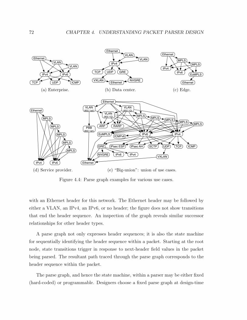
72 CHAPTER 4. UNDERSTANDING PACKET PARSER DESIGN
EthernetVLAN
VLAN
IPv4 IPv6
TCP UDP ICMP
(a) Enterprise.
EthernetVLAN
VLANIPv4
GRE
NVGREEthernet
TCP UDP
VXLAN
(b) Data center.
Ethernet
IPv4
MPLS
IPv6
MPLS
EoMPLS
Ethernet
(c) Edge.
Ethernet
IPv4 IPv6
MPLS
MPLS
MPLS
MPLS
MPLS
(d) Service provider.
Ethernet
IPv4
VLAN(802.1Q)
VLAN(802.1Q) MPLS MPLS MPLS MPLS MPLS
IPv6
ARP RARP
VLAN(802.1ad)
PBB(802.1ah)
Ethernet
EoMPLS
ICMP
ICMPv6
TCPUDPGRE IPsec ESP IPsec AH SCTP
VXLANNVGRE IPv4IPv6
(e) “Big-union”: union of use cases.
Figure 4.4: Parse graph examples for various use cases.
with an Ethernet header for this network. The Ethernet header may be followed by
either a VLAN, an IPv4, an IPv6, or no header; the figure does not show transitions
that end the header sequence. An inspection of the graph reveals similar successor
relationships for other header types.
A parse graph not only expresses header sequences; it is also the state machine
for sequentially identifying the header sequence within a packet. Starting at the root
node, state transitions trigger in response to next-header field values in the packet
being parsed. The resultant path traced through the parse graph corresponds to the
header sequence within the packet.
The parse graph, and hence the state machine, within a parser may be either fixed
(hard-coded) or programmable. Designers choose a fixed parse graph at design-time
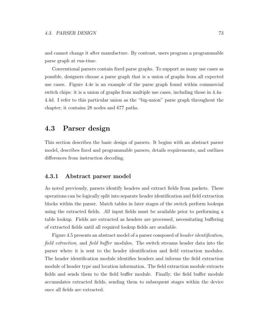
4.3. PARSER DESIGN 73
and cannot change it after manufacture. By contrast, users program a programmable
parse graph at run-time.
Conventional parsers contain fixed parse graphs. To support as many use cases as
possible, designers choose a parse graph that is a union of graphs from all expected
use cases. Figure 4.4e is an example of the parse graph found within commercial
switch chips: it is a union of graphs from multiple use cases, including those in 4.4a–
4.4d. I refer to this particular union as the “big-union” parse graph throughout the
chapter; it contains 28 nodes and 677 paths.
4.3 Parser design
This section describes the basic design of parsers. It begins with an abstract parser
model, describes fixed and programmable parsers, details requirements, and outlines
differences from instruction decoding.
4.3.1 Abstract parser model
As noted previously, parsers identify headers and extract fields from packets. These
operations can be logically split into separate header identification and field extraction
blocks within the parser. Match tables in later stages of the switch perform lookups
using the extracted fields. All input fields must be available prior to performing a
table lookup. Fields are extracted as headers are processed, necessitating buffering
of extracted fields until all required lookup fields are available.
Figure 4.5 presents an abstract model of a parser composed of header identification,
field extraction, and field buffer modules. The switch streams header data into the
parser where it is sent to the header identification and field extraction modules.
The header identification module identifies headers and informs the field extraction
module of header type and location information. The field extraction module extracts
fields and sends them to the field buffer module. Finally, the field buffer module
accumulates extracted fields, sending them to subsequent stages within the device
once all fields are extracted.
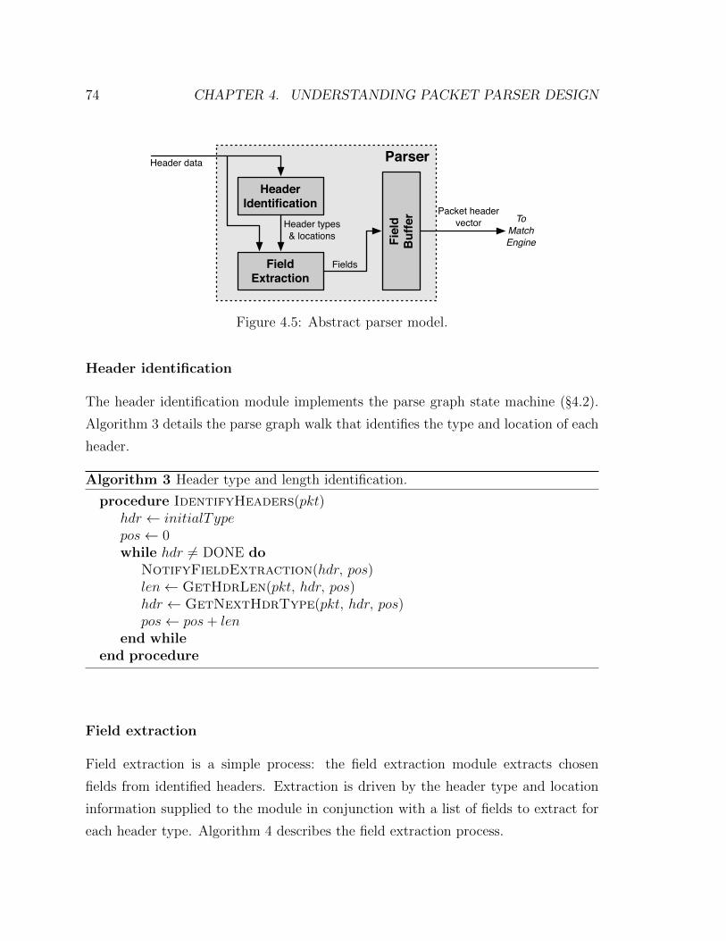
74 CHAPTER 4. UNDERSTANDING PACKET PARSER DESIGN
ParserHeader data
Header Identification
Field Extraction
Fields
Fiel
dB
uffe
r Packet headervector To
MatchEngine
Header types& locations
Figure 4.5: Abstract parser model.
Header identification
The header identification module implements the parse graph state machine (§4.2).
Algorithm 3 details the parse graph walk that identifies the type and location of each
header.
Algorithm 3 Header type and length identification.
procedure IdentifyHeaders(pkt)hdr ← initialTypepos← 0while hdr 6= DONE do
NotifyFieldExtraction(hdr, pos)len← GetHdrLen(pkt, hdr, pos)hdr ← GetNextHdrType(pkt, hdr, pos)pos← pos+ len
end whileend procedure
Field extraction
Field extraction is a simple process: the field extraction module extracts chosen
fields from identified headers. Extraction is driven by the header type and location
information supplied to the module in conjunction with a list of fields to extract for
each header type. Algorithm 4 describes the field extraction process.

4.3. PARSER DESIGN 75
Algorithm 4 Field extraction.
procedure ExtractFields(pkt, hdr, hdrPos)fields← GetFieldList(hdr)for (fieldPos, fieldLen)← fields do
Extract(pkt, hdrPos+ fieldPos, fieldLen)end for
end procedure
Field extraction may occur in parallel with header identification: the field ex-
traction module extracts fields from identified regions while the header identification
module identifies unprocessed regions. No serial dependency exists between headers
once the header identification module resolves the type and location, allowing the
extraction of multiple fields from multiple headers in parallel.
Field buffer
The field buffer accumulates extracted fields prior to table lookups by the switch.
Extracted fields are output as a wide bit vector by the buffer because table lookups
match on all fields in parallel. Outputting a wide bit vector requires the buffer to be
implemented as a wide array of registers. One multiplexor is required per register to
select between each field output from the field extraction block.
4.3.2 Fixed parser
A fixed parser processes a single parse graph chosen at design-time. The chosen
parse graph is a union of the parse graphs for each use case the switch is designed
to support. Designers optimize the logic within a fixed parser for the chosen parse
graph.
I have presented a design that may not precisely match the parser within any par-
ticular commercial switch, but is qualitatively representative of commercial parsers.
As shown in §4.5.2, the area of a fixed parser is dominated by the field buffer. The
width of this buffer is determined by the parse graph, and the need to send all ex-
tracted fields in parallel to the downstream match engine requires it be constructed
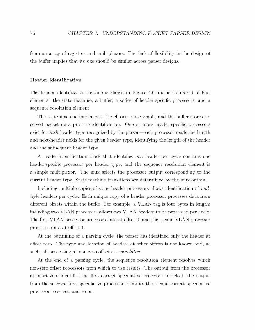
76 CHAPTER 4. UNDERSTANDING PACKET PARSER DESIGN
from an array of registers and multiplexors. The lack of flexibility in the design of
the buffer implies that its size should be similar across parser designs.
Header identification
The header identification module is shown in Figure 4.6 and is composed of four
elements: the state machine, a buffer, a series of header-specific processors, and a
sequence resolution element.
The state machine implements the chosen parse graph, and the buffer stores re-
ceived packet data prior to identification. One or more header-specific processors
exist for each header type recognized by the parser—each processor reads the length
and next-header fields for the given header type, identifying the length of the header
and the subsequent header type.
A header identification block that identifies one header per cycle contains one
header-specific processor per header type, and the sequence resolution element is
a simple multiplexor. The mux selects the processor output corresponding to the
current header type. State machine transitions are determined by the mux output.
Including multiple copies of some header processors allows identification of mul-
tiple headers per cycle. Each unique copy of a header processor processes data from
different offsets within the buffer. For example, a VLAN tag is four bytes in length;
including two VLAN processors allows two VLAN headers to be processed per cycle.
The first VLAN processor processes data at offset 0, and the second VLAN processor
processes data at offset 4.
At the beginning of a parsing cycle, the parser has identified only the header at
offset zero. The type and location of headers at other offsets is not known and, as
such, all processing at non-zero offsets is speculative.
At the end of a parsing cycle, the sequence resolution element resolves which
non-zero offset processors from which to use results. The output from the processor
at offset zero identifies the first correct speculative processor to select, the output
from the selected first speculative processor identifies the second correct speculative
processor to select, and so on.
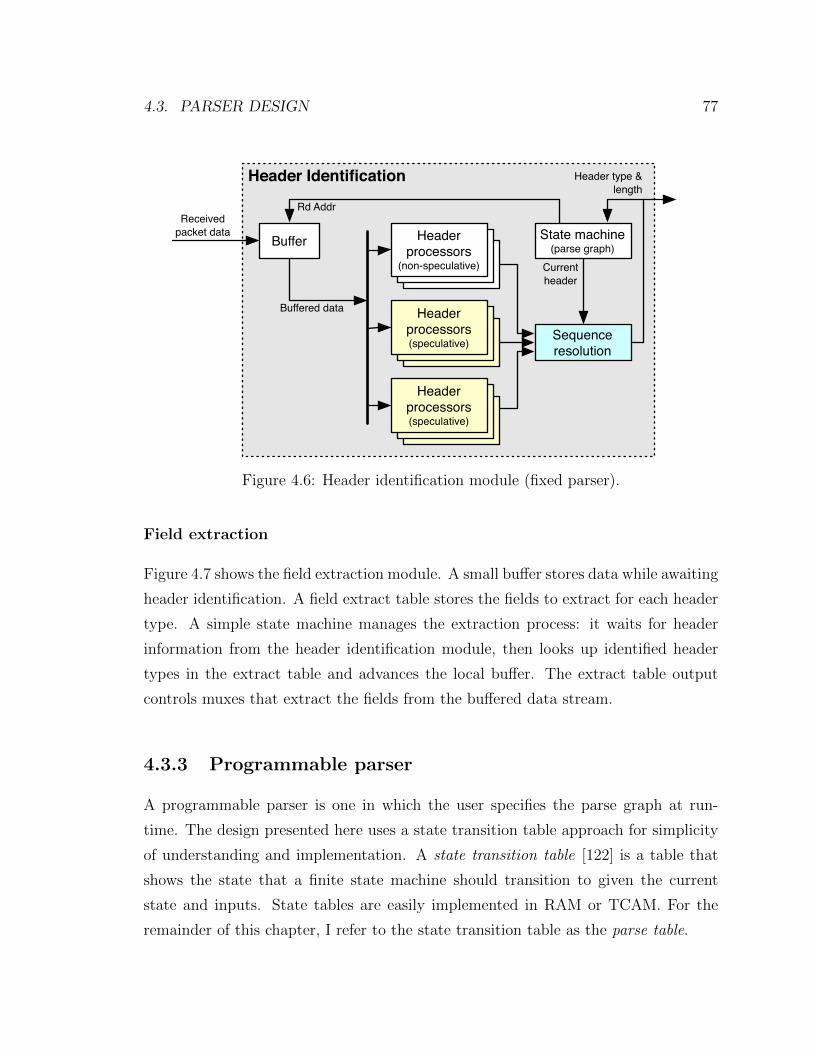
4.3. PARSER DESIGN 77
Header Identification
Sequence resolution
Buffer State machine(parse graph)
Header processors
(non-speculative)
Receivedpacket data
Rd Addr
Buffered data
Header type & length
Header processors(speculative)
Header processors(speculative)
Currentheader
Figure 4.6: Header identification module (fixed parser).
Field extraction
Figure 4.7 shows the field extraction module. A small buffer stores data while awaiting
header identification. A field extract table stores the fields to extract for each header
type. A simple state machine manages the extraction process: it waits for header
information from the header identification module, then looks up identified header
types in the extract table and advances the local buffer. The extract table output
controls muxes that extract the fields from the buffered data stream.
4.3.3 Programmable parser
A programmable parser is one in which the user specifies the parse graph at run-
time. The design presented here uses a state transition table approach for simplicity
of understanding and implementation. A state transition table [122] is a table that
shows the state that a finite state machine should transition to given the current
state and inputs. State tables are easily implemented in RAM or TCAM. For the
remainder of this chapter, I refer to the state transition table as the parse table.
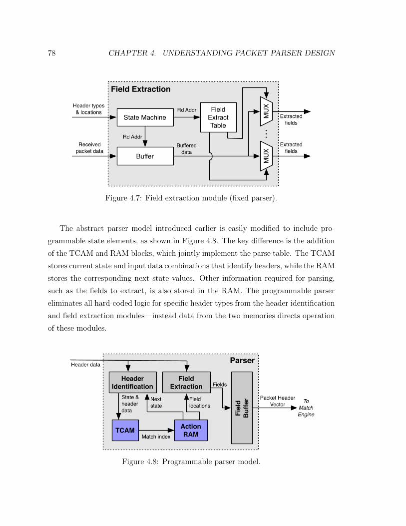
78 CHAPTER 4. UNDERSTANDING PACKET PARSER DESIGN
Field Extraction
Buffer
State Machine
Receivedpacket data
Rd AddrBuffered
data
Field Extract Table
MU
XM
UX
⋮
Rd AddrHeader types& locations
Extractedfields
Extractedfields
Figure 4.7: Field extraction module (fixed parser).
The abstract parser model introduced earlier is easily modified to include pro-
grammable state elements, as shown in Figure 4.8. The key difference is the addition
of the TCAM and RAM blocks, which jointly implement the parse table. The TCAM
stores current state and input data combinations that identify headers, while the RAM
stores the corresponding next state values. Other information required for parsing,
such as the fields to extract, is also stored in the RAM. The programmable parser
eliminates all hard-coded logic for specific header types from the header identification
and field extraction modules—instead data from the two memories directs operation
of these modules.
Parser
TCAM Action RAM
Header Identification
Field Extraction Fields
Fiel
dB
uffe
r
Header data
Packet HeaderVector To
MatchEngine
Nextstate
State &headerdata
Match index
Fieldlocations
Figure 4.8: Programmable parser model.
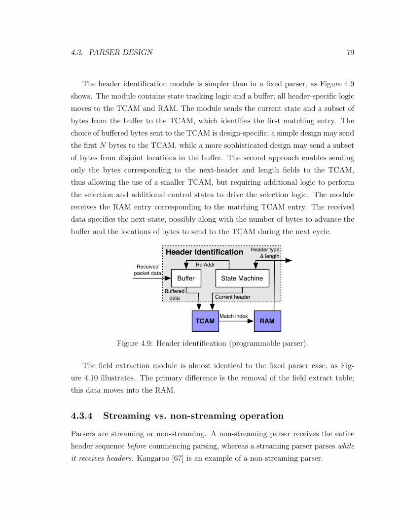
4.3. PARSER DESIGN 79
The header identification module is simpler than in a fixed parser, as Figure 4.9
shows. The module contains state tracking logic and a buffer; all header-specific logic
moves to the TCAM and RAM. The module sends the current state and a subset of
bytes from the buffer to the TCAM, which identifies the first matching entry. The
choice of buffered bytes sent to the TCAM is design-specific; a simple design may send
the first N bytes to the TCAM, while a more sophisticated design may send a subset
of bytes from disjoint locations in the buffer. The second approach enables sending
only the bytes corresponding to the next-header and length fields to the TCAM,
thus allowing the use of a smaller TCAM, but requiring additional logic to perform
the selection and additional control states to drive the selection logic. The module
receives the RAM entry corresponding to the matching TCAM entry. The received
data specifies the next state, possibly along with the number of bytes to advance the
buffer and the locations of bytes to send to the TCAM during the next cycle.
Header Identification
Buffer State Machine
Receivedpacket data
Rd Addr
Buffereddata
TCAM RAM
Current header
Match index
Header type& length
Figure 4.9: Header identification (programmable parser).
The field extraction module is almost identical to the fixed parser case, as Fig-
ure 4.10 illustrates. The primary difference is the removal of the field extract table;
this data moves into the RAM.
4.3.4 Streaming vs. non-streaming operation
Parsers are streaming or non-streaming. A non-streaming parser receives the entire
header sequence before commencing parsing, whereas a streaming parser parses while
it receives headers. Kangaroo [67] is an example of a non-streaming parser.
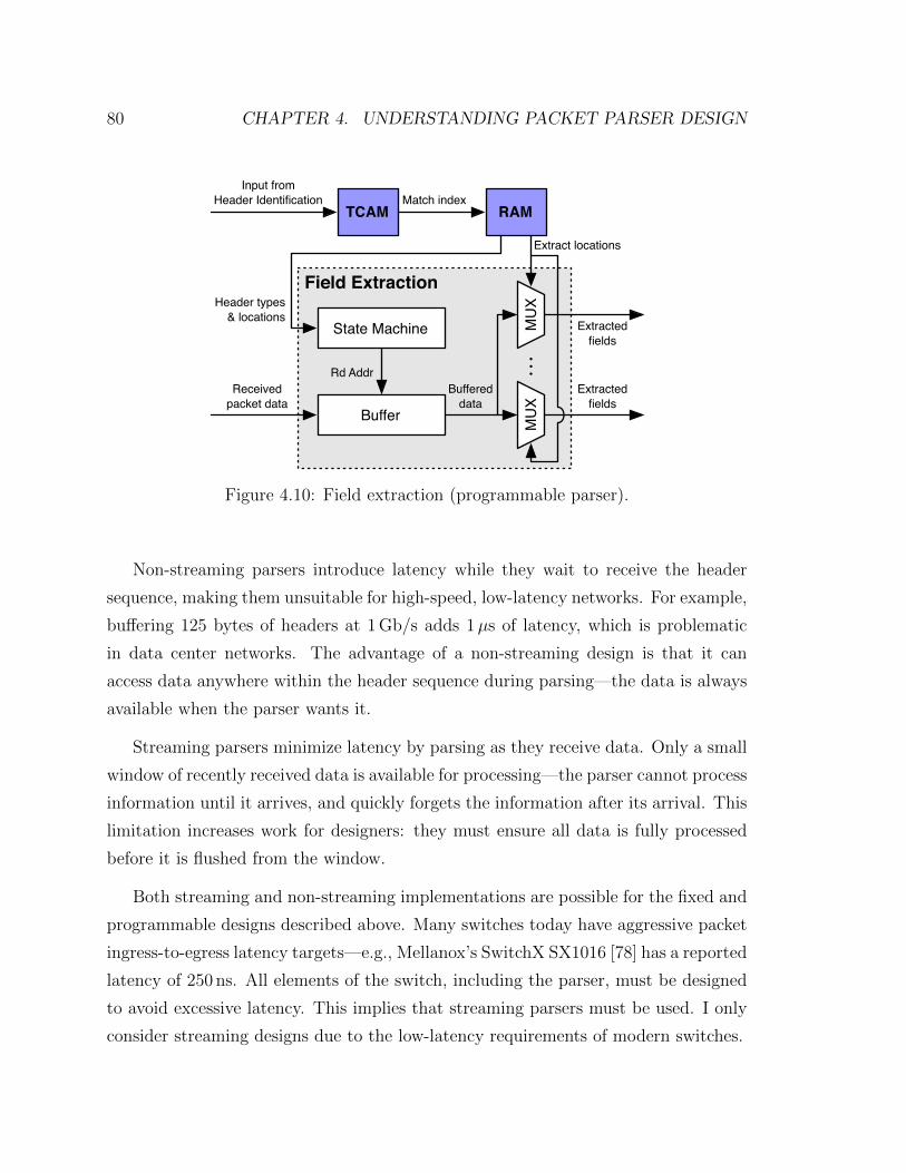
80 CHAPTER 4. UNDERSTANDING PACKET PARSER DESIGN
Field Extraction
TCAM RAM
Input fromHeader Identification
Buffer
State Machine
Receivedpacket data
Rd AddrBuffered
data
⋮
Header types& locations
Match index
Extract locations
Extractedfields
Extractedfields
MU
XM
UX
Figure 4.10: Field extraction (programmable parser).
Non-streaming parsers introduce latency while they wait to receive the header
sequence, making them unsuitable for high-speed, low-latency networks. For example,
buffering 125 bytes of headers at 1 Gb/s adds 1µs of latency, which is problematic
in data center networks. The advantage of a non-streaming design is that it can
access data anywhere within the header sequence during parsing—the data is always
available when the parser wants it.
Streaming parsers minimize latency by parsing as they receive data. Only a small
window of recently received data is available for processing—the parser cannot process
information until it arrives, and quickly forgets the information after its arrival. This
limitation increases work for designers: they must ensure all data is fully processed
before it is flushed from the window.
Both streaming and non-streaming implementations are possible for the fixed and
programmable designs described above. Many switches today have aggressive packet
ingress-to-egress latency targets—e.g., Mellanox’s SwitchX SX1016 [78] has a reported
latency of 250 ns. All elements of the switch, including the parser, must be designed
to avoid excessive latency. This implies that streaming parsers must be used. I only
consider streaming designs due to the low-latency requirements of modern switches.
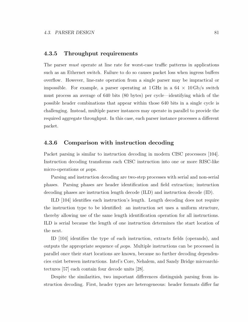
4.3. PARSER DESIGN 81
4.3.5 Throughput requirements
The parser must operate at line rate for worst-case traffic patterns in applications
such as an Ethernet switch. Failure to do so causes packet loss when ingress buffers
overflow. However, line-rate operation from a single parser may be impractical or
impossible. For example, a parser operating at 1 GHz in a 64 × 10 Gb/s switch
must process an average of 640 bits (80 bytes) per cycle—identifying which of the
possible header combinations that appear within those 640 bits in a single cycle is
challenging. Instead, multiple parser instances may operate in parallel to provide the
required aggregate throughput. In this case, each parser instance processes a different
packet.
4.3.6 Comparison with instruction decoding
Packet parsing is similar to instruction decoding in modern CISC processors [104].
Instruction decoding transforms each CISC instruction into one or more RISC-like
micro-operations or µops.
Parsing and instruction decoding are two-step processes with serial and non-serial
phases. Parsing phases are header identification and field extraction; instruction
decoding phases are instruction length decode (ILD) and instruction decode (ID).
ILD [104] identifies each instruction’s length. Length decoding does not require
the instruction type to be identified: an instruction set uses a uniform structure,
thereby allowing use of the same length identification operation for all instructions.
ILD is serial because the length of one instruction determines the start location of
the next.
ID [104] identifies the type of each instruction, extracts fields (operands), and
outputs the appropriate sequence of µops. Multiple instructions can be processed in
parallel once their start locations are known, because no further decoding dependen-
cies exist between instructions. Intel’s Core, Nehalem, and Sandy Bridge microarchi-
tectures [57] each contain four decode units [28].
Despite the similarities, two important differences distinguish parsing from in-
struction decoding. First, header types are heterogeneous: header formats differ far

82 CHAPTER 4. UNDERSTANDING PACKET PARSER DESIGN
more than instruction formats. Second, headers contain insufficient information to
identify their type uniquely unlike instructions; a header’s type is identified by the
next-header field in the preceding header.
4.4 Parse table generation
A discussion of programmable parsers is incomplete without consideration of parse
table entry generation. This section describes parse table entries and presents an
algorithm and heuristics for minimizing the number of entries.
4.4.1 Parse table structure
The parse table is a state transition table. As the name implies, a state transition
table specifies the transitions between states in a state machine. A state transition
table contains columns for the current state, the input value(s), the next state, and
any output value(s). Each table row specifies the state to transition to for a specific
current state and input value combination. A row exists for each valid state and input
value combination.
The parse table columns are the current header type, the packet data lookup
values, the next header type, the current header length, and the lookup offsets for
use in the next cycle. Every edge in the parse graph is a state transition, therefore
a parse table entry must encode every edge. Figure 4.11a shows a section of a parse
graph, and Figure 4.11b shows the corresponding parse table entries.
VLAN1
VLAN2IPv4
(a) Parse graph fragment.
Curr. Hdr. Lookup Val. Next Hdr.VLAN1 0x0800 IPv4VLAN1 0x8100 VLAN2
VLAN1 ANY —VLAN2 0x0800 IPv4VLAN2 ANY —
(b) Corresponding parse table entries.
Figure 4.11: Sample parse table entries.

4.4. PARSE TABLE GENERATION 83
Only fields that convey useful information need to be input to the parse table.
Important fields for header identification are the current header length and the next
header type fields.
Unfortunately, the useful fields reside at different locations in different header
types. Two mechanisms are required to send a subset of data to the parse table: one
to indicate which fields to send, and another to extract the useful fields. The lookup
offsets encoded in the parse table indicate the words within the buffered packet data
to send to the parse table in the next cycle. Multiplexors extract the selected data
from the buffer.
Sending only a subset of data to the parse table reduces the table size—e.g., the
parse table requires only four bytes of the 20+ bytes in an IPv4 header. A naıve
implementation that sends each consecutive packet word to a 32 bit wide TCAM—
used to match eight bits of state and 32 bits of packet data—requires 342 entries, or
13,680 b, to implement the big-union parse graph. Sending only the data needed to
identify header types and lengths to the TCAM, in conjunction with the optimizations
detailed below, reduces the requirement to 112 entries or 4,480 b. This optimized
implementation reduces the number of TCAM entries by a factor of three.
4.4.2 Efficient table generation
A single entry may encode multiple transitions. This has two benefits: it can reduce
the total number of table entries, and it allows a single parsing cycle to identify
multiple headers. Figure 4.12a encodes the parse graph fragment of Figure 4.11a
using entries with multiple transitions. This new table contains one less entry than
the table in Figure 4.11b. Because the parse table is one of two main contributors to
area (§4.5.3), minimizing the entry count reduces the parser’s area.
Combining multiple transitions within a table entry is node clustering or merging.
The first two entries in Figure 4.12a process two VLAN tags simultaneously: the
first lookup value processes VLAN1’s next header field and the second lookup value
processes VLAN2’s next header field. The cluster corresponding to the first two
entries is shown in Figure 4.12b.
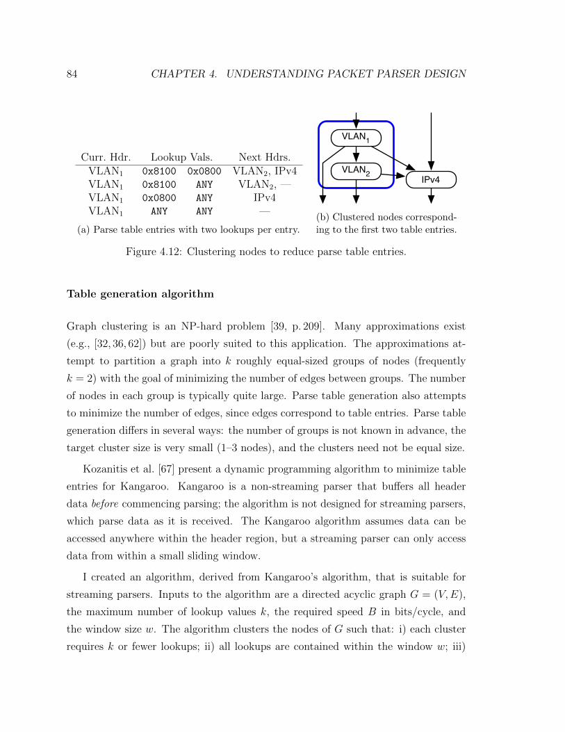
84 CHAPTER 4. UNDERSTANDING PACKET PARSER DESIGN
Curr. Hdr. Lookup Vals. Next Hdrs.VLAN1 0x8100 0x0800 VLAN2, IPv4VLAN1 0x8100 ANY VLAN2, —VLAN1 0x0800 ANY IPv4VLAN1 ANY ANY —
(a) Parse table entries with two lookups per entry.
VLAN1
VLAN2IPv4
(b) Clustered nodes correspond-ing to the first two table entries.
Figure 4.12: Clustering nodes to reduce parse table entries.
Table generation algorithm
Graph clustering is an NP-hard problem [39, p. 209]. Many approximations exist
(e.g., [32, 36, 62]) but are poorly suited to this application. The approximations at-
tempt to partition a graph into k roughly equal-sized groups of nodes (frequently
k = 2) with the goal of minimizing the number of edges between groups. The number
of nodes in each group is typically quite large. Parse table generation also attempts
to minimize the number of edges, since edges correspond to table entries. Parse table
generation differs in several ways: the number of groups is not known in advance, the
target cluster size is very small (1–3 nodes), and the clusters need not be equal size.
Kozanitis et al. [67] present a dynamic programming algorithm to minimize table
entries for Kangaroo. Kangaroo is a non-streaming parser that buffers all header
data before commencing parsing; the algorithm is not designed for streaming parsers,
which parse data as it is received. The Kangaroo algorithm assumes data can be
accessed anywhere within the header region, but a streaming parser can only access
data from within a small sliding window.
I created an algorithm, derived from Kangaroo’s algorithm, that is suitable for
streaming parsers. Inputs to the algorithm are a directed acyclic graph G = (V,E),
the maximum number of lookup values k, the required speed B in bits/cycle, and
the window size w. The algorithm clusters the nodes of G such that: i) each cluster
requires k or fewer lookups; ii) all lookups are contained within the window w; iii)
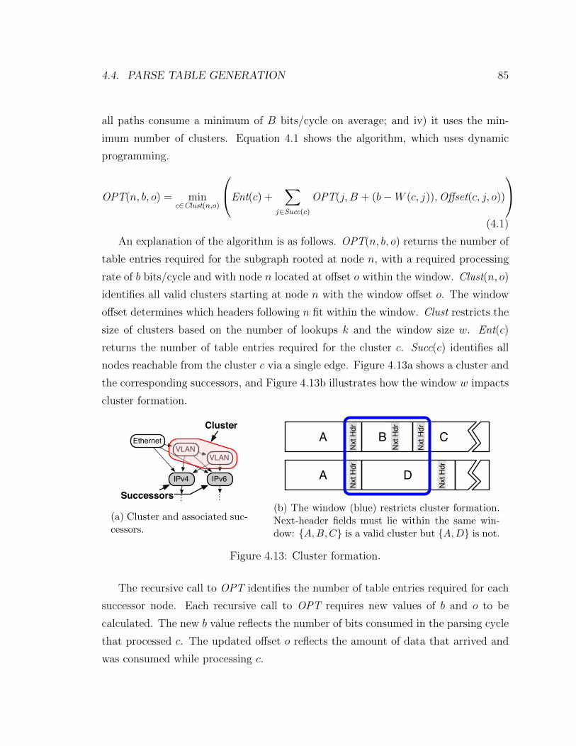
4.4. PARSE TABLE GENERATION 85
all paths consume a minimum of B bits/cycle on average; and iv) it uses the min-
imum number of clusters. Equation 4.1 shows the algorithm, which uses dynamic
programming.
OPT(n, b, o) = minc∈Clust(n,o)
Ent(c) +∑
j∈Succ(c)
OPT(j, B + (b−W (c, j)),Offset(c, j, o))
(4.1)
An explanation of the algorithm is as follows. OPT(n, b, o) returns the number of
table entries required for the subgraph rooted at node n, with a required processing
rate of b bits/cycle and with node n located at offset o within the window. Clust(n, o)
identifies all valid clusters starting at node n with the window offset o. The window
offset determines which headers following n fit within the window. Clust restricts the
size of clusters based on the number of lookups k and the window size w. Ent(c)
returns the number of table entries required for the cluster c. Succ(c) identifies all
nodes reachable from the cluster c via a single edge. Figure 4.13a shows a cluster and
the corresponding successors, and Figure 4.13b illustrates how the window w impacts
cluster formation.
EthernetVLAN
VLAN
IPv4 IPv6
⋮ ⋮
Cluster
Successors
(a) Cluster and associated suc-cessors.
Nxt
Hdr
Nxt
Hdr
C
Nxt
Hdr
AN
xt H
dr
Nxt
Hdr
A D
B
(b) The window (blue) restricts cluster formation.Next-header fields must lie within the same win-dow: {A,B,C} is a valid cluster but {A,D} is not.
Figure 4.13: Cluster formation.
The recursive call to OPT identifies the number of table entries required for each
successor node. Each recursive call to OPT requires new values of b and o to be
calculated. The new b value reflects the number of bits consumed in the parsing cycle
that processed c. The updated offset o reflects the amount of data that arrived and
was consumed while processing c.
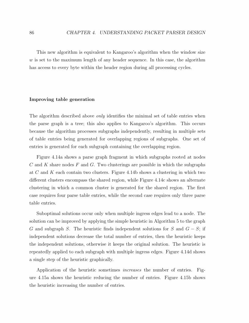
86 CHAPTER 4. UNDERSTANDING PACKET PARSER DESIGN
This new algorithm is equivalent to Kangaroo’s algorithm when the window size
w is set to the maximum length of any header sequence. In this case, the algorithm
has access to every byte within the header region during all processing cycles.
Improving table generation
The algorithm described above only identifies the minimal set of table entries when
the parse graph is a tree; this also applies to Kangaroo’s algorithm. This occurs
because the algorithm processes subgraphs independently, resulting in multiple sets
of table entries being generated for overlapping regions of subgraphs. One set of
entries is generated for each subgraph containing the overlapping region.
Figure 4.14a shows a parse graph fragment in which subgraphs rooted at nodes
C and K share nodes F and G. Two clusterings are possible in which the subgraphs
at C and K each contain two clusters. Figure 4.14b shows a clustering in which two
different clusters encompass the shared region, while Figure 4.14c shows an alternate
clustering in which a common cluster is generated for the shared region. The first
case requires four parse table entries, while the second case requires only three parse
table entries.
Suboptimal solutions occur only when multiple ingress edges lead to a node. The
solution can be improved by applying the simple heuristic in Algorithm 5 to the graph
G and subgraph S. The heuristic finds independent solutions for S and G − S; if
independent solutions decrease the total number of entries, then the heuristic keeps
the independent solutions, otherwise it keeps the original solution. The heuristic is
repeatedly applied to each subgraph with multiple ingress edges. Figure 4.14d shows
a single step of the heuristic graphically.
Application of the heuristic sometimes increases the number of entries. Fig-
ure 4.15a shows the heuristic reducing the number of entries. Figure 4.15b shows
the heuristic increasing the number of entries.

4.4. PARSE TABLE GENERATION 87
......
C
D
EF
G
K
L
M
(a) Parse graph fragmentwith shared nodes F and G.
......
C
D
EF
G
K
L
M
(b) Multiple clusters con-tain nodes F and G.
......
C
D
EF
G
K
L
M
(c) A clustering with F andG in one cluster.
Remove and solveindependently
(d) Remove and solve subgraphs with multiple parentsindependently to prevent nodes appearing in multipleclusters.
Figure 4.14: Improving cluster formation.
Algorithm 5 Heuristic to improve table generation for shared subgraphs.
function ImproveSharedSubgraph(G, S)Eorig = Opt(G) . Find solutions for G, S, and G− S.Esub = Opt(S)Ediff = Opt(G− S)
if Count(Esub) + Count(Ediff) < Count(Eorig) thenreturn (G− S, S) . S removed; use G− S in subsequent steps.
elsereturn (G, []) . Nothing removed; use G in subsequent steps.
end ifend function
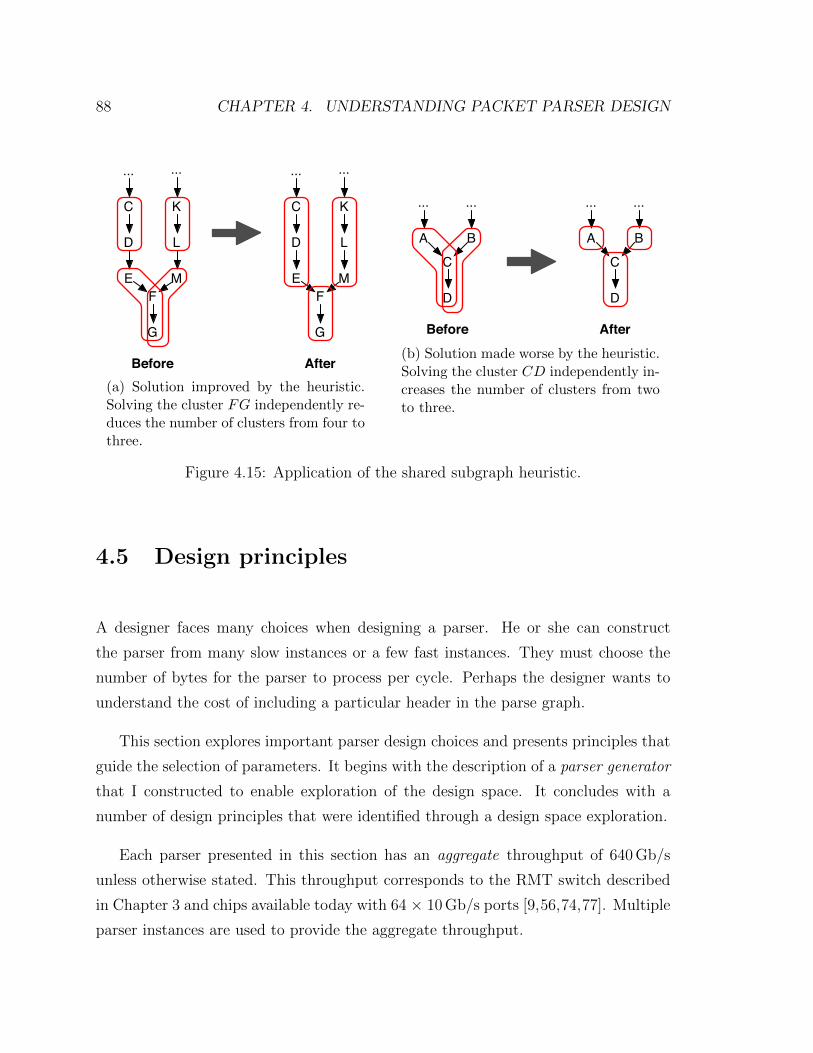
88 CHAPTER 4. UNDERSTANDING PACKET PARSER DESIGN
Before After
......
C
D
EF
G
K
L
M
......
C
D
EF
G
K
L
M
(a) Solution improved by the heuristic.Solving the cluster FG independently re-duces the number of clusters from four tothree.
Before After
...
A
C
D
...
B
...
A
C
D
...
B
(b) Solution made worse by the heuristic.Solving the cluster CD independently in-creases the number of clusters from twoto three.
Figure 4.15: Application of the shared subgraph heuristic.
4.5 Design principles
A designer faces many choices when designing a parser. He or she can construct
the parser from many slow instances or a few fast instances. They must choose the
number of bytes for the parser to process per cycle. Perhaps the designer wants to
understand the cost of including a particular header in the parse graph.
This section explores important parser design choices and presents principles that
guide the selection of parameters. It begins with the description of a parser generator
that I constructed to enable exploration of the design space. It concludes with a
number of design principles that were identified through a design space exploration.
Each parser presented in this section has an aggregate throughput of 640 Gb/s
unless otherwise stated. This throughput corresponds to the RMT switch described
in Chapter 3 and chips available today with 64 × 10 Gb/s ports [9,56,74,77]. Multiple
parser instances are used to provide the aggregate throughput.

4.5. DESIGN PRINCIPLES 89
4.5.1 Parser generator
A thorough exploration of the design space requires the analysis and comparison of
many unique parser instances. To facilitate this, I built a parser generator that gener-
ates unique parser instances for user-supplied parse graphs and associated parameter
sets.
I built the parser generator atop the Genesis [103] chip generator. Genesis is a
tool that generates design instances using an architectural “template” and a set of
application configuration parameters. Templates consist of a mix of Verilog and Perl;
the Verilog expresses the logic being generated, and the Perl codifies design choices
to enable programmatic generation of Verilog code.
The parser generator generates fixed and programmable parsers, as described in
§4.3.2 and §4.3.3. Parameters controlling generation include the parse graph, the
processing width, the parser type (fixed/programmable), the field buffer depth, and
the size of the programmable TCAM/RAM. The generator outputs synthesizable
Verilog. I produced all the reported area and power results using Synopsys Design
Compiler G-2012.06 and a 45 nm TSMC library.
The parser generator is available for download from http://yuba.stanford.edu/
~grg/parser.html
Generator operation
Fixed parsers: A fixed parser supports a single parse graph chosen at design-time.
Two parameters are primarily responsible for guiding generation of a fixed parser:
the parse graph and the processing width. The parse graph specifies the headers sup-
ported by the parser and their orderings; the processing width specifies the quantity
of data input to the parser each clock cycle.
The designer specifies the parse graph in a text file containing a description of
each header type. For each header type, the description contains the name and size
of all fields, a list of which fields to extract, a mapping between field values and next
header types. For variable-length headers, the description also includes a mapping
that identifies header length from field values.
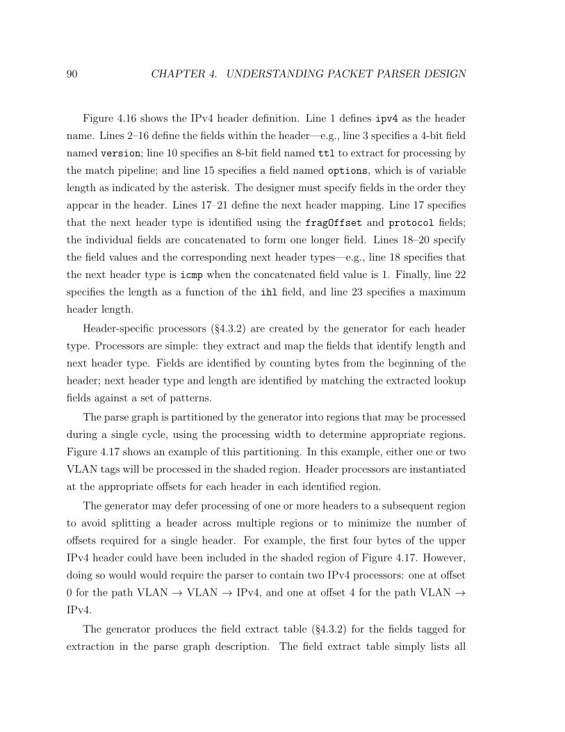
90 CHAPTER 4. UNDERSTANDING PACKET PARSER DESIGN
Figure 4.16 shows the IPv4 header definition. Line 1 defines ipv4 as the header
name. Lines 2–16 define the fields within the header—e.g., line 3 specifies a 4-bit field
named version; line 10 specifies an 8-bit field named ttl to extract for processing by
the match pipeline; and line 15 specifies a field named options, which is of variable
length as indicated by the asterisk. The designer must specify fields in the order they
appear in the header. Lines 17–21 define the next header mapping. Line 17 specifies
that the next header type is identified using the fragOffset and protocol fields;
the individual fields are concatenated to form one longer field. Lines 18–20 specify
the field values and the corresponding next header types—e.g., line 18 specifies that
the next header type is icmp when the concatenated field value is 1. Finally, line 22
specifies the length as a function of the ihl field, and line 23 specifies a maximum
header length.
Header-specific processors (§4.3.2) are created by the generator for each header
type. Processors are simple: they extract and map the fields that identify length and
next header type. Fields are identified by counting bytes from the beginning of the
header; next header type and length are identified by matching the extracted lookup
fields against a set of patterns.
The parse graph is partitioned by the generator into regions that may be processed
during a single cycle, using the processing width to determine appropriate regions.
Figure 4.17 shows an example of this partitioning. In this example, either one or two
VLAN tags will be processed in the shaded region. Header processors are instantiated
at the appropriate offsets for each header in each identified region.
The generator may defer processing of one or more headers to a subsequent region
to avoid splitting a header across multiple regions or to minimize the number of
offsets required for a single header. For example, the first four bytes of the upper
IPv4 header could have been included in the shaded region of Figure 4.17. However,
doing so would would require the parser to contain two IPv4 processors: one at offset
0 for the path VLAN → VLAN → IPv4, and one at offset 4 for the path VLAN →IPv4.
The generator produces the field extract table (§4.3.2) for the fields tagged for
extraction in the parse graph description. The field extract table simply lists all
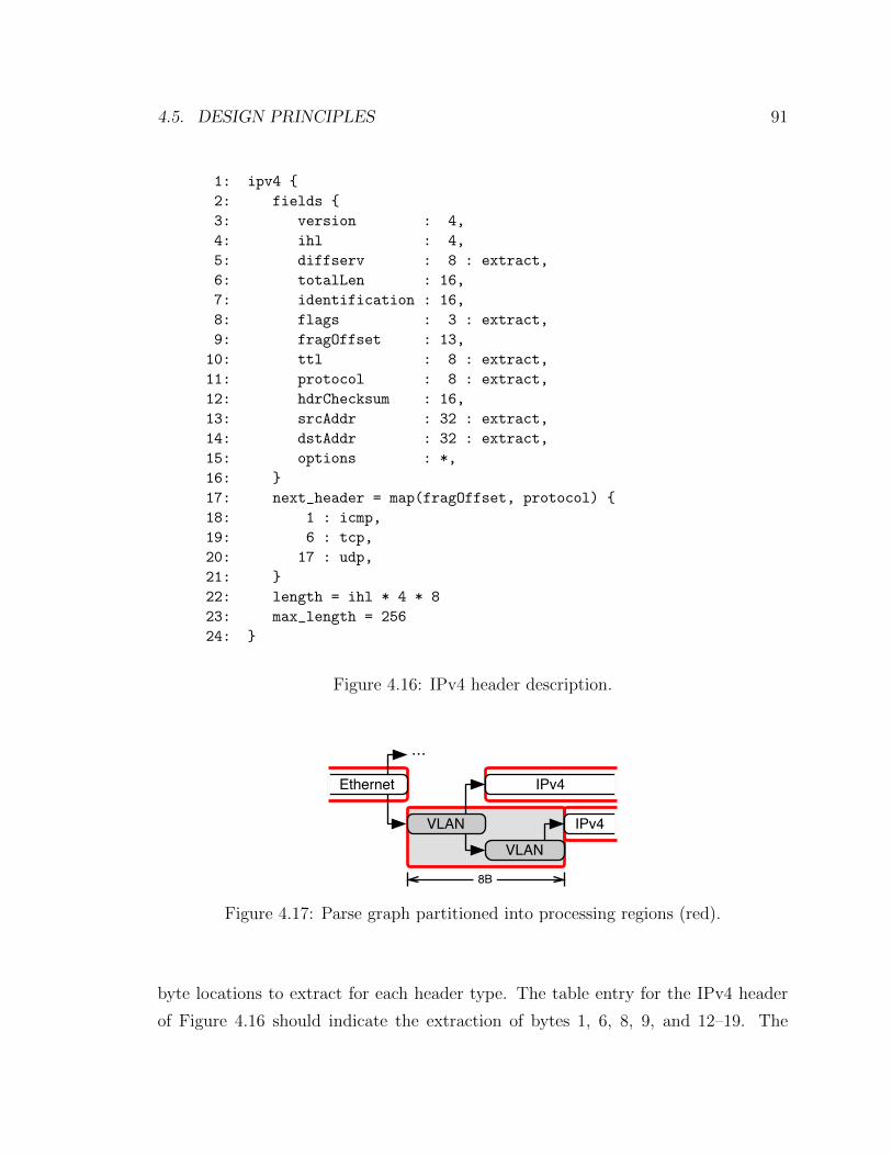
4.5. DESIGN PRINCIPLES 91
1: ipv4 {
2: fields {
3: version : 4,
4: ihl : 4,
5: diffserv : 8 : extract,
6: totalLen : 16,
7: identification : 16,
8: flags : 3 : extract,
9: fragOffset : 13,
10: ttl : 8 : extract,
11: protocol : 8 : extract,
12: hdrChecksum : 16,
13: srcAddr : 32 : extract,
14: dstAddr : 32 : extract,
15: options : *,
16: }
17: next_header = map(fragOffset, protocol) {
18: 1 : icmp,
19: 6 : tcp,
20: 17 : udp,
21: }
22: length = ihl * 4 * 8
23: max_length = 256
24: }
Figure 4.16: IPv4 header description.
VLAN
VLAN
�
Ethernet
IPv4
IPv4
8B
Figure 4.17: Parse graph partitioned into processing regions (red).
byte locations to extract for each header type. The table entry for the IPv4 header
of Figure 4.16 should indicate the extraction of bytes 1, 6, 8, 9, and 12–19. The
92 CHAPTER 4. UNDERSTANDING PACKET PARSER DESIGN
generator sizes the field buffer automatically for the fixed parser to accommodate all
fields requiring extraction.
Programmable parser: A programmable parser allows the user to specify the
parse graph at chip run-time rather than design-time. Parameters that are important
to the generation of a programmable parser include the processing width, the parse
table dimensions, the window size, and the number and size of parse table lookups.
A parse graph is not required to generate a programmable parser, because the user
specifies the graph at run-time, but the generator uses a parse graph to generate a
test bench (see below).
The generator uses the parameters to determine component sizes and counts. For
example, the window size determines the input buffer depth within the header identi-
fication component and the number of multiplexor inputs needed for field extraction
prior to lookup in the parse table. Similarly, the number of parse table inputs deter-
mines the number of multiplexors required to extract inputs. Unlike the fixed parser,
the programmable parser does not contain any logic specific to a particular parse
graph.
The generator does not generate the TCAM and RAM used by the parse table. A
vendor-supplied memory generator must generate memories for the process technology
in use. The parser generator produces non-synthesizable models for use in simulation.
Test bench: The generator outputs a test bench to verify each parser it generates.
The test bench transmits a number of packets to the parser and verifies that the parser
identifies and extracts the correct set of header fields for each input packet. The
generator creates input packets for the parse graph input to the generator, and the
processing width parameter determines the input width of the packet byte sequences.
In the case of a programmable parser, the test bench initializes the TCAM and RAM
with the contents of the parse table.
4.5.2 Fixed parser design principles
The design space exploration revealed that relatively few design choices make any
appreciable impact on the resultant parser—most design choices have a small impact
4.5. DESIGN PRINCIPLES 93
on properties such as size and power. This section details the main principles that
apply to fixed parser design.
Principle: The processing width of a single parser instance trades area for
power.
A single parser instance’s throughput is r = w×f , where r is the rate or throughput,
w is the processing width, and f is the clock frequency. If the parser throughput is
fixed, then w ∝ 1/f.
Figure 4.18a shows the area and power of a single parser instance with a through-
put of 10 Gb/s. Parser area increases as processing width increases, because addi-
tional resources are required to process the additional data. Additional resources are
required for two reasons. First, the packet data bus increases in width, requiring more
wires, registers, multiplexors, and so on. Second, additional headers can occur within
a single processing region (§4.5.1), requiring more header-specific processor instances.
Power consumption decreases, plateaus, and then slowly increases as processing
width increases. Minimum power consumption for the tested parse graphs occurs
when processing approximately eight bytes per cycle. Power in a digital system
follows the relation P ∝ CV 2f , where P is power, C is the capacitance of the circuit,
V is the voltage, and f is the clock frequency. Frequency f is inversely proportional
to processing width w for a single instance designed for a specific throughput. The
parser’s capacitance increases as processing width increases because the area and
gate count increase. Initially, the rate of capacitance increase is less than the rate of
frequency decrease, resulting in the initial decrease in power consumption.
Principle: Use fewer faster parsers when aggregating parser instances.
Figure 4.18b shows the area and power of parser instances of varying rates aggregated
to provide a throughput of 640 Gb/s. Using fewer faster parsers to achieve the desired
throughput provides a small power advantage over using many slower parsers. Total
area is largely unaffected by the instance breakdown.
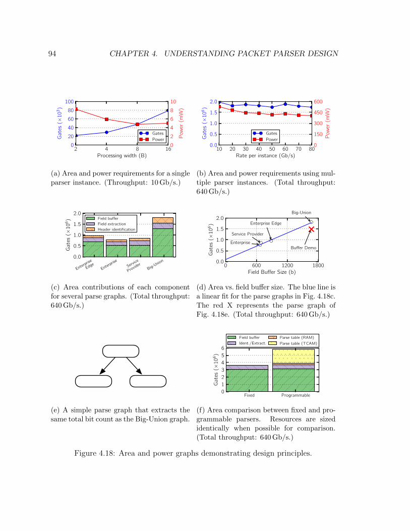
94 CHAPTER 4. UNDERSTANDING PACKET PARSER DESIGN
2 4 8 16Processing width (B)
0
20
40
60
80
100
Ga
tes
(×1
03)
Gates
Power
0
2
4
6
8
10
Po
wer
(mW
)
(a) Area and power requirements for a singleparser instance. (Throughput: 10 Gb/s.)
10 20 30 40 50 60 70 80Rate per instance (Gb/s)
0.0
0.5
1.0
1.5
2.0
Ga
tes
(×1
06)
Gates
Power
0
150
300
450
600
Po
wer
(mW
)
(b) Area and power requirements using mul-tiple parser instances. (Total throughput:640 Gb/s.)
Enterprise
EdgeEnterpris
e
Service
ProviderBig-U
nion0.0
0.5
1.0
1.5
2.0
Ga
tes
(×1
06) Field buffer
Field extraction
Header identification
(c) Area contributions of each componentfor several parse graphs. (Total throughput:640 Gb/s.)
0 600 1200 1800Field Buffer Size (b)
0.0
0.5
1.0
1.5
2.0
Ga
tes
(×1
06) Enterprise Edge
Enterprise
Service Provider
Big-Union
Buffer Demo
(d) Area vs. field buffer size. The blue line isa linear fit for the parse graphs in Fig. 4.18c.The red X represents the parse graph ofFig. 4.18e. (Total throughput: 640 Gb/s.)
(e) A simple parse graph that extracts thesame total bit count as the Big-Union graph.
Fixed Programmable0
1
2
3
4
5
6
Ga
tes
(×1
06)
Field buffer
Ident./Extract.
Parse table (RAM)
Parse table (TCAM)
(f) Area comparison between fixed and pro-grammable parsers. Resources are sizedidentically when possible for comparison.(Total throughput: 640 Gb/s.)
Figure 4.18: Area and power graphs demonstrating design principles.
4.5. DESIGN PRINCIPLES 95
The rate of a single parser instance does not scale indefinitely. Area and power
both increase (not shown) when approaching the maximum rate of a single instance.
Principle: Field buffers dominate area.
Figure 4.18c shows the parser area by functional block for several parse graphs. Field
buffers dominate the parser area, accounting for approximately two-thirds of the total
area.
There is little flexibility in the design of the field buffer: it must be built from
an array of registers to allow extracted fields to be sent in parallel to downstream
components (§4.3.1). This lack of flexibility implies that its size should be roughly
constant for a given parse graph, regardless of other design choices.
Principle: A parse graph’s extracted bit count determines the parser area
(for a fixed processing width).
Figure 4.18d plots total extracted bit count versus parser area for several parse graphs.
The straight line shows the linear best fit for the data points; all points lie very close
to this line.
Given that the field buffer dominates the area, one might expect that a parser’s
size can be determined predominantly by the total number of bits extracted. This
hypothesis is verified by the additional data point included on the plot for the simple
parse graph of Figure 4.18e. This graph consists of only three nodes, but those three
nodes extract the same number of bits as the big-union graph. The data point lies
just below that of the big-union graph—the small difference is accounted for by the
simple parse graph requiring simpler header identification and field extraction logic.
This principle follows from the previous principle: the number of extracted bits
determines the field buffer depth, and the field buffer dominates total parser area;
thus, the number of extracted bits should approximately determine the total parser
area.
96 CHAPTER 4. UNDERSTANDING PACKET PARSER DESIGN
4.5.3 Programmable parser design principles
The fixed parser design principles apply to programmable parser design, with the
additional principles outlined below.
Principle: The parser state table and field buffer area are the same order
of magnitude.
Figure 4.18f shows an area comparison between a fixed and a programmable parser.
The fixed design implements the big-union parse graph. Both parsers include 4 Kb
field buffers for comparison, and the programmable parser includes a 256 × 40 b
TCAM; lookups consist of an 8 b state value and 2 × 16 b header fields. This choice
of parameters yields a programmable design that is almost twice the area of the
fixed design, with the parser state table (TCAM and RAM) consuming roughly the
same area as the field buffer. Different TCAM sizes yield slightly different areas, but
exploration reveals that the TCAM area is on the same order of magnitude as the
field buffer when appropriately sized for a programmable parser.
It is important to note that designers size fixed parsers to accommodate only the
chosen parse graph, while they size programmable parsers to accommodate all ex-
pected parse graphs. Many resources are likely to remain unused when implementing
a simple parse graph using the programmable parser. For example, the enterprise
parse graph requires only 672 b of the 4 Kb field buffer.
The 4 Kb field buffer and the 256 × 40 b TCAM are more than sufficient to
implement all tested parse graphs. The TCAM and the field buffer are twice the size
required to implement the big-union parse graph.
Observation: Programmability costs 1.5− 3×.
Figure 4.18f shows one data point. However, comparisons across a range of parser
state table and field buffer sizes reveal that programmable parsers cost 1.5− 3× the
area of a fixed parser (for reasonable choices of table/buffer sizes).

4.5. DESIGN PRINCIPLES 97
TCAMInputs Entry count Width (b) Size (b)
1 113 24 2,7122 105 40 4,2003 99 56 5,5444 102 72 7,344
Table 4.1: Parse table entry count and TCAM size.
Observation: A programmable parser occupies 2% of die area.
Parsers occupy a small fraction of the switch chip. The fixed parser of Figure 4.18f
occupies 2.6 mm2, while the programmable parser occupies 4.4 mm2 in a 45 nm tech-
nology. A 64 × 10 Gb/s switch die is typically 200 – 400 mm2 today.1
Principle: Minimize the number of parse table lookup inputs.
Increasing the number of parse table lookup inputs allows the parser to identify more
headers per cycle, potentially decreasing the total number of table entries. However,
the cost of an additional lookup is paid by every entry in the table, regardless of the
number of lookups required by the entry.
Table 4.1 shows the required number of table entries and the total table size for
differing numbers of 16-bit lookup inputs with the big-union parse graph. A lookup
width of 16 bits is sufficient for most fields used to identify header types and lengths—
e.g., the Ethertype field is 16 bits. The parser uses a four byte input width and
contains a 16 byte internal buffer. The total number of table entries reduces slightly
when moving from one to three lookups, but the total size of the table increases
greatly because of the increased width. The designer should therefore minimize the
number of table inputs to reduce the total parser area because the parse state table
is one of the two main contributors to the area.
In this example, the number of parse table entries increases when the number of
lookups exceeds three. This is an artifact caused by the heuristic intended to reduce
the number of table entries. The heuristic considers each subgraph with multiple
1Source: private correspondence with switch chip vendors.

98 CHAPTER 4. UNDERSTANDING PACKET PARSER DESIGN
ingress edges in turn. The decision to remove a subgraph may impact the solution
of a later subgraph. In this instance, the sequence of choices made when performing
three lookups per cycle performs better than the choices made when performing four
lookups per cycle.
The exploration reveals that two 16 b lookup values provide a good balance be-
tween parse state table size and the ability to maintain line rate for a wide array of
header types. All common headers in use today are a minimum of four bytes, with
most also being a multiple of four bytes. Most four-byte headers contain only a single
lookup value, allowing two four-byte headers to be identified in a single cycle. Head-
ers shorter than four bytes are not expected in the future because little information
could be carried by such headers.
4.6 RMT switch parser
An RMT switch requires a programmable parser to enable definition of new headers.
The RMT switch of Chapter 3 contains a programmable parser design that closely
matches the one presented in §4.3.3.
Multiple parser instances provide the 640 Gb/s aggregate throughput. Each parser
operates at 40 Gb/s, requiring 16 parsers in total. Practical considerations, in con-
junction with the design principles of §4.5, led to my selection of the 40 Gb/s rate.
The switch’s I/O channels operate at 10 Gb/s, with the ability to gang four to-
gether to create a 40 Gb/s channel. Implementation is simplified when parsers operate
at integer fractions or multiples of 40 Gb/s, as channels can be statically allocated to
particular parser instances. Ideal candidate rates include 10, 20, 40, 80, and 160 Gb/s.
The design principles provide guidance as to which rate to select. Unfortunately
two principles are in tension, suggesting different choices. “Use fewer faster parsers
when aggregating parser instances” suggests selection of faster parsers, while “Min-
imize the number of parse table lookup inputs” suggests selection of slower parsers,
because faster parsers require more parse table lookup inputs to enable additional
headers to be parsed each cycle to meet the throughput requirement. I chose the
40 Gb/s rate as a balance between these two principles.
4.7. RELATED WORK 99
I chose the parser TCAM size to be 256 entries × 40 b; each entry matches the 8 b
parser state and two 16 b lookup values. Two lookup inputs are necessary to support
line rate parsing at 40 Gb/s across all tested parse graphs; a parser with a single
lookup input falls increasingly further behind when parsing long sequences of short
headers for certain parse graphs. The 256 entries are more than sufficient for all tested
parse graphs; the big-union graph occupied 105 entries when using two lookup inputs
(Table 4.1), leaving more than half the table available for more complex graphs.
4.7 Related work
Kangaroo [67] is a programmable parser that parses multiple headers per cycle. Kan-
garoo buffers all header data before parsing, which introduces latencies that are too
large for switches today. Attig [3] presents a language for describing header sequences,
together with an FPGA parser design and compiler. Kobiersky [66] also presents an
FPGA parser design and generator. Parsers are implemented in FPGAs not ASICs
in these works, leading to a different set of design choices. None of the works explore
design trade-offs or extract general parser design principles.
Much has been written about hardware-accelerated regular expression engines
(e.g., [80,109,110]) and application-layer parsers (e.g., [81,112]). Parsing is the explo-
ration of a small section of a packet directed by a parse graph, while regular expression
matching scans all bytes looking for regular expressions. Differences in the data re-
gions under consideration, the items to be found, and the performance requirements
lead to considerably different design decisions. Application-layer parsing frequently
involves regular expression matching.
Software parser performance can be improved via the use of a streamlined fast
path and a full slow path [68]. The fast path processes the majority of input data,
with the slow path activated only for infrequently seen input data. This technique
is not applicable to hardware parser design because switches must guarantee line
rate performance for worst-case traffic patterns; software parsers do not make such
guarantees.

100 CHAPTER 4. UNDERSTANDING PACKET PARSER DESIGN
Chapter 5
Application: Distributed hardware
While the majority of this thesis describes techniques to make the network more
flexible, the ultimate goal is to enable construction of a rich ecosystem of network
applications similar to that which exists in the world of computers. To that end, I
describe a novel application named OpenPipes that utilizes the flexible RMT switch
to construct complex packet processing systems. The application uses the network
to “plumb” arbitrary packet processing elements or modules together. OpenPipes is
agnostic to how modules are implemented, allowing software, hardware, and hybrid
systems to be built.
OpenPipes
OpenPipes allows researchers and developers to build systems that perform custom
processing on data streams flowing through a network. Example applications include
data compression, encryption, video transformation and encoding, and signal process-
ing. Systems are constructed by interconnecting processing modules. Key objectives
for the platform are:
Simplicity
Building systems that operate at line rate should be fast and easy.
Utilization of all resources
A designer should be able to use all resources at his or her disposal. The
101

102 CHAPTER 5. APPLICATION: DISTRIBUTED HARDWARE
platform should be agnostic to where modules are located when assembling
systems, allowing modules to reside in different physical devices. Moreover,
it should also be agnostic regarding how modules are implemented, allowing
modules to be implemented on CPUs, NPUs, FPGAs, and more.
Simplified module testing
Designers often prototype modules in software before implementing them in
hardware. The platform should leverage the effort invested in developing soft-
ware modules to aid in the verification of hardware modules.
Dynamic reconfiguration
It should be possible to modify a running system configuration without having
to halt for reconfiguration. This ability presents many possibilities, including
the following: scaling systems in response to demand, improving performance or
fixing bugs by replacing modules, and modifying system behavior by changing
the type and ordering of modules.
As is common in system design, the OpenPipes’ design assumes that systems are
partitioned into modules. OpenPipes plumbs modules together over the network,
re-plumbing them as the system is repartitioned and modules are moved. Designers
can move modules while the system is “live,” allowing for real-time experimentation
with different designs and partitions. The benefits of modularity for code re-use and
rapid prototyping are well-known [82,97].
An important aspect of OpenPipes is its agnosticism regarding how modules are
implemented. Designers may implement modules in any way, provided that each
module is network-connected and uses a standardized OpenPipes module interface.
A module can be a user-level process written in Java or C on a CPU, or it can be a
set of gates written in Verilog on an FPGA. A designer may implement a module in
software and test its behavior in the system before committing the design to hardware.
A designer can verify a module’s hardware implementation by including software and
hardware versions of the module in a live system; OpenPipes verifies correctness
by sending the same input to both versions and comparing their outputs to ensure
identical behavior.
103
The network
OpenPipes places several demands on the network. First, it needs a network in which
modules can move around easily and seamlessly under the control of the OpenPipes
platform. If each module has its own network address (e.g., an IP address), then ide-
ally, the module can move without having to change its address. Second, OpenPipes
needs the ability to bicast or multicast packets anywhere in the system—it may be
desirable to send the same packet to multiple versions of the same module for testing
or scaling or to multiple different modules for performing separate parallel compu-
tations. Finally, OpenPipes needs the ability to control the paths: it may wish to
select the lowest latency or highest bandwidth paths in order to provide performance
guarantees.
SDN is an ideal network technology, as it satisfies these requirements; compet-
ing network technologies aren’t suitable, as they fail one or more demands. With
SDN, the OpenPipes controller has full control over traffic flow within the network.
The controller can move modules and automatically adjust the paths between them
without changing module addresses; it can replicate packets anywhere within the
topology to send packets to multiple modules; and it can choose the queues to use in
each switch in order to guarantee bandwidth and/or latency between modules and,
hence, for the system as a whole.
As Chapters 2 and 3 have highlighted, there exists several match-action SDN
alternatives. Ideally, OpenPipes uses a custom packet format with a header tailored
to its signalling needs and which switches can match on and modify. This desire
to define and manipulate custom header formats makes the RMT model or, more
specifically, the RMT switch described in Chapter 3, ideal for use by OpenPipes.
Current OpenFlow switches do not allow a controller to define custom header formats;
however, as §5.3 shows, OpenFlow switches are sufficient to build a limited prototype
by shoehorning data into existing header fields.
At a high level, OpenPipes is just another way to create modular systems and
plumb them together using a standard module-to-module interface. The key difference
104 CHAPTER 5. APPLICATION: DISTRIBUTED HARDWARE
is that OpenPipes uses commodity networks to interconnect the modules. This allows
any device with a network connection to potentially host modules.
While chip design can usefully borrow ideas from networking to create intercon-
nected modules, it comes with difficulties. It is not clear what addressing scheme
to use for modules; modules could potentially use Ethernet MAC addresses, IP ad-
dresses, or something else. A common outcome is a combination of Ethernet and IP
addresses, plus a layer of encapsulation to create an overlay network between mod-
ules. Encapsulation provides a good way to pass traffic through firewalls and NAT
devices, but it always creates headaches when packets are made larger and need to
be fragmented. Encapsulation increases complexity in the network as more layers
and encapsulation formats are added; it seems to make the network more fragile and
less agile. A consequence of encapsulation is that it makes it harder for modules to
move around. If modules are to be re-allocated to another system, such as to another
hardware platform or to move to software for debugging and development, then the
address of each tunnel needs changing.
In a modular system that is split across the network—potentially at a great
distance—it is unclear how errors should be handled. Some modules will require
error control and retransmissions, whereas others might tolerate occasional packet
drops (e.g., the pipeline in a modular IPv4 router). Introducing an appropriate error-
handling mechanism into the module interface is a daunting task.
The remainder of this chapter describes OpenPipes in detail and addresses the chal-
lenges outlined above. It begins with an introduction to the high-level architecture.
Next, it discusses a number of implementation details, and finally, it presents an
example application that shows OpenPipes in action.
5.1 OpenPipes architecture
OpenPipes consists of three major components: a series of processing modules, a flex-
ible interconnect to plumb the modules together, and a controller that configures
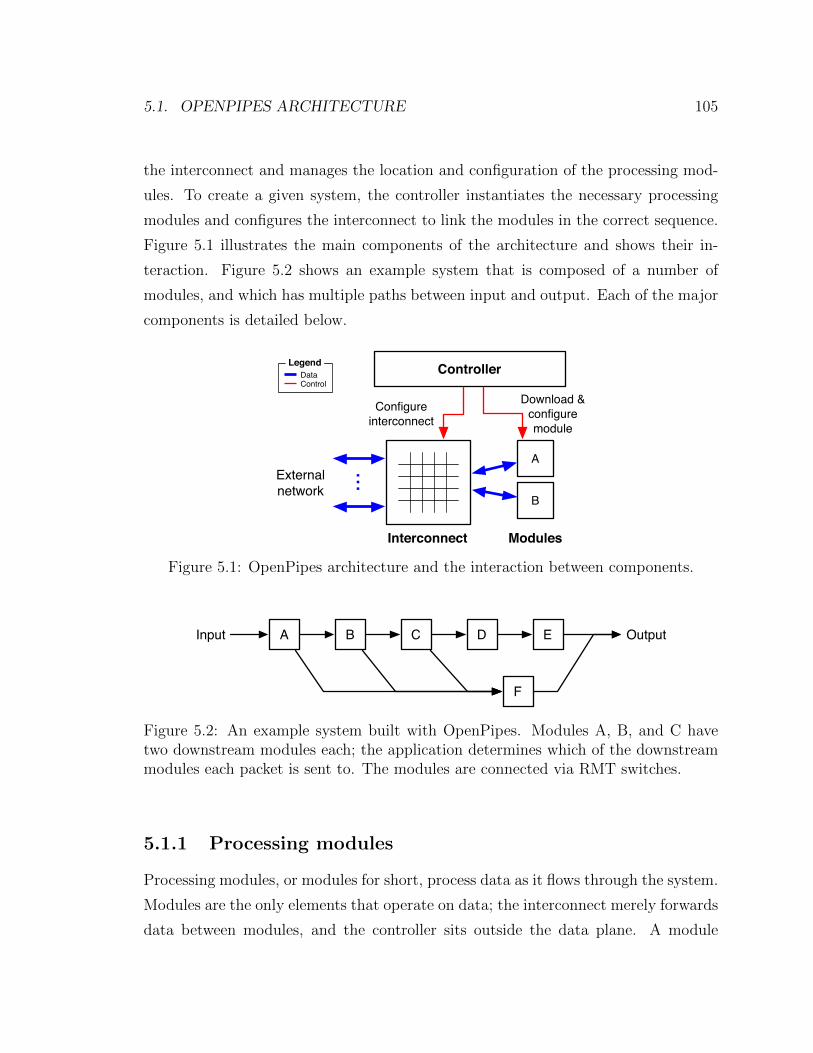
5.1. OPENPIPES ARCHITECTURE 105
the interconnect and manages the location and configuration of the processing mod-
ules. To create a given system, the controller instantiates the necessary processing
modules and configures the interconnect to link the modules in the correct sequence.
Figure 5.1 illustrates the main components of the architecture and shows their in-
teraction. Figure 5.2 shows an example system that is composed of a number of
modules, and which has multiple paths between input and output. Each of the major
components is detailed below.
A
B
Controller
Interconnect Modules
Externalnetwork
LegendDataControl
...
Configureinterconnect
Download &configuremodule
Figure 5.1: OpenPipes architecture and the interaction between components.
A B C D E
F
Input Output
Figure 5.2: An example system built with OpenPipes. Modules A, B, and C havetwo downstream modules each; the application determines which of the downstreammodules each packet is sent to. The modules are connected via RMT switches.
5.1.1 Processing modules
Processing modules, or modules for short, process data as it flows through the system.
Modules are the only elements that operate on data; the interconnect merely forwards
data between modules, and the controller sits outside the data plane. A module
106 CHAPTER 5. APPLICATION: DISTRIBUTED HARDWARE
designer is free to implement any processing that he or she wishes inside a module;
he or she can choose to implement a single function or multiple functions and choose
to implement simple or complex functions. In general, modules are likely to perform
a single, well-defined function, as it is well-known that this tends to maximize reuse
in other systems [82,97].
OpenPipes places two requirements on modules: they must connect to the net-
work, and they must use a standardized packet format. The interconnect makes
routing decisions using fields within the packet headers; §5.1.2 discusses the intercon-
nect and the packet format. Beyond these requirement, modules may perform any
processing that the designer chooses. Modules may transform packets as they flow
through the system, outputting one or more packets in response to each input packet;
drop packets; and asynchronously output packets independent of packet reception,
allowing tasks such as the transmission of periodic probe packets.
In general, designers should build modules to operate with zero knowledge of the
system. OpenPipes does not inform modules of their locations or their neighbors.
Modules should process all data sent to them, and they should not make assumptions
about the processing that upstream neighbors have performed or that downstream
neighbors will perform. The user is responsible for ensuring that the data input to a
module conforms to the type and format expected by the module; in a more sophis-
ticated scheme, modules would inform the controller of their input and output, and
the controller would enforce connection between compatible modules only. Designing
modules to operate independently of other modules aids reuse by allowing modules
to be placed anywhere within a system, in any order, as determined by the controller
and system operator.
Although modules should operate with zero knowledge of the system, designers
may build modules that share and use metadata about packets. One module can tag
a packet with metadata, and a subsequent module can base processing decisions on
that metadata. For example, a meter module may measure the data rate of a video
stream and tag each packet with a “color” that indicates whether the video rate
exceeds some threshold. A shaper module located downstream can then re-encode
the video at a lower bit-rate when the color indicates that the threshold was exceeded.
5.1. OPENPIPES ARCHITECTURE 107
The advantage of this approach is that other modules can use the same metadata; for
example, a policer module can use the color to drop traffic exceeding the threshold.
§5.1.2 documents the metadata communication mechanism in the description of the
packet format.
Module ports
A module may have any number of ports its designer chooses. Many devices used to
host modules have only one physical port, restricting the module to a single port that
is used for both input and output. Although a module may have only one physical
port, it can provide multiple logical ports. The OpenPipes routing header (§5.1.2)
contains a field that indicates the logical port; a module reads this field on packet
ingress to identify the incoming logical port, and it sets this field on packet egress to
indicate the logical output port that it is using.
Modules may use different output ports, either physical or logical, to indicate
attributes of the data. For example, a checksum validation module can use different
output ports to indicate whether a packet contains a valid or an invalid checksum.
The OpenPipes controller can instruct the interconnect to route different outputs to
different destinations. The controller could route the output port corresponding to
packets with valid checksums to a “normal” processing pipeline, and it could route
invalid traffic to an error-handling pipeline. Referring to Figure 5.2, modules A, B,
and C each have two outputs; one output from module A is connected to module B
and the other to module F .
Configurable parameters
Many modules provide configurable parameters that impact processing. For example,
the meter module described above should provide a threshold parameter to allow con-
figuration of the threshold rate. Parameters are read and modified by the controller.
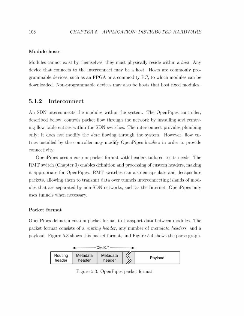
108 CHAPTER 5. APPLICATION: DISTRIBUTED HARDWARE
Module hosts
Modules cannot exist by themselves; they must physically reside within a host. Any
device that connects to the interconnect may be a host. Hosts are commonly pro-
grammable devices, such as an FPGA or a commodity PC, to which modules can be
downloaded. Non-programmable devices may also be hosts that host fixed modules.
5.1.2 Interconnect
An SDN interconnects the modules within the system. The OpenPipes controller,
described below, controls packet flow through the network by installing and remov-
ing flow table entries within the SDN switches. The interconnect provides plumbing
only; it does not modify the data flowing through the system. However, flow en-
tries installed by the controller may modify OpenPipes headers in order to provide
connectivity.
OpenPipes uses a custom packet format with headers tailored to its needs. The
RMT switch (Chapter 3) enables definition and processing of custom headers, making
it appropriate for OpenPipes. RMT switches can also encapsulate and decapsulate
packets, allowing them to transmit data over tunnels interconnecting islands of mod-
ules that are separated by non-SDN networks, such as the Internet. OpenPipes only
uses tunnels when necessary.
Packet format
OpenPipes defines a custom packet format to transport data between modules. The
packet format consists of a routing header, any number of metadata headers, and a
payload. Figure 5.3 shows this packet format, and Figure 5.4 shows the parse graph.
Routing header
Metadata header PayloadMetadata
header
Qty: [0,*]
Figure 5.3: OpenPipes packet format.

5.1. OPENPIPES ARCHITECTURE 109
Comparison(Metadata)
Routing
Figure 5.4: OpenPipes parse graph. The interconnect only processes the comparisonmetadata header; all other metadata headers are ignored.
The routing header (Figure 5.5a) contains two fields: a port/stream identifier and
a count of the number of metadata headers that follow. As the name implies, the
routing header is the primary header that OpenPipes uses to route traffic within
the interconnect. A module transmitting a packet writes a value in the port/stream
field to indicate the packet’s logical output port (§5.1.1). The switches rewrite the
port/stream field at each hop to allow identification of flows or streams that share a
link.
Port / stream Metadata hdr. count
3 B 1 B
(a) Routing header.
Type Value
7 B1 B
(b) Metadata header.
Figure 5.5: OpenPipes header formats.
Metadata headers (Figure 5.5b) communicate information about the payload or
some state within the modules that processed a packet. The header consists of two
fields: a type and a value. The type indicates what the metadata is, which, in turn,
determines the meaning and format of the value field. The metadata header concept
is borrowed from the NetFPGA [72] processing pipeline, in which the headers com-
municate information about each packet between modules; for example, one standard
header conveys a packet’s length, source port, and destination port(s).
110 CHAPTER 5. APPLICATION: DISTRIBUTED HARDWARE
Metadata types may be either system-defined or module-defined. A “1” in the
type field’s MSB indicates system-defined, and a “0” indicates module-defined. Open-
Pipes currently defines only one system type: a comparison identifier (0x81). The
comparison identifier indicates the module source and a sequence number for use by
the comparison module; §5.2.1 provides more detail. To simplify parsing, system-
defined metadata must appear before module-defined metadata.
Modules use module-defined metadata to indicate data that the system doesn’t
provide about each packet. The example presented earlier involved a meter and a
shaper. The meter measures video data rate and tags packets with a color to indicate
when the rate exceeds a threshold; the shaper re-encodes video at a lower rate when
the color indicates that the threshold was exceeded. The color is communicated in
a metadata header. Two modules wishing to communicate data must agree on the
metadata’s format and type number; it is suggested that the controller assign type
numbers dynamically.
Any module may add, modify, or delete any number of metadata headers from
packets flowing through the system. Designers should pass unknown metadata head-
ers from input to output transparently, thereby allowing communication between
modules regardless of what modules sit between them.
Addressing, routing, and path determination
A user builds systems in OpenPipes by composing modules. Modules process data,
and the interconnect transports data between them. OpenPipes does not inform
modules of their neighbors, making it is impossible for modules to address their
output to modules immediately downstream.
The controller is the only component within the system that knows the desired
ordering of modules. The controller routes traffic between modules in the interconnect
by installing appropriate flow entries in the switches. The flow entries for a connection
between modules establishes a path from the output of one module to the input of
the next.
Referring to Figure 5.2, module A connects to modules B and F . The controller
installs two sets of rules in this example: one to route traffic from A to B and one to
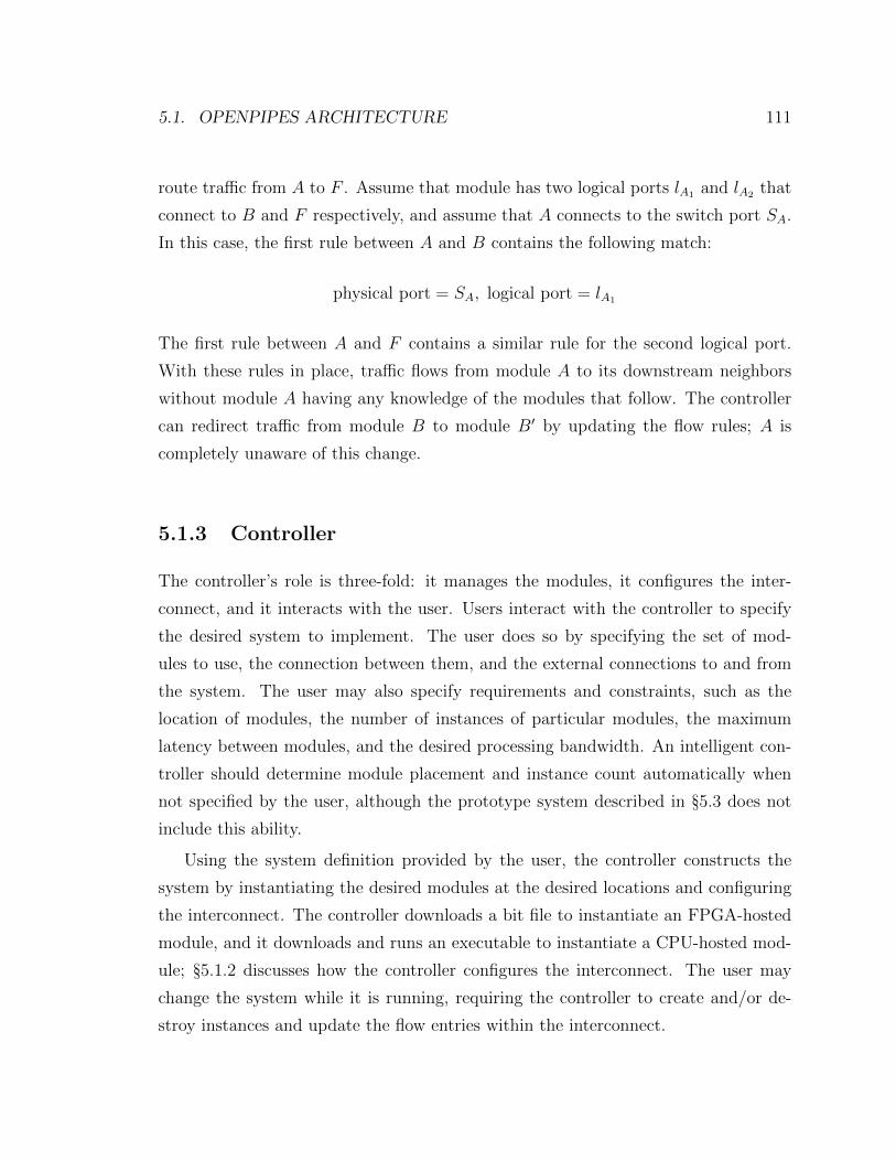
5.1. OPENPIPES ARCHITECTURE 111
route traffic from A to F . Assume that module has two logical ports lA1 and lA2 that
connect to B and F respectively, and assume that A connects to the switch port SA.
In this case, the first rule between A and B contains the following match:
physical port = SA, logical port = lA1
The first rule between A and F contains a similar rule for the second logical port.
With these rules in place, traffic flows from module A to its downstream neighbors
without module A having any knowledge of the modules that follow. The controller
can redirect traffic from module B to module B′ by updating the flow rules; A is
completely unaware of this change.
5.1.3 Controller
The controller’s role is three-fold: it manages the modules, it configures the inter-
connect, and it interacts with the user. Users interact with the controller to specify
the desired system to implement. The user does so by specifying the set of mod-
ules to use, the connection between them, and the external connections to and from
the system. The user may also specify requirements and constraints, such as the
location of modules, the number of instances of particular modules, the maximum
latency between modules, and the desired processing bandwidth. An intelligent con-
troller should determine module placement and instance count automatically when
not specified by the user, although the prototype system described in §5.3 does not
include this ability.
Using the system definition provided by the user, the controller constructs the
system by instantiating the desired modules at the desired locations and configuring
the interconnect. The controller downloads a bit file to instantiate an FPGA-hosted
module, and it downloads and runs an executable to instantiate a CPU-hosted mod-
ule; §5.1.2 discusses how the controller configures the interconnect. The user may
change the system while it is running, requiring the controller to create and/or de-
stroy instances and update the flow entries within the interconnect.
112 CHAPTER 5. APPLICATION: DISTRIBUTED HARDWARE
As described earlier, some modules provide configurable parameters. Users specify
module parameter values to the controller, and the controller programs the values
into the appropriate modules. The controller must take care when moving modules
because it must also move the configurable parameters. Moving a module typically
involves instantiating a new copy of the module at the new location and destroying
the old instance, hence the need to move the parameters. A module should expose
all state that requires moving as configurable parameters.
5.2 Plumbing the depths
The previous section introduced the OpenPipes architecture and described its major
components. This section attempts to expand understanding by delving into several
operational details, including testing, flow and error control, and platform limitations.
5.2.1 Testing via output comparison
OpenPipes aids in module testing by enabling the in-situ comparison of multiple
versions of a module in a running system. The testing process sends the same input
data to two versions of the module under test and compares the two modules’ output.
Non-identical streams indicate that one of the modules is functioning incorrectly.
The rationale behind this approach is that a functionally correct software proto-
type provides a behavioral model against which to verify hardware. Designers are
likely to build software prototypes before implementing hardware in many situations,
because software prototypes allow designers to quickly verify ideas. By using the soft-
ware prototype as a behavioral model for verification, the designer gains additional
benefit from the effort invested in building the prototype.
In-situ testing allows testing with large volumes of real data. Simulated data
sets often fail to capture all data characteristics that reveal bugs, and hardware sim-
ulations execute orders of magnitude more slowly than the modules that they are
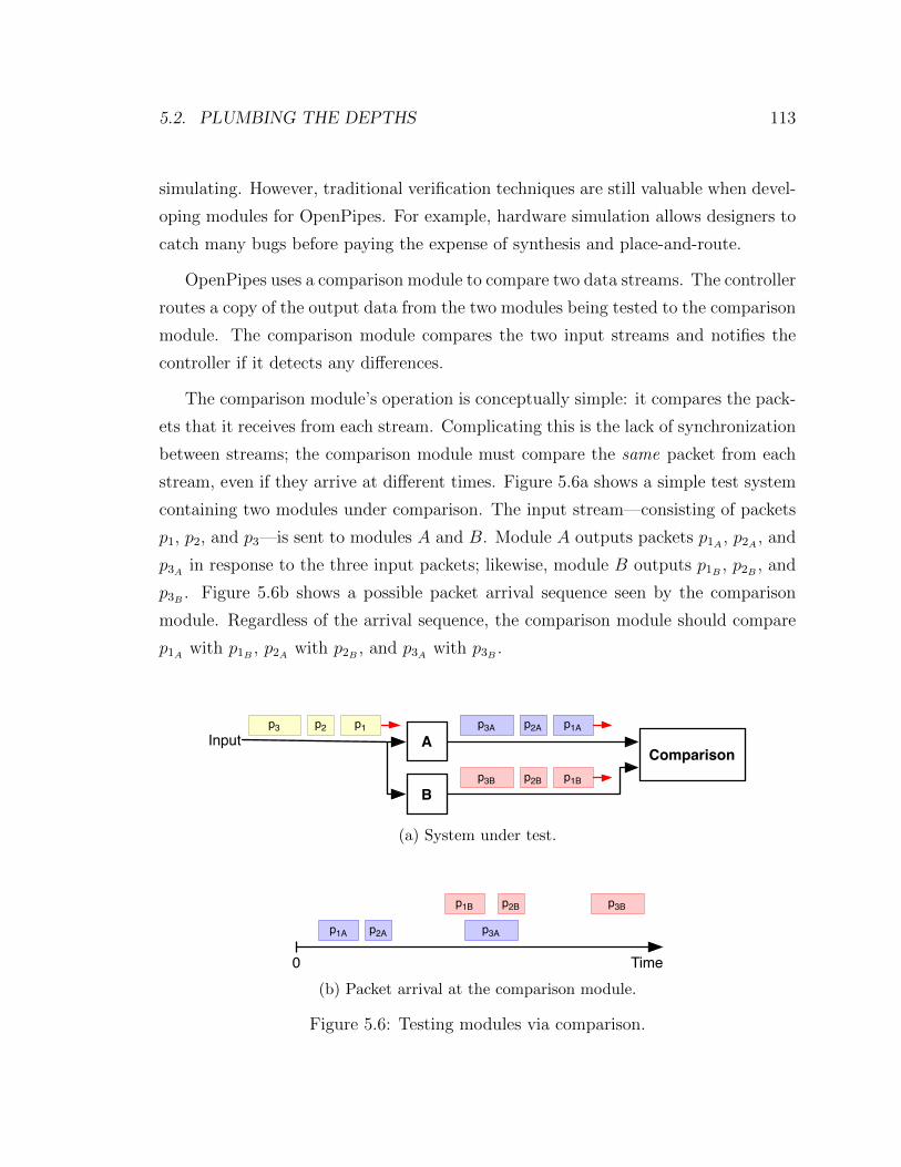
5.2. PLUMBING THE DEPTHS 113
simulating. However, traditional verification techniques are still valuable when devel-
oping modules for OpenPipes. For example, hardware simulation allows designers to
catch many bugs before paying the expense of synthesis and place-and-route.
OpenPipes uses a comparison module to compare two data streams. The controller
routes a copy of the output data from the two modules being tested to the comparison
module. The comparison module compares the two input streams and notifies the
controller if it detects any differences.
The comparison module’s operation is conceptually simple: it compares the pack-
ets that it receives from each stream. Complicating this is the lack of synchronization
between streams; the comparison module must compare the same packet from each
stream, even if they arrive at different times. Figure 5.6a shows a simple test system
containing two modules under comparison. The input stream—consisting of packets
p1, p2, and p3—is sent to modules A and B. Module A outputs packets p1A , p2A , and
p3A in response to the three input packets; likewise, module B outputs p1B , p2B , and
p3B . Figure 5.6b shows a possible packet arrival sequence seen by the comparison
module. Regardless of the arrival sequence, the comparison module should compare
p1A with p1B , p2A with p2B , and p3A with p3B .
A
B
Comparison
p1p2p3 p1Ap2Ap3A
p1Bp2Bp3B
Input
(a) System under test.
Time0
p1A p2A p3A
p1B p2B p3B
(b) Packet arrival at the comparison module.
Figure 5.6: Testing modules via comparison.
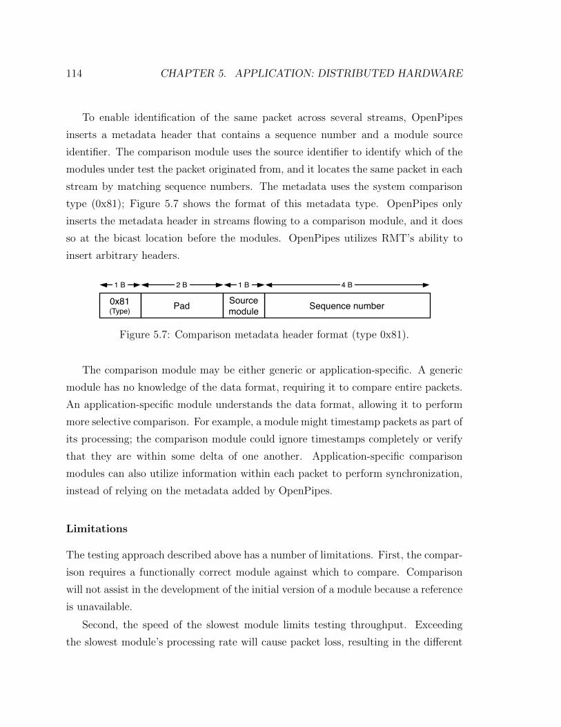
114 CHAPTER 5. APPLICATION: DISTRIBUTED HARDWARE
To enable identification of the same packet across several streams, OpenPipes
inserts a metadata header that contains a sequence number and a module source
identifier. The comparison module uses the source identifier to identify which of the
modules under test the packet originated from, and it locates the same packet in each
stream by matching sequence numbers. The metadata uses the system comparison
type (0x81); Figure 5.7 shows the format of this metadata type. OpenPipes only
inserts the metadata header in streams flowing to a comparison module, and it does
so at the bicast location before the modules. OpenPipes utilizes RMT’s ability to
insert arbitrary headers.
0x81(Type) Pad Sequence numberSource
module
4 B1 B 2 B 1 B
Figure 5.7: Comparison metadata header format (type 0x81).
The comparison module may be either generic or application-specific. A generic
module has no knowledge of the data format, requiring it to compare entire packets.
An application-specific module understands the data format, allowing it to perform
more selective comparison. For example, a module might timestamp packets as part of
its processing; the comparison module could ignore timestamps completely or verify
that they are within some delta of one another. Application-specific comparison
modules can also utilize information within each packet to perform synchronization,
instead of relying on the metadata added by OpenPipes.
Limitations
The testing approach described above has a number of limitations. First, the compar-
ison requires a functionally correct module against which to compare. Comparison
will not assist in the development of the initial version of a module because a reference
is unavailable.
Second, the speed of the slowest module limits testing throughput. Exceeding
the slowest module’s processing rate will cause packet loss, resulting in the different
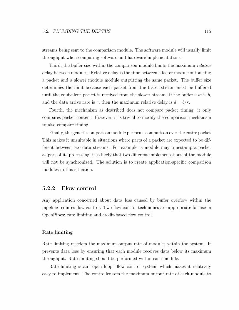
5.2. PLUMBING THE DEPTHS 115
streams being sent to the comparison module. The software module will usually limit
throughput when comparing software and hardware implementations.
Third, the buffer size within the comparison module limits the maximum relative
delay between modules. Relative delay is the time between a faster module outputting
a packet and a slower module module outputting the same packet. The buffer size
determines the limit because each packet from the faster stream must be buffered
until the equivalent packet is received from the slower stream. If the buffer size is b,
and the data arrive rate is r, then the maximum relative delay is d = b/r.
Fourth, the mechanism as described does not compare packet timing; it only
compares packet content. However, it is trivial to modify the comparison mechanism
to also compare timing.
Finally, the generic comparison module performs comparison over the entire packet.
This makes it unsuitable in situations where parts of a packet are expected to be dif-
ferent between two data streams. For example, a module may timestamp a packet
as part of its processing; it is likely that two different implementations of the module
will not be synchronized. The solution is to create application-specific comparison
modules in this situation.
5.2.2 Flow control
Any application concerned about data loss caused by buffer overflow within the
pipeline requires flow control. Two flow control techniques are appropriate for use in
OpenPipes: rate limiting and credit-based flow control.
Rate limiting
Rate limiting restricts the maximum output rate of modules within the system. It
prevents data loss by ensuring that each module receives data below its maximum
throughput. Rate limiting should be performed within each module.
Rate limiting is an “open loop” flow control system, which makes it relatively
easy to implement. The controller sets the maximum output rate of each module to
116 CHAPTER 5. APPLICATION: DISTRIBUTED HARDWARE
ensure that congestion never occurs within the system. Because congestion can never
occur, modules never need to notify each other or the controller of congestion.
This mechanism is most suitable when modules process data at near-constant
rates. This allows the controller to send data to a module at a chosen rate, knowing
that the module will always be able to process data at that rate. The mechanism
performs poorly in situations where a module’s throughput varies considerably; in
such situations, the controller must limit data sent to the module to the module’s
minimum sustained throughput.
To use this mechanism, modules must provide the ability to set their maximum
output rate. The module interface in a standard module template can include generic
rate limiting logic. Modules must report two pieces of data to the controller: their
maximum input rate and the relationship between input and output rate.
The controller sets rates throughout the system. It calculates rates using the
throughputs and ratios reported by modules, together with link capacities within the
interconnect. Rate calculations must consider ripple-on effects where the rate limit of
one module restricts the rate of every preceding module. For example, assume that
modules A, B, and C are connected in series (Figure 5.8), and assume their maximum
throughputs are tA, tB, and tC respectively. Module B’s output rate should be set
to rB = tC , and module A’s output rate should be set to rA = max(tB, rB) =
max(tB, rB).
Max inputrate = X
Max outputrate = X
A B C
➁➀➂
Figure 5.8: Rate limit information must “propagate” backward through the system.Module C has a maximum input rate of X, therefore the maximum output rates ofmodules A and B should be limited to X. Buffer overflow would occur in B if A’s ratewas not limited to X. (Note: this assumes that the output rate of B is identical toit’s input rate.)
5.2. PLUMBING THE DEPTHS 117
More correctly, each module should report a maximum input rate and an input-
to-output relationship. Assume A’s maximum input rate is IA and its input-to-
output relationship is ioA; assume similarly for B and C. In this case, the controller
should set module B’s output rate to rB = IC , and module A’s output rate to rA =
max(IB, rB/ioB) = max(IB, IC/ioB).
Credit-based flow control
Credit-based flow control [69] is a mechanism in which data flow is controlled via
the distribution of transmission credits. A downstream element issues credits to
an upstream element. An upstream element may transmit as much data as it has
credits for; once it exhausts its credits, it must pause until the downstream element
grants more credits. Credit-based flow control is most beneficial when a module’s
throughput varies considerably because it allows the module to adjust its receiving
rate to match its current throughput. Rate limiting in such situations would limit
the module’s input to the lowest sustained throughput, thereby failing to capitalize
when the module is capable of processing data at a higher rate.
Credit-based flow control is a “closed loop” flow control system. It is more complex
to implement than rate limiting because the adjacent module must coordinate to allow
data transmission. Contrast this with rate limiting, in which a module may transmit
data continuously at its permitted rate without regard to the state of other modules.
Credit-based flow control requires input buffering to accommodate transmission
delays between modules. An upstream module that exhausts its credits must wait
for credits from the downstream module before transmitting more data. If modules
A and B are connected in sequence, it takes a minimum of one round-trip time for B
to issue a credit to A and receive the resulting packet from A. To prevent a module
from sitting idle due to an empty buffer, the input buffer depth D must be at least
D = RTT × BW , where BW is the bandwidth of a link and RTT is the round-trip
time. This equates to 125 KB for a link with BW = 1 Gb/s and RTT = 1 ms.
118 CHAPTER 5. APPLICATION: DISTRIBUTED HARDWARE
Challenge: one-to-many and many-to-one connections
Flow control is complicated by connections between modules that are not one-to-one.
One-to-many connections, in which one upstream module connects directly to mul-
tiple downstream modules, require that the upstream module respect the processing
limits of all downstream modules. Many-to-one connections, in which multiple up-
stream modules directly connect to a single downstream module, require that the
aggregate data from all upstream modules is less than the processing limit of the
downstream module.
One-to-many connections are simple when using rate limiting: the controller limits
the upstream module to the input rate of the slowest downstream module. One-
to-many connections complicate credit-based flow control because each downstream
module may issue different numbers of credits. The solution is for the upstream
module to individually track the credits issued by each downstream module and to
transmit only when credits are available from all modules. This change increases the
amount of state that the upstream module must track, and it increases the complexity
of the transmit/pause logic.
OpenPipes handles many-to-one connections by splitting the rate or credits be-
tween the upstream modules. Although this prevents overload of the downstream
module, it often leads to underutilization. OpenPipes is unable to give an unused al-
lotment of rate or credits from one module to another module. The credit mechanism
must be modified slightly to force modules to return unused credits after a period of
time to prevent a single idle module from accumulating all of the credits.
5.2.3 Error control
Many applications will require inter-module error control to prevent data loss or
corruption. Not all applications require such mechanisms; some may be tolerant of
errors, while others may use an end-to-end error control mechanism. Several error
control mechanisms are available to meet differing application needs: error detection,
correction, and recovery.

5.2. PLUMBING THE DEPTHS 119
Error detection utilizes checksums [115], hashes [116], or similar integrity veri-
fication mechanisms. An application may use error detection to prevent erroneous
data from propagating through the processing pipeline or as part of an error recovery
mechanism (see below). An application’s response to detected errors when not using
a recovery mechanism is application-specific and is not discussed further.
Error correction utilizes mechanisms that introduce redundancy in the data, such
as error-correcting codes [71]. Error correction mechanisms repair minor errors in the
data stream without requiring retransmission.
Error recovery utilizes a combination of error detection and retransmission [35].
The sender retransmits packets that are erroneously received or lost, requiring the
sender to buffer copies of all sent data. The sender flushes data from its buffer when
it receives acknowledgement of correct reception.
5.2.4 Multiple modules per host
The discussion thus far has implied that hosts only host a single module at any
instant. A single host can trivially host a single module, but a single host can also
host multiple modules simultaneously. OpenPipes requires the ability to route traffic
to each module within a host, leading to two alternate approaches: the host may
provide a switch internally to route data to the appropriate module, or the host
provides separate physical interfaces for each module.
Providing a switch inside the host allows the use of a single physical connection
between the host and the interconnect. The internal switch sits between the external
interconnect and each of the modules, effectively extending the interconnect inside
the host. The internal switch must provide an SDN interface to allow configuration
by the controller.
Providing a separate physical interface for each module allows all host resources to
be dedicated to modules; the internal switch approach requires some host resources to
be dedicated to the internal switch. In this scenario, the number of physical interfaces
limits the number of modules.
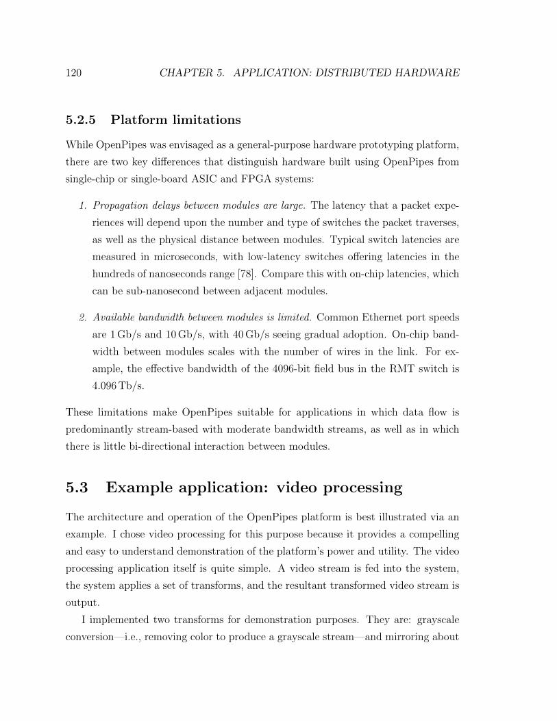
120 CHAPTER 5. APPLICATION: DISTRIBUTED HARDWARE
5.2.5 Platform limitations
While OpenPipes was envisaged as a general-purpose hardware prototyping platform,
there are two key differences that distinguish hardware built using OpenPipes from
single-chip or single-board ASIC and FPGA systems:
1. Propagation delays between modules are large. The latency that a packet expe-
riences will depend upon the number and type of switches the packet traverses,
as well as the physical distance between modules. Typical switch latencies are
measured in microseconds, with low-latency switches offering latencies in the
hundreds of nanoseconds range [78]. Compare this with on-chip latencies, which
can be sub-nanosecond between adjacent modules.
2. Available bandwidth between modules is limited. Common Ethernet port speeds
are 1 Gb/s and 10 Gb/s, with 40 Gb/s seeing gradual adoption. On-chip band-
width between modules scales with the number of wires in the link. For ex-
ample, the effective bandwidth of the 4096-bit field bus in the RMT switch is
4.096 Tb/s.
These limitations make OpenPipes suitable for applications in which data flow is
predominantly stream-based with moderate bandwidth streams, as well as in which
there is little bi-directional interaction between modules.
5.3 Example application: video processing
The architecture and operation of the OpenPipes platform is best illustrated via an
example. I chose video processing for this purpose because it provides a compelling
and easy to understand demonstration of the platform’s power and utility. The video
processing application itself is quite simple. A video stream is fed into the system,
the system applies a set of transforms, and the resultant transformed video stream is
output.
I implemented two transforms for demonstration purposes. They are: grayscale
conversion—i.e., removing color to produce a grayscale stream—and mirroring about
5.3. EXAMPLE APPLICATION: VIDEO PROCESSING 121
an axis. A separate module provides each transform. An operator of the system can
apply multiple transforms to a video stream by connecting the transform modules
in series. In addition to the transforms, I implemented a module that identifies the
predominant color within a video stream. This module provides one output for each
recognized predominant color. An operator can connect each output to a different set
of downstream modules, allowing different sets of transforms to be applied to different
colored videos. Finally, I implemented a comparison module that compares two video
streams. This module aids testing and development by module implementation to be
tested against a known-good implementation.
The operator can customize video processing by connecting and configuring the
modules within the system. For example, the operator can convert all video to
grayscale by instantiating the grayscale module and sending all video to the module.
Alternatively, the operator can vertically mirror red-colored videos while converting
all other videos to grayscale; they do so by sending all video to the color identification
module, connecting the identification module’s red output to the mirroring module,
and connecting all other outputs to the grayscale module.
Figure 5.9 depicts the video processing application graphically. The diagram shows
the input and output streams, a set of transforms, the color identification module,
and an example system configuration. Figure 5.12 shows a screenshot of the system
in action.
Video Processing System
Predominant Color
Identification
Grayscale Conversion
Video Inversion
Figure 5.9: Video processing application transforms video as it flows through thesystem. The OpenPipes application is the region inside the dotted rectangle.
122 CHAPTER 5. APPLICATION: DISTRIBUTED HARDWARE
RMT switches were unavailable at the time of writing. As a result, the demon-
stration system uses regular OpenFlow switches to provide the interconnect. This
prevented the use of custom headers, requiring the repurposing of existing headers.
5.3.1 Implementation
The major components of the demonstration system are the controller, the intercon-
nect, the modules, the module hosts, and a graphical user interface (GUI) to facilitate
interaction with the operator. Implementation details of each of these components
are provided below.
Controller
The OpenPipes controller is implemented in Python atop the NOX [42] OpenFlow
control platform. The OpenPipes controller consists of approximately 1,800 lines of
executable code, with additional lines for commenting and whitespace. I designed
the controller to be application-independent—i.e., the controller should be suitable
for use in applications other than video processing.
The controller functionality falls into several broad categories. They are as fol-
lows: GUI communication, module host communication, interconnect configuration,
and topology tracking. The GUI communication functionality allows the GUI and
the controller to interact. The controller maintains databases of the following: the
current network topology, including the active module hosts; the known modules; and
the current set of active modules and their interconnection. The controller communi-
cates this information to the GUI, which displays this information graphically to the
operator; the operator can then use the GUI to reconfigure the system.
A simple text-based socket is used for communication between the controller
and the GUI. The GUI sends simple commands to the controller to modify the
system configuration, such as instantiate-module, delete-module, connect, and
disconnect. The controller performs the appropriate system modifications in re-
sponse to commands from the GUI. The controller may also send messages to the
GUI to notify it of system changes, such as host-added and link-added.
5.3. EXAMPLE APPLICATION: VIDEO PROCESSING 123
Module host communication functionality allows module hosts to interact with
the controller. The controller instructs module hosts to download particular modules
and to configure parameters within each module, and the module hosts notify the
controller of changes to the module state. A simple text-based socket is used for this
communication, similar to the GUI-controller communication.
Interconnect configuration functionality translates the desired system configura-
tion into the appropriate set of flow rules for each switch. To translate a single
connection between two modules, the controller must: i) identify the location of the
two modules in the system; ii) calculate a route between the modules; and iii) install
flow table entries for each link on the chosen route. The first flow rule in the first
switch must match only the traffic corresponding to the selected logical output port.
The logical port field is rewritten on a hop-by-hop basis to distinguish between flows
sharing the link.
The topology tracking functionality monitors the state of the topology and trig-
gers rerouting of flows when necessary. For example, flows must be rerouted when
a link carrying them goes down. Topology tracking utilizes the topology learning
functionality provided by NOX.
Interconnect
The interconnect consists of multiple OpenFlow switches connected in a non-structured
topology (Figure 5.10). The demonstration system uses OpenFlow switches because
RMT switches were unavailable at the time of writing.
The topology consists mostly of switches and hosts located at Stanford University,
although it includes one remote switch and one remote host. The Internet2 [58] PoP
in Los Angeles hosts the remote switch, which is connected via a MAC-in-IP tunnel
that encapsulates entire packets. The OpenPipes controller is unaware of the tunnel
to the remote switch and sees a direct connection between the local network and
the remote switch. The topology’s ad-hoc structure arose from the physical location
of switches within the network and the links between them. The topology clearly
demonstrates OpenPipes’ ability to build systems from geographically distributed
hardware.
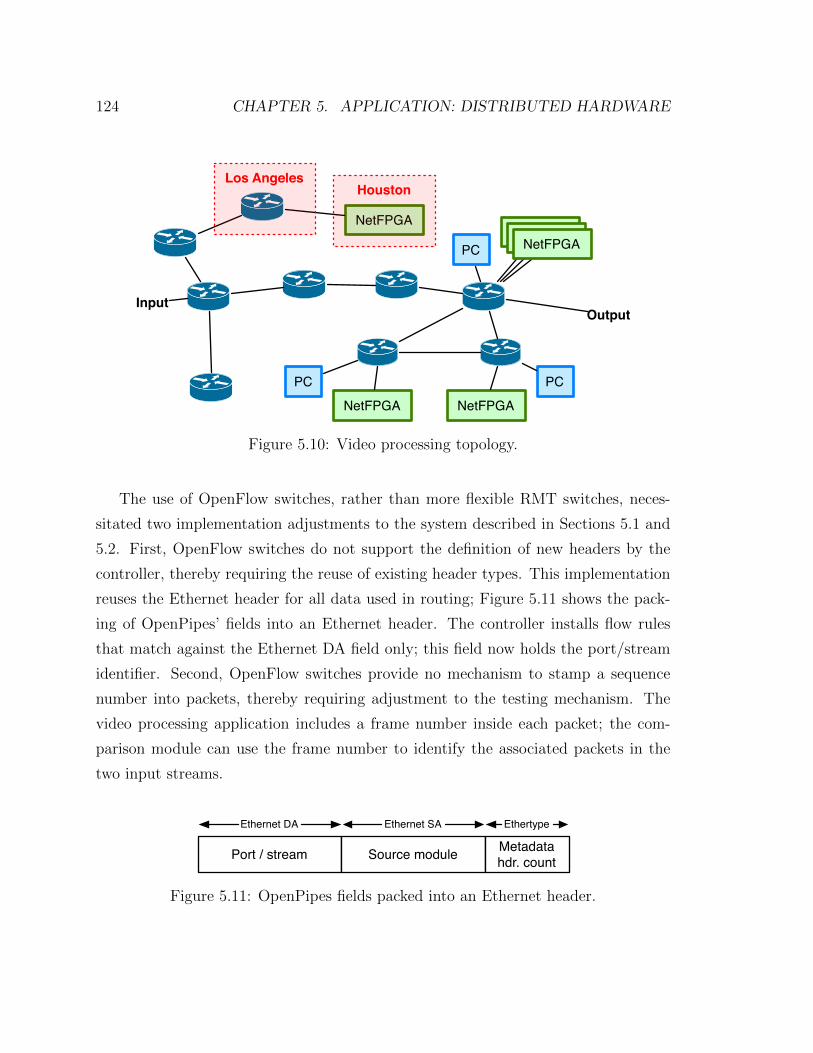
124 CHAPTER 5. APPLICATION: DISTRIBUTED HARDWARE
InputOutput
NetFPGANetFPGA
NetFPGA
PC PC
PCNetFPGANetFPGANetFPGA
Los AngelesHouston
Figure 5.10: Video processing topology.
The use of OpenFlow switches, rather than more flexible RMT switches, neces-
sitated two implementation adjustments to the system described in Sections 5.1 and
5.2. First, OpenFlow switches do not support the definition of new headers by the
controller, thereby requiring the reuse of existing header types. This implementation
reuses the Ethernet header for all data used in routing; Figure 5.11 shows the pack-
ing of OpenPipes’ fields into an Ethernet header. The controller installs flow rules
that match against the Ethernet DA field only; this field now holds the port/stream
identifier. Second, OpenFlow switches provide no mechanism to stamp a sequence
number into packets, thereby requiring adjustment to the testing mechanism. The
video processing application includes a frame number inside each packet; the com-
parison module can use the frame number to identify the associated packets in the
two input streams.
Port / stream Source module Metadatahdr. count
Ethernet DA Ethernet SA Ethertype
Figure 5.11: OpenPipes fields packed into an Ethernet header.
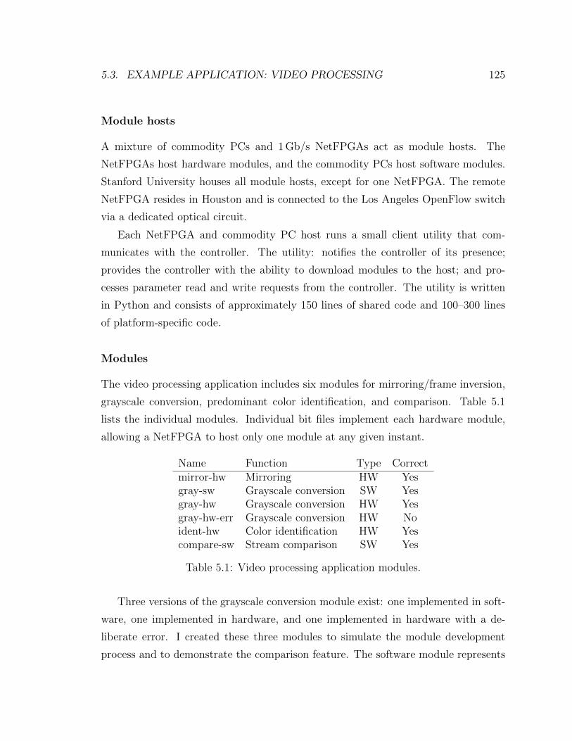
5.3. EXAMPLE APPLICATION: VIDEO PROCESSING 125
Module hosts
A mixture of commodity PCs and 1 Gb/s NetFPGAs act as module hosts. The
NetFPGAs host hardware modules, and the commodity PCs host software modules.
Stanford University houses all module hosts, except for one NetFPGA. The remote
NetFPGA resides in Houston and is connected to the Los Angeles OpenFlow switch
via a dedicated optical circuit.
Each NetFPGA and commodity PC host runs a small client utility that com-
municates with the controller. The utility: notifies the controller of its presence;
provides the controller with the ability to download modules to the host; and pro-
cesses parameter read and write requests from the controller. The utility is written
in Python and consists of approximately 150 lines of shared code and 100–300 lines
of platform-specific code.
Modules
The video processing application includes six modules for mirroring/frame inversion,
grayscale conversion, predominant color identification, and comparison. Table 5.1
lists the individual modules. Individual bit files implement each hardware module,
allowing a NetFPGA to host only one module at any given instant.
Name Function Type Correctmirror-hw Mirroring HW Yesgray-sw Grayscale conversion SW Yesgray-hw Grayscale conversion HW Yesgray-hw-err Grayscale conversion HW Noident-hw Color identification HW Yescompare-sw Stream comparison SW Yes
Table 5.1: Video processing application modules.
Three versions of the grayscale conversion module exist: one implemented in soft-
ware, one implemented in hardware, and one implemented in hardware with a de-
liberate error. I created these three modules to simulate the module development
process and to demonstrate the comparison feature. The software module represents

126 CHAPTER 5. APPLICATION: DISTRIBUTED HARDWARE
the initial prototype used to verify ideas and algorithms. The erroneous hardware
module represents the initial hardware implementation that contains a bug that was
not discovered through simulation. The correct hardware module represents the final
hardware implementation. Comparison can use the software module as a functionally
correct version against which to test the hardware implementations.
GUI
The GUI allows the operator to interact with the controller. Figure 5.12 shows a
screenshot of the GUI. It is built using the ENVI [31] framework.
Figure 5.12: Video processing application GUI.
The GUI displays the current network topology, the location of the module hosts
within the network, and the set of available modules. An operator can instantiate,
destroy, and move modules via drag-and-drop. They instantiate a module by dragging
it from the available set to a module host, and they destroy a module by dragging
it from a module host to empty space, and they move a module by dragging it from
5.3. EXAMPLE APPLICATION: VIDEO PROCESSING 127
one host to another. An operator adds and removes connections between modules by
clicking on the start and end points, and they set module parameters by clicking on
the module and adjusting values in the pop-up window.
5.3.2 Module testing with the comparison module
The application includes three versions of the grayscale conversion module to demon-
strate module testing via comparison. The three versions are: a software implementa-
tion, a hardware implementation with a deliberate error, and a hardware implemen-
tation with no known errors. These three modules mimic the prototyping process.
The designer begins by implementing the module in software, allowing quick verifi-
cation of ideas and algorithms. The designer then reimplements his or her design in
hardware, presumably for performance reasons. Initial hardware implementations are
likely to contain bugs that are gradually identified and fixed.
A designer performs testing by instantiating two copies of the grayscale module.
They configure the system to send the same input to both modules, and they connect
the output from both to the comparison module. The comparison module compares
the two input streams to verify that the modules under test are performing identical
processing.
The included comparison module is specific to the video processing application.
It contains explicit knowledge about the format of video data, allowing it to perform
a frame-by-frame comparison. It identifies equivalent frames in the two streams by
inspecting the frame number field encoded within the packets in each stream. Use of
the frame number field eliminates the need for the network to tag each packet with a
sequence number, which is something that OpenFlow switches do not support.
5.3.3 Limitations
The OpenPipes implementation and the associated video processing application exist
as a proof-of-concept. I made two important decisions to simplify the implementation
process that should be highlighted.
128 CHAPTER 5. APPLICATION: DISTRIBUTED HARDWARE
First, the implementation currently supports only one module per host. The
OpenPipes platform is intended to support instantiation of multiple modules within
a single host, but I deemed this unimportant for demonstration purposes. The video
processing transforms are sufficiently simple that multiple transforms could be in-
stantiated within a single FPGA. §5.2.4 details support for multiple modules per
host.
Second, the modules do not include flow or error control. The video within the
system is a 25 Mb/s data stream. Flow control is unnecessary because the transforms
modules process data at a rate in excess of this; even the software implementation
of the grayscale module can process data faster than this rate. Error control is
unnecessary because the application is tolerant of errors. Dropped or incorrectly
received packets do not prevent reception of the video; they merely introduce visual
artifacts in the frame to which they belong.
5.3.4 Demonstration
A video shows the video processing application in operation. The video is accessible
via the following URLs:
• http://openflow.org/wk/index.php/OpenPipes
• http://youtu.be/XWsV3ONfNyo
5.4 Related work
Our design draws inspiration from systems like Click [79] and Clack [113]. These
systems allow for the construction of routers from packet processing modules. The
routers constructed from these systems reside on a single host, and software imple-
ments the processing modules.
Connecting hardware modules together using some form of network is not a new
idea. Numerous multi-FPGA systems have been proposed, early examples of which
include [63, 106]. These examples use arrangements of crossbar switches to provide

5.4. RELATED WORK 129
connectivity between multiple FPGAs. A slightly different approach is taken by [46]:
daughter cards are connected in a mesh on a baseplate, and FPGAs on each card
are hardwired to provide appropriate routing. More recent multi-FPGA examples
include [5, 25, 50]; these use several approaches to connect the FPGAs: a ring bus,
a full mesh, and a shared PCI Express bus. Networking ideas have been making
their way into chip design for a while, with on-chip modules commonly connected
together by switches and communicating via proprietary packet formats [18, 95, 101,
102]. OpenPipes distinguishes itself from prior work by using a commodity network
to interconnect modules.

130 CHAPTER 5. APPLICATION: DISTRIBUTED HARDWARE

Chapter 6
Conclusion
Ideally, a switch or router should last for many years. Dealing with a changing world
requires programmability that allows functionality changes in the field. Software-
defined networking (SDN) moves the control plane into software to provide pro-
grammability: the control plane software instructs the hardware data plane on how to
process and forward data. Software modifications alone are sufficient to enact change
in the network behavior.
Moving the control plane to software is only part of the story; the underlying data
plane must provide sufficient flexibility to support the desired changes in function-
ality. Current SDN switches are built using traditional switch ASICs that are not
optimized for SDN. They do allow a controller to specify the processing to perform,
but they support only a fixed set of protocols, allow application of a limited set of
actions, and contain statically-allocated resources. Network processors (NPUs) are an
alternative to fixed-function switch ASICs; they provide considerably more flexibility,
but unfortunately they fail to match the performance of switch ASICs.
The Reconfigurable Match Table (RMT) switch abstraction, introduced in Chap-
ter 2, provides programmers with sufficient reconfigurability to support current and
future forwarding plane needs, while being sufficiently constrained to support imple-
mentation at high speed. RMT provides flexibility not found in current switch chips:
it supports the processing of new protocols; it allows the reconfiguration of the lookup
tables; and it allows the definition of new actions. RMT provides these abilities using
131

132 CHAPTER 6. CONCLUSION
a flexible processing pipeline that contains a programmable parser, a configurable
arrangement of logical match stages with memories of arbitrary width and depth,
and a set of action processors that support flexible packet editing. RMT supports
processing of packet headers only; it does not support regular expression matching or
arbitrary payload manipulation out of a desire to forward at terabit speeds.
The 64 × 10 Gb/s RMT switch design, described in Chapter 3, demonstrates fea-
sibility of the RMT model. Providing flexible packet processing at terabit speeds
requires a departure from traditional switch design approaches. The design contains
multiple identical physical match stages onto which logical match stages are mapped.
Each match stage contains a number of match subunits and many small memories.
The subunits can operate individually to provide narrow tables, or in groups to pro-
vide wider tables, and the memories can be assigned as needed to different tables. A
logical stage may map to a fraction of a physical stage or to multiple physical stages.
VLIW action blocks within each physical stage perform packet modifications. Parallel
action units within each block apply simple primitives to each field that, when com-
bined, allow the creation of new and complex actions. In total, the design contains 32
physical stages, 370 Mb of SRAM, 40 Mb of TCAM, and over 7,000 action processing
units.
The cost of flexibility is low: an analysis reveals an increase in area and power
of less than 15% relative to an equivalent traditional chip. However, the resource
allocation in a traditional chip is fixed: a use case that does not require a particular
table wastes that table’s memory. Contrast this with the RMT switch: it creates only
the tables that are needed and allocates all resources to those tables. RMT is likely
to have a cost advantage in scenarios like this.
Every switch contains a packet parser to identify and extract the fields that de-
termine the processing to apply to each packet. The RMT switch requires a pro-
grammable parser to allow processing of new protocols, while traditional switch ASICs
contain fixed parsers that process a set of header that are chosen at design-time.
Chapter 4 explores parser design trade-offs for fixed and programmable parsers and
presents a number of design principles. A programmable parser is approximately
twice the size of an equivalent fixed parser. However, the overall cost is small because
133
the parser occupies a very small fraction of a switch ASIC—less than 1% for a fixed
parser.
RMT allows implementation of a wide array of network functionality—e.g, switch-
ing, routing, firewalling—using existing and new protocols. The OpenPipes applica-
tion introduced in Chapter 5 utilizes RMT’s support for new protocols to define a cus-
tom packet format which hides addressing details from modules and allows switches
to tag packets with data used to aid debugging.
In summary, this work demonstrates that flexible terabit-speed switch chips can
be built with only a small cost penalty as compared with traditional chips. Hopefully
this work encourages switch chip vendors to provide more flexibility in their designs.
As network operators demand more flexibility from the network, I expect that future
switch chips will adopt many of the ideas presented here.

134 CHAPTER 6. CONCLUSION

Glossary
ACL Access control list : overrides the forwarding behavior for specific flows. Con-
ventional switches place the ACL table after the Layer 2 and Layer 3 forwarding
tables; this allows rules in these tables to be overridden. ACL tables typically
permit matches against L2, L3, and L4 fields, thereby enabling fine-grained flow
specification.
ALU Arithmetic logic unit : a circuit that performs arithmetic and logical operations.
API Application programming interface: the programmatic interface that specifies
how to interact with a software component.
ASIC Application-specific integrated circuit : an integrated circuit designed for a
specific use or application. Contrast this with a CPU: a CPU supports different
uses through the software it executes.
BGP Border Gateway Protocol : a protocol for exchanging routing information be-
tween routers.
CAM Content-addressable memory : an associative memory optimized for searching.
A CAM lookup searches all memory locations in parallel for the input value.
CAMs may be binary or ternary: a binary CAM matches every bit precisely,
whereas a ternary CAM (TCAM) allows “don’t-care” bits that match any value.
CISC Complex instruction set computer : a computer in which a single instruction
executes multiple simple operations. The Intel x86 architecture is an example
135
136 Glossary
CISC architecture: the ADD instruction loads a value from memory and then
adds it to a register or constant. See also RISC.
CPU Central processing unit : the component inside a computer that executes the
instructions that compose programs. See also GPU and NPU.
DRAM Dynamic random-access memory or Dynamic RAM : random-access mem-
ory that requires periodic refreshing. DRAM has higher capacity and is simpler
than SRAM.
ECMP Equal-cost multipath routing : load-balancing of flows across multiple paths
of equal cost. See also uECMP.
ECN Explicit Congestion Notification: an extension of IP and TCP that allows
routers to indicate congestion within the network without dropping packets.
egress processing Match-action processing that occurs after buffering in the output
queues.
flow table A table that specifies a set of flows and the corresponding actions to apply
to matching packets. A single flow is specified as a set of header field values
to match. For example, an IP routing table specifies IP destination address
prefixes to match against.
FPGA Field programmable gate array : an integrated circuit in which the logic is
configured in the field.
FSM Finite-state machine: a machine with a finite set of states, with a set of tran-
sitions in response to stimuli defined for each state.
GPU Graphics Processing Unit : a processor designed for graphics processing. GPUs
usually contain multiple parallel processing pipelines, making them ideal for
stream processing—i.e., applying the same operation to a stream of data. See
also CPU and NPU.
Glossary 137
GRE Generic Routing Encapsulation: a protocol to encapsulate other protocols.
GUI Graphical user interface: a computer interface that allows users to interact via
icons and images.
HTTP Hypertext Transfer Protocol : a protocol to transfer data between web browsers
and web servers on the Internet.
ICMP Internet Control Message Protocol : a protocol to transmit error and status
information between devices on the Internet.
IETF Internet Engineering Task Force: a standards setting organization responsible
for defining many Internet protocols.
ingress processing Match-action processing that occurs prior to buffering in the
output queues.
IP Internet Protocol : the primary protocol used for communicating data over the
Internet. IP encapsulates other protocols such as TCP, UDP, and ICMP.
IPv4 Version 4 of the Internet Protocol (IP).
IPv6 Version 6 of the Internet Protocol (IP).
L2 Layer 2 in the OSI network model [59]—e.g., Ethernet.
L3 Layer 3 in the OSI network model [59]—e.g., IPv4 and IPv6.
L4 Layer 4 in the OSI network model [59]—e.g., TCP, UDP, and ICMP.
LAN Local area network : a computer network that spans a small geographic area.
LPM Longest prefix match: routing tables entries are specified as prefixes that match
a range of addresses; longest prefix match identifies the longest prefix that
matches a given address.
LSB Least significant bit : the bit position with the least value.

138 Glossary
MAC Media access control : provides addressing in layer 2. Ethernet MAC addresses
are 48 bits long.
match table See flow table
match-action A network device model consisting of one or more flow tables, with
each table containing a set of a match plus action entries. The match identifies
packets and the action specifies the processing to apply to matching packets.
metadata Data about the packet being processed—e.g., the source port, the desti-
nation port(s), the next table, and user-defined data passed between tables.
MMT Multiple match tables : a match-action model that contains multiple tables.
The supported protocols and the number, size, and arrangement of tables are
typically fixed.
MPLS Multiprotocol Label Switching : forwarding that uses fixed-length labels in-
stead of IP addresses. Fixed-length label lookups are intended to be simpler
than longest-prefix match IP lookups.
MSB Most significant bit : the bit position with the greatest value.
NAT Network address translation: replacement of IP addresses within packets, of-
ten accompanied by TCP/UDP port replacement. Most home network routers
perform NAT to share a single IP address provided by the ISP between the
devices in the home.
NetFPGA A programmable hardware platform for network teaching and research.
The NetFPGA is a PCI or PCIe card that hosts an FPGA and multiple network
ports.
NPU Network processing unit : a processor optimized for network packet processing.
NPUs include functions to aid in tasks such as parsing, table lookup, pattern
matching, and packet modification. See also CPU and GPU.
Glossary 139
NVGRE Network Virtualization using Generic Routing Encapsulation: a GRE-
based encapsulation of Layer 2 packets for use in data center network virtu-
alization. The GRE header indicates the data center tenant, thereby enabling
application of tenant-specific policies.
OAM Operations, administration and management : a set of standards for monitor-
ing and detecting faults and performance problems.
ONF Open Networking Foundation: an industry consortium responsible for stan-
dardizing and promoting software-defined networking.
OpenFlow A standardized open protocol for programming the flow tables within
switches.
OSI network model A conceptual network model created by the Open Systems
Interconnection project and the Internation Organization for Standardization
(ISO). The model consists of seven layers; it starts with the physical layer and
ends with the application layer.
OTV Overlay transport virtualization: a protocol to tunnel Layer 2 data over Layer
3 networks, thereby enabling a Layer 2 network to span multiple data centers.
parse graph A directed acyclic graph that the headers and their permissible order-
ings within packets.
parser A component within a switch that identifies headers and extracts fields from
packets.
PBB Provider Backbone Bridge: a form of MAC-in-MAC or L2-in-L2 encapsulation.
PCI Peripheral Component Interconnect : a computer expansion bus for connecting
peripherals.
PCIe PCI Express or Peripheral Component Interconnect Express : a computer ex-
pansion bus for connection peripherals. PCIe is faster than and contains a
number of improvements over PCI.
140 Glossary
PoP Point of presence: a location within a service provider that houses routers and
provides network connectivity.
QoS Quality of service: mechanisms to provide “service quality” to network flows.
Examples of quality include guarantees on minimum bandwidth, maximum la-
tency, and delay jitter (end-to-end delay variance).
RAM Random access memory : data storage that allows access in random order.
RCP Rate Control Protocol : a protocol to minimize flow completion times. RCP
explicitly indicates the fair-share rate to end-hosts.
RISC Reduced instruction set computer : a computer with a simple, highly-optimized
instruction set in which each instruction executes only a single simple operation.
See also CISC.
RMT Reconfigurable match tables : a match-action model with the following proper-
ties: i) it contains a configurable number, size and arrangement of tables; ii) it
allows new protocols to be defined; and iii) it allows new actions to be defined.
RTT Round-trip time: the length of time for a packet to traverse a network and for
a reply to be received.
SDN Software-defined networking : the physical separation of the network control
plane from the forwarding plane, in which a control plane controls several de-
vices [88].
SerDes Serializer/Deserializer : logic blocks that translate a parallel data stream to
a high-speed serial stream and back again.
SMT Single match table: a match-action model that contains a single match table.
SRAM Static random-access memory or Static RAM : random-access memory that
does not require periodic refreshing. SRAM is generally faster than DRAM.

Glossary 141
STT Stateless transport tunnelling : an encapsulation protocol for network virtualiza-
tion. STT is designed to enable efficient processing in software-based switches
and to allow hardware-acceleration in the NIC.
table flow graph A graph that show the control flow between match tables.
TCAM Ternary content-addressable memory or Ternary CAM : a content-addressable
memory (CAM) that supports “don’t-care” bits that match any value.
TCP Transmission Control Protocol : a transport protocol for reliable end-to-end
communication between hosts.
ToR Top of rack : a switch located in an equipment rack that connects the computer
within the rack to the next level in the network hierarchy.
TSMC Taiwan Semiconductor Manufacturing Company : a semiconductor foundry
that fabricates chips for companies without fabrication facilities.
TTL Time to live: a mechanism to limit a packet’s lifetime within a network. TTL
is often implemented via a maximum hop count: the packet is dropped if the
packet exceeds the hop count.
UDP User Datagram Protocol : a transport protocol for unreliable datagram com-
munication between hosts.
uECMP Unequal-cost multipath routing : weighted load-balancing of flows across
multiple paths of unequal cost. See also ECMP.
URL Uniform resource locator : a string that specifies a resource on the internet,
such as http://www.w3.org/standards/. The string contains a description of
how to connect, where to connect, and what to request.
VLAN Virtual Local Area Network or Virtual LAN : an isolated network within a
local area network. The VLAN that a packet belongs to is indicated via a
VLAN header.
142 Glossary
VLIW Very long instruction word : a computer architecture in which each instruc-
tion specifies multiple operations to apply in parallel.
VRF Virtual Routing and Forwarding : allows multiple routing tables to be hosted
within a single router. Properties of the packet—e.g., the source port, the MAC
address, or the VLAN tag—determine the routing table to use.
VXLAN Virtual Extensible Local Area Network or Virtual Extensible LAN : a UDP-
based encapsulation of Layer 2 packets for use in data center network virtual-
ization.
WAN Wide area network : a computer network that spans a wide geographic area.
WFQ Weighted fair queueing : a packet scheduling algorithm to provide weighted
fair-sharing of a link between multiple flows.
Bibliography
[1] Alfred V. Aho, Monica S. Lam, Ravi Sethi, and Jeffrey D. Ullman. Compilers:
Principles, Techniques, & Tools. Addison-Wesley, 2nd edition, 2006.
[2] Arista Networks. OpenFlow support. http://www.aristanetworks.com/en/
products/eos/openflow.
[3] Michael Attig and Gordon Brebner. 400 Gb/s Programmable Packet Parsing
on a Single FPGA. In Proc. ANCS ’11, pages 12–23, 2011.
[4] C. Bao, C. Huitema, M. Bagnulo, M. Boucadair, and X. Li. RFC 6052 IPv6
Addressing of IPv4/IPv6 Translators. IETF, Oct. 2010.
[5] BEE2: Berkeley Emulation Engine 2. http://bee2.eecs.berkeley.edu/.
[6] Patrick Bosshart. Low power ternary content-addressable memory (TCAM).
US Patent 8,125,810, Feb. 2012.
[7] Broadcom BCM56630 Switching Technology. http://www.broadcom.com/
collateral/pb/56630-PB01-R.pdf.
[8] Broadcom Trident Ethernet Switch Series. http://www.broadcom.com/
products/Switching/Data-Center/BCM56840-Series.
[9] Broadcom Trident II Ethernet Switch Series. http://www.broadcom.com/
products/Switching/Enterprise/BCM56850-Series.
143
144 BIBLIOGRAPHY
[10] Brocade. Software-Defined Networking. http://www.brocade.com/
solutions-technology/technology/software-defined-networking/
openflow.page.
[11] Martın Casado, Michael J. Freedman, Justin Pettit, Jianying Luo, Nick McKe-
own, and Scott Shenker. Ethane: taking control of the enterprise. SIGCOMM
Comput. Commun. Rev., 37(4):1–12, Aug. 2007.
[12] Nigel P. Chapman. LR Parsing: Theory and Practice. Cambridge University
Press, 1988.
[13] Fan R. K. Chung, Ronald L. Graham, Jia Mao, and George Varghese. Paral-
lelism versus memory allocation in pipelined router forwarding engines. Theory
Comput. Syst., 39(6):829–849, 2006.
[14] Ciena. Detailing Ciena’s SDN Strategy. http://www.ciena.com/connect/
blog/Detailing-Cienas-SDN-Strategy.html.
[15] Cisco Systems. Cisco Open Network Environment. http://www.cisco.com/
web/solutions/trends/open_network_environment/index.html.
[16] Cisco QuantumFlow Processor. http://newsroom.cisco.com/dlls/2008/hd_
030408b.html.
[17] Cisco Systems. Chapter 11: Virtual Routing and Forwarding, Cisco
Active Network Abstraction 3.7 Reference Guide, Feb. 2010. http:
//www.cisco.com/en/US/docs/net_mgmt/active_network_abstraction/3.
7/reference/guide/ANA37RefGuide.pdf.
[18] William J. Dally and Brian Towles. Route packets, not wires: on-chip inter-
connection networks. In Proc. DAC ’01, pages 684–689, 2001.
[19] Saurav Das, Guru Parulkar, and Nick McKeown. Unifying packet and circuit
switched networks. In GLOBECOM Workshops, 2009 IEEE, 2009.
BIBLIOGRAPHY 145
[20] B. Davie and J. Gross. A Stateless Transport Tunneling Protocol for Net-
work Virtualization (STT). IETF, Sep. 2013. https://tools.ietf.org/html/
draft-davie-stt-04.
[21] Matt Davy. Software-Defined Networking: Next-Gen Enterprise Networks.
In Open Networking Summit, Apr. 2012. http://www.opennetsummit.org/
archives/apr12/davy-wed-enterprise.pdf.
[22] Lorenzo De Carli, Yi Pan, Amit Kumar, Cristian Estan, and Karthikeyan
Sankaralingam. PLUG: flexible lookup modules for rapid deployment of
new protocols in high-speed routers. SIGCOMM Comput. Commun. Rev.,
39(4):207–218, Aug. 2009.
[23] Dell Force10 S-Series: S4810 High-Performance 10/40 GbE Top-of-
Rack Switch. http://i.dell.com/sites/doccontent/shared-content/
data-sheets/en/Documents/Dell_Force10_S4810_Spec_sheet.pdf.
[24] Franklin L. DeRemer. Simple LR(k) grammars. Commun. ACM, 14(7):453–460,
Jul. 1971.
[25] Dini Group DNK7 F5PCIe. http://www.dinigroup.com/new/DNK7_F5PCIe.
php.
[26] Mihai Dobrescu, Norbert Egi, Katerina Argyraki, Byung-Gon Chun, Kevin
Fall, Gianluca Iannaccone, Allan Knies, Maziar Manesh, and Sylvia Ratnasamy.
RouteBricks: exploiting parallelism to scale software routers. In Proc. SOSP
’09, pages 15–28, 2009.
[27] A. Doria, J. Hadi Salim, R. Haas, H. Khosravi, W. Wang, L. Dong, R. Gopal,
and J. Halpern. RFC 5810 Forwarding and Control Element Separation
(ForCES) Protocol Specification. IETF, Mar. 2010.
[28] Jack Doweck. Inside Intel Core Microarchitecture and Smart Memory Access.
Intel, 2006.

146 BIBLIOGRAPHY
[29] Jim Duffy. IBM, NEC team on OpenFlow. Network World, Jan. 2012. https:
//www.networkworld.com/news/2012/012412-ibm-nec-openflow-255224.
html.
[30] Nandita Dukkipati. Rate Control Protocol (RCP): Congestion control to make
flows complete quickly. PhD thesis, Stanford University, 2008.
[31] ENVI: An Extensible Network Visualization & Control Framework. http://
www.openflowswitch.org/wp/gui/.
[32] Guy Even, Joseph Naor, Satish Rao, and Baruch Schieber. Fast approximate
graph partitioning algorithms. SIAM Journal on Computing, 28(6):2187–2214,
1999.
[33] Extreme Networks. The Power of Extreme Networks OpenFlow-enabled
Switches. http://www.extremenetworks.com/libraries/solutions/
SBNetworkVisibilitywithBigSwitchBigTap_1882.pdf.
[34] EZchip NP-5 Network Processor. http://www.ezchip.com/p_np5.htm.
[35] Godred Fairhurst and Lloyd Wood. RFC 3366 Advice to link designers on link
Automatic Repeat reQuest (ARQ). IETF, Aug. 2002.
[36] C. M. Fiduccia and R. M. Mattheyses. A linear-time heuristic for improving
network partitions. In Proc. DAC ’82, pages 175–181, 1982.
[37] Dimitris Fotakis, Rasmus Pagh, Peter Sanders, and Paul Spirakis. Space effi-
cient hash tables with worst case constant access time. Theory Comput. Syst.,
38:229–248, 2005.
[38] Jing Fu and Jennifer Rexford. Efficient IP-address lookup with a shared for-
warding table for multiple virtual routers. In Proc. ACM CoNEXT ’08, 2008.
[39] Michael R. Garey and David S. Johnson. Computers and Intractability: A
Guide to the Theory of NP-Completeness. W. H. Freeman, 1979.

BIBLIOGRAPHY 147
[40] Glen Gibb, Hongyi Zeng, and Nick McKeown. Outsourcing network function-
ality. In Proc. HotSDN ’12, pages 73–78, 2012.
[41] H. Grover, D. Rao, D. Farinacci, and V. Moreno. Overlay Trans-
port Virtualization. IETF, Feb. 2013. https://tools.ietf.org/html/
draft-hasmit-otv-04.
[42] Natasha Gude, Teemu Koponen, Justin Pettit, Ben Pfaff, Martın Casado, Nick
McKeown, and Scott Shenker. NOX: Towards an operating system for networks.
In SIGCOMM Comput. Commun. Rev., Jul. 2008.
[43] Sangjin Han, Keon Jang, KyoungSoo Park, and Sue Moon. PacketShader:
a GPU-accelerated software router. SIGCOMM Comput. Commun. Rev.,
40(4):195–206, Aug. 2010.
[44] Nikhil Handigol, Brandon Heller, Vimalkumar Jeyakumar, David Mazieres, and
Nick McKeown. Where is the debugger for my software-defined network? In
Proc. HotSDN ’12, pages 55–60, 2012.
[45] David R. Hanson. Compact recursive-descent parsing of expressions. Softw.
Pract. Exper., 15(12):1205–1212, Dec. 1985.
[46] Scott Hauck, Gaetano Borriello, and Carl Ebeling. Springbok: A Rapid-
Prototyping System for Board-Level Designs. In Proc. FPGA ’94, 1994.
[47] Brandon Heller, Srini Seetharaman, Priya Mahadevan, Yiannis Yiakoumis,
Puneet Sharma, Sujata Banerjee, and Nick McKeown. ElasticTree: Saving
Energy in Data Center Networks. In Proc. NSDI ’10, pages 17–17, 2010.
[48] Hewlett-Packard. OpenFlow enabled switches. http://h17007.www1.
hp.com/us/en/networking/solutions/technology/sdn/index.aspx#
infrastructure.
[49] Urs Holzle. OpenFlow @ Google. In Open Networking Summit, Apr. 2012.
http://opennetsummit.org/archives/apr12/hoelzle-tue-openflow.pdf.
148 BIBLIOGRAPHY
[50] HiTech Global Virtex 7 Quad V2000T Emulation / ASIC Prototyping Board.
http://hitechglobal.com/Boards/Quad-Virtex7-V2000.htm.
[51] Huawei. Huawei Launches SDN Enabled Routers, Leads Innovations in
Next-generation IP Networks. http://www.huawei.com/en/about-huawei/
newsroom/press-release/hw-193480-sdn.htm.
[52] IBM System Networking RackSwitch G8264. http://www-03.ibm.com/
systems/networking/switches/rack/g8264/index.html.
[53] IEEE Std 802.1ag-2007: Amendment 5: Connectivity Fault Management, pages
1–260. 2007.
[54] IEEE Std 802.1ah-2008: Amendment 7: Provider Backbone Bridges, pages 1–
110. 2008.
[55] Indigo Open Source OpenFlow Switches. http://www.openflowhub.org/
display/Indigo/Indigo+-+Open+Source+OpenFlow+Switches.
[56] Intel Ethernet Switch Silicon FM6000. http://www.intel.
com/content/dam/www/public/us/en/documents/white-papers/
ethernet-switch-fm6000-sdn-paper.pdf.
[57] Intel. Intel 64 and IA-32 Architectures Software Developer’s Manual, 2013.
[58] Internet2. http://www.internet2.edu/.
[59] ISO/IEC 7498-1:1994. Open Systems Interconnection (OSI) Reference Model—
The Basic Model, Nov 1994.
[60] ITU-T. OAM Functions and Mechanisms for Ethernet Based Networks
G.8013/Y.1731, Jul. 2011.
[61] Juniper EX Series Ethernet Switches. https://www.juniper.net/us/en/
local/pdf/brochures/1500057-en.pdf.

BIBLIOGRAPHY 149
[62] B. W. Kernighan and S. Lin. An efficient heuristic procedure for partitioning
graphs. Bell Systems Technical Journal, (49):291–307, 1970.
[63] Mohammed A. S. Khalid and Jonathan Rose. A novel and efficient routing
architecture for multi-FPGA systems. IEEE Trans. Very Large Scale Integr.
(VLSI) Syst., 8(1):30–39, Feb. 2000.
[64] Adam Kirsch, Michael Mitzenmacher, and Udi Wieder. More Robust Hashing:
Cuckoo Hashing with a Stash. SIAM J. Comput., 39(4):1543–1561, Dec. 2009.
[65] Leonard Kleinrock. Queueing Systems, Volume 2: Computer Applications. Wi-
ley, 1976.
[66] Petr Kobiersky, Jan Korenek, and Libor Polcak. Packet header analysis and
field extraction for multigigabit networks. In Proc. DDECS ’09, pages 96–101,
2009.
[67] Christos Kozanitis, John Huber, Sushil Singh, and George Varghese. Leaping
Multiple Headers in a Single Bound: Wire-Speed Parsing Using the Kangaroo
System. In Proc. INFOCOM ’10, pages 1–9, Mar. 2010.
[68] Sailesh Kumar. Acceleration of Network Processing Algorithms. PhD thesis,
Washington University, 2008.
[69] H. T. Kung and Robert Morris. Credit-based flow control for ATM networks.
IEEE Network, 9(2):40–48, Mar./Apr. 1995.
[70] Dave Lambert. What will innovators do with the next Innovation Platform? In
Open Networking Summit, Apr. 2013. http://www.opennetsummit.org/pdf/
2013/presentations/dave_lambert.pdf.
[71] Shu Lin and Daniel J. Costello, Jr. Error Control Coding: Fundamentals and
Applications. Prentice Hall, 2nd edition, 2004.
[72] John W. Lockwood, Nick McKeown, Greg Watson, Glen Gibb, Paul Hartke,
Jad Naous, Ramanan Raghuraman, and Jianying Luo. NetFPGA—An Open
150 BIBLIOGRAPHY
Platform for Gigabit-Rate Network Switching and Routing. In Proc. MSE ’07,
pages 160–161, 2007.
[73] M. Mahalingam, D. Dutt, K. Duda, P. Agarwal, L. Kreeger, T. Sridhar,
M. Bursell, and C. Wright. VXLAN: A Framework for Overlaying Virtual-
ized Layer 2 Networks over Layer 3 Networks. IETF, Nov. 2013. https:
//tools.ietf.org/html/draft-mahalingam-dutt-dcops-vxlan-06.
[74] Marvell Prestera CX. http://www.marvell.com/switching/prestera-cx/.
[75] Marvell Prestera DX. http://www.marvell.com/switching/prestera-dx/.
[76] Nick McKeown, Tom Anderson, Hari Balakrishnan, Guru Parulkar, Larry Pe-
terson, Jennifer Rexford, Scott Shenker, and Jonathan Turner. OpenFlow:
enabling innovation in campus networks. SIGCOMM Comput. Commun. Rev.,
38(2):69–74, Mar. 2008.
[77] Mellanox SwitchX-2. http://www.mellanox.com/sdn/.
[78] Mellanox SwitchX SX1016. http://www.mellanox.com/related-docs/prod_
eth_switches/PB_SX1016.pdf.
[79] Robert Morris, Eddie Kohler, John Jannotti, and M. Frans Kaashoek. The
Click modular router. In Proc. SOSP ’99, pages 217–231, 1999.
[80] James Moscola, Young H. Cho, and John W. Lockwood. A Scalable Hybrid
Regular Expression Pattern Matcher. In Proc. FCCM ’06., pages 337–338,
2006.
[81] James Moscola, Young H. Cho, and John W. Lockwood. Hardware-Accelerated
Parser for Extraction of Metadata in Semantic Network Content. In IEEE
Aerospace Conference ’07, pages 1–8, 2007.
[82] Ware Myers. The need for software engineering. Computer, 11(2):12–26, 1978.
[83] NEC. Case study: Genesis Hosting Solutions. http://www.nec.com/en/case/
genesis/.
BIBLIOGRAPHY 151
[84] NEC. Case study: Kanazawa University Hospital. http://www.nec.com/en/
case/kuh/.
[85] NEC. Case study: NEC Internal Data Center. http://www.nec.com/en/case/
idc/.
[86] NEC ProgrammableFlow Networking. http://www.necam.com/sdn/.
[87] Netronome NFP-6xxx Flow Processor. http://www.netronome.com/pages/
flow-processors/.
[88] Open Networking Foundation. http://opennetworking.org/.
[89] Open Networking Foundation. Forwarding Abstractions Work-
ing Group. https://www.opennetworking.org/working-groups/
forwarding-abstractions.
[90] OpenFlow Switch Specification, Dec. 2009. Version 1.0.0.
[91] OpenFlow Switch Specification, Feb. 2011. Version 1.1.0.
[92] Open Networking Foundation. OpenFlow Switch Specification, Dec. 2011. Ver-
sion 1.2.0.
[93] Open Networking Foundation. OpenFlow Switch Specification, Apr. 2013. Ver-
sion 1.3.2.
[94] Open Networking Foundation. OpenFlow Switch Specification, Aug. 2014. Ver-
sion 1.4.0.
[95] John D. Owens, William J. Dally, Ron Ho, D. N. Jayasimha, Stephen W. Keck-
ler, and Li-Shiuan Peh. Research Challenges for On-Chip Interconnection Net-
works. IEEE Micro, 27(5):96–108, 2007.
[96] Rasmus Pagh and Flemming Friche Rodler. Cuckoo hashing. In Journal of
Algorithms, pages 122–144, 2004.
152 BIBLIOGRAPHY
[97] D. L. Parnas. On the criteria to be used in decomposing systems into modules.
Commun. ACM, 15(12):1053–1058, Dec. 1972.
[98] Pica8 1 GbE / 10 GbE Open Switches. http://www.pica8.com/
open-switching/1-gbe-10gbe-open-switches.php.
[99] Sriram Ramabhadran and George Varghese. Efficient implementation of a
statistics counter architecture. In Proc. SIGMETRICS ’03, pages 261–271,
2003.
[100] Mark Reitblatt, Nate Foster, Jennifer Rexford, Cole Schlesinger, and David
Walker. Abstractions for network update. SIGCOMM Comput. Commun. Rev.,
42(4):323–334, Aug. 2012.
[101] Charles L. Seitz. Let’s route packets instead of wires. In Proc. AUSCRYPT
’90, pages 133–138, 1990.
[102] M. Sgroi, M. Sheets, A. Mihal, K. Keutzer, S. Malik, J. Rabaey, and
A. Sangiovanni-Vincentelli. Addressing the System-on-a-Chip Interconnect
Woes Through Communication-Based Design. In Proc. DAC ’01, Jun. 2001.
[103] Ofer Shacham, Omid Azizi, Megan Wachs, Wajahat Qadeer, Zain Asgar, Kyle
Keley, John P. Stevenson, Stephen Richardson, Mark Horowitz, Benjamin Lee,
Alex Solomatnikov, and Amin Firoozshahian. Rethinking Digital Design: Why
Design Must Change. IEEE Micro, 30(6):9–24, Nov./Dec. 2010.
[104] John Paul Shen and Mikko H. Lipasti. Modern Processor Design: Fundamentals
of Superscalar Processors. McGraw-Hill, 2005.
[105] Rob Sherwood, Glen Gibb, Kok-Kiong Yap, Guido Appenzeller, Martın Casado,
Nick McKeown, and Guru Parulkar. Can the production network be the
testbed? In Proc. OSDI ’10, pages 1–6, 2010.
[106] M. Slimane-Kadi, D. Brasen, and G. Saucier. A fast-FPGA prototyping system
that uses inexpensive high-performance FPIC. In Proc. FPGA ’94, 1994.

BIBLIOGRAPHY 153
[107] M. Sridharan, A. Greenberg, Y. Wang, P. Garg, N. Venkataramiah, K. Duda,
I. Ganga, G. Lin, M. Pearson, P. Thaler, and C. Tumuluri. NVGRE: Network
Virtualization using Generic Routing Encapsulation. IETF, Aug. 2013. https:
//tools.ietf.org/html/draft-sridharan-virtualization-nvgre-03.
[108] Amin Vahdat. SDN @ Google: Why and How. In Open Networking Summit,
Apr. 2013.
[109] Jan van Lunteren. High-Performance Pattern-Matching for Intrusion Detection.
In Proc. INFOCOM ’06, pages 1–13, 2006.
[110] Jan van Lunteren and Alexis Guanella. Hardware-accelerated regular expression
matching at multiple tens of Gb/s. In Proc. INFOCOM ’12, pages 1737–1745,
2012.
[111] Steven Wallace. A new generation of enterprise network via OpenFlow. In 41st
Annual ACUTA Conference, Apr. 2012. http://www.acuta.org/wcm/acuta/
Donna2/Indy/SC12WallaceOpenFlow.pdf.
[112] Sheng-De Wang, Chun-Wei Chen, Michael Pan, and Chih-Hao Hsu. Hardware
accelerated XML parsers with well form checkers and abstract classification
tables. In Proc. ICS ’10, pages 467–473, 2010.
[113] Dan Wendlandt, Martın Casado, Paul Tarjan, and Nick McKeown. The Clack
graphical router: visualizing network software. In Proc. SoftVis ’06, pages 7–15,
2006.
[114] Wikipedia. Abstract syntax tree. http://en.wikipedia.org/wiki/Abstract_
syntax_tree.
[115] Wikipedia. Checksum. http://en.wikipedia.org/wiki/Checksum.
[116] Wikipedia. Cryptographic hash function. http://en.wikipedia.org/wiki/
Cryptographic_hash_function.
154 BIBLIOGRAPHY
[117] Wikipedia. Finite language. http://en.wikipedia.org/wiki/Regular_
language#Subclasses.
[118] Wikipedia. Finite-state machine. http://en.wikipedia.org/wiki/Finite_
automaton.
[119] Wikipedia. Formal grammar. http://en.wikipedia.org/wiki/Formal_
grammar.
[120] Wikipedia. Multiprotocol Label Switching. http://en.wikipedia.org/wiki/
MPLS.
[121] Wikipedia. Regular language. http://en.wikipedia.org/wiki/Regular_
language.
[122] Wikipedia. State transition table. http://en.wikipedia.org/wiki/State_
transition_table.
[123] Wikipedia. Virtual LAN. http://en.wikipedia.org/wiki/VLAN.
[124] Xilinx. 7 series FPGA overview. http://www.xilinx.com/support/
documentation/data_sheets/ds180_7Series_Overview.pdf.
[125] Kok-Kiong Yap, Te-Yuan Huang, Masayoshi Kobayashi, Yiannis Yiakoumis,
Nick McKeown, Sachin Katti, and Guru Parulkar. Making use of all the net-
works around us: a case study in Android. In Proc. CellNet ’12, pages 19–24,
2012.