Recognizing string graphs in NP

Marcus Schaefer,a,� Eric Sedgwick,a and Daniel Stefankovicb

aDepartment of Computer Science, DePaul University, 243 South Wabash, Chicago, IL 60604, USAbDepartment of Computer Science, University of Chicago, 1100 East 58th Street, Chicago, IL 60637, USA

Abstract

A string graph is the intersection graph of a set of curves in the plane. Each curve is represented by avertex, and an edge between two vertices means that the corresponding curves intersect. We show thatstring graphs can be recognized in NP: The recognition problem was not known to be decidable until veryrecently, when two independent papers established exponential upper bounds on the number ofintersections needed to realize a string graph (Mutzel (Ed.), Graph Drawing 2001, Lecture Notes inComputer Science, Springer, Berlin; Proceedings of the 33rd Annual ACM Symposium on Theory ofComputing (STOC-2001)). These results implied that the recognition problem lies in NEXP: In the presentpaper we improve this by showing that the recognition problem for string graphs is in NP; and thereforeNP-complete, since Kratochvıl showed that the recognition problem is NP-hard (J. Combin Theory, Ser. B52). The result has consequences for the computational complexity of problems in graph drawing, andtopological inference. We also show that the string graph problem is decidable for surfaces of arbitrarygenus.

Keywords: String graphs; NP-completeness; Graph drawing; Topological inference; Euler diagrams

1. Strings, drawings, and diagrams

A string graph is the intersection graph of a set of curves in the plane. A (Jordan) curve, orstring, is a set homeomorphic to ½0; 1�: By this definition, curves are compact sets which do notself-intersect. Given a collection of curves ðCiÞiAI in the plane, the corresponding intersection

�Corresponding author.

E-mail addresses: mschaefer@cs.depaul.edu (M. Schaefer), esedgwick@cs.depaul.edu (E. Sedgwick), stefanko@

cs.uchicago.edu (D. $Stefankovi$c).

graph is ðI ; ffi; jg: Ci and Cj intersectgÞ: The size of a collection of curves is the number of

intersection points (we assume that no three curves intersect in the same point). A graphisomorphic to the intersection graph of a collection of curves in the plane is called a string graph.

The string graph problem asks whether string graphs can be recognized. The problem made itsfirst explicit appearance in a 1966 paper by Sinden on circuit layout [25], although a similarquestion had been suggested earlier by Benzer on genetic structures [1]. The string graph problemwas introduced to the combinatorial community by Ron Graham in 1976 [11].

From a combinatorial point of view we are interested in csðGÞ; the smallest number ofintersections of a set of curves necessary to realize a string graph G; csðGÞ is finite for string graphsG (as we will show later). For graphs G that are not string graphs, we let csðGÞ be infinity. DefinecsðnÞ ¼ maxfcsðGÞ: G is a string graph on n verticesg: A computable upper bound on csðnÞ impliesdecidability of the string graph problem. Kratochvıl and Matousek [16] showed, unexpectedly,

that csðnÞX2cn for some constant c; and conjectured that csðnÞp2cnk

for some k: The papers byPach and Toth [21], and Schaefer and Stefankovic [24] established upper bounds of this form,implying decidability of the string graph problem in nondeterministic exponential time.

The string graph problem is closely related to a graph drawing problem, a connection we will

make use of later. Given a graph G ¼ ðV ;EÞ and a set RDðE2Þ ¼ ffe; f g: e; fAEg on E; we call a

drawing D of G in the plane a weak realization of ðG;RÞ if only pairs of edges which are in R areallowed to intersect in D (they do not have to intersect, however). In this case we call ðG;RÞweakly realizable. We say that D is a realization of G if exactly the pairs of edges in R intersect inD:1 Let us define cwðG;RÞ as the smallest number of intersections in a weak realization of ðG;RÞ;cwðGÞ ¼ maxfcwðG;RÞ: ðG;RÞ has a weak realizationg; and cwðmÞ ¼ maxfcwðGÞ: G has medgesg:

The string graph problem reduces to the weak realizability problem in polynomial time [14,18]as follows: Given a graph G ¼ ðV ;EÞ; let G0 ¼ ðV,E; ffu; eg: uAeAEgÞ; and R ¼fffu; eg; fv; f gg: fu; vgAEg: Then G is a string graph if and only if ðG0;RÞ is weakly realizable.

In Theorem 4.4, we show that the weak realizability problem lies in NP: Because of thereduction of the string graph problem to the weak realizability problem, and Kratochvıl’s proof ofNP-hardness of the string graph problem [14] this implies the following corollaries.

Corollary 1.1. The string graph problem is NP-complete.

Corollary 1.2. The weak realizability problem is NP-complete.

The corollaries imply that the weak realizability problem can be reduced to the string graphproblem in polynomial time. No natural polynomial time reduction witnessing this relationship isknown (although there is an NP-reduction).

The weak realizability problem generalizes the concept of the crossing number of a graph G;which is the smallest number of intersections necessary to draw G in the plane. Garey andJohnson [9] showed that computing the crossing number is NP-complete. Many variants of thisproblem have been considered in the literature, including the pairwise crossing number (or crossing

1Kratochvıl [13–15] calls ðG;RÞ an abstract topological graph, and uses the word feasible for weakly realizable.

pairs number), which is the smallest number of pairs of edges that need to intersect to draw G:Pach and Toth [20] recently showed that computing the pairwise crossing number is NP-hard.Since there is an NP-reduction from this problem to the weak realizability problem (guessing thepairs of edges that are allowed to intersect), we have the following corollary.

Corollary 1.3. The pairwise crossing number problem is NP-complete.

The string graph problem is also related to Euler (or Venn) diagrams, and through these totopological inference. Given a specification of the relationships of concepts, such as ‘‘some A is B;some B is C; but no A is C’’, we can ask whether a diagram can be drawn in the plane whichillustrates the relationship of the concepts (regions homeomorphic to the unit disk). In thisparticular case Fig. 1 illustrates the given situation.

This problem is polynomial-time equivalent to the string graph problem. Topological inferenceallows a more refined set of predicates to describe relationship between regions, but even in thiscase a reduction to the string graph problem can be established, giving us the following result.

Corollary 1.4. The existential theory of diagrams is NP-complete.

Details of this reduction (which is an NP-reduction rather than a polynomial time one) and thedefinitions involved can be found in Schaefer and Stefankovic [24]. Several restricted versions ofthis problem were shown to be solvable in P and NP earlier, but the general problem was notknown to be decidable [2,12,26].

For the proof of our main theorem, Theorem 4.4 in Section 4, the same general approach as inour earlier paper [24] proves successful: we reinterpret the weak realizability problem as a problemover words. However, this time we use more sophisticated techniques from topology andmonoids. The necessary background material on words and word equations is covered in Section2, and the topological aspects of the proof are covered in Section 3. Section 5 shows that the stringgraph problem is decidable in surfaces other than the plane by using recent results on tracemonoids.

2. Word equations

Let S be an alphabet of symbols and Y be a disjoint alphabet of variables. A word equation

u ¼ v is a pair of words ðu; vÞAðS,YÞ� ðS,YÞ�: The size of the equation u ¼ v is juj þ jvj: Asolution of the word equation u ¼ v is a morphism h : ðS,YÞ�-S� such that hðaÞ ¼ a for all aAS

AB

C

Fig. 1. Some A is B; some B is C; but no A is C:

and hðuÞ ¼ hðvÞ (h being a morphism means that hðwzÞ ¼ hðwÞhðzÞ for any w; zAðS,YÞ�). Amorphism h is uniquely determined by how it is defined on Y (assuming that hðaÞ ¼ a for allaAS). Therefore, we can define the length of the solution h as

PxAY jhðxÞj:

A word equation with specified lengths is a word equation u ¼ v and a function f :Y-N: Thesolution h has to respect the lengths, i.e. we require jhðxÞj ¼ f ðxÞ for all xAY:

Let w be a word in S�: We write w½i::j� for the subword of w starting at position i and ending inposition j: We can represent w as w ¼ c1f1c2yckfk where the ci are characters in S; and the fi aresubwords of w: More precisely, c1 ¼ w½1� and fi is the longest prefix of w½jwj jc1f1yfi 1cij::jwj�which occurs in c1f1yfi 1ci: The Lempel–Ziv (LZ) encoding of w is LZðwÞ ¼c1½a1; b1�c2yck½ak; bk� where fi ¼ w½aiybi�: The size of the encoding is jLZðwÞj ¼ kð2 log jwj þlog jSjÞ: Note that some words can be compressed exponentially.

Let h : ðS,YÞ�-S� be a solution of an equation u ¼ v: The LZ-encoding of h is thesequence of LZ-encodings of hðxÞ for all xAY: The size of the encoding is jLZðhÞj ¼P

xAY jLZðhðxÞÞj:If we know that a word equation u ¼ v has a solution that can be compressed to polynomial size

then we can use the following result to verify such a solution.

Theorem 2.1 (Gasieniec et al. [10]). Let u ¼ v be a word equation. Given an LZ-encoding of a

morphism h we can check whether h is a solution of the equation in time polynomial in jLZðhÞj:

Translating the weak realizability problem into a word problem results in word equations withgiven lengths. For these we will be able to find a solution in polynomial time by using thefollowing result.

Theorem 2.2 (Plandowski and Rytter [22]). Let u ¼ v be a word equation with lengths specified by a

function f : Assume that u ¼ v has a solution respecting the lengths given by f : Then there is asolution h respecting the lengths such that jLZðhÞj is polynomial in the size of a binary encoding of f

and the size of the equation. Moreover, the lexicographically least such solution can be found inpolynomial time.

Given an equation with specified lengths there might be solutions which cannot be LZ-compressed. However Theorem 2.2 says that there is a solution which can be LZ-compressed. Inparticular if the equation has a unique solution then that solution can be LZ-compressed. Notethat it is easy to encode several equations into one equation [17, Proposition 12.1.8], henceTheorems 2.1 and 2.2 hold for systems of equations as well as single equations.

We will need the following two results which easily follow from G-asieniec et al. [10]. A

palindrome is a word w that is identical to its reverse wR:

Lemma 2.3. Given an LZ-encoding LZðwÞ of w we can check whether w is a palindrome in time

polynomial in jLZðwÞj:

Lemma 2.4. Given an LZ-encoding LZðwÞ of w and a letter aAS; it we can compute the number ofoccurrences of a in w in time polynomial in jLZðwÞj:

3. Computational topology

In the following let M be a compact orientable surface with boundary. A simple arc g whosetwo endpoints gð0Þ; gð1Þ are on the boundary @M and whose internal points gðxÞ; 0oxo1 are in

the interior ’M is called a properly embedded arc. Two properly embedded arcs g1; g2 are isotopicrel. boundary ðg1Bg2Þ if there is a continuous deformation of g1 to g2 which does not move theendpoints. The isotopy class of g is the set of properly embedded arcs isotopic to g: Given twoproperly embedded arcs g1; g2 the intersection number of g1 and g2 is

iðg1; g2Þ ¼ minciBgi

jc1-c2j:

We say that two properly embedded arcs g1; g2 are isotopically disjoint if iðg1; g2Þ ¼ 0; that is, ifthey can be made disjoint by continuous transformations without moving the endpoints.

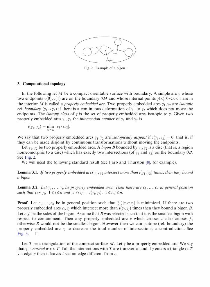
Let g1; g2 be two properly embedded arcs. A bigon B bounded by g1; g2 is a disc (that is, a regionhomeomorphic to a disc) which has exactly two intersections (of g1 and g2) on the boundary @B:See Fig. 2.

We will need the following standard result (see Farb and Thurston [8], for example).

Lemma 3.1. If two properly embedded arcs g1; g2 intersect more than iðg1; g2Þ times, then they bounda bigon.

Lemma 3.2. Let g1;y; gn be properly embedded arcs. Then there are c1;y; cn in general position

such that ciBgi; 1pipn and jci-cjj ¼ iðgi; gjÞ; 1pi; jpn:

Proof. Let c1;y; cn be in general position such thatP

jci-cjj is minimized. If there are two

properly embedded arcs ci; cj which intersect more than iðgi; gjÞ times then they bound a bigon B:

Let e; f be the sides of the bigon. Assume that B was selected such that it is the smallest bigon withrespect to containment. Then any properly embedded arc c which crosses e also crosses f ;otherwise B would not be the smallest bigon. However then we can isotope (rel. boundary) theproperly embedded arc ci to decrease the total number of intersections, a contradiction. SeeFig. 3. &

Let T be a triangulation of the compact surface M: Let g be a properly embedded arc. We saythat g is normal w.r.t. T if all the intersections with T are transversal and if g enters a triangle tAT

via edge e then it leaves t via an edge different from e:

a bigon

Fig. 2. Example of a bigon.

Lemma 3.3. Let T be triangulation of a surface M: Let g be a non-trivial properly embedded arc.Then there is cBg which is normal w.r.t. T :

Proof. Let cBg which minimizes the number of intersections with T : If c enters and leaves tAT

through the same edge e then the number of intersections of c with T can be reduced (since g isassumed to be non-trivial), a contradiction. &

Given a properly embedded arc g which is normal w.r.t. T we can label each edge of thetriangulation with the number of intersections of g with that edge. In each triangle the labels of itsedges determine the behavior of the curve inside the triangle up to isotopy (here we make use ofthe fact that g is normal w.r.t. T and that g is not self-intersecting). Hence the numbering on T

determines the isotopy class of g: We let the size of the representation be the total bitlength of thelabels. An isotopy class may have many different representations. See Fig. 4.

Call a numbering c : ET-N of T valid if there is a properly embedded arc g in general positionw.r.t. T which intersects each eAT ; cðeÞ times. We say that g realizes the numbering c:

Let c be a valid numbering. The sum of the labels of edges from ET-@M is 2: For each triangletAT the labels a; b; c of edges of t satisfy a þ bXc; a þ cXb; b þ cXa and a þ b þ c is even. Theseconditions are necessary for validity, but not sufficient. Call a labeling satisfying these conditionssemi-valid. Any semi-valid labeling defines a properly-embedded arc and a (possibly empty) set ofclosed curves.

We associate the following system of word equations with the triangulation T : The system willemulate the behavior of a set of labeled curves on M: We assume that the curves do not intersect.For each oriented edge ðu; vÞAT there is a variable xu;v encoding the order in which the curves

intersect on ðu; vÞ: Let tAT be a triangle with vertices u; v;w: We add six variables yt;u; yt;v; yt;w;yu;t; yv;t; yw;t as shown in Fig. 5. For example, the variable yt;u encodes the segments of curves

between the oriented edges ðw; uÞ and ðv; uÞ: We have the following equations:

xu;v ¼ yu;tyt;v; xv;u ¼ yv;tyt;u;

xv;w ¼ yv;tyt;w; xw;v ¼ yw;tyt;v;

xu;w ¼ yu;tyy;w; xw;u ¼ yw;tyt;u:

1

1

111

1

11

1

1

00

00

00

0 1

10

2

Fig. 4. Example of a numbering.

Fig. 3. Decreasing the number of intersections.

Note that if we know the lengths of the x variables, then we can calculate the lengths of the othervariables, for example jyu;tj ¼ ðjxu;vj þ jxu;wj jxv;wjÞ=2:

Lemma 3.4. Given a numbering c : ET-N we can test whether c is valid in polynomial time.

Proof. We first verify that c is semi-valid, and reject c if it is not.Let S ¼ fa; bg: Take the set of equations associated with T over S: For each e ¼ ðu; vÞAET

specify jxu;vj ¼ cðeÞ: For each edge e ¼ ðu; vÞAET-@M we specify xu;v ¼ bcðeÞ:We claim that if c is valid then the system of equations has a unique solution. Take the

properly embedded arc g which realizes c: Number the intersections of g with T in the order inwhich they occur on g: Each intersection corresponds to a position in some variable. By induc-tion on the number of intersections it follows that each position in every variable is forcedto be b:

On the other hand let us assume that c is not valid. Because it is semi-valid, there is a solution tothe set of word equations. However, a lexicographically smallest solution will now contain theletter a (corresponding to the closed curves, disconnected from the endpoints labeled b). Becauseof Theorem 2.2 we can compute the lexicographically least solution in polynomial time, and—using Lemma 2.4—check that it does not contain any occurrences of a:

Thus by solving the system, we can check whether c is valid. &

Lemma 3.5. Let g1; g2 be properly embedded arcs given by valid numberings c1; c2: If g1; g2 do notintersect then we can verify that iðg1; g2Þ ¼ 0 in polynomial time. Furthermore if the verification

concludes that iðg1; g2Þ ¼ 0; then g1 and g2 are isotopically disjoint.

Proof. Let S ¼ fa; bg: Take the set of equations associated with T over S: For each e ¼ ðu; vÞAET

specify jxu;vj ¼ c1ðeÞ þ c2ðeÞ: For each edge e ¼ ðu; vÞAET-@M we specify xu;v ¼ w where w

represents the order in which g1 and g2 occur on e:Let h be a solution of the system. Assume that the number of occurrences of a in hðxu;vÞ is

c1ðu; vÞ and xu;v ¼ xRv;u for all ðu; vÞAET : Then g1 and g2 are isotopically disjoint.

w

x

x

y

y

yu,v

u,t

t,v

v,t

v,w

u

v

Fig. 5. The variables for a triangle t:

If g1 and g2 are disjoint then the system has a unique solution h: The proof is analogous to theargument in the proof of Lemma 3.4.

Since the solution h is unique we can find LZðhÞ in polynomial time by Theorem 2.2. For each

e ¼ ðu; vÞAE we verify that the number of occurrences of a in hðxu;vÞ is c1ðeÞ; and xu;v ¼ xRv;u using

Lemmas 2.3 and 2.4. &

4. Weak realizability

In this section we show that the weak realizability problem can be decided in NP: We firsttranslate the weak realizability problem into a more topological version (Proposition 4.2), so wecan apply the topological results.

At this point we need the following bound on the number of intersections in a drawing of aweak realization with the smallest number of intersections.

Theorem 4.1 (Schaefer and Stefankovic [24]). Let G be a graph with m edges, RDðE2Þ such that

ðG;RÞ is weakly realizable, and let D be a weak realization of ðG;RÞ with the minimal number ofintersections. Then for any edge eAG there are less than 2m intersections on the curve realizing e in D:

With this bound we can derive an upper bound on intersections in the topological variant ofweak realizability (Lemma 4.3). We can then apply the results on numberings from Section 3 tofinish the proof (Theorem 4.4).

To apply our topological results, we define a topological variant of the weak realizabilityproblem. Let G ¼ ðV ;EÞ be a graph. Let M be the surface obtained from the plane by drilling jV jholes, each hole labeled by a vertex of G: Let RDðE

2Þ: A set S of properly embedded arcs on M is

called a weak realization with holes of ðG;RÞ if for each e ¼ fu; vgAE there is a properly embeddedarc in S connecting hole u to hole v and if ðe; f ÞeR then the properly embedded arcs e; f areisotopically disjoint.

Given a weak realization D we can drill small holes in place of the vertices to obtain a weakrealization with holes. Given a weak realization with holes, by Lemma 3.2 there is a weakrealization with holes in which for ðe; f ÞeR the properly embedded arcs e; f are disjoint, ratherthan just isotopically disjoint. Contracting the holes we obtain a weak realization of ðG;RÞ: Thisproves the following proposition.

Proposition 4.2. ðG;RÞ is weakly realizable iff there is a weak realization with holes.

Lemma 4.3. Let G be a graph with m edges and n vertices. Assume that ðG;RÞ has a weak

realization with holes. Let M be the surface obtained from the plane by drilling jV j holes. Let T be aminimal triangulation of M: Then there is a weak realization with holes of ðG;RÞ in M such that

there are at most 212nþm intersections on each edge of T :

Proof. We can construct a triangulation T with 3n vertices, using 3 vertices for each boundarycomponent (hole) and no vertices in the interior of the surface. By a simple application of Euler’sformula, T has 9n 6 edges.

Consider the following weak realization problem. Graph H has vertices VH ¼ VT,VG: Wealso include all edges from G and T in H; so that ET,EGDEH : Moreover, there are edgesconnecting vAVG to all vertices of T which lie on the boundary of the hole labeled v: The pairs Pof edges which are allowed to intersect are the following:

* All pairs in R are allowed to intersect.* For every vAG fix an edge evAT on the boundary of the hole labeled v: Then ev is allowed to

intersect edges in EG incident to v:* Any edge in T which is not on the boundary @M can intersect any edge in EG:

By construction, ðG;RÞ is weakly realizable iff ðH;PÞ is weakly realizable.Consider the realization of H with the smallest number of intersections. By Theorem 4.1 there is

a realization of H such that along each edge there are at most 2jEH jp212nþm intersections. &

Theorem 4.4. The weak realizability problem is in NP:

Proof. Let ðG;RÞ be an instance of the weak realizability problem with n ¼ jVGj; and m ¼ jEGj:We will show that deciding whether ðG;RÞ has a weak realization with holes lies in NP: SinceProposition 4.2 established the equivalence of weak realizability and weak realizability with holes,this proves the result.

Suppose ðG;RÞ has a weak realization with holes. Let T be a minimal triangulation of thesurface M: Lemma 4.3 implies that there is a weak realization with holes in which every edge of T

is intersected at most 212nþm times. Hence every edge e of G can be represented by an arc g with a

numbering cg : ET-f0;y; 212nþmg: Furthermore, by Lemma 3.2, we can assume that two arcs g1and g2 representing two edges ðe; f ÞeR are disjoint. To verify weak realizability with holes of

ðG;RÞ it is therefore sufficient to guess, for each edge e of G; a numbering ce : ET-f0;y; 212nþmgof T (note that the numbering has size polynomial in G). We then check that all guessednumberings are valid, and verify that for every ðe; f ÞeR the curves representing e and f areisotopically disjoint. Both tasks can be performed in polynomial time (Lemmas 3.4 and 3.5). Sincethe verification succeeds if and only if ðG;RÞ has a weak realization by holes, this implies thatweak realizability with holes can be verified in NP: &

5. String graphs on surfaces and trace monoids

In proving Theorem 4.4 on string graphs in the plane we only once used the fact that the surfacewas a plane, namely when we applied Theorem 4.1 which has been shown for the plane only. Therest of the proof—Lemma 3.2 and the assumption that we can triangulate the surface in Theorem4.4—hold true for any compact surface. However, we do not currently have any good bounds onthe number of intersections necessary to realize a string graph in a surface other than the plane,since the methods in the proof of Theorem 4.4 do not seem to apply to surfaces of higher genusthan the plane. We make the following conjecture extending the original conjecture of Kratochvıland Matousek [16].

Conjecture 5.1. A graph that has a weak realization on any compact surface can be realized on that

surface with at most Oð2nkÞ intersections for some fixed k40:

If the conjecture were true, then the proof of Theorem 4.4 would generalize to compactsurfaces of any genus, and we would obtain that the weak realization problem, and thereforethe string graph problem, are in NP for arbitrary orientable surfaces. Meanwhile we can

only state the following result, for which we let cSs ðGÞ be the generalization of csðGÞ to a

surface S:

Theorem 5.2. String graphs can be recognized in NTIMEðlog cSs ðnÞÞ on a compact surface S; where

n is the number of vertices of the string graph.

In the absence of any upper bound on cSs for any surface other than the plane this means that

we face the question of decidability anew. This time we use a different approach already suggestedby the proof of Theorem 4.1. We will use the connection between weak realizability and equationson words. Words over an alphabet form a monoid, with concatenation as the operation on themonoid.

Our successful use of monoids in the proof of Theorem 4.4 relied on three facts: theexponential upper bound on cw which allowed us to guess the lengths of the variablesinvolved in the word equations; the fact that we only had to verify arcs that do not inter-sect making it possible to phrase the problem as an equation between words; and that wecould assume the solution to be unique, resolving the question of how to deal with the

operator �R:Since none of these conditions are guaranteed in the general case, we need stronger results on

word equations:

* we cannot make assumptions on the lengths of variables,* arcs can intersect, that is some pairs of letters must be allowed to commute, and* we have to allow equations using �R:

The main problem here is the second item: allowing selected pairs of letters to commute. Let F bethe free monoid over the alphabet G; and I be an irreflexive, symmetric relation on G: I defines an

equivalence relation �I on F by taking the transitive and reflexive closure of �1I which is defined

as u �1I v if and only if u ¼ xaby; and v ¼ xbay for some ða; bÞAI : That is, �I identifies words in F

that can be obtained from each other by permuting pairs of letters in I : The monoid MðG; IÞ ¼F= �I is called a trace monoid over alphabet G with independence relation I : Intuitively, we equatewords over G modulo the allowed commutations in I :

Trace monoids have been under investigation for a while, and Matiyasevich showed in 1996that the solvability of equations in trace monoids is decidable [5]. For our purpose we need a

stronger result that allows equations with the operator �R: This result was only recently obtainedby Diekert and Muscholl [7], building on work by Diekert et al. [4]. For our purposes, asimplified version of this result is sufficient. Note that our translation from weak realizabilityto word equations resulted in a quadratic system; that is, every variable occurred at most

twice. For these systems, Diekert showed the following result, whose proof can be found in theappendix.

Theorem 5.3 (Diekert [3]). The solvability of quadratic systems of word equations in trace monoids

with involution can be decided in PSPACE: Furthermore, if the system is solvable, there is a solutionof at most double-exponential length.

We can apply this result to the string graph problem on an arbitrary compact surface S: Ourgoal is to decide whether ðG;RÞ is weakly realizable in S: We add jGj holes to the surface S; andfix a triangulation T of the resulting surface. As we did in the proof of Lemma 3.4 we introduce avariable xu;v for each edge ðu; vÞ in T ; and variables yt;u; yt;v; yt;w; yu;t; yv;t; yw;t for each triangle t in

T : (See Fig. 5.) We require that xu;v ¼ yu;tyt;v; xv;u ¼ yv;tyt;u; xv;w ¼ yv;tyt;w; xw;v ¼ yw;tyt;v; and

xu;w ¼ yu;tyy;w; xw;u ¼ yw;tyt;u: Furthermore, we ask that yt;u ¼ yRu;t for all vertices u; and triangles t

of T : We associate each vertex h of G arbitrarily with an edge ðu; vÞ of T on the boundary of Ssuch that no two vertices are associated with edges that share a vertex. Let G ¼ fe: e is an edge ofGg: For each vertex h of G; let EðhÞ be the set of edges that contain h: For each h fix an arbitrarypermutation ph of these edges (as letters in G), and add the equation xu;v ¼ eh to the system, where

ðu; vÞ is the edge associated with h: Consider the trace monoid over G with independence relationR: We claim that the set of equations we built has a solution in that trace monoid, if and only ifðG;RÞ is weakly realizable in S: This, however, is immediate, since the allowable crossings in thetrace monoid correspond to the allowed intersections in R: We also observe that every variableoccurred at most twice, making the system quadratic.

Corollary 5.4. The string graph problem, and the weak realizability problem are decidable in

PSPACE on any compact surface. Furthermore, cSs ðGÞ ¼ Oð22polyðjGjÞÞ:

The upper bound on cSs is one exponential jump beyond Conjecture 5.1, it will probably be hard

to remove this jump, since this would have consequences for word and trace equations (seeAppendix A).

6. Conclusion

We now have three essentially different proofs of the decidability of string graphs. Pach andToth [21] solved the problem using purely graph theoretical and topological methods. At the sametime Schaefer and Stefankovic [24] settled the problem based on the idea of looking atintersections along edges as words, and looking for avoidable patterns in words. In Section 5, wemodified this idea and showed that we can easily rephrase the realizability of string graphs—evenon arbitrary surfaces—as a solvability problem over trace monoids with involutions, a problemshown decidable by Diekert and Muscholl [7]. While this has led us to a better understanding ofthe connections between word equations and graph drawing, we feel that we still have not beenable to lay our hands on the combinatorial and topological heart of the string graph problem. It isstill as mysterious as it used to be.

Acknowledgments

We thank Volker Diekert and Geza Toth for helpful discussions, and Volker Diekert forcustom-tailoring Theorem 5.3 for our purposes, and allowing us to include it in the paper.

Appendix A. Quadratic equations

A word or trace equation is called quadratic, if every variable occurs at most twice.Quadratic equations are significantly easier to handle than the general case, and often bettercomplexity bounds are available. Compare, for example, Theorem 2.2 to the followingresult.

Proposition A.1 (Robson and Diekert [23]). Let u ¼ v be a quadratic word equation with lengthsspecified by a function f : In linear time we can decide whether the equation has a solution, and

produce a most general solution to the equation (in the form of a straight line program).

Diekert [3] has pointed out that the proof of this result can easily be extended to include

equations that contain the involution operator �R (which reverses a word). Using thisextended result we could slightly simplify the proof of Lemma 3.5, and reduce the comp-lexity of the verification step of the NP-algorithm in Theorem 4.4 from polynomial time tolinear time.

More importantly for our purposes, a similar result can be obtained for quadratic traceequations. The original version of this paper made use of a solution to general trace equationswith involution due to Diekert and Muscholl, building on work by Diekert et al. [4,5].

Proposition A.2 (Diekert and Muscholl [7]). The solvability of systems of equations in tracemonoids with involution is decidable.

A close look at the decision procedure showed that it could probably be made to run inEXPSPACE: However, it turns out that the special case of quadratic trace equations, even withinvolution, is much simpler, and solvability can be decided in PSPACE: This unpublished result isdue to Volker Diekert who generously allowed us to include a proof of it in this paper. We repeatthe statement of Theorem 5.3 from Section 5.

Theorem 5.3 (Diekert [3]). The solvability of quadratic systems of word equations in trace monoids

with involution can be decided in PSPACE: Furthermore, if the system is solvable, there is a solutionof at most double-exponential length.

Theorem 5.3 is not believed to be optimal. The problem is known to be NP-hard, and Robsonand Diekert [23] conjectured the variant for words to be in NP:

For the proof we need the Levi-lemma for traces, a standard tool in the theory of traces due toCori and Perrin [6,19]. We do not include its proof. For a word w over an alphabet G; letalphðwÞDG denote the set of letters occurring in w:

Lemma A.3. Let M ¼ MðG; IÞ be a trace monoid over alphabet G with independence relation I : If

x; u; y;w are traces in M; then xu ¼ yw if and only if there are traces p; r; s; and q such that x ¼ pr;y ¼ ps; u ¼ sq; w ¼ rq and alphðrÞ alphðsÞDI :

For two traces r and s we write ðr; sÞAI if alphðrÞ alphðsÞDI ; that is, every letter in rcommutes with every letter in s: In this case alphðrÞ and alphðsÞ have to be disjoint, since I isirreflexive.

Proof of Theorem 5.3. Fix the trace monoid M ¼ MðG; IÞ; and the set O of variables. We aregiven a quadratic system of trace equations. A solution to the system is a mapping s :O,G-G�

which fulfills all equations, and such that s is the identity on G:For each variable x in O the algorithm guesses a set aðxÞDG for the letters in sðxÞ of a solution

s; if there is one. Since PSPACE is closed under nondeterminism, and aðxÞ has size at most G; thiscan be done in PSPACE: In the following we assume we are looking at a fixed a :O-2G:

The weight mðuÞ of a word u ¼ u1?ukAðG,OÞ� is defined asPk

i¼1 jaðuiÞj; where we let aðaÞ ¼fag for all aAG: We extend the notion of weight to equations, and system of equations by addingthe weights of all parts. The weight of a system is a measure of how much space the algorithmneeds to store the all information it needs about the system of equations. Note that initially theweight of a system can be at most quadratic in the size of the input. In each step of the algorithmwe guarantee that the weight of the system will not increase. Hence the algorithm requires onlypolynomial space.

The weight upper bound will not guarantee the algorithm’s termination. For this we need adifferent measure. Suppose a system of equations has a solution s :G,O-G�: We can define the

length of an equation u1?un ¼ v1?vm with regard to s asPn

i¼1 jsðuiÞj þPm

i¼1 jsðviÞj; and the

length of a system of equations with regard to s as the sum of the lengths of all its equations (withregard to s). The length of a system of equations then is the minimum of all lengths over allpossible solutions s: If there is no solution, we let the length be infinite.

We will show that the algorithm decreases the length of the system by at least 1 in each step, andtherefore it has to terminate. Since we guarantee that the weight of the system does not increase,and that weight initially is polynomial, we will be able to conclude that the algorithm runs inpolynomial space.

Consider an equation

xu ¼ y1?yk ðA:1Þ

with x; y1;y; ykAG,O and uAðG,OÞ�: Choose i maximal such that ðx; y1?yi 1ÞAI ; and let

y ¼ yi: (Note that we can assume that i 1ok: if ðx; y1?ykÞAI ; then alphðxÞ-alphðy1?ykÞ ¼ |in which case we can conclude that there is no solution to the system.) Eq. (A.1) then turns into

xu ¼ vyw; ðA:2Þ

where x; yAG,O; v;wAðG,OÞ�; and ðx; vÞAI : Since alphðxÞ-alphðvÞ has to be empty (becauseðx; vÞAI), x has to be a prefix of yw: By Levy’s Lemma, we know that there are traces p; r; and ssuch that x ¼ pr; and y ¼ ps; where ðr; sÞAI : This allows us to rewrite Eq. (A.2) as

pru ¼ vpsw ðA:3Þ

which is the same as pru ¼ pvsw; since ðp; vÞ has to be in I ; as ðx; vÞ is, and therefore

ru ¼ vsw ðA:4Þ

because we can cancel p: At this point we add new variables r and s to G; and guess aðpÞ; aðrÞ; andaðsÞ such that

aðxÞ ¼ aðpÞ,aðrÞ;

aðyÞ ¼ aðpÞ,aðsÞ;

aðrÞ aðsÞDI :

Since we assumed that i is maximal, we know that p cannot be empty. We distinguish five casesdepending on x and y:

Case 1: x ¼ aAG: In this case p ¼ a and r ¼ e: If yAG; then y has to be a (otherwisethere is no solution), and substituting Eq. (A.1) by Eq. (A.4) reduced the overall weight by 2:Otherwise yAO; and we know that y ¼ as: Hence we can substitute the second occurrence of ywith as: This potentially increases the weight of the system by 1; but since we also replaceEq. (A.1) by Eq. (A.4) (with r ¼ e) reducing the weight by 1; we have not increased the overallweight.

Case 2: y ¼ aAG: Similar to Case 1.Hence, we know that x; yAO:Case 3: x ¼ y: Again, substituting Eq. (A.1) by Eq. (A.4) reduces the weight by 2 (remember

that we removed variables u with aðuÞ ¼ |).

Case 4: x ¼ yR: In this case ps ¼ y ¼ xR ¼ ðprÞR ¼ rRpR: Since s and r do not have any letters in

common (remember that ðr; sÞAI), this is impossible, unless both s ¼ r ¼ e; and therefore x ¼y ¼ p ¼ pR: Since there is always a solution to y ¼ yR; whatever alphðyÞ; this allows us to replaceEq. (A.1) by u ¼ vw; reducing the weight of the system. (There cannot be any other occurrences of

y; since it already appears as y and yR:)

Case 5: x; yAO; and xay; yR: Substitute Eq. (A.1) by Eq. (A.4), and replace the second

occurrence of x (if any) by pr (or rRpR; if it is xR), and the second occurrence of y (if any) by ps (or

sRpR; if it is yR). We changed the overall weight of the system by

2ðjaðxÞj þ jaðyÞjÞ þ 2jaðpÞj þ jaðrÞj þ jaðsÞjp0:

The inequality is true, since aðxÞ-aðyÞ ¼ aðpÞ (r and s being independent), and therefore jaðxÞj þjaðyÞj ¼ jaðxÞ,aðyÞj þ jaðxÞ-aðyÞj ¼ jaðpÞ,aðrÞ,aðsÞj þ jaðpÞjXjaðrÞ ’,aðsÞj þ jaðpÞj ¼ jaðpÞjþjaðrÞj þ jaðsÞj: Therefore, the weight of the system did not increase.

The five cases are exhaustive. Note that in each case the weight of the system did not increase.Furthermore, in all cases the length of the system was reduced by at least 2jpj; since xu ¼ vyw(which is pru ¼ vpsw) is replaced by ru ¼ vsw: Since p cannot be empty, this means the length ofthe system is reduced in every step. Hence, the algorithm has to terminate, either by running into acontradiction, or with the empty system, in which case there is a solution (since the solvability ofthe system remained unchanged). In every step of the algorithm we remove variables x and y from

the system and replace them by pr and ps: Hence jxj þ jyjpjpj þ jrj þ jpj þ jsj which means that inevery step the length of the system at most halves. Since the algorithm takes an exponential

number of steps, this gives us an upper bound of Oð22polyðnÞ Þ on the length of the original system ofequations, showing that there is a solution of double exponential length. &

References

[1] S. Benzer, On the topology of the genetic fine structure, Proc. Nat. Acad. Sci. 45 (1959) 1607–1620.

[2] Z.-Z. Chen, M. Grigni, C. Papadimitriou, Planar map graphs, in: Proceedings of the 30th Annual ACM

Symposium on Theory of Computing (STOC-98), ACM Press, New York, pp. 514–523, 1998.

[3] V. Diekert, Personal communication, 2002.

[4] V. Diekert, C. Gutierrez, C. Hagenah, Existential theory of equations with rational constraints in free groups is

PSPACE-complete, in: Proceedings of the 18th International Symposium on Theoretical Aspects of Computer

Science, STACS 2001, pp. 170–182.

[5] V. Diekert, Y. Matiyasevich, A. Muscholl, Solving trace equations using lexicographical normal forms, in:

Proceedings of the 24th International Colloquium on Automata, Languages and Programming (ICALP’97),

Bologna, Italy, 1997, Springer, Berlin-Heidelberg-New York, pp. 336–346. URL citeseer.nj.nec.com/diekert97-

solving.html.

[6] V. Diekert, Y. Metivier, Partial commutation and traces, in: G. Rozenberg, A. Salomaa (Eds.), Handbook on

Formal Languages, Vol. III, Springer, Berlin-Heidelberg-New York, 1997.

[7] V. Diekert, A. Muscholl, Solvability of equations in free partially commutative groups is decidable, in: ICALP

2001, pp. 543–554.

[8] B. Farb, B. Thurston, Homeomorphisms and simple closed curves, unpublished manuscript, 1991.

[9] M.R. Garey, D.S. Johnson, Crossing number is NP-complete, SIAM J. Algebraic Discrete Methods 4 (3) (1983)

312–316.

[10] L. G-asieniec, M. Karpinski, W. Plandowski, W. Rytter, Efficient algorithms for Lempel-Ziv encoding, in:

Proceedings of SWAT’96, Lecture Notes in Computer Science, Vol. 1097, 1996, pp. 392–403.

[11] R.L. Graham, Problem 1, in: Open Problems at 5th Hungarian Colloquium on Combinatorics, 1996.

[12] M. Grigni, D. Papadias, C. Papadimitriou, Topological inference, in: Proceedings of the 14th International Joint

Conference on Artificial Intelligence, 1995, pp. 901–906.

[13] J. Kratochvıl, String Graphs. I. The number of critical nonstring graphs is infinite, J. Combin. Theory, Series B 52

(1991a).

[14] J. Kratochvıl, String graphs. II. Recognizing string graphs is NP-hard, J. Combin. Theory, Series B 52

(1991b).

[15] J. Kratochvıl, Crossing number of abstract topological graphs, Lecture Notes in Comput. Sci. 1547 (1998)

238–245.

[16] J. Kratochvıl, J. Matousek, String graphs requiring exponential representations, J. Combin. Theory, Series B 53

(1991) 1–4.

[17] M. Lothaire, Algebraic Combinatorics on Words, in: Encyclopedia of Mathematics and its Applications, Vol. 90,

Cambridge University Press, Cambridge, 2002.

[18] J. Matousek, J. Nesetril, R. Thomas, On polynomial time decidability of induced-minor-closed classes, Comment.

Math. Univ. Carolin. 29 (4) (1988) 703–710.

[19] A. Mazurkiewicz, Introduction to trace theory, in: V. Diekert, G. Rozenberg (Eds.), The Book of Traces, World

Scientific, Singapore, Chapter 1, 1995, pp. 3–41.

[20] J. Pach, G. Toth, Which crossing number is it anyway?, J. Combin. Theory, Series B 80 (2000) 225–246.

[21] J. Pach, G. Toth, Recognizing string graphs is decidable, in: P. Mutzel (Ed.), Graph Drawing 2001, Lecture Notes

in Computer Science, Springer, Berlin, pp. 247–260.

[22] W. Plandowski, W. Rytter, Application of Lempel–Ziv encodings to the solution of words equations, Automata,

Languages and Programming (1998), 731–742.

[23] J.M. Robson, V. Diekert, On quadratic word equations, in: C. Meinel et al. (Eds.), 16th STACS, Trier, 1999,

Lecture Notes in Computer Science, Vol. 1563, Springer-Verlag, Berlin, pp. 217–226.

[24] M. Schaefer, D. Stefankovic, Decidability of String Graphs, in: Proceedings of the 33rd Annual ACM Symposium

on Theory of Computing (STOC-2001), pp. 241–246.

[25] F.W. Sinden, Topology of thin film circuits, Bell System Tech. J. 45 (1966) 1639–1662.

[26] M. Thorup, Map graphs in polynomial time, in: IEEE Symposium on Foundations of Computer Science,

pp. 396–405, 1998.