J. Fluid Mech. (2001), vol. 431, pp. 91–133. Printed in the United Kingdom

c© 2001 Cambridge University Press

91

Receptivity of boundary layers with distributedroughness to vortical and acoustic disturbances:

a second-order asymptotic theory andcomparison with experiments

By X U E S O N G W UDepartment of Mathematics, Imperial College, 180 Queens Gate, London SW7 2BZ, UK

(Received 11 February 2000 and in revised form 19 September 2000)

This paper investigates the receptivity of boundary layers due to distributed roughnessinteracting with free-stream disturbances. Both acoustic and vortical perturbationsare considered. An asymptotic approach based on the triple-deck formulation hasbeen developed to determine the initial amplitude of the Tollmien–Schlichting wave tothe O(R−1/8) accuracy, where R is the global Reynolds number. In the case of vorticaldisturbances, we show that the dominant contribution to the receptivity comes fromthe upper deck as well as from the so-called edge layer centred at the outer reach ofthe boundary layer. It is found that for certain forms of disturbances, the receptivityis independent of their vertical structure and can be fully characterized by their slipvelocity at the edge of the boundary layer. A typical case is the vortical disturbancein the form of a convecting wake, for which the same conclusion as above has beenreached by Dietz (1999) on the basis of measurements. Our theoretical predictionsare compared with the experimental data of Dietz (1999), and a good quantitativeagreement has been found. Such a comparison is the first to be made for distributedvortical receptivity. Further calculations indicate that the vortical receptivity in generalis much stronger than was suggested previously. In the case of acoustic disturbances,it is found that our first-order theory is in good agreement with experiments as wellas with previous theoretical results. But the second-order theory over-predicts, andthe possible reasons for this are discussed.

1. IntroductionOne of the fundamental questions concerning laminar–turbulent transition in the

boundary layer is the so-called receptivity (Morkovin 1969; Reshotko 1976), whichrefers to the process whereby external disturbances present in the environment (e.g.in a free stream and/or on a wall) excite internal oscillations within the boundarylayer. When the free-stream turbulence level is low (below a few per cent), thedominant boundary-layer response is Tollmien–Schlichting (T-S) waves. But high-level free-stream turbulence tends to generate broad-band low-frequency motions,i.e. the so-called Klebanoff modes, which undergo transient growth and may leadto secondary instability. The present paper is concerned with the generation of T-Swaves. It is well-known that in a uniform free stream a general unsteady small-amplitude perturbation can be expressed as a superposition of acoustic and vorticalmodes (and entropy modes if the fluid is compressible) (Kovasznay 1953). The formerrepresents sound waves, while the latter is the vorticity fluctuation being convected

92 X. Wu

by the free stream and is often referred to as a convecting gust. Because the lengthand time scales of each mode do not satisfy the dispersion relation of T-S waves,neither of them alone can excite any T-S waves. Therefore the first task of receptivitystudy is to identify the scale-conversion mechanisms, which ‘tune’ the time and/orlength scales of the external disturbance so as to match those of the T-S waves. Thesecond task of course is to calculate the initial amplitude or equivalently the so-calledcoupling coefficient.

The major breakthrough came with the seminal papers by Goldstein (1983, 1985)and Ruban (1984), in which several important scale-conversion mechanisms havebeen identified and quantified. The first of these involves an acoustic disturbance (i.e.a sound wave) interacting with the non-parallel mean flow near the leading edgeto excite the so-called Lam–Rott eigensolution, which then undergoes wavelengthshortening and finally turns into a T-S wave near the lower branch of the neutralcurve (Goldstein 1983). This receptivity, however, turns out to be somewhat weakbecause the wave may experience considerable decay before reaching its neutral-stability point. A more efficient mechanism was identified independently by Goldstein(1985) and Ruban (1984). It involves the interaction between a sound wave and arapidly varying mean flow, induced by a small localized roughness on the wall, orby a sudden curvature change (such as the one that occurs at the juncture of theleading-edge ellipse and the straight portion of the plate; see Goldstein & Hultgren1987). The resulting unsteady forcing can excite a T-S wave if the frequency of thesound and the length scale of the local mean flow are comparable with those of theT-S wave. In the framework of triple-deck theory, the leading-order interaction takesplace in the lower deck since both the steady and unsteady perturbations concentratein that region.

A somewhat similar scale-conversion mechanism operates to generate a T-S wavewhen a vortical disturbance interacts with a roughness. This has been analysed byDuck, Ruban & Zhikharev (1996), again using a triple-deck formulation. See alsoKerschen (1991). The main difference from the acoustic disturbance is that a vorticaldisturbance does not penetrate into the boundary layer in the sense that its signatureis exponentially small there (Gulyaev et al. 1989). Thus the dominant interactionnow occurs in the upper deck (and also in the so-called edge layer centred at theouter reach of the boundary layer). Since the mean-flow distortion is weaker inthe upper deck, the coupling coefficient is found to be a factor R−1/8 smaller thanthat in the corresponding acoustic case, where R is the global Reynolds number.Choudhari (1996) studied the same kind of interaction between a three-dimensionalgust and a localized roughness using an approach based on the Orr–Sommerfeld (O-S)equations. His calculations showed that the lower-frequency components of the gustare a more effective T-S wave generator. A quantitative comparison between theoryand experiments has not been possible until recently, because earlier experimentalinvestigations (e.g. Kendall 1985, 1990) were conducted in uncontrolled conditions andmost information was qualitative. Controlled experiments have been carried out onlyrecently by Dietz (1996, 1998, 1999), who successfully introduced a single-frequencyvortical disturbance, a convecting wake, by vibrating a ribbon in the oncoming freestream. His experiments provide for the first time quantitative data about the initialamplitude of the T-S waves due to a convecting gust interacting with a wall roughnesselement. In the case of localized roughness, Dietz compared his experimental data withthe calculations of Choudhari (1996) and also with the prediction by an asymptoticformula of Kerschen (1991). The agreement with the former was reasonable, butthe latter turned out to be just about 40% of the measured value. Nevertheless, the

Receptivity of boundary layers with distributed roughness 93

evidence is strong enough to suggest that the basic mechanism proposed in previoustheoretical studies is a correct one.

Recently, Wu (1999) proposed a mechanism which is distinct from those mentionedabove. It involves the direct interaction between a vortical disturbance and a soundwave of suitable frequencies and wavenumbers so as to achieve scale conversion.Unlike the mechanism in the Goldstein–Ruban theory, the conversion of the externalscales does not require any form of non-homogeneity on the wall or in the mean flow,and thus operates even in the simplest flows such as the flat-plate boundary layer.

In addition to the localized roughness, the receptivity due to distributed rough-ness has also received considerable interest. It has been suggested that this type ofroughness is more representative of the practical situation. In theoretical studies, adistributed roughness is conveniently modelled by a wavy wall, while in laboratories itis simulated by arrays of equally spaced isolated roughness elements, placed near thelower branch of the T-S waves that are to be excited (Wiegel & Wlezien 1993; Dietz1999). Experiments show that the receptivity increases with the number of roughnesselements N, but approaches a limit as N becomes sufficiently large (N = 9 ∼ 13). Thefinal limit corresponds to the case of an infinite wavy wall, and is about one order ofmagnitude larger than the localized receptivity.

The coupling coefficient of distributed receptivity has been computed by severalauthors. In the case of an acoustic disturbance, Choudhari (1993) treated the contri-bution from the distributed roughness as a superposition of that from isolated ones,an idea originated from the work of Tam (1981). Choudhari’s analysis is based onthe finite-Reynolds-number approach, developed previously by Choudhari & Streett(1992) and Crouch (1992a) for the localized receptivity and by Russian researchers (seee.g. Zhigulev & Tumin 1987). A somewhat different finite-Reynolds-number formula-tion was adopted by Crouch to study the distributed receptivity to acoustic (Crouch1992b) as well as vortical disturbances (Crouch 1994). The key ‘device’ to determinethe T-S waves is an inhomogeneous amplitude equation. This equation, however, wasderived in a rather ad hoc manner, without making use of a superposition principle(as Choudhari 1993 did) or a solvability condition. A feature of some concern is thatin the case of exact resonance, the forcing term in the amplitude equation exhibits asingularity, a second-order pole, at the neutral point of the T-S wave.

In this paper, we shall investigate the distributed receptivity using the high-Reynolds-number approach. The present work was motivated by two facts. Firstit is desirable to provide a self-consistent mathematical description of the distributedreceptivity, in parallel to the work of Goldstein (1985), Ruban (1984) and Duck et al.(1996) for the localized roughness. For the distributed receptivity, the non-parallel-flow effect associated with the streamwise variation of the growth rate of the T-Swaves plays a key role. In particular, the magnitude of the generated T-S wave is di-rectly related to this effect. This crucial issue can be addressed satisfactorily only in anasymptotic framework. Moreover, in the case of vortical disturbances, the non-paralleleffect associated with the thickening of the boundary layer appears at leading orderin the edge layer. This effect is completely ignored by the calculations based on theO-S equations, but can be properly taken into account by the high-Reynolds-numberapproach.

Secondly, for both the acoustic and vortical disturbances, there are well-documentedexperimental data, notably Dietz (1999) for the vortical receptivity and Wiegel &Wlezien (1993) for the acoustic receptivity. It is now possible to make a detailedquantitative comparison between the theory and laboratory measurements. For thispurpose, the asymptotic theory will be extended to the second order, by including

94 X. Wu

the O(R−1/8) correction. Naturally one may be concerned with whether or not theasymptotic approach will be accurate enough for the moderate Reynolds numbers,given that it does not predict the neutral Reynolds number and growth rate accurately.The work of Terent’ev (1981) demonstrates that this approach can be used effectivelyto study the excitation of T-S waves despite the deficiency mentioned above. Theview that the asymptotic approach gives a more accurate prediction for receptivitythan for the dispersion was reaffirmed by Choudhari & Streett (1992). Indeed, ourfinal results, (3.124) and (4.38), show that the amplitudes of the T-S waves are notsensitive to the inaccuracy in the predicted neutral Reynolds number.

It should be remarked that the literature on boundary-layer receptivity is ratherextensive. Here we have mentioned the contributions that are most relevant to thepresent work. A more detailed survey was given in a recent paper (Wu 1999), andreferences to Russian literature on this subject can be found in Duck et al. (1996).

The rest of the paper is organized as follows. In § 2, as a first step in formulatingthe problem, the basic mechanism of the distributed receptivity is described in fairlygeneral terms. The relevant scalings are then introduced so as to develop an asymptotictheory using the triple-deck framework. A wavy wall is used as an idealized modelof distributed roughness. The solution of the mean-flow distortion is obtained upto O(R−1/8). The receptivity to a vortical disturbance is analysed in § 3. In order tomaintain maximum generality, the analysis is carried through without specifying thevertical structure of the gust. The dominant contribution to the receptivity comes fromthe upper deck as well as the edge layer. The interactions in these two regions areanalysed in § 3.1 and § 3.2 respectively. The main layer acts to facilitate the pressure–displacement interplay between the upper and lower decks as in the standard tripledeck, and the solution is given in § 3.3. The forcing from the upper and edge layers istransmitted to the lower deck and results in inhomogeneous systems, the solvabilityconditions of which give rise to the amplitude equations. In § 3.5, we show that thesolutions to these equations can be used to determine the T-S wave amplitude upto O(R−1/8) accuracy. We demonstrate that in certain conditions, the receptivity isindependent of the vertical structure of the gust. Appropriate coupling coefficientsare then defined to quantify the receptivity. In §4, we investigate the receptivity to anacoustic perturbation. The leading-order contribution is from the lower deck (§ 4.3).But there is an O(R−1/8) contribution from both the upper and main layers, and theseare analysed in § 4.1 and § 4.2. The required amplitude equations are derived in § 4.3.Numerical solutions are presented in §5, where the theoretical results are comparedwith the relevant experiments as well as with previous calculations. The conclusionsand implications of the present study are discussed.

2. Formulation and scalingsWe consider the two-dimensional incompressible boundary layer over a semi-infinite

wavy wall. The oncoming flow is assumed to be uniform with velocity U∞, perturbedby small-amplitude disturbances, which will be specified later. We define the Reynoldsnumber

R = U∞l/ν, (2.1)

where l is the typical distance from the leading edge to the location where thereceptivity commences, and ν is the kinematic viscosity.

The flow is to be described in the Cartesian coordinate system (x, y, z) with its originat the leading edge, where x and y are along and normal to the mean position of the

Receptivity of boundary layers with distributed roughness 95

wall respectively, and z is in the spanwise direction; x and z are non-dimensionalizedby l and y by lR−1/2. The time variable t is normalized by l/U∞. The velocity (u, v, w)is non-dimensionalized by U∞, while the non-dimensional pressure p is introduced bywriting the dimensional pressure as (p∞ + ρU2∞p), where p∞ is a constant and ρ is thefluid density.

The basic mechanism of the distributed receptivity is well understood from thephysical point of view, and can be explained in fairly general terms as follows.Suppose first that the dispersion relation of the T-S wave is

∆(ωTS , αTS ; x) = 0, (2.2)

which relates the frequency ωTS and the wavenumber αTS at a given location x,the dependence on which is parametric. In general for a given frequency ωTS , thewavenumber αTS = αr + iαi is a complex number except at the neutral position x0.

In the case of an acoustic disturbance, the pressure fluctuation in the free streamdrives an oscillatory flow near the wall. In the incompressible limit, this flow isproportional to e−iωst. On the other hand, the wall roughness induces a steady meanflow proportional to eiαwx, where ωs and αw are the frequency of the sound and thewavenumber of the roughness respectively. The interaction between the two generatesa forcing term proportional to ei(αwx−ωst). Now if

ωs = ωTS , αw ≈ Re (αTS ), (2.3)

the response to the forcing would be similar to, but not exactly the same as, the T-Swave when x 6= x0. But when x ≈ x0, the relations in (2.3) imply that a resonanceoccurs between the forcing and the T-S wave, leading to the generation of the latter.Mathematically, the resonance means that in order for the inhomogeneous system atthe quadratic order to have an acceptable solution, the T-S wave solution must beincluded in the expansion at a suitable lower order.

In the case of a vortical disturbance (gust), the velocity (and vorticity) fluctuation inthe free stream is proportional to exp (i(αcx− ωct)). Since αc = ωc, there is no pressurefluctuation at leading order, and as a result a vortical disturbance does not penetrateinto the boundary layer. But as in the case of the localized receptivity (cf. Duck etal. 1996), an interaction with the mean-flow distortion takes place in the outer reachof the boundary layer, producing a forcing proportional to exp (i(αw + αc)x− iωct). Aresonance occurs in the vicinity of the lower-branch neutral point x0 if

ωc = ωTS , αw + αc ≈ Re (αTS ). (2.4)

It is noted that for a gust or a sound wave of a given frequency, there exists aunique value of αw to satisfy exactly the second relation in (2.3) or (2.4). Conversely,a roughness of a given wavelength requires the gust or sound to have a particularfrequency in order to have an exact resonance. In controlled experiments, one usuallyimposes αw and varies ωc (or ωs) over a range in which the second relation in (2.3)or (2.4) is satisfied only approximately. T-S waves may still be generated in this moregeneral case, but have a reduced magnitude. Such a tuned response to the forcingfrequency is an important feature of the distributed receptivity, and can be describedby introducing an appropriate detuning parameter (see later).

To calculate the coupling coefficient in each case, we shall develop an asymptotictheory based on the triple-deck formalism; so we assume that R 1. For a lower-branch T-S wave, its frequency and wavenumber scale with the Reynolds numberas

ωTS = R2/8ω, αTS = R3/8α.

96 X. Wu

Pre-resonanceregion

Resonance region

Forced responseNearly neutral

T-S wave

Main layer

Upper deck

Free-evolutionregion

T-S wave withO (1) growth

x0

O (R–3/16)

O (R–1/8) Lower deckO [(ln R)1/2]

Edge layer O [(ln R)–1/2]

Figure 1. Illustration of the receptivity process and the flow structure for the vortical receptivity.

Since the generated T-S wave inherits the frequency of the sound wave or gust, wehave

ωs = ωc = ωTS = R2/8ω, αc = R2/8αc.

Though αc ≡ ω, we shall retain the identity of αc for book-keeping purpose. Theresonant condition (2.3) or (2.4) shows that the wavenumber of the wall roughnessmust scale as

αw = R3/8αw.

It is also convenient to introduce the faster variables

t = R2/8t, x = R3/8x, z = R3/8z, (2.5)

and a small parameter

ε = R−1/8.

The important site of the receptivity process is the neutral point x0 of the T-S wave,since the resonance condition can only be met there. Upstream of x0, the quadraticroughness–gust or roughness–sound interaction generates a small-amplitude response,which is regular. But as x0 is approached, the forced response tends to infinity (i.e.becomes singular), and takes on the characteristics of the T-S wave. In order todescribe this crucial process of the forced response evolving into the T-S wave aftergoing through the resonance, it is necessary to consider the O(R−3/16) neighbourhoodof x0, where the non-parallel-flow effect becomes important in the sense that thevariation of both the growth rate and the amplitude occurs at the same scale (Ruban1983, Hall & Smith 1984). We introduce

x1 = (x− x0)/R−3/16. (2.6)

The amplitude of the T-S wave will be a function of x1, and matches to the forcedresponse upstream as x1 → −∞. Sufficiently downstream the T-S wave evolves intothe post-resonance region where it acquires an O(1) growth rate. Thus the wholeprocess consists of three stages as is illustrated in figure 1, the most important ofwhich is the resonance region. The key role of the O(R−3/16) vicinity of the neutralpoint in receptivity was demonstrated in Wu (1999). See also Choudhari (1993).

One may note that the distributed receptivity is quite different from the isolatedreceptivity in terms of physical process as well as the methods used to determine theT-S wave amplitude. An isolated roughness has a continuous spectrum, and wheninteracting with the unsteady disturbances produces a broad-band response in the

Receptivity of boundary layers with distributed roughness 97

boundary layer. The solution for the response can be expressed as a Fourier integral.The amplitude of the T-S wave is obtained directly by evaluating the residue at thesimple pole of the integrand. But for the distributed receptivity, we shall introduce anamplitude function A(x1) say and derive the equation governing A(x1). This procedureis similar to that in Wu (1999).

Now it follows from (2.5) and (2.6) that

∂

∂t→ R2/8 ∂

∂t,

∂

∂x→ R3/8 ∂

∂x+ R3/16 ∂

∂x1

,∂

∂z→ R3/8 ∂

∂z. (2.7)

The mean flow is taken to be the Blasius boundary layer, the profile of which isUB(y). As y → 0,

UB(y)→ λy

where the skin friction

λ = χx−1/2 with χ ≈ 0.332. (2.8)

We further expand λ about x0, the location where the T-S wave becomes neutral,

λ = λ0 + R−3/16λ1x1, with λ1 = − 12χx−3/20 . (2.9)

Since the length scale l (see (2.1)) is taken to be the distance of the neutral point tothe leading edge, x0 will be assigned the value of unity.

For the triple deck to be applicable, the dimensional height of the wall waviness,h∗, must be of O(R−5/8l) or smaller, and so we may write h∗/l = R−5/8h with h = O(1)or smaller. For simplicity, we shall assume that the mean-flow distortion, and thevortical and acoustic disturbances are all of sufficiently small magnitude that theirself-nonlinearities can be ignored. Formally this requires that

h R−1/8, εc R−1/8, εs R−1/8, (2.10)

where εc and εs stand for the amplitudes of the streamwise velocities of the sound andgust respectively. For such small-amplitude waviness, there is no loss of generalityto assume that the distribution of the roughness is purely sinusoidal since a moregeneral periodic pattern can be decomposed into Fourier series. Thus we take thewall position to be given by

y = R−1/8Fwh(eiαwx + c.c.), (2.11)

where Fw is an order-one parameter representing the coefficient of the first term inthe Fourier series, and c.c. stands for complex conjugate.

In order to develop a second-order asymptotic theory which can predict the initialamplitude of the T-S wave with O(R−1/8) accuracy, it is necessary (i) to retain theO(R−1/8) correction to the leading-order forcing, and (ii) to take into account thecorrection arising from the higher-order modification to the dispersion relation of theT-S wave. In particular, the latter solution must be obtained up to O(R−2/8) so thatthe detuning effect can be described to the required order of accuracy.

As the analysis is lengthy, readers who are more interested in the physical mech-anisms and the final quantitative predictions rather than mathematical technicalitiescould go directly to § 3.5 and the end of § 4, where we give the final results, (3.124) and(4.38), the coupling coefficients for the acoustic and vortical receptivities respectively.

98 X. Wu

2.1. The mean-flow distortion

In the main part of the boundary layer, the mean-flow distortion due to the wavywall is a small perturbation to the Blasius profile (UB, R

−1/2VB), that is

(U,V , P ) = (UB + εhUM, R−1/2VB + ε2hVM, ε

2hPM),

where (UM,VM, PM) expand as

UM = U(1)M + εU

(2)M + · · · eiαwx + c.c.+ O(h) . . . ,

VM = V (1)M + εV

(2)M + · · · eiαwx + c.c.+ O(h) . . . ,

PM = P (1)M + εP

(2)M + · · · eiαwx + c.c.+ O(h) . . . .

(2.12)

Here we can ignore the terms proportional to O(h) since h ε as implied by (2.10).It is well known that the leading-order perturbation has the solution

U(1)M = A

(1)MU

′B, V

(1)M = −iαwA

(1)MUB, (2.13)

where the constant A(1)M is to be determined later. The second-order perturbation is

governed by

iαwU(2)M + V

(2)M,y = 0, (2.14)

iαwUBU(2)M +U ′BV

(2)M = −iαwP

(1)M , (2.15)

iαwUBV(1)M = −P (2)

M,y, (2.16)

which are solved to give

V(2)M = −iαwA

(2)MUB + iαwP

(1)M UB

∫ y dy

U2B

, (2.17)

U(2)M = A

(2)MU

′B − P (1)

M

UB

∫ y dy

U2B

′, (2.18)

P(2)M = P

(2)M − α2

wA(1)M

∫ y

0

U2Bdy, (2.19)

where A(2)M and P (2)

M are constants to be found.In the upper deck, where y = R−1/8y, the steady flow can be written as

(U,V , P ) = (1, 0, 0) + ε2h(uM, vM, pM) eiαwx + c.c.,

with

(uM, vM, pM) = (u(1)M , v

(1)M , p

(1)M ) + ε(u(2)

M , v(2)M , p

(2)M ) + · · · . (2.20)

The governing equations for p(j)M and v(j)

M are

p(j)M,yy − α2

wp(j)M = 0, iαwv

(j)M = −p(j)

M,y (j = 1, 2).

It follows that p(j)M = P

(j)M e−αwy and v

(j)M = −iP (j)

M e−αwy . The continuity equation gives

the streamwise velocities u(j)M = −P (j)

M e−αwy . The pressure and vertical velocity in theupper deck match their counterparts in the main layer if

P(1)M = P

(1)M , P

(2)M = P

(2)M − α2

wA(1)M I2, (2.21)

P(1)M = αwA

(1)M , −iP (2)

M = iαwP(1)M J∞ − iαwA

(2)M , (2.22)

where the constants I2, J∞ are defined by (A 3) and (A 5) of Appendix A respectively.

Receptivity of boundary layers with distributed roughness 99

In the lower deck, the appropriate transverse coordinate is

Y = R1/8y.

In terms of Y , the wall position is given as

Y = hFw(eiαwx + c.c.). (2.23)

The solution can be written as

(U,V , P ) = ε(λY , 0, 0, ) + εh(UM, ε2VM, εPM) eiαwx + c.c.

with

(UM, VM, PM) = (U(1)M , V

(1)M , P

(1)M ) + ε(U(2)

M , V(2)M , P

(2)M ) + · · · . (2.24)

Since h 1, the leading-order terms satisfy the linearized boundary-layer equations

iαwU(1)M + V

(1)M,Y = 0, (2.25)

iαwY U(1)M + λV

(1)M = −iαwP

(1)M + U

(1)M,Y Y , (2.26)

where we have used the fact that P (1)M = P

(1)M . The no-slip condition on the wall is

approximated, after linearization, by

U(1)M (0) = −λFw, V

(1)M (0) = 0,

while the matching condition with the main-deck solution is

U(1)M → λA

(1)M as Y →∞.

Solving these equations, we obtain

U(1)M = λFw

1

D(αw)

∫ ζ

0

Ai(ζ) dζ − 1

, (2.27)

P(1)M = P

(1)M = P

(1)M = −α−2

w (iαwλ)5/3Ai′(0)Fw/D(αw), (2.28)

where ζ = (iαwλ)1/3Y , Ai is the Airy function, and

D(αw) =

∫ ∞0

Ai(ζ) dζ + α−3w (iαwλ)

5/3Ai′(0). (2.29)

The second-order correction U(2)M , V (2)

M and P (2)M satisfy

iαwU(2)M + V

(2)M,Y = 0, (2.30)

iαwY U(2)M + λV

(2)M = −iαwP

(2)M + U

(2)M,Y Y . (2.31)

It can be shown that

V(2)M,ζ = C2

∫ ζ

0

Ai(ζ) dζ

with C2 being a constant. Matching V (2)M,ζ with V (2)

M,y in the main part of the boundarylayer yields

C2

∫ ∞0

Ai(ζ) dζ = −(iαwλ)2/3A

(2)M − P (1)

M J0

, (2.32)

100 X. Wu

with J0 defined by (A 4). The no-slip condition on the wall implies V (2)M,Y Y Y (0) = α2

wP(2)M ,

i.e.

C2Ai′(0) = α2w(iαwλ)

−1P(2)M . (2.33)

It follows from (2.21)–(2.22) and (2.32)–(2.33) that

P(2)M = −αwP

(1)M

D(αw)

α−3w (iαwλ)

5/3Ai′(0)(J∞ − J0) + I2

∫ ∞0

Ai(ζ) dζ

, (2.34)

P(2)M = −α−2

w (iαwλ)5/3P

(1)M (J∞ − J0 − I2)/D(αw), (2.35)

U(2)M =

λP(1)M

D(αw)(J∞ − J0 − I2)

∫ ζ

0

Ai(ζ) dζ. (2.36)

From the x-momentum equations in (2.26) and (2.31), the vertical velocity componentsV

(1)M and V (2)

M are obtained as

V(j)M =

1

λ

(U

(j)M,Y Y − iαwY U

(j)M − iαwP

(j)M

)(j = 1, 2). (2.37)

3. Receptivity to the vortical disturbance3.1. Upper deck and nonlinear interaction

When both the roughness and the vortical disturbance are present, the expansion inthe upper deck takes form

u = (1, 0, 0) + ε2huM + εcuc

+εεchR1/16(u1 + εu2 + ε2u3)E + ε2εch(u4 + εu5E) + c.c.+ · · · , (3.1)

p = ε2hpM eiαwx +εεchR1/16(p1 + εp2 + ε2p3)E + ε2εch(p4 + εp5E) + c.c.+ · · · , (3.2)

where a bold letter denotes a vector, and uM = (uM, vM) eiαwx denotes the mean-flowdistortion in the upper deck as given by (2.20). For convenience, we define

E = exp i(αx+ βz − ωt ),where the scaled wavenumber and frequency of the T-S wave, α and ω, expand as(Smith 1979a)

α = α1 + εα2 + ε2α3 + O(ε3 log ε), (3.3)

ω = ω1 + εω2 + ε2ω3 + O(ε3 log ε). (3.4)

The O(εc) term in (3.1)–(3.2) represents the convecting gust. In general the gustis random in nature and must be represented as a (stochastic) Fourier integral. Forsimplicity, in the present study we consider the simplest situation where the gustconsists of only one Fourier component, that is

uc = uc(y) eiαc(εx−t )+iβz + c.c., (3.5)

where the frequency and the spanwise wavenumber of the gust have the same scalingas those of the T-S wave respectively. Note that we allow the vertical variation of thegust to occur on the upper-deck variable, much faster than was assumed in Duck etal. (1996). For the specific purpose of calculating the gust/mean-flow interaction, thepresent scaling results in a more general setting, from which the case considered byDuck et al. can be recovered by taking a suitable limit (see § 3.5).

A difficulty in studying the receptivity to the vortical disturbance has been the

Receptivity of boundary layers with distributed roughness 101

specification of a realistic distribution uc. The recent experiments of Dietz (1999),in which the gust is a convecting wake produced by a vibrating ribbon in theoncoming flow, show that provided the centre of the wake is far away from theplate, the detailed structure of uc becomes irrelevant. As far as the receptivity isconcerned, the only relevant parameter that characterizes the wake is its slip velocity,i.e. the streamwise velocity at the outer edge of the boundary layer. We shall providemathematical evidence to support this conclusion, which is important as it will enableus to circumvent the difficulty mentioned above. Our analysis will therefore proceedindependently of uc. But as a reference, let us consider the case where the vorticityfluctuation in the far field (i.e. y →∞) is given by

Ω∞ exp iαc(εx− t) + iβvy + iβz. (3.6)

In the y = O(1) region, uc ≡ (uc, εvc, εwc) has the solution

uc = u∞ eiβvy +iε2αc

γv∞ e−γy ,

vc = v∞(eiβvy − e−γy),

wc = w∞ eiβvy +iβ

γv∞ e−γy ,

(3.7)

where γ = (ε2α2c + β2)1/2, and u∞ ≡ (u∞, εv∞, εw∞) is related to Ω∞ by the relation

u∞ =i

|k|2k × Ω∞, k ≡ (εαc, βv, β).

It follows immediately that k · u∞ = 0, i.e.

αcu∞ + βvv∞ + βw∞ = 0. (3.8)

As was mentioned earlier, experimental measurements are usually carried outunder the condition where the detuning is present. In order to be able to make acomprehensive comparison, we include the detuning effect in our theory by allowing(αw + εαc) to have an O(R−3/16) difference from α, that is αw + εαc = α + R−3/16αdwith αd = O(1). For a gust with a given frequency ωc and a wavy wall with thewavenumber αw , the detuning parameter αd is given by

αd ≈ R3/16[(αw + εαc)− (α1 + εα2 + ε2α3)

]. (3.9)

As will become clear, for a complete second-order receptivity theory, αd must have anO(ε) accuracy. This is the reason why the O(ε2) correction to the dispersion relationhas been included in (3.9), because neglecting this higher-order term will cause anerror of O(R−1/16) in αd.

The O(εεchR1/16) terms in (3.1)–(3.2) stand for the T-S wave, and they must be

included to ensure that the forced problem at the next order has an acceptable solution.For our purpose, we only need p1 and v1. They are governed by the equations

∂2p1

∂y2− α2

1 + β2p1 = 0, iα1v1 = −∂p1

∂y, (3.10)

which have the solutions

p1 = P1A(x1) e−γ1y , v1 = − iγ1

α1

P1A(x1) e−γ1y , (3.11)

with γ21 = α2

1 +β2 and P1 being a constant. The function A(x1) is the amplitude of theT-S wave, the determination of which is the main purpose of the present paper.

102 X. Wu

In the expansions (3.1)–(3.2), the terms with subscripts ‘2’ and ‘3’ represent the O(ε)and O(ε2) corrections to the T-S wave solution respectively (which also applies tothe main- and lower-deck expansions below). These can be solved to obtain α2, ω2,α3 and ω3 in (3.3)–(3.4), via a procedure that is a slight extension of that in Smith(1979a) to the three-dimensional T-S wave. We shall only present the calculation ofthe terms with subscript ‘2’. The details of calculating the terms with subscript ‘3’ isof little relevance for the calculation of receptivity; so we only give the final result inAppendix A.

The governing equations for p2 and v2 in (3.1)–(3.2) are

p2,yy − (α21 + β2)p2 = 2α1α2p1, iα1v2 + i(α2 − ω1)v1 = −p2,y . (3.12)

We find that

p2 = P2 e−γ1y −α1α2

γ1

AP1y e−γ1y , (3.13)

where P2 is an arbitrary function of x1. Substituting p2 into the equation for v2, wefind that as y → 0

v2 → − iγ1

α1

P2 + i

(α2 − ω1)γ1

α21

− α2

γ1

AP1. (3.14)

We now turn to the O(ε2εch) terms, which are driven directly by the interactionbetween the convecting gust and the mean-flow distortion. Substituting (3.1)–(3.2)into the Navier-Stokes equations, we obtain

∇ · u4 = −∂u1

∂x1

E, (3.15)

∂

∂xu4 = −∇p4 −

∂u1

∂x1

+∂p1

∂x1

i

E − (uM · ∇)uc − (uc · ∇)uM, (3.16)

where the operator ∇ (and ∇2 below) are defined with respect to the scaled variablesx, y and z. Equations (3.15)–(3.16) can be reduced to a single equation for thepressure p4:

∇2p4 = −2iα1A′(x1)P1 e−γ1y E − Rp, (3.17)

where

Rp = ∇ · (uM · ∇)uc + (uc · ∇)uM . (3.18)

After a straightforward calculation aided by (3.8), we find that Rp = Rp eiαdx1 E + c.c.with

Rp(y) = 2αw(iu′c + 2iεαcuc + iεβwc − ε2αcvc

)vM, (3.19)

where vM = −i(P (1)M + P

(2)M ) e−αwy with P

(1)M and P

(2)M given by (2.28) and (2.34) respec-

tively. The solutions for p4 and u4 take the form p4 = (p4E+ c.c.) and u4 = (u4E+ c.c.).The function p4 is found to be

p4 =

P4 +

iα1

γ1

A′(x1)P1y

e−γ1y −Qp eiαdx1 , (3.20)

Receptivity of boundary layers with distributed roughness 103

where P4 is an undetermined function of x1 representing the complementary solution,while

Qp = e−γ1y

∫ y

0

e2γ1y1

∫ y1

∞Rp(y2) e−γ1y2 dy2 dy1. (3.21)

By substituting p4 into the vertical momentum equation in (3.16), it can be shownthat

v4 = (iα1)−1

− [i(αw−εαc)uc − iεβwc − ε(αw − εαc)vc] vM eiαdx1

+

[− iα1

γ1

A′P1 + γ1P4 +iγ1

α1

A′P1 + iα1A′P1y

]e−γ1y

+

[eγ1y

∫ y

∞Rp e−γ1y1 dy1 − γ1Qp

]eiαdx1

. (3.22)

As y → 0,

v4 → (iα1)−1

F1 eiαdx1 − iα1

γ1

A′P1 + γ1P4 +iγ1

α1

A′P1

+(iα1)

−1

iαw[αwuc(0) + u′c(0)

]vM(0) eiαdx1 −

(γ2

1P4− i(α21−β2)

α1

A′P1

)y

+ · · · , (3.23)

where

F1 = −i [(αw − εαc)uc(0)− εβwc(0)] vM(0)−∫ ∞

0

Rp(y) e−γ1y dy (3.24)

is the forcing due to the vorticity–roughness interaction in the upper layer. It turnsout that there is further forcing arising from the so-called edge layer. For the two-dimensional case, Duck et al. (1996) correctly included the leading-order contributionfrom the edge layer† by arguing that the slopes of the streamlines in the upperand main decks are the same (to leading order). But it seems impossible to use thatargument to obtain the higher-order contribution. In the next subsection, we shallconsider the interaction in the edge layer in some detail.

The pressure p5 in (3.2) satisfies

p5,yy − (α21 + β2)p5 = 2α1α2p4 − 2iα1p2,x1

− 2iα2p1,x1, (3.25)

and has the solution

p5 =P5 + (iβ2α2A

′P1 + iα1γ21P2,x1

− α1α2γ21P4)γ

−31 y − iα2

1α2γ−21 A′P1y

2

e−γ1y

−2α1α2

e−γ1y

∫ y

0

e2γ1y1

∫ y1

∞Qp(y2) e−γ1y2 dy2dy1

eiαdx1 . (3.26)

The solution for the velocity v5 may be found from

iα1v5 + i(α2 − ω1)v4 + v2,x1= −p5,y . (3.27)

By substituting in (3.14), (3.22) and (3.26), it can be shown that as y → 0

v5 → Γ−

i(α2−ω1)

α21

(iαwuc(0)vM(0) +

∫ ∞0

Rp e−γ1y dy

)+

iα2

γ1

∫ ∞0

yRp e−γ1y dy

eiαdx1

+ · · · , (3.28)

† During the review process of the present paper, the author noted that Ruban, Duck &Zhikharev (1996) included this leading-order contribution by analysing the edge layer.

104 X. Wu

where Γ is defined by

Γ = −iγ1

α1

P5 + iα−11 γ−3

1 (iβ2α2A′P1 + iα1γ

21P2,x1

− α1α2γ21P4) + γ1α

−21 P2,x1

+iγ1α−21 (α2 − ω1)P4 + α−3

1 γ−11 [α2

1α2 − (α2 − ω1)(α21 + 2β2)]A′P1. (3.29)

In contrast to the standard triple-deck, the vertical velocities v4 and v5 in the upperdeck do not match directly with those in the main deck because of the edge layerbetween them.

3.2. Analysis of the edge-layer interaction

As was first pointed out by Gulyaev et al. (1989), a vortical disturbance is largely‘absorbed’ by a relatively thin edge layer, which sits on the outer reach of the boundarylayer (see figure 1). The Blasius boundary profile there has the approximation

UB ∼ 1− a

y − b e−(y−b)2/4,

where y = y/x1/2 is the Blasius similarity variable, a ≈ 0.46 and b ≈ 1.72. The edge

layer is centred at y = (y0 + b)x1/2 1 and has the width δ = 2/y0 1, where y0 isdetermined by

y30 ey

20/4 = 4aR1/4, so that y0 ≈ (logR)1/2.

The local transverse variable is defined by

η = (y − yb)/δ with yb = y0 + b,

and thus η is related to the upper-deck variable y via

y = εy = εx1/2(yb + δη). (3.30)

We now show that the vortical disturbance, while undergoing rapid reduction withinthe edge layer, interacts with the mean-flow distortion, to make a contributioncomparable with that from the upper deck to the receptivity.

The flow in this region has the expansion

u = [1−ε2δ−2 e−η + · · ·]+εc[uc(η) + εδu(1)c (η) + · · ·] eiεαc(x−t )+iβz +ε2h[uM(0) + · · ·] eiαwx

+εεchR1/16[A(x1)u1(0) + · · ·]E + εδ−1εch[u4 + εu5 + · · ·]E + c.c.+ · · · ,

v = ε2εcδ[vc(η) + εδv(1)c (η) + · · ·] eiεαc(x−t)+iβz

+ε2h[vM + εybx1/2(−αwvM(0)) + εδ(−αwvM(0))x1/2η + · · ·] eiαwx

+εεchR1/16[A(x1)v1(0) + · · · ]E + ε2εch[v4 + εv5 + · · ·]E + c.c.+ · · · ,

w = εcδ[wc(η) + εδu(1)c (η) + · · ·] eiεαc(x−t)+iβz +εεchR

1/16[A(x1)w1(0) + · · ·]E+εδ−1εch[w4 + εw5 + · · ·]E + c.c.+ · · · ,

p = ε2h[pM(0) + · · ·] eiαwx +εεchR1/16[A(x1)P1 + P2 + · · ·]E

+ε2εch[P4 + P5 + · · ·]E + c.c.+ · · · ,where the terms representing the mean-flow distortion and the T-S wave are justthe Taylor expansions of the corresponding upper-deck solutions. The solution forthe gust was first considered by Gulyaev et al. (1989), and was developed in more

Receptivity of boundary layers with distributed roughness 105

detail by Duck et al. (1996) for the two-dimensional case and by Leib, Wundrow &Goldstein (1999) for the three-dimensional case. The leading-order terms, uc, vc andwc, satisfy†

iαcuc + x−1/2v′c(η) + iβwc = 0,

u′′c (η) + u′ + e−η(iαcxuc − x1/2vc) = 0,

w′′c (η) + w′c + (iαcx) e−η wc = 0,

(3.31)

subject to the matching conditions with the slip velocities of the gust at the edge ofthe boundary layer, namely

uc → [uc(0) + εybx

1/2u′c(0)], wc → [

wc(0) + εybx1/2w′c(0)

]as η →∞.

As was pointed out by Gulyaev et al. (1989), the u′c and w′c terms in their respectiveequations are associated with the expanding of the boundary layer. Thus in the edgelayer the non-parallelism is a leading-order effect. This implies that the use of theO-S equation to calculate the signature of the gust is not completely justified.

The relevant solution for wc is given by Leib et al. (1999):

wc = πi[wc(0) + εybx1/2w′c(0)](iαcx)1/2 e−η/2 H (1)

1 (ζ), (3.32)

where H (1)1 is the first-order Hankel function in the usual notation, and

ζ = 2(iαcx)1/2 e−η/2 .

Eliminating uc and wc between the equations in (3.31) yields

v′′′c + v′′c + iαcx e−η(v′c + vc) = 0.

The appropriate solution is (cf. Duck et al. 1996)

vc = −2παcuc(0) + βwc(0) + εybx1/2[αcu

′c(0) + βw′c(0)]x1/2ζ2

∫ ζ

∞ζ−3H

(1)0 (ζ) dζ,

(3.33)

where H (1)0 denotes the Hankel function of order zero. The exact solutions for u(1)

c ,v(1)c and w(1)

c are not needed; all that we require is that

u(1)c → u′c(0)x1/2η as η →∞, and u(1)

c → 0 as η → −∞.The edge-layer solutions (3.32) and (3.33) are valid for arbitrary x. But in the followinganalysis of the gust–roughness interaction, x will be assigned the value x0 = 1.

The terms with the subscripts ‘4’ and ‘5’ in the expansion are directly driven by thevorticity–roughness interaction. Strictly speaking, (u5, v5, w5) should expand as powerseries of δ, i.e. u5 = δ−1u

(1)5 + u

(2)5 + δu

(3)5 + · · · etc. However, such a formal procedure

can be avoided by tactically retaining the O(εδ−1) forcing terms in the equation for(u4, v4), and the O(δ) terms in the equations for (u5, v5, w5). This leads to

iα1u4 + v4,η = 0, iα1u4 = −(1− εybαw)vM(0)u′c(η), w4 ≡ 0; (3.34)

iα1u5 + v5,η + iβw5 = −δA′u1(0)− iα2u4,

† Note that the two-dimensional version of the equations is the same as that for the so-calledBrown–Stewartson (1973) eigensolution, but the latter solution matches to an outer solution whichis viscous in nature.

106 X. Wu

iα1u5 + i(α2 − ω1)u4 = −δ[iα1P4 + A′P1 + A′u1(0)]− δvM(0)u(1)c,η ,

−δ[iαwuM(0)uc(η)− αwvM(0)ηu′c(η)],

iα1w5 = −δ[iβP4 + A′w1(0)]− vM(0)w′c(η).

These equations can be solved to give

v4 = C4 + (1− εybαw)vM(0)uc(η), (3.35)

v5 = C5 +ω1

α1

(1− εybαw)vM(0)uc(η) + δ

[iγ2

1

α1

P4 + (1− β2

α21

)A′P1

]η +

β

α1

vM(0)wc(η)

−δαwvM(0)

[ηuc(η)− 2

∫ η

−∞uc(η)dη

]+ δvM(0)u(1)

c (η) (3.36)

where C4 and C5 are functions of x1, to be found by matching with the upper-decksolution. It is straightforward to write down the asymptote of the edge-layer solution(v4 + εv5) as η →∞. On re-writing it in terms of y (see (3.30)) and matching with theupper-deck solution (3.23) and (3.28), we find that

C4 = (iα1)−1

F1 eiαdx1 +

[− iα1

γ1

A′P1 + γ1P4 +iγ1

α1

A′P1

]+

−[uc(0) + ε

β

α1

wc(0)

]vM(0) + 2εybαwuc(0)vM(0)

eiαdx1 ,

C5 = Γ +

iγ2

1

α1

P4 +

(1− β2

α21

)A′P1

yb − ω1

α1

vM(0)uc(0)− 2δαwvM(0)Jc,

−

i(α2−ω1)

α21

(iαwuc(0)vM(0) +

∫ ∞0

Rp e−γ1y dy

)+

iα2

γ1

∫ ∞0

yRp e−γ1y dy

eiαdx1 ,

where

Jc = −[(uc(0) +

β

αcwc(0)) +

(2γE + log αc − 1

2πi)uc(0)

]with γE ≈ 0.5772 being Euler’s constant.

3.3. The main-deck solution

In the main part of the boundary layer, where y = O(1), the solution expands as

u = UB + εhUM + εchR1/16[AU1 + εU2 + ε2U3]E + εεch(U4 + εU5)E + · · · , (3.37)

v = ε2hVM + εεchR1/16[AV1 + εV2 + ε2V3]E + ε2εch(V4 + εV5)E + · · · , (3.38)

w = εchR1/16[AW1 + εW2 + ε2W3]E + εεch(W4 + εW5)E + · · · , (3.39)

p = ε2hPM + εεchR1/16[AP1 + εP2 + ε2P3]E + ε2εch(P4 + εP5)E + · · · . (3.40)

Since no further interaction takes place there, the components on the T-S wave scalesarise merely as the response to the forcing from the upper and edge layers, and aregoverned by the standard main-deck equations. Here instead of expanding UB aboutx0, it is more convenient to work out the main-deck solutions for an arbitrary xfirst, and subsequently expand their large- and small-y asymptotes before matchingwith the upper- and lower-deck solutions. The leading-order streamwise and verticalvelocities of the T-S wave have the familiar solution

U1 = B1U′B, V1 = −iα1B1UB, W1 = 0, (3.41)

Receptivity of boundary layers with distributed roughness 107

where B1 is a constant and is related to P1 via

α21B1 = γ1P1, (3.42)

a relation provided by matching (3.41) to the upper-deck solution (3.11).The terms U2, V2 etc. stand for the O(R−1/8) correction to the T-S wave solution,

and they satisfy

iα1U2 + V2,y + iβW2 = −iα2AU1, (3.43)

iα1UBU2 +U ′BV2 = −i(α2UB − ω1)AU1 − iα1AP1, (3.44)

iα1UBW2 = −iβAP1, iα1AUBV1 = −P2,y . (3.45)

They are solved, after inserting in (3.41), to give (cf. Ryzhov & Terent’ev 1977; Smith1979a)

V2 = −iα1B2UB + iω1AB1 + iγ21α−11 AP1UB

∫ y dy

U2B

, (3.46)

P2 = P2 − α21AB1

∫ y

0

U2Bdy, (3.47)

where B2 and P2 are functions of x1 to be determined later. It is easy to show that asy →∞

V2 → (iγ21α−11 AP1)y +

(−iα1B2UB + iω1AB1 + iγ21α−11 AP1J∞(x)

)+ · · · ,

P2 → (−α21AB1)y +

(P2 − α2

1AB1I2(x))

+ · · · ,

(3.48)

where J∞(x) and I2(x) are given by (A 5) and (A 3) respectively.The governing equations for U4 and V4 are

iα1U4 + V4,y = −A′U1, iα1UB +U ′BV4 = −A′U ′BU1,

while at the next order, the functions V5 and P5 satisfy

UBV5,y −U ′BV5 =

(1− β2

α21

)A′P0 + iγ2

1α−11 P4 − iω1U4, (3.49)

UB(iα1V4 + A′V1) = −P5,y . (3.50)

These equations can be solved in sequence to give

U4 = B4U′B, V4 = −(A′B1 + iα1B4)UB, W4 = 0; (3.51)

V5 = −iα1B5UB + iω1B4 +

(1− β2

α21

)P1A

′ + iγ21α−11 P4

UB

∫ y dy

U2B

, (3.52)

P5 = P5 − (α21B4 − 2iα1A

′B1)

∫ y

0

U2Bdy, (3.53)

where B4, B5 and P5 are unknown functions of x1. The large-y asymptotes of themain-deck solutions depend on x through the integrals I2(x) and J∞(x) (see e.g. (3.48)),while their small-y asymptotes depend on x via the wall shear λ(x). Before carryingout the matching, it is necessary to expand these asymptotes about x0 by using (A 6)and (2.9), and rewrite the resulting expression in terms of x1 and re-order. For brevity,we shall omit the details of these expansions, but merely illustrate this by consideringthe asymptote of P2 as given in (3.48). It can be rewritten as

P2 → (−α21AB1)y + (P2 − α2

1AB1I2(0)) + R−3/16 12α2

1AB1I2(0)x1+ · · · .

108 X. Wu

The O(R−3/16) term proportional to x1 will affect the matching of the terms which aresmaller by O(R−3/16), i.e. the terms with the subscript ‘5’. Hereafter, I2, J∞ and J0 areall evaluated at x0 unless stated otherwise.

Now since there is no pressure variation across the edge layer, the pressure in themain deck actually matches directly with that in the upper deck, leading to

P2 = P2 − α21AB1I2, (3.54)

P5 = P5 − (α21B4 − 2iα1A

′B1)I2 − 12α2

1AB1I2x1. (3.55)

The vertical velocity at O(ε2εchR1/16) is unaffected by the presence of the edge layer

and thus matches with its upper-deck counterpart,

−iα1B2 + iω1AB1 +iγ2

1

α1

AP1J∞ = − iγ1

α1

P2 + i

(α2 − ω1)γ1

α21

− α2

γ1

AP1. (3.56)

Matching the vertical velocity at O(ε2εch) and O(ε3εch) with the edge-layer solutiongives

α21B4 − 2iα1A

′(x1)B1 = γ1P4 − iα1

γ1

A′(x1)P1 + Fv eiαdx1 , (3.57)

−iα1B5 + iω1B4 +

(1− β2

α21

)P1A

′ + iγ21α−11 P4

J∞ + 1

2iγ2

1α−11 AP1J∞x1

= Γ + (iα1)−1Fc eiαdx1 , (3.58)

where

Fv = −i[(αw − εαc)uc(0)− εβwc(0)]vM(0)−∫ ∞

0

Rp(y) e−γ1y dy

−i[α1uc(0) + εβwc(0)]vM(0) + εyb(2iα1αw)vM(0)uc(0) (3.59)

is the main forcing that leads to the generation of the T-S wave, and

Fc = −iω1vM(0)uc(0)− 2iδα1αwvM(0)Jc

+(α2 − ω1)

α1

iαwvM(0)uc(0) +

∫ ∞0

Rp e−γ1y dy

+α1α2

γ1

∫ ∞0

yRp e−γ1y dy. (3.60)

For later reference, we perform integration by parts in the integral in (3.59) to obtain∫ ∞0

Rp(y) e−γ1y dy =2iαwvM(0)

αw + γ1

ε[2αcuc(0) + βwc(0)]

+

∫ ∞0

[(αw+γ1)u′c + ε(2αcu

′c+βw

′c)] e−(αw+γ1)y dy

+O(ε2), (3.61)

where the O(ε2) term in the integrand has been legitimately neglected.

3.4. The lower-deck response

In the lower deck, where Y = R1/8y = O(1), the mean flow is approximated, tothe required order, by R−1/8λY , with the skin friction λ given by (2.9). The solutionexpands as

u = ε(λ0+R−3/16λ1x1)Y + εhUM eiαwx+εchR1/16[A(x1)U1 + εU2 + ε2U3]E

+εεch(U4 + εU5)E + c.c.+ · · · , (3.62)

Receptivity of boundary layers with distributed roughness 109

v = ε3hVM eiαwx +ε2εchR1/16[A(x1)V1 + εV2 + ε2V3]E

+ε3εch(V4 + εV5)E + c.c.+ · · · , (3.63)

w = εchR1/16[A(x1)W1 + εW2 + ε2W3]E + εεch(W4 + εW5)E + c.c.+ · · · , (3.64)

p = ε2hPM eiαwx +εεchR1/16[A(x1)P1 + εP2 + ε2P3]E

+ε2εch(P4 + εP5)E + · · · . (3.65)

Here we have ignored the exponentially small signature of the convecting gust, aswell as the unsteady components which are not in resonance with the T-S wave. Theleading-order T-S wave solution satisfies the linearized boundary-layer equations

iα1U1 + V1,Y + iβW1 = 0, (3.66)

i(α1λ0Y − ω1)U1 + λ0V1 = −iα1P1 + U1,Y Y , (3.67)

i(α1λ0Y − ω1)W1 = −iβP1 + W1,Y Y . (3.68)

The above system is subject to the matching condition with the main deck:

V1,Y → −iα1λ0B1, W1 → 0 as Y →∞, (3.69)

and the no-slip condition U1 = V1 = W1 = 0 on the wall (Y = 0); the latter leads to

V1,Y Y Y (0) = (α21 + β2)P1 (3.70)

after setting Y = 0 in (3.67)–(3.68) and using (3.66).By eliminating the pressure from (3.66)–(3.68), it can be shown that V1,Y Y satisfies

∂2

∂Y 2− i(α1λ0Y − ω1)

V1,Y Y = 0, (3.71)

which has the solution

V1,Y =

∫ η

η0

Ai(η)dη, (3.72)

where Ai denotes the Airy function, and

η = (iα1λ0)1/3Y + η0, η0 = −iω1(iα1λ0)

−2/3. (3.73)

Application of (3.69) and (3.70) together with (3.73) gives∫ ∞η0

Ai(η)dη = −iα1λ0B1, (iα1λ0)2/3Ai′(η0) = (α2

1 + β2)P1, (3.74)

which with (3.42) leads to the dispersion relation (Lin 1946; Smith 1979a)

∆(λ0) ≡ iα1

∫ ∞η0

Ai(η)dη − λ0[α21 + β2]−1/2(iα1λ0)

2/3Ai′(η0) = 0. (3.75)

We are only interested in the neutral modes, for which the wavenumbers α1 and β,and frequency ω1 are all real, and are determined by

α1 = λ5/40 αN, β = λ

5/40 βN, ω1 = λ

3/20 ωN,

with αN , βN and ωN being given by

α1/3N = d1

(α2N + β2

N

)−1/2, ωN = d2α

2/3N ,

where d1 ≈ 1.009 and d2 ≈ 2.29; for details see Smith (1979a).

110 X. Wu

For later reference, we give the solution of the leading-order spanwise velocity

W1 =iβAi′(η0)

α21 + β2

L(η), (3.76)

where L(η) is the solution to the equation

L′′ − η L = 1 (3.77)

subject to the boundary condition L(η0) = 0 and L(∞) = 0. It follows from (3.66),(3.72) and (3.76) that the leading-order streamwise velocity of the T-S wave

U1 = −(iα1)−1U

(1)TS with U

(1)TS =

∫ η

η0

Ai(η)dη − β2

γ21

Ai′(η0) L(η). (3.78)

Consider now the terms U2, V2 and W2 in the expansion (3.62)–(3.65). They aregoverned by

iα1U2 + V2,Y + iβW2 = −iα2AU1, (3.79)

i(α1λ0Y − ω1)U2 + λ0V2 = −iα1P2 + U2,Y Y − i(α2λ0Y − ω2)AU1 (3.80)

i(α1λ0Y − ω1)W2 = −iβP2 + W2,Y Y − i(α2λ0Y − ω2)AW1, (3.81)

which can be combined to give∂2

∂Y 2− i(α1λ0Y − ω1)

V2,Y Y = i(α2λ0Y − ω2)AV1,Y Y . (3.82)

Equations (3.79) and (3.80) can be used to show that the boundary conditions on thewall, U2 = V2 = W2 = 0 at Y = 0, are equivalent to

V2,Y = 0, V2,Y Y Y = (α21 + β2)P2 + 2α1α2AP1 at Y = 0. (3.83)

The solution satisfying the first of the above conditions is found to be

V2,Y =

(ω2

ω1

− α2

α1

)η0 (Ai(η)−Ai(η0))A+

1

3

α2

α1

(ηAi(η)− η0Ai(η0))A+ q2

∫ η

η0

Ai(η) dη,

(3.84)

where q2 is a function of x1, the determination of which is the key task in developingthe second-order asymptotic theory of receptivity (see below). Application of thesecond condition in (3.83) gives

(iα1λ0)2/3

(ω2

ω1

− 2

3

α2

α1

)η2

0Ai(η0) +2

3

α2

α1

Ai′(η0)

A+ (iα1λ0)

2/3q2Ai′(η0)

= (α21 + β2)P2 + 2α1α2AP1. (3.85)

Matching V2,Y with its counterpart in the main deck yields

−A(ω2

ω1

− 2

3

α2

α1

)η0Ai(η0) + q2

∫ ∞η0

Ai(η) dη = −iα1λ0B2 + iγ21α−11 λ0AP1J0. (3.86)

After eliminating B2, P2 and P2 from (3.54)–(3.56) and (3.85)–(3.86) and using (3.75),we arrive at the relation (cf. Smith 1979a)

∆1(λ0) ≡ aα2

α1

+ η0Ai(η0)

(λ0ω1

α1γ1

− 1

)ω2

ω1

+iλ0α−21 (iα1λ0)

2/3

α1(J∞ − J0 − I2) +

2ω1

γ1

Ai′(η0) = 0, (3.87)

Receptivity of boundary layers with distributed roughness 111

that determines α2 and ω2, where

a(λ0) = 23η0Ai(η0) +

2α21 + β2

γ21

∫ ∞η0

Ai(η)dη +2

3

(iα1λ0)5/3

α21γ1

Ai′(η0)− η2

0Ai(η0). (3.88)

In terms of η, the spanwise momentum equation (3.81) can be written as

[W2,ηη − ηW2] = iβ(iα1λ0)−2/3P2 + A

α2

α1

η + η0

(ω2

ω1

− α2

α1

)iβγ−2

1 Ai′(η0)L(η).

(3.89)

The solution may be expressed in the form

W2 = Q0Ai(η) + Q1 L(η) + Q2 L′(η) + Q3η L′(η). (3.90)

Substitution of (3.90) into (3.89) shows that the constants Q1, Q2 and Q3 take thefollowing values respectively:

Q1 = (iα1λ0)−2/3iβP2 − 2

3

α2

α1

iβAi′(η0)

α21 + β2

A,

Q2 =

(ω2

ω1

− α2

α1

)η0

iβAi′(η0)

α21 + β2

A, Q3 =1

3

α2

α1

iβAi′(η0)

α21 + β2

A.

The boundary condition W2 = 0 at Y = 0 fixes Q0:

Q0 =1

Ai2

∫ ∞η0

Ai(η) dη

(ω2

ω1

− 2

3

α2

α1

)iβη0Ai′(η0)

α21 + β2

A.

The streamwise velocity U2, which will be needed to define the coupling coefficient,can be calculated by using the continuity equation

U2 = −(iα1)−1V2,Y + iβW2 + iα2U1

. (3.91)

The terms U4, V4 etc, in (3.62)–(3.65) arise as the direct response to the forcingfrom the upper and edge layers. They are governed by the equations

iα1U4 + V4,Y + iβW4 = −A′(x1)U1, (3.92)

i(α1λ0Y − ω1)U4 + λ0V4 = −iα1P4 + U4,Y Y −Λ(x1)Y U1− λ1x1V1−A′(x1)p1, (3.93)

i(α1λ0Y − ω1)W4 = −iβP4 + W4,Y Y − Λ(x1)Y W1, (3.94)

where Λ is defined by

Λ(x1) = λ0A′(x1) + iα1λ1x1A. (3.95)

The solution is subject to the no-slip condition on the wall and the matching require-ment with the main-deck solution, namely

U4 = V4 = W4 = 0 at Y = 0; U4 → λ0B4 + λ1x1AB1, W4 → 0 as Y →∞.Here the matching condition is derived by expanding the small-y asymptote of themain-deck solution (3.37) about x0. The above boundary conditions imply that

V4,Y → −iα1λ0B4 − Λ(x1)B1 as Y →∞, (3.96)

112 X. Wu

V4,Y Y Y = (α21 + β2)P4 − 2iα1A

′P1 at Y = 0. (3.97)

Now eliminating the pressure from (3.92)–(3.94), we can show that V4,Y Y satisfies∂2

∂Y 2− i(α1λ0Y − ω1)

V4,Y Y = Λ(x1)Y V1,Y Y = Λ(x1)(η − η0)Ai(η). (3.98)

In order for equation (3.98) to have a solution which also satisfies the boundaryconditions (3.96) and (3.97), a solvability condition must be satisfied. This conditionfollows from applying the boundary and matching conditions to the general solutionof (3.98). The latter is found to be

V4,Y = 13(iα1λ0)

−1Λ(x1)(η − 3η0)Ai(η) + 2η0Ai(η0)+ q4

∫ η

η0

Ai(η) dη, (3.99)

where q4 is an unknown function of x1. The boundary conditions (3.96)–(3.97) leadto

23(iα1λ0)

−1Λη0Ai(η0) + q4

∫ ∞η0

Ai(η) dη = −iα1λ0B4 − ΛB1, (3.100)

23(iα1λ0)

−1/3Λ

Ai′(η0)− η20Ai(η0)

+ (iα1λ0)

2/3q4Ai′(η0) = (α21+β2)P4 − 2iα1A

′P1.

(3.101)

Eliminating B4 and P4 from (3.57), (3.100)–(3.101), and using (3.74)–(3.75), we obtain

A′(x1) = σx1A+N eiαdx1 (3.102)

where

σ = −iα1λ1b/(aλ0), N = λ0Fv/a, (3.103)

with a and Fv being given by (3.88) and (3.59), and

b = 23η0Ai(η0)−

∫ ∞η0

Ai(η)dη +2

3

(iα1λ0)5/3

α21γ1

Ai′(η0)− η20Ai(η0).

As has been indicated earlier, there are two factors that make a contribution ofO(R−1/8) to the receptivity: the O(R−1/8) forcing term and the O(R−1/8) correctionto the T-S wave solution. The key task in including these higher-order effects is todetermine the unknown function q2(x1); see (3.84). To this end, we must considerthe terms with the subscript ‘5’ in the expansion. One can readily write down thegoverning equations for U5, V5 and W5, from which it follows that V5 satisfies

∂2

∂Y 2− i(α1λ0Y − ω1)

V5,Y Y = Y

(λ0

∂

∂x1

+ iα1λ1x1

)V2,Y Y + iα2λ1x1AY V1,Y Y

+i(α2λ0Y − ω2)V4,Y Y . (3.104)

Inserting (3.84) and (3.99) into (3.104) and solving the resulting equation, we find

V5,Y = GV (η) + q5

∫ η

η0

Ai(η)dη, (3.105)

Receptivity of boundary layers with distributed roughness 113

where q5 is an unknown function of x1, and

GV = (iα1λ0)−1Λ

1

9

α2

α1

∫ η

η0

[η3Ai(η)− 2Ai(η)] dη

+1

3

(ω2

ω1

− 2α2

α1

)η0

∫ η

η0

[η2Ai(η)−Ai′(η)] dη −(ω2

ω1

− α2

α1

)η2

0

(Ai′(η)−Ai′(η0)

)

+q4

1

3

α2

α1

(ηAi(η)− η0Ai(η0)) +

(ω2

ω1

− α2

α1

)η0(Ai(η)−Ai(η0))

+ 1

3(iα1λ0)

−1Λ1 (η − 3η0)Ai(η) + 2η0Ai(η0) , (3.106)

with

Λ1 = λ0q′2 + iα1λ1x1q2 + iα2λ1x1A.

The boundary condition at Y = 0 leads to

−(iα1λ0)−1/3Λ

2

9

α2

α1

(η30Ai′(η0)+Ai′(η0))+

2

3

(ω2

ω1

− α2

α1

)η2

0(η0Ai′(η0)+Ai(η0))

+q4

(ω2

ω1

− 2

3

α2

α1

)η2

0Ai(η0) +2

3

α2

α1

Ai′(η0)

(iα1λ0)

2/3

+ 23(iα1λ0)

−1/3Λ1

(Ai′(η0)− η2

0Ai(η0))

+ (iα1λ0)2/3q5Ai′(η0)

= (α21 + β2)P5 + 2α1α2P4 − 2iα1P2,x1

− 2iα2A′(x1)P1. (3.107)

On the other hand, matching V5,Y with its counterpart in the main deck, we find

−iα1λ1x1B2 − iα1λ0B5 +

[iγ2

1α−11 P4 +

(1− β2

α21

)A′P1

]λ0J0

= (iα1λ0)−1Λ

1

9

α2

α1

(−η20Ai′(η0) + 2η0Ai(η0)) +

2

3

(ω2

ω1

− 2α2

α1

)η0Ai(η0)

+1

3

(2ω2

ω1

− α2

α1

)η2

0Ai′(η0)

−q4

(ω2

ω1

− 2

3

α2

α1

)η0Ai(η0) + 2

3(iα1λ)

−1Λ1η0Ai(η0) + q5

∫ ∞η0

Ai(η) dη. (3.108)

After eliminating P5, P5 and B5 among (3.55), (3.58), and (3.107)–(3.108), and makinguse of (3.75) and (3.100)–(3.101), we arrive at the key equation that determines q2(x1),namely

aq′2 + b(iα1λ1/λ0)x1q2 = r0Λ+ r1λ0A′ + r2(iα1λ1x1)A+ λ0Fc, (3.109)

where Fc is given by (3.60), and the constants r0, r1 and r2 are given by (B 1)–(B 3) inAppendix B. After substituting in (3.102), equation (3.109) can be written as

q′2 = σx1q2 + σ1x1A+ τN eiαdx1 (3.110)

with

σ1 = [(iα1λ1)(r0 + r2) + λ0(r0 + r1)σ]/a, τ = λ0(r0 + r1)/a+ Fc/Fv. (3.111)

The amplitude equations (3.102) and (3.110) form the basis for the calculation of theinitial amplitude of the T-S wave and the coupling coefficient.

114 X. Wu

3.5. Downstream development and the coupling coefficient

We now show how the amplitude equations (3.102) and (3.110) can be used to obtainthe initial amplitude of the T-S wave and the coupling coefficient. The appropriatesolution to (3.102) is (cf. Wu 1999)

A(x1) = N exp(

12σx2

1

) ∫ x1

−∞exp

(− 12σξ2 + iαdξ

)dξ, (3.112)

and has the property that as x1 → −∞,

A(x1)→ (N eiαdx1 /σ)(−x1)−1 + O(x1)

−2.

As was shown in Wu (1999), the above behaviour of A(x1) in fact matches with theleading-order forced response upstream; see also Appendix C. On the other hand, asx1 →∞

A(x1)→ A∞ exp(

12σx2

1

), with A∞ = N

∫ ∞−∞

exp(− 1

2σξ2 + iαdξ

)dξ. (3.113)

On inserting (3.112) into (3.110), it can be shown that

q2 = N

σ1

∫ x1

−∞η

∫ η

−∞exp

(− 12σξ2 + iαdξ

)dξdη

+τ

∫ x1

−∞exp

(− 12σξ2 + iαdξ

)dξ

exp

(12σx2

1

), (3.114)

from which it follows that as x1 → −∞,

q2 →λ0(r0 + r2)

b(N/σ)− λ2

0Fc

iα1λ1b

(−x1)

−1 eiαdx1 , (3.115)

where use has been made of (3.111) and (3.103). It is shown in Appendix C that q2

matches to the upstream forced response at the second order.In the downstream limit, x1 →∞,

q2 → ( 12σ1x

21 + q∞)A∞ exp ( 1

2σx2

1) (3.116)

where

q∞ = − σ1

2σ

(1− α2

d

σ

)+ τ. (3.117)

As is indicated by (3.62), the streamwise velocity of the TS wave, up to O(R−1/8)accuracy, is given by

uTS = εchR1/16(A(x1)U1 + εU2)E, (3.118)

and after substituting in (3.78), (3.84)–(3.85), (3.90)–(3.91), and making use of (3.113)and (3.116), we obtain that as x1 →∞,

uTS → εchR1/16(−iα1)

−1A∞U

(2)TS + 1

2εσ1x

21U

(1)TS

exp ( 1

2σx2

1)E (3.119)

where U(1)TS and U(2)

TS are given by (3.78) and (B 4) respectively.As x1 = O(R3/16), the T-S wave eventually acquires an O(1) growth rate, and evolves

over the fast streamwise scale x. The direct external forcing becomes unimportant,with the result that the T-S wave is described by the free-evolution theory, i.e. thelocal parallel stability theory. The T-S wave solution, its streamwise velocity in the

Receptivity of boundary layers with distributed roughness 115

lower deck say, takes the usual WKBJ form

uTS = AIUTS (Y , x; ε) exp

iR3/8

∫ x

x0

αTS (x) dx− iωt

(3.120)

where the constant AI represents the (unknown) amplitude of the T-S wave. Thecomplex wavenumber αTS (x) has the expansion

αTS = α1(x) + εα2(x) + · · ·with α1, α2 etc. being determined by an eigenvalue problem, in which the dependenceon the slow variable x is parametric. As x − x0 = O(R−3/16), α1 and α2 can beapproximated by their Taylor series; using this in (3.120) we find that

uTS ≈ AIUTS (Y , x0; ε) exp 12α′1(x0)x

21 + 1

2εα′2(x0)x

21E

≈ AIUTS (Y , x0; ε)(1 + 1

2εα′2(x0)x

21

)e

12 α′1(x0)x2

1 E. (3.121)

Matching the leading terms in (3.119) and (3.121) gives

uI ≡ AIUTS (Y , x0; ε) = εchR1/16(−iα1)

−1A∞UTS . (3.122)

The terms proportional to x21 match automatically since σ = α′1(x0) and σ1 = α′2(x0).

In receptivity experiments, one usually has to measure the streamwise velocity ofthe T-S wave at some distance downstream of the neutral curve. That velocity is thenextrapolated back to give the velocity at the lower-branch neutral point, which isthen used to define the receptivity coefficient. In our theory, the uI given by (3.122)represents exactly this extrapolated velocity. It is worth noting that although uI isoften referred to as the streamwise velocity of the T-S wave at the neutral point onthe lower branch, it is not the physical velocity measured directly at that point; thelatter corresponds to uTS (as defined by (3.118)) evaluated at x1 = 0, and in fact is, toleading order, just half uI . Interestingly, it is uI that is needed for the calculation ofthe continued development of the T-S wave, as (3.120) shows. The physical velocityat the neutral point, on the other hand, cannot be ‘fed’ as the initial amplitude even ifit were available. The reason for this is that near the neutral point, the local stabilitytheory, which unlike (3.102) does not take account of the forcing, is invalid.

To be consistent with the practice in experimental studies, we use the maximumvalue of uI as a measure of the T-S wave magnitude. For the vortical disturbance,the amplitude of the generated T-S wave, in general, is dependent on the verticalstructure of the gust in the free stream. However, a close examination of the forcingterms, given by (3.59)–(3.60), indicates that such a dependence should be weak. First,if the vertical variation of a gust occurs on the slow variable y ≡ εy, then u′c(y) = O(ε)and Rp = O(ε), implying that the receptivity to leading order depends only on theslip velocity of the gust uc(0), unaffected by the detailed distribution of the gust. Atypical case is the one that corresponds to the two-dimensional limit of (3.7) withβv = O(ε), as was considered by Duck et al. (1996). If the gust is further assumed tobe ‘compact’ in the vertical direction and centred at a large distance from the wall,at yc 1 say, such that uc and wc are nearly uniform away from yc, then we mayneglect u′c(0) and w′c(0) as well as their higher-order derivatives. The convecting wakein Dietz’s (1999) experiments apparently falls into this category. Then by performingrepeated integration by parts on the integral on the right-hand side of (3.61), it canbe shown that the integral is smaller than ε to any power. Thus we have∫ ∞

0

Rp(y) e−γ1y dy ≈ 2εiαwαw + γ1

[2αcuc(0) + βwc(0)]vM(0). (3.123)

116 X. Wu

An alternative argument to justify the above approximation goes as follows. Sincethe integrand in (3.61) involves u′c and w′c, the dominant contribution to the integralwould come from the region surrounding yc. But that contribution should be smallbecause of the factor exp (−(αw + γ1)y) in the integrand. This intuitive considerationmay be formalized mathematically by assuming that u′c = Φ(y − yc) with Φ beingmajorized by M exp (−s|y − yc|) say, that is |Φ(y − yc)| 6 M exp (−s|y − yc|), whereM and s are positive constants. It follows that∣∣∣∣∫ ∞

0

u′c(y) e−(αw+γ1)y dy

∣∣∣∣ 6 2s e−(α1+γ1)yc − e−syc

s2 − (αw + γ1)2M;

the integral is exponentially small if yc 1 and hence can be neglected. Similarestimates can be made of the integrals involving w′c and yRp.

For a ‘compact’ two-dimensional vortical disturbance, the forcing term is pro-portional to uc(0), i.e. A∞ = uc(0)A(2)∞ . We may define the coupling coefficient CVas

CV ≡ max |uI |/εcuc(0) = R1/16hA(2)∞ max

η|UTS | = R−5/16RhA

(2)∞ α−11 max

η|UTS |,

(3.124)

where Rh = U∞h∗/ν is the roughness Reynolds number based on the dimensionalroughness height h∗.

For a ‘compact’ three-dimensional vortical disturbance, we find that to O(ε) accu-racy, A∞ = uc(0) + εβwc(0)/(αw + γ1)A(3)∞ . The coupling coefficient CV can be definedas

C(3)V ≡ max |uI |

εc[uc(0) + εβwc(0)/(αw + γ1)]= R−5/16RhA

(3)∞ α−11 max

η|UTS |. (3.125)

4. Receptivity to acoustic disturbance4.1. The upper deck

For the acoustic disturbance, the leading-order interaction that leads to the generationof T-S waves takes place in the lower deck. But the sound and the mean-flow distortionalso interact in the main and upper decks, making an O(R−1/8) contribution to thereceptivity. In the upper deck, the expansion for the velocity and pressure takes theform

u = 1 + ε2huM eiαwx +εsu∞ e−iωt +εshR1/16(u1 + εu2 + ε2u3)E

+εεsh(u4 + εu5)E + c.c.+ · · · ,v = ε2hvM eiαwx +εshR

1/16(v1 + εv2 + ε2v3)E + εεsh(v4 + εv5)E + c.c.+ · · · ,p = ε2hpM eiαwx +εεsiωu∞x e−iωt +εshR

1/16(p1 + εp2 + ε2p3)E

+εεsh(p4 + εp5)E + c.c.+ · · · ,where the solution for the mean-flow distortion (uM, vM, pM) is given by (2.20). In thepresent incompressible (i.e. small Mach number) limit, the sound wave is representedby an O(εs) uniform pulsation in the streamwise velocity, driven by a uniformpressure gradient. The forcing term due to the sound–roughness interaction has thewavenumber αw , and we shall allow αw to differ from the T-S wavenumber α by

Receptivity of boundary layers with distributed roughness 117

O(R−3/16); so the detuning parameter

αd ≈ R3/16[αw − (α1 + εα2 + ε2α3)]. (4.1)

The quantities with subscripts ‘1’, ‘2’ and ‘3’ in the expansion represent the T-S waveand the higher-order corrections. The solutions for them are the two-dimensionalversion of those in the previous section, and will not be repeated here. But it isworth noting that the magnitude of the T-S wave generated by the sound–roughnessinteraction is a factor R1/8 larger than that generated by the vorticity–roughnessinteraction. The solutions for p4 and v4 are the same as (3.20) and (3.22) providedthat β and the forcing terms in these equations are set to zero, that is

p4 =(P4 + iA′P1y

)e−α1y , v4 = −i[P4 + iA′P1y] e−α1y . (4.2)

The pressure p5 satisfies the two-dimensional version of (3.25), i.e.

p5,yy − α21p5 = 2α1α2p4 − 2iα1p2,x1

− 2iα2p1,x1, (4.3)

and has the solution

p5 = P5 − iα2A′P1y

2 + (iP2,x1− α2P4)y e−γ1y . (4.4)

The expansion of the vertical momentum equation yields

iα1v5 + i(α2 − ω1)v4 + v2,x1= −p5,y − iαwu∞v(1)

M eiαdx1 ,

and we find that

v5 → −iP5 − iω1

α1

P4 +ω1

α21

A′P1 − αw

α1

u∞v(1)M (0) eiαdx1 as y → 0. (4.5)

4.2. The main-deck solution

The solution in the main deck expands as

u = UB + εhUM + εsu∞ e−iωt +εshR3/16[AU1 + εU2 + ε2U3]E

+εsh(U4 + εU5)E + c.c.+ · · · , (4.6)

v = ε2hVM + εshR1/16[AV1 + εV2 + ε2V3]E + εεsh(V4 + εV5)E + c.c.+ · · · , (4.7)

p = ε2hPM + εεsiωu∞x e−iωt +εshR1/16[AP1 + εP2 + ε2P3]E

+εεsh(P4 + εP5)E + c.c.+ · · · . (4.8)

The mean-flow distortion (UM,VM, PM) is given by (2.12). The solutions for U4 andV4 are the same as given by (3.51), and the matching condition with the upper-decksolution gives

−iα1B4 − A′B1 = −iP4. (4.9)

The governing equations for V5 and P5 are

UBV5,y −U ′BV5 = A′P1 + iα1P4 − iω1U4 + iαwu∞U(1)M eiαdx1 ,

UB(iα1V4 + A′V1) + iαwu∞V (1)M eiαdx1 = −P5,y .

We find that

V5 = −iα1B5UB + iω1B4 + (A′P1 + iα1P4)UB

∫ y dy

U2B

− iαwu∞A(1)M eiαdx1 , (4.10)

118 X. Wu

P5 = P5 − (α21B4 − 2iα1A

′B1)

∫ y

0

U2B dy −

α2wu∞A

(1)M

∫ y

0

UB dy

eiαdx1 . (4.11)

The matching of the pressure and vertical velocity in the main and upper layersrequires

P5 = P5 − (α21B4 − 2iα1A

′B1)I2 − 12α2

1AB1I2x1 − α2wu∞A

(1)M I1 eiαdx1 , (4.12)

−iα1B5 + iω1B4 + (A′P1 + iα1P4)J∞ + 12iα1AP1J∞x1

= −iP5 − iω1

α1

P4 +ω1

α21

A′P1 + iαw

(1 +

αw

α1

)u∞A(1)

M eiαdx1 (4.13)

where I1 is given by (A 2).

4.3. The lower-deck solution

For the acoustic disturbance, the lower deck is the most active region in that the sound-roughness interaction there makes the leading-order contribution to the receptivity.The expansion takes the form

u = ε(λ0 + R−3/16λ1x1)Y + εhUM eiαwx +εsUs e−iωt

+εshR3/16[A(x1)U1 + εU2 + ε2U3]E + εsh(U4 + εU5)E + · · · , (4.14)

v = ε3hVM eiαwx +εεshR1/16[A(x1)V1 + εV2 + ε2V3]E+ ε2εsh(V4 + εV5)E+ · · · , (4.15)

p = ε2hPM eiαwx +εεsωu∞x e−iωt +εεshR3/16[A(x1)P1 + εP2 + ε2P3]E

+εεsh(P4 + εP5)E + · · · . (4.16)

Here (UM, VM, PM) stands for the solution for the mean-flow distortion as givenby (2.24). The O(εs) term is the oscillatory flow driven by the unsteady pressurefluctuation

Us = u∞1− exp (i3/2ω1/2Y ). (4.17)

Consider the flow directly forced by the sound–roughness interaction. It is governedby equations

iα1U4 + V4,Y = −A′(x1)U1, (4.18)

i(α1λ0Y − ω1)U4 + λ0V4 = −iα1P4 + U4,Y Y − Λ(x1)Y U1 − λ1x1V1 − A′(x1)P1

−(iαwUsUM + VMUs,Y ) eiαdx1 . (4.19)

Recall that UM and VM consist of the O(ε) correction so that the direct forcing termof O(ε) has already been included; this is more convenient than relegating it to thenext order. Now under the assumption that h O(1), the boundary conditions onthe wall Y = hFw(eiαwx +c.c.) can be replaced by those at Y = 0, namely

U4(0) = i3/2ω1/2Fw, V4(0) = 0. (4.20)

As usual, eliminating P4 between (4.18)–(4.19) leads to∂2

∂Y 2− i(α1λ0Y − ω1)

V4,Y Y = Λ(x1)Y V1,Y Y − iα1(iαwUsUM,Y + VMUs,Y Y ) eiαdx1 ,

(4.21)with Λ being given by (3.95). It is convenient to write

V4,Y = 13(iα1λ0)

−1Λ(x1)(η − 3η0)Ai(η) + 2η0Ai(η0)+ V4,Y . (4.22)

Receptivity of boundary layers with distributed roughness 119

Then in terms of η, the governing equation for V4,ηη becomes(∂2

∂η2− η)V4,ηη = −λ−1

0 (iα1λ0)−1/3(iαwUsUM,Y + VMUs,Y Y ) eiαdx1 ≡ G(η) eiαdx1 . (4.23)

The matching condition with the main-deck solution is

V4,Y + 23(iα1λ0)

−1Λη0Ai(η0)→ −iα1λ0B4 − ΛB1 as Y →∞. (4.24)

The boundary conditions (4.20) together with (4.18)–(4.19) imply that

V4,Y (0) = i1/2ω1/2α1Fw, (4.25)

V4,Y Y Y (0) + 23(iα1λ0)

−1/3Λ(Ai′(η0)− η20Ai(η0))

= α21P4 − 2iα1A

′P1 − i3/2ω1/2ω1α1Fw. (4.26)

The amplitude equation for A(x1) can be derived by considering the solvabilitycondition of (4.23)–(4.26). To this end, we multiply both sides of (4.23) by (Ai(η) +κL(η)) and integrate by parts (Smith 1979b), where

κ = −Ai′(η0)/ L′(η0) = Ai(η0)Ai′(η0)/

∫ ∞η0

Ai(η) dη.

After making use of (4.24)–(4.26), we obtain

A′ = σx1A+N eiαdx1 (4.27)

where σ is given in (3.103), and

N = − iλ20

aAi(η0)

∫ ∞η0

G(η)Ai(η) + κ L(η) dη − i3/2ω1/2

a(α2

1 − λ0ω1)Fw. (4.28)

In terms of the Airy function, the solution for V4,ηη can be expressed as

V4,ηη = Ai(η)

∫ η

η0

dq

Ai2(q)

∫ q

∞Ai(q1)G(q1) dq1, (4.29)

which is integrated to give

V4,η(∞) =

∫ ∞η0

Ai(η)

∫ η

η0

dq

Ai2(q)

∫ q

∞Ai(q1)G(q1) dq1 dη + (iα1λ0)

−1/3i1/2ω1/2α1Fw.

(4.30)

The O(R−1/8) correction to the receptivity can be obtained by considering V5. Muchof the algebra is similar to that for the vortical disturbance. To take the advantageof this similarity, we write

V5,Y = GV + V5,Y ,

with GV being defined by (3.106). It follows that V5 satisfies(∂2

∂η2− η)V5,ηη =

H(η) +

α2

α1

G(η)

eiαdx1 , (4.31)

where

H(η) =

α2

α1

η +

(ω2

ω1

− α2

α1

)η0

V4,ηη. (4.32)

120 X. Wu

It can be shown that the boundary conditions are

V5,Y (0) = i1/2ω1/2α2Fw, (4.33)

V5,Y Y Y (0) + GV ,Y Y (0) = α21P5 + 2α1α2P4 − 2iα1P2,x1

− 2iα2A′(x1)P1

−i1/2(α1ω2 + α2ω1)ω1/2Fw, (4.34)

V5,Y + GV → α1B2λ1x1 − iα1λ0B5 + (α1P4 + A′P1)λ0J0 as Y →∞. (4.35)

Multiplying both sides of (4.31) by (Ai(η) + κ L(η)), integrating from η0 to ∞ withrespect to η and substituting (4.33)–(4.35), (4.24)–(4.26) into the resulting relation, weobtain

q′2 = σx1q2 + σ1x1A+ τN eiαdx1 (4.36)

where the constants σ and σ1 are defined by (3.103) and (3.111) respectively, and

τ = λ0(r0 + r1)/a+Nc/N

with r0 and r1 being given by the two-dimension version of (B 1)–(B 2) and

Nc = − iλ20

aAi(η0)

∫ ∞η0

H(η) +

α2

α1

G(η)

(Ai(η) + κ L(η)) dη

− i3/2ω1/2

a[α1α2 − λ0α

−11 (α1ω2 + α2ω1)]Fw − λ0α1αw

a

(αwI1 + 1 +

αw

α1

)A

(1)M

−λ0

a

2α2 − ω1

α1

− α1(J∞ − J0)

− iλ0

Ai(η0)

∫ ∞η0

Ai(η)G(η)dη + i3/2ω1/2ω1Fw

− iα1

a

(α1I2 − ω1

α1

)(iα1λ0)

1/3V4,η(∞). (4.37)

We have derived the required amplitude equations (4.27) and (4.36) for the acousticreceptivity, with all the coefficients being given in closed forms. By a similar argumentas in § 3.5, the streamwise velocity of the T-S wave at the lower-branch neutral pointis found to be

uI = εshR3/16(−iα1)

−1A∞UTS .

Since the forcing term is proportional to u∞, i.e. A∞ = u∞A(a)∞ , we define the couplingcoefficient CA for the acoustic receptivity as

CA ≡ max |uI |/εsu∞ = R3/16hA(a)∞ max

η|UTS | = R−3/16Rhα

−11 A(a)

∞ maxη|UTS |. (4.38)

5. Numerical results and comparison with experimentsWe now calculate the initial amplitude of the T-S wave and the coupling coefficient

for each of the two receptivity mechanisms. The Blasius profile, and the functionsAi(η) and L(η) in (3.77) are obtained by a shooting method based on a fourth-orderRunge–Kutta method. The various integrals are evaluated using the Trapesiodal ruleor Simpson’s rule wherever possible.

The higher-order corrections to the neutral frequency and wavenumber are pre-sented in figure 2(a, b), which shows ω2 and ω3, and α2 and α3 as functions of thescaled spanwise wavenumber β. It is found that in the large-β limit,

ω2 ∼ 0.618β−1, ω3 ∼ 3.270; α2 ∼ 0.134β−2, α3 ∼ 1.439β−1. (5.1)

Receptivity of boundary layers with distributed roughness 121

3.0

2.0

1.0

0

0 0.2 0.4 0.6 0.8 1.0

b

x3

x2

x3

x2

(a)

3.0

2.0

1.0

0 0.2 0.4 0.6 0.8 1.0

b

α3

α2

α3

α2

(b)

Figure 2. Neutral modes of T-S waves: (a) variations of ω2 and ω3 with β, and (b) variations ofα2 and α3 with β. The dotted lines represent the large-β asymptotes (5.1).

This implies that the expansions (3.3)–(3.4) cease to be valid when β = O(R1/8), butthe pursuit of this limit is beyond the interest of the present paper.

To facilitate the comparison with experiments, we normalized the dimensionalfrequency of the T-S wave, ω∗, as

F = ω∗ν/U2∞ × 106.

In terms of F , equation (3.4) can be written as

F = R−3/4(ω1 + εω2 + ε2ω3 + · · ·)× 106, (5.2)

which is the asymptotic approximation to the lower-branch neutral curve. As itstands, this relation is often viewed as approximating the frequency of the neutralT-S wave for a given (but large) Reynolds number. An alternative (and more useful)interpretation is that it determines the neutral Reynolds number (i.e. neutral pointx0) for a given frequency F . The latter viewpoint will be adopted in performing thecomparison with experiments. This means that the input data are taken to be thefrequency F while R takes the value that satisfies (5.2). It is well known that the R

122 X. Wu

predicted in this way is rather poor. This inaccuracy will of course have an adverseeffect on the prediction of receptivity, but the scaling relations (3.124) and (4.38)suggest that the magnitude of the T-S wave should not be sensitive to the error in R.

Before we present the quantitative results, it is worth noting that (3.124) and (4.38)together with (5.2) show that for roughness of fixed height, the vortical and acousticcoupling coefficients CV and CA scale with the frequency F as follows:

CV ∼ F1/4, CA ∼ F5/12. (5.3)

These imply that for both gust–roughness and sound–roughness interactions, higherfrequency components of the free-stream disturbance are more effective in generatingT-S waves. This is in contrast to the receptivity mechanism due to the sound–gust interaction where the lower-frequency components are more efficient since thecoupling coefficient there is proportional to F−1/2 (Wu 1999).

5.1. Vortical receptivity

In the experiments on distributed receptivity, the wall roughness is modelled bystrips of polyester tape, which are equally spaced near the lower branch of theneutral stability curve. This produces an approximate square-wave, whose first Fouriercomponent is given by h∗Fw with

Fw =2

πsin

d∗

l∗π,

where h∗ and d∗ denote the thickness and width of the tape respectively, and l∗ is theseparation between the two adjacent strips and is usually taken to be 2d∗ (i.e. l∗ = 2d∗)so as to maximize Fw . In Dietz’s (1999) experiments, h∗ = 100 µm and d∗ = 25.4 mm.Measurements were carried out for vortical disturbances with frequency F in the range35 to 70, with the receptivity being found to be the strongest at F ≈ 50. We calculatethe initial T-S wave amplitude for the experimental condition. In figure 3(a), ourtheoretical results are compared with Dietz’s data. We also include the prediction bythe ‘first-order theory’, which is obtained by neglecting the O(ε) term in (B 4). Clearly,the second-order theory outperforms the first-order theory. The overall agreementbetween the second-order theory and experiments is good. In particular the maximumresponse is predicted with a remarkable accuracy. However, the optimal frequencygiven by our theory is Fc = 47 as opposed to the experimental value Fc = 50. Thisdiscrepancy occurs because, for a given F , the neutral Reynolds number and neutralwavenumber predicted by (5.2) and (3.3) are not accurate enough, thereby causingan error in the detuning parameter αd (see (3.9)). This inaccuracy of the theoreticaloptimal frequency accounts for the relatively poor pointwise agreement in figure 3(a).Its effect on the receptivity can be removed by plotting the predicted and measuredamplitudes of the T-S waves against their respective ‘frequency detuning parameter’σF = (F −Fc)/Fc. As is shown in figure 3(b), an excellent pointwise agreement is thenobtained. The apparent discrepancy at large σF is expected since our perturbationapproach is valid only when the frequency is relatively close to the optimal one. Notethat the present quantitative comparison with experiments is the first to be made forthe distributed receptivity to vortical disturbances. Previously, Dietz (1999) comparedhis measurements with the finite-Reynolds-number calculations of Choudhari (1996)and the asymptotic result of Kerschen (1991), but only for the localized receptivity;the agreement there was encouraging but somewhat less satisfactory than here.

The above calculations are carried out for a fixed wavelength of the wavy wall,for which the receptivity is most effective (i.e. αd = 0) when the frequency F ≈ 50.

Receptivity of boundary layers with distributed roughness 123

(a)

(b)

0.12

0.10

0.08

0.06

0.04

0.02

0

35 40 45 50 55 60 65 70

F

max

|uI|

(%)

0.12

0.10

0.08

0.06

0.04

0.02

0

–0.3 0 0.1 0.2 0.3 0.4

óF

max

|uI|

(%)

–0.2 –0.1

Figure 3. (a) Variation of the T-S wave amplitude with the forcing frequency F . (b) Variation ofthe T-S wave amplitude with the frequency detuning parameter σF . The solid line represents theresults given by the second-order theory, and the dotted line by the ‘first-order’ theory. The symbolscorrespond to the measurement of Dietz (1999).

In order to have a more complete understanding about the effectiveness of thevortical receptivity, calculations are carried out for different frequencies of the vorticaldisturbance, for each of which the wavelength of the wall is varied accordingly so asto satisfy αd = 0, thereby achieving the maximum receptivity. The effectiveness can becharacterized by the efficiency function defined as

ΛF = CV/(FwRh),

which unlike the coupling coefficient, is independent of the roughness height. Theresult is displayed in figure 4, which shows that ΛF increases with the frequency F .

In reality, vortical disturbances are three-dimensional. Unfortunately no controlledexperiments have been undertaken yet. But based on the success of Dietz’s exper-iments, it might be possible to generate a vortical disturbance in the form of athree-dimensional convecting wake, for instance by having the vibrating ribbon makea suitable angle to the oncoming flow, or by attaching tapes along the span of theribbon. With such a possibility in mind, calculations are carried out for this form ofdisturbance. The variation of efficiency function ΛF = C

(3)V /(RhFw) with the spanwise

124 X. Wu0.014

0.012

0.010

0.008

0.006

0.004

35 40 45 50 55 60 65 70

F

KF

Figure 4. The variation of the maximum efficiency function ΛF (attained when αd = 0) with theforcing frequency F . The solid line represents results from the second-order theory and the dottedline first-order theory. Dietz’s (1999) experimental result is marked by •.

0.014

0.012

0.010

0.008

0.006

0.004

0 0.05 0.15 0.20 0.25

b

KF

0.10

F =50

40

25

Figure 5. Effect of the three-dimensionality receptivity: variation of the maximum efficiencyfunction ΛF with β.

wavenumber β is shown in figure 5, where C (3)V is defined by (3.125). As is illustrated,

for a fixed F the receptivity becomes more effective as three-dimensionality increases.It must be pointed out, however, that the results presented here are only for β up to arather moderate value because expansions (3.3)–(3.4) become disordered for larger β.The receptivity to highly oblique disturbances thus requires further investigation. Fig-ure 5 also shows that as with the two-dimensional case, high-frequency disturbancesare more efficient in generating T-S waves.

We now consider the receptivity to the vortical disturbance that is the superpositionof the form (3.7) with ±βv . This type of vortical disturbance has been much studied(e.g. Crouch 1994; Duck et al. 1996). In this case, the approximation (3.123) isinvalid, but the bulk contribution represented by the integrals in (3.59)–(3.60) canbe evaluated. Because u∞ cannot be an appropriate characteristic velocity of thefluctuation when βv is very small, we define the efficiency function as

ΛF = max |uI |/(εc(u2∞)1/2RhFw),

Receptivity of boundary layers with distributed roughness 125

0.002

0.012

0.010

0.008

0.006

0.004

0 0.5 1.5 2.0

bv

KF

1.0

F =56

24

Figure 6. Receptivity to the vortical disturbance (3.7): variation of the maximum efficiency function

ΛF with the vertical wavenumber βv . The solid line: normalized by (u2∞)1/2, and the dashed line:normalized by u∞. The results of Crouch (1994) are represented by •; the open circles show ourcorresponding results.

where (u2∞)1/2 is the root-mean-square value of the free-stream fluctuation. In figure6, we plot the efficiency function against βv , the vertical wavenumber of the gust, forF = 56 and F = 24, with the wavelength of the wall roughness being tuned suchthat αd = 0. The receptivity appears to be selective with respect to βv , being strongestat βv ≈ 0.3. At the large βv-limit, ΛF approaches a constant value, which is about athird of its peak value. A comparison with figure 4 indicates that this form of gust isjust as effective as the convecting wake. For the purpose of comparing with previouscalculations of Crouch (1994), we also present the efficiency function based on u∞, toensure that the same normalization is used. The open circles correspond to βv = εαc,the case considered by Crouch (1994). But his result, represented here by the twosolid dots, is only 1/7 of ours. A more detailed comparison with Crouch (1994) isshown in figure 7 for the detuned case (αd 6= 0) for F = 56 and F = 24, taken fromhis figure 8. Note that due to different ways of normalization, the αw and AI in hisfigure correspond to our 1000R−5/8αw and 1000ΛF respectively.

5.2. Acoustic receptivity

The efficiency function for the acoustic receptivity can be defined as ΛF = CA/(RhFw).As a check, in figure 8 we compare our results with those of Choudhari (1993). A fairagreement can be observed. Interestingly and somewhat surprisingly, our first-ordertheory agrees better with his results. As we stated in § 1, Choudhari’s calculationswere based on the O-S equations. Unlike for the vortical receptivity, the use of theO-S equations for the acoustic receptivity appears better justified. Indeed the resultgiven by this approach may be regarded as a kind of ‘composite’ approximation,valid up to and including O(R−2/8), that is just before the non-parallelism makes anO(R−3/8 logR−1/8) correction (Smith 1979a). One may argue that his results might bemore accurate than ours. Because rather different formulations are adopted in thepresent and Choudhari’s work, it is not possible to make a detailed correspondenceso as to identify the source of the discrepancy between his result and our second-order approximation. We note that for the isolated receptivity, Choudhari & Streett(1992) made a detailed comparison between the results given by asymptotic andfinite-Reynolds-number methods.

126 X. Wu

2

12

10

8

6

4

0

0.04

R–5/8 αw

KF

F =24

F =56

0.06 0.08 0.10 0.12 0.14 0.16

(×10–3)

(×10–3)

Figure 7. Comparison with Crouch’s (1994) results (•) with the present results (dotted and solidlines) for (a) F = 56, and (b) F = 24.

0.01

0.06

0.05

0.04

0.03

0.02

0

–0.10

óα

KF

0 0.05 0.10–0.05

0.07

Figure 8. Acoustic receptivity: the efficiency function ΛF vs. the wavenumber detuning parameterσα ≡ (αw − α)/α, and comparison with Choudhari’s results (−•−−−•−−) for F = 55. First-ordertheory: the dotted line. The second-order theory: the solid line.

The complete data for the distributed acoustic receptivity came from the experi-ments of Wiegel & Wlezien (1993), which were conducted using Choudhari’s (1993)theoretical results as guidance. Wiegel & Wlezien were the first to simulate thedistributed roughness by arrays of tapes, a technique that was later employed byDietz (1999) to study the vortical receptivity. In their experiments, h∗ = 40 µm andd∗ = 25.4 mm. A loudspeaker produces a sound wave of constant dimensional fre-quency (80 Hz). The free-stream velocity is adjusted as so to vary the non-dimensionalfrequency F . Wiegel & Wlezien mentioned that the temperature was maintained at analmost constant level, but did not give its value in their paper. Using the data in theirfigure 14, we are able to deduce that the kinematic viscosity ν = 1.546× 10−5 m2 s−1,suggesting that the temperature is about 25 C. We calculate the coupling coefficientfor the above parameters. A comparison with their measurements is made in figure9. Our first-order approximation shows an excellent agreement with the experiments.

Receptivity of boundary layers with distributed roughness 127

0.6

0.4

0.2

0

–0.10

óα

CA

0 0.05 0.10–0.05

0.8

–0.15 0.15

Figure 9. Variation of the coupling coefficient CA with the wavenumber detuning parameterσα ≡ (αw − α)/α. The solid line represents the results given by the second-order theory, and thedotted line by the ‘first-order’ theory. The symbols correspond to the measurement of Wiegel &Wlezien (1993).

The second-order theory, while exhibiting the same trend, significantly over-predicts.At this point, one naturally suspects that an error might have occurred in the second-order theory. This suspicion however was dispelled after the present author had spentconsiderable time checking the derivation as well as the numerical calculations. Onemay argue that a two-term asymptotic expansion is not necessarily a more accu-rate approximation than a single-term expansion. Indeed in the case of a regularasymptotic series, for any given value of the small parameter, there is an optimaltruncation that will provide the best approximation. But for the present problem, theseries is essentially singular (as it will contain terms like εn log ε on proceeding tohigher orders), and it is not clear whether an optimal truncation exists or not. A moreplausible explanation of the discrepancy probably is the one given by Dietz (1999).He points out that while the initial amplitude is obtained by extrapolation usingthe N-factor for the Blasius profile, in experiments a slight pressure gradient mayexist, (to which the N-factor is known to be very sensitive) and thus the true growthfactor may be different. He demonstrates that a small (favourable) pressure gradientwithin the experiment uncertainty may result in a 30% discrepancy in the estimateof receptivity. Of course such an experimental error also reduces the support for thegood agreement shown in the case of the vortical receptivity. To settle this questioncompletely, further experimental and computational investigations are required.

The variation of the efficiency function with the frequency F for the perfectlytuned case (αd = 0) is shown in figure 10. The data reflect the overall efficiencyof the acoustic disturbance in generating T-S waves. A comparison with figure 4indicates that the efficiency function of the vortical receptivity is about 1/6 that ofthe acoustic receptivity. For the Reynolds numbers considered, this ratio is consistentwith the asymptotic estimation that the vortical receptivity is weaker than the acousticreceptivity by a factor O(R−1/8). Previous studies suggested that the ratio was about1/50 (e.g. Crouch 1994), the implication of which is that vortical disturbances area very ineffective T-S wave generator. This is directly at odds with the laboratoryobservations that the free-stream turbulence crucially affects the laminar–turbulenttransition process caused by T-S waves. Now we find that the vortical receptivity

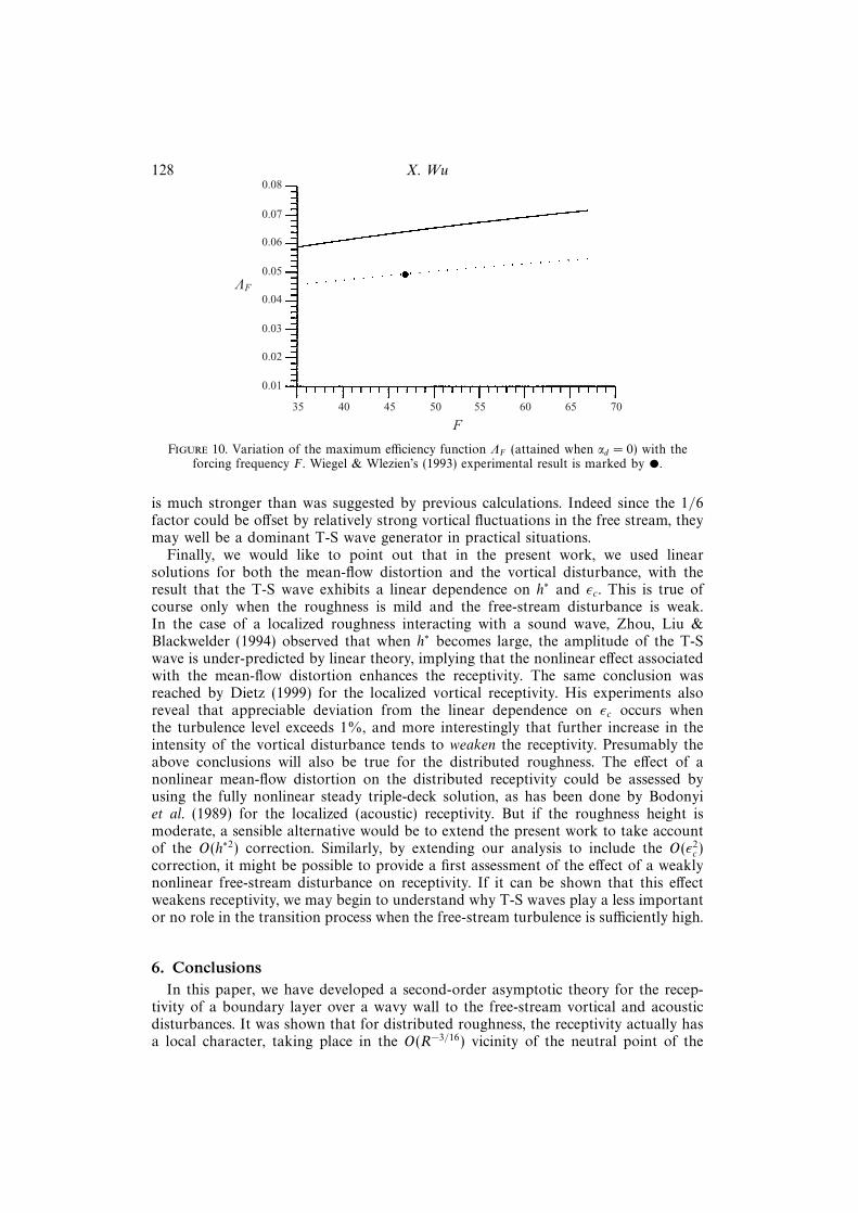
128 X. Wu

0.01

0.06

0.05

0.04

0.03

0.02

35

KF

0.07

0.08

40 45 50 55 60 65 70

F

Figure 10. Variation of the maximum efficiency function ΛF (attained when αd = 0) with theforcing frequency F . Wiegel & Wlezien’s (1993) experimental result is marked by •.

is much stronger than was suggested by previous calculations. Indeed since the 1/6factor could be offset by relatively strong vortical fluctuations in the free stream, theymay well be a dominant T-S wave generator in practical situations.

Finally, we would like to point out that in the present work, we used linearsolutions for both the mean-flow distortion and the vortical disturbance, with theresult that the T-S wave exhibits a linear dependence on h∗ and εc. This is true ofcourse only when the roughness is mild and the free-stream disturbance is weak.In the case of a localized roughness interacting with a sound wave, Zhou, Liu &Blackwelder (1994) observed that when h∗ becomes large, the amplitude of the T-Swave is under-predicted by linear theory, implying that the nonlinear effect associatedwith the mean-flow distortion enhances the receptivity. The same conclusion wasreached by Dietz (1999) for the localized vortical receptivity. His experiments alsoreveal that appreciable deviation from the linear dependence on εc occurs whenthe turbulence level exceeds 1%, and more interestingly that further increase in theintensity of the vortical disturbance tends to weaken the receptivity. Presumably theabove conclusions will also be true for the distributed roughness. The effect of anonlinear mean-flow distortion on the distributed receptivity could be assessed byusing the fully nonlinear steady triple-deck solution, as has been done by Bodonyiet al. (1989) for the localized (acoustic) receptivity. But if the roughness height ismoderate, a sensible alternative would be to extend the present work to take accountof the O(h∗2) correction. Similarly, by extending our analysis to include the O(ε2

c)correction, it might be possible to provide a first assessment of the effect of a weaklynonlinear free-stream disturbance on receptivity. If it can be shown that this effectweakens receptivity, we may begin to understand why T-S waves play a less importantor no role in the transition process when the free-stream turbulence is sufficiently high.

6. ConclusionsIn this paper, we have developed a second-order asymptotic theory for the recep-

tivity of a boundary layer over a wavy wall to the free-stream vortical and acousticdisturbances. It was shown that for distributed roughness, the receptivity actually hasa local character, taking place in the O(R−3/16) vicinity of the neutral point of the

Receptivity of boundary layers with distributed roughness 129

T-S wave. In this region, the forcing due to the interaction between the unsteadydisturbance and the mean-flow distortion is in resonance with the T-S wave, with theresult that the latter develops from the small-amplitude response upstream.

The high-Reynolds-number approach adopted in the present work allowed us tocalculate the amplitudes of the excited T-S waves in a systematic and self-consistentway. Moreover for the vortical receptivity, it overcame the difficulty of specifying theprofile of the disturbance in the free stream, by showing that the detailed profileis largely irrelevant. This made an appropriate comparison between the theory andexperiments possible for the first time. A good agreement has been observed. Ourresults also indicate that the boundary-layer receptivity to the free-stream turbulenceis much stronger than suggested by previous calculations.

The theoretical results for the acoustic receptivity have also been compared withthe relevant experiments. It is found that our first-order theory agrees very well withmeasurements, while the second-order theory over predicts. This discrepancy remainsto be resolved by further investigations.

The author would like to thank Professor J. T. Stuart, Professor M. Gaster andDr S. J. Cowley for helpful discussions. Dr M. E. Goldstein and the referees arethanked for their comments and suggestions, which have led to improvement of thepaper. The computations were carried out on a computer supported by EPSRC grantGR/L65666/01.

Appendix A. The O(ε2) correction to the dispersion of T-S wavesThe O(ε2) correction to the T-S wave dispersion can be obtained by seeking the

solutions to the quantities with the subscript ‘3’ in each deck and matching, aswas described in Smith (1979a) and § 3. The final outcome is the equation whichdetermines α3 and ω3:

aα3

α1

+ η0Ai(η0)

(λ0ω1

α1γ1

− 1

)ω3

ω1

=iλ0(iα1λ0)

2/3

γ21

[α2

γ1

+γ1(α2 − ω1)

α21

− γ21

α1

(J∞ − J0)

]×(

ω2

ω1

− 2

3

α2

α1

)η2

0Ai(η0)− 1

3

α2

α1

Ai′(η0)

+

(γ1I2 − ω1

α1

)(ω2

ω1

− 2

3

α2

α1

)η0Ai(η0)

+iλ0(iα1λ0)

2/3

α21

[α1γ1(I2J0 +H5 −H3)− ω1(H6 + J0 + 2I1 − I2) +

α21α2

γ21

I2

]Ai′(η0)

+iλ0(iα1λ0)

2/3

γ21

[−3(2α2

1 + β2)α22

2α1γ31

+(2α2 + ω1)α2

α1γ1

− 2γ1ω2

α21

− (ω21 − 2α2ω1)γ1

α31

]Ai′(η0)

− iλ0(iα1λ0)2/3

α1γ1

1

18

α22

α21

(η30Ai′(η0) + 3η2

0Ai(η0)− 2Ai′(η0))

+1

2

(ω2

ω1

− α2

α1

)(ω2

ω1

− 1

3

α2

α1

)η2

0(Ai(η0) + η0Ai′(η0))

−

1

18

α22

α21

(−η20Ai′(η0) + 2η0Ai(η0)) +

2

3

α2

α1

(ω2

ω1

− α2

α1

)η0Ai(η0)

−1

2

(ω2

ω1

− α2

α1

)(ω2

ω1

− 1

3

α2

α1

)η2

0Ai′(η0)

, (A 1)

130 X. Wu

where the constants I1, I2 etc. denote the values at x0 = 1 of the integrals defined asfollows

I1(x) =

∫ ∞0

(UB − 1) dy, (A 2)

I2(x) =

∫ ∞0

(U2B − 1) dy, (A 3)

J0(x) = −∫ a

0

(1

U2B

− 1

λ2y2

)dy +

1

λ2a, (A 4)

J∞(x) =

∫ ∞a

(1

U2B

− 1

)dy − a; (A 5)

H3 =

∫ a

0

U2B

∫ y

a

dy1

U2B

dy +

∫ ∞a

(1

U2B

− 1

)dy

∫ ∞a

(U2B − 1)dy − a

+

∫ ∞a

(U2B − 1)(y − a) dy −

∫ ∞a

U2B

∫ ∞y

(1

U2B

− 1

)dy1

dy + 1

2a2,

H5 =

∫ ∞0

(1

U2B

− 1

)∫ y

0

U2Bdy1

dy −

∫ ∞0

y(U2B − 1) dy,

H6 = 2

∫ ∞a

(1

U3B

− 1

)dy −

∫ ∞a

(1

U2B

− 1

)dy + 2

∫ a

0

(1

U3B

− 1

λ3y3

)dy − 1

λ3a2− a.

In all the expressions above, the parameter a is arbitrary provided a 6= 0. Since theBlasius profile UB is a function of the similarity variable y = y/x1/2, it is convenient,when evaluating these integral, to choose a = a0x

1/2 with a0 being independent ofx. It follows that I2, J0 and J∞ are all proportional to x1/2 so that their expansionsabout x0 are

I2(x) = I2(0) + ( 12I2(0)x1)R

−3/16 + · · · ,J0(x) = J0(0) + ( 1

2J0(0)x1)R

−3/16 + · · · ,J∞(x) = J∞(0) + ( 1

2J∞(0)x1)R

−3/16 + · · · .

(A 6)

Appendix B. The constants r0, r1, r2 and the function U (2)TS

r0 = 13iα−1

1 (iα1λ0)2/3(J∞ − J0)

(Ai′(η0) + 2η2

0Ai(η0))− 2

3λ−1

0 γ1η0Ai(η0)I2

+iω1(iα1λ0)−1

23η0Ai(η0)−

∫ ∞η0

Ai(η)dη − 2

3

(iα1λ0)5/3

α21γ1

[Ai′(η0)− η20Ai(η0)]

+ 2

3i(α1γ1)

−1(iα1λ0)2/3 (2α2

1 + β2)

γ21

α2

α1

(Ai′(η0)− η20Ai(η0))

+i(α1γ1)−1(iα1λ0)

2/3

2

9

α2

α1

(η3

0Ai′(η0) + Ai′(η0))

+2

3

(ω2

ω1

− α2

α1

)η2

0(η0Ai′(η0) + Ai(η0))

− 23λ−1

0

(ω2

ω1

− 5α2

3α1

)η0Ai(η0) +

(ω2

ω1

− 2α2

3α1

)η2

0Ai′(η0)

. (B 1)

Receptivity of boundary layers with distributed roughness 131

r1 =i(2α2

1 + β2)

α1γ31

(iα1λ0)2/3

(ω2

ω1

− 2

3

α2

α1

)η2

0Ai(η0) +2

3

α2

α1

Ai′(η0)

+

iω1(3α21 + 2β2)

α21γ

31

(iα1λ0)2/3Ai′(η0)− iα2(iα1λ0)

2/3

2β2

α21γ

31

+3(2α2

1 + β2)

γ51

Ai′(η0)

−λ−10 α2

1γ−11 I2

∫ ∞η0

Ai(η) dη. (B 2)

r2 = −λ−10

ω2

ω1

η0Ai(η0) +2

3

(iα1λ0)5/3

α21γ1

[Ai′(η0)− η20Ai(η0)]− 2γ1I2

∫ ∞η0

Ai(η) dη

.

(B 3)

U(2)TS =

[1− ε

(α2

α1

− q∞)]∫ η

η0

Ai(η) dη − β21

γ21

Ai′(η0) L(η)

+ε

(ω2

ω1

− α2

α1

)η0(Ai(η)−Ai(η0)) +

1

3

α2

α1

(ηAi(η)− η0Ai(η0))

−εβ2

γ21

[(

ω2

ω1

− 2

3

α2

α1

)η2

0Ai(η0)− 2α1α2

γ21

Ai′(η0)

] L(η)

+

(ω2

ω1

− α2

α1

)η0Ai′(η0) L′(η) +

1

3

α2

α1

Ai′(η0)η L′(η)

+

∫ ∞η0

Ai(η) dη

Ai2(η0)

(ω2

ω1

− 2

3

α2

α1

)η0Ai′(η0)Ai(η)

. (B 4)

Appendix C. Matching between the T-S wave solution and the upstreamforced response

To demonstrate more clearly that the T-S wave grows out of the forced responsein the pre-resonance region, we now show that these two solutions match in theasymptotic sense. The vortical case will be used for the purpose of illustration. At anarbitrary location in the pre-resonance region, x say, the forced response in the lowerdeck has expansions similar to (3.62)–(3.65) provided that the T-S wave is excludedand the mean-flow deviation suppressed. Then V4 and V5 would satisfy (3.98) and(3.104), and their solutions can be written as (3.99) and (3.105) respectively, providedof course that A and q2 are set to zero, and λ0 is replaced by λ. The solutions in theupper and main decks are similar to those given in § 3.1 and § 3.3. Then on applyingthe boundary and matching conditions, we find that q4 and q5 are determined by

q4 =λFv

∆(λ)eiαdx1 , (C 1)

q5 =

(ω1

α1

− γ1I2(x) +

(1 +

α21

γ21

)α2

α1

)− ∆1(λ)

∆(λ)

q4 +

λFc

∆(λ)eiαdx1 , (C 2)

where ∆(λ) and ∆1(λ) are defined by (3.75) and (3.87) respectively with λ0 beingunderstood as λ, the dependence on which is through η0, I2, J0 and J∞. A Taylor

132 X. Wu

expansion of ∆(λ) about λ0 shows that as x→ x0,

q4 → λ20Fv

iα1b(λ− λ0)= R3/16(N/σ)(−x1)

−1 eiαdx1 , (C 3)

indicating that q4 matches to A; see (3.113). Similarly, expanding ∆1(λ), and I2, J∞and using the relations that

∆1(λ0) = 0,∂I2

∂λ(λ0) = −I2(0)/λ0,

∂J0

∂λ(λ0) = −J0(0)/λ0,

∂J∞∂λ

(λ0) = −J∞(0)/λ0,

we find that

q5 →

ω1

α1

− γ1I2(0) +

(1 +

α21

γ21

)α2

α1

− λ0∆′1(λ0)

iα1b

N

σ− λ2

0Fc

iα1λ1b

R3/16(−x1)

−1 eiαdx1 .

(C 4)A comparison with (3.115) suggests that q5 matches to q2 if

ω1

α1

− γ1I2(0) +

(1 +

α21

γ21

)α2

α1

b− λ0∆

′1(λ0)

iα1

= λ0(r0 + r2). (C 5)

The above identity is verified by a direct calculation using (3.87).

REFERENCES

Bodonyi, R. J., Welch, W. J. C., Duck, P. W. & Tadjfar, M. 1989 A numerical study of theinteraction between unsteady free-stream disturbances and localized variations in surfacegeometry. J. Fluid Mech. 209, 285–308.

Brown, S. N. & Stewartson, K. 1973 On the propagation of disturbances in a laminar boundarylayer. Math. Proc. Camb. Phil. Soc. 73, 493–514.

Choudhari, M. 1993 Boundary-layer receptivity due to distributed surface imperfections of adeterministic or random nature. Theor. Comput. Fluid Dyn. 4(3), 101–117.

Choudhari, M. 1994 Distributed acoustic receptivity in laminar flow control configurations. Phys.Fluids 6, 489–506.

Choudhari, M. 1996 Boundary-layer receptivity to three-dimensional unsteady vortical disturbancesin free stream. AIAA Paper 96-0181.

Choudhari, M. & Streett, C. L. 1992 A finite Reynolds number approach for the prediction ofboundary-layer receptivity in localized regions. Phys. Fluids 4, 2495–2514.

Crouch, J. D. 1992a Localized receptivity of boundary layers. Phys. Fluids 4, 1408–1414.

Crouch, J. D. 1992b Non-localized receptivity of boundary layers. J. Fluid Mech. 244, 567–581.

Crouch, J. D. 1994 Distributed excitation of Tollmien–Schlichting waves by vortical free-streamdisturbances. Phys. Fluids 6, 217–223.

Dietz, A. J. 1996 Distributed boundary layer receptivity to convected vorticity. AIAA Paper 96-2083.

Dietz, A. J. 1998 Boundary-layer receptivity to transient convected disturbances. AIAA J. 36,1171–1177.

Dietz, A. J. 1999 Local boundary-layer receptivity to a convected free-stream disturbance. J. FluidMech. 378, 291–317.

Duck, P. W., Ruban, A. I. & Zhikharev, C. N. 1996 Generation of Tollmien–Schlichting waves byfree-stream turbulence. J. Fluid. Mech. 312, 341–371.

Goldstein, M. E. 1983 The evolution of Tollmien–Schlichting waves near a leading edge. J. FluidMech. 127, 59–81.

Goldstein, M. E. 1985 Scattering of acoustic waves into Tollmien–Schlichting waves by smallstreamwise variations in surface geometry. J. Fluid Mech. 154, 509–529.

Goldstein, M. E. & Hultgren, L. S. 1987 A note on the generation of Tollmien–Schlichting wavesby sudden surface-curvature change. J. Fluid. Mech. 181, 519–525.

Gulyaev, A. N., Kozlov, V. E., Kuznetson, V. R., Mineev, B. I. & Sekundov, A. N. 1989Interaction of laminar boundary layer with external turbulence. Izv. Akad. Nauk SSSR Mekh.Zhid. Gaza 6, 700–710.

Receptivity of boundary layers with distributed roughness 133

Hall, P. & Smith, F. T. 1984 On the effects of non-parallelism, three-dimensionality and modeinteraction in nonlinear boundary-layer stability. Stud. Appl. Maths 71, 91–120.

Kendall, J. M. 1985 Experimental study of disturbances produced in pre-transitional laminarboundary layer by weak free stream turbulence. AIAA Paper 85-1695.

Kendall, J. M. 1990 Boundary-layer receptivity to free-stream turbulence. AIAA Paper 90-1504.

Kerschen, E. J. 1991 Linear and nonlinear receptivity to vortical free-stream disturbances. InBoundary Layer Stability and Turbulence (ed. D. C. Reda, H. L. Reed & R. K. Kobayashi)ASME FED, vol. 114, pp. 43–48.

Kovasznay, L. S. G. 1953 Turbulence in supersonic flow. J. Aero. Sci. 20, 657–682.

Leib, S. J., Wundrow, D. W. & Goldstein, M. E. 1999 Effect of free-stream turbulence and othervortical disturbances on a laminar boundary layer. J. Fluid Mech. 380, 169–203.

Lin, C. C. 1946 On the stability of two-dimensional parallel flows. Part 3. Stability in a viscousfluid. Q. Appl. Maths. 3, 277–301.

Morkovin, M. V. 1969 Critical evaluation of transition from laminar to turbulent shear layerswith emphasis on hypersonically travelling bodies. AFFDL-TR 68-149. US Air Force FlightDynamics Laboratory, Wright Patterson Air Force Base, Ohio.

Reshotko, E. 1976 Boundary layer stability and transition. Ann. Rev. Fluid Mech. 8, 311–349.

Ruban, A. I. 1983 Nonlinear equation for the amplitude of Tollmien–Schlichting waves in theboundary layer. Izv. Akad. Nauk. SSSR Mekh. Zhid. Gaza 6, 60–67.

Ruban, A. I. 1984 On Tollmien–Schlichting wave generation by sound. Izv. Akad. Nauk. SSSR Mekh.Zhid. Gaza 5, 44 (in Russian; English Translation: Fluid Dyn. 19, 709–716 (1985)).

Ruban, A. I., Duck, P. W. & Zhikharev, C. N. 1996 The generation of Tollmien–Schlichting wavesby freestream vortical perturbations. AIAA Paper 96-2123.

Ryzhov, O. S. & Terent’Ev, E. D. 1977 On unsteady boundary layer with self-induced pressure.Prikl. Mat. Makh. 41(6), 277–301.

Smith, F. T. 1979a On the nonparallel flow stability of the Blasius boundary layer. Proc. R. Soc.Lond. A 366, 91–109.

Smith, F. T. 1979b Nonlinear stability of boundary layers for disturbances of various sizes. Proc. R.Soc. Lond. A 368, 573–589.

Tam, C. K. W. 1981 The excitation of Tollmien–Schlichting waves in lower subsonic boundary layersby free-stream sound waves. J. Fluid Mech. 109, 483–501.

Terent’ev, E. D 1981 The linear problem of a vibrator in a subsonic boundary layer. Prikl. Math.Mech. 45, 1049–1055.

Wiegel, M. & Wlezien, R. W. 1993 Acoustic receptivity of laminar boundary layers over wavywalls. AIAA Paper 93-3280.

Wu, X. 1999 Generation of Tollmien–Schlichting waves by convecting gusts interacting with sound.J. Fluid Mech. 397, 285–316.

Zhigulev, V. N. & Tumin, A. M. 1987 Origin of Turbulence. NAUKA, Novosibirsk.

Zhou, M. D., Liu, D. P. & Blackwelder, R. F. 1994 An experimental study of receptivity ofacoustic waves in laminar boundary layers. Exps. Fluids 17, 1–9.