科研費シンポジウム

"Recent Progress in Spatial and/or Spatio-

temporal Data Analysis"

Keynote speaker: Prof. Daniel A. Griffith

(Univ. of Texas at Dallas)

開催日：2020 年 10 月 30 日

オンライン開催

科研費シンポジウム

"Recent Progress in Spatial and/or Spatio-temporal Data Analysis"

開催責任者：松田安昌(東北大学)

文部科学省科学研究費補助金　基盤研究(A)20H00576　　　　　　　　　　「大規模複雑データの理論と方法論の革新的展開」 　　　　　　　　　　研究代表者：青嶋誠（筑波大学）

内容・目的

Spatial and/or space- time problems in a wide range of areas have attracted more and more attention especially after 2000, with a proliferation of books, conferences, and papers. The explosion of interests in spatial statistics has been largely fueled by the increased availability of large spatial and spatio-temporal datasets across many fields, such as from the recent progress of geographic information systems (GIS). Spatial statistics can be regarded as one of the most critical areas in statistics to work for many modern issues in the age of big data. This conference welcomes presentations in the broad areas aiming to develop spatial and/or spatio-temporal analysis.

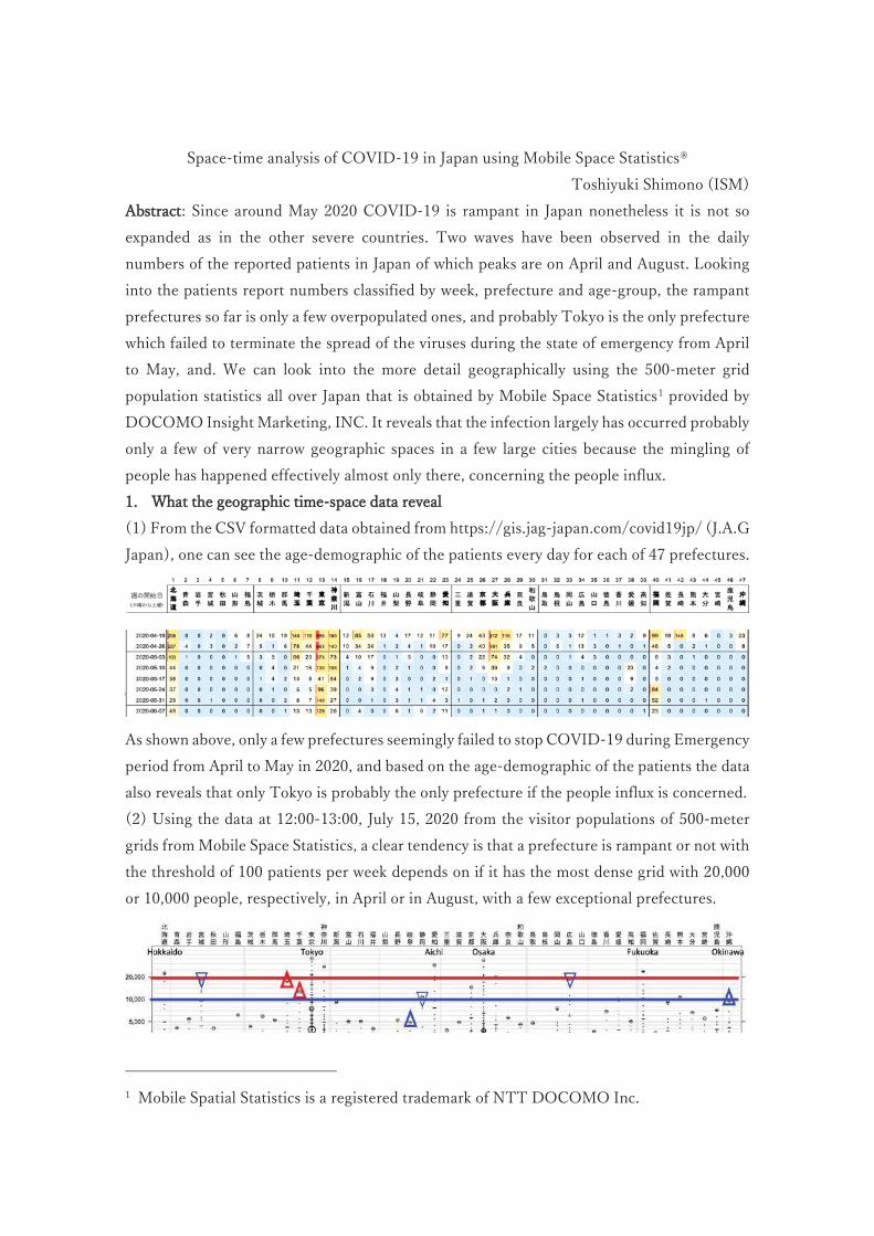
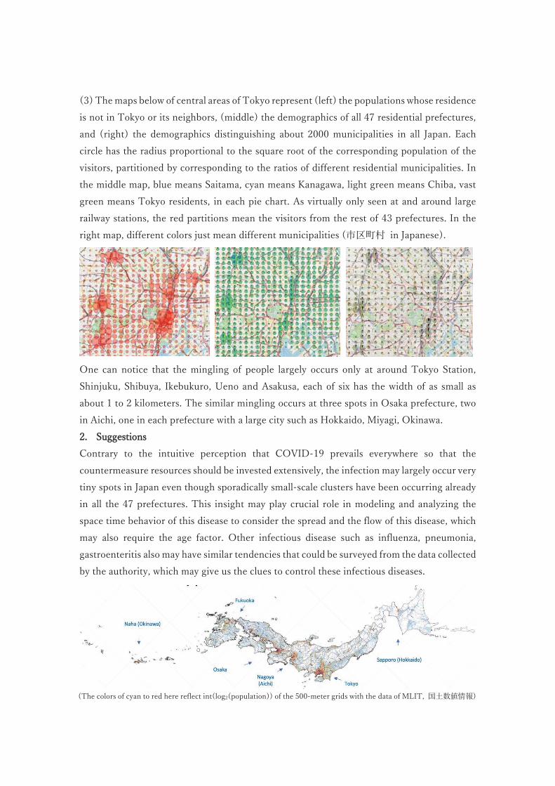
Program Friday, Oct 30, 2020 10:00-11:00 Griffith, D. (Univ. Texas at Dallas) Important considerations about space-time data: modeling, scrutiny and ratification 11:00-11:30 Murakami, D. (ISM) Compositionally-warped additive mixed modeling for large non-Gaussian data: Application to COVID-19 analysis 11:30-12:00 Shimono, T. (ISM) Space-time analysis of COVID-19 in Japan using mobile space statistics(R). Lunch break 13:30-14:00 Yajima, Y. (Tohoku U.) On estimation of intrinsically stationary random fields. 14:00-14:30 Sugasawa, S. (Univ. Tokyo) Spatially clustered regression 14:30-15:00 Toda,H. (Nagoya Institute of Technology) Post-selection Inference for spatio-temporal trajectory segmentation break 15:15-15:45 Hirano, T. (Kanto Gakuin U,) A multi-resolution approximation via linear projection for large spatial datasets 15:45-16:15 Matsui, M. (Nanzan U.) Testing independence of continuous time stochastic processes -- toward independence test for random fields -- 16:15-16:45 Matsuda, Y. (Tohoku U.) Space time ARMA model

1

ABRIDGED VERSION1—IMPORTANT CONSIDERATIONS ABOUT SPACE-TIME DATA: MODELING, SCRUTINY, AND RATIFICATION

Daniel A. GriffithAshbel Smith Professor of Geospatial Information Sciences, U. of Texas at Dallas

1. IntroductionSpace-time data analysis has a literature spanning many decades, including Cliff et al. (1975), Bennett (1979), Heuvelink and Griffith (2010), and Cressie and Wikle (2011), among others. This literature’smost modern section includes matrix models and Markov chain analysis, dynamic geographic optimi-zation, and numerous statistical entries by Gelfand and his colleagues, and Christakos and his col-leagues, inter alia. This paper acknowledges, without reviewing, this literature; instead, it focuses onthe evolution of the space-time autocorrelation concept, a vital property of space-time data.

Autocorrelation (i.e., correlation amongst a single variable’s observations) characterizes some correlated data family members, including time series, space series, and space-time series (Griffith, 2020). Its all-inclusive literature covers nearly two centuries, beginning with temporal autocorrela-tion—correlation among a single variable’s data values at consecutive points in time—followed byspatial autocorrelation (SA)—correlation among a single variable’s data values at pairs of neighboring points in space—and culminating in space-time autocorrelation—correlation among a single varia-ble’s data values at two consecutive points in time as well as nearby points in space.

Although interest in space-time data dates back at least to the mid-1900s, almost exclusively withseparate treatments of space and time, such socio-economic and demographic datasets remained scarce until the 2000s. Unfortunately, earlier widely embraced accessible datasets furnished by An-drews and Herzberg (1985), for example, are fraught with entry errors that almost certainly scramble their space and/or time orderings, highlighting that accuracy is a fundamental space-time data quality assessment requirement, one complicated by the relatively large size and complexity of many space-time datasets vis-à-vis solely their time series or space series components.

The purpose of this paper is to address two important issues. The first is space-time autocorrela-tion in terms of its individual temporal and SA constituents latent in, and accuracy assessment prelim-inaries for evaluating the veracity of, a space-time dataset. The second is furnishing insights, articulat-ing autocorrelation relationships, and raising awareness about probable best practices when undertak-ing an analysis of space-time data. Exemplifications of discussions employ annual United States (US) county population data for 1969-2019, the overwhelming majority of which the policy setting US Na-tional Cancer Institute (NCI) Surveillance, Epidemiology, and End Results (SEER) Program uses. The data generating process here is a combination of the US decennial census survey and annual updates to these census figures extracted from official government records that add births, subtract deaths, and adjust for net migration as well as age cohort shifts attributable to the passing of time.

2. The data: a brief overviewThe US NCI SEER dataset currently consists of annual county time series from 1969 to 2018. This is an appealing dataset because it satisfies expert opinion asserting that the simplest of analyses requires a time series with a minimum of about 50 observations (see Hanke and Wichern, 2013). The selectedgeographic sample of these data for evaluation here contains the following six states: Ohio (OH), Ore-gon (OR), Florida (FL), Maine (ME), South Dakota (SD), and Texas (TX).

3. Temporal, spatial, and space-time autocorrelationOn average, temporal autocorrelation ( T) tends to be stronger than SA ( s), frequently exceeding0.95; the degree of SA for socio-economic and demographic data tends to be in the 0.4 to 0.6 range,with most remotely sensed s value in excess of 0.9. These two descriptions underscore the empirical tendency for both forms of autocorrelation to be positive, with negative SA being much rarer than negative temporal autocorrelation. An intermingling of these two kinds of autocorrelation in space-time data routinely results in temporal autocorrelation dominating SA.

Each of the sample states has n counties (16 < n < 254), with each of these counties having a time series of length 51 before differencing, and 50 after differencing. Autocorrelation in each of the differ-enced time series is well-described by a lag-one model specification; however, temporal autocorrela-

1This is an abridged version of a paper with the same title that presently is under review by Transactions in GIS.

2

tion is not very concentrated for most of the individual states. Although the preponderance of time se-ries display relatively high degrees of positive temporal autocorrelation, the considerable heterogene-ity of parameter estimates here fails to support the parsimonious positing of a single temporal autocor-relation parameter in a space-time autocorrelation specification, even separately state-by-state.

Each of the states has 50 time-differenced log-population density (improving normality) geo-graphic distributions. Simultaneous autoregressive (i.e., SAR) spatial regression model estimation re-sults reveal that a rook adjacency definition coupled with a second-order model specification de-scribes autocorrelation in each of the space series well, and that individual state SA also is not very concentrated. The considerable heterogeneity of parameter estimates here once more fails to support the parsimonious positing of a single SA parameter in a space-time autocorrelation specification.

The preceding discussion treats temporal and SA separately, when they actually coalesce in space-time situations. The conceptualization and description of this interacting combination tends to occur in three different ways. Cliff et al. (1975) furnish one of the first comprehensive treatments of this conceptualization, presenting a space-time autoregressive (STAR) model specification of the fol-lowing two forms: space-time lag (i.e., SA arises in terms of the preceding time period), and contem-poraneous (i.e., SA is instantaneous, arising from the current time period). Meanwhile, contemporary statistical mixed models theory (e.g., West et al., 2007) furnishes a third form by positing a random effects (RE) specification to describe space-time data. This RE conceptualization maintains that re-gression model residuals are the sum of a systematic component, arising from, say, missing variables, plus a stochastic component, arising from the independent and identically distributed (iid) regression errors assumption. A standard chorological regression analysis requires additional information to sep-arate these two components. One ancillary information source is repeated measures, such as time se-ries of annual population densities, and another is a spatial weights matrix (SWM) that allows the par-titioning of the systematic part into two sub-parts, a spatially structured RE (SSRE), which relates to a SWM, and a spatially unstructured RE (SURE), which is geographically random in nature, and hence void of SA. This RE term is a time invariant map that repeats itself for each point in a time series; it isa common factor across time instilling temporal autocorrelation into a space-time series dataset.

4. Space-time data accuracy assessmentOne goal traversing the exploratory diagnostic computation of n temporal autocorrelation estimates,

, and T SA estimates, , is assessing whether or not their respective variations are within margins of design-based or model-based stochastic sampling error. Sufficiently narrow estimate ranges sup-port a parsimonious space-time data description whose predictive power reinforcements sustains the fidelity of its implications. Another useful investigative task is to inspect the global mean and varia-tion of a space-time dataset. Yet a third helpful examination ascertains the degree to which space-time dataset parts may be interpolation and extrapolation technique constructions. Inspecting data extremes as well as variance homogeneity are two additional interrelated standard considerations. A further ap-praisal concerns model overfitting and the quality of any recognized imputed values. These seven as-sessments constitute best practice procedures for initiating a data scrutiny and ratification plan.

5. ConclusionsThis paper establishes seven beneficial best practices enabling a space-time analyst to become more familiar with a given dataset, to more easily address data debugging and remediation issues, and tobetter express the soundness of inferred generalizations coupled with more robust finding limitations.

6. ReferencesAndrews, D., and A. Herzberg. 1985. Data: A Collection of Problems from Many Fields for the Student and Re-

search Worker. New York: Springer-Verlag.Cliff, A., P. Haggett, J. Ord, K. Bassett, and R. Davies. 1975. Elements of Spatial Structure: A Quantitative Ap-

proach. London: Cambridge U. Press.Cressie, N., and C. Wikle. 2-11. Statistics for Spatio-Temporal Data. New York: Wiley.Griffith, D. 2020. A family of correlated observations: From independent to strongly interrelated ones, Stats, 3:

166-184; doi:10.3390/stats3030014Hanke, J., and D. Wichern. 2013. Business Forecasting (9th ed.). Upper Saddle River, NJ: Pearson.Heuvelink, G., and D. Griffith. 2010. Space–time geostatistics for geography: A case study of radiation monitor-

ing across parts of Germany, Geographic Analysis, 42: 161-170.West, B., K. Welch, and A. Galecki. 2007. Linear Mixed Models: A Practical Guide Using Statistical Software.

New York: Chapman & Hall/CRC.

Compositionally-warped additive mixed modeling for large non-Gaussian data: Application to COVID-19 analysis

Daisuke Murakami

Institute of Statistical Mathematics, 10-3 Midoricho, Tachikawa, Tokyo, 190-8562, Japan

Email: dmuraka@ism.ac.jp

1. Outline

An increasing number of non-Gaussian geospatial data is becoming available. At the same time,

the size of spatial data rapidly grows together with the development of sensing technology. Given these

backgrounds, this study develops a flexible additive mixed modeling approach for large non-Gaussian

data. The development is done by combining an additive mixed model (AMM), which accommodates

spatial and other effects, with the compositionally-warped Gaussian process (CWGP; Rois and Tober,

2019) estimating the shape of data distribution that can be either Gaussian or non-Gaussian possibly

have skewness, fat tail, and other properties. The proposed model, termed compositionally-warped

additive mixed model (CAMM) is estimated through a restricted likelihood maximization balancing

model accuracy and complexity. Monte Carlo experiments shows that the proposed approach accurately

model a wide variety of non-Gaussian data accuracy without losing computational efficiency relative

to the linear AMM. The developed CAMM is applied to a spatiotemporal analysis of COVID-19 in

Japan. The developed approach will be implemented in an R package spmoran.

2. Compositionally-warped additive mixed model (CAMM)

The proposed model describes non-Gaussian explained variables | ∈ {1, … , } as follows:

( ) = , + ( , ) + , … . . ~ (0, ). (1)

( , ) is a smooth function depending on l-th covariate , , accommodating a wide variety of effects.

Just like the classical AMM, this term can capture linear/non-linear effects, spatial and/or temporal

effects, and other effects. (∙) is a function transforming the non-Gaussian variable to a nearly Gaussian variable.

Interestingly, a wide variety of non-Gaussian variables can be transformed to Gaussian variables

without assuming data distribution if the (∙) function is defined by concatenating D transformation

functions as below (see Rois and Tober, 2019): ( ) = (⋯ ( )) , (2)

where ∈ { , , … , }. The d-th transformation function ( ) in Eq. (2) is specified as ( ) = + sinh ( arcsinh( ) − ), (3)

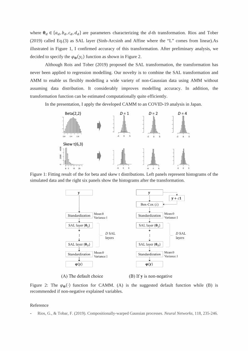
where ∈ { , , , } are parameters characterizing the d-th transformation. Rios and Tober

(2019) called Eq.(3) as SAL layer (Sinh-Arcsinh and Affine where the “L” comes from linear).As

illustrated in Figure 1, I confirmed accuracy of this transformation. After preliminary analysis, we

decided to specify the ( ) function as shown in Figure 2.

Although Rois and Tober (2019) proposed the SAL transformation, the transformation has

never been applied to regression modelling. Our novelty is to combine the SAL transformation and

AMM to enable us flexibly modelling a wide variety of non-Gaussian data using AMM without

assuming data distribution. It considerably improves modelling accuracy. In addition, the

transformation function can be estimated computationally quite efficiently.

In the presentation, I apply the developed CAMM to an COVID-19 analysis in Japan.

Figure 1: Fitting result of the for beta and skew t distributions. Left panels represent histograms of the simulated data and the right six panels show the histograms after the transformation.

Figure 2: The (∙) function for CAMM. (A) is the suggested default function while (B) is recommended if non-negative explained variables.

Reference

- Rios, G., & Tobar, F. (2019). Compositionally-warped Gaussian processes. Neural Networks, 118, 235-246.

On Gaussian semiparametric estimation fortwo-dimensional intrinsic stationary random fields

Yoshihiro YajimaTohoku University

2020. Oct 30.

Abstract

We propose two estimators of two-dimensional intrinsic stationary random fields (ISRFs) observed on aregular grid and derive their asymptotic properties. Originally they are proposed to estimate prametersof long memory models of stationary and nonstationary time series. One is the log-periodgram regressionestimator (Robinson(1995a); Velasco(1995a)) and the other is the Gaussian semiparametric estimtor(the localWhittle estimator Robinson(1995b); Velasco(1999b)). We apply them to two dimensional ISRFs. TheseISRFs include a fractional Brownian field, which is a Gaussian random field and is used to model manyphysical processes in space(Mandelbrot, B.B. and Van Ness, J.W. (1968)). The estimators are consistent andhave the limiting normal distributions as the sample size goes to infinity. We also list some problems suchas testing isotropy or applications to more general models that are to be solved in future.

Keywords:intrinsic stationary random fields; spatio-temporal models; local Whittle estimator; log peri-odogram regression; fractional Brownian field.

References

Mandelbrot, B.B. and Van Ness, J.W. (1968). Fractional Brownian motion, fractal noises and applications.SIAM. Rev. 10 422-437.

Robinson,P.M. (1995a). Log periodogram regression of time series with long range dependence. Ann. Statist.23 1048-1072.

Robinson,P.M. (1995b). Gaussian semiparametric estimation of long range dependence. Ann. Statist. 231630-1661.

Velasco,C. (1999a). Non-stationary log-periodogram regression. J. Econometrics 91 325-371.

Velasco,C. (1999). Gaussian semiparametric estimation of non-stationary time series. J. Time Ser. Anal.20 87-127.

1

Spatially Clustered Regression

Shonosuke Sugasawa

Center for Spatial Information Science, The University of Tokyo

1 Introduction

Geographically weighted regression (GWR) is widely adopted for modeling possibly

spatially varying regression coefficients. However, GWR is known to be numerically

unstable and may produce extreme estimates of coefficients especially when covari-

ates are spatially correlated. Recently, Li and Sang (2019) adopted fused lasso to

shrink regression coefficients in neighboring locations, but it can be computationally

intensive under large spatial data. In this work, we propose a new strategy for spatial

regression that takes account of spatial heterogeneity in regression coefficients. The

proposed method can be easily estimated via a simple iterative algorithm, and it can

handle variable selection or semiparametric modeling.

2 Spatially Clustered Regression

Let yi be a response variable and xi is a vector of covariates in the ith location, for

i = 1, . . . , n, where n is the number of samples. We suppose we are interested in the

conditional distribution f(yi|xi; θi), where θi is a vector of unknown parameters. Here

θi may change over different locations and represent spatial heterogeneity. For exam-

ple, f(yi|xi; θi) = φ(yi;xti1θi + xti2γ, σ

2i ). We assume that geographical information si

(e.g. longitude and latitude) is also available for the ith location. We further assume

that n locations are divided into G groups and locations in the same group share

the same parameter values of θi. We introduce gi ∈ {1, . . . , G}, an unknown group

membership variable for the ith location, and let θi = θgi . Then, the distinct values

of θi’s reduce to θ1, . . . , θG, where θ = (θt1, . . . , θtG)

t is the set of unknown parameters.

1

Therefore, the unknown parameters in the model is the structural parameter θ and

membership parameter g = (g1, . . . , gn). Regarding the membership parameter, it

would be reasonable to consider that the membership in neighboring locations are

likely to have the same memberships, which means that the fitted conditional distri-

butions are likely to be the same in the neighboring locations. In order to encourage

such structure, we propose the following penalized likelihood:

Q(θ, g) ≡n∑

i=1

log f(yi|xi; θgi) + φ∑i<j

wijI(gi = gj), (1)

where wij = w(si, sj) ∈ [0, 1], w(·, ·) is a weighting function, and φ controls strength

of spatial similarity. The penalty function is motivated from the Potts model (Potts,

1952) and a similar penalty function is adopted in Sugasawa (2020). We define

the estimator of θ and g as the maximizer of the objective function Q(θ, g). The

maximization can be easily carried out by a simple iterative algorithm similar to

k-means algorithm. Owing to the simple formulation (1), the proposed strategy

allows several important extensions. For example, variable selection can be done

by introducing additional penalty function for θ, and semiparametric form for the

regression term can also be adopted.

We will report the numerical performance of the proposed method compared with

existing methods such as GWR or method by Li and Sang (2019) through simulation

studies and real data applications.

References

Li, F. and H. Sang (2019). Spatial homogeneity pursuit of regression coefficients for

large datasets,. Journal of the American Statistical Association 114, 1050–1062.

Potts, R. B. (1952). Some generalized order-disorder transformations. Mathematical

Proceedings of the Cambridge Philosophical Society 48, 106–109.

Sugasawa, S. (2020). Grouped heterogeneous mixture modeling for clustered data.

Journal of the American Statistical Association, to appear.

2

Post-selection Inference forSpatio-temporal Trajectory Segmentation

Hiroki Toda1, Yu Inatsu2, and Ichiro Takeuchi1, 2

1Nagoya Institute of Technology, 2Riken AIP

1 IntroductionTrajectory segmentation is a common task in spatio-temporal trajectory data analysis. It splitsa sequence of locations with time stamps into a small number of sub-sequences or segments withrespect to some criteria. Despite the development of a wide variety of methods [1], to date,little attention has been paid to quantifying the uncertainty of segment breakpoints identified bytrajectory segmentation. In this study, we aim to develop inference tools that provide valid p-valuesfor each breakpoint. The difficulty lies in the fact that the location of each breakpoint is selected bya segmentation algorithm, and this fact must be properly incorporated in the statistical inference.Unfortunately, if one uses classical statistical inference, the p-values or confidence intervals arenot valid anymore in the sense that the false positive rate cannot be controlled at the desiredsignificance level. To address this problem, we adopt the framework of Selective Inference (SI) [2](also known as Post-selection Inference), a new statistical inference framework for data-drivenhypotheses. This enables us to perform exact (non-asymptotic) inference conditioning on theselection procedure. Additionally, we introduce a parametric programing approach [3, 4] to solvethe problem that SI has low statistical power due to over-conditioning, which was assumed to beone of the major drawbacks of SI. To the best of our knowledge, this study is the first applicationof SI to trajectory data analysis. In the talk, we will demonstrate the performance of the proposedmethods when in animal trajectory data analysis.

2 Trajectory Segmentation and Statistical TestsLet T = [p1, p2, . . . , pn] denote a trajectory of length n, where each point pi = (xi, yi, ti) consistsof (x, y) location (and possibly additional parameters) of a moving object at time ti. A trajectorysegmentation algorithm splits the trajectory T into segments at breakpoints τ = (τ1, . . . , τK) withknown or unknown number of breakpoints K. Trajectory segmentation is mainly classified into twotypes, time series-based and topology-based algorithm. The former first converts the trajectoryinto univariate sequence xobs ∈ R

N of a feature (e.g., speed, acceleration and direction), thenchange-point detection is applied to xobs. The latter directly uses the locational data xobs =(x1, . . . , xn, y1, . . . , yn)� ∈ R

N as an input. We assume that xobs is a single observation drawnfrom X ∼ N(μ, Σ) ∈ R

N .We develop inference tools for the two types of algorithms. For time series-based algorithm, we

consider optimal change-point detection for a sequence with piecewise constant and piecewise linearmean. In the case of the piecewise constant, statistical test of interest might be H

(k)0 : μk = μk+1

v.s. H(k)1 : μk �= μk+1 for k ∈ {1, . . . , K}, where μk is the population mean of kth segment.

For topology-based algorithm, we consider Ramer-Douglas-Peucker (RDP) algorithm, which istraditional but popular because of its simplicity. Due to space limitations, we omit the details ofthe algorithms and statistical tests for each algorithm.

1

3 Selective InferenceThe basic idea of SI [2] is to make inference conditional on the selection event, which allows us toderive the exact (non-asymptotic) sampling distribution of a test statistic. Given a statistical testH0 and H1, we assume that the test statistic can be written in the form of η�xobs using somecontrast vector η ∈ R

N . Then, we have the following (two-sided) selective p-value:

p := PrH0

(|η�X| ≥ |η�xobs| | M(X) = M(xobs), A(X) = A(xobs), P⊥η X = P⊥

η xobs)

.

Note that p satisfies PrH0(p < α) = α, ∀α ∈ [0, 1]. The first condition M(X) = M(xobs) = τindicates the event that breakpoints τ are selected. The second condition A(X) = A(xobs)indicates the algorithm-dependent nuisance selection event that we had no choice but to conditionon for tractability in most cases. The condition P⊥

η X = P⊥η xobs is introduced for technical

reasons, where P⊥η = IN − cη� is the orthogonal projection matrix with c = Ση(η�Ση)−1.

Conditioning not only on the selection of breakpoints but also on the algorithm procedure itselfA(X) = A(xobs) makes the conditioning space smaller:

{X : M(X) = M(xobs), A(X) = A(xobs)} ⊆ {X : M(X) = M(xobs)}.

This leads low statistical power of SI. Existing exact SI framework has suffered from this over-conditioning problem.

Recently, we have developed a new SI framework [3, 4] that uses a parametric programmingtechnique to circumvent the over-conditioning. We define the parameterized data x′

obs(z) = cz +P⊥

η xobs with a parameter z ∈ R, then we have a valid selective p-value

p := PrH0

(|η�X| ≥ |η�xobs| | M(X) = M(xobs), P⊥η X = P⊥

η xobs)

= PrH0

(|z| ≥ |η�xobs| | M(x′obs(z)) = M(xobs)

).

By using this, we are able to perform powerful testing. We also have developed the effectiveprocedure to identify the all intervals of z where the same breakpoints τ are obtained, by searchingz over (−∞, ∞).

AcknowledgmentsThis work was supported by MEXT KAKENHI to I.T. (20H00601, 16H06538) and Y.I. (20H00601);from JST CREST awarded to I.T. (JPMJCR1502); and from RIKEN Center for Advanced Intel-ligence Project awarded to I.T.

References[1] Hendrik Edelhoff, Johannes Signer, and Niko Balkenhol. Path segmentation for beginners: An

overview of current methods for detecting changes in animal movement patterns. MovementEcology, 4, 12 2016.

[2] Jason D. Lee, Dennis L. Sun, Yuekai Sun, and Jonathan E. Taylor. Exact post-selectioninference, with application to the lasso. The Annals of Statistics, 44(3):907–927, Jun 2016.

[3] Vo Nguyen Le Duy, Hiroki Toda, Ryota Sugiyama, and Ichiro Takeuchi. Computingvalid p-value for optimal changepoint by selective inference using dynamic programming.arXiv:2002.09132, 2020. (to appear in NeurIPS 2020).

[4] Vo Nguyen Le Duy and Ichiro Takeuchi. Parametric programming approach for more powerfuland general lasso selective inference. arXiv:2004.09749, 2020.

2

A multi-resolution approximation via linearprojection for large spatial datasets

Toshihiro Hirano

Kanto Gakuin University

Abstract

Recent technical advances in collecting spatial data have been increasing thedemand for methods to analyze large spatial datasets. The statistical analysis forthese types of datasets can provide useful knowledge in various fields. However, con-ventional spatial statistical methods, such as maximum likelihood estimation andkriging, are impractically time-consuming for large spatial datasets due to the nec-essary matrix inversions. To cope with this problem, we propose a multi-resolutionapproximation via linear projection (M -RA-lp). The M -RA-lp conducts a linearprojection approach on each subregion whenever a spatial domain is subdivided,which leads to an approximated covariance function capturing both the large- andsmall-scale spatial variations. Moreover, we elicit the algorithms for fast computa-tion of the log-likelihood function and predictive distribution with the approximatedcovariance function obtained by the M -RA-lp. Simulation studies and a real dataanalysis for air dose rates demonstrate that our proposed M -RA-lp works well rel-ative to the related existing methods.

Keywords: Covariance tapering; Gaussian process; Geostatistics; Large spatialdatasets; Multi-resolution approximation; Stochastic matrix approximation

1 Introduction

Advances in Global Navigation Satellite System (GNSS) and compact sensing devices have

made it easy to collect a large volume of spatial data with coordinates in various fields

such as environmental science, traffic, and urban engineering. The statistical analysis for

these types of spatial datasets would assist in an evidence-based environmental policy and

the efficient management of a smart city.

In spatial statistics, this type of statistical analysis, including model fitting and spa-

tial prediction, has been conducted based on Gaussian processes. However, traditional

spatial statistical methods, such as maximum likelihood estimation and kriging, are com-

putationally infeasible for large spatial datasets, requiring O(n3) operations for a dataset

E-mail: 1hirano2@kanto-gakuin.ac.jp

1

of size n. This is because these methods involve the inversion of an n × n covariance

matrix.

Hirano (2020) proposed a multi-resolution approximation via linear projection (M -

RA-lp) of Gaussian processes observed at irregularly spaced locations. The M -RA-lp

implements the linear projection on each subregion obtained by partitioning the spatial

domain recursively, resulting in an approximated covariance function that captures both

the large- and small-scale spatial variations unlike the covariance tapering and some low

rank approaches. Additionally, we derive algorithms for fast computation of the log-

likelihood function and predictive distribution with the approximated covariance function

obtained by the M -RA-lp. Also, these algorithms can be parallelized. Our proposed

M -RA-lp is regarded as a combination of the two recent low rank approaches: a modified

linear projection (MLP) (Hirano, 2017) and a multi-resolution approximation (M -RA)

(Katzfuss, 2017). The M -RA-lp extends the MLP by introducing multiple resolutions

based on the idea of Katzfuss (2017), leading to better approximation accuracy of the

covariance function than that by the MLP. Particularly, when the variation of the spatial

correlation around the origin is smooth like the Gaussian covariance function, the approx-

imation accuracy of the covariance function by the MLP often degrades. In contrast, the

M -RA-lp avoids this problem. Additionally, the M -RA-lp is regarded as an extension

of the M -RA and enables not only to alleviate the knot selection problem but also to

increase empirically numerical stability in specific steps of fast computation algorithms of

the M -RA. Simulation studies and a real data analysis for air dose rates generally support

the effectiveness of our proposed M -RA-lp in terms of computational time, estimation of

model parameters, and prediction at unobserved locations when compared with the MLP

and M -RA.

References

Hirano, T. (2017). Modified linear projection for large spatial datasets. Communications

in Statistics - Simulation and Computation, 46:870–889.

Hirano, T. (2020). A multi-resolution approximation via linear projection for large spatial

datasets. To appear in Japanese Journal of Statistics and Data Science.

Katzfuss, M. (2017). A multi-resolution approximation for massive spatial datasets. Jour-

nal of the American Statistical Association, 112:201–214.

2

Testing independence of continuous time stochasticprocesses – toward independence test for random fields –

Nanzan University Muneya Matsui

Abstract

Firstly we give a talk about independence test of a pair of stochastic processes.As a measure of independence, we construct distance covariance (DC) and dis-tance correlation (DCR) based on approximations of the component processesat finitely many discretization points. Assuming that the mesh of the dis-cretization converges to zero as a suitable function of the sample size, we showthat the sample distance covariance and correlation converge to limits whichare zero if and only the component processes are independent. In the talk,we moderately explain theoretical results and spare more time for numericalstudies.

Secondly several ideas toward independence test for random fields are given.Especially, we state differences in sampling scheme between stochastic pro-cesses and random fields.

DefinitionsFor two processes X and Y on [0, 1] with some mild conditions, we define DC for processes

Tβ(X,Y ) = E[‖X1 −X2‖β2‖Y1 − Y2‖β2

]+ E

[‖X1 −X2‖β2]E[‖Y1 − Y2‖β2

]−2E

[‖X1 −X2‖β2 ‖Y1 − Y3‖β2], β ∈ (0, 2],

where ‖ξ‖2 denotes the L2-norm of a process ξ on [0, 1]. Of course, Tβ(X,Y ) = 0 forindependent X,Y . The converse is not obvious; we prove it in Theorem 0.2. The cor-responding distance correlation is given by Rβ(X,Y ) = Tβ(X,Y )/

√Tβ(X,X) · Tβ(Y, Y ).

Since the whole path of a process Z on [0, 1] is unavailable in reality, we consider dis-cretizations of the process at a partition 0 = t0 < t1 < · · · < tp = 1 of [0, 1]. Assumingthat p = pn → ∞ as n → ∞ and the mesh satisfies δn = maxi=1,...,p(ti − ti−1) →0 , n → ∞ , we normalize the points Z(ti) by

√ti − ti−1. Writing for any partition (ti),

Δi = (ti−1, ti] , |Δi| = ti − ti−1 , i = 1, . . . , p , we consider a vector of weighted discretiza-tions Zp =

(|Δ1|1/2Z(t1), . . . , |Δp|1/2Z(tp))and define the discretization of the process

Z(p)(t) =∑p

i=1 Z(ti)1(t ∈ Δi). For stochastically continuous, measurable and boundedprocesses Z and Z ′ we have as p → ∞,

|Zp − Z′p|2 =

p∑i=1

(Z(ti)− Z ′(ti))2|Δi| = ‖Z(p) − (Z ′)(p)‖22 →∫ 1

0(Z(t)− Z ′(t))2 dt = ‖Z − Z ′‖22 ,

in probability. Therefore, we could approximate Tβ(X,Y ) by Tβ(X(p), Y (p)) properly.

The sample analog of Tβ(X,Y ) and Rβ(X,Y ) are respectively given by

Tn,β(X,Y ) =1

n2

n∑k,l=1

‖Xk −Xl‖β2‖Yk − Yl‖β2 +1

n2

n∑k,l=1

‖Xk −Xl‖β21

n2

n∑k,l=1

‖Yk − Yl‖β2

−21

n3

n∑k,l,m=1

‖Xk −Xl‖β2‖Yk − Ym‖β2 ,

and Rn,β(X,Y ) = Tn,β(X,Y )/√

Tn,β(X,X) · Tn,β(Y, Y ).

Main results

1. Asymptotics of test statistic.

Theorem 0.1. Assume some moment and smoothness conditions of (X,Y ) and the growthcondition on p = pn → ∞. Then under the null hypothesis (X and Y are independent),

Rn,β(X(p), Y (p))

p→ 0 , and nRn,β(X(p), Y (p))

d→∞∑i=1

λi(N2i − 1) + c

for an iid sequence of standard normal random variables (Ni), a constant c, and a squaresummable sequence (λi).

For proving the second quantity, we notice that Tn,β(X,Y ) has representation as a V -statistics of order 4 with a 1-degenerate symmetric kernel h4 = h(x1, x2, x3, x4).

2. The condition Tβ(X,Y ) = 0 and independence of X and Y .Let B1, B2 be independent Brownian motions (BMs) on [0, 1], independent of (X,Y ).The stochastic integrals Z1 =

∫ 10 XdB1 and Z2 =

∫ 10 Y dB2 are well defined (and are,

given (X,Y ), independent normal random variables). Let FB denote the σ-field generatedby B = (B1, B2). The quantity Tβ(X,Y ) is shown to be contracted from the stochasticintegrals Z1, Z2.

Theorem 0.2. If the stochastic integrals Z1 and Z2 are a.s. conditionally independentgiven FB then X,Y are independent. In particular, if β ∈ (0, 2) and E[‖X‖β2 + ‖Y ‖β2 +

‖X‖β2‖Y ‖β2 ] < ∞, then Tβ(X,Y ) = 0 if and only if X,Y are independent. Then we have

3. The bootstrap for the sample distance covariance.The bootstrap can be made to work for the degenerate V -statistic Tn,β(X,Y ). We validatethat the bootstrap version of nTn,β(X

(p), Y (p)) approximates the bootstrap distributionof Tn,β(X,Y ).

4. Simulations.We illustrate the theoretical results in a small simulation study using typical processes suchas fractional Brownian motions, α-stable Levy motions, etc. With various boxplots, wesee the convergences of Tn,β(X

(p), Y (p)) to theoretical limits assuming X,Y are indepen-dent/(weak/strong)dependent. We have also conducted a simulation study to illustratethe performance of the bootstrap procedure for the distance correlation based test forindependence. Specifically, we have tested for independence of two BMs and two α-stableLevy motions X, Y .

All details of results are given in [2], see also DCR for time sires [1], and another versionof DC for stochastic processes [3].In the talk we present several sampling schemes for approximating DCR for random fields.

References

[1] Davis, R.A., Matsui, M., Mikosch, T. and Wan, P. (2018) Applications of distance correlationto time series. Bernoulli 24, 3087–3116.

[2] Dehling, H., Matsui, M., Mikosch, T., Samorodnitsky, G. and Tafakori, L. (2018) Distancecovariance for discretized stochastic processes. Bernoulli (to appear).

[3] Matsui, M., Mikosch, T. and Samorodnitsky, G. (2017) Distance covariance for stochasticprocesses. Probab. Math. Statist. 37, 355–372.

2

SPACE-TIME

AUTOREGRESSIVE MOVING AVERAGE MODELS

YASUMASA MATSUDA

1. Abstract

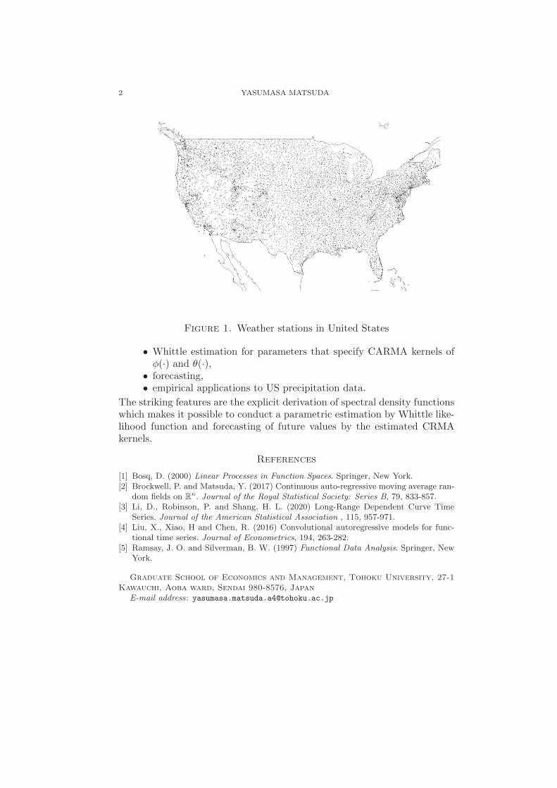
In this talk, we propose a space-time autoregressive and moving average(ST-ARMA) model for spatio-temporal data, a discrete time series obser-vation of irregularly spaced data, denoted as Xt(s), s ∈ R

2, t = 1.2. . . ..Figure 1 shows observation points in US to record monthly precipitation,providing a typical example of spatio-temporal data. Regarding Xt(s) asa L2(R2)-valued time series, we construct a space-time ARMA(p, q) model,given by

Xt(s) =

p∑j=1

∫R2

φj(s− u)Xt−j(u)du+

q∑j=0

∫R2

θj(s− u)Lt−j(du),(1)

s ∈ R2, t = 0,±1,±, 2, . . . ,

where Lt(u) is a Levy sheet on R2 independent across t, and φ(s) and θ(s) are

CARMA kernels in L2(R2). It is an temporal extension of continuous ARMArandom fields of Brockwell and Matsuda[2] by a convolutional operator of φand θ on L2(R2).

A space-time ARMA model is a kind of model for functional time series,a H2-valued time series for a Hilbert space H2. See Ramsay and Silverman[5] for independent cases, Bosq[1] for stationary time series cases, Liu et al.[4] for a pure AR model for L2[0, 1] valued time series, and Li et al. [3]for a semiparametric method to detect a long memory property in L2[0, 1]valued time series. One feature of ST-ARMA model in (1) is that it is aL2(R2)-valued time series model. It scauses several difficulty in establishingST-ARMA model properties that infinite region R

2 rather than the fixedinterval [0, 1]2 over which square integrable functions of Hilbert space isdefined.

We shall introduce the basic properties of space-time ARMA models givenas

• stationary conditions, more specifically, causal and invertible condi-tions,

• explicit form of spectral density functions,

Key words and phrases. CARMA random fields, Causality, Invertibility, Irregularlyspaced data, Levy sheet, Periodogram, Spectral density function, Whittle likelihood.

1

2 YASUMASA MATSUDA

Figure 1. Weather stations in United States

• Whittle estimation for parameters that specify CARMA kernels ofφ(·) and θ(·),

• forecasting,• empirical applications to US precipitation data.

The striking features are the explicit derivation of spectral density functionswhich makes it possible to conduct a parametric estimation by Whittle like-lihood function and forecasting of future values by the estimated CRMAkernels.

References

[1] Bosq, D. (2000) Linear Processes in Function Spaces. Springer, New York.[2] Brockwell, P. and Matsuda, Y. (2017) Continuous auto-regressive moving average ran-

dom fields on Rn. Journal of the Royal Statistical Society: Series B, 79, 833-857.

[3] Li, D., Robinson, P. and Shang, H. L. (2020) Long-Range Dependent Curve TimeSeries. Journal of the American Statistical Association , 115, 957-971.

[4] Liu, X., Xiao, H and Chen, R. (2016) Convolutional autoregressive models for func-tional time series. Journal of Econometrics, 194, 263-282.

[5] Ramsay, J. O. and Silverman, B. W. (1997) Functional Data Analysis. Springer, NewYork.

Graduate School of Economics and Management, Tohoku University, 27-1

Kawauchi, Aoba ward, Sendai 980-8576, Japan

E-mail address: yasumasa.matsuda.a4@tohoku.ac.jp