BAYESIAN SPATIAL AND SPATIO-TEMPORALMODELS FOR SKEWED AREAL COUNT DATA

BENARD CHERUIYOT TONUI

DOCTOR OF PHILOSOPHY(Applied Statistics)

JOMO KENYATTA UNIVERSITY OFAGRICULTURE AND TECHNOLOGY

2021

Bayesian Spatial and Spatio-temporal Models for Skewed ArealCount Data

Benard Cheruiyot Tonui

A Thesis Submitted in Partial Fulfillment of the Requirements forthe Degree of Doctor of Philosophy in Applied Statistics of the Jomo

Kenyatta University of Agriculture and Technology

2021

DECLARATION

This thesis is my original work and has not been presented for a degree in any other

University.

Signature: · · · · · · · · · · · · · · · · · · · · · · · · · · · Date: · · · · · · · · · · · · · · · · · ·

Benard Cheruiyot Tonui

This thesis has been submitted for examination with our approval as University Super-

visors.Signature: · · · · · · · · · · · · · · · · · · · · · · · · Date: · · · · · · · · · · · · · · · · · · · · ·

Prof. Samuel Mwalili, PhD

JKUAT, Kenya

Signature: · · · · · · · · · · · · · · · · · · · · · · · · Date: · · · · · · · · · · · · · · · · · · · · ·

Dr. Anthony Wanjoya, PhD

JKUAT, Kenya

ii

DEDICATION

To my sons Felix, Collins, Alex and Arnold

iii

ACKNOWLEDGEMENTS

I would like to acknowledge very important persons who, before and during the course

of my PhD, have contributed through diverse ways to the success of this thesis. First

of all, I will credit God for being my guide, providing renewed strength each day

throughout my entire life.

I wish to thank my supervisors Prof. Samuel Mwalili and Dr. Anthony Wanjoya

of JKUAT for the wonderful years of great supervision. Your guidance, support, sug-

gestions and contributions are beyond par. It has been a delightful privilege and honor

to have learnt from and been mentored by such great minds. I am forever grateful. In

a special way, I am grateful to all the members of the Statistics and Actuarial Science

department, JKUAT, for the guidance I received at all the presentations, towards my

progress, organized through the department.

I also appreciate and acknowledge the support of my employer, University of Ka-

bianga, through the study leave to enable me conduct my research and finalize on data

analysis and the thesis write up. In particular, I would like to thank the Head of Math-

ematics & Computer Science department, Dr. D. Adicka, for allowing me to proceed

on the study leave. I am also thankful to Prof. M. Oduor, the Dean School of Science

and Technology, who yearned to see the successful completion of my work. The sup-

port of my colleague, Dr. R. Langat, cannot go unnoticed as he has mentored me since

my high school days and later on introducing me to the field of Statistics.

This thesis will not have been possible without the support of my family. My very

special thanks go to my beloved wife, Caro, for the inspirational and endless care and

for the many sacrifices during the entire period of my PhD studies. To my elder brother,

Kipkoech Tonui, I thank you so much for the financial support and seeing me through

my early education. Thank you for motivating me to pursue a career in mathematics;

it has been a very interesting and inspiring journey. I am pleased with the number of

opportunities that have come my way ever since. Finally, to my dearest mum, Eliza-

beth, I am grateful for your unwavering efforts and for sacrificing everything to ensure

that I pursue my dream.

iv

TABLE OF CONTENTS

DECLARATION . . . . . . . . . . . . . . . . . . . . . . . . . . . . . . . . . ii

DEDICATION . . . . . . . . . . . . . . . . . . . . . . . . . . . . . . . . . . iii

ACKNOWLEDGEMENTS . . . . . . . . . . . . . . . . . . . . . . . . . . . iv

TABLE OF CONTENTS . . . . . . . . . . . . . . . . . . . . . . . . . . . . vii

LIST OF TABLES . . . . . . . . . . . . . . . . . . . . . . . . . . . . . . . . viii

LIST OF FIGURES . . . . . . . . . . . . . . . . . . . . . . . . . . . . . . . ix

LIST OF APPENDICES . . . . . . . . . . . . . . . . . . . . . . . . . . . . x

ABBREVIATIONS AND ACRONYMS . . . . . . . . . . . . . . . . . . . . xi

ABSTRACT . . . . . . . . . . . . . . . . . . . . . . . . . . . . . . . . . . . xiii

CHAPTER ONE . . . . . . . . . . . . . . . . . . . . . . . . . . . . . . . . . 1

INTRODUCTION. . . . . . . . . . . . . . . . . . . . . . . . . . . . . . . . . . . . . . . . . 1

1.1 Overview of Spatial and Spatio-temporal data . . . . . . . . . . . . . . . 1

1.2 Disease Mapping . . . . . . . . . . . . . . . . . . . . . . . . . . . . . . 2

1.3 Statement of the Problem . . . . . . . . . . . . . . . . . . . . . . . . . . 3

1.4 Objectives of the Study . . . . . . . . . . . . . . . . . . . . . . . . . . . 4

1.4.1 General Objective . . . . . . . . . . . . . . . . . . . . . . . . . . . . . 4

1.4.2 Specific Objectives . . . . . . . . . . . . . . . . . . . . . . . . . . . . 4

1.5 Justification of the Study . . . . . . . . . . . . . . . . . . . . . . . . . . 4

1.6 Kenya HIV and AIDS data set . . . . . . . . . . . . . . . . . . . . . . . 4

1.7 Thesis Outline . . . . . . . . . . . . . . . . . . . . . . . . . . . . . . . . 5

CHAPTER TWO . . . . . . . . . . . . . . . . . . . . . . . . . . . . . . . . 7

v

LITERATURE REVIEW. . . . . . . . . . . . . . . . . . . . . . . . . . . . . . . . . . . . . . . . . 7

2.1 Bayesian Hierarchical Disease Mapping Models . . . . . . . . . . . . . . 7

2.1.1 Poisson-gamma Model . . . . . . . . . . . . . . . . . . . . . . . . . . 10

2.1.2 Poisson-lognormal Model . . . . . . . . . . . . . . . . . . . . . . . . 11

2.1.3 Spatial Gaussian Conditional Autoregressive Models . . . . . . . . . . 11

2.1.4 Intrinsic Conditional Autoregressive Model . . . . . . . . . . . . . . . 12

2.1.5 Proper Conditional Autoregressive model . . . . . . . . . . . . . . . . 13

2.1.6 Leroux Conditional Autoregressive Model . . . . . . . . . . . . . . . . 14

2.1.7 Convolution Model . . . . . . . . . . . . . . . . . . . . . . . . . . . . 14

2.2 Skew-Random Effect Distributions in Disease Mapping . . . . . . . . . . 15

2.3 Skew-t Spatial Combined Random Effects Model . . . . . . . . . . . . . 15

2.4 Spatio-temporal Models for Disease Mapping . . . . . . . . . . . . . . . 17

CHAPTER THREE . . . . . . . . . . . . . . . . . . . . . . . . . . . . . . . 20

RESEARCH METHODOLOGY. . . . . . . . . . . . . . . . . . . . . . . . . . . . . . . . . . . . . . . . . 20

3.1 Skew-Random Effect Distributions in Disease Mapping . . . . . . . . . . 20

3.1.1 Skew-normal Distribution . . . . . . . . . . . . . . . . . . . . . . . . 20

3.1.2 Skew-t Distribution . . . . . . . . . . . . . . . . . . . . . . . . . . . . 21

3.2 Skew-t Spatial Combined Random Effects Model for Areal Count Data . 22

3.3 Spatio-temporal Models for Disease Mapping . . . . . . . . . . . . . . . 25

3.3.1 Parametric Linear time trend models . . . . . . . . . . . . . . . . . . . 26

3.3.2 Non-parametric dynamic time trend models . . . . . . . . . . . . . . . 26

3.3.3 Prior distributions . . . . . . . . . . . . . . . . . . . . . . . . . . . . . 28

3.4 Bayesian Model Estimation Methods . . . . . . . . . . . . . . . . . . . . 29

3.4.1 Markov chain Monte Carlo . . . . . . . . . . . . . . . . . . . . . . . . 30

3.4.2 Integrated Nested Laplace Approximation . . . . . . . . . . . . . . . . 32

3.5 Bayesian Model Comparison . . . . . . . . . . . . . . . . . . . . . . . . 36

CHAPTER FOUR . . . . . . . . . . . . . . . . . . . . . . . . . . . . . . . . 39

RESULTS AND DISCUSSIONS. . . . . . . . . . . . . . . . . . . . . . . . . . . . . . . . . . . . . . . . . 39

vi

4.1 Application of Skew-Random Effects Model to HIV and AIDS Data . . . 39

4.2 Simulation Study for Skew-Random Effects models . . . . . . . . . . . . 40

4.3 Application of Skew-t Spatial Combined Random Effects model to HIV

and AIDS Data . . . . . . . . . . . . . . . . . . . . . . . . . . . . . . . 44

4.4 Simulation study for Skew-t Spatial Combined Random Effects Model . . 47

4.5 Spatio-temporal Variation of HIV and AIDS Infection in Kenya . . . . . . 49

CHAPTER FIVE . . . . . . . . . . . . . . . . . . . . . . . . . . . . . . . . 56

CONCLUSION AND RECOMMENDATIONS. . . . . . . . . . . . . . . . . . . . . . . . . . . . . . . . . . . . . . . . . 56

5.1 Conclusion . . . . . . . . . . . . . . . . . . . . . . . . . . . . . . . . . 56

5.2 Recommendations for Further Research . . . . . . . . . . . . . . . . . . 57

REFERENCES . . . . . . . . . . . . . . . . . . . . . . . . . . . . . . . . . . 58

APPENDICES . . . . . . . . . . . . . . . . . . . . . . . . . . . . . . . . . . 68

vii

LIST OF TABLES

Table 3.1: Specification and rank deficiency for different space-time interactions 27

Table 4.1: Parameter estimates for the models . . . . . . . . . . . . . . . . . 39

Table 4.2: Simulation study: average MSE values (bold = lowest) . . . . . . 43

Table 4.3: Simulation study: DIC values (bold = lowest) . . . . . . . . . . . . 44

Table 4.4: Summary statistics for 2016 HIV and AIDS in Kenya . . . . . . . 44

Table 4.5: Parameter estimates for the models . . . . . . . . . . . . . . . . . 46

Table 4.6: Simulation study: average MSE values (bold = lowest) for setting

A (large UH, small CH) and setting B (small UH, large CH) . . . . . 48

Table 4.7: Simulation study: DIC values (bold = lowest) for setting A (large

UH, small CH) and setting B (small UH, large CH) . . . . . . . . . . 49

viii

LIST OF FIGURES

Figure 4.1: HIV and AIDS relative risk map (a) and the 95% lower (b) and

upper (c) credible limits maps for the Skew-t model . . . . . . . . . . 41

Figure 4.2: Standardized incidence rates for 2016 HIV and AIDS in Kenya . . 45

Figure 4.3: The spatial pattern of HIV and AIDS incidence risks ζi = exp(ui)

(a); Posterior probabilities P (ζi > 1|Y ) (b) . . . . . . . . . . . . . . . 50

Figure 4.4: Global linear temporal trend of HIV and AIDS incidence risks.

Solid line: posterior mean for βt; Dashed lines: 95% credibility intervals 51

Figure 4.5: Temporal trend of HIV and AIDS incidence risks . . . . . . . . . 52

Figure 4.6: Specific temporal trends for selected counties: Homa Bay, Bomet,

Nairobi and Wajir. . . . . . . . . . . . . . . . . . . . . . . . . . . . . 53

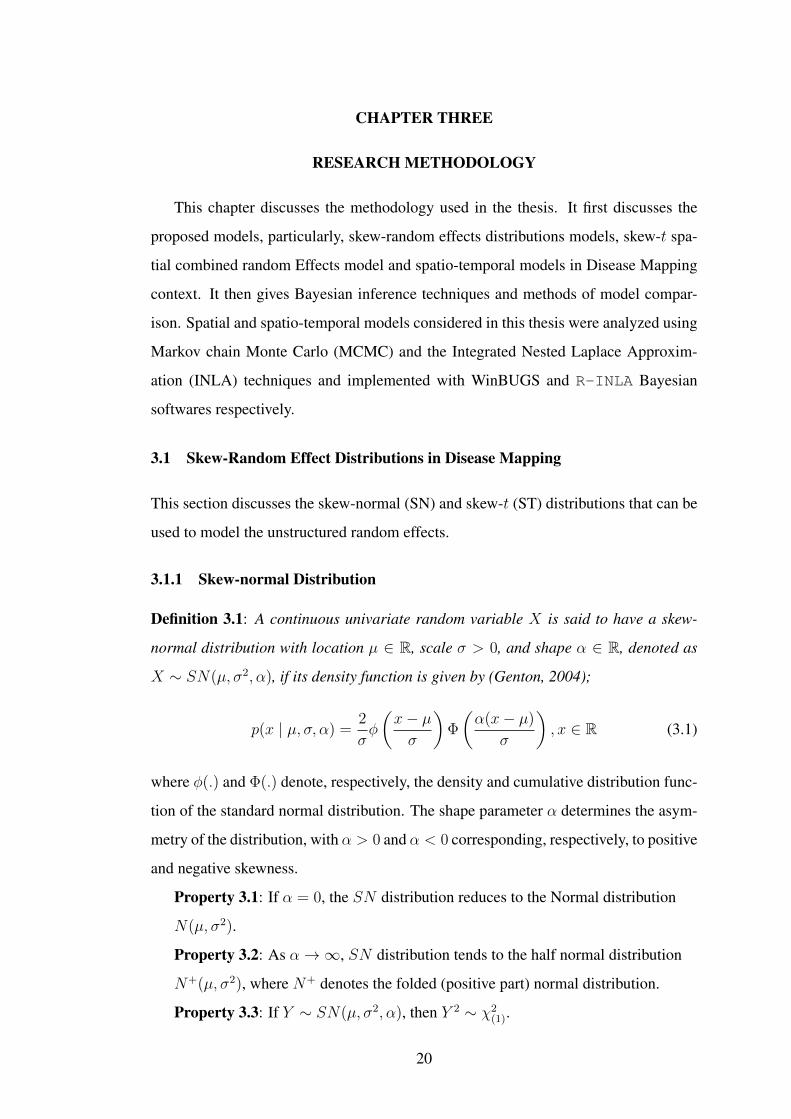
Figure 4.7: Posterior mean of the spatio-temporal interaction δi: Type I Inter-

action . . . . . . . . . . . . . . . . . . . . . . . . . . . . . . . . . . 54

Figure 4.8: Posterior mean of the spatio-temporal interaction δi: Type II Inter-

action . . . . . . . . . . . . . . . . . . . . . . . . . . . . . . . . . . 54

Figure 4.9: Posterior mean of the spatio-temporal interaction δi: Type III In-

teraction . . . . . . . . . . . . . . . . . . . . . . . . . . . . . . . . . 55

Figure 4.10: Posterior mean of the spatio-temporal interaction δi: Type IV In-

teraction . . . . . . . . . . . . . . . . . . . . . . . . . . . . . . . . . 55

ix

LIST OF APPENDICES

Appendix 1: RR estimates for the 2016 HIV and AIDS in Kenya . . . . . . . . 68

Appendix 2: WinBugs code for Skew-t Model . . . . . . . . . . . . . . . . . 69

Appendix 3: WinBugs code for Skew-t Spatial Combined Random Effects Model 71

Appendix 4: R-INLA codes for Spatio-temporal Analysis of HIV and AIDS

in Kenya . . . . . . . . . . . . . . . . . . . . . . . . . . . . . . . . . . . . 74

Appendix 5: List of Publications from the Thesis . . . . . . . . . . . . . . . . 81

x

ABBREVIATIONS AND ACRONYMS

BYM Besag, York and Molli´e

CAR Conditional Autoregressive

CH Correlated Heterogeneity

CON Convolution

DIC Deviance Information Criterion

EB Empirical Bayes

FB Fully Bayes

GLM Generalized Linear Models

GLMM Generalized Linear Mixed Models

GMRF Gaussian Markov Random Field

GOF Goodness-of-fit

GPS Global Positioning System

HIV Human Immunodeciency Virus

ICAR Intrinsic Conditional Autoregressive

ICAR CH Intrinsic Conditional Autoregressive Correlated Heterogeneity

ICAR CON Intrinsic Conditional Autoregressive Convolution

INLA Integrated Laplace Approximation

KEMRI Kenya Medical Research Institute

KNBS Kenya National Bureau of Statistics

xi

MCMC Markov chain Monte Carlo

MSPE Mean Squared Predictive Error

NACC National AIDS Control Council

NASCOP National AIDS and STI Control Programme

NCAPD National Council for Population and Development

pCAR Proper Conditional Autoregressive

pCARCOM Proper Conditional Autoregressive Combined

pD Effective number of parameters

PG Poisson-Gamma

PLN Poisson-lognormal

PLHIV People Living with HIV

PLSN Poisson-log-skew-normal

PLST Poisson-log-skew-t

PLT Poisson-log-t

PMTCT Prevention of Mother to Child Transmission

LCAR Leroux Conditional Autoregressive

RR Relative Risk

SIR Standardized Incidence Rate

SN Skew-normal

ST Skew-t

STCAR Skew-t Conditional Autoregressive

STCARCOM Skew-t Conditional Autoregressive Combined

UH Uncorrelated Heterogeneity

xii

ABSTRACT

Disease mapping models have found wide range of applications to epidemiology andpublic health. These models typically extend from generalized linear models (GLM)and are usually implemented using a Bayesian approach. Most of the disease mappingmodels incorporate random effects that assume either a Gaussian exchangeable priorfor the spatially unstructured heterogeneity or the popular Gaussian CAR priors forthe spatially structured variability. However, this Gaussian assumption is often viol-ated since random effects can be skewed. This thesis proposed models that relax theusual normality assumption on the spatially unstructured random effect by using skewnormal and skew-t distributions. In the analysis of 2016 HIV and AID data in Kenya,it was found out that models whose unstructured random effects follow asymmetricskewed distributions perform better than models with corresponding symmetric dis-tributed unstructured random effects. Classical random-effects models for count dataincludes the Poisson-gamma model, that utilizes the conjugate feature between thePoisson and Gamma distributions to attain closed-form posterior distribution but ac-counts only for overdispersion or extra variation, and the Gaussian conditional autore-gressive (CAR) models, that model spatial correlation but does not have a closed-formposterior distribution. This thesis also considers an alternative model that combinesa Poisson-gamma model with a spatially structured skew-t random effect in the samemodel thus accounting for the extra variability, spatial correlation and skewness in thedata. In the analysis of 2016 Kenya HIV and AIDS data, the skew-t spatial combinedrandom effects model was found to provide a better alternative to the classical diseasemapping models. Simulation studies also show that the proposed models perform bet-ter than the classical disease mapping models. To model spatio-temporal variation,this thesis considered Leroux CAR (LCAR) prior for spatial random effect and im-plemented Bayesian analysis using integrated nested Laplace approximations (INLA).In the analysis of spatio-temporal variation of HIV and AIDS in Kenya for the period2013–2016, it was found out that counties located in the Western region of Kenya showsignificantly higher HIV and AIDS risks as compared to the other counties.

xiii

CHAPTER ONE

INTRODUCTION

1.1 Overview of Spatial and Spatio-temporal data

Spatial and spatio-temporal data have become more accessible in the recent past mainly

due to the availability of computational tools which has made collection of real-time

data from sources like GPS and satellites possible (Lawson and Lee, 2017; Arab,

2015). Therefore, the researchers in various fields like epidemiology, ecology, cli-

matology and social sciences frequently encounter geo-referenced data which capture

information about space and also possibly time. Spatial and spatio-temporal modeling

play a very important role in various studies which include disease mapping. Hier-

archical spatial and spatio-temporal models often offer a flexible approach for mod-

eling spatially correlated and temporally dependent count data. This thesis considers

Bayesian hierarchical spatial and spatio-temporal disease mapping models and their

extensions with application to modeling HIV and AIDS data.

Data whose location in space is known (i.e, geographically referenced) are referred

to as spatial data. Banerjee et al. (2015) defined spatial data as realizations of stochastic

process indexed by space

Y (s) = {y(s), s ∈ D} (1.1)

where D ⊂ Rd (d = 2 or 3) with spatial coordinates s = (s1, ..., sd)′.

Spatial stochastic processes vary in the plane with d = 2 and the coordinates are

given by the ordered pair s = (x, y)′ (i.e, longitude and latitude). The spatial process

can be easily extended to the spatio-temporal case including a time component so that

the data are now defined by a process indexed by a set on a space-time manifold with

d = 3 and their coordinates are given by s = (x, y, t)′. That is, for observations made

at n spatial areas or locations and at time point t;

Y (s, t) ={y(s, t), (s, t) ∈ D ⊂ R3

}(1.2)

In general, stochastic processes with d ≥ 2 are referred to as random fields.

Spatial data sets can be classified into one of the following three basic types:

1

(i) Areal or lattice data: This is where data values y(s1), ..., y(sn) are observations

associated with a fixed number of areal units (area objects) that may form a regu-

lar lattice, as in the case of remotely sensed images, or be a set of irregular areas

or zones based on administrative boundaries, such as districts, counties, census

zones, regions or even countries. Often y(s) represents a suitable summary like

the number of observed cases in each area and is referred to as areal or lattice data.

In this case, the interest is usually on mapping or smoothing an outcome over the

domain D.

(ii) Point-Referenced or geostatistical data: This relates to variables which change

continuously in space and whose observations have been sampled at a predefined

and fixed set of point locations. For example, a realization of the air pollution

process y(s) in which a collection of air pollutant measurements are obtained by

monitors located in the set (s1, s2, · · · , sn) of n points (rather than areas) is often

referred to as point-referenced or geostatistical data.

(iii) Spatial Point pattern data: This refers to data set consisting of a series of point

locations in some study region, at which events of interest have occurred, such

as cases of a disease or incidence of a type of crime. Here, y(s) represents the

occurrence or not of an event such that it takes the values 0 or 1 and locations

s ∈ Rd are random. Such data are referred to as Spatial Point pattern data

For exhaustive documentation of each type of spatial data and comprehensive theor-

etical foundations, see for example Banerjee et al. (2015), Gelfand et al. (2010) and

Cressie (1993).

If the data considered are available at the area level and consist of aggregated counts

of outcomes and covariates, typically disease mapping and/or ecological regression can

be specified (Richardson, 2003; Lawson et al., 2009).

1.2 Disease Mapping

Disease mapping is the study of the geographical or spatial distribution of health out-

comes. In disease mapping, the objective of analysis is usually to estimate the true

relative risk of a disease of interest across a geographical study area. Disease mapping

2

is useful for several purposes such as health services resource allocation, disease at-

las construction, detection of clustering of a disease and in formulation of hypotheses

about disease aetiology. Several statistical reviews on disease mapping have been done

(Hu et al., 2020; Coly et al., 2019; Riebler et al., 2016; Wakefield, 2007; Lawson, 2001;

Bithell, 2000).

1.3 Statement of the Problem

Methods for mapping diseases has progressed considerably in recent years. These

models basically, utilize random effects that are partitioned into spatially correlated

and uncorrelated components. In the analysis of areal data, the spatially uncorrelated

random effects are mainly modelled using a Gaussian exchangeable prior. In prac-

tice, however, epidemiological or disease data is often observed to be non-normal,

potentially limiting the degree to which Gaussian random effects models can be appro-

priately fit to data. This thesis, thus, considered models that allow for random effect

distributions that are highly skewed or have excess kurtosis. Therefore, we investigated

disease mapping models in which the spatially unstructured heterogeneity is modelled

using skew-normal (SN) or skew-t (ST) distributions while spatially structured hetero-

geneity is modelled with a skew-t spatial random effect distribution. In addition, to

account for overdispersion in spatially correlated and also possibly skewed data, this

thesis considered an alternative model that combines a Poisson-gamma model with a

spatially structured skew-t random effect in the same model; thus, accounting for the

extra variability, spatial correlation and skewness in the data. This thesis also con-

sidered more efficient spatio-temporal models for such data. This was necessitated by

the availability of data recorded for different regions over a period of time. This in-

volved use of the recently developed strategy for Bayesian inference called integrated

nested Laplace Approximation (INLA); INLA allows fairly complex models to be fit

much faster than the popular Markov chain Monte Carlo (MCMC) algorithms.

3

1.4 Objectives of the Study

1.4.1 General Objective

The main objective of this study is to develop flexible Bayesian spatial and spatio-

temporal hierarchical disease mapping models for skewed areal count data.

1.4.2 Specific Objectives

The specific objectives in this study are to:

(i) develop a disease mapping model with skew-random effect distributions for the

spatially unstructured random effects.

(ii) develop a Poisson-gamma model for spatially correlated and overdispersed skew

count data.

(iii) carry out simulation studies to assess the performance of the proposed models.

(iv) determine the spatio-temporal variation of HIV and AIDS infections in Kenya.

1.5 Justification of the Study

The disease mapping models developed in this study play an important role in address-

ing the spatio-temporal variation of HIV and AIDS in Kenya. Through these models,

the disease hot spot areas with extreme risks are identified. This is crucial in decision-

making related to health surveillance, which include optimal allocation of resources

for mitigation and prevention of disease in the affected areas.

1.6 Kenya HIV and AIDS data set

In Kenya the HIV and AIDS data is obtained from the national surveys: the Kenya

Demographic and Health Survey of 2003 (CBS and MOH, 2004), the Kenya AIDS

Indicator Survey 2007 (NASCOP, 2009), the Kenya Demographic and Health Sur-

vey of 2008/9 (KNBS, 2010), the Kenya AIDS Indicator Survey 2012 (NASCOP,

2014), the Kenya Demographic and Health Survey of 2014 (KNBS et al., 2015) and

4

the Kenya Demographic and Health Survey of 2017 (NASCOP et al., 2017). In addi-

tion, the Kenya HIV and AIDS data is supplemented by HIV testing among pregnant

women at Prevention of Mother to Child Transmission (PMTCT) program that has

been strengthened to cover wider area and is important in monitoring national trends

in the future. This data will provide good estimates of national HIV prevalence and the

trend.

This HIV and AIDS data aims to offer source for understanding the HIV epidemic

in Kenya, in order to provide important insights into the impact of the HIV epidemic.

This study focuses only on HIV cases among adults, that is, men and women aged

15-64 years. The data set is used in Chapter Four to illustrate and compare various

disease mapping models proposed in Chapters Three. These comparison are in terms

of cross-sectional and trend estimate of the HIV epidemic in Kenya. The results are

then presented in the form of prevalence, incidence, relative risks and posterior prob-

abilities.

1.7 Thesis Outline

This thesis aims at development of Bayesian hierarchical spatial and spatio-temporal

disease mapping models. The thesis is structured in form of Chapters and it comprises

of five chapters described below.

Chapter One serves as an introduction to the study. It gives an overview of the

thesis and brief introduction to the concepts of Spatial Statistics and disease map-

ping. A statement of the problem and the objectives of the study are also given in this

Chapter.

Chapter Two covers literature review in which statistical reviews and recent de-

velopments in spatial and spatio-temporal disease mapping are considered. First, an

overview of classical disease mapping models is given. It then gives extensions of the

classical disease mapping models. In particular, models with non-Gaussian random ef-

fect distributions, skew-t spatial combined random effects model and spatio-temporal

models are discussed.

Chapter Three gives the methodology used in the thesis. First, this chapter ex-

tends the classical disease mapping models by introducing more flexible distributions

5

for the spatially unstructured random effects. In particular, the skew-normal and skew-

t distributions are discussed. Skew-t spatial combined random effects model for count

data is presented in this chapter. This model is based on the so-called combined model

and it uses a single framework to capture overdispersion, spatial correlation and the

skewness in the data. Then Spatio-temporal models for disease mapping are discussed,

in which linear time trend and non-parametric dynamic time trend models are explored.

Various space-time interaction models are also given. Bayesian inference techniques

are also discussed. In particular, the MCMC and INLA techniques are discussed. Fi-

nally, methods for Bayesian model comparison and goodness of fit (GOF) are also

explored in this chapter. In particular, the effective number of parameters (pD), devi-

ance information criterion (DIC) and the mean squared predictive error (MSPE) are

discussed.

Chapter Four gives results and discussions on the applications of the proposed

models to HIV and AIDS data. First, the use of the skew-normal and skew-t distri-

butions is investigated and applied to 2016 Kenya HIV and AIDS data. The skew-

distributions allows for the flexibility of random-effects distribution to adjust for the

deviation from the usual normality assumption. Secondly, application of skew-t spatial

combined random effects model to 2016 Kenya HIV and AIDS data is then presented.

Then spatio-temporal variation of HIV in Kenya is given in which various space-time

interaction models are given and fitted to the 2013-2016 Kenya HIV data set. Simu-

lation studies to assess the performance of the proposed models are also presented in

this chapter.

Chapter Five provides general conclusions of the main results and the recom-

mendations for further research. List of references is given at the end of the thesis.

6

CHAPTER TWO

LITERATURE REVIEW

Disease mapping models and analysis have attracted tremendous growth in the

recent past both in the methodological and applications aspects. This chapter reviews

the literature about Bayesian hierarchical disease mapping models. First, it gives an

overview of the Bayesian hierarchical disease mapping models. Secondly, it discusses

non-Gaussian random effects distributions in disease mapping. It then discusses the

skew-t spatial combined random effects model and spatio-temporal models for disease

mapping.

2.1 Bayesian Hierarchical Disease Mapping Models

Over the past decades and with the advent of computational methods and statistical

methodology, and availability of spatially-referenced data and fast software tools, dis-

ease mapping has increased in popularity in epidemiological research (Lawson and

Lee, 2017; Ugarte et al., 2017; Riebler et al., 2016; Elliott and Wartenberg, 2004).

Suppose the study region is divided into n areas labeled i = 1, 2, ..., n. Let Yi be

the observed count of disease in the ith area, Ei denote the expected count in the ith

area and ωi be the unknown relative risk in that area. Here the expected counts are

assumed to be known constants. The standardized incidence ratio (SIR) is usually the

basic technique use to estimate the relative risk of a disease for a given area i (Neyens

et al., 2012). SIR is defined as the ratio of observed counts to the expected counts:

ωi = SIRi = YiEi

. If ωi = SIRi > 1 in a given area, then the risk of the disease is higher

than expected for that region while ωi < 1 will imply a lower risk of the disease than

expected for that area. However for the case of a rare disease and very low populated

areas, the expected counts Ei can be very low which may results in unnecessarily high

risk of the disease for that respective areas. Another assumption is that the areas under

study are independent, which is often not practically realistic in most epidemiological

studies. Therefore the use of SIR estimates do not capture the extra variability or

spatial correlation due to unobserved heterogeneity present in the data (Neyens et al.,

2012).

7

To overcome this problem, Bayesian hierarchical spatial models can be used so

that the joint posterior distribution for process and parameters given data can be ob-

tained (Coly et al., 2019). Such models allow the use of covariates that can provide

information on the risk of mortality, as well as a set of random effects that capture

the dependence between neighbouring regions (Lawson and Lee, 2017). Bayesian es-

timation procedure has several potential advantages as compared to the classical (e.g.

maximum likelihood) estimation procedures. First, Bayesian inference allows us to

express uncertainty about model parameters through prior distributions. Secondly, the

availability of advanced softwares for Bayesian analysis such as WinBUGS (Spiegel-

halter et al., 2002) for MCMC algorithm and R-INLA (Martino and Rue, 2009) for

INLA technique provide a flexible way to model complex disease mapping models.

Disease mapping models basically extends from the generalized linear models

(GLM). Suppose Yi are the counts of disease cases observed for a set of regions

i = 1, ..., n partitioning a study domainD. The counts are normally modeled as either

Poisson or Binomial random variables in the GLM framework, using a log or logit link

function, respectively (Coly et al., 2019; Kassahun et al., 2012; Molenberghs et al.,

2010; Agresti, 2002). For modeling rare diseases, the appropriate model to use is the

Poisson model. When the values of region-specific fixed covariates xi with associated

parameters β are observed, these can be included in the model in the GLM manner.

Overdispersion or spatial correlation due to unobserved heterogeneity present in

count data is usually not captured by simple covariate models and it is often appropri-

ate to include some additional term or terms in a model in order to capture such effects.

Basically, overdispersion or extra-variation can be accommodated by either inclusion

of a prior distribution for the relative risk (such as a Poisson-gamma model) or by

extension of the linear or non-linear predictor term to include an extra random effect

(log-normal model). The later leads to a hierarchical generalized linear mixed model

(GLMM) with one set of random effects (Lawson and Lee, 2017; Riebler et al., 2016),

often modeled with Gaussian exchangeable prior distributions. In Bayesian setting,

the model is specified in a hierarchical structure which allows the overall distribution

of Yi to be defined in two stages. At the first stage, observations Yi are conditionally

independent given the values of the random affects. The second stage specify the dis-

8

tribution of the random effects thus allowing a mechanism for inducing extra-Poisson

variability in the marginal distribution of the Y ′i s.

Correlated random effects can be introduced using a spatial covariance matrix. This

can be achieved by considering the random effects to form a single vector following

an appropriate distribution with a specified mean and a spatial variance-covariance

matrix. There are two approaches of defining spatially structured prior formulation of

the random effects. The most popular is the multivariate Gaussian distribution (Waller

and Gotway, 2004; Gaetan and Guyon, 2010; Sherman, 2011). The spatial variance-

covariance matrix is made up of parametric functions defining the covariance structure

based on location of any two units of study. In the case of areal data, the neighbourhood

structure can be specified based on the basis of sharing a border, the distance between

the centroids of any pair of regions or a combination of these two (Waller and Gotway,

2004; Cressie, 1993).

Clayton and Kaldor (1987) modified the hierarchical structure by replacing the set

of exchangeable priors at the second stage with a spatially structured prior distribution,

leading to local empirical Bayes estimates obtained as a weighted average of observa-

tions of neighboring regions thus borrowing strength locally rather than globally. As

an alternative to multivariate Gaussian models, Besag et al. (1991) extended the ap-

proach to a fully Bayesian setting using the MCMC algorithm. Their model is called

conditional autoregressive (CAR) model.

In the CAR formulation, conditional distribution of a random effect in a region

given all the other random effects is simply the weighted average of all the other ran-

dom effects. Besag et al. (1991) assigned the weights based on whether a pair of

regions shared a boundary or not; if the regions share a boundary, the weight is 1,

otherwise it is 0. Other weighting possibilities include Leroux et al. (1999), MacNab

and Dean (2000) and Green and Richardson (2002). The CAR formulation has com-

putational advantage over the multivariate Gaussian distribution in the sense that the

variance component in multivariate Gaussian requires matrix inversion at each update

when executing the algorithm during estimation, leading to more computational burden

which is not the case in CAR.

Up to this far, models borrowing strength either globally or locally have been dis-

9

cussed. Besag et al. (1991) suggested the inclusion of both spatially structured and

spatially unstructured random effects in the same model through a convolution prior

so that the model allows borrowing of information both locally and globally. There-

fore they proposed the popular Besag-York-Molli´e model (BYM) model in which the

unstructured random effect assumes a Gaussian exchangeable prior while the spatially

structured random effect assumes an intrinsic conditional autoregressive (ICAR) prior.

There is an extensive literature in Bayesian hierarchical disease mapping models

that have been used to estimate disease relative risks. In these models, covariates and

a set of random effects can be included so as to respectively provide more information

on the incidence risk and account for the correlation between the neighbouring ares.

The following subsections outline the classical Bayesian hierarchical disease mapping

models.

2.1.1 Poisson-gamma Model

A Poisson-gamma (PG) model is a mixed model obtained by allowing the Poisson

mean to have a gamma distribution. It is defined as (Lawson and Lee, 2017):

Yi ∼ Poisson(Eiωi);

ωi ∼ Gamma(a, b)(2.1)

where Yi and Ei denote, respectively, the observed and expected cases of disease in the

ith area (i = 1, ..., n); ωi is the the relative risk and the parameters a, b are assumed

to be fixed and known. Here, the mean and variance of the relative risk are given by

E(ω)i = a/b and V ar(ωi) = a/b2 (Lawson and Lee, 2017).

The Poisson-gamma model has been one of the popular models in disease mapping

due to its conjugacy feature that make it possible to obtain a closed form posterior

distribution (Neyens et al., 2012). However, this model only captures overdispersion or

uncorrelated heterogeneity (UH) but does not takes into account the spatial correlation

or correlated heterogeneity (CH) in the data. Additionally, this model does not provide

for the inclusion of covariate effects.

10

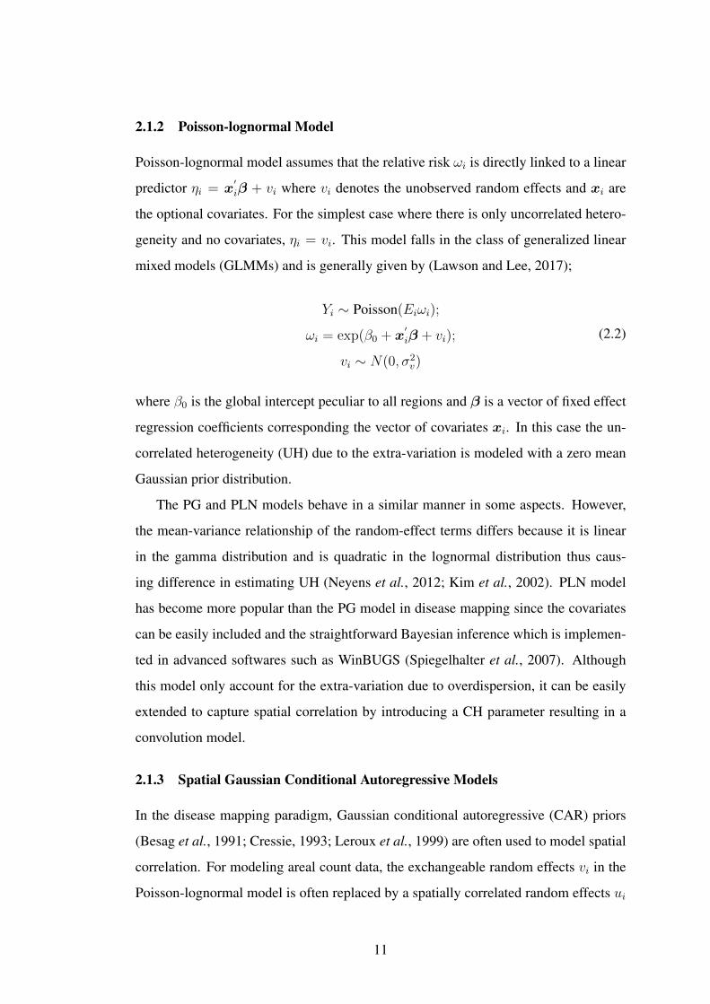
2.1.2 Poisson-lognormal Model

Poisson-lognormal model assumes that the relative risk ωi is directly linked to a linear

predictor ηi = x′iβ + vi where vi denotes the unobserved random effects and xi are

the optional covariates. For the simplest case where there is only uncorrelated hetero-

geneity and no covariates, ηi = vi. This model falls in the class of generalized linear

mixed models (GLMMs) and is generally given by (Lawson and Lee, 2017);

Yi ∼ Poisson(Eiωi);

ωi = exp(β0 + x′iβ + vi);

vi ∼ N(0, σ2v)

(2.2)

where β0 is the global intercept peculiar to all regions and β is a vector of fixed effect

regression coefficients corresponding the vector of covariates xi. In this case the un-

correlated heterogeneity (UH) due to the extra-variation is modeled with a zero mean

Gaussian prior distribution.

The PG and PLN models behave in a similar manner in some aspects. However,

the mean-variance relationship of the random-effect terms differs because it is linear

in the gamma distribution and is quadratic in the lognormal distribution thus caus-

ing difference in estimating UH (Neyens et al., 2012; Kim et al., 2002). PLN model

has become more popular than the PG model in disease mapping since the covariates

can be easily included and the straightforward Bayesian inference which is implemen-

ted in advanced softwares such as WinBUGS (Spiegelhalter et al., 2007). Although

this model only account for the extra-variation due to overdispersion, it can be easily

extended to capture spatial correlation by introducing a CH parameter resulting in a

convolution model.

2.1.3 Spatial Gaussian Conditional Autoregressive Models

In the disease mapping paradigm, Gaussian conditional autoregressive (CAR) priors

(Besag et al., 1991; Cressie, 1993; Leroux et al., 1999) are often used to model spatial

correlation. For modeling areal count data, the exchangeable random effects vi in the

Poisson-lognormal model is often replaced by a spatially correlated random effects ui

11

to obtain a spatial random effects model below.

Yi ∼ Poisson(Eiωi),

ωi = exp(β0 + x′iβ + ui

(2.3)

The joint distribution of the random effectsu = (u1, ..., un) often has a multivariate

normal distribution (Rampaso et al., 2016):

u ∼ MVN (µ,Σ) (2.4)

where µ is the mean vector and Σ = σ2uΦ is the variance covariance matrix which

determines the spatial structure; σ2u is the variance parameter and Φ is the precision

matrix given by Φ = (I − ρW )−1M , where I is a n × n identity matrix, ρ is a

parameter that measures spatial correlation; W is a non-negative symmetric n × n

spatial proximity or weight matrix with zero elements on its diagonal, that is wii = 0

and wij = 1 if the ith and jth areas are neighbours (i ∼ j) and 0 otherwise; M is a

diagonal matrix, that is M = Mii = diag(ni), where ni is the number of neighbours

of the ith area.

The precision matrix Φ can be specified in various ways to give rise to different

CAR prior models.

2.1.4 Intrinsic Conditional Autoregressive Model

The Intrinsic conditional autoregressive (ICAR) model was proposed by Besag et al.

(1991) and is obtained by allowing the joint distribution of the random effects u to

have a multivariate normal distribution with mean vector 0 and variance matrix σ2uQ

−

(whereQ− is the generalized inverse ofQ), with the ijth element of matrixQ defined

by;

qij =

ni, if i = j

−1, if i ∼ j

0,Otherwise

(2.5)

:

The univariate full conditional distribution of ui given all the remaining compon-

12

ents u−i = (u1, ..., ui−1, ui+1, ..., un) is given by (Rampaso et al., 2016);

ui | u−i, σ2u ∼ Normal

(1

ni

n∑i∼j

uj,σ2u

ni

)(2.6)

The ICAR model, however, is improper and it treats the strength of spatial correlation

between random effects as maximum (ρ = 1) (MacNab, 2011; Botella-Rocamora

et al., 2013).

2.1.5 Proper Conditional Autoregressive model

Cressie (1993) proposed the proper conditional autoregressive (named pCAR here-

after) as an alternative approach for modeling different levels of spatial correlation. He

used a single set of random effects, but introduced a spatial smoothing parameter ρ that

measures spatial correlation by allowing the random effects u = (u1, ..., un) to have a

multivariate normal distribution with precision matrix Φ = D−1, that is,

u ∼ MVN(µ, σ2

uD−1)

(2.7)

so that the ijth element of matrixD defined by;

dij =

ni, if i = j

−ρ, if i ∼ j

0,Otherwise

(2.8)

If 0 ≤ ρ < 1,then the joint distribution of u in (2.7) is proper (Rampaso et al., 2016).

The univariate full conditional distribution for the random effects ui is given by (Lee,

2011):

ui | u−i, σ2u, ρ ∼ Normal

(ρ

ni

n∑i∼j

uj,σ2u

ni

)(2.9)

Taking ρ = 0 implies there is no spatial dependence and values of ρ closer to one

indicate strong spatial dependence in the data (ρ = 1 reduces to the ICAR model).

Rampaso et al. (2016) noted that for ρ close to zero, i.e when there is absence

of spatial dependence between the random effects, this model has a weakness in that

13

the conditional variance does not change and it continue to depend on the number of

neighbours ni.

2.1.6 Leroux Conditional Autoregressive Model

As an alternative to the ICAR and pCAR models, Leroux et al. (1999) proposed a

more general conditional autoregressive model (named LCAR hereafter) in which the

precision matrix is given by Φ = ρQ + (1 − ρ)I , where I is a n × n identity matrix

and the matrix Q is the same as defined in (2.5). It can be seen that for ρ = 0, LCAR

model reduces to a model with independent (exchangeable) random effects. As in the

pCAR mpodel, it reduces to the ICAR model when ρ = 1. If 0 ≤ ρ < 1, then the joint

distribution of u with precision matrix Φ = ρQ+ (1− ρ)I is proper (Rampaso et al.,

2016).

The univariate full conditional distribution is then given by (Lee, 2011);

ui | u−i, σ2u, ρ ∼ Normal

(ρ

(1− ρ) + niρ

n∑i∼j

uj,σ2

(1− ρ) + niρ

)(2.10)

2.1.7 Convolution Model

To model the random effects, Besag et al. (1991) also proposed another popular model

known as the convolution model (named BYM hereafter) which includes two sets of

random effects in the same model: a spatially unstructured component to account for

pure overdispersion and a spatially structured component to account for spatial correl-

ation:Yi ∼ Poisson(Eiωi),

ωi = exp(β0 + x′iβ + ui + vi),

ui ∼ ICAR(σ2u); vi ∼ N(0, σ2

v)

(2.11)

The BYM model is, however, improper and has identifiability problems (Eberly and

Carlin, 2000; MacNab, 2014; Rampaso et al., 2016). That is, each data point is repres-

ented by two random effects but only their sum ui + vi is only identifiable. In addition,

the Gaussian exchangeable prior in this model does not capture the extra variability

that may arise due to overdispersion.

14

2.2 Skew-Random Effect Distributions in Disease Mapping

The disease mapping models considered that have so far been considered have ran-

dom effects assuming either a Gaussian (normal) exchangeable prior for the spatially

unstructured heterogeneity or the popular Gaussian CAR priors for the spatially struc-

tured variability. However, this Gaussian assumption may be too restrictive because

some random effects can be skewed violating this general normality assumption (Nat-

hoo and Ghosh, 2012; Branco and Dey, 2001; Box and Tiao, 1973). Several authors

(Ngesa et al., 2014; Nathoo and Ghosh, 2012; Wakefield, 2007; Chen et al., 2002; Best

et al., 1999; Besag et al., 1991) have suggested that it is possible to replace this nor-

mality assumption with other choices such as the Laplace distribution, the Student t-

distribution or semi non-parametric (SNP) densities. For instance, Ngesa et al. (2014)

used generalized Gaussian distribution (GGD). Through a simulation, they found that

GGD performs better than the normal distribution. Thus there is a need to consider

models with more flexible non-Gaussian random effect distributions. This flexibility

could arise when the random effects distribution is highly skewed or has excess kur-

tosis. This thesis explores the use of skew-normal (SN) and skew-t (ST) distributions

as candidates for the spatially unstructured random effects. The SN and ST distribu-

tions fall in the general asymmetric class of skew-elliptical distributions (Branco and

Dey, 2001) which are often used to capture skewness and excess kurtosis in the data.

There is a rich literature on parametric modeling with skew-elliptical distributions. For

regression analysis using the multivariate skew-t distribution, see for example Branco

and Dey (2001), Sahu et al. (2003), and Azzalini and Capitanio (2003). To analyze spa-

tially correlated non Gaussian data, Kim and Mallick (2004) developed skew-normal

spatial Kriging process. In the context of non-Gaussian geostatistical data, Palacios

(2006) proposed a formulation using scale mixing of a stationary Gaussian process.

2.3 Skew-t Spatial Combined Random Effects Model

Overdispersed count data that is spatially correlated and also possibly skewed is a

common phenomenon in many practical situations. The classical random-effects mod-

els used for count data includes the Poisson-gamma model, that has a closed form

15

posterior distribution due to the conjugate feature between the Poisson and Gamma

distributions but accounts only for overdispersion or extra variation, and the Gaussian

conditional autoregressive (CAR) models, such as the intrinsic CAR model (Besag

et al., 1991), that model spatial correlation but does not have a closed-form posterior

distribution.

The popular convolution model (Besag et al., 1991) has been used to model both

correlated heterogeneity (CH) and uncorrelated heterogeneity (UH) in the data. This

model has been widely used in disease mapping studies because of its potential to

incorporate numerous weighting schemes (Neyens et al., 2012) and its implementation

in most Bayesian softwares such as WinBUGS (Spiegelhalter et al., 2007). However,

this model lacks the important conjugate feature offered by the Poisson-gamma model.

There are limited studies on count data models that utilize this conjugacy. Wolpert

and Ickstadt (1998) attempted to explore it by using correlated gamma field models.

However, (Best et al., 2005) noted poor performance of these models in simulation

study to compare various disease mapping models.

Neyens et al. (2012) proposed a model that combines a Poisson-gamma model with

normal random effects, thus accounting for both overdispersion and spatial correlation.

There are limited studies extending the Poisson-gamma model to accommodate spatial

correlation because of a number of reasons. First, a gamma distribution does not eas-

ily provide for extensions into covariate modeling, and, second, gamma distribution

does not take into account spatial correlation or correlated heterogeneity (CH). The

combined model provides a flexible way for introducing both the random effects and

covariate effects.

In the Neyens et al. (2012) spatial combined random effects model, spatial smooth-

ing is accomplished using a latent Gaussian Markov random field (MRF). This Gaus-

sian assumption is, however, too restrictive in practice to capture variability which can

be a problem in cases where there is high skewness and excess kurtosis. This thesis

considered an alternative model that combines a Poisson-gamma model with a spa-

tially structured skew-t random effect in the same model thus accounting for the extra

variability, spatial correlation and skewness in the data.

16

2.4 Spatio-temporal Models for Disease Mapping

Investigating only the spatial pattern of diseases or exposures as introduced above does

not allow us to say anything about their temporal variation which could be equally im-

portant and interesting. Modern registers nowadays provide a lot of information with

high quality data recorded for different regions over a period of time (i.e days, months

or years). This has brought in new challenges and goals which also require new and

more flexible statistical models, faster and less computationally demanding methods

for model fitting, and advance softwares to implement them. The spatial models intro-

duced above can be easily extended to model temporal variation by including a time

component so that the data are now defined by a process indexed by space and time.

Spatio-temporal disease mapping models are often used in disease surveillance studies

(Abellan et al., 2008; Lawson et al., 2009) where the objective is to identify the spatial

patterns and the temporal variation of disease risks or rates.

Spatio-temporal models are mainly used in disease mapping studies because they

provide a platform that enables borrowing of information from spatial and temporal

neighbours to reduce the high variability that is common to classical risk estimators,

such as the standardized mortality ratio (SMR) when the area of study has a low popu-

lation or the disease under consideration is rare. These models are usually formulated

in a hierarchical Bayesian framework and typically relies on generalized linear mixed

models (GLMM). Model fitting and statistical inference is commonly accomplished

through the empirical Bayes (EB) and fully Bayes (FB) approaches. The EB approach

usually relies on the penalized quasi-likelihood (PQL) (Breslow and Clayton, 1993),

while the FB approach usually uses Markov chain Monte Carlo (MCMC) techniques

(Gilks et al., 2005).

The FB approach has become more popular in disease mapping studies due to

the availability of advance Bayesian softwares such as WinBUGS Spiegelhalter et al.

(2002) for implementation of the MCMC procedure. However, there are many chal-

lenges in using the MCMC for Bayesian analysis. This includes the need to evaluate

convergence of posterior samples which often consumes a lot of time due to the ex-

tensive simulation. In addition, the MCMC methods may lead to large Monte Carlo

17

errors if the data at hand is huge and the models involved are complex or complicated

as in the case of spatio-temporal models (Schrodle et al., 2011). Further more, reli-

able inference may not be obtained if the priors of the hyperparameters are not chosen

correctly (Wakefield, 2007; Fong et al., 2010).

As an alternative to the MCMC, this study considered a new strategy called integ-

rated nested Laplace Approximation (INLA) which has been recently developed (Rue

et al., 2009) for Bayesian inference. INLA allows fairly complex models to be fit

much faster than the MCMC and is now becoming very popular in disease mapping.

In addition, INLA also has a package R-INLA (Martino and Rue, 2009) that can be

implemented easily in the free software R (R Core Team, 2016).

There is an extensive literature in Bayesian spatio-temporal disease mapping span-

ning parametric and non-parametric time trends models as well as interactions. For

example, see Bernardinelli et al. (1995); Assuncao et al. (2001) and Ugarte et al.

(2009a) for parametric models and Knorr-Held and Besag (1998) for non-parametric

time trends models. A major contribution to spatio-temporal disease mapping is the

research paper by Knorr-Held (2000), which describes four different types of space-

time interactions. Most studies in spatio-temporal disease mapping model both the

spatial and temporal effects using conditional autoregressive (CAR) priors, extending

the BYM (Besag et al., 1991) model. Recently, other approaches that includes the

use of splines have been proposed. For example, from an EB framework MacNab and

Dean (2001) considered autoregressive local smoothing in space and B-spline smooth-

ing for time. Ugarte et al. (2010) and Ugarte et al. (2012b) proposed a pure interac-

tion P-spline model for space and time, and Ugarte et al. (2012a) used an Analysis

of Variance (ANOVA) type P-spline model to study spatio-temporal variations of pro-

state cancer mortality in Spain. Within a FB framework, spline smoothing has also

been considered for disease mapping models, see for example MacNab and Gustafson

(2007) and MacNab (2007).

In this thesis, space-time disease mapping models were considered and fitted using

the INLA methodology. Most spatial and spatio-temporal disease mapping models that

have been implemented with INLA use the popular BYM convolution model (Besag

et al., 1991) in which the spatially structured random effect assumes an intrinsic con-

18

ditional autoregressive (ICAR) prior (Held et al., 2010; Schrodle et al., 2011; Schrodle

and Held, 2011a,b; Blangiardo et al., 2013). The ICAR prior is, however, improper

(MacNab, 2011; Botella-Rocamora et al., 2013) and the spatial and non-spatial ran-

dom effects in the BYM convolution model are not identifiable from the data (MacNab,

2014; Rampaso et al., 2016). In this thesis, the Leroux conditional autoregressive

(LCAR) prior proposed by Leroux et al. (1999) was used to model the spatially struc-

tured random effect in the spatial-temporal models considered. This prior has been

shown to perform better than the ICAR prior (Lee, 2011) and can be easily implemen-

ted with the R-INLA package.

19

CHAPTER THREE

RESEARCH METHODOLOGY

This chapter discusses the methodology used in the thesis. It first discusses the

proposed models, particularly, skew-random effects distributions models, skew-t spa-

tial combined random Effects model and spatio-temporal models in Disease Mapping

context. It then gives Bayesian inference techniques and methods of model compar-

ison. Spatial and spatio-temporal models considered in this thesis were analyzed using

Markov chain Monte Carlo (MCMC) and the Integrated Nested Laplace Approxim-

ation (INLA) techniques and implemented with WinBUGS and R-INLA Bayesian

softwares respectively.

3.1 Skew-Random Effect Distributions in Disease Mapping

This section discusses the skew-normal (SN) and skew-t (ST) distributions that can be

used to model the unstructured random effects.

3.1.1 Skew-normal Distribution

Definition 3.1: A continuous univariate random variable X is said to have a skew-

normal distribution with location µ ∈ R, scale σ > 0, and shape α ∈ R, denoted as

X ∼ SN(µ, σ2, α), if its density function is given by (Genton, 2004);

p(x | µ, σ, α) =2

σφ

(x− µσ

)Φ

(α(x− µ)

σ

), x ∈ R (3.1)

where φ(.) and Φ(.) denote, respectively, the density and cumulative distribution func-

tion of the standard normal distribution. The shape parameter α determines the asym-

metry of the distribution, with α > 0 and α < 0 corresponding, respectively, to positive

and negative skewness.

Property 3.1: If α = 0, the SN distribution reduces to the Normal distribution

N(µ, σ2).

Property 3.2: As α→∞, SN distribution tends to the half normal distribution

N+(µ, σ2), where N+ denotes the folded (positive part) normal distribution.

Property 3.3: If Y ∼ SN(µ, σ2, α), then Y 2 ∼ χ2(1).

20

Property 3.4: The mean and variance of Y ∼ SN(µ, σ2, α), are given by (Genton,

2004):

E(Y ) = µ+(

2π

) 12 α

V ar(Y ) = σ2 +(1− 2

π

)α2

(3.2)

3.1.2 Skew-t Distribution

Let Z ∼ SN(0, σ2, α) and X ∼ χ2v; v > 0 be independent independent random

variables. Then Y = µ + Z√X/v

is said to have a skew-t distribution with location

µ, scale σ, shape α and v degrees of freedom, denoted as Y ∼ ST (µ, σ2, α, v). The

density function of a skew-t random variable Y is given by (Nathoo and Ghosh, 2012):

p(y | µ, σ, α, v) = 2t(y;µ, σ, v)T

α(y − µ)

σ

(v + 1

(y−µ)2

σ2 + v

)1/2

; v + 1

(3.3)

where

t(y;µ, σ, v) =1

σ√πv

Γ {(v + 1)/2}Γ(v/2)

1[1 + (y−µ)2

vσ2

](v+1)/2,−∞ ≤ y ≤ ∞

That is, t(y;µ, σ, v) is the density of a student t− distribution with location µ, scale σ

and v degrees of freedom and T (.; v + 1) is the cumulative distribution function of a

standard t distribution on (v+ 1) degrees of freedom. The skew-t distribution contains

the following distributions as its special cases: normal (α = 0, v →∞), skew-normal

(v →∞) and student-t (α = 0).

The mean and variance of Y ∼ ST (µ, σ2, α, v), when they exist, are given by

(Azzalini and Capitanio, 2003):

E [Y | µ, σ, αv] = µ+σα√

1 + α2

(vπ

)1/2 Γ {(v − 1)/2}Γ(v/2)

, v > 1 (3.4)

V ar [Y | µ, σ, αv] = σ2

(v

v − 2− α2

1 + α2

v

π

Γ2 {(v − 1)/2}Γ2(v/2)

), v > 2 (3.5)

In order to assess the performance of the proposed models, the following following

21

models were fitted to the Kenya 2016 HIV and AIDS incidence data.

Yi ∼ Poisson(µi) (3.6)

with

1. PLN: log(µi) = log(Ei) + β0 + vi; vi ∼ N(0, σ2v)

2. PLSN: log(µi) = log(Ei) + β0 + φi; φi = δZi + vi; Zi ∼ N+(0;σ2z);

δ ∼ N(0, σ2δ ); vi ∼ N(0, σ2

v)

3. PLT: log(µi) = log(Ei) + β0 + φi; φi = η− 1

2i (vi); ηi ∼ Gamma(v

2, v

2);

vi ∼ N(0, σ2v)

4. PLST: log(µi) = log(Ei) + β0 + φi; φi = η− 1

2i (δZi + vi); Zi ∼ N(0;σ2

z);

δ ∼ N(0, σ2δ ); vi ∼ N(0, σ2

v)

where Yi and Ei denote, respectively, the observed and expected cases of HIV and

AIDS in the ith county (i = 1, ..., 47); δ is the skewness parameter; Z are skewing

variables and k is the number of degrees of freedom for the t distribution.

3.2 Skew-t Spatial Combined Random Effects Model for Areal Count Data

This section discusses the skew-t spatial combined random effects model that can be

used in to account for the extra variability, spatial correlation and skewness in the data.

Let u,Z,η ∈ Rn be mutually independent random vectors and define δ ∈ R so

that the region-specific random effects S = (s1, . . . , sn)′ are defined by

Si = η− 1

2i (δZi + ui) (3.7)

where ui are spatially structured random effects for modeling correlated heterogeneity

(CH) and was assumed to follow a proper CAR prior (2.7), that isu ∼ MVN(µ, σ2

uD−1)

with dij equal to ni if i = j, −1 if i ∼ j and 0 otherwise, where ni, is the number of

neighbours of county i and i ∼ j indicates that counties i and j are neighbours; δ is

22

the skewness parameter; Z are skewing variables each following identically independ-

ent standard normal distribution Zi ∼ N (0, 1); η is a scale mixing parameter with

ηi ∼ Gamma(k/2, k/2).

In a similar version to the spatial combined model of Neyens et al. (2012), the

proposed model is now defined as follows:

Yi ∼ Poisson(µi = Eiωi)

ωi = θihi; hi = exp(β0 + x′iβ + Si)

log(µi) = log(Ei) + log(θi) + x′iβ + Si

Si = η− 1

2i (δZi + ui);Zi ∼ N (0, 1) ;ui ∼ pCAR(σ2

u);

ηi ∼ Gamma(k/2, k/2); δ ∼ N(0, σ2δ ); θi ∼ Gamma(a, b)

(3.8)

where Ei is the expected number of counts for region i and ωi is the unknown relative

risk in that region; β0 is the global intercept common to all regions and β is a vector of

fixed effect regression coefficients corresponding the vector of covariates xi; θi is the

overdispersion random effects parameter for modeling uncorrelated heterogeneity(UH)

and was assumed to follow a gamma distribution.

The above model combines a Poisson-gamma model with a spatially structured

skew-t random effects in the same model thus accounting for the extra variability,

spatial correlation and possible skewness in the data.

The marginal distribution of each spatial effect Si falls in the skew-t family of

distributions (MacNab, 2003; Nathoo and Ghosh, 2012). In particular, we have that

Si | σu, ρ, δ, v ∼ ST (µi, σi, αi, ki) with location µi = 0, scale σi =√δ2 + Σii, shape

αi = δΣii

and degrees of freedom ki = k. As in the case of standard Gaussian pCAR

(ρ, σ2u) model, the parameter ρ represents the spatial smoothing parameter.

As in the Poisson-gamma model, a closed-form posterior distribution can be ob-

tained because of the strong conjugacy between the Poisson and gamma distributions.

That is;π(ω | Y ) ∝ p(Y | ω)× p(ω)

π(ωi | Yi) ∝ (e−EihiθiθYii )× (θa−1i e−bθi)

=⇒ π(ωi | Yi) ∝ θa+Yi−1i e−(b+Eihi)θi

where hi = exp(β0 + x′iβ + Si)

23

∴ ωi | Yi ∼ Gamma(a∗, b∗)

where a∗ = a+ Yi and b∗ = b+ Eihi(3.9)

Thus, the conditional mean of ωi given the random effects Si is (a + Yi)/(b + Eihi),

and can be re-written as a weighted average of the prior mean a/b and the area-specific

standardized incidence rate Yi/Ei, with weights b/(b + Eihi) and Ei/(b + Eihi), re-

spectively. It can also be re-written as a weighted average of the prior mean a/b and

the ratio of the incidence rate versus spatially-structured relative risk (Yi/Ei)/gi, with

weights 1− wi and wi, respectively, with gi = Eihi/(b+ Eihi). While these full con-

ditionals are not of primary interest, this relationship can give us an understanding of

how smoothing is obtained in this model. The weights wi are inversely related to the

variance of Yi/Ei. Thus, for rare diseases and small areas, there is a lot of shrinkage

to the prior mean a/b. This is similar to the Poisson-gamma model. When a large

amount of overdispersion is present in the data (b small), there will be less shrink-

age to the prior mean a/b. Note that the weights gi depend on the spatial smoothing

parameter ρ. If ρ contains a strongly spatially-structured effect, the weights (and the

amount of shrinkage) will also be spatially structured.

This model is closely related to the skew-t spatial model. The only difference is

that apart from the parameters δ and k that control the skewness and excess kurtosis,

the proposed model has an additional gamma distributed parameter θ that accounts

for overdispersion. Note that this skew-t combined model provides an amalgamation

of the Poisson-gamma model on one hand and the skew-t pCAR model on the other

hand, thereby taking the best features of both: the skewness parameter with and linear

predictor with the CAR-term which can include covariate effects from the pCAR model

on one hand (Nathoo and Ghosh, 2012) and the overdispersion term with the conjugacy

characteristic from the Poisson-gamma model on the other hand (Molenberghs et al.,

2007).

This generalization of the Gaussian CAR model to a five-parameter model that has

additional parameters δ, k and θ to control the skewness, excess kurtosis and overd-

ispersion in the marginal distributions is referred to as STCAR(σu, ρ, δ, k, θ). Setting

exp(β0 + x′iβ + Si) = 1 yields Poisson-gamma model (2.1) and letting θi = 1 corres-

24

ponds to skew-elliptical Poisson spatial model. While letting ρ = 0 and θi = 1 results

in uncorrelated skew-t random effects model. If δ = 0 and k → ∞ then the model

reduces to the spatial combined model (Neyens et al., 2012). If in addition θi = 1

then it leads to the Gaussian pCAR(ρ, σ2u) given by (2.9). The standard BYM model is

obtained by letting θi = 1 and Si = ui + vi such that vi ∼ N(0, σ2v) and setting ρ = 1

in (2.6).

The skew-t conditional autoregressive combined (STCARCOM) model proposed

in this thesis was compared to the existing classical disease mapping models: Poisson-

gamma (PG), Poisson-lognormal (PLN), intrinsic conditional autoregressive correlated

heterogeneity (ICAR CH ), convolution (CON), and the skew-t conditional autore-

gressive (STCAR). The following models were therefore fitted to the 2016 Kenya HIV

and AIDS data.

Yi ∼ Poisson(µi) (3.10)

with

1. PG: log(µi) = log(Ei) + log(ωi); ωi ∼ Gamma(a, b)

2. PLN: log(µi) = log(Ei) + β0 + vi; vi ∼ N(0, σ2v)

3. ICAR CH: log(µi) = log(Ei) + β0 + ui; ui ∼ ICAR(σ2u)

4. CON: log(µi) = log(Ei) + β0 + ui + vi; ui ∼ ICAR(σ2u), vi ∼ N(0, σ2

v)

5. STCAR: log(µi) = log(Ei) + β0 + Si;Si = η− 1

2i (δZi + ui);

Zi ∼ N (0, 1) ;ui ∼ pCAR(σ2u); ηi ∼ Gamma(k/2, k/2)

6. STCARCOM: log(µi) = log(Ei) + log(θi) + β0 + Si;Si = η− 1

2i (δZi + ui);

Zi ∼ N (0, 1) ;ui ∼ pCAR(σ2u); ηi ∼ Gamma(k/2, k/2); θi ∼ Gamma(a, b)

where Yi and Ei are, respectively, the observed and expected cases of HIV and AIDS

in the ith county (i = 1, . . . , 47).

3.3 Spatio-temporal Models for Disease Mapping

Suppose that for every small area i, say county, HIV and AIDS data is available for

different time periods t = 1, ..., T . Then, conditional on the relative risk θit, Yit which

25

is the number of HIV and AIDS cases in county i at time t is assumed to be Poisson

distributed with mean µit = Eitθit, whereEit is the expected number of HIV and AIDS

cases. That is;Yit | θit ∼ Poisson(µit = Eitθit);

log(µit) = log(Eit) + log(θit)(3.11)

Here, log(θit) can be specified in different ways to define various models.

3.3.1 Parametric Linear time trend models

This subsection presents a spatio-temporal model with a parametric linear trend similar

to the model proposed by Bernardinelli et al. (1995) for modeling the temporal com-

ponent. This model extends the BYM spatial model (Besag et al., 1991) by including

both a linear time trend and a differential time trend for each small area, and is defined

as:Yit | θit ∼ Poisson(µit = Eitθit);

log(µit) = log(Eit) + β0 + ui + (β + δi).t(3.12)

where β0 is the intercept that represents the average incidence rate in the entire study

area, ui is the spatial random effect, β is the main linear time trend which measures

the global time effect, and δi is a differential trend which quantifies the interaction

between the linear time trend and the spatial effect ui. A Leroux conditional autore-

gressive (LCAR) prior (2.10) proposed by Leroux et al. (1999) was used to model

the spatial effects ui while the intercept β0 and the differential trend δi were modeled

using Gaussian exchangeable prior distributions β0 ∼ N(0, σ2β0

) and δi ∼ N(0, σ2δ )

respectively.

3.3.2 Non-parametric dynamic time trend models

In the parametric linear trend model (3.12), a linearity assumption is imposed on the

differential temporal trend δi. However, this assumption is usually violated in many

practical situations where change points in the temporal trends are often observed due

advances in research that have led to improvements in diagnosis, treatments, and early

detection and intervention. As an alternative to the parametric linear trend model, this

26

thesis considered dynamic non-parametric space-time interactions models of the form;

Yit | θit ∼ Poisson(µit = Eitθit);

log(µit) = log(Eit) + β0 + ui + φt + γt + δit(3.13)

Here β0 and ui have the same parametrization as in equation (3.12). φt denotes the tem-

porally unstructured and structured random effect modeled using a Gaussian exchange-

able prior with mean 0 and variance σ2φ. That is, φ ∼ N(0, σ2

φI t) where I t is a T × T

identity matrix. γt is the temporally structured random effect modeled dynamically us-

ing a random walk of order 1(RW1) or order 2 (RW2). That is, γt | γt−1 ∼ N (γt−1, σ2)

for RW1 and γt | γt−1, γt−2 ∼ N (2γt−1 + γt−2, σ2) for RW2; while δit represents the

space–time interaction term, which was assumed to follow a Gaussian distribution with

precision matrix given as σ2δRδ, where σ2

δ is the variance parameter andRδ is the struc-

ture matrix given by the Kronecker product of the respective structural matrices which

represents the type of the temporal and/or spatial main effects which interact (Rampaso

et al., 2016). The additive models can be obtained by leaving out the interaction terms.

There are four ways to define the structure matrix Rδ (Knorr-Held, 2000; Ugarte

et al., 2014) as presented in Table 3.1. This table gives a summary of the structure

matrices for the different type of space-time interactions and the rank deficiencies.

Table 3.1: Specification and rank deficiency for different space-time interactions

Rank ofRδ

Space-time interaction Rδ RW1 for γ RW2 for γType I Is

⊗I t I.T I.T

Type II Is⊗Rt I.(T-1) I.(T-2)

Type III Rs

⊗I t (I-1).T (I-1).T

Type IV Rs

⊗Rt (I-1)(T-1) (I-1)(T-2)

Source: Ugarte et al. (2014)

For Type I interactions, all δit′s are a priori independent. Therefore, it is assumed

that there is no spatial and/or temporal structure on the interaction and therefore δit ∼

N (0, 1/τδ). In Type II interactions, each δi., i = 1, ..., n follows a random walk (RW1

or RW2), independently of all other areas. Type II interactions are appropriate if the

temporal trends differ from one area to another, but have no structure in space. In

27

Type III interactions, the parameters of the tth time point {δ.1, ..., δ.T} have a spatial

structure independent from the other time points. Hence each δ.t, t = 1, ..., T follows

an independent ICAR prior. Type III interactions can be seen as different spatial trends

for every time point with no temporal structure. Type IV interaction assumes that δ′its

are completely dependent over space and time. This type of interaction is the most

complex among the space-time interactions, and is appropriate if the temporal trends

differ from one area to another, but are more likely to be the same for neighbouring

areas. To ensure that the interaction term δ is identifiable in case of rank deficiency,

sum-to-zero constraints have to be used. If these constraints are not included then the

interaction terms are confounded with the main time effect γ. It is only the Type I

interaction which does not need additional constraints as this prior does not induce a

rank deficiency as seen in Table 3.1.

To ensure that the interaction term δ is identifiable, it is emphasized here that sum-

to-zero constraints should be used depending on the type of interaction (see Table

3.1). The vector δ belongs to the general class of intrinsic Gaussian Markov random

field (IGMRF) which is improper, i.e. its precision matrix or equivalently its structure

matrix Rδ is not of full rank. Its improper distribution denoted by π∗(δ) is expressed

as (Ugarte et al., 2014; Schrodle and Held, 2011b):

π∗(δ) = π(δ | Aδ = e) (3.14)

where Aδ = e denotes linear constraints on δ with matrix A given by those eigen-

vectors ofRδ which span the null space. Hence, to ensure that δ is identifiable, the null

space of the corresponding structural matrix Rδ is determined using the eigenvectors

obtained as linear constraints for the estimation of δ. Thus, the number of linear con-

straints required is always equal to the rank deficiency ofRδ (see Table 3.1) and e is a

vector of zeros.

3.3.3 Prior distributions

For the spatio-temporal disease mapping models considered in this thesis, the vector

of parameters is given by x = (β0,u′,φ′,γ′, δ′)′ while the vector of hyperparameters

28

representing the unknown variance parameters and the spatial smoothing parameter is

given by θ = (σ2s , ρs, σ

2φ, σ

2γ, σ

2δ )′ . The choice of prior distributions for the parameters

is very important in Bayesian estimation because it can seriously affect the posterior

distributions. Here, log τs ∼logGamma(1, 0.01) and logit(ρu)∼logitbeta(4, 2) were

used as the hyperprior distributions for the spatial components (Ugarte et al., 2014).

The informative prior for ρu was used since the data at hand are known to show high

spatial correlation . If no information about the amount of spatial correlation is avail-

able, a non informative prior such as a logitbeta(1,1) can be used (Ugarte et al., 2014).

For the temporally unstructured random effect φ, a log τφ ∼logGamma(1,0.01) hy-

perprior was used (Schrodle and Held, 2011b). For the temporally structured random

effect γ, RW1 or RW2 were used while for the interaction term δ, the default priors

minimally informative priors logτγ ∼ logGamma(1, 0.00005), logτδ ∼ logGamma(1, 0.00005)

were used. Finally, a Gaussian exchangeable prior with mean 0 and variance 0.000001

was used for the fixed effect β0. For further details on choosing the priors for the pre-

cision parameters, see Ugarte et al. (2014), Wakefield (2007) and Fong et al. (2010),

among other papers.

The following precision parameters were used: τu = 1/σ2u for the spatially struc-

tured random effect; τφ = 1/σ2φ for the temporally unstructured random effect; τγ =

1/σ2γ for the temporally structured random effect and τδ = 1/σ2

δ for the space-time

interaction term.

Spatio-temporal models above were then fitted with INLA methodology to the

2013-2016 HIV and AIDS data in Kenya.

3.4 Bayesian Model Estimation Methods

All disease mapping models discussed in this thesis are implemented using the Bayesian

inference techniques. This section discusses the fundamentals of Bayesian inference

and estimation. In Bayesian inference, the parameters within the likelihood model are

allowed to be stochastic, that is, to have distributions. These distributions are called

prior distributions and are assigned to the parameters before seeing the data. This

allowance also makes the parameters in the prior distributions of the likelihood para-

meters to be stochastic. By so doing, hierarchical models are obtained. These models

29

form the basis of inference under the Bayesian paradigm. The product of the likeli-

hood (data) and the prior distributions for the parameter gives the so-called posterior

distribution. This distribution describes the behavior of the parameters after observing

the data and making the necessary prior assumptions.

For a simple likelihood model, the parameters are assumed to be fixed and max-

imum likelihood is often used to obtain the point estimate and associated variance for

the parameters. This point estimate corresponds to the Standardized Mortality Ratio

(SMR) for the case of simple disease mapping models. This is not true for Bayesian

hierarchical disease mapping models because the parameters are no longer assumed to

be fixed but stochastic.

Given the observed data, the parameter(s) of interest will be described by the pos-

terior distribution which must be found and examined. For some simple models it is

possible to find the exact form of the posterior distribution and to find explicit forms

for the posterior mean or mode. However, most disease mapping models are complex

and the resulting posterior distributions are not analytically tractable. Hence it is often

not possible to derive simple estimators for parameters such as the relative risk. In

this case posterior distribution is obtained via posterior sampling i.e., using simulation

methods to obtain samples from the posterior distribution which then can be summar-

ized to yield estimates of relevant quantities. Markov chain Monte Carlo (MCMC)

algorithm has been the popular method for posterior distribution sampling in Bayesian

applications until recently when approximation methods such as the Integrated Nested

Laplace Approximation (INLA) were proposed. The following subsections describe

the basics on the MCMC and INLA techniques.

3.4.1 Markov chain Monte Carlo

Markov chain Monte Carlo (MCMC) methods are a set of methods which use iterative

simulation of parameter values within a Markov chain. The theory of MCMC was

first developed as a tool for Bayesian posterior sampling starting in the early 1990s

(Gelfand and Smith, 1990; Gilks et al., 1993, 1996). Nowadays posterior sampling

via MCMC is common and has been incorporated in a variety of software packages

including WinBUGS, MlwiN and R. For good reviews on MCMC method, see Casella

30

and George (1992), Dellaportas and Roberts (2003) and Robert and Casella (2005).

Consider a vector of observations y whose probability distribution or density func-

tion is indexed by a vector of unknown parameters θ. Then using Bayes theorem the

posterior distribution of θ is given by:

π(θ | y) = p(y|θ)×p(θ)p(y)

(3.15)

where p(θ) is the prior probability distribution of θ which represents the prior belief

on θ; p(y | θ) is the likelihood function which specifies the distribution of the data y

given the prior belief; p(y) is the marginal distribution of the data which is independent

θ and is treated as just a normalization constant. Thus the posterior distribution of θ is

often stated as:

π(θ | y) ∝ p(y | θ)× p(θ) (3.16)

The marginal distribution of y is given by:

p(y) =

∑θ∈Θ p(y | θ)p(θ), if θ is discreate∫

θ∈Θp(y | θ)p(θ)dθ, if θ is continuous

(3.17)

The goal of MCMC procedures is to generate random variables with stationary (or

invariant or equilibrium) distributions that are similar to certain target distributions

having probability distribution function π(y). In the Bayesian inference technique,

this target distribution is often the posterior distribution p(θ|y). Thus, a sequence{θ(1), θ(2), ...

}of values derived from a Markov chain that has converged (i.e., has

reached its invariant distribution) can be treated to be an estimate of the posterior dens-

ity π(θ|y) from which all the posterior summaries of interest are obtained.

The two standard procedures used in the MCMC technique are the Metropolis

Hastings (MH) and the Gibbs sampler. The MCMC algorithm used in this thesis

uses the Gibbs sampler algorithm. Gibbs Sampler was first developed by Geman

and Geman (1984) for Bayesian image reconstruction and later proposed by Gelfand

and Smith (1990) as a sampling procedure for simulating marginal distributions in a

Bayesian estimation context. Casella and George (1992) gave a simple and good ex-

planation of this algorithm. The Gibbs sampler is a special case of the MH technique

31

in which the proposal distribution is generated from the conditional density of θi given

all other θ′s, such that the resulting proposal value is accepted with probability 1.

The focus here is to simulate values from the posterior density p(θ | y) of a generic

p-dimensional vector of parameters θ = {θ1, ..., θP}. The Gibbs sampler implements

this by drawing values iteratively from all the conditional densities such that at the end

it results in the transition from θt to θt+1. This algorithm is structured as follows (Coly

et al., 2019):

1. Begin with a set of initial values θ(0) = (θ(0)1 , ..., θ

(0)P )

′ for all the parameters and

set t = 1

2. Draw θ(t) = (θ(t)1 , ..., θ

(t)P )

′ by

θ(t)1 ∼ p(θ1 | θ(t−1)

2 , ..., θ(t−1)P )

θ(t)2 ∼ p(θ2 | θ(t)

1 , θ(t−1)3 , ..., θ

(t−1)P )

...

θ(t)d ∼ p(θd | θ(t)

1 , , ..., θ(t−1)P−1 )

3. Increase t by 1. i.e let θ(t+1) = (θ(t+1)1 , ..., θ

(t+1)P )

′ and go back to step 2.

The Gibbs Sampler has gained a lot of popularity and attention in disease mapping

and other epidemiological studies due to the availability of advanced softwares like

WinBUGS which has made its implementation and application in a wide range of

problems possible. Thus, in this thesis Gibbs Sampler is used.

3.4.2 Integrated Nested Laplace Approximation

The Integrated Nested Laplace Approximation (INLA) that has been recently developed

for Bayesian inference is now becoming more popular than the famous MCMC al-

gorithm in disease mapping applications. INLA provides efficient Bayesian inference

for latent Gaussian Markov Random fields (GMRF) which is a special class of flexible

hierarchical models that have been applied numerous applications.

The Spatial and spatio-temporal disease mapping models considered in this thesis

fall into this class of GMRF and can be constructed in a three-stage Bayesian hierarch-

ical framework. The first stage is the conditional distribution of observations y; that is

32

π(y | x) where x represents the set of parameters. The second stage is the distribution

of the set of parameters (may or may not be Gaussian) given the hyperparameters θ

which is the third stage; that is, π(x | θ) with a precision matrix R (Rue and Held,

2005). For these models, the solutions for the posterior marginal distributions of the

unknown parameters are not analytically tractable. Hence the parameter estimates are

often obtained using MCMC technique, but the computations may take a longer time

if samples are highly dependent. In contrast, INLA offers accurate Approximation to

the posterior marginals of the model parameters and hyperparameters in a relatively

shorter computation time. The following is a brief discussion on the steps for imple-

menting INLA technique.

Let x denote the vector of all Gaussian variables and θ the vector of hyperpara-

meters. The objective is basically to approximate the posterior marginal distribution

π(xi | y) =

∫θ

π(xi | θ, y)π(θ | y)dθ (3.18)

of all parts of the GMRF by INLA using the finite sum:

π(xi | y) =∑k

π(xi | θk , y)π(θk | y)∆k (3.19)

where π(xi | θk , y) and π(θk | y) are respectively the Approximation of π(xi | θ, y

) and π(θ | y). This finite sum is evaluated at support points θk using appropriate

weights k .

From π(x, θ, y) = π(x | θ, y) × π(θ | y) × π(y) it follows that the posterior

marginal marginal posterior density π(θ | y) of the hyperparameters θ can be obtained

using a Laplace approximation

π(θ | y) ∝π(x,θ, y)

πG(x | θ, y)|x=x∗(θ) (3.20)

(Tierney and Kadane, 1986), where the denominator πG(x | θ, y) denotes the Gaus-

sian approximation of π(x | θ, y) and x∗(θ) is the mode of the full conditional

π(x | θ, y) (Rue and Held, 2005).

The first part π(xi | θ, y) of the integral in (3.18) can be approximated using three

33

different possible approaches. That is, a Gaussian, a full Laplace and a simplified

Laplace approximation. The Gaussian approximation is fastest, but according to Rue

and Martino (2007) this approach may not be accurate because of errors in locating

the marginal posterior densities or errors arising due to lack of skewness or both.

The Gaussian approximation can be enhanced by using a Laplace approximation to

π(xi | θ, y) but this approach which is popularly known as ”full Laplace” is, however,

time-consuming. Hence, Rue et al. (2009) came up with a simplified Laplace ap-

proximation approach which is not computationally cumbersome though slightly less

accurate.

The Bayesian inference with INLA technique is implemented within the R-interface

R-INLA using the inla package, which is a C program (Rue et al., 2009). This pro-

gram is based on the GRMFLib-library, which has got efficient algorithms for

sparse matrices (Rue and Held, 2005). Here, the computations are speeded up by the

implementation of parallel computing elements. The inla program has been incor-

porated within the R library (R Core Team, 2016). The software is available for free

download at http://www.r-inla.org and can run in a Linux, MAC and Windows envir-

onment. For the analyses in this thesis, the INLA library built on the 3rd June 2014 was

used.

The models in INLA can be ran by specifying the linear predictor of the model

as a formula object in R using the function f() for the smooth effects and random

effects. The interface is very flexible and it has options that allows different models

and priors to be specified easily. Several authors (Gomez-Rubio et al., 2014; Bivand

et al., 2015; Lindgren and Rue, 2015; Blangiardo and Cameletti, 2015) have given a

summary of various spatial models incorporated in R-INLA latent effects that can be

used to construct models. In this section, only an overview of the spatial models that

will be used to fit the models considered in this chapter will be provided.

Spatial latent effects for areal data in R-INLA consist of a prior distribution which

assume a multivariate normal distribution with zero mean and precision matrix τC,

where τ is a precision parameter and C is a symmetric square structural matrix which

determines the spatial correlation and it can assume different forms to induce different

types of spatial interaction. WhenC is completely specified, like in the case of spatio-

34

temporal interaction effect, the "generic0" model is implemented and it defines a

multivariate normal prior distribution with zero mean and generic precision matrix C

which is normally defined by the user.

For the case of spatially structured random effect, the "besag" and "generic1"

models are used to implement, respectively, the intrinsic conditional autoregressive

(ICAR) (Besag et al., 1991) and Leroux conditional autoregressive (LCAR) (Leroux

et al., 1999) prior distributions. The besag model for the ICAR prior corresponds to

a multivariate normal with zero mean and precision matrix τQ, with the element dij

defined by

qij =

ni, if i = j

−1, if i ∼ j

0,Otherwise

(3.21)

where ni, is the number of neighbours of county i and i ∼ j indicates that counties i

and j are neighbours. On the other hand, the LCAR prior, which forms the basis of

the space-time disease mapping models discussed in this chapter, can not be obtained

directly in R-INLA, but the generic1 model can be used to introduce it easily. This

model implements a multivariate normal distribution with zero mean and precision

matrix τL, with

L =

(In −

ρ

λmax

A

)(3.22)

where λmax is the largest eigenvalue of the structure matrix A, which allows ρ to

assume values between 0 and 1. To ensure that λmax = 1, Ugarte et al. (2014) defined

the structure matrixA asA = I −Q where ijth element of matrixA is given by

aij =

−ni + 1, if i = j

1, if i ∼ j

0,Otherwise

(3.23)

Therefore, LCAR model proposed by Leroux et al. (1999) can be easily implemented

in the R-INLA using a generic1 model by letting L = I −Q, so that L = (1 −

ρ)I + ρQ with ρ ∈ (0, 1).

In addition to the ICAR model implemented using the besag specification, bym

35

model can be used to implement the sum of spatially structured and unstructured ran-

dom effects described in the convolution model (Besag et al., 1991). Similarly, for the

spatially structured temporal random effects, the first and second order random walk

priors are implemented using "rw1" and "rw2" models respectively. Finally, the

identically independent random effects can be implemented using the "iid"model.

In all these models, only the priors representing to the precision parameters (the inverse

of the individual variances) should be specified.

In R-INLA, a call to function inla() is normally used to fit the model and it

returns an inla object for the fitted model. This function enable for specification

of various likelihood models (family object), computes marginal posterior densities

of the latent effects and the hyperparameters by default. It also allows one to choose

the strategy of integration for the Approximation with the object control.inla.

In the analysis in this thesis, all spatio-temporal models were fitted using the Sim-

plified Laplace Approximation strategy. Apart from the marginal distributions, mar-

ginal posterior densities for the linear predictor can also be obtained using the object

control.predictor. For model choice and comparison, various indicators that

include the effective number of parameters (pD) and the Deviance Information Cri-

terion (DIC) are also provided within INLA via the object control.compute.

3.5 Bayesian Model Comparison

There are several approaches to assess model fit for comparison. In this thesis, the

following two methods are used for comparing models: the deviance information cri-

terion (DIC) and the mean squared predictive error (MSPE).

Let p(y | θ) be a probability model. Spiegelhalter et al. (2002) defined Bayesian

deviance D(θ) used for determining model goodness of fit as;

D(θ) = 2logf(y)− 2logp(y | θ) (3.24)

where f(y) is some fully specified standardizing term. For measuring model complex-

36

ity, they give the effective number of parameters pD as;

pD = −D(E[θ | y]) + E[D(θ | y)] (3.25)

where D(E[θ | y is the deviance of the posterior means and E[D(θ | y)] is posterior

mean of the deviance.

Thus to measure both the model goodness of fit and complexity, Spiegelhalter et al.

(2002) proposed the use of the deviance information criterion (DIC) defined as the sum

of the effective number of parameters and the posterior mean of the deviance:

DIC = pD + E[D(θ | y)] (3.26)

The best model according to this criterion is the one with the smallest value of DIC.

When MCMC is implemented in WinBUGS software, the values of the posterior mean

of the deviance E[D(θ | y)], deviance of the posterior means D(E[θ | y), effective

number of parameters pD and the DIC are typically provided in the output when DIC

is set in the inference menu before running the model update.

To determine the best model for prediction, Gelfand and Ghosh (1998) proposed a

loss function based method in which the observed data are compared to the predicted

data from the fitted model. Let ypri be the ith predicted data item from posterior sample

that has converged. Suppose the current parameters at iteration j are given, say, by

θ(j). Then;

p(ypri | y) =

∫p(ypri | θ(j))π(θ(j) | y)dθ(j) (3.27)

Hence the jth iteration can produce yprij from p(ypri | θ(j)). The predictive values ob-

tained have marginal distribution p(ypri | y). In the case of a Poisson distribution, this

basically requires generation of counts as yprij ← Poisson(eiθ(j)i ).

A loss function is always assumed where L0(y, ypr) = f(y, ypr). The squared error

loss could be an appropriate choice of loss. This is defined as:

L0(y, ypr) = (y − ypr)2 (3.28)

The average loss across all the observations can be captured by mean squared predict-

37

ive error (MSPE) which is basically given by the average of the item-wise squared

error loss. The MSPE is defined by (Lawson and Lee, 2017):

MSPE =∑

i

∑j

(yi − yprij

)2/(G×m) (3.29)

where m and G are respectively the number of observations and the sampler sample

size. It is noted here that, the smaller the value of MSPE, the more predictive the model

is.

An alternative approach for checking the model predictive behaviour could be to

measure the absolute error loss in the data using the mean absolute predictive error

(MAPE) (Coly et al., 2019)

MAPE =∑

i

∑j

∣∣yi − yprij ∣∣ /(G×m) (3.30)

38

CHAPTER FOUR

RESULTS AND DISCUSSIONS

4.1 Application of Skew-Random Effects Model to HIV and AIDS Data

In this section the disease mapping models with skew spatially unstructured random

effects are applied to the analysis of 2016 HIV and AIDS incidence data in n = 47

Kenya counties. The data was collected by the Ministry of Health, Kenya and was ex-

tracted from the Kenya Demographic and Health Survey of 2017. In particular, Poisson

log-skew normal (PLSN) and Poisson log-skew- t (PLST) models are compared with

their corresponding symmetric models Poisson log-normal (PLN) and Poisson log-t

(PLT).

Model estimation was carried out using a Bayesian approach. All parameters in the

models were assigned prior distributions. In these models, a non-informative normal

prior was assigned to the fixed effect coefficient β0. The shape parameter λ was given

a gamma prior distribution, and the variance parameters were assigned inverse gamma

distributions. The models were implemented using WinBUGS (Spiegelhalter et al.,

2007). For each model, 6,000 Markov chain Monte Carlo (MCMC) iterations were

ran, with the initial 2,000 discarded to cater for the burn-in and thereafter keeping

every tenth sample value. The 4,000 iterations left were used for assessing convergence

of the MCMC and parameter estimation. MCMC convergence were monitored using

trace plots (Gelman et al., 2004).

The analysis give the following parameter estimates and the goodness of fit meas-

ures, as presented in Table 4.1.

Table 4.1: Parameter estimates for the models

Model β0 σu σv k δ pD DIC MSPEPLN -0.0550 - 0.8692 - - 75.302 693.13 50440PLSN 0.6245 - 0.4809 - -1.533 -48.374 618.40 50770PLT -0.0825 0.4848 3.636 - -37.230 551.80 50260PLST 0.2099 - 0.4474 5.918 -29.79 -199.963 390.01 50480

From Table 4.1, it can be seen that the standard deviation parameter σv estimates

are smaller for skewed models than the ones for the corresponding symmetric models.

39

The estimates of the skewness parameter δ are negative in both the skew-normal

and skew-t models. This confirms that the 2016 Kenya HIV and AIDS cases (response

variable) is skewed to the left. Further more, the 95% credible limits for the skewness

parameter δ were obtained as (−1.682,−1.426) and (−32.57,−27.25) for the skew-

normal and skew-t models respectively. This shows the parameter δ is significant

under both these two models¿ This indicates that the skewness parameter is important

in modeling the 2016 Kenya HIV and AIDS data.

For model comparison, the effective number of parameters (pD) and the deviance

information criterion (DIC) proposed by (Spiegelhalter et al., 2002) were computed.

The best fitting model is one with the smallest DIC value. From the DIC values in

Table 4.1, it clear that models whose unstructured random effects follow asymmetric

skewed distributions have quite small DIC values in comparison to the models with

corresponding symmetric distributed unstructured random effects. This confirms that

the skew-normal and skew-t prior models produce better results than the popular sym-

metric lognormal and student t- prior models. In particular, Poisson log-skew-t model

has the smallest DIC value and hence is the best model in terms of a trade-off between

model fit and complexity. The respective WinBUGS code for this model is provided in

Appendix 2. On the other hand, the overall loss across the data was assessed by the use

of the Mean Squared Predictive Error (MSPE) (Lawson and Lee, 2017), which is an

average of the item-wise squared error loss. The best model for prediction is the one

with the lowest MSPE value. The Poisson log- t- model has the lowest MSPE value as

compared to the other models indicating that the it has a good predictive behaviour as

compared to the other models.

Figure 4.1 shows the spatial distribution of HIV and AIDS in Kenya in 2016 based

on the best fitting model (Poisson log-skew-t). This is a map of relative risk and its

corresponding credible interval.

4.2 Simulation Study for Skew-Random Effects models

To assess if models proposed are good at describing the true spatial variation and the

relative risks near boundaries, data were simulated from a number of different possible

relative risk models: (1) the case where only uncorrelated heterogeneity is present

40

Figure 4.1: HIV and AIDS relative risk map (a) and the 95% lower (b) and upper (c) crediblelimits maps for the Skew-t model

41

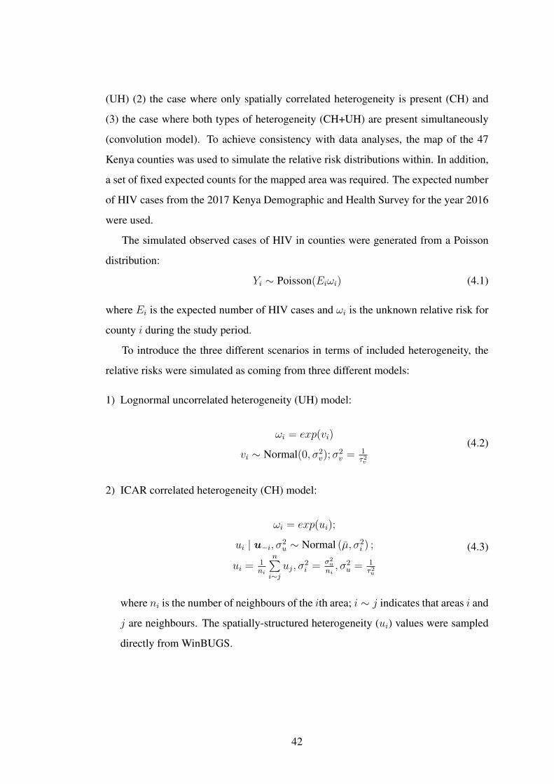
(UH) (2) the case where only spatially correlated heterogeneity is present (CH) and

(3) the case where both types of heterogeneity (CH+UH) are present simultaneously

(convolution model). To achieve consistency with data analyses, the map of the 47

Kenya counties was used to simulate the relative risk distributions within. In addition,

a set of fixed expected counts for the mapped area was required. The expected number

of HIV cases from the 2017 Kenya Demographic and Health Survey for the year 2016

were used.

The simulated observed cases of HIV in counties were generated from a Poisson

distribution:

Yi ∼ Poisson(Eiωi) (4.1)

where Ei is the expected number of HIV cases and ωi is the unknown relative risk for

county i during the study period.

To introduce the three different scenarios in terms of included heterogeneity, the

relative risks were simulated as coming from three different models:

1) Lognormal uncorrelated heterogeneity (UH) model:

ωi = exp(vi)

vi ∼ Normal(0, σ2v);σ

2v = 1

τ2v

(4.2)

2) ICAR correlated heterogeneity (CH) model:

ωi = exp(ui);

ui | u−i, σ2u ∼ Normal (µ, σ2

i ) ;

ui = 1ni

n∑i∼j

uj, σ2i = σ2

u

ni, σ2

u = 1τ2u

(4.3)

where ni is the number of neighbours of the ith area; i ∼ j indicates that areas i and

j are neighbours. The spatially-structured heterogeneity (ui) values were sampled

directly from WinBUGS.

42

3) Convolution (UH+CH) model:

ωi = exp(vi + ui);

vi ∼ Normal(0, σ2v);σ

2v = 1

τ2v;

ui | u−i, σ2u ∼ Normal (µ, σ2

i ) ;

ui = 1ni

n∑i∼j

uj, σ2i = σ2

u

ni, σ2

u = 1τ2u

(4.4)

Exactly the same values as simulated in (1) and (2) above were both included in

this model.

Data were simulated only for the case where the spatially-structured heterogeneity

was assumed to be largely present in the data while there was only a little uncorrelated

heterogeneity. This was achieved by setting τ 2v = 0.5 and τ 2

u = 5 (Neyens et al., 2012).

The observed counts data were simulated under these three models and then, re-

gardless of the sampling model, the 4 models described in Section 3.1 were fitted:

Poisson log-normal (PLN), Poisson log-skew normal (PLSN), Poisson log-t (PLT) and

Poisson log-skew- t (PLST) models. To improve on precision, 200 simulations were

run using the three scenarios above.

Model selection was done by using Mean Squared Error (MSE), defined as:

MSE =1

n− 1

n∑i=1

(ωi − ωi)2 (4.5)

where i = 1, ..., n with n = 47 which was averaged over the 200 simulated data sets.

The DIC goodness of fit measures were also compared for the simulated models.

Table 4.2 shows the MSE values obtained for the four analyzed models under the

three different scenarios.

Table 4.2: Simulation study: average MSE values (bold = lowest)

Analyzed lognormal ICAR Convolutionmodel (UH) (CH) (UH+CH)PLN 0.0145 0.0147 0.0142PLSN 00.0142 0.0141 0.0145PLT 0.0143 0.0139 0.0143PLST 0.0140 0.0145 0.0138

43

Although the results presented in Table 4.2 do not show large differences in average

MSE between models, they are consistent with the results seen in the analysis of real

data. For the case where uncorrelated heterogeneity (UH) is present (Lognormal and

Convolution columns), the Poisson log skew-t (PLST) model performs fairly well and

if only spatially correlated heterogeneity (CH) is present, Poisson log-t (PLT) model

performs well.

Table 4.3 show the DIC values obtained for the four analyzed models under the

three different scenarios.

Table 4.3: Simulation study: DIC values (bold = lowest)

Analyzed Lognormal ICAR Convolutionmodel (UH) (CH) (UH+CH)PLN 943.8 944.7 943.8PLSN 929.4 883.9 899.3PLT 920.9 897.6 869.7PLST 882.43 784.5 805.6

In terms of DIC, the PLST model is the best fitting model to the simulated data in

all the three scenarios of generating the relative risks. This agrees with the analysis of

the real HIV and AIDS data set presented in Section 4.1 above.

4.3 Application of Skew-t Spatial Combined Random Effects model to HIV andAIDS Data

In this section the skew spatial combined random effects model is used to analyze 2016

HIV and AIDS incidence data for n = 47 Kenya counties. The data has been described

in Section 1 of Chapter One. An overview of summary statistics is given in Table 4.4.

Table 4.4: Summary statistics for 2016 HIV and AIDS in Kenya

Statistic ValueMean 25689Variance 577357958Minimum 413Maximum 112226

Table 4.4 shows that the variance of the HIV and AIDS counts is very large, an

indication that there could be extra-Poisson variation in the data set. Standardizing

44

(Inskip et al., 1983) these observed counts for county population sizes and age dis-

tributions to provide the expected counts solves a part of the problem. It is also very

likely that part of the remaining variability can be explained by correlations through

space on one hand but also by spatially uncorrelated overdispersion (e.g., caused by

not standardizing for an important but still unknown factor) on the other hand.

In other words, estimates of the well-known Standardized Incidence Rates, SIRi =

Y i/Ei (Figure 4.2), may be overly simplistic and models which include random ef-

fects for both uncorrelated heterogeneity (UH) and correlated heterogeneity (CH) will

probably be better suited for these data.

Figure 4.2: Standardized incidence rates for 2016 HIV and AIDS in Kenya

The skew-t conditional autoregressive combined (STCARCOM) model proposed

in this thesis was compared to the existing classical disease mapping models: Poisson-

gamma (PG), Poisson-lognormal (PLN), intrinsic conditional autoregressive correlated

heterogeneity (ICAR CH ), convolution (CON), and the skew-t conditional autore-

gressive (STCAR) using the 2016 HIV and AIDS incidence data in n = 47 Kenya

counties.

Model estimation was carried out using Bayesian approach using the hierarchical

specification where all model parameters are assigned prior distributions. For the hy-

45

perparameters a and b in the gamma distribution of Poisson-gamma model, pCAR

combined model and STCAR combined model, a ∼ exp(1) and b ∼ Gamma(0.1, 1)

were used as suggested by Lawson et al. (2013). The prior distributions of the variance

parameters are 1/σ2v ∼Gamma(0.5, 0.0005) and 1/σ2

u ∼Gamma(0.5, 0.0005) Kelsall

and Wakefield (1999); a uniform prior distribution was used for the spatial smoothing

parameter ρ, that is, ρ ∼ U(0, 1) (Kelsall and Wakefield, 2002); the skewness para-

meter δ was given zero mean Gaussian distribution δ ∼ N(0, 0.01) (Branco and Dey,

2001) while the intercept term β0 was assigned a weakly informative Gaussian prior

distribution β0 ∼ N(0, 0.000001) (Arab, 2015); and finally the parameter k repres-

enting the degrees of freedom was assigned a truncated exponential prior distribution

p(k) ∝ λ0 expλ0k I {k > 2} with λ0 = 0.1 in order to favor heavy tails (Nathoo and

Ghosh, 2012).

Models were implemented using WinBUGS version 1.4 (Spiegelhalter et al., 2007;

Ntzoufras, 2011). For each model, 6,000 Markov chain Monte Carlo (MCMC) itera-

tions were ran, with the initial 2,000 discarded to cater for the burn-in and thereafter

keeping every tenth sample value. The 4,000 iterations left were used for assess-

ing convergence of the MCMC and parameter estimation. MCMC convergence were

monitored using trace plots, see Gelman et al. (2004). For model comparison and

goodness-of-fit (GOF), the deviance information criterion (DIC) proposed by (Spiegel-

halter et al., 2002) was adopted. The best fitting model is one with the smallest DIC

value. On the other hand, the overall loss across the data was assessed by the use of

the Mean Squared Predictive Error (MSPE). The best model for prediction is the one

with the lowest MSPE value.

The results are given in Table 4.5 below.

Table 4.5: Parameter estimates for the models

Model β0 σv σu ρ k δ pD DIC MSPEPG - 0.862 - - - - 47.01 636.51 51060PLN -0.055 0.8692 - - - - 75.30 693.13 50440ICAR CH -0.210 - 1.241 - - - 133.23 928.30 76130CON -0.225 0.240 1.218 - - - 67.05 676.60 50490STCAR 0.040 - 75.2 0.124 8.07 -0.370 6.04 595.77 50560STCARCOM 0.028 0.138 96.25 0.137 13.14 0.142 -103.04 487.10 50310

46

In terms of DIC, the models with the gamma overdispersion and skew-t random

effect terms are favored. It can be seen that the PG, STCAR and STCARCOM have

similar smaller DIC values as compared to the PLN, ICAR CH and CON models,

showing that the gamma- and skew-t random efffects improve the model fit as com-

pared to the normally distributed random effects. Considering the relative risk (RR)

estimates presented in Appendix 1, it is shown that the credibility intervals for RR

differ from 1 for all the counties. This indicates presence of important spatial hetero-

geneity in the data. It is noted here that the STCAR and STCARCOM models have the

smaller pD values, an evidence that these models are less parameterized as compared

to the other models. The proposed STCARCOM model has the smallest values for

both DIC and MSPE, indicating that this proposed model is the best in terms of model

fit and predictive behaviour. The respective WinBUGS code for this model is provided

in Appendix 3.

Similar conclusions are drawn from the parameter estimates, in which the estim-

ated values for the intercept β0, the standard deviations of the spatially-unstructured

and spatially-structured random effects σv and σu are shown. σv comes from either

the gamma distributed random effect in the PG and STCARCOM models or from the

log-normal distributed random effect in the PLN, ICAR CH and convolution models,

while σu comes from either the ICAR normal random effects in the ICAR CH and con-

volution models or the pCAR normal random effects in the STCAR and STCARCOM

models.

4.4 Simulation study for Skew-t Spatial Combined Random Effects Model

For the skew-t spatial combined random effects model analysis, the simulation proced-

ures presented in Section 4.2 for skew random effect models were also used. That is,

data were also simulated from a number of different possible relative risk models: (1)

the case where only uncorrelated heterogeneity is present (UH) (2) the case where only

spatially correlated heterogeneity is present (CH) and (3) the case where both types of

heterogeneity (CH+UH) are present simultaneously (convolution model). However,

in this case the three scenarios were simulated separately for two settings, setting

A where the data contained a large amount of uncorrelated heterogeneity and only

47

little spatially-structured heterogeneity on one hand and setting B where the spatially-

structured heterogeneity was largely present in the data while there was only little un-

correlated heterogeneity on the other. To simulate only a little relatively large amount

of UH (setting A), τ 2v = 0.05 was used while in the setting with little UH (setting B),

τ 2v = 0.5 was chosen (Neyens et al., 2012). Only a little amount of CH (setting A) was

simulated by setting τ 2u = 500 while a relatively high amount of CH (setting B) was

simulated by setting τ 2u = 5 (Neyens et al., 2012).

Again, 200 simulations of both settings A and B were run, separately, using the

three scenarios above. The simulated observed cases of HIV were analyzed with six

models: Poisson-gamma (PG), Poisson-lognormal (PLN), intrinsic conditional autore-

gressive correlated heterogeneity (ICAR CH ), convolution (CON), skew-t conditional

autoregressive (STCAR) and the skew-t conditional autoregressive combined (STCAR-

COM). The MSE was also used for model selection.

Table 4.6 show the MSE values obtained for the six models analyzed under the two

settings for the three different scenarios.

Table 4.6: Simulation study: average MSE values (bold = lowest) for setting A (large UH,small CH) and setting B (small UH, large CH)

Analyzed model

Setting A Setting BLog-normal ICAR Convolution Log-normal ICAR Convolution(UH) (CH) (UH+CH) (UH) (CH) (UH+CH)

PG 0.0140 0.0144 0.0142 0.0146 0.0140 0.0144PLN 0.0146 0.0149 0.0147 0.0145 0.0151 0.0147ICAR CH 0.0416 0.0433 0.0419 0.0418 0.0413 0.0419CON 0.0150 0.0153 0.0148 0.0148 0.0151 0.0146STCAR 0.0145 0.0147 0.0144 0.0137 0.0148 0.0145STCARCOM 0.0136 0.0142 0.0138 0.0145 0.0147 0.0143

The results presented in Table 4.6 do not show large differences in average MSE

between models, but are again consistent with the results obtained in the analysis of

real data: the skew-t spatial combined (STCARCOM) model behaves particularly well

when there is a large amount of uncorrelated heterogeneity (UH) present in the data

(setting A). In this setting, average MSE values are slightly lower for the STCAR-

COM for the case in which only UH was present in the data (Log-normal and Convo-

48

lution columns). This is also consistent with previous observations, which state that

the STCARCOM model does well when there is a large amount of overdispersion or

uncorrelated heterogeneity, but not necessarily when a map contains a lot of spatially

induced extra-variance (correlated heterogeneity).

Finally, Table 4.7 show the DIC values obtained for the six models analyzed under

the two settings for the three different scenarios.

Table 4.7: Simulation study: DIC values (bold = lowest) for setting A (large UH, small CH)and setting B (small UH, large CH)

Analyzed model

Setting A Setting BLog-normal ICAR Convolution Log-normal ICAR Convolution(UH) (CH) (UH+CH) (UH) (CH) (UH+CH)

PG 692.4 686.8 690.5 715.2 710.2 712.2PLN 855.6 803.4 840.5 778.5 874.5 902.4ICAR CH 927.2 932.4 929.6 930.1 926.3 928.7CON 746.5 743.5 740.4 754.7 743.8 748.3STCAR 701.3 711.3 702.6 725.5 720.6 717.1STCARCOM 670.8 652.6 675.7 662.8 687.4 673.5

In terms of DIC, the STCARCOM model is the best fitting model to the simulated

data in all the three scenarios of generating the relative risks under setting A. On the

other hand, when there is very little or zero extra-variance present in the data, the skew-

t spatial combined model, will analyze the data not as good as the normal distribution-

based solutions. This also confirms the results obtained in the analysis of real data in

which the skew-t spatial combined (STCARCOM) was the best fitting model.

4.5 Spatio-temporal Variation of HIV and AIDS Infection in Kenya

The parametric linear time trend and the non-parametric dynamic time trend models

were applied to to the HIV and AIDS data in Kenya for the period 2013-2016. The

models were implemented using Integrated Nested Laplace Approximation (INLA).

The corresponding R-INLA codes for spatio-temporal analysis of HIV and AIDS in

Kenya is provided in Appendix 4.

The spatial patterns for HIV and AIDS cases in Kenya for the period 2013-2016

are given in Figure 4.3.

49

Figure 4.3: The spatial pattern of HIV and AIDS incidence risks ζi = exp(ui) (a); Posteriorprobabilities P (ζi > 1|Y ) (b)

The left figure (a) presents the spatial incidence risk (ζi = exp(ui)) associated

to each county and constant along the period while the right figure (b) presents the

posterior probability that the spatial risk is greater than 1 (p = P (ζi > 1 | Y )).

Probabilities above 0.9 point towards high risk areas. Some discussions about refer-

ence thresholds in relative risks and cut-off probabilities can be obtained in Richardson

et al. (2004), Ugarte et al. (2009a) and Ugarte et al. (2009b). It is clear from this figure

that there is a higher risk of HIV and AIDS infection in the counties to the Western

region of Kenya as compared to the other counties. In particular, Homa Bay, Siaya,

Migori and Kisumu counties show high relative risks.

Figure 4.4 shows the posterior mean of the main time effect together with its 95%

credibility interval. This plot show a positive increment in the risk of HIV and AIDS

for every subsequent year.

50

Figure 4.4: Global linear temporal trend of HIV and AIDS incidence risks. Solid line: pos-terior mean for βt; Dashed lines: 95% credibility intervals

The temporal risk trend common to all counties are given in bottom figure in Figure

4.5 below.

51

Figure 4.5: Temporal trend of HIV and AIDS incidence risks

Generally, there is an increasing trend in the whole period which indicates that

there might be some factors affecting the whole country that produce an increase in

risk along the period. There is a non-linear trend behavior of the temporal pattern over

time, thus explaining the reason why the parametric linear trend models do not fit well

to the HIV and AIDS data as compared to the non-parametric ones.

The specific temporal trends (in log scale) for four selected counties are shown in

Figure 4.6.

52

Figure 4.6: Specific temporal trends for selected counties: Homa Bay, Bomet, Nairobi andWajir.

There is a clear differences among counties, which means including the interaction

term in the model is appropriate.

The spatio-temporal interactions for the HIV and AIDS are given in Figures 4.7-

4.10. It is clear from the information provided by the interaction maps that there is an

increase in risk as the maps are getting darker with years. A number of counties in the

Western region of Kenya show higher significant risk of HIV and AIDS as compared

to other regions.

53

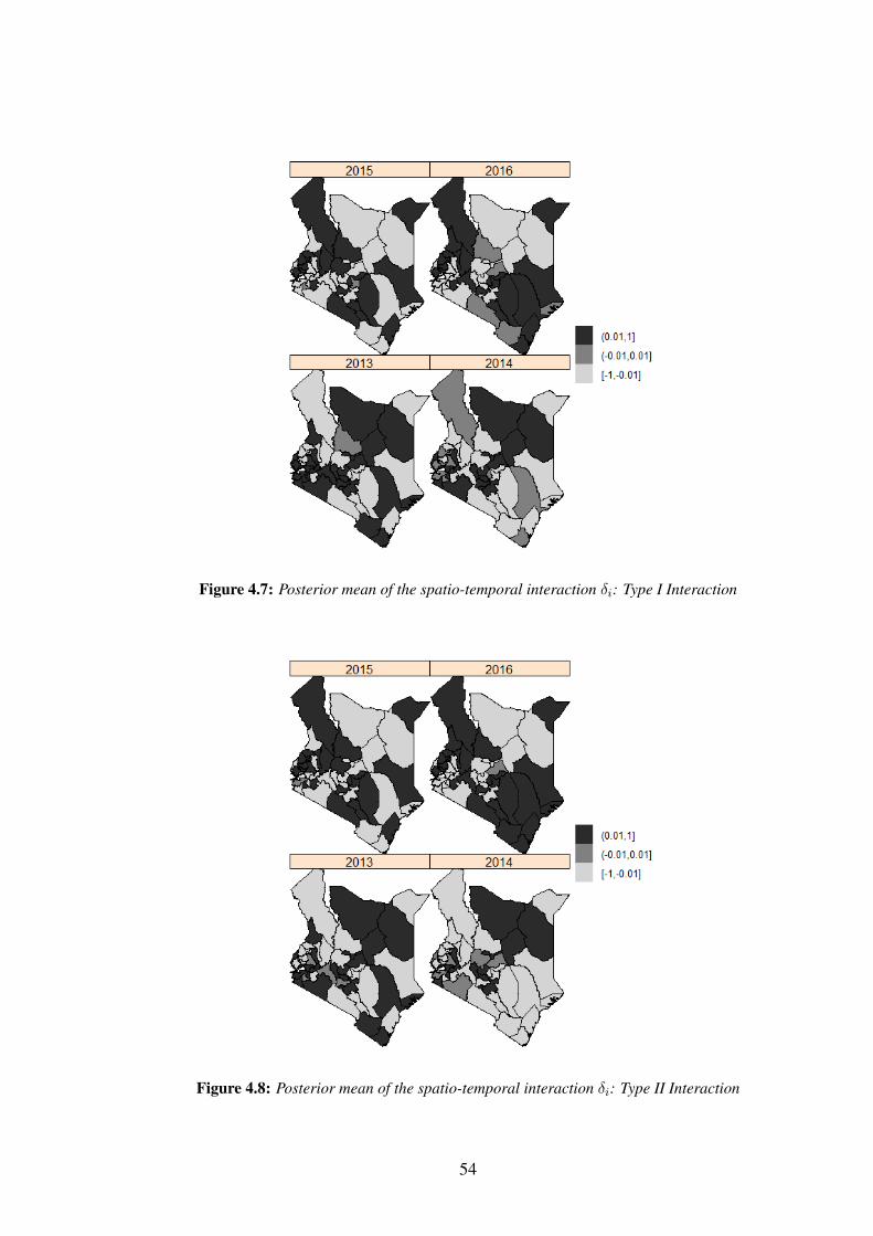
Figure 4.7: Posterior mean of the spatio-temporal interaction δi: Type I Interaction

Figure 4.8: Posterior mean of the spatio-temporal interaction δi: Type II Interaction

54

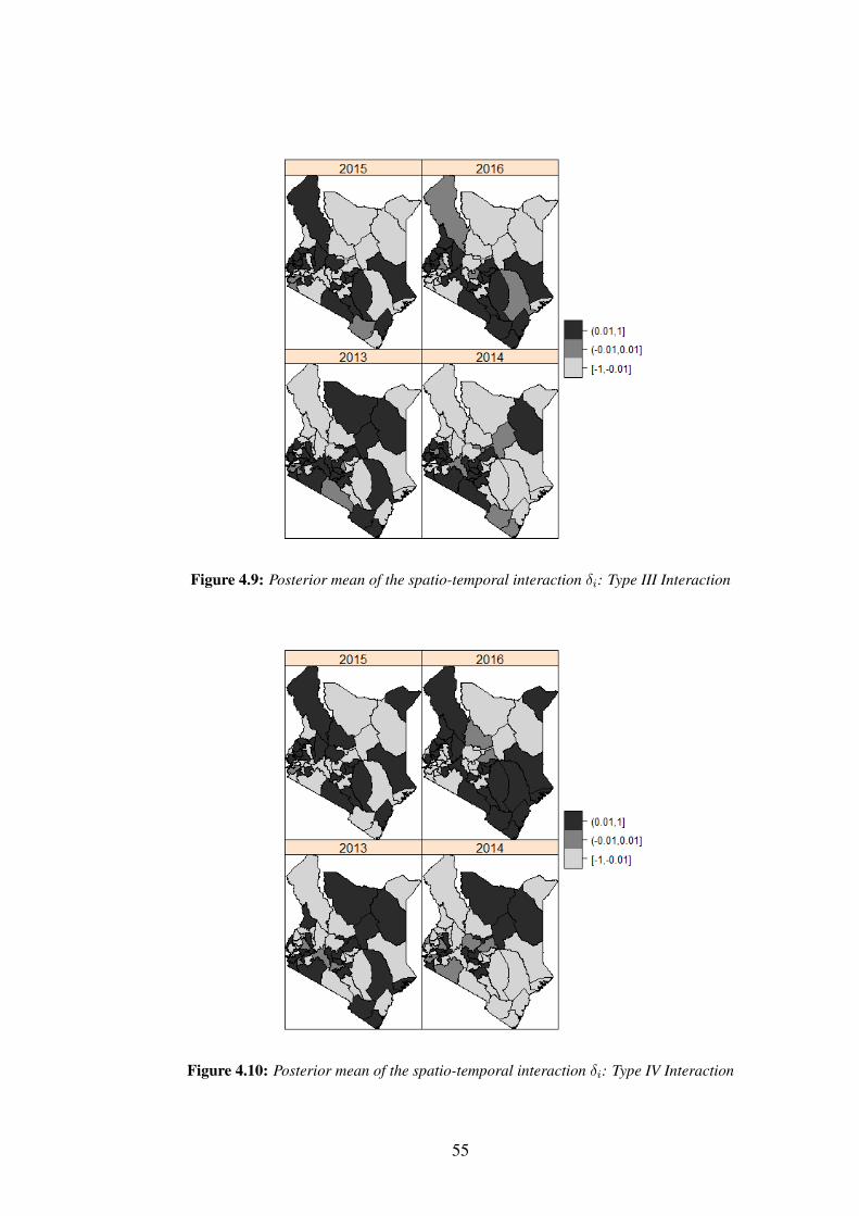
Figure 4.9: Posterior mean of the spatio-temporal interaction δi: Type III Interaction

Figure 4.10: Posterior mean of the spatio-temporal interaction δi: Type IV Interaction

55

CHAPTER FIVE

CONCLUSION AND RECOMMENDATIONS

5.1 Conclusion

Disease maps play a key role in descriptive spatial epidemiology. Maps are useful

for several purposes such as identification of areas with suspected elevations in risk,

formulation of hypotheses about disease aetiology, and assessing needs for health care

resource allocation.

A new model that relaxes the usual normality assumption on the spatially unstruc-

tured random effect by using the skew normal and skew-t distributions was introduced.

In the analysis of 2016 HIV and AID data in Kenya, it was found out that models whose

unstructured random effects follow skewed distributions generally perform better than

models with normally distributed unstructured random effects.

Another flexible model known as skew-t spatial combined random effects model

was also proposed. This new model combines a Poisson-gamma model with a spatially

structured skew-t random effect in the same model is presented. In the analysis of

2016 HIV and AID data in Kenya, the skew-t spatial combined model provided a

better alternative to the classical disease mapping models such as the popular Gaussian

spatial models, with improved modeling capabilities when the data contain a large

amount of uncorrelated heterogeneity. Simulation studies to assess the performance of

the skew random effect distribution models and the skew-t spatial combined random

effects model show that these proposed models perform better than the classical disease

mapping models.

Spatio-temporal models which include linear time trend, non-parametric and space-

time interactions models were also discussed. For modeling spatial random effect,

Leroux CAR (LCAR) prior was used and Bayesian analysis implemented using INLA.

INLA fit complex spatio-temporal models much faster than the Markov chain Monte

Carlo (MCMC) algorithm. INLA also has an additional advantage since it can be

easily implemented in the free software R using the package R-INLA. The INLA

methodology also offers several quantities such as the effective number of parameters

(pD) and the Deviance Information Criterion (DIC) for Bayesian model choice and

56

comparison.

Finally, the analysis of the 2013-206 Kenya HIV and AIDS data shows that counties

located in the Western region of Kenya show significantly higher risks as compared to

the other counties. In particular, Homa Bay, Siaya, Migori and Kisumu counties show

the highest risks. The reasons why these counties show high HIV and AIDS incidence

risks is still a subject that needs investigation and further research is required.

5.2 Recommendations for Further Research

Future work will consider extensions of the models presented in Chapter Three. For

example, the skew-t spatial combined model considered only explored the univariate

case. Future research will focus on the multivariate count data case, which is also

often encountered in many disease mapping problems. Furthermore, an extension of

the skew-t spatial combined model to the spatio-temporal setting can be of interest as

well. All the spatial and spatio-temporal models considered in this thesis are based

on single disease modeling. Further research can consider extending these models to

study multiple diseases. Finally, the models considered in this thesis were applied to

the analysis of HIV and AIDS data. Further research can consider the application of

these models to spatial and spatio-temporal analysis of other diseases as well.

57

REFERENCES

Abellan, J., Richardson, S. and Best, N. (2008). Use of space-time models to invest-

igate the stability of patterns of disease. Environmental Health Perspective, 116(8),

1111–1119.

Agresti, A. (2002). Categorical Data Analysis. Wiley, New Jersey, 2nd edition.

Arab, A. (2015). Spatial and spatio-temporal models for modeling epidemiological

data with excess zeros. International Journal of Environmental Resesearch & Public

Health, 12, 10536–10548.

Assuncao, R., Reis, I. and Oliveira, C. (2001). Diffusion and prediction of leish-

maniasis in a large metropolitan area in brazil with a bayesian space-time model.

Statistics in Medicine, 20, 2319–2335.

Azzalini, A. and Capitanio, A. (2003). Distributions generated by perturbation of

symmetry with emphasis on a multivariate skew-t distribution. Journal of the Royal

Statistical Society, Series B, 65, 367–389.

Banerjee, S., Carlin, B. P. and Gelfand, A. E. (2015). Hierarchical Modeling and

Analysis for Spatial Data. Chapman & Hal, London: CRC Press.

Bernardinelli, L., Clayton, D. and Montomoli, C. (1995). Bayesian estimates of disease

maps: How important are priors? Statistics in Medicine, 14, 2411–2431.

Besag, J., York, J. and Molli´e, A. (1991). Bayesian image restoration with two ap-

plications in spatial statistics (with discussion). Annals of the Institute of Statistical

Mathematics, 43, 1–59.

Best, N., Thomas, A., Waller, L., Conlon, E. and Arnold, R. (1999). Bayesian models

for spatially correlated disease and exposure data. In Bayesian Statistics 6, volume 6,

pages 131–156. Proceedings of the Sixth Valencia International Meeting, Oxford

University Press, USA.

58

Best, N., Richardson, S. and Thompson, A. (2005). A comparison of bayesian spatial

models for disease mapping. Statistical Methods of Medical Research, 14, 35–59.

Bithell, J. (2000). A classification of disease mapping methods. Statistics in Medicine,

19, 2203–2215.

Bivand, R. S., Gomez-Rubio, V. and Rue, H. (2015). Spatial data analysis with r-inla

with some extensions. Journal of Statistical Software, 63(20), 1–31.

Blangiardo, M. and Cameletti, M. (2015). Spatial and Spatio-Temporal Bayesian Mod-

els with R-INLA. John Wiley and Sons, Inc., New York.

Blangiardo, M., Cameletti, M., Baio, G. and Rue, H. (2013). Spatio-temporal bayesian

models with r-inla. Spatiotemporal Epidemiology, 4, 33–49.

Botella-Rocamora, P., Lopez-Quılez, A. and Martınez-Beneito, M. A. (2013). Spatial

moving average risk smoothing. Statistics in Medicine, 32, 2595–2612.

Box, G. and Tiao, G. (1973). Bayesian Inference in Statistical Analysis. Addison-

Wesley Pub. Co., UK.

Branco, M. and Dey, D. (2001). A general class of multivariate skew-elliptical distri-

butions. Journal of Multivariate Analysis, 79, 99–113.

Breslow, N. E. and Clayton, D. G. (1993). Approximate inference in generalized linear

mixed models. Journal of the American Statistical Association, 88, 9–25.

Casella, G. and George, E. I. (1992). Explaining the Gibbs sampler. The American

Statistician, 46, 167–174.

CBS and MOH (2004). Kenya Demographic & Health Survey 2003. Calverton,

Maryland: Central Bureau of Statistics (CBS) [Kenya], Ministry of Health (MOH)

[Kenya] and ORC Macro.

Chen, J., Zhang, D. and Davidian, M. (2002). A monte carlo em algorithm for gener-

alized linear mixed models with flexible random effects distribution. Biostatistics, 3

(3), 347–360.

59

Clayton, D. G. and Kaldor, J. (1987). Empirical bayes estimates of agestandardised

relative risks for use in disease mapping. Biometrics, 43, 671–691.

Coly, S., Garrido, M., Abrial, D. and Yao, A. F. (2019). Bayesian hierarchical models

for disease mapping applied to contagious pathologies. Biological Research.

Cressie, N. A. C. (1993). Statistics for Spatial Data. Wiley, CRC Press.

Dellaportas, P. and Roberts, G. O. (2003). An introduction to mcmc. In Spatial stat-

istics and computational methods (Aalborg, 2001), Volume 173 of Lecture Notes in

Statistics. Springer, New York.

Eberly, L. E. and Carlin, B. P. (2000). Identifiability and convergence issues for markov

chain monte carlo fitting of spatial models. Statistics in Medicine, 19(1718), 2279–

2294.

Elliott, P. and Wartenberg, D. (2004). Spatial epidemiology current approaches and

future challenges. Environmental Health Perspectives, 112, 998–1006.

Fong, Y., Rue, H. and Wakefield, J. (2010). Bayesian inference for generalized linear

mixed models. Biostatistics, 11, 397–412.

Gaetan, C. and Guyon, X. (2010). Spatial Statistics and Modeling, Series in Statistics.

Springer.

Gelfand, A., Diggle, P., Fuentes, M. and Guttorp, P. (2010). Handbook of Spatial

Statistics. Chapman & Hall/CRC, London.

Gelfand, A. and Ghosh, S. (1998). Model choice: A minimum posterior predictive loss

approach. Biometrika, 85, 1–11.

Gelfand, A. E. and Smith, A. F. M. (1990). Sampling-based approaches to calculating

marginal densities. Journal of the American Statistical Association, 85, 398–409.

Gelman, A., Carlin, J. B., Stern, H. S. and Rubin, D. (2004). Bayesian Data Analysis.

Chapman and Hall, London, 2nd edition.

60

Geman, S. and Geman, D. (1984). Stochastic relaxation, Gibbs distributions, and

the Bayesian restoration of images. IEEE Transactions on Pattern Analysis and

Machine Intelligence, 6, 721–741.

Genton, M. G. (2004). Skew-Elliptical Distributions and Their Applications: A Jour-

ney Beyond Normality. Chapman & Hall/CRC.

Gilks, W., Richardson, S. and Spiegelhalter, D. (1996). Markov chain Monte Carlo in

Practice. Boca Raton: Chapman & Hall/CRC.

Gilks, W., Richardson, S. and Spiegelhalter, D. (2005). Markov chain Monte Carlo.

Wiley, Hoboken.

Gilks, W. R., Clayton, D. G., Spiegelhalter, D. J., Best, N. G., McNeil, A. J., Sharples,

L. D. and Kirby, A. J. (1993). Modelling complexity: Applications of gibbs

sampling in medicine. Journal of the Royal Statistical Society, B 55, 39–52.

Gomez-Rubio, V., Bivand, R. S. and Rue, H. (2014). Spatial models using laplace

approximation methods. In Fischer, M. M. and Nijkamp, P. E., editors, Handbook

of Regional Science, pages 1401–1417. Springer, Berlin.

Green, P. J. and Richardson, S. (2002). Hidden markov models and disease mapping.

Journal of the American Statistical Association, 97, 1055–1070.

Held, L., Schrodle, B. and Rue, H. (2010). Posterior and cross-validatory predictive

checks: A comparison of mcmc and inla. In Kneib, T. and Tutz, G. (eds): Statistical

modelling and regression structures., pages 91–110. Heidelberg.

Hu, B., Ning, P., Li, Y., Xu, C., Christakos, G. and Wang, J. (2020). Space-time

disease mapping by combining bayesian maximum entropy and kalman filter: the

bme-kalman approach. International Journal of Geographical Information Science,

pages 1–24.

Inskip, H., Beral, V., Fraser, P. and Haskey, P. (1983). Methods for age-adjustments of

rates. Statistics in Medicine, 2, 483–93.

61

Kassahun, W., Neyens, T., Molenberghs, G., Faes, C. and Verbeke, G. (2012). Mod-

eling overdispersed longitudinal binary data using a combined beta and normal

random-effects model. Archives of Public Health, 70(7).

Kelsall, J. and Wakefield, J. (1999). Modelling spatial variation in disease risk; Tech-

nical Report. Imperial College, London.

Kelsall, J. and Wakefield, J. (2002). Modeling spatial variation in disease risk: a

geostatistical approach. Journal of the American Statistical Association, 97, 692–

701.

Kim, H. and Mallick, B. (2004). A bayesian prediction using the skew gaussian distri-

bution. Journal of Statistical Planning and Inference, 120, 85–101.

Kim, H., Sun, D. and Tsutakawa, R. K. (2002). Lognormal vs. gamma: Extra vari-

ations. Biometrika Journal, 44, 305–323.

KNBS (2010). Kenya Demographic & Health Survey 2008-09. Calverton, Maryland:

Kenya National Bureau of Statistics (KNBS) [Kenya] and ICF Macro.

KNBS, NASCOP, NACC, KEMRI and NCAPD (2015). Kenya Demographic & Health

Survey 2014. Rockville, MD, USA: Kenya National Bureau of Statistics, Ministry

of Health/Kenya, National AIDS Control Council/Kenya, Kenya Medical Research

Institute, National Council for Population and Development/Kenya, and ICF Inter-

national.

Knorr-Held, L. (2000). Bayesian modelling of inseparable space-time variation in

disease risk. Statistics in Medicine, 19(18), 2555–2567.

Knorr-Held, L. and Besag, J. (1998). Modelling risk from a disease in time and space.

Statistics in Medicine, 17(18), 2045–2060.

Lawson, A. and Lee, D. (2017). Bayesian disease mapping for public health. In

Handbook of Statistics, volume 36, pages 443–481. Elsevier.

Lawson, A. B. (2001). Tutorial in biostatistics: Disease map reconstruction. Statistics

in Medicine, 20, 2183–2203.

62

Lawson, A. B., Browne, W. J. and Vidal-Rodiero, C. L. (2009). Bayesian Disease

Mapping. Hierarchical Modeling in Spatial Epidemiology. Chapman and Hall/CRC

press, New York.

Lawson, A. B., Browne, W. J. and Vidal-Rodiero, C. L. (2013). Bayesian Disease

Mapping. Hierarchical Modeling in Spatial Epidemiology. Chapman and Hall/CRC

press, New York.

Lee, D. (2011). A comparison of conditional autoregressive models used in bayesian

disease mapping. Spatial and Spatio-temporal Epidemiology, 2(2), 79–89.

Leroux, B. G., Lei, X. and Breslow, N. (1999). Estimation of disease rates in small

areas: A new mixed model for spatial dependence. In Statistical models in epi-

demiology, the environment and clinical trials., pages 135–178, New York, 1999.

Springer-Verlag.

Lindgren, F. and Rue, H. (2015). Bayesian spatial modelling with r-inla. Journal of

Statistical Software, 63(1), 1–25.

MacNab, Y. C. (2003). Hierarchical bayesian modeling of spatially correlated health

service outcome and utilization rates. Biometrics, 59, 305–316.

MacNab, Y. C. (2007). Spline smoothing in bayesian disease mapping. Environmet-

rics, 18, 727–744.

MacNab, Y. C. (2011). On gaussian markov random fields and bayesian disease map-

ping. Statistical Methods in Medical Research, 20, 49–68.

MacNab, Y. C. (2014). On identification in bayesian disease mapping and ecological-

spatial regression models. Statistical Methods in Medical Research, 23(2), 134–155.

MacNab, Y. C. and Dean, C. B. (2000). Parametric bootstrap and penalized quasi-

likelihood inference in conditional autoregressive models. PubMed: 10960863, 19,

2421–2435.

MacNab, Y. C. and Dean, C. B. (2001). Autoregressive spatial smoothing and temporal

spline smoothing for mapping rates. Biometrics, 57, 949–956.

63

MacNab, Y. C. and Gustafson, P. (2007). Regression b-spline smoothing in bayesian

disease mapping: with an application to patient safety surveillance. Statistics in

Medicine, 26, 4455–4474.

Martino, S. and Rue, H. (2009). Implementing approximate Bayesian inference using

integrated nested Laplace approximation: A manual for the inla program. Depart-

ment of Mathematical Sciences, Norway.

Molenberghs, G., Verbeke, G. and Demetrio, G. (2007). An extended random-effects

approach to modeling repeated, overdispersed count data. Lifetime Data Anal, 13,

513–31.

Molenberghs, G., Verbeke, G., Demetrio, G. and Vieira, A. (2010). A family of gen-

eralized linear models for repeated measures with normal and conjugate random

effects. Stat Sci, 25, 325–47.

NASCOP (2009). Kenya AIDS Indicator Survey 2007: Final Report. National AIDS

and STI Control Programme, Nairobi, NASCOP.

NASCOP (2014). Kenya AIDS Indicator Survey 2012: Final Report. National AIDS

and STI Control Programme, Nairobi, NASCOP.

NASCOP, KNBS and MOH (2017). Kenya Demographic & Health Survey

2016. Rockville, MD, USA: Kenya National Bureau of Statistics, Ministry of

Health/Kenya, National AIDS Control Council/Kenya and ICF International.

Nathoo, F. S. and Ghosh, P. (2012). Skew-elliptical spatial random effect modeling for

areal data with application to mapping health utilization rates. Statistics in Medicine.

Neyens, T., Faes, C. and Molenberghs, G. (2012). A generalized poisson-gamma

model for spatially overdispersed data. Spatial and Spatio-temporal Epidemiology,

3, 185–194.

Ngesa, O., Achia, T. and Mwambi, H. (2014). A flexible random effects distribution

in disease mapping models. South African Statistical Journal, 48(1), 83–93.

64

Ntzoufras, I. (2011). Bayesian modeling using WinBUGS, volume 698. John Wiley &

Sons, Hoboken; New Jersey.

Palacios, M. (2006). Non-gaussian bayesian geostatistical modeling. Journal of the

American Statistical Association, 101, 604–618.

Rampaso, R., de Souza, A. D. P. and Flores, E. (2016). Bayesian analysis of spatial

data using different variance and neighbourhood structures. Journal of Statistical

Computation and Simulation, 86(3), 535–552.

R Core Team (2016). R: A language and environment for statistical computing. R

Foundation for Statistical Computing. MRC Biostatistics Unit, Austria.

Richardson, S. (2003). Spatialmodels in epidemiological applications. In Green, P.,

Hjort, N. and Richardson, S., editors, Highly Structured Stochastic Systems, pages

237–259. Oxford Statistical Science Series, UK.

Richardson, S., Thomson, A. and Best, N. a. (2004). Interpreting posterior relative risk

estimates in disease-mapping studies. Environ Health Pesp, 112, 1016–1025.

Riebler, A., Sørbye, S. H., Simpson, D. and Rue, H. (2016). An intuitive bayesian

spatial model for disease mapping that accounts for scaling. Statistical Methods in

Medical Research, 25(4), 1145–1165.

Robert, C. and Casella, G. (2005). Monte Carlo Statistical Methods. Springer, New

York, 2nd edition.

Rue, H. and Held, L. (2005). Gaussian Markov random fields: theory and applications.

CRC Press, London.

Rue, H. and Martino, S. (2007). Approximate bayesian inference for hierarchical gaus-

sian markov random field models. J Stat Plan Inference, 137, 3177–3192.

Rue, H., Martino, S. and Chopin, N. (2009). Approximate bayesian inference for latent

gaussian models by using integrated nested laplace approximations. Journal of the

Royal Statistical Society, Series B, 71, 319–392.

65

Sahu, S., Dey, D. and Branco, M. (2003). A new class of multivariate skew dis-

tributions with applications to bayesian regression models. Canadian Journal of

Statistics, 31, 129–150.

Schrodle, B. and Held, L. (2011a). A primer on disease mapping and ecological re-

gression using inla. Computation Stat, 26(2), 241–258.

Schrodle, B. and Held, L. (2011b). Spatio-temporal disease mapping using inla. En-

vironmetrics, 22, 725–734.

Schrodle, B., Held, L. and Riebler, A. (2011). Using integrated nested laplace ap-

proximations for the evaluation of veterinary surveillance data from switzerland: a

case-study. Journal of the Royal Statistical Society, Series C, 60, 261–279.

Sherman, M. (2011). Spatial Statistics and Spatio-Temporal Data: Covariance Func-

tions and Directional Properties. Wiley, UK.

Spiegelhalter, D., Best, N., Carlin, B. and van der Linde, A. (2002). Bayesian meas-

ures of model complexity and fit (with discussion). Journal of the Royal Statistical

Society: Series B (Statistical Methodology), 64(4), 583–639.

Spiegelhalter, D., Thomas, A., Best, N. and Lunn, D. (2007). WinBUGS User Manual,

Version 1.4.3. MRC Biostatistics Unit, UK.

Tierney, L. and Kadane, J. B. (1986). Accurate approximations fo posterior moments

and marginal densities. J Am Stat Assoc, 81, 82–86.

Ugarte, M. D., Adin, A., Goicoa, T. and Militino, A. F. (2014). On fitting spatiotem-

poral disease mapping models using approximate bayesian inference. Stat Methods

Med Res, 23(6), 507–530.

Ugarte, M. D., Adin, A., Goicoa, T. and Militino, A. F. (2017). One-dimensional, two-

dimensional, and three dimensional b-splines to specify space–time interactions in

bayesian disease mapping: Model fitting and model identifiability. Spatial Statistics,

22, 451–468.

66

Ugarte, M. D., Goicoa, T. and Etxeberrı´a, J. (2012a). A p-spline anova type model in

space-time disease mapping. Stoch Env Res Risk A, 26, 835–845.

Ugarte, M. D., Goicoa, T. and Etxeberrı´a, J. (2012b). Projections of cancer mortality

risks using spatio-temporal p–spline models. Stat Methods Med Res, 21, 545–560.

Ugarte, M. D., Goicoa, T. and Ibanez, B. et al. (2009a). Evaluating the performance of

spatio-temporal bayesian models in disease mapping. Environmetrics, 20, 647–665.

Ugarte, M. D., Goicoa, T. and Militino, A. F. (2009b). Empirical bayes and fully bayes

procedures to detect high risk areas in disease mapping. Comput Stat Data Anal, 53,

2938–2949.

Ugarte, M. D., Goicoa, T. and Militino, A. F. (2010). Spatio-temporal modeling of

mortality risks using penalized splines. Environmetrics, 21, 270–289.

Wakefield, J. (2007). Disease mapping and spatial regression with count data. Biostat-

istics, 8(2), 158–183.

Waller, L. A. and Gotway, C. A. (2004). Applied Spatial Statistics for Public Health

Data, volume 368. John Wiley & Sons, Hoboken, New Jersey.

Wolpert, R. and Ickstadt, K. (1998). Poisson gamma random field models for spatial

statistics. Biometrika, 85, 251–67.

67

APPENDICES

Appendix 1: RR estimates for the 2016 HIV and AIDS in Kenya

PG PLN CON pCARCOM STCAR STCARCOM node mean sd mean sd mean sd mean sd mean sd mean sd

RR[1] 0.9549 0.0098 0.9547 0.0099 0.9547 0.0099 0.9544 0.01 0.9543 0.0097 0.9545 0.01 RR[2] 0.2971 0.0038 0.2972 0.0038 0.2971 0.0039 0.2971 0.0039 0.2972 0.0038 0.2971 0.0039 RR[3] 0.0897 0.0044 0.0895 0.0044 0.0894 0.0044 0.0896 0.0044 0.0898 0.0044 0.0898 0.0044 RR[4] 0.0525 0.0016 0.0525 0.0016 0.0526 0.0017 0.0526 0.0016 0.0526 0.0016 0.0525 0.0016 RR[5] 0.3627 0.0043 0.3626 0.0043 0.3629 0.0044 0.3626 0.0043 0.3627 0.0043 0.3627 0.0044 RR[6] 0.5176 0.0044 0.5178 0.0044 0.5177 0.0043 0.5178 0.0044 0.5178 0.0043 0.5179 0.0043 RR[7] 0.7821 0.005 0.7821 0.0049 0.7819 0.0049 0.7821 0.0049 0.7821 0.0047 0.7822 0.005 RR[8] 0.3889 0.0043 0.389 0.0044 0.3889 0.0043 0.389 0.0042 0.3891 0.0043 0.3889 0.0044 RR[9] 0.4654 0.0019 0.4654 0.0019 0.4653 0.0019 0.4654 0.0019 0.4654 0.0019 0.4654 0.0018 RR[10] 1.243 0.0055 1.243 0.0054 1.243 0.0055 1.243 0.0053 1.243 0.0053 1.243 0.0053 RR[11] 0.6203 0.0051 0.6203 0.0051 0.6205 0.0051 0.6205 0.0051 0.6206 0.0052 0.6205 0.0051 RR[12] 0.1114 0.002 0.1114 0.0019 0.1114 0.002 0.1115 0.0019 0.1116 0.002 0.1115 0.0019 RR[13] 1.127 0.0136 1.127 0.0134 1.127 0.0135 1.128 0.0137 1.127 0.0137 1.128 0.0139 RR[14] 0.8873 0.0105 0.8872 0.0104 0.8873 0.0104 0.8871 0.0104 0.8876 0.0104 0.8872 0.0102 RR[15] 0.7778 0.0041 0.778 0.0041 0.7779 0.0042 0.7778 0.0041 0.7777 0.0042 0.7779 0.0043 RR[16] 1.494 0.0152 1.494 0.0152 1.495 0.0147 1.494 0.0152 1.494 0.0152 1.494 0.0154 RR[17] 0.5964 0.0031 0.5964 0.0031 0.5965 0.0031 0.5965 0.0032 0.5965 0.0031 0.5965 0.003 RR[18] 0.5834 0.0043 0.5834 0.0044 0.5833 0.0043 0.5833 0.0043 0.5834 0.0042 0.5833 0.0043 RR[19] 5.259 0.0155 5.259 0.0157 5.259 0.0157 5.259 0.0157 5.259 0.0155 5.26 0.0157 RR[20] 0.9854 0.0056 0.9855 0.0056 0.9854 0.0054 0.9854 0.0055 0.9854 0.0054 0.9853 0.0055 RR[21] 1.057 0.0098 1.057 0.0098 1.057 0.01 1.057 0.0098 1.057 0.0098 1.057 0.0099 RR[22] 0.8498 0.009 0.8497 0.009 0.8501 0.0089 0.8495 0.009 0.8501 0.0088 0.85 0.009 RR[23] 0.7996 0.0049 0.7995 0.005 0.7996 0.0049 0.7997 0.0049 0.7996 0.0049 0.7997 0.0049 RR[24] 0.8279 0.0065 0.828 0.0065 0.828 0.0066 0.8281 0.0066 0.8282 0.0066 0.8281 0.0067 RR[25] 4.219 0.0143 4.219 0.0145 4.219 0.0142 4.219 0.014 4.219 0.014 4.219 0.014 RR[26] 0.7385 0.0063 0.7386 0.0062 0.7387 0.0062 0.7384 0.0065 0.7383 0.0062 0.7386 0.0063 RR[27] 0.3976 0.0061 0.3974 0.006 0.3977 0.0061 0.3977 0.0061 0.3977 0.0061 0.3975 0.006 RR[28] 1.116 0.0058 1.116 0.0058 1.116 0.0059 1.116 0.0057 1.116 0.0057 1.116 0.0058 RR[29] 0.6708 0.0049 0.6707 0.0049 0.6707 0.0048 0.6708 0.0048 0.6708 0.0049 0.6708 0.0048 RR[30] 0.686 0.0033 0.686 0.0033 0.686 0.0033 0.6861 0.0032 0.6861 0.0033 0.6861 0.0031 RR[31] 5.53 0.0215 5.53 0.0219 5.529 0.0218 5.53 0.0217 5.529 0.0213 5.529 0.0219 RR[32] 0.5923 0.0058 0.5921 0.0058 0.5921 0.0059 0.592 0.006 0.592 0.0058 0.592 0.0058 RR[33] 1.366 0.01 1.365 0.0098 1.365 0.0098 1.365 0.0101 1.366 0.0099 1.365 0.0098 RR[34] 0.7317 0.0051 0.7319 0.0051 0.7318 0.0051 0.732 0.005 0.7323 0.005 0.7319 0.0051 RR[35] 0.9897 0.0064 0.9897 0.0063 0.9897 0.0064 0.9897 0.0065 0.9897 0.0063 0.9897 0.0061 RR[36] 0.9003 0.0052 0.9001 0.0052 0.9002 0.0052 0.9002 0.0052 0.9002 0.0052 0.9 0.0052 RR[37] 3.032 0.0111 3.033 0.0108 3.032 0.0109 3.032 0.0111 3.033 0.011 3.032 0.0111 RR[38] 1.202 0.02 1.202 0.0204 1.201 0.0204 1.201 0.0201 1.202 0.0205 1.202 0.0207 RR[39] 0.9307 0.0051 0.9308 0.005 0.9308 0.0051 0.9306 0.0051 0.9308 0.0051 0.9308 0.0051 RR[40] 1.114 0.007 1.114 0.0071 1.114 0.007 1.114 0.007 1.114 0.0071 1.114 0.007 RR[41] 1.206 0.0088 1.206 0.009 1.206 0.0089 1.206 0.009 1.206 0.009 1.206 0.0091 RR[42] 1.042 0.0074 1.042 0.0073 1.042 0.0073 1.042 0.0072 1.042 0.0074 1.042 0.0073 RR[43] 0.7122 0.0085 0.7123 0.0085 0.7126 0.0087 0.7123 0.0086 0.7124 0.0085 0.7121 0.0083 RR[44] 0.9263 0.0076 0.9263 0.0076 0.9264 0.0076 0.9263 0.0077 0.9265 0.0076 0.9263 0.0077 RR[45] 1.284 0.009 1.285 0.0089 1.285 0.0092 1.285 0.0091 1.285 0.0093 1.284 0.009 RR[46] 1.204 0.0048 1.204 0.0048 1.204 0.0048 1.204 0.0049 1.204 0.0049 1.204 0.0048 RR[47] 1.357 0.0083 1.357 0.0084 1.357 0.0083 1.357 0.0085 1.357 0.0083 1.357 0.0084

68

Appendix 2: WinBugs code for Skew-t Model

# Model

model {

# Likelihood

for (i in 1 : N) {

y[i] ˜ dpois(mu[i])

log(mu[i]) <- log(E[i]) + beta0 + phi[i]

RR[i] <- exp(beta0+phi[i]) # Area-specific relative risk

phi[i]<-sqrt(1/eta[i])*(delta*abs(Z[i])+ v[i])

v[i]˜dnorm(0,tau)

# skew variables:

eta[i]˜dgamma(df,df)

Z[i]˜dnorm(0,1)

smr[i] <- (y[i])/(E[i])

ypred[i] ˜dpois(mu[i])

PPL[i] <- pow(ypred[i]-y[i],2)

}

mspe <- mean(PPL[])

# Other priors:

beta0 ˜dnorm(0,1.0E-6)

tau ˜ dgamma(0.5, 0.0005) # prior on precision

variance<- 1/tau # variance

sigma <- sqrt(1 / tau) # standard deviation

df<-k/2

k˜dexp(lambda.nu)I(2,)

lambda.nu<- 0.1

delta ˜dnorm(0, 0.01)

}

# Data

# Initials

69

list(beta0=0, tau=1, k=2, delta= -1,

v=c(0,0,0,0,0,0,0,0,0,0,0,0,0,0,0,0,0,0,0,0,

0,0,0,0,0,0,0,0,0,0,0,0,0,0,0,0,0,0,0,0,0,0,0,0,0,0,0),

Z=c(0,0,0,0,0,0,0,0,0,0,0,0,0,0,0,0,0,0,0,0,0,0,0,0,0,0,0,0,0,0,

0,0,0,0,0,0,0,0,0,0,0,0,0,0,0,0,0),

eta=c(1,1,1,1,1,1,1,1,1,1,1,1,1,1,1,1,1,1,1,1,1,1,1,1,1,1,1,1,1,1,

1,1,1,1,1,1,1,1,1,1,1,1,1,1,1,1,1),

ypred=c(1,1,1,1,1,1,1,1,1,1,1,1,1,1,1,1,1,1,1,1,1,1,1,1,1,1,1,1,1,1,

1,1,1,1,1,1,1,1,1,1,1,1,1,1,1,1,1))

70

Appendix 3: WinBugs code for Skew-t Spatial Combined Random Effects Model

#Model

model{

#Likelihood

for (i in 1 :N) {

# Specifying the likelihood:

y[i] ˜ dpois(mu[i])

log(mu[i])<-log(E[i])+log(theta[i])+beta0+phi[i]

RR[i] <- theta[i]*exp(beta0+phi[i]) # Area-specific relative risk

phi[i]<-(U[i])/(sqrt(eta[i]))

omega.U[i]<- delta*abs(Z[i])

M[i]<-1/E[i]

smr[i] <- (y[i])/(E[i])

ypred[i] ˜dpois(mu[i])

PPL[i] <- pow(ypred[i]-y[i],2)

# skew variables:

eta[i]˜dgamma(df,df)

Z[i]˜dnorm(0,1)

# Overdispersion random effect:

theta[i] ˜ dgamma(a,b)

}

cumsum[1] <- 0

for(i in 2:(N+1)) {

cumsum[i] <- sum(num[1:(i-1)])

}

for(k in 1 : sumNumNeigh) {

for(i in 1:N) {

pick[k,i] <- step(k - cumsum[i] - epsilon) * step(cumsum[i+1] - k)

# pick[k,i] = 1 if cumsum[i] < k <= cumsum[i=1]; otherwise, pick[k,i] = 0

}

71

C[k] <- sqrt(E[adj[k]] / inprod(E[], pick[k,])) # weight for each pair of neighbours

}

epsilon <- 0.0001

mspe <- mean(PPL[])

# Proper CAR prior distribution for spatial random effects:

U[1:N] ˜ car.proper(omega.U[], C[],adj[], num[], M[], prec, rho)

# Other priors:

beta0 ˜dnorm(0,1.0E-6)

a˜dexp(1)

b˜dgamma(0.1,1)

prec˜ dgamma(0.5, 0.0005)

sigma<- sqrt(1 / prec)

df<-K/2

K˜dexp(lambda.nu)I(2,)

lambda.nu<- 0.1

delta ˜dnorm(0, 0.01)

#gamma˜dbeta(18,2)I(,0.99)

rho.min <- min.bound(C[], adj[], num[], M[])

rho.max <- max.bound(C[], adj[], num[], M[])

rho ˜ dunif(rho.min, rho.max)

}

# Data

# Initials

list(beta0=0, a=1, b=1, prec = 1, K=2, delta= -1, rho=0.1,

U=c(0,0,0,0,0,0,0,0,0,0,0,0,0,0,0,0,0,0,0,0,0,0,0,0,0,0,0,0,0,0,

0,0,0,0,0,0,0,0,0,0,0,0,0,0,0,0,0),

theta=c(0.5, 1.5, 0.3, 0.7, 2.5, 1.3, 0.5, 0.4, 0.3, 2.1, 3, 2.3, 0.6, 2.8, 0.4, 0.5, 0.2, 2.4, 0.3, 2.6, 0.3, 1.5, 0.5, 0.4, 0.7, 1.5, 0.9, 5.2, 0.5, 0.4, 0.2, 0.8, 2.1,

0.4, 0.2, 0.3, 0.2, 0.3, 0.2, 1.2, 0.2, 0.6, 1.6, 1, 0.2, 0.8, 0.7),

Z=c(0,0,0,0,0,0,0,0,0,0,0,0,0,0,0,0,0,0,0,0,0,0,0,0,0,0,0,0,0,0,

0,0,0,0,0,0,0,0,0,0,0,0,0,0,0,0,0),

eta=c(1,1,1,1,1,1,1,1,1,1,1,1,1,1,1,1,1,1,1,1,1,1,1,1,1,1,1,1,1,1,

72

1,1,1,1,1,1,1,1,1,1,1,1,1,1,1,1,1),

ypred=c(1,1,1,1,1,1,1,1,1,1,1,1,1,1,1,1,1,1,1,1,1,1,1,1,1,1,1,1,1,1,

1,1,1,1,1,1,1,1,1,1,1,1,1,1,1,1,1))

73

Appendix 4: R-INLA codes for Spatio-temporal Analysis of HIV and AIDS inKenya

require(INLA)

inla.setOption(scale.model.default=FALSE)

require(splancs)

require(sp)

require(fields)

require(maptools)

require(lattice)

require(abind)

library(spdep)

data <- read.csv(paste(" ",sep=""))

kenya <- readShapePoly(paste("",sep=""))

S=47

T=4

y.vector <- as.vector(as.matrix(data[,2:5]))#by column

E.vector <- as.vector(as.matrix(data[,6:9]))#by column

year <- numeric(0)

for(i in 1:4){

year<- append(year,rep(i,dim(data)[1]))}

county <- as.factor(rep(data[,1],4))

data <- data.frame(y= y.vector, E=E.vector,

ID.area=as.numeric(county),ID.area1=as.numeric(county),

year=year,ID.year = year, ID.year1=year,

ID.area.year = seq(1,length(county)))

temp <- poly2nb(kenya)

nb2INLA("kenya.graph", temp)

Kenya.adj <- paste("",sep="")

H <- inla.read.graph(filename="kenya.graph")

# Temporal graph

D1 <- diff(diag(T),differences=1)

74

Q.gammaRW1 <- t(D1)%*%D1

D2 <- diff(diag(T),differences=2)

Q.gammaRW2 <- t(D2)%*%D2

Q.xi <- matrix(0, H$n, H$n)

for (i in 1:H$n){

Q.xi[i,i]=H$nnbs[[i]]

Q.xi[i,H$nbs[[i]]]=-1}

Q.Leroux <- diag(S)-Q.xi

names <- kenya$NAME

data.kenya <- attr(kenya, "data")

formula.ST1 <- y ˜ f(ID.area,model="bym",graph=Kenya.adj) +

f(ID.year,model="rw2") + f(ID.year1,model="iid")

model.ST1 <- inla(formula.ST1,family="poisson",data=data,E=E,

control.predictor=list(compute=TRUE))

temporal.CAR <- lapply(model.ST1$marginals.random$ID.year,

function(X){marg <- inla.tmarginal(function(x) exp(x), X)

inla.emarginal(mean, marg)})

temporal.IID <- lapply(model.ST1$marginals.random$ID.year1,

function(X){marg <- inla.tmarginal(function(x) exp(x), X)

inla.emarginal(mean, marg)})

###########################

### Spacetime interactions

###########################

#Type I interaction and RW2 prior for time#

formula.intI <- y ˜ f(ID.area, model="generic1",

Cmatrix= Q.Leroux, constr=TRUE,

hyper=list(prec=list(prior="loggamma", param=c(1,0.01)),

beta=list(prior="logitbeta", param=c(4,2))))+f(ID.year1,

model="iid", constr=TRUE,hyper=list(prec=list(prior="loggamma",

param=c(1,0.01))))+f(ID.year, model="rw2", constr=TRUE,

hyper=list(prec=list(prior="loggamma", param=c(1,0.00005))))+

75

f(ID.area.year, model="iid", constr=TRUE,

hyper=list(prec=list(prior="loggamma", param=c(1,0.00005))),

extraconstr=list(A=matrix(rep(1:T,S),1,S*T),e=0))

model.intI<-inla(formula.intI, family="poisson", data=data, E=E,

control.predictor=list(compute=TRUE,cdf=c(log(1))),

control.compute=list(dic=TRUE),

control.inla=list(strategy="laplace"))

#Type II interaction and RW2 prior for time #

R <- kronecker(Q.gammaRW2,diag(S))

r.def <- 2*S

A.constr <- kronecker(matrix(1,1,T),diag(S))

formula.intII <- y ˜ f(ID.area, model="generic1",

Cmatrix= Q.Leroux, constr=TRUE,

hyper=list(prec=list(prior="loggamma", param=c(1,0.01)),

beta=list(prior="logitbeta", param=c(4,2))))+f(ID.year1,

model="iid",constr=TRUE,hyper=list(prec=list(prior="loggamma",

param=c(1,0.01))))+f(ID.year, model="rw2", constr=TRUE,

hyper=list(prec=list(prior="loggamma", param=c(1,0.00005))))+

f(ID.area.year,model="generic0", Cmatrix=R, constr=TRUE,

hyper=list(prec=list(prior="loggamma", param=c(1,0.00005))),

extraconstr=list(A=A.constr, e=rep(0,S)))

model.intII<-inla(formula.intII, family="poisson", data=data, E=E,

control.predictor=list(compute=TRUE,cdf=c(log(1))),

control.compute=list(dic=TRUE),

control.inla=list(strategy="laplace"))

# Type III interaction and RW2 prior for time#

R <- kronecker(diag(T),Q.xi)

r.def <- T

A.constr <- kronecker(diag(T),matrix(1,1,S))

formula.intIII <- y ˜ f(ID.area, model="generic1",

76

Cmatrix= Q.Leroux, constr=TRUE,

hyper=list(prec=list(prior="loggamma", param=c(1,0.01)),

beta=list(prior="logitbeta", param=c(4,2))))+f(ID.year1,

model="iid", constr=TRUE,hyper=list(prec=list(prior="loggamma",

param=c(1,0.01))))+f(ID.year, model="rw2", constr=TRUE,

hyper=list(prec=list(prior="loggamma",

param=c(1,0.00005))))+f(ID.area.year, model="generic0",

Cmatrix=R, rankdef=r.def,constr=TRUE,

hyper=list(prec=list(prior="loggamma", param=c(1,0.00005))),

extraconstr=list(A=A.constr, e=rep(0,T)))

model.intIII<-inla(formula.intIII, family="poisson", data=data,

E=E,control.predictor=list(compute=TRUE,cdf=c(log(1))),

control.compute=list(dic=TRUE),

control.inla=list(strategy="laplace"))

#Type IV interaction and RW2 prior for time #

R <- kronecker(Q.gammaRW2,Q.xi)

r.def <- 2*S+T-2

A1 <- kronecker(matrix(1,1,T),diag(S))

A2 <- kronecker(diag(T),matrix(1,1,S))

A.constr <- rbind(A1,A2)

formula.intIV <- y ˜ f(ID.area, model="generic1",

Cmatrix= Q.Leroux, constr=TRUE,

hyper=list(prec=list(prior="loggamma",param=c(1,0.01)),

beta=list(prior="logitbeta",param=c(4,2))))+

f(ID.year1, model="iid", constr=TRUE,

hyper=list(prec=list(prior="loggamma", param=c(1,0.01))))+

f(ID.year, model="rw2", constr=TRUE,

hyper=list(prec=list(prior="loggamma", param=c(1,0.00005))))+

f(ID.area.year, model="generic0", Cmatrix=R, rankdef=r.def,

constr=TRUE, hyper=list(prec=list(prior="loggamma",

param=c(1,0.00005))),extraconstr=list(A=A.constr, e=rep(0,S+T)))

77

model.intIV<-inla(formula.intIV, family="poisson", data=data, E=E,

control.predictor=list(compute=TRUE,cdf=c(log(1))),

control.compute=list(dic=TRUE),

control.inla=list(strategy="laplace"))

delta.intI <- data.frame(delta=model.intI$summary.random$

ID.area.year[,2],year=data$ID.year,ID.area=data$ID.area)

delta.intI.matrix <- matrix(delta.intI[,1], 47,4,byrow=FALSE)

rownames(delta.intI.matrix)<- delta.intI[1:47,3]

delta.intII <- data.frame(delta=model.intII$summary.random$

ID.area.year[,2],year=data$ID.year,ID.area=data$ID.area)

delta.intII.matrix <- matrix(delta.intII[,1], 47,4,byrow=FALSE)

rownames(delta.intII.matrix)<- delta.intII[1:47,3]

delta.intIII <- data.frame(delta=model.intIII$summary.random$

ID.area.year[,2],year=data$ID.year,ID.area=data$ID.area)

delta.intIII.matrix <- matrix(delta.intIII[,1], 47,4,byrow=FALSE)

rownames(delta.intIII.matrix)<- delta.intIII[1:47,3]

delta.intIV <- data.frame(delta=model.intIV$summary.random$

ID.area.year[,2],year=data$ID.year,ID.area=data$ID.area)

delta.intIV.matrix <- matrix(delta.intIV[,1], 47,4,byrow=FALSE)

rownames(delta.intIV.matrix)<- delta.intIV[1:47,3]

# Check the absence of spatial trend for (intI)

cutoff.interaction <- c(-1,-0.01,0.01,1)

delta.intI.factor <- data.frame(NAME=data.kenya$NAME)

for(i in 1:4){delta.factor.temp <- cut(delta.intI.matrix[,i],

breaks=cutoff.interaction,include.lowest=TRUE)

delta.intI.factor <- cbind(delta.intI.factor,delta.factor.temp)}

colnames(delta.intI.factor)<- c("NAME",seq(2013,2016))

# Check the absence of spatial trend for (intII)

delta.intII.factor <- data.frame(NAME=data.kenya$NAME)

for(i in 1:4){delta.factor.temp <- cut(delta.intII.matrix[,i],

78

breaks=cutoff.interaction,include.lowest=TRUE)

delta.intII.factor <- cbind(delta.intII.factor,delta.factor.temp)}

colnames(delta.intII.factor)<- c("NAME",seq(2013,2016))

# Check the absence of spatial trend (intIII)

delta.intIII.factor <- data.frame(NAME=data.kenya$NAME)

for(i in 1:4){delta.factor.temp <- cut(delta.intIII.matrix[,i],

breaks=cutoff.interaction,include.lowest=TRUE)

delta.intIII.factor <- cbind(delta.intIII.factor,delta.factor.temp)}

colnames(delta.intIII.factor)<- c("NAME",seq(2013,2016))

# Check the absence of Spatial trend (intIV)

delta.intIV.factor <- data.frame(NAME=data.kenya$NAME)

for(i in 1:4){delta.factor.temp <- cut(delta.intIV.matrix[,i],

breaks=cutoff.interaction,include.lowest=TRUE)

delta.intIV.factor <- cbind(delta.intIV.factor,delta.factor.temp)}

colnames(delta.intIV.factor)<- c("NAME",seq(2013,2016))

#################################################

# Spatio-temporal interaction: Type I Interaction

#################################################

attr(kenya, "data") <- data.frame(data.kenya,

intI=delta.intI.factor, intII=delta.intII.factor,

intIII=delta.intIII.factor,intIV=delta.intIV.factor)

trellis.par.set(axis.line=list(col=NA))

spplot(obj=kenya, zcol=c("intI.2013","intI.2014","intI.2015",

"intI.2016"), col.regions=gray(2.5:0.5/3),

names.attr=seq(2013,2016),main="")

###################################################

# Spatio-temporal interaction: Type II Interaction

###################################################

spplot(obj=kenya, zcol=c("intII.2013","intII.2014","intII.2015",

79

"intII.2016"), col.regions=gray(2.5:0.5/3),

names.attr=seq(2013,2016),main="")

####################################################

# Spatio-temporal interaction: Type III Interaction

####################################################

spplot(obj=kenya, zcol=c("intIII.2013","intIII.2014","intIII.2015",

"intIII.2016"), col.regions=gray(2.5:0.5/3),

names.attr=seq(2013,2016),main="")

###################################################

# Spatio-temporal interaction: Type IV Interaction

###################################################

spplot(obj=kenya, zcol=c("intIV.2013","intIV.2014","intIV.2015",

"intIV.2016"), col.regions=gray(2.5:0.5/3),

names.attr=seq(2013,2016),main="")

80

Appendix 5: List of Publications from the Thesis

1. Tonui Benard Cheruiyot, Mwalili Samuel, Wanjoya Anthony (2018). A More Ro-

bust Random Effects Model for Disease Mapping. American Journal of Theoretical

and Applied Statistics. Vol. 7, No. 1, pp. 29-34. doi:0.11648/j.ajtas.20180701.14

2. Tonui, B., Mwalili, S. and Wanjoya, A. (2018). Spatio-Temporal Variation of HIV

Infection in Kenya. Open Journal of Statistics, 8, 811-830. https://doi.org/10.4236/ojs.2018.85053

81