On Bayesian spatio-temporal modeling of …users.stat.umn.edu/~chatt019/Research/Papers/SCChapter.pdfrelating to adaptation and mitigation strategies to counter climate change,

Madhuchhanda Bhattacharjee and Snigdhansu ChatterjeeSchool of Mathematics and Statistics, School of Statistics,University of Hyderabad, University of Minnesota,Hyderabad-500046, India 313 Ford Hall, Minneapolis MN 55455, USA

On Bayesianspatio-temporal modelingof oceanographic climatecharacteristics

1

On Bayesian spatio-temporal modeling ofoceanographic climate characteristics

Madhuchhanda Bhattacharjee and Snigdhansu Chatterjee

CONTENTS

1.1 Introduction . . . . . . . . . . . . . . . . . . . . . . . . . . . . . . . . . . . . . . . . . . . . . . . . . . . . . . 11.2 A description of the data set . . . . . . . . . . . . . . . . . . . . . . . . . . . . . . . . . . . . . 31.3 A description of the methodology . . . . . . . . . . . . . . . . . . . . . . . . . . . . . . . 31.4 Results . . . . . . . . . . . . . . . . . . . . . . . . . . . . . . . . . . . . . . . . . . . . . . . . . . . . . . . . . . . 61.5 Discussion . . . . . . . . . . . . . . . . . . . . . . . . . . . . . . . . . . . . . . . . . . . . . . . . . . . . . . . . 6

1.1 Introduction

Recent change in the planet’s climate conditions are a matter of great concern,owing to its potential devastating effects for all life forms. A thorough studyof climate variables should inform us about possible patterns of the climateof this planet, which further goes on to inform and guide policy decisionsrelating to adaptation and mitigation strategies to counter climate change,better management of resources, risk management, and for better quality oflife for all. Many of these aspects relate to extremes as well as typical valuesof climate variables. Consequently, it is of interest to obtain the joint dis-tribution of the several climate variables. Owing to the complex dependencepatterns possible in such joint distributions, a Bayesian modeling of the datais needed. Moreover, using Bayesian methodologies in climate field also al-lows for systematic, coherent and simple treatment of Physics-driven knownrelations and constraints, combining multiple sources of data of varying size,dimensions and precision.

However, attempting to understand the patterns in data on climate vari-ables presents unique challenges for Bayesian modeling. Note that many ofthe software tools that are available to the practitioner of Bayesian analy-sis are tailor-made to handle data supported on two-dimensional space, orfor the analysis of a univariate variable of interest, or allow for very limited

1

2 On Bayesian spatio-temporal modeling of oceanographic climate characteristics

forms of spatial or temporal dependencies. As examples of such tools, considerseveral of the contributed packages in the statistical computing platform R,which have been developed primarily for epidemiological, forestry mappingand other application domains.

Unlike typical datasets from these domains, climate data is typically avail-able over three dimensional space and time, on multiple variables, and gener-ally form a non-stationary random field. In this paper, we present an analysisof such multivariate, multiple-indexed (by three dimensional space as wellas time) climate data using the example of Arctic Ocean seawater data. Weconsider the dataset on global seawater ([26]), accessible from the repository(http://data.giss.nasa.gov) of the Godard Institute of Space Studies, whichwill be the focus for the rest of this paper. We discuss details of the datasetlater.

In this paper, we demonstrate how to capture the spatial variability of theresponse variables, allowing for smooth change over space without using spe-cific fixed spatial relational function. For this we employ a technique similarto the distributed lag model in economics or normal dynamic linear models inclinical trails. In these comparable models, the lag would be considered thatof time. Here, we generalize this framework to use the geographical space, andconsider a spatial version of a dynamic model. We require additional modifi-cations to account for the circular nature of earth surface and for the resultingcyclic dependence in the data. By adding constraints on the effect parameterswe are able to achieve this and retain the model in DAG () framework.

We consider several climate variables together as the response. These re-sponse variables are known to have interdependence in this case. While oneoption would be to use known explicit functional form for this, note that theseare only approximate relations, and not necessarily shared or common betweenfor geographic locations and depths of the sea. Thus we would rather like tokeep possibilities to explore such relationship open and study it a-posteriori.We modeled the response variables are jointly as multivariate normal ran-dom vector where the parameters depend of the three dimensional geographicco-ordinates.

As a component of climate related research, analysis of oceanographic datais less commonly observed compared to that of atmospheric variables. Mentionmust be made of the GLODAP project ([16]) and research that it generated.A concern for the planet’s climate springs from possible acidification of theoceans, see [21], [24], [25] and others. Other studies include [12], [10], and vari-ous others. However, we have not come across a comprehensive Bayesian anal-ysis of multiple variables relating to climatic properties of the Earth’s oceans.It is challenging to analyze multiple response data indexed by multiple statevariables and potentially having complex non-linear and non-stationary pat-terns, and in the context of climate data such cases may form a , as presentedin [4]. In view of this, this paper potentially contributes in two ways. First, wepresent a framework that allows for the posterior to “talk” outside the stric-tures of stylized parametric dependency structures (simple examples of which

Arctic Ocean Bayesian analysis 3

are temporal autoregression or spatial conditional autoregression) which maybe useful for analyzing M -open problems. Second, we demonstrate an appliedBayesian analysis exercise in the context of that uses such a framework.

1.2 A description of the data set

We obtain the data from the repository http://data.giss.nasa.gov. Thisdataset includes measurements of temperature, salinity, deuterium, the ra-tio of the O-18 and O-16 isotopes of oxygen; co-variable information aboutthe depth of the sea, the latitude and longitude, and the month and year atwhich the data was collected; along with references and notes. It is a compi-lation of data gathered by various teams of researchers at different points oftime and location. Calibrations are carried out to correct for the differencein standards, techniques and instruments used by these teams, and such cor-rections are flagged. Missing values are present. Information on the time atwhich the data is collected is available in terms of month and years. Furthertechnical minutiae relating to the dataset is available in the aforementionedwebsite. Exploratory analysis of an earlier edition of this dataset have beencarried case of [5]. A small-area type predictive analysis of this dataset hasbeen presented in [23].

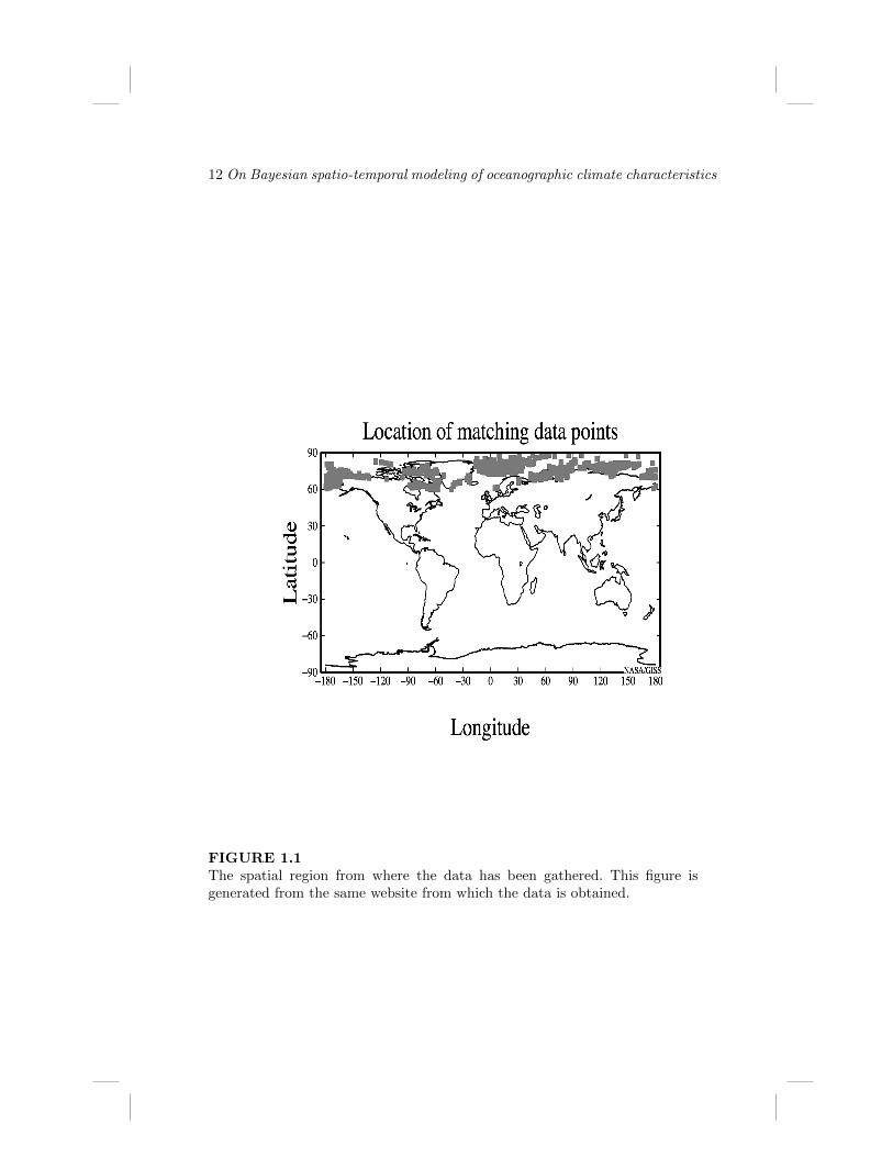
We access the data records from this source that correspond to Latitudevalues 60 degree North and higher. We further limit that data to be from 1975or more recent times. The region from which the data has been gathered isdepicted in Figure 1.1. This map has been produced by the afore-mentionedwebsite.

1.3 A description of the methodology

We consider the variables temperature, salinity, and the ratio of Oxygen-16 andOxygen-18 isotopes, called Oxygen-18 in the sequel. We might have consideredmodeling for the hydrogen and deuterium isotope ratio, but only 8 recordsout of a total of 11800 contained values for these, the rest were missing.Consequently deuterium isotope ratio was not considered as a variable inthis study. There were some missing values in each of the other variables aswell, but not as overwhelming.

We consider observations from 60 North and above latitudes, which largelycorrespond to the Arctic Ocean region. The data is gathered at various depths,at different longitudes, over different months of the year, from 1975 onwards.Since data collection is sparse and uneven outside the summer months, we


restrict our attention to data from July-September only. We consider spatialblocks of data, in order to model spatial smoothness and coherence. In theanalysis presented below, we consider four bands of latitude values (60-70,70-75, 75-80 and 80-90 North), ten levels for longitude values produced by thefollowing break points (-160, -80, -40, -5, 0, 20, 40, 90, 130, 180), and elevenlevels of depths (bins separated at depth values of 0, 5, 15, 30, 50, 100, 150,300, 500, 1000, 10000). These choices were made keeping data availability inmind. Note that the latitude, longitude and depth bands of values have a nat-ural ordering each. Thus, spatial dependence may be modeled by consideringneighboring bands. In view of the circular nature of longitudes, an additionalconstraint is imposed.

A generic notation for a data point may be Y (`1, `2, d, t, j), where `1 spec-ifies the latitude level, `2 the longitude level, d the depth level, t the time, andj an oceanic feature (temperature, salinity, O-18 ratio). We might further col-lapse the first four indices (latitude, longitude, depth and time), and considera generic observation yi ∈ R3 as a feature vector indexed by space-time.

For each observed sample point i = 1, . . . , n (n = 6795 number of samples)and N(= 3) number of response variables, we assume the following model:

[yi|ηi,Θi] ∼ N3 (ηi,Θi) ,

where ηi is the mean vector ∈ RN , and Θi is the corresponding precisionmatrix. Notice that these vary with the observed sample points.

We assume that the mean function ηi are affected by the spatial inter-dependence between the response variables, and not the variance-covariancestructures.

In the above the the precision matrices Θi are allowed to be differentfor different observations, with identical distributions for different levels oflongitude and depth. Suppose

τ1 ∼Wishart(IN , N),

is a N × N random matrix. Here IN is the identity matrix of dimension N .The degrees of freedom parameter is set at N as this corresponds to the leastinformative proper prior. For observations at a given level of longitude anddepth values, we use the prior that the precision matrices Θi are distribu-tionally identical copies of the corresponding τ1 matrices. Thus, geographiclocations were assumed to have exchangeable prior distributions which in thiscase expressed for the precision matrices as Wishart distributions with pre-fixed hyper-parameters.

We use a spatially smoothed dynamic linear model for the mean vectors.The response variables are assumed to have individual overall means withvariation around it depending upon geographical location given by the tripletlatitude, longitude and depth. Initial data exploration suggested that the be-havior of the response variables at various depths is possibly non-smooth. Thussmoothness on the remaining 2-dimensional surface were explored and the fol-


lowing model describes possibilities of using lags in both (latitude, longitude)and (longitude).

The additive model for the mean vectors are given by, for i = 1, . . . , n andj = 1, 2, 3(= N),

ηi,j = µ0j + µlati,longi,depthi,j .

Here the overall effect vector is modeled with multivariate normal distributionas follows:

µ0 ∼ NN (03×1, IN ) .

We have a more complex modeling structure for the space-dependent meanstructure, as follows:

µ (k, `,m) =

0, if ` = 1, for all k, m,∼ NN (µ (k, l − 1,m, 1 : N) , τN×N )

if k = 1, ` = 2, . . . , 10 and all m∼ N3 (0.5µ(k − 1, `,m) + 0.5µ(k, l − 1,m), τN×N )

for allm, k = 2, . . . , 4 and ` = 2, . . . , 10.

The hyper-parameter τ appearing above is given a Wishart distribution inthis hierarchical structure.

τ ∼Wishart (IN×N , N) .

In the above framework, the spatial dependence within a given block of(latitude, longitude, depth)-level is captured by common parameters, whilebetween block dependencies are captured by shared hyper-parameters. Tem-poral dependencies are captured by the built-in dependence structure for eachlongitude and depth block in the precision matrices Θi’s, and in the shareddependencies in the ηi’s. Note that it is guaranteed that we have a proper pos-terior distribution, since all the priors were chosen to be probability densitymeasures. This model can be enhanced with more complex features. However,our analysis showed that adding more complexity either by more complexmean and dispersion structures, or with additional spatial or temporal depen-dency measurements, does not enhance the quality of the statistical model.This is at least partially because of the nature of the data, and in keepingwith the results of earlier, non-Bayesian attempts at analyzing this data, see[5, 23]. In addition, this feature of additional complexity not leading to modelimprovement strongly suggest that this problem is M -open. A Bayesian anal-ysis problem is considered M -open if the data generating mechanism is notwithin the collection of models used for analysis, and there is no prior belief onhow the data related to the “true model”. One of the most important reasonfor analyzing climate data is for predicting future climate patterns, especiallyin a climate-change regime. It may be noted that prediction presents uniquechallenges in M -open problems, see [6, 7, 8] for detailed discussion on suchissues.


1.4 Results

We run a Markov Chain Monte Carlo procedure according to the model spec-ified above, to generate an approximate posterior distribution of the param-eters of interest. We used 2 parallel chains, and a burn-in of 10,000 for eachchain, followed by a further sequence of 50,000 iterations, which we thinnedby a factor of 10. This allowed us to generate posteriors summaries based on(2 x 50000 / 10 =) 10000 samples, which are presented below.

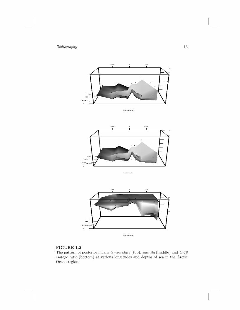
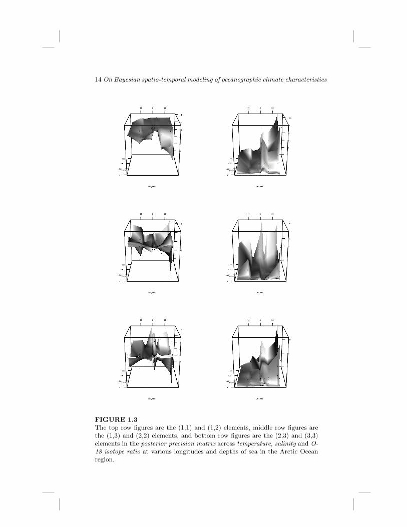
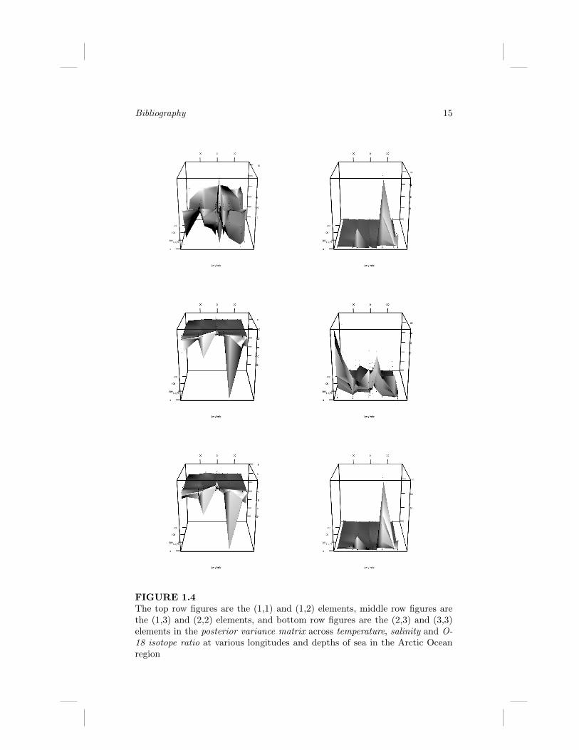
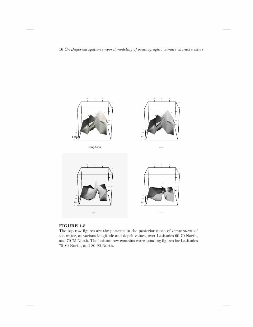
In Figure 1.2, we show how the three response variables, (temperature,salinity and O-18 isotope ratio) varies with depth and longitude. Figure 1.3show how the elements of the precision matrix, denoting the joint variabilityof the three responses, vary across depth and longitude. The figures for thecorresponding posterior variance matrix over these three responses is given inFigure 1.4. In Figure 1.5, Figure 1.6 and Figure 1.7, we present the posteriordistributions of these three responses as various latitude values.

Our major conclusion from this quite extensive analysis is that oceanvariables are co-dependent, their mean and covariance structures seem to bestrongly related to the spatial and temporal frames from which the observa-tions have been gathered. There are naturally some differences between thevariables, and some scope of bringing in Physics-guided knowledge amongthe response variables we studied. The patterns we found in the data suggestthat no simple relationship would possibly suffice to explain the nature ofany one of the response variables over space and time, or for the nature ofco-dependence among the variables themselves. The figures we have presentedshow that the lack of a simple relationship should not be confused with a lackof a relationship; there is very strong suggestion of a pattern, see Figure 1.2for example. One common theme that emerges from these graphics is thatthe posterior is nether simple, nor smooth over space, and standard summarymeasures like posterior location or scale parameters may be misleading.

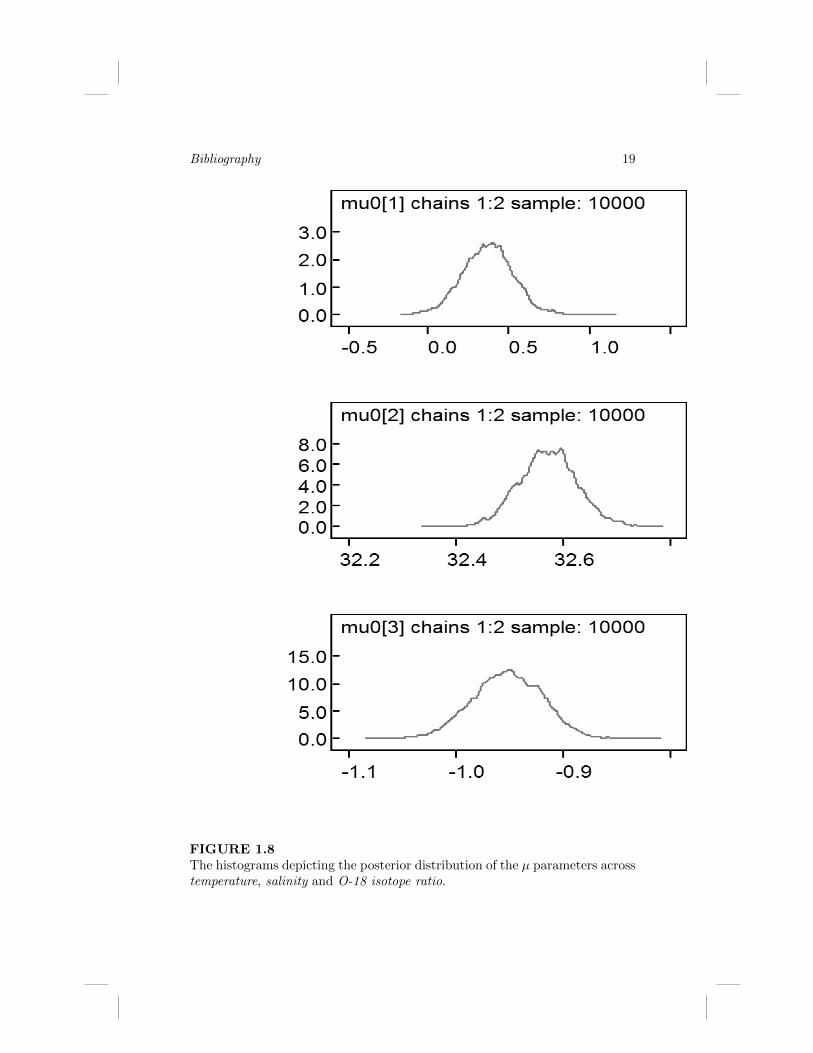
We now present some evidence about the performance of the MarkovChain Monte Carlo procedure we adopted. In Figure 1.8 we show the pos-terior histogram of the µ-parameters for the three responses. The precisionτ -parameters have posterior histograms as shown in Figure 1.9. Various di-agnostic results, for example convergence graphs, posterior deviance results,auto-correlation plots are presented in Figure 1.10.

These results strongly suggest that the extracted samples from the MCMCruns may resemble a sample from the true posterior distribution of the variousparameters under consideration. We have performed some robustness studies,whereby our conclusions do not seem to be altered by a choice of hyper-parameter values.


1.5 Discussion

The existing literature on climate modeling is essentially one of modeling na-ture using knowledge from a variety of scientific disciplines. From a Physics-based perspective, it is typical to consider the variable under study as a de-terministic, but extremely complex, function of other physical variables. Thiskind of modeling retains a high degree of fidelity to the true process by whichthe data is generated. However, it is inevitable that not all features of a systemas complex as climate will be measured or retained in various forms of datarecords. Also, our present state of knowledge about how different physical,atmospheric, geophysical and other variables interplay is limited, as is naturalin any scientific discipline. A very partial and incomplete review of naturalscientific modeling of climate may be obtained from [14], [22], [9], [11] andseveral references therein. A Bayesian framework where such Physics-basedapproach may be considered may be obtained from [17].

Climate models are used for several purposes. Of these, some of the moreimportant ones are detection of climate change, attribution of climate changeto a cause, forecasting of future climate scenarios. A study of climate in thepre-historic past, using data and proxies based on tree-rings, ice-core samplesand other geophysical and fossilized sources, forms the topic of paleoclimate,and is useful as a reference for climate as of today and in future. Examples ofpaleoclimate studies may be found in [20], [19] [1], [15], [13] and other sources.

Climate research has progressed beyond change detection and attribution.Forecasts, and quantifying errors of forecasts relating to future climate sce-narios, predicting possible consequences of climate change; combination ofoutputs from several AOGCM models, and other important studies now forma part of climate research. Several works using Bayesian ideas have contributedto this research, see, for example [3], [18], [2], [27] and references therein. Inmuch of the above cited literature, oceanographic variables have not been con-sidered. This is partially because the atmosphere is better understood than thehydrosphere in Physics, partially because it was felt that modeling the atmo-sphere was of greater importance for understanding climate change. However,in recent times, the hydrosphere, cyrosphere, biosphere are being studied withgreater vigor.

In this context, this paper attempts to present a Bayesian analysis of athree-dimensional response on ocean water. We illustrated the complexity ofpatterns in oceanographic variables, and suggested a possible approach to-wards understanding the statistical properties of these variables. While a moredetailed and thorough study needs to be done, our MCMC results suggest thata Bayesian approach may provide answers to several interesting questions inthis domain.

In addition, the possibility of analyzing data from M -complete and M -open problems using the broad framework we adopted here: namely, con-


structing blocks of indexing variables to reduce or eliminate data sparsity,using least informative proper priors, and assuming minimal structure other-wise, should be explored.

Acknowledgment: We thank two anonymous referees for their com-ments, which greatly improved this paper. The second author’s research waspartially funded by NSF grants # SES-0851705 and # IIS-1029711, and re-search grants from the Institute on the Environment and College of LiberalArts, University of Minnesota.

Bibliography

[1] Allen, M. R. and Tett, S. F. B. (1999) Checking for model consis-tency in optimal fingerprinting. Clim. Dyn. 15, 419–434

[2] Berliner, L. M., Levine, R. A. and Shea, D. J. (1999) BayesianClimate Change Assessment, J. Climate, 13, 3805-3820.

[3] Berliner, L. M., Nychka, D. and Hoar, T. (2000) Studies in the At-mospheric Sciences (2000) edited by Mark L. Berliner, Douglas Nychka,Timothy Hoar; Springer, New York.

[4] Bernardo, J. and Smith, A. (2000) Bayesian Theory, John Wiley,Chichester.

[5] Chatterjee, S., Deng, Q., and Xu, J. (2009) The statistical evidenceof climate change: an analysis of global seawater data technical report#677, School of Statistics, University of Minnesota.

[6] Clarke, B. (2010) Desiderata for a predictive theory of statisticsBayesian Analysis, 5, (2), 283-318.

[7] Clarke, J. L., Clarke, B. and Yu, C.-W. (2013) Prediction in M -complete problems with limited sample size. Bayesian Analysis, 8, (3),647-690.

[8] Clyde, M. and Iversen, E. S. (2013) Bayesian model averaging in theM-open framework. In Bayesian Theory and Applications, ed. P. Damien,P. Dellaportas, N. G. Polson, and D. A. Stephens, pages 483-498, OxfordUniversity Press.

[9] Cox, P. M., Betts, R. A., Bunton, C. B., Essery, R. L. H., Rown-tree, P. and Smith, J. (1999) The impact of new land surface physicson the GCM simulation of climate and climate sensitivity. Clim. Dynam.15, 183–203.

[10] Durack, P. J., Wijffels, S. E., and Matear, R. J. (2012). Oceansalinities reveal strong global water cycle intensification during 1950 to2000. Science, 336(6080), 455-458.

[11] Giorgi, F. and Mearns, L. O. (2002) Calculation of Average, Uncer-tainty Range, and Reliability of Regional Climate Changes from AOGCM

9


Simulations via the ”Reliability Ensemble Averaging” (REA) Method, J.Climate, 10, 1141-1158.

[12] Gouretski, V., and Reseghetti, F. (2010). On depth and tempera-ture biases in bathythermograph data: Development of a new correctionscheme based on analysis of a global ocean database. Deep Sea ResearchPart I: Oceanographic Research Papers, 57(6), 812-833.

[13] Hegerl, G. C. and others (2006) Climate change detection and at-tribution: beyond mean temperature signals, J. Climate, 19, 5058-5077.

[14] IPCC (2008) Climate Change 2007, Cambridge University Press, U.K.

[15] The International ad hoc detection and attribution group(2005) Detecting and attributing external influences on the climate sys-tem: a review of recent advances J. Climate, 18, 1291-1314.

[16] Key, R.M., Kozyr, A., Sabine, C.L., Lee, K., Wanninkhof, R.,Bullister, J., Feely, R.A., Millero, F., Mordy, C. and Peng,T.-H. (2004). A global ocean carbon climatology: Results from GLODAP.Global Biogeochemical Cycles 18, GB4031.

[17] Kennedy, M. and O’Hagan, A. (2001). Bayesian calibration of com-puter models (with discussion). J. Royal Statist. Soc., Series B. 63, 425-464.

[18] Levine, R. A. and Berliner, L. M. (1999) Statistical Principles forClimate Change Studies, J. Climate, 12, 564-574.

[19] Li, B., Nychka, W. D. and Ammann, C. M. (2007) The ”HockeyStick” and the 1990s: A statistical perspective on reconstructing hemi-spheric temperatures Tellus, 59, 591-598.

[20] Mann, M. E., Bradley, R. S. and Hughes, M. K. (1998) Global-scale temperature patterns and climate forcing over the past six centuries.Nature 392, 779–787.

[21] Matsumoto, K.; Gruber, N. (2005). How accurate is the estimationof anthropogenic carbon in the ocean? An evaluation of the DC* method.Global Biogeochem. Cycles 19. doi:10.1029/2004GB002397.

[22] Mearns, L. O., Hulme, M., Carter, T. R., Leemans, R., Lal,M. and Whetton, P. (2001) Climate scenario development. In Climatechange 2001: the scientific basis (eds J. T. Houghton et al.). Contributionof working group I to the third assessment report of the Intergovernmen-tal Panel on Climate Change, pp. 739–768. Cambridge, UK: CambridgeUniversity Press.

Bibliography 11

[23] Mukherjee, U. and Chatterjee, S. (2013) A Fay-Herriot type ap-proach for better prediction in multi-indexed response with applicationto Arctic seawater data analysis, preprint.

[24] Orr, J. C. et al. (2005). Anthropogenic ocean acidification over thetwenty-first century and its impact on calcifying organisms. Nature 437,681-686.

[25] Raven, J. A. et al. (2005). Ocean acidification due to increasing at-mospheric carbon dioxide. Royal Society, London, UK

[26] Schmidt, G.A., G. R. Bigg and E. J. Rohling (1999) ”Global Sea-water Oxygen-18 Database,” http://data.giss.nasa.gov/o18data/

[27] Tebaldi, C., Smith, R. W., Nychka, D. and Mearns, L. O. (2005)Quantifying uncertainty in projections of regional climate change: aBayesian approach to the analysis of multi-model ensembles. J. Clim.18, 1524–1540.


FIGURE 1.1The spatial region from where the data has been gathered. This figure isgenerated from the same website from which the data is obtained.

Bibliography 13

FIGURE 1.2The pattern of posterior means temperature (top), salinity (middle) and O-18isotope ratio (bottom) at various longitudes and depths of sea in the ArcticOcean region.


FIGURE 1.3The top row figures are the (1,1) and (1,2) elements, middle row figures arethe (1,3) and (2,2) elements, and bottom row figures are the (2,3) and (3,3)elements in the posterior precision matrix across temperature, salinity and O-18 isotope ratio at various longitudes and depths of sea in the Arctic Oceanregion.

Bibliography 15

FIGURE 1.4The top row figures are the (1,1) and (1,2) elements, middle row figures arethe (1,3) and (2,2) elements, and bottom row figures are the (2,3) and (3,3)elements in the posterior variance matrix across temperature, salinity and O-18 isotope ratio at various longitudes and depths of sea in the Arctic Oceanregion


FIGURE 1.5The top row figures are the patterns in the posterior mean of temperature ofsea water, at various longitude and depth values, over Latitudes 60-70 North,and 70-75 North. The bottom row contains corresponding figures for Latitudes75-80 North, and 80-90 North.

Bibliography 17

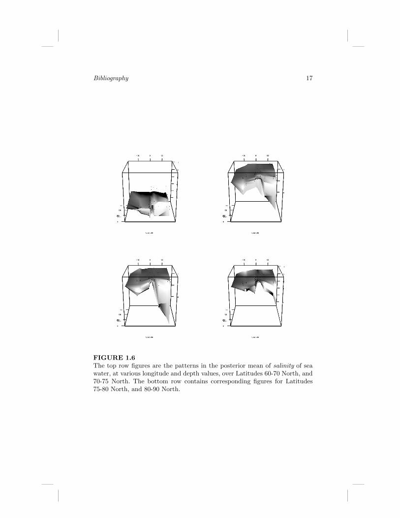
FIGURE 1.6The top row figures are the patterns in the posterior mean of salinity of seawater, at various longitude and depth values, over Latitudes 60-70 North, and70-75 North. The bottom row contains corresponding figures for Latitudes75-80 North, and 80-90 North.


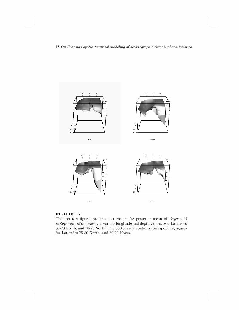
FIGURE 1.7The top row figures are the patterns in the posterior mean of Oxygen-18isotope ratio of sea water, at various longitude and depth values, over Latitudes60-70 North, and 70-75 North. The bottom row contains corresponding figuresfor Latitudes 75-80 North, and 80-90 North.

Bibliography 19

FIGURE 1.8The histograms depicting the posterior distribution of the µ parameters acrosstemperature, salinity and O-18 isotope ratio.


FIGURE 1.9The top row figures are the histograms of the (1,1) and (1,2) elements, middlerow figures are the histograms of the (1,3) and (2,2) elements, and bottomrow figures are the histograms of the (2,3) and (3,3) elements depicting theposterior distribution of the precision matrix across temperature, salinity andO-18 isotope ratio.

Bibliography 21

FIGURE 1.10Graphs denoting convergence properties, deviance, and autocorrelation struc-tures in the MCMC runs.

Documents

On Bayesian spatio-temporal modeling of …users.stat.umn.edu/~chatt019/Research/Papers/SCChapter.pdfrelating to adaptation and mitigation strategies to counter climate change,