Recent Linear Programming Developments for Operations Research and Management

Science

Yinyu Ye

Management Science and EngineeringStanford University

(Nanjing University, Beijing University)

INFORMS I 2012

1975 National Medal of Science

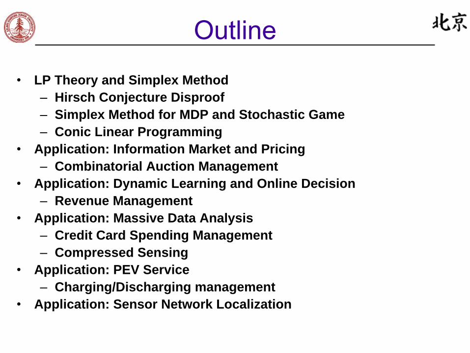
Outline

•

LP Theory and Simplex Method–

Hirsch Conjecture Disproof–

Simplex Method for MDP and Stochastic Game–

Conic Linear Programming•

Application: Information Market and Pricing–

Combinatorial Auction Management•

Application: Dynamic Learning and Online Decision–

Revenue Management•

Application: Massive Data Analysis–

Credit Card Spending Management–

Compressed Sensing•

Application: PEV Service–

Charging/Discharging management•

Application: Sensor Network Localization

Disprove Hirsch Conjecture

•

Warren Hirsch conjectured in 1957 that the diameter of the graph

of a polyhedron defined by n inequalities in d dimensions is at most n-d, and this conjecture was open till 2010.

•

There is a 43-dimensional polytope

with 86 facets and of diameter at least 44.

•

There is an infinite family of non-Hirsch polytopes

with diameter (1 + ε)n, even in fixed dimension.

(Francisco Santos 2010)

Markov Decision Process

•

Markov decision processes (MDPs) provide a mathematical framework for modeling sequential decision-making in situations where outcomes are partly random and partly under the control of a decision maker.

•

MDPs

are useful for studying a wide range of optimization problems solved via dynamic programming, where it was known at least as early as the 1950s (cf. Shapley 1953, Bellman 1957).

•

Modern applications include dynamic planning, reinforcement learning, social networking, and almost all other dynamic/sequential decision making problems in Mathematical, Physical, Management and Social Sciences.

A Simple MDP Problem I

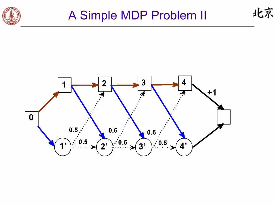
A Simple MDP Problem II

Cost-to-Go in MDP

Taken actions in Red

Greedy Simplex Rule

Taken actions in Red

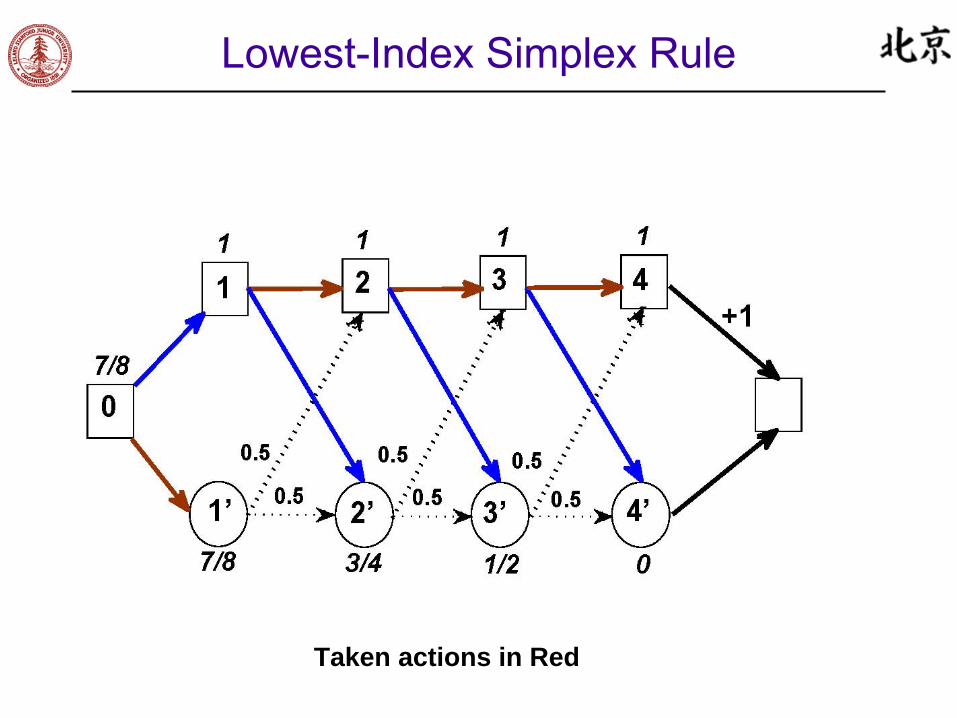
Lowest-Index Simplex Rule

Taken actions in Red

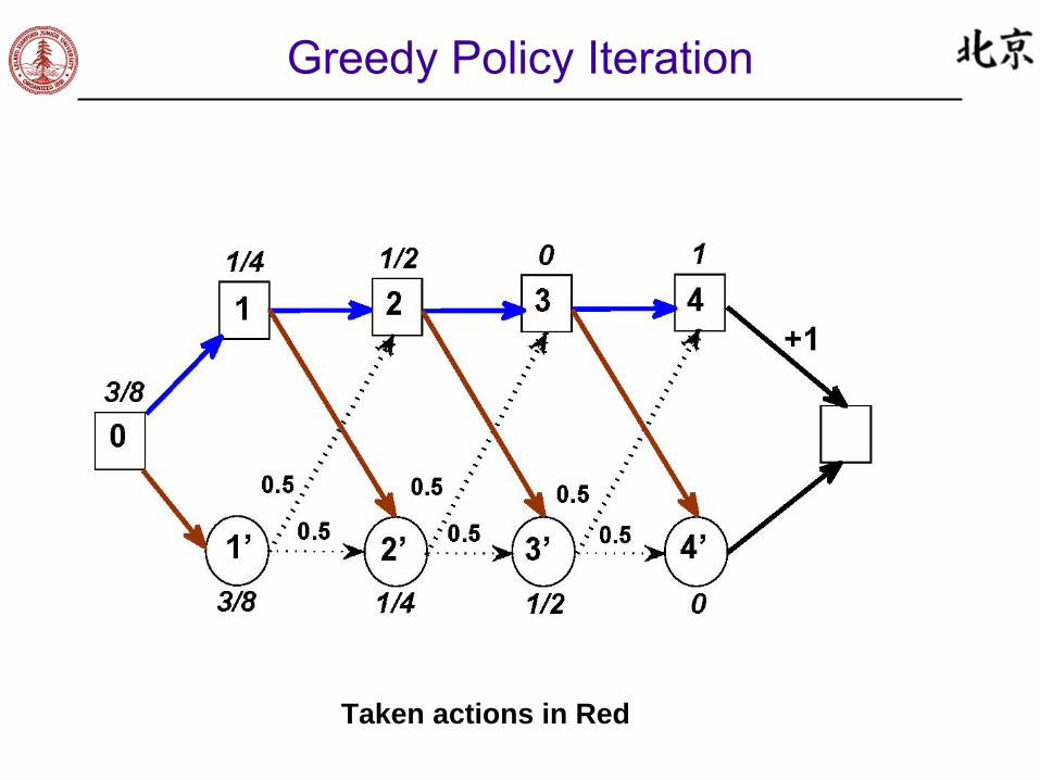
Greedy Policy Iteration

Taken actions in Red

Complexity of Simplex/Policy Methods

•

The classic simplex and policy iteration methods, with the greedy pivoting rule, are strongly polynomial-time algorithms for MDP with fixed discount rate. (Y, 2011)

•

The complexity of the policy iteration method is an m factor less than that of the simplex method. (Hansen, Miltersen, and Zwick, 2011).

•

The policy iteration method, with the greedy pivoting rule, is a strongly polynomial-time algorithms for Turn-

Based Two-Person Zero-Sum Stochastic Game with fixed discount rate. (Hansen, Miltersen, and Zwick, 2011).

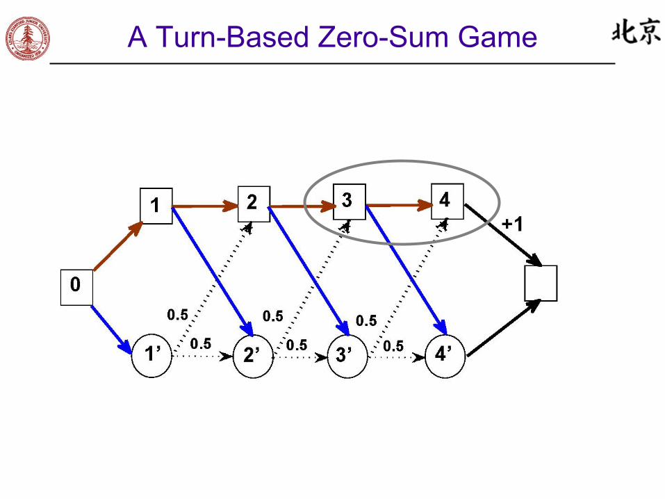
A Turn-Based Zero-Sum Game

Conic Linear Programming

*i

ii

iii

ii

KS

C,SAyts

yb

K X,...,m,,ibXAts

X C

..

Maxmize

1 ..

Minimize

Conic Linear Programming I

•

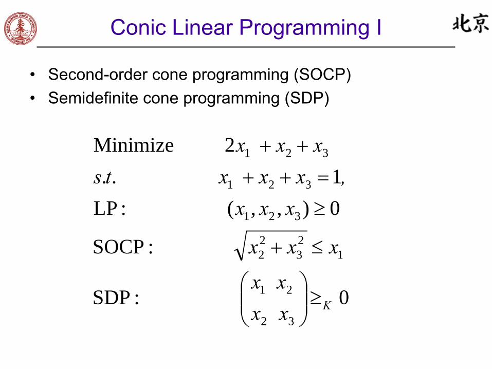
Second-order cone programming (SOCP)•

Semidefinite cone programming (SDP)

0

:SDP

:SOCP

0),,( :LP1 ..

2 Minimize

32

21

123

22

321

321

321

Kxxxx

xxx

xxx,xx xts

xx x

Conic Linear Programming II

There are efficient polynomial-time algorithms for conic linear programming

(Nesterov and Nemirovskii

1992, Alizadeh

1992, etc.)

For certain NP-hard problems, conic linear programming Provide tighter relaxation than that of LP

(Goemans

and Williamson 1995, etc.)

World Cup Betting Example

•

Market for World Cup Winner–

Assume 5 teams have a chance to win the 2006 World Cup: Argentina, Brazil, Italy, Germany and France

–

We’d like to have a standard payout of $1 if a participant has a claim where his selected team won

•

Sample Orders

Order Number

Price Limit

Quantity Limit q

Argentina Brazil Italy Germany France

1 0.75 10 1 1 1

2 0.35 5 13 0.40 10 1 1 14 0.95 10 1 1 1 15 0.75 5 1 1

Markets for Contingent Claims

•

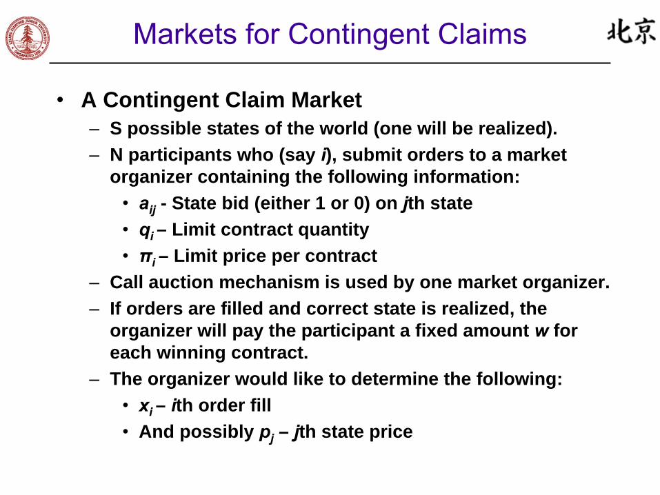
A Contingent Claim Market–

S possible states of the world (one will be realized).–

N participants who (say i), submit orders to a market organizer containing the following information:

•

aij

- State bid (either 1 or 0) on jth state•

qi

– Limit contract quantity•

πi

– Limit price per contract–

Call auction mechanism is used by one market organizer.–

If orders are filled and correct state is realized, the organizer will pay the participant a fixed amount w for each winning contract.

–

The organizer would like to determine the following:•

xi

– ith order fill•

And possibly pj

– jth state price

Central Organization of the Market

•

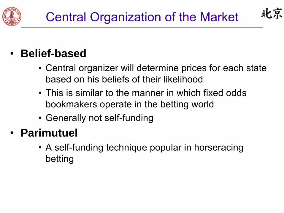
Belief-based•

Central organizer will determine prices for each state based on his beliefs of their likelihood

•

This is similar to the manner in which fixed odds bookmakers operate in the betting world

•

Generally not self-funding•

Parimutuel

•

A self-funding technique popular in horseracing betting

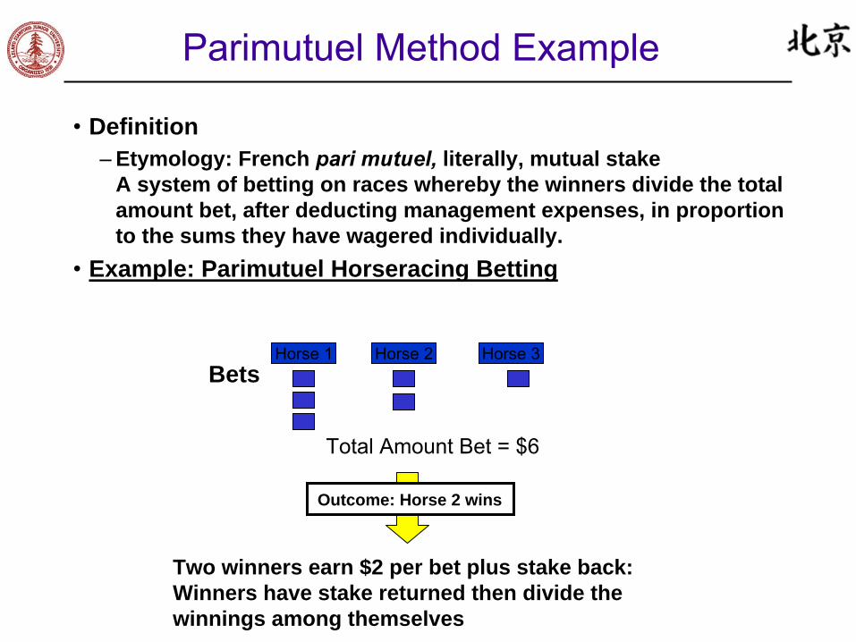
Parimutuel Method Example

•

Definition–

Etymology: French pari

mutuel, literally, mutual stake A system of betting on races whereby the winners divide the total amount bet, after deducting management expenses, in proportion to the sums they have wagered individually.

•

Example: Parimutuel Horseracing Betting

Horse 1 Horse 2 Horse 3

Two winners earn $2 per bet plus stake back: Winners have stake returned then divide the winnings among themselves

Bets

Total Amount Bet = $6

Outcome: Horse 2 wins

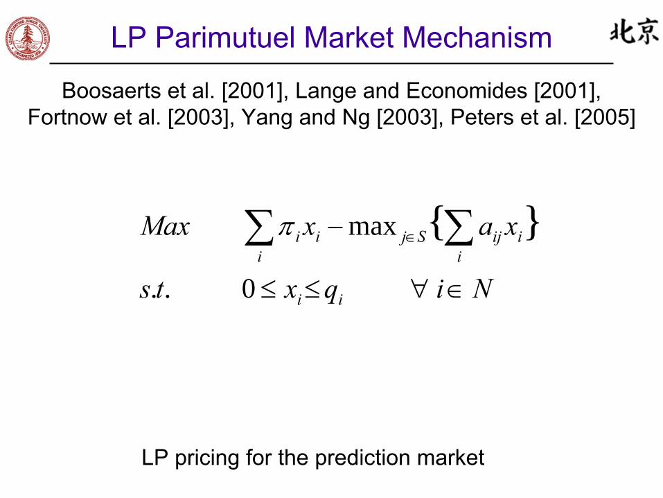
LP Parimutuel

Market Mechanism

Boosaerts

et al. [2001], Lange and Economides [2001], Fortnow

et al. [2003], Yang and Ng [2003], Peters et al. [2005]

Niqxts

xaxMax

ii

iiij

iSjii

0..

max }{

LP pricing for the prediction market

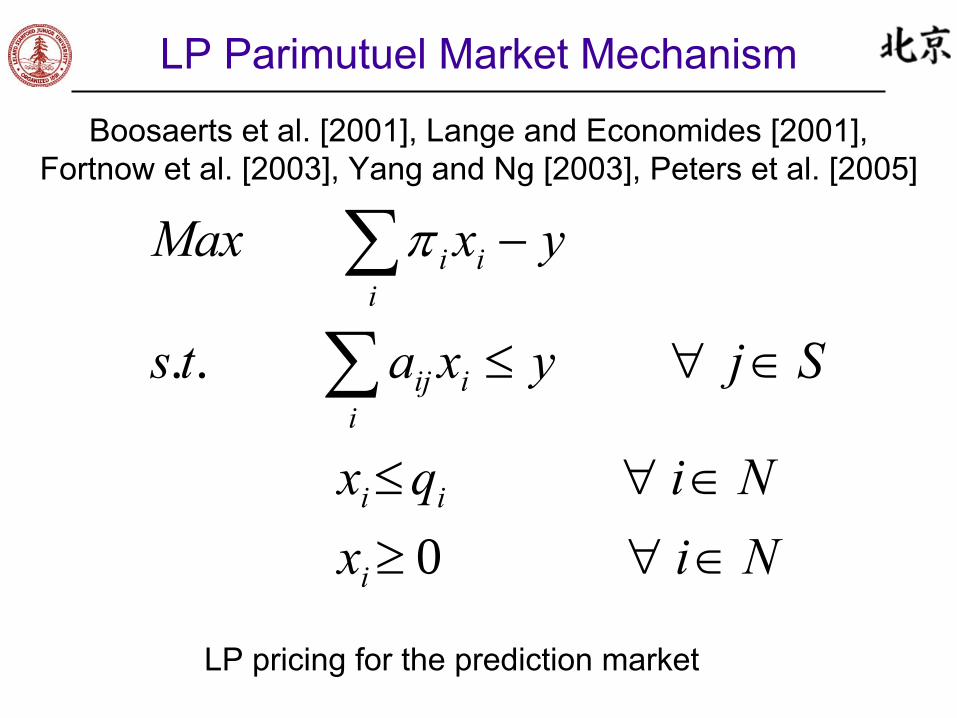
LP Parimutuel

Market Mechanism

Boosaerts

et al. [2001], Lange and Economides [2001], Fortnow

et al. [2003], Yang and Ng [2003], Peters et al. [2005]

NixNiqx

Sjyxats

yxMax

i

ii

iiij

iii

0

..

LP pricing for the prediction market

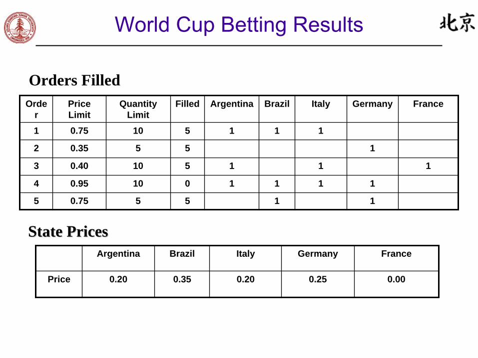
World Cup Betting Results

Orders FilledOrde

rPrice Limit

Quantity Limit

Filled Argentina Brazil Italy Germany France

1 0.75 10 5 1 1 1

2 0.35 5 5 1

3 0.40 10 5 1 1 1

4 0.95 10 0 1 1 1 1

5 0.75 5 5 1 1

Argentina Brazil Italy Germany France

Price 0.20 0.35 0.20 0.25 0.00

State PricesState Prices

The MS&E 211 Auction Game

•

Each student is given $500•

Students submit bids to earn bonus points for each game

•

They learn how the market maker makes decisions and how the mechanism works

•

Students create new mechanisms

•

Two students have applied the LP mechanism to real biddings

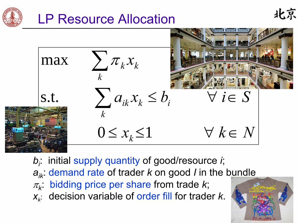
LP Resource Allocation

Nkx

Sibxa

x

k

kikik

kkk

10

s.t.

max

bi

: initial supply quantity

of good/resource i;aik

: demand rate

of trader k

on good I

in the bundlek

: bidding price per share

from trade k;xk

: decision variable of order fill

for trader k.

On-Line Resource Allocation LP

•

Traders come one by one

sequentially, buy or sell, or combination, with a combinatorial order/bid (ak

,k

)•

The seller/market-maker has to make an order-fill decision as soon as an order arrives

•

The seller/market-maker faces a dilemma:–

To sell or not to sell, and by how many

•

Policy or Mechanism Design

Desirable Properties of Mechanism

•

Efficient computation for making a decision sequentially–

Forward dynamic decision making and price update for each good

•

Near off-line optimality–

The (expected) revenue of the on-line models would be close to that of the off-line model

•

Risk attitude of the market maker–

Market maker takes a certain risk attitude when filling orders•

Truthfulness (in myopic sense) –

Bidding true value of a bet should be dominant strategy for each trader (if he or she is a one-time trader)

LP Dynamic Learning Mechanism

Assume that the orders arrive randomly:•

There exist an asymptotically optimal dynamic learning mechanism for the on-line LP recourse model.

(Agrawal, Wang, and Y 2010).•

The mechanism is based on dynamically updating the dual prices of the LP model from revealed data.

•

Dynamic learning is superior to one-time learning(1 -

ε1/2) vs

(1-ε1/3)

•

The pace of learning is carefully managed, neither too slow nor too fact.

•

The analysis is based on expected revenue.

Convex Programming Mechanism on Risk

•

As soon as bid (a,) arrives, market maker solves

where

the ith

entry of

q is the quantity already sold

to

earlier traders, x

is the order fill variable for the new order, and

u(s)

is any concave and increasing

value function of remaining good quantity vector,

s.

(Agrawal et al. 2011, OR)

1 , s.t.

)( max }{

x0x

uπxx,

qbsa

ssAvailable good quantity for allocation

Immediate revenue Future value

Rational of the Model/Mechanism

•

Maximization principle: to maximize the sum of the immediate revenue, x, and a value/utility function, u(s), on the remaining good inventory.

•

Initial prices on goods: represented by the derivatives of u, that is,

p=∇u (

b ).

•

Price update: the optimal Lagrange multipliers

of this convex optimization problem

with maximizers (x*,s*), that is,

*)(* sp u

u(.)

Determines Mechanism Properties

Choose

u(s)

such that•

to approximate future revenue and reserve prices

•

to bound the worst case regret/revenue loss•

to learn good prices

with risk measures

•

to guarantee propernessCharge the trader such that•

traders would bid truthfully

Theorem: A dynamic pricing rule is proper if and only ifu(s)

is a proper concave function

Business or Personal?

Is the transaction for business or personal when a business- credit card is being used?

Data Analytics

$210

$195

$200

Actual

…

$60

$0

$25

n

$35$134$0…

$0$25$2002

$87$0$1561

…321Account

Each Column representsan Industry Code Personal Remittances

Value of transactions in

period

For each of the industry codes, the model will determine a probability which indicates the likelihood that a transaction was personal.

Model Example

For each of the industry codes, the model will determine a probability (in red) which indicates the likelihood that a transaction was personal. The goal is to minimize the sum of the squares of the differences (in blue).

$210

$195

$200

Actual

5%…0%10%25%

$60

$0

$25

n

$230

$200

$244

Predicted

$20$35$134$0…

$5$0$25$2002

$44$87$0$1561

Difference…321Account

Each Column representsan Industry Code Personal Remittances

Probability Personal

Value of transactions in

period

Regression Model

•

Let xj

be such a probability that a transaction is personal for industry code j•

ai,j

–

transaction amount for account i and industry code j•

bi –

amount paid by personal remit for account i•

∑j

ai,j

xj

–

the expected personal expenses for account i•

We’d like to choose xj

such that ∑j

ai,j

xj

matches bi

for ALL i

.,10s.t.

Min 2)(jx

bxa

j

jijij

i

Our model will determine the probability that a transaction from

each industry code is personal in such a manner which will minimize the sum of the squared errors (between predicted personal remittances and actual personal remittances).

Compressed Sensing

.,10s.t.

||||Min 1||jx

xbxa

j

jijij

i

To reduce the number of small probabilities or improve the sparsity

in the final solution

This is a linear program•Widely used in signal analyses and imaging construction•A recent theoretical analysis of compressed sensing using L1 regularization•Become a popular research topic

A Dynamic LP Algorithm for Facilitated Charging and

Discharging of Plug-In Electric Vehicles (Taheri, Entriken

and Y 2011)

Plug-In Electric Vehicle Network

•

Some estimates say there could be 100 million Plug-in Electric Vehicles (PEVs) on the road in the United States by 20301

•

The charging of PEVs

will add to the current load on the electricity grid. –

This addition to the load can be planned for and managed.

1EPRI PRISM Analysis, 2009

Motivation•

Construct a robust algorithm to dynamically assign low cost, feasible and satisfactory charging/discharging schedules for individual vehicles in a fleet

•

Lower the typical consumer cost of charging/discharging a PEV

•

Potential benefits to electric utilities of using PEVs

to provide grid services

Plug-In Electric Vehicle Network

Specific Problem Statement

The goal is to manage the charging of a fleet of PEVs so that:1. Every vehicle has enough energy in its battery to drive2. The cost of charging is low3. The peak electricity load does not increase or reduce4. Robust to deal with uncertainty

We construct an algorithm that establishes total fleet demand and makes instant decisions for individual vehicles based on:

•

Energy demand of each vehicle•

Electricity load capacity and scheduling obligation•

Current electricity and gasoline prices•

Individual Vehicle Characteristics

Aggregator

Real Data

Vehicle Driving Behaviors–

Obtained from the 2009 National Household Transportation Survey (NHTS) –

Helpful discussions and filtered data from Morgan and Christine–

The following results are based on data from urban California on

a MondayElectricity Load

–

Obtained from CAISO OASIS (Open Access Same-Time Information System)

–

Used the demand in the PG&E transmission access charge area for the week of August 22-28, 2011

Electricity and Gasoline Prices–

Electricity prices: PG&E baseline summer time of use rates –

Gasoline prices: mean gas price in the zip code 94305 on August 31

Clustering Method

•

Use the kmeans

clustering algorithm:–

On the normalized differential–

With the Euclidean distance

•

This algorithm attempts to put the vectors into clusters to minimize the average distance from the mean

Concept:

Cars driving in the same hours, for the same relative

amount should be in the same cluster

Concept:

Cars driving in the same hours, for the same relative

amount should be in the same cluster

Formulation Considerations•

There is an upper limit on the total amount of energy the fleet of vehicles uses to charge or discharge. –

This upper limit, or “charge cap”, is related to the current amount of electricity being used.

–

It can be also set as a variable to lower the peak demand

•

Decisions on charging/discharging schedules are made instantly

as vehicles plug in to the grid.

•

Vehicles can only fill the gas tank and generate electricity from the battery while driving, and can only charge or discharge the battery while not driving.

•

Solution: an LP optimization model

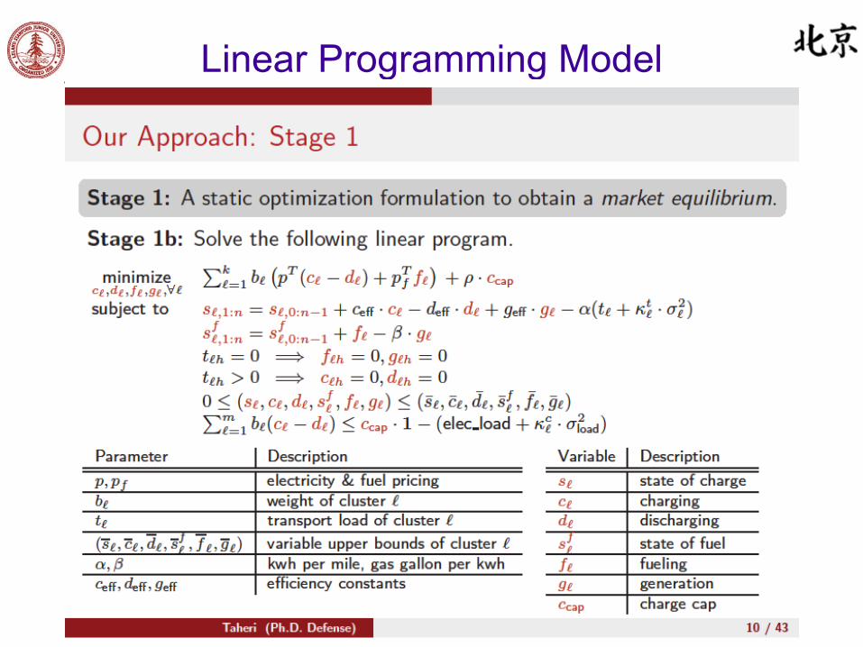
Linear Programming Model

Distributed Price Mechanism

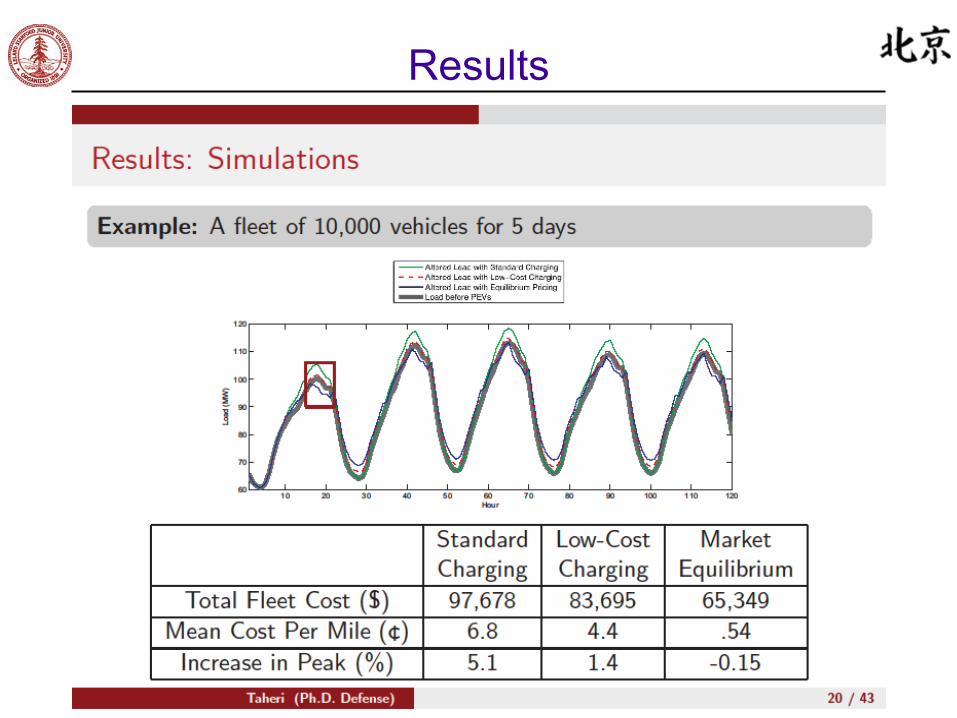
Results

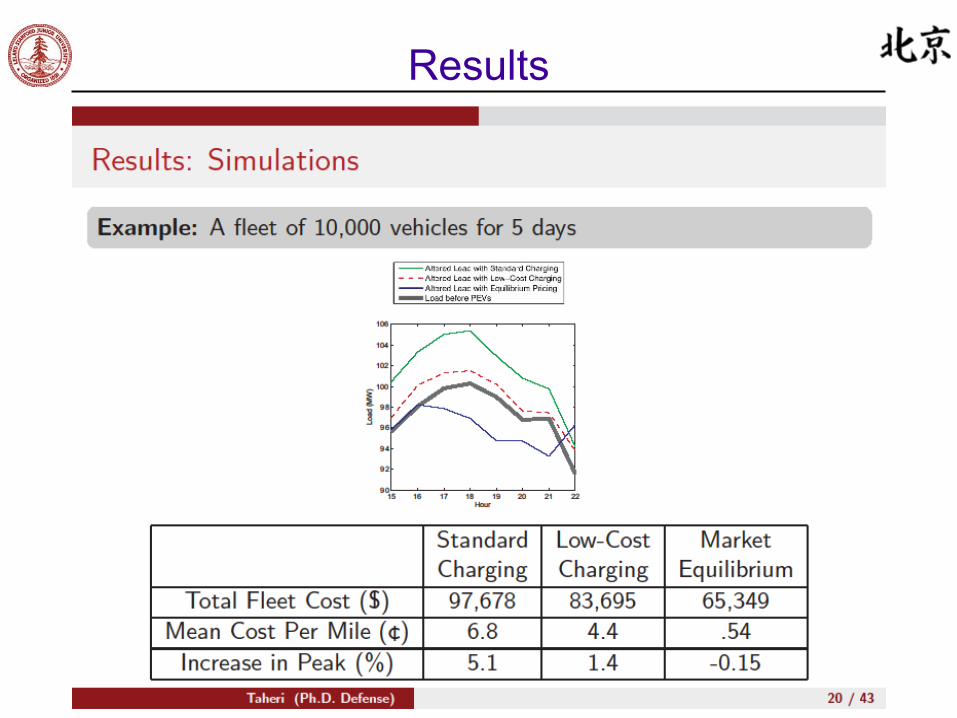
Results

Results

More Work on PEV

•

Fixed charging and discharging costs

•

Include features that take battery life into account

•

Make the charging schedules More robust to unexpected events

•

Game theoretical model among different agents

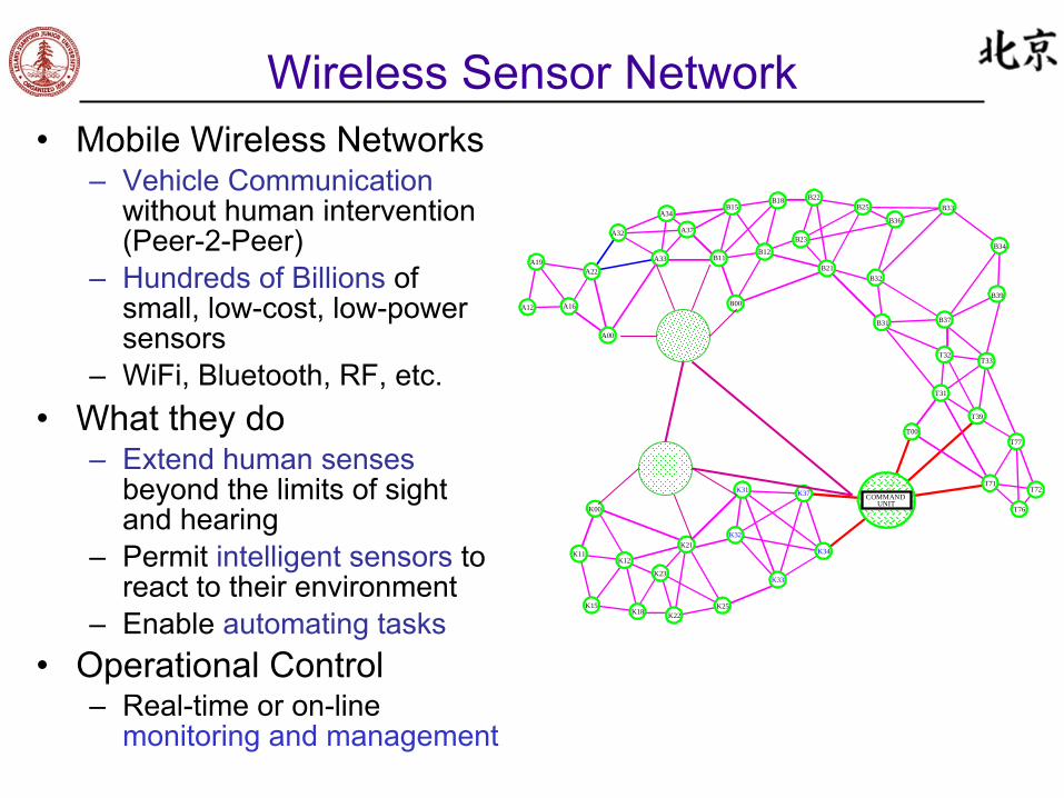
Wireless Sensor Network•

Mobile Wireless Networks–

Vehicle Communication

without human intervention (Peer-2-Peer)

–

Hundreds of Billions

of small, low-cost, low-power sensors

–

WiFi, Bluetooth, RF, etc.•

What they do–

Extend human senses

beyond the limits of sight and hearing

–

Permit intelligent sensors

to react to their environment

–

Enable automating tasks•

Operational Control–

Real-time or on-line monitoring and management

B11

B00A12

A00

A19

A16

T00

T32

T31

T39

T33

T77

T71T72

T76

K11K12

K00

COMMANDUNIT

B36

B39

A37

A34

A32

A33

A22

B15B18 B22

B23

B21

B25

B31

B32

B33

B34

B37

K15K18

K21

K23

K22K25

K31

K32

K33

K34

K37

B12

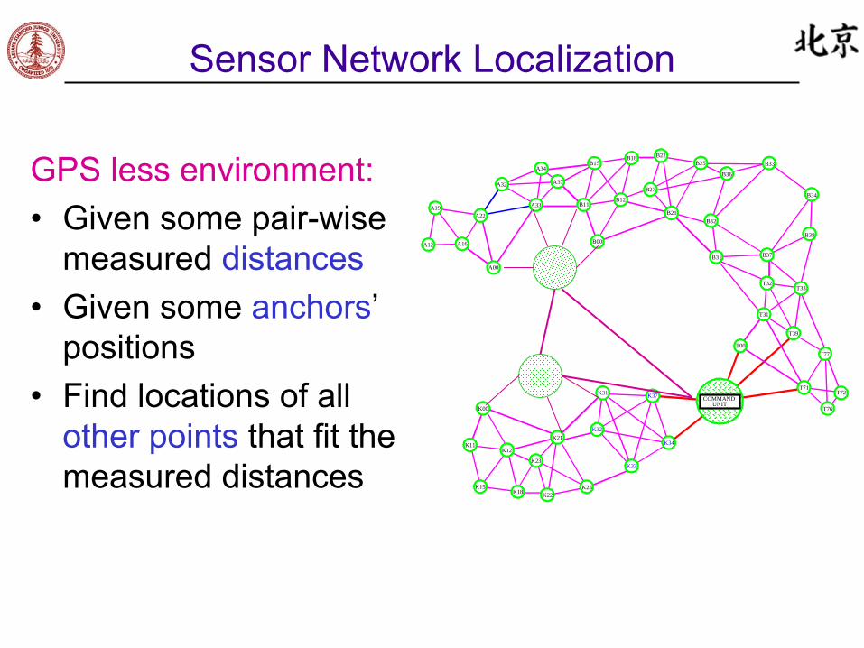
Sensor Network Localization

GPS less environment:•

Given some pair-wise measured distances

•

Given some anchors’ positions

•

Find locations of all other points

that fit the

measured distances

B11

B00A12

A00

A19

A16

T00

T32

T31

T39

T33

T77

T71T72

T76

K11K12

K00

COMMANDUNIT

B36

B39

A37

A34

A32

A33

A22

B15B18 B22

B23

B21

B25

B31

B32

B33

B34

B37

K15K18

K21

K23

K22K25

K31

K32

K33

K34

K37

B12

Firefighter Rescue Operation

•

When Firefighters are trapped or lost, there is no effective way to rescue them

•

Trapped or lost firefighters, if conscious, often don’t know their own location

•

Unlike the Movies, structural fires are characterized by heavy smoke and darkness

•

Sounds are diffused by smoke and difficult to localize

•

GPS is not available, and seconds count...

Vehicle-2-Vehicle Network Location

•

Vehicle-to-Vehicle Self-forming Mesh Network–

No fixed infrastructure for IR–

Communications using WiFi

•

Sensor Integration–

Traffic information–

Condition information

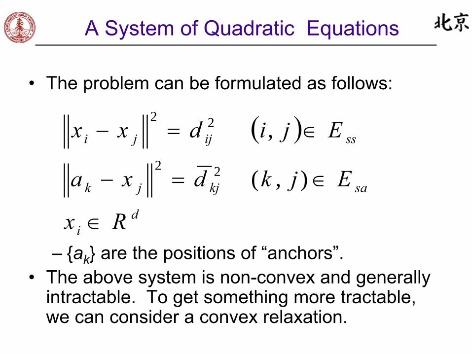
A System of Quadratic Equations

•

The problem can be formulated as follows:

–

{ak

} are the positions of “anchors”.•

Does it have a solution?

•

Is the solution unique?

di

sakjjk

ssijji

Rx

Ejkdxa

Ejidxx

),(

,

22

22

A System of Quadratic Equations

•

The problem can be formulated as follows:

–

{ak

} are the positions of “anchors”.•

The above system is non-convex and generally intractable. To get something more tractable, we can consider a convex relaxation.

di

sakjjk

ssijji

Rx

Ejkdxa

Ejidxx

),(

,

22

22

SDP Relaxation

•

Step 1: Linearization

jTjj

Tii

Tiji xxxxxxxx 2

2

jTjj

Tkk

Tkjk xxxaaaxa 2

2

SDP Relaxation

•

Step 1: Linearization

jTjj

Tii

Tiji xxxxxxxx 2

2

jTjj

Tkk

Tkjk xxxaaaxa 2

2

Yii Yij Yjj

Yjj

Biswas and Y 2004, So and Y 2005

SDP Relaxation

•

Step 1: Linearization

•

Step 2: Tighten

jTjj

Tii

Tiji xxxxxxxx 2

2

Yii Yij Yjj

jTjj

Tkk

Tkjk xxxaaaxa 2

2

Yjj

PSDYXXI

ZXXY TT

Biswas and Y 2004, So and Y 2005

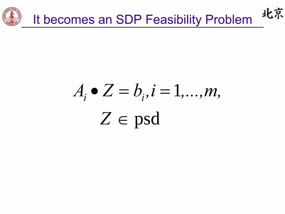
It becomes an SDP Feasibility Problem

psd 1

Z,...,m,,ibZA ii

Linear Programming Legacy Continues …

•Is there a strongly polynomial time algorithm for LP?

•Solve LPs with a huge size (billion-dimension)

•Solve conic LPs with a large size (million-dimension)

•Explore more LP opportunities