Master of Science in Computer ScienceJune 2011Anne Cathrine Elster, IDI

Submission date:Supervisor:

Norwegian University of Science and TechnologyDepartment of Computer and Information Science

Real-Time Rigid Body Interactions

Fredrik Fossum

Problem description

This project focuses on developing parallel codes for rigid body interactions.The focus will be on parallelization in Open CL for GPUs using a fairly simplegraphics interface. Two or more rigid bodies will be interacting in this real-timesimulation.

1

2

Abstract

Rigid body simulations are useful in many areas, most notably video games andcomputer animation. However, the requirements for accuracy and performancevary greatly between applications.

In this project we combine methods and techniques from different sources toimplement a rigid body simulation. The simulation uses a particle representa-tion to approximate objects with the intent of reaching better performance atthe cost of accuracy. We simulate cubes in order to showcase the behavior ofour simulation, and also to highlight its flaws.

We also write a graphical interface for our simulation using OpenGL which al-lows us to move and zoom around our simulation, and choose whether to rendercube geometry or the particle representations. We show how our simulationbehaves in a realistic way, and when running our simulation on a CPU we areable to simulate several hundred cubes in real-time.

We use OpenCL to accelerate our simulation on a GPU, and take advantageof OpenCL/OpenGL interoperability to increase performance. Our OpenCLimplementation achieves speedups up to 12 compared to the CPU version, andis able to simulate thousands of cubes in real-time.

3

4

Acknowledgments

I would like to thank my adviser Dr. Anne C. Elster for her advice. I wouldalso like to thank NVIDIA for their hardware donations to our HPC-lab.

Trondheim, Jun 2011

Fredrik Fossum

5

6

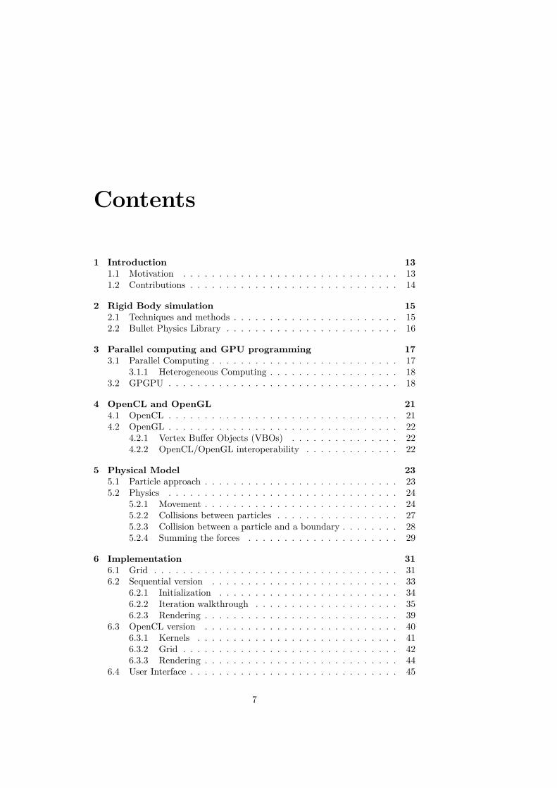
Contents

1 Introduction 131.1 Motivation . . . . . . . . . . . . . . . . . . . . . . . . . . . . . . 131.2 Contributions . . . . . . . . . . . . . . . . . . . . . . . . . . . . . 14

2 Rigid Body simulation 152.1 Techniques and methods . . . . . . . . . . . . . . . . . . . . . . . 152.2 Bullet Physics Library . . . . . . . . . . . . . . . . . . . . . . . . 16

3 Parallel computing and GPU programming 173.1 Parallel Computing . . . . . . . . . . . . . . . . . . . . . . . . . . 17

3.1.1 Heterogeneous Computing . . . . . . . . . . . . . . . . . . 183.2 GPGPU . . . . . . . . . . . . . . . . . . . . . . . . . . . . . . . . 18

4 OpenCL and OpenGL 214.1 OpenCL . . . . . . . . . . . . . . . . . . . . . . . . . . . . . . . . 214.2 OpenGL . . . . . . . . . . . . . . . . . . . . . . . . . . . . . . . . 22

4.2.1 Vertex Buffer Objects (VBOs) . . . . . . . . . . . . . . . 224.2.2 OpenCL/OpenGL interoperability . . . . . . . . . . . . . 22

5 Physical Model 235.1 Particle approach . . . . . . . . . . . . . . . . . . . . . . . . . . . 235.2 Physics . . . . . . . . . . . . . . . . . . . . . . . . . . . . . . . . 24

5.2.1 Movement . . . . . . . . . . . . . . . . . . . . . . . . . . . 245.2.2 Collisions between particles . . . . . . . . . . . . . . . . . 275.2.3 Collision between a particle and a boundary . . . . . . . . 285.2.4 Summing the forces . . . . . . . . . . . . . . . . . . . . . 29

6 Implementation 316.1 Grid . . . . . . . . . . . . . . . . . . . . . . . . . . . . . . . . . . 316.2 Sequential version . . . . . . . . . . . . . . . . . . . . . . . . . . 33

6.2.1 Initialization . . . . . . . . . . . . . . . . . . . . . . . . . 346.2.2 Iteration walkthrough . . . . . . . . . . . . . . . . . . . . 356.2.3 Rendering . . . . . . . . . . . . . . . . . . . . . . . . . . . 39

6.3 OpenCL version . . . . . . . . . . . . . . . . . . . . . . . . . . . 406.3.1 Kernels . . . . . . . . . . . . . . . . . . . . . . . . . . . . 416.3.2 Grid . . . . . . . . . . . . . . . . . . . . . . . . . . . . . . 426.3.3 Rendering . . . . . . . . . . . . . . . . . . . . . . . . . . . 44

6.4 User Interface . . . . . . . . . . . . . . . . . . . . . . . . . . . . . 45

7

7 Results 477.1 Behavior . . . . . . . . . . . . . . . . . . . . . . . . . . . . . . . . 477.2 Performance . . . . . . . . . . . . . . . . . . . . . . . . . . . . . . 53

7.2.1 Sequential CPU version . . . . . . . . . . . . . . . . . . . 537.2.2 OpenCL version . . . . . . . . . . . . . . . . . . . . . . . 54

7.3 Bullet Comparison . . . . . . . . . . . . . . . . . . . . . . . . . . 54

8 Conclusions 578.1 Summary . . . . . . . . . . . . . . . . . . . . . . . . . . . . . . . 578.2 Future work . . . . . . . . . . . . . . . . . . . . . . . . . . . . . . 58

A Source Code Samples 63A.1 Kernels . . . . . . . . . . . . . . . . . . . . . . . . . . . . . . . . 63

8

List of Figures

3.1 Development of Floating Point Operations per Second (FLOPS)in NVIDIA GPUs and Intel CPUs. [8] . . . . . . . . . . . . . . . 19

3.2 Distribution of transistors in a CPU and a GPU [8]. . . . . . . . 193.3 Development of Memory Bandwidth for NVIDIA GPUs and Intel

CPUs. [8] . . . . . . . . . . . . . . . . . . . . . . . . . . . . . . . 20

5.1 Cube with 27 internal particles . . . . . . . . . . . . . . . . . . . 245.2 Cube with zero rotation . . . . . . . . . . . . . . . . . . . . . . . 265.3 Collision between particles modeled by a spring . . . . . . . . . . 275.4 Three example boundaries and their normals . . . . . . . . . . . 29

6.1 Grid with cell size equal to twice the particle radius . . . . . . . 326.2 Grid with cell size equal to particle radius, with particles close . 326.3 Grid with cell size equal to particle radius, with particles far apart 336.4 Body and cube UML class diagram . . . . . . . . . . . . . . . . . 346.5 Particle UML class diagram . . . . . . . . . . . . . . . . . . . . . 356.6 Initial simulation state . . . . . . . . . . . . . . . . . . . . . . . . 366.7 Flowchart showing a simulation iteration . . . . . . . . . . . . . . 376.8 Two-dimensional arrays used to draw cubes, where s is the side

length of the cube . . . . . . . . . . . . . . . . . . . . . . . . . . 416.9 Cube wireframe with numbered vertices . . . . . . . . . . . . . . 426.10 OpenCL kernels performing a simulation iteration, with kernels

iterating over rigid bodies . . . . . . . . . . . . . . . . . . . . . . 436.11 OpenCL kernels performing a simulation iteration, with kernels

iterating over rigid bodies when necessary, but otherwise overparticles . . . . . . . . . . . . . . . . . . . . . . . . . . . . . . . . 44

6.12 The user can reset the simulation to one of these four differentsize towers. . . . . . . . . . . . . . . . . . . . . . . . . . . . . . . 45

6.13 The two different render options in our application . . . . . . . . 45

7.1 Four snapshots from a running simulation . . . . . . . . . . . . . 487.2 Particle cubes stacked on top of each other . . . . . . . . . . . . 497.3 Screenshot of simulation where cubes are stacked on top of each

other . . . . . . . . . . . . . . . . . . . . . . . . . . . . . . . . . . 507.4 Two particle cubes interlocked . . . . . . . . . . . . . . . . . . . . 517.5 Screenshot of simulation where two cubes are interlocked . . . . . 517.6 Screenshot of cubes colliding and clumping up at the grid border 52

9

7.7 Graph showing difference in performance between CPU and GPUfor 4 selected problem sizes . . . . . . . . . . . . . . . . . . . . . 54

7.8 Graph showing GPU speedup over CPU simulation at variousproblem sizes . . . . . . . . . . . . . . . . . . . . . . . . . . . . . 55

7.9 Screenshot of stacked cubes in Bullet rigid body simulation . . . 55

8.1 A banana is very well suited for particle representation. . . . . . 588.2 A desk is very poorly suited for particle representation. . . . . . 598.3 With friction, these 3 cubes will rest in the current position.

Without friction, the middle cube will slowly slide down and pushthe other 2 cubes to the side. . . . . . . . . . . . . . . . . . . . . 59

10

List of Tables

7.1 Parameters used for simulation performance testing . . . . . . . . 537.2 CPU performance for 4 selected problem sizes . . . . . . . . . . . 537.3 GPU performance for 4 selected problem sizes . . . . . . . . . . . 547.4 GPU speedup over CPU from test runs . . . . . . . . . . . . . . 547.5 Performance of Bullet rigid body simulation on CPU . . . . . . . 56

11

12

Chapter 1

Introduction

In this chapter we briefly explain what a rigid body simulation is, and ourmotivations for creating one. We also explain what contributions our workbrings to the field.

In simple terms, a rigid body simulation is a simulation of interacting objectsthat do not deform when they collide. In real life such objects do not exist,as all objects will deform when they collide with something. However, thisdeformation can be computationally expensive to calculate.

In some cases the deformation of an object is an important factor in the physicalbehavior of the object. In these cases rigid body simulation is not appropriate.Examples of an object like this is a piece of cloth, or jelly.

However, for many objects the deformation is very insignificant. When simulat-ing such objects it can be a good idea to simplify the simulation by assumingthat the objects cannot be deformed at all, in other words to do a rigid bodysimulation.

1.1 Motivation

One area where rigid body simulations is particularly useful is computer ani-mation. Even with sophisticated software, animation is often a long and workintensive process. While manually animating realistic physics for a couple ofobjects is no problem, animating thousands of them is. For such a task, sim-ulation is the only feasible option. Computer animation does not require therigid bodies to be simulated in real time. However, good performance is stillimportant. The simulation time will directly influence the productivity of theanimator. A fast simulation will allow him or her to discover problems faster,and allows for more experimenting for better results.

A second important area for rigid body simulations is video games. A com-mon trait for all rigid body simulation in video games is that they have to bereal-time. This effectively limits the complexity of the simulation to something

13

that looks and feels right, rather than being absolutely physically correct. How-ever, between different games, the requirement for complexity in the rigid bodysimulation can vary.

Sometimes the rigid body simulation can be important to the gameplay itself.An example of this could be an adventure game where you have to move objectsaround and jump on them to reach your goal. In other cases the rigid bodysimulation is only for visual effect. An example of this could be the fallingdebris from a destroyed unit in a strategy game. Clearly, the first examplerequires a more accurate rigid body simulation than the latter.

In this thesis we want to especially focus on the last example; simulations whichdo not require very fine accuracy. Instead we aim for these simulations to bevery fast, while at the same time look and feel correct.

1.2 Contributions

We provide a full open source implementation of a rigid body simulation, using aparticle method. The source code can be found at http://code.google.com/p/particle-rigid-body/. We combine techniques from different sources tocreate a fast and stable simulation. We accelerate our simulation with OpenCL,and show how OpenCL is well suited to this task.

14

Chapter 2

Rigid Body simulation

In this chapter we describe what a rigid body simulation entails, and presentsome of the existing techniques and methods available.

A rigid body simulation can be roughly divided into two parts, collision detec-tion and collision response [3]. The purpose of collision detection is to checkwhether the rigid bodies are in contact. If they are in contact, the simulationshould also at this point extract any information about the collision necessaryfor the next step, collision response. This information can vary depending onthe techniques used, but examples might be information such as intersectionpoints and penetration depths.

Collision response is about creating appropriate forces and impulses betweenthe colliding rigid bodies, to make the objects behave in accordance with thelaws of physics.

The computation time spent for each of these two parts is roughly equal, makingit important to be able to efficiently perform both.

2.1 Techniques and methods

Most collision detection algorithms use polyhedron representations for the rigidbodies. This means the bodies are made of vertices, edges and faces, just like therepresentation used by 3D graphics libraries such as OpenGL. Many algorithmsalso require that the bodies are convex. Fortunately, non-convex models canalways be split into a group of convex ones. One technique to do this is usingbinary space partitioning [9]. However, finding a minimal partitioning is NP-hard, and many partitioning methods often produce a large number of convexsmaller bodies, which is inefficient.

It is important for collision detection to limit the search somehow. Testing everysingle pair of objects for a possible collision is very computationally intensive.Considerable time can be saved by using a space partition. There are variousdifferent ways to do this, and some of the most notable are voxel grids, octrees,k-d trees and BSP trees [3].

15

Another technique to improve the performance of collision detection is to use abounding volume of the body, such as a sphere or box. Detecting collisions withthese shapes is a lot simpler and faster, however, they often do not provide agood approximation of the original shape.

The most accurate methods for collision response are the Finite Element Meth-ods. They work by decomposing the body into a large number of smaller ele-ments and then calculate the stress and strain on each of these smaller elements.However, these methods are computationally expensive and can not be used inreal-time simulations. They are fine for testing engineering structures, but cannot be used in interactive applications.

One of the most popular group of methods are Penalty Methods, largely becausethey are easily implemented. When two objects are found to be colliding, thesemethods use information about the collision to calculate an appropriate forcebetween them. A common example is the spring model, in which a spring forceis used to force contacting points apart.

A problem with these methods is that they often require tuning of several vari-ables to create realistic results, such as spring coefficients in the case of the springmodel. There is also little evidence to suggest that these methods accuratelysimulate what happens in real life. However, they can readily be applied whereaccuracy is not as important as simply getting realistic looking results.

Impulse-Based Methods model the forces between bodies through a series ofimpulses. An object resting on the ground will actually be vibrating up anddown in a tiny movement, due to repeated impulses from the ground.

2.2 Bullet Physics Library

Bullet Physics Library [1, 5] is an open source physics engine featuring collisiondetection, soft body and rigid body dynamics. The library is widely used forvideo games, movies and 3D modelling software. Examples of products that haveused Bullet include the video game Grand Theft Auto IV by Rockstar Games,the benchmarking utility 3D Mark 2011 by Futuremark, the Hollywood movie2012 by Sony Pictures Imageworks, and the 3D modelling tools Blender 3D andCinema 4D.

We have chosen to compare our results with the Bullet Physics Library be-cause it is free, open source, cross platform, and consequently in widespreaduse.

16

Chapter 3

Parallel computing andGPU programming

3.1 Parallel Computing

Parallel computing is a form of computation in which multiple calculations areperformed simultaneously. This is based on the principle that large problemscan often be divided into smaller problems, which can be solved concurrently,opposed to sequentially like traditional non-parallel computing.

The main driving force between the recent development into parallel computingcomes from the stagnation of the frequency of modern processors. The powerdensity in modern processors are approaching the limit of what silicon can han-dle with current cooling techniques. This is known as the power wall.

Parallel computing can be embodied in many different forms, many of whichdo not exclude each other. The following are some of the layers of parallelismexposed by modern hardware [4]:

Multi-chip parallelism This means having several physical processor chipsin a single computer. These chips share resources such as system memorythrough which the chips can relatively inexpensively communicate.

Multi-core parallelism This is similiar to multi-chip parallelism, with thedistinction that the cores are all contained in a single chip. This letsthe cores share resources like on-chip cache, allowing for less expensivecommunication.

Multi-context (thread) parallelism This is when a single core can switchbetween multiple execution contexts with little or no overhead.

Instruction parallelism This is when a single processor can execute morethan one instruction simultaneously.

Traditionally, floating-point operations were considered expensive, while mem-ory accesses were considered cheap. These roles have since been reversed, and

17

memory has become the limiting factor in most applications. Data has to betransferred through a limited number of pins at a limited frequency, causingwhat is known as the von Neumann bottleneck.

3.1.1 Heterogeneous Computing

Recent developments are also showing rising interests in heterogeneous com-puting. Heterogeneous computing refers to systems that use a combination ofdifferent types of computational units.

The motivation for using heterogeneous systems is that although problems canbe divided into smaller problems, all these smaller problems might not be of thesame nature, and might benefit from different hardware architectures.

In the past, advances in technology and frequency scaling allowed most appli-cations to increase in performance without structural changes. However, today,the effect of these advances are less dramatic since new obstacles such as thevon Neumann bottleneck and the power wall have been introduced. Brodtkorbet al. [4] mentions the combination of a Central Processing Unit (CPU) anda Graphics Processing Unit (GPU) as one of the most interesting examples ofheterogeneous systems for node level heterogeneous computing.

While neither the CPU or the GPU are heterogenous systems by themselves,they form a heterogeneous system when they are used together.

3.2 GPGPU

Using the GPU for computations traditionally handled by the CPU is known asGeneral Purpose computing on Graphics Processing Units (GPGPU). The GPUis a specialized accelerator, designed for the acceleration of graphics computa-tions. Their parallel nature allows them to efficiently perform large numbers offloating-point operations.

In terms of Floating Point Operations per Second (FLOPS), the GPU has hasfar surpassed the CPU, as can be seen in figure 3.1.

The reason for this huge discrepancy in floating-point capability is that the GPUis specialized for intensive, highly parallel computation, and is designed suchthat more transistors are devoted to data processing rather than flow controland data caching.

An illustration of the distribution of transistors in a CPU and a GPU can beseen in figure 3.2.

The GPU also has much higher memory bandwidth than the CPU, which canbe seen in figure 3.3.

These two factors make the GPU a very interesting platform for computationallyintense applications. A GPU can almost be seen as a small supercomputer,allowing a single computer to perform simulations that previously belonged tothe domain of larger clusters of computers.

18

Figure 3.1: Development of Floating Point Operations per Second (FLOPS) inNVIDIA GPUs and Intel CPUs. [8]

Figure 3.2: Distribution of transistors in a CPU and a GPU [8].

This has created ample new possibilities for the scientific community. Problemssuch as fluid simulation, molecular dynamics, medical imaging and many moreare experiencing drastic performance improvements. This can often mean thedifference between seeing the results of an operation almost immediately, asopposed to waiting for hours or even days.

However, a downside to using GPUs is that they typically use a PCI express bus,which can become a very serious bottleneck in cases where the entire problemdoes not fit in the GPUs memory. A second generation PCI express x16 busallows a theoretical maximum of 8 GB/s of data transfer between CPU andGPU memory.

Initially, GPUs were not designed for GPGPU. GPUs were programmed usingshaders, a set of software instructions performed on the GPU. These shadersare tightly knit to graphical concepts such as vertices and pixels. In order toperform operations that were not related to graphics, the problem had to be

19

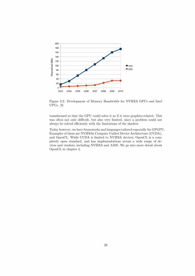
Figure 3.3: Development of Memory Bandwidth for NVIDIA GPUs and IntelCPUs. [8]

transformed so that the GPU could solve it as if it were graphics-related. Thiswas often not only difficult, but also very limited, since a problem could notalways be solved efficiently with the limitations of the shaders.

Today however, we have frameworks and languages tailored especially for GPGPU.Examples of these are NVIDIAs Compute Unified Device Architecture (CUDA),and OpenCL. While CUDA is limited to NVIDIA devices, OpenCL is a com-pletely open standard, and has implementations across a wide range of de-vices and vendors, including NVIDIA and AMD. We go into more detail aboutOpenCL in chapter 4.

20

Chapter 4

OpenCL and OpenGL

In this chapter we briefly describe two of the core technologies we are usingin our application. First we describe OpenCL, which we use to accelerate oursimulation on the GPU. Then we describe OpenGL, which we use to render oursimulation, and see how OpenCL and OpenGL can work together.

4.1 OpenCL

OpenCL (Open Computing Language) is a framework suited for parallel pro-gramming of heterogenous systems [12]. The framework includes the OpenCLC language, which is a language based on C99, for writing kernels, functionsthat execute on OpenCL devices such as a GPU.

An OpenCL device consists of multiple Compute Units, which in turn consistsof multiple Processing Elements. These correspond to the streaming multipro-cessors and scalar processors of a GPU respectively. When a kernel is to beexecuted it is put into a command queue, and then assigned to appropriatecompute units and processing elements.

OpenCL supports two different programming models. They are a Data Paral-lelÂămodel, and a Task parallel. In the data parallel model the same kernel isexecuted simultaneously across the compute units or processing elements. In thetask parallel model different kernels are executed. For our application we wantto use the data parallel model. This is because we will be simulating many ele-ments, and want to use the same kernel for every element. Filling the commandqueue with a kernel for each simulation element is very inefficient.

The data parallel kernel is divided into Work Items. A work item is the shareof the kernel executed by a single processing element. When enqueueing a dataparallel kernel the user has to specify the total number of work items the kernelshould have, and also how many of these work items should be given to eachcompute unit. The group of work items given to a compute unit is called aWorkgroup. The user has to take care to provide reasonable numbers, since thememory available in a compute unit is limited. The total number of work items

21

also needs to be divisible by the number of work items given to each computeunit, in other words the size of the workgroup.

4.2 OpenGL

OpenGL, short for Open Graphics Library, is a software interface to graphicshardware [10]. It is a 3D graphics and modeling library, which is very fast,and also very portable. OpenGL implementations can be found on all majorplatforms and operating systems, including of course Windows, Mac OS andLinux.

OpenGL is intended to be used with hardware designed and optimized for dis-playing and manipulating 3D graphics. Software-only implementations do ex-ist, however they generally do not perform as well, and may lack special ef-fects.

OpenGL is procedural rather than descriptive. What this means is that insteadof describing the scene and how it should look, the programmer instead writesstep by step the operations required to create the desired appearance. Thesesteps are calls to the many OpenCL functions which are used to draw graphicsprimitives such as points, lines and triangles in three dimensions.

OpenGL does not include any sort of window management, or user interac-tion. Each operating system has its own functions for this purpose and has theresponsibility of giving OpenGL the control to draw images in a window. How-ever there are cross platform libraries for this, such as GLUT (OpenGL utilitytoolkit) and SDL (Simple DirectMedia Layer).

4.2.1 Vertex Buffer Objects (VBOs)

A Vertex Buffer Object is an OpenGL extension that provides functions for up-loading graphics data, such as vertex positions, normal vectors, color values etc.,to a video device for non-immediate-mode rendering. Non-immediate-renderingbasically means that the graphical elements are not rendered immediately asthey are calculated. Instead the values are saved in a buffer on the device untilall elements in the buffer are ready to be rendered. Then they are all renderedat once. This offers better performance, primarily because the data is locatedin video device memory rather than ordinary system memory, which allows thedevice to render it directly.

4.2.2 OpenCL/OpenGL interoperability

When using OpenCL there is an even greater incentive for using VBOs. Sincecalculations are performed on the GPU there should no longer be necessary toupload the data to the VBO buffers from system memory. Indeed, OpenCLand OpenGL offers interoperability which allows VBO buffers to be read andwritten to directly by the OpenCL kernels.

22

Chapter 5

Physical Model

In the following sections we present the physical model we have chosen for ourimplementation and go through the physics equations that govern the movementand behavior of the rigid bodies. Our physical model is mostly based on thework of Takahiro Harada in the book GPU Gems 3 [7].

5.1 Particle approach

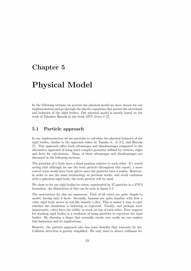
In our implementation we use particles to calculate the physical behavior of therigid bodies, similar to the approach taken by Tanaka et. al [11], and Harada[7]. This approach offers both advantages and disadvantages compared to thealternative approach of using more complex geometry defined by vertices, edgesand faces for calculations. Many of these advantages and disadvantages arediscussed in the following sections.

The particles of a body have a fixed position relative to each other. It’s worthnoting that although we use the term particle throughout this report, a morecorrect term would have been sphere since the particles have a radius. However,in order to use the same terminology as previous works, and avoid confusionwith a spherical rigid body, the term particle will be used.

We chose to let our rigid bodies be cubes, represented by 27 particles in a 3*3*3formation. An illustration of this can be seen in figure 5.1.

The motivations for this are numerous. First of all cubes are quite simple tomodel, having only 6 faces. Secondly, humans are quite familiar with how acubic rigid body moves in real life, namely a dice. This is makes it easy to spotwhether the simulation is behaving as expected. Finally, and perhaps mostimportantly, cubes have the ability to stack on top of each other. Poor supportfor stacking rigid bodies is a weakness of using particles to represent the rigidbodies. By choosing a shape that normally stacks very easily we can explorethis limitation and its implications.

However, the particle approach also has some benefits that warrants its use.Collision detection is greatly simplified. We only need to detect collisions be-

23

Figure 5.1: Cube with 27 internal particles

tween particles. Detecting a collision between to spheres is as simple as checkingwhether the distance between the center points is less than the sum of the ra-diuses of the spheres. The particle approach is also well suited for a GPU sinceit is easily parallelizable.

5.2 Physics

5.2.1 Movement

For the translation of a body, the following equations hold. When a force Facts on a rigid body, it gives the body impulse, which is change of the linearmomentum of the rigid body, P. In other words, the time derivative of P isequal to F:

dPdt

= F (5.1)

The definition of momentum is:

P = Mv (5.2)

where M is the mass of the rigid body, and v is its linear velocity. Through thisdefinition we can obtain the velocity as

24

v = PM

(5.3)

and, of course, velocity is the time derivative of the position x:

dxdt

= v (5.4)

The following equations govern the rotation of a rigid body. When a force actson a point of a rigid body that is different from the center of mass, it also givesthe rigid body torque. Torque is the rate of change of angular momentum L,like impulse is to linear momentum.

The amount of torque depends on the relative position r of the point where theforce acts compared to the center of mass. More specifically, torque τ is definedas the cross product of r and the acting force F.

dLdt

= τ = r× F (5.5)

The angular velocity w is obtained through the following equation:

w = I(t)−1L (5.6)

where I(t) is the inertia tensor of the rigid body at time t, and is a 3 ∗ 3 matrix,and I(t)−1 is its inverse. Inertia is a measure of an objects resistance to changeto its rotation, and the inertia tensor contains the objects inertia around all 3axes.

Inertia, and thus the inertia tensor, depends on the shape, size and mass of anobject. For a cuboid object, the inertia tensor looks like the following:

I =

112m(h2 + d2) 0 0

0 112m(w2 + d2) 0

0 0 112m(w2 + h2)

(5.7)

where h is the height, w is the width and d is the depth of the cuboid object.For a cube where height, width and depth are equal to the cube side s, theinertia tensor becomes:

I =

16ms

2 0 00 1

6ms2 0

0 0 16ms

2

(5.8)

Inverting this matrix yields the inverse inertia tensor used in equation 5.6:

I−1 =

6ms2 0 00 6

ms2 00 0 6

ms2

(5.9)

25

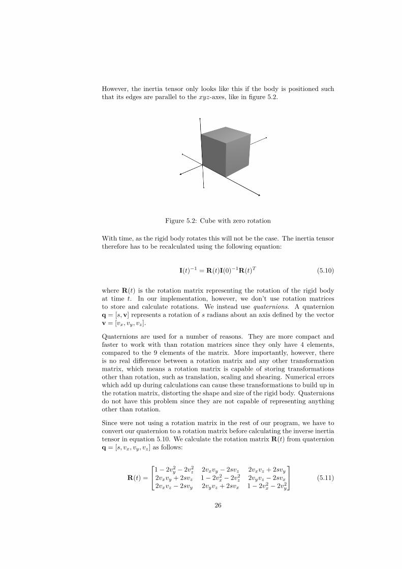
However, the inertia tensor only looks like this if the body is positioned suchthat its edges are parallel to the xyz-axes, like in figure 5.2.

Figure 5.2: Cube with zero rotation

With time, as the rigid body rotates this will not be the case. The inertia tensortherefore has to be recalculated using the following equation:

I(t)−1 = R(t)I(0)−1R(t)T (5.10)

where R(t) is the rotation matrix representing the rotation of the rigid bodyat time t. In our implementation, however, we don’t use rotation matricesto store and calculate rotations. We instead use quaternions. A quaternionq = [s,v] represents a rotation of s radians about an axis defined by the vectorv = [vx, vy, vz].

Quaternions are used for a number of reasons. They are more compact andfaster to work with than rotation matrices since they only have 4 elements,compared to the 9 elements of the matrix. More importantly, however, thereis no real difference between a rotation matrix and any other transformationmatrix, which means a rotation matrix is capable of storing transformationsother than rotation, such as translation, scaling and shearing. Numerical errorswhich add up during calculations can cause these transformations to build up inthe rotation matrix, distorting the shape and size of the rigid body. Quaternionsdo not have this problem since they are not capable of representing anythingother than rotation.

Since were not using a rotation matrix in the rest of our program, we have toconvert our quaternion to a rotation matrix before calculating the inverse inertiatensor in equation 5.10. We calculate the rotation matrix R(t) from quaternionq = [s, vx, vy, vz] as follows:

R(t) =

1− 2v2y − 2v2

z 2vxvy − 2svz 2vxvz + 2svy

2vxvy + 2svz 1− 2v2x − 2v2

z 2vyvz − 2svx

2vxvz − 2svy 2vyvz + 2svx 1− 2v2x − 2v2

y

(5.11)

26

We can then calculate the inverse inertia tensor at time t using equation 5.10,and then calculate the angular velocity w using equation 5.6. We then wantto use the angular velocity to update our rotation quaternion. The variationof quaternion q with angular velocity w is calculated using the following equa-tion:

dq =[cos(θ

2

),a sin

(θ

2

)](5.12)

where a = w|w| is the rotation axis and θ = |wdt| is the rotation angle. The

quaternion at time t+ dt is calculated by the following equation:

q(t+ dt) = dq × q(t) (5.13)

where the multiplication of two quaternions q0 = [s0,v0] and q1 = [s1,v1] isdefined as follows:

q0 × q1 = [s0s1 − v0 · v1, s0v1 + s1v0 + v0 × v1] (5.14)

5.2.2 Collisions between particles

With the movement of the rigid bodies in place, the next thing to consider isthe detection and reaction of collisions. As mentioned earlier, collision detectionbetween particles is trivial. We only need to check whether the distance betweentwo particles is less than the sum of their radiuses. In our implementation wesubtract a small number from this check to avoid particles within the same cubeto register a collision with each other. The particles within a cube are positionedperfectly close to each other, however numerical inaccuracies can cause this tobe detected as a collision.

When a collision occurs the particles are pushed away from each other by a forcemodeled by a linear spring, as illustrated in figure 5.3.

Figure 5.3: Collision between particles modeled by a spring

This force is calculated with the following equation:

27

fi,spring = −k (d− |rij |)rij

|rij |(5.15)

where k is the spring coefficient, d is the particle diameter, i is the index of theparticle on which the force is acting, jÂăis the index of the colliding particle,and rij is the relative position of particle j with respect to particle i.

In addition to this spring force, we add a damping force which opposes thevelocity of the particle. This force causes energy to dissipate and makes therigid bodies come to rest, rather than bouncing around forever.

This force is modeled by a dashpot and is calculated using the following equa-tion:

fi,damping = cvij (5.16)

where c is the damping coefficient, and vij is the relative velocity of particlejÂăwith respect to particle i.

To calculate this we need the velocities of the particles. The velocity of a particleis equal to the linear velocity of the rigid body it is a part of, plus the tangentialvelocity caused by the rotation of the rigid body.

We use the following equation to calculate the tangential velocity of a parti-cle:

vtangent = w×(

r−w · w · r|w2|

)(5.17)

where r is the particle position relative to the center of the rigid body, and wis the angular velocity of the body.

5.2.3 Collision between a particle and a boundary

Similar forces are applied at the boundaries of the domain to keep the rigidbodies inside. However, since the domain does not move, the equations can besimplified somewhat. The boundary spring forces are calculated individuallyfor each axis, since the force at a boundary only affects the force along the axiswhich is parallel to the normal of the boundary face, as seen in figure 5.4.

As an example, the equation for a particle colliding with the boundary whosenormal is along the x-axis, and will be pushing the particle in the negativedirection, looks like the following:

fi,boundary−springx= k(lx − px − r) (5.18)

where lx is the boundary position on the x-axis, px is the particle position onthe x-axis, r is the particle radius, and the expression inside the parentheses isthe position of the colliding point of the particle with respect to the boundary.We don’t have a minus in front of k in this equation because we multiply with

28

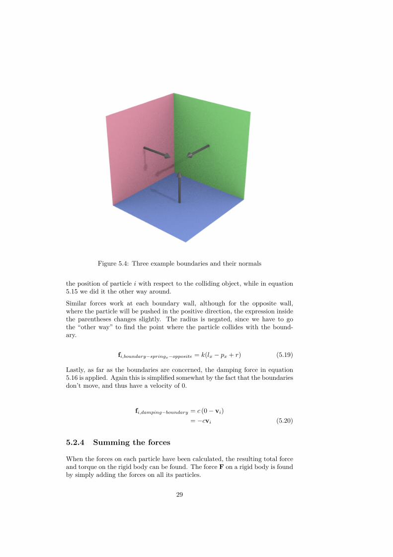
Figure 5.4: Three example boundaries and their normals

the position of particle i with respect to the colliding object, while in equation5.15 we did it the other way around.

Similar forces work at each boundary wall, although for the opposite wall,where the particle will be pushed in the positive direction, the expression insidethe parentheses changes slightly. The radius is negated, since we have to gothe “other way” to find the point where the particle collides with the bound-ary.

fi,boundary−springx−opposite = k(lx − px + r) (5.19)

Lastly, as far as the boundaries are concerned, the damping force in equation5.16 is applied. Again this is simplified somewhat by the fact that the boundariesdon’t move, and thus have a velocity of 0.

fi,damping−boundary = c (0− vi)= −cvi (5.20)

5.2.4 Summing the forces

When the forces on each particle have been calculated, the resulting total forceand torque on the rigid body can be found. The force F on a rigid body is foundby simply adding the forces on all its particles.

29

F =∑

i∈RigidBody

fi (5.21)

where fi is the total force acting on particle i. The torque T on a rigid bodyis calculated by summing the cross product of the relative position of a particleto the center of the rigid body and the total force on the particle:

T =∑

i∈RigidBody

(ri × fi) (5.22)

where ri is the position of particle i relative to the center of the rigid body.

30

Chapter 6

Implementation

We have implemented a rigid body simulation in C++ and OpenCL. In thelast chapter we presented the physical model, and the equations that govern thebehavior of our implementation. In this chapter we describe how these equationscome together to create a rigid body simulation. We begin by describing thesequential version written in C++. We then describe the OpenCL version, howit has been modified compared to the C++ version, and what considerationsaffected this process.

However, first of all we describe a grid structure we use in our application whichgreatly improves the time complexity of the simulation. This is vital for beingable to simulate a large number of rigid bodies in real time.

6.1 Grid

Naively checking every other particle in the simulation when detecting collisionsdoes not scale very well. In fact it carries a time complexity of O(n2). In orderto improve this we implement a grid structure described in the paper ParticleSimulation using CUDA by Simon Green [6].

The simulation world is divided into a uniform grid, and at the beginning ofevery iteration we check the position of every particle in order to determinewhich grid cell it belongs to. We find the cell index i = (ix, iy, iz) with thefollowing equation [7]:

i = (p−min)d

(6.1)

where p is the position of the particle, and min is the position of the gridcorner with the smallest coordinates in all dimensions. In our case the leftmost,backmost, lower corner. Finally, d is the cell size (cell side length).

By setting the grid cell size equal to twice that of the particle radius, we knowthat a cell will hold a maximum of 4 particles [6]. We also know that in order

31

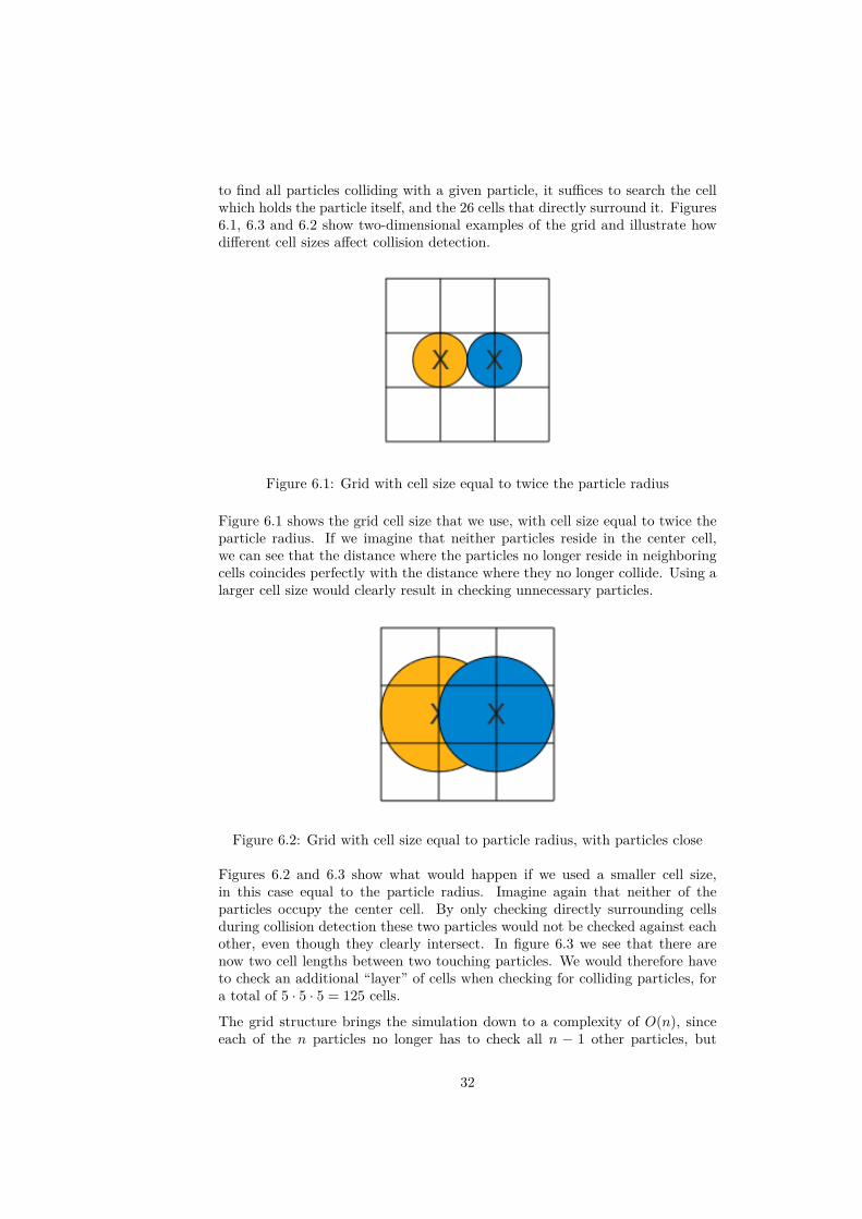
to find all particles colliding with a given particle, it suffices to search the cellwhich holds the particle itself, and the 26 cells that directly surround it. Figures6.1, 6.3 and 6.2 show two-dimensional examples of the grid and illustrate howdifferent cell sizes affect collision detection.

Figure 6.1: Grid with cell size equal to twice the particle radius

Figure 6.1 shows the grid cell size that we use, with cell size equal to twice theparticle radius. If we imagine that neither particles reside in the center cell,we can see that the distance where the particles no longer reside in neighboringcells coincides perfectly with the distance where they no longer collide. Using alarger cell size would clearly result in checking unnecessary particles.

Figure 6.2: Grid with cell size equal to particle radius, with particles close

Figures 6.2 and 6.3 show what would happen if we used a smaller cell size,in this case equal to the particle radius. Imagine again that neither of theparticles occupy the center cell. By only checking directly surrounding cellsduring collision detection these two particles would not be checked against eachother, even though they clearly intersect. In figure 6.3 we see that there arenow two cell lengths between two touching particles. We would therefore haveto check an additional “layer” of cells when checking for colliding particles, fora total of 5 · 5 · 5 = 125 cells.

The grid structure brings the simulation down to a complexity of O(n), sinceeach of the n particles no longer has to check all n − 1 other particles, but

32

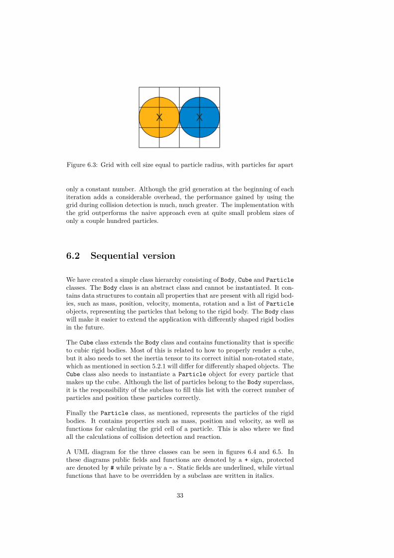
Figure 6.3: Grid with cell size equal to particle radius, with particles far apart

only a constant number. Although the grid generation at the beginning of eachiteration adds a considerable overhead, the performance gained by using thegrid during collision detection is much, much greater. The implementation withthe grid outperforms the naive approach even at quite small problem sizes ofonly a couple hundred particles.

6.2 Sequential version

We have created a simple class hierarchy consisting of Body, Cube and Particleclasses. The Body class is an abstract class and cannot be instantiated. It con-tains data structures to contain all properties that are present with all rigid bod-ies, such as mass, position, velocity, momenta, rotation and a list of Particleobjects, representing the particles that belong to the rigid body. The Body classwill make it easier to extend the application with differently shaped rigid bodiesin the future.

The Cube class extends the Body class and contains functionality that is specificto cubic rigid bodies. Most of this is related to how to properly render a cube,but it also needs to set the inertia tensor to its correct initial non-rotated state,which as mentioned in section 5.2.1 will differ for differently shaped objects. TheCube class also needs to instantiate a Particle object for every particle thatmakes up the cube. Although the list of particles belong to the Body superclass,it is the responsibility of the subclass to fill this list with the correct number ofparticles and position these particles correctly.

Finally the Particle class, as mentioned, represents the particles of the rigidbodies. It contains properties such as mass, position and velocity, as well asfunctions for calculating the grid cell of a particle. This is also where we findall the calculations of collision detection and reaction.

A UML diagram for the three classes can be seen in figures 6.4 and 6.5. Inthese diagrams public fields and functions are denoted by a + sign, protectedare denoted by # while private by a -. Static fields are underlined, while virtualfunctions that have to be overridden by a subclass are written in italics.

33

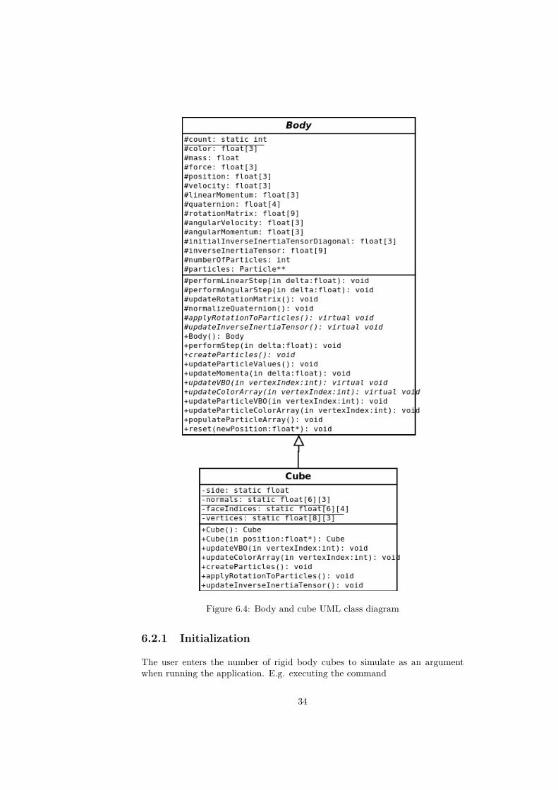
Figure 6.4: Body and cube UML class diagram

6.2.1 Initialization

The user enters the number of rigid body cubes to simulate as an argumentwhen running the application. E.g. executing the command

34

Figure 6.5: Particle UML class diagram

./rigidbody 1000

will launch a simulation of 1,000 cubes, which corresponds to 27,000 particles.The first thing that happens is that Cube objects representing these cubes areinstantiated, as well as Particle objects for their particles. Static counters areused to keep track of how many cubes and particles have been created at alltimes. This information is used to fill global arrays that hold references to everycube, and every particle. This is needed to iterate over all cubes and particleslater. As they are created, we place the cubes above each other while movingthem back and forth between 4 different positions along the ground plane. Ascreenshot of the resulting initial position for the cubes can be seen in figure6.6.

The reason for this is simply to create interesting behavior. The cubes are movedonly so much that their sides and corners still slightly overlap, causing inevitablerotation when they collide with each other at the ground. We use a randomnumber generator to generate colors for the rigid bodies. Since this has nosignificant importance for the simulation other than visuals the standard C++rand function is good enough for this. However, we seed the random numbergenerator with a timestamp to avoid generating the same color combinationsevery time the application is executed.

6.2.2 Iteration walkthrough

In this section we walk through all the calculations that are performed in aniteration. A flowchart showing a quick overview of an iteration can be seen in

35

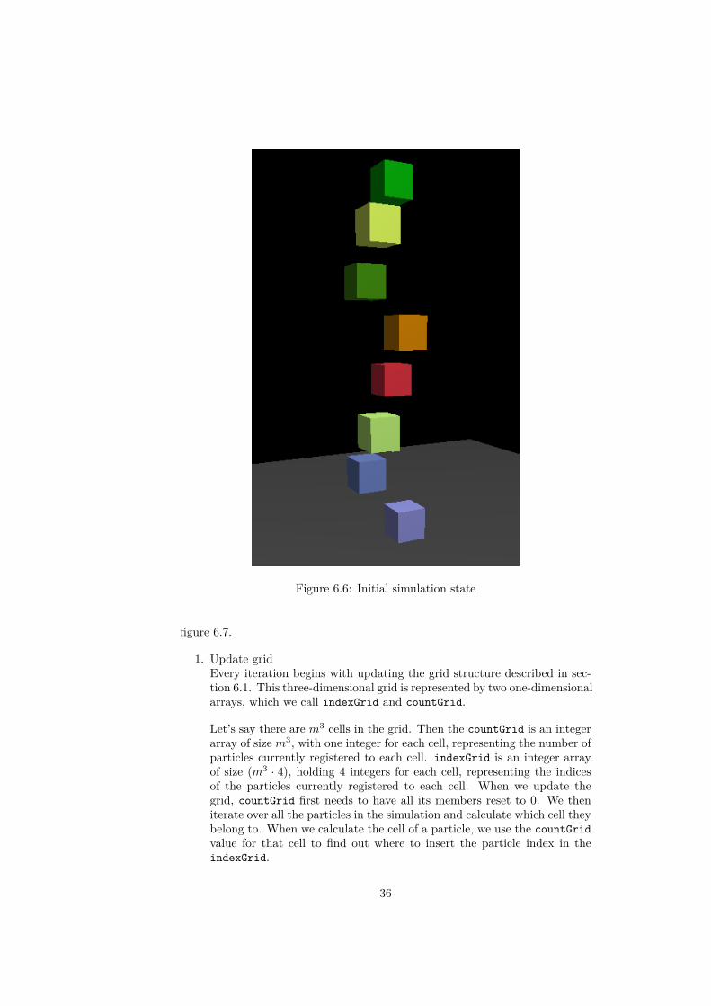
Figure 6.6: Initial simulation state

figure 6.7.

1. Update gridEvery iteration begins with updating the grid structure described in sec-tion 6.1. This three-dimensional grid is represented by two one-dimensionalarrays, which we call indexGrid and countGrid.

Let’s say there are m3 cells in the grid. Then the countGrid is an integerarray of size m3, with one integer for each cell, representing the number ofparticles currently registered to each cell. indexGrid is an integer arrayof size (m3 · 4), holding 4 integers for each cell, representing the indicesof the particles currently registered to each cell. When we update thegrid, countGrid first needs to have all its members reset to 0. We theniterate over all the particles in the simulation and calculate which cell theybelong to. When we calculate the cell of a particle, we use the countGridvalue for that cell to find out where to insert the particle index in theindexGrid.

36

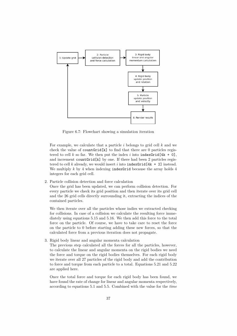
Figure 6.7: Flowchart showing a simulation iteration

For example, we calculate that a particle i belongs to grid cell k and wecheck the value of countGrid[k] to find that there are 0 particles regis-tered to cell k so far. We then put the index i into indexGrid[4k + 0],and increment countGrid[k] by one. If there had been 2 particles regis-tered to cell k already, we would insert i into indexGrid[4k + 2] instead.We multiply k by 4 when indexing indexGrid because the array holds 4integers for each grid cell.

2. Particle collision detection and force calculationOnce the grid has been updated, we can perform collision detection. Forevery particle we check its grid position and then iterate over its grid celland the 26 grid cells directly surrounding it, extracting the indices of thecontained particles.

We then iterate over all the particles whose indies we extracted checkingfor collisions. In case of a collision we calculate the resulting force imme-diately using equations 5.15 and 5.16. We then add this force to the totalforce on the particle. Of course, we have to take care to reset the forceon the particle to 0 before starting adding these new forces, so that thecalculated force from a previous iteration does not propagate.

3. Rigid body linear and angular momenta calculationThe previous step calculated all the forces for all the particles, however,to calculate the linear and angular momenta on the rigid bodies we needthe force and torque on the rigid bodies themselves. For each rigid bodywe iterate over all 27 particles of the rigid body and add the contributionto force and torque from each particle to a total. Equations 5.21 and 5.22are applied here.

Once the total force and torque for each rigid body has been found, wehave found the rate of change for linear and angular momenta respectively,according to equations 5.1 and 5.5. Combined with the value for the time

37

delta, ∆t, (which is defined by the user) we can then update the linearand angular momenta by P← P + F ·∆t and L← L + τ ·∆t.

However, before we move on we check whether the absolute value of thelinear momentum in each direction is greater than a maximum valuecalculated from a user defined terminal momentum. If it is, we set itto the maximum value, or negative the maximum value, depending onwhether the momentum is positive or negative. This is called a clampoperation. In this case we clamp the momentum between the range[−maximum momentum,maximum momentum]. We do this to preventthe rigid bodies from accelerating to unrealistically great speeds whenthey fall for a long time. This is similar to how in real life air resistancewould prevent objects from accelerating past a terminal velocity, howeverour approach is a little simplified. Air resistance would build up as thevelocity of the object increased, slowing acceleration gradually. Our ap-proach allows the object to accelerate unhindered up until it hits terminalvelocity, upon which time acceleration halts completely.

4. Rigid body position and rotation updateOnce we have the linear and angular momenta we can find the linear andangular velocities of the rigid bodies. We iterate over all the rigid bodies inthe simulation and for each we calculate their linear and angular velocityas follows. Finding the linear velocity is easily done simply by dividingthe linear momentum by the mass of the rigid body, in accordance withequation 5.3. Finding the angular velocity is a more extensive operation.

To calculate the angular velocity we need to update the inverse inertiatensor for the objects current rotation. To calculate the inverse inertiatensor we need the rotation matrix for the objects current rotation. Butas mentioned in section 5.2.1 we use quaternions to represent rotation.Therefore we first have to convert our quaternion to a rotation matrixusing equation 5.11. However, equation 5.11 requires that the quaternionq is normalized, meaning that |q| = 1. We check whether |q| is more thana small threshold unequal to 1. If it is, we normalize it as if it were anyother vector: q← q

|q| . We can then calculate the new inverse inertia tensorusing equation 5.10, and consequently we can find the angular velocitywith equation 5.6.

We have the velocities of the rigid body and can update the position.There are many possible ways to do this, using different numerical inte-gration methods. In this implementation we simply use Euler method,and update position x by x← x + v ·∆t. We update rotation using equa-tion 5.13. Using a more advanced integration method could be a part offuture work, explored in more detail in section 8.2.

5. Particle position and velocity updateWe now have everything we need to update the positions and velocitiesof the particles. This operation could technically be performed at thebeginning of the iteration instead of at the end. The particles would thenreceive the changes from the previous iteration at the beginning of thenext, which would be fine if we only rendered the cube geometry. However,we have added the ability to render the particles themselves instead of the

38

cubes for the purpose of visually demonstrating how the simulation works.If we did not update the particles before rendering there would be a singleframe of delay of the visualized particles compared to their computation.This is minuscule of course, especially at small time steps, but there is nodownside to updating the particles at the end of the iteration instead, sowe might as well do so.

To calculate the position of a particle we need the current position androtation of the rigid body it belongs to, as well as the initial position of theparticle relative to the center of the rigid body at zero rotation. It is theresponsibility of the rigid body subclass to convey these initial positions tothe particles when updating their current positions. We therefore iterateover all rigid bodies, and for each rigid body iterate over their particleswhen performing this operation. The new particle position is found byapplying the rotation to the initial relative position and adding the rigidbody position. We apply the rotation by multiplying the initial relativeposition vector by the rotation matrix, yielding a new position vector. Wethen add the rigid body position vector to this.

We update the particle velocity by applying equation 5.17, which is straightforward to calculate tangential velocity, and then adding the linear veloc-ity of the rigid body itself. The only thing to consider is that we mustcheck whether the angular velocity is zero before dividing by the square ofits size. This would of course would also be zero, causing an error due todivision by zero. If the angular division turns out to be zero, the tangen-tial velocity is simply zero also. However the linear velocity of the rigidbody is still added.

6. Render resultsWhen all the calculations of an iteration are completed, we need to renderthe results to the screen. For rendering we use OpenGL and vertex bufferobjects (VBOs) explained in section 4.2. We use two separate VBOs inour implementation. One for rendering cubes, and one for rendering par-ticles. We go into more detail about rendering in section 6.2.3. For now,suffice to say that we update only the VBO for the currently chosen ob-ject representation. If complete cubes are chosen the vertex positions andnormals have to be recalculated using their original position and the cur-rent rotation. If particles are chosen we already have the vertex positions,since these are simply the particle positions, and we only need to insertthese values into the VBO. Once the VBO values have been updated weneed to copy them to the device, before we draw the chosen VBO to thescreen.

6.2.3 Rendering

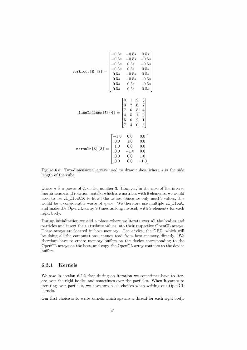
We use three two-dimensional arrays when drawing cubes. We call them normals,faceIndices and vertices. We present these arrays as matrices in figure 6.8.To help make sense of these arrays we have figure 6.9 which shows a wireframecube with numbered vertices.

The vertices array contains the positions of the vertices themselves. There are

39

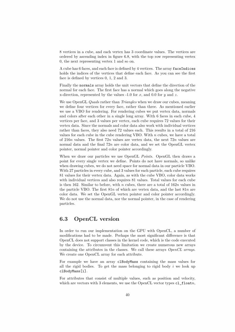
8 vertices in a cube, and each vertex has 3 coordinate values. The vertices areordered by ascending index in figure 6.8, with the top row representing vertex0, the next representing vertex 1 and so on.

A cube has 6 faces, and each face is defined by 4 vertices. The array faceIndicesholds the indices of the vertices that define each face. As you can see the firstface is defined by vertices 0, 1, 2 and 3.

Finally the normals array holds the unit vectors that define the direction of thenormal for each face. The first face has a normal which goes along the negativex-direction, represented by the values -1.0 for x, and 0.0 for y and z.

We use OpenGL Quads rather than Triangles when we draw our cubes, meaningwe define four vertices for every face, rather than three. As mentioned earlierwe use a VBO for rendering. For rendering cubes we put vertex data, normalsand colors after each other in a single long array. With 6 faces in each cube, 4vertices per face, and 3 values per vertex, each cube requires 72 values for theirvertex data. Since the normals and color data also work with individual verticesrather than faces, they also need 72 values each. This results in a total of 216values for each cube in the cube rendering VBO. With n cubes, we have a totalof 216n values. The first 72n values are vertex data, the next 72n values arenormal data and the final 72n are color data, and we set the OpenGL vertexpointer, normal pointer and color pointer accordingly.

When we draw our particles we use OpenGL Points. OpenGL then draws apoint for every single vertex we define. Points do not have normals, so unlikewhen drawing cubes, we do not need space for normal data in our particle VBO.With 27 particles in every cube, and 3 values for each particle, each cube requires81 values for their vertex data. Again, as with the cube VBO, color data workswith individual vertices and also requires 81 values. Total values for each cubeis then 162. Similar to before, with n cubes, there are a total of 162n values inthe particle VBO. The first 81n of which are vertex data, and the last 81n arecolor data. We set the OpenGL vertex pointer and color pointer accordingly.We do not use the normal data, nor the normal pointer, in the case of renderingparticles.

6.3 OpenCL version

In order to run our implementation on the GPU with OpenCL, a number ofmodifications had to be made. Perhaps the most significant difference is thatOpenCL does not support classes in the kernel code, which is the code executedby the device. To circumvent this limitation we create numerous new arrayscontaining the attributes in the classes. We call these arrays OpenCL arrays.We create one OpenCL array for each attribute.

For example we have an array clBodyMass containing the mass values forall the rigid bodies. To get the mass belonging to rigid body i we look upclBodyMass[i].

For attributes that consist of multiple values, such as position and velocity,which are vectors with 3 elements, we use the OpenCL vector types cl_floatn,

40

vertices[8][3] =

−0.5s −0.5s 0.5s−0.5s −0.5s −0.5s−0.5s 0.5s −0.5s−0.5s 0.5s 0.5s0.5s −0.5s 0.5s0.5s −0.5s −0.5s0.5s 0.5s −0.5s0.5s 0.5s 0.5s

faceIndices[6][4] =

0 1 2 33 2 6 77 6 5 44 5 1 05 6 2 17 4 0 3

normals[6][3] =

−1.0 0.0 0.00.0 1.0 0.01.0 0.0 0.00.0 −1.0 0.00.0 0.0 1.00.0 0.0 −1.0

Figure 6.8: Two-dimensional arrays used to draw cubes, where s is the sidelength of the cube

where n is a power of 2, or the number 3. However, in the case of the inverseinertia tensor and rotation matrix, which are matrices with 9 elements, we wouldneed to use cl_float16 to fit all the values. Since we only need 9 values, thiswould be a considerable waste of space. We therefore use multiple cl_float,and make the OpenCL array 9 times as long instead, with 9 elements for eachrigid body.

During initialization we add a phase where we iterate over all the bodies andparticles and insert their attribute values into their respective OpenCL arrays.These arrays are located in host memory. The device, the GPU, which willbe doing all the computations, cannot read from host memory directly. Wetherefore have to create memory buffers on the device corresponding to theOpenCL arrays on the host, and copy the OpenCL array contents to the devicebuffers.

6.3.1 Kernels

We saw in section 6.2.2 that during an iteration we sometimes have to iter-ate over the rigid bodies and sometimes over the particles. When it comes toiterating over particles, we have two basic choices when writing our OpenCLkernels.

Our first choice is to write kernels which spawns a thread for each rigid body.

41

Figure 6.9: Cube wireframe with numbered vertices

In this case each thread has to iterate over all the particles of their respectiverigid bodies during the iteration phases that require iteration over all particles.This results in a fewer amount of more computationally expensive kernels. Also,the iteration over particles drastically increases the number of memory accessesperformed by the kernel, potentially decreasing performance.

An illustration of the resulting kernels and which parts of an iteration theycomplete can be seen in figure 6.10

Our second choice is to create kernels which spawn threads for each rigid bodywhen required, but otherwise use kernels which spawn threads for each particle.This results in a larger quantity of kernels, however each kernel is less com-putationally expensive. An illustration of the resulting kernels and how theycomplete the iteration can be seen in figure 6.11.

We tried both approaches in our implementation, and discovered that the sec-ond approach, i.e. the one illustrated in figure 6.11, performed better in allcircumstances, and will be the approach used in any further discussion aboutthe implementation.

6.3.2 Grid

As can be seen in figures 6.10 and 6.11, the operation of updating the grid usestwo kernels. One for resetting the grid and one for updating it. The first, whichwe call the resetGrid kernel spawn a thread for each grid cell, while the second,

42

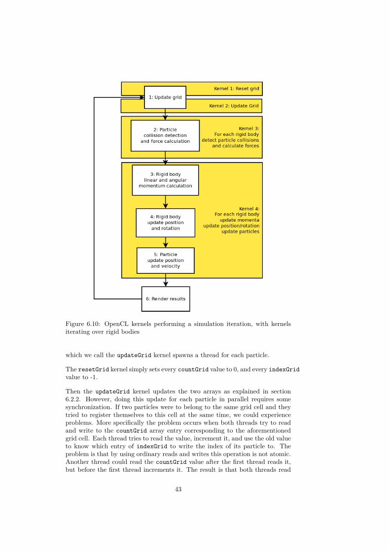
Figure 6.10: OpenCL kernels performing a simulation iteration, with kernelsiterating over rigid bodies

which we call the updateGrid kernel spawns a thread for each particle.

The resetGrid kernel simply sets every countGrid value to 0, and every indexGridvalue to -1.

Then the updateGrid kernel updates the two arrays as explained in section6.2.2. However, doing this update for each particle in parallel requires somesynchronization. If two particles were to belong to the same grid cell and theytried to register themselves to this cell at the same time, we could experienceproblems. More specifically the problem occurs when both threads try to readand write to the countGrid array entry corresponding to the aforementionedgrid cell. Each thread tries to read the value, increment it, and use the old valueto know which entry of indexGrid to write the index of its particle to. Theproblem is that by using ordinary reads and writes this operation is not atomic.Another thread could read the countGrid value after the first thread reads it,but before the first thread increments it. The result is that both threads read

43

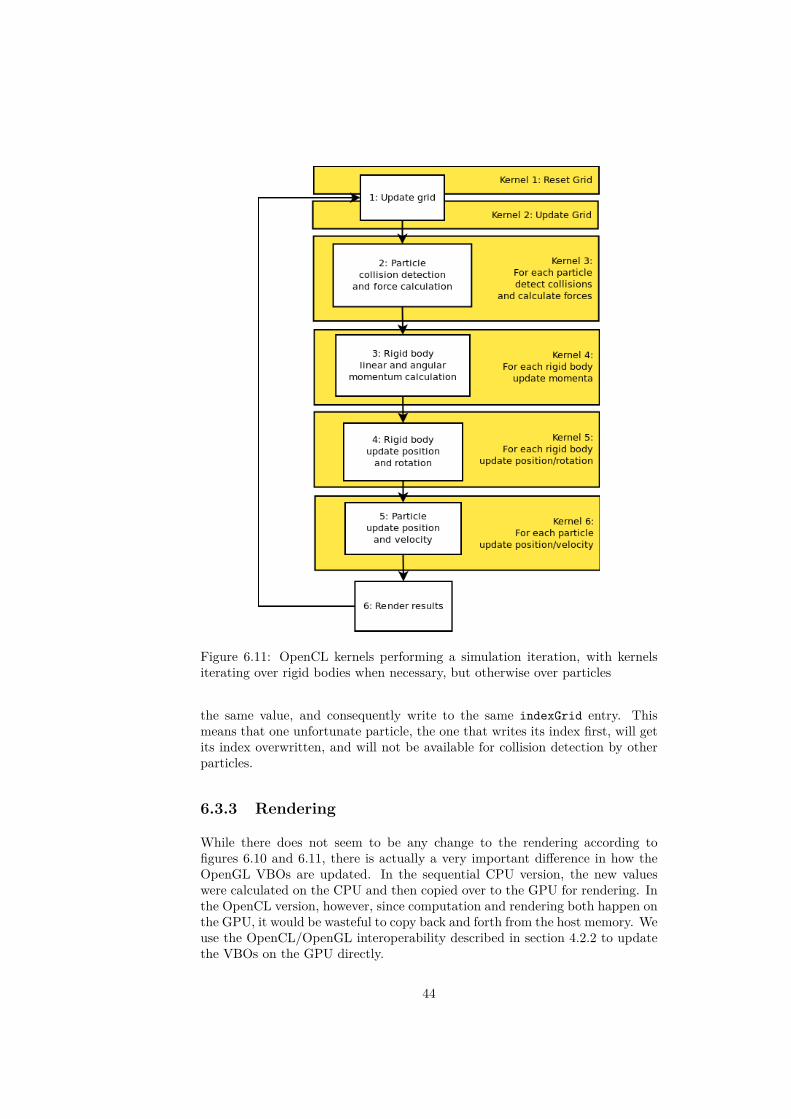
Figure 6.11: OpenCL kernels performing a simulation iteration, with kernelsiterating over rigid bodies when necessary, but otherwise over particles

the same value, and consequently write to the same indexGrid entry. Thismeans that one unfortunate particle, the one that writes its index first, will getits index overwritten, and will not be available for collision detection by otherparticles.

6.3.3 Rendering

While there does not seem to be any change to the rendering according tofigures 6.10 and 6.11, there is actually a very important difference in how theOpenGL VBOs are updated. In the sequential CPU version, the new valueswere calculated on the CPU and then copied over to the GPU for rendering. Inthe OpenCL version, however, since computation and rendering both happen onthe GPU, it would be wasteful to copy back and forth from the host memory. Weuse the OpenCL/OpenGL interoperability described in section 4.2.2 to updatethe VBOs on the GPU directly.

44

Using the kernels in figure 6.11 we update the VBO for rendering cubes in kernel5, while we update the VBO for rendering particles in kernel 6.

The final render stage is then only comprised of correctly setting vertex, colorand normal pointers, and drawing the VBO arrays.

6.4 User Interface

We have created a simple user interface for our simulation using freeglut, anopen source alternative to GLUT, the OpenGL Utility Toolkit [2].

The interface we have created allows us to spin around the scene and zoom inand out using the mouse. We have also added functionality for resetting thesimulation without having to restart the application. By pressing the numbers1 through 5 on the keyboard, the simulation is reset to one of five differentformations. One of these is the formation shown in figure 6.6. The other optionsare to place the cubes in towers of various sizes. An image of these towers canbe seen in figure 6.12.

Figure 6.12: The user can reset the simulation to one of these four different sizetowers.

By pressing the letter P on the keyboard the user switches between renderingparticles and cubes. A screenshot of the two different rendering options can beseen in figure 6.13.

Figure 6.13: The two different render options in our application

45

46

Chapter 7

Results

In this chapter we present and discuss the results from our application. In thefirst section we focus on the behavior of the simulation. We explore some of thestrengths and weaknesses of the choices we have made.

Next we take a look at the performance of our application, and especially howthe OpenCL version performs compared to the CPU version.

Finally we compare our results to the Bullet Physics Library.

7.1 Behavior

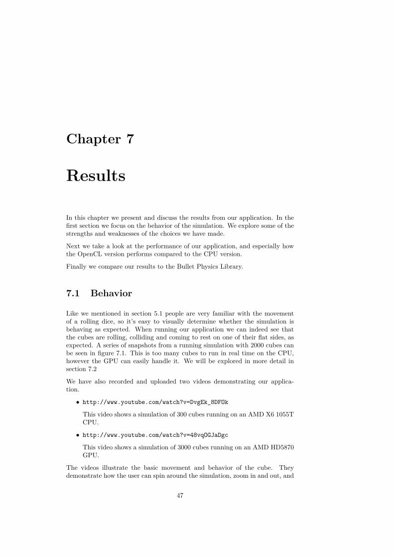
Like we mentioned in section 5.1 people are very familiar with the movementof a rolling dice, so it’s easy to visually determine whether the simulation isbehaving as expected. When running our application we can indeed see thatthe cubes are rolling, colliding and coming to rest on one of their flat sides, asexpected. A series of snapshots from a running simulation with 2000 cubes canbe seen in figure 7.1. This is too many cubes to run in real time on the CPU,however the GPU can easily handle it. We will be explored in more detail insection 7.2

We have also recorded and uploaded two videos demonstrating our applica-tion.

• http://www.youtube.com/watch?v=DvgEk_8DFOk

This video shows a simulation of 300 cubes running on an AMD X6 1055TCPU.

• http://www.youtube.com/watch?v=48vqOGJaDgc

This video shows a simulation of 3000 cubes running on an AMD HD5870GPU.

The videos illustrate the basic movement and behavior of the cube. Theydemonstrate how the user can spin around the simulation, zoom in and out, and

47

Figure 7.1: Four snapshots from a running simulation

reset the simulation to several different starting positions. They also demon-strate how the user can switch between the two different rendering methods,rendering cubes, and rendering particles.

The videos also show how the cubes are unable to stay stacked in a large tower,causing a collapse. In the rest of this section we will explore this issue, as wellas some other problems with our simulation.

Let us first begin with the inability to stack properly. We mentioned this alreadyin section 5.1, and it was indeed one of the reasons for choosing cubic rigid bodiesfor our simulation.

The inability to stack is caused by a combination of factors. We think onefactor is the way forces are modeled between particles. Since they are modeledby a spring, stacking multiple cubes on top of each other is like creating a longvertical spring. This will inevitably become unstable, especially when the cubesare not placed perfectly straight on top of each other. This brings us over toanother factor, which is probably the most influential one and has to do withthe particle approach itself. Since the cubes are made out of particles, theirsides are not completely flat, and when cubes rest on top of each other they willslide into the grooves created by the spherical particles. An illustration of thiscan be seen in figure 7.2.

An example of how this looks in the application itself when rendering cubes canbe seen in figure 7.3.

Needless to say, this is not ideal behavior, and is one of the prices that has to

48

Figure 7.2: Particle cubes stacked on top of each other

be paid when using this particle approach.

Another problem we discovered with the particle approach was that the particlecubes could get interlocked with each other. An illustration of how this happenscan be seen in figure 7.4, and an example of how it looks in the simulation canbe seen in the screenshot in figure 7.5. Although not visible in these pictures,the biggest problem with this scenario is actually not the interlocking itself, butrather the erratic movement exercised by the interlocked bodies. This is causedby the fact that there is not enough room for the entire between the particlesin the other rigid body. The particle will be pushed back and forth, and thatsame force will affect the rigid body.

The best way to fix this problem would be to prevent the interlocking fromoccuring in the first place. One way to do this is to limit the mass or speed ofthe rigid bodies. The rigid bodies need a certain amount of momentum in orderfor their particles to force their way into another rigid body. However, this isnot an ideal solution since we would like to be able to simulate bodies of any

49

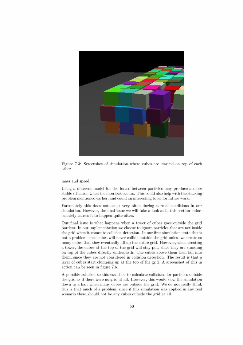
Figure 7.3: Screenshot of simulation where cubes are stacked on top of eachother

mass and speed.

Using a different model for the forces between particles may produce a morestable situation when the interlock occurs. This could also help with the stackingproblem mentioned earlier, and could an interesting topic for future work.

Fortunately this does not occur very often during normal conditions in oursimulation. However, the final issue we will take a look at in this section unfor-tunately causes it to happen quite often.

Our final issue is what happens when a tower of cubes goes outside the gridborders. In our implementation we choose to ignore particles that are not insidethe grid when it comes to collision detection. In our first simulation state this isnot a problem since cubes will never collide outside the grid unless we create somany cubes that they eventually fill up the entire grid. However, when creatinga tower, the cubes at the top of the grid will stay put, since they are standingon top of the cubes directly underneath. The cubes above them then fall intothem, since they are not considered in collision detection. The result is that alayer of cubes start clumping up at the top of the grid. A screenshot of this inaction can be seen in figure 7.6.

A possible solution to this could be to calculate collisions for particles outsidethe grid as if there were no grid at all. However, this would slow the simulationdown to a halt when many cubes are outside the grid. We do not really thinkthis is that much of a problem, since if this simulation was applied in any realscenario there should not be any cubes outside the grid at all.

50

Figure 7.4: Two particle cubes interlocked

Figure 7.5: Screenshot of simulation where two cubes are interlocked

51

Figure 7.6: Screenshot of cubes colliding and clumping up at the grid border

52

7.2 Performance

To measure performance we use timer functions included in GLUT. One of thefunctions allows us to get the time elapsed since the application started. Weget this time at the beginning of a frame, and then again at the end of a frame.The difference tells us how long this particular frame lasted. We then add thistime to a sum of frame times. Every 50 frames we use this sum to calculate theaverage framerate, or FPS (frames per second), during the time used by those50 frames. For the performance measurements in this section, we wait until allcubes are inside the grid, and then calculate an average FPS from ten of these50 frame intervals.

Our implementation provides a stable simulation when the timestep is set to0.01s. In order for the simulation to be real-time it needs to render 100 framesper second.

All the tests were run on a computer with an AMD X6 1055T CPU, 4 GB ofRAM, an AMD Radeon HD 5870 graphics card with Catalyst 10.12 drivers, andrunning Ubuntu Linux 10.10 32-bit.

The parameters used in the test simulation can be seen in table 7.1. Theseparameters create a nice and stable simulation.

Table 7.1: Parameters used for simulation performance testingParameter name Value

worldSize 15.0springCoefficient 100.0

dampingCoefficient 0.5timeDelta 0.01

particleRadius 0.20terminalVelocity 20.0

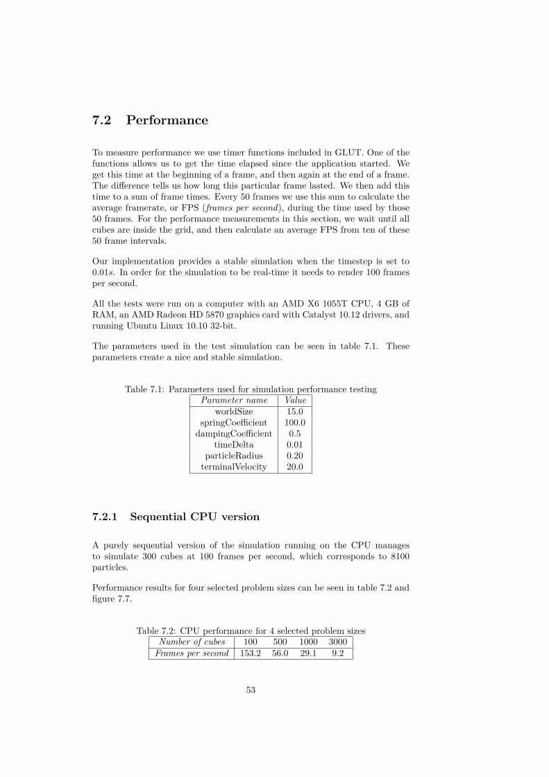
7.2.1 Sequential CPU version

A purely sequential version of the simulation running on the CPU managesto simulate 300 cubes at 100 frames per second, which corresponds to 8100particles.

Performance results for four selected problem sizes can be seen in table 7.2 andfigure 7.7.

Table 7.2: CPU performance for 4 selected problem sizesNumber of cubes 100 500 1000 3000

Frames per second 153.2 56.0 29.1 9.2

53

7.2.2 OpenCL version

The OpenCL version running on an AMD Radeon HD5870 manages to simulate3300 cubes at 100 frames per second. This corresponds to a total of 89100particles.

Performance results for four selected problem sizes can be seen in table 7.3 andfigure 7.7

Table 7.3: GPU performance for 4 selected problem sizesNumber of cubes 100 500 1000 3000

Frames per second 571.4 377.8 253.3 110.5

Figure 7.7: Graph showing difference in performance between CPU and GPUfor 4 selected problem sizes

The GPU speedup over CPU from these test runs can be seen in table 7.4 andfigure 7.8.

Table 7.4: GPU speedup over CPU from test runsNumber of cubes 100 500 1000 3000

Speedup 3.7 6.7 8.7 12.0

As expected we can see that the speedup rises as the problem size increases,which is in accordance with Gustafson’s law.

7.3 Bullet Comparison

We have also implemented a variation of our application which uses the BulletPhysics Library to perform the rigid body simulation. All other parts of theapplication such as rendering and user interface remain the same. The firstthing to notice about the Bullet simulation is that it uses the actual geometryof the cubes, and thus provides a more accurate simulation than our own. It

54

Figure 7.8: Graph showing GPU speedup over CPU simulation at various prob-lem sizes

also supports stacking cubes far better, as can be seen in the screenshot in figure7.9.

Figure 7.9: Screenshot of stacked cubes in Bullet rigid body simulation

Since the behavour of the Bullet simulation is better than our simulation, oursimulation should hopefully at least have better performance.

We test the performance of the Bullet simulation the same way we did our own,and compare the results. One thing we quickly discover is that the performanceof the Bullet simulation greatly increases once the rigid bodies settle down andstop moving. This is likely the result of some sort of optimization performed byBullet. When we measure the performance of the Bullet simulation we therefore

55

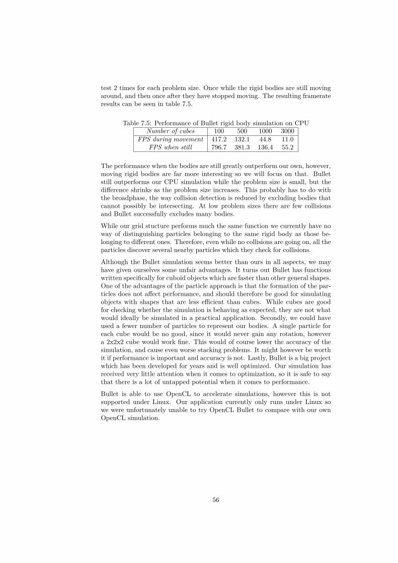
test 2 times for each problem size. Once while the rigid bodies are still movingaround, and then once after they have stopped moving. The resulting framerateresults can be seen in table 7.5.

Table 7.5: Performance of Bullet rigid body simulation on CPUNumber of cubes 100 500 1000 3000

FPS during movement 417.2 132.1 44.8 11.0FPS when still 796.7 381.3 136.4 55.2

The performance when the bodies are still greatly outperform our own, however,moving rigid bodies are far more interesting so we will focus on that. Bulletstill outperforms our CPU simulation while the problem size is small, but thedifference shrinks as the problem size increases. This probably has to do withthe broadphase, the way collision detection is reduced by excluding bodies thatcannot possibly be intersecting. At low problem sizes there are few collisionsand Bullet successfully excludes many bodies.

While our grid stucture performs much the same function we currently have noway of distinguishing particles belonging to the same rigid body as those be-longing to different ones. Therefore, even while no collisions are going on, all theparticles discover several nearby particles which they check for collisions.

Although the Bullet simulation seems better than ours in all aspects, we mayhave given ourselves some unfair advantages. It turns out Bullet has functionswritten specifically for cuboid objects which are faster than other general shapes.One of the advantages of the particle approach is that the formation of the par-ticles does not affect performance, and should therefore be good for simulatingobjects with shapes that are less efficient than cubes. While cubes are goodfor checking whether the simulation is behaving as expected, they are not whatwould ideally be simulated in a practical application. Secondly, we could haveused a fewer number of particles to represent our bodies. A single particle foreach cube would be no good, since it would never gain any rotation, howevera 2x2x2 cube would work fine. This would of course lower the accuracy of thesimulation, and cause even worse stacking problems. It might however be worthit if performance is important and accuracy is not. Lastly, Bullet is a big projectwhich has been developed for years and is well optimized. Our simulation hasreceived very little attention when it comes to optimization, so it is safe to saythat there is a lot of untapped potential when it comes to performance.

Bullet is able to use OpenCL to accelerate simulations, however this is notsupported under Linux. Our application currently only runs under Linux sowe were unfortunately unable to try OpenCL Bullet to compare with our ownOpenCL simulation.

56

Chapter 8

Conclusions

In this chapter we summarize what we have accomplished and what we havelearned from it. We also discuss how the work could be improved by futurework.

8.1 Summary

We have implemented a rigid body simulation using a particle approach in thehope of achieving high performance. We have shown that our simulation behaveswell, with the exception of some acceptable expected problems. We discoveredthat the performance of our simulation running on a CPU is comparable to thatof the Bullet Physics Engine for larger problem sizes. And, last but not least,we have managed to accelerate our simulation by up to a factor of 12 by portingit to OpenCL and running it on a GPU.

We believe the methods we have used for our rigid body simulation could beapplied well to visual elements in video games that do not affect the gameplayitself. Such elements do not require a lot of accuracy, but it is important thatthey look and feel correct. Certain objects are better suited for the approachthan others however. Using fewer particles to represent an object will result ina faster simulation. Therefore, objects that can be represented by few particleswhile still be able to largely retain their behavior are best. The objects shouldalso not be able to stack easily, since stacking is not well supported by theparticle approach.

Well suited objects tend to be rounded, and not too thin. An example of a verywell suited object can be seen in figure 8.1.

An example of an object which is very poorly suited to the particle approachcan be seen in figure 8.2.

This object, a desk, requires a lot of particles, which results in sub-optimal per-formance. The biggest problem is still that a desk should be able to have thingsplaced on top of it, which is poorly supported by the particle method.

57

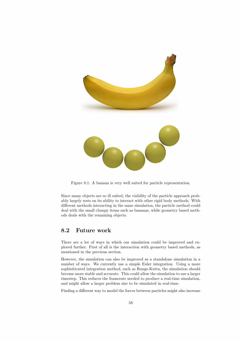
Figure 8.1: A banana is very well suited for particle representation.

Since many objects are so ill suited, the viability of the particle approach prob-ably largely rests on its ability to interact with other rigid body methods. Withdifferent methods interacting in the same simulation, the particle method coulddeal with the small clumpy items such as bananas, while geometry based meth-ods deals with the remaining objects.

8.2 Future work

There are a lot of ways in which our simulation could be improved and ex-plored further. First of all is the interaction with geometry based methods, asmentioned in the previous section.

However, the simulation can also be improved as a standalone simulation in anumber of ways. We currently use a simple Euler integration. Using a moresophisiticated integration method, such as Runge-Kutta, the simulation shouldbecome more stable and accurate. This could allow the simulation to use a largertimestep. This reduces the framerate needed to produce a real-time simulation,and might allow a larger problem size to be simulated in real-time.

Finding a different way to model the forces between particles might also increase

58

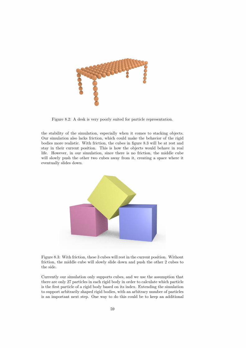
Figure 8.2: A desk is very poorly suited for particle representation.

the stability of the simulation, especially when it comes to stacking objects.Our simulation also lacks friction, which could make the behavior of the rigidbodies more realistic. With friction, the cubes in figure 8.3 will be at rest andstay in their current position. This is how the objects would behave in reallife. However, in our simulation, since there is no friction, the middle cubewill slowly push the other two cubes away from it, creating a space where iteventually slides down.

Figure 8.3: With friction, these 3 cubes will rest in the current position. Withoutfriction, the middle cube will slowly slide down and push the other 2 cubes tothe side.

Currently our simulation only supports cubes, and we use the assumption thatthere are only 27 particles in each rigid body in order to calculate which particleis the first particle of a rigid body based on its index. Extending the simulationto support arbitrarily shaped rigid bodies, with an arbitrary number of particlesis an important next step. One way to do this could be to keep an additional

59

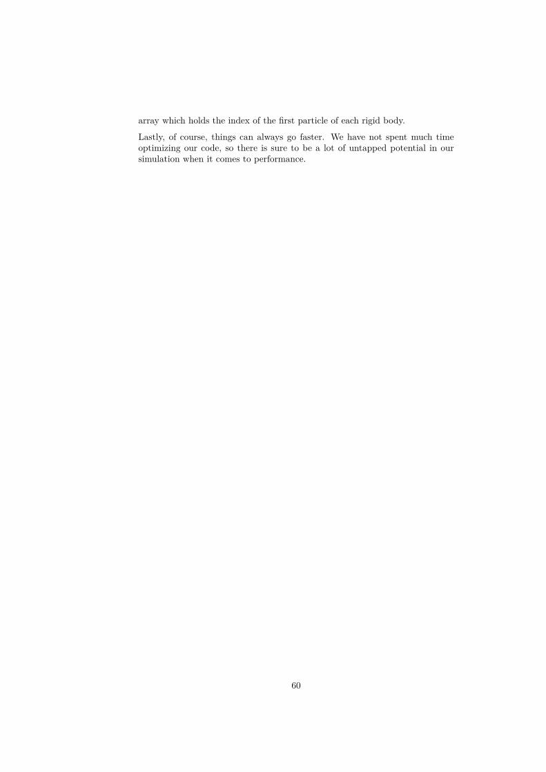
array which holds the index of the first particle of each rigid body.

Lastly, of course, things can always go faster. We have not spent much timeoptimizing our code, so there is sure to be a lot of untapped potential in oursimulation when it comes to performance.

60

Bibliography

[1] Bullet physics library. URL http://www.bulletphysics.org/.

[2] freeglut. URL http://freeglut.sourceforge.net/.

[3] Rahil Baber. Rigid body simulation. Master’s thesis, University of War-wick, 2006.

[4] Andre R. Brodtkorb, Christopher Dyken, Trond R. Hagen, Jon M.Hjelmervik, and Olaf O. Storaasli. State-of-the-art in heterogeneous com-puting. Scientific Programming, 18:1 – 33, 2010.

[5] Erwin Coumans. Bullet 2.76 Physics SDK Manual, 2010.

[6] Simon Green. Particle Simulation using CUDA. NVIDIA, May 2010.

[7] Takahiro Harada. Real-Time Rigid Body Simulation on GPUs, chapter 29.Addison-Wesley, 2007.

[8] NVIDIA CUDA C Programming Guide. NVIDIA, 3.2 edition, September2010.

[9] M. Paterson and F. F. Yao. Efficient binary space partitions for hidden-surface removal and solid modeling. Discrete and Computational Geometry,5:485 – 503, 1990.

[10] Jr. Richard S. Wright, Nicholas Haemel, Graham Sellers, and BenjaminLipchak. OpenGL SuperBible. Addison-Wesley, fifth edition, November2010.

[11] Masayuki Tanaka, Mikio Sakai, Ishikawajima-Harima, and SeiichiKoshizuka. Rigid body simulation using a particle method. ACM SIG-GRAPH 2006 Research posters, 2006.

[12] Ryoji Tsuchiyama, Takashi Nakamura, Takuro Iizuka, Akihiro Asahara,Satoshi Miki, and Satoru Tagawa. The OpenCL Programming Book. Fixs-tars Corporation, first edition, April 2010.

61

62

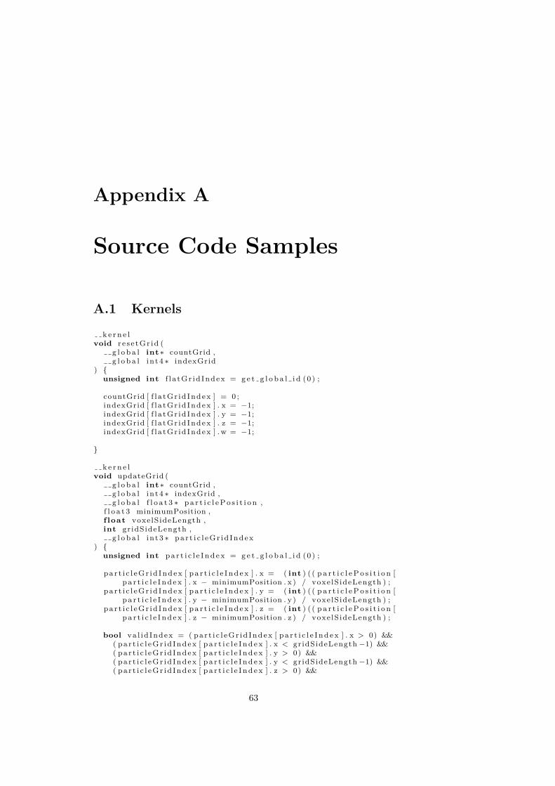
Appendix A

Source Code Samples

A.1 Kernels

k e r n e lvoid r e s e t G r i d (

g l o b a l int∗ countGrid ,g l o b a l i n t 4 ∗ indexGrid

) {unsigned int f l a t G r i d I n d e x = g e t g l o b a l i d (0 ) ;

countGrid [ f l a t G r i d I n d e x ] = 0 ;indexGrid [ f l a t G r i d I n d e x ] . x = −1;indexGrid [ f l a t G r i d I n d e x ] . y = −1;indexGrid [ f l a t G r i d I n d e x ] . z = −1;indexGrid [ f l a t G r i d I n d e x ] . w = −1;

}

k e r n e lvoid updateGrid (

g l o b a l int∗ countGrid ,g l o b a l i n t 4 ∗ indexGrid ,g l o b a l f l o a t 3 ∗ p a r t i c l e P o s i t i o n ,

f l o a t 3 minimumPosition ,f loat voxelSideLength ,int gr idSideLength ,

g l o b a l i n t 3 ∗ p a r t i c l e G r i d I n d e x) {

unsigned int p a r t i c l e I n d e x = g e t g l o b a l i d (0 ) ;

p a r t i c l e G r i d I n d e x [ p a r t i c l e I n d e x ] . x = ( int ) ( ( p a r t i c l e P o s i t i o n [p a r t i c l e I n d e x ] . x − minimumPosition . x ) / voxe lS ideLength ) ;

p a r t i c l e G r i d I n d e x [ p a r t i c l e I n d e x ] . y = ( int ) ( ( p a r t i c l e P o s i t i o n [p a r t i c l e I n d e x ] . y − minimumPosition . y ) / voxe lS ideLength ) ;

p a r t i c l e G r i d I n d e x [ p a r t i c l e I n d e x ] . z = ( int ) ( ( p a r t i c l e P o s i t i o n [p a r t i c l e I n d e x ] . z − minimumPosition . z ) / voxe lS ideLength ) ;

bool va l id Index = ( p a r t i c l e G r i d I n d e x [ p a r t i c l e I n d e x ] . x > 0) &&( p a r t i c l e G r i d I n d e x [ p a r t i c l e I n d e x ] . x < gr idSideLength −1) &&( p a r t i c l e G r i d I n d e x [ p a r t i c l e I n d e x ] . y > 0) &&( p a r t i c l e G r i d I n d e x [ p a r t i c l e I n d e x ] . y < gr idSideLength −1) &&( p a r t i c l e G r i d I n d e x [ p a r t i c l e I n d e x ] . z > 0) &&

63

( p a r t i c l e G r i d I n d e x [ p a r t i c l e I n d e x ] . z < gr idSideLength −1) ;

i f ( va l id Index ) {int x S t r i d e = gr idS ideLength ∗ gr idSideLength ;int y S t r i d e = gr idS ideLength ;int f l a t G r i d I n d e x = p a r t i c l e G r i d I n d e x [ p a r t i c l e I n d e x ] . x∗ x S t r i d e

+p a r t i c l e G r i d I n d e x [ p a r t i c l e I n d e x ] . y ∗ y S t r i d e +p a r t i c l e G r i d I n d e x [ p a r t i c l e I n d e x ] . z ;

int p a r t i c l e s I n C e l l = atomic inc (&countGrid [ f l a t G r i d I n d e x ] ) ;

i f ( p a r t i c l e s I n C e l l == 3) {indexGrid [ f l a t G r i d I n d e x ] . w = p a r t i c l e I n d e x ;

} else i f ( p a r t i c l e s I n C e l l == 2) {indexGrid [ f l a t G r i d I n d e x ] . z = p a r t i c l e I n d e x ;

} else i f ( p a r t i c l e s I n C e l l == 1) {indexGrid [ f l a t G r i d I n d e x ] . y = p a r t i c l e I n d e x ;

} else i f ( p a r t i c l e s I n C e l l == 0) {indexGrid [ f l a t G r i d I n d e x ] . x = p a r t i c l e I n d e x ;

}}

}

k e r n e lvoid c o l l i s i o n D e t e c t i o n (

g l o b a l f l o a t 3 ∗ part i c l eMass ,g l o b a l f l o a t 3 ∗ p a r t i c l e P o s i t i o n ,g l o b a l f l o a t 3 ∗ p a r t i c l e V e l o c i t y ,g l o b a l f l o a t 3 ∗ p a r t i c l e F o r c e ,

f loat par t i c l eRad iu s ,f loat worldSize ,f loat s p r i n g C o e f f i c i e n t ,f loat dampingCoef f i c i ent ,

g l o b a l i n t 3 ∗ par t i c l eGr id Index ,g l o b a l int∗ countGrid ,g l o b a l i n t 4 ∗ indexGrid ,

int gr idSideLength) {

unsigned int p a r t i c l e I n d e x = g e t g l o b a l i d (0 ) ;

p a r t i c l e F o r c e [ p a r t i c l e I n d e x ] . x = 0 .0 f ;p a r t i c l e F o r c e [ p a r t i c l e I n d e x ] . y = 0 .0 f ;p a r t i c l e F o r c e [ p a r t i c l e I n d e x ] . z = 0 .0 f ;

i n t 3 gr id Index = p a r t i c l e G r i d I n d e x [ p a r t i c l e I n d e x ] ;

// Pretend border c e l l i s 1 p o s i t i o n inwards to avoid check ingo u t s i d e bounds f o r ne ighbors

gr id Index = clamp ( gr idIndex , 1 , gr idSideLength −2) ;

int x S t r i d e = gr idS ideLength ∗ gr idSideLength ;int y S t r i d e = gr idS ideLength ;

int f l a t G r i d I n d e x = gr idIndex . x ∗ x S t r i d e +gr idIndex . y ∗ y S t r i d e + gr idIndex . z ;

i n t 4 n e i g h b o r C e l l s [ 2 7 ] ;int c e l l I n d e x J = 0 ;

64

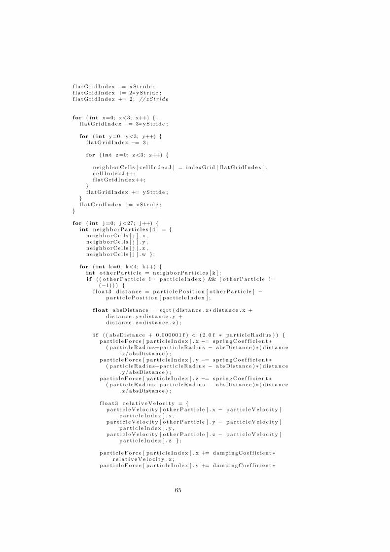
f l a t G r i d I n d e x −= x S tr i d e ;f l a t G r i d I n d e x += 2∗ y S t r i d e ;f l a t G r i d I n d e x += 2 ; // z S t r i d e

for ( int x=0; x<3; x++) {f l a t G r i d I n d e x −= 3∗ y S t r i d e ;

for ( int y=0; y<3; y++) {f l a t G r i d I n d e x −= 3 ;

for ( int z =0; z <3; z++) {

n e i g h b o r C e l l s [ c e l l I n d e x J ] = indexGrid [ f l a t G r i d I n d e x ] ;c e l l I n d e x J ++;f l a t G r i d I n d e x++;

}f l a t G r i d I n d e x += y St r i d e ;

}f l a t G r i d I n d e x += x St r i d e ;

}

for ( int j =0; j <27; j++) {int n e i g h b o r P a r t i c l e s [ 4 ] = {

n e i g h b o r C e l l s [ j ] . x ,n e i g h b o r C e l l s [ j ] . y ,n e i g h b o r C e l l s [ j ] . z ,n e i g h b o r C e l l s [ j ] . w } ;

for ( int k=0; k<4; k++) {int o t h e r P a r t i c l e = n e i g h b o r P a r t i c l e s [ k ] ;i f ( ( o t h e r P a r t i c l e != p a r t i c l e I n d e x ) && ( o t h e r P a r t i c l e !=

(−1) ) ) {f l o a t 3 d i s t a n c e = p a r t i c l e P o s i t i o n [ o t h e r P a r t i c l e ] −

p a r t i c l e P o s i t i o n [ p a r t i c l e I n d e x ] ;

f loat absDistance = s q r t ( d i s t a n c e . x∗ d i s t a n c e . x +d i s t a n c e . y∗ d i s t a n c e . y +d i s t a n c e . z∗ d i s t a n c e . z ) ;

i f ( ( absDistance + 0.000001 f ) < ( 2 . 0 f ∗ p a r t i c l e R a d i u s ) ) {p a r t i c l e F o r c e [ p a r t i c l e I n d e x ] . x −= s p r i n g C o e f f i c i e n t ∗

( p a r t i c l e R a d i u s+p a r t i c l e R a d i u s − absDistance ) ∗( d i s t a n c e. x/ absDistance ) ;

p a r t i c l e F o r c e [ p a r t i c l e I n d e x ] . y −= s p r i n g C o e f f i c i e n t ∗( p a r t i c l e R a d i u s+p a r t i c l e R a d i u s − absDistance ) ∗( d i s t a n c e

. y/ absDistance ) ;p a r t i c l e F o r c e [ p a r t i c l e I n d e x ] . z −= s p r i n g C o e f f i c i e n t ∗

( p a r t i c l e R a d i u s+p a r t i c l e R a d i u s − absDistance ) ∗( d i s t a n c e. z/ absDistance ) ;

f l o a t 3 r e l a t i v e V e l o c i t y = {p a r t i c l e V e l o c i t y [ o t h e r P a r t i c l e ] . x − p a r t i c l e V e l o c i t y [

p a r t i c l e I n d e x ] . x ,p a r t i c l e V e l o c i t y [ o t h e r P a r t i c l e ] . y − p a r t i c l e V e l o c i t y [

p a r t i c l e I n d e x ] . y ,p a r t i c l e V e l o c i t y [ o t h e r P a r t i c l e ] . z − p a r t i c l e V e l o c i t y [

p a r t i c l e I n d e x ] . z } ;

p a r t i c l e F o r c e [ p a r t i c l e I n d e x ] . x += dampingCoe f f i c i ent ∗r e l a t i v e V e l o c i t y . x ;

p a r t i c l e F o r c e [ p a r t i c l e I n d e x ] . y += dampingCoe f f i c i ent ∗

65

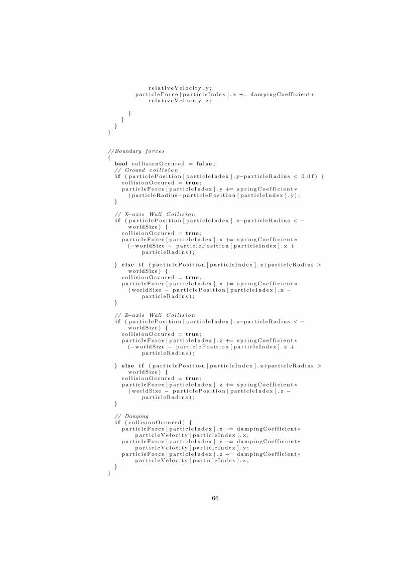
r e l a t i v e V e l o c i t y . y ;p a r t i c l e F o r c e [ p a r t i c l e I n d e x ] . z += dampingCoe f f i c i ent ∗

r e l a t i v e V e l o c i t y . z ;

}}

}}

//Boundary f o r c e s{

bool c o l l i s i o n O c c u r e d = fa l se ;// Ground c o l l i s i o ni f ( p a r t i c l e P o s i t i o n [ p a r t i c l e I n d e x ] . y−p a r t i c l e R a d i u s < 0 .0 f ) {

c o l l i s i o n O c c u r e d = true ;p a r t i c l e F o r c e [ p a r t i c l e I n d e x ] . y += s p r i n g C o e f f i c i e n t ∗

( pa r t i c l eRad iu s−p a r t i c l e P o s i t i o n [ p a r t i c l e I n d e x ] . y ) ;}

// X−a x i s Wall C o l l i s i o ni f ( p a r t i c l e P o s i t i o n [ p a r t i c l e I n d e x ] . x−p a r t i c l e R a d i u s < −

wor ldS ize ) {c o l l i s i o n O c c u r e d = true ;p a r t i c l e F o r c e [ p a r t i c l e I n d e x ] . x += s p r i n g C o e f f i c i e n t ∗

(−wor ldS ize − p a r t i c l e P o s i t i o n [ p a r t i c l e I n d e x ] . x +p a r t i c l e R a d i u s ) ;

} else i f ( p a r t i c l e P o s i t i o n [ p a r t i c l e I n d e x ] . x+p a r t i c l e R a d i u s >wor ldS ize ) {

c o l l i s i o n O c c u r e d = true ;p a r t i c l e F o r c e [ p a r t i c l e I n d e x ] . x += s p r i n g C o e f f i c i e n t ∗

( wor ldS ize − p a r t i c l e P o s i t i o n [ p a r t i c l e I n d e x ] . x −p a r t i c l e R a d i u s ) ;

}

// Z−a x i s Wall C o l l i s i o ni f ( p a r t i c l e P o s i t i o n [ p a r t i c l e I n d e x ] . z−p a r t i c l e R a d i u s < −

wor ldS ize ) {c o l l i s i o n O c c u r e d = true ;p a r t i c l e F o r c e [ p a r t i c l e I n d e x ] . z += s p r i n g C o e f f i c i e n t ∗

(−wor ldS ize − p a r t i c l e P o s i t i o n [ p a r t i c l e I n d e x ] . z +p a r t i c l e R a d i u s ) ;

} else i f ( p a r t i c l e P o s i t i o n [ p a r t i c l e I n d e x ] . z+p a r t i c l e R a d i u s >wor ldS ize ) {

c o l l i s i o n O c c u r e d = true ;p a r t i c l e F o r c e [ p a r t i c l e I n d e x ] . z += s p r i n g C o e f f i c i e n t ∗

( wor ldS ize − p a r t i c l e P o s i t i o n [ p a r t i c l e I n d e x ] . z −p a r t i c l e R a d i u s ) ;

}

// Dampingi f ( c o l l i s i o n O c c u r e d ) {

p a r t i c l e F o r c e [ p a r t i c l e I n d e x ] . x −= dampingCoe f f i c i ent ∗p a r t i c l e V e l o c i t y [ p a r t i c l e I n d e x ] . x ;

p a r t i c l e F o r c e [ p a r t i c l e I n d e x ] . y −= dampingCoe f f i c i ent ∗p a r t i c l e V e l o c i t y [ p a r t i c l e I n d e x ] . y ;

p a r t i c l e F o r c e [ p a r t i c l e I n d e x ] . z −= dampingCoe f f i c i ent ∗p a r t i c l e V e l o c i t y [ p a r t i c l e I n d e x ] . z ;

}}

66

}

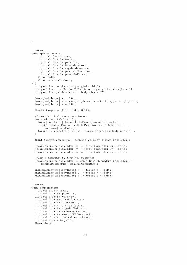
k e r n e lvoid updateMomenta (

g l o b a l f loat ∗ mass ,g l o b a l f l o a t 3 ∗ f o r c e ,g l o b a l f l o a t 3 ∗ p o s i t i o n ,g l o b a l f l o a t 3 ∗ linearMomentum ,g l o b a l f l o a t 3 ∗ angularMomentum ,g l o b a l f l o a t 3 ∗ p a r t i c l e P o s i t i o n ,g l o b a l f l o a t 3 ∗ p a r t i c l e F o r c e ,

f loat de l ta ,f loat t e r m i n a l V e l o c i t y

) {unsigned int bodyIndex = g e t g l o b a l i d (0 ) ;unsigned int tota lNumberOfPart i c l e s = g e t g l o b a l s i z e (0 ) ∗ 27 ;unsigned int p a r t i c l e I n d e x = bodyIndex ∗ 27 ;

f o r c e [ bodyIndex ] . x = 0 .0 f ;f o r c e [ bodyIndex ] . y = mass [ bodyIndex ] ∗ −9.81 f ; // f o r c e o f g r a v i t yf o r c e [ bodyIndex ] . z = 0 .0 f ;

f l o a t 3 torque = {0 .0 f , 0 . 0 f , 0 . 0 f } ;

// Ca l cu la t e body f o r c e and torquefor ( int i =0; i <27; i++) {

f o r c e [ bodyIndex ] += p a r t i c l e F o r c e [ p a r t i c l e I n d e x+i ] ;f l o a t 3 r e l a t i v e P o s = p a r t i c l e P o s i t i o n [ p a r t i c l e I n d e x+i ] −

p o s i t i o n [ bodyIndex ] ;torque += c r o s s ( r e l a t i v e P o s , p a r t i c l e F o r c e [ p a r t i c l e I n d e x+i ] ) ;

}

f loat terminalMomentum = t e r m i n a l V e l o c i t y ∗ mass [ bodyIndex ] ;

linearMomentum [ bodyIndex ] . x += f o r c e [ bodyIndex ] . x ∗ d e l t a ;linearMomentum [ bodyIndex ] . y += f o r c e [ bodyIndex ] . y ∗ d e l t a ;linearMomentum [ bodyIndex ] . z += f o r c e [ bodyIndex ] . z ∗ d e l t a ;

// Limit momentum by termina l momentumlinearMomentum [ bodyIndex ] = clamp ( linearMomentum [ bodyIndex ] , −

terminalMomentum , terminalMomentum ) ;

angularMomentum [ bodyIndex ] . x += torque . x ∗ d e l t a ;angularMomentum [ bodyIndex ] . y += torque . y ∗ d e l t a ;angularMomentum [ bodyIndex ] . z += torque . z ∗ d e l t a ;

}

k e r n e lvoid performStep (

g l o b a l f loat ∗ mass ,g l o b a l f l o a t 3 ∗ p o s i t i o n ,g l o b a l f l o a t 3 ∗ v e l o c i t y ,g l o b a l f l o a t 3 ∗ linearMomentum ,g l o b a l f l o a t 4 ∗ quaternion ,g l o b a l f loat ∗ rotat ionMatr ix ,g l o b a l f l o a t 3 ∗ angu larVe loc i ty ,g l o b a l f l o a t 3 ∗ angularMomentum ,g l o b a l f l o a t 3 ∗ i n i t i a l I I T D i a g o n a l ,g l o b a l f loat ∗ i n v e r s e I n e r t i a T e n s o r ,g l o b a l f loat ∗ bodyVBO,

f loat de l ta ,

67

f loat par t i c l eRad iu s ,int bodyVBOStride

) {unsigned int bodyIndex = g e t g l o b a l i d (0 ) ;unsigned int bodyVBOIndex = bodyIndex ∗ 24 ∗ 3 ;unsigned int matrixIndex = bodyIndex ∗ 9 ;

//Update i n v e r s e i n e r t i a tensor{

f loat a = rotat ionMatr ix [ matrixIndex ] ;f loat b = rotat ionMatr ix [ matrixIndex +1] ;f loat c = rotat ionMatr ix [ matrixIndex +2] ;f loat d = rotat ionMatr ix [ matrixIndex +3] ;f loat e = rotat ionMatr ix [ matrixIndex +4] ;f loat f = rotat ionMatr ix [ matrixIndex +5] ;f loat g = rotat ionMatr ix [ matrixIndex +6] ;f loat h = rotat ionMatr ix [ matrixIndex +7] ;f loat i = rotat ionMatr ix [ matrixIndex +8] ;

f loat u = i n i t i a l I I T D i a g o n a l [ bodyIndex ] . x ;f loat v = i n i t i a l I I T D i a g o n a l [ bodyIndex ] . y ;f loat w = i n i t i a l I I T D i a g o n a l [ bodyIndex ] . z ;

i n v e r s e I n e r t i a T e n s o r [ matrixIndex ] = u∗a∗a + b∗b∗v + c∗c∗w;i n v e r s e I n e r t i a T e n s o r [ matrixIndex +1] = a∗d∗u + b∗e∗v + c∗ f ∗w;i n v e r s e I n e r t i a T e n s o r [ matrixIndex +2] = a∗g∗u + b∗h∗v + c∗ i ∗w;i n v e r s e I n e r t i a T e n s o r [ matrixIndex +3] = a∗d∗u + b∗e∗v + c∗ f ∗w;i n v e r s e I n e r t i a T e n s o r [ matrixIndex +4] = u∗d∗d + e∗e∗v + f ∗ f ∗w;i n v e r s e I n e r t i a T e n s o r [ matrixIndex +5] = d∗g∗u + e∗h∗v + f ∗ i ∗w;i n v e r s e I n e r t i a T e n s o r [ matrixIndex +6] = a∗g∗u + b∗h∗v + c∗ i ∗w;i n v e r s e I n e r t i a T e n s o r [ matrixIndex +7] = d∗g∗u + e∗h∗v + f ∗ i ∗w;i n v e r s e I n e r t i a T e n s o r [ matrixIndex +8] = u∗g∗g + h∗h∗v + i ∗ i ∗w;

}

//Perform l i n e a r s t e p{

v e l o c i t y [ bodyIndex ] . x = linearMomentum [ bodyIndex ] . x / mass [bodyIndex ] ;

v e l o c i t y [ bodyIndex ] . y = linearMomentum [ bodyIndex ] . y / mass [bodyIndex ] ;

v e l o c i t y [ bodyIndex ] . z = linearMomentum [ bodyIndex ] . z / mass [bodyIndex ] ;

p o s i t i o n [ bodyIndex ] . x += v e l o c i t y [ bodyIndex ] . x ∗ d e l t a ;p o s i t i o n [ bodyIndex ] . y += v e l o c i t y [ bodyIndex ] . y ∗ d e l t a ;p o s i t i o n [ bodyIndex ] . z += v e l o c i t y [ bodyIndex ] . z ∗ d e l t a ;

}

//Perform angular s t e p{

//Update angular v e l o c i t y{

f loat a = i n v e r s e I n e r t i a T e n s o r [ matrixIndex ] ;f loat b = i n v e r s e I n e r t i a T e n s o r [ matrixIndex +1] ;f loat c = i n v e r s e I n e r t i a T e n s o r [ matrixIndex +2] ;f loat d = i n v e r s e I n e r t i a T e n s o r [ matrixIndex +3] ;f loat e = i n v e r s e I n e r t i a T e n s o r [ matrixIndex +4] ;f loat f = i n v e r s e I n e r t i a T e n s o r [ matrixIndex +5] ;f loat g = i n v e r s e I n e r t i a T e n s o r [ matrixIndex +6] ;f loat h = i n v e r s e I n e r t i a T e n s o r [ matrixIndex +7] ;f loat i = i n v e r s e I n e r t i a T e n s o r [ matrixIndex +8] ;

68

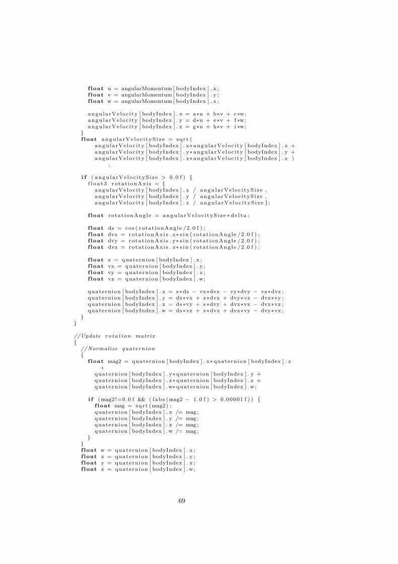
f loat u = angularMomentum [ bodyIndex ] . x ;f loat v = angularMomentum [ bodyIndex ] . y ;f loat w = angularMomentum [ bodyIndex ] . z ;

angu la rVe loc i ty [ bodyIndex ] . x = a∗u + b∗v + c∗w;angu la rVe loc i ty [ bodyIndex ] . y = d∗u + e∗v + f ∗w;angu la rVe loc i ty [ bodyIndex ] . z = g∗u + h∗v + i ∗w;

}f loat a n g u l a r V e l o c i t y S i z e = s q r t (

angu la rVe loc i ty [ bodyIndex ] . x∗ angu la rVe loc i ty [ bodyIndex ] . x +angu la rVe loc i ty [ bodyIndex ] . y∗ angu la rVe loc i ty [ bodyIndex ] . y +angu la rVe loc i ty [ bodyIndex ] . z∗ angu la rVe loc i ty [ bodyIndex ] . z )

;

i f ( a n g u l a r V e l o c i t y S i z e > 0 .0 f ) {f l o a t 3 r o t a t i o n A x i s = {

angu la rVe loc i ty [ bodyIndex ] . x / a n g u l a r V e l o c i t y S i z e ,angu la rVe loc i ty [ bodyIndex ] . y / a n g u l a r V e l o c i t y S i z e ,angu la rVe loc i ty [ bodyIndex ] . z / a n g u l a r V e l o c i t y S i z e } ;

f loat ro tat ionAng le = a n g u l a r V e l o c i t y S i z e ∗ d e l t a ;

f loat ds = cos ( ro tat ionAng le /2 .0 f ) ;f loat dvx = r o t a t i o n A x i s . x∗ s i n ( ro tat ionAng le /2 .0 f ) ;f loat dvy = r o t a t i o n A x i s . y∗ s i n ( ro tat ionAng le /2 .0 f ) ;f loat dvz = r o t a t i o n A x i s . z∗ s i n ( ro tat ionAng le /2 .0 f ) ;

f loat s = quatern ion [ bodyIndex ] . x ;f loat vx = quatern ion [ bodyIndex ] . y ;f loat vy = quatern ion [ bodyIndex ] . z ;f loat vz = quatern ion [ bodyIndex ] . w;

quatern ion [ bodyIndex ] . x = s ∗ds − vx∗dvx − vy∗dvy − vz∗dvz ;quatern ion [ bodyIndex ] . y = ds∗vx + s ∗dvx + dvy∗vz − dvz∗vy ;quatern ion [ bodyIndex ] . z = ds∗vy + s ∗dvy + dvz∗vx − dvx∗vz ;quatern ion [ bodyIndex ] . w = ds∗vz + s ∗dvz + dvx∗vy − dvy∗vx ;

}}

//Update r o t a t i o n matrix{

// Normalize quaternion{

f loat mag2 = quatern ion [ bodyIndex ] . x∗ quatern ion [ bodyIndex ] . x+

quatern ion [ bodyIndex ] . y∗ quatern ion [ bodyIndex ] . y +quatern ion [ bodyIndex ] . z∗ quatern ion [ bodyIndex ] . z +quatern ion [ bodyIndex ] . w∗ quatern ion [ bodyIndex ] . w;

i f (mag2 !=0.0 f && ( fabs (mag2 − 1 .0 f ) > 0.00001 f ) ) {f loat mag = s q r t (mag2) ;quatern ion [ bodyIndex ] . x /= mag ;quatern ion [ bodyIndex ] . y /= mag ;quatern ion [ bodyIndex ] . z /= mag ;quatern ion [ bodyIndex ] . w /= mag ;

}}f loat w = quatern ion [ bodyIndex ] . x ;f loat x = quatern ion [ bodyIndex ] . y ;f loat y = quatern ion [ bodyIndex ] . z ;f loat z = quatern ion [ bodyIndex ] . w;

69

f loat xx = x ∗ x ;f loat yy = y ∗ y ;f loat zz = z ∗ z ;f loat xy = x ∗ y ;f loat xz = x ∗ z ;f loat yz = y ∗ z ;f loat wx = w ∗ x ;f loat wy = w ∗ y ;f loat wz = w ∗ z ;

ro tat ionMatr ix [ matrixIndex ] = 1 .0 f −2.0 f ∗( yy+zz ) ;ro tat ionMatr ix [ matrixIndex +1] = 2 .0 f ∗( xy−wz) ;ro tat ionMatr ix [ matrixIndex +2] = 2 .0 f ∗( xz+wy) ;ro tat ionMatr ix [ matrixIndex +3] = 2 .0 f ∗( xy+wz) ;ro tat ionMatr ix [ matrixIndex +4] = 1 .0 f −2.0 f ∗( xx+zz ) ;ro tat ionMatr ix [ matrixIndex +5] = 2 .0 f ∗( yz−wx) ;ro tat ionMatr ix [ matrixIndex +6] = 2 .0 f ∗( xz−wy) ;ro tat ionMatr ix [ matrixIndex +7] = 2 .0 f ∗( yz+wx) ;ro tat ionMatr ix [ matrixIndex +8] = 1 .0 f −2.0 f ∗( xx+yy ) ;

}

//Update body VBO{

f loat s i d e = p a r t i c l e R a d i u s ∗ 3 .0 f ;

f loat normals [ 6 ] [ 3 ] = { // Cube face normals{ −1.0 f , 0 . 0 f , 0 . 0 f } , { 0 .0 f , 1 . 0 f , 0 . 0 f } , { 1 .0 f , 0 . 0 f ,

0 . 0 f } ,{ 0 .0 f , −1.0 f , 0 . 0 f } , { 0 .0 f , 0 . 0 f , 1 . 0 f } , { 0 .0 f , 0 . 0 f ,

−1.0 f } } ;int f a c e I n d i c e s [ 6 ] [ 4 ] = { // Cube f a c e s ’ v e r t e x i n d i c e s{ 0 , 1 , 2 , 3 } , { 3 , 2 , 6 , 7 } , { 7 , 6 , 5 , 4 } ,{ 4 , 5 , 1 , 0 } , { 5 , 6 , 2 , 1 } , { 7 , 4 , 0 , 3 } } ;

f loat v e r t i c e s [ 8 ] [ 3 ] = { // Cube v e r t e x p o s i t i o n s{ −s ide , −s ide , s i d e } , { −s ide , −s ide , −s i d e } , { −s ide ,

s ide , −s i d e } ,{ −s ide , s ide , s i d e } , { s ide , −s ide , s i d e } , { s ide , −s ide ,

−s i d e } ,{ s ide , s ide , −s i d e } , { s ide , s ide , s i d e } } ;

for ( int i =0; i <6; i++) { // f o r every facefor ( int j =0; j <4; j++) { // f o r every v e r t e x in the face

f loat r0 = rotat ionMatr ix [ matrixIndex ] ;f loat r1 = rotat ionMatr ix [ matrixIndex +1] ;f loat r2 = rotat ionMatr ix [ matrixIndex +2] ;f loat r3 = rotat ionMatr ix [ matrixIndex +3] ;f loat r4 = rotat ionMatr ix [ matrixIndex +4] ;f loat r5 = rotat ionMatr ix [ matrixIndex +5] ;f loat r6 = rotat ionMatr ix [ matrixIndex +6] ;f loat r7 = rotat ionMatr ix [ matrixIndex +7] ;f loat r8 = rotat ionMatr ix [ matrixIndex +8] ;

f loat v0 = v e r t i c e s [ f a c e I n d i c e s [ i ] [ j ] ] [ 0 ] ;f loat v1 = v e r t i c e s [ f a c e I n d i c e s [ i ] [ j ] ] [ 1 ] ;f loat v2 = v e r t i c e s [ f a c e I n d i c e s [ i ] [ j ] ] [ 2 ] ;

bodyVBO [ bodyVBOIndex ] = r0 ∗v0 + r1 ∗v1 + r2 ∗v2 + p o s i t i o n [bodyIndex ] . x ;

bodyVBO [ bodyVBOIndex+1] = r3 ∗v0 + r4 ∗v1 + r5 ∗v2 + p o s i t i o n [

70

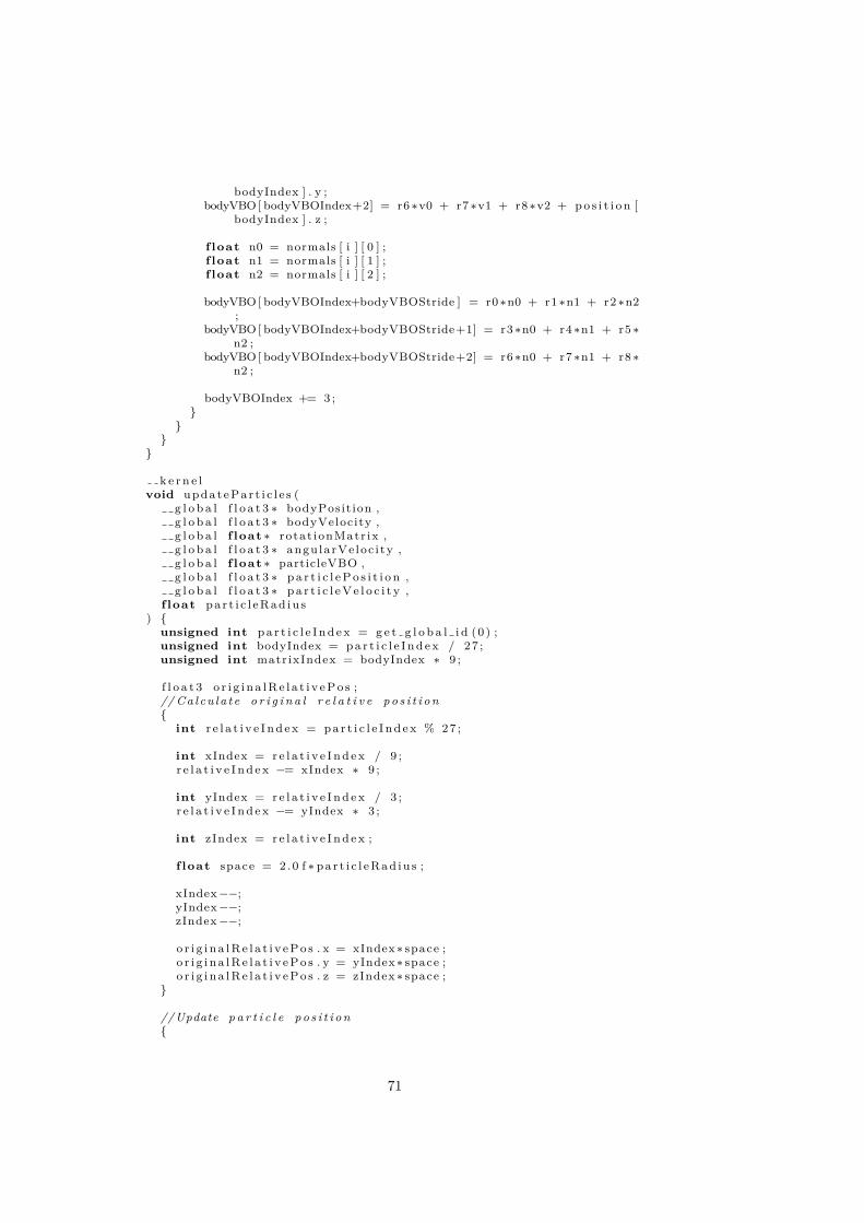
bodyIndex ] . y ;bodyVBO [ bodyVBOIndex+2] = r6 ∗v0 + r7 ∗v1 + r8 ∗v2 + p o s i t i o n [

bodyIndex ] . z ;

f loat n0 = normals [ i ] [ 0 ] ;f loat n1 = normals [ i ] [ 1 ] ;f loat n2 = normals [ i ] [ 2 ] ;

bodyVBO [ bodyVBOIndex+bodyVBOStride ] = r0 ∗n0 + r1 ∗n1 + r2 ∗n2;

bodyVBO [ bodyVBOIndex+bodyVBOStride+1] = r3 ∗n0 + r4 ∗n1 + r5 ∗n2 ;

bodyVBO [ bodyVBOIndex+bodyVBOStride+2] = r6 ∗n0 + r7 ∗n1 + r8 ∗n2 ;

bodyVBOIndex += 3 ;}

}}

}

k e r n e lvoid u p d a t e P a r t i c l e s (

g l o b a l f l o a t 3 ∗ bodyPosit ion ,g l o b a l f l o a t 3 ∗ bodyVelocity ,g l o b a l f loat ∗ rotat ionMatr ix ,g l o b a l f l o a t 3 ∗ angu larVe loc i ty ,g l o b a l f loat ∗ particleVBO ,g l o b a l f l o a t 3 ∗ p a r t i c l e P o s i t i o n ,g l o b a l f l o a t 3 ∗ p a r t i c l e V e l o c i t y ,

f loat p a r t i c l e R a d i u s) {

unsigned int p a r t i c l e I n d e x = g e t g l o b a l i d (0 ) ;unsigned int bodyIndex = p a r t i c l e I n d e x / 27 ;unsigned int matrixIndex = bodyIndex ∗ 9 ;

f l o a t 3 o r i g i n a l R e l a t i v e P o s ;// Ca l cu la t e o r i g i n a l r e l a t i v e p o s i t i o n{

int r e l a t i v e I n d e x = p a r t i c l e I n d e x % 27 ;

int xIndex = r e l a t i v e I n d e x / 9 ;r e l a t i v e I n d e x −= xIndex ∗ 9 ;

int yIndex = r e l a t i v e I n d e x / 3 ;r e l a t i v e I n d e x −= yIndex ∗ 3 ;

int zIndex = r e l a t i v e I n d e x ;

f loat space = 2 .0 f ∗ p a r t i c l e R a d i u s ;

xIndex−−;yIndex−−;zIndex−−;

o r i g i n a l R e l a t i v e P o s . x = xIndex∗ space ;o r i g i n a l R e l a t i v e P o s . y = yIndex∗ space ;o r i g i n a l R e l a t i v e P o s . z = zIndex ∗ space ;

}

//Update p a r t i c l e p o s i t i o n{

71

p a r t i c l e P o s i t i o n [ p a r t i c l e I n d e x ] . x =o r i g i n a l R e l a t i v e P o s . x∗ ro tat ionMatr ix [ matrixIndex ] +o r i g i n a l R e l a t i v e P o s . y∗ ro tat ionMatr ix [ matrixIndex +1] +o r i g i n a l R e l a t i v e P o s . z∗ ro tat ionMatr ix [ matrixIndex +2] ;

p a r t i c l e P o s i t i o n [ p a r t i c l e I n d e x ] . y =o r i g i n a l R e l a t i v e P o s . x∗ ro tat ionMatr ix [ matrixIndex +3] +o r i g i n a l R e l a t i v e P o s . y∗ ro tat ionMatr ix [ matrixIndex +4] +o r i g i n a l R e l a t i v e P o s . z∗ ro tat ionMatr ix [ matrixIndex +5] ;

p a r t i c l e P o s i t i o n [ p a r t i c l e I n d e x ] . z =o r i g i n a l R e l a t i v e P o s . x∗ ro tat ionMatr ix [ matrixIndex +6] +o r i g i n a l R e l a t i v e P o s . y∗ ro tat ionMatr ix [ matrixIndex +7] +o r i g i n a l R e l a t i v e P o s . z∗ ro tat ionMatr ix [ matrixIndex +8] ;

p a r t i c l e P o s i t i o n [ p a r t i c l e I n d e x ] . x += bodyPos i t ion [ bodyIndex ] . x ;p a r t i c l e P o s i t i o n [ p a r t i c l e I n d e x ] . y += bodyPos i t ion [ bodyIndex ] . y ;p a r t i c l e P o s i t i o n [ p a r t i c l e I n d e x ] . z += bodyPos it ion [ bodyIndex ] . z ;

}

//Update p a r t i c l e v e l o c i t yf loat s c a l a r = s q r t (

ang u la rVe loc i ty [ bodyIndex ] . x∗ ang u la rVe loc i ty [ bodyIndex ] . x +ang u la rVe loc i ty [ bodyIndex ] . y∗ angu la rVe loc i ty [ bodyIndex ] . y +ang u la rVe loc i ty [ bodyIndex ] . z∗ angu la rVe loc i ty [ bodyIndex ] . z ) ;

s c a l a r ∗= s c a l a r ;

p a r t i c l e V e l o c i t y [ p a r t i c l e I n d e x ] . x = bodyVeloc ity [ bodyIndex ] . x ;p a r t i c l e V e l o c i t y [ p a r t i c l e I n d e x ] . y = bodyVeloc ity [ bodyIndex ] . y ;p a r t i c l e V e l o c i t y [ p a r t i c l e I n d e x ] . z = bodyVeloc ity [ bodyIndex ] . z ;

i f ( s c a l a r > 0 .0 f ) {f l o a t 3 r e l a t i v e P o s i t i o n = {

p a r t i c l e P o s i t i o n [ p a r t i c l e I n d e x ] . x−bodyPos i t ion [ bodyIndex ] . x ,p a r t i c l e P o s i t i o n [ p a r t i c l e I n d e x ] . y−bodyPos i t ion [ bodyIndex ] . y ,p a r t i c l e P o s i t i o n [ p a r t i c l e I n d e x ] . z−bodyPos i t ion [ bodyIndex ] . z

} ;

f loat s c a l a r 2 = (ang u la rVe loc i ty [ bodyIndex ] . x∗ r e l a t i v e P o s i t i o n . x +ang u la rVe loc i ty [ bodyIndex ] . y∗ r e l a t i v e P o s i t i o n . y +ang u la rVe loc i ty [ bodyIndex ] . z∗ r e l a t i v e P o s i t i o n . z) / s c a l a r ;

f l o a t 3 term = {r e l a t i v e P o s i t i o n . x − angu la rVe loc i ty [ bodyIndex ] . x∗ s c a l a r2 ,r e l a t i v e P o s i t i o n . y − angu la rVe loc i ty [ bodyIndex ] . y∗ s c a l a r2 ,r e l a t i v e P o s i t i o n . z − angu la rVe loc i ty [ bodyIndex ] . z∗ s c a l a r 2 } ;

p a r t i c l e V e l o c i t y [ p a r t i c l e I n d e x ] . x += ( an gu la rV e loc i ty [ bodyIndex] . y∗ term . z − ang u la rVe loc i ty [ bodyIndex ] . z∗ term . y ) ;

p a r t i c l e V e l o c i t y [ p a r t i c l e I n d e x ] . y += ( an gu la rV e loc i ty [ bodyIndex] . z∗ term . x − ang u la rVe loc i ty [ bodyIndex ] . x∗ term . z ) ;

p a r t i c l e V e l o c i t y [ p a r t i c l e I n d e x ] . z += ( angu l a rVe l oc i ty [ bodyIndex] . x∗ term . y − ang u la rVe loc i ty [ bodyIndex ] . y∗ term . x ) ;

}

//Update p a r t i c l e VBOunsigned int particleVBOIndex = p a r t i c l e I n d e x ∗ 3 ;

72

particleVBO [ particleVBOIndex ] = p a r t i c l e P o s i t i o n [ p a r t i c l e I n d e x ] . x;

particleVBO [ particleVBOIndex +1] = p a r t i c l e P o s i t i o n [ p a r t i c l e I n d e x] . y ;

particleVBO [ particleVBOIndex +2] = p a r t i c l e P o s i t i o n [ p a r t i c l e I n d e x] . z ;

}

73