Real-Time Queueing Theory - ann.ece.ufl.edu · to queueing models greatly complicates the analysis of ... (‘heavy traffic” case ... real-time queueing theory that is being presented

Real-Time Queueing Theory

John P. Lehoczky Department of Statistics

Carnegie Mellon University Pittsburgh, PA 15213

Abstract

This paper presents a new approach to real-time system scheduling. The approach, called real-time queueing theory, includes customer timing requirements into queueing models. With real-time queueing models, one is able to explicitly characterize the dynamic behavior of the customer lead-tame profile process where lead-time = deadline minus current time. In spite of the injinite dimensionality of these processes, in the heavy trafic case, a simple description of lead-time profile process is presented, and this description is shown to be very accurate when compared against simulations. Real-tame queueing theory offers the promise of providing real-time system predictabil- ity for systems characterized b y substantial stochastic behavior (such as ATM networks and multimedia systems). Possible generalizations are discussed.l

1 Introduction Real-time computer systems refer to computer and

communication systems in which the applications or tasks using the system have explicit timing requirements. The conditions for the correct performance of a real-time system include both the logical correctness of each of the tasks that are executed and also their timing correctness, that is the system should meet the timing requirements of each task. Over the last decade there has been a major effort to develop a theory of

'Research supported in part by contracts N00014-92-5-1524 and N00014-92-5-1771 from the Office of Naval Research and the DARTS Project with Lockheed Martin and Wright Laboratory.

2The real-time queueing theory research project is a joint project being carried out in collaboration with Steven Shreve and Bogdan Doytchinov of the Carnegie Mellon University De- partment of Mathematics. A paper giving the mathematical developments outlined in this paper will appear elsewhere. Some initial related ideas were discussed with and developed by Frank Kelly of University of Cambridge and David Aldous of Uni- versity of California, Berkeley. My thanks to Andrew Ng of Carnegie Mellon University who developed the simulation pro- gram from which the figures in the paper were produced and who has also contributed to some of the understandings discussed in this paper.

1052-8725196 $5.00 0 1996 IEEE

hard real-time systems, a theory which would allow, for a given task or application set, the determination of whether the timing requirements of those tasks could be met. For a theory of real-time systems to be useful in practice, it must take into account a host of important system considerations, for example operating system and scheduling overhead, hardware architec- ture, concurrency control and other sorts of blocking and task precedence relations.

Two principle approaches have been developed for assessing the design of real-time systems with periodic task arrivals, one based on a fixed task priority structure (exemplified by generalized rate monotonic scheduling) and the other based on dynamic priorities (exemplified by the earliest deadline first approach to scheduling). Both approaches have been in rapid development, and a number of actual real-time systems now use one of these two approaches. The literature related to this problem is extensive and is not reviewed here as it is no doubt well known to the reader.

In spite of these important developments in real- time scheduling, there are still major shortcomings. The most important shortcoming is that the hard real- time scheduling problem has been formulated to require a non-stochastic solution. That is, the notion of predictable system behavior has been defined to require that all tasks in the task set must meet their timing requirements with certainty. This requirement has resulted in the scheduling problem being addressed under extremely narrow assumptions, assumptions which essentially foreclose tasks with substantial variability in their execution times, dynamic task sets or dynamic environments. Tasks are assumed to require a deterministic processing time, their worst case execution time. Tasks are assumed to be periodic, or sporadic with a worst case arrival period. There has been substantial recent work on systems which consist of mixtures of periodic and aperiodic tasks; however, the aperiodic tasks are either highly constrained or their timing requirements are assumed to be soft. Further- more, the algorithms are not especially useful when

186

Authorized licensed use limited to: University of Florida. Downloaded on January 20, 2010 at 18:46 from IEEE Xplore. Restrictions apply.

the total workload is dominated by aperiodic activity. The very narrowly defined scheduling problem per-

mits the development of scheduling algorithms both with good performance and for which an explicit determination of task timing requirement feasibility can be made under fairly broad but deterministic conditions (for example the conditions supported by generalized rate monotonic scheduling). Unfortunately, this formulation is so narrow that many of the most important real-time system applications, especially those involving multimedia, real-time communications on ATM networks and robotics problems, cannot be addressed. Those applications have task processing times which are stochastic, especially in the multimedia context where voice and video transmissions exhibit great variability and may involve dynamic environments. It is simply impractical to assume a worst case execution times for each task when the execution time variance is high, because on average the system will be highly underutilized.

For real-time systems for which the task sets exhibit substantial variability, one would like to develop approaches based on queueing theory, a theory which was designed to model and predict stochastic system behavior with resource contention. This theory is based on allowing randomness in the task arrivals and task execution times. The difficulty with queueing theory is that this theory does not typically allow for explicit consideration of task timing requirements. Instead, it only permits priorities which allow important tasks or tasks with short timing requirements to receive pref- erential treatment. However, queueing theory usually focuses on general system performance measures, such as task delay, queue lengths, processor utilization, etc., and these are usually computed under equilibrium assumptions. It does not model the timing requirements of each customer, nor does it analyze the ability of a scheduling algorithm to meet those timing requirements, although this is what is needed for real-time systems. What is needed is a new theory which com- bines the focus on meeting task timing requirements as studied in real-time scheduling theory with the focus on stochastic task sets as studied in queueing theory.

The purpose of this paper is to present an introduction to a promising new theory that appears to be able to combine the best of both of these disciplines, real-time queueing theory. This theory begins from the point of view of queueing theory; however, it must be able to answer questions that arise with real- time systems, especially whether or not a system will be able to satisfy the timing requirements of a task set. Of course, adding customer timing requirements

to queueing models greatly complicates the analysis of those models. Customers will arrive with a given timing requirement, for example a particular hard deadline, i.e. an initial laxity. As time evolves, the laxity will change, depending upon which customers are receiving service and their service requirements. Thus, the state of the real-time queueing system includes not only the number of customers in the system, but also their residual service requirements and the time remaining until the deadline elapses, both of which change dynamically. Consequently, the state variable of such a queueing system is of unbounded dimension, a fact which appears to make an exact analysis extremely complex, possibly infeasible.

Fortunately, there is an approach to handling the infinite dimensional problem. For the situation in which one has a simple Markov model with Poisson arrivals and exponential service times (and arbitrary customer deadline distributions), the problem can be formulated and solved, at least in principle, although the solution is very complicated. It turns out, however, that if one focuses on the (‘heavy traffic” case (where the traffic intensity on the processor converges to l), then this very complex system has a solution characterized by a surprising simplicity. Furthermore, simulations validate these results. In addition, if one can characterize the behavior of the system under heavy traffic, one can generate a worst case bound on system performance for the smaller traffic intensities.

The reader will immediately be concerned that the real-time queueing theory that is being presented in this paper will only work for very simple queueing systems, those characterized by Poisson arrivals and exponential service times. In fact, in the heavy traffic case, the results generalize to much more general models, models with arbitrary renewal arrival processes and arbitrary service time distributions. More impor- tantly, the methodology can be extended to queueing networks, so for the first time, we have the potential to study analytically end-to-end delay and satisfaction of customer timing requirements under stochastic conditions. Finally, the methodology opens up the possibility of directly modelling, analyzing and optimizing queueing control policies, or real-time scheduling policies. It also appears that the methodology will be able to handle periodic task sets (which are tasks with degenerate renewal process arrivals) and mixtures of periodic and aperiodic tasks. In the next section we will outline the basic theory. The methods rely on a mathematically sophisticated part of the theory of stochastic processes including: weak convergence of queueing processes to reflected Brownian motion, Markov pro-

187


cesses evolving on the space of Fourier transforms and semi-group theory. In spite of this, a reader who is familiar only with the basic theory of Markov chains and queueing theory should be able to follow the present at ion.

2 The Basic Model

We introduce the ideas associated with real-time queueing theory through a simple M/M/ 1 queueing model. We make the following assumptions: A l :

A2 :

A3 :

A4:

A5 :

There is a single processor that services tasks (customers) at rate 1. Customers arrive according to a Poisson process with rate A. Customers have service requirements which require an exponential time for the server to complete with mean = l /p. Each customer arrives with a hard relative deadline drawn from a probability distribution having cumulative distribution function G, and characteristic function F(s) = s-", ei""d(z). The absolute customer deadline is the relative deadline plus the current (arrival) time. There is a queue discipline which governs the order in which customers are processed. Preemp- tion is permitted (we assume preempt-resume), and it is assumed to result in no overhead.

Assumption A5 is vague concerning the specific queue discipline or scheduling algorithm being used. In this paper, we will focus on specifically on (1) earliest deadline first (edf) and (2) processor sharing (ps). Of these two, only edf would be considered to be a real- time system scheduling algorithm. The methodology introduced here will allow for consideration of other disciplines including certain fixed priority queue disciplines, the shortest remaining processing time discipline as well as FIFO. In the analysis, the queue discipline will be represented abstractly as an operator on Fourier transforms, so that one is ultimately able to optimize system behavior with respect to the scheduling algorithm or queue discipline.

In the ordinary M/M/1 queue, there is a scalar state variable, X t , the number of customers in the system at time t . In real-time queueing theory, we want to keep much more detailed information about each of the customers. For the simple model at hand, it is sufficient to associate a dynamic variable with each customer, its lead-tzme. At time t , the lead-time of a customer is the difference between its absolute deadline and the current time, hence a customer's lead- time decreases linearly with time. During an interval

[t, t + 51, if a customer has not departed, then its lead- time is reduced by S. Negative lead-times are possible and indicate that a customer is late. In some systems with hard deadlines, lateness is not permitted. Thus when a customer becomes late, its processing is stopped and it is removed from the system with a timing fault being recorded. The theory we are de- veloping accommodate both cases in a single analysis, but we do not pursue this here.

We take as our state variable the vector S = (m, L1, . . . , Lm), where m denotes the number of customers in the system and Li denotes the lead-time of the ith customer. If the system is empty, then the state variable is the null vector, (D. There is an issue of how to order the customers, i.e. determining which customer is the ith. Of course, this will depend upon the queue discipline. For edf, it is convenient to order the customers according to increasing lead-times, i.e. so that Li 5 Lt+l. For FIFO, the lead-times are in arrival order. For processor sharing, the queue order does not matter, as all customers are being served si- multaneously with each receiving service rate l /m. It is most convenient to keep customers in arrival order.

We want to characterize the lead-time process, {&,t 2 0). This is a very high dimensional process, but we can reformulate it to obtain a simpler characterization. At any moment in time, there are n customers and each customer has an associated lead- time. Thus, at any instant, the set of lead-times can be associated with a set of unit masses on points on the real line, R1 = (-00,co). This can, in turn, be considered to be a measure on the Borel subsets of R1, where the measure of any Borel set, B , is simply the number of customers with lead-times in B. As time changes, this measure will change (1) because all lead- times of remaining customers decrease, (2) new customers arrive or (3) customers complete service and depart. Given the Markovian structure of our system, it is very easy to write the transition structure of the lead-time process. In particular, for edf, if the state at time t is given by (m, 11,. . . , lm) with m 2 1, then the state at time t + h for small h will be given by the tables below. For the processor sharing case, we keep the tasks in arrival order. In Tables 1 and 2, we assume the state at time t is (m, /I,. . . , Im). For the edf queue discipline, we keep the tasks in lead-time order with the first lead-time being the smallest. In Table 2, for simplicity only one entry is given for an arriving customer. In reality, there are m + 1 distinct entries depending upon where in the queue the arriving customer is inserted. As written, the arriving customer has the shortest lead time. As was mentioned

188


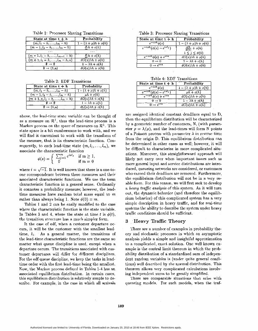
Table 1: Processor Sharing Transitions State at time t + h Probability

. (m,l1 -h,...,Im - h ) l-(A+Lb)h+o(h) (m - 1,/2 - h , . . . ,1, - h) S h + o(h)

I

( m - 1,ll - h )..., 1,-1 - h) (m + 1,11 - h, . . . ,1, - h, a)

0 + 0 91 + (la)

I ... I ... I

k h + o(h ) dG(a)Ah + o(h )

dG(a)Ah + o(h ) 1 - Ah + o(h )

. e-zsh+(s) + e t s a

0 4 0 0 + elsa

Table 2: EDF Transitions 1 State at t i m e t + h I Probabilitv I

dG(a)Ah + o(h )

dG(a)Xh + o(h ) 1 - Ah + o(h)

above, the lead-time state variable can be thought of as a measure on R1, thus the lead-time process is a Markov process on the space of measures on R1. This state space is a bit cumbersome to work with, and we will find it convenient to work with the transform of the measure, that is its characteristic function. Con- sequently, to each lead-time state (m, II, . . . , Im), we associate the characteristic function

i f m z 1, i f m = O

where i = a. It is well known that there is a one-to- one correspondence between these measures and their associated characteristic functions. We use the term characteristic function in a general sense. Ordinarily it connotes a probability measure; however, the lead- time measures have random total mass equal to m rather than always being 1. Note $(O) = m.

Tables 1 and 2 can be easily modified to the case where the characteristic function is the state variable. In Tables 3 and 4, where the state at time t is d ( t ) , the transition structure has a much simpler form.

It the case of edf, when a customer departure occurs, it will be the customer with the smallest lead- time, 11. As a general matter, the transitions of the lead-time characteristic functions are the same no matter what queue discipline is used, except when a departure occurs. The transitions associated with customer departures will differ for different disciplines. For the edf queue discipline, we keep the tasks in lead- time order with the first lead-time being the smallest. Now, the Markov process defined in Tables 1-4 has an associated equilibrium distribution. In certain cases, this equilibrium distribution is relatively simple to describe. For example, in the case in which all arrivals

Table 3: Processor Sharing Transitions 1 State at t i m e t + h I Probabilitv 1

Table 4: EDF Transitions

I , \ ,

0 + etsa I dG(a)Ah + o(h)

are assigned identical constant deadlines equal to D, then the equilibrium distribution will be characterized by a geometric number of customers, N, (with parameter p = X / p ) , and the lead-times will form N points of a Poisson process with parameter X in reverse time from the origin D. This equilibrium distribution can be determined in other cases as well; however, it will be difficult to characterize in more complicated situations. Moreover, this straightforward approach will likely not carry over when important issues such as more general input and service distributions are introduced, queueing networks are considered, or customers who exceed their deadlines are removed. Furthermore, the equilibrium distribution will not be in a very us- able form. For this reason, we will first seek to develop a heavy trafic analysis of this system. As it will turn out, the dynamic behavior (and therefore the equilibrium behavior) of this complicated system has a very simple description in heavy traffic, and for real-time systems the ability to describe the system under heavy traffic conditions should be sufficient.

3 Heavy Traffic Theory There are a number of examples in probability the-

ory and stochastic processes in which an asymptotic analysis yields a simple and insightful approximation to a complicated, exact solution. One well known example is the central limit theorem in which the probability distribution of a standardized sum of independent random variables is (under quite general conditions) well described by the normal distribution. This theorem allows very complicated calculations involving independent sums to be greatly simplified.

There are comparable situations that arise with queueing models. For such models, when the traf-

189


fic intensity is relatively large, the queueing model has substantial fluctuations. By properly rescaling both time and space, it is possible to approximate the discrete queueing system by a continuous diffusion process, usually a Brownian motion process with a reflecting barrier at the origin. Just as calculations involving sums of independent random variables can be reduced to simpler calculation involving the normal distribution, the dynamic behavior of queueing systems can (in heavy traffic) be expressed in terms of the behavior of a Brownian motion, a continuous time, continuous state diffusion process about which much is known. Also, the weak convergence of queueing systems to Brownian motion is a rather general result which applies when the arrival process is a renewal process (rather than requiring Poisson process arrivals) and service times are general (rather than requiring exponential service). Moreover, there has been a great deal of recent research extending the single queueing system results to queueing networks. In particular, it is now possible to model general Jackson queueing networks as Brownzan networks, the higher dimensional analog of Brownian motion. Finally, there is a fairly well-developed theory of optimal control of Brownian motion. This means that if one can approximate a queueing system as a Brownian network, then one can also develop the optimal control (in the sense of customer scheduling, input control and network flow control) of such systems.

The development of the theory of Brownian networks is rather deep mathematically; however, the interested reader should begin by consulting the excellent work by Harrison[S, 4, 51. An interesting recent paper by Dai[2] also contains a large number of relevant references. The reader should also consult the seminal 1979 Ph.D. dissertation of Burman[l] which provides a methodology for handling the boundary problems that arise when proving that queueing systems converge to limiting diffusion processes. Burman also develops the method of perturbed test functions to extend the weak convergence results to queues with renewal process arrivals and general service times. Thus, there is a substantial amount of mathematical machinery available to extend the basic model presented in this paper to general queueing networks.

The scaling of time and space that results in the weak convergence of a sequence of queueing systems to a limiting diffusion process is similar to the scaling used for the central limit theorem which applies to the sum of n random variables, each of which has been scaled by fi. A queueing system evolves over

There is a large literature on these topics.

time. If the arrival and service rates are both 0(1), then during any time interval of length t , there will be 0(1) transitions. If we want the number of transitions to be large, then we must "speed up" time. If we want there to be O(n) transitions (which would be appropriate for the central limit theorem to apply), then we must speed up time by a factor of n. In addition, we need to scale the size of each of these changes by 1/+. Consequently, if Q(t ) represents the queue length at time t , we want to consider the scaled ver- sion of this process, X(.)(t) = & ( n t ) / f i . Now, for this scaled process to converge to a non-degenerate limit, it is necessary to have the traffic intensity nearly equal to 1. Thus, we introduce the heavy trafic con- dition, the arrival rate A, = X ( l - y/+) and the service rate p, = X. Thus, the traffic intensity parameter is given by p. = l - y/fi. It is well-known (see for example Burman[l]) that the sequence of processes { X ( " ) ( t ) , t > 0) converges weakly to a reflected Brownian motion with drift -y and scale 2X.

This methodology can be extended in a straightforward way to more general queueing systems. For example, if one assumes a GI/M/1 model, then one needs to supplement the state space with a second variable giving the time since the last arrival. Using the method of perturbed test functions (see Burman[l]), one can determine the limiting queueing process for this model. Burman also handles non-exponential service times and studies Jackson networks.

The Brownian network methodology has been suc- cessfully applied to queueing networks that arise in manufacturing problems, especially the reentrant work-flow structure of VLSI semiconductor fabrica- tion. Harrison and Wein[6] and Wein[7] present the initial development of the Brownian network model for such applications and work out the optimal scheduling policies in the sense of task sequencing at a station and input control. Although the theory relies on heavy traffic, it turns out that it offers accurate prediction for realistic systems, so there is good reason to believe that real-time queueing theory will offer accurate predictions for real-time systems of interest.

In Section 4, we apply the methodology to the Markov processes defined in Tables 1-4 having an infinite dimensional state space defined by the number of customers in the queue and the dynamically chang- ing lead-times of each. The scaled lead-time process will, in heavy traffic, converge to a recognizable limit which we can use to analyze the performance of the real-time queueing system in terms of customer deadline performance.

190


4 Heavy Traffic Analysis of Customer Lead-Times

The real-time queues studied in this paper are formulated as Markov processes with characteristic functions as the state variable. The first step in analyzing such processes is to determine the infinitesimal generator of the Markov process. To do this, we introduce a Banach space, a, of complex valued functions which contain the characteristic functions, and we re- gard {+(s ; t ) , t > 0) as a Markov process with state space a. To calculate the infinitesimal generator, we introduce a collection of smooth mappings H from @ to E. By smooth, we mean that H must be at least twice Frechet differentiable. The infinitesimal generator is then defined by an operator A with domain given by a collection of smooth functionals on @ for which the limit below exists:

We begin by presenting a simple calculation for the one dimensional case, the infinitesimal generator for the scaled queue length process in a simple M/M/l queue and then show how, under heavy traffic, it converges to a Brownian motion process. The reader is referred to Burman[l] for this example and the mathematical analysis proving weak convergence.

Suppose Q(t ) represents the number in the M/M/l system at time t and let X ( " ) ( t ) = Q ( n t ) / f i be the scaled queue length process at time t. There are two possible transitions that can occur: (1) an arrival which adds l / f i to the X ( " ) process and (2) a service completion (provided the queue is not empty) which reduces the X ( " ) process by l/fi. Recall that we are assuming heavy traffic conditions, A(") = A( 1 - y/f i) and ,U(") = A. The infinitesimal generator is given by an operator A on functions f defined by the following for x 2 I/+:

A(f) = A ( 1 - ~ / 6 ) 4 f ( ~ + 1 / 6 1 - f(x)) +Xn(f(. - V f i ) - f(.)). (2)

We next expand in a Taylor series in powers of n and collect terms. The equation must be slightly modified when 0 5 2 < $=, because there are no customers in the queue to service. In order for a limit t o exist as n + 00, we must put the restriction f'(0) = 0 onto the function f. This gives, for functions f satisfying f'(0) = 0,

d(f) = -yf'(e) + A.f"(x>. (3)

The above infinitesimal generator can be recognized as the generator corresponding to a Brownian motion with drift -7 and scale 2X and a reflecting barrier at the origin. In real-time queueing theory, we will also need to scale customer deadlines by fi, since the mean number in the queue is p ( " ) / ( l - p ( " ) ) = O(fi).

We now apply the same method to the lead-time process as defined in Tables 3 and 4. We must scale the lead-time process appropriately (so that it converges to a limit under heavy traffic) and work out its associated infinitesimal generator. Under the heavy traffic assumption, the queue length and customer delay will be O(fi). Thus, we must assume that deadlines are a comparable order of magnitude, O(fi), and lead-times will also be of the same order of magnitude. Specifically, deadlines, D("), will have characteristic function r(")(s) = I'(fis), where r(s) is the characteristic function corresponding to G. Thus, if &(t) represents the lead-time of the j th customer in the queue at time t , then we should, under heavy traffic, consider instead Lj ( n t ) / f i and the scaled characteristic function of the lead-times,

To calculate the generator of the {+(")(s; t ) , t 2 0) process, we refer to the transition structure defined in Tables 3 and 4. There are three transition types to calculate: aging, arrival and service.

The aging term is the simplest. During an interval of length [t, t+h], with probability 1 - (A(") + , ~ ( " ) ) n h + o(h), neither an arrival nor a departure occurs; however, during this time period, the lead-time of each customers in queue will decrease by nh. This will contribute a term to the generator of the form:

+'" ' (s; t ) = (C3=l Q(n') easL>(nt)/fi)/fi.

.(1 - (A(") + p("))nh + o(h)) /h . (4)

Assuming H is Frechet differentiable, taking the limit produces the term

V f i H ( + ( " ) ( s ) ) ( -is+(") (s)), (5)

where V H denotes the first Frechet derivative of H . The arrival term can be calculated in a similar fash-

ion. The transition probability associated with arrivals is A(")nh + o(h). Since this is already O(h), we can ignore the changes in customer lead-times over this interval and just capture the arrival. The contribution to the infinitesimal generator is the term

191


This term cannot be reduced, except we can expand the H difference into powers of 6. The highest order term in the integrand becomes A(")fiVH(d(")(s)) s-", e i " f idG(a) . Recognizing the integral, we find the highest order term to be

&V H (d(")( s ) ) (A( " ) r ( s ) ) . (7)

There are other lower order terms that must be considered; however, in this paper we just present the highest order terms.

The third term corresponds to customer departures from service completions, and its specific form will depend on the queue discipline. We first consider processor sharing. During [t,t+h], there is a probability p(")nh/+(")(O)+o(h) that customer j , 1 5 j 5 +(")(O), will depart (assuming the queue is non-empty). The contribution of these transitions to the generator is

(8) Again assuming H is smooth and expanding in a power series in powers of n-b and computing the sum, the highest order term is given by

f i V H ( + ( " ) ( s)( -p'"')+'"'(s)/+'"'( 0 ) ) . (9)

Now we combine the three O(& terms given by equations (5), (7) and (9) to obtain the highest order term of the limiting infinitesimal generator for the lead-time characteristic function process. The highest order term is given by:

(10) Under heavy traffic, p(") = X and A(") = X(l-y/fi). When these assumptions are invoked in the above equation, we still have an O(&) term, plus many O( 1) terms which are not displayed. Since the Markov process governing the lead-time process must have an equilibrium distribution, this fi term must be 0(1). Consequently, d(") (~ ) must converge to a limiting characteristic function, d(s), which satisfies:

o = -is+(s) - x+(~)/+(o) + )cr(s). (11)

The above equation defines the limiting characteristic function, +(s) , up to one parameter, +(O), the number in the queue. Thus, once the number in the queue is known, the first order term characterizing the characteristic function of the lead-time distribution can be determined by (1 1).

It is straightforward to solve equation ( l l ) , namely

d(s) = W s ) / ( ( V + ( O ) > + is). (12)

This characteristic function is easily interpreted as it corresponds to the convolution of two distributions, the deadline distribution of the arriving customers, and the negative of an exponential distribution (that is, an exponential distribution on (-m,O]) with parameter X/+(O) and total mass +(O), the length of the queue at that instant. Thus, if one knows the current length of the queue, d(O), then (12) gives the Fourier transform of the instantaneous customer lead- time profile. That is, to first order, we characterize the lead-time profile process as having two components: (1) a queue length which is described as a Brownian motion with drift -7, scale 2X and a reflecting barrier at 0 and (2) given the queue length a lead-time profile given by (12). Thus the lead-time profile process is, to first order, a Brownian motion on a manifold of characteristic functions given by (12).

Next consider the edf case. The aging term given in (5) and the arrival term given in (7) will be the same; however, the departure term given by (8) and (9) must be altered. Under edf, the customer that departs is always the customer with the smallest lead- time, L1. Thus, the contribution to the generator is given by

(H(+(")(s) - eis*l /fi) - H(+(")(s)))p(")n. (13)

Again, assuming H is smoyth and expanding in a power series in powers of n-7, the highest order term is given by

~VH(~(") (s ) ) ( -p(n)eas ' l / f i ) . (14)

Combining (5), (7) and (14), in analogy with (11), we find for edf with G(L) = 0:

o = -isd(s) - XeisL + q s ) , (15)

where L is the left-most support point of the distribution corresponding to +(s). Equation (15) must be adjusted when G(L) > 0.

Finding the distribution corresponding to +(s) defined by (15) for any L is straightforward, and it, too, will depend upon the current queue length. Suppose the current queue length is Q. For the given queue length, Q, find the unique value, L , satisfying the equation

Q = X L m ( l - G(z))dz. (16)

This value L will be the left-most support point referred to in (15). The lead-time profile can now be

192


expressed as a probability distribution with density function given by

f(.) = X(l - G(.))/Q, L 5 2 < 00. (17)

It is important to recognize that equations (11) and (15) only describe the first order term of the heavy traffic approximation given the current queue length. This is a deterministic approximation, like an expected value for ordinary random variables. The random fluctuations in the lead-time profile are described by the lower order terms, and refined approx- imations can be developed from them. Nevertheless, we will see in the next section that this approximation, by itself, is surprisingly accurate. The most surprising finding is that once the queue length, Q, is known, the lead-time distribution can be determined very ac- curately using (11) or (15). Since the dynamic behavior of the queue length process is a reflected Brownian motion process, we have obtained a first order characterization of the customer lead-time profile process. It is one-dimensional, depending on Q alone.

5 Simulation Results

In this section, we present some representative simulation results. Recall that at any instant in time, the state of the real-time queueing system is characterized by the number of customers in the queue and a vector of lead-times associated with each customer. The results of the last section indicate that for a given queue length, the profile of customer lead-times should exhibit a particular form given by equations (12) for ps or (17) for edf. If we took an instantaneous snapshot of the lead-times, then we could plot that vector in the form of an empirical cumulative distribution function. This empirical distribution function could then be compared with the predicted lead-time profile. As time advances, this empirical distribution will change as old customers depart, new customers arrive and current customers age.

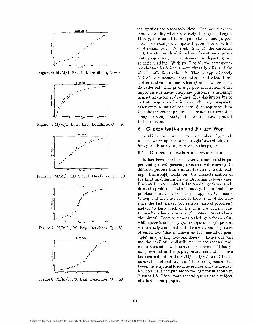
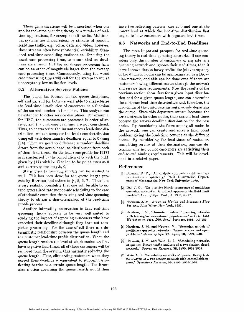
The simulations presented in Figures 1-8 are from an M/M/l queue with X = .95, p = 1.0 (hence p = .95), a deadline distribution which is either Expo- nential with mean 50 or Uniform on (0,100), a queue length of 30 or 50 and either edf or ps queue disciplines. In this heavy traffic case, the mean queue length is p/(l - p) , P(Q 2 30) = .215 and P(Q 2 50) = .077, so long queue lengths are common.

There are two clocks used in the simulation: (1) a global clock which constantly advances and (2) a local time clock which advances only when the queue length is equal to some pre-specified value (30 in Figures 1-4 and 50 in Figures 5-8). In Figures 1-4, a snapshot is

19347.9729

Figure 1: M/M/l, EDF, Exp. Deadlines, 154137415

Q = 30

Figure 2: M/M/l, EDF, Unif. Deadlines, Q = 30

taken when the local time clock reaches 500, while in Figures 5-8, a snapshot is taken when the local time clock reaches 100. Each Figure correspond to a different simulation run. The snapshot (a vector of length 30 or 50) is plotted in the form of an empirical c.d.f. and can be compared with the theoretical profile de- rived from (12) or (17). The global time when the snapshot is taken is printed on the top of each figure.

There are several observations to be made from Fig- ures 1-8. First, comparing 1 with 2, 3 with 4 etc., one can observe the impact of the deadline distribution on the lead-time profiles, that is the change in shape in the lead-time profiles. Second, note the surprising agreement between the empirical lead-time profiles and the first-order approximationsfor Q = 50 (Figures 5-8). This is quite promising, because it means that the first-order asymptotic approximation provides a very accurate qualitative picture at not overly extreme traffic intensities and queue lengths (.95 and the .93 quantile respectively). For Q = 30, the agreement is not so striking; however, the empirical and theoret-

22834.1848

Figure 3: M/M/1, PS, Exp. Deadlines, Q = 30

193


22834.1848

r-

9- f

Figure 4: M/M/l, PS, Unif. Deadlines, Q = 30

0 .

Figure 5: M/M/l, EDF, Exp. Deadlines] Q = 50

3009.3416

Figure 6: M/M/l, EDF, Unif. Deadlines] Q = 50

51 68.0402

Figure 7: M/M/l, PSI Exp. Deadlines, Q = 50

Figure Q = 50

ical profiles are reasonably close. One would expect more variability with a relatively short queue length. Finally, it is useful to compare the edf and ps profiles. For example, compare Figures 5 or 6 with 7 or 8 respectively. With edf (5 or 6), the customer with the shortest lead-time has a lead-time approximately equal to 0, i.e. customers are departing just at their deadline. With ps (7 or S), the corresponding shortest lead-time is approximately -150, and the whole profile lies to the left. That is, approximately 50% of the customers depart with negative lead-times and miss their deadline, when Q = 50, whereas few do under edf. This gives a graphic illustration of the importance of queue discipline (customer scheduling) in meeting customer deadlines. It is also interesting to look at a sequence of periodic snapshot, e.g. snapshots taken every K units of local time. Such sequences show that the theoretical predictions are accurate over time along one sample path, but space limitations prevent their inclusion.

6 Generalizations and Future Work In this section, we mention a number of general-

izations which appear to be straightforward using the heavy traffic analysis presented in this paper.

6.1 General arrivals and service times It has been mentioned several times in this pa-

per that general queueing processes will converge to diffusion process limits under the heavy traffic scaling. Harrison[4] works out the characterization of the limiting diffusion for the Brownian network case. Burman[l] provides detailed methodology that can ad- dress the problems of the boundary. In the lead-time problem, similar methods can be applied. One needs to augment the state space to keep track of the time since the last arrival (for renewal arrival processes) and/or to keep track of the time the current customers have been in service (for non-exponential service times). Because time is scaled by a factor of n , while space is scaled by fi, the queue length process varies slowly compared with the arrival and departure of customers (this is known as the “snapshot principle” in queueing network theory). Hence one will use the equilibrium distribution of the renewal processes associated with arrivals or services. Although not presented in this paper, certain simulations have been carried out for the M/G/l , GI/M/1 and GI/G/1 queues for both edf and ps. The close agreement between the empirical lead-time profiles and the theoretical profiles is comparable to the agreement shown in Figures 1-8. These more general queues are a subject of a forthcoming paper.

194


These generalizations will be important when one applies real-time queueing theory to a number of real- time applications, for example multimedia. Multime- dia systems are characterized by streams of periodic real-time traffic, e.g. voice, data and video; however, those streams often have substantial variability. Stan- dard real-time scheduling methods call for using the worst case processing time, to ensure that no deadlines are missed. But the worst case processing time can be an order of magnitude larger than the average case processing time. Consequently, using the worst case processing times will call for the system to run at unacceptably low utilization levels.

6.2 Alternative Service Policies This paper has focused on two queue disciplines,

edf and ps, and for both we were able to characterize the lead-time distribution of customers as a function of the current number in the queue. This analysis can be extended to other service disciplines. For example, for FIFO, the customers are processed in order of arrival, and the customer deadlines are not considered. Thus, to characterize the instantaneous lead-time distribution, we can compute the lead-time distribution using edf with deterministic deadlines equal to 0 using (14). ‘Then we need to difference a random deadline drawn from the actual deadline distribution from each of those lead-times. So the lead-time profile for FIFO is characterized by the convolution of G with the p.d.f. given by (17) with its G taken to be point mass at 0 and current queue length, Q.

Static priority queueing models can be studied as well. This has been done for the queue length process by Harrison and others in [4, 5, 6, 71. Thus it is a very realistic possibility that one will be able to extend generalized rate monotonic scheduling to the case of stochastic execution times using real-time queueing theory to obtain a characterization of the lead-time profile process.

Another interesting observation is that real-time queueing theory appears to be very well suited to studying the impact of removing customers who have exceeded their deadline although they have not com- pleted processing. For the case of edf there is a deterministic relationship between the queue length and the customer lead-time profile distribution. When the queue length reaches the level at which customers first have negative lead-times, all of those customers will be removed from the system, thus instantly reducing the queue length. Thus, eliminating customers when they exceed their deadline is equivalent to imposing a reflecting barrier at a certain queue length. The Brow- nian motion governing the queue length would then

have two reflecting barriers, one at 0 and one at the lowest level at which the lead-time distribution first begins to have customers with negative lead-times.

6.3 Networks and End-to-End Deadlines

The most important prospect for real-time queueing theory is real-time queueing networks. If one con- siders only the number of customers at any site in a queueing network and ignores their lead-times, then it is well known that in heavy traffic, the joint occupancy of the different nodes can be approximated as a Brow- nian network, and this can be done even if there are customers having different routes through the network and service time requirements. Now the results of the previous section show that for a given input distribution and for a given queue length, one can determine the customer lead-time distribution and, therefore, the lead-times of the customers instantaneously departing the queue. Since this departure stream becomes the arrival stream for other nodes, their current lead-times become the arrival deadline distribution for the new nodes. By considering the flows among all nodes in the network, one can create and solve a fixed point problem giving the lead-time content at the different nodes. By considering the lead-times of customers completing service at their destination, one can determine whether or not customers are satisfying their end-to-end timing requirements. This will be developed in a related paper.

References Burman, D. Y., “An analytic approach to diffusion approximation in queueing,” Ph.D. Dissertation, Depart- ment of Mathematics, New York University, 1979.

Dai, J. G., “On positive Harris recurrence of multiclass queueing networks: A unified approach via fluid limit models,” Ann. of App. Prob., 5 , 1995, 49-77.

Harrison, J. M., Brownian Motion and Stochastic Flow Systems, John Wiley, New York, 1985.

Harrison, J. M., “Brownian models of queueing networks with heterogeneous customer populations,” in PTOC. I M A Workshop on Stoc. Diff. Sys.,” Springer, 1988,147-186.

Harrison, J. M. and Nguyen, V., “Brownian models of multiclass queueing networks: Current status and open problems,” Queueing Sys. Th. A p p l . , 13, 1993, 5-40.

Harrison, J. M. and Wein, L. J., “Scheduling networks of queues: Heavy traffic analysis of a two-station closed network,” Operations Research, 38, 1990, 1052-1064.

Wein, L. J., “Scheduling networks of queues: Heavy traffic analysis of a two-station network with controllable in- puts,” Operations Research, 38, 1990, 1065-1078.

195


Documents

Real-Time Queueing Theory - ann.ece.ufl.edu · to queueing models greatly complicates the analysis of ... (‘heavy traffic” case ... real-time queueing theory that is being presented