Advanced Queueing Theory

1 Advanced Queueing Theory •  Networks of queues

(reversibility, output theorem, tandem networks, partial balance, product-form distribution, blocking, insensitivity, BCMP networks, mean-value analysis, Norton's theorem, sojourn times)

•  Analytical-numerical techniques (matrix-analytical methods, compensation method, error bound method, approximate decomposition method)

•  Polling systems (cycle times, queue lengths, waiting times, conservation laws, service policies, visit orders)

Richard J. Boucherie department of Applied Mathematics

University of Twente http://wwwhome.math.utwente.nl/~boucherierj/onderwijs/Advanced Queueing Theory/AQT.html

2 Advanced Queueing Theory Today (lecture 1): queue length based on Burke Nelson, sec 10.1-10.3.3, Kelly, sec 1.1-2.2 •  Continuous time Markov chain •  Birth-death process •  Example: M/M/1 queue •  Birth-death process: equilibrium distribution •  Reversibility, stationarity •  Time reversed process •  Truncation of reversible processes •  Example: two M/M/1 queues •  Output M/M/1 queue •  Tandem network of M/M/1 queues •  Sojourn time in a tandem network of M/M/1 queues

3 Continuous time Markov chain

•  stochastic process X=(X(t), t≥0) evolution random variable

•  countable or finite state space S={0,1,2,…}

•  Markov property

•  Markov chain: Stochastic process satisfying Markov property

•  Transition probability time homogeneous

•  Chapman-Kolmogorov equations


•  Chapman-Kolmogorov equations

•  transition rates or jump rates

•  Kolmogorov forward equations: (REGULAR)


•  Assume ergodic and regular

•  global balance equations (equilibrium equations)

•  π is invariant measure (stationary measure)

•  solution that can be normalised is stationary distribution

•  if stationary distribution exists, then it is unique and is limiting distribution

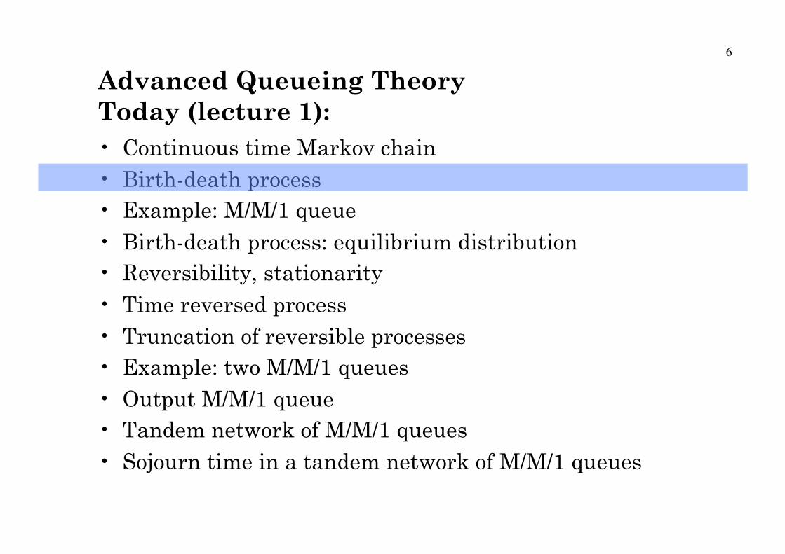
6

Advanced Queueing Theory Today (lecture 1): •  Continuous time Markov chain •  Birth-death process •  Example: M/M/1 queue •  Birth-death process: equilibrium distribution •  Reversibility, stationarity •  Time reversed process •  Truncation of reversible processes •  Example: two M/M/1 queues •  Output M/M/1 queue •  Tandem network of M/M/1 queues •  Sojourn time in a tandem network of M/M/1 queues

7

Birth-death process

•  State space •  Markov chain, transition rates

•  Kolmogorov forward equations

•  Global balance equations

8


9 M/M/1 queue

•  Poisson arrival process rate , single server, exponential service times, mean 1/

•  State space S={0,1,2,…} •  Markov chain? •  Assume initially empty: P(X(0)=0)=1,

•  Transition rates :

€

λ

€

µ

10 M/M/1 queue

•  Kolmogorov forward equations, j>0

•  Global balance equations, j>0

11

M/M/1 queue

j j+1

Equilibrium distribution: <

Stationary measure; summable equilibrium distribution Proof: Insert into global balance Detailed balance!

Theorem: A distribution that satisfies detailed balance is a stationary distribution

€

λ

€

µ

€

λ

€

µ

12


13 Birth-death process •  State space •  Markov chain, transition rates

•  Definition: Detailed balance equations

•  Theorem: Assume that

then

is the equilibrium distrubution of the birth-death process X.

14


15 Reversibility; stationarity •  Stationary process: A stochastic process is stationary if

for all t1,…,tn,

•  Theorem: If the initial distribution of a Markov chain is a stationary distribution, then a Markov chain is stationary

•  Reversible process: A stochastic process is reversible if for all t1,…,tn,

€

τ

€

τ

16 Reversibility; stationarity

•  Lemma: A reversible process is stationary.

•  Theorem: A stationary Markov chain is reversible if and only if there exists a collection of positive numbers π(j), j S, summing to unity that satisfy the detailed balance equations

When there exists such a collection π(j), j S, it is the equilibrium distribution.

•  Proof

€

∈

€

∈

17 Proof

suppose process reversible Let

rev.:

then

Conversely: suppose there exists π satisfying detailed balance, summing gives global balance.

18 Proof (ctd.)

Consider behaviour of X(t) for -T≤t ≤T starts at –T in j1, stays random time h1 before jumping to j2, stays random time h2, before jumping to j3, and so on, until it arrives at jm, where it stays until T Probability density for this path is

density with respect to h1,…hm. Integrate over h1,…hm such that h1+…+hm=2T.

Detailed balance implies

so that (*) is prob density for path starting –T in jm, stays random time hm before jumping to jm-1, and so on, until it arrives at j1, stays until T.

Thus, also invoking stationarity,

(*)

19

Kolmogorov’s criteria

•  Theorem: A stationary Markov chain is reversible iff

for each finite sequence of states.

Furthermore,

for each sequence for which the denominator is positive.

20


21 Time reversed process •  X(t) reversible Markov process X(-t) also, but time

homogeneity not inherited for non-stationary process

•  Lemma: If X(t) is a time-homogeneous Markov process which is non stationary, then the reversed process X( -t) is a Markov process which is not even time-homogeneous.

•  Proof. X(t) is a Markov process X( -t) easy non-time-homogeneous: observe

does not depend on t (time-hom) do depend on t at least for some t,j,k and so also the transition probabilities of the reversed process

€

τ

€

τ

22 Time reversed process

•  Theorem: If X(t) is a stationary Markov process with transition rates q(j,k), and equilibrium distribution π(j), j S, then the reversed process X( - t) is a stationary Markov process with transition rates

and the same equilibrium distribution.

•  Theorem: Kelly’s lemma Let X(t) be a stationary Markov process with transition rates q(j,k). If we can find a collection of numbers q’(j,k) such that q’(j)=q(j), j S, and a collection of positive numbers (j), j S, summing to unity, such that

then q’(j,k) are the transition rates of the time-reversed process, and (j), j S, is the equilibrium distribution of both processes.

€

τ

€

∈

€

∈

€

∈ €

∈

€

π €

π

23


24

Theorem: If the transition rates of a reversible Markov process with state space S and equilibrium distribution are altered by changing q(j,k) to cq(j,k) for where c>0, then the resulting Markov process is reversible in equilibrium and has equilibrium distribution B is the normalizing constant.

If c=0 then the reversible Markov process is truncated to A and the resulting Markov process is reversible with equilibrium distribution

Truncation of reversible processes

A

S\A

25


26 Example: two M/M/1 queues

•  Consider two M/M/1 queues, queue i with Poisson arrival process rate i, service rate i

•  Independence:

•  Now introduce a common capacity restriction

•  Queues no longer independent, but

€

π ( j1, j2 ) =i=1

2

∏ (1− ρi)ρiji , , j1, j2 ≥ 0 ,ρi = λ /µi <1

j1 + j2 ≤ J

π ( j1, j2 ) = Bi=1

2

∏ (1− ρi)ρiji , , j1, j2 ≥ 0, j1 + j2 ≤ J

1

2

€

µ

€

λ

27


28 Output M/M/1 queue: Burkeʼs theorem

•  M/M/1 queue, Poisson( ) arrivals, exponential( ) service

•  X(t) number of customers in M/M/1 queue:

in equilibrium reversible Markov process.

•  Forward process: upward jumps Poisson ( )

•  Reversed process X(-t): upward jumps Poisson ( )

= downward jump of forward process

•  Downward jump process of X(t) Poisson ( ) process

€

λ

€

λ

€

λ

€

λ

€

µ

29 Output M/M/1 queue (2)

•  Let t0 fixed. Arrival process Poisson, thus arrival process after t0 independent of number in queue at t0.

•  For reversed process X(-t): arrival process after –t0 independent of number in queue at –t0

•  Reversibility: joint distribution departure process up to t0 and number in queue at t0 for X(t) have same distribution as arrival process to X(-t) up to –t0 and number in queue at –t0.

•  Burkes theorem: In equilibrium the departure process from an M/M/1 queue is a Poisson process, and the number in the queue at time t0 is independent of the departure process prior to t0

•  Holds for each reversible Markov process with Poisson arrivals as long as an arrival causes the process to change state

30


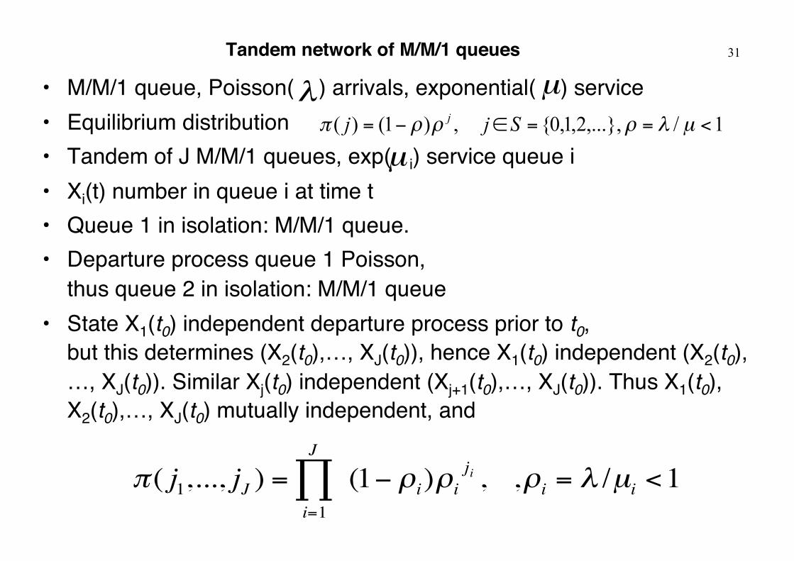
31 Tandem network of M/M/1 queues

•  M/M/1 queue, Poisson( ) arrivals, exponential( ) service

•  Equilibrium distribution •  Tandem of J M/M/1 queues, exp( i) service queue i •  Xi(t) number in queue i at time t •  Queue 1 in isolation: M/M/1 queue. •  Departure process queue 1 Poisson,

thus queue 2 in isolation: M/M/1 queue •  State X1(t0) independent departure process prior to t0,

but this determines (X2(t0),…, XJ(t0)), hence X1(t0) independent (X2(t0),…, XJ(t0)). Similar Xj(t0) independent (Xj+1(t0),…, XJ(t0)). Thus X1(t0), X2(t0),…, XJ(t0) mutually independent, and

€

π ( j1,..., jJ ) =i=1

J

∏ (1− ρi)ρiji , ,ρi = λ /µi <1

€

λ

€

µ

€

µ

32

Example: feed forward network of M/M/1 queues

€

π ( j1,..., j5 ) =i=1

5

∏ (1− ρi)ρiji , ,ρi = λi /µi <1

1

2

4

3

5

33


34 Waiting time M/M/1 queue (1)

•  Consider simple queue FCFS discipline –  W : waiting time typical customer in M/M/1

(excludes service time) –  N customers present upon arrival –  Sr (residual) service time of customers present PASTA

Voor j=0,1,2,…

35 Waiting time M/M/1 queue (2)

•  Thus

•  is exponential ( )

€

µ − λ

36

•  Recall: In equilibrium the departure process from an M/M/1 queue is a Poisson process, and the number in the queue at time t0 is independent of the departure process prior to t0

•  Theorem: If service discipline at each queue in tandem of J M/M/1 queues is FCFS, then in equilibrium the waiting times of a customer at each of the J queues are independent

•  Proof: Kelly p. 38

•  Tandem M/M/s queues: overtaking

Sojourn time tandem M/M/1 queues

37

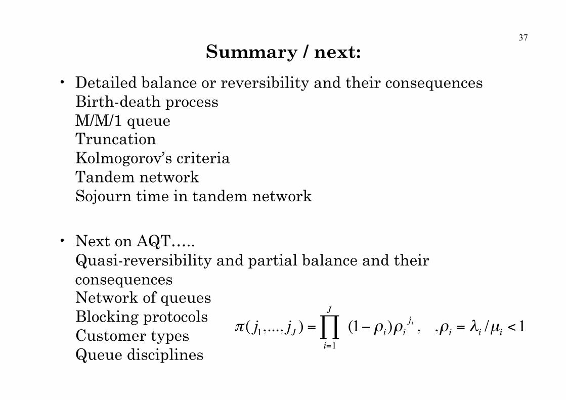
Summary / next:

•  Detailed balance or reversibility and their consequences Birth-death process M/M/1 queue Truncation Kolmogorov’s criteria Tandem network Sojourn time in tandem network

•  Next on AQT….. Quasi-reversibility and partial balance and their consequences Network of queues Blocking protocols Customer types Queue disciplines

€

π ( j1,..., jJ ) =i=1

J

∏ (1− ρi)ρiji , ,ρi = λi /µi <1

Documents

Advanced Queueing Theory