Real Economic Shocks and Sovereign Credit Risk∗Forthcoming, Journal of Financial and Quantitative Analysis

Patrick Augustin† Romeo Tedongap‡

McGill University Stockholm School of Economics

Abstract

We provide new empirical evidence that U.S. expected growth and consumption

volatility are closely related to the strong co-movement in sovereign spreads. We ra-

tionalize these findings in an equilibrium model with recursive utility for CDS spreads.

The framework nests a reduced-form default process with country-specific sensitivity to

expected growth and macroeconomic uncertainty. Exploiting the high-frequency infor-

mation in the CDS term structure across 38 countries, we estimate the model and find

parameters consistent with preference for early resolution of uncertainty. Our results

confirm the existence of time-varying risk premia in sovereign spreads as compensation

for exposure to common U.S. macroeconomic risk.

Keywords: CDS, Generalized Disappointment Aversion, Sovereign Risk, Term StructureJEL Classification: C5, E44, F30, G12, G15

∗The authors would like to thank the Managing Editor Stephen J. Brown and an anonymous referee fortheir valuable inputs to this draft of the paper. We would also like to thank David Backus, Steven Baker,Nina Boyarchenko, Tobias Broer, Anna Cieslak, Mike Chernov, Magnus Dahlquist, Rene Garcia, JørgenHaug, Kris Jacobs, David Lando, Belen Nieto, Stijn Van Nieuwerburgh, Paoloa Zerilli, Stanley Zin andseminar participants at the Stockholm School of Economics, the London School of Economics AIRC, theIRMC Amsterdam, the Nordic Finance Network, the EDHEC Business School, the Bank of Spain/Bankof Canada Workshop on Advances in Fixed Income Modeling, the New York Fed, the NYU Stern Macro-Finance Workshop, the Queen Mary University London, the 2012 Meeting of the Econometric Society, the2012 Financial Econometrics Conference in Toulouse, the European Economic Association 2012 Malaga,the 3rd International Conference of the Financial Engineering and Banking Society in Paris and the 2013Northern Finance Association for helpful comments. The present project has been supported by the NationalResearch Fund Luxembourg, the Nasdaq-OMX Nordic Foundation, the Jan Wallander and Tom HedeliusFoundation, as well as the Bank Research Institute in Stockholm.†McGill University - Desautels Faculty of Management, 1001 Sherbrooke St. West, Montreal, Quebec

H3A 1G5, Canada. Email: Patrick.Augustin@mcgill.ca.‡Swedish House of Finance and Stockholm School of Economics, Drottninggatan 98, SE-111 60 Stockholm,

Sweden. Email: Romeo.Tedongap@hhs.se.

I Introduction

Sovereign credit spreads co-move significantly over time. In light of this fact, there is sub-

stantial evidence that global factors have strong explanatory power for sovereign credit risk

(in particular at higher frequencies), above and beyond that of country-specific fundamen-

tals. The recent literature has emphasized the United States (U.S.) financial channel as

a global source of risk (Pan and Singleton (2008), Longstaff, Pan, Pedersen, and Singleton

(2010)). Whether the ultimate source is financial or macroeconomic in nature is nevertheless

a debate (Ang and Longstaff (2013)).1 We emphasize the macroeconomic channel through

new empirical evidence on a tight relationship of expected U.S. consumption growth and

consumption volatility with sovereign credit risk. We rationalize this evidence by embedding

a reduced-form default process driven by expected growth and consumption volatility into

an equilibrium model for credit default swap (CDS) spreads. The model’s ability to match

several dimensions of the sovereign CDS market corroborates the existence of time-varying

risk premia as compensation for exposure to (common) U.S. macroeconomic risk.

We empirically document a strong association between sovereign and global macroeco-

nomic risk, which cannot be accounted for by global financial risk. To demonstrate our re-

sults, we exploit the homogenous contract specification and daily variation in CDS spreads.2

Our sample contains information on the full term structure for a geographically dispersed

panel of 38 countries. The motivation for our analysis is based on the fact that sovereign

defaults tend to cluster at business cycle frequencies (Reinhart and Rogoff (2008)). First, we

show that the average level of spreads has a surprisingly high correlation of respectively -65%

and 85% with expected growth rates and economic uncertainty in the U.S. Second, the same

two risk factors in turn can account for approximately 75% of the variation in the first two

common factors embedded in the term structure across all 38 countries. We believe the two

1Ang and Longstaff (2013) focus on systemic sovereign risk.

2CDS spreads are better comparable across countries than sovereign bonds, as they are not plagued by

differences in covenants, issuer country legislation or declining spread maturities.

1

factors to be a level and a slope factor. Importantly, this association is robust against a bat-

tery of financial market variables, such as the CBOE S&P 500 volatility index, the variance

risk premium, the U.S. excess equity return, the price-earnings ratio as well as the high-yield

and investment-grade bond spreads. While some of these factors have individually statistical

explanatory power for the level factor, none of them accounts for the variation in the slope

factor. Third, we document that our results are qualitatively and quantitatively maintained

for country-specific regressions, where we test for the level and slope of the CDS term struc-

ture as regressands. The empirical evidence survives several robustness tests, among which

one suggests that expected growth and consumption volatility contemporaneously predict

the Reinhart and Rogoff sovereign distress indicator over the past 50 years.

These new empirical findings suggest that consumption risks are priced factors in the

term structure of sovereign CDS spreads and that time-variation in expected growth and

consumption volatility are strongly related to the significant co-movement in spreads. We

rationalize this result through a general equilibrium framework for CDS spreads that embeds

a reduced-form default process driven by aggregate consumption risk factors. Our rational

investor is risk averse and exhibits Epstein and Zin (1989) (EZ) recursive preferences. We also

extend the model to accommodate generalized disappointment averse (GDA) preferences as

in Routledge and Zin (2010). The conditional mean and volatility of aggregate consumption

growth, the two state variables of our endowment economy, drive the default process, while

countries differ cross-sectionally through their sensitivity to the systematic risk factors. As

the model yields closed-form solutions for CDS spreads and their moments, we are able

to estimate the structural parameters of the model. In addition, country spreads can be

interpreted based on preferences and exposures to macroeconomic risk factors.

To investigate the asset pricing implications, we exploit the high-frequency information

in CDS spreads from May 2003 through August 2010 and estimate both preference param-

eters and the cross-sectional default sensitivities to expected growth rates and consumption

volatility. We quantitatively match the unconditional mean, volatility, skewness and persis-

2

tence of the term structure, the decreasing pattern of the kurtosis with asset maturity as well

as historically observed cumulative default probabilities. A two-factor model for the default

process is necessary to account for these stylized facts, as a specification based only on ex-

pected consumption growth consistently produces a term structure, which is too steep, while

it is too low if macroeconomic uncertainty is the only source of risk. Adding country-specific

shocks to the model only marginally improves the fit. In addition to average upward sloping

term structures, the model qualitatively matches the conditional slope reversals for distressed

sovereign borrowers in states of bad macroeconomic fundamentals. Both the EZ and GDA

scenarios produce comparable unconditional results. However, a model with downside risk

aversion endogenously generates relatively higher risk aversion in states of bad macroeco-

nomic fundamentals, which yields a stronger term structure inversion in the worst economic

state that is quantitatively consistent with empirically observed magnitudes. A likelihood

ratio test favors asymmetric preferences over symmetric gambles. State-dependent prices

in bad states further reflect the tail risk embedded in CDS spreads. Moreover, the model

produces ratios of risk-neutral to physical default probabilities consistent with the literature.

Regarding the preference parameters in the EZ (GDA) case, we estimate an elasticity

of intertemporal substitution of 1.58 (1.49) and a coefficient of relative risk aversion of 8.27

(4.91), consistent with preference for early resolution of uncertainty. In the GDA case, we

estimate a disappointment aversion parameter of 0.25 and a disappointment threshold at 85%

of the certainty equivalent. We continue to match first and second moments of the stock

market and risk-free rate. We thus provide a joint framework for pricing equity and fixed

income derivatives, consistent with evidence of information flow between both markets.3

The results suggest that a simple two-factor model including expected growth and macroe-

conomic uncertainty is sufficient to explain a large fraction of the common time-variation

in the global sovereign CDS market. While the previous literature has emphasized the im-

3Two recent papers addressing the equity and cash credit spread puzzle in a unified consumption-based

framework are Bhamra, Kuehn, and Strebulaev (2010) and Chen, Collin-Dufresne, and Goldstein (2009).

3

portance of U.S. financial market variables for the common variation in spreads (Pan and

Singleton (2008), Longstaff, Pan, Pedersen, and Singleton (2010), Ang and Longstaff (2013)),

we focus on a different channel: shocks to the expected level and volatility of U.S. consump-

tion growth. We explain our findings in a tractable two-state model.4 Surprisingly, Pan

and Singleton (2008) address the importance of consumption risk in their discussion, yet

don’t include it directly in their analysis. Other evidence on the role of global factors in

explaining the co-movement in sovereign spreads points to links through U.S. interest rates

(Uribe and Yue (2006)), investors’ risk appetite (Baek, Bandopadhyaya and Du (2005), Re-

molona, Scatigna, and Wu (2008), Gonzalez-Rozada and Yeyati (2008)), investor sentiment

(Weigel and Gemmill (2006)), aggregate credit risk (Geyer, Kossmeier, and Pichler (2004))

or contagion (Benzoni, Collin-Dufresne, Goldstein, and Helwege (2012)).

Benzoni, Collin-Dufresne, Goldstein, and Helwege (2012) develop an equilibrium model

for CDSs with fragile beliefs as in Hansen (2007) and Hansen and Sargent (2010). The

co-movement in spreads arises through a hidden contagion factor that affects the posterior

default distribution of all countries after a shock to one individual country. They focus on

fitting the dynamics of the level of spreads, while we show that a simple two-factor model

matches higher order moments of the term structure. Our model is conceptually also close

to Borri and Verdelhan (2009), who apply the Campbell and Cochrane (1999) external habit

framework to show that emerging market bonds reflect a risk premium for exposure to the

U.S. market returns. Their objective is closer to the extensive literature on the sovereign

incentives to default and they fail to match the level of spreads. We focus on the pricing

of spreads and match the moments of the term structure up to the fourth order closely.

Moreover, we derive analytic solutions for non-linear CDS payoffs, allowing us to estimate

the default and preference parameters in the model.

We believe our results to be useful in better understanding the determinants of the

4The consumption correlation puzzle of Backus, Kehoe, and Kydland (1992) illustrates that consumption

growth is only weakly correlated across countries.

4

term structure of sovereign credit risk. Improving this understanding is warranted in light

of the developments in the emerging markets in the nineties, and particularly the recent

sovereign debt crisis in Europe with six international bailouts in approximately three years.

Understanding the relationship between higher frequency variation in sovereign spreads and

global risk factors is also relevant for the diversification benefits of international investors

and the efficiency of government intervention aimed at reducing sovereign borrowing costs.

The rest of the paper proceeds as follows. Section 2 provides new empirical evidence on

a tight link between sovereign credit and aggregate macroeconomic risk. Section 3 presents

the general equilibrium framework for CDS spreads. The model estimation is explained in

section 4, followed by a discussion of the results in section 5. We conclude in section 6.

II U.S. Consumption Risk and Sovereign CDS Spreads

Reinhart and Rogoff (2008) document over a 200-year period that sovereign defaults tend to

cluster at business-cycle frequencies. This motivates us to investigate more closely the link

between sovereign credit risk, for which we exploit the daily information on sovereign distress

embedded in CDS spreads, and global macroeconomic risk, proxied through the conditional

mean and volatility of aggregate U.S. consumption growth. The next paragraph describes

our CDS dataset, followed by a deeper study of its link with global macroeconomic risk.

A CDS Data and Summary Statistics

A CDS is a fixed income derivative, which allows a protection buyer to purchase insurance

from the protection seller against a contingent credit event on a reference entity by paying

a premium, referred to as the CDS spread.5 CDSs are particularly useful to study sovereign

credit risk across countries as the contract specification is identical for each sovereign. Pub-

lic bonds are usually characterized through differences in covenants and are often issued in

5Pan and Singleton (2008) describe the structure and institutional details of the sovereign CDS market.

5

different legal jurisdictions. In addition, CDSs are constant-maturity products with price in-

formation available at daily frequencies. This makes them suitable for studying the common

variation in sovereign spreads, which is particularly pronounced at higher frequencies.

Our data set consists of daily mid composite USD denominated CDS prices for 38

sovereign countries from Markit over the sample period May 9th, 2003 until August 19th,

2010, and covers prices for the full term structure, including 1, 2, 3, 5, 7 and 10-year con-

tracts.6,7 All contracts contain the full restructuring clause. The sample is representative

of the global sovereign CDS market as it spans 4 major geographical regions and 17 rating

categories. The list of 38 countries is provided in Table 1. Keeping track of rating changes

over time, there are on average 4 countries in rating category AAA, 6 in AA, 9 in A, 11 in

BBB, 6 in BB and 2 in rating group B.8

Our working data set thus contains 1900 observations for 38 countries and 6 maturities,

amounting to a total of 433,200 observations. We aggregate countries by rating categories

and present summary statistics in Table 2.9 The dataset exhibits a considerable amount of

heterogeneity both across time and across countries. For instance, the mean 5-year spread for

AAA rated countries is 22 basis points and 558 basis points for B rated sovereigns. The mean

term structure is always upward sloping, increasing monotonically with the deterioration of

credit quality from 11 (AAA) to 177 basis points (B). The sample features great time-series

variation, with standard deviations for the 5-year series ranging from 31 (AAA) to 287

basis points (B). All time series are highly persistent, with an average daily autocorrelation

coefficient for 5-year spreads as high as 0.9965.

6We fill gaps with CDS information from CMA Datastream and interpolate if no information is available.

7While trading in corporate CDS is highly concentrated around the 5-year maturity, Pan and Singleton

(2008) document that trading volume in sovereign CDS is more balanced across maturities.

8Venezuela is excluded for the 31 first days of the sample period when it was rated CCC+.

9We map ratings into a numerical scheme ranging from 1 (AAA) to 21 (C). The daily rating-specific

spread is the equally weighted mean spread of countries in a rating group.

6

B The Role of Macroeconomic Risk

As a first exercise to investigate the relationship between sovereign and global macroeconomic

risk, we test how strongly U.S. consumption risk factors are related to the common factors

in the sovereign CDS term structure. A principal component analysis (PCA) on the level

of spreads yields that the first two factors account for approximately 91% of the common

variation. This is rather strong, given the wide spectrum of contract maturities and reference

entities we consider. The magnitude is consistent with Pan and Singleton (2008), who

find that the first principal component explains on average 96% of the (daily) common

variation for Korea, Turkey and Mexico, and Longstaff, Pan, Pedersen, and Singleton (2010),

who document an average explained (monthly) variation by the first factor of 64% for 26

countries, increasing to 75% during the financial crisis. Table 3 illustrates the proportion

of the variance explained by the first six principal components. The magnitudes remain

similar for subsamples of the term structure. The importance of the first factor decreases

nevertheless relative to the second factor as we move towards longer maturities.

To summarize the information from the PCA, we average the country factor loadings

across maturities. Figure 1 shows that the average factor loadings on the first principal

component have roughly equal magnitudes, whereas those on the second factor increase

monotonically with maturity. We therefore interpret the first and second factors as a level

and slope factor in the CDS term structure.

If U.S. consumption risk is priced in the sovereign CDS market, then it ought to be linked

to the factors extracted from this PCA. As insurance premia on contingent future default

events may be linked to expectations about future growth rates, we investigate both channels

of time-varying expected consumption growth and macroeconomic uncertainty. More specif-

ically, we use monthly real per capita consumption data from January 1959 until August

7

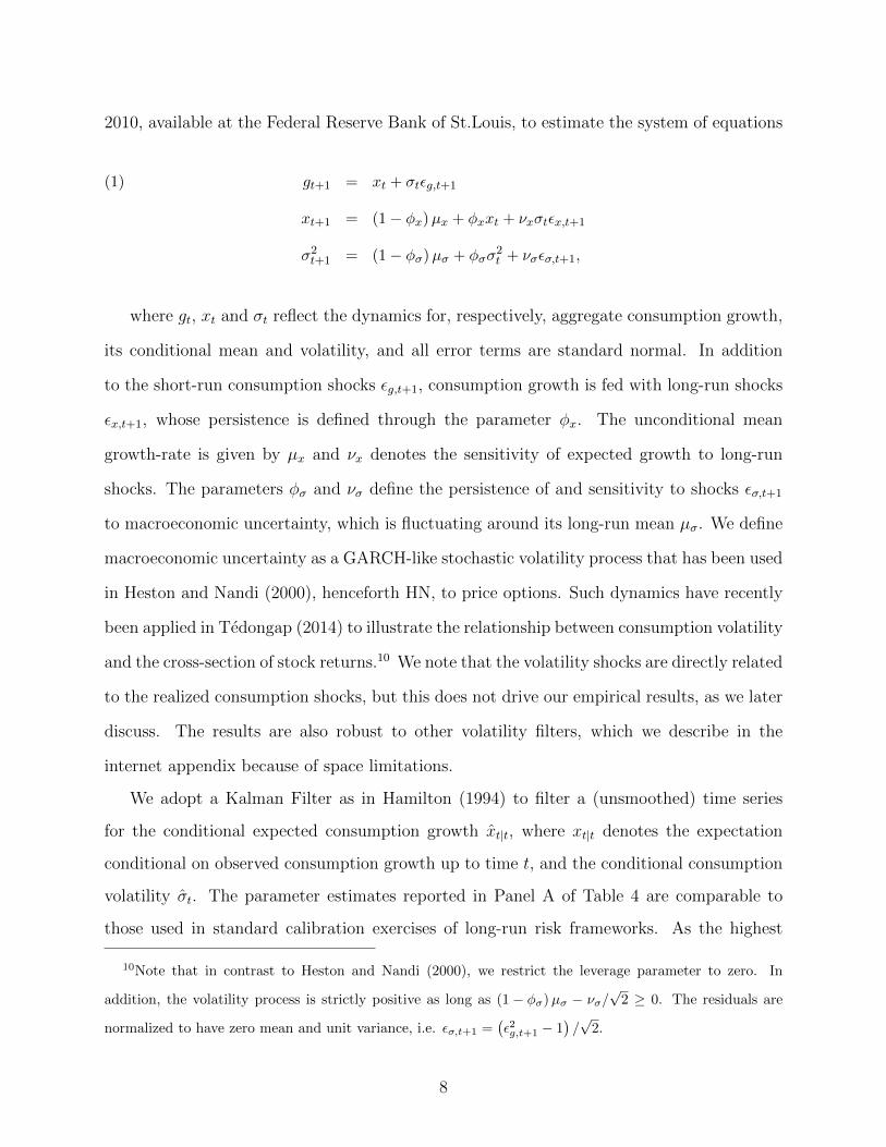
2010, available at the Federal Reserve Bank of St.Louis, to estimate the system of equations

gt+1 = xt + σtεg,t+1(1)

xt+1 = (1− φx)µx + φxxt + νxσtεx,t+1

σ2t+1 = (1− φσ)µσ + φσσ

2t + νσεσ,t+1,

where gt, xt and σt reflect the dynamics for, respectively, aggregate consumption growth,

its conditional mean and volatility, and all error terms are standard normal. In addition

to the short-run consumption shocks εg,t+1, consumption growth is fed with long-run shocks

εx,t+1, whose persistence is defined through the parameter φx. The unconditional mean

growth-rate is given by µx and νx denotes the sensitivity of expected growth to long-run

shocks. The parameters φσ and νσ define the persistence of and sensitivity to shocks εσ,t+1

to macroeconomic uncertainty, which is fluctuating around its long-run mean µσ. We define

macroeconomic uncertainty as a GARCH-like stochastic volatility process that has been used

in Heston and Nandi (2000), henceforth HN, to price options. Such dynamics have recently

been applied in Tedongap (2014) to illustrate the relationship between consumption volatility

and the cross-section of stock returns.10 We note that the volatility shocks are directly related

to the realized consumption shocks, but this does not drive our empirical results, as we later

discuss. The results are also robust to other volatility filters, which we describe in the

internet appendix because of space limitations.

We adopt a Kalman Filter as in Hamilton (1994) to filter a (unsmoothed) time series

for the conditional expected consumption growth xt|t, where xt|t denotes the expectation

conditional on observed consumption growth up to time t, and the conditional consumption

volatility σt. The parameter estimates reported in Panel A of Table 4 are comparable to

those used in standard calibration exercises of long-run risk frameworks. As the highest

10Note that in contrast to Heston and Nandi (2000), we restrict the leverage parameter to zero. In

addition, the volatility process is strictly positive as long as (1− φσ)µσ − νσ/√

2 ≥ 0. The residuals are

normalized to have zero mean and unit variance, i.e. εσ,t+1 =(ε2g,t+1 − 1

)/√

2.

8

available frequency for consumption information is monthly, we regress monthly averages of

the first two factor scores Fi,t onto conditional expected growth and consumption volatility

Fi,t = a0,i + a1,i × xt|t + a2,i × σt + εt,(2)

where i = 1, 2 and t is the month index. Results based on 88 monthly observations with

block-bootstrapped standard errors are reported in columns (1) to (2) of Table 5.

Both coefficients on the explanatory variables are statistically significant at the 1% sig-

nificance level for regressions (1) and (2). In addition, the adjusted R2 from the first two

regressions is 75% and 74%, respectively. On a stand-alone basis, U.S. consumption risk

seems strongly associated with the first two common components in the CDS term struc-

ture, which themselves explain on average almost 91% of the time-variation in sovereign

spreads. We will discuss the signs of the individual regression coefficients in relation to the

model-implied results on the assumption that the first two principal components reflect a

level and a slope factor. An exact interpretation of the economic magnitudes of the latent

factor loadings in relation to the common factors is, however, more difficult.

Our results support the view that expected U.S. consumption growth and volatility are

two risk factors in the term structure of sovereign credit spreads.11 Macroeconomic shocks

channel through to the level and the slope of the term structure. A back-of-the-envelope

calculation yields that shocks to expected U.S. consumption growth and volatility manage to

explain roughly 68.25% of the common variation in sovereign CDS premia.12 Our conclusion

is visually emphasized by plotting the filtered series of conditional expected consumption

growth and consumption volatility against the average monthly 5-year CDS spread of all 38

countries in Figure 2. There is a strong negative correlation (-65%) between the average

11We acknowledge an error-in-variables problem in the factor regressions, but a simultaneous estimation

of the regression coefficients and the risk factors is unlikely to undo our strong results.

12This back-of-the-envelope calculation is based on the filtered consumption series, which explains 75%

of the first two principal components, which themselves account for 91% of the variation in spreads.

9

sovereign spread and conditional expected consumption growth. Moreover, the conditional

consumption volatility tracks the mean 5-year CDS spread closely with a staggering corre-

lation of 85%.

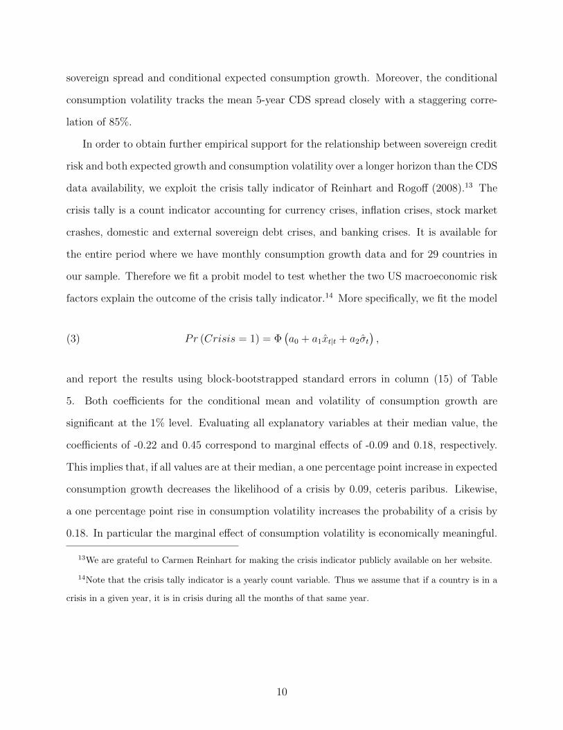
In order to obtain further empirical support for the relationship between sovereign credit

risk and both expected growth and consumption volatility over a longer horizon than the CDS

data availability, we exploit the crisis tally indicator of Reinhart and Rogoff (2008).13 The

crisis tally is a count indicator accounting for currency crises, inflation crises, stock market

crashes, domestic and external sovereign debt crises, and banking crises. It is available for

the entire period where we have monthly consumption growth data and for 29 countries in

our sample. Therefore we fit a probit model to test whether the two US macroeconomic risk

factors explain the outcome of the crisis tally indicator.14 More specifically, we fit the model

Pr (Crisis = 1) = Φ(a0 + a1xt|t + a2σt

),(3)

and report the results using block-bootstrapped standard errors in column (15) of Table

5. Both coefficients for the conditional mean and volatility of consumption growth are

significant at the 1% level. Evaluating all explanatory variables at their median value, the

coefficients of -0.22 and 0.45 correspond to marginal effects of -0.09 and 0.18, respectively.

This implies that, if all values are at their median, a one percentage point increase in expected

consumption growth decreases the likelihood of a crisis by 0.09, ceteris paribus. Likewise,

a one percentage point rise in consumption volatility increases the probability of a crisis by

0.18. In particular the marginal effect of consumption volatility is economically meaningful.

13We are grateful to Carmen Reinhart for making the crisis indicator publicly available on her website.

14Note that the crisis tally indicator is a yearly count variable. Thus we assume that if a country is in a

crisis in a given year, it is in crisis during all the months of that same year.

10

C Macroeconomic vs. Financial Risk

The previous empirical findings highlight the possibility that expected growth and macroeco-

nomic uncertainty may explain the co-movement of sovereign CDS spreads. Previous papers

have identified a link between sovereign risk premia and financial market variables such as the

variance risk premium (Wang, Zhou, and Zhou (2010)) or the CBOE S&P500 volatility index

(Pan and Singleton (2008), Longstaff, Pan, Pedersen, and Singleton (2010)). An alternative

explanation to our story would be that, as financial volatility increases, risk-averse investors

adjust their consumption patterns to account for future macroeconomic uncertainty. We

explore this hypothesis in three ways.

First, we rerun the factor regressions of equation (2) by projecting the first two factors

from the PCA on several global financial market variables such as the variance risk premium

(VRP), the CBOE S&P500 volatility index (VIX), the monthly excess value-weighted return

on all NYSE, AMEX, and NASDAQ stocks from CRSP (USret), the US price-earnings ratio

(PE), as well the difference between the Bank of America/Merrill Lynch BBB and AAA

effective yield (IG) and the difference between the BB and BBB effective yield (HY).15 We

then run a horse race with the global macroeconomic risk factors and test the robustness of

the probit specification in equation (3) against the inclusion of financial market variables.

The univariate regressions are reported in columns (3) to (14) of Table 5. Only the

coefficients for VIX, PE, IG and HY are statistically significant on their own for the first

common factor and, assuming it reflects a level factor, have economically plausible signs.

None of the coefficients are statistically significant for the second principal component.16

Moreover, for the first factor regression, the adjusted R2 of the VIX is with 55% significantly

smaller than the 75% obtained with the macroeconomic risk factors and the PE, IG and HY

have adjusted R2s in the same ballpark region. Most importantly though, for the second

15The data for the VRP is taken from Hao Zhou’s webpage, the USret from Kenneth French’s website,

the PE from Robert Shiller’s website, and the VIX, AAA BBB and BBB BB from the FRED H15 report

16Only PE is borderline significant at the 5% level.

11

factor regression, the maximum adjusted R2 of 9% is obtained for PE (4% for IG and 2% for

HY), compared to 74% for the conditional mean and volatility of US consumption growth.

A horse race between macroeconomic and financial risk confirms the former’s importance

for the common factors in the term structure of sovereign CDS spreads. Columns (1) to

(12) of Table 6 show that none of the financial market variables drives out the statistical

significance of expected growth and macroeconomic uncertainty. Again, only the PE, IG

and HY remain statistically significant for the first factor and none of them has statistical

significance for the second factor. Importantly, the sign of consumption volatility is always

preserved and changes little in magnitude. Comparing all variables in columns (13) and (14),

only the high-yield spread keeps its statistical significance at the 5% level for the level factor,

while the consumption risk factors remain highly statistically significant for both the level

and slope factors.17 Thus, our results suggest that only the high-yield bond spread (HY)

contains additional information besides the macroeconomic risk factors for the level factor

in the term structure of sovereign CDS spreads, while global financial risk has no additional

explanatory power beyond the conditional mean and volatility of consumption growth for the

slope factor. Finally, we include in column (16) of Table 5 the USret and PE into the probit

regressions as they are available since 1959. The results are qualitatively and quantitatively

maintained. In column (17), we use all financial market variables over a shorter time period

starting in 1996 and we include all countries from the Reinhart & Rogoff database. Over

the shorter time period, the coefficient of consumption volatility of 0.99 corresponds to a

marginal effect of 0.38, implying that a one percentage point rise in consumption volatility

increases the probability of a crisis by 0.38. Overall, these results corroborate our hypothesis

of U.S. macroeconomic fundamentals being a source of common sovereign credit risk.

17The coefficient on expected growth flips sign, which is due to multicollinearity issues with the PE ratio

and the investment-grade and high-yield bond spreads. We have tested that the part of expected consumption

growth orthogonal to the other variables remains statistically significant in the horse race regressions with

a negative sign on the level factor. The power and economic sign for the level factor of this orthogonalized

component is on its own interesting, but is not central to our message.

12

To close the loop of our analysis, we regress in Table 7, for each country, empirical

measures of the level and slope of the CDS term structure on the same macroeconomic

and financial risk factors.18 The level of the term structure at any day t is defined as the

average spread over all maturities, the slope is the difference between the 10-year and the

1-year spread.19 Our previous conclusions hardly change. The power of the VRP fades out

once we include the consumption risk factors. At least 58% of the coefficients on xt|t and

σt are statistically significant, while this is the case for maximally 21% of the coefficients

on the VRP. Moreover, the median adjusted R2s are high, ranging from 54% for the slope

regressions up to 70% for the level regressions. The signs of the coefficients are consistent with

the evidence of countercyclical spreads and default probabilities. A rise in expected growth

decreases the level of spreads for 68% of all countries, whereas a rise in macroeconomic

uncertainty raises the level of spreads for 97% of all countries. On the other hand, the

term structure loads positively on expected growth for more than half of all countries, and

positively on macroeconomic uncertainty for 74% of all countries in the univariate regressions.

A concern is that the level and slope measures are highly correlated. To the contrary, the

correlation between the level and slope is a weak 12%.

To summarize, our results show that global macroeconomic risk contains information un-

accounted for by financial market variables for the first two common factors in the sovereign

CDS term structure. These new findings motivate us to develop a parsimonious preference-

based model for sovereign CDSs using only two state variables, time-varying expected growth

and consumption volatility.

18We report and discuss only results for the VRP.

19Alternatively, we tried the 5-year CDS spread as a measure of the level. Results hardly change.

13

D Robustness of the Empirical Results

In order to strengthen the empirical evidence of a relationship between global macroeco-

nomic and sovereign credit risk, we conduct several robustness tests.20 First, we run the

regressions in first differences rather than in levels. Second, we discuss the use of industrial

production growth data as an alternative to consumption growth. Third, we check alterna-

tive specifications of the endowment dynamics. Fourth, we check whether our results are

robust to the inclusion of realized consumption growth. Finally, we test the relationship

between macroeconomic and financial risk in a VAR specification.

We emphasize that our analysis focuses on spread levels rather than differences, which is

consistent with Doshi, Ericsson, Jacobs, and Turnbull (2013) and references therein.21 As the

authors point out, there is no consensus in the literature, but economic intuition suggests that

spreads are mean-reverting and stationary, as opposed to trending stock prices. In addition,

first differencing comes at the cost of less efficient statistical estimates, and measurement

errors may reduce the signal-to-noise ratio more for difference regressions. We therefore

advocate the use of levels. Irrespectively of our motivation though, a concern may be that the

results are spurious because of high persistence in spreads, expected growth and consumption

volatility. Therefore, we have reported results using difference regressions in section A-V of

the internet appendix. Consistent with the literature, R2 statistics are significantly smaller

for the difference regressions, ranging around 9%. But we maintain statistical significance,

in particular for the regressions with the slope factor. Importantly, we run a Dickey-Fuller

test on the residuals of the regressions in levels and we strictly reject the presence of a unit

root (see last row in Tables 5 and 6). Regressions are thus not spurious. Even if the factors

and consumption variables were integrated of order one, these results would suggest that

there exists a cointegrating relationship. We don’t pursue such tests as they are not the

20We thank an anonymous referee for suggesting several of these robustness checks.

21Campbell and Taksler (2003) use spread levels, and Benzoni, Collin-Dufresne, Goldstein, and Helwege

(2012) advocate regressions in levels.

14

focus of our study. However, if we were to find evidence in favor of a long-run equilibrium

relationship, this would still not undo our message that there exists a strong relationship

between the common information in the term structure of spreads and macroeconomic risk.

Next, we verify our results using monthly industrial production growth data instead of

monthly consumption growth, similar to Bansal, Kiku, Shaliastovich, and Yaron (2013),

Joslin, Le, and Singleton (2013) and Lustig, Roussanov, and Verdelhan (2013). Industrial

production growth data has the advantage of being available since 1919 and correlates sub-

stantially with consumption growth at lower frequencies. Unreported results suggest that

we get statistically significant estimates in the regression analysis with heteroscedasticity-

robust, but not with block-bootstrapped standard errors. We believe that this may be due

to the fact that industrial production, which accounts for inputs and outputs of both non-

durables and durables, is an imperfect proxy for the non-durable component of consumption

growth. At the monthly horizon from 1959 to 2010, the correlation coefficient between the

two time series is only 19.88%.

We further test whether our base regression results are affected by the functional form

specification of consumption volatility. We adopt other GARCH models commonly adopted

in the financial literature: the standard GARCH(1,1) model (Bollerslev (1986)), the EGARCH

model (Nelson (1991)) and the GJR GARCH model (Glosten, Jagannathan, and Runkle

(1993)). The dynamics and parameter estimates of the different GARCH specifications are

reported in Panel B of Table 4. These alternative specifications are comparatively more

persistent, with estimates for φσ ranging from 0.9779 for the GARCH(1,1,) specification to

0.9907 for the EGARCH specification. Replications of the benchmark regression results,

using these different volatility specifications, are reported in section A-VI of the external

internet appendix because of space restrictions. Both the univariate and the multivariate

tests illustrate that a different functional form of the volatility process does not alter our

conclusion of a strong relationship between the first two principal components and expected

consumption growth and volatility.

15

GARCH models inherit contemporaneous correlation between realized consumption growth

and consumption volatility. Hence there is a possibility that large moves in realized con-

sumption growth mechanically lead to large increases in volatility. Therefore we test whether

the significance of the macroeconomic risk factors survives once we control for variation in

realized consumption growth. Unreported results suggest that the statistical relationship

between consumption volatility and the common information in the term structure of CDS

spreads is not merely due to jumps in realized consumption growth. The regression coeffi-

cient on realized consumption growth is insignificant and neither the statistical significance

nor the magnitude of the coefficient on expected growth and consumption volatility changes.

Finally, we investigate the relationship between the macroeconomic risk factors and the

VIX index in a VAR specification. Unreported results show no evidence that financial market

volatility Granger causes expected growth. Moreover, results between consumption volatility

and the VIX are inconclusive and point to mere correlation.

III A Macroeconomic Model for Sovereign CDS

Our empirical exercise highlights that expected U.S. consumption growth and macroeco-

nomic uncertainty accounts for a large fraction of the co-movement in sovereign CDS spreads.

We show that an equilibrium model for CDS spreads with only two state variables can ratio-

nalize these facts. Our ingredients are an endowment economy with time-varying expected

growth and consumption volatility, recursive Epstein and Zin (1989) preferences, and an

embedded reduced-form default process driven by the two state variables of the economy.

A Credit Default Swaps

To derive the valuation of CDS spreads in closed-form, we discretize the continuous frame-

work in Duffie (1999), albeit adapting the explicit modeling of the hazard and recovery rate.

We write the model at a daily frequency in order to agree with daily quotations in the CDS

16

market. We assume that each coupon period n contains J trading days.22 A K-period CDS

thus has KJ trading days. CDSs are priced similar to interest rate swaps, that is expected

net present values of cash flows for both legs (protection buyer and protection seller) must

equalize at inception. For a K-period CDS, the expected net present value of the protection

leg, πpbt , to be paid by the protection buyer is equal to

(4)

πpbt = CDSt (K)

(K∑k=1

Et [Mt,t+kJI (τ > t+ kJ)] + Et

[Mt,τ

(τ − tJ−⌊τ − tJ

⌋)I (τ ≤ t+KJ)

]),

where CDSt (K) is the constant premium agreed at day t and to be paid until the earlier

of maturity (day t + KJ), or a credit event occurring at a random day τ . For t′ > t, Mt,t′

denotes the stochastic discount factor valuing any financial payoff to be claimed at a future

day t′. The floor function b·c rounds a real number to the largest previous integer, and I (·)

is an indicator function taking the value 1 if the condition is met and 0 otherwise. The first

part in equation (4) defines the net present value of payments made by the protection buyer

conditional on survival. The second part defines the accrual payments if the reference entity

defaults between two payment dates.

The protection seller must cover any losses incurred by the protection buyer in case of a

credit event. The expected net present value of the protection seller’s leg, πpst , is equal to

(5) πpst = Et [Mt,τ (1−R) I (τ ≤ t+KJ)] ,

where R represents the constant post-default recovery rate as a fraction of face value, and we

define the constant Loss Given Default L = (1−R).23 We fix the dynamics of the recovery

rate process at a constant level, consistent with industry standards for CDS pricing. This

22Note that the period n contains the trading days (n− 1) J+ j, j = 1, . . . , J . In the calibration exercise,

we assume without loss of generality that swap premia are paid on a yearly basis. The assumption of yearly

payments assures that the model results can directly be translated into annualized spreads. However, the

model can easily accommodate bi-annual and quarterly payment frequencies.

23In what follows, we will interchange freely between the notions of Loss Given Default and Loss Rate.

17

is also in line with standard assumptions in the CDS pricing literature such as Pan and

Singleton (2008) or Longstaff, Pan, Pedersen, and Singleton (2010). We leave the analysis

of time-varying recovery rates for further research.24

Equating the two legs, as the expected net present values are zero at inception, and

applying the Law of Iterated Expectations, we can write the CDS spread as

(6) CDSt (K) =

KJ∑j=1

Et [Mt,t+j (1−R) (St+j−1 − St+j)]

K∑k=1

Et [Mt,t+kJSt+kJ ] +KJ∑j=1

(jJ − b

jJ c)Et [Mt,t+j (St+j−1 − St+j)]

,

where the survival probability St ≡ Prob (τ > t | It) denotes the conditional probability that

the credit event did not occur at day t, and where It denotes the information set up to and

including day t.25 The conditional survival probability St is defined as

St = S0

t∏j=1

(1− hj) , t ≥ 1,(7)

where the hazard rate process ht ≡ Prob (τ = t | τ ≥ t; It) denotes the conditional instanta-

neous default probability of a given reference entity at day t.

To derive analytic solutions to the CDS, we need to specify dynamics for the stochastic

discount factor Mt,t+1 and the default intensity ht+1. These processes are determined by the

two state variables of the economy, which are described in the following section.

B A Markov-switching Model for Consumption Growth

In section II, we estimate the dynamics of consumption growth using a continuous-state

space model because a discrete approximation with regimes does not provide a sufficiently

good approximation in small samples for highly persistent processes such as expected con-

24We did explore the possibility of deterministic procyclical and state-dependent recovery rates, while

keeping the unconditional recovery rate fixed. Our results are not very sensitive to such a variation.

25Note that we assume Prob (τ = t | It′) = Prob(τ = t | Imin(t,t′)

)for all integers t and t′.

18

sumption growth and macroeconomic uncertainty. For the purpose of our model, we do

however approximate the continuous-state dynamics with a discrete regime-switching frame-

work as it is well known that Markov switching models provide excellent approximations of

continuous processes in population (Timmermann (2000), Bonomo, Garcia, Meddahi, and

Tedongap (2011)). More importantly, without the discrete-state approximation, we are not

able to obtain analytical formulas for spread moments in our preference framework, which

is particularly useful for computational efficiency when we want to estimate the preference

parameters. In addition, if we limit us to two regimes for each state variable, the closed-form

formulas enhance the understanding and interpretation of the mechanisms underlying the

empirical results.

Following Bonomo, Garcia, Meddahi, and Tedongap (2011), we assume that both the

mean and variance of consumption growth gt+1 fluctuate according to a Markov variable st,

which can take a different value in each of the N states of the economy. The stochastic

sequence st evolves according to a transition probability matrix P

(8) P> = [pij ]1≤i,j≤N , pij = Prob (st+1 = j | st = i) .

As in Hamilton (1994), let ζt = est , where ej is the N × 1 vector with all components equal

to zero but the jth component equals one. Formally, consumption growth can be written as

(9) gt+1 = xt + σtεg,t+1,

where xt = µ>g ζt and σt =√ω>g ζt are the expected mean and the volatility of consumption

growth respectively. The vectors µg and ωg contain the values of expected consumption

growth and consumption volatility respectively in each state of the economy, and the com-

ponent j refers to the value in state st = j. For simplicity, we limit the number of states to

two for each risk factor, indexed by the letters L for the low state and H for the high states.

This amounts to a total of four states (LL, LH, HL and HH) if the factors are linearly

independent.

19

C Preferences and Stochastic Discount Factor

We study the valuation of CDSs in the context of a representative agent general equilibrium

model. We assume that the representative investor has Epstein and Zin (1989) preferences.

Such an investor derives lifetime utility Vt recursively from the combination of the current

level of consumption Ct and Rt (Vt+1), a certainty equivalent of next period lifetime utility

Vt =

{(1− δ)C

1− 1ψ

t + δ [Rt (Vt+1)]1− 1

ψ

} 1

1− 1ψ if ψ 6= 1(10)

= C1−δt [Rt (Vt+1)]δ if ψ = 1,

where Rt (Vt+1) =(Et[V 1−γt+1

]) 11−γ and where δ represents the subjective discount factor.

The parameter ψ defines the elasticity of intertemporal substitution (EIS), which can be

disentangled from the coefficient of relative risk aversion γ through this form of utility.

Hansen, Heaton, and Li (2008) derive the stochastic discount factor Mt,t+1 in terms of

the continuation value of utility of consumption as

(11) Mt,t+1 = δ

(Ct+1

Ct

)− 1ψ(

Vt+1

Rt (Vt+1)

) 1ψ−γ.

If γ = 1/ψ, equation (11) corresponds to the stochastic discount factor of an investor with

time-separable utility and constant relative risk aversion. Alternatively, if γ > 1/ψ, Bansal

and Yaron (2004), for instance, show that a premium for long-run consumption risk is added

by the ratio of future utility Vt+1 to its certainty equivalent Rt (Vt+1).

Based on the dynamics (9) and the recursion (10), we show in the internet appendix

section (A-II.A) that the stochastic discount factor (11) may be expressed as

Mt,t+1 = exp(ζ>t Aζt+1 − γgt+1

),(12)

where the components of the N×N matrix A are described in equation (A-9) of the appendix.

We assume that the representative agent is based in the U.S. and that he values his

international investment opportunity set using the domestic pricing kernel. This assumption

20

is merely for simplicity and is in no way restrictive. Borri and Verdelhan (2009) theoretically

prove that as long as markets are complete and assets are USD denominated, all results carry

through for non-U.S. investors who use their foreign currency denominated discount factor.

The same results apply to our set up as we are pricing only USD denominated CDS.

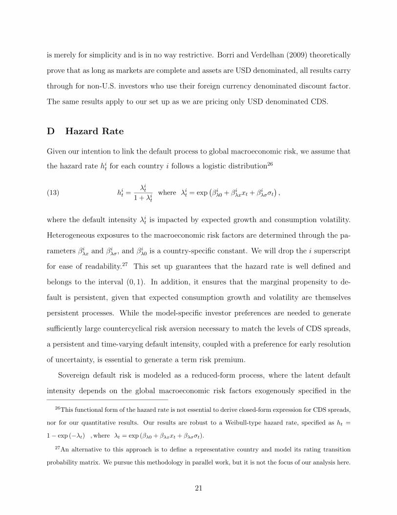
D Hazard Rate

Given our intention to link the default process to global macroeconomic risk, we assume that

the hazard rate hit for each country i follows a logistic distribution26

(13) hit =λit

1 + λitwhere λit = exp

(βiλ0 + βiλxxt + βiλσσt

),

where the default intensity λit is impacted by expected growth and consumption volatility.

Heterogeneous exposures to the macroeconomic risk factors are determined through the pa-

rameters βiλx and βiλσ, and βiλ0 is a country-specific constant. We will drop the i superscript

for ease of readability.27 This set up guarantees that the hazard rate is well defined and

belongs to the interval (0, 1). In addition, it ensures that the marginal propensity to de-

fault is persistent, given that expected consumption growth and volatility are themselves

persistent processes. While the model-specific investor preferences are needed to generate

sufficiently large countercyclical risk aversion necessary to match the levels of CDS spreads,

a persistent and time-varying default intensity, coupled with a preference for early resolution

of uncertainty, is essential to generate a term risk premium.

Sovereign default risk is modeled as a reduced-form process, where the latent default

intensity depends on the global macroeconomic risk factors exogenously specified in the

26This functional form of the hazard rate is not essential to derive closed-form expression for CDS spreads,

nor for our quantitative results. Our results are robust to a Weibull-type hazard rate, specified as ht =

1− exp (−λt) ,where λt = exp (βλ0 + βλxxt + βλσσt).

27An alternative to this approach is to define a representative country and model its rating transition

probability matrix. We pursue this methodology in parallel work, but it is not the focus of our analysis here.

21

endowment economy. This is similar in spirit to models that link the default intensity to

observable covariates, such as in Duffie, Saita, and Wang (2007) for default prediction and

in Doshi, Ericsson, Jacobs, and Turnbull (2013) to model the dynamics of CDS spreads. We

choose to embed a reduced-form credit risk model into an equilibrium set up for two reasons.

First, a CDS payout is triggered through a credit event. Longstaff, Pan, Pedersen, and

Singleton (2010) point out that Bankruptcy does not figure among the spectrum of credit

events for sovereign contracts. This is due to the nonexistence of a formal international

bankruptcy court for sovereign borrowers. As we focus on the pricing of CDS spreads prior

to default, we are less interested in the default decision as such, but rather in sovereign

distress risk (abstracting from the ”jump-at-default” risk in the literature).28 Our set up

thus differs from the endogenous default literature starting with Eaton and Gersovitz (1981),

which typically imposes exogenous default costs, which are also necessary to justify optimal

default decisions in bad states (Arellano (2008)). Recent work by Mendoza and Yue (2012)

provides a foundation to justify these exogenous default costs and highlights the stylized

fact of countercyclicality in credit spreads (and thus default probabilities) in a business cycle

model with endogenous default.

Second, a government’s default decision is mostly strategic. Modeling an explicit default

threshold in a structural default risk model for a sovereign requires therefore additional

assumptions (such as ad-hoc exogenous default costs, for instance). Structural default models

for corporate default have successfully been integrated into equilibrium models by Chen,

Collin-Dufresne, and Goldstein (2009), Chen (2010) and Bhamra, Kuehn, and Strebulaev

(2010). The success of these models relies crucially on the ability to generate countercyclical

default probabilities. This property is obtained in our reduced-form framework if the default

intensity increases when expected growth is low and/or macroeconomic uncertainty is high.

This is guaranteed as long as βλx and βλσ are non-positive and non-negative respectively.

We emphasize that our goal is to show how a simple equilibrium model with only two

28For the rest of the paper, we will refer more generally to the term default risk.

22

macroeconomic state variables can rationalize several stylized facts of the sovereign CDS mar-

ket. We are aware that our specification implies that heterogeneity in the level of spreads

arises only because of differential sensitivity to aggregate risk. While idiosyncratic shocks

may play no role in CDS returns, they may be important for the variation in spread levels.29

We therefore derive solutions where the hazard rate contains additional country-specific

shocks. The results improve only marginally, but the number of states increases to eight,

even if we allow only for two states of the idiosyncratic Markov chain. This renders the inter-

pretation of the state-dependent results cumbersome. We therefore focus on the aggregate

risk factors only and provide the additional formulas and results in the internet appendix.

Using our pricing framework and specification of the default process, we derive in internet

appendix section (A-II.B) the conditional and unconditional cumulative default probabilities

over a (T − t)-year horizon

Probt (t < τ ≤ T | τ > t) = 1−(

Ψ>T−tζt

)(14)

Prob (t < τ ≤ T | τ > t) = 1−(

Ψ>T−tΠ),

where the maturity-dependent vector sequence{

Ψj

}satisfies the internet appendix recursion

(A-12) with initial condition Ψ0 = e, where e is the vector with all components equal to

one, and where Π denotes the vector of unconditional state probabilities. We complement

the historical cumulative default probabilities with closed-form solutions of the cumulative

default rate under the risk-neutral (Q) measure in internet appendix section (A-II.C).

E Credit Default Swap Spread

Markov chains are crucial for deriving analytical solutions for CDS spreads and their mo-

ments. We develop equation (6) in appendix (A-II.D) to characterize a K- period CDS

(15) CDSt (K) = ζ>t λs (K) ,

29We thank an anonymous referee for pointing this out.

23

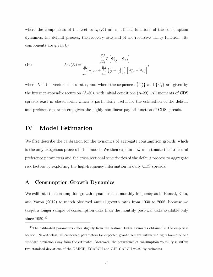
where the components of the vectors λs (K) are non-linear functions of the consumption

dynamics, the default process, the recovery rate and of the recursive utility function. Its

components are given by

(16) λi,s (K) =

KJ∑j=1

L[Ψ∗i,j −Ψi,j

]K∑k=1

Ψi,kJ +KJ∑j=1

(jJ −

⌊jJ

⌋) [Ψ∗i,j −Ψi,j

] ,

where L is the vector of loss rates, and where the sequences{

Ψ∗j}

and {Ψj} are given by

the internet appendix recursion (A-30), with initial conditions (A-29). All moments of CDS

spreads exist in closed form, which is particularly useful for the estimation of the default

and preference parameters, given the highly non-linear pay-off function of CDS spreads.

IV Model Estimation

We first describe the calibration for the dynamics of aggregate consumption growth, which

is the only exogenous process in the model. We then explain how we estimate the structural

preference parameters and the cross-sectional sensitivities of the default process to aggregate

risk factors by exploiting the high-frequency information in daily CDS spreads.

A Consumption Growth Dynamics

We calibrate the consumption growth dynamics at a monthly frequency as in Bansal, Kiku,

and Yaron (2012) to match observed annual growth rates from 1930 to 2008, because we

target a longer sample of consumption data than the monthly post-war data available only

since 1959.30

30The calibrated parameters differ slightly from the Kalman Filter estimates obtained in the empirical

section. Nevertheless, all calibrated parameters for expected growth remain within the tight bound of one

standard deviation away from the estimates. Moreover, the persistence of consumption volatility is within

two standard deviations of the GARCH, EGARCH and GJR-GARCH volatility estimates.

24

The mean expected consumption growth µx is 0.0015 with a sensitivity to long-run risk

shocks νx set to 0.038. These shocks are persistent with a value φx equal to 0.975. Con-

sumption volatility has a mean√µσ of 0.0072, a persistence φσ of 0.999 and a sensitivity to

shocks νσ of 2.80×10−6. As we want to exploit the rich information in the daily dynamics of

CDS spreads to estimate the structural default and preference parameters, we choose to map

the monthly calibrated values into a daily frequency, assuming twenty-two trading days in a

month. More specifically, we translate the monthly dynamics of consumption growth into a

daily system such that the time-averaged first and second moments of annual consumption

growth are preserved in population. For the purpose of illustration, a value of µx = 0.0015

at a monthly decision interval for the mean consumption growth corresponds to a value at

a daily decision interval equal to µdailyx = ∆µx, where ∆ = 1/22. Similarly, a value of φx =

0.975 for the persistence of the predictable component of consumption growth is translated

into a daily value equal to φdailyx = φ∆x (see Table 8 for further details).

The mapping from the continuous daily endowment process into a discrete Markov-

switching model follows the procedure described in Bonomo, Garcia, Meddahi, and Tedongap

(2011). Calibration results for the consumption growth dynamics are reported in Panel A

of Table 8, where we obtain values for all four states of nature defined by the combinations

of low (indexed by the letter L) and high (indexed by the letter H) conditional means and

variances of consumption growth. Panel B reports annualized (time-averaged) descriptive

statistics for aggregate consumption growth, which are compared against the observed values.

The mean, volatility and persistence for consumption growth of 1.8%, 2.53% and 0.46 are

consistent with the estimates of 1.92%, 2.12% and 0.46 found in the data.

B Estimation of Preference and Default Parameters

We exploit the high-frequency information in daily sovereign CDS spreads to estimate the

preference parameters as well as the cross-sectional sensitivities of the default process to the

two systematic risk factors via the Generalized Method of Moments (GMM). The weighting

25

matrix is the inverse of the diagonal of the spectral density matrix, and the moments are the

expectations of CDS spreads and their squares. We thus have 72 moments for 36 spread series

(6 maturities for each rating category) to estimate in total 21 parameters, i.e. 3 preference

parameters and 3 default parameters for each of the 6 rating groups.31 The recovery rate

is fixed at 25%, which is the standard recovery rate for sovereigns and also consistent with

Pan and Singleton (2008) and Longstaff, Pan, Pedersen, and Singleton (2010).

Estimation results with Newey-West standard errors are reported in Table 9. We fix

the subjective discount factor δ at a monthly frequency at 0.9989 and estimate the other

preference parameters. All coefficients turn out to be statistically significant at the 1%

level. Using spread levels (changes) for the estimation, we obtain a coefficient of relative risk

aversion γ of 8.2692 (7.1713). This is significantly less than the value of 20.90 estimated in

Bansal and Shaliastovich (2013), who estimate a value of 1.81 for the EIS ψ at a quarterly

model frequency. Part of the discrepancy could be due to a different decision interval, as

time-aggregation can lead to higher estimates of risk aversion. We estimate a value of the

EIS equal to 1.5774 (1.5953). The daily information in CDS spreads provides additional

support for a value of the EIS above 1 and preference for early resolution of uncertainty.

Regarding the default parameters, all signs of the coefficients are consistent with economic

intuition and imply countercyclical default probabilities.32 This feature is essential for asset

pricing implications as emphasized in Bhamra, Kuehn, and Strebulaev (2010), among others,

and helps us generate countercyclical credit spreads. Negative values for βλx suggest that a

rise in expected consumption growth lowers the marginal propensity to default. Moreover,

positive values for βλσ indicate that in times of high macroeconomic uncertainty, sovereign

debt becomes riskier and the likelihood of default increases. Thus, asset markets dislike

macroeconomic uncertainty (Bansal, Khatchatrian, and Yaron (2005)). Also, the average

default intensity is inversely related to credit-worthiness, that is the constant coefficient βλ0

31A detailed description of the estimation steps is provided in internet appendix section (A-II.E).

32Default parameter estimates using spread changes are available upon request.

26

increases from negative 15.37 to negative 9.15 for the AAA and B rating category respectively.

Furthermore, highly rated countries are more sensitive to macroeconomic uncertainty and

the pattern is monotonically decreasing, while there is no clear pattern for the sensitivity

to expected consumption growth. The last panel reports the J-statistic for the test of

overidentifying restrictions and the corresponding p-value. The model is not rejected at the

1% significance level.

V Asset Pricing Implications and Discussion

We first study the model implications for unconditional CDS moments and default proba-

bilities. Then, we investigate asset pricing results for the conditional CDS term structure.

A more detailed analysis of the hazard rate is followed by an extension of the model to

preferences that incorporate generalized disappointment aversion.

A Unconditional CDS Moments

All results for the unconditional moments of the CDS term structure are summarized in

Table 10 in the left panel. We evaluate the outcome against empirical moments in the data

reported in the right panel based on the root mean squared error (RMSE)

(17) RMSE =

√√√√ 1

K

K∑j=1

(xj − xj)2,

where K represents the CDS contract maturity, xj is the unconditional model-implied mo-

ment and xj refers to the empirical counterpart.

The model does a particularly good job in reproducing the unconditional mean, standard

deviation, skewness and first-order autocorrelation coefficients of the CDS term structure.

We generate consistently a mean upward sloping term structure for all rating categories,

in line with the data. This is consistent with the finding of persistent upward sloping term

27

structures for Mexico, Turkey and Korea reported by Pan and Singleton (2008).33 RMSEs for

the term structure of spreads are approximately 1 basis point for investment grade reference

entities, and range from 4 to 14 basis points for high-yield categories. To give an example, for

single A rated countries, the one-year (ten-year) spread is 37 (73) basis points against 35 (71)

in the data. We also fit the upward sloping term structure of volatility for groups AAA to A,

and the downward sloping volatility pattern of groups BBB to B. RMSEs range from 1 to 2

basis points for investment-grade countries, and are less than 12 basis points for high-yield

countries. Only for the B group, the RMSE is 27 basis points, implying an average error

of roughly 10% for the 5-year B volatility. In addition, the model is highly satisfactory in

reproducing the right-skewed distribution of CDS spreads and the first-order autocorrelation

coefficients of the observed spreads, which are highly persistent. While the model generates

excessive leptokurtic distributions at short maturity contracts, it reproduces the pattern

of decreasing fat tails with asset horizon and converges to the observed results at longer

maturities. We also note that the average level of spreads is higher for less-creditworthy

countries, which is consistent with the monotonic pattern in the coefficient estimates of βλ0.

In our model, time-varying global macroeconomic risk feeds into the default process.

Negative shocks to expected consumption growth and macroeconomic uncertainty are per-

sistent and create uncertainty about future default rates, which is priced. In addition to a

level risk premium, preference for early resolution of uncertainty helps to generate a term

premium, which rises with the asset horizon. In sum, with only two macroeconomic state

variables, we are able to match closely the term structure of spreads, volatility, skewness and

kurtosis, as well as the persistence of CDS spreads across 6 broad rating categories.

Before analyzing the conditional asset pricing implications and default probabilities, we

highlight that, given the calibrated endowment dynamics and estimated preference param-

eters based on sovereign CDS spreads, we remain consistent with the stock market. The

33Every country in our sample has an upward sloping term structure on average. Because of space

limitations, we have only reported summary statistics for the aggregated series in Table 2.

28

model generates a sizable equity premium of 5.52%, equity volatility of 17.48%, a risk-free

rate of 1.01% with a volatility of 0.80% (see Table 8). Thus, we provide a joint framework to

price stocks and CDS. A strong overlap in the stochastic discount factor for pricing both the

U.S. equity market and the global sovereign CDS market suggests that both are integrated

and reflects previous evidence of information flow between the two asset markets.34

B Default Probabilities

Model-results for cumulative default probabilities under the physical and risk-neutral mea-

sure, as well as their ratios, are reported in Table 11. We benchmark the model outcomes

against the historical sovereign foreign-currency cumulative average default rates reported

by Standard&Poor’s over the time period 1975 to 2009.35 Inspection of these numbers war-

rants several explanations at the outset of our discussion. Both physical and risk-neutral

default probabilities are unobserved and a proper comparison is thus close to impossible. In

particular, no country rated A or higher has defaulted within the last 40 years.36 Although

arguably very small, the default probability of a AAA rated country is unlikely zero. This

is particularly true for the CDS market, where a technical default could trigger a payout.

Therefore, we use cumulative historical default probabilities from the cash market as a first

best benchmark for comparison, but we remain critical about their use.

Given the low RMSEs, the model-implied default probabilities for CDS under the phys-

ical measure are close to their observed counterparts from the cash market. The lowest and

highest RMSEs are 0.97% and 11.11% for AAA and B rated countries respectively. Cumula-

tive default probabilities line up cross-sectionally, with the 5-year default probability ranging

from 0.79% to 22.60% for the AAA and B rated entities. Moreover, cumulative default prob-

34See Acharya and Johnson (2007) among others.

35The results benchmarked against the cumulative default rates reported by Moody’s are very similar.

36While no A rated country had an outright default, countries may be downgraded prior to default. We

study rating migrations in parallel work.

29

abilities rise with the asset horizon, which is consistent with increasing cumulative default

probabilities over time. Results are slightly better at longer than at shorter horizons.

The ratios of risk-neutral to physical default probabilities are monotonically increasing

with maturity, reflecting the term premium required for selling CDS insurance. Similar

for the physical default probabilities, the risk-neutral values are cross-sectionally increasing

for less credit-worthy countries. All ratios of risk-neutral to physical probabilities range

between 1.09 and 3.98, while the average is 2.15. These values are consistent with Berndt,

Jarrow, and Kang (2007), who find strongly time-varying ratios of implied risk neutral

default probabilities to Moody’s KMV Expected Default Frequencies between 1 and 3 for

short horizons, but going as high up as 10 in 2002. For corporate bonds, Driessen (2005)

and Huang and Huang (2012) who find average ratios of, respectively, 1.89 and 1.11 to 1.75.

C Conditional CDS Moments

The regime-switching set up of the model allows for a better understanding of the relationship

between macroeconomic risk factors and asset prices. In Figure 3, we report state-dependent

spreads for the four states of nature determined by expected growth and volatility of con-

sumption, as well as the unconditional moments.

We first note that, ceteris paribus, an increase in expected consumption growth shifts the

entire term structure downwards. These shifts are visible, for instance, when moving from

the solid to the dashed line, and from the dotted to the dash-dotted line. In contrast, a rise in

consumption volatility has the opposite effect on the level of spreads. Higher macroeconomic

uncertainty raises the level of spreads. This model-implied result is consistent with the

empirical regression results. More specifically, the projection of the first principal component,

extracted from the term structure of spreads across all countries, on the two macroeconomic

risk factors yields, respectively, a negative and positive loading on expected growth and

consumption volatility. In addition, we remind that the average country loadings on the first

principal component are maturity-invariant and uniformly positive across reference entities.

30

Thus if we believe that the first principal component is a level factor in the term structure

of spreads, then a negative coefficient a1 on expected growth in equation 2 implies that the

level of sovereign CDS spreads is lower in states of high conditional expected consumption

growth. Moreover, a positive coefficient on a2 implies that higher volatility of aggregate

consumption growth increases sovereign spreads. These results are economically intuitive

and consistent with a countercyclical level of spreads. We add that this relationship between

the level of spreads and the two macroeconomic risk factors is also obtained in the country

regressions reported in Table 7, where we use the actual level of spreads as the regressand.

Replicating these regressions inside the model, we find that the model-implied results in

population predict a negative and positive coefficient, respectively, on expected growth and

consumption volatility for the level of spreads.37 The theoretical R2 of 97% of that regression

compares favorably to the empirical value of 75%.

While global macroeconomic risk affects the level of spreads, this effect is asymmetric

across maturities and thereby affects the slope of spreads. Irrespectively of whether consump-

tion volatility is high or low, a positive growth outlook steepens the CDS term structure.

This is because a positive contemporaneous shock to expected consumption growth will de-

crease default probabilities, given the negative estimates of βλx. The improved likelihood

of default is particularly pronounced at shorter horizons, since at longer horizons, there is

greater uncertainty and a higher probability of negative shocks to expected growth (and

therefore higher default probabilities). Given preference for early resolution of uncertainty,

this commands a term premium, which increases the slope of the term structure. This model-

implied feature is also reflected in the positive slope coefficient a1 from the regression of the

second principal component on expected consumption growth reported in regression (2) of

Table 5, if we are to interpret the second principal component as a slope factor. It is likewise

37Observe that in the model, the Variance Risk Premium is perfectly collinear with expected consumption

growth and volatility. Comparing the model predictions for the slope coefficients and R2 to the empirical

observations when all factors are included in the specification is thus not possible.

31

consistent with the country regressions, where more than half of the regression coefficients

for the slope are positive. Columns (10) to (12) of Table 7 show that, in the model, expected

growth positively predicts the slope in population with a R2 of 75%, which squares well with

a value of 74% and a positive regression coefficient in the second factor regression.

The relationship between consumption volatility and the slope depends on the perception

of future economic conditions. If expected consumption growth is low, higher macroeco-

nomic uncertainty will decrease the slope of the term structure. However, conditional on

high expected consumption growth, the term structure steepens following a positive shock to

macroeconomic uncertainty. The positively estimated hazard rate coefficients βλσ indicate

that a rise in uncertainty increases default probabilities and therefore raises spreads. In times

of high expected growth, if the agent expects more volatility in the future, with preference

for early resolution of uncertainty, he will command a term premium because of the aversion

towards uncertainty shocks. This increases the slope. However, if expected growth is low,

a positive volatility shock pushes the marginal investor into the worst economic state and

induces a strong deterioration of conditional default probabilities. Conditional on survival,

default probabilities are expected to be lower at longer horizons and this effect dominates

over a term risk premium. Unconditionally, we expect the positive relationship between un-

certainty and the slope of spreads to dominate as in our model the unconditional probability

of being in a state of high expected consumption growth (≈89%) is larger than the proba-

bility of being in a state of low expected growth (≈11%). Indeed, this outcome is predicted

by the model-implied replication of the country regressions in columns (10) to (12) of Table

7. This explanation also rationalizes the positive regression coefficient a2 in column (2) of

Table 5 if we believe the second principal component to be a slope factor.

Figure 3 further emphasizes that the slope of the term structure inverts in times of low

expected growth and high macroeconomic uncertainty. The economic magnitude of the

inversion ranges from 9 to 93 basis points, in absolute value, for the AAA and B rating

categories respectively. Thus, an investor becomes much more risk averse in bad economic

32

times and requires higher compensation to offer protection on sovereign default. This jacks

up the price of CDS at short horizons. The possibility of reverting back to sound economic

fundamentals introduces mean reversion and spreads converge back to lower levels at longer

horizons. But as shocks are persistent, the average level remains elevated.

For the purpose of comparison, we plot in Figure 4 the historical difference between the

10 and 1-year CDS spread of four European distressed economies during the sovereign debt

crisis in the north-east corner of the figure.38 In the year prior to default, Greece was rated

B. Within our sample, the slope of its CDS term structure inverted by a maximum of 525

basis points and the average slope across reversal dates is 195 basis points. This is about

twice as large as the inverted spread curve of 93 basis points generated by the model in the

worst state. In addition, Portugal, which was rated A in 2010, had a maximum reversal

of approximately 150 basis points and an average inverted slope of 68 points, which is also

a bit more than twice the conditionally inverted slope of 26 basis points. Moreover, the

mean (highest) slope reversal for Spain, which was downgraded to AA+ in 2010, was 29

(56) basis points, which again is twice the negative slope of 14 basis points. The slope of

Italy didn’t decrease as much during our sample period, but it continued to decrease as the

sovereign debt crisis intensified. In sum, the conditional moments of our model qualitatively

match the slope reversal of distressed sovereign borrowers in states of bad macroeconomic

fundamentals. We quantitatively underestimate the inversion by about 50%.

D An Analysis of the Hazard Rate

To provide further intuition about how the effects of the systematic risk factors affect the

term structure, we plot in Figure 5 the results of our benchmark model against different

specifications of the hazard process from equation 13. The solid bullet points are the un-

conditional moments from the data and the dashed-dotted line represents the unconditional

moments when both expected consumption growth and volatility are active. With a constant

38Graphs for other rating categories than AA, A and B look very similar and are available upon request.

33

default process (dashed line), the term structure is flat. This is not surprising, as default

intensities become deterministic, and we expect no term premium. On the other hand, a

specification with only expected consumption growth (dotted line) creates a term structure,

which is way too steep, while the opposite is true, when consumption volatility is the only

risk driver. Thus, the first and second moments of aggregate macroeconomic risk have offset-

ting effects on the term structure, and a two-factor model is necessary to reproduce stylized

facts observed in the data. This compares with Pan and Singleton (2008) and Longstaff,

Pan, Pedersen, and Singleton (2010) for example, who use a one-factor model. However, the

authors argue that a one-factor model is acceptable, but that a two-factor model may be

desirable.

E An Extension to Preferences with Downside Risk Aversion

Our model is successful in matching the unconditional moments of the term structure, but

we quantitatively underestimate the inversion of the term structure in the worst economic

state. We try to improve upon this dimension by extending our benchmark scenario with

symmetric recursive preferences and a Kreps and Porteus (1978) (KP) certainty equivalent

to that of a risk averse investor with generalized disappointment averse (GDA) preferences of

Routledge and Zin (2010).39 This framework is well suited as GDA preferences endogenously

generate higher risk aversion in the worst economic state. The extended model derivations

are relegated to the external appendix. Beside the subjective discount factor δ, the coef-

ficient of relative risk aversion γ and the elasticity of intertemporal substitution ψ, GDA

preferences are characterized through two additional preference parameters. The coefficient

of disappointment aversion, α, defines the weight attributed to disappointing outcomes. A

state-contingent outcome is only disappointing if it falls below a fraction κ of the certainty

equivalent. We first discuss the estimation results, then the asset pricing implications.

Table 9 shows that the additional degree of freedom slightly improves the fit of the

39In fact, the GDA preferences of Routledge and Zin (2010) nest those of Epstein and Zin (1989).

34

model. The model is not rejected and the J-Test statistic is a bit lower than in the KP

case with a value of 14.65. A likelihood ratio test rejects the benchmark model against

the alternative with generalized disappointment averse preferences.40 Fixing the subjective

discount factor at 0.9989, we find that all coefficients are statistically significant at the 1%

level. Using spread levels (changes), we estimate a coefficient of relative risk aversion γ of

4.9081 (5.0614) and an EIS ψ equal to 1.4874 (1.2473). Similar to the benchmark case, this

implies a value for the EIS above 1 and preference for early resolution of uncertainty. The

parameter of disappointment aversion α is equal to 0.2486 (0.4819), implying that the ratio

of investor’s marginal utility of wealth for non-disappointing to disappointing outcomes is

25% (48%).41 The parameter κ, which measures the fraction of the certainty equivalent

below which disappointment kicks in, is estimated to be 0.8470 (0.9549). Estimation of the

generalized disappointment averse preference parameters using derivative pricing information

in the fixed income market is a novel result in the literature.

Table 12 illustrates that the performance of the KP and GDA scenarios are similar for

the unconditional moments of the CDS term structure. The GDA model performs slightly

better for the mean term structure, with RMSEs ranging between 0.52 and 9.60 basis points

respectively. On the other hand, the model generates comparable results for the volatility,

skewness and persistence of CDS spreads. In addition, it introduces slightly higher kurtosis

at the short end of the curve for the asset distributions.

Figure 3 further illustrates that the downside risk aversion steepens the inversion of

the term structure in states of low expected consumption growth and high macroeconomic

uncertainty. Asymmetric preferences thus improve the fit in the worst economic state if we

compare the model-implied results against the average term structure inversion of rating-

equivalent countries in distress during the sovereign debt crisis, as we do in Figure 3 for the

40For the estimation using spread changes, we also reject the KP model in favor of GDA preferences.

41A value of α equal to 0.25 maps into a loss aversion parameter of 3, a well accepted measure in the

literature for loss aversion.

35

benchmark case. An investor who cares about downside risk jacks up the price of credit

protection much more in the worst economic state. The magnitude of the slope reversal

in the bad state is consistently about twice the value obtained with symmetric preferences.

The 10 minus 1 year slope decreases from -17 basis points for AAA countries, to a minimum

of -169 basis points for the worst rating category B. We thus find that both the KP and the

GDA economies manage to match the unconditional moments of the CDS term structure

well. However, a model with downside risk performs better in capturing conditional stylized

facts because it allows for higher risk aversion in states of bad macroeconomic fundamentals.

Finally, we highlight that the high levels of CDS spreads in states of low expected con-

sumption growth and high macroeconomic uncertainty, which on average occur only 2.3% of

the time, implicitly reflect the tail risk embedded in CDS spreads. For instance, the average

1-year BBB CDS spread is 83 basis points, but there is a huge price discrepancy across

states. The “low-high” state for example has a spread of 552 basis points, but spreads for

the other three states are very low, with a maximum of 187 basis points for times of low ex-

pected growth and macroeconomic uncertainty. Conceptually, this result resembles Berndt

and Obreja (2010), who empirically show that a large fraction of European corporate CDS

returns are explained by a factor mimicking economic catastrophe risk.

VI Conclusion

We show that expected growth and consumption volatility in the U.S. contain information to

account for 75% of the variation of the first two principal components in the term structure

of CDS spreads, which we believe to be a level and slope factor. This information is not

accounted for by a battery of financial market variables such as the VIX index, the VRP,

the excess return on the U.S. stock market, the price-earnings ratio or the investment-grade

and high-yield bond spreads. While some of these variables have individually explanatory

power for the level factor, none of them can account for the variation in the slope factor.

36

To rationalize these empirical findings, we show that a simple equilibrium model with

only two state variables can account for many stylized facts of the sovereign CDS market.

We essentially embed a reduced-form credit risk model into a recursive utility framework.

Time-varying expected growth and macroeconomic uncertainty drive variation in both the

pricing kernel and the default process. Countries differ cross-sectionally by their sensitivities

to aggregate risk. Our model yields tractable closed-form solutions. Countercyclical risk

aversion and a persistent time-varying default process are necessary to match unconditional

moments up to the fourth order and persistence of the CDS term structure, as well as cumu-

lative historical default probabilities at aggregate levels. We extend the model to preferences

with generalized disappointment aversion and show that downside risk improves the fit of

observed downward sloping term structures in states of bad macroeconomic fundamentals.

To the best of our knowledge, the model is the first application of the recursive utility frame-

work to CDS spreads. We also exploit the high-frequency information in the sovereign CDS

market to estimate the preference parameters of the model. The evidence is consistent with

preference for early resolution of uncertainty and a value for the EIS above 1.

Our results emphasize global macroeconomic risk channels as a source of common vari-

ation in the levels of sovereign spreads, beyond the well-documented financial risk channel.

It will be useful to pursue this route to understand the dynamics of the term structure in

relation to both global and local risk factors, such as in Augustin (2012).

References

Acharya, V. V., and T. C. Johnson. “Insider Trading in Credit Derivatives.” Journal of

Financial Economics, 84 (2007), 110–141.

Ang, A., and F. A. Longstaff. “Systemic Sovereign Credit Risk: Lessons from the U.S. and

Europe.” Journal of Monetary Economics, 60 (2013), 493–510.

37

Arellano, C. “Default Risk and Income Fluctuations in Emerging Economies.” American

Economic Review, 98 (2008), 690–712.

Augustin, P. “The Term Structure of CDS Spreads and Sovereign Credit Risk.” Working

Paper, McGill University (2012).

Backus, D. K.; P. J. Kehoe; and F. E. Kydland. “International Real Business Cycles.”

Journal of Political Economy, 100 (1992), 745–775.

Baek, I.-M.; A. Bandopadhyaya; and C. Du. “Determinants of Market-Assessed Sovereign

Risk: Economic Fundamentals or Market Risk Appetite?” Journal of International Money

and Finance, 24 (2005), 533–548.

Bansal, R.; V. Khatchatrian; and A. Yaron. “Interpretable Asset Markets?” European Eco-

nomic Review, 49 (2005), 531–560.

Bansal, R.; D. Kiku; I. Shaliastovich; and A. Yaron. “Volatility, the Macroeconomy, and

Asset Prices.” Forthcoming, Journal of Finance (2013).

Bansal, R.; D. Kiku; and A. Yaron. “An Empirical Evaluation of the Long-Run Risks Model

for Asset Prices.” Critical Finance Review, 1 (2012), 183–221.

Bansal, R., and I. Shaliastovich. “A Long-Run Risks Explanation of Predictability Puzzles

in Bond and Currency Markets.” Review of Financial Studies, 26 (2013), 1–33.

Bansal, R., and A. Yaron. “Risks for the Long Run: A Potential Resolution of Asset Pricing

Puzzles.” Journal of Finance, 59 (2004), 1481–1509.

Benzoni, L.; P. Collin-Dufresne; R. S. Goldstein; and J. Helwege. “Modeling Credit Conta-

gion via the Updating of Fragile Beliefs.” Working Paper 2012-04, Federal Reserve Bank

of Chicago (2012).

Berndt, A.; R. A. Jarrow; and C. Kang. “Restructuring Risk in Credit Default Swaps: An

Empirical Analysis.” Stochastic Processes and their Applications, 117 (2007), 1724–1749.

38

Berndt, A., and I. Obreja. “Decomposing European CDS Returns.” Review of Finance, 14

(2010), 189–233.

Bhamra, H. S.; L.-A. Kuehn; and I. A. Strebulaev. “The Levered Equity Risk Premium and

Credit Spreads: A Unified Framework.” Review of Financial Studies, 23 (2010), 645–703.

Bollerslev, T. “Generalized autoregressive conditional heteroskedasticity.” Journal of Econo-

metrics, 31 (1986), 307 – 327.

Bonomo, M.; R. Garcia; N. Meddahi; and R. Tedongap. “Generalized Disappointment Aver-

sion, Long-run Volatility Risk, and Asset Prices.” Review of Financial Studies, 24 (2011),

82–122.

Borri, N., and A. Verdelhan. “Sovereign Risk Premia.” Working Paper 1343746, SSRN eLi-

brary (2009).

Campbell, J. Y., and J. H. Cochrane. “By Force of Habit: A Consumption-Based Explanation

of Aggregate Stock Market Behavior.” Journal of Political Economy, 107 (1999), 205–251.

Campbell, J. Y., and G. B. Taksler. “Equity Volatility and Corporate Bond Yields.” Journal

of Finance, 58 (2003), 2321–2349.

Chen, H. “Macroeconomic Conditions and the Puzzles of Credit Spreads and Capital Struc-

ture.” Journal of Finance, 65 (2010), 2171–2212.

Chen, L.; P. Collin-Dufresne; and R. S. Goldstein. “On the Relation between the Credit

Spread Puzzle and the Equity Premium Puzzle.” Review of Financial Studies, 22 (2009),

3367–3409.

Doshi, H.; J. Ericsson; K. Jacobs; and S. M. Turnbull. “Pricing Credit Default Swaps with

Observable Covariates.” Review of Financial Studies, 26 (2013), 2049–2094.

Driessen, J. “Is Default Event Risk Priced in Corporate Bonds?” The Review of Financial

Studies, 18(2005), 165–195.

39

Duffie, D. “Credit Swap Valuation.” Financial Analysts Journal, 55 (1999), 73–87.

Duffie, D.; L. Saita; and K. Wang. “Multi-period Corporate Default Prediction with Stochas-

tic Covariates.” Journal of Financial Economics, 83 (2007), 635 – 665.

Eaton, J., and M. Gersovitz. “Debt with Potential Repudiation: Theoretical and Empirical

Analysis.” Review of Economic Studies, 48 (1981), 289–309.

Epstein, L. G., and S. E. Zin. “Substitution, Risk Aversion, and the Temporal Behavior of

Consumption and Asset Returns: A Theoretical Framework.” Econometrica, 57 (1989),

937–969.

Geyer, A.; S. Kossmeier; and S. Pichler. “Measuring Systematic Risk in EMU Government

Yield Spreads.” Review of Finance, 8 (2004), 171–197.

Glosten, L. R.; R. Jagannathan; and D. E. Runkle. “On the Relation between the Expected

Value and the Volatility of the Nominal Excess Return on Stocks.” Journal of Finance,

48 (1993), 1779–1801.

Gonzalez-Rozada, M., and E. L. Yeyati. “Global Factors and Emerging Market Spreads.”

Economic Journal, 118 (2008), 1917–1936.

Hamilton, J. D. Time Series Analysis. Princeton University Press, New Jersey (1994).

Hansen, L. P. “Beliefs, Doubts and Learning: Valuing Macroeconomic Risk.” American

Economic Review, 97 (2007), 1–30.

Hansen, L. P.; J. C. Heaton; and N. Li. “Consumption Strikes Back? Measuring Long-Run

Risk.” Journal of Political Economy, 116 (2008), 260–302.

Hansen, L. P., and T. J. Sargent. “Fragile Beliefs and the Price of Uncertainty.” Quantitative

Economics, 1 (2010), 129–162.

40

Heston, S., and S. Nandi. “A Closed-form GARCH Option Valuation Model.” Review of

Financial Studies, 13 (2000), 585–625.

Huang, J.-Z., and M. Huang. “How Much of the Corporate-Treasury Yield Spread Is Due to

Credit Risk?” Review of Asset Pricing Studies, 2 (2012), 153–202.

Joslin, S.; A. Le; and K. J. Singleton. “Why Gaussian Macro-finance Term Structure Models

are (Nearly) Unconstrained Factor-VARs.” Journal of Financial Economics, 109 (2013),

604–622.

Kreps, D. M., and E. L. Porteus. “Temporal Resolution of Uncertainty and Dynamic Choice

Theory.” Econometrica, 46 (1978), 185–200.

Longstaff, F. A.; J. Pan; L. H. Pedersen; and K. J. Singleton. “How Sovereign is Sovereign

Credit Risk?” American Economic Journal: Macroeconomics, 3 (2011), 75–103.

Lustig, H.; N. Roussanov; and A. Verdelhan. “Countercyclical Currency Risk Premia.” Jour-

nal of Financial Economics, 111 (2014), 527–553.

Mendoza, E. G., and V. Z. Yue. “A General Equilibrium Model of Sovereign Default and

Business Cycles.” Quarterly Journal of Economics, 127 (2012), 889–946.

Nelson, D. B. “Conditional Heteroskedasticity in Asset Returns: A New Approach.” Econo-

metrica, 59 (1991), 347–370.

Pan, J., and K. J. Singleton. “Default and Recovery Implicit in the Term Structure of

Sovereign CDS Spreads.” Journal of Finance, 63 (2008), 2345–2384.

Reinhart, C. M., and K. S. Rogoff. “This Time is Different: A Panoramic View of Eight Cen-

turies of Financial Crises.” Working Paper 13882, National Bureau of Economic Research

(2008).

Remolona, E.; M. Scatigna; and E. Wu. “The Dynamic Pricing of Sovereign Risk in Emerging

Markets: Fundamentals and Risk Aversion.” Journal of Fixed Income, 17 (2008), 57–71.

41

Routledge, B. R., and S. E. Zin. “Generalized Disappointment Aversion and Asset Prices.”

Journal of Finance, 65 (2010), 1303–1332.

Tedongap, R. “Consumption Volatility and the Cross-Section of Stock Returns.” Forthcom-

ing, Review of Finance (2014).

Timmermann, A. “Moments of Markov Switching Models.” Journal of Econometrics, 96

(2000), 75–111.

Uribe, M., and V. Z. Yue. “Country Spreads and Emerging Countries: Who Drives Whom?”

Journal of International Economics, 69 (2006), 6–36.

Wang, H.; H. Zhou; and Y. Zhou. “Credit Default Swap Spreads and Variance Risk Premia.”

Journal of Banking & Finance, 37 (2013), 3733–3746.

Weigel, D. D., and G. Gemmill. “What Drives Credit Risk in Emerging Markets? The Roles

of Country Fundamentals and Market Co-movements.” Journal of International Money

and Finance, 25 (2006), 476 – 502.

42

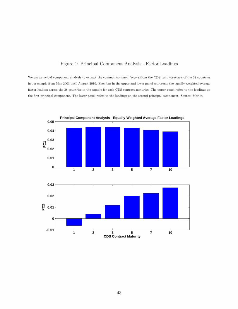
Figure 1: Principal Component Analysis - Factor Loadings

We use principal component analysis to extract the common common factors from the CDS term structure of the 38 countries

in our sample from May 2003 until August 2010. Each bar in the upper and lower panel represents the equally-weighted average

factor loading across the 38 countries in the sample for each CDS contract maturity. The upper panel refers to the loadings on

the first principal component. The lower panel refers to the loadings on the second principal component. Source: Markit.

1 2 3 5 7 100

0.01

0.02

0.03

0.04

0.05Principal Component Analysis - Equally-Weighted Average Factor Loadings

PC1

1 2 3 5 7 10-0.01

0

0.01

0.02

0.03

CDS Contract Maturity

PC2

43

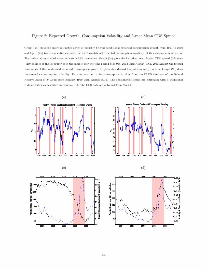
Figure 2: Expected Growth, Consumption Volatility and 5-year Mean CDS Spread

Graph (2a) plots the entire estimated series of monthly filtered conditional expected consumption growth from 1959 to 2010

and figure (2b) traces the entire estimated series of conditional expected consumption volatility. Both series are annualized for

illustration. Grey shaded areas indicate NBER recessions. Graph (2c) plots the historical mean 5-year CDS spread (left scale

- dotted line) of the 38 countries in the sample over the time period May 9th, 2003 until August 19th, 2010 against the filtered

time series of the conditional expected consumption growth (right scale - dashed line) at a monthly horizon. Graph (2d) does

the same for consumption volatility. Data for real per capita consumption is taken from the FRED database of the Federal

Reserve Bank of St.Louis from January 1959 until August 2010. The consumption series are estimated with a traditional

Kalman Filter as described in equation (1). The CDS data are obtained from Markit.

(a) (b)

(c) (d)

44

Figure 3: Model-Implied Conditional CDS Moments

Figure 3 plots the conditional and unconditional model-implied term structure of CDS Spreads for maturities 1 to 10 at the

aggregated level for the rating categories AAA to B. The recovery rate is constant and exogenously set at 25%. The preference

parameters are specified for an investor with a Kreps-Porteus (KP) certainty equivalent. The conditional states are defined

by the combinations of low (µL, σL) and high (µH , σH) expected consumption growth and volatility. The dots reflect the

unconditional moments. We also report the model-implied difference between the 10-year and 1-year CDS spreads (the Slope)

in the worst economic state µLσH . We report the model-implied results for the KP and GDA scenarios, where GDA refers to

an investor with generalized disappointment averse preferences.

Slope = CDS10y − CDS1y: State µLσH (bps)Model AAA AA A BBB BB BKP -9 -14 -26 -45 -92 -93GDA -17 -26 -47 -83 -179 -169

2 4 6 8 100

25

50

75

100

125

Spread (bp)

AAA

2 4 6 8 100

50

100

150

200AA

2 4 6 8 100

50

100

150

200

250

300

Spread (bp)

A

2 4 6 8 100

100

200

300

400

500

600BBB

2 4 6 8 100

200

400

600

800

1000

Spread (bp)

Maturity

BB

2 4 6 8 10

300

600

900

1200

1500

B

Spread (bp)

Maturity

µµµµLσσσσL

µµµµLσσσσH

µµµµHσσσσL

µµµµHσσσσH Mean

45

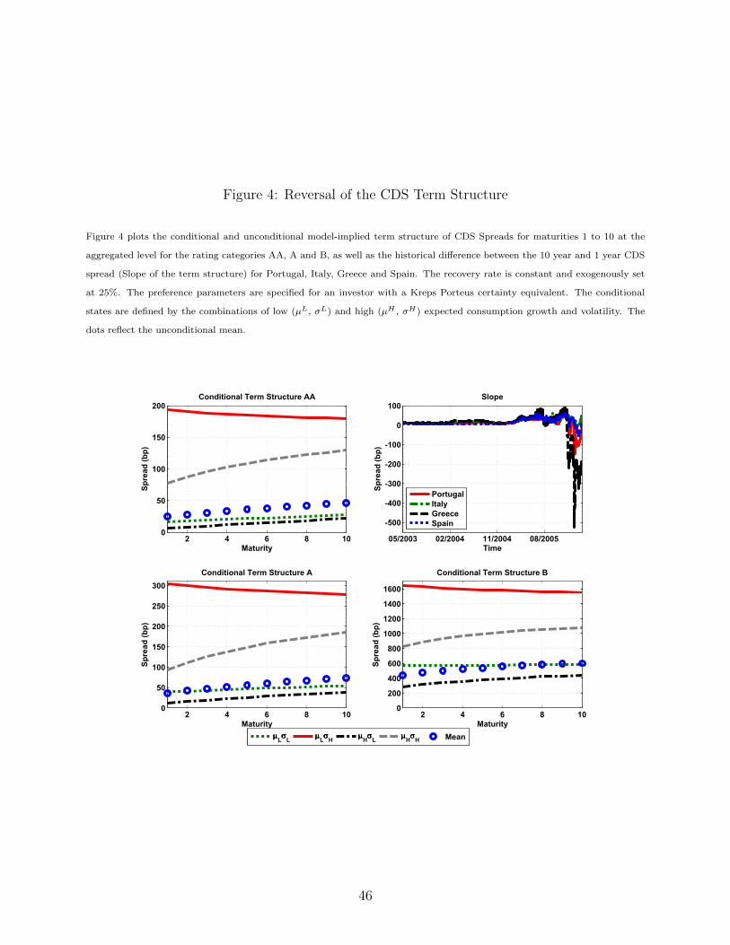
Figure 4: Reversal of the CDS Term Structure

Figure 4 plots the conditional and unconditional model-implied term structure of CDS Spreads for maturities 1 to 10 at the

aggregated level for the rating categories AA, A and B, as well as the historical difference between the 10 year and 1 year CDS

spread (Slope of the term structure) for Portugal, Italy, Greece and Spain. The recovery rate is constant and exogenously set

at 25%. The preference parameters are specified for an investor with a Kreps Porteus certainty equivalent. The conditional

states are defined by the combinations of low (µL, σL) and high (µH , σH) expected consumption growth and volatility. The

dots reflect the unconditional mean.

2 4 6 8 100

50

100

150

200Conditional Term Structure AA

Spread (bp)

Maturity05/2003 02/2004 11/2004 08/2005

-500

-400

-300

-200

-100

0

100

Time

Spread (bp)

Slope

Portugal

Italy

Greece

Spain

2 4 6 8 100

50

100

150

200

250

300

Spread (bp)

Maturity

Conditional Term Structure A

2 4 6 8 100

200

400

600

800

1000

1200

1400

1600

Conditional Term Structure B

Spread (bp)

Maturity

µµµµLσσσσL

µµµµLσσσσH

µµµµHσσσσL

µµµµHσσσσH Mean

46

Figure 5: Hazard Rate Analysis

Figure 5 plots the unconditional observed and model-implied term structure of CDS Spreads for maturities 1 to 10 at the

aggregated level for the rating categories AAA-B for various specifications of the hazard rate ht = λt/ (1 + λt), where λt =

exp (βλ0 + βλxxt + βλσσt). The dash-dotted line represents the results using the benchmark specification of the hazard rate,

the dashed line denotes the results using a constant hazard rate, whereas the dotted and solid lines feature the results for a

default process specification with only expected consumption growth or macroeconomic uncertainty respectively. The empirical

observations in the data are represented with the solid bullet points. The recovery rate is constant and exogenously set at 25%.

The preference parameters are specified for an investor with Kreps Porteus preferences.

2 4 6 8 1010

15

20

25

30

35

Spread (bp)

AAA

2 4 6 8 1020

30

40

50

60AA

2 4 6 8 1030

40

50

60

70

80

Spread (bp)

A

2 4 6 8 1070

90

110

130

150

170

BBB

2 4 6 8 10100

150

200

250

300

Spread (bp)

Maturity

BB

2 4 6 8 10400

450

500

550

600

650B

Spread (bp)

Maturity

lnλλλλt=ββββ

λλλλ 0+ββββ

λλλλ σσσσ σσσσ

tlnλλλλ

t=ββββ

λλλλ 0+ββββ

λλλλ x x

tlnλλλλ

t=ββββ

λλλλ 0+ββββ

λλλλ x x

t+ββββ

λλλλ σσσσ σσσσ

tlnλλλλ

t=ββββ

λλλλ 0 Data

47

Table 1: Country List

Table 1 presents the list of 38 countries in the sample and the corresponding geographical region. We map a country’s rating

into a numerical scheme ranging from 1 (AAA) to 21 (C). For the analysis, countries are grouped into 6 major rating buckets

(AAA, AA, A, BBB, BB, B), keeping track of rating changes over time. The third column indicates the Standard&Poor’s

Rating in 2010. The fourth column indicates the average historical rating as traced back by Fitch Ratings over the sample

period, that is from May 9th, 2003 until August 19th, 2010. The equally weighted historical average of the numerical rating is

rounded to the nearest integer to obtain the average final rating. The last two columns indicate the average number of countries

in each rating group.

Country Region S&P Rating (’10) Average Rating Classification Average # entitiesAustria Europe AAA AAA

AAA 4France Europe AAA AAAGermany Europe AAA AAASpain Europe AA AAABelgium Europe AA+ AA+

AA 6

Italy Europe A+ AA-Japan Asia AA AAPortugal Europe A- AAQatar Middle East AA AASlovenia E.Europe AA AA-Chile Lat.Amer A+ A-

A 9

China Asia A+ ACzech Republic E.Europe A AGreece Europe BB+ AIsrael Middle East A A-Korea (Republic of) Asia A A+Lithuania E.Europe BBB A-Malaysia Asia A- A-Slovakia E.Eur A+ ABulgaria E.Eur BBB BBB-

BBB 11

Croatia E.Europe BBB BBB-Hungary E.Europe BBB- BBB+Mexico Lat.Amer BBB BBB+Morocco Africa BBB- BBB-Panama Lat.Amer BBB- BBB-Poland E.Europe A- BBB+Romania E.Europe BB+ BBB-Russian Federation E.Europe BBB BBB+South Africa Africa BBB+ BBB+Thailand Asia BBB+ BBB+Brazil Lat.Amer BBB- BB

BB 6

Colombia Lat.Amer BB+ BBEgypt Africa BB+ BB+Peru Lat.Amer BBB- BB+Philippines Asia BB- BBTurkey Middle East BB BB-Lebanon Middle East B B-

B 2Venezuela Lat.Amer BB- B+

48

Tab

le2:

Sum

mar

ySta

tist

ics

Tab

le2

rep

ort

ssu

mm

ary

stati

stic

sfo

rth

eC

DS

term

stru

ctu

reof

38

sover

eign

cou

ntr

ies

over

the

sam

ple

per

iod

May

9,

2003

unti

lA

ugu

st19,

2010.

All

CD

Ssp

read

sare

mid

com

posi

tequ

ote

san

dU

SD

den

om

inate

d.

Cou

ntr

ies

are

aggre

gate

db

ase

don

6m

ajo

rra

tin

gca

tegori

esra

ngin

gfr

om

AA

Ato

B.

At

each

date

,all

ob

serv

ati

on

sw

ith

ina

giv

en

rati

ng

cate

gory

are

aggre

gate

dby

takin

gth

eeq

ually-w

eighte

daver

age

CD

Ssp

read

.F

or

the

6aggre

gate

dsp

read

seri

es,

the

tab

lere

port

sth

em

ean

,m

edia

n,

stan

dard

dev

iati

on

,

min

imu

m,

maxim

um

and

the

firs

t-ord

erau

toco

rrel

ati

on

coeffi

cien

t(A

C1).

Sou

rce:

Mark

it.

AAA

1y

2y

3y

5y

7y

10y

AA

1y

2y

3y

5y

7y

10y

Mean

14

16

18

22

23

25

24

28

31

38

41

45

Median

22

34

57

57

10

14

19

24

Sta

nd.d

ev.

23

25

27

31

31

31

38

40

42

45

45

44

Min

imum

01

12

23

12

35

68

Maxim

um

128

135

140

153

153

152

170

183

194

207

209

206

AC1

0.9

930

0.9

944

0.9

960

0.9

970

0.9

970

0.9

971

0.9

956

0.9

961

0.9

965

0.9

968

0.9

968

0.9

967

A1y

2y

3y

5y

7y

10y

BBB

1y

2y

3y

5y

7y

10y

Mean

35

42

48

60

65

71

79

95

108

130

141

152

Median

14

19

24

34

41

49

29

47

66

93

110

127

Sta

nd.d

ev.

51

55

58

63

62

61

106

108

107

104

101

97

Min

imum

46

710

13

17

11

15

20

30

37

46

Maxim

um

281

294

325

351

362

370

540

568

586

608

617

628

AC1

0.9

973

0.9

974

0.9

974

0.9

978

0.9

976

0.9

976

0.9

973

0.9

973

0.9

971

0.9

969

0.9

969

0.9

967

BB

1y

2y

3y

5y

7y

10y

B1y

2y

3y

5y

7y

10y

Mean

129

168

202

255

281

303

416

472

510

558

572

593

Median

91

143

182

244

274

294

346

399

440

489

516

540

Sta

nd.d

ev.

141

138

133

127

122

118

320

312

302

287

265

248

Min

imum

27

44

60

97

122

146

75

135

165

202

234

275

Maxim

um

1056

1077

1075

1063

1061

1065

2039

1984

1941

1881

1828

1800

AC1

0.9

954

0.9

951

0.9

948

0.9

943

0.9

939

0.9

937

0.9

931

0.9

933

0.9

933

0.9

934

0.9

930

0.9

924

49

Table 3: Principal Component Analysis

Table 3 reports the variation in CDS spreads explained by the first 6 factors PC1 to PC6 of the principal component analysis.

The row All refers to the pooled data, where all six maturities for all 38 countries are taken together. Subsequent columns

indicate results for the subsamples, taken by contract maturity (1y to 10y) each at a time. Source: Markit.

PC1 PC2 PC3 PC4 PC5 PC6All 77.8158 91.0749 94.7448 96.3491 97.5028 98.23781y 85.9812 92.8245 95.7170 97.1810 98.2461 99.05402y 83.0337 91.6612 95.5640 97.1889 98.2693 98.92293y 79.7215 91.7345 95.5324 97.1032 98.1849 98.82075y 75.1912 92.0572 95.2786 96.7295 97.9724 98.70117y 72.8903 91.5746 94.8203 96.2861 97.4767 98.577910y 70.4393 91.6796 94.6215 96.2402 97.5720 98.4832

50

Table 4: Kalman Filter Estimates

Table 4 reports the Kalman Filter estimates for the parameters of the conditional expectation of consumption growth and

conditional consumption volatility for the system of equations

gt+1 = xt + σtεg,t+1

xt+1 = (1− φx)µx + φxxt + νxσtεx,t+1

σ2t+1 = (1− φσ)µσ + φσσ

2t + νσεσ,t+1,

where gt, xt and σt reflect the dynamics for, respectively, aggregate consumption growth, its conditional mean and volatility,

and all error terms are standard normal. In addition to the short-run consumption shocks εg,t+1, consumption growth is fed

with long-run shocks εx,t+1, whose persistence is defined through the parameter φx. The unconditional mean growth-rate

is given by µx and νx denotes the sensitivity of expected growth to long-run shocks. The parameters φσ and νσ define the

persistence of and sensitivity to shocks εσ,t+1 to macroeconomic uncertainty, which is fluctuating around its long-run mean µσ .

Macroeconomic uncertainty is defined as a GARCH-like stochastic volatility process that has been used in Heston and Nandi

(2000), henceforth HN. Panel A reports the results for this base specification. Standard errors are given in parentheses. Panel

B reports the estimated coefficients and standard errors in parentheses for alternative volatility specifications: the GARCH(1,1)

model of Bollerslev (1986), the EGARCH model of Nelson (1991) and the GJR GARCH model of Glosten, Jagannathan, and

Runkle (1993), which have the following dynamics:

GARCH(1, 1) : σ2t+1 = (1− φσ)µσ + φσσ

2t + νσσ

2t

(ε2c,t+1 − 1

)EGARCH : lnσ2

t+1 = (1− φσ) lnµσ + φσ lnσ2t + νσ

(|εc,t+1| −

√2/π

)+ λσεc,t+1

GJR : σ2t+1 = (1− φσ)µσ + φσσ

2t + νσσ

2t

(ε2c,t+1 − 1

)+ λσσ

2t

(ε2c,t+1I (εc,t+1 < 0)−

1

2

),

where the additional leverage parameter λσ in the EGARCH and GJR-GARCH specifications allows for asymmetric effects of

positive and negative shocks to volatility. All coefficients are estimated using data for real per capita consumption growth from

the FRED database of the Federal Reserve Bank of St.Louis from January 1959 until August 2010.

Panel A µx φx νx µσ φσ νσ

HN0.001785 0.955642 0.058611 1.372177e-05 0.9610790 7.5528e-007

(0.000235) (0.033936) (0.028885) (1.541653e-06) (0.013410) (1.7537e-007)

Panel B µσ φσ νσ λσ

GARCH(1,1)9.0536e-06 0.97791 0.03598 –

(1.0199e-05) (0.00364) (0.00840) (–)

EGARCH1.5787e-05 0.99068 0.09589 0.02269

(4.5563e-06) (0.00460 (0.02338) (0.00969)

GJR1.3293e-05 0.98495 0.07086 −0.03128

(1.6063e-05) (0.00554) (0.01731) (0.01736)

51

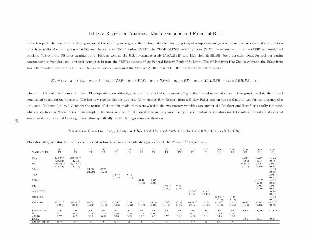
Table 5: Regression Analysis - Macroeconomic and Financial Risk

Table 5 reports the results from the regression of the monthly averages of the factors extracted from a principal component analysis onto conditional expected consumption

growth, conditional consumption volatility and the Variance Risk Premium (VRP), the CBOE S&P500 volatility index (VIX), the excess return on the CRSP value-weighted

portfolio (USret), the US price-earnings ratio (PE), as well as the U.S. investment-grade (AAA BBB) and high-yield (BBB BB) bond spreads. Data for real per capita

consumption is from January 1959 until August 2010 from the FRED database of the Federal Reserve Bank of St.Louis. The VRP is from Hao Zhou’s webpage, the USret from

Kenneth French’s website, the PE from Robert Shiller’s website, and the VIX, AAA BBB and BBB BB from the FRED H15 report.

Fi,t = a0,i + a1,i × xt|t + a2,i × σt + a3,i × V RPt + a4,i × V IXt + a5,i × USrett + a6,i × PEt + a7,i ×AAA BBBt + a8,i ×BBB BBt + εt,

where i = 1, 2 and t is the month index. The dependent variables Fi,t denote the principal components, xt|t is the filtered expected consumption growth and σt the filtered

conditional consumption volatility. The last row reports the decision rule (A = Accept, R = Reject) from a Dickey-Fuller test on the residuals to test for the presence of a

unit root. Columns (15) to (17) report the results of the probit model that tests whether the explanatory variables can predict the Reinhart and Rogoff crisis tally indicator,

which is available for 29 countries in our sample. The crisis tally is a count indicator accounting for currency crises, inflation crises, stock market crashes, domestic and external

sovereign debt crises, and banking crises. More specifically, we fit the regression specification.

Pr (Crisis = 1) = Φ(a0 + a1xt|t + a2σt + a3V RPt + a4V IXt + a5USrett + a6PEt + a7BBB AAAt + a8BB BBBt

).

Block-bootstrapped standard errors are reported in brackets. ∗∗ and ∗ indicate significance at the 1% and 5% respectively.

(1) (2) (3) (4) (5) (6) (7) (8) (9) (10) (11) (12) (13) (14) (15) (16) (17)VARIABLES F1 F2 F1 F2 F1 F2 F1 F2 F1 F2 F1 F2 F1 F2 CI CI CI

xt|t -128.16** 236.66** -0.22** -0.22** -0.22

(38.92) (22.10) (0.06) (0.07) (0.15)σt 454.81** 293.54** 0.45** 0.42* 0.99**

(77.58) (34.70) (0.17) (0.18) (0.37)VRP 23.68 -2.28 -0.01

(22.79) (5.25) (0.00)VIX 1.44** -0.15 0.04**

(0.37) (0.11) (0.01)USret -0.46 0.07 -0.01** -0.02

(0.91) (0.20) (0.00) (0.01)PE -0.04** 0.01* -0.00 0.04**

(0.00) (0.00) (0.00) (0.01)AAA BBB 17.80** -1.80 0.04

(1.71) (1.14) (0.14)BBB BB 16.84** -1.45 -0.11

(2.05) (1.18) (0.13)Constant -1.28** -0.77** -0.04 0.00 -0.30** 0.03 0.00 -0.00 1.03** -0.16* -0.25** 0.03 -0.30** 0.03 -0.59 -0.50 -3.58**

(0.20) (0.09) (0.04) (0.01) (0.06) (0.03) (0.03) (0.01) (0.12) (0.07) (0.02) (0.02) (0.03) (0.02) (0.42) (0.48) (0.76)

Observations 88 88 88 88 88 88 88 88 88 88 88 88 88 88 18,096 18,096 11,830R2 0.76 0.74 0.13 0.01 0.56 0.04 0.01 0.00 0.78 0.10 0.83 0.05 0.76 0.03adj.R2 0.75 0.74 0.12 -0.00 0.55 0.02 0.00 -0.01 0.78 0.09 0.82 0.04 0.76 0.02ps.R2 0.01 0.01 0.07Dickey-Fuller R** R** R A R** A A A R A R** A R** A

52

Table 6: Regression Analysis - Macroeconomic and Financial Risk

Table 6 reports the results from the regression of the factors extracted from a principal component analysis onto conditional expected consumption growth, conditional

consumption volatility and the Variance Risk Premium (VRP), the CBOE S&P500 volatility index (VIX), the excess return on the CRSP value-weighted portfolio (USret), the

US price-earnings ratio (PE), as well as the U.S. investment-grade (AAA BBB) and high-yield (BBB BB) bond spreads. Factor scores are first averaged at the end of each

month and then projected onto the explanatory variables. Data for real per capita consumption is taken from the FRED database of the Federal Reserve Bank of St.Louis from

January 1959 until August 2010. The data for the VRP is taken from Hao Zhou’s webpage, for the USret on Kenneth French’s website, the PE from Robert Shiller’s website,

and the VIX, AAA BBB and BBB BB from the FRED H15 report. Block-bootstrapped standard errors are reported in brackets. ∗∗ and ∗ indicate significance at the 1% and

5% respectively.

Fi,t = a0,i + a1,i × xt|t + a2,i × σt + a3,i × V RPt + a4,i × V IXt + a5,i × USrett + a6,i × PEt + a7,i ×AAA BBBt + a8,i ×BBB BBt + εt,

where i = 1, 2, 3 and t is the month index. The dependent variables Fi,t denote the principal components, xt|t is the filtered expected consumption growth and σt the filtered

conditional consumption volatility. The last row reports the decision rule (A = Accept, R = Reject) from a Dickey-Fuller test on the residuals to test for the presence of a unit

root.

(1) (2) (3) (4) (5) (6) (7) (8) (9) (10) (11) (12) (13) (14)VARIABLES F1 F2 F1 F2 F1 F2 F1 F2 F1 F2 F1 F2 F1 F2

xt|t -120.99* 239.89** -69.26 248.26** -118.87** 238.30** 164.96* 260.42** 70.69 255.43** 29.07 266.36** 136.96* 247.91**(47.79) (23.65) (62.20) (22.31) (39.96) (22.39) (69.97) (24.13) (45.69) (20.23) (40.92) (25.27) (67.02) (29.92)

σt 450.18** 291.46** 401.68** 283.08** 469.60** 296.15** 286.17** 279.87** 254.52** 274.64** 348.96** 273.55** 255.53** 280.00**(81.73) (36.66) (60.58) (38.47) (82.80) (34.99) (53.98) (39.20) (59.90) (43.13) (52.07) (33.28) (56.98) (47.37)

VRP 3.64 1.63 0.98 3.38(13.18) (1.82) (9.57) (4.79)

VIX 0.48 0.09 0.06 -0.05(0.40) (0.07) (0.33) (0.12)

USret -0.55 -0.10 0.11 0.20(0.36) (0.10) (0.33) (0.20)

PE -0.04** -0.00 -0.02 0.00(0.01) (0.00) (0.01) (0.01)

AAA BBB 14.75** 1.39 5.56 -0.76(2.73) (1.11) (4.42) (2.49)

BBB BB 11.25** 2.12* 5.94* 4.06(1.98) (0.98) (2.90) (2.28)

Constant -1.27** -0.76** -1.22** -0.76** -1.31** -0.77** 0.29 -0.64** -0.89** -0.73** -1.15** -0.74** -0.52 -0.90**(0.21) (0.09) (0.17) (0.10) (0.22) (0.09) (0.27) (0.16) (0.15) (0.11) (0.14) (0.09) (0.33) (0.22)

Observations 88 88 88 88 88 88 88 88 88 88 88 88 88 88R2 0.76 0.75 0.78 0.75 0.77 0.75 0.87 0.75 0.88 0.75 0.88 0.77 0.91 0.78adj.R2 0.75 0.74 0.77 0.74 0.77 0.74 0.86 0.74 0.87 0.74 0.88 0.76 0.90 0.76Dickey-Fuller R** R** R** R** R** R** R** R* R** R R** R* R** R*

53

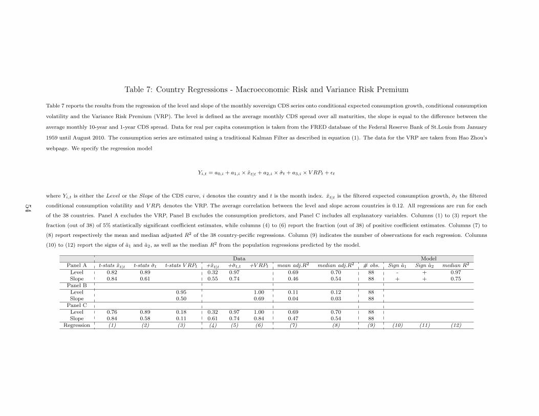
Table 7: Country Regressions - Macroeconomic Risk and Variance Risk Premium

Table 7 reports the results from the regression of the level and slope of the monthly sovereign CDS series onto conditional expected consumption growth, conditional consumption

volatility and the Variance Risk Premium (VRP). The level is defined as the average monthly CDS spread over all maturities, the slope is equal to the difference between the

average monthly 10-year and 1-year CDS spread. Data for real per capita consumption is taken from the FRED database of the Federal Reserve Bank of St.Louis from January

1959 until August 2010. The consumption series are estimated using a traditional Kalman Filter as described in equation (1). The data for the VRP are taken from Hao Zhou’s

webpage. We specify the regression model

Yi,t = a0,i + a1,i × xt|t + a2,i × σt + a3,i × V RPt + εt

where Yi,t is either the Level or the Slope of the CDS curve, i denotes the country and t is the month index. xt|t is the filtered expected consumption growth, σt the filtered

conditional consumption volatility and V RPt denotes the VRP. The average correlation between the level and slope across countries is 0.12. All regressions are run for each

of the 38 countries. Panel A excludes the VRP, Panel B excludes the consumption predictors, and Panel C includes all explanatory variables. Columns (1) to (3) report the

fraction (out of 38) of 5% statistically significant coefficient estimates, while columns (4) to (6) report the fraction (out of 38) of positive coefficient estimates. Columns (7) to

(8) report respectively the mean and median adjusted R2 of the 38 country-pecific regressions. Column (9) indicates the number of observations for each regression. Columns

(10) to (12) report the signs of a1 and a2, as well as the median R2 from the population regressions predicted by the model.

Data ModelPanel A t-stats xt|t t-stats σt t-stats V RPt +xt|t +σt,t +V RPt mean adj.R2 median adj.R2 # obs. Sign a1 Sign a2 median R2

Level 0.82 0.89 0.32 0.97 0.69 0.70 88 - + 0.97Slope 0.84 0.61 0.55 0.74 0.46 0.54 88 + + 0.75

Panel BLevel 0.95 1.00 0.11 0.12 88Slope 0.50 0.69 0.04 0.03 88

Panel CLevel 0.76 0.89 0.18 0.32 0.97 1.00 0.69 0.70 88Slope 0.84 0.58 0.11 0.61 0.74 0.84 0.47 0.54 88

Regression (1) (2) (3) (4) (5) (6) (7) (8) (9) (10) (11) (12)

54

Table 8: Parameters of the Markov-Switching Model

Consumption growth dynamics are calibrated at a monthly frequency as in Bansal, Kiku, and Yaron (2012) with µx = 0.0015,

φx = 0.975, νx = 0.038,√µσ = 0.0072, φσ = 0.999 and νσ = 2.80 × 10−6. Conditional on the information set Jt, the errors

are i.i.d. normal.

gt+1 = xt + σtεg,t+1

xt+1 = (1− φx)µx + φxxt + νxσtεx,t+1

σ2t+1 = (1− φσ)µσ + φσσ2

t + νσεσ,t+1

εg,t+1

εx,t+1

εσ,t+1

| Jt ∼ NID

0

0

0

,

1 0 0

0 1 0

0 0 1

.

To be consistent with the daily frequency of CDS spreads, we map the monthly parameters into daily values such that annual

moments of consumption growth are preserved. We use the monthly-to-daily mapping

µdailyx = ∆µx, φdailyx = φ∆x , νdailyx = νx

√√√√√(1− φ2∆x

1− φ2x

)/1 +2φx

1− φx−

2∆φx(

1− φ1/∆x

)(1− φx)2

µdailyσ = ∆µσ , φdailyσ = φ∆σ , νdailyσ = νσ

√∆

√√√√√(1− φ2∆σ

1− φ2σ

)/1 +2φσ

1− φσ−

2∆φσ(

1− φ1/∆σ

)(1− φσ)2

where we consider ∆ = 1/22, i.e. 22 trading days per month. The parameters at a daily frequency obtained from the

mapping system are µdailyx = 6.8182 × 10−5, φdailyx = 0.9988, νdailyx = 0.0019, µdailyσ = 2.3564 × 10−6, φdailyσ = 0.99995

and νdailyσ = 2.7247× 10−8. Panel A reports the parameters of the four-state daily Markov-switching model. The conditional

mean and variance of consumption growth are µg and ωg respectively. P> is the transition matrix across different regimes and

Π is the vector of unconditional probabilities of regimes. The four states are characterized by the combinations of expected

consumption growth (µ) and consumption volatility (σ), which can be high (H) and low (L). Panel B and C report the (time-

averaged) annualized model statistics for aggregate consumption growth, the risk premium and the volatility of the aggregate

stock market, the risk-free rate and its volatility, all compared against observed values. The model-implied values are reported

for both the model with the Kreps-Porteus certainty equivalent (KP) and generalized disappointment averse preferences (GDA).

The estimated values are sampled on an annual frequency from 1930 to 2008. Standard errors are reported in parentheses.

Panel A µLσL µLσH µHσL µHσHµ>g -0.00011 -0.00011 0.00009 0.00009(

ω>g)1/2

0.00094 0.00281 0.00094 0.00281

P>

µLσL 0.99897 0.00001 0.00102 0.00000µLσH 0.00004 0.99894 0.00000 0.00102µHσL 0.00013 0.00000 0.99986 0.00001µHσH 0.00000 0.00013 0.00004 0.99984

Π> 0.08600 0.02304 0.70268 0.18828Panel B Model DataE[∆g] 1.80 1.92 (0.33)σ[∆g] 2.53 2.12 (0.52)

AC1[∆g] 0.46 0.46 (0.15)Panel C Model (KP) Model (GDA) Data

E[rm − rf ] + 0.5σ2[rm] 6.38 5.52 7.84 (1.97)σ[rm] 18.48 17.48 20.16 (2.14)E[rf ] 1.22 1.01 0.86 (0.89)σ[rf ] 1.05 0.80 1.74 (0.33)

55

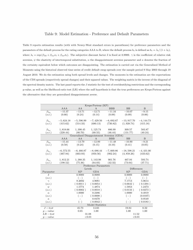
Table 9: Model Estimation - Preference and Default Parameters

Table 9 reports estimation results (with with Newey-West standard errors in parentheses) for preference parameters and the

parameters of the default process for the rating categories AAA to B, where the default process ht is defined as ht = λt/ (1 + λt),

where λt = exp (βλ0 + βλxxt + βλσσt). The subjective discount factor δ is fixed at 0.9989. γ is the coefficient of relative risk

aversion, ψ the elasticity of intertemporal substitution, α the disappointment aversion parameter and κ denotes the fraction of

the certainty equivalent below which outcomes are disappointing. The estimation is carried out via the Generalized Method of

Moments using the historical observed time series of credit default swap spreads over the sample period 9 May 2003 through 19

August 2010. We do the estimation using both spread levels and changes. The moments in the estimation are the expectations

of the CDS spreads (respectively spread changes) and their squared values. The weighting matrix is the inverse of the diagonal of

the spectral density matrix. The last panel reports the J statistic for the test of overidentifying restrictions and the corresponding

p-value, as well as the likelihood-ratio test (LR) where the null hypothesis is that the true preferences are Kreps-Porteus against

the alternative that they are generalized disappointment averse.

Kreps-Porteus (KP)AAA AA A BBB BB B

βλ0−15.37 −13.71 −12.71 −11.34 −10.07 −9.15

(s.e.) (0.66) (0.24) (0.14) (0.09) (0.09) (0.06)

βλx −5, 624.18 −5, 596.99 −7, 429.56 −6, 692.67 −13, 917.70 −4, 144.73(s.e.) (415.62) (514.33) (680.13) (730.82) (1, 928.74) (415.18)

βλσ 1, 818.66 1, 390.45 1, 125.74 886.99 309.57 583.87(s.e.) (228.44) (80.70) (68.55) (46.44) (131.77) (40.24)

Generalized Disappointment Aversion (GDA)AAA AA A BBB BB B

βλ0−15.44 −13.79 −12.89 −11.48 −10.90 −9.21

(s.e.) (0.58) (0.24) (0.15) (0.10) (0.41) (0.05)

βλx −6, 572.55 −6, 466.87 −8, 686.44 −7, 669.86 −18, 598.21 −4, 431.00(s.e.) (467.94) (663.93) (850.56) (902.24) (4, 858.26) (433.62)

βλσ 1, 812.21 1, 388.35 1, 143.98 901.76 467.94 593.74(s.e.) (198.52) (75.36) (64.03) (42.32) (73.04) (37.71)

Preference ParametersLevels Differences

Parameter KP GDA KP GDAδ 0.9989 0.9989 0.9989 0.9989

(s.e.) ( - ) ( - ) ( - ) ( - )γ 8.2692 4.9081 7.1713 5.0614

(s.e.) ( 0.0011 ) ( 0.0054 ) ( 0.0642 ) ( 0.1294 )ψ 1.5774 1.4874 1.5953 1.2473

(s.e.) ( 0.0002 ) ( 0.0018 ) ( 0.0133 ) ( 0.0273 )α 1.0000 0.2486 1.0000 0.4819

(s.e.) ( - ) ( 0.0008 ) ( - ) (0.0107)κ - 0.8470 - 0.9549

(s.e.) (- ) ( 0.0042 ) ( - ) ( 0.0183 )Model Statistics

J − test 45.73 14.65 19.84 8.32p− value 0.65 1.00 1.00 1.00LR− test 31.08 11.52p− value <0.01 <0.01

56

Table 10: Model-Implied and Observed Term Structure of CDS Spreads AAA-B

Table 10 reports observed and model-implied unconditional means, standard deviations (in basis points), skewness, kurtosis and first-order autocorrelation coefficients for CDS

spreads for maturities 1 to 10 for the rating categories AAA to B. The column labeled RMSE reports the root mean squared errors in basis points for the model fit. The

recovery rate has a constant value of 25%. Preference parameters are those of an investor with a Kreps-Porteus certainty equivalent.

MODEL DATA

AAA 1 2 3 5 7 10 RMSE 1 2 3 5 7 10Mean 14 16 17 20 23 27 1.06 14 16 18 22 23 25Volatility 25 26 27 29 30 31 1.50 23 25 27 31 31 31Skewness 2 2 2 2 2 2 0.15 2 2 2 2 2 2Kurtosis 9 7 6 5 4 3 1.12 7 7 6 5 5 4AC1 0.9997 0.9998 0.9998 0.9999 0.9999 0.9999 0.0044 0.9930 0.9944 0.9960 0.9970 0.9970 0.9971

AA 1 2 3 5 7 10 RMSE 1 2 3 5 7 10Mean 25 28 31 36 40 46 0.97 24 28 31 38 41 45Volatility 38 39 41 43 45 47 1.28 38 40 42 45 45 44Skewness 2 2 2 2 2 2 0.21 2 2 2 2 2 2Kurtosis 10 8 6 5 4 4 1.74 6 6 5 5 4 4AC1 0.9997 0.9998 0.9998 0.9999 0.9999 0.9999 0.0034 0.9956 0.9961 0.9965 0.9968 0.9968 0.9967

A 1 2 3 5 7 10 RMSE 1 2 3 5 7 10Mean 37 42 47 56 64 73 1.89 35 42 48 60 65 71Volatility 52 54 56 59 62 64 2.14 51 55 58 63 62 61Skewness 3 3 2 2 2 2 0.35 3 2 2 2 2 2Kurtosis 17 13 10 7 5 4 3.41 10 9 8 7 7 7AC1 0.9995 0.9996 0.9997 0.9998 0.9999 0.9999 0.0022 0.9973 0.9974 0.9974 0.9978 0.9976 0.9976

BBB 1 2 3 5 7 10 RMSE 1 2 3 5 7 10Mean 86 97 107 124 138 154 4.11 79 95 108 130 141 152Volatility 95 98 101 105 108 111 9.33 106 108 107 104 101 97Skewness 3 3 2 2 2 2 0.48 2 2 2 2 2 2Kurtosis 15 12 9 7 5 4 4.04 7 7 7 6 6 7AC1 0.9995 0.9996 0.9997 0.9998 0.9998 0.9999 0.0027 0.9973 0.9973 0.9971 0.9969 0.9969 0.9967

BB 1 2 3 5 7 10 RMSE 1 2 3 5 7 10Mean 136 170 199 244 278 314 7.23 129 168 202 255 281 303Volatility 159 146 136 121 111 100 11.89 141 138 133 127 122 118Skewness 3 3 3 3 3 2 0.33 3 3 3 2 2 2Kurtosis 12 12 12 12 11 10 1.85 15 14 13 11 11 10AC1 0.9989 0.9989 0.9990 0.9991 0.9992 0.9993 0.0046 0.9954 0.9951 0.9948 0.9943 0.9939 0.9937

B 1 2 3 5 7 10 RMSE 1 2 3 5 7 10Mean 442 473 498 539 569 600 14.34 416 472 510 558 572 593Volatility 282 285 287 289 289 287 27.20 320 312 302 287 265 248Skewness 2 2 2 2 2 2 0.35 2 2 2 2 2 2Kurtosis 8 7 6 5 5 4 3.33 10 9 9 8 9 9AC1 0.9997 0.9997 0.9998 0.9998 0.9998 0.9999 0.0067 0.9931 0.9933 0.9933 0.9934 0.9930 0.9924

57

Table 11: Model-Implied Term Structure of Default Probabilities AAA-B

Table 11 reports unconditional model-implied physical and risk-neutral default probabilities for maturities 1 to 10 at the

aggregated level for the rating categories AAA to B as well as their ratio. The column labeled RMSE reports the root mean

squared errors in % points for the model fit. Model results are compared against the observed Standard&Poor’s sovereign

foreign-currency cumulative average default rates over the time frame 1975 to 2009 for the physical default probabilities. The

recovery rate has a constant value of 25%.

RMSE 1y 2y 3y 4y 5y 6y 7y 8y 9y 10yPhysical Default Probabilities

AAAModel 0.97 0.16 0.32 0.48 0.63 0.79 0.94 1.10 1.25 1.40 1.55Observed − 0.00 0.00 0.00 0.00 0.00 0.00 0.00 0.00 0.00 0.00

AAModel 1.73 0.29 0.57 0.86 1.14 1.41 1.69 1.96 2.23 2.50 2.77Observed − 0.00 0.00 0.00 0.00 0.00 0.00 0.00 0.00 0.00 0.00

AModel 2.40 0.40 0.80 1.19 1.58 1.96 2.34 2.72 3.09 3.46 3.83Observed − 0.00 0.00 0.00 0.00 0.00 0.00 0.00 0.00 0.00 0.00

BBBModel 1.37 0.96 1.90 2.82 3.73 4.62 5.49 6.34 7.19 8.01 8.83Observed − 0.00 0.50 1.57 2.72 3.97 5.33 6.07 6.07 6.07 6.07

BBModel 2.02 1.25 2.45 3.61 4.74 5.84 6.92 7.99 9.03 10.06 11.08Observed − 0.74 2.36 3.70 4.70 6.36 8.24 10.34 12.72 13.63 13.63

BModel 11.11 5.19 10.00 14.49 18.68 22.60 26.28 29.75 33.00 36.08 38.98Observed − 2.13 5.03 6.71 9.32 11.67 13.54 15.85 20.06 21.87 24.57

Risk-Neutral Default ProbabilitiesAAA Model − 0.18 0.41 0.68 0.98 1.32 1.68 2.06 2.47 2.89 3.34AA Model − 0.33 0.74 1.21 1.73 2.30 2.91 3.56 4.24 4.94 5.66A Model − 0.48 1.11 1.84 2.68 3.59 4.56 5.58 6.65 7.75 8.87BBB Model − 1.13 2.52 4.10 5.84 7.69 9.62 11.60 13.62 15.65 17.69BB Model − 1.78 4.35 7.46 10.95 14.67 18.50 22.39 26.25 30.05 33.76B Model − 5.65 11.59 17.58 23.47 29.15 34.56 39.66 44.44 48.88 53.01

Ratio of Risk-Neutral to Physical Default ProbabilitiesAAA Model − 1.34 1.69 2.03 2.36 2.68 2.98 3.26 3.52 3.76 3.98AA Model − 1.22 1.44 1.65 1.84 2.03 2.21 2.37 2.53 2.67 2.80A Model − 1.27 1.51 1.72 1.92 2.11 2.27 2.43 2.57 2.70 2.82BBB Model − 1.21 1.38 1.54 1.68 1.80 1.91 2.00 2.09 2.16 2.22BB Model − 1.75 2.22 2.53 2.76 2.93 3.06 3.16 3.23 3.28 3.32B Model − 1.09 1.17 1.23 1.28 1.32 1.35 1.37 1.38 1.39 1.40

58

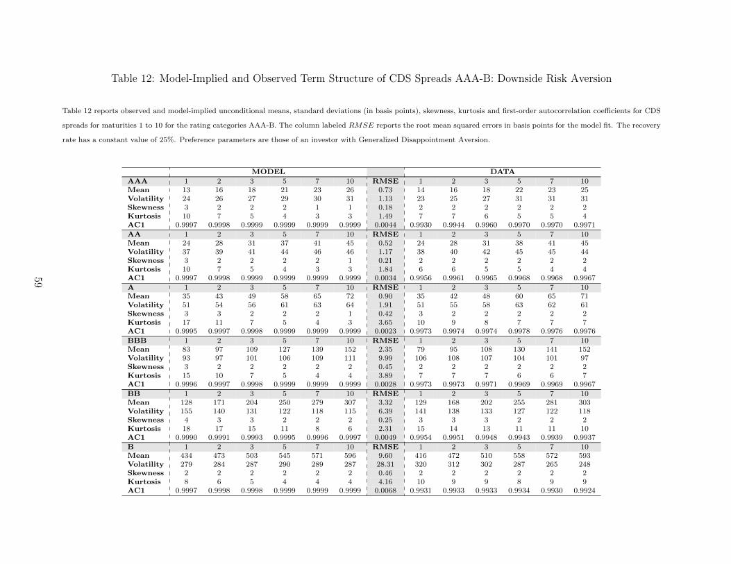
Table 12: Model-Implied and Observed Term Structure of CDS Spreads AAA-B: Downside Risk Aversion

Table 12 reports observed and model-implied unconditional means, standard deviations (in basis points), skewness, kurtosis and first-order autocorrelation coefficients for CDS

spreads for maturities 1 to 10 for the rating categories AAA-B. The column labeled RMSE reports the root mean squared errors in basis points for the model fit. The recovery

rate has a constant value of 25%. Preference parameters are those of an investor with Generalized Disappointment Aversion.

MODEL DATA

AAA 1 2 3 5 7 10 RMSE 1 2 3 5 7 10Mean 13 16 18 21 23 26 0.73 14 16 18 22 23 25Volatility 24 26 27 29 30 31 1.13 23 25 27 31 31 31Skewness 3 2 2 2 1 1 0.18 2 2 2 2 2 2Kurtosis 10 7 5 4 3 3 1.49 7 7 6 5 5 4AC1 0.9997 0.9998 0.9999 0.9999 0.9999 0.9999 0.0044 0.9930 0.9944 0.9960 0.9970 0.9970 0.9971

AA 1 2 3 5 7 10 RMSE 1 2 3 5 7 10Mean 24 28 31 37 41 45 0.52 24 28 31 38 41 45Volatility 37 39 41 44 46 46 1.17 38 40 42 45 45 44Skewness 3 2 2 2 2 1 0.21 2 2 2 2 2 2Kurtosis 10 7 5 4 3 3 1.84 6 6 5 5 4 4AC1 0.9997 0.9998 0.9999 0.9999 0.9999 0.9999 0.0034 0.9956 0.9961 0.9965 0.9968 0.9968 0.9967

A 1 2 3 5 7 10 RMSE 1 2 3 5 7 10Mean 35 43 49 58 65 72 0.90 35 42 48 60 65 71Volatility 51 54 56 61 63 64 1.91 51 55 58 63 62 61Skewness 3 3 2 2 2 1 0.42 3 2 2 2 2 2Kurtosis 17 11 7 5 4 3 3.65 10 9 8 7 7 7AC1 0.9995 0.9997 0.9998 0.9999 0.9999 0.9999 0.0023 0.9973 0.9974 0.9974 0.9978 0.9976 0.9976

BBB 1 2 3 5 7 10 RMSE 1 2 3 5 7 10Mean 83 97 109 127 139 152 2.35 79 95 108 130 141 152Volatility 93 97 101 106 109 111 9.99 106 108 107 104 101 97Skewness 3 2 2 2 2 2 0.45 2 2 2 2 2 2Kurtosis 15 10 7 5 4 4 3.89 7 7 7 6 6 7AC1 0.9996 0.9997 0.9998 0.9999 0.9999 0.9999 0.0028 0.9973 0.9973 0.9971 0.9969 0.9969 0.9967

BB 1 2 3 5 7 10 RMSE 1 2 3 5 7 10Mean 128 171 204 250 279 307 3.32 129 168 202 255 281 303Volatility 155 140 131 122 118 115 6.39 141 138 133 127 122 118Skewness 4 3 3 2 2 2 0.25 3 3 3 2 2 2Kurtosis 18 17 15 11 8 6 2.31 15 14 13 11 11 10AC1 0.9990 0.9991 0.9993 0.9995 0.9996 0.9997 0.0049 0.9954 0.9951 0.9948 0.9943 0.9939 0.9937

B 1 2 3 5 7 10 RMSE 1 2 3 5 7 10Mean 434 473 503 545 571 596 9.60 416 472 510 558 572 593Volatility 279 284 287 290 289 287 28.31 320 312 302 287 265 248Skewness 2 2 2 2 2 2 0.46 2 2 2 2 2 2Kurtosis 8 6 5 4 4 4 4.16 10 9 9 8 9 9AC1 0.9997 0.9998 0.9998 0.9999 0.9999 0.9999 0.0068 0.9931 0.9933 0.9933 0.9934 0.9930 0.9924

59