The macroeconomic effects of expenditure shocks during good and bad times

Francesco Caprioli and Sandro Momigliano*

Abstract

We study how the effects of expenditure shock on economic activity are influenced by the state of the economy on the basis of various autoregressive models and indicators of cyclical conditions. For Italy over the period 1982-2011 we find some, but not conclusive, evidence that expenditure multipliers tend to be higher in recessions than in expansions.

JEL Classification: C13, H30, H63.

Keywords: fiscal multipliers, threshold VAR, sovereign debt.

Paper presented at the Workshop “The Sovereign Debt Crisis and the Euro Area” organized by the Bank of Italy and held in Rome on February 15, 2013. The proceedings are available at:http://www.bancaditalia.it/studiricerche/convegni/atti.

* Bank of Italy, Structural Studies Department, Public Finance Division. E-mail: sandro.momigliano@bancaditalia.it. The views expressed in the paper do not necessarily reflect those of the Banca d’Italia. All errors are the responsibility of the authors.

368

1 Introduction

The large stimulus packages implemented by governments in most advanced countries to contrast the global recession that begun in mid-2008 stimulated a large debate (see Corsetti et al., 2010; Romer and Romer, 2010) and brought renewed attention to the old question of the usefulness of fiscal policy to smooth cyclical fluctuations. More recently, a similar debate stemmed from fiscal consolidation policies and focused on the size of fiscal multipliers (IMF, 2102).

The theoretical literature provides limited guidance on these issues, as the qualitative effects of fiscal policy are model-dependent (see Cogan et al., 2009); the empirical evidence is still not conclusive either, although it suggests that fiscal expansions generally boost private consumption and output.1

It has been often pointed out that the effects of fiscal policy may depend on the state of the economy (e.g., Parker, 2011; IMF, 2012), but there is still little empirical research trying to assess how the size of fiscal multipliers varies over the cycle. Indeed, most of the existing empirical literature uses linear models which, by construction, are unable to capture any dependence of fiscal multipliers on the level of aggregate demand.

In this paper we contribute to the debate by estimating for the Italian economy various threshold VARs, which allow to analyze the influence of the state of the economy on the effects of expenditure shocks. In particular, we study whether the traditional Keynesian argument of higher effectiveness of fiscal stimulus in periods characterized by slack of resources is supported by the Italian data. Similar analyses have been carried out for other countries (e.g. Canova and Pappa, 2011; De Cos et al., 2013).

Our starting point is the Structural VAR (SVAR) employed in Caprioli and Momigliano (2011). Fiscal shocks are identified using the methodology developed by Blanchard and Perotti (2002), which delivers relatively efficient estimates in small samples as recently stressed by Chahrour et al. (2010).2 The model includes two additional variables – government debt and foreign demand – with respect to the standard model found in the literature (5 variables: private GDP, inflation, interest rates, net revenue and government consumption). The inclusion of debt is important because it allows to take into account its influence on the fiscal authorities’ decisions, particularly important in the case of Italy.3 The inclusion of foreign demand is warranted by its strong influence on economic activity, Italy being a small open economy.

To take into account the state of the economy we first estimate the SVAR described above splitting the sample into “recessions” and “expansions” on the basis of the official chronology of the Italian economy published by Isco/Isae/Istat (Altissimo et al, 1999; Istat, 2011), which

————— 1 See Coenen et al. (2010). The two main empirical approaches that attempt to assess the effects of fiscal policy have specific limits.

Reliable and non-interpolated quarterly fiscal data over a sufficiently long period of time, a prerequisite for the VAR approach, exist only for a few countries. The “narrative” approach (i.e., Ramey and Shapiro, 1997, and Edelberg et al., 1999) is resource-intensive and intrinsically subjective, making it almost impossible to apply across countries.

2 Other approaches most commonly used to identify structural shocks are the sign restrictions on impulse responses (see Mountford

and Uhlig, 2002), the dummy variable one (see, e.g., Romer and Romer, 2010) and the Choleski ordering one, see, e.g., Fatás and Mihov, 2001. The literature about the effects of fiscal policy using Vector Autoregression is large and to offer a comprehensive survey goes beyond the scope of this paper. See Blanchard and Perotti (2002), Perotti (2004), Fatás and Mihov (2001), Mountford and Uhlig (2002), Giordano et al. (2008), Ramey and Shapiro (1997), Edelberg et al. (1999), and Burriel et al. (2010) among many others.

3 Other researchers have included public debt in a SVAR exercise examining fiscal multipliers. We broadly follow the methodology

of Favero and Giavazzi (2007), who add a deterministic equation linking debt dynamics to the government budget balance. Chung and Leeper (2007) employ a conceptually similar approach. Creel et al. (2005) include public debt as an additional variable. This second approach allows the analysis of the effects of direct shocks on government debt. This, however, comes at the cost of estimating a higher number of parameters than actually needed, as the government budget constraint is disregarded.

369

identifies recessions following the methodology used for the US by the National Bureau of Economic Research.

Secondly, to assess the robustness of our results to different ways of identifying recessions and also to overcome the problem arising from the limited number of observations for such regime in the official chronology we estimate an Endogenous Threshold VAR (Fazzari et al., 2012). This approach allows to endogenously identify recessions and expansions, based on an indicator of cyclical conditions. As in the previous analysis, the sample is split and two sets of parameters are estimated. We apply this method to 2 alternative indicators of cyclical conditions: the past private GDP growth and the output gap measured by the difference between the private GDP and its H.P. filter. These two indicators, commonly used in central banks, are chosen as they proxy the slack of resources in the economy.

Finally, we estimate the Smooth Transition VAR model proposed by Auerbach and Gorodnichenko (2012), which allows a gradual transition between recessions and expansion: in each quarter, the parameters of the model are a linear combination of two sets of values (corresponding to each regime), weighted by the degree of being in each regime.

The main results of this paper can be summarized as follows.

In the SVAR analysis which doesn’t take into account the state of the economy, the response of private GDP to an expenditure shock is positive, hump-shaped and highly significant for approximately two years. The median value of the expenditure multiplier is equal to 1.04 on impact and reaches its peak (1.8) after three years.

When we split the sample in “expansion” and “recession” regimes, either on the basis of the official chronology or applying the ETVAR approach to the cyclical indicators, for both regimes we obtain impulse response functions (IRFs) broadly similar to those estimated for the full sample. Under the recession regime, the response of private GDP is larger and more prompt and the cumulative multiplier is stronger on average. However, the confidence bands of the estimate are relatively large, and the difference in the median value of the multiplier across regimes is not statistically significant. This difference is instead statistically significant if we apply the ETVAR analysis to the 3-variable model (namely, private GDP, government consumption and net revenue) originally proposed in Blanchard and Perotti (2002), which is more parsimonious in terms of parameters.

Estimates are generally less precise and results are less clear-cut when we apply the STVAR model: in recessions the median value of the expenditure multiplier can be higher or lower depending on the cyclical indicator used.

In conclusion, our empirical investigation shows some weak evidence that expenditure multipliers are higher in recessions than in expansions. While this result is influenced by the limited size of the sub-samples, it seems to suggest that the differences in the multipliers have not been extremely large, at least in the period under examination.

The paper proceeds as follows. Section 2 describes the data. In Section 3 we outline the specification of the VAR, ETVAR and STVAR models and our identification strategy. In Section 4 we analyze the effects of government consumption shocks without distinguishing between states of the economy. In Section 5 we discuss the results when we distinguish between the two regimes (expansions and recessions). We conclude with Section 6.

370

2 Data and variables

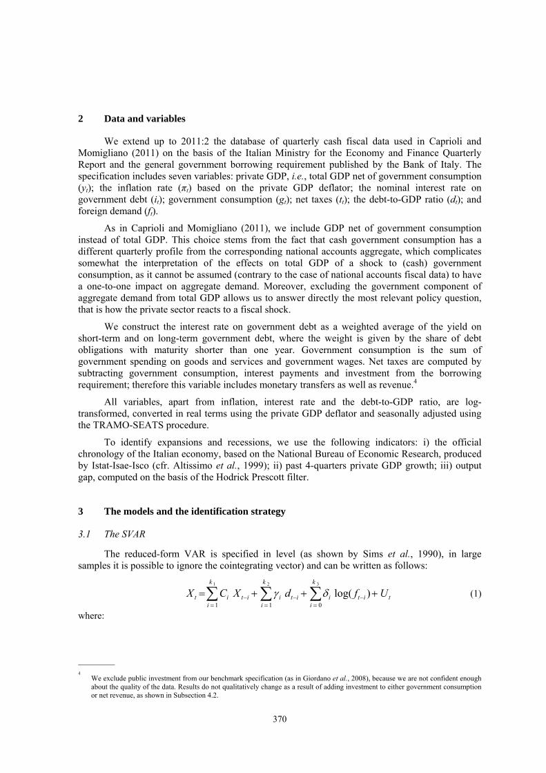
We extend up to 2011:2 the database of quarterly cash fiscal data used in Caprioli and Momigliano (2011) on the basis of the Italian Ministry for the Economy and Finance Quarterly Report and the general government borrowing requirement published by the Bank of Italy. The specification includes seven variables: private GDP, i.e., total GDP net of government consumption (yt); the inflation rate (πt) based on the private GDP deflator; the nominal interest rate on government debt (it); government consumption (gt); net taxes (tt); the debt-to-GDP ratio (dt); and foreign demand (ft).

As in Caprioli and Momigliano (2011), we include GDP net of government consumption instead of total GDP. This choice stems from the fact that cash government consumption has a different quarterly profile from the corresponding national accounts aggregate, which complicates somewhat the interpretation of the effects on total GDP of a shock to (cash) government consumption, as it cannot be assumed (contrary to the case of national accounts fiscal data) to have a one-to-one impact on aggregate demand. Moreover, excluding the government component of aggregate demand from total GDP allows us to answer directly the most relevant policy question, that is how the private sector reacts to a fiscal shock.

We construct the interest rate on government debt as a weighted average of the yield on short-term and on long-term government debt, where the weight is given by the share of debt obligations with maturity shorter than one year. Government consumption is the sum of government spending on goods and services and government wages. Net taxes are computed by subtracting government consumption, interest payments and investment from the borrowing requirement; therefore this variable includes monetary transfers as well as revenue.4

All variables, apart from inflation, interest rate and the debt-to-GDP ratio, are log-transformed, converted in real terms using the private GDP deflator and seasonally adjusted using the TRAMO-SEATS procedure.

To identify expansions and recessions, we use the following indicators: i) the official chronology of the Italian economy, based on the National Bureau of Economic Research, produced by Istat-Isae-Isco (cfr. Altissimo et al., 1999); ii) past 4-quarters private GDP growth; iii) output gap, computed on the basis of the Hodrick Prescott filter.

3 The models and the identification strategy

3.1 The SVAR

The reduced-form VAR is specified in level (as shown by Sims et al., 1990), in large samples it is possible to ignore the cointegrating vector) and can be written as follows:

(1) where:

————— 4 We exclude public investment from our benchmark specification (as in Giordano et al., 2008), because we are not confident enough

about the quality of the data. Results do not qualitatively change as a result of adding investment to either government consumption or net revenue, as shown in Subsection 4.2.

t

k

iiti

k

iiti

k

iitit UfdXCX

321

011

)log(

371

(2)

k1, k2 and k3 are the number of lags for the variables included in the VAR, for the debt-to-GDP ratio and for the foreign demand variable respectively.

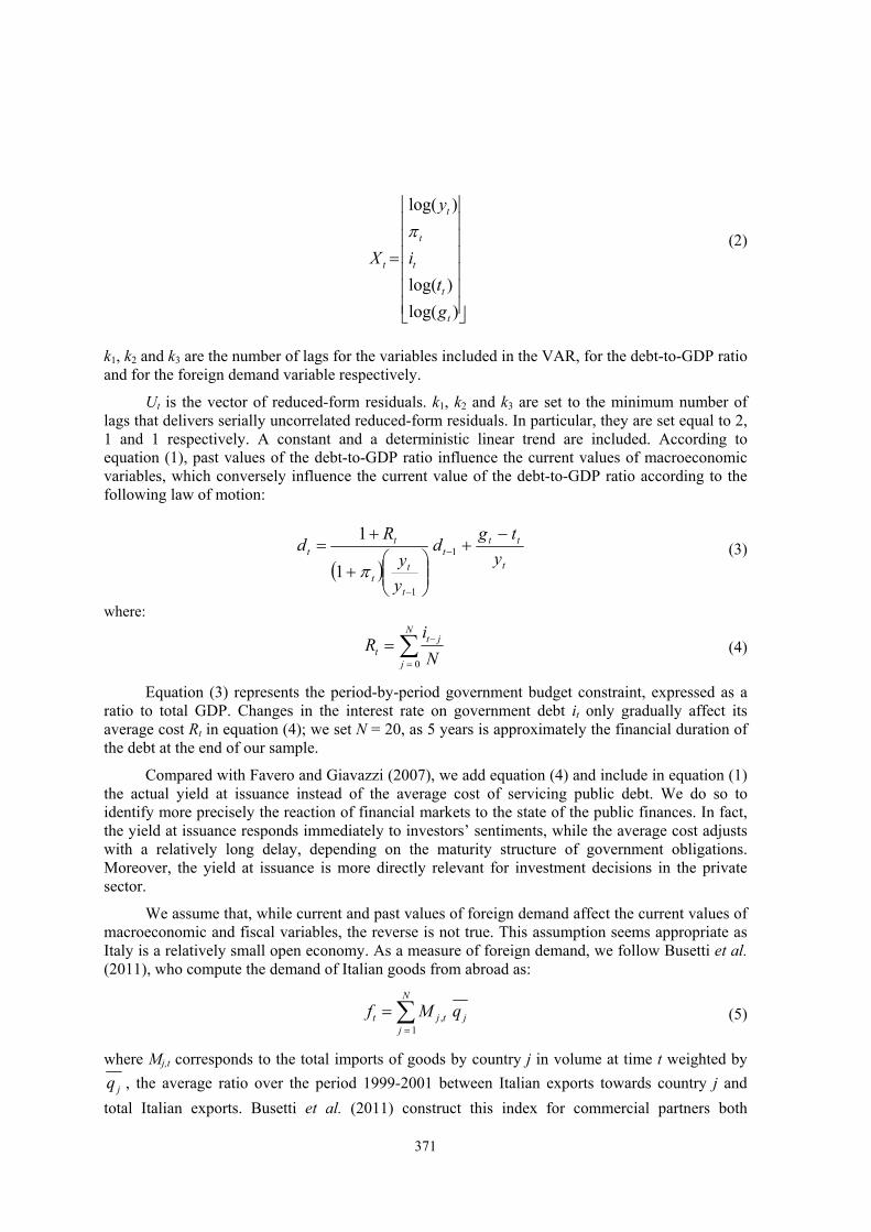
Ut is the vector of reduced-form residuals. k1, k2 and k3 are set to the minimum number of lags that delivers serially uncorrelated reduced-form residuals. In particular, they are set equal to 2, 1 and 1 respectively. A constant and a deterministic linear trend are included. According to equation (1), past values of the debt-to-GDP ratio influence the current values of macroeconomic variables, which conversely influence the current value of the debt-to-GDP ratio according to the following law of motion:

(3)

where: (4)

Equation (3) represents the period-by-period government budget constraint, expressed as a

ratio to total GDP. Changes in the interest rate on government debt it only gradually affect its average cost Rt in equation (4); we set N = 20, as 5 years is approximately the financial duration of the debt at the end of our sample.

Compared with Favero and Giavazzi (2007), we add equation (4) and include in equation (1) the actual yield at issuance instead of the average cost of servicing public debt. We do so to identify more precisely the reaction of financial markets to the state of the public finances. In fact, the yield at issuance responds immediately to investors’ sentiments, while the average cost adjusts with a relatively long delay, depending on the maturity structure of government obligations. Moreover, the yield at issuance is more directly relevant for investment decisions in the private sector.

We assume that, while current and past values of foreign demand affect the current values of macroeconomic and fiscal variables, the reverse is not true. This assumption seems appropriate as Italy is a relatively small open economy. As a measure of foreign demand, we follow Busetti et al. (2011), who compute the demand of Italian goods from abroad as:

(5)

where Mj,t corresponds to the total imports of goods by country j in volume at time t weighted by

jq , the average ratio over the period 1999-2001 between Italian exports towards country j and

total Italian exports. Busetti et al. (2011) construct this index for commercial partners both

)log(

)log(

)log(

t

t

t

t

t

t

g

t

i

y

X

t

ttt

t

tt

tt y

tgd

y

y

Rd

1

1

1

1

N

j

jtt N

iR

0

N

jjtjt qMf

1,

372

belonging to the Euro area and outside the EU. As a measure of global foreign demand, we consider the sum of the two indices.5

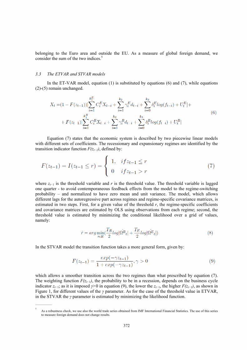
3.3 The ETVAR and STVAR models

In the ET-VAR model, equation (1) is substituted by equations (6) and (7), while equations (2)-(5) remain unchanged.

Equation (7) states that the economic system is described by two piecewise linear models with different sets of coefficients. The recessionary and expansionary regimes are identified by the transition indicator function F(zt−1), defined by:

where zt−1 is the threshold variable and r is the threshold value. The threshold variable is lagged one quarter - to avoid contemporaneous feedback effects from the model to the regime-switching probability – and normalized to have zero mean and unit variance. The model, which allows different lags for the autoregressive part across regimes and regime-specific covariance matrices, is estimated in two steps. First, for a given value of the threshold r, the regime-specific coefficients and covariance matrices are estimated by OLS using observations from each regime; second, the threshold value is estimated by minimizing the conditional likelihood over a grid of values, namely:

In the STVAR model the transition function takes a more general form, given by:

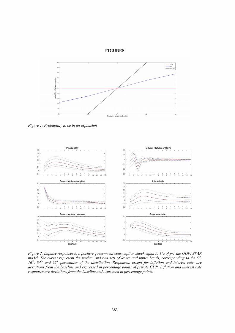
which allows a smoother transition across the two regimes than what prescribed by equation (7). The weighting function F(zt−1), the probability to be in a recession, depends on the business cycle indicator zt−1; as it is imposed γ>0 in equation (9), the lower the zt−1, the higher F(zt−1), as shown in Figure 1, for different values of the γ parameter. As for the case of the threshold value in ETVAR, in the STVAR the γ parameter is estimated by minimizing the likelihood function.

————— 5 As a robustness check, we use also the world trade series obtained from IMF International Financial Statistics. The use of this series

to measure foreign demand does not change results.

373

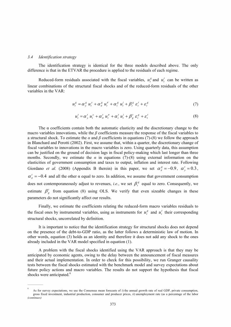
3.4 Identification strategy

The identification strategy is identical for the three models described above. The only difference is that in the ETVAR the procedure is applied to the residuals of each regime.

Reduced-form residuals associated with the fiscal variables, gtu and t

tu can be written as

linear combinations of the structural fiscal shocks and of the reduced-form residuals of the other variables in the VAR:

(7)

(8)

The α coefficients contain both the automatic elasticity and the discretionary change to the

macro variables innovations, while the β coefficients measure the response of the fiscal variables to a structural shock. To estimate the α and β coefficients in equations (7)-(8) we follow the approach in Blanchard and Perotti (2002). First, we assume that, within a quarter, the discretionary change of fiscal variables to innovations in the macro variables is zero. Using quarterly data, this assumption can be justified on the ground of decision lags in fiscal policy-making which last longer than three months. Secondly, we estimate the α in equations (7)-(8) using external information on the elasticities of government consumption and taxes to output, inflation and interest rate. Following

Giordano et al. (2008) (Appendix B therein) in this paper, we set 9.0g , 3.0t

y ,

4.0t and all the other α equal to zero. In addition, we assume that government consumption

does not contemporaneously adjust to revenues, i.e., we set gt equal to zero. Consequently, we

estimate tg from equation (8) using OLS. We verify that even sizeable changes in these

parameters do not significantly affect our results.

Finally, we estimate the coefficients relating the reduced-form macro variables residuals to

the fiscal ones by instrumental variables, using as instruments for gtu and t

tu their corresponding

structural shocks, uncorrelated by definition.

It is important to notice that the identification strategy for structural shocks does not depend on the presence of the debt-to-GDP ratio, as the latter follows a deterministic law of motion. In other words, equation (3) holds as an identity and therefore it does not add any shock to the ones already included in the VAR model specified in equation (1).

A problem with the fiscal shocks identified using the VAR approach is that they may be anticipated by economic agents, owing to the delay between the announcement of fiscal measures and their actual implementation. In order to check for this possibility, we run Granger causality tests between the fiscal shocks estimated with the benchmark model and survey expectations about future policy actions and macro variables. The results do not support the hypothesis that fiscal shocks were anticipated.6

————— 6 As for survey expectations, we use the Consensus mean forecasts of i) the annual growth rate of real GDP, private consumption,

gross fixed investment, industrial production, consumer and producer prices, ii) unemployment rate (as a percentage of the labor (continues)

gt

tt

gt

it

git

gyt

gy

gt uuuu

tt

gt

tg

it

tit

tyt

ty

tt uuuu

374

4 The effects of government consumption shocks in a SVAR model

Figure 2 show the response of the fiscal and macroeconomic variables to an exogenous shock (equal to 1% of private GDP) to government consumption in our benchmark model. In each panel the solid line represents the median response, while the dashed lines represent two sets of lower and upper bands, corresponding to the 5th, 16th, 84th and 95th percentiles of the distribution of the responses at each horizon, as commonly done in the literature.7

Concerning the reaction of fiscal variables, two points are worth mentioning. The first is that the government consumption shock is largely short-lived, being equal to 0.1% of private GDP already after four quarters. The second is that the higher public consumption is rapidly financed by higher revenues, which increase already in the first quarter, remain broadly constant at 0.2% of GDP for two years and then slowly decrease. The rise in net revenue, ensuring that the initial surge in the debt is fully absorbed within three years, reflects their direct stabilizing discretionary reaction to the debt and, to a lesser extent, to the increase in private GDP (see below).

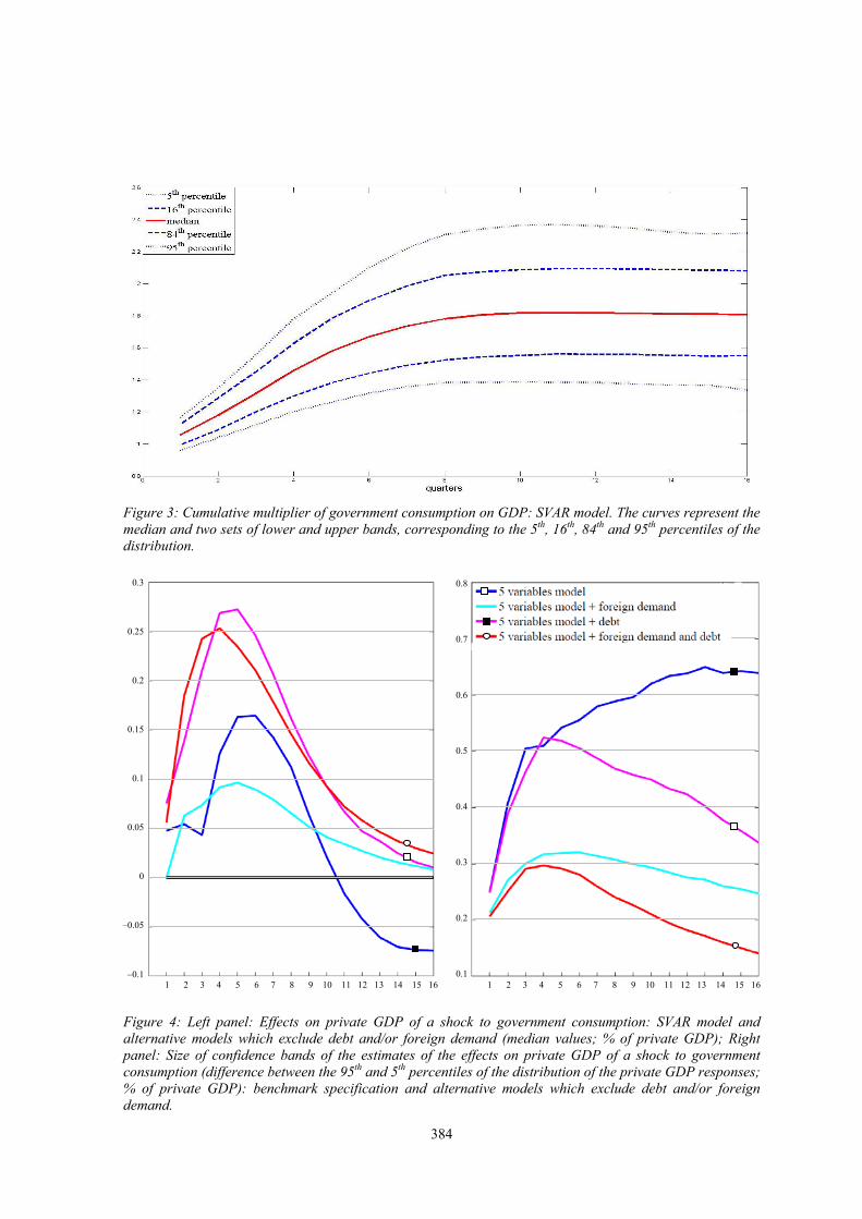
After a shock to public consumption, the response of private GDP is positive and highly significant for approximately two years. The peak, reached at the fourth quarter, is equal to 0.25% of GDP. Positive and significant effects of government consumption shocks on economic activity represent a relatively common result of the VAR literature (e.g., Giordano et al., 2008; Perotti, 2004; Mountford and Uhlig, 2002; and Neri, 2001). The output response to government consumption reflects the low persistence of the shock. To make our results more directly comparable with analyses which focus on total GDP (instead of its private component) and analyze shocks with a different persistence, we compute the cumulative multiplier (i.e., the ratio of the cumulative change in total GDP to the cumulative change in total government consumption)8 charted in Figure 3. The median value is equal to 1.04 on impact, reaches its peak (1.8) after three years and remains roughly constant thereafter. The confidence bands are relatively narrow compared with similar studies, with the 95th and the 5th percentiles of the distribution remaining above 1.3 and below 2.4 after the fifth quarter.

The median value for the long-run fiscal multiplier lies in the upper part of the wide range of estimates provided by the empirical literature. As shown in Spilimbergo et al. (2009), the relatively high value of the multiplier may be due to the debt-stabilizing reaction of fiscal variables. The transitory nature of the government consumption shock, rapidly compensated by higher revenues, and the small – and delayed – increase in interest rates do not pose a threat to the sustainability of the Italian public debt, notwithstanding its high level, making any precautionary savings by households unnecessary. The response of private GDP is robust across alternative specifications of the model.9

force), current account and state sector budget balance, and iii) three-month euro-area interest rate and 10-year Italian government bond yield. Following Ramney (2008) and Kirchner et al. (2010a), the fiscal shocks at time t are regressed on a constant, its own lag and the previous forecasts made in period t–1 for period t.

7 We compute confidence bands for IRF by bootstrapping. After estimating equation (1), we obtain fitted residuals Tuu ˆ,...,ˆ1

normally distributed with zero mean and covariance matrix Ω. We draw errors from this distribution to simulate the system of equations (1)-(5) L times. For each draw we compute the IRF as described in the previous footnote. Finally, we collect the αth and 1–αth percentile across the 1000 draws.

8 Following Giordano et al. (2008), we compute total GDP in this context by adding the cash-based government consumption

included in the model to private GDP. 9 As robustness checks, we considered the following model specifications in which: i) we include the interest rate only on debt

obligations with a maturity shorter than one year; ii) we use the gross yield on debt obligations with a maturity longer than three (continues)

375

The reaction of inflation to a government consumption shock is not statistically significant. This is in line with the analyses of Marcellino (2006), King and Plosser (1985) and Henry et al. (2004). The response of interest rates is relatively small, hump-shaped and never statistically significant. The existence of a positive relationship between interest rates and the level of government debt can be found in many empirical studies (see Bernheim, 1987, 1989; Gale and Orzag, 2002; Miller and Russek, 1996; and Engen and Hubbard, 2004).10

4.1 The role of government debt and foreign demand

The model includes two additional variables – government debt and foreign demand – with respect to the standard model found in the literature (5 variables: private GDP, inflation, interest rates, net revenue and government consumption). The inclusion of debt is important because it allows to better understand the fiscal framework associated with the shock. In particular, the reaction of fiscal variables – namely, government spending and net revenue – to changes in public debt can be analyzed.11 Empirical evidence (see Bohn, 2007; Trehan and Walsh, 1991; Hamilton and Flavin, 1986; and Golinelli and Momigliano, 2008) suggests that this feedback effect is generally important. In the case of a high-debt country like Italy, the influence of debt on the fiscal authorities’ decisions is likely to be particularly large.12 The inclusion of foreign demand is warranted by its strong influence on economic activity, Italy being a small open economy. As it can be safely assumed that foreign demand, measured by world demand, is not significantly influenced by Italian macro or fiscal variables, its inclusion in the VAR comes at a relatively small cost in terms of additional parameters to be estimated.

The left and right panels of Figure 4 show the impact of including public debt and/or foreign demand in the model respectively on the median response of private GDP and on the accuracy of this estimate, measured by the distance between the 95th and the 5th percentiles of the distribution.

Compared with a five-variable model that excludes both public debt and foreign demand, adding public debt determines a stronger (twice larger on average in the first two years) and longer lasting response of private GDP to a consumption shock (left panel). These results give support to the argument of Favero and Giavazzi (2007) that omitting debt in the model can result in biased estimates of the effects on GDP of fiscal shocks. The authors stressed the need to take into account the reactions of fiscal variables to changes in debt. In our case, these reactions would dampen the effects on output. On the contrary, we find a larger effect on private GDP, which comes from

years; iii) the specification of the VAR includes a quadratic trend instead of a linear one; iv) we include government investment in our definition of government consumption; v) net revenues come first when identifying the shocks (in the benchmark model, government consumption is ordered first); vi) the reduced-form residuals of fiscal variables depend explicitly on the level of government debt; and vii) the average financial duration is set equal to two years instead of its end-of-sample value (five years). We do not report these robustness checks, as estimates stay almost unchanged with respect to the benchmark specification. The results obtained with these alternative specifications confirm the hump-shaped pattern of private GDP and, apart from the “quadratic trend” specification for the quarters 6-10, they are well within the upper (95th percentile) and lower (5th percentile) bands of the GDP response in the benchmark specification. In the case of the “quadratic trend” specification, the lower impact on private GDP largely reflects the shorter persistence of the expenditure shock. The cumulative multiplier is very close to that for the benchmark specification.

10 The results for inflation and interest rates are also robust across the alternative specifications described in the previous footnote.

11 Recent research suggests that, depending on whether or not an expenditure shock is reabsorbed in the medium-long term, fiscal

multipliers may have different values (see Corsetti et al., 2009; and Ilzetzki et al., 2009). 12

Other researchers have included public debt in a SVAR exercise examining fiscal multipliers. We broadly follow the methodology of Favero and Giavazzi (2007), who add a deterministic equation linking debt dynamics to the government budget balance. Chung and Leeper (2007) employ a conceptually similar approach. Creel et al. (2005) include public debt as an additional variable. This second approach allows the analysis of the effects of direct shocks on government debt. This, however, comes at the cost of estimating a higher number of parameters than actually needed, as the government budget constraint is disregarded.

376

allowing a direct influence of debt on output.13 Adding also the foreign demand (so as to reach our benchmark specification) does not instead have a sizeable effect on the response of private GDP.

Compared with a five-variable model that excludes both public debt and foreign demand, adding public debt determines a very large improvement in the precision of estimates: the confidence band of the response shrinks almost to a third, on average (right panel of Figure 4). This is not a surprise, given its major influence on Italian macroeconomic developments. Adding the debt also improves the accuracy of the estimates further, but to a lesser extent.

5 Distinguishing across states of the economy: the effects of government consumption shocks

Compared to the analysis presented in Section 4, here we estimate the effects of expenditure shocks distinguishing between states of the economy. There is no consensus in the literature on the most appropriate indicator for the business cycle. The official chronology of the Italian economy (Altissimo et al., 1999; Istat, 2011) which follows the methodology followed in the US by the National Bureau of Economic Research, identifies 28 quarters (out of 118) as “recessions” in the period 1982-2011. We label the other periods as “expansions”. As a dichotomy variable cannot be used in the ETVAR and STVAR models, we employ as business cycle indicators the 4-quarters private GDP growth and the output gap, measured by the difference between the private GDP and its H.P. filter.

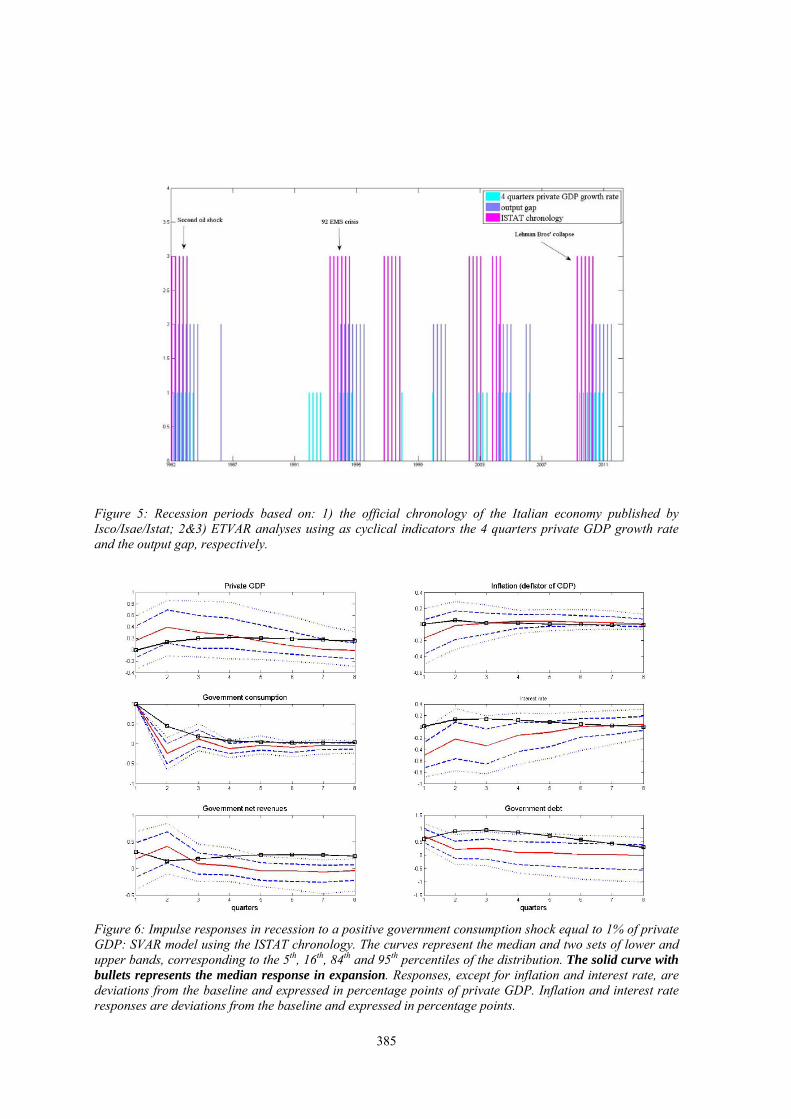
Figure 5 shows the recession periods based on the official chronology and those identified by the ETVAR model using the alternative indicators just mentioned. The ETVAR-based recessions are generally shifted forward with respect to the official chronology. Also, with ETVAR, the sample is more evenly split between the two regimes.

Nevertheless, Figure 5 allows to readily identify the four major recessions in our sample: the one at the beginning of the eighties, triggered by the second oil shock; the one at the beginning of the nineties, determined by the financial crisis; the strong slowdown in the initial years of the last decade and, finally, the last episode, influenced by the Lehman Bros’ collapse.

5.1 Identifying recessions on the basis of the official chronology of the Italian economy

Figures 6 and 7 show the response of the fiscal and macroeconomic variables to a government consumption shock in the recession periods identified by the official chronology and in the other periods (“expansions”), respectively. As in the IRFs previously discussed, the shock is equal to 1% of private GDP and the solid line represents the median response, while the dashed lines represent the 5th, 16th, 84th and 95th percentiles of the distribution of the responses.

When constructing impulse responses for a given regime, we assume that the state of the economy when the shock occurs does not change; in particular, we ignore any feedback effect from the fiscal shock to the type of regime. As this assumption becomes stronger the more we extend the time horizon of our analysis, we narrow it to 8 quarters in these IRFs and in the following ones.

The results are relatively close to those described in Section 4: in both regimes, the response of private GDP is positive and hump-shaped; revenues show a positive reaction making the initial surge in the debt to be gradually absorbed. However, under the recession regime, the response of ————— 13

Another possible explanation for the greater response of private GDP could be that the inclusion of debt led to a better identification of the exogenous fiscal shocks (as the endogenous reactions of fiscal variables to changes in debt were excluded). However, we compared estimated fiscal shocks obtained with and without debt and differences were negligible.

377

private GDP is more prompt (the peak effect of 0.4% is reached in the second quarter) and stronger on average in the first year. The response fades faster than in the expansion regime, but this is due to the fact that the expenditure shock goes to zero already in the second quarter, while in the expansion it diminishes more gradually.

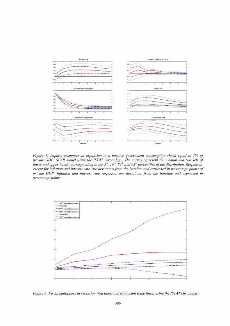
Figure 8 compares the cumulative multiplier in the two regimes. In recessions, the median multiplier is constantly higher than in expansions; however, due to the very large confidence bands in the recession regime, the two bands largely overlap (note that the graph includes only one standard deviation bands), indicating that the difference between the two estimates is not statistically significant.

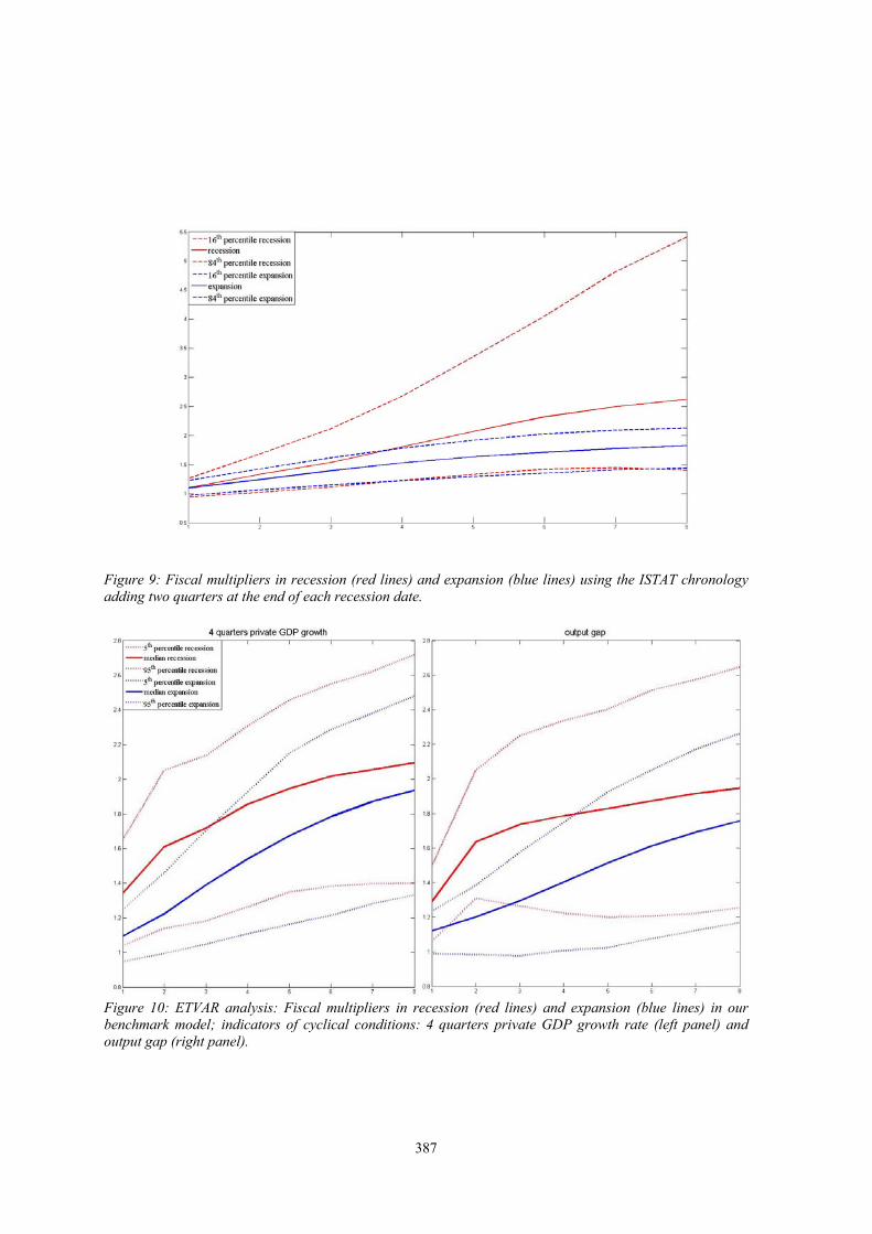
The very large size of the confidence bands estimated in the recession regime reflects the limited number of observations for this regime in the official chronology. To try to overcome this problem, we also run the SVAR adding to each recession the semester following it, as it is likely that substantial slack remains at the start of a recovery (in this way the number of observations for recessions increases to 40). This change improves the precision of estimates (in particular, the effects on private GDP in recession becomes statistically significant for 4 quarters) and reduces, but it does not eliminate, the overlap between the confidence bands of the estimates of the multipliers (Figure 9).

5.2 Identifying recessions on the basis of an ETVAR

While in the previous analysis recessions and expansions were identified outside the model, in this section the two regimes are endogenously identified in the ETVAR model on the basis of our indicators of cyclical conditions. The expenditure multipliers are reported in Figure 10. Results broadly confirm the analysis based on the official chronology: under the recession regime, the response of private GDP is more prompt and stronger. Compared to the previous analysis, the estimates for the recession regime (which includes 32 and 45 observations for the private GDP growth rate and the output gap respectively) are more accurate, but there is still a large overlap between the confidence bands of the fiscal multipliers. In order to overcome the problem of the limited number of observations in each sub-sample, we estimate the 3-variable model (namely, private GDP, government consumption and net revenue) originally proposed in Blanchard and Perotti (2002), which is more parsimonious than our benchmark model in terms of number of parameters to be estimated; in this case the difference across fiscal multipliers in the two regimes is positive and statistically significant (1-standard-deviation confidence bands do not overlap), but only using the 4-quarter private GDP growth rate (Figure 11).

5.3 Identifying recessions on the basis of an STVAR

In the previous two sections, the sample was split into two regimes (recessions and expansions) and two sets of parameters were estimated. The STVAR model allows instead a smooth transition between the two regimes; in each quarter the parameters of the model are a linear combination of two sets of values (corresponding to each regime), weighted by the degree of being in each regime (Auerbach and Gorodnichenko, 2012).

In order to produce IRFs with this approach (and also to identify fiscal multipliers), we need to select two benchmarks, representative for recessions and expansions. We select the benchmarks so to leave outside them 20 per cent of the observations. For the 4-quarter moving average of the private GDP annualized growth rate, these benchmarks corresponds to, respectively, –2,5 and 1.5. Figure 12 shows that the estimated degree of being in recession increases in those periods identified as recessions on the basis of the official chronology, especially when using the 4-quarters

378

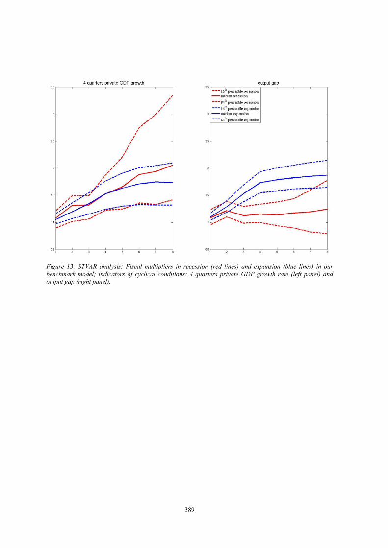
private GDP growth. The estimates of the expenditure multipliers are reported in Figure 13. Results are far less clear-cut than in the previous analysis. Depending on the cyclical indicator used, in recessions the expenditure multiplier is constantly higher (4-quarters private GDP growth) or constantly lower (output gap). Estimates are generally less precise than those obtained with the ETVAR model, as shown by the larger confidence bands compared to those in Figure 10 (imprecise estimates, not reported, are also obtained in the case of the 3-variable model).

8 Conclusions and future research

In this paper we study how the effects of expenditure shock on economic activity are influenced by the state of the economy on the basis of various autoregressive models and two commonly used indicators of cyclical conditions. We rely on quarterly cash-basis fiscal data for the Italian economy covering the period 1982:1-2011:2.

The main results can be summarized as follows.

Independently of the method that we use and whether we distinguish or not between states of the economy, the expenditure shocks that we estimate tend to be largely transitory and revenues show a positive reaction, making the initial surge in the debt to be gradually absorbed.

In the analysis which doesn’t take into account the state of the economy, the response of private GDP to an expenditure shock is positive and highly significant for approximately two years. The government consumption multiplier (1.04 on impact and 1.8 at the peak) lies in the upper part of the wide range of estimates provided by the empirical literature.14

When we split the sample in “expansion” and “recession” regimes, either on the basis of the official chronology or applying the ETVAR approach, the regime-specific IRFs are broadly similar to those estimated for the full sample but generally less precise. Under the recession regime, the response of private GDP is larger and more prompt; the cumulative multiplier is also stronger on average. However, the confidence bands of the estimates are relatively large, and the difference in the median across regimes is not statistically significant. Only using a more parsimonious model and the private GDP growth rate as indicator of cyclical conditions the differences across regimes are statistically significant.

Median results are less clear-cut when we estimate the STVAR model: in recession the median value of the expenditure multiplier is higher or lower depending on the cyclical indicator used,. This result is associated to estimates that are even less precise than those obtained with the ETVAR approach. This is somewhat unexpected, as this method is deemed to use more efficiently the information of the sample; a possible explanation is that weighting function F(zt−1), in the presence of highly imperfect indicators of cyclical conditions, represents a sort of unwarranted straightjacket for the data.

Results do not seem to give a clear support to the idea that higher multipliers may be due, at least partly, to a different behaviour of interest rates, as their response differs across methods and indicators; also the negative wealth effect (Barro, 1982) and/or the credit-crunch channel associated to public debt during recessions (De Bonis and Stacchini, 2009) can lower the direct stimulus provided to the economic activity by higher public consumption.

————— 14

This may be due to the debt-stabilizing reaction of revenues, in line with the idea that the effects of fiscal stimulus on economic activity depend positively on the soundness of fiscal policy (see, e.g., Corsetti et al., 2009). The transitory nature of the shocks that we observe and their small size may also have a bearing on the value of the multiplier.

379

In conclusion, our empirical investigation shows some weak evidence that expenditure multipliers tend to be higher in recessions than in expansions. While this result is influenced by the limited size of the sub-samples, it seems to suggest that the differences in the multipliers have not been extremely large, at least in the period under examination.

Finally, our empirical analysis could be strengthened along at least two lines. First, the assumption that the initial state of the economy does not change when constructing impulse responses for a given regime should be relaxed. Second, a more thorough selection and discussion of business cycle indicators should be conducted.

380

REFERENCES

Altissimo, F., Marchetti, D. J., Oneto, G. P.: 2000, “The Italian Business Cycle: Coincident and Leading Indicators and Some Stylized Facts”, Banca d’Italia, Temi di Discussione, No. 377.

Auerbach, A. and Gorodnichenko, Y.: 2012, “Measuring the Output Responses to Fiscal Policy”, American Economic Journal: Economic Policy, forthcoming.

Barro, R.: 1974, Are Government Bonds Net Wealth?, Journal of Political Economy, Vol. 82, No.6.

Baum, A. and Koester, G.: 2011, “The Impact of Fiscal Policy on Economic Activity Over the Business Cycle – Evidence from a Threshold VAR Analysis”, Deutsche Bundesbank, Discussion Paper, No. 03/2011.

Baum, A., Poplawski-Ribeiro, M. and Weber, A.: 2012, “Fiscal Multipliers and the State of the Economy”, IMF, Working Paper, forthcoming.

Bernheim, B. D.: 1987, “Ricardian Equivalence: An Evaluation of Theory and Evidence”, NBER Macroeconomic Annual, Cambridge: MIT Press, pp. 263-304.

Blanchard, O. and Perotti, R.: 2002, “An Empirical Characterization of the Dynamic Effects of Changes in Government Spending and Taxes on Output”, Quarterly Journal of Economics, No. 117.

Bohn, H.: 2007, “Are Stationarity and Cointegration Restrictions Really Necessary for the Intertemporal Budget Constraint?”, Journal of Monetary Economics, No. 54, pp. 1837-47.

Burriel, P., de Castro, F., Garrote, D., Gordo, E., Paredes, J. and Perez, J.: 2010, “Fiscal Policy Shocks in the Euro Area and the US: An Empirical Assessment”, ECB, Working Paper, No. 1133.

Busetti, F., Felettigh, A. and Tedeschi, R.: 2011, “Esportazioni italiane e domanda potenziale all’interno e all’esterno dell’area dell’euro: Stime econometriche disaggregate e uno scenario Controfattuale”, Banca d’Italia, mimeo.

Caprioli, F. and Momigliano, S.: 2011, “The Effects of Fiscal Shocks with Debt-stabilizing Budgetary Policies in Italy”, Banca d’Italia, Temi di Discussione, No. 839.

Chahrour, C., Schmitt-Grohe, S. and Uribe, M.: 2010, “A Model-based Evaluation of the Debate on the Size of Tax Multiplier”, NBER, Working Paper, No. 16169.

Christiano, L., Eichenbaum, M. and Rebelo, S.: 2009, “When is the Government Spending Multiplier Large?”, Northwestern University, manuscript.

Chung, H. and Leeper, E. M.: 2007, “What Has Financed Government Debt”, University of Indiana, manuscript.

Coenen, G., Erceg, C., Freedman, C., Furceri, D., Kumhof, M., Lalonde, R., Laxton, D., Lindé, J., Mourougane, A., Muir, D., Murusula, S., de Resende, C., Roberts, J., Roeger, W., Snudden, S., Trabandt, M. and in’t Veld, J.: 2010, “Effects of Fiscal Stimulus in Structural Models”, IMF, Working Paper, No. 10/73.

Cogan, J., Cwik, T., Wieland, V. and Taylor, J.: 2009, “New Keynesian Versus Old Keynesian Government Spending Multipliers”, ECB, Working Paper, No. 1090.

Corsetti, G., Meier, A. and Mueller, G.: 2009, “Fiscal Stimulus with Spending Reversal”, IMF, Working Paper, No. 09106.

Corsetti, G., Meier, K. and Mueller, G.: 2010, “Debt Consolidation and Fiscal Stabilization of Deep Recessions”, American Economic Review, No. 100, pp. 41-45.

381

Creel, J., Monperrus-Veroni, P. and Saraceno, F.: 2005, “Discretionary Policy Interactions and the Fiscal Theory of the Price Level: A SVAR Analysis on French Data”, OFCE, Document de travail, No. 12.

De Bonis, R. and Stacchini, M.: 2009, “What Determines the Size of Bank Loans in Industrialized Countries? The Role of Government Debt”, Banca d’Italia, Temi di Discussione, No. 707.

Edelberg, W., Eichenbaum, M. and Fisher, J.: 1999, “Understanding the Effects of a Shock to Government Purchases”, Review of Economic Dynamics, No. I (January), pp. 166-206.

Engen, E. and Hubbard, R. G.: 2004, “Federal Government Debts and Interest Rates”, NBER, Working Paper, No. 1068, pp. 1419-31.

Fatás, A. and Mihov, I.: 2001, “The Effects of Fiscal Policy on Consumption and Employment: Theory and Evidence”, CEPR, Discussion Paper, No. 2760.

Fazzari, S.M., Morley, J. and Panovska, I.: 2012, “State Dependent Effects of Fiscal Policy, mimeo.

Favero, C. and Giavazzi, F.: 2007, “Debt and the Effect of Fiscal Policy”, NBER, Working Paper, No. 12822.

Gale, W. G. and Orzag, P.: 2002, “The Economic Effects of Long-term Fiscal Discipline”, Urban Institute-Brookings Institution, Tax Policy Center, Discussion Paper, December.

Giordano, R., Momigliano, S., Neri, S. and Perotti, R.: 2008, “The Effects of Fiscal Policy in Italy: Evidence from a VAR Model”, European Journal of Political Economy, No. 23, pp. 707-33.

Golinelli, R. and Momigliano, S.: 2008, “The Cyclical Response of Fiscal Policies in the Euro Area. Why Do Results of Empirical Research Differ So Strongly?”, Banca d’Italia, Temi di Discussione, No. 654.

Hamilton, J. and Flavin, M.: 1986, “On the Limitations of Government Borrowing: A Framework for Empirical Testing”, American Economic Review, No. 76, pp. 808-19.

Henry, J., Hernández de Cos, P. and Momigliano, S.: 2004, “The Short-term Impact of Government Budgets on Prices: Evidence from Macroeconometric Models”, ECB, Working Paper, No. 396.

Hernández de Cos, P. and Moral-Benito, E.: 2013, “Fiscal Multipliers for Crisis Times: The Case of Spain”, Banco de España, mimeo.

Ilzetzki, E., Mendoza, E. and Vegh, C.: 2009, “How Big Are Fiscal Multipliers?”, CEPR, Policy Insight, No. 39.

IMF: 2012, World Economic Outlook.

ISTAT: 2010, Rapporto annuale: La situazione del paese nel 2010.

King, R. and Plosser, C.: 1985, “Money, Deficit and Inflation”, Carnagie Rochester Conference Series on Public Policy, No. 22, pp. 147-96.

Kirchner, M., Cimadomo, J. and Hauptmeier, S.: 2010a, “Transmission of Government Spending Shocks in the Euro Area: Time Variation and Driving Forces”, mimeo.

Marcellino, M.: 2006, “Some Stylized Facts on Non-systematic Fiscal Policy in the Euro Area”, Journal of Macroeconomics, No. 28, pp. 461-79.

Miller, S. M. and Russek, F. S.: 1996, “Do Federal Deficits Affect Interest Rates? Evidence from Three Econometric Methods”, Journal of Macroeconomics, No. 18, pp. 403-28.

382

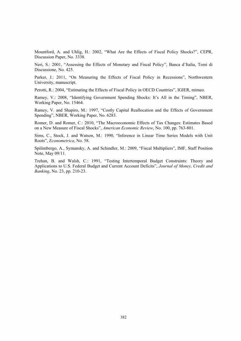
Mountford, A. and Uhlig, H.: 2002, “What Are the Effects of Fiscal Policy Shocks?”, CEPR, Discussion Paper, No. 3338.

Neri, S.: 2001, “Assessing the Effects of Monetary and Fiscal Policy”, Banca d’Italia, Temi di Discussione, No. 425.

Parker, J.: 2011, “On Measuring the Effects of Fiscal Policy in Recessions”, Northwestern University, manuscript.

Perotti, R.: 2004, “Estimating the Effects of Fiscal Policy in OECD Countries”, IGIER, mimeo.

Ramey, V.: 2008, “Identifying Government Spending Shocks: It’s All in the Timing”, NBER, Working Paper, No. 15464.

Ramey, V. and Shapiro, M.: 1997, “Costly Capital Reallocation and the Effects of Government Spending”, NBER, Working Paper, No. 6283.

Romer, D. and Romer, C.: 2010, “The Macroeconomic Effects of Tax Changes: Estimates Based on a New Measure of Fiscal Shocks”, American Economic Review, No. 100, pp. 763-801.

Sims, C., Stock, J. and Watson, M.: 1990, “Inference in Linear Time Series Models with Unit Roots”, Econometrica, No. 58.

Spilimbergo, A., Symansky, A. and Schindler, M.: 2009, “Fiscal Multipliers”, IMF, Staff Position Note, May 09/11.

Trehan, B. and Walsh, C.: 1991, “Testing Intertemporal Budget Constraints: Theory and Applications to U.S. Federal Budget and Current Account Deficits”, Journal of Money, Credit and Banking, No. 23, pp. 210-23.

383

FIGURES

Figure 1: Probability to be in an expansion

Figure 2: Impulse responses to a positive government consumption shock equal to 1% of private GDP: SVAR model. The curves represent the median and two sets of lower and upper bands, corresponding to the 5th, 16th, 84th and 95th percentiles of the distribution. Responses, except for inflation and interest rate, are deviations from the baseline and expressed in percentage points of private GDP. Inflation and interest rate responses are deviations from the baseline and expressed in percentage points.

384

Figure 3: Cumulative multiplier of government consumption on GDP: SVAR model. The curves represent the median and two sets of lower and upper bands, corresponding to the 5th, 16th, 84th and 95th percentiles of the distribution.

Figure 4: Left panel: Effects on private GDP of a shock to government consumption: SVAR model and alternative models which exclude debt and/or foreign demand (median values; % of private GDP); Right panel: Size of confidence bands of the estimates of the effects on private GDP of a shock to government consumption (difference between the 95th and 5th percentiles of the distribution of the private GDP responses; % of private GDP): benchmark specification and alternative models which exclude debt and/or foreign demand.

0.3

0.25

0.2

0.15

0.1

0.05

0

–0.05

–0.1 1 2 3 4 5 6 7 8 9 10 11 12 13 14 15 16 1 2 3 4 5 6 7 8 9 10 11 12 13 14 15 16

0.8

0.7

0.6

0.5

0.4

0.3

0.2

0.1

385

Figure 5: Recession periods based on: 1) the official chronology of the Italian economy published by Isco/Isae/Istat; 2&3) ETVAR analyses using as cyclical indicators the 4 quarters private GDP growth rate and the output gap, respectively.

Figure 6: Impulse responses in recession to a positive government consumption shock equal to 1% of private GDP: SVAR model using the ISTAT chronology. The curves represent the median and two sets of lower and upper bands, corresponding to the 5th, 16th, 84th and 95th percentiles of the distribution. The solid curve with bullets represents the median response in expansion. Responses, except for inflation and interest rate, are deviations from the baseline and expressed in percentage points of private GDP. Inflation and interest rate responses are deviations from the baseline and expressed in percentage points.

386

Figure 7: Impulse responses in expansion to a positive government consumption shock equal to 1% of private GDP: SVAR model using the ISTAT chronology. The curves represent the median and two sets of lower and upper bands, corresponding to the 5th, 16th, 84th and 95th percentiles of the distribution. Responses, except for inflation and interest rate, are deviations from the baseline and expressed in percentage points of private GDP. Inflation and interest rate responses are deviations from the baseline and expressed in percentage points.

Figure 8: Fiscal multipliers in recession (red lines) and expansion (blue lines) using the ISTAT chronology.

387

Figure 9: Fiscal multipliers in recession (red lines) and expansion (blue lines) using the ISTAT chronology adding two quarters at the end of each recession date.

Figure 10: ETVAR analysis: Fiscal multipliers in recession (red lines) and expansion (blue lines) in our benchmark model; indicators of cyclical conditions: 4 quarters private GDP growth rate (left panel) and output gap (right panel).

388

Figure 11: ETVAR analysis Fiscal multipliers in recession (red lines) and expansion (blue lines) in the 3-variable model; indicators of cyclical conditions: 4 quarters private GDP growth rate (left panel) and output gap (right panel).

Figure 12: Probability to be in a recession based on: 1) the official chronology of the Italian economy published by Isco/Isae/Istat; 2&3) STVAR analyses using as cyclical indicators the 4 quarters private GDP growth rate and the output gap, respectively.

389

Figure 13: STVAR analysis: Fiscal multipliers in recession (red lines) and expansion (blue lines) in our benchmark model; indicators of cyclical conditions: 4 quarters private GDP growth rate (left panel) and output gap (right panel).