1

READING 18: CAPITAL MARKET EXPECTATIONS

A- Organizing the Task: Framework and Challenges

1- A Framework for Developing Capital Market Expectations

The following is a framework for a disciplined approach to setting CME.

1. Specify the final set of expectations that are needed, including the time horizon to which

they apply.

2. Research the historical record.

3. Specify the method(s) and/or model(s) that will be used and their information

requirements.

4. Determine the best sources for information needs.

5. Interpret the current investment environment using the selected data and methods,

applying experience and judgment.

6. Provide the set of expectations that are needed, documenting conclusions.

7. Monitor actual outcomes and compare them to expectations, providing feedback to

improve the expectations-setting process.

The development of capital market expectations is beta research (research related to systematic risk

and returns to systematic risk). As such, it is usually centralized so that the CME inputs used across all

equity and fixed-income products are consistent. On the other hand, alpha research (research related to

capturing excess risk-adjusted returns by a particular strategy) is typically conducted within particular

product groups with the requisite investment-specific expertise.

2- Challenges in forecasting

a. Limitations of Economic Data

The analyst needs to understand the definition, construction, timeliness, and accuracy of any data

used, including any biases.

1. The time lag with which economic data are collected, processed, and disseminated can be

an impediment to their use.

2. One or more official revisions to the initial values are common. In effect, measurements are

made with error, but the direction and magnitude of the error are not known at the time

the data are initially publicized.

3. Definitions and calculation methods change too.

4. An analyst must realize that suppliers of indices of economic and financial data periodically

re-base these indices, meaning that the specific time period used as the base of the index

is changed. A re-basing is not a substantive change in the composition of an index. It is more

of a mathematical change. Analysts constructing a data series should take care that data

relating to different bases are not inadvertently mixed together.

2

b. Data Measurement Errors and Biases

Analysts need to be aware of possible biases in data measurement of series such as asset class returns.

Errors in data series include the following:

1. Transcription errors. These are errors in gathering and recording data. Such errors are most

serious if they reflect a bias.

2. Survivorship bias. Survivorship bias arises when a data series reflects only entities that have

survived to the end of the period.

3. Appraisal (smoothed) data. For certain assets without liquid public markets, appraisal data are

used in lieu of market price transaction data.

Appraised values tend to be less volatile than market-determined values for the identical asset

would be. The consequences are 1) the calculated correlations with other assets tend to be

smaller in absolute value than the true correlations, and 2) the true standard deviation of the

asset is biased downward. This concern has been raised particularly with respect to alternative

investments such as real estate.

The analyst can attempt to correct for the biases in datasets (when a bias-free dataset is not

available). For example, one heuristic approach to correcting for smoothed data is to rescale the data

in such a way that their dispersion is increased but the mean of the data is unchanged.

c. The Limitations of Historical estimates

A historical estimate should be considered a starting point for analysis. The analysis should include a

discussion of what may be different from past average results going forward. Changes in the

technological, political, legal, and regulatory environments, as well as disruptions such as wars and

other calamities, can alter risk–return relationships. Such shifts are known as changes in regime (the

governing set of relationships) and give rise to the statistical problem of nonstationarity.

When many variables are considered, a long data series may be a statistical necessity. If we could be

assured of stationarity, going back farther in time to capture a larger sample should increase the

precision with which population parameters of a return distribution are estimated.

Using larger samples may reduce the sensitivity of parameter estimates to the starting and ending dates

of the sample. In practice, using a long data series may involve a variety of problems. For instance:

The risk that the data cover multiple regimes increases.

Time series of the required length may not be available.

In order to get data series of the required length, the temptation is to use high- frequency data

(weekly or even daily). Data of high frequency are more sensitive to asynchronism across

variables. As a result, high-frequency data tend to produce lower correlation estimates.

The underlying mean returns on volatile asset classes such as equities are particularly difficult to

estimate from historical data. Using high-frequency data is of no help in increasing the accuracy of

mean return estimates.

3

d. Ex Post Risk Can Be a Biased Measure of Ex Ante Risk

In interpreting historical prices and returns over a given sample period for their relevance to current

decision making, we need to evaluate whether asset prices in the period reflected the possibility of a

very negative event that did not materialize during the period. Looking backward, we are likely to

underestimate ex ante risk and over- estimate ex ante anticipated returns.

e. Biases in Analysts Methods

The preventable biases that the analyst may introduce are the following:

Data-mining bias: introduced by repeatedly “drilling” or searching a dataset until the analyst

finds some statistically significant pattern. Such patterns cannot be expected to be of predictive

value.

Time-period bias. Time-period bias relates to results that are time period specific. Research

findings are often found to be sensitive to the selection of starting and/or ending dates.

The analyst should scrutinize the variable selection process for data-mining bias and be able to provide

an economic rationale for the variable’s usefulness in a forecasting mode. A further practical check is

to examine the forecasting relationship out of sample.

f. The failure to account for Conditioning Information

We observed above that the analyst should ask whether there are relevant new facts in the present

when forecasting the future. Where such information exists, the analyst should condition his or her

expectations on it.

Prospective returns and risk for an asset as of today are conditional on the specific characteristics of the

current marketplace and prospects looking forward. The use of unconditional expectations can lead to

misperceptions of risk, return, and risk-adjusted return. Example of asset beta that changes with

business cycle.

g. Misinterpretation of Correlations

In financial and economic research, the analyst should take care in interpreting correlations. When a

variable A is found to be significantly correlated with a variable B, there are at least three possible

explanations:

A predicts B;

B predicts A;

A third variable C predicts A and B.

Another surprise that might be in store: A and B could have a strong but nonlinear relationship

but have a low or zero correlation.

Without the investigation and modeling of underlying linkages, relationships of correlation cannot be

used in a predictive model.

4

h. Psychological Traps (revert to behavioral biases for more detail)

1. The anchoring trap is the tendency of the mind to give disproportionate weight to the first

information it receives on a topic.

2. The status quo trap is the tendency for forecasts to perpetuate recent observations—that is, to

predict no change from the recent past.

3. The confirming evidence trap is the bias that leads individuals to give greater weight or seek

information that supports an existing or preferred point of view than to evidence that

contradicts it. Several steps may be taken to help ensure objectivity:

o Examine all evidence with equal rigor.

o Enlist an independent-minded person to argue against your preferred conclusion or

decision.

o Be honest about your motives.

4. The overconfidence trap is the tendency of individuals to overestimate the accuracy of their

forecasts.

5. The prudence trap is the tendency to temper forecasts so that they do not appear extreme, or

the tendency to be overly cautious in forecasting.

6. The recallability trap is the tendency of forecasts to be overly influenced by events that have

left a strong impression on a person’s memory. To minimize the distortions of the recallability

trap, analysts should ground their conclusions on objective data and procedures rather than

on personal emotions and memories.

i. Model Uncertainty

The analyst usually encounters at least two kinds of uncertainty in conducting an analysis: model

uncertainty (uncertainty concerning whether a selected model is correct) and input uncertainty

(uncertainty concerning whether the inputs are correct).

These uncertainties make it hard to confirm the existence of capital market anomalies (inefficiencies);

some valuation model usually underlies the identification of an inefficiency. On the other hand,

behavioral finance has offered explanations for many perceived capital market anomalies.

B- Tools for Formulating Capital Market Expectations

1- Formal Tools

Formal tools are established research methods amenable to precise definition and independent

replication of results.

a. Statistical Methods

Statistical methods relevant to expectations setting include descriptive statistics (methods for

effectively summarizing data to describe important aspects of a dataset) and inferential statistics

(methods for making estimates or forecasts about a larger group from a smaller group actually

5

observed). The simplest approach to forecasting is to use past data to directly forecast future outcomes

of a variable of interest.

i. Historical Statistical Approach: Sample Estimators

A sample estimator is a formula for assigning a unique value (a point estimate) to a population

parameter. For example, in a mean–variance framework, the analyst might use:

the sample arithmetic mean total return or sample geometric mean total return as an estimate

of the expected return;

the sample variance as an estimate of the variance; and

sample correlations as estimates of correlations.

One decision point relates to the choice between an arithmetic mean and a geometric mean.

The arithmetic mean return (which is always used in the calculation of the sample standard

deviation) best represents the mean return in a single period.

The geometric mean return of a sample represents the compound rate of growth that equates

the beginning value to the ending value of a data series. The geometric mean return represents

multiperiod growth more accurately than the arithmetic mean return.

ii. Shrinkage Estimators

Shrinkage estimation involves taking a weighted average of a historical estimate of a parameter and

some other parameter estimate, where the weights reflect the analyst’s relative belief in the

estimates. This “two- estimates-are-better-than-one” approach has desirable statistical properties that

have given it a place in professional investment practice.

A shrinkage estimator of the covariance matrix is a weighted average of the historical covariance

matrix and another, alternative estimator of the covariance matrix, where the analyst places the

larger weight on the covariance matrix he or she believes more strongly in. Because investment data

series are relatively short and samples often reflect the nonrecurring peculiarities of a historical period.

The sample covariance matrix is perfectly well suited for summarizing an observed dataset and has the

desirable (large-sample) property of unbiasedness. Nevertheless, a shrinkage estimator is a superior

approach for estimating the population covariance matrix for the medium- and smaller-size datasets

that are typical in finance.

A shrinkage estimator approach involves selecting an alternative estimator of the covariance matrix,

called a target covariance matrix. A surprising fact concerning the shrinkage estimator approach is that

any choice for the target covariance matrix will lead to an increase (or at least not a decrease) in the

efficiency of the covariance estimates versus the historical estimate. The improvement will be greater

if a plausible target covariance matrix is selected. If the target covariance matrix is useless in

improving the accuracy of the estimate of covariance, the optimal weight on the historical estimate

would be calculated as 1. One reasonable choice for the target covariance matrix would be a factor-

model-based estimate of the covariance matrix. Another choice for the target covariance matrix would

be a covariance matrix based on assuming each pairwise covariance is equal to the overall average

covariance.

6

iii. Time-Series Estimators

Time-series estimators involve forecasting a variable on the basis of lagged values of the variable

being forecast and often lagged values of other selected variables.

Time-series methods have been found useful in developing particularly short-term forecasts for

financial and economic variables. Time-series methods have been notably applied to estimating near-

term volatility, given persuasive evidence of variance clustering in a number of different markets,

including equity, currency, and futures markets.

Volatility clustering is the tendency for large/small swings in prices to be followed by large/small swings

of random direction; it captures the idea that markets represent periods of notably high or low volatility.

Example of a simple model

𝝈𝒕𝟐 = 𝜷𝝈𝒕−𝟏

𝟐 + (𝟏 − 𝜷)𝜺𝒕𝟐

This model specifies that the volatility in period 𝑡, 𝜎𝑡2, is a weighted average of the volatility in the

previous period, 𝜎𝑡−12 , and the squared value of a random “noise” term, 𝜀𝑡

2.

iv. Multifactor Models

A multifactor model explains the returns to an asset in terms of the values of a set of return drivers or

risk factors. The structure, if the analyst believes that K factors drive asset returns, is as follows:

𝑹𝒊 = 𝒂𝒊 + 𝒃𝒊𝟏𝑭𝟏 + 𝒃𝒊𝟐𝑭𝟐 + ⋯ + 𝒃𝒊𝑲𝑭𝑲 + 𝜺𝒊

Where,

𝑹𝒊= the return to asset i

𝒂𝒊= an intercept term in the equation for asset i

𝑭𝑲= the return to factor k, k=1,2,...,K

𝒃𝒊𝑲= the sensitivity of the return to asset i to the return to factor k

𝜺𝒊= an error term with a zero mean that represents the portion of the

return to asset i not explained by the factor model.

This structure has been found useful for modeling asset returns and covariances among asset returns.

Multifactor models are useful for estimating covariances for the following reasons:

By relating the returns on all assets to a common set of return drivers, a multifactor model

simplifies the task of estimating covariances: estimates of covariances between asset returns

can be derived using the assets’ factor sensitivities.

When the factors are well chosen, a multifactor model approach may filter out noise

Such models make it relatively easy to verify the consistency of the covariance matrix,

because if the smaller factor covariance matrix is consistent, so are any covariances computed

on the basis of it.

Equation - 2

Equation - 1

7

A factor covariance matrix contains the covariances for the factors assumed to drive returns.

The asset covariance matrix is the covariance matrix for the asset classes or markets under

consideration, to calculate it we need to know how each of the markets responds to factor movements.

We measure the responsiveness of markets to factor movements by the markets’ factor sensitivities

(also known as factor betas or factor loadings), represented by the quantities 𝑏𝑖𝐾 in Equation 2.

In addition, every market has some risk that is not explained by the factors called the market’s

idiosyncratic or residual risk and represented by the residual variance, Var(𝜀𝑖) for market 𝑖.

In the case that is examined, we are assuming that the return of market, 𝑀𝑖 is as follows:

𝑴𝒊 = 𝒂𝒊 + 𝒃𝒊𝟏𝑭𝟏 + 𝒃𝒊𝟐𝑭𝟐 + 𝜺𝒊

We compute the markets’ variances and covariance using Equations 3a and 3b, respectively:

𝑴𝒊𝒊 = 𝒃𝒊𝟏𝟐 𝑽𝒂𝒓(𝑭𝟏) + 𝒃𝒊𝟐

𝟐 𝑽𝒂𝒓(𝑭𝟐) + 𝟐𝒃𝟏𝒊𝒃𝟐𝒊𝑪𝒐𝒗(𝑭𝟏, 𝑭𝟐) + 𝑽𝒂𝒓(𝜺𝒊)

Where 𝑀𝑖𝑖 is the variance of market 𝑖;

𝑴𝒊𝒋 = 𝒃𝒊𝟏𝒃𝒋𝟏𝑽𝒂𝒓(𝑭𝟏) + 𝒃𝒊𝟐𝒃𝒋𝟐𝑽𝒂𝒓(𝑭𝟐) + (𝒃𝒊𝟏𝒃𝒋𝟐 + 𝒃𝒊𝟐𝒃𝒋𝟏)𝑪𝒐𝒗(𝑭𝟏, 𝑭𝟐)

Where 𝑀𝑖𝑗 is the covariance of market 𝑖 with market 𝑗

Note that establishing the consistency of the equity–bonds covariance matrix would not be a challenge,

because it has only four entries. If the equity–bonds covariance matrix is consistent, then the covariance

matrix for the markets calculated using Equations 3a and 3b will be consistent, even if many markets are

involved so that consistency might be hard to check directly. The ability to establish consistency

efficiently is a significant advantage of a multifactor model approach.

b. Discounted Cash Flow Models

Discounted cash flow models (DCF models) express the idea that an asset’s value is the present value of

its (expected) cash flows. Formally, the value of an asset using a DCF approach is as follows:

𝑽𝟎 = ∑𝑪𝑭𝒕

(𝟏 + 𝒓)𝒕

∞

𝒕=𝟏

Where,

𝑉0 the value of the asset at time 𝑡 = 0 (today)

𝐶𝐹𝑡 = the cash flow (or the expected cash flow, for risky cash flows) at time 𝑡

𝑟 = the discount rate or required rate of return

Equation – 3a

Equation – 3b

Equation – 4

8

Analysts use DCF models in expectations setting both for traditional securities markets and for

alternative investment markets where the investment (e.g., private equity or real estate) generates cash

flows.

DCF models are a basic tool for establishing the intrinsic value of an asset based on fundamentals and its

fair required rate of return. DCF models have the advantage of being forward-looking. They do not

address short-run factors such as current supply-and-demand conditions, so practitioners view them as

more appropriate for setting long-term rather than short-term expectations. That said, asset prices

that are disconnected from fundamentals may reflect conditions of speculative excess that can

reverse abruptly.

i. Equity Markets

Analysts have frequently used the Gordon (constant) growth model form of the dividend discount

model, solved for the required rate of return, to formulate the long-term expected return of equity

markets. The Gordon growth model assumes that there is a long-term trend in dividends and corporate

earnings, which is a reasonable approximation for many developed country economies. The expression

for the Gordon growth model solved for E(Re), the expected rate of return on equity, is:

𝑬(𝑹𝒆) =𝑫𝟎(𝟏 + 𝒈)

𝑷𝟎+ 𝒈 =

𝑫𝟏

𝑷𝟎+ 𝒈

Where,

𝐷0= the most recent annual dividend per share

𝑔 = the long-term growth rate in dividends, assumed equal to the long-term

earnings growth rate

𝑃0 = the current share price

According to the Gordon growth model, share price should appreciate at a rate equal to the dividend

growth rate. Therefore, in Equation 5, the expected rate of return is composed of two parts: the

dividend yield (𝑫𝟏 𝑷𝟎⁄ ) and the capital gains (or appreciation) yield (𝒈).

The quantity g can be estimated most simply as the growth rate in nominal gross domestic product

(nominal GDP), a money measure of the goods and services produced within a country’s borders.

Nominal GDP growth can be estimated as the sum of the estimated real growth rate in GDP plus the

expected long-run inflation rate. A more advanced analysis can take account of any perceived

differences between the expected growth of the overall economy and that of the constituent companies

of the particular equity index that the analyst has chosen to represent equities. The analyst can use

𝐸𝑎𝑟𝑛𝑖𝑛𝑔𝑠 𝑔𝑟𝑜𝑤𝑡ℎ 𝑟𝑎𝑡𝑒 = 𝐺𝐷𝑃 𝑔𝑟𝑜𝑤𝑡ℎ 𝑟𝑎𝑡𝑒 + 𝐸𝑥𝑐𝑒𝑠𝑠 𝑐𝑜𝑟𝑝𝑜𝑟𝑎𝑡𝑒 𝑔𝑟𝑜𝑤𝑡ℎ

(𝑓𝑜𝑟 𝑡ℎ𝑒 𝑖𝑛𝑑𝑒𝑥 𝑐𝑜𝑚𝑝𝑎𝑛𝑖𝑒𝑠)

Equation – 5

9

Grinold and Kroner (2002) provided a restatement of the Gordon growth model that takes explicit

account of repurchases. Their model also provides a means for analysts to incorporate expectations of

valuation levels through the familiar 𝑃 𝐸⁄ ratio.

(Important) The Grinold–Kroner model, which is based on elaborating the expression for the expected

single-period return on a share, is

𝑬(𝑹𝒆) ≈𝑫

𝑷− ∆𝑺 + 𝒊 + 𝒈 + ∆𝑷𝑬

Where,

𝑬(𝑹𝒆) = the expected rate of return on equity

𝑫 𝑷⁄ = the expected dividend yield

∆𝑺 = the expected percent change in number of shares outstanding

𝒊 = the expected inflation rate

𝒈 = the expected real total earnings growth rate (not identical to the EPS

growth rate in general, with changes in shares outstanding)

∆𝑷𝑬 the per period percent change in the P/E multiple

The term ∆𝑆 is negative in the case of net positive share repurchases, so −∆𝑆 is a positive repurchase

yield in such cases.

Note: The repurchase yield (which is the yield from share repurchases) is the opposite of ∆𝑺 and you

always add it to the dividend yield, so if it is negative it reduces the dividend yield because companies

would be issuing shares rather than repurchasing.

Equation 6 consists of three components: an expected income return, an expected nominal earnings

growth return, and an expected repricing return (from expected P/E ratio expansion or contraction).

Expected income return: 𝐷 𝑃⁄ − ∆𝑆.

Expected nominal earnings growth return: 𝑖 + 𝑔

Expected repricing return: ∆𝑃𝐸.

The expected nominal earnings growth return and the expected repricing return constitute the

expected capital gains.

DCF model thinking has provided various methods for evaluating stock market levels. The best known

of these is the Fed model, which asserts that the stock market is overvalued if the market’s current

earnings yield (earnings divided by price) is less than the 10-year Treasury bond yield. The earnings

yield is the required rate of return for no-growth equities and is thus a conservative estimate of the

expected return for equities. The intuition of the Fed model is that when the yield of T-bonds is

greater than the earnings yield of stocks (a riskier investment than T-bonds), stocks are overvalued.

ii. Fixed-Income Markets

The DCF model is a standard tool in the pricing of fixed-income instruments. In many such markets,

bonds are quoted in terms of the single discount rate (the yield to maturity, or YTM) that equates the

Equation – 6

10

present value of the instrument’s promised cash flows to its market price. The YTM calculation makes

the strong assumption that as interest payments are received, they can be reinvested at an interest

rate that always equals the YTM. Therefore, the YTM of a bond with intermediate cash flows is an

estimate of the expected rate of return on the bond that is more or less plausible depending on the

level of the YTM. If a representative zero-coupon bond is available at the chosen time horizon, its YTM

would be a superior estimate.

c. The Risk Premium Approach

The risk premium approach expresses the expected return on a risky asset as the sum of the risk-free

rate of interest and one or more risk premiums that compensate investors for the risky asset’s

exposure to sources of priced risk. The risk premium approach (sometimes called the build-up

approach) is most often applied to estimating the required return in equity and bond markets.

i. A General Expression

𝑬(𝑹𝒊) = 𝑹𝑭 + (𝑹𝒊𝒔𝒌 𝑷𝒓𝒆𝒎𝒊𝒖𝒎)𝟏 + (𝑹𝒊𝒔𝒌 𝑷𝒓𝒆𝒎𝒊𝒖𝒎)𝟐 + ⋯ + (𝑹𝒊𝒔𝒌 𝑷𝒓𝒆𝒎𝒊𝒖𝒎)𝑲

Where 𝐸(𝑅𝑖) is the asset’s expected return and 𝑅𝐹 denotes the risk-free rate of interest.

ii. Fixed-Income Premiums

The expected bond return, E(Rb), can be built up as the real rate of interest plus a set of premiums:

𝑬(𝑹𝒃) = 𝑹𝒆𝒂𝒍 𝒓𝒊𝒔𝒌‐ 𝒇𝒓𝒆𝒆 𝒊𝒏𝒕𝒆𝒓𝒆𝒔𝒕 𝒓𝒂𝒕𝒆 + 𝑰𝒏𝒇𝒍𝒂𝒕𝒊𝒐𝒏 𝒑𝒓𝒆𝒎𝒊𝒖𝒎 + 𝑫𝒆𝒇𝒂𝒖𝒍𝒕 𝒓𝒊𝒔𝒌 𝒑𝒓𝒆𝒎𝒊𝒖𝒎

+ 𝑰𝒍𝒍𝒊𝒒𝒖𝒊𝒅𝒊𝒕𝒚 𝒑𝒓𝒆𝒎𝒊𝒖𝒎 + 𝑴𝒂𝒕𝒖𝒓𝒊𝒕𝒚 𝒑𝒓𝒆𝒎𝒊𝒖𝒎 + 𝑻𝒂𝒙 𝒑𝒓𝒆𝒎𝒊𝒖𝒎

1. The real risk-free interest rate is the single-period interest rate for a completely risk-free

security if no inflation were expected. In economic theory, the real risk-free rate reflects the

time preferences of individuals for current versus future real consumption.

2. The inflation premium compensates investors for expected inflation and reflects the average

inflation rate expected over the maturity of the debt plus a premium (or discount) for the

probability attached to higher inflation than expected (or greater disinflation). The sum of the

real risk-free interest rate and the inflation premium is the nominal risk-free interest rate, often

represented by a governmental Treasury bill YTM.

3. The default risk premium compensates investors for the possibility that the borrower will fail to

make a promised payment at the contracted time and in the contracted amount. This itself may

be analyzed as the sum of the expected default loss in yield terms plus a premium for the

nondiversifiable risk of default.

4. The illiquidity premium compensates investors for the risk of loss relative to an investment’s

fair value if the investment needs to be converted to cash quickly.

5. The maturity premium compensates investors for the increased sensitivity, of the market value

of debt to a change in market interest rates as maturity is extended, holding all else equal. The

Equation – 7

11

difference between the interest rate on longer-maturity, liquid Treasury debt and that on short-

term Treasury debt reflects a positive maturity premium for the longer-term debt.

6. A tax premium may also be applicable to certain classes of bonds in some tax jurisdictions.

Remider: The Real Interest Rate and Inflation Premium in Equilibrium

The expected return to any asset or asset class has at least three components: the real risk-free rate,

the inflation premium, and the risk premium. In equilibrium and assuming fully integrated markets,

the real risk-free rate should be identical for all assets globally. Similarly, from the frame of reference

of any individual investor, the inflation premium should be the same for all assets. For investors with

different base currency consumption baskets, different inflation premiums are required to compensate

for different rates of depreciation of investment capital. In equilibrium, we use the inflation rate that

each market is using to compensate it for the loss of purchasing power.

In standard discussions of term-structure theory, the term structure of interest rates for default-free

government bonds can provide an estimate of inflation expectations. Furthermore, in markets with

active issuance of inflation-indexed bonds, the yield spread at a given maturity of conventional

government bonds over inflation-indexed bonds of the same maturity may be able to provide a

market-based estimate of the inflation premium at that horizon. The analyst can use market yield

data and credit ratings (or other credit models) to estimate the default risk premium by comparing the

yields on bonds matched along other dimensions but differing in default risk. An analogous approach

may be applied to estimating the other premiums.

iii. The Equity Risk Premium

The equity risk premium is the compensation required by investors for the additional risk of equity

compared with debt. An estimate of the equity risk premium directly supplies an estimate of the

expected return on equities through the following expression:

𝑬(𝑹𝒆) = 𝒀𝑻𝑴 𝒐𝒏 𝒍𝒐𝒏𝒈‐ 𝒕𝒆𝒓𝒎 𝒈𝒐𝒗𝒆𝒓𝒏𝒎𝒆𝒏𝒕 𝒃𝒐𝒏𝒅𝒔 + 𝑬𝒒𝒖𝒊𝒕𝒚 𝒓𝒊𝒔𝒌 𝒑𝒓𝒆𝒎𝒊𝒖𝒎

Where “long-term” has usually been interpreted as 10 or 20 years. Equation 8 has been called the bond-

yield-plus-risk-premium method of estimating the expected return on equity. From Equation 8, we also

see that the equity risk premium in practice is specifically defined as the expected excess return over

and above a long-term government bond yield.

d. Financial Market Equilibrium Models

Financial equilibrium models describe relationships between expected return and risk in which supply

and demand are in balance. In that sense, equilibrium prices or equilibrium returns are fair if the

equilibrium model is correct.

Equilibrium approaches to setting capital market expectations include the Black-Litterman approach

and the international CAPM–based approach presented in Singer and Terhaar (1997). The Black-

Litterman approach reverse-engineers the expected returns implicit in a diversified market portfolio,

Equation – 8

12

combining them with the investor’s own views in a systematic way that takes account of the investor’s

confidence in his or her views. (Refer to the reading on asset allocation).

Singer and Terhaar proposed an equilibrium approach to developing capital market expectations that

involves calculating the expected return on each asset class based on the international capital asset

pricing model (ICAPM), taking account of market imperfections that are not considered by the ICAPM.

Assuming that the risk premium on any currency equals zero—as it would be if purchasing power

parity relationships hold—the ICAPM gives the expected return on any asset as the sum of:

the (domestic) risk-free rate, and

a risk premium based on the asset’s sensitivity to the world market portfolio and expected

return on the world market portfolio in excess of the risk-free rate.

Equation 9 is the formal expression for the ICAPM:

𝑬(𝑹𝒊) = 𝑹𝑭 + 𝜷𝒊[𝑬(𝑹𝑴) − 𝑹𝑭]

Where,

𝐸(𝑅𝑖) = the expected return on asset i given its beta

RF = the risk-free rate of return

𝐸(𝑅𝑀)= the expected return on the world market portfolio

𝛽𝑖 = the asset’s sensitivity to returns on the world market portfolio, equal to

𝐶𝑜𝑣 (𝑅𝑖𝑅𝑚) 𝑉𝑎𝑟(𝑅𝑀)⁄

An important question concerns the identification of an appropriate proxy for the world market

portfolio. The analyst can define and use the global investable market (GIM). The GIM is a practical

proxy for the world market portfolio consisting of traditional and alternative asset classes with

sufficient capacity to absorb meaningful investment.

Equation 9 implies that an asset class risk premium, 𝑹𝑷𝒊, equal to 𝑬(𝑹𝒊) − 𝑹𝑭, is a simple function of

the world market risk premium, 𝑹𝑷𝒎, equal to 𝑬(𝑹𝑴) − 𝑹𝑭 :

𝑹𝑷𝒊 =𝝈𝒊

𝝈𝑴𝝆𝒊,𝑴, (𝑹𝑷𝑴)

(Important) Moving the market standard deviation of returns term within the parentheses, we find that

an asset class’s risk premium equals the product of the Sharpe ratio 𝑹𝑷𝑴 𝝈𝑴⁄ of the world market

portfolio, the asset’s own volatility, and the asset class’s correlation with the world market portfolio:

𝑹𝑷𝒊 = 𝝈𝒊𝝆𝒊,𝑴, (𝑹𝑷𝑴

𝝈𝑴)

Equation – 9

Equation – 10

13

Equation 10 is one of two key equations in the Singer-Terhaar approach. The Sharpe ratio in Equation

10: 𝑹𝑷𝑴 𝝈𝑴⁄ is the expected excess return per unit of standard deviation of the world market

portfolio. The world market portfolio’s standard deviation represents a kind of risk (systematic risk) that

cannot be avoided through diversification and that should therefore command a return in excess of the

risk-free rate. An asset class’s risk premium is therefore the expected excess return accruing to the asset

class given its global systematic risk (i.e., its beta relative to the world market portfolio).

The Singer-Terhaar approach recognizes the need to account for market imperfections that are not

considered by the ICAPM including illiquidity and market segmentation:

The ICAPM assumes perfect markets thus, we need to add an estimated illiquidity premium to

an ICAPM expected return estimate as appropriate.

Market integration means that there are no impediments or barriers to capital mobility across

markets. Barriers include not only legal barriers, such as restrictions a national emerging market

might place on foreign investment, but also cultural predilections and other investor

preferences. If markets are perfectly integrated, all investors worldwide participate equally in

setting prices in any individual national market. Market integration implies that two assets in

different markets with identical risk characteristics must have the same expected return.

Market segmentation means that there are some meaningful impediments to capital

movement across markets.

Most markets lie between the extremes of perfect market integration and complete market

segmentation. A home-biased perspective or partial segmentation is perhaps the best representation of

most markets in the world today. We need first to develop an estimate of the risk premium for the

case of complete market segmentation. With such an estimate in hand, the estimate of the risk

premium for the common case of partial segmentation is just a weighted average of the risk premium

assuming perfect market integration and the risk premium assuming complete segmentation, where

the weights reflect the analyst’s view of the degree of integration of the given asset market.

To address the task of estimating the risk premium for the case of complete market segmentation, we

must first recognize that if a market is completely segmented, the market portfolio in Equations 9 and

10 must be identified as the individual local market. Because the individual market and the reference

market portfolio are identical, 𝜌𝑖.𝑀 in Equation 10 equals 1. The value of 1 for correlation is the maxi-

mum value, so all else being equal, the risk premium for the completely segmented markets case is

higher than that for the perfectly integrated markets case and equal to the amount shown in Equation

11:

𝑹𝑷𝒊 = 𝝈𝒊 (𝑹𝑷𝑴

𝝈𝑴)

This is the second key equation in the Singer-Terhaar approach.

To summarize, to arrive at an expected return estimate using the Singer-Terhaar approach, we take the

following steps:

Equation – 11

14

1) Estimate the perfectly integrated and the completely segmented risk premiums for the asset

class using the ICAPM.

2) Add the applicable illiquidity premium, if any, to the estimates from the prior step.

3) Estimate the degree to which the asset market is perfectly integrated.

4) Take a weighted average of the perfectly integrated and the completely segmented risk

premiums using the estimate of market integration from the prior step

The illiquidity premium for an alternative investment should be positively related to the length of the

investment’s lockup period or illiquidity horizon. One estimation approach uses the investment’s

multiperiod Sharpe ratio (MPSR), which is based on the investment’s multiperiod wealth in excess of

the wealth generated by the risk-free investment. The relevant MPSR is one calculated over a holding

period equal to the investment’s lockup period. There would be no incentive to invest in an illiquid

alternative investment unless its MPSR—its risk-adjusted wealth—were at least as high as the MPSR of

the market portfolio at the end of the lockup period.

2- Survey and Panel Methods

The survey method of expectations setting involves asking a group of experts for their expectations and

using the responses in capital market formulation. If the group queried and providing responses is fairly

stable, the analyst in effect has a panel of experts and the approach can be called a panel method. These

approaches are based on the straightforward idea that a direct way to uncover a person’s expectations

is to ask the person what they are.

3- Judgment

In a disciplined expectations-setting process, the analyst should be able to factually explain the basis

and rationale for forecasts. Quantitative models such as equilibrium models offer the prospect of

providing a non-emotional, objective rationale for a forecast. The expectations-setting process

nevertheless can give wide scope to applying judgment—in particular, economic and psychological

insight—to improve forecasts. In forecasting, numbers, including those produced by elaborate

quantitative models, must be evaluated.

Other investors who rely on judgment in setting capital market expectations may discipline the process

by the use of devices such as checklists. In any case, investment experience, the study of capital

markets, and intelligence are requisites for the development of judgment in setting capital market

expectations.

15

C- Economic Analysis

History has shown that there is a direct yet fluid relationship between actual realized asset returns,

expectations for future asset returns, and economic activity. The linkages are consistent with asset-

pricing theory, which predicts that the risk premium of an asset is related to the correlation of its

payoffs with the marginal utility of consumption in future periods. Assets with low expected payoffs in

periods of weak consumption should bear higher risk premiums than assets with high expected payoffs

in such periods. Because investors expect assets of the second type to provide good payoffs when their

income may be depressed, they should be willing to pay relatively high prices for them.

Analysts need to be familiar with the historical relationships that empirical research has uncovered

concerning the direction, strength, and lead-lag relationships between economic variables and capital

market returns.

The analyst who understands which economic variables may be most relevant to the current economic

environment has a competitive advantage, as does the analyst who can discern or forecast a change in

trend or point of inflection in economic activity. Inflection points often present unique investment

opportunities at the same time that they are sources of latent risk. Questions that may help the analyst

assess points of inflection include the following:

What is driving the economy in its current expansion or contraction phase?

What is helping to maintain economic growth, demand, supply, and/or inflation rates within

their current ranges?

What may trigger the end of a particular trend?

The economic output of many economies has been found to have cyclical and trend growth

components. Trend growth is of obvious relevance for setting long-term return expectations for asset

classes such as equities. Cyclical variation affects variables such as corporate profits and interest rates,

which are directly related to asset class returns and risk.

1- Business Cycle Analysis

In business cycle analysis, two cycles are generally recognized: a short-term inventory cycle, typically

lasting 2–4 years, and a longer-term business cycle, usually lasting 9–11 years. These cycles can be

disrupted by major shocks, including wars and shifts in government policy. Also, both the duration and

amplitude of each phase of the cycle, as well as the duration of the cycle as a whole, vary considerably

and are hard to predict.

The chief measurements of economic activity are as follows:

1) Gross domestic product (GDP): GDP is a calculation of the total value of final goods and services

produced in the economy during a year. The main expenditure components are Consumption,

Investment, Change in Inventories, Government Spending, and Exports less Imports. “GDP” is

understood as referring to “real GDP” unless otherwise stated.

16

2) Output gap: The output gap is the difference between the value of GDP estimated as if the

economy were on its trend growth path (sometimes referred to as potential output) and the

actual value of GDP. A positive output gap opens in times of recession or slow growth. When a

positive output gap is open, inflation tends to decline. Once the gap closes, inflation tends to

rise.

3) Recession: In general terms, a recession is a broad-based economic downturn. More formally, a

recession occurs when there are two successive quarterly declines in GDP.

a. The Inventory Cycle

The inventory cycle is a cycle measured in terms of fluctuations in inventories. It is caused by

companies trying to keep inventories at desired levels as the expected level of sales changes.

In the up phase of the inventory cycle, businesses are confident about future sales and are increasing

production. The increase in production generates more overtime pay and employment, which tends to

boost the economy and bring further sales. At some point, there is a disappointment in sales or a change

in expectations of future sales, so that businesses start to view inventories as too high. In the recent

past, a tightening of monetary policy has often caused this inflection point. It could also be caused by

a shock such as higher oil prices. Then, business cuts back production to try to reduce inventories and

hires more slowly (or institutes layoffs). The result is a slowdown in growth.

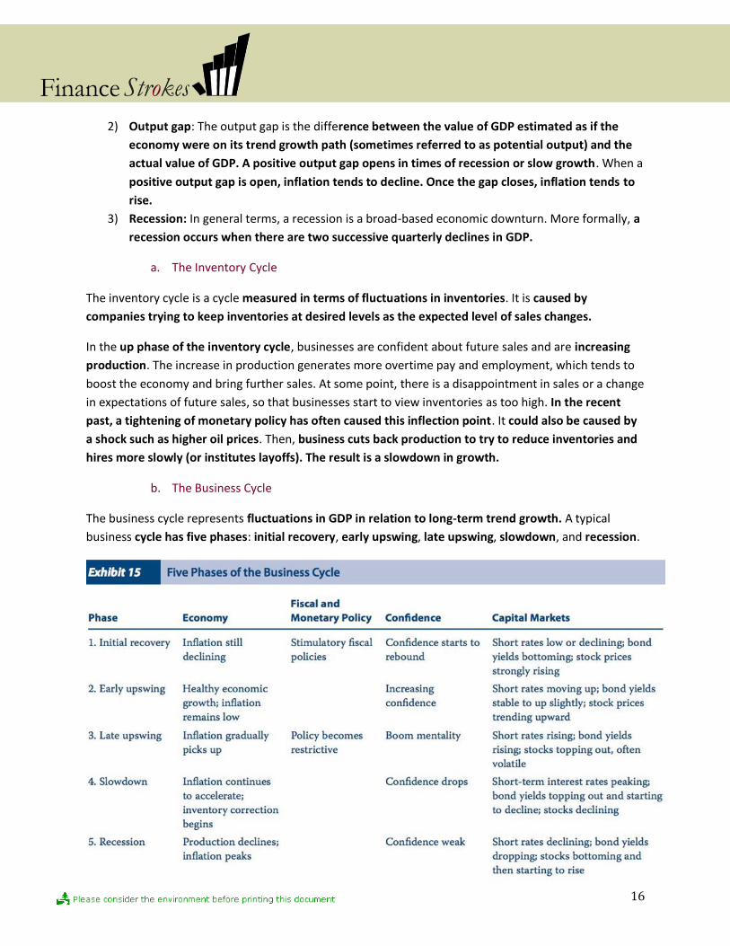
b. The Business Cycle

The business cycle represents fluctuations in GDP in relation to long-term trend growth. A typical

business cycle has five phases: initial recovery, early upswing, late upswing, slowdown, and recession.

17

Trends that have affected the business cycle from the 1990s through the late 2000s include the

growing importance of China in world markets, the aging of populations, and the deregulation of

markets. Events such as a petroleum or financial crisis can abruptly take the economy to the next phase

of the business cycle or intensify the current phase.

The yield spread between the 10-year T-bond rate and the 3-month T-bill rate has been found

internationally to be a predictor of future growth in output. The observed tendency is for the yield

spread to narrow or become negative prior to recessions. Another way of saying the same thing is

that the yield curve tends to flatten or become inverted prior to a recession.

Effects that may explain a declining yield spread include the following:

1) Future short-term rates are expected to fall, and/or

2) Investors’ required premium for holding long-term bonds rather than short-term bonds has

fallen. At least, the link between an expected decline in short-term rates from expected lower

loan demand and declining output growth is economically somewhat intuitive.

When the yield spread is expected to narrow (the yield curve is moving toward inversion), long-duration

bonds should outperform short-duration bonds. On the other hand, a widening yield spread (for

example, an inverted yield curve moving to an upward-sloping yield curve) favors short-duration bonds.

c. Inflation and Deflation in the Business Cycle

Inflation is linked to the business cycle, tending to rise in the late stages of a business cycle and to

decline during recessions and the early stages of recovery. However, the analyst also needs to note any

long-term trends in inflation in formulating capital market expectations.

Central bank orthodoxy for dealing with inflation rests on three principles:

1) Central banks’ policy-making decisions must be independent of political influence. If political

pressure is brought to bear on central banks, they may be too loose in their monetary policy and

allow inflation to gradually accelerate.

2) Central banks should have an inflation target, both as a discipline for themselves and as a signal

to the markets of their intentions. An inflation target also serves to anchor market expectations.

3) Central banks should use monetary policy (primarily interest rates) to control the economy

and prevent it from either overheating or languishing in a recession for too long.

Deflation is a threat to the economy for two main reasons.

1) It tends to undermine debt-financed investments.

2) Deflation undermines the power of central banks. In a deflation, interest rates fall to levels

close to zero. When interest rates are already very low, the central bank has less leeway to

stimulate the economy by lowering interest rates.

In today’s economies, prolonged deflation is not really likely. In the now distant past, prolonged deflation

was caused by the limited money supply provided by the gold standard currency system. With

governments able to expand the money supply to any desired degree, there is really no reason for

deflation to last long. Nevertheless, even today, weak periods within the business cycle can still bring

short periods of deflation, even if the upswing phases produce inflation.

18

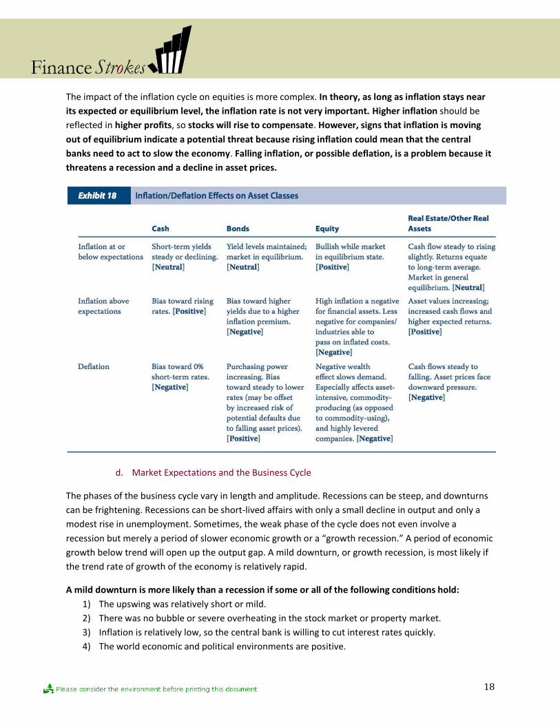
The impact of the inflation cycle on equities is more complex. In theory, as long as inflation stays near

its expected or equilibrium level, the inflation rate is not very important. Higher inflation should be

reflected in higher profits, so stocks will rise to compensate. However, signs that inflation is moving

out of equilibrium indicate a potential threat because rising inflation could mean that the central

banks need to act to slow the economy. Falling inflation, or possible deflation, is a problem because it

threatens a recession and a decline in asset prices.

d. Market Expectations and the Business Cycle

The phases of the business cycle vary in length and amplitude. Recessions can be steep, and downturns

can be frightening. Recessions can be short-lived affairs with only a small decline in output and only a

modest rise in unemployment. Sometimes, the weak phase of the cycle does not even involve a

recession but merely a period of slower economic growth or a “growth recession.” A period of economic

growth below trend will open up the output gap. A mild downturn, or growth recession, is most likely if

the trend rate of growth of the economy is relatively rapid.

A mild downturn is more likely than a recession if some or all of the following conditions hold:

1) The upswing was relatively short or mild.

2) There was no bubble or severe overheating in the stock market or property market.

3) Inflation is relatively low, so the central bank is willing to cut interest rates quickly.

4) The world economic and political environments are positive.

19

e. Evaluating Factors that Affect the Business Cycle

For the purposes of setting capital market expectations, we need to focus business cycle analysis on four

areas:

1) Consumers;

2) Business;

3) Foreign trade;

4) Government activity, both monetary policy (concerning interest rates and the money supply)

and fiscal policy (concerning taxation and governmental spending). There are three motivations

for government to intervene in the cycle.

a. Both the government and monetary authorities may try to control the cycle to mitigate

severe recessions and also, on occasion, to moderate economic booms.

b. The central bank monetary authorities often have an inflation target and they will

consciously try to stimulate or constrain the economy to help meet it.

c. Because incumbent politicians prefer to hold elections during economic upswings, they

may try to influence fiscal and/or monetary policy to achieve this end.

i. Taking the Pulse of Consumers

The principal sources of data on consumer spending are retail sales, miscellaneous store sales data,

and consumer consumption data. Like most data, consumer spending can be erratic from month to

month and can be affected by unusual weather or holidays (such as New Year celebrations). By far the

most important factor affecting consumption is consumer income after tax, which depends on wage

settlements, inflation, tax changes, and employment growth. Employment growth is often closely

watched because data are usually available on a very timely basis.

ii. Taking the Pulse of Business

Data on business investment and spending on inventories reveal recent business activity. As already

mentioned, both tend to be relatively volatile so that it is not uncommon for business investment to fall

by 10–20 percent or more during a recession and to increase by a similar amount during strong

economic upswings. Data for inventories need careful interpretation. A report of rising inventories may

mean that businesses are very confident of sales and are spending on inventories ahead of expected

sales. This would normally be the case in the early stages of an inventory cycle upswing and is bullish

for economic growth. But at the late stage of the inventory cycle, a rise in inventories may be

involuntary because sales are lower than expected. Such news would be negative. Some of the most

useful data on business are surveys. A particularly useful one is the purchasing managers index (PMI).

iii. Monetary Policy

Monetary policy is sometimes used as a mechanism for intervention in the business cycle. For

example, monetary policymakers may switch to stimulative measures (increasing money supply growth

and/or lowering short- term interest rates) when the economy is weak and restrictive measures

(decreasing money supply growth and/or raising short-term interest rates) when the economy is in

danger of overheating. If unemployment is relatively high and there is spare capacity, then a rate of

20

GDP growth higher than the trend rate will be tolerated for a while. This scenario is typical of the

recovery and early upswing phases of the business cycle. In the late upswing phase, the economy is

threatening to overheat and monetary authorities will restrict money supply to slow growth. If they

get it wrong and a recession emerges, then they will cut rates sharply to restore growth. Finally, if a

major financial crisis threatens the financial system, they will also cut rates sharply and flood the

economy with liquidity.

The key variables watched by monetary authorities are as follows:

The pace of economic growth;

The amount of excess capacity still available (if any);

The level of unemployment; and

The rate of inflation.

Central banks often see their role as smoothing out the growth rate of the economy to keep it as near as

possible to its long-term sustainable trend rate—in effect, neither too hot nor too cold. Lower rates

encourage more borrowing by consumers and businesses. Lower interest rates also usually result in

higher bond and stock prices. These in turn encourage consumers to spend more and encourage

businesses to invest more. From an international trade perspective, lower interest rates usually lower

the exchange rate and therefore stimulate exports. The effect of a cut in interest rates also depends on

the absolute level of interest rates, not just the direction of change.

What matters is not whether interest rates have most recently been moved up or down but where they

stand in relation to their average or “neutral” level. It is common to think of this “neutral” level as a

point of interest rate equilibrium within the economy. The concept of the neutral level of interest rates

is an important one, though in reality, it is impossible to identify precisely. Conceptually, the argument

is that a neutral level of short-term interest rates should include a component to cover inflation and a

real rate of return component.

The Taylor Rule

This rule links a central bank’s target short-term interest rate to the rate of growth of the economy

and inflation to assess the central bank’s stance and to predict changes:

𝑹𝒐𝒑𝒕𝒊𝒎𝒂𝒍 = 𝑹𝒏𝒆𝒖𝒕𝒓𝒂𝒍 + [𝟎. 𝟓 × (𝑮𝑫𝑷𝒈𝒇𝒐𝒓𝒆𝒄𝒂𝒔𝒕 − 𝑮𝑫𝑷𝒈𝒕𝒓𝒆𝒏𝒅) + 𝟎. 𝟓 × (𝑰𝒇𝒐𝒓𝒆𝒄𝒂𝒔𝒕 − 𝑰𝒕𝒂𝒓𝒈𝒆𝒕)]

Where,

𝑅𝑜𝑝𝑡𝑖𝑚𝑎𝑙 = the target for the short term interest rate

𝑅𝑛𝑒𝑢𝑡𝑟𝑎𝑙 = the short-term interest rate that would be targeted if GDP growth were on trend and inflation on target 𝐺𝐷𝑃𝑔𝑓𝑜𝑟𝑒𝑐𝑎𝑠𝑡 = the GDP forecast growth rate

𝐺𝐷𝑃𝑔𝑡𝑟𝑒𝑛𝑑 = the observed GDP trend growth rate 𝐼𝑓𝑜𝑟𝑒𝑐𝑎𝑠𝑡 = the forecast inflation rate

𝐼𝑡𝑎𝑟𝑔𝑒𝑡 =the target inflation rate

21

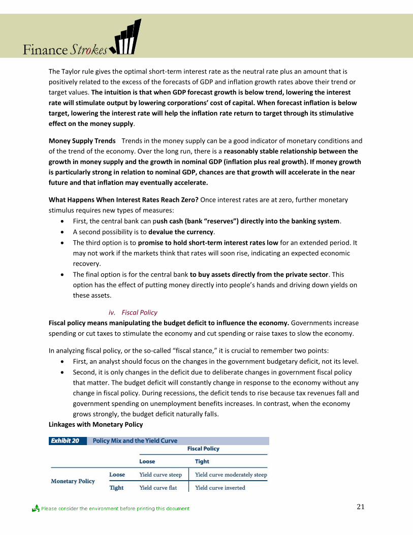
The Taylor rule gives the optimal short-term interest rate as the neutral rate plus an amount that is

positively related to the excess of the forecasts of GDP and inflation growth rates above their trend or

target values. The intuition is that when GDP forecast growth is below trend, lowering the interest

rate will stimulate output by lowering corporations’ cost of capital. When forecast inflation is below

target, lowering the interest rate will help the inflation rate return to target through its stimulative

effect on the money supply.

Money Supply Trends Trends in the money supply can be a good indicator of monetary conditions and

of the trend of the economy. Over the long run, there is a reasonably stable relationship between the

growth in money supply and the growth in nominal GDP (inflation plus real growth). If money growth

is particularly strong in relation to nominal GDP, chances are that growth will accelerate in the near

future and that inflation may eventually accelerate.

What Happens When Interest Rates Reach Zero? Once interest rates are at zero, further monetary

stimulus requires new types of measures:

First, the central bank can push cash (bank “reserves”) directly into the banking system.

A second possibility is to devalue the currency.

The third option is to promise to hold short-term interest rates low for an extended period. It

may not work if the markets think that rates will soon rise, indicating an expected economic

recovery.

The final option is for the central bank to buy assets directly from the private sector. This

option has the effect of putting money directly into people’s hands and driving down yields on

these assets.

iv. Fiscal Policy

Fiscal policy means manipulating the budget deficit to influence the economy. Governments increase

spending or cut taxes to stimulate the economy and cut spending or raise taxes to slow the economy.

In analyzing fiscal policy, or the so-called “fiscal stance,” it is crucial to remember two points:

First, an analyst should focus on the changes in the government budgetary deficit, not its level.

Second, it is only changes in the deficit due to deliberate changes in government fiscal policy

that matter. The budget deficit will constantly change in response to the economy without any

change in fiscal policy. During recessions, the deficit tends to rise because tax revenues fall and

government spending on unemployment benefits increases. In contrast, when the economy

grows strongly, the budget deficit naturally falls.

Linkages with Monetary Policy

22

2- Economic Growth trends

The economic growth trend is the long-term growth path of GDP. The long-term growth path reflects

the average growth rate around which the economy cycles. Business cycles take the economy through

an alternating sequence of slow and fast growth, often including recessions and economic booms.

Economists are concerned with a variety of trends besides the economic growth trend, because that

trend is determined by other economic trends, such as population growth and demographics, business

investment and productivity, government structural policies, inflation/deflation, and the health of

banking/lending processes.

a. Consumer Impacts: Consumption and Demand

Consumers spend more in response to perceived increases in their wealth due to a “wealth effect,”

overall consumer consumption is quite stable over the business cycle. Milton Friedman (1957)

developed an explanation for this stability in his permanent income hypothesis. The permanent income

hypothesis asserts that consumers’ spending behavior is largely determined by their long-run income

expectations. Thus, consumer trends are usually stable or even countercyclical over a business cycle.

When incomes rise the most (during the cyclical expansion phase), spending increases less than income

rises. When incomes fall as an economy’s growth slows or declines, consumption falls only a fraction

and usually only for a relatively short period of time.

b. A Decomposition of GDP Growth and Its Use in Forecasting

The simplest way to analyze an economy’s aggregate trend growth/ trend growth in GDP is to split it

into:

Growth from changes in employment /labor inputs:

o growth in the size of the potential labor force

o growth in the actual labor force participation rate

Growth from changes in labor productivity:

o Productivity increases come from investment in equipment or new machines/capital

inputs

o Growth in total factor productivity (TFP growth), known also as technical progress and

resulting from increased efficiency in using capital inputs.

The potential sources of TFP growth include technological shocks and shifts in government policies. In

historical analyses, TFP is often taken simply as a “residual”— that is, output growth that is not

accounted for by the other factors.

23

c. Government Structural Policies

Government structural policies refer to government policies that affect the limits of economic growth

and incentives within the private sector. Government policies affect economic growth trends in

profound ways.

The following are elements of a pro-growth government structural policy:

1) Fiscal policy is sound. Even though investors prefer to see governments hold the budget deficit

close to zero over the long term, fiscal policy is sometimes used to influence the business cycle

and can play a useful role. For example, decreasing a budget surplus (or increasing a budget

deficit) may be a justifiable economic stimulusduring a recession. But countries that regularly

run large deficits tend to have one or more of three potential problems.

First, a government budget deficit often brings a current account deficit (the so-called

“twin deficits” problem), which means that the country must borrow abroad.

Eventually, when the level of foreign debt becomes too high, that borrowing must be

scaled back. This usually requires a large and potentially destabilizing devaluation of

the currency.

Second, if the deficit is not financed by borrowing, it will ultimately be financed by

printing money, which means higher inflation.

Third, the financing of the deficit takes resources away from private sector

investment, and private sector investment is usually more productive for the country

as a whole. It is for all these reasons

2) The public sector intrudes minimally on the private sector. According to economic theory, a

completely free competitive market would probably supply too little in the way of public

goods, such as national defense, and too much in the way of goods with negative externalities,

such as goods whose manufacture pollutes the environment. However, the thrust of economic

theory is that the marketplace usually provides the right incentives to individuals and businesses

and leads to an efficient allocation of scarce resources. The most damaging regulations for

business tend to be labor market rules (e.g., restricting hiring and firing) because such

regulations tend to raise the structural level of unemployment (the level of unemployment

resulting from scarcity of a factor of production); however, such regulations are also the most

difficult to lift.

2) Competition within the private sector is encouraged. Competition is important for trend

growth because it drives companies to be more efficient and therefore boosts productivity

growth. Sound structure includes: the reduction of trade tariffs and barriers, recent advances in

networking technologies, openness to foreign investment. However, note that competition

makes it more difficult for companies to earn high returns on capital and thus can work

against high stock market valuations.

3) Infrastructure and human capital development are supported. Projects supporting these goals

may be in partnership with the private sector. Building health and education infrastructure has

important economic benefits.

24

4) Tax policies are sound. Governments provide a range of goods, including defense, schools,

hospitals, and the legal system. They also engage in a certain amount of redistribution of income

directly, through pensions and welfare programs. According to economic theory, taxes distort

economic activity by reducing the equilibrium quantities of goods and services exchanged. A

decrease in total societal income and efficiency is the cost of redistributing wealth to the least

well-off. As a result, investors often look with skepticism on governments that impose high

overall tax burdens. Sound tax policy involves simple, transparent, and rarely altered tax rates;

low marginal tax rates; and a very broad tax base.

3- Exogenous Shocks

Exogenous shocks are events from outside the economic system that affect its course. Over time,

trends in an economy are likely to stay relatively constant. As such, they should already be discounted in

market expectations and prices. Exogenous shocks may have short-lived effects or drive changes in

trends. They are typically not built into prices or at most are only partially anticipated.

Most shifts in trends are likely to come from shifts in government policies, which is why

investors closely watch both specific measures and the overall direction of government policy.

The biggest impact occurs when there is new government or a major institutional shift.

The creation and assimilation of new products, markets, and technologies provide a positive,

longer-term impact on economic trends. Too often, analysts focus on shorter-term benefits,

under-appreciating the evolving nature of the technologies and the scope of their effects. These

gains show up in TFP growth.

Shocks cannot be forecast in general. But there are two types of economic shock that

periodically affect the world economy and often involve a degree of contagion, as problems in

one country spread to another:

1) Oil shocks are important because a sharp rise in the price of oil reduces consumer

purchasing power and also threatens higher inflation. A sudden rise in prices affects

consumers’ income and reduces spending. Inflation rates also rise, though here the

effect is ambiguous. Although inflation moves up initially, the contractionary effect

of higher oil prices restricts employment and opens up an output gap so that, after a

period, inflation slows to below the level where it otherwise might have been. There

have also been episodes of declining oil prices, these tend to have the effect of

extending the economic upswing because they contribute to lower inflation. Low oil

prices and low inflation boost economic growth that can contribute to overheating

2) Financial shocks, which can arise for a variety of reasons, threaten bank lending and

therefore economic growth. Periodic financial crises affect growth rates either

directly through bank lending or indirectly through their effect on investor

confidence. Banks are always potentially vulnerable after a major decline in asset

prices, particularly property prices, financial crises are potentially more dangerous

in a low interest rate environment.

25

4- International Interactions

In general, the dependence of any particular country on international interactions is a function of its

relative size and its degree of specialization. Increasing globalization of trade, capital flows, and direct

investment means that practically all countries are increasingly affected by international interactions.

a. Macroeconomic Linkages

Countries’ economies are directly affected by changes in the foreign demand for their exports. This is

one way that the business cycle in one country can affect that in others. But there are other

international linkages (other than trade) at work, such as those resulting from cross-border direct

business investment.

b. Interest Rate/Exchange Rate Linkages

One of the linkages of most concern to investors involves interest rates and exchange rates.

Sometimes, short-term interest rates are affected by developments in other countries because one

central bank pursues a formal or informal exchange rate link with another currency. Some

governments unilaterally peg their currencies firmly orloosely to one of the major currencies, usually

the U.S. dollar or the euro. The countries that follow this strategy find two benefits:

First, domestic business has some reassurance that exchange rates are not going to fluctuate

wildly.

Second, by pegging the exchange rate, a “pegged” country often hopes to control inflation. If a

country is following such an exchange rate policy, then the level of interest rates will depend

on overall market confidence in the peg. A high degree of confidence in the exchange rate peg

means the interest rate differential can converge to near zero. But if the markets see the peg

policy as unsustainable, then investors will demand a substantial interest differential. If a

country is known to be linking its currency to another, then bond yields of the weaker currency

are nearly always higher.

Exchange rates can be over or undervalued, requiring an offset from bond yields, for a number of

reasons, such as government action on short-term interest rates. For example, the Exchange Rate

Mechanism was maintained as long as it was by using high short-term interest rates to limit speculation

against currencies. Misvaluation can also happen when bond yields reflect a particularly strong

economy.

Nominal bond yields vary between countries according to those countries’ different inflation outlooks

and other factors. It is sometimes thought that real bond yields ought to be similar in different

countries because international capital flows will equalize them. However, movements in exchange

rates to under- or over- valued levels can compensate for different real bond yields. Although real

yields can and often do vary among countries, they tend to move together. The key factor linking bond

yields (especially real bond yields) is world supply and demand for capital or the perceptions of supply

and demand.

26

c. Emerging Markets

There are some special considerations in setting capital market expectations for emerging countries.

i. Essential Differences between Emerging and Major Economies

Emerging countries are engaged in a catch-up process. As a result, they need higher rates of

investment than developed countries in physical capital and infrastructure and in human capital. But

many emerging countries have inadequate domestic savings and therefore rely heavily on foreign

capital. Unfortunately, managing the consequent foreign debt often creates periodic crises, dealing a

major blow to investors in emerging stocks and bonds.

Four factors usually associated with emerging market economies are as follows:

1) Emerging market economies require high rates of investment, which is usually in short supply

within the emerging economy itself. This situation creates a reliance on foreign capital. Areas of

needed investment usually include both physical assets (capital equipment and infrastructure)

and human capital (education and skills building).

2) Emerging economies typically have volatile political and social situations. Leaders usually

acquire and maintain power using force and other less- than-democratic means. The social

environment is usually strained by the fact that a large portion of the population possesses few

assets, has little formal education, and is unable to generate income to feed/support family and

neighbors.

3) To alleviate the first two factors above, organizations such as the IMF and World Bank provide

conduits for external sources of investment and a means to push for structural reforms—

political, social, educational, pro- growth, etc. The “conditions” usually prescribed by these

institutions are often felt to be draconian.

4) Emerging countries typically have economies that are relatively small and undiversified. Those

emerging economies that are dependent on oil imports are especially vulnerable in periods of

rising energy prices and can become dependent on ongoing capital inflows.

ii. Country Risk Analysis Techniques

Investors in emerging bonds focus on the risk of the country being unable to service its debt. Investors

in stocks need to assess the growth prospects of emerging countries as well as their vulnerability to

surprises. A common approach is to use a checklist of various economic and financial ratios and a

series of qualitative questions:

1) How sound is fiscal and monetary policy? If there is one single ratio that is most watched in all

emerging market analysis, it is the ratio of the fiscal deficit to GDP . A persistent ratio above 4

percent is regarded with concern. The range of 2–4 percent is acceptable but still damaging.

Countries with ratios of 2 percent or less are doing well. If the fiscal deficit is large for a

sustained period, the government is likely to build up significant debt. In developing countries,

governments usually borrow in the short term from domestic lenders in local currency and from

overseas in foreign currency. For a developing country, the level of debt that would be

considered too high is generally lower than for developed countries. Countries with a ratio of

debt of more than about 70–80 percent of GDP are extremely vulnerable.

27

2) What are the economic growth prospects for the economy? Annual growth rates of less than 4

percent generally mean that the country is catching up with the industrial countries slowly, if at

all. It also means that, given some population growth, per capita income is growing very slowly

or even falling, which is likely to bring political stresses. One of the best indicators of the

structural health of an economy is the Economic Freedom Index, which consists of a range of

indicators of the freedoms enjoyed by the private sector, including tax rates, tariff rates, and the

cost of setting up companies. The index has been found to have a broad positive correlation

with economic growth.

3) Is the currency competitive, and are the external accounts under control? Managing the

currency has proven to be one of the most difficult areas for governments. If the exchange rate

swings from heavily undervalued to seriously overvalued, there are negative effects on business

confidence and investment. Moreover, if the currency is overvalued for a prolonged period, the

country is likely to be borrowing too much, creating a large current account deficit and a

growing external debt. The size of the current account deficit is a key measure of

competitiveness and the sustainability of the external accounts. Any country with a deficit

persistently greater than 4 percent of GDP is probably uncompetitive to somedegree. Current

account deficits need to be financed. If the deficits are financed through debt, servicing the debt

may become difficult. A combination of currency depreciation and economic slowdown will

likely follow. The slowdown will also usually cut the current account deficit by reducing imports.

Note, however, that a small current account deficit on the order of 1–3 percent of GDP is

probably sustainable, provided that the economy is growing. A current account deficit is also

more sustainable to the extent that it is financed through foreign direct investment rather than

debt, because foreign direct investment creates productive assets.

4) Is external debt under control? External debt means foreign currency debt owed to foreigners

by both the government and the private sector. It is perfectly sensible for countries to borrow

overseas because such borrowing serves to augment domestic savings. The ratio of foreign debt

to GDP is one of the best measures. Above 50 percent is dangerous territory, while 25–50

percent is the ambiguous area. Another important ratio is debt to current account receipts. A

reading above 200 percent for this ratio puts the country into the danger zone, while a reading

below 100 percent does not.

5) Is liquidity plentiful? By liquidity, we mean foreign exchange reserves in relation to trade flows

and short-term debt. Traditionally, reserves were judged adequate when they were equal in

value to three months’ worth of imports. An important ratio is reserves divided by short-term

debt. A safe level is over 200 percent, while a risky level is under 100 percent.

6) Is the political situation supportive of the required policies? If the economy of the country is

healthy, with fast growth, rapid policy liberalization, low debt, and high reserves, then the

answer to this question matters less. Poor political leadership is unlikely to create a crisis.

However, if the economic indicators and policy are flashing warning signals, the key issue

becomes whether the government will implement the necessary adjustment policies.

28

5- Economic Forecasting

Some of the disciplines and approaches that the analyst can apply to economic forecasting include:

a. Econometric Modeling

Econometrics is the application of quantitative modeling and analysis grounded in economic theory to

the analysis of economic data. Whereas generic data analysis can involve variables of all descriptions,

econometric analysis focuses on economic variables, using economic theory to model their

relationships.

A model is created of the economy based on variables suggested by economic theory. Optimization

using historical data is used to estimate the parameters of the equations. The estimated system of

equations is used to forecast the future values of economic variables, with the forecaster supplying

values for the exogenous variables.

A very simple model is presented in the following series of equations:

1) GDP growth = function of (Consumer spending growth and investment growth)

2) Consumer spending growth = function of (Consumer income growth lagged one period and

Interest rate*)

3) Investment growth = function of (GDP growth lagged one period and Interest rate*)

4) Consumer income growth lagged one period = Consumer spending growth lagged one period

Here, the asterisk (*) denotes an exogenous variable. So, with this four-equation model estimated on

past data and with the actual data for the variables lagged one period, together with the modeler’s

exogenous forecasts for the interest rate, the modelwill solve for GDP growth in time in the current

period. Note that the final equation asserting that consumer income growth is always identical to

consumer spending growth assumes a static relationship between these two variables.

Econometric models are widely regarded as very useful for simulating the effects of changes in certain

variables. The great merit of the econometric approach, however, is that it constrains the forecaster to a

certain degree of consistency and also challenges the modeler to reassess prior views based on what the

model concludes.

Econometric models have several limitations. First, econometric models require the user to find

adequate measures for the real-world activities and relationships to be modeled, and these measures

may not be available. Variables may also be measured with error. Relationships among the variables

may change over time because of changes in the structure of the economy; as a result, the econometric

model of the economy may be misspecified. In practice, model-based forecasts rarely forecast

recessions well, although they have a better record in anticipating upturns.

b. Economic Indicators

Economic indicators are economic statistics provided by government and established private

organizations that contain information on an economy’s recent past activity or its current or future

29

position in the business cycle. Lagging economic indicators and coincident indicators are indicators of

recent past and current economic activity, respectively. A leading economic indicator (LEI) is a variable

that varies with the business cycle but at a fairly consistent time interval before a turn in the business

cycle. Most analysts’ greatest interest is leading indicators because they may provide information about

upcoming changes in economic activity, inflation, interest rates, and security prices.

Analysts may use both individual LEIs and composite LEIs, reflecting a collection of economic data

releases that are combined to give an overall reading. Composite LEIs combine these releases using

weights based on an analysis of their forecasting usefulness in past cycles. They can also be combined in

a so-called diffusion index, which measures how many indicators are pointing up and how many down.

We review a selection of LEIs, both individual and composite, by geographic region:

Worldwide

OECD Composite Leading Indicators (CLI): A Total OECD Composite Leading Indicator is published, as

well as indices for the 23 member countries and for seven regions:

Europe

Eurozone Harmonized Index of Consumer Prices (HICP)

German Industrial Production

The German IFO Business Survey

The French Monthly Business Survey

Asia Pacific

The Tankan Survey of the Bank of Japan

China Industrial Production

The Chinese currency (called the renminbi or yuan) on a purchasing power parity basis

South America

Brazil Industrial Production

30

North America

The Conference Board’s Index of Leading Economic Indicators

c. Checklist Approach

Checklist assessments are straightforward but time-consuming because they require looking at the

widest possible range of data. The data may then be extrapolated into forecasts via objective statistical

methods, such as time-series analysis, or via more subjective or judgmental means. An analyst may then

assess whether the measures are in an equilibrium state or nearer to an extreme reading.

31

The subjectivity of the checklist approach is perhaps its main weakness. The check- list’s strength is its

flexibility. It allows the forecaster to take changes in the structure of the economy into account quickly

by changing the variables or the weights assigned to variables within the analysis.

32

d. Economic Forecasting Approaches: Summary of Strengths and Weaknesses

6- Using Economic Information in Forecasting Asset Class Returns

Principal asset classes that are moved by different economic variables include:

a. Cash and Equivalents

Cash managers make money through selection of the maturity of the paper in their portfolio or, if

permitted by investment policy, by taking credit risk. Longer maturities and lower credit ratings

reward the extra risk with higher expected returns. Managers lengthen or shorten maturities

according to their expectations of where interest rates will go next. Normally, longer-maturity paper

will pay a higher interest rate than shorter-maturity paper, even if overnight interest rates are expected

to remain the same, because the risk of loss is greater for the longer-term paper if this expectation is not

fulfilled. If further rises in rates are expected over time, then 6- and 12-month paper should offer even

higher rates than shorter-term paper.

33

The overnight interest rate is targeted by the central bank and will normally vary only slightly from the

target set.

At any given time, the yield curve of interest rates of a particular security reflects the market’s

expectations of rates over that period. The money manager is trying to be ahead of others in correctly

forecasting those levels. In practice, this means forecasting both the behavior of the economy and the

reaction of the central bank to that behavior. It also means understanding what the markets currently

anticipate and distinguishing between future data surprises and what is already factored into

expectations.

b. Nominal Default-Free Bonds

Nominal default-free bonds are conventional bonds that have no (or minimal) default risk.

Conventional government bonds of developed countries are the best example. Thus, our focus is on the

government yield curve. One way to think of the yield on a government bond is that it reflects the

expected future short-term Treasury bill yields over the same horizon. Another approach, which is

more useful for longer-term bonds, is to break down the yield into at least two components:

First, the so-called real bond yield is determined by the growth rate of GDP and the supply and

demand for capital.

Second, yields are affected by forecast inflation over the investment period. For default-risk-

free bonds, the credit spread or default risk premium is zero. Investors may thus assess whether

bonds are cheap or expensive according to their view on whether the markets are too optimistic

or too pessimistic based on real yields and inflation.

For investors buying and selling long-term bonds over a shorter time period, the emphasis is on how

bond yields will respond to developments in the business cycle and changes in short-term interest rates.

News of stronger economic growth usually makes bond yields rise (prices fall) because it implies greater

demand for capital and perhaps higher inflation too. Changes in short-term rates have less predictable

effects on bond yields. More often than not, a rise in short-term rates will lead to a rise in longer-term

bond yields. However, a rise in rates will sometimes be expected to slow the economy, and bond yields

could fall as a result. If bond markets expect that central banks will exactly achieve their inflation

objectives, then bond yields should not change on inflation expectations but nevertheless could go up

and down according to changes in short rates (with higher short rates making bonds less attractive in

relative terms).

As bond investors look toward the long-term picture, they must carefully assess the future effects of

inflation, which erodes the future purchasing power of the yields earned on their fixed-income

investments.

c. Defaultable Debt

Defaultable debt is debt with some meaningful amount of credit risk—in particular, most corporate

debt. For corporate debt, such as certificates of deposit and bonds, the spread over Treasuries

represents at least in part the market’s perception of default risk. Individual securities move in

34

response to particular corporate circumstances, but the market as a whole responds primarily to

changes in short-term rates and changes in the business cycle. During a business cycle, spreads tend to

rise during a recession because companies are under stress from both weak business conditions and,

typically, higher interest rates. Sometimes, borrowing from banks or in the commercial paper market

becomes more difficult too, so that companies can be severely squeezed. Default rates typically rise

during recessions. Investors demand higher rates to pay for the uncertainties and possible surprises,

such as fraud. In contrast, during periods of strong economic growth, spreads narrow as fears of

default decline.

d. Emerging Market Bonds

Emerging market debt refers here to the sovereign debt of nondeveloped countries. So far, we have

considered only government issues and regarded them as virtually risk-free from a credit point of view.

Emerging market bonds, as an asset class, are different in that the country is borrowing in a foreign

currency. The government therefore cannot simply inflate its way out of a problem in servicing the

debt, and so the risk of default is correspondingly higher. Much of country risk analysis comes down to

predicting policy moves and therefore often hinges on politics—that is, whether a government has the

power to follow the necessary policies to stabilize the economy. Emerging market bonds are usually

analyzed by developed market investors in terms of their spread over domestic Treasuries compared to

similarly rated domestic corporate debt.

e. Inflation-Indexed Bonds

Many governments now issue bonds linked to inflation, so in principle, we can directly observe the

market’s forecast of inflation by comparing the yield of these indexed bonds with the yield on

similarly dated conventional bonds. These provide a fixed coupon (the real portion) plus an adjustment

equal to the change in consumer prices. In principle, indexed bonds are the perfect risk-free asset

because, unlike conventional bonds, they entail no risk from unexpected inflation. However, the yield on

indexed bonds still changes over time, and in practice it varies with three economic factors:

First, the yield goes up and down with the real economy and particularly with the level of

short-term interest rates. If real yields generally are high because the economy is strong, then

real yields on TIPS and ILGs will be higher.

Second, yields fall if inflation accelerates because these securities are more attractive when

inflation is volatile. In other words, their value in hedging against inflation risk is higher.

Finally, as with all assets, the yield can vary according to institutional supply and demand. In practice, tax effects and the limited size of the market may also distort the real yield; thus, investors usually find it worthwhile to forecast all three components.

35

f. Common Shares

To relate economic analysis to common equity valuation, it is useful to think of economic factors:

First, in the way that they affect company earnings and,

Second, in the way that they affect interest rates, bond yields, and liquidity.

The two views combined provide a forecast for the equity markets and can lead to new investor ideas

and trading activity.

i. Economic Factors Affecting Earnings

In the long term, the trend growth in aggregate company earnings is mainly determined by the trend

rate of growth of the economy. The trend rate of growth of an economy is dependent on labor force

growth, the level of investment, and the rate of labor productivity growth. Variations in growth rates

among countries are usually due to past overinvestment, government overregulation or political

instability, or the bursting of a major asset price bubble.

Over the shorter term, the share of profits in GDP varies with the business cycle and is influenced by a

variety of factors, including final sales, wages, capacity utilization, and interest rates.

ii. The P/E Ratio and the Business Cycle

The price-to-earnings ratio of a stock market is the price that the market is willing to pay for the

earnings of that market. During the business cycle, the P/E ratio tends to be high and rising when

earnings are expected to rise. Conversely, P/Es are likely to be low and falling if the outlook for earnings

worsens. Nevertheless, P/ Es of cyclical companies may be above their own historical means during

economic downturns as investors anticipate a sharp future earnings recovery when the economy turns

up (a phenomenon known as the Molodovsky effect).

P/E ratios vary over longer periods too. In general, they are lower for an economy stuck on a slower

growth path. High inflation rates tend to depress P/E ratios. Inflation can distort the economic meaning

of reported earnings, leading investors to value a given amount of reported earnings less during

inflationary periods, which tends to lower observed P/Es during those periods. Consequently,

comparisons of current P/E with past average P/E that do not control for differences in inflation rates

may be suspect.

iii. Emerging Market Equities

Empirical evidence points to ex post equity risk premiums for emerging markets that are on average

higher and more volatile than those in developed markets. In addition to evaluating linkages, the

analyst needs to do considerable country and often sector-specific research to appraise the prospects

for equity investments in a particular emerging country.

g. Real Estate

Ling and Naranjo (1997, 1998) identify growth in consumption, real interest rates, the term structure of

interest rates, and unexpected inflation as systematic determinants of real estate returns. Interest

36

rates are linked with a number of factors that affect the supply and demand for real estate, such as

construction financing costs and the costs of mortgage financing. In general, lower interest rates are

net positive for real estate valuation, resulting in lower capitalization rates.

h. Currencies

The exchange rate between two countries reflects the balance of buyers and sellers. One major reason

for buying and selling foreign currencies is to facilitate trade in goods and services (exports and imports).

If a country begins to import more, the currency will tend to depreciate (all else being equal). Hence,

considerable attention is usuallypaid to determining a competitive exchange rate at which the trade

balance—or, more broadly, the current account balance (which includes services and transfers)—is zero.

Governments and central banks are often concerned with maintaining a competitive exchange rate and

may try to do so by buying or selling foreign currencies or by raising or lowering interest rates.

However, trade is only one motive for purchases and sales of foreign currency and it has become

relatively less important. The other motive is international flows of capital. Companies wishing to invest

in a country are likely to be buyers of the currency as they bring in capital to build assets. Strong

domestic economic growth and an opening of new industries to foreign ownership are two possible

drivers of a rise in foreign direct investment that will likely push up a currency too. The liberalization of

capital flows and the increasing trend toward global diversification mean that there may also be inflows

to buy local stocks, bonds, or short-term instruments, including deposits. These flows can be volatile and

may quickly reverse. The foreign direct investment is likely to be more stable.

Portfolio flows may be influenced by the growth of the economy or by domestic interest rates. When

interest rates are high, inflows are likely to be higher and the currency value rises. Conversely, falling

interest rates often weaken a currency. However, the link between interest rates and the currency

sometimes works the other way. This is because investors may see higher interest rates as slowing the

economy. If a currency departs from the level that equilibrates trade for a long time, the resulting deficits

or surpluses may eventually become too large for capital flows to finance. Among the major currencies,

there are often prolonged over- and undervaluations around a long-term equilibrium level. For this

reason, many governments in emerging countries use some combination of capital controls and currency

management to try to keep the currency competitive. This approach tends to lead to stability for

extended periods punctuated by periodic sudden, large movements.

i. Approaches to Forecasting Exchange Rates

There are four broad approaches to forecasting exchange rates, and most forecasters probably use a

combination of them all.

i. Purchasing Power Parity (need to know the exact calculation method refer to

practice problems or CFA 2 notes)

Purchasing power parity (PPP) asserts that movements in an exchange rate should offset any

difference in the inflation rates between two countries. PPP reflects the idea that exchange rates

should find a level that keeps different countries broadly competitive with each other.

37

PPP in broad terms does seem to be useful in the long run. Furthermore, governments and central banks

take PPP very seriously in their approach to exchange rates because periods of under- or overvaluation

of a currency may lead to sudden exchange rate instability or be destabilizing for business.

However, with the huge rise in capital flows over the last three decades, exchange rates can depart from

PPP levels for long periods of time. PPP is often not a useful guide to the direction of exchange rates in

the short or even medium run (up to three years or so). There are also times when factors other than

PPP dominate exchange rate movements. This usually happens when a large current account deficit is

opening up and the markets question whether a growing deficit can be financed. Markets then focus on

what level of the currency is needed to correct the deficit.

ii. Relative Economic Strength

The relative economic strength forecasting approach focuses on investment flows rather than trade

flows. It suggests that a strong pace of economic growth in a country creates attractive investment

opportunities, increasing the demand for the country’s currency and causing it to appreciate.

Sometimes, demand comes from a higher short-term deposit rate in that country combined with an

expectation that the currency will stay the same or appreciate. More recently, the focus has been on the

pace of economic growth and the existence of attractive investment opportunities in general.

When interest rates are relatively high in a country, capital moves into that country and, as a result, the

currency strengthens. Even if investors begin to see the exchange rate as overvalued in some long-term

sense, they may still be content if they feel the extra yield compensates for that overvaluation. However,

once the exchange rate reaches an excessive level, they will question whether the high yield is enough to

justify the likely exchange rate depreciation.

What is the role of short rates? There is little question that short-term interest rates can influence

exchange rates but primarily over a short-term time horizon. The level of short-term interest rates

influences the extent to which speculators are willing to bet against a currency. If interest rates in a

particular country are especially high, speculators are less likely to short that currency because that

currency will probably strengthen as a result of the higher interest rates.

It can be helpful to combine the PPP and relative strength approaches. The relative strength approach

indicates the response to news on the economy but does not tell us anything about the level of

exchange rates. The PPP approach indicates what level of the exchange rate can be regarded as a

long-term equilibrium. By combining the two, we can generate a more complete theory.

iii. Capital Flows

The capital flows forecasting approach focuses on expected capital flows, particularly long-term flows

such as equity investment and foreign direct investment (FDI). Inflows of FDI into a country increase

the demand for the country’s currency, all else being equal.

Note that long-term capital flows may have the effect of reversing the usual relationship between

short-term interest rates and the currency. This is explained by the fact that a cut in short-term rates

would be expected to boost economic growth and the stock markets, thereby making long-term

38

investments more attractive. In this environment, central banks face a dilemma. Whereas they might

want to raise interest rates to respond to a weak currency that is threatening to stimulate the

economy too much and boost inflation, the effect may actually be to push the currency lower. Hence,

the effectiveness of monetary policy is much reduced.

iv. Savings–Investment Imbalances

The savings–investment imbalances forecasting approach explains currency movements in terms of

the effects of domestic savings–investment imbalances on the exchange rate. Although it is not easy to

use for forecasting, this approach can sometimes help with understanding why currencies depart from

equilibrium for long periods. It starts from the fact that the current account deficit of a country is the

sum of its government deficit and private sector deficit.

Suppose that an economy suddenly begins to expand rapidly, driven by a new government budget deficit

or bullish entrepreneurs. If domestic savings do not change, there will be excess demand for capital as

investment tries to exceed savings. The only way that investment can exceed savings in reality is for

foreign savings to be used, since the accounts have to balance. But this solution requires a deficit on the

current account of the balance of payments. So, where does this deficit on the current account come

from? Some of it may arise simply because imports are strong due to the buoyant economy or because

exports are weak as companies focus on the domestic market. But if that is not enough, the exchange

rate needs to rise. If capital flows are attracted to the country, either due to high interest rates or due to

attractive expected returns on investments, then the exchange rate will indeed rise as needed.

Because trade takes time to adjust, the exchange rate will frequently depart far from generally accepted

equilibrium rates for prolonged periods, typically two to four years. Eventually, the rising currency will

widen the current account deficit sufficiently and the domestic currency may start to decline. Of course, it

needs to stay reasonably strong as long as domestic investment exceeds savings.

If the economy becomes weak enough at this point and domestic investments no longer exceed domestic

savings, then the currency will also weaken. To return to a current account surplus, the exchange rate

may need to drop to a level well below its equilibrium rate. Hence, there is a risk that the currency could

swing sharply to an undervalued position.

j. Government Intervention

Economists and the markets have been skeptical about whether governments really can control

exchange rates with market intervention alone because of three factors:

First, the total value of foreign exchange trading, in excess of US$1 trillion daily, is large relative

to the total foreign exchange reserves of the major central banks combined.

Second, many people believe that market prices are determined by fundamentals and that

government authorities are just another player.

Third, experience with trying to control foreign exchange trends is not encouraging in the

absence of capital controls. Unless governments are prepared to move interest rates and other

policies, they cannot expect to succeed.