Embed Size (px)
Citation preview

METHODOLOGY OF HOMOGENEOUS AND
NON-HOMOGENEOUS MARKOV CHAINS FOR
MODELLING BRIDGE ELEMENT DETERIORATION
Final Report
to
Michigan Department of Transportation
Center for Advanced Bridge Engineering
Civil and Environmental Engineering Department
Wayne State University
By
GONGKANG FU
&
DINESH DEVARAJ
August 2008

DISCLAIMER
The content of this report reflects the views of the authors, who are responsible for the
facts and accuracy of the information presented herein. This document is disseminated
under the sponsorship of the Michigan Department of Transportation in the interest of
information exchange. The Michigan Department of Transportation assumes no liability
for the content of this report or its use thereof.

ACKNOWLEDGEMENTS
This project was conducted under the direction of Messrs. Robert Kelley and David
Juntunen. Their constant support and effort are gratefully appreciated. Without that this
project would not have been successfully completed. A number of graduate students of
the Center for Advanced Bridge Engineering at Wayne State University, including but
not limited to Messrs. Pang-jo Chun, Yizhou Zhuang, and Tapan Bhatt, assisted in a
variety of tasks of this project. Their contribution is acknowledged with gratitude.

TABLE OF CONTENTS
Chapter 1 Introduction……………………………………………………………1
1.1 Background and Organisation of Report……………………………1
1.2 Literature Review………………………………………………….....2
1.2.1 Review………………………………………………………....3
1.2.2 Summary……………………………………………………....9
Chapter 2 State of the Practice in Bridge Management System………………11
Chapter 3 Markov Chain………………………………………………………. 22
3.1 Markov Chain as A Stochastic Process……………………………. 22
3.2 Transition Probability in Markov Chain………………………….. 23
3.3 Homogeneous Markov Chain………………………………………. 28
3.4 Non-Homogeneous Markov Chain…………………………………. 28
3.5 Properties of Transition Probabilities……………………………… 29
3.6 “Do-Nothing” Transition Probabilities……………………………... 30
Chapter 4 An Arithmetic Method For Estimating Transition Probabilities… 33
Chapter 5 Pontis Method of Transition Probability Estimation……………… 37
5.1 Estimation of Transition Probabilities for One Time Step Using
Inspection Data………………………………………………………. 38
5.2 Combination of Estimated Transition Probability Matrices for
Different Time Steps…………………………………………………. 49
Chapter 6 Limitations of the Pontis Approach…………………………………. 55
6.1 Non-invertible [XX] matrix…………………………………………... 55
6.2 Negative Transition Probabilities……………………………………. 56

6.3 Possible Non-zero p13, p14, p15,p24, p25, p35, p21, p31, p32, p41, p42,
p43, p51, p52, p53, and/or p54 values……………………………….. 60
Chapter 7 Proposed Method of Transition Probability Estimation…………… 62
7.1 Optimization Formulation for Estimating Transition Probabilities. 62
7.2 A Simple Illustrative Example……………………………………….. 64
7.3 An Application Example……………………………………………. 67
7.4 More Application Examples and Discussions………………………. 74
Chapter 8 Summary and Conclusions…………………………………………… 80
References
Appendix

1
CHAPTER 1 INTRODUCTION
1.1 Background and Organisation of Report
Bridge management is an important activity of transportation agencies in the US
and in many other countries. A critical aspect of bridge management is to reliably predict
the deterioration of bridge structures, so that appropriate or optimal actions can be
selected to reduce or minimize the deterioration rate and maximize the effect of spending
for replacement or maintenance, repair, and rehabilitation (MR&R). In the US, Pontis is
the most popular bridge management system used among the state transportation
agencies. Its deterioration model uses the Markov Chain, with a statistical regression to
estimate the required transition probabilities. This is the core part of deterioration
prediction in Pontis.
This report focuses on the Markov Chain model used in Pontis, which is vital to
the understanding and implementation of the Pontis software. Emphasis has been made
on the limitations of Pontis methodology, and establishing a new method for transition
probability estimation. This is because predicting deterioration is the basis for decision-
making with respect to MR&R. The next portion of this chapter presents a literature
review on the subject of estimating transition probability matrix using Markov Chain for
modeling deterioration in civil engineering facilities, such as bridges, pavements, and
waste water systems.
This report consists of seven additional chapters. Chapter 2 will present the results
of a survey regarding the application of bridge management in the US and Canadian

2
transportation agencies. In Chapter 3, the basic concept of Markov Chain will be
introduced in a simplified way with an emphasis on application. Simple examples are
included to facilitate easy understanding. That chapter covers both homogeneous and
non-homogeneous Markov chains for background information and comparison. Pontis
uses a homogenous Markov chain model.
Chapter 4 presents a simple arithmetic algorithm for quickly estimating the
transition probabilities, which will aid in understanding the concept of “transition”.
However, this approach is not appropriate or proposed for routine application for
predicting deterioration, since it lacks a capability to statistically cover possible random
variation in condition data. This is to be seen in the examples included in this report.
Chapter 5 discusses the approach used in Pontis for estimating the transition probability
matrix. Chapter 6 highlights the issues associated with the Pontis approach for updating
the transition probabilities, especially for Michigan. Chapter 7 presents the proposed
method for transition probability estimation, based on the concept of non-homogenous
Markov Chain. Here the proposed method will be compared with the existing Pontis
approach, and the arithmetic method. Chapter 8 offers a summary for this research effort
and the conclusions reached.
1.2 Literature Review:
The Markov Chain has been the most commonly used methodology to predict the
deterioration of bridge structures and elements. The core of Markov Chain is the
transition probability matrix because it is the basis for deterioration prediction. Thus,
realistically estimating this matrix is critical. To understand the state of the art in the

3
estimation of the transition probability matrix in Markov Chain a literature review was
performed particularly for transportation application facilities such as bridges and
pavements. As a result three relevant papers are summarized below. There were also
other papers found to be helpful, which are included in the reference list of this report.
1.2.1 Review
(1) José J. Ortiz-García; Seósamh B. Costello, and Martin S. Snaith (2006),
“Derivation of Transition Probability Matrices for Pavement Deterioration Modeling,”
Journal of Transportation Engineering, Vol. 132, No. 2, Feb 1, 2006
In this paper pavement deterioration modeling in general is divided into two broad
groups, the deterministic- and the probabilistic-based approaches. Mathematical models
are used to predict the deterioration (or the future condition state) as a fixed value in the
deterministic approach, and as a probability for a particular condition in the probabilistic
approach. It was pointed out in the paper that out of these two broadly classified models,
the probabilistic modeling using Markov prediction is more frequently used.
This research effort attempted to compare methods for estimating the transition
probabilities. Three candidate methods were tested on six sets of artificial data
specifically synthesized for this purpose.
The first method directly uses historical condition data of the system for selecting
the optimal transition probabilities available. The second utilizes a regression curve
obtained from the original data as a criterion for estimation, and the third assumes that the
distributions of condition are available to assist in the process. More details are to be

4
presented and discussed below about these different methods for estimating the transition
probabilities.
The six artificial data sets were generated using the same basic concepts for
condition rating. The system’s condition is defined on a scale ranging from 0 to 100, with
0 for intact condition and 100 for complete disintegration. The score range is further
divided into 10 intervals each having a width of 10 and defined as a condition state. The
midpoints of these intervals are taken as the names of the condition states, namely 95, 85,
75, 65, 55, 45, 35, 25, 15, and 5. So data cjt is the condition State j at time t. Each data set
is to simulate annually collected conditions for 30 sites of a network over a 20-year
period. Data Set 1 represents an S-shaped deterioration curve typical of the trend
associated with either cracking or raveling progression in pavements. Data Set 2
represents a deterioration curve where the rate of progression starts slowly but increases
with age. Data Sets 3 to 5 represent deterioration curves where the rate of progression
starts fast but decreases with age, with each of the data sets representing a different rate
of deterioration. Finally, Data Set 6 represents a completely random rate of progression.
Method A – This method is to find the transition probabilities by minimizing the
sum of the squared differences between each of the data points and the average condition
calculated from the distributions of condition. The objective of the estimation is to
minimize
Objective Function 2
( )jt
t j
Z c y t = − ∑∑ (1.1)
where cjt is the condition data for State j at time t as defined earlier, and ( )y t is the
condition at time t weighted by the distribution vector using the estimated transition
probabilities

5
( )y t = a(t).c (1.2)
where c = (95, 85, 75, 65, 55, 45, 35, 25, 15, 5) is the vector indicating the midpoints of
the condition intervals between 90 and 100, 80 and 90, 70 and 80, 60 and 70, 50 and 60,
40 and 50, 30 and 40, 20 and 30, 10 and 20, 0 and 10, respectively. In other words, these
midpoints can be viewed as the nominal values for the 10 condition level in the Markov
Chain. a(t) is the probability distribution at time t.
a(t) 1 2 3 10{ ( ), ( ), ( ),......., ( )}Ta t a t a t a t= (1.3)
where ai(t) for i = 1, 2, ……, 10 are the probabilities for the respective states at time t,
( )y t = 95a1(t) + 85a2(t) + 75a3(t) +65a4(t) +55a5(t) +45a6(t) +35a7(t) +25a8(t) +15a9(t) +
5a10(t) . Vector a(t) depends on the estimated transition probability matrix P, which is
selected to minimize the objective function Z in Equation (1.1)
Method B - In this method, a regression is performed first using the collected data
cjt. This results in y(t) as a relation between the condition (defined as 95, 85, 75, 65, ….,
and 5 as above) and time t. The objective function Z for this case is defined to be
minimized as follows:
Objective Function 2
( ) ( )t
Z y t y t = − ∑ (1.4)
The objective of this method is to minimize this function as the squared distance between
the regression curve y(t) and the transition-probability-matrix-fitted curve y (t).
Method C - In this method, the raw data are presented in the form of distributions.
The objective function Z is calculated as
6
Objective Function 2
'( ) ( )i i
t i
Z a t a t = − ∑∑ (1.5)
where ( )i
a t has been defined in Equation (1.3), and ' ( )i
a t for i =1, 2, 3, 4,…….,10 are
probabilities for condition i at time t obtained using raw data cjt.
For all the test data sets, Method C yielded distributions closer to the “observed”
distributions (i.e., distributions based on the synthesized inspection data) than Methods A
and B. The distributions determined from Method C were also comparable, in many cases
almost identical, to the “observed” ones. It is thus concluded that Method C is most
appropriate for estimating the transition probability matrix.
Note that Method C directly used the observed distributions ' ( )i
a t for i=1, 2, 3, …,
10 in the optimization requirement “Z” defined in Equation (1.5), and Methods B and C
does not. Therefore, the above conclusion is not surprising. Furthermore using ' ( )i
a t as a
criterion for estimating the transition probabilities is a realistic and thus reasonable
approach, because it is important to determine the transition probabilities to be able to
reliably predict future conditions of the system.
(2) G. Morcous (2006), “Performance Prediction of Bridge Deck Systems
Using Markov Chains,” Journal of Performance of Constructed Facilities, Vol. 20, No. 2,
May 1, 2006.
In this work it is stated that the stochastic Markov-Chain models are used in
current bridge management systems for performance prediction because of their ability to
capture the time dependence in predicting bridge deterioration. The required life-cycle
cost assessment of bridges is based on these predictions. It is a decision making process

7
based on the total cost for the bridge over its lifetime depending on the need for
maintenance or demolition. The various costs involved in bridge management are
construction cost, maintenance cost, demolition cost, and the user cost (indirect costs
caused by detour, accidents, etc).
Bridge management systems such as Pontis and BRIDGIT adopt the Markov-
Chain model for performance prediction of components, systems, and networks. The
criterion used in this research for transition probability estimation is to minimize
Objective Function Z = ( ) ( )t
C t E t−∑
subject to 0 1ijp≤ ≤ , 1, 2,..,i j n= (1.6)
1ij
j
p =∑ i = 1, 2, …., n
where ( )C t is the system condition rating at time t based on regression. This function
describes a statistical relation between the condition and time t, obtained by regression
analysis using data from inspection of the bridges. ( )E t is the expected rating at time t
based on the Markov Chain using the estimated transition probabilities. This method
appears to be similar to Method B in (Ortiz-Gorcia et.al 2006) discussed earlier.
(3) Hyeon-Shik Baik; Hyung Seok (David) Jeong; and Dulcy M. Abraham
(2006) “Estimating Transition Probabilities in Markov Chain-Based Deterioration
Models for Management of Wastewater Systems,” Journal of Water Resources Planning
and Management, Vol. 132, No. 1, January 1, 2006.
The so called ordered probit model was used in this work to estimate the
transition probabilities for a Markov Chain based deterioration model for wastewater

8
systems. It uses a non-homogeneous Markov Chain for this purpose. The condition
assessment data set used to evaluate the developed method was obtained from the City of
San Diego. It was concluded that the ordered probit model approach seemed to provide a
theoretically and statistically more robust model as compared to the nonlinear
optimization-based approach for the estimation of transition probabilities. In the non-
linear optimization based approach, the transition probabilities are estimated by
minimizing the following objective function,
Objective Function Z = ( ) ( , )t n
Y t E n−∑∑ P
subject to 0 1ijp≤ ≤ , 1, 2 , . . , 5i j = (1.7)
1ij
j
p =∑ 1, 2,..,5i =
where t is the system’s age, n is the number of transitions and P is the transition
probability matrix. Y (t) is the average condition rating at t based on a regression
analysis:
0 . 9 4 9 0 . 0 4 4( ) tY t e
− += (1.8)
using the condition data. E(n,P) is the predicted condition rating after n transitions based
on the Markov Chain model using the estimated transition probabilities in P. This
approach appears to be also similar to that used in Equation (1.6).
It was also pointed out that, for developing accurate models using the ordered
probit model, it is necessary to have panel data that span over multiple time periods. In
order to predict more accurate and detailed deterioration patterns of wastewater systems,
9
factors such as the depth of the installation, the soil condition, the groundwater level, and
the frequency of sewage overflows should be collected and evaluated.
A major drawback that has been discussed in this paper is that, in the current
inspection practices, the information discussed here is not readily available for
wastewater systems. It is emphasized that a standardized condition rating system is
required to generate a more robust deterioration model and to evaluate the deterioration
processes of wastewater systems among different municipalities. By employing a
standardized condition rating system, current management practices and future
investment planning can be evaluated. Another problem is that, currently each
municipality uses a different rating system for its wastewater systems. These different
condition-rating systems prevent comparison of the effects of maintenance and
information sharing regarding condition assessment among municipalities.
Based on this discussion, the ordered probit model does not appear to be suitable
for current practice of bridge management, due to its higher requirement for a large
amount of data to allow modeling non-homogenous stochastic processes.
1.2.2 Summary
The literature review shows that Markov Chain is a popular and plausible tool to
model system or element deterioration and improvement. For bridge management, it
appears to be reasonable as well. In addition, the computation effort for using Markov
Chain is also affordable for bridge management, considering several to tens of thousand
bridges involved in a typical state.

10
In applying the Markov Chain model, the critical step is to estimate the transition
probability matrix based on observation data. Several approaches have been proposed for
this purpose. It seems to be agreeable that the ability to reliably predict deterioration
comparable with observed deterioration is required. On the other hand, it should be
emphasized that this requirement can only be used for the time period in which
observation or inspection data have been collected. Predictions to the future beyond this
time period cannot be evaluated until more data become available.

11
CHAPTER 2 STATE OF THE PRACTICE IN BRIDGE
MANAGEMENT SYSTEM
In this chapter the experiences of US and Canadian transportation agencies with
bridge management system is reviewed based on their response to a questionnaire. The
questionnaire developed in this project included two parts. The first one had a set of 13
questions categorized under “General Questions”. The second one was framed as
“Additional Information and Comments”. The complete questionnaire is included in the
appendix to this report. A total of thirty one agencies responded to the survey. The
details of these two categories and the agency responses are presented in this chapter.
In the “General Questions” groups, there were a total of 13 questions aimed to
understand various aspects of bridge management system application. These questions
are further categorized below for analysis. The first sub-category of questions is to gather
general information on the type of bridge management system (BMS) and on the bridge
condition data available. There are 3 questions in this sub-category as follows:
1. Which BMS does your agency use?
2. Approximately how many years of bridge condition data (inspection and/or asset
management data) does your agency have in your database?
3. What bridge condition data are used within your BMS?
Table 2.1 exhibits the responses to these questions. It shows Pontis as the most
popular system currently being used. Also more agencies (16) have data between 4 to 10
years, compared with 11 agencies with more than 10 years of data. For those agencies

12
that use Pontis, all of them use both the NBI and the CoRe formats except Florida that
uses CoRe only. Note that six US agencies using Pontis are also using data other than
NBI and CoRe.
Table 2.1: Bridge Management Systems in and Condition Data Available
States 1 2 3
Which BMS is
used ?
No. of years of bridge
condition data
Type of condition data
Alaska Pontis >10 NBI / CoRe
Alberta In-House system > 10 Other
Arizona In-House system 4 to 10 NBI / CoRe
Arkansas Pontis 1 to 3 NBI / CoRe
Colorado Pontis 4 to 10 NBI / CoRe / Other
Delaware Pontis 4 to 10 NBI / CoRe / Other
District of Columbia 4 to 10 NBI / CoRe
Florida Pontis 4 to 10 CoRe
Georgia Pontis 0 to 1 NBI / CoRe
Hawaii Pontis 4 to 10 NBI / CoRe
Illinois Pontis > 10 NBI / CoRe
Iowa In-House system (Code Sheets)
1 to 3 NBI
Kansas Pontis > 10 NBI / CoRe
Maine Pontis >10 NBI / CoRe / Other
Maryland In-House system 4 to 10 NBI / CoRe / Other
Minnesota Pontis 4 to 10 NBI / CoRe
Mississipi Pontis 4 to 10 NBI / CoRe

13
Montana Pontis > 10 NBI / CoRe
Nevada Pontis > 10 NBI / CoRe
New Mexico Pontis 4 to 10 NBI / CoRe
New York In-House system (Bridge Needs
Assessment Model) > 10 Other
Ohio In-House system >10 Other
Ontario In-House system 4 to 10 Other (element condition state)
Puerto Rico Pontis 4 to 10 NBI / CoRe
South Carolina Pontis >10 NBI / CoRe
Tennessee Pontis > 10 NBI / CoRe
Utah Pontis 1 to 3 NBI / CoRe / Other
Vermont Pontis 4 to 10 NBI / CoRe
Virginia Pontis 4 to 10 NBI / CoRe
Washington Pontis 4 to 10 NBI / Other
Wyoming Pontis 4 to 10 NBI / CoRe / Other
The second sub-category of questions was to know the practice in agency-specific
application. Such application involves element definition, development of maintenance,
rehabilitation, and repair (MR&R) policies, and cost estimation. These are questions
were used to gather relevant information:
4. If your agency is a Pontis user, have you made modifications to the AASHTO
CoRe elements, and/or have you added additional elements?

14
5. Has you agency developed bridge preservation policies, for maintenance,
rehabilitation, and repair (MR&R)?
6. What cost data do you use to determine cost parameters for projects in your
BMS?
Table 2.2: Agency Specific Application or Modification
States 4 5 6
Modifications to CoRe Elements (If Pontis user)
MRR policy developed?
Type of Cost Data
Alaska Yes No Past Bid /
Bridge Maintenance Crew
Alberta No Past Bid
Arizona No
Arkansas Yes No Past Bid
Colorado Yes No Past Bid
Delaware Yes Yes Past Bid
District of Columbia No Past Bid
Florida Yes No Past Bid
Georgia Yes No Past Bid
Hawaii No No Past Bid
Illinois Yes Yes Past Bid
Iowa
No Past Bid
Kansas Yes No Past Bid
Maine Yes Yes Past Bid
Maryland Not a Pontis user No
Minnesota Yes Yes Past Bid
Mississippi Yes No

15
Montana Yes Yes Past Bid
Nevada Yes No Default data
in Pontis
New Mexico No Yes Past Bid
New York No Past Bid
Ohio Past Bid
Ontario Yes Past Bid
Puerto Rico No No Past Bid
South Carolina Yes Yes MR&R cost -
SCDOT, Others – contract
Tennessee Yes No Past Bid
Utah Yes Yes Past bid compared with annual cost and average MRR costs
Vermont No No Past Bid
Virginia Yes Yes Past Bid
Washington Yes Yes Past Bid
Wyoming Yes No Past Bid
Table 2.2 shows that 19 out of the 23 Pontis states have modified the CoRe
definitions and 4 have not. On the other hand, only about a half (11) of them have
develop their own MR&R policies. A vast majority (26) of the 31 agencies are using bid
prices for cost estimation, only one is using the Pontis default cost values.
The next sub-category questions focused on the transition probabilities in the
Markov Chain modeling. There were three questions on how the transition probabilities
are obtained or estimated, and the satisfaction associated with it. The three questions in
this sub-category are:

16
7. Does your agency use deterioration rates based on transition probabilities?
8. If your agency is a Pontis user, are you satisfied with the resulting transition
probabilities or deterioration rates (Do you think they model the situation
realistically)?
9. How does your agency determine the transition probabilities or deterioration rates
for a bridge element?
Table 2.3 Generation and Application of Condition Transition Probabilities
States 7 8 9
Deterioration rates based on
Transition Probabilities?
Satisfied with Transition
Probabilities? (If Pontis User)
How to determine Transition Probability
or Deterioration rate?
Alaska Yes Need to evaluate Historic and Expert
Elicitation
Alberta No Historic and Expert
Elicitation
Arizona No
Arkansas Yes Yes Expert Elicitation
Colorado No Not implemented Not implemented
Delaware Yes Yes Expert Elicitation
District of Columbia
Yes Historic and Expert
Elicitation
Florida Yes Yes Expert Elicitation
Georgia
No Historic and Expert
Elicitation
Hawaii Yes Under development Expert Elicitation
Illinois Yes Yes Historic and Expert
Elicitation
Iowa No
Kansas Yes Yes Historic and Expert
Elicitation
Maine No Yes / Partially Historic

17
Maryland No No
Minnesota Yes Partially Expert Elicitation
Mississipi No
Montana Yes Yes Historic and Expert
Elicitation
Nevada As in Pontis Not yet started
using
New Mexico No Haven’t Tried Historic and Expert
Elicitation
New York No Historic Data
Ohio Historic only
Ontario Yes Expert Elicitation
Puerto Rico No
South Carolina Yes Yes / Partially Historic and Expert
Elicitation
Tennessee No Yes Historic and Expert
Elicitation
Utah Yes No Expert Elicitation
Vermont Yes Partially Historic and Expert
Elicitation
Virginia Yes Partially Expert Elicitation
Washington Historic and Expert
Elicitation
Wyoming Yes Yes Historic and Expert
Elicitation
Sixteen agencies here use deterioration rates based on the transition probabilities,
and 11 said not using. This seems to indicate that the condition transition probabilities
are considered important to the agencies. Out of the 23 Pontis states, 8 reported
satisfaction with the transition probabilities produced in Pontis, 5 said partially satisfied,
3 said not satisfied, and 5 yet to evaluate (or not responding to the question). This
distribution of response indicates a reasonable success with Pontis but also some room
for improvement as well. For estimating the transition probabilities, 13 out of the 23

18
Pontis states use historic data and elicitation, 7 use elicitation only, and the rest either did
not respond or have not reached this stage of implementation. This situation of a large
number of agencies using elicitation is perhaps because the available historic data still do
not meet the need for reliable estimation of the transition probabilities.
The last sub-category of questions in the general questions section included
miscellaneous subjects related to application and satisfaction as follows:
10. Has your agency compared your BMS with your traditional approach for bridge
management decision making?
11. Do you think your agency’s BMS fully meets your need for bridge management?
12. Please describe how your agency determines the discount rate for project cost
projection to the future.
13. How does your agency perform rulemaking and project prioritization within the
BMS?
Table 2.4 shows the responses received to these questions. Fourteen agencies out
of the 31 that responded reported experience with comparison of the BMS and
traditional approaches, 15 said not, and the rest did not respond and most likely did
not have such experience. We believe such an experience is important for the
calibration of the BMS. As to the question whether the BMS meets the agency’s
needs, 17 out of 31 said no in addition to one that did not respond to this particular
question. For comparison, 12 confirmed that the BMS does meet their needs. This
large number of negative response to the question deserves attention. One possible

19
explanation to this situation is that, as mentioned earlier, available data are not
adequate to model the behavior of the bridges and thus to help decision making.
For determining the discount rate, only very few agencies spend an effort to
estimate the rate, many agencies use the Pontis default, and a large number (17) of the
agencies do not use it, yet to determine it, or did not respond. To the last question in
this group of general questions, most (20) agencies either did not respond or reported
that rulemaking and project prioritization are not done currently. Others reported
some traditional ways of practice, including “Collaboration between main
office and field staff”, “BMS, maintenance engineers and bridge review team”,
“Rules based on bridge administrative manual”, “NBI ratings”, “Cost benefit analysis
& bridge condition index”, “Bridge Condition ratio along with engineering
judgment”, etc.
For the second group of questions for additional information and comments,
including whether the agencies are familiar with other relevant work and have
additional comments, a few agencies responded positively. We then followed up by
phone calls or e-mails to clarify and/or locate the specific information to acquire
written documentations for the specific experience. In addition, 25 out of the 31
agencies that responded answered positively to the question whether they would like
to have the results of this survey. It shows a strong interest in this research work.

20
Table 2.4: Changes Made for Prioritization
States 10 11 12 13
BMS vs
Traditional Approach Compared
Does your BMS meet
all your needs?
Discount rate methodology
How rule making and project
prioritization is performed?
Alaska No no Default used Not done
Alberta Yes No 4% based on Historic Data
Not done
Arizona Yes
Arkansas No Yes
Colorado Yes Yes Not implemented Not done
Delaware Yes Rules are written so as to be compatible with
Pontis
District of Columbia
No No Not used
Florida No No Work program
Office
Georgia No Yes Not Determined Not Determined
Hawaii Yes As in Pontis Under implementation
Illinois Yes Yes Limited by design Top down approach
Iowa No No National Inflation Index
Collaboration between main office and field staff
Kansas Yes Yes As in Pontis As in Pontis
Maine Yes No
Default used - Its thought that
Pontis is not sensitive
to this value
BMS, maintenance engineers and bridge
review team
Maryland No Yes
Minnesota Yes No As in Pontis Not done
Mississipi No No
Montana Yes No Bonding rate Rules based on
bridge administrative manual
Nevada No No
New Mexico No Yes Guessing NBI ratings
New York No No No
Ohio No No
Ontario No Yes Provincial govt.'s finance ministry
Cost benefit analysis & bridge condition
index
Puerto Rico No

21
South Carolina Yes Yes Pontis MR&R and Own inflation rate
Bridge Condition ratio along with engineering
judgment
Tennessee Yes No Yet to set up Not done
Utah Yes No Inflation Rate (4%) Concept Report ( Scope, schedule and budget is
defined)
Vermont Yes Yes Work is being done Work is being done
Virginia Yes No As in Pontis In the development
stage
Washington No Yes
Wyoming No No As in Pontis Not done

22
CHAPTER 3 MARKOV CHAIN
This chapter presents the basic framework of Markov Chain as a modeling tool
for bridge management. It summarizes the concept and defines the symbols used, with
simple examples for illustration.
3.1 Markov Chain as A Stochastic Process
The Markov Chain is a stochastic process as a mathematical model for a system
or an element that has random outcomes. These outcomes are viewed as a function of
independent variables such as a temporal or spatial factor. For example, the condition of a
bridge element is modeled in Pontis as a stochastic process with time t as the independent
variable, because the future condition cannot be predicted with certainty. A stochastic
process can be formally defined as follows.
Consider a series of discrete time points { }kt for k = 1, 2,….. and let
t kξ be a
random variable as the condition of a bridge element, which describes its state at time k
t .
The family of random variables { }t kξ k =1, 2,… is then said to form a stochastic
process. The total number of considered states, in general, may be finite or infinite. For
application in bridge management, a finite number of states is used. For example in
Pontis, up to 5 states are used to describe the condition of a bridge element, with 1 for the
best and 5 for the worst condition.

23
A Markov Chain is a stochastic process for which a future state depends only on
the immediately preceding state, not any further previous states. This Markovian property
for { }t kξ can be mathematically expressed as
{ } { }1 0 11 1, ,
n n n nt n t n t o t n t nP x x x P x xξ ξ ξ ξ ξ− −− −= = = = = =L (3.1)
Here symbol means “the given condition”, and P means the probability
and 0 1 2 1, , , ..., ,n nx x x x and x− are states of 0 1 2 1
, , . . . , ,nt t t t
ξ ξ ξ ξ−
and
.ntξ Equation (3.1) reads as “the probability of
ntξ being equal to nx given that
1, . . . ,
ntξ
− and
0tξ are equal to 1nx − ,…., and 0x is equal to the probability of
ntξ being equal to nx only if
1ntξ
−is equal to 1nx − ”. Namely, the conditions at
time tn-2, tn-3, …, t0 do not affect the condition at tn , only the condition at tn-1 does.
3.2 Transition Probability in Markov Chain
The probability P defined in Equation (3.1) is called the transition probability
which can be written in short as follows
{ }1 11n n n nt n t n x xP x x pξ ξ
− −−= = = (3.2)
This is the conditional probability of the system or element being in state nx at nt ,
given that it was in state 1nx − at 1nt − . This probability is also referred to as the one-step
transition probability, since it describes the transition of the condition between times 1nt −
and nt , over one time step or one time interval.

24
For example, p34 = 30% for a bridge element means that the probability that this
element will be in State 4 at tn, if it was in State 3 at tn-1, is 30 percent. Here tn can be, for
example, Year 1997, and tn-1 Year 1996. This also indicates that the prediction based on
the Markov Chain is probabilistic, or with uncertainty taken into account. Note also that a
30% transition probability over one year from State 3 to State 4 in reality means a very
high deterioration rate, because State 4 is considered a poor condition and State 3
significantly more acceptable.
Similarly an m-step transition probability is thus defined as
{ }n n m n m nx x t n m t n
p P x xξ ξ+ + += = = (3.3)
Here (n + m)-n = m steps indicating the time difference between tn+m and tn.. Each step
here can be defined as a day, a month, a year, 2 years, 10 years, etc., depending on the
system and its states of interest. For bridge management, Pontis uses a year as a typical
time step. Namely the transition probability matrices for bridge elements are implicitly
for 1-year periods.
In Pontis, a total of 5 condition states are used to describe the condition of bridge
elements. Initially at time t, the system may be in any one of these states. Pontis uses
{ }1 2 5, , ....,T
X x x x= to express the probability distribution for an element at the
“before” time or at the last inspection. Superscript “ T ” here means transpose (to a
column vector). For example, using the MODT Pontis data for Element 107 of bridge
01200001000B030 in Environment 1 and inspected in 1997, this distribution is expressed
as { }1 2 3 4 5, , , ,T
X x x x x x= = {0, 0, 0, 100, 0}T. It indicates that Element 107 has 0% in

25
State 1, State 2, State 3, 100% in State 4, and 0% in State 5. This means that Element 107
of this bridge is entirely in State 4.
Pontis also uses { }1 2 5, ,...,T
Y y y y= to express the probability distribution for
the system or the element at the “after” time or at the later inspection. For the same
Element 107 above in Environment 1 but inspected in 2001, this distribution is
{ }1 2 3 4 5, , , ,T
Y y y y y y= = {0, 0, 0, 82.3, 17.7}T. It indicates that Element 107 still has
0% in State 1, State 2, State 3, but 82.3% in State 4, and 17.7% in State 5. Here tn is 2001
as the later inspection time, and tn-4 is 1997 as the previous inspection time. Namely over
4 years, part (17.7%) of the bridge element has deteriorated from State 4 to State 5, which
is the worst state in the Pontis condition rating system.
Figure 3.1: Example Infomaker Screen For Probability Distribution For Element 107
In Environment 1
26
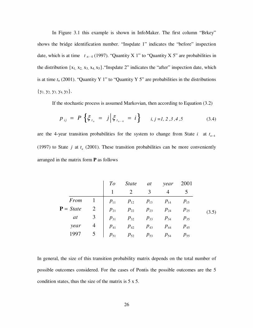
In Figure 3.1 this example is shown in InfoMaker. The first column “Brkey”
shows the bridge identification number. “Inspdate 1” indicates the “before” inspection
date, which is at time t n - 4 (1997). “Quantity X 1” to “Quantity X 5” are probabilities in
the distribution {x1, x2, x3, x4, x5}.“Inspdate 2” indicates the “after” inspection date, which
is at time tn (2001). “Quantity Y 1” to “Quantity Y 5” are probabilities in the distributions
{y1, y2, y3, y4, y5}.
If the stochastic process is assumed Markovian, then according to Equation (3.2)
{ }4n ni j t tp P j iξ ξ
−= = = i, j =1, 2 ,3 ,4 ,5 (3.4)
are the 4-year transition probabilities for the system to change from State i at 4nt −
(1997) to State j at nt (2001). These transition probabilities can be more conveniently
arranged in the matrix form P as follows
11 12 13 14 15
21 22 23 24 25
31 32 33 34 35
41 42 43 44 45
51 52 53 54 55
2001
1 2 3 4 5
1
2
3
4
1997 5
To State at year
From p p p p p
State p p p p p
at p p p p p
year p p p p p
p p p p p
=P (3.5)
In general, the size of this transition probability matrix depends on the total number of
possible outcomes considered. For the cases of Pontis the possible outcomes are the 5
condition states, thus the size of the matrix is 5 x 5.
27
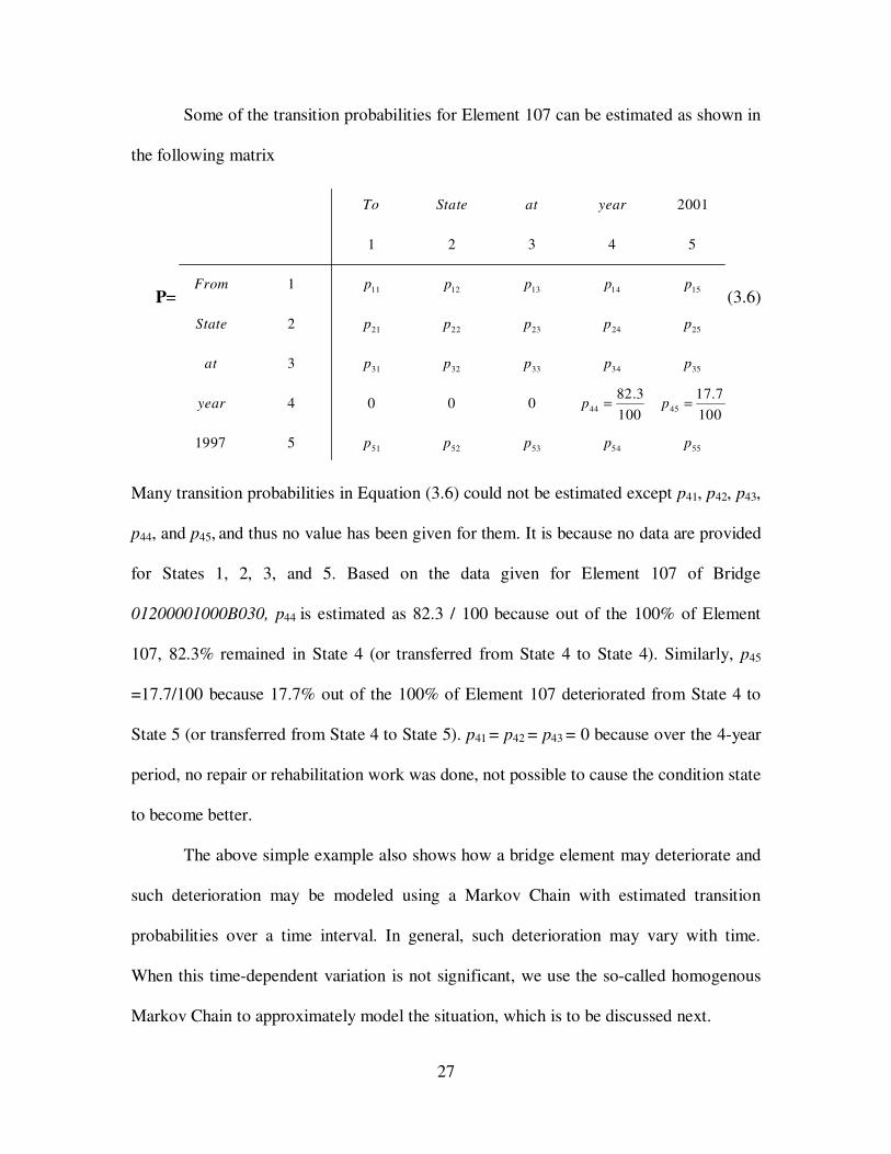
Some of the transition probabilities for Element 107 can be estimated as shown in
the following matrix
P=11 12 13 14 15
21 22 23 24 25
31 32 33 34 35
44 45
51 52 53 54 55
2001
1 2 3 4 5
1
2
3
82.3 17.74 0 0 0
100 100
1997 5
To State at year
From p p p p p
State p p p p p
at p p p p p
year p p
p p p p p
= =
(3.6)
Many transition probabilities in Equation (3.6) could not be estimated except p41, p42, p43,
p44, and p45, and thus no value has been given for them. It is because no data are provided
for States 1, 2, 3, and 5. Based on the data given for Element 107 of Bridge
01200001000B030, p44 is estimated as 82.3 / 100 because out of the 100% of Element
107, 82.3% remained in State 4 (or transferred from State 4 to State 4). Similarly, p45
=17.7/100 because 17.7% out of the 100% of Element 107 deteriorated from State 4 to
State 5 (or transferred from State 4 to State 5). p41 = p42 = p43 = 0 because over the 4-year
period, no repair or rehabilitation work was done, not possible to cause the condition state
to become better.
The above simple example also shows how a bridge element may deteriorate and
such deterioration may be modeled using a Markov Chain with estimated transition
probabilities over a time interval. In general, such deterioration may vary with time.
When this time-dependent variation is not significant, we use the so-called homogenous
Markov Chain to approximately model the situation, which is to be discussed next.

28
3.3 Homogeneous Markov Chain
A Markov Chain is called homogeneous if its transition probabilities pij defined in
Equations (3.1) to (3.3) are constant or independent of time. That means, for example, for
the same length of 2 years as a time step, the deterioration follows the same pattern no
matter when it started (i.e., no matter in which year the transition started):
{ } { }2 2k k n nt t t t
P j i P j iξ ξ ξ ξ− −
= = = = = (3.7)
for n ≠ k. Note that Pontis uses (or assumes) homogenous Markov Chains for all bridge
elements. Namely, it uses all inspection data to estimate one transition probability matrix
for one element in one environment, no matter when the inspections were done as long as
the same amount of time or approximately same amount of time has elapsed between two
inspections. Then this matrix is used in predicting or projecting future condition in the
probability sense for the same environment. This assumption for homogenous
deterioration is actually questionable because the environment condition for an element
does vary with time, especially when a long time period is concerned, such as the typical
life span of bridge.
3.4 Non-Homogeneous Markov Chain
By the name, the non-homogeneous Mark Chain model does not assume a
homogeneous behavior of the stochastic process. In other words, the transition
probability matrix P is not a constant but a function of time. Time here can be the
absolute calendar time, age, or both. Age can be viewed as a relative measure of time,
independent from the absolute time. For bridge management application, we consider the
age of the bridge element in this report. Including the absolute time represents a further

29
more general treatment of the subject. An example appropriate for such a treatment is a
scenario of special climate in a certain year that significantly alters the mechanism of
bridge element deterioration, such as a very warm winter that accelerates steel corrosion.
Since bridge elements have relatively long lives in tens to hundreds of years, an
individual year of such abnormal condition may still have limited or little influence on
deterioration and can be “averaged” out in modeling. Therefore, we include only age as
the factor to account for non-homogeneity.
3.5 Properties of Transition Probabilities
It also should be noted that pij defined in Equations (3.1) to (3.3) must satisfy the
following conditions,
1 , 2 , . . . , 5
1i j
j
p=
=∑ for all i , (3.8)
0i j
p ≥ for all i and j
Equation (3.8) means that 1) each row of the transition probability matrix adds to 1 and
2) all probabilities are non-negative. They are valid because pij is a non-negative
probability of transition from condition State i to State j, and from a State i the condition
can only become 1, 2, 3, 4, or 5. Thus the total probability (i.e., the sum) of all these
possibilities has to be 1. For example, Equation (3.6) shows the transition probabilities
for Element 107 from State 4 in Row 4, for a time period of 4 years. The sum of these pij
in that row is 1.0, because the total probability for Element 107 to transfer from State 4 to
all these states is 1.0.

30
3.6 “Do-Nothing” Transition Probabilities
Note that the matrix in Equation (3.5) in Pontis appears as a matrix for “Do-
nothing” mixed with other transition probability matrices for other MR&R options. One
example is shown in Figure 3.2. The five rows of pij for one-year marked as “Do-nothing”
are shown as:
P =
97.56 2.44 0.00 0.00 0.00
0.00 95.79 4.21 0.00 0.00
0.00 0.00 73.95 26.05 0.00
0.00 0.00 0.00 91.29 8.71
0.00 0.00 0.00 0.00 1.00
(3.9)
By comparison, one can see that this matrix being the transition probabilities for “Do-
nothing” for one-year is taken out from the other transition probabilities for other
different MR&R options. It should be noted that for searching for the optimal MR&R
strategy, an elicitation is needed for the last transition probability (p55 here for this
example) (AASHTO Pontis Manual).
Figure 3.2: An Example Pontis Screen of Transition Probabilities

31
Further note that in InfoMaker, the transition probabilities in Equation (3.5) is
shown as a vector 11 22 33 44 55{ , , , , }Tp p p p p for convenience. An example screen of this is
shown in Figure 3.3. As seen the probabilities in the vector are 94.8305, 98.6094,
99.1111, 100.00, 0. Note that Pontis has a 1.0 for p55 because an element already in State
5 will never change its state if no maintenance work is done to it. Actually, other pij’s do
not need to be shown, as seen in Figure 3.3 because the transition probability matrix is set
to have p13 = p14 = p15 = p21 = p24 = p25 = p31 = p32 = p35 = p41 = p42 = p43 = p51 =
p52 = p53 = p54 = 0 . This means that 1) transition can only occur between two consecutive
states (or no transition skipping a state can take place) and 2) improvement in condition
state is impossible under the “do-nothing” assumption. The second assertion is based on
an assumption of deterioration if nothing such as repair or rehab is done. Thus the
controlling or independent items in the matrix are those on the diagonal (i.e., p11, p22, p33,
p44, and p55), and p12, p23, p34, and p45 can be obtained using p11, p22, p33, and p44 according
to Equation (3.8), namely
12 11
23 22
34 33
45 44
1
1
1
1
p p
p p
p p
p p
= −
= −
= −
= −
(3.10)

32
Figure 3.3: An Example InfoMaker Screen of Transition Probabilities in A Vector

33
CHAPTER 4 AN ARITHMETIC METHOD FOR
ESTIMATING TRANSITION PROBABILITIES
As seen above, the transition probability matrix is an important component in the
Markov Chain model. Therefore, the criticality of reliably estimating the transition
probabilities cannot be over-emphasized. This chapter presents a simple algorithm for
quickly estimating the transition probabilities. It should be emphasized that this
estimation approach suffers from lack of a statistical basis. On the other hand, its simple
structure offers a quick estimation and understanding of the transition nature.
This simple method uses the observed condition change data over a period of time
and thereby estimates the transition probabilities. The estimation is done by creating a
transition probability matrix that can produce exactly the observed condition changes.
To illustrate the arithmetic method, let us consider an example for Element 12
(Concrete Deck – Bare in Environment 3, in square meters) for all MDOT bridges with
an inspection interval of 2 years. The condition state distributions for these bridges are
given in Table 4.1.
Table 4.1 Condition State Distributions for Element 12 in Environment 3 for
MDOT
{(0)
X } (0)
1x (0)
2x (0)
3x (0)
4x (0)
5x
in square meters 24896 34104. 15800 10300 5200
{(1)
Y } (1)
1y (1)
2y (1)
3y (1)
4y (1)
5y
in square meters 17399 34801 17200 13200 7700

34
This table indicates that for these bridges at the beginning of the 2-year period, 24896 sq.m
of the bare concrete deck was in State 1, 34104 in State 2, 15800 in State 3, 10300 in State
4, and 5200 in State 5. Two years later, the same concrete bare decks now have 17399 in
State 1, 34801 in State 2, 17200 in State 3, 13200 in State 4 and 7700 in State 5. Note that
{ (0)X } and { (1)
Y } here are given in physical quantity unit (square meters), note that this
can also be represented by percentage. These two ways of presentation actually are
equivalent with a difference of multiplicative factor. All the physical quantities can be
transferred to percentage or probability by dividing each of the 5 components of the two
vectors in Table 4.1 by the total quantity. Since the total quantity
(0) (0) (0) (0) (0) (1) (1) (1) (1) (1)
1 2 3 4 5 1 2 3 4 5x x x x x y y y y y+ + + + = + + + + is 90300 sq.m, dividing {X(0)
}
and { Y(1)
} in Table 4.1 by 90300 will give the vectors in percentage or probability.
By comparison of {X(0)
} and { Y(1)
} in Table 4.1, it is seen that 17399 sq.m of
the concrete decks remained in State 1 after 2 years of service. In other words, 7497 sq.m
(= 24896 - 17399) of the 24896 sq.m deteriorated to State 2. Out of the 34104 sq.m of bare
decks that were in State 2, 27304 sq.m [= 34801 - (24896 - 17399)] stayed in State 2 and
6800 sq.m (= 34104 - 27304) became State 3. Out of 15800 sq.m, in State 3, 10400 sq.m [=
17200 - (34104 - 27304)] stayed in State 3 and 5400 sq.m (= 15800 - 10400) moved to
State 4. Out of 10300 sq.m, in State 4, 7800 sq.m [= 13200 - (15800 - 10400)] stayed in
State 4 and 2500 sq.m (= 10300 - 7800) moved to State 5. Finally, 5200 sq.m [= 7700 -
(10300 - 7800)] out of the 5200 sq.m, which was in State 5, stayed in State 5 with 2500
sq.m (= 7700 - 5200) coming from State 4. This analysis is also documented in the last row
of Table 4.2. For convenience of review, Table 4.1 is duplicated in Table 4.2.

35
Table 4.2 An Example of Estimating Transition Probabilities
(0)X
(0)
1x (0)
2x (0)
3x (0)
4x (0)
5x
In square meters 24896 34104 15800 10300 5200 (1)
Y (1)
1y (1)
2y (1)
3y (1)
4y (1)
5y
In square meters 17399 34801 17200 13200 7700
Quantity that stayed in same
state
17399 34801 – (24896 - 17399) = 27304
17200 – (34104 -27304) =10400
13200 – (15800-10400) = 7800
7700 – (10300 - 7800) =5200
Accordingly, the transition probability { }2n ni j t t
p P j iξ ξ−
= = = for
this element (within the MDOT bridges) to change from State i at 2nt − to State j at
nt can
be estimated as follows using the results of Table 4.2
P = 11 12 13 14 15
21 22 23 24 25
31 32 33 34 35
41 42 43 44
2
1 2 3 4 5
17399 24896 173991 0 0 0
24896 24896
27304 34104 273042 0 0 0
34104 34104
10400 15800 104000 3 0 0 0
15800 15800
74 0 0 0
State at year
State p p p p p
at p p p p p
year p p p p p
p p p p
−= = = = =
−= = = = =
−= = = = =
= = = = 45
51 52 53 54 55
800 10300 7800
10300 10300
52005 0 0 0 0
5200
p
p p p p p
−=
= = = = =
(4.1a)
and thus
11 12 13 14 15
21 22 23 24 25
31 32 33 34 35
41 42 43 44 45
51 52 53
2
1 2 3 4 5
1 0.69887 0.30113 0 0 0
2 0 0.80061 0.19939 0 0
0 3 0 0 0.65822 0.34178 0
4 0 0 0 0.75727 0.24273
5 0 0 0
State at year
State p p p p p
P at p p p p p
year p p p p p
p p p p p
p p p p
= = = = =
= = = = = =
= = = = =
= = = = =
= = = 54 550 1p= =
(4.1b)

36
Note that 11p is the probability for this element to remain in State 1 after 2 years
of service, estimated as 17399
0.6988724896
= . 12p is the probability for it to deteriorate to
State 2 from State 1 after 2 years or 1 - 0.69887 = 0.30113, because no transition from
State 1 to States 3, 4, and 5 is observed. Furthermore 22p is the probability for this
element to remain in State 2, estimated as 27304
34104= 0.80061 with 27304 found in
Table 4.2 as the difference of 34801 sq.m in State 2 after 2 years and 7497 sq.m from
State 1. Similarly p23 = 1 - p22 = 1 - 0.80061 = 0.19939. The rest of the matrix in
Equations (4.1) is estimated according to the same concept and results in Table 4.2. It is
also seen that all rows of the matrix in Equation (4.1b) add to 1 satisfying Equation (3.8).
As noted earlier that the matrix in Equation (4.1) is shown as a vector (0.69887,
0.80061, 0.65822, 0.75727, 1.000) instead of a matrix, because all other terms are zero
except p12, p23, p34, and p45 that are equal 1 - p11, 1 - p22, 1 - p33, and 1 – p44. Thus the
only independent terms are the diagonal terms, which can be conveniently expressed in a
vector, without losing generality.
Thus this arithmetic method is useful in understanding the concept of transition,
particularly when used for small data sets. When used for a larger data set, it however
loses reliability due to lack of a statistical basis. This fact will be highlighted in Chapter
7 where the arithmetic method is compared with both the Pontis and the proposed non-
homogeneous Markov Chain approaches to estimating transition probabilities.

37
CHAPTER 5 PONTIS METHOD OF TRANSITION
PROBABILITY ESTIMATION
In this chapter the methodology used in Pontis is presented for estimating the
transition probabilities. In Chapter 6, issues related to the Pontis approach are
summarized based on the discussion here.
Pontis updates the transition probabilities using two sources. One is expert
elicitation and the other historical inspection data. The expert elicitation is simply input
by the user, which can be based on experience without use of inspection data at all. Note
that at this early stage of Pontis application most of experience perhaps has to be derived
from inspection data. In this study the focus is on how to use historical inspection data to
estimate or update the transition probabilities (for “do-nothing”) to model the reality for
Michigan.
To determine the transition probability matrix for a bridge element in an
environment in the jurisdiction of an agency, two phases of calculations are used in
Pontis. The first one is to estimate such matrices using inspection data according to their
inspection intervals. The second one is to combine these matrices into one. The need for
the first phase is due to the reality that not all bridges are inspected with a constant time
interval. Section 5.1 presents the Pontis approach for the first phase, and Section 5.2 deals
with the second phase.

38
5.1 Estimation of Transition Probabilities for One Time Step Using Inspection
Data
Estimating the transition probabilities in Pontis for modeling deterioration for one
time step is proceeded as follows: (1) Identifying pairs of the “before” (at t n-1) and the
“after” (at t n) condition data. (2) Using the identified paired data to compute or estimate
the transition probability matrix by regression. Note that the time step here can be one
year, two years, three years, etc. The first step of identifying data pairs is to prepare
relevant data for the second step of computation based estimation. It includes assembling
pairs of condition inspection data over time for the specific element and making sure of
consistent time intervals between inspections.
For each observation pair of inspection data, vector h j is used to record the pair
(Pontis technical manual 4.4):
1 2 3 4 5 1 2 3 4 5{ , , , , ; , , , , }j j j j j j j j j j
jh x x x x x y y y y y= (5.1)
where j
kx is the bridge element in condition state k that has been observed in the earlier
(“before”) observation of pair j , and j
ky is the element quantity observed in the k
th
condition state in the later (“after”) observation for the same bridge. Hence j
kx and j
ky
( k = 1, 2, 3, 4, 5 ) form the pair.
For example, consider a Michigan bridge 01200001000B030, which has Element
107 (Open Steel Beam Painted) in the condition states as tabulated below for Year 1997
and Year 2001
39
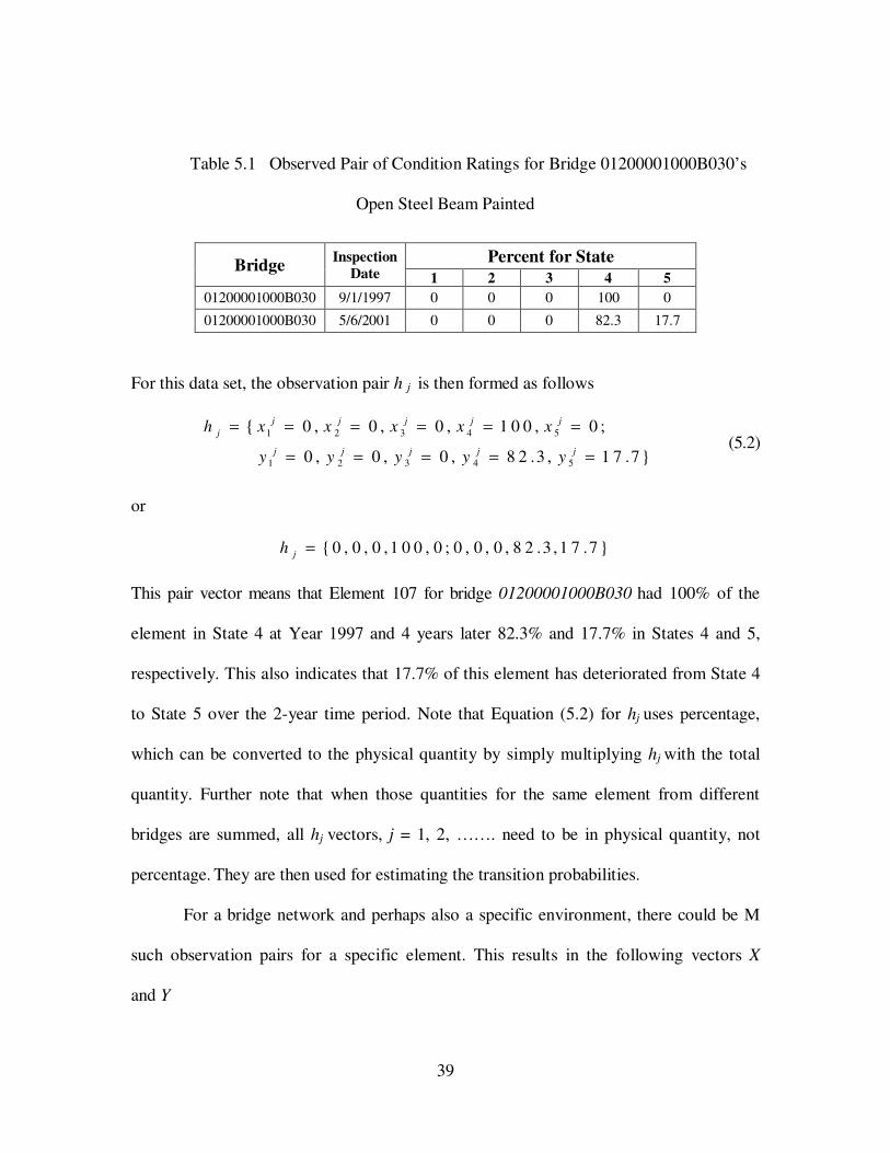
Table 5.1 Observed Pair of Condition Ratings for Bridge 01200001000B030’s
Open Steel Beam Painted
Bridge Inspection
Date Percent for State
1 2 3 4 5
01200001000B030 9/1/1997 0 0 0 100 0
01200001000B030 5/6/2001 0 0 0 82.3 17.7
For this data set, the observation pair h j is then formed as follows
1 2 3 4 5
1 2 3 4 5
{ 0 , 0 , 0 , 1 0 0 , 0 ;
0 , 0 , 0 , 8 2 .3 , 1 7 .7}
j j j j j
j
j j j j j
h x x x x x
y y y y y
= = = = = =
= = = = = (5.2)
or
{ 0 , 0 , 0 ,1 0 0 , 0 ; 0 , 0 , 0 , 8 2 .3 ,1 7 .7 }jh =
This pair vector means that Element 107 for bridge 01200001000B030 had 100% of the
element in State 4 at Year 1997 and 4 years later 82.3% and 17.7% in States 4 and 5,
respectively. This also indicates that 17.7% of this element has deteriorated from State 4
to State 5 over the 2-year time period. Note that Equation (5.2) for hj uses percentage,
which can be converted to the physical quantity by simply multiplying hj with the total
quantity. Further note that when those quantities for the same element from different
bridges are summed, all hj vectors, j = 1, 2, ……. need to be in physical quantity, not
percentage. They are then used for estimating the transition probabilities.
For a bridge network and perhaps also a specific environment, there could be M
such observation pairs for a specific element. This results in the following vectors X
and Y

40
1 , 2 , 3 , 4 , 5( )X x x x x x=
1 2 3 4 5
1 1 1 1 1
( , , , , )M M M M M
j j j j j
j j j j j
x x x x x= = = = =
= ∑ ∑ ∑ ∑ ∑ (5.3)
1 , 2 , 3 , 4 , 5( )Y y y y y y=
1 2 3 4 5
1 1 1 1 1
( , , , , )M M M M M
j j j j j
j j j j j
y y y y y= = = = =
= ∑ ∑ ∑ ∑ ∑ (5.4)
Note that after the summation these two vectors can be divided by the total quantity
1 2 3 4 5 1 2 3 4 5
1 1 1 1 1 1 1 1 1 1
M M M M M M M M M Mj j j j j j j j j j
j j j j j j j j j j
x x x x x y y y y y= = = = = = = = = =
+ + + + = + + + +∑ ∑ ∑ ∑ ∑ ∑ ∑ ∑ ∑ ∑ to express
them in percentage or probability. Pontis then uses these vectors to estimate the transition
probabilities through a regression procedure as follows.
Based on the total probability theorem, transition probabilities pki (i = 1, 2, 3, 4, 5)
need to satisfy the following equation according to the total probability theorem.
1 1 2 2 3 3 4 4 5 5 ( 1, 2, 3, 4, 5)i i i i i i iy p x p x p x p x p x == + + + + (5.5)
Note that there are five such equations in Pontis for i = 1, 2, 3, 4, 5 to include all 25
transition probabilities in the matrix defined in Equation (5.3).
Due to random behavior of deterioration and possible variation in inspection data
yi and xi (i= 1, 2, 3, 4, 5), Equation (5.5) cannot be satisfied exactly. In estimating the
transition probabilities i jp , Pontis uses the concept of regression, although there can be
other approaches to finding them. Namely, Pontis finds
such ( , 1, 2 , 3 , 4 , 5 )i jp i j = values that minimize the differences between the two
sides of Equation (5.5). This is the difference between the predicted and the observed
conditions. This difference is defined as the sum of the squared residuals as follows

41
2
i 1 1 2 2 3 3 4 4 5 5
1
2 (y -p x -p x -p x -p x -p x ) = 1, 2,3, 4, 5i
Mj j j j j j
i i i i i
j
i=
∆ = ∑ (5.6)
To minimize 2
i∆ differentiating this quantity with respect to 1 2 3 4, , , ,i i i ip p p p and
5ip , and then equating the partial derivatives to zero, we obtain the following five linear
equations as a set.
2
j 2 j j j j j j j j
1 i 1 1 2 1 2 3 1 3 4 1 4 5 1 5
1 1 1 1 1 1
j j j j 2 j j j j j j
2 i 1 2 1 2 3 2 3 4 2 4 5 2 5
1 1 1 1 1 1
j j
3 i 1 3 1 2 3
1 1
x y ( ) x x x x x x x x
x y x x (x ) x x x x x x
x y x x x
M M M M M Mj
i i i i i
j j j j j j
M M M M M M
i i i i i
j j j j j j
M M
i i
j j
p x p p p p
p p p p p
p p
= = = = = =
= = = = = =
= =
= + + + +
= + + + +
= +
∑ ∑ ∑ ∑ ∑ ∑
∑ ∑ ∑ ∑ ∑ ∑
∑ ∑3
4
j j j 2 j j j j
2 3 4 3 4 5 3 5
1 1 1 1
j j j j j j j j 2 j j
4 i 1 4 1 2 4 2 3 4 3 4 5 4 5
1 1 1 1 1 1
j j j j j j j
5 i 1 5 1 2 5 2 3 5 3 4 5
1 1 1 1
x (x ) x x x x
x y x x x x x x (x ) x x
x y x x x x x x x
M M M M
i i i
j j j j
M M M M M M
i i i i i
j j j j j j
M M M M
i i i i
j j j j
p p p
p p p p p
p p p p
= = = =
= = = = = =
= = = =
+ + +
= + + + +
= + + +
∑ ∑ ∑ ∑
∑ ∑ ∑ ∑ ∑ ∑
∑ ∑ ∑ ∑ j j 2
4 5 5
1 1
x (x )M M
i
j j
p= =
+∑ ∑ (5.7)
for 1,2,3,4,5i =
All these linear equations can be expressed in the matrix form as:
1
2
3
j 2 j j j j j j j j
1 2 1 3 1 4 1 5
1 1 1 1 1
j j 2 j j j j j j
2 1 2 3 2 4 2 5
1 1 1 1 1
j j j j 2 j j j j
3 1 3 2 3 4 3 5
1 1 1 1 1
j j j j j j
4 1 4 2 4 3
1 1
j
j
(x ) x x x x x x x x
x x (x ) x x x x x x
x x x x (x ) x x x x[ ]
x x x x x x
M M M M M
j j j j j
M M M M M
j j j j j
M M M M M
j j j j j
M M
j j j
X X
= = = = =
= = = = =
= = = = =
= = =
=
∑ ∑ ∑ ∑ ∑
∑ ∑ ∑ ∑ ∑
∑ ∑ ∑ ∑ ∑
∑ ∑ 4
5
2 j j
4 5
1 1 1
j j j j j j j j 2
5 1 5 2 5 3 5 4
1 1 1 1 1
j
j
(x ) x x
x x x x x x x x (x )
M M M
j j
M M M M M
j j j j j
= =
= = = = =
∑ ∑ ∑
∑ ∑ ∑ ∑ ∑
(5.8)
42
j j
1 i
1
j j
2 i
1
j j
3 i
1
j j
4 i
1
j j
5 i
1
x y
x y
x y[ ] 1, 2 , 3 , 4 , 5
x y
x y
M
j
M
j
M
ij
M
j
M
j
X Y i
=
=
=
=
=
= =
∑
∑
∑
∑
∑
(5.9)
1
2
3
4
5
1, 2, 3, 4, 5
i
i
i i
i
i
p
p
a p i
p
p
= =
(5.10)
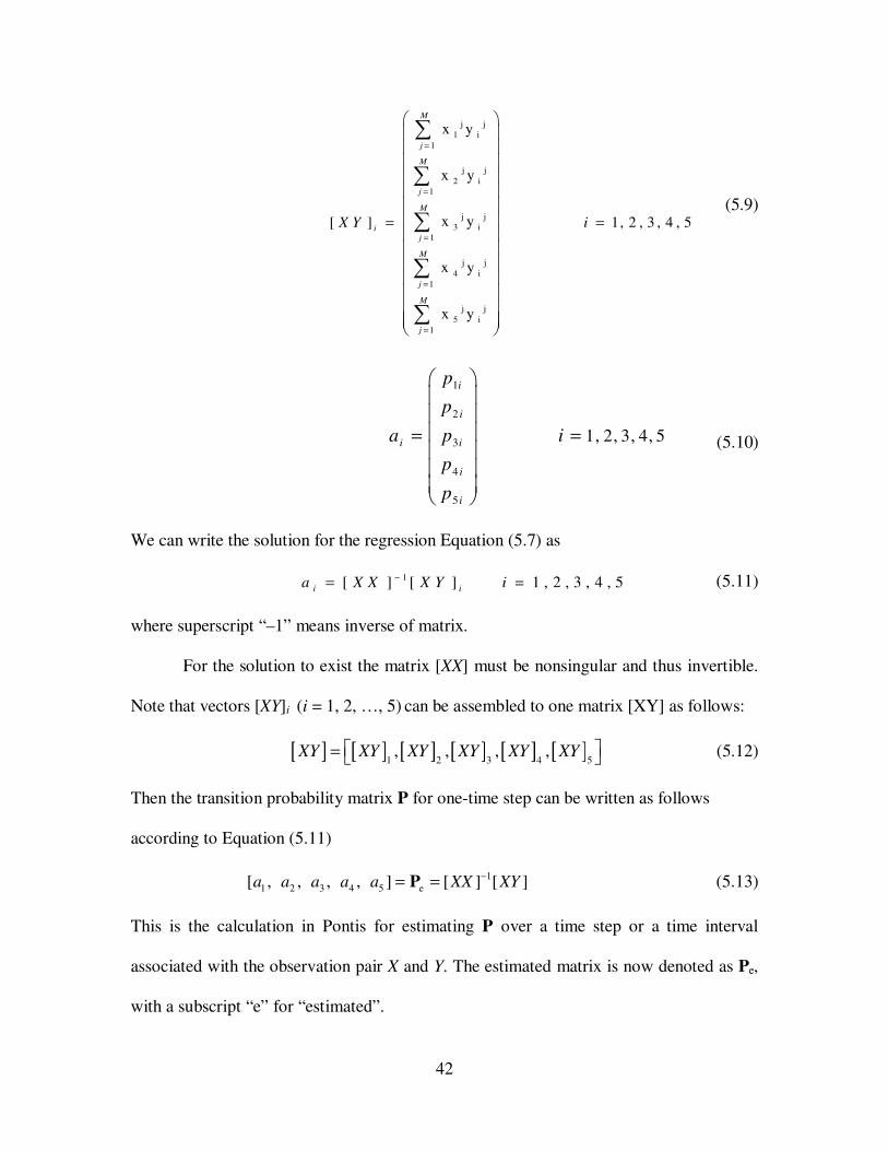
We can write the solution for the regression Equation (5.7) as
1[ ] [ ] = 1 , 2 , 3 , 4 , 5i i
a X X X Y i−= (5.11)
where superscript “–1” means inverse of matrix.
For the solution to exist the matrix [XX] must be nonsingular and thus invertible.
Note that vectors [XY]i (i = 1, 2, …, 5) can be assembled to one matrix [XY] as follows:
[ ] [ ] [ ] [ ] [ ] [ ]1 2 3 4 5, , , ,XY XY XY XY XY XY = (5.12)
Then the transition probability matrix P for one-time step can be written as follows
according to Equation (5.11)
1
1 2 3 4 5 e[ , , , , ] [ ] [ ]a a a a a XX XY−= =P (5.13)
This is the calculation in Pontis for estimating P over a time step or a time interval
associated with the observation pair X and Y. The estimated matrix is now denoted as Pe,
with a subscript “e” for “estimated”.
43
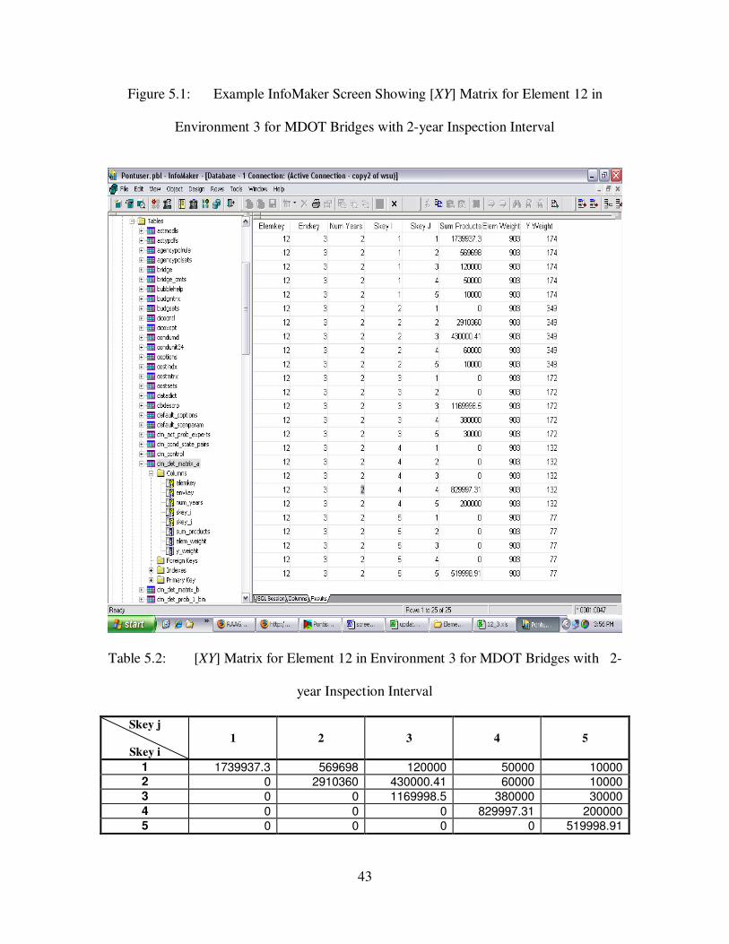
Figure 5.1: Example InfoMaker Screen Showing [XY] Matrix for Element 12 in
Environment 3 for MDOT Bridges with 2-year Inspection Interval
Table 5.2: [XY] Matrix for Element 12 in Environment 3 for MDOT Bridges with 2-
year Inspection Interval
Skey j
Skey i
1 2 3 4 5
1 1739937.3 569698 120000 50000 10000 2 0 2910360 430000.41 60000 10000 3 0 0 1169998.5 380000 30000
4 0 0 0 829997.31 200000 5 0 0 0 0 519998.91

44
As an example, Figure 5.1 shows the [XY] matrix for Element 12 in Environment
3 for MDOT bridges with an inspection interval of 2 years. The first column “Elemkey”
identifies the element number, which is 12 for this case. The second column “Envkey”
indicates the environment in which this element is in, and it is 3 for this case. The third
column “Num Years” presents the number of years between two inspections, in this case
2 years is the inspection interval selected. The fourth column “Skey I” refers to the row
for condition State i, in the [XY] matrix and the fifth column “Skey J” the column for
condition State j; these values of [XY] are assembled in Table 5.2 in matrix form for
reference. Namely in Table 5.2 and Figure 5.1, we have
;
1 2 3
1739937.3 569698 120000
0 2910360 430000.41
[ ] ; [ ] [ ] ;0 0 1169998.5
0 0 0
0 0 0
XY XY XY
= = =
4 5
50000 10000
60000 10000
[ ] ; [ ]380000 30000
829997.31 200000
0 519998.91
XY XY
= =
(5.14)
The fifth column “Sum Products” gives these components of the entire matrix [XY] in a
vector format.

45
Figure 5.2: InfoMaker Screen Showing the Values of [XX] matrix for Element 12 in
Environment 3 for MDOT Bridges with 2-Yyear Inspection Interval.
Table 5.3: [XX] Matrix for Element 12 in Environment 3 for MDOT Bridges with
2-Year Inspection Interval
Skey j
Skey i
1 2 3 4 5
1 2489282.3 354.06744 0 0 0 2 354.06744 3410010 0 0 0 3 0 0 1580000 0 0 4 0 0 0 1030000 0 5 0 0 0 0 520000

46
In Figure 5.2, the matrix [XX] defined in Equation (5.8) is shown for the same
element on Infomaker screen. The format for [XX] is the same as for [XY]. Table 5.3
shows the [XX] matrix in the matrix form for reference.
According to Equation (5.11) or (5.13), [XX] needs to be inversed to find the
estimated transition probability matrix P. This inverse is shown in Table 5.4 for the same
example of element.
Table 5.4: Inverse of [XX] Matrix for Element 12 in Environment 3 for MDOT
Bridges with 2-year Inspection Interval
([XX] matrix shown in Table 5.2)
Skey j
Skey i
1 2 3 4 5
1 0.0000004 0.0000000 0.0000000 0.0000000 0.0000000 2 0.0000000 0.0000003 0.0000000 0.0000000 0.0000000 3 0.0000000 0.0000000 0.0000006 0.0000000 0.0000000 4 0.0000000 0.0000000 0.0000000 0.0000010 0.0000000 5 0.0000000 0.0000000 0.0000000 0.0000000 0.0000019
It is seen that this [XX] matrix is inverted. However, this may not be always the
case for other possible data. For example for the same element in the same environment
for MDOT bridges but with an inspection interval 3 years, the [XX] matrix is non-
invertible. This [XX] matrix is shown in Figure 5.3 from InfoMaker and its matrix form is
shown in Table 5.5 for reference. Apparently, when inadequate data are available, the
[XX] matrix becomes not invertible. Lack of data often occurs to State 5 since usually
not many bridges or elements are kept at this worst state for a long period of time. Non-
invertible [XX] matrix may also occur when the data are not consistent, for example, for a
worst state to become better when no work was done.

47
Figure 5.3: Example InfoMaker Screen Showing [XX] Matrix for Element 12 in
Environment 3 for MDOT Bridges with 3-Year Inspection Interval
Table 5.5: [XX] Matrix for Element 12 in Environment 3 for MDOT Bridges with 3-
Year Inspection Interval
Skey j
Skey i
1 2 3 4 5
1 40000 0 0 0 0 2 0 50000 0 0 0 3 0 0 10000 0 0 4 0 0 0 10000 0 5 0 0 0 0 0

48
For the case where [XX] is invertible, i.e., Element 12 in Environment 3 for 2-year
inspection interval, Equation (5.13) gives the following result:
Pe = 1[ ] [ ]XX XY− =
2489282.3 354.06744 0.0000000 0.0000000 0.000000
354.06744 3410010 0.0000000 0.0000000 0.000000
0.0000000 0.0000000 1580000.0 0.0000000 0.000000
0.0000000 0.0000000 0.0000000 1030000.0 0.000000
0.0000000 0.0000000 0.00000
=
11739937.3 569698 120000 50000 10000
0.000000 2910360 430000.41 60000 10000
0.000000 0.000000 1169998.5 380000 30000
0.000000 0.000000 0.000000 829997.31 200000
00 0.0000000 520000.0 0.000000 0.000000 0.00000
− 0 0.000000 519998.91
0.0000004 0.0000000 0.0000000 0.0000000 0.0000000
0.0000000 0.0000003 0.0000000 0.0000000 0.0000000
0.0000000 0.0000000 0.0000006 0.0000000 0.0000000
0.0000000 0.0000000 0.0000000 0.0000010 0.0000000
0.0000000 0.0000000 0
=
1739937.3 569698 120000 50000 10000
0.000000 2910360 430000.41 60000 10000
0.000000 0.000000 1169998.5 380000 30000
0.000000 0.000000 0.000000 829997.31 200000
.0000000 0.0000000 0.0000019 0.000000 0.000000 0.
000000 0.000000 519998.91
0.70 0.23 0.05 0.02 0.0
0.00 0.85 0.13 0.02 0.00
0.00 0.00 0.74 0.24 0.02
0.00 0.00 0.00 0.81 0.19
0.00 0.00 0.00 0.00 1.00
=
(5.15)
This estimated transition probability matrix is for time steps with a length of 2 years.
It is seen in Equation (5.15) that p13, p14, p15, p24, p25, p35, p21, p31, p32, p41, p42, p43,
p51, p52, p53, and p54, are not necessarily zero. For example p13 = 0.05, p14 = 0.02, p24 = 0.02,
p35 = 0.02. This is because the regression process does not require all these terms to be
zero. In addition each row also may not add to 1, again because it is not required in the
regression approach used in Pontis.
Nevertheless, after the calculation shown in Equation (5.15), Pontis takes only the
diagonal terms for the transition probability matrix, sets a zero to p13, p14, p15, p24, p25, p35,

49
p21, p31, p32, p41, p42, p43, p51, p52, p53, p54, compute1- p11 as p12, 1- p22 as p23, 1- p33 as p34,
1- p44 as p45, and sets 1 to p55. Now the rows are forced to add to 1.0.
5.2 Combination of Estimated Transition Probability Matrices for Different
Time-Steps
In reality, not all “before” and “after” inspections are done with an exactly same
constant time difference or interval. For example, bridge inspections may be performed
with several months apart to several years apart, although 2 years apart is the norm in the
US. Inspection data obtained with different time intervals should not be mixed in one
estimation calculation as formulated in Equation (5.13). For example, three one-year
transition probability matrices multiplied with each other gives a three-year matrix, which
should not be mixed with one-year matrices.
Instead, the data need to be grouped according to the length of inspection interval.
For each group with the same inspection interval, Equation (5.13) can be computed,
which will result in P for that particular inspection interval or time step. In order to
combine these transition probability matrices estimated using data with different time
intervals, Pontis does offer a function to do just that, which is presented below.
Based on the homogeneous Markov Chain concept, the transition probability
matrix for n-step (over n time intervals) is defined as the product of n one-step (one-time
interval) transition probability matrices:
T T T
n m a tr ic e s m u lt ip lie d
.. .... . T
n =P P P P14424 43 (5.16)
According to this concept, Pontis determines a transition probability matrix P for one
year as one-step by combining equivalent one-step (one-year) transition matrices. Each of
50
the equivalent one-step matrices is obtained from an n-step (n-year) matrix. This
weighted combination is done one row at a time because the weight for each row of each
matrix can be different.
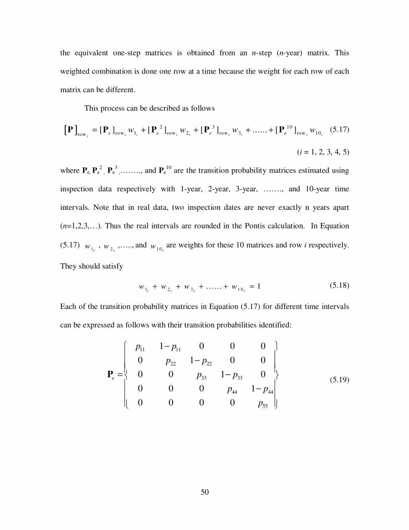
This process can be described as follows
[ ]i i i ii
2 3 10
row 1 row 2 row 3 row 10row[ ] [ ] [ ] ...... [ ]
i i i ie e e ew w w w= + + + +P P P P P (5.17)
(i = 1, 2, 3, 4, 5)
where Pe, Pe2
, Pe3
,…….., and Pe10
are the transition probability matrices estimated using
inspection data respectively with 1-year, 2-year, 3-year, ……., and 10-year time
intervals. Note that in real data, two inspection dates are never exactly n years apart
(n=1,2,3,…). Thus the real intervals are rounded in the Pontis calculation. In Equation
(5.17) 1
wi
, 2
wi
,….., and 1 0
wi
are weights for these 10 matrices and row i respectively.
They should satisfy
1 2 3 1 0... .. . 1w w w w+ + + + =
i i i i (5.18)
Each of the transition probability matrices in Equation (5.17) for different time intervals
can be expressed as follows with their transition probabilities identified:
11 11
22 22
33 33
44 44
55
1 0 0 0
0 1 0 0
0 0 1 0
0 0 0 1
0 0 0 0
e
p p
p p
p p
p p
p
− −
= − −
P (5.19)
51
Pe 2
2 2
11 11
2 2
22 22
2 2
33 33
2 2
44 44
2
55
1 0 0 0
0 1 0 0
0 0 1 0
0 0 0 1
0 0 0 0
p p
p p
p p
p p
p
− −
= −
−
(5.20)
Pe 3
3 33 311 11
3 33 322 22
3 33 333 33
3 33 344 44
3355
1 0 0 0
0 1 0 0
0 0 1 0
0 0 0 1
0 0 0 0
p p
p p
p p
p p
p
− −
= −
−
(5.21)
M
M
Pe n
11 11
22 22
33 33
44 44
55
1 0 0 0
0 1 0 0
0 0 1 0
0 0 0 1
0 0 0 0
n nn n
n nn n
n nn n
n nn n
nn
p p
p p
p p
p p
p
− −
= −
−
(5.22)
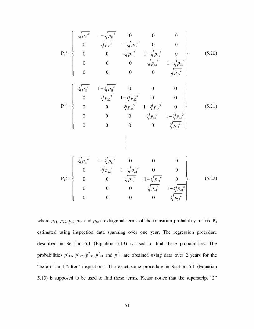
where p11, p22, p33, p44 and p55 are diagonal terms of the transition probability matrix Pe
estimated using inspection data spanning over one year. The regression procedure
described in Section 5.1 (Equation 5.13) is used to find these probabilities. The
probabilities p2
11, p2
22, p2
33, p2
44 and p2
55 are obtained using data over 2 years for the
“before” and “after” inspections. The exact same procedure in Section 5.1 (Equation
5.13) is supposed to be used to find these terms. Please notice that the superscript “2”

52
here indicates the time interval of 2 years, and it is not an exponent. Similarly pn
11, pn
22,
pn
33, pn
44, and pn
55 are the same except using data over n years.
It is seen in Equations (5.19) to (5.22) that the diagonal terms of the transition
probability matrix for n years are taken nth
root for n = 2, 3, …….,10 to be combined with
the one-year matrix as defined in Equation (5.17). Further, all other probabilities in the
matrices are set to zero except the ones next to the diagonal terms to the immediate right,
as discussed earlier. This is done based on two assumptions: 1) the condition will not
improve without repair or rehabilitation; 2) deterioration will not take place in the form of
skipping a condition state (i.e., from State 1 to 3, from State 2 to 4, or from State 3 to 5).
The second assumption may be true for short time periods such as one or two years, but
questionable for longer periods such as 8, 9, and 10 years. Practically, however, this is
not a serious concern at this point, because perhaps no bridge was inspected that many
years apart. Nevertheless, transition probabilities over 3 or 4 years may very well be non-
zero skipping a state. Equation (5.24) shows an example of a 6.0% transition probability
for States 1 to 3, 6.8% from State 2 to 4, and 8.3% from States 3 to 5, for Element 12 in
Environment 3 of Michigan. Ignoring these (i.e., setting them to zero) apparently will
result in a lower deterioration rate.
The weights in Equation (5.17) are set in Pontis as follows, depending on the
number of data pairs used to estimate Pe, Pe2
, Pe3
,…….., Pe10
for each row , respectively
j i
j i
k i
k
Nw
N=∑
i= 1, 2, 3,…,5; j= 1, 2, 3,…,10 (5.23)
where Nji is the number of data pairs with j-years apart and transition (deterioration)
starting from State i, used to estimate probability matrix Pei. For example, Figure 5.4

53
shows an example of 6iN for Pe6 and i = 1, 2, 3, 4, 5. The first column “Elemkey”
indicates Element 12, “Envkey” for Environment 3, “Num Years” for inspection interval
6 years, “Skey” for row i = 1, 2, 3, 4, 5, and “Weight” for 6iN in Equation (5.23). In
other words, the more data pairs are used for a transition probability matrix, the heavier
the resulting matrix will be weighted when combined with other matrices for different
years. Also the more data pairs there are for a row in a matrix, that row will be weighted
more when combined with the same row in other matrices.
Figure 5.4: Example Infomaker Screen for Combination Weights

54
Note that the combined resulting transition matrix is to be applied to the same
element from all the bridges in the same environment and for all the future years, based
on the homogenous Markov Chain assumption discussed in Chapter 3. Since that matrix
is for one-step equal to one year, for n-step (n-year) transition, n one-year matrices will
be multiplied to obtain the n-year transition probability matrix, according to Equation
(5.16). Then it is multiplied by the corresponding initial distribution to find the predicted
condition distributions in the future.

55
CHAPTER 6 LIMITATIONS IN THE PONTIS APPROACH
This chapter discusses several issues related to Pontis in estimating the transition
probability matrix for “do-nothing” action to be used in bridge element condition
prediction. As discussed earlier this transition probability matrix is critical because the
predicted long-term deterioration can be significantly affected.
6.1 Non-invertible [XX] Matrix:
Equation (5.13) shows that the [XX] matrix needs to be inverted to obtain the
estimated transition probability matrix Pe. In other words, if [XX] is not invertible, Pe
cannot be found. When this occurs it appears that Pontis sets certain values in the [XX]
matrix to make it invertible so that the calculation can proceed. For the example of
Element 12 in Environment 3 discussed in Chapter 5 for 3-year inspection interval the
[XX] matrix is not invertible. This [XX] matrix was shown in Table 5.5.
Though the [XX] matrix is not invertible Pontis still outputs transition
probabilities. Figure 6.1 shows these transition probability values from InfoMaker. The
first column “Elemkey” identifies the element number, which is 12 for this case. The
second column “Envkey” indicates the environment in which this element is in, and it is
3. The third column “Num Years” presents the number of years between two inspections,
in this case 3 years is the inspection interval selected. The fourth column “Skey” refers to
the row of condition States (i.e., first row for State 1, second for State 2, ….., fifth for
State 5). The fifth column “Prob Value” gives the transition probability corresponding to
the respective “Skey”. The last column “Weight” is respective 3iN i =1, 2, 3, 4, 5.

56
Figure 6.1: InfoMaker Screen Showing Transition Probabilities for Element 12 in
Environment 3 for MDOT Bridges with 3-Year Inspection Interval
([XX] Matrix Non-invertible but Transition Probabilities Obtained)
It appears that a 1 is added to p55 to obtain the inverse of the [XX] matrix and then
the calculation proceeds. This needs to be further investigated to fully understand the
procedure used for making the matrix invertible. Further the implications of this
procedure to the future distribution prediction also need to be fully understood.
6.2 Negative Transition Probabilities
Another issue with the Pontis approach is that negative transition probabilities
may be found in the regression procedure formulated in Equation (5.13). According to

57
the theory of probability, no probability should be smaller than 0 or negative. However
negative transition probabilities may result from Equation (5.13) as shown in the
following example.
Consider Element 107 in Environment 1 for MDOT bridges with an inspection
interval of 2 years. The InfoMaker screen showing the [XY] matrix for this case is given
in Figure 6.2 and the same assembled in the matrix form is shown in Table 6.2.
Figure 6.2: InfoMaker Screen of [XY] Matrix for Element 107 in Environment 1 for
MDOT Bridges with 2-Year Inspection Interval
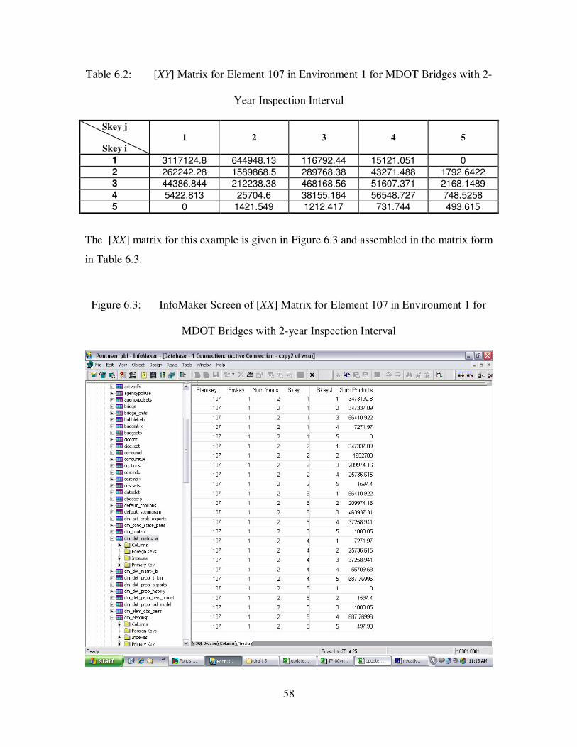
58
Table 6.2: [XY] Matrix for Element 107 in Environment 1 for MDOT Bridges with 2-
Year Inspection Interval
Skey j
Skey i
1 2 3 4 5
1 3117124.8 644948.13 116792.44 15121.051 0 2 262242.28 1589868.5 289768.38 43271.488 1792.6422 3 44386.844 212238.38 468168.56 51607.371 2168.1489 4 5422.813 25704.6 38155.164 56548.727 748.5258 5 0 1421.549 1212.417 731.744 493.615
The [XX] matrix for this example is given in Figure 6.3 and assembled in the matrix form
in Table 6.3.
Figure 6.3: InfoMaker Screen of [XX] Matrix for Element 107 in Environment 1 for
MDOT Bridges with 2-year Inspection Interval

59
Table 6.3: [XX] Matrix for Element 107 in Environment 1 for MDOT Bridges with
2-Year Inspection Interval
Skey j
Skey i
1 2 3 4 5
1 3473192.8 347337.09 66410.922 7271.97 0 2 347337.09 1602700 209974.16 25736.615 1597.4 3 66410.922 209974.16 463937.31 37258.941 1088.85 4 7271.97 25736.615 37258.941 55709.68 687.76996 5 0 1597.400 1088.85 687.76996 497.98
For this case the [XX] matrix is invertible and the inverse result is given in Table
6.4 computed using Excel. Transition probabilities for this case is calculated using
Equation (5.13) and the results are presented in Table 6.5.
Table 6.4: Inverse Matrix for [XX] Matrix for Element 107 in Environment 1 for
MDOT Bridges with 2-Year Inspection Interval
Skey j
Skey i
1 2 3 4 5
1 0.0000003 -0.0000001 0.0000000 0.0000000 0.0000002 2 -0.0000001 0.0000007 -0.0000003 -0.0000001 -0.0000014 3 0.0000000 -0.0000003 0.0000024 -0.0000014 -0.0000023 4 0.0000000 -0.0000001 -0.0000014 0.0000192 -0.0000231 5 0.0000002 -0.0000014 -0.0000023 -0.0000231 0.0020497
Table 6.5: Transition Probability Matrix for Element 107 in Environment 1 for
MDOT Bridges with 2-year Inspection Interval
Skey j
Skey i
1 2 3 4 5
1 0.90 0.09 0.01 0.00 0.00 2 -0.03 0.97 0.05 0.01 0.00 3 -0.02 0.01 0.98 0.03 0.00 4 0.01 0.00 0.00 0.99 0.00 5 0.13 -0.28 0.12 0.01 0.99

60
Pontis then takes the diagonal terms 0.90, 0.97, 0.98, 0.99, and 0.99 as p11, p22,
p33, p44 and p55. Further it calculates P12 = 1 – p11, p23 = 1 - p22, p34 = 1 – p33, p45 = 1 –
p44 and ignores the negative probabilities.
Although it appears that the transition probabilities shown in Pontis are not
negative, the negative probabilities shown in Table 6.5 actually have affected the
probabilities on the diagonal, because they were obtained from the same process defined
in Equation (5.13).
6.3 Possible Non-zero p13, p14, p15, p24, p25, p35, p21, p31, p32, p41, p42, p43, p51, p52, p53,
and/or p54 values
In Table 6.5, p13 = 0.01 and p24 = 0.01. They show an example of non-zero
probabilities for transitions skipping a state level, namely from State 1 to State 3 and
State 2 to State 4. Recall that we have seen another such case earlier. Apparently, this
situation violates one of the assumptions used in Pontis that such skipping transition is
impossible. As a matter of fact, data showing such skipping are excluded in Pontis in the
stage of valid pair identification i.e., when X and Y are identified in Equation (5.3) and
(5.4). However, the regression procedure defined in Equation (5.13) does not eliminate
such possibility of having transition probabilities become non-zero.
Furthermore, Table 6.5 shows p32 = 0.01, p51 = 0.13, p53 = 0.12, p54 = 0.01, which
also violates another assumption in Pontis that the probabilities of transition from a worse
state to a better states are zero indicating no MR&R action is taken. Again these non-zero
values affect the probabilities on the diagonal.

61
Note also that theoretically the diagonal terms in the estimated transition
probability matrix Pe can become negative, and other off diagonal terms can become non-
zero or even negative. It is because the regression process defined in Equation (5.13) does
not prevent these possibilities. This, situation may also cause the diagonal terms (p11, p22,
p33, p44, p55) taken in Pontis for future prediction to become unreliable. Thus, this is a
significant issue related to using the Pontis approach for future condition prediction and
the related optimization for MR&R action.

62
CHAPTER 7 PROPOSED METHOD OF TRANSITION
PROBABILITY ESTIMATION
7.1 Optimization Formulation for Estimating Transition Probabilities
The Pontis approach to estimating the homogenous transition probability matrix
focuses on the error or difference between the predicted probabilistic conditions and the
inspection based conditions (or measured conditions). After formulating this sum of
errors for all the inspection data used for estimation, a formal minimization procedure is
applied to find the appropriate transition probabilities such that the error sum is reduced
to the minimum. This process produces the minimizing transition probability matrix.
Again this matrix is constant for all ages of the element.
A similar approach is adopted here for estimating the non-homogeneous transition
probability matrices. Namely the error or the difference between the predicted and
measured bridge element conditions is minimized. Since the element conditions are
associated with a probability distribution, the mean of the distribution is used for this
optimization. Namely, estimating the transition probability matrices is accomplished
here by minimizing the sum of the differences between the inspection based conditions
and the predicted conditions. The prediction process no longer assumes a constant
transition probability matrix as for the homogeneous Markov Chain. Instead, the
following formulation is developed in this project for estimating or identifying the age
dependent (i.e., non-homogeneous) transition probability matrices for each bridge
element:

63
Minimize Σi=1,…,N | Yi – Predicted [Yi, P(Ai)]|2
(7.1)
Subject to Σk=1,2,...,5 pjk(Ai) = 1 for all j
pjk(Ai) > 0 for all k and j
where N = total number of condition transitions used (i.e., the number of data pairs used);
Yi = condition state vector right after the ith transition (for ith pair of transition data);
Predicted [Yi, P(Ai)] = Predicted condition state vector for the same element involved in
the ith transition, using the transition probability matrix P(Ai) depending on the element’s
age Ai. The symbol |x| means the magnitude or modulus of vector x. The transition
probabilities p are the elements of the matrix P. The conditions for them to meet in
Equation (7.1) are there to satisfy Equation (3.8) for consistency. These conditions are
met in Pontis, rather, after the transition probability matrix is found, by simply setting p
values equal to 0 if obtained negative, or the diagonal terms 1.0 if obtained to be larger
than 1.0.
Note also that the Markov Chain model used here is more general than the Pontis’
homogeneous model, for its non-homogeneity. Therefore, the transition probability
matrices P(A) are shown as functions of age A. It means that P(Ai) can be different
according to age Ai of the element involved in transition i. For application to bridge
management focused herein, we consider only the effect of age, not the absolute time.
This can be seen more easily in a simple application example in the next section.

64
7.2 A Simple Illustrative Example
Consider Element 215 (reinforced concrete abutment) in Environment 1 for the
MDOT bridges with an inspection interval of 2 years. So tn – tn-1 is 2 years for this
example. A sample set of 3 pairs of condition transition data for this element is used in
this example for illustration, as displayed in Table 7.1. For this element, the total number
of condition states is 4 (i.e., S=4).
Table 7.1 Sample Data for Element 215 in Environment 1 for MDOT
Bridge Key age-x X1 X2 X3 X4 age-y Y1 Y2 Y3 Y4
16116021000B010 3 1.00 0.00 0.00 0.00 5 0.93 0.07 0.00 0.00
15115051000B010 36 0.94 0.06 0.00 0.00 38 0.89 0.11 0.00 0.00
05105011000B010 42 0.95 0.05 0.00 0.00 44 0.84 0.16 0.00 0.00
In this table, column “Bridge Key” is the identification for each bridge. Column “age-x”
records the age of the element at time tn-1 for this case (Year 1995), and similarly “age-y”
the age at time tn (Year 1997). Column X1 shows the percentage of element 215 in
Condition State 1 in the bridge at time tn-1 (Year 1995). Similarly, X2, X3, and X4 are the
percentages of the element in Condition States 2, 3, and 4 respectively at time tn-1, and Y1,
Y2, Y3, and Y4 at time tn (Year 1997).
For easy illustration without loss of generality, it is assumed that for the age
range of 0 to 20 years, the transition probability matrices for every two years are constant
and designated as U0-20. The subscript 0-20 indicates the applicable age range. For the
age range of 21 to 40 years, another constant transition probability matrix V21-40 is used to

65
model the transition (deterioration) for every 2 years in the same format. For the age
range of 41 and older, a third transition probability matrix W41- is used to model transition
(deterioration) for every two years also in the same format but without specifying the
ending age. Since the sample data set includes bridges only up to 42 years of age, no
further transition probability matrices could be used. Otherwise more matrices would be
considered and used for modeling. The indefinite upper age limit for W41- means that for
ages older than 41 years, this transition probability matrix is to be used for prediction.
Accordingly, Equation (7.1) is specifically formulated as follows for N=3:
Minimize | {0.93, 0.07, 0.00, 0.00} – {1.00, 0.00, 0.00, 0.00} U0-20|2
+ | {0.89, 0.11, 0.00, 0.00} – {0.94, 0.06, 0.00, 0.00} V21-40 |2
+ | {0.84, 0.16, 0.00, 0.00} – {0.95, 0.05, 0.00, 0.00} W41- |2
(7.2)
Subject to Σk=1,2,...,4 ujk,0-20 = 1 for all j, and ujk,0-20 > 0 for all k and j
Σk=1,2,...,4 vjk,21-40 = 1 for all j, and vjk,21-40 > 0 for all k and j
Σk=1,2,...,4 wjk,41- = 1 for all j, and wjk,41- > 0 for all k and j
The lower case non-bolded letters u, v, and w are the transition probabilities in the
matrices U0-20, V21-40, and W41-, with the age applicability ranges also indicated. The first
term in the magnitude signs |.| is associated with the first bridge “16116021000B010”,
where the first vector {0.93, 0.07, 0.00, 0.00} is the probability distribution of the

66
element condition for this bridge after the transition at time tn (Year 1997). The second
half in the magnitude signs (i.e., the terms after the minus sign) is a product of a vector
and the transition probability matrix. The vector in the big brackets is the probability
distribution of the element condition of that bridge at time tn-1 (Year 1995). This vector
multiplied with the transition probability matrix U0-20 gives the predicted probability
distribution of the element condition state at time tn (Year 1997). The following two
magnitudes squared have the same physical meaning and structure as the first one but for
the other two bridges. Then the transition probability matrices U0-20, V21-40, and W41- are
to be found to have the sum of the differences or errors minimized. In this example, the
following probabilities are pre-set for impossible transitions and consistency,
respectively.
ujk,0-20 =0 if j > k; ujk,0-20 =1 – ujj,0-20 if k-j=1; 0 otherwise
vjk,21-40 =0 if j > k; vjk,21-40 =1 – vjj,21-40 if k-j=1; 0 otherwise
wjk,41- =0 if j > k; wjk,41- =1 – wjj,41- if k-j=1; 0 otherwise
u44,0-20 = v44,21-40 = w44,41- = 1 (7.3)
This makes only the first three diagonal terms in each of the three transition probability
matrices unknown to be found in the minimization process: u11,0-20; u22,0-20; u33,0-20 ;
v11,21-40 ; v22,21-40; v33,21-40 ; w11,41- ; w22,41- ; w33,41- .
As noted earlier, Equation (7.2) is a simple example of Equation (7.1) in that the
transition probability matrices U0-20, V21-40, and W41- are constants respectively for age
ranges 0 to 20 years, 21 to 40 years, and 41 years and older. In other words, the
transition rates or deterioration rates are assumed constant within each of the specified

67
age ranges, but variable for the entire service life of the element. In general, the
transition probabilities over each of the 20-year or longer periods may not be very
constant. The model in Equation (7.1), nevertheless, allows more general cases of one
transition probability matrix for each time unit of interest. On the other hand, the number
of unknown transition probabilities to be found will accordingly increase and the required
computation effort. However, for certain bridge elements with low deterioration rates
(i.e., those with long service lives), assuming a constant transition probability matrix for a
number of years is not unreasonable. It is because the rate (or probability) of transition
from a better state to a worse state (or the rate of deterioration) for this situation is
relatively low, and thus variation of this rate from year to year is not significant.
Therefore a constant transition probability matrix for an age range may be realistic and
practical.
It may be also interesting to point out that the Pontis approach based on
homogeneous Markov Chain actually can be viewed as a special case of non-
homogeneous Markov Chain, with only one constant transition probability matrix for all
time periods over the entire life span of the element.
7.3 An Application Example
In this application example, the same Element 215 is used. The inspection data of
the element are taken from the MDOT Pontis database. It is well known that high quality
of input data can never been over-emphasized. We thus have examined the data cleaning
procedure used in Pontis and found that the process is not consistent enough because it
misses invalid pairs. We have thus developed a more rigorous data cleaning procedure,

68
which has been used here to screen out invalid data pairs that were not identified by the
Pontis screening process. A typical example is presented below for illustration:
Table 7.2: Condition State Distribution for Element 215 in MDOT Bridge
27127022000B030 in Environment 1
(0)X
(0)
1x (0)
2x (0)
3x (0)
4x
In % 77.778 14.815 7.407 0 (1)
Y (1)
1y (1)
2y (1)
3y (1)
4y
In % 0 96.296 3.704 0
In this table, as indicated earlier in this report, vectors (0)X and
(1)Y are the
condition state distribution in the previous year and the current years respectively. Note
that the sum of (0)
1x and (0)
2x for condition states 1 and 2 should be greater than or equal to
the sum of (1)
1y and (1)
2y , because the latter two quantities can only come from the former
two for the do-nothing situation. However, it is not true as seen in Table 7.2, as the sum
of (0)
1x and (0)
2x is 92.593, which is less than the sum of (1)
1y and (1)
2y , 96.296, in Table 7.2.
There is a number of possible causes for the sum of (1)
1y and (1)
2y to be larger than that of
(0)
1x and (0)
2x . 1) Simple error of input such as typo. 2) Some quantity from (0)
3x has
moved to (1)
2y for improvement in condition, which violates the “Do-Nothing”
assumption. Our screening algorithm targets at such observed inconsistencies.
In this first step of development work, to avoid the issue of collectively using data
with different inspection intervals and weighting them differently, only the pairs with 2-
year inspection interval for Element 215 are used here in this example. So tn – tn-1 = 2
years is used with approximation of rounding. Equation (7.1), as specified in Equation

69
(7.3), is applied, except that more data pairs are included, using all available MDOT data
up to Year 2000.
It should be noted that Equation (7.1) for estimating non-homogeneous transition
probability matrices can easily accommodate data obtained with different inspection
intervals, such as 2, 3, or any other number of years. In Pontis, in contrast, data from
unevenly intervaled inspections are grouped according to the inspection interval, because
mixing them would cause unacceptable approximation. Namely, data with 1-year
intervals (with rounding) are put in one group, 2-year intervals (also with rounding) in
another group, and so on. Each group is used separately for estimating the transition
probability matrix for that group. Then the resulting matrices for different groups are
averaged with weights proportional to the number of data pairs used in each group. This
approach also requires critical examination, because longer intervaled inspection data
usually are more reliable than those shorter intervaled. For example, a data pair
intervaled by one year is usually not as good in quality as another pair separated for
longer time. It is because for shorter intervals, the condition change is very little and the
inspection results may not reflect such fine changes. In the Pontis approach, however,
this higher quality data pair intervaled longer is treated the same way as another pair
intervaled more closely.
In applying Equation (7.1) to this data set, three transition probability matrices are
used to model the element’s deterioration: U0-20, V21-40, and W41- , as done in the small
problem shown previously. They respectively cover age ranges of 0 to 20 years, 21 to 40
years, and 41 years and beyond.

70
Using inspection data up to Year 2000, Table 7.3 shows the resulting transition
matrices U0-20, V21-40, and W41- for Environment 1 in Michigan, compared with the
constant transition probability matrix obtained using the Pontis approach. According to
Equation (7.3) only the 9 probabilities on the diagonal are the unknowns. Table 7.3
displays these 9 terms, along with the last terms in the probability matrices (u44=
v44=w44=1). Since this last term is not treated as an unknown for the non-homogeneous
Markov Chain approach, it is shown lightened.
It is seen in Table 7.3 that the Pontis transition probabilities are mostly between
the maximum and minimum values of those in the matrices U0-20, V21-40, and W41-. This
actually shows the essence of the homogeneous Markov Chain application here:
modeling a non-homogeneous Markov Chain with compromise. Nevertheless,
constrained by the homogeneity assumption, it would not be able to realistically model
the non-homogeneous stochastic process. For projecting to a far future, the difference
between the two approaches can be significant.
For other three environments, similar comparisons are observed, showing the
Pontis obtained transition matrices to be a compromise to fit the data. This is seen more
clear in Table 7.4 when the non-homogeneous Markov Chain approach used 6 transition
probability matrices U, V, W, X, Y, and Z (instead of three tried first) to respectively
cover age ranges of 0-10, 11-20, 21-30, 31-40, 41-50, and 51 years and older.

71
Table 7.3 Comparison of Transition Probability Matrices between the Proposed
Method Using 3 Matrices, Pontis Approach, and Arithmetic Method for Element 215 in
Environment 1
p11 p22 p33 p44
U0-20 0.977 0.986 1.000 1.000
V21-40 0.968 0.986 0.941 1.000
W41- 0.960 0.982 1.000 1.000
Pontis 0.963 0.985 0.990 1.000
Arithmetic 0.962 0.963 1.000 1.000
Table 7.4 Comparison of Transition Probability Matrices between the Proposed
Method Using 6 Matrices, Pontis Approach, and Arithmetic Method for Element 215 in
Environment 1
p11 p22 p33 p44
U0-10 0.972 0.989 0.995 1.000
V11-20 0.989 0.980 0.990 1.000
W21-30 0.973 0.959 0.990 1.000
X31-40 0.966 0.992 0.978 1.000
Y41-50 0.949 1.000 0.990 1.000
Z51- 0.967 0.976 0.999 1.000
Pontis 0.963 0.985 0.990 1.000
Arithmetic 0.962 0.963 1.000 1.000
To evaluate the proposed non-homogeneous Markov Chain approach, the
resulting transition probabilities are used to predict the element’s immediate future
72
distribution vector at the network level. Then this predicted distribution is compared with
the measured distribution vector using the inspection data. A relative error is then
calculated to quantitatively evaluate the effectiveness of the prediction. It is important to
note that this future distribution vector based on inspection results was not used in the
process of estimation for the transition probabilities. Essentially, this evaluation
simulates a practical application of using the latest inspection data to predict the future
bridge condition at the network level. Tables 7.5 and 7.6 display the results for this
evaluation between the proposed approach and the Pontis approach, using the Element
215 data of MDOT. Largely as expected, the proposed approach has produced smaller
errors, mainly due to the higher modeling resolution using several transition probability
matrices for the entire life span of the element. This is also seen more clearly when
comparing the results of Table 7.5 to those in Table 7.6. It is seen that using 6 transition
probability matrices (each covering about 10 years except the last matrix) has performed
generally better than using 3 matrices (each covering about 20 years except the last
matrix).
Note also that when Year 2002 data are used for evaluation, inspection data up to
Year 2000 are used for estimating the transition probability matrices. When Year 2004
data are used for evaluation, inspection data up to Year 2002 are used for the estimation.
Again this is to simulate a case of realistic practice of bridge management. These cases
are indicated in Tables 7.5 and 7.6.
For comparison, the arithmetic method presented earlier is also applied to this
example, and the results are included in both Tables 7.5 and 7.6. It is seen that that
method did not perform as well as the Pontis and the proposed approaches. It is

73
understood that the main reason for this performance is its lack of statistical foundation of
the arithmetic method. That method simply “fits” the data into the assumed structure of
the transition probability matrix. Therefore, it cannot be expected to predict the future
behavior of the element’s deterioration.
Table 7.5 Comparison of Errors (in %) for Proposed Method Using 3 Matrices, Pontis
Approach, and Arithmetic Method – Element 215
Using 2002
data for
evaluation
Using 2004
data for
evaluation
Using 2002
data for
evaluation
Using 2004
data for
evaluation
Env1
Proposed
Approach 2.11 3.05
Env3
Proposed
Approach 5.67 1.01
Pontis
Approach 2.89 3.88
Pontis
Approach 7.11 2.03
Arithmetic
Method 2.72 4.07
Arithmetic
Method 7.54 2.19
Env2
Proposed
Approach 3.12 3.95
Env4
Proposed
Approach 1.95 6.10
Pontis
Approach 3.83 4.48
Pontis
Approach 2.82 6.97
Arithmetic
Method 3.80 4.27
Arithmetic
Method 3.7 7.44
Table 7.6 Comparison of Errors (in %) for Proposed Method Using 6 Matrices, Pontis
Approach, and Arithmetic Method – Element 215
Using 2002
data for
evaluation
Using 2004
data for
evaluation
Using 2002
data for
evaluation
Using 2004
data for
evaluation
Env1
Proposed
Approach 2.04 3.00
Env3
Proposed
Approach 6.81 0.94
Pontis
Approach 2.89 3.88
Pontis
Approach 7.11 2.03
Arithmetic
Method 2.72 4.07
Arithmetic
Method 7.54 2.19
Env2
Proposed
Approach 2.89 2.99
Env4
Proposed
Approach 1.50 5.81
Pontis
Approach 3.83 4.48
Pontis
Approach 2.82 6.97
Arithmetic
Method 3.80 4.27
Arithmetic
Method 3.7 7.44

74
It is worth mentioning that, again, more transition probability matrices can be
used in the proposed non-homogeneous Markov Chain model to improve modeling when
warranted. Of course, this will increase the requirement for computation effort.
It is also important to note that the Pontis approach for estimating the transition
probability matrix may cause a probability value to become negative and the sum of a
row not to add to 1, especially when the number of valid data pairs is small. This
problem is completely avoided or resolved in formulating the optimization problem of
Equation (7.1), shown in Equation (7.3) for this example as the constraints for
minimization. The condition of Equation (3.8) (i.e., non negative probabilities summed
to 1.0 for each row) can be enforced as in Equation (7.3). The optimization process as
formulated in Equation (7.1) then will not produce those violating values as solutions.
Note that the Pontis approach, though, is different for enforcing these constraints. It
rather solves a least square fitting problem by minimizing the squared error sum without
avoiding these violating values. When such values do result, they are simply deleted and
then replaced by artificially determined values. Therefore, the Pontis approach is not
expected to produce reliable results every time when applied. This is seen in the results in
Tables 7.5 and 7.6. It is also seen in the results for more elements presented next.
7.4 More Application Examples and Discussions
More elements are used in this section for application of the proposed non-
homogeneous Markov Chain modeling and prediction. They include Elements 104, 106,
and 210. The results will have both the three and six matrix cases as done above.
Tables 7.7 and 7.8 show the results for Element 104 - Precast Prestressed Box Beams.

75
Table 7.7 Comparison of Errors (in %) for Proposed Method Using 3 Matrices,
Pontis Approach, and Arithmetic Method – Element 104
Using
2002 data for
evaluation
Using 2004
data for
evaluation
Using
2002 data for
evaluation
Using
2004 data for
evaluation
Env1
Proposed
Approach 0.06 0.01
Env3
Proposed
Approach 0.69 0.35
Pontis
Approach 0.06 0.35
Pontis
Approach 1.85 1.04
Arithmetic
Method 0.06 0.35
Arithmetic
Method 1.88 1.04
Env2
Proposed
Approach 0.26 0.07
Env4
Proposed
Approach 0.48 0.34
Pontis
Approach 0.78 0.03
Pontis
Approach 0.44 0.36
Arithmetic
Method 1.08 0.04
Arithmetic
Method 0.44 0.44
It is shown in Table 7.7 that the first set of results for Environment 1 using year
2002 data for evaluation involves the same error for all three approaches used. The
reason for this is that there is no deterioration for all the data points (data pairs) used for
estimating the transition probabilities. To be exact, there are 38 data points for this
environment, and all of them have 100% of the element in State 1 before and after
inspection. Thus the estimations of the transition probabilities or their interpretations
using these different methods actually lead to the same result. In other words, the data
show no deterioration, and these different methods have consistent interpretation for the
underlying non-deteriorating mechanism. The 0.06 % error in Table 7.7 is simply due to
the inconsistency of the future (Year 2002) data with those used in estimating the
transition probabilities.

76
Table 7.8 displays the same comparison but using 6 different transition matrices
in the proposed method based on a non-homogeneous Markov Chain. In general, these
results show improvement from those in Table 7.7 with reduced errors for the proposed
method.
Table 7.8 Comparison of Errors (in %) for Proposed Method Using 6 Matrices, Pontis
Approaches, and Arithmetic Method - Element 104
Using 2002
data for
evaluation
Using 2004
data for
evaluation
Using 2002
data for
evaluation
Using 2004
data for
evaluation
Env1
Proposed
Approach 0.06 0.02
Env3
Proposed
Approach 0.27 0.01
Pontis
Approach 0.06 0.35
Pontis
Approach 1.85 1.04
Arithmetic
Method 0.06 0.35
Arithmetic
Method 1.88 1.04
Env2
Proposed
Approach 0.27 0.10
Env4
Proposed
Approach 0.46 0.17
Pontis
Approach 0.78 0.03
Pontis
Approach 0.44 0.36
Arithmetic
Method 1.08 0.04
Arithmetic
Method 0.44 0.44
Table 7.9 Comparison of Errors (in %) for Proposed Method Using 3 Matrices,
Pontis Approach, and Arithmetic Method – Element 210
Using 2002
data for
evaluation
Using 2004
data for
evaluation
Using 2002
data for
evaluation
Using 2004
data for
evaluation
Env1
Proposed
Approach 6.73 0.74
Env3
Proposed
Approach 2.62 0.64
Pontis
Approach 6.72 8.54
Pontis
Approach 5.24 2.04
Arithmetic
Method 6.72 7.22
Arithmetic
Method 4.81 1.35
Env2
Proposed
Approach 3.89 1.50
Env4
Proposed
Approach 6.0 4.60
Pontis
Approach 3.14 3.27
Pontis
Approach 7.43 7.56
Arithmetic
Method 3.44 3.53
Arithmetic
Method 7.46 9.50

77
Table 7.9 shows the results for another Element 210 - Reinforced Concrete Pier
Wall. It highlights, the vulnerability of the arithmetic method with consistently larger
errors than the other two methods for all four cases of environment. As mentioned earlier,
this vulnerability is due to lack of a statistical basis for the arithmetic method.
Focusing on the proposed method, it is seen that except for Environments 1 and 2
using year 2002 data for evaluation, the proposed method is shown performing more
reliably than the Pontis approach. Even in these cases, the errors for the proposed
method are not significantly larger (6.73% versus 6.72% and 3.89% versus 3.14%).
Table 7.10 includes the results using 6 transition probability matrix for the
proposed method, for further taking advantage of the non-homogeneous Markov Chain
model. It is seen that, by comparison of Tables 7.8 and 7.9, using more matrices helps in
reducing error for more cases. This also highlights the advantage of the proposed method
in its flexibility for different data sets or its ability to treat a variety of situations.
Table 7.10 Comparison of Errors (in %) for Proposed Method Using 6 Matrices,
Pontis Approach, and Arithmetic Method – Element 210
Using 2002
data for
evaluation
Using 2004
data for
evaluation
Using 2002
data for
evaluation
Using 2004
data for
evaluation
Env1
Proposed
Approach 6.56 1.20
Env3
Proposed
Approach 2.98 0.80
Pontis
Approach 6.72 8.54
Pontis
Approach 5.24 2.04
Arithmetic
Method 6.72 7.22
Arithmetic
Method 4.81 1.35
Env2
Proposed
Approach 3.26 1.22
Env4
Proposed
Approach 7.93 4.43
Pontis Approach 3.14 3.27
Pontis Approach 7.43 7.56
Arithmetic
Method 3.44 3.53
Arithmetic
Method 7.46 9.50

78
In the final part of this section, the results for Element 106 – Steel Girder/Beams
Not Painted are presented. Both cases of using 3 and 6 matrices for the non-homogeneous
method are included.
Table 7.11 Comparison of Errors (in %) for Proposed Method Using 3 Matrices,
Pontis Approaches, and Arithmetic Method – Element 106
Using
2002
data for
evaluation
Using
2004
data for
evaluation
Using
2002
data for
evaluation
Using
2004
data for
evaluation
Env1
Proposed
Approach ND ND
Env3
Proposed
Approach 1.23 11.60
Pontis
Approach ND ND
Pontis
Approach 16.24 12.78
Arithmetic
Method ND ND
Arithmetic
Method 14.29 11.69
Env2
Proposed
Approach 4.59 5.56
Env4
Proposed
Approach 40.65 26.12
Pontis
Approach 7.59 13.04
Pontis
Approach 45.09 30.30
Arithmetic
Method 12.14 13.82
Arithmetic
Method 40.49 29.36
ND= No data available

79
Table 7.12 Comparison of Errors (in %) for Proposed Non-homogeneous Markov
Chain Using 6 Matrices, Pontis Approaches, and Arithmetic Method – Element 106
Using 2002
data for
evaluation
Using
2004
data for
evaluation
Using
2002
data for
evaluation
Using
2004
data for
evaluation
Env1
Proposed
Approach ND ND
Env3
Proposed
Approach 1.23 11.60
Pontis
Approach ND ND
Pontis
Approach 16.24 12.78
Arithmetic
Method ND ND
Arithmetic
Method 14.29 11.69
Env2
Proposed
Approach 4.59 5.56
Env4
Proposed
Approach 41.45 27.16
Pontis
Approach 7.59 13.04
Pontis
Approach 45.09 30.30
Arithmetic
Method 12.14 13.82
Arithmetic
Method 40.49 29.36
ND - No data available
It is indicated in Tables 7.11 and 7.12 that the first set of results for Evaluation 1 of year
2002 is not given due to lack of data. For the remaining cases, it is seen that the proposed
method performed better than the Pontis approach, showing smaller errors for prediction.
These examples show that the proposed method is more reliable, compared with the other
two.

80
CHAPTER 8 SUMMARY AND CONCLUSIONS
This research effort has gathered information on the current state of art and
practice of bridge management system in the US. Most state agencies use Pontis,
although the level of experience varies. The most experienced states have collected more
than 10 years of condition inspection data. The level of satisfaction with Pontis also
varies among the states. A critical issue is the estimation of the transition probability
matrices, which describe or model the deterioration of bridge elements.
The Pontis bridge management system has been reviewed in this study to present
the technical background and identify areas for improvement. In summary, they include
1) possible negative transition probabilities although set to zero when found through the
regression estimation process; 2) possible larger than 1 transition probabilities, set to 1
when found; 3) inadequate consistency-screening of raw data for more reliable estimation
results; and 4) assumed homogeneity of Markov Chain.
A non-homogeneous Markov Chain model has been developed in this study and
proposed in this report, for improving modeling element deterioration. The homogeneous
Markov Chain model used in Pontis is a special case of this new model and approach.
Application examples show that this new method can better predict bridge element
deterioration trends.

81
References
[1] Rabi G. Mishalani and Samer M. Madanat (2002), “Computation of
Infrastructure Transition Probabilities Using Stochastic Duration Models,”
Journal of Infrastructure Systems, Vol. 8, No. 4, December 1, 2002.
[2] José J. Ortiz-García; Seósamh B. Costello, and Martin S. Snaith (2006),
“Derivation of Transition Probability Matrices for Pavement Deterioration
Modeling,” Journal of Transportation Engineering, Vol. 132, No. 2, Feb 1, 2006.
[3] G. Morcous (2006), “Performance Prediction of Bridge Deck Systems Using
Markov Chains,” Journal of Performance of Constructed Facilities, Vol. 20, No.
2, May 1, 2006.
[4] Hyeon-Shik Baik; Hyung Seok (David) Jeong; and Dulcy M. Abraham (2006)
“Estimating Transition Probabilities in Markov Chain-Based Deterioration
Models for Management of Wastewater Systems,” Journal of Water Resources
Planning and Management, Vol. 132, No. 1, January 1, 2006.
[5] Samer Madanat, Rabi Mishlani, and Wan Hashim (1995), “Estimation of
Infrastructure Transition Probabilities from Condition Rating Data,” Journal of
Infrastructure Systems, Vol. 1, No. 2, June, 1995.
[6] AASHTO Pontis Technical Manual, Release 4.4

82
Appendix
Questionnaire – State use of Bridge Management Systems
Dear Colleagues:
Wayne State University is assisting the Michigan Department of Transportation (MDOT)
calibrate tools and input data for their Bridge Management System (BMS). MDOT uses
National Bridge Inspection (NBI) data, AASHTO Commonly Recognized (CoRe)
Elements, and Michigan specific elements in their BMS. MDOT is a user of the
AASHTOWARE Pontis software. MDOT has been working on implementation of BMS
for several years and is facing a number of tasks and issues in the process. We would
like to learn your experience in these areas to benchmark. We would be very much
grateful if you could kindly complete the following questionnaire and return it by e-mail,
fax, or US mail to:
Dr. Gongkang Fu, PE, Professor and Director,
Center for Advanced Bridge Engineering
Department of Civil and Environmental Engineering
Wayne State University; voice: 313-577-3842;
Fax: 313-577-3881; [email protected]
If you have questions about this survey you can also contact:
Dave Juntunen
Engineer of Bridge Operations
Michigan Department of Transportation
Phone (517) 322-5688
E-mail: [email protected]
MDOT will gladly share the results of this questionnaire upon request.
Please return this questionnaire by May 31, 2006.
Name:
Title:
Organization:
Phone:
E-mail:
Name:
Title:
Organization:
Phone:
E-mail:

83
In case you are unable to answer some of these questions, you may leave them
unanswered, but please return this questionnaire with the above section filled. Thank
you!
I. General Questions
I-1. Which BMS does your agency use? Pontis __, BRIDGIT__,
an in-house system __ (give name)
, other system (give name)
.
I-2. Approximately how many years of bridge condition data (inspection and/or asset
management data) does your agency have in your database?
0 to 1__, 1 to 3__, 4 to 10__, more than 10__.
I-3. What bridge condition data are used within your BMS? NBI __, CoRe (Pontis) __,
Other__, (specify):
I-4. If your agency is a Pontis user, have you made modifications to the AASHTO CoRe
elements, and/or have you added additional elements? Yes__ No__. If yes, please list
modified or additional elements, and mark those that have proven to be useful (If you
have more changes or additions that can fit here, please indicate in the last text box):
-
-
-
-
-
-
I-5. Has you agency developed bridge preservation policies, for maintenance,
rehabilitation, and repair (MRR)? Yes__. No__. If yes, please provide a copy of the
policies and/or describe how the policies were developed:
I-6. What cost data do you use to determine cost parameters for projects in your BMS?
Past bid prices for your agency__. Other (please specify and discuss any issues you may
be having).

84
I-7. Do you use deterioration rates based on transition probabilities? Yes __No__. If
yes, how?
I-8. If you are a Pontis user, are you satisfied with the resulting transition probabilities or
deterioration rates (Do you think they model the situation realistically)? Yes__. No__.
Partially__. If not yes, why?
I-9. How do you determine the transition probabilities or deterioration rates for a bridge
element? Use historic data only __ Use expert elicitation only__. Use historic data and
expert elicitation. __ Other (please specify)
I-10. Has your agency compared your BMS with your traditional approach for bridge
management decision making? Yes __ No __. If yes, please describe your comparison
results.
I-11. Do you think your agency’s BMS fully meets your need for bridge management?
Yes __ No __ If no, what enhancements would you like to have?
I-12. Please describe how your agency determines the discount rate for project cost
projection to the future.
I-13. How do you perform rulemaking and project prioritization within your BMS?
II. Additional Information and Comments
II-1. If you are aware of any effort spent towards improving BMS, please kindly provide
contact information below to allow us to have access to the information. Add more
sheets if needed.

85
Subject:
Name:
Organization:
Phone:
e-mail:
Subject:
Name:
Organization:
Phone:
E-mail:
II-2. If you have any further comments/questions relevant to this questionnaire or this
synthesis topic, please add them here.
II-3. Would you like to receive a copy of the questionnaire results? Yes__, No __
You have completed this survey. Remember to save your work (We recommend that
you add your state name to the file name)
Please return the survey May 31, 2006.
Thank you very much!