-First Order Linear Non Homogeneous Ordinary Differential

Mathematical Theory and Modeling www.iiste.org

ISSN 2224-5804 (Paper) ISSN 2225-0522 (Online)

Vol.3, No.1, 2013

85

First Order Linear Non Homogeneous Ordinary Differential

Equation in Fuzzy Environment

Sankar Prasad Mondal*, Tapan Kumar Roy

Department of Mathematics, Bengal Engineering and Science University,Shibpur,Howrah-711103, West Bengal,

India

*Corresponding author-mail: [email protected]

Abstract

In this paper, the solution procedure of a first order linear non homogeneous ordinary differential equation in fuzzy

environment is described. It is discussed for three different cases. They are i) Ordinary Differential Equation with

initial value as a fuzzy number, ii) Ordinary Differential Equation with coefficient as a fuzzy number and iii)

Ordinary Differential Equation with initial value and coefficient are fuzzy numbers. Here fuzzy numbers are taken as

Generalized Triangular Fuzzy Numbers (GTFNs). An elementary application of population dynamics model is

illustrated with numerical example.

Keywords: Fuzzy Ordinary Differential Equation (FODE), Generalized Triangular fuzzy number (GTFN), strong

solution.

1. Introduction: The idea of fuzzy number and fuzzy arithmetic were first introduced by Zadeh [11] and Dubois and

Parade [5]. The term “Fuzzy Differential Equation (FDE)” was conceptualized in 1978 by Kandel and Byatt [1] and

right after two years, a larger version was published [2]. Kaleva [16] and Seikkala [17] are the first persons who

formulated FDE. Kaleva showed the Cauchy problem of fuzzy sets in which the Peano theorem is valid. The

Generalization of the Hukuhara derivative which is based on fuzzy derivative was defined by Seikkala, and brought

that the fuzzy initial value problem (FIVP) �� , ��, ��0� � �� which has a unique fuzzy solution when f

satisfies the generalized Lipschitz condition which confirms a unique solution of the deterministic initial value

problem. Fuzzy differential equation and initial value problem were extensively treated by other researchers (see

[4,18,19,13,8,9,10]). Recently FDE has also used in many models such as HIV model [7], decay model [6], predator-

prey model [15], population models [12] ,civil engineering [14], modeling hydraulic [3] etc.

In this paper we have considered 1st order linear non homogeneous fuzzy ordinary differential equation and have

described its solution procedure in section-3. In section-4 we have applied it in a bio-mathematical model.

2. Preliminary concept:

Definition 2.1: Fuzzy Set: Let X be a universal set. The fuzzy set � ⊆ � is defined by the set of tuples as � ��, ��: ��: � → �0,1��. The membership function �� of a fuzzy set � is a function with mapping ��: � →�0,1�. So every element x in X has membership degree ��in�0,1� which is a real number. As closer the value of �� is to 1, so much x belongs to �. �� implies relevance of �� in � is greater than the relevance of � in �. If ��= 1, then we say ��exactly belongs to �, if ��= 0 we say ��does not belong to �, and if �� = a where 0 < a < 1. We say the membership value of � in � is a. When �� is always equal to 1 or 0 we

get a crisp (classical) subset of X. Here the term “crisp” means not fuzzy. A crisp set is a classical set. A crisp

number is a real number.



Vol.3, No.1, 2013

86

Definition 2.2: !-Level or !-cut of a fuzzy set: Let X be an universal set. Let � � ��, ��⊆ �� be a fuzzy

set. " -cut of the fuzzy set � is a crisp set. It is denoted by #. It is defined as # � $� ∶ �� & "∀� ∈ �) Note: # is a crisp set with its characteristic function *�+(x) defined as *�+(x) = 1 �� & "∀� ∈ �

= 0 otherwise.

Definition 2.3: Convex fuzzy set: A fuzzy set � � ��, �� ⊆ � is called convex fuzzy set if all # are convex

sets i.e. for every element �� ∈ # and � ∈ # and for every " ∈ �0,1� , ,�� - �1 . ,�� ∈ # ∀, ∈ �0,1� . Otherwise the fuzzy set is called non convex fuzzy set.

Definition 2.4: Fuzzy Number: � ∈ /�0� is called a fuzzy number where R denotes the set of whole real numbers

if

i. � is normal i.e. �� ∈ 0 exists such that �� 1.

ii. ∀! ∈ �0,1� # is a closed interval.

If � is a fuzzy number then � is a convex fuzzy set and if �� 1 then �� is non decreasing for � 1 �� and

non increasing for � & ��.

The membership function of a fuzzy number � �2�, 2 , 23, 24� is defined by

�� 51,� ∈ �2 , 23� 6 ϕ8��,2� 1 � 1 2 0��,23 1 � 1 24

Where L(x) denotes an increasing function and 0 9 8�� 1 1 and R(x) denotes a decreasing function and

0 1 0�� 9 1.

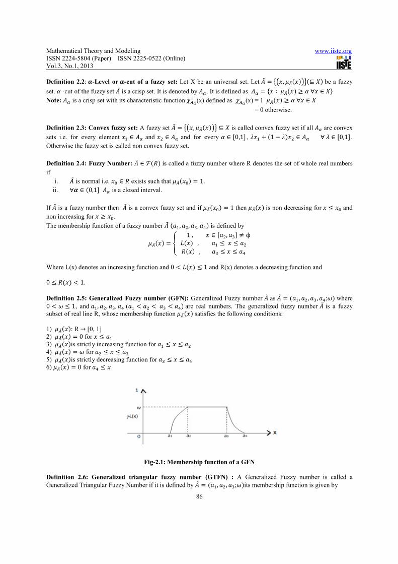
Definition 2.5: Generalized Fuzzy number (GFN): Generalized Fuzzy number � as � � �2�, 2 , 23, 24;:� where 0 9 : 1 1, and 2�, 2 , 23, 24 (2� 9 2 923 9 24�are real numbers. The generalized fuzzy number � is a fuzzy

subset of real line R, whose membership function �� satisfies the following conditions:

1) ��: R → [0, 1]

2) �� 0 for � 1 2�

3) ��is strictly increasing function for 2� 1 � 1 2

4) �� : for 2 1 � 1 23

5) ��is strictly decreasing function for 23 1 � 1 24

6) �� 0 for 24 1 �

Fig-2.1: Membership function of a GFN

Definition 2.6: Generalized triangular fuzzy number (GTFN) : A Generalized Fuzzy number is called a

Generalized Triangular Fuzzy Number if it is defined by � � �2�, 2 , 23;:�its membership function is given by



Vol.3, No.1, 2013

87

�� ;<=<> 0,� 1 2�: ?@ABAC@AB ,2� 1 � 1 2 :,� � 2 : AD@?AD@AC , 2 1 � 1 230,� & 23

or,�� E2� FEGH F: ?@ABAC@AB , :, : AD@?AD@ACI , 0I

Definition 2.7: Fuzzy ordinary differential equation (FODE):

Consider a simple 1st Order Linear non-homogeneous Ordinary Differential Equation (ODE) as

follows:

J?JK � L� - �� with initial condition �� M

The above ODE is called FODE if any one of the following three cases holds:

(i) Only M is a generalized fuzzy number (Type-I).

(ii) Only k is a generalized fuzzy number (Type-II).

(iii) Both k and M are generalized fuzzy numbers (Type-III).

Definition 2.8: Strong and Weak solution of FODE:

Consider the 1st order linear non homogeneous fuzzy ordinary differential equation

J?JK � L� - �� with �� .

Here k or (and) �� be generalized fuzzy number(s).

Let the solution of the above FODE be �N�� and its "-cut be ��, "� � ��, "�, � ��, "��. If ��, "� 1 � ��, "�∀" ∈ �0, :�where0 9 : 1 1 then �N�� is called strong solution otherwise �N�� is called

weak solution and in that case the "-cut of the solution is given by ��, "� � �min$��, "�, � ��, "�) ,max$��, "�, � ��, "�)�. 3. Solution Procedure of 1

st Order Linear Non Homogeneous FODE

The solution procedure of 1st order linear non homogeneous FODE of Type-I, Type-II and Type-III are described.

Here fuzzy numbers are taken as GTFNs.

3.1. Solution Procedure of 1st Order Linear Non Homogeneous FODE of Type-I

Consider the initial value problem J?JK � V� - �� ………….(3.1.1)

with Fuzzy Initial Condition (FIC) �N�� M�W � �M�, M , M3; :� Let �N�� be a solution of FODE (3.1.1) .

Let ��, "� � ��, "�, � ��, "�� be the "-cut of �N�� and �M�W �# � ��, "�, � ��, "�� YM� - #Z[\] , M3 . # [̂\] _∀"`�0, :�,0 9 : 1 1

where ab\ � M . M�anddb\ � M3 . M

Here we solve the given problem for L � 0 and L 9 0 respecively.



Vol.3, No.1, 2013

88

Case 3.1.1. When e � 0

The FODE (3.1.1) becomes a system of linear ODE

J?f�K,∝�JK � L�h��, "� - �� for G � 1,2 …………..(3.1.2)

with initial condition ��, "� � M� - #Z[\] and � ��, "� � M3 . # [̂\]

The solution of (3.1.2) is

��, "� � . ?\j - k?\j - �M� - #Z[\] �l mj�K@K\� ….……….(3.1.3)

and � ��, "� � . ?\j - k?\j - �M3 . # [̂\] �l mj�K@K\� . ………….(3.1.4)

Now nn# ��, "�� Z[\] mj�K@K\� � 0 , nn# �� , "�� . [̂\] mj�K@K\� 9 0

and ��, :� � . ?\j - k?\j - M l mj�K@K\� � � ��, :�. So the solution of FODE (3.1.1) is a generalized fuzzy number �N . The "-cut of the solution is

��, "� � . ?\j - Y?\j - FM� - #Z[\] I , ?\j - �M3 . # [̂\] �_ mj�K@K\�. Case 3.1.2. when e 9 0

Let L � .E where m is a positive real number.

Then the FODE (3.1.1) becomes a system of ODE as follows

pqB�r,∝�pr s@t?C�K,#�u?\pqB�r,∝�pr s@t?C�K,#�u?\v ………… …(3.1.5)

with initial condition ��, "� � M� - #Z[\] and � ��, "� � M3 . # [̂\] .

The solution of (3.1.5) is

��, "� � ?\t - � k. ?\t - M� - M3 - #] �ab\ . db\l m@t�K@K\� - � F#] . 1I �ab\ - db\mt�K@K\� and

� ��, "� � ?\t - � k. ?\t - M� - M3 - #] �ab\ . db\l m@t�K@K\� . � F#] . 1I �ab\ - db\mt�K@K\� . Here

nn# ��, "�� ] �ab\ . db\m@t�K@K\� - � ] �ab\ - db\mt�K@K\� ,

nn# �� , "�� ] �ab\ . db\m@t�K@K\� . � ] �ab\ - db\mt�K@K\�



Vol.3, No.1, 2013

89

and ��, :� � ?\t - F. ?\t - M I m@t�K@K\� � � ��, :� Here three cases arise.

Case1: When wxy �zxy i.e., xy{ � �x|, x}, x~; �� is a symmetric GTFN

∴ nn# ��, "�� ] �ab\ - db\mt�K@K\� � 0 , nn# �� , "�� . � ] �ab\ - db\mt�K@K\� 9 0

and ��, :� � � ��, :� So the solution of the FODE (3.1.1) is a strong solution.

Case2: When wxy 9zxy i.e., xy{ � �x|, x}, x~;�� is a non symmetric GTFN

Here nn# �� , "�� 9 0 and ��, :� � � ��, :� but

nn# ��, "�� 0 implies � � �� - � t log � [̂\@Z[\Z[\u [̂\�. So the solution of the FODE (3.1.1) is a strong solution if � � �� - � t log � [̂\@Z[\Z[\u [̂\�. Case3: When wxy �zxy i.e., xy{ � �x|, x}, x~;�� is a non symmetric GTFN

Here nn# ��, "�� 9 0 and ��, :� � � ��, :� but

nn# �� , "�� 9 0 implies � � �� - � t log � [̂\@Z[\Z[\u [̂\�. So the solution of the FODE (3.1.1) is a strong solution if � � �� - � t log �Z[\@ [̂\Z[\u [̂\�. 3.2. Solution Procedure of 1

st Order Linear Non Homogeneous FODE of Type-II

Consider the initial value problem J?JK � L�� - �� ………….(3.2.1)

with IC �� M . Here L� � ��, � , �3; ,�. Let �N�� be the solution of FODE (3.2.1)

Let ��, "� � ��, "�, � ��, "�� be the "-cut of the solution and the "-cut of L� be

�L�# � �L��"�, L �"�� Y�� - #Z�� , �3 . #^�� _∀"`�0, ,�,0 9 , 1 1

where aj � � . ��anddj � �3 . � .

Here we solve the given problem for L� � 0 and L� 9 0 respecively.

Case 3.2.1: when e� � 0




Vol.3, No.1, 2013

90

J?f�K,∝�JK � Lh�"��h��, ∝� - �� for G � 1,2 …………..(3.2.2)

with IC �� M .

The solution of (3.2.1)

��, "� � . ?\��Bu+�� - �M - ?\��Bu+�� v m��Bu+�� K@K\� and

� ��, "� � . ?\��D@+�� - �M - ?\��D@+�� v m��D@+�� K@K\� .

Case 3.2.2: when �� 9 0

Let L� � .EW , where EW � ��, � , �3; ,� is a positive GTFN.

So �EW�# � �E��"�,E �"�� Y�� - #Z�� , �3 . #^�� _ ∀"`�0, ,�, 0 9 , 1 1

where at � � . ��anddt � �3 . �

Then the FODE (3.2.1) becomes a system of ODE as follows

pqB�r,∝�pr s@tC�#�?C�K,#�u?\pqC�r,∝�pr s@tB�#�?B�K,#�u?\v ……………(3.2.3)

with IC �� M

Thus the solution is

��, "� �12;=

>M �1 . ��3 . "dt,�� - "at, � . ��1�� - "at, . 1�� - "at, ��3 . "dt, ��

�m��Bu#Z�� D@#^�� K@K\�

-12;=>M�1 - ��3 . "dt,�� - "at, � . ��

1�� - "at, - 1�� - "at, ��3 . "dt, ��m@�F�Bu#Z�� I��D@#^�� K@K\� - �� - "at,

� ��, "� � .12�� -

"at,�3 . "dt, ;=>M �1 . ��3 . "dt,�� - "at, � . ��

1�� - "at, . 1�� - "at, ��3 . "dt, ��m��Bu#Z�� F�D@#^�� I�K@K\�



Vol.3, No.1, 2013

91

- � ��Bu+��D@+�� 5M �1 - ��D@+��Bu+�� . �� Bu+�� - ��Bu+�� D@+�� m@�F�Bu+�� I��D@+�� K@K\� - ?\�D@+��

3.3. Solution Procedure of 1st Order Linear Non Homogeneous FODE of Type-III

Consider the initial value problem J?JK � V�� - �� ………….(3.3.1)

With fuzzy IC �N�� M�W � �M�, M , M3; :� , where L� � ��, � , �3; ,� Let �N�� be the solution of FODE (3.3.1) .

Let ��, "� � ��, "�, � ��, "�� be the "-cut of the solution.

Also �L�# � Y�� - #Z�� , �3 . #^�� _ ∀"`�0, ,�, 0 9 , 1 1

where aj � � . ��anddj � �3 . �

and �M�W �# � ��, "�, � ��, "�� YM� - #Z[\] , M3 . # [̂\] _ ∀"`�0, :�, 0 9 : 1 1

where ab\ � M . M�anddb\ � M3 . M

Let � min�,, :� Here we solve the given problem for L� � 0 and L� 9 0 respecively.

Case I: when e� � 0


J?f�K,∝�JK � Lh�h��, "� - �� for G � 1,2 …………..(3.3.2)

with initial condition ��, "� � M� - #Z[\] and � ��, "� � M3 . # [̂\]

Therefore the solution is of (3.3.1)

��, "� � . ?\��Bu+��¡ �- �FM� - #Z[\¢ I - ?\��Bu+��¡ �v mF�Bu+��¡ I�K@K\�

And

� ��, "� � . ?\��D@+��¡ �- �FM3 . # [̂\¢ I - ?\��D@+��¡ �v mF�D@+��¡ I�K@K\�

Case II: when e� 9 0

Let L� � .EW where EW � ��, � , �3; ,� is a positive GTFN.

Then �EW�# � Y�� - #Z�� , �3 . #^�� _∀"`�0, ,�,0 9 , 1 1



Vol.3, No.1, 2013

92

Let � min�,, :� Then the FODE (3.3.1) becomes a system of ODE as follows

pqB�r,∝�pr s@tC�£�?C�K,#�u?\pqC�r,∝�pr s@tB�£�?B�K,#�u?\v ………………(3.3.3)

with IC ��, "� � M� - #Z[\] and � ��, "� � M3 . # [̂\] .

Therefore the solution of (3.3.1) is

��, "� �

12;<=<>�¤�M� - "ab\ .�F�3 . "dt I

F�� - "at I �M3 . "db\ �0� �¥

�.��1F�� - "at I . 1�F�� - "at IF�3 . "dt I��<�

<�m�F�Bu#Z�¢ IF�D@#^�¢ I�K@K\�

-12;=>�M� - "ab\ -�F�3 . "dt I

F�� - "at I �M3."dM0: �� . ��1�� - "at � - 1�� - "at ��3 . "dt ��

�m@��Bu#Z�¢ ��D@#^�¢ ��K@K\� - �� - "at �

and

� ��, "� �

.12�� -"at ��3 . "dt �;=

>�M� - "ab\ . ��3 . "dt �� - "at � �M3 . "db\ �� . ��

1�� - "at � . 1�� - "at ��3 . "dt ��m��Bu#Z�¢ ��D@#^�¢ ��K@K\�

-12�� -"at ��3 . "dt �;=

>�M� - "ab\ - ��3 . "dt �� - "at � �M3 . "db\ �� . ��

1�� - "at � - 1�� - "at ��3 . "dt ��m@��Bu#Z�¢ ��D@#^�¢ ��K@K\�

- ?\��D@+��¡ � .

4. Application: Population Dynamics Model

Bacteria are being cultured for the production of medication. Without har-vesting the bacteria, the rate of change of

the population is proportional to its current population, with a proportionality constant L per hour. Also, the bacteria

are being harvested at a rate of § per hour. If there are initially �̈ bacteria in the culture, solve the initial value

problem: J©JK � L¨ . §, ¨�0� � �̈ when

(i) �̈� � �7800,8000,8150; 0.8� andL � 0.2, § � 1000,

(ii) �̈ � 8000 and L� � �0.17,0.2,0.24; 0.6�, § � 1000, (iii) �̄̈ � �7900,8000,8200; 0.7� and L� � �0.16,0.2,0.23; 0.8�, § � 1000.



Vol.3, No.1, 2013

93

Solution: (i) Here� �̈��# � �7800 - 250", 8150 . 187.5"�. Therefore solution of the model

�̈��, "� � 5000 - �2800 - 250"�m�. K and ̈��, "� � 5000 - �3150 . 187.5"�m�. K . Table-1: Value of ±|�², !� and ±}�², !� for different ! and t=3

" �̈��, "� ̈��, "� 0 10101.9326 10739.6742

0.1 10147.4856 10705.5095

0.2 10193.0386 10671.3448

0.3 10238.5916 10637.1800

0.4 10284.1445 10603.0153

0.5 10329.6975 10568.8506

0.6 10375.2505 10534.6859

0.7 10420.8034 10500.5211

0.8 10466.3564 10466.3564

From above table-1 we see that for this particular value of t=3, �̈��, "� is an increasing function, ̈��, "� is a

decreasing function and �̈��, 0.8� � ̈��, 0.8� � 10466.3564. So Solution of above model for particular value of t

is a strong solution.

(ii) Here �L��# � �0.17 - 0.050", 0.26 . 0.066"�. Therefore solution of the model is

�̈��, "� � ��.�³u�.�´�#�- k8000 . ��.�³u�.�´�#�l m��.�³u�.�´�#�K and ̈��, "� � ��. 4@�.�µµ#�- k8000 . ��. 4@�.�µµ#�l m��. 4@�.�µµ#�K.

Table-2: Value of ±|�², !� and ±}�², !� for different ! and t=3

" �̈��, "� ̈��, "� 0 9408.8519 12041.9940

0.1 9578.1917 11765.8600

0.2 9750.2390 11495.6109

0.3 9925.0361 11231.1346

0.4 10102.6256 10972.3224

0.5 10283.0510 10719.0687

0.6 10466.3564 10471.2714



Vol.3, No.1, 2013

94


decreasing function and �̈��, 0.8� 9 ̈��, 0.8�. So Solution of above model for particular value of t is a strong

solution.

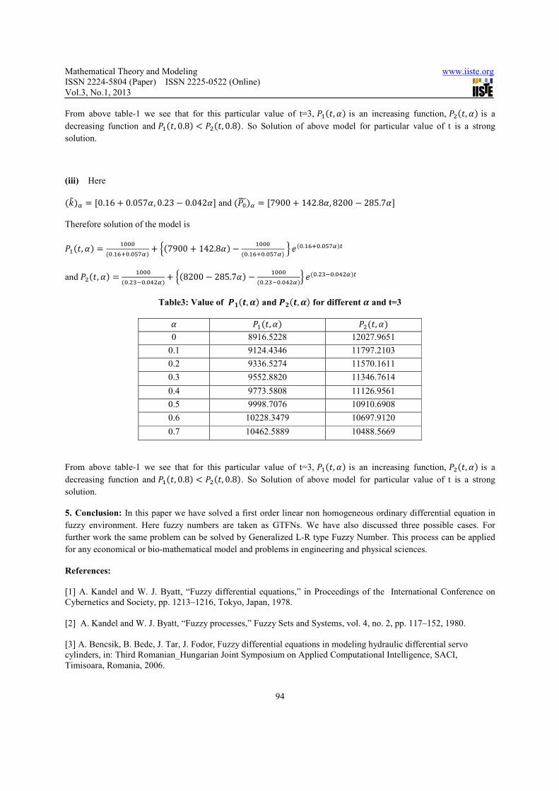
(iii) Here

�L��# � �0.16 - 0.057", 0.23 . 0.042"� and � �̄̈�# � �7900 - 142.8", 8200 . 285.7"� Therefore solution of the model is

�̈��, "� � ��.�µu�.�´³#�- k�7900 - 142.8"� . ��.�µu�.�´³#�l m��.�µu�.�´³#�K and ̈��, "� � ��. 3@�.�4 #�- k�8200 . 285.7"� . ��. 3@�.�4 #�l m��. 3@�.�4 #�K

Table3: Value of ±|�², !� and ±}�², !� for different ! and t=3

" �̈��, "� ̈��, "� 0 8916.5228 12027.9651

0.1 9124.4346 11797.2103

0.2 9336.5274 11570.1611

0.3 9552.8820 11346.7614

0.4 9773.5808 11126.9561

0.5 9998.7076 10910.6908

0.6 10228.3479 10697.9120

0.7 10462.5889 10488.5669


decreasing function and �̈��, 0.8� 9 ̈��, 0.8�. So Solution of above model for particular value of t is a strong

solution.

5. Conclusion: In this paper we have solved a first order linear non homogeneous ordinary differential equation in

fuzzy environment. Here fuzzy numbers are taken as GTFNs. We have also discussed three possible cases. For

further work the same problem can be solved by Generalized L-R type Fuzzy Number. This process can be applied

for any economical or bio-mathematical model and problems in engineering and physical sciences.

References:

[1] A. Kandel and W. J. Byatt, “Fuzzy differential equations,” in Proceedings of the International Conference on

Cybernetics and Society, pp. 1213–1216, Tokyo, Japan, 1978.

[2] A. Kandel and W. J. Byatt, “Fuzzy processes,” Fuzzy Sets and Systems, vol. 4, no. 2, pp. 117–152, 1980.

[3] A. Bencsik, B. Bede, J. Tar, J. Fodor, Fuzzy differential equations in modeling hydraulic differential servo

cylinders, in: Third Romanian_Hungarian Joint Symposium on Applied Computational Intelligence, SACI,

Timisoara, Romania, 2006.



Vol.3, No.1, 2013

95

[4] B. Bede, I.J. Rudas, A.L. Bencsik, First order linear fuzzy differential equations under generalized

differentiability, Information Sciences 177 (2007) 1648–1662.

[5] Dubois, D and H.Parade 1978, Operation on Fuzzy Number. International Journal of Fuzzy system, 9:613-626

[6] G.L. Diniz, J.F.R. Fernandes, J.F.C.A. Meyer, L.C. Barros, A fuzzy Cauchy problem modeling the decay of the

biochemical oxygen demand in water,2001 IEEE.

[7] Hassan Zarei, Ali Vahidian Kamyad, and Ali Akbar Heydari, Fuzzy Modeling and Control of HIV Infection,

Computational and Mathematical Methods in Medicine Volume 2012, Article ID 893474, 17 pages.

[8] J. J. Buckley and T. Feuring, “Fuzzy differential equations,” Fuzzy Sets and Systems, vol. 110, no. 1, pp.43–54,

2000.

[9] James J. Buckley, Thomas Feuring, Fuzzy initial value problem for Nth-order linear differential equations, Fuzzy

Sets and Systems 121 (2001) 247–255.

[10] J.J. Buckley, T. Feuring, Y. Hayashi, Linear System of first order ordinary differential equations: fuzzy initial

condition, soft computing6 (2002)415-421.

[11] L. A. Zadeh, Fuzzy sets, Information and Control, 8(1965), 338-353.

[12] L.C. Barros, R.C. Bassanezi, P.A. Tonelli, Fuzzy modelling in population dynamics, Ecol. Model. 128 (2000)

27-33.

[13] L.J. Jowers, J.J. Buckley, K.D. Reilly, Simulating continuous fuzzy systems, Information Sciences 177 (2007)

436–448.

[14] M. Oberguggenberger, S. Pittschmann, Differential equations with fuzzy parameters, Math. Modelling Syst. 5

(1999) 181-202.

[15] Muhammad Zaini Ahmad, Bernard De Baets, A Predator-Prey Model with Fuzzy Initial Populations, IFSA-

EUSFLAT 2009.

[16] O. Kaleva, Fuzzy differential equations, Fuzzy Sets and Systems 24 (1987) 301–317.

[17] S. Seikkala, On the fuzzy initial value problem, Fuzzy Sets and Systems 24 (1987) 319–330.

[18] W. Congxin, S. Shiji, Existence theorem to the Cauchy problem of fuzzy differential equations under

compactness-type conditions, Information Sciences 108 (1998) 123–134.

[19] Z. Ding, M. Ma, A. Kandel, Existence of the solutions of fuzzy differential equations with parameters,

Information Sciences 99 (1997) 205–217.

This academic article was published by The International Institute for Science,

Technology and Education (IISTE). The IISTE is a pioneer in the Open Access

Publishing service based in the U.S. and Europe. The aim of the institute is

Accelerating Global Knowledge Sharing.

More information about the publisher can be found in the IISTE’s homepage:

http://www.iiste.org

CALL FOR PAPERS

The IISTE is currently hosting more than 30 peer-reviewed academic journals and

collaborating with academic institutions around the world. There’s no deadline for

submission. Prospective authors of IISTE journals can find the submission

instruction on the following page: http://www.iiste.org/Journals/

The IISTE editorial team promises to the review and publish all the qualified

submissions in a fast manner. All the journals articles are available online to the

readers all over the world without financial, legal, or technical barriers other than

those inseparable from gaining access to the internet itself. Printed version of the

journals is also available upon request of readers and authors.

IISTE Knowledge Sharing Partners

EBSCO, Index Copernicus, Ulrich's Periodicals Directory, JournalTOCS, PKP Open

Archives Harvester, Bielefeld Academic Search Engine, Elektronische

Zeitschriftenbibliothek EZB, Open J-Gate, OCLC WorldCat, Universe Digtial

Library , NewJour, Google Scholar

http://www.iiste.org/

http://www.iiste.org/Journals/

Documents

-First Order Linear Non Homogeneous Ordinary Differential