Rapid Recovery from Robot Failures in Multi-Robot

Rapid Recovery from Robot Failuresin Multi-Robot Visibility-Based Pursuit-Evasion

Trevor Olsen, Nicholas M. Stiffler, and Jason M. O’Kane

Abstract— This paper addresses the visibility-based pursuit-evasion problem where a team of pursuer robots operating in atwo-dimensional polygonal space seek to establish visibility ofan arbitrarily fast evader. This is a computationally challengingtask for which the best known complete algorithm takes timedoubly exponential in the number of robots. However, recentadvances that utilize sampling-based methods have shownprogress in generating feasible solutions. An aspect of thisproblem that has yet to be explored concerns how to ensurethat the robots can recover from catastrophic failures whichleave one or more robots unexpectedly incapable of continuingto contribute to the pursuit of the evader. To address thisissue, we propose an algorithm that can rapidly recover fromcatastrophic failures. When such failures occur, a replanningoccurs, leveraging both the information retained from the previ-ous iteration and the partial progress of the search completedbefore the failure to generate a new motion strategy for thereduced team of pursuers. We describe an implementation ofthis algorithm and provide quantitative results that show thatthe proposed method is able to recover from robot failures morerapidly than a baseline approach that plans from scratch.

I. INTRODUCTION

For a number of important applications of mobile robots,including environmental monitoring [7], [15], [34], disasterrecovery [13], and surveillance [2], the central problem is toplan motions for a team robots called pursuers to locate un-predictably moving agents called evaders. Though progresshas been made on several forms of this problem, a keylimitation within much of the existing work is an inability toadapt in cases of unrecoverable failures of individual robots.Such failures are particularly likely to occur in the veryapplication domains for which these methods are well-suited.

Figure 1 provides a simple illustration of this problem,in a context wherein each pursuer is equipped with anomnidirectional sensor that can detect the evaders within itsline of sight. The objective is to move the pursuers alongpaths that are guaranteed to locate the evaders, even if theevaders may move arbitrarily quickly. An initial plan tosearch this environment using three robots appears on theleft of Figure 1. Now suppose the robot stationed at the topleft of the environment fails during the plan’s execution, asshown on the right of Figure 1. In this case, any evaderhiding in the center of the environment at that time can nowescape to the top left corner without being detected. Thus,the initial plan is no longer guaranteed to locate the evader.

The authors are with the Department of Computer Scienceand Engineering, University of South Carolina, Columbia, SC29208, USA. {tvolsen}@email.sc.edu {stifflen,jokane}@cse.sc.edu This material is based upon work supported bythe National Science Foundation under Grant Nos. 1659514 and 1849291.

Fig. 1: [left] An initial joint plan for 3 robots to search asimple environment for an evader. Two robots on the leftremain stationary and monitor that side of the environmentwhile a third moves to search the right. [right] The robot inthe top left corner fails unexpectedly. As a result, the initialplan is no longer correct, because it cannot locate an evaderthat moves into the top left corner of the environment.

Fig. 2: [left] The robots from Figure 1 replan, using theproposed algorithm, to form a correct plan for the remaining2 robots. [right] The plan completes successfully.

In response to this limitation, this paper proposes a newapproach for this form of visibility-based pursuit-evasionproblem, suitable for contexts in which failures of robots arelikely. Because generating pursuit plans for this domain iscomputationally challenging [29], we introduce a method forreplanning in cases of robot failure that leverages informationderived from the previous plan to accelerate the constructionof new plans for the unexpectedly-smaller teams. Figure 2shows an example of recovery from the failure depicted inFigure 1.

The central idea is to adapt known methods for solvingthese problems in the failure-free case, which are based ona roadmap-like data structure called the sample-generatedpursuit-evasion graph (SG-PEG) [30]. For planning the mo-tions of n robots in this pursuit-evasion problem, the SG-

arX

iv:2

104.

0410

9v1

[cs

.RO

] 8

Apr

202

1

PEG graph represents the connectivity of the joint configu-rations space with vertices that represent joint configurationsand edges that represent collision free movements, muchlike a traditional probabilistic roadmap. In addition, eachvertex is labeled with information that encodes which hiddenportions of the environment can be cleared of unseen evadersalong some walk in the graph ending at that vertex. Thenew replanning approach modifies this data structure when arobot fails to reflect the removal of that robot from the search.The remaining graph then provides a valuable starting pointfor the process of planning to solve the problem with theremaining n − 1 robots. The algorithm then expands thisgraph by adding additional vertices, attempting to recoverthe contributions made by the failed robot.

This work is, to the authors’ best knowledge, the firstto address the problem of recovery from pursuer failuresfor this form of pursuit-evasion problem. In the remainderof the paper, we review some related work (Section II),formally define the problem (Section III). Then we describeand evaluate the algorithm (Sections IV and V respectively)before concluding with discussion and a preview of futurework (Section VI).

II. RELATED WORK

The visibility-based pursuit-evasion problem posed in thispaper can be thought of as a specialization of the broaderproblem of search and target tracking. The common themeacross this work is the pursuit of an agent (or agents) by one(or more) pursuers to either establish or maintain visibilityof the target [27], [28], [39].

The literature on these problems can by understood byorganizing according to underlying models, including differ-ential game theory, graph variants, and geometric variants.Though this work considers the geometric formulation, wepresent a brief synopsis of the contributions in the domainsof differential game theory and graph theory.

The seminal work of Isaacs [14] and Ho et. al. [12] wasthe first to adapt the pursuit-evasion problem to a dynamicgame-theoretic framework. This remains an active researcharea [6], [18], [25], [36]. Recent results include continuedprogress by utilizing techniques such as reinforcement learn-ing [37] and the exploitation of rich representations such asVoronoi partitions to aid in the search [20], [38].

A different formulation in which the domain is modeledas a discrete graph was initially proposed by Parsons [23]and is referred to as the edge-searching problem. Petrovlater independently rediscovered some of Parsons’ results inthe context of differential game theory [24]. Golovach latershowed that both problems considered an equivalent discretegame on graphs [9]. A number of survey papers [1], [3], [5]provide overviews of the many problem variants that can berealized within the graph model, such as specifying the rulesof movement for the pursuers and for the evaders [26], thekind of graph [17], etc.

This paper specifically focuses on a variant of the problemwhere the pursuers and evaders operate in a geometricenvironment [11], [22], [33]. There are a number of results

for the single pursuer variant of the problem that range fromproviding theoretical properties such as completeness [11]and optimality [31], to more restricted scenarios where thereare limits on the actuation and sensing capabilities of thepursuers [4], [19], [32], [35]. Due to the broad range of prac-tical applications, the multi-pursuer variant of the problemhas drawn continued interest [8], [10], [16], [30] in recentyears. The multi-pursuer scenario poses additional challengesowing to the problem complexity [29]. A common threadthrough much of the existing work is an assumption thatthe pursuer(s) can reliably execute the trajectories generatedfor them by the planner. This work seeks to address thislimitation.

III. PROBLEM STATEMENT

We first define the basic problem in the absence of pursuerfailures (Section III-A) and describe how to cast that problemin terms of a discrete representation of which areas ofthe environment are ‘clear’ or ‘contaminated’ (Section III-B), before introducing the possibility of pursuer failures(Section III-C).

A. Environment, pursuers, and evaders

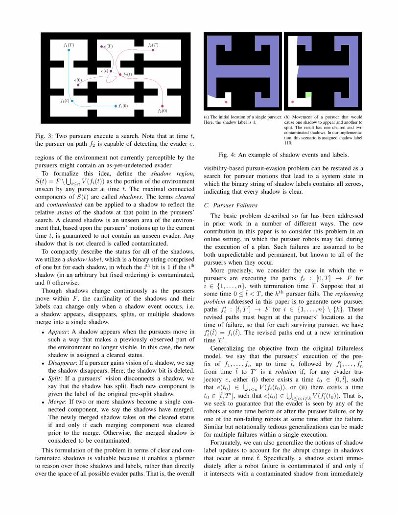
The environment F is a closed, bounded, and connectedpolygonal region in R2. A team of n pursuers, who cantravel throughout the environment at bounded speed, areequipped with omnidirectional sensors whose range is onlybounded by line of sight within the environment. That is,a pursuer at point q ∈ F can detect anything within itsvisibility polygon V (q) = {r ∈ F | qr ⊂ F}. We denotethe location of the ith pursuer as a function of the time tby the continuous function fi(t) : [0, T ] → F , in which Tis some termination time which the pursuers may choose.The n-robot joint pursuer configuration (JPC) at time t isthe vector 〈f1(t), f2(t), . . . , fn(t)〉 ∈ Fn.

A single evader seeks to avoid detection by the pursuersby moving continuously within the environment, without anybound on its speed. We denote its location, as a functionof time, by the continuous function e(t) : [0,∞) → F ,unknown to the pursuers. Observe that, because we plan forthe worst case, any strategy for the pursuers that guaranteesdetection of a single evader can also guarantee detection foreach of potentially many evaders.

The pursuers’ objective is to establish visibility withthe evader. Thus, for a given environment F , the goalis to choose the termination time T and the functionsf1, f2, . . . , fn to ensure that for any evader trajectory e, thereexists a time t0 ∈ [0, T ], such that e(t0) ∈

⋃i≤n V (fi(t0)).

Figure 3 illustrates the notation.

B. Shadows

The primary difficulty in this type of visibility-basedpursuit-evasion concerns reasoning about the regions of theenvironment that are not currently visible to the pursuers atthe present time. To resolve that difficulty, Guibas, Latombe,LaValle, Lin, and Motwani [11] introduced a reformulationof the problem, based upon tracking which, if any, of the

f1(0)f1(t)

f1(T )

f2(0)

f2(t)

f2(T )

e(0)

e(t)

e(T )

Fig. 3: Two pursuers execute a search. Note that at time t,the pursuer on path f2 is capable of detecting the evader e.

regions of the environment not currently perceptible by thepursuers might contain an as-yet-undetected evader.

To formalize this idea, define the shadow region,S(t) = F \

⋃i≤n V (fi(t)) as the portion of the environment

unseen by any pursuer at time t. The maximal connectedcomponents of S(t) are called shadows. The terms clearedand contaminated can be applied to a shadow to reflect therelative status of the shadow at that point in the pursuers’search. A cleared shadow is an unseen area of the environ-ment that, based upon the pursuers’ motions up to the currenttime t, is guaranteed to not contain an unseen evader. Anyshadow that is not cleared is called contaminated.

To compactly describe the status for all of the shadows,we utilize a shadow label, which is a binary string comprisedof one bit for each shadow, in which the ith bit is 1 if the ith

shadow (in an arbitrary but fixed ordering) is contaminated,and 0 otherwise.

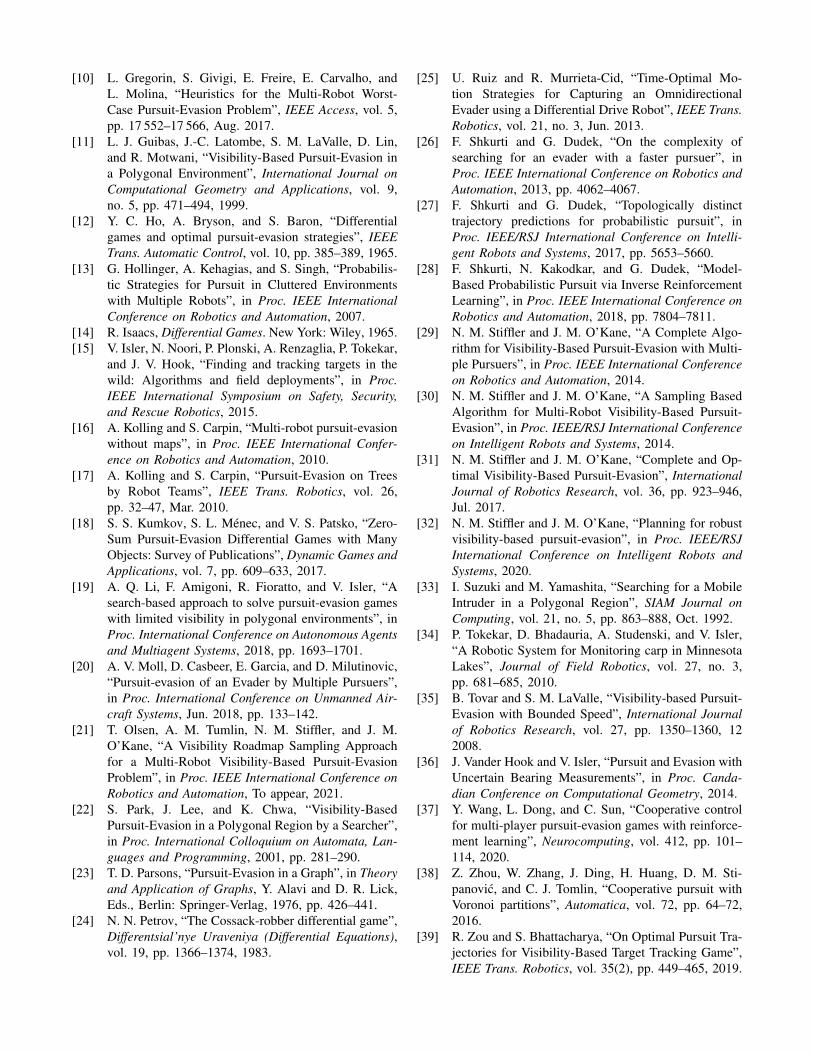
Though shadows change continuously as the pursuersmove within F , the cardinality of the shadows and theirlabels can change only when a shadow event occurs, i.e.a shadow appears, disappears, splits, or multiple shadowsmerge into a single shadow.

• Appear: A shadow appears when the pursuers move insuch a way that makes a previously observed part ofthe environment no longer visible. In this case, the newshadow is assigned a cleared status.

• Disappear: If a pursuer gains vision of a shadow, we saythe shadow disappears. Here, the shadow bit is deleted.

• Split: If a pursuers’ vision disconnects a shadow, wesay that the shadow has split. Each new component isgiven the label of the original pre-split shadow.

• Merge: If two or more shadows become a single con-nected component, we say the shadows have merged.The newly merged shadow takes on the cleared statusif and only if each merging component was clearedprior to the merge. Otherwise, the merged shadow isconsidered to be contaminated.

This formulation of the problem in terms of clear and con-taminated shadows is valuable because it enables a plannerto reason over those shadows and labels, rather than directlyover the space of all possible evader paths. That is, the overall

(a) The initial location of a single pursuer.Here, the shadow label is 1.

(b) Movement of a pursuer that wouldcause one shadow to appear and another tosplit. The result has one cleared and twocontaminated shadows. In our implementa-tion, this scenario is assigned shadow label110.

Fig. 4: An example of shadow events and labels.

visibility-based pursuit-evasion problem can be restated as asearch for pursuer motions that lead to a system state inwhich the binary string of shadow labels contains all zeroes,indicating that every shadow is clear.

C. Pursuer Failures

The basic problem described so far has been addressedin prior work in a number of different ways. The newcontribution in this paper is to consider this problem in anonline setting, in which the pursuer robots may fail duringthe execution of a plan. Such failures are assumed to beboth unpredictable and permanent, but known to all of thepursuers when they occur.

More precisely, we consider the case in which the npursuers are executing the paths fi : [0, T ] → F fori ∈ {1, . . . , n}, with termination time T . Suppose that atsome time 0 ≤ “t < T , the kth pursuer fails. The replanningproblem addressed in this paper is to generate new pursuerpaths f ′i : [“t, T ′] → F for i ∈ {1, . . . , n} \ {k}. Theserevised paths must begin at the pursuers’ locations at thetime of failure, so that for each surviving pursuer, we havef ′i(“t) = fi(“t). The revised paths end at a new terminationtime T ′.

Generalizing the objective from the original failurelessmodel, we say that the pursuers’ execution of the pre-fix of f1, . . . , fn up to time “t, followed by f ′1, . . . , f

′n

from time “t to T ′ is a solution if, for any evader tra-jectory e, either (i) there exists a time t0 ∈ [0, “t], suchthat e(t0) ∈

⋃i≤n V (fi(t0)), or (ii) there exists a time

t0 ∈ [“t, T ′], such that e(t0) ∈⋃

i≤n;i 6=k V (f ′i(t0)). That is,we seek to guarantee that the evader is seen by any of therobots at some time before or after the pursuer failure, or byone of the non-failing robots at some time after the failure.Similar but notationally tedious generalizations can be madefor multiple failures within a single execution.

Fortunately, we can also generalize the notions of shadowlabel updates to account for the abrupt change in shadowsthat occur at time “t. Specifically, a shadow extant imme-diately after a robot failure is contaminated if and only ifit intersects with a contaminated shadow from immediately

before the failure occurred. Notice, for example, in the rightportion of Figure 1, that the large shadow encompassing thecenter and upper left portion of the environment is markedcontaminated because it overlaps the central shadow whichwas contaminated before the failure. In contrast, the smallershadow in the lower right has a clear label after the failure,because the only pre-failure shadow with which it intersects(namely, itself) had a clear label. This feature of the definitionof success, which allows shadows to remain clear evenacross a failure of one of the pursuers, is crucial becauseit allows the pursuers the possibility of retaining some oftheir progress (i.e. cleared shadows) toward completing thetask, rather than starting from scratch each time.

IV. ALGORITHM OVERVIEW

This section provides a detailed description of our algo-rithm. Because no efficient algorithm for solving even thefailure-free case is known [29], we take a sampling-basedapproach. The basic idea is to construct a roadmap withinthe pursuers’ joint configuration space, using an existing datastructure called the sample-generated pursuit-evasion graph(SG-PEG), which a subset of the present authors originallyintroduced for the failure-free case [30]. We leverage thisdata structure in a new way by introducing new samplingstrategies designed to rapidly re-acquire a solution in caseswhere a pursuer must be removed.

The core of the algorithm is a method called DROPROBOTwhich, given a solution path for k robots (for some k), usesan SG-PEG to attempt to rapidly generate a solution fork − 1 robots, using the original k-robot solution as a guide.Our algorithm relies upon DROPROBOT both to generate aninitial solution for the full set of n robots —by iterativelyreducing from a rapidly-generated trivial solution— and forreplanning when a pursuer fails.

The remainder of this section presents details of themethod. After a brief review of the SG-PEG (Section IV-A), we describe the DROPROBOT method (Section IV-B)and how that method is used to generate the initial solution(Section IV-C.1) and for replanning (Section IV-C.2).

A. SG-PEG

The SG-PEG is a data structure the represents a roadmapof valid joint paths for a team of pursuers in a known envi-ronment F , augmented with information about the shadowlabels that can be achieved by executing those paths. Wepresent here a concise overview; additional detail may befound in the original paper [30].

An SG-PEG is a directed graph G = (VG, EG), inwhich one vertex v0 is designated as the root vertex. EachSG-PEG is constructed for a specific number n of pur-suers. Each vertex v ∈ VG corresponds to a specific JPC〈p1, . . . , pn〉 ∈ Fn. Each directed edge e ∈ EG connectstwo vertices v, u ∈ VG for which it is possible for everypursuer to make a collision-free straight line motion betweenthe representative configurations. That is, the existence of anedge from v to u means that, for each 1 ≤ i ≤ n, viui ⊂ F .

In addition to this graph structure, each vertex v maintainsa set of reachable shadow labels. Specifically, a shadow label` will be recorded at a particular vertex v as a reachableshadow label if there exists a walk from v0 to v that resultsin the shadow marked clear within ` indeed being clear.

The primary operation that can be performed on a SG-PEGis ADDSAMPLE(〈p1, . . . , pn〉), which accepts a collision-free JPC as input and performs the following steps:

(i) It inserts a new vertex v at the given JPC.(ii) For every existing vertex u for which the segment uv is

collision free in Fn, it adds the edges −→uv and −→vu. Theoperation then computes a mapping that describes howthe shadows at vertex u evolve as the pursuers movefrom the JPC at vertex u to the JPC at vertex v. (Theinverse mapping is applied to −→vu).

(iii) Finally, the reachable shadow label information acrossthe graph is updated by propagating the reachableshadow labels, using the mappings attached to eachedge, recursively across the graph, to determine whatnew reachable shadow labels, if any, arise due to theinclusion of the new sample v.

The SG-PEG data structure is useful for our problem be-cause, starting from a root vertex at the pursuers’ initialpositions, executing a sequence of ADDSAMPLE operationscan eventually lead to a vertex being marked with an all-zero reachable shadow label. From there, a sequence of JPCssolving the problem can readily be extracted by walkingbackward along through the graph.

B. Dropping a robot

Suppose k pursuers are at some JPC q with shadow label`, and have computed a sequence of future JPCs to visit thatwill solve the problem from that point, eventually reachingJPC with an all-clear shadow label. How can we use thisinformation to construct a new solution that can be executedfrom this point by only k − 1 of these pursuers, removingone particular pursuer from the solution? Notice that thisscenario applies both to the case of a failed pursuer (in whichcase q and ` can be derived from the current state when thefailure occurred, and ` may mark some shadows as clear) andto a complete solution starting from the pursuers’ startingposition and all-contaminated shadow label. To simplify thenotation below, we assume without loss of generality that nth

pursuer is the one removed.The DROPROBOT method, shown in Algorithm 1, solves

this problem. The algorithm constructs an SG-PEG Gk−1,starting with a root vertex at which the nth pursuer has beenremoved and the shadow label has been updated accordingly.From there, it adds a collection of junction samples, designedto recover information lost due to the removal of the nth

pursuer at each step of the existing solution. If Gk−1 doesnot contain a solution after that step, DROPROBOT continuesby inserting additional samples called web samples designedto provide good coverage, in the sense of visibility, ofthe environment. The process continues until a solution isfound, or until some arbitrary timeout expires. Details aboutjunction sampling and web sampling appear below.

Algorithm 1 DROPROBOT(F, k, q1, . . . , qm, `)

Input: An environment F ; a positive integer k; a sequenceq1, . . . , qm of k-pursuer JPCs; a shadow label ` for q1.

Output: A sequence q′1, . . . , q′m′ of (k − 1)-pursuer JPCs

leading to an all clear shadow label at q′m′ or FAILED.1: Gk−1 ← new SG-PEG for k − 1 pursuers2: 〈p1, . . . , pk〉 ← q13: r ← Gk−1.ADDROOT(〈p1, . . . , pk−1〉)4: `′ ← ` updated for the removal of pn5: r.ADDREACHABLE(`′)6: for i← 1, . . . ,m do7: ADDJUNCTIONSAMPLES(k, Gk−1, qi)8: while Gk−1 has no solution and time remains do9: q ← WEBSAMPLE(Gk−1)

10: G.ADDSAMPLE(q)

11: if Gk−1 has a solution then12: return Gk−1.EXTRACTSOLUTION()13: else14: return FAILED

Algorithm 2 ADDJUNCTIONSAMPLES(k, Gk−1, q)

Input: A positive integer k; an SG-PEG Gk−1 for k − 1pursuers; a k-pursuer JPC q

Output: No return value, but samples are added to Gk−1.1: 〈p1, . . . , pk〉 ← q2: Gk−1.ADDSAMPLE(〈p1, . . . , pn−1〉)3: for i← 1, . . . , n− 1 do4: if V (pi) ∩ V (pn) 6= ∅ then5: z ← random point in V (pi) ∩ V (pn)6: G.ADDSAMPLE(〈p1, p2, . . . , z, . . . , pn−1〉)7: G.ADDSAMPLE(〈p1, p2, . . . , pn, . . . , pn−1〉)

1) Junction sampling: The objective in junction samplingis, informally, to add vertices and edges to the SG-PEG thatallow remaining pursuers to ‘fill in’ for the removed robot,wherever possible. Figure 5 shows a simple example of apursuer removed from a JPC during DROPROBOT. In thisexample, the lower pursuer is removed, leaving the bottomportion of the environment unobserved. Junction samplingadds new samples that provide a path within the SG-PEGfor the rightmost robot to visit the site of this lower portion.

This process, called ADDJUNCTIONSAMPLES, is formal-ized in Algorithm 2. In the general case, the algorithmidentifies a remaining pursuer at a position pi for whichthe visibility polygon intersects the visibility polygon of theposition pn of the removed pursuer. When this relationshipis detected, we add a sample that places the ith pursuer inthe intersection of the visibility polygons (see Figure 5c) andanother that places the ith pursuer at the former location ofthe nth pursuer (Figure 5d). This process is repeated for eachi and, via repeated calls to ADDJUNCTIONSAMPLES, eachstep of the previous k-pursuer solution.

2) Web sampling: Though the structures introduced byjunction sampling may be sufficient to build a SG-PEG thatcan generate a solution with k − 1 pursuers, such successcannot be guaranteed. Therefore, after exhausting the junc-

(a) The initial JCP. The nth pursuer is blue[bottom], and the ith pursuer is red [right].

(b) The first sample to be added. The nth

pursuer is removed (Algorithm 2, line 2).tructed

(c) The second sample. The nth pursueris removed and the ith pursuer movesto a random point in V (pi) ∩ V (pn).(Algorithm 2, line 6).

(d) The third sample. The nth pursuer isremoved and the ith pursuer takes its place.(Algorithm 2, line 7).

Fig. 5: An example of junction sampling.

(a) A set of 35 samples that form onecomplete web.

(b) 25000 samples drawn using web sam-pling. Notice how the points from A (red)are biased towards the outer hooks, whilethe points from B (blue) favor the regionsconnecting adjacent hooks.

Fig. 6: An illustration of web sampling.

tion samples, Algorithm 1 continues with a broader samplingstrategy called web sampling. Web sampling was originallyproposed for the failure-free version of the problem [21].

The sampling approach is based on an underlying notion ofa web. The intuition is select a collection of positions that cansee the entire environment while also forming a connectedgraph via straight-line connections within F . Generatinga web occurs in two stages. First, we draw a collectionof points A = {a1, a2, . . . , an} ⊂ F which provide fullvisibility of the environment, i.e.

⋃1≤i≤n V (ai) = F . This

is done incrementally, by drawing samples from the unseenportion if F until all of F is seen by some point in A. Thesecond stage generates an intersection set B as follows. Foreach pair of distinct points ai, aj ∈ A, if V (ai)∩V (aj) 6= ∅,we add a point b ∈ V (ai) ∩ V (aj) to B. The combinationA∪B forms one complete web; those points are utilized in

a randomly shuffled order. See Figure 6.To use these webs within WEBSAMPLE (recall line 9 in

Algorithm 1), we generate one web for each of the k − 1pursuers. Then select a random vertex v from Gk−1 and,for two of the robots in that JPC, form a new sampleby replacing the existing positions with positions drawn(without replacement) from those pursuers’ respective webs.If any web ever has no more points to choose from, wegenerate new webs for each pursuer and continue the process.

C. Planning, execution, and replanning

Armed with the DROPROBOT method, we can considerhow to use that algorithm for the overall problem.

1) Generating the initial solution: To begin, we mustgenerate an initial solution that the full complement of nrobots can begin to execute. First, we generate a trivialsolution, namely a strategy where no movement is requiredby the pursuers because their visibility polygons fully coverthe environment. We do so by iteratively adding pursuersat random unseen locations until no shadows remain. Thissingle JPC becomes our trivial solution.

Note, however —recalling that only n robots are availableat the start—, that it is rather likely that the trivial solutionwill require more than n robots. If so, we repeatedly applyDROPROBOT, selecting the pursuer to remove at random,until a solution requiring only n pursuers has been formed.The pursuer team then begins to execute this strategy.1

2) Replanning after pursuer failures: If, during the ex-ecution of the search, a pursuer fails for some reason, areplanning operation is required. In that case, we pause thepursuers’ movement until a new solution with one fewerpursuer is generated. This new solution may be generateddirectly by DROPROBOT. Notice that the inputs to thatalgorithm include the current state of the search (includingthe current JPC and the current shadow label), which areleveraged to replan more rapidly than planning from scratcheach time. Once a new solution is computed, the pursuersresume their search.

V. EVALUATION

We implemented our algorithm in C++ and executed thecode on an Ubuntu 20.04 laptop equipped with an Intel i7-10510U CPU and 16GB of RAM.

An example execution is illustrated in Figure 7. First, aninitial solution is generated (Figure 7a). Next, Figures 7b,crepresent the input and output of Algorithm 1 when the greenpursuer malfunctions. Similarly, Figures 7d,e show the statebefore and after the failure of the orange pursuer.

We simulated teams initially consisting of n = 5 pursuers2

1It is possible in principle that the trivial solution may require n robotsor less. In that case, we can ignore any additional robots beyond the m thatare required for the trivial solution and simply ‘execute’ the trivial solution.

2Increasing n has a positive effect on the planning time of the proposedalgorithm, since, by construction, we need to generate solutions for eachnumber of pursuers between the number of pursuer in the trivial solutionand n. In contrast, OTSO21 can struggle with larger values of n due tothe increased complexity of the joint configuration space, making it moredifficult to connect pursuer configurations. Thus, we hold n fixed at 5 toenable a fair comparison.

in three different environments, depicted in Figures 3, 4, and6. These environments were selected because they highlightseveral interesting attributes, such as hard to reach corners,narrow corridors, and evenly spaced obstacles. Additionally,these environments allow us to more directly compare againstexisting results. In particular, we compare the algorithmpresented in Section IV (‘this paper’) against our previousalgorithm [21] (‘OTSO21’), which was designed for thefailure-free setting, as a baseline. During each execution, wesimulated m pursuer failures. For each failure, a randomly-selected pursuer was removed when the pursuers had com-pleted a percentage β of their planned paths. For OTSO21,the algorithm was executed from scratch for the initialsolution and at each robot failure. Runs were conducted forall four combinations of m ∈ {2, 3} and β ∈ {30%, 70%}.

Each trial was limited to at most 10 minutes of run time,including both planning time and (simulated) execution time.If, after that time, the robots had not yet successfully clearedall shadows, the simulation would have been considered afailure. In the results presented here, none of the trials failed.

For each combination of environment, algorithm, team sizen, number of failures m, and failure time β, we conducted 25trials. The success or failure of the run and total computationtime spent planning and replanning were recorded. Planningtime is summarized by the mean (µ) and the standarddeviation (σ) over all trials. Tables I and II report the results,from which a few conclusions may be drawn.

Replanning is beneficial Recall from Section IV-B.1 thatjunction sampling was developed to “recover” informationin the event of a pursuer failure. The notable improvementsfor the proposed algorithm compared to OTSO21 in theenvironments of Figure 3 and Figure 4 can be attributedto efficiencies gained by re-planning rather than startingfrom scratch. In the environment of Figure 6, the proposedalgorithm performed similarly to OTSO21, likely due to thecomplexity of the environment resulting in a high number ofpursuers in its trivial solutions and subsequently more callsto DROPROBOT to reach the initial solution.

Later failures are easier to recover For the trials withβ = 70%, the total planning time was less than whenβ = 30%. This is likely due to the fact that allowingmore time to traverse the solution path will, in many cases,provide the next planning stage with an improved shadowlabel (i.e. more cleared shadows), reducing the difficulty ofthe replanning problem.

Impacts of the number of failures Increasing from m = 2to m = 3 increased the planning time for both algorithms.We speculate that this can be attributed to the additionalpursuer failure for which both the proposed algorithm andOTSO21 are required to recompute strategies.

VI. CONCLUSION

We presented a method of deconstructing higher dimen-sional solutions in order to alleviate the issue of potential

(a) An initial solution with 5 pur-suers.

(b) The problem state right beforethe green pursuer fails.

(c) The new solution paths gener-ated after the green pursuer fails.

(d) The problem state right beforethe orange pursuer fails.

(e) The new solution paths gener-ated after the orange pursuer fails.

Fig. 7: Snapshots of our algorithm through a single successful execution (n = 5,m = 2).

Table I: Simulation results for n = 5 initial pursuers andm = 2 failures. success planning time (s)

rate µ σFigure 3

This paper (β = 30%) 100% 46.09 21.50OTSO21 (β = 30%) 100% 99.57 65.03This paper (β = 70%) 100% 32.46 14.84OTSO21 (β = 70%) 100% 89.36 59.62

Figure 4This paper (β = 30%) 100% 6.47 7.46OTSO21 (β = 30%) 100% 56.13 17.20This paper (β = 70%) 100% 5.07 5.97OTSO21 (β = 70%) 100% 52.87 17.59


robotic failures in a visibility-based pursuit-evasion problem.We did this by building a new sampling strategy whichallowed us to utilize previously computed information. Ouralgorithm was able to greatly our-perform existing algorithmsin the context of our problem. Future work could includegenerating solutions that are intentionally robust to failures.That is, a solution that would still be a solution if a limitednumber of pursuers were to completely malfunction. Onepossible approach to this problem would be to expand theshadow labels from single clear/contaminated bits, to a richerrepresentation of the sets of pursuer failures under which thatshadow would nonetheless be clear.

REFERENCES

[1] T. V. Abramovskaya and N. N. Petrov, “The theory ofguaranteed search on graphs”, Vestnik St. PetersburgUniversity, vol. 46, no. 2, pp. 49–75, 2013.

[2] J. J. Acevedo, B. C. Arrue, I. Maza, and A. Ollero, “ADecentralized Algorithm for Area Surveillance Mis-sions Using a Team of Aerial Robots with DifferentSensing Capabilities”, in Proc. IEEE InternationalConference on Robotics and Automation, 2014.

[3] B. Alspach, “Searching and sweeping graphs: a briefsurvey”, Matematiche, vol. 59, pp. 5–37, 2004.

Table II: Simulation results for n = 5 initial pursuers andm = 3 failures. success planning time (s)

rate µ σFigure 3

This paper (β = 30%) 100% 63.92 29.89OTSO21 (β = 30%) 100% 117.90 64.78This paper (β = 70%) 100% 39.88 20.61OTSO21 (β = 70%) 100% 102.57 63.03



[4] D. Bhadauria, K. Klein, V. Isler, and S. Suri, “Cap-turing an Evader in Polygonal Environments withObstacles: The Full Visibility Case”, InternationalJournal of Robotics Research, vol. 31, pp. 1176–1189,10 2012.

[5] R. Borie, S. Koenig, and C. Tovey, “Pursuit-EvasionProblems”, in Handbook of Graph Theory, J. Gross, J.Yellen, and P. Zhang, Eds., Chapman and Hall, 2013,ch. 9.5, pp. 1145–1165.

[6] J. Chen, W. Zha, Z. Peng, and D. Gu, “Multi-playerpursuit–evasion games with one superior evader”, Au-tomatica, vol. 71, pp. 24–32, 2016.

[7] P. Dames, P. Tokekar, and V. Kumar, “Detecting, lo-calizing, and tracking an unknown number of movingtargets using a team of mobile robots”, InternationalJournal of Robotics Research, vol. 36, no. 13-14,pp. 1540–1553, 2017.

[8] J. W. Durham, A. Franchi, and F. Bullo, “Distributedpursuit-evasion without mapping or global localiza-tion via local frontiers”, Autonomous Robots, vol. 32,pp. 81–95, 2012.

[9] P. Golovach, “A Topological Invariant in PursuitProblems”, Differentsial’nye Uraveniya (DifferentialEquations), vol. 25, pp. 923–929, 1989.

[10] L. Gregorin, S. Givigi, E. Freire, E. Carvalho, andL. Molina, “Heuristics for the Multi-Robot Worst-Case Pursuit-Evasion Problem”, IEEE Access, vol. 5,pp. 17 552–17 566, Aug. 2017.

[11] L. J. Guibas, J.-C. Latombe, S. M. LaValle, D. Lin,and R. Motwani, “Visibility-Based Pursuit-Evasion ina Polygonal Environment”, International Journal onComputational Geometry and Applications, vol. 9,no. 5, pp. 471–494, 1999.

[12] Y. C. Ho, A. Bryson, and S. Baron, “Differentialgames and optimal pursuit-evasion strategies”, IEEETrans. Automatic Control, vol. 10, pp. 385–389, 1965.

[13] G. Hollinger, A. Kehagias, and S. Singh, “Probabilis-tic Strategies for Pursuit in Cluttered Environmentswith Multiple Robots”, in Proc. IEEE InternationalConference on Robotics and Automation, 2007.

[14] R. Isaacs, Differential Games. New York: Wiley, 1965.[15] V. Isler, N. Noori, P. Plonski, A. Renzaglia, P. Tokekar,

and J. V. Hook, “Finding and tracking targets in thewild: Algorithms and field deployments”, in Proc.IEEE International Symposium on Safety, Security,and Rescue Robotics, 2015.

[16] A. Kolling and S. Carpin, “Multi-robot pursuit-evasionwithout maps”, in Proc. IEEE International Confer-ence on Robotics and Automation, 2010.

[17] A. Kolling and S. Carpin, “Pursuit-Evasion on Treesby Robot Teams”, IEEE Trans. Robotics, vol. 26,pp. 32–47, Mar. 2010.

[18] S. S. Kumkov, S. L. Ménec, and V. S. Patsko, “Zero-Sum Pursuit-Evasion Differential Games with ManyObjects: Survey of Publications”, Dynamic Games andApplications, vol. 7, pp. 609–633, 2017.

[19] A. Q. Li, F. Amigoni, R. Fioratto, and V. Isler, “Asearch-based approach to solve pursuit-evasion gameswith limited visibility in polygonal environments”, inProc. International Conference on Autonomous Agentsand Multiagent Systems, 2018, pp. 1693–1701.

[20] A. V. Moll, D. Casbeer, E. Garcia, and D. Milutinovic,“Pursuit-evasion of an Evader by Multiple Pursuers”,in Proc. International Conference on Unmanned Air-craft Systems, Jun. 2018, pp. 133–142.

[21] T. Olsen, A. M. Tumlin, N. M. Stiffler, and J. M.O’Kane, “A Visibility Roadmap Sampling Approachfor a Multi-Robot Visibility-Based Pursuit-EvasionProblem”, in Proc. IEEE International Conference onRobotics and Automation, To appear, 2021.

[22] S. Park, J. Lee, and K. Chwa, “Visibility-BasedPursuit-Evasion in a Polygonal Region by a Searcher”,in Proc. International Colloquium on Automata, Lan-guages and Programming, 2001, pp. 281–290.

[23] T. D. Parsons, “Pursuit-Evasion in a Graph”, in Theoryand Application of Graphs, Y. Alavi and D. R. Lick,Eds., Berlin: Springer-Verlag, 1976, pp. 426–441.

[24] N. N. Petrov, “The Cossack-robber differential game”,Differentsial’nye Uraveniya (Differential Equations),vol. 19, pp. 1366–1374, 1983.

[25] U. Ruiz and R. Murrieta-Cid, “Time-Optimal Mo-tion Strategies for Capturing an OmnidirectionalEvader using a Differential Drive Robot”, IEEE Trans.Robotics, vol. 21, no. 3, Jun. 2013.

[26] F. Shkurti and G. Dudek, “On the complexity ofsearching for an evader with a faster pursuer”, inProc. IEEE International Conference on Robotics andAutomation, 2013, pp. 4062–4067.

[27] F. Shkurti and G. Dudek, “Topologically distincttrajectory predictions for probabilistic pursuit”, inProc. IEEE/RSJ International Conference on Intelli-gent Robots and Systems, 2017, pp. 5653–5660.

[28] F. Shkurti, N. Kakodkar, and G. Dudek, “Model-Based Probabilistic Pursuit via Inverse ReinforcementLearning”, in Proc. IEEE International Conference onRobotics and Automation, 2018, pp. 7804–7811.

[29] N. M. Stiffler and J. M. O’Kane, “A Complete Algo-rithm for Visibility-Based Pursuit-Evasion with Multi-ple Pursuers”, in Proc. IEEE International Conferenceon Robotics and Automation, 2014.

[30] N. M. Stiffler and J. M. O’Kane, “A Sampling BasedAlgorithm for Multi-Robot Visibility-Based Pursuit-Evasion”, in Proc. IEEE/RSJ International Conferenceon Intelligent Robots and Systems, 2014.

[31] N. M. Stiffler and J. M. O’Kane, “Complete and Op-timal Visibility-Based Pursuit-Evasion”, InternationalJournal of Robotics Research, vol. 36, pp. 923–946,Jul. 2017.

[32] N. M. Stiffler and J. M. O’Kane, “Planning for robustvisibility-based pursuit-evasion”, in Proc. IEEE/RSJInternational Conference on Intelligent Robots andSystems, 2020.

[33] I. Suzuki and M. Yamashita, “Searching for a MobileIntruder in a Polygonal Region”, SIAM Journal onComputing, vol. 21, no. 5, pp. 863–888, Oct. 1992.

[34] P. Tokekar, D. Bhadauria, A. Studenski, and V. Isler,“A Robotic System for Monitoring carp in MinnesotaLakes”, Journal of Field Robotics, vol. 27, no. 3,pp. 681–685, 2010.

[35] B. Tovar and S. M. LaValle, “Visibility-based Pursuit-Evasion with Bounded Speed”, International Journalof Robotics Research, vol. 27, pp. 1350–1360, 122008.

[36] J. Vander Hook and V. Isler, “Pursuit and Evasion withUncertain Bearing Measurements”, in Proc. Canda-dian Conference on Computational Geometry, 2014.

[37] Y. Wang, L. Dong, and C. Sun, “Cooperative controlfor multi-player pursuit-evasion games with reinforce-ment learning”, Neurocomputing, vol. 412, pp. 101–114, 2020.

[38] Z. Zhou, W. Zhang, J. Ding, H. Huang, D. M. Sti-panovic, and C. J. Tomlin, “Cooperative pursuit withVoronoi partitions”, Automatica, vol. 72, pp. 64–72,2016.

[39] R. Zou and S. Bhattacharya, “On Optimal Pursuit Tra-jectories for Visibility-Based Target Tracking Game”,IEEE Trans. Robotics, vol. 35(2), pp. 449–465, 2019.

Documents

Rapid Recovery from Robot Failures in Multi-Robot