LUND UNIVERSITY

PO Box 117221 00 Lund+46 46-222 00 00

Rao-Blackwellized Auxiliary Particle Filters for Mixed Linear/Nonlinear Gaussianmodels

Nordh, Jerker

Published in:[Host publication title missing]

Published: 2014-01-01

Link to publication

Citation for published version (APA):Nordh, J. (2014). Rao-Blackwellized Auxiliary Particle Filters for Mixed Linear/Nonlinear Gaussian models. In[Host publication title missing] (pp. 1-6). IEEE--Institute of Electrical and Electronics Engineers Inc..

General rightsCopyright and moral rights for the publications made accessible in the public portal are retained by the authorsand/or other copyright owners and it is a condition of accessing publications that users recognise and abide by thelegal requirements associated with these rights.

• Users may download and print one copy of any publication from the public portal for the purpose of privatestudy or research. • You may not further distribute the material or use it for any profit-making activity or commercial gain • You may freely distribute the URL identifying the publication in the public portal

Take down policyIf you believe that this document breaches copyright please contact us providing details, and we will removeaccess to the work immediately and investigate your claim.

Download date: 11. Jul. 2018

Rao-Blackwellized Auxiliary Particle Filters for

Mixed Linear/Nonlinear Gaussian models

Jerker Nordh

Department of Automatic Control

Lund University, Sweden

Email: jerker.nordh@control.lth.se

Abstract—The Auxiliary Particle Filter is a variant of thecommon particle filter which attempts to incorporate informationfrom the next measurement to improve the proposal distributionin the update step. This paper studies how this can be donefor Mixed Linear/Nonlinear Gaussian models, it builds on apreviously suggested method and introduces two new variantswhich tries to improve the performance by using a more detailedapproximation of the true probability density function whenevaluating the so called first stage weights. These algorithms arecompared for a couple of models to illustrate their strengths andweaknesses.

I. INTRODUCTION

The particle filter (PF) [1][2][3] has become one of thestandard algorithms for nonlinear estimation and has proved itsusefulness in a wide variety of applications. It is an applicationof the general concept of Sequential Importance Resampling(SIR)[4]. At each time the true probability density function isapproximated by a number of point estimates, the so calledparticles. These are propagated forward in time using thesystem dynamics. For each measurement the weight of eachparticle is updated with the corresponding likelihood of themeasurement. The last step is to resample the particles, thisoccurs either deterministically or only when some criteria isfulfilled. This criteria is typically the so called number ofeffective particles, which is a measure of how evenly theweights are distributed among the particles. The resamplingis a process that creates a new set particles where all particleshave equal weights, which is accomplished by drawing themwith probability corresponding to their weight in the originalset. This process is needed since otherwise eventually all theweights except one would go to zero. The resampling thusimproves the estimate by focusing the particles to regions withhigher probability.

The Auxiliary Particle Filter (APF)[5][6][7] attempts toimprove this by resampling the particles at time t using thepredicted likelihood of the measurement at time t + 1. Ifdone properly this helps to focus the particles to areas wherethe measurement has a high likelihood. The problem is thatit requires the evaluation of the probability density functionp(yt+1|xt). This is typically not available and is therefore oftenapproximated by assuming that next state is the predicted meanstate, i.e. xt+1 = xt+1|t and the needed likelihood insteadbecomes p(yt+1|xt+1 = xt+1|t).

This paper focuses on the special case of Mixed Lin-ear/Nonlinear Gaussian (MLNLG) models, which is a specialcase of Rao-Blackwellied models. For an introduction to theRao-Blackwellized Particle Filter see [8]. Rao-Blackwellized

models have the property that conditioned on the nonlinearstates there exists a linear Gaussian substructure that can beoptimally estimated using a Kalman filter. This reduces thedimensionality of the model that the particle filter should solve,thereby reducing the complexity of the estimation problem.The general form for MLNLG models is shown in (1), wherethe state vector has been split in two parts, x = (ξ z)T . Hereξ are the nonlinear states that are estimated by the particlefilter, z are the states that conditioned on the trajectory ξ1:tare estimated using a Kalman filter.

ξt+1 = fξ(ξt) +Aξ(ξt)zt + vξ (1a)

zt+1 = fz(ξt) +Az(ξt)zt + vz (1b)

yt+1 = g(ξt+1) + C(ξt+1)zt+1 + e (1c)(

vξvz

)

∼ N

(

0,

(

Qξ(ξt) Qξz(ξt)Qzξ(ξt) Qz(ξt)

))

(1d)

e ∼ N(0, R(ξt)) (1e)

In [9] an approximation is presented that can be usedwith the APF for this type of models, section II presentsthat algorithm and two variants proposed by the author ofthis paper. Section III compares the different algorithms byapplying them to a number of examples to highlight theirstrengths and weaknesses. Finally section IV concludes thepaper with some discussion of the trade-offs when choosingone of theses algorithms.

II. ALGORITHMS

A. Auxiliary Particle Filter introduction

xt+1 = f(xt, vt) (2a)

yt = h(xt, et) (2b)

Looking at a generic state-space model of the form in (2)and assuming we have a collection of weighted point estimates(particles) approximating the probability density function of

xt|t ≈ ∑N

i=1 w(i)δ(xt − x

(i)t ) the standard particle filter can

be summarized in the following steps that are done for eachtime instant t.

1) (Resample; draw N new samples x(i)t from the

categorical distribution over x(i)t with probabilities

proportional to w(i)t . Set w

(i)t = 1

N.)

2) For all i; sample v(i)t from the noise distribution

3) For all i; calculate x(i)t+1|t = f(x

(i)t , v

(i)t )

4) For all i; calculate w(i)t+1 = w

(i)t p(yt|x(i)

t+1|t)

The resampling step introduces variance in the estimate, butis necessary for the long term convergence of the filter. Step1 is therefore typically not done at each time instant but onlywhen a prespecified criteria on the weights are fulfilled.

The Auxiliary Particle Filter introduces an additional stepto incorporate knowledge of the future measurement yt+1

before updating the point estimates x(i)t .

1) For all i; calculate w(i)t = l(i)w

(i)t , where l(i) =

p(yt+1|x(i)t )

2) (Resample; draw N new samples x(i)t from the

categorical distribution over x(i)t with probabilities

proportional to l(i)w(i)t . Set wt =

1N

.)

3) For all i; sample from v(i)t from the noise distribution

4) For all i; calculate x(i)t+1|t = f(x

(i)t , v

(i)t )

5) For all i; calculate w(i)t+1 =

w(i)t

l(i)p(yt|x(i)

t+1|t)

The difference between the algorithms in the rest of sectionII is in how the first stage weights, l(i), are approximated forthe specific class of model (1).

B. Algorithm 1

The first algorithm considered is the one presented in[9]. It computes p(yt+1|xt) using the approximate modelshown in (3). This approximation ignores the uncertainty inthe measurement that is introduced through the uncertaintyin ξt+1, thereby underestimating the total uncertainty in themeasurement. Tbjs could lead to resampling of the particleseven when the true particle weights would not indicate the needfor resampling. Here Pzt denotes the estimated covariancefor the variable zt. In (3e) the dependence on ξt has beensuppressed to not clutter the notation.

p(yt+1|xt) ∼ N(yt+1, Pyt+1) (3a)

ξt+1 = fξ(ξt) +Aξ(ξt)zt (3b)

zt+1 = fz(ξt) +Az(ξt)zt (3c)

yt+1 = g(ξt+1) + C(ξt+1)zt+1 (3d)

Pyt+1 ≈ C(AzPztATz +Q)CT +R (3e)

C. Algorithm 2

Our first proposed improvement to the algorithm in sectionII-B is to attempt to incorporate the uncertainty of ξt+1 inour measurement by linearizing the measurement equationaround the predicted mean. For the case when C and R hasno dependence on ξ the pdf of the measurement can then beapproximated in the same way, except for Pyt+1 which insteadis approximated according to (4), here Jg is Jacobian of g. Thedifference compared to model 1 lies in the additional terms forthe covariance Pyt+1 due propagating the uncertainty of ξt+1

by using the Jacobian of g.

Pyt+1 ≈ (JgAξ + CAz)Pzt(JgAξ + CAz)T

+ (Jg + C)Q(Jq + C)T +R (4)

D. Algorithm 3

If the linearization scheme presented in Section II-C is towork well g must be close to linear in the region where ξt+1

has high probability. Another commonly used approximationwhen working with Gaussian distributions and nonlinearities isthe Unscented Transform used in e.g. the Unscented KalmanFilter[10]. The second proposed algorithms uses the UT toapproximate the likelihood of the measurement. It propagatesa set of so called Sigma-point through both the time update (2a)and the measurement equation (2b) and estimates the resultingmean and covariance of the points after the transformations.This is then used as the approximation for yt+1 and Pyt+1 . Thisavoids the need to linearize the model, and can thus handlediscontinuities and other situations where linearization cannotbe used or gives a poor approximation.

The Sigma-points, x(i)σ , were chosen according to (5), using

twice the number of points as the combined dimension of thestate and noise vectors (Nx). Σx is the combined covariancematrix. (

√NxΣx)i is the i-th column of R, where NxΣx =

RRT . All the points were equally weighted. This conforms tothe method introduced in section III-A in [10].

Σx = diag(Pzt , Q, R) (5a)

W (i) = (2Nx)−1, i ∈ 1..2Nx (5b)

x(i)σ = x+ (

√

NxΣx)i, i ∈ 1..Nx (5c)

x(i+Nx)σ = x− (

√

NxΣx)i, i ∈ 1..Nx (5d)

III. RESULTS

To study the difference in performance of the three algo-rithms we will look at two models, the first one was introcudedin [11] and is an extension of a popular nonlinear model toinclude a linear Gaussian substructure. The second model wasdesigned to highlight problems with the approximation usedin Algorithm 1.

A. Model 1

ξt+1 =ξt

1 + ξ2t( 0 0.04 0.044 0.008 ) zt +

+ 0.5ξt + 25ξt

1 + ξ2t+ 8 cos 1.2t+ vξ,t (6a)

zt+1 =

3 −1.691 0.849 −0.32012 0 0 00 1 0 00 0 0.5 0

zt +

+ vz,t (6b)

yt = 0.05ξ2t + et (6c)

ξ0 = 0, z0 = ( 0 0 0 0 )T

(6d)

R = 0.1, Qξ = 0.005 (6e)

Qz = diag(0.01 0.01 0.01 0.01) (6f)

Notice the square in the measurement equation in (6c),depending on the magnitude of uncertainty in ξt a linearizionof this term might lead to a poor approximation. So wemight expect that for this model the unscented transform basedapproximation might fare better.

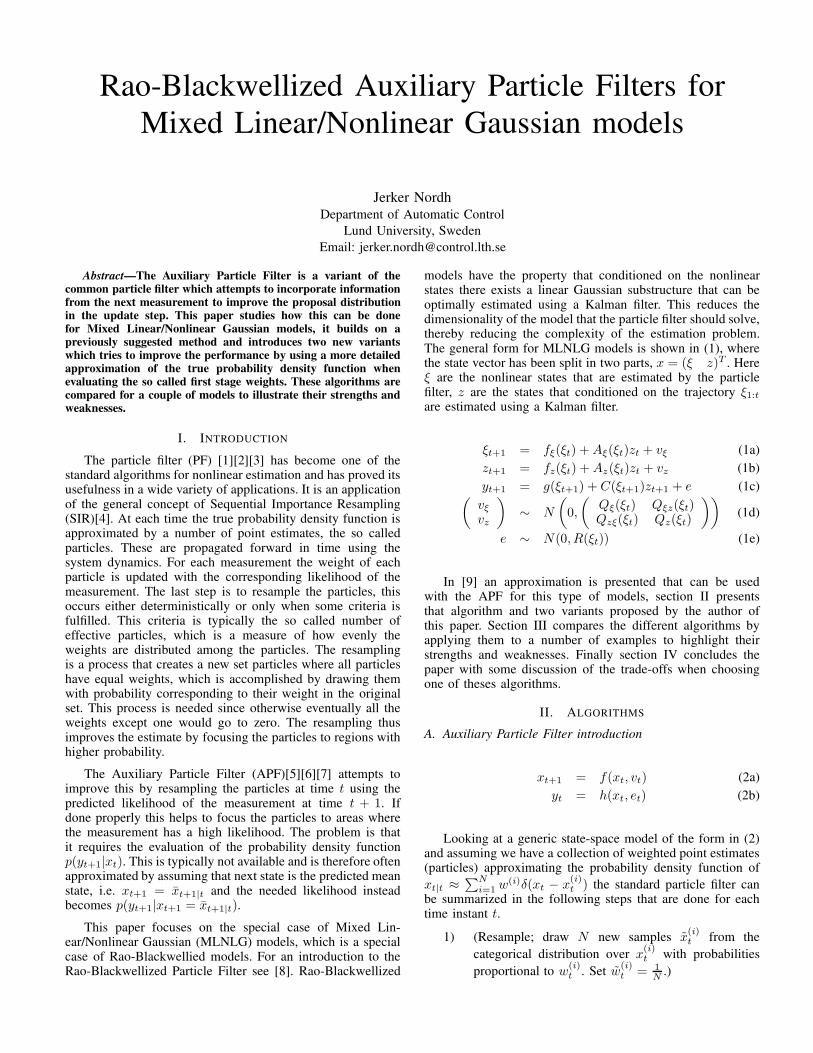
The performance of the algorithms was tested by generat-ing 25000 dataset from (6), all the algorithms were then testedon this collection for a number of different particle counts.The average RMSE values are presented in table I, they arealso shown in Fig. 1. The relative RMSE of the algorithmscompared to the standard particle filter is shown in Table II.As can be seen both algorithm 2 and 3 outperform Algorithm1, most of the time Algorithm 3 also beats Algorithm 2. Thisis expected since they use a more detailed approximation ofthe true density of p(yt+1|xt).

N PF Alg. 1 Alg. 2 Alg. 3

10 1.701 1.611 1.607 1.600

15 1.395 1.338 1.322 1.322

20 1.234 1.170 1.153 1.154

25 1.121 1.061 1.060 1.052

30 1.049 0.992 0.978 0.978

40 0.955 0.893 0.885 0.880

50 0.874 0.831 0.824 0.819

75 0.782 0.737 0.732 0.730

100 0.720 0.689 0.686 0.687

TABLE I. AVERAGE RMSE FOR ξ OVER 25000 REALIZATIONS OF

MODEL 1. AS CAN BE SEEN THE IMPROVED APPROXIMATIONS IN

ALGORITHM 2 AND 3 LEAD TO SLIGHTLY BETTER PERFORMANCE, BUT

FOR THIS MODEL THE DIFFERENCE IN PERFORMANCE OF THE

ALGORITHMS IS SMALL

N Alg. 1 Alg. 2 Alg. 3

10 94.7% 94.5% 94.1%

15 96.0% 94.8% 94.7%

20 94.8% 93.4% 93.5%

25 94.6% 94.5% 93.8%

30 94.5% 93.2% 93.2%

40 93.5% 92.7% 92.1%

50 95.0% 94.2% 93.7%

75 94.2% 93.5% 93.3%

100 95.7% 95.2% 95.4%TABLE II. RMSE COMPARED TO THE RMSE FOR THE REGULAR

PARTICLE FILTER, FOR ξ OVER 25000 REALIZATIONS OF MODEL 1. AS CAN

BE SEEN THE IMPROVED APPROXIMATIONS IN ALGORITHM 2 AND 3 LEAD

TO SLIGHTLY BETTER PERFORMANCE, BUT FOR THIS MODEL THE

DIFFERENCE IN PERFORMANCE OF THE ALGORITHMS IS SMALL

B. Model 2

ξt+1 = 0.8ξt + atzt + vξ (7a)

zt+1 = 0.8zt + vz (7b)

yt = ξ2t + atzt + et (7c)

vξ ∼ N(0, 0.5at + 0.1(1− at)) (7d)

vz ∼ N(0, 0.1) (7e)

R ∼ N(0, 0.1) (7f)

at =

{

0, t even

1, otherwise

The model in (7) was constructed to exploit the weaknessof neglecting the uncertainty introduced in the measurement

2.0

1.8

1.6

1.4

1.2

1.0

0.8

10 20 30 40 50 60 70 80 90 100

PF

Alg. 1

Alg. 2

Alg. 3

Fig. 1. Average RMSE as a function of the number of particles whenestimating model 1 with the three algorithms in this paper. The particle filteris included as a reference. Average over 25000 realizations. Data-points for10, 15, 20, 25, 30, 40, 50, 75 and 100 particles

due to the uncertainty of ξt+1. In order for this to affect theestimate it is also important that the trajectory leading up tothe current estimate is of importance. Since zt depends on thefull trajectory ξ1:t it captures this aspect. The estimate of zfor different particles will also influence the future trajectory,this implies that even if two particles at time t are close to thesame value of ξ the path they followed earlier will affect theirfuture trajectories. This means that a premature resamplingof the particles due to underestimating the uncertainty in themeasurement can lead to errors in the following parts of thedataset.

To clearly demonstrate this issue a time-varying model waschosen were the z-state only affects every second measurementand every second state update. It turns out that this model isdifficult to estimate, and when using few particles the esti-mates sometimes diverge with the esimated states approachinginfinity. To not overshadow the RMSE of all the realizationwere the filters perform satisfactorily they are excluded, thenumber of excluded realizations are presented in Table III.

The model was also modified by moving the pole corre-sponding to the ξ-state to 0.85 and the one for the z-stateto 0.9, this makes the estimation problem more difficult. Thecorresponding number of diverged estimates are shown inTable IV. It can seen that even though all three algorithmsare more robust than the standard particle filter, Algorithm 1clearly outperforms the rest when it comes to robustness.

The RMSE of the algorithms are shown in Fig. 2 for model(7) and Fig. 3 for the case with the poles moved to 0.85and 0.9. Surprisingly the RMSE of Algorithm 1 increases asthe number of particles increases. The author believes this isan effect of the particles being resampled using a too coarseapproximation, thus introducing a modeling error. When thenumber of particles is increased the estimate of a particle filternormally converges to the true poster probability density, butin this case the estimate is converging to the true posterior forthe incorrect model, leading to an incorrect estimate.

1.3

1.25

1.2

1.15

1.1

1.0

1.05

0.95

0.9

0.85

20 40 60 80 100 120 140 160 180 200

PF

Alg. 1

Alg. 2

Alg. 3

Fig. 2. Average RMSE as a function of the number of particles whenestimating model 2 with the three algorithms in this paper. Data-points for30, 35, 40, 50, 60, 75, 100, 125, 150 and 200 particles. The particle filter isincluded as a reference. Average over 1000 realizations, excluding those thatdiverged (RMSE ≥ 10000). Both algorithm 2 and 3 beat the PF for lowparticle counts, but only the algorithm 3 keeps up when the number of particlesincreases. Surprisingly algorithm 1’s performance degrades as the number ofparticles increases.

1.6

1.5

1.3

1.3

1.2

1.1

1.0

0.9

50 100 150 200 250 300

PF

Alg. 1

Alg. 2

Alg. 3

Fig. 3. Average RMSE for the three algorithms as a function of the numberof particles when estimating the modified model 2 (poles in 0.85 and 0.9instead). Data-points for 50, 75, 100, 125, 150, 200 and 300 particles. Theparticle filter is included as a reference. Average over 5000 realizations,except for the PF where 25000 realizations were used for 50, 75, 75, 100and 125 particles due to the large variance of those estimates. The RMSEwas calculated excluding those realizations that diverged (RMSE ≥ 10000).All filters beat the PF for low particle counts, but only algorithm 3 keepsup when the number of particles increases. Surprisingly the performance ofalgorithm 1 degrades as the number of particles increases.

N PF Alg. 1 Alg. 2 Alg. 3

25 3 0 0 2

50 2 0 0 0

75 1 0 0 0

100 0 0 0 0

125 0 0 0 0

150 0 0 0 0

200 0 0 0 0TABLE III. THE NUMBER OF DIVERGED ESTIMATES FOR 1000

REALIZATIONS OF MODEL 2. A DIVERGED REALIZATION IS DEFINED AS

ONE WHERE THE RMSE EXCEEDED 10000.

N PF Alg. 1 Alg. 2 Alg. 3

50 124 1 40 35

75 62 0 12 13

100 45 0 7 8

125 22 0 5 4

150 17 0 4 2

200 9 0 1 2

300 1 0 0 0TABLE IV. THE NUMBER OF DIVERGED ESTIMATES FOR 5000

REALIZATIONS OF MODEL 2 WITH THE POLE FOR ξ MOVED TO 0.85 AND

THE POLE FOR z IN 0.9 INSTEAD. A DIVERGED REALIZATION IS DEFINED

AS ONE WHERE THE RMSE EXCEEDED 10000.

IV. CONCLUSION

The three algorithms compared in this paper are all variantsof the general Auxiliary Particle Filter algorithm, but by choos-ing different approximations when evaluating the first stageweights (l) they have different performance characteristics.

As was especially evident when looking at model 2 all threeauxiliary particle filters were more robust than the ordinaryparticle filter, particularly when using fewer particles. Algo-rithm 1 is especially noteworthy since it almost did not sufferat all from the problem with divergence that was noted for theother approximations when estimating model 2. However itdoes seem to have problems approximating the true posterior,as evident by the high RMSE that also was unexpectedlyincreasing when the number of particles were increased.

Algorithm 2 and 3 both beat the standard particle filter bothin terms of average RMSE and robustness. Algorithm 3 hasthe best performance, but also requires the most computationsdue to the use of an Unscented Transform approximation foreach particle and measurement.

In the end the choice of which algorithm to use has tobe decided on a case by case basis depending on relativecomputational complexity for the different approximations forthat particular model, so this article can not present any defini-tive advice for this choice. The linearization approach doesn’tincrease the computational effort nearly as much as using theUnscented Transform, but it doesn’t always capture the truedistribution with the needed accuracy. However, for modelswhere the linearization works well this is likely the preferredapproximation due to the low increase in computational effortneeded.

When it is possible to increase the number of particlesit could very well be most beneficial to simply use thestandard particle filter with a higher number of particles,thus completely avoiding the need to evaluate p(yt+1|xt). Asalways this is influenced by the specific model and how theuncertainty in the update step compares to the uncertainty inthe measurement.

ACKNOWLEDGMENTS

The author would like to thank professor Bo Bernhardsson,Lund University, for the feedback provided on the workpresented in this article.

The author is a member of the LCCC Linnaeus Center andthe eLLIIT Excellence Center at Lund University.

All simulations have been done using the pyParticleEstframework[12].

REFERENCES

[1] N. Gordon, D. Salmond, and A. F. M. Smith, “Novel approach tononlinear/non-gaussian bayesian state estimation,” Radar and Signal

Processing, IEE Proceedings F, vol. 140, no. 2, pp. 107–113, 1993.

[2] A. Doucet and A. M. Johansen, “A tutorial on particle filtering andsmoothing: Fifteen years later,” Handbook of Nonlinear Filtering,vol. 12, pp. 656–704, 2009.

[3] M. Arulampalam, S. Maskell, N. Gordon, and T. Clapp, “A tutorial onparticle filters for online nonlinear/non-Gaussian Bayesian tracking,”IEEE Trans. Signal Process., vol. 50, no. 2, pp. 174–188, feb 2002.

[4] A. Doucet, S. Godsill, and C. Andrieu, “On sequential monte carlosampling methods for bayesian filtering,” Statistics and computing,vol. 10, no. 3, pp. 197–208, 2000.

[5] M. K. Pitt and N. Shephard, “Filtering via simulation: Auxiliary particlefilters,” Journal of the American statistical association, vol. 94, no. 446,pp. 590–599, 1999.

[6] ——, “Auxiliary variable based particle filters,” in Sequential Monte

Carlo methods in practice. Springer, 2001, pp. 273–293.

[7] A. M. Johansen and A. Doucet, “A note on auxiliary particle filters,”Statistics & Probability Letters, vol. 78, no. 12, pp. 1498–1504, 2008.

[8] T. Schon, F. Gustafsson, and P.-J. Nordlund, “Marginalized particle fil-ters for mixed linear/nonlinear state-space models,” Signal Processing,

IEEE Transactions on, vol. 53, no. 7, pp. 2279–2289, 2005.

[9] C. Fritsche, T. Schon, and A. Klein, “The marginalized auxiliary particlefilter,” in Computational Advances in Multi-Sensor Adaptive Processing

(CAMSAP), 2009 3rd IEEE International Workshop on. IEEE, 2009,pp. 289–292.

[10] S. Julier and J. Uhlmann, “Unscented filtering and nonlinear estima-tion,” Proceedings of the IEEE, vol. 92, no. 3, pp. 401–422, 2004.

[11] F. Lindsten and T. Schon, “Rao-blackwellized particle smoothers formixed linear/nonlinear state-space models,” Tech. Rep., 2011. [Online].Available: http://user.it.uu.se/ thosc112/pubpdf/lindstens2011.pdf

[12] J. Nordh, “pyParticleEst.” [Online]. Available:http://www.control.lth.se/Staff/JerkerNordh/pyparticleest.html