Embed Size (px)
Citation preview

Giorgio Grisetti and Cyrill Stachniss
University of Freiburg, Germany
Special thanks to Dirk Haehnel
ECMR 2007 Tutorial
Learning Grid Maps with Rao-Blackwellized
Particle Filters

What is this Talk About?
mapping
path planning
localizationSLAM
active localization
exploration
integrated approaches

What is “SLAM” ?
§ Estimate the pose and the map of a mobile robot at the same time
Courtesy of Dirk Haehnel
poses map observations & movements
[video]

Particle Filters
Who knows how a particle filter works
Explain Particle Filters Skip Explanation

Introduction to Particle Filters
What is a particle filter?
§ It is a Bayes filter
§ Particle filters are a way to efficiently represent non-Gaussian distribution
Basic principle
§ Set of state hypotheses (“particles”)
§ Survival-of-the-fittest

Sample-based Localization (sonar)
Courtesy of Dieter Fox[video]

§ Set of weighted samples
Sample-based Posteriors
§ The samples represent the posterior
State hypothesis Importance weight

§ Particle sets can be used to approximate functions
Posterior Approximation
§ The more particles fall into an interval, the higher the probability of that interval
§ How to draw samples form a function/distribution?

§ Let us assume that f(x)<1 for all x§ Sample x from a uniform distribution
§ Sample c from [0,1]
§ if f(x) > c keep the sampleotherwise reject the sample
Rejection Sampling
c
xf(x)
c’
x’
f(x’)
OK

§ We can even use a different distribution g to generate samples from f§ By introducing an importance weight w, we can
account for the “differences between g and f ”
§ w = f / g§ f is called target
§ g is calledproposal
Importance Sampling Principle
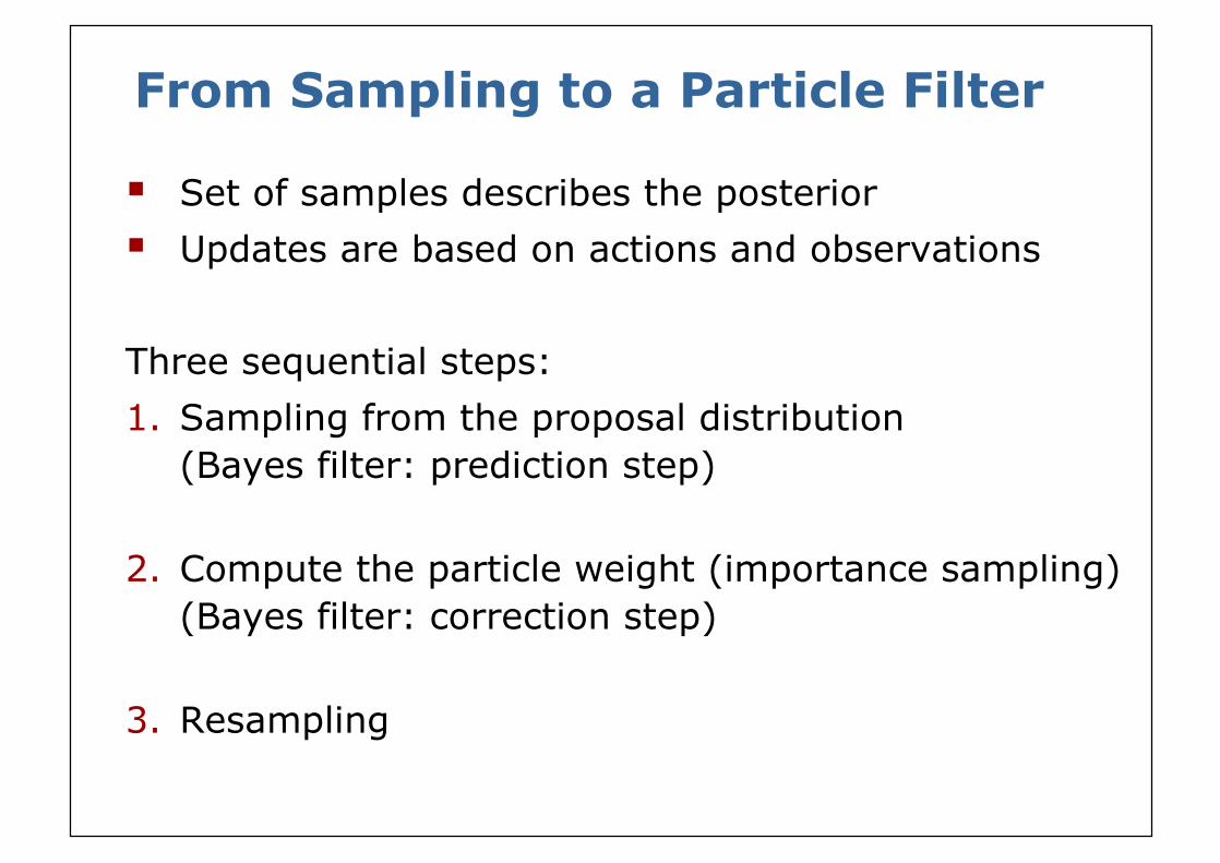
§ Set of samples describes the posterior
§ Updates are based on actions and observations
Three sequential steps:
1. Sampling from the proposal distribution (Bayes filter: prediction step)
2. Compute the particle weight (importance sampling)(Bayes filter: correction step)
3. Resampling
From Sampling to a Particle Filter

§ For each motion ∆ do:§ Sampling: Generate from each sample in
a new sample according to the motion model
§ For each observation do:
§Weight the samples with the observation likelihood
§ Resampling
Monte-Carlo Localization

Sample-based Localization (sonar)
Courtesy of Dieter Fox[video]

Grids Maps
§ Grid maps are a discretization of the
environment into free and occupied cells
§ Mapping with known robot poses is easy.

Mapping using Raw Odometry
§ Why is SLAM hard? Chicken and egg problem:
§ a map is needed to localize the robot and
§ a pose estimate is needed to build a map
Courtesy of Dirk Haehnel[video]

§ Particle filters have successfully been applied
to localization, can we use them to solve the
SLAM problem?
§ Posterior over poses x and maps m
Observations:
§ The map depends on the poses of the robot
during data acquisition
§ If the poses are known, mapping is easy
SLAM with Particle Filters
(localization) (SLAM)

Rao-Blackwellization
Factorization first introduced by Murphy in 1999
poses map observations & movements

Rao-Blackwellization
SLAM posterior
Robot path posterior
Mapping with known poses
Factorization first introduced by Murphy in 1999
poses map observations & movements

Rao-Blackwellization
This is localization, use MCL
Use the pose estimate from the MCL and apply
mapping with known poses

A Solution to the SLAM Problem
nUse a particle filter to represent potential trajectories of the robot
n Each particle carries its own map
n Each particle survives with a probability proportional to the likelihood of the observations relative to its own map
nWe have a joint posterior about the poses of the robot and the map
[Murphy, 99; Montemerlo et al., 03; Haehnel et al., 03; Eliazar and Parr, 03; Grisetti et al., 05]
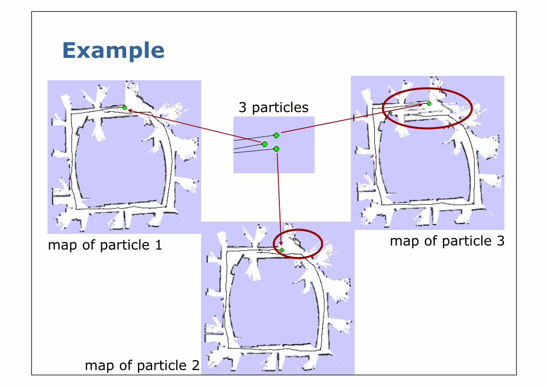
Example
map of particle 1 map of particle 3
map of particle 2
3 particles

A Graphical Model of Rao-Blackwellized Mapping
m
x
z
u
x
z
u
2
2
x
z
u
... t
t
x 1
1
0
10 t-1

Problems in Practice
§ Each map is quite big in case of grid maps§ Since each particle maintains its own map§ Therefore, one needs to keep the number
of particles small
§ Solution:Compute better proposal distributions
§ Idea:Improve the pose estimate before applying the particle filter

Pose Correction Using Scan Matching
Maximize the likelihood of the i-th pose relative to the (i-1)-th pose
robot motioncurrent measurement
map constructed so far

Motion Model for Scan Matching
Raw OdometryScan Matching
Courtesy of Dirk Haehnel

Mapping using Scan Matching
Courtesy of Dirk Haehnel
[video]

RBPF-SLAM with Improved Odometry
§ Scan-matching provides a locally consistent pose correction
§ Pre-correct short odometry sequences using scan-matching and use them as input to the Rao-Blackwellized PF
§ Fewer particles are needed, since the error in the input in smaller
[Haehnel et al., 2003]
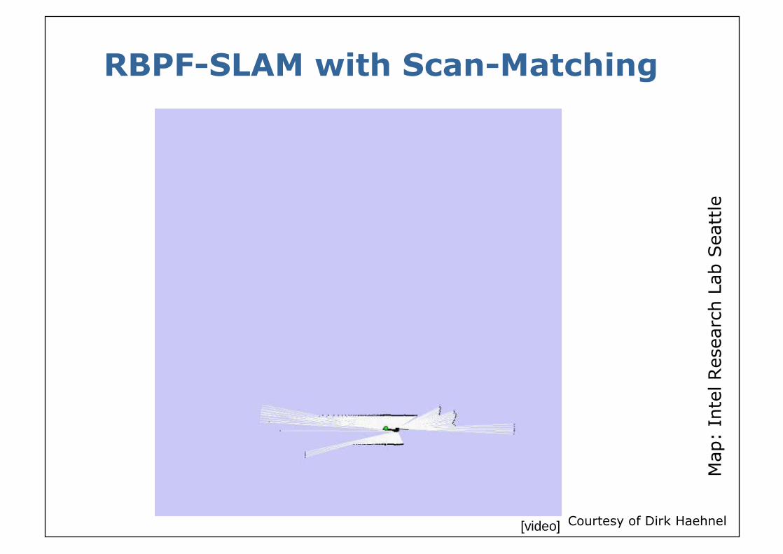
RBPF-SLAM with Scan-Matching
Map
: In
tel Res
earc
h L
ab S
eatt
le
Courtesy of Dirk Haehnel[video]

Graphical Model for Mapping with Improved Odometry
m
z
kx
1u'
0uzk-1
...1z ...
uk-1 ...k+1z
uk zu2k-1
2k-1...
x0
k
x2k
z2k
...
u'2u' n
...
xn·k
zu u(n+1)·k-1n·k
n·k+1
...(n+1)·k-1z...
n·kz
...
...

Comparison to Standard RBPF-SLAM
§ Same model for observations
§ Odometry instead of scan matching as input
§ Number of particles varying from 500 to 2.000
§ Typical result:
Courtesy of Dirk Haehnel

Conclusion (so far…)
n The presented approach is efficient
n It is easy to implement
n Scan matching is used to transform sequences of laser measurements into odometry measurements
n Provides good results for most datasets

What’s Next?
n Further reduce the number of particles
n Improved proposals will lead to more accurate maps
n Use the properties of our sensor when drawing the next generation of particles

The Optimal Proposal Distribution
For lasers is extremely peaked and dominates the product.
[Doucet, 98]
We can safely approximateby a constant:

Resulting Proposal Distribution
Approximate this equation by a Gaussian:
Sampled points around the maximum
maximum reported by a scan matcher
Gaussian approximation
Draw next generation of samples

Resulting Proposal Distribution
η is a normalizer Sampled around the scan-match maxima
Approximate this equation by a Gaussian:

Computing the Importance Weight
Sampled points around the maximum of the observation likelihood

Improved Proposal
End of a corridor:
Corridor:
Free space:

Resampling
n In case of suboptimal/bad proposal distributions resampling is necessary to achieve convergence
n Resampling is dangerous, since important samples might get lost(particle depletion problem)
t-3 t-2 t-1 t

When to Resample?
n Key question: When should we resample?
n Resampling makes only sense if the samples have significantly different weights
t-3 t-2 t-1 t

Effective Number of Particles
nEmpirical measure of how well the goal distribution is approximated by samples drawn from the proposal
n Neff describes “the variance of the particle weights”
n Neff is maximal for equal weights. In this case, the distribution is close to the proposal

Resampling with Neff
n If our approximation is close to the proposal, no resampling is needed
n We only resample when Neff drops below a given threshold (N/2)
n See [Doucet, ’98; Arulampalam, ’01]

Typical Evolution of Neff
visiting new areas closing the
first loop
second loop closure
visiting known areas

§ 15 particles
§ four times faster than real-timeP4, 2.8GHz
§ 5cm resolution during scan matching
§ 1cm resolution in final map
Intel Research Lab
[video]

Outdoor Campus Map
§ 30 particles
§ 250x250m2
§ 1.75 km (odometry)
§ 20cm resolution during scan matching
§ 30cm resolution in final map
§ 30 particles
§ 250x250m2
§ 1.088 miles (odometry)
§ 20cm resolution during scan matching
§ 30cm resolution in final map
[video]

MIT Killian Court
§ The “infinite-corridor-dataset” at MIT

MIT
Killian
Co
urt

MIT
Killian
Co
urt
Dat
aset
court
esy
of M
ike
Boss
ean
d J
ohn L
eonar
d
[video]
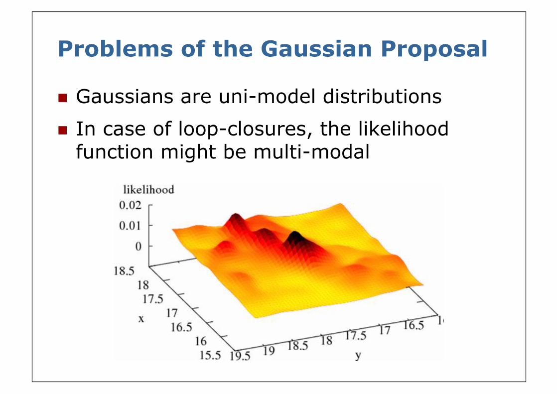
Problems of the Gaussian Proposal
n Gaussians are uni-model distributions
n In case of loop-closures, the likelihood function might be multi-modal

Is a Gaussian an Accurate Representation for the Proposal?

Problems of the Gaussian Proposal
n Multi-modal likelihood function can cause filter divergence

n Sampling from the optimal proposal:n Compute the full 3d histogramn Sample from the histogram
How to Overcome this Limitation?

How to Overcome this Limitation?
n Approximate the likelihood in a better way!
n Sample from odometry first and the use this as the start point for scan matching
odometry
mode 1 mode 2
odometry with uncertainty

Final Approach
n It work’s with nearlyzero overhead

Conclusion
n Rao-Blackwellized Particle Filters are means to represent a joint posterior about the poses of the robot and the map
n Utilizing accurate sensor observation leads to good proposals and highly efficient filters
n It is similar to scan-matching on a per-particle base with some extra noise
n The number of necessary particles andre-sampling steps can seriously be reduced
n How to deal with non-Gaussian observation likelihood functions
n Highly accurate and large scale map

More Details
n M. Montemerlo, S. Thrun, D. Koller, and B. Wegbreit. FastSLAM: Afactored solution to simultaneous localization and mapping, AAAI02(The classic FastSLAM paper with landmarks)
n M. Montemerlo, S. Thrun D. Koller, and B. Wegbreit. FastSLAM 2.0: An improved particle filtering algorithm for simultaneous localization and mapping that provably converges, IJCAI03.(FastSLAM 2.0 – improved proposal for FastSLAM)
n D. Haehnel, W. Burgard, D. Fox, and S. Thrun. An efcient FastSLAM algorithm for generating maps of large-scale cyclic environments from raw laser range measurements, IROS03(FastSLAM on grid-maps using scan-matched input)
n A. Eliazar and R. Parr. DP-SLAM: Fast, robust simultainouslocalization and mapping without predetermined landmarks, IJCAI03 (A representation to handle big particle sets)

More Details (Own Work)
n Giorgio Grisetti, Cyrill Stachniss, and Wolfram Burgard. Improved Techniques for Grid Mapping with Rao-Blackwellized Particle Filters, Transactions on Robotics, Volume 23, pages 34-46, 2007(Informed proposal using laser observation, adaptive resampling)
n G. Grisetti, C. Stachniss, and W. Burgard. Improving grid-based slam with rao-blackwellized particle filters by adaptive proposals and selective resampling, ICRA’05(Informed proposal using laser observation, adaptive resampling)
n Cyrill Stachniss, Grisetti Giorgio, Wolfram Burgard, and Nicholas Roy. Analyzing Gaussian Proposal Distributions for Mapping with Rao-Blackwellized Particle Filters, IROS07(Gaussian assumption for computing the improved proposal)

From Theory to Practice
n Implementation available a open source project “GMapping” on
www.OpenSLAM.org
n Written in C++
n Can be used as a black box library
Now: 1h Practical Course on GMapping