Embed Size (px)
Citation preview

RANDOMIZED PRIMITIVES FOR LINEAR ALGEBRA AND APPLICATIONS
by
Anastasios Zouzias
A thesis submitted in conformity with the requirementsfor the degree of Doctor of Philosophy
Graduate Department of Computer ScienceUniversity of Toronto
c© Copyright 2013 by Anastasios Zouzias
Abstract
RANDOMIZED PRIMITIVES FOR LINEAR ALGEBRA AND APPLICATIONS
Anastasios Zouzias
Doctor of Philosophy
Graduate Department of Computer Science
University of Toronto
2013
The present thesis focuses on the design and analysis of randomized algorithms for accelerating several
linear algebraic tasks. In particular, we develop simple, efficient, randomized algorithms for a plethora
of fundamental linear algebraic tasks and we also demonstrate their usefulness and applicability to
matrix computations and graph theoretic problems. The thesis can be divided into three parts. The
first part concentrates on the development of randomized linear algebraic primitives, the second part
demonstrates the application of such primitives to matrix computations, and the last part discusses the
application of such primitives to graph problems.
First, we present randomized approximation algorithms for the problems of matrix multiplication,
orthogonal projection, vector orthonormalization and principal angles computation (a.k.a. canonical
correlation analysis).
Second, utilizing the tools developed in the first part, we present randomized and provable accurate
approximation algorithms for the problems of linear regression and element-wise matrix sparsification.
Moreover, we present an efficient deterministic algorithm for selecting a small subset of vectors that are
in isotropic position.
Finally, we exploit well-known interactions between linear algebra and spectral graph theory to
develop and analyze graph algorithms. In particular, we present a near-optimal time deterministic
construction of expanding Cayley graphs, an efficient deterministic algorithm for graph sparsification
and a randomized distributed Laplacian solver that operates under the gossip model of computation.
ii

Dedication
Dedicated to the memory of Avner Magen
iii
Acknowledgements
The completion of this manuscript was made possible through the invaluable contributions of a number
of people. First, I would like to express my gratitude to my supervisors Mark Braverman and Avner
Magen. They both provided me with a deep perspective of theoretical computer science and guidance
on many technical aspects of this thesis. Their inspiration has been truly invaluable to me. Moreover, I
would like to thank Allan Borodin, Steve Cook, Ken Jackson, Mike Molloy and Toni Pitassi for agreeing
to serve as members of my final examination committee. Moreover, I would like to sincerely thank Joel
A. Tropp for his careful assessment of my work and for providing useful suggestions for improvements.
During my time in graduate school, I had the great pleasure to collaborate with many researchers.
I would like to thank all my co-authors: Haim Avron, Christos Boutsidis, Petros Drineas, Jeff Ed-
monds, Nick Freris, Piotr Indyk, Pascal Koiran, Avner Magen, Mike Mahoney, Tassos Sidiropoulos,
Sivan Toledo and Michail Vlachos. I truly enjoyed collaborating with them and I have learned a lot
from each one of them.
The department of computer science at the university of Toronto (UofT) is a great academic environ-
ment with many great scholars. In particular, I would like to thank all the members of the theory group.
I have also learned a lot from fellow graduate students and postdocs especially Aki, Arkadev, Bren-
dan, Costis, Dai, Eden, George, Jeremy, Joel, Kaveh, Lila, Natan, Per, Periklis, Siavosh, Tassos, Wesley,
Yevgeniy, Yu and Yuval.
Many thanks go to IBM Research Zurich for hosting me as a research intern during the summer and
fall of 2011. The initial discussions about the randomized gossip algorithms of Chapter 4 were initiated
there. In addition, I would like to thank the department of computer science at Princeton University for
hosting me as a visiting student during the winter of 2012 (especially Mark for setting up everything).
I would like to thank all Greek graduate students at UofT (a.k.a. Greek mafia or “grspamites”) for
all the moments of joy and fun that we shared together. Last but not least, I would like to thank Maria
for her support, encouragement, and for making my journey through graduate school, pleasant and
full of beautiful moments.
Finally, my heartfelt thanks go out to my family and friends in Greece for their constant support
and encouragement.
iv

Contents
1 Introduction 1
1.1 Organization of the Thesis . . . . . . . . . . . . . . . . . . . . . . . . . . . . . . . . . . . . . 2
1.2 Preliminaries . . . . . . . . . . . . . . . . . . . . . . . . . . . . . . . . . . . . . . . . . . . . . 5
2 Randomized Approximate Linear Algebraic Primitives 18
2.1 Approximate Matrix Multiplication . . . . . . . . . . . . . . . . . . . . . . . . . . . . . . . 18
2.2 Approximate Orthogonal Projection . . . . . . . . . . . . . . . . . . . . . . . . . . . . . . . 27
2.3 Approximate Orthonormalization . . . . . . . . . . . . . . . . . . . . . . . . . . . . . . . . 29
2.4 Approximate Principal Angles . . . . . . . . . . . . . . . . . . . . . . . . . . . . . . . . . . 33
3 Matrix Algorithms 44
3.1 Randomized Approximate Least Squares . . . . . . . . . . . . . . . . . . . . . . . . . . . . 44
3.2 Fast Isotropic Sparsification . . . . . . . . . . . . . . . . . . . . . . . . . . . . . . . . . . . . 60
3.3 Element-wise Matrix Sparsification . . . . . . . . . . . . . . . . . . . . . . . . . . . . . . . . 65
4 Graph Algorithms 77
4.1 Alon-Roichman Expanding Cayley Graphs . . . . . . . . . . . . . . . . . . . . . . . . . . . 77
4.2 Deterministic Graph Sparsification . . . . . . . . . . . . . . . . . . . . . . . . . . . . . . . . 80
4.3 Randomized Gossip Algorithms for Solving Laplacian Systems . . . . . . . . . . . . . . . 82
5 Conclusions 93
Bibliography 97
v

Chapter 1Introduction
Randomness has served as an important resource and indispensable idea in the theory of computa-
tion. There is a plethora of successful paradigms of the use of randomness in theoretical computer
science including complexity theory (interactive proofs, PCP), distributed computation, and random-
ized approximation algorithms in combinatorial optimization (randomized rounding), computational
geometry (coresets) and machine learning theory (VC-dimension), to name a few. Randomness has
also been the driving force in discrete mathematics towards a better understanding of combinatorial
structures via the probabilistic method.
The present thesis focuses on the following fundamental question:
How can we utilize randomness to accelerate linear algebraic computations?
The design and analysis of deterministic “exact” algorithms for linear algebraic tasks including
multiplying matrices, solving a system of linear equations, computing the rank, the singular values or
any other interesting quantities associated with matrices has a very rich literature both in the pure and
the applied mathematics literature [Dem97, GL96].
On the other hand, the first appearance of a randomized algorithm for approximating matrix com-
putations via dimensionality reduction appeared in the papers of Papadimitriou et al. [PRTV98] and
Frieze et al. [FKV98]. The authors of [PRTV98], motivated by an application to term-document indexing
(latent semantic indexing), proposed a randomized algorithm for efficient low rank matrix approxima-
tion using random projections. The paper of [FKV98] analyzed a randomized dimensionality reduction
approach utilizing non-uniform row/column sampling for the low rank matrix approximation prob-
lem. In the sequel, the idea of utilizing randomness to approximate matrices inspired researchers to de-
sign and analyze randomized algorithms for approximating matrix multiplication [DKM06a], low rank
1

CHAPTER 1. INTRODUCTION 2
matrix approximation [FKV04, DKM06b, LWM+07, HMT11] and matrix decomposition [DKM06c] to
name a few. Most of this work was motivated by the need of processing very large data-sets which
are usually modeled by a matrix representation. In particular, a large body of work on the the design
of randomized algorithms for large matrix problems has been recently developed. The current state
of the rapidly growing literature in this research area has been partially summarized in the following
surveys [Mah11, KV09, HMT11].
The scope of this thesis is to contribute to the aforementioned line of research by designing and
analyzing simple, efficient, randomized approximation algorithms for several fundamental linear alge-
braic tasks and, in addition, demonstrate their usefulness and applicability to matrix computations and
graph theoretic problems.
1.1 Organization of the Thesis
Below, we outline the structure of this thesis and highlight the contributions of the individual chapters.
The thesis can be divided into three parts. The first part, consisting mainly of Chapter 2, concentrates on
the design and analysis of several randomized linear algebraic primitives. The second part (Chapter 3)
demonstrates the application of such linear algebraic tools to several matrix computations. Finally, the
third part (Chapter 4) discusses the application of such primitives to graph theoretic problems.
Chapter 2: Randomized Approximate Linear Algebraic Primitives
Chapter 2 discusses randomized linear algebraic primitives such as approximate matrix multiplication,
approximate orthogonal projection, approximate vector orthonormalization and approximate compu-
tation of a particular notion of distance between two linear subspaces. Below we briefly outline the
main contributions of this chapter.
The research of [FKV04] focuses on using non-uniform row sampling to speed-up the running time
of several matrix computations. The subsequent developments of [DKM06a, DKM06b, DKM06c] also
study the performance of Monte-Carlo algorithms on primitive matrix algorithms including the matrix
multiplication problem with respect to the Frobenius norm, see also [RV07]. Sarlos [Sar06] extended
(and improved) this line of research using random projections. Here, following the above line of re-
search, we improve the analysis of the above randomized algorithms for approximating matrix multi-
plication with respect to the operator norm.
In addition, a randomized iterative algorithm for approximately computing orthogonal projections

CHAPTER 1. INTRODUCTION 3
is presented. That is, given any vector and linear subspace represented as the column span of a matrix
A, the proposed algorithm converges exponentially to the orthogonal projection of the given vector
onto the column span of A. The convergence rate of the algorithm depends, roughly speaking, on the
condition number of A.
Based on the aforementioned approximate orthogonal projection algorithm, we present a random-
ized iterative, amenable to parallel implementation, algorithm for orthonormalizing a set of high di-
mensional vectors. The algorithm might be effective compared to the classical Gram Schmidt orthonor-
malization for the case of sparse and sufficiently well-conditioned set of vectors.
Finally, an efficient randomized algorithm for approximating the principal angles and principal
vectors between two subspaces is presented. To the best of our knowledge, the proposed algorithm is
the first provable accurate approximation algorithm that is more efficient than the state-of-the-art exact
algorithms [GZ95] for the case of very high-dimensional subspaces. This chapter is based on joint work
with Freris [ZF12] and on joint work with Avron, Boutsidis and Toledo [ABTZ12]
Chapter 3: Matrix Algorithms
In Chapter 3, we present randomized and provable accurate approximate algorithms for the problems
of linear regression and element-wise matrix sparsification. Moreover, we analyze an efficient deter-
ministic algorithm for selecting a small subset of vectors that are in isotropic position. Below, we briefly
outline the main contributions of this chapter.
We present a randomized iterative algorithm that, given any system of linear equations, exponen-
tially converges in expectation to the minimum Euclidean norm least squares solution. The expected
number of arithmetic operations required to obtain an estimate of given accuracy is proportional to
the square condition number of the system multiplied by the number of non-zeros entries of the input
matrix. The proposed algorithm which we call randomized extended Kaczmarz is an extension of the ran-
domized Kaczmarz method that was analyzed by Strohmer and Vershynin and resolves a question left
open in [SV06, SV09].
Given a set of vectors in isotropic position, we present an efficient deterministic algorithm for select-
ing a subset of thes vectors that are approximately close to isotropic position. The proposed algorithm
builds on important and strong results from numerical linear algebra including the Fast Multipole
Method [CGR88] (FMM) and eigenvalue solvers of matrices after rank-one updates [GE94].
Element-wise matrix sparsification was pioneered by Achlioptas and McSherry [AM01, AM07].
Achlioptas and McSherry described sampling-based algorithms that select a small number of entries

CHAPTER 1. INTRODUCTION 4
from an input matrix A to construct a sparse sketch A, which is close to A in the operator norm.
We present a simple matrix sparsification algorithm that achieves the best known upper bounds for
element-wise matrix sparsification and its analysis is based on matrix concentration inequalities. More-
over, using the matrix hyperbolic cosine algorithm (Section 1.2.6), we present the first deterministic
algorithm and strong sparsification bounds for symmetric matrices that have an approximate diago-
nally dominant property. This chapter is based on joint work with Magen [MZ11], on joint work with
Drineas [DZ11] and on joint work with Freris [ZF12].
Chapter 4: Graph Algorithms
It is well-known that linear algebra serves as an extremely useful tool for analyzing and understand-
ing several properties of graphs, most notably graph expansion. In this chapter, we exploit such con-
nections to design and analyze graph algorithms such as near-optimal deterministic constructions of
expanding Cayley graphs, efficient deterministic algorithms for graph sparsification and Laplacian
solvers under the gossip (a.k.a. epidemic) model of distributed computation.
First, the Alon-Roichman theorem asserts that Cayley graphs obtained by choosing a logarithmic
number of group elements independently and uniformly at random are expanders [AR94]. Wigderson
and Xiao’s derandomization of the matrix Chernoff bound implies a deterministic O(n4 log n) time al-
gorithm for constructing Alon-Roichman graphs [WX08]. Independently, Arora and Kale generalized
the multiplicative weights update (MWU) method to the matrix-valued setting and, among other in-
teresting implications, they improved the running time to O(n3 polylog (n)) [Kal07]. Here we further
improve the running time to O(n2 log3 n) utilizing the matrix hyperbolic cosine algorithm and exploit-
ing the group structure of the problem.
Second, the spectral graph sparsification problem poses the question whether any dense graph can
be approximated by a sparse graph while preserving all eigenvalues of the difference of their Laplacian
matrices to an arbitrarily small relative error [Spi10]; the resulting graphs are usually called spectral spar-
sifiers. An efficient randomized algorithm to construct an (1 + ε)-spectral sparsifier with O(n log n/ε2)
edges was given in [SS08]. Furthermore, an (1 + ε)-spectral sparsifier with O(n/ε2) edges can be com-
puted in O(mn3/ε2) deterministic time [BSS09]. Here we present an efficient deterministic algorithm
for spectrally sparsifying dense graphs. The main contribution here is the following: given a weighted
dense graph H = (V, E) on n vertices with positive weights and 0 < ε < 1, there is a deterministic algo-
rithm that returns an (1 + ε)-spectral sparsifier with O(n/ε2) edges in O(n4 log n/ε2 maxlog2 n, 1/ε2)
time.

CHAPTER 1. INTRODUCTION 5
Third, we present a randomized distributed algorithm for solving Laplacian linear systems with
exponential convergence in expectation under the gossip model of computation. Gossip algorithms
for distributed computation are based on a gossip or rumor-spreading type of asynchronous message
exchange protocol. The analysis of the proposed algorithm relies on the advances in randomized itera-
tive least squares solvers including the randomized extended Kaczmarz method discussed in Chapter 3.
This chapter is based on joint work with Freris [FZ12] and on the work of [Zou12].
1.2 Preliminaries
We now introduce the mathematical notation that will be used throughout the thesis and we also
present several basic results from linear algebra and probability theory. In addition, we state known
facts about uniform sampling rows from matrices with orthonormal columns and we present the ma-
trix Bernstein inequality and Minsker’s version of the matrix Bernstein inequality [Min11]. Finally, we
present a matrix generalization of Spencer’s hyperbolic cosine algorithm [Spe77]
Basic Notation For an integer m, let [m] := 1, . . . , m. We denote by R, Z and N the reals, integers and
natural numbers, respectively. For any positive number x, the base-2 logarithm and natural logarithm
of x is denoted by log(x) and ln(x), respectively. Occasionally, we might prefer to hide log log(·) factors
under the big-Oh notation, we make this explicit by using O(·). All matrices contain real entries. We use
capital letters A, B, . . . to denote matrices and bold lower-case letters x,y, . . . to denote column vectors.
We denote by 0, the all-zeroes matrix, J for the all-ones matrix and I for the identity matrix and by
e1, e2, . . . , en the standard basis vectors of Rn. Occasionally, we explicitly specify the dimensions of
these matrices by adding a subscript, e.g., In is the n × n identity matrix. Sn×n denotes the set of
symmetric matrices of size n. We denote the rows and columns of any m× n matrix A by A(1), . . . , A(m)
and A(1), . . . , A(n), respectively. R(A) denotes the range (or column span) of A, i.e., R(A) := Ax | x ∈
Rn and R(A)⊥ denotes the orthogonal complement of R(A). Let x ∈ R
n, we denote by diag (x) the
diagonal matrix containing x1, x2, . . . , xn. For a square matrix M, we also write diag (M) to denote the
diagonal matrix that contains the diagonal entries of M. Let x ∈ Rn and y ∈ R
n viewed as row or
column vectors, then x⊗ y is the n× n matrix such that (x⊗ y)i,j = xiyj . We denote the inner product
between two vectors x and y of the same dimensions by 〈x, y〉 :=∑
i xiyi. We denote by [A; B] the
matrix obtained by concatenating the columns of B next to the columns of A. Moreover, we denote by
nnz (·) the number of non-zero entries of its argument matrix.

CHAPTER 1. INTRODUCTION 6
1.2.1 Linear Algebra
The following discussion reviews several definitions and facts from linear algebra; for more details,
see [Bha96, GL96, HJ90]. Let A be an m×n matrix of rank r. We denote ‖A‖2 = max‖Ax‖2 | ‖x‖2 = 1,
‖A‖∞ = maxi∈[m]
∑j∈[n] |aij | and by ‖A‖F =
√∑i,j a2
ij the Frobenius norm of A. Also rank (A) and
sr (A) := ‖A‖2F / ‖A‖22 is the rank and stable rank of A. Observe that sr (A) ≤ rank (A). The trace of a
square matrix B, i.e., the sum of its diagonal elements, is denoted as tr (B). A matrix P of size n is called
projector if it is idempotent, i.e., P2 = P.
A symmetric matrix A is positive semi-definite (PSD), denoted by 0 A, if x⊤Ax ≥ 0 for every
vector x. For two symmetric matrices X, Y, we say that Y X if and only if Y − X is a positive semi-
definite (PSD) matrix. Moreover, a symmetric matrix A of size n is called diagonally dominant if |Aii| ≥
∑j 6=i |Aij | for every i ∈ [n]. Given any matrix A, its dilation is defined as D (A) =
0 A
A⊤ 0
. It is easy
to verify that λmax(D (A)) = ‖A‖2.
Let A = UΣV⊤ be the truncated singular value decomposition (SVD) of A where U ∈ Rm×r with
U⊤U = Ir, Σ is the diagonal matrix of size r containing the non-zero singular values σ1(A), σ2(A), . . . , σr(A)
of A in non-increasing order, and V ∈ Rn×r with V⊤V = Ir. The singular value decomposition can be
computed using O(mn min(m, n)) arithmetic operations. Whenever the matrix A is clear from the con-
text, we will refer to σ1(A) and σrank(A)(A) as σmax and σmin, respectively. The Moore-Pensore pseudo-
inverse of A is denoted by A† := VΣ−1U⊤. Recall that∥∥A†∥∥
2= 1/σmin. For any non-zero real matrix A,
we define
κ2F (A) := ‖A‖2F
∥∥A†∥∥2
2. (1.1)
Related to this is the scaled square condition number introduced by Demmel in [Dem88], see also [SV09].
It is easy to check that the above parameter κ2F (A) is related with the condition number of A, cond (A) :=
σmax/σmin, via the inequalities: cond (A)2 ≤ κ2
F(A) ≤ rank (A) · cond
(A2)2
. We denote by nnz (·) the num-
ber of non-zero entries of its argument matrix. We define the average row sparsity and average column
sparsity of A by Ravg and Cavg, respectively, as follows:
Ravg :=
m∑
i=1
qi nnz
(A
(i))
and Cavg :=
n∑
j=1
pj nnz(A(j)
)
where pj :=∥∥A(j)
∥∥2
2/ ‖A‖2F for every i ∈ [n] and qi :=
∥∥A(i)∥∥2
2/ ‖A‖2F for every i ∈ [m]. The following
fact will be used in Chapter 3.
Fact 1.1. Let A be any non-zero real m× n matrix and b ∈ Rm. Denote by xLS := A†b. Then xLS = A†bR(A).

CHAPTER 1. INTRODUCTION 7
Finally, we frequently use the inequality 1− t ≤ exp(−t) for every t ≤ 1.
Functions of Matrices. Here we review some basic facts about matrix functions including the ma-
trix exponential and the matrix hyperbolic cosine function, for more details see [Hig08]. The matrix
exponential of a symmetric matrix A is defined as exp [A] = I +∑∞
k=1A
k
k! . Let A = QΛQ⊤ be the eigen-
decomposition of A. It is easy to see that exp [A] = Q exp [Λ] Q⊤. For any square matrices A and B of the
same size that commute, i.e., AB = BA, we have that exp [A + B] = exp [A] exp [B]. In general, when A
and B do not commute, the following estimate is known for symmetric matrices.
Lemma 1.2. [Gol65, Tho65] For any symmetric matrices A and B, tr (exp [A + B]) ≤ tr (exp [A] exp [B]).
The following fact about matrix exponential for rank one matrices will be also useful.
Lemma 1.3. Let x be a non-zero vector in Rn. Then exp [x⊗ x] = In + e‖x‖2
2−1‖x‖2
2
x⊗x. Similarly, exp [−x⊗ x] =
In − 1−e−‖x‖22
‖x‖22
x⊗ x.
Proof. The proof is immediate by the definition of the matrix exponential. Notice that (x ⊗ x)k =
‖x‖2(k−1)2 x⊗ x for k ≥ 1, hence
exp [x⊗ x] = I +
∞∑
k=1
(x⊗ x)k
k!= I +
∞∑
k=1
‖x‖2(k−1)2 x⊗ x
k!= I +
e‖x‖22 − 1
‖x‖22x⊗ x.
Similar considerations give that exp [−x⊗ x] = I− 1−e−‖x‖22
‖x‖22
x⊗ x.
Let us define the matrix hyperbolic cosine function of a symmetric matrix A as cosh [A] := (exp [A] +
exp [−A])/2. Next, we state a few properties of the matrix hyperbolic cosine.
Lemma 1.4. Let A be a symmetric matrix of size n. Then tr (exp [D (A)]) = 2 tr (cosh [A]).
Proof. Set B := D (A) =
0 A
A⊤ 0
. Notice that for any integer k ≥ 1, B2k =
A2k 0
0 A2k
and B2k+1 =
0 A2k+1
A2k+1 0
. Since the odd powers of B are trace-less, it follows that
tr (exp [B]) = tr
(I2n +
∞∑
k=1
B2k
(2k)!+
∞∑
k=0
B2k+1
(2k + 1)!
)= tr
(I2n +
∞∑
k=1
B2k
(2k)!
)
= 2 tr
(In +
∞∑
k=1
A2k
(2k)!
)= tr (exp [A] + exp [−A]) = 2 tr (cosh [A]) .

CHAPTER 1. INTRODUCTION 8
Lemma 1.5. Let A be a symmetric matrix and P be a projector matrix that commutes with A, i.e., PA = AP.
Then cosh [PA] = P cosh [A] + I− P.
Proof. By the definition of cosh [·], it suffices to show that exp [PA] = P exp [A] + I− P,
exp [PA] = I +
∞∑
k=1
(PA)k
k!= I + P
∞∑
k=1
Ak
k!= P exp [A] + I− P.
Lemma 1.6. For any positive semi-definite symmetric matrix A of size n and any two symmetric matrices B, C
of size n, B C implies tr (AB) ≤ tr (AC).
Proof. Conjugating by A1/2 the PSD inequality B C (Lemma 1.10), it follows that A1/2BA1/2
A1/2CA1/2. Taking the trace operator over both sides implies that tr(A1/2BA1/2
)≤ tr
(A1/2CA1/2
).
To conclude use the cyclic property of the trace on both sides, i.e., tr(A1/2BA1/2
)= tr
(A1/2A1/2B
)=
tr (AB).
Matrix Perturbation. The next discussion reviews a few results from matrix perturbation theory; for
more details, see [SS90, GL96, Bha96]. The next lemma states that if a symmetric positive semi-definite
matrix C approximates the Rayleigh quotient of a symmetric positive semi-definite matrix C, then the
eigenvalues of C also approximate the eigenvalues of C.
Lemma 1.7. Let 0 < ε < 1. Assume C, C are n × n symmetric positive semi-definite matrices, such that the
following inequality holds (1 − ε)x⊤Cx ≤ x⊤Cx ≤ (1 + ε)x⊤Cx for every x ∈ Rn. Then, for i = 1, . . . , n the
eigenvalues of C and C are the same up-to an error factor ε, i.e.,
(1− ε)λi(C) ≤ λi(C) ≤ (1 + ε)λi(C).
Proof. The proof is an immediate consequence of the Courant-Fischer’s characterization of the eigenval-
ues. First notice that by hypothesis, C and C have the same null space. Hence we can assume without
loss of generality, that λi(C), λi(C) > 0 for all i = 1, . . . , n. Let λi(C) and λi(C) be the eigenvalues (in
non-decreasing order) of C and C, respectively. The Courant-Fischer min-max theorem [GL96, p. 394]
expresses the eigenvalues as
λi(C) = minSi
maxx∈Si
x⊤Cx
x⊤x, (1.2)
where the minimum is over all i-dimensional subspaces Si. Let the subspaces Si0 and Si
1 where the

CHAPTER 1. INTRODUCTION 9
minimum is achieved for the eigenvalues of C and C, respectively. Then, it follows that
λi(C) = minSi
maxx∈Si
x⊤Cx
x⊤x≤ max
x∈Si0
x⊤Cx
x⊤Cx
x⊤Cx
x⊤x≤ (1 + ε)λi(C).
and similarly,
λi(C) = minSi
maxx∈Si
x⊤Cx
x⊤x≤ max
x∈Si1
x⊤Cx
x⊤Cx
x⊤Cx
x⊤x≤ λi(C)
1− ε.
Therefore, it follows that for i = 1, . . . , n: (1− ε)λi(C) ≤ λi(C) ≤ (1 + ε)λi(C).
We now state two known matrix perturbation results and a simple but useful property of the psd
ordering.
Lemma 1.8 (Theorem 3.3 in [EI95]). Let Ψ ∈ Rp×q and Φ = DLΨDR with DL ∈ R
p×p and DR ∈ Rq×q
being non-singular matrices. Let γ = max∥∥DLD⊤
L − Ip
∥∥2,∥∥D⊤
RDR − Iq
∥∥2. Then, for all i = 1, . . . , rank (Ψ):
|σi (Φ)− σi (Ψ) | ≤ γ · σi (Ψ) .
Lemma 1.9 (Weyl’s inequality for singular values; Corollary 7.3.8 in [HJ90]). Let Φ, Ψ ∈ Rm×n. Then, for
all i = 1, . . . , min(m, n) : |σi (Φ)− σi (Ψ) | ≤ ‖Φ−Ψ‖2.
Lemma 1.10 (Conjugating the PSD ordering; Observation 7.7.2 in [HJ90]). Let Φ, Ψ ∈ Rn×n are symmetric
matrices with Φ Ψ. Then, for every n×m matrix Z : Z⊤ΦZ Z⊤ΨZ.
1.2.2 Probabilistic Tools
We abbreviate the terms “independently and identically distributed” and “almost surely” with i.i.d.
and a.s., respectively.
The first tool is the so-called subspace Johnson-Lindenstrauss lemma. Such a result was obtained
in [Sar06] (see also [Cla08, Theorem 1.3]) although it appears implicitly in results extending the origi-
nal Johnson Lindenstrauss lemma [JL84] (see [Mag07]). The techniques for proving such a result with
possible worse bound are not new and can be traced back even to Milman’s proof of Dvoretsky theo-
rem [Mil71].
Lemma 1.11. (Subspace JL lemma [Sar06]) LetW ⊆ Rd be a linear subspace of dimension k and ε ∈ (0, 1/3).
Let R be a t× d random sign matrix rescaled by 1/√
t, namely Rij = ±1/√
t with equal probability. Then
P
((1− ε) ‖w‖22 ≤ ‖Rw‖22 ≤ (1 + ε) ‖w‖22 , ∀ w ∈ W
)≥ 1− ck
2 · exp(−c1ε2t), (1.3)
where c1 = 116·36 , c2 = 18.

CHAPTER 1. INTRODUCTION 10
Proof. The statement in our lemma has been proved in Corollary 11 of [Sar06], see also [Cla08, Theo-
rem 1.3] for a restatement. More precisely, repeat the proof of Corollary 11 of [Sar06] paying attention
to the constants. That is, set C = W⊤R⊤RW− Ik where the column span of W equals toW and ε0 = 1/2
in Lemma 10 of [Sar06]. Then, apply the JL transform [Ach03] with (rescaled) accuracy ε/4 on each
vector of the set T ′ := W⊤x | x ∈ T where T is from Lemma 10 of [Sar06], hence |T ′| ≤ ek ln(18). So,
P((∀i = 1, . . . , k : 1− ε ≤ σi(W
⊤R⊤RW) ≤ 1 + ε))≥ 1− ek ln(18)e−ε2r/(36·16). (1.4)
Therefore, whenever the event of Ineq. (1.4) holds, it implies that ‖C‖2 =∥∥W⊤R⊤RW − Ik
∥∥2≤ ε, which
is equivalent to the statement of Ineq. (1.3).
Next we present a standard lemma that bounds the spectral norm of any matrix A when it’s mul-
tiplied by a random sign matrix that is rescaled by 1/√
t presented to us by Mark Rudelson (personal
communication, 2010). If random Gaussian matrices are used in the following lemma, then it is a di-
rect consequence of Gaussian measure concentration for Lipschitz functions. The use of random sign
matrices makes the argument a bit more involved, but such arguments are standard in the literature.
Lemma 1.12. Let A be an m × n real matrix and fix t ≥ 1. Let R be a t × n random sign matrix rescaled by
1/√
t. For every τ > 0
P
(∥∥AR⊤∥∥2≥ 2 ‖A‖F /
√t + 2 ‖A‖2 + ‖A‖2 τ/
√t)≤ e−τ2/8. (1.5)
Proof. Let G be a t× n matrix whose entries are independent Gaussian random variables. Then by the
Gordon-Chevet inequality1
E∥∥AG⊤∥∥
2≤ ‖It‖2 ‖A‖F + ‖It‖F ‖A‖2 = ‖A‖F + ‖A‖2
√t.
Let ⊙ denote the entrywise product2 (also known as Hadamard product) between two matrices of
the same size. Write G as E⊙ |G|where Eij = sign (Gij) and the (i, j) entry of |G| equals |Gij |. Note that
E and |G| are independent and E is a random sign matrix. It follows that
E[E⊙ |G| | E] =
√2
πE
since E |g| =√
2/π for a Gaussian random variable g. Multiply the above from the right with A⊤ and
1For example, set S = It,T = A in [HMT11, Proposition 10.1, p. 54].2For any two matrices B and C of the same size (B ⊙ C)ij = BijCij

CHAPTER 1. INTRODUCTION 11
take norms on both sides∥∥E[(E⊙ |G|)A⊤ | E
]∥∥2
=
∥∥∥∥∥
√2
πEA⊤
∥∥∥∥∥2
.
By Jensen’s inequality, it follows that∥∥∥√
2π EA⊤
∥∥∥2≤ E
[∥∥(E⊙ |G|)A⊤∥∥2| E]. Taking expectation with
respect to E, it follows that √2
πE∥∥EA⊤∥∥
2≤ E
∥∥GA⊤∥∥2.
Since E is a random sign matrix, it follows that
E∥∥AR
⊤∥∥2≤√
π
2tE∥∥GA
⊤∥∥2≤ 2(‖A‖F /
√t + ‖A‖2).
Define the function f : [−1, 1]t×n → R by f(S) =∥∥∥ 1√
tAS⊤
∥∥∥2. The calculation above shows that E f(S) ≤
2(‖A‖F /√
t+‖A‖2) where the expectation is over a uniformly at random element of ±1t×n. We bound
the Lipschitz constant of f . Let S1, S2 ∈ [−1, 1]t×n,
|f(S1)− f(S2)| ≤∥∥∥∥
1√tA(S⊤
1 − S⊤2 )
∥∥∥∥2
≤ 1√t‖A‖2 ‖S1 − S2‖F
where we used the triangle inequality and standard properties of matrix norms.
Since f is convex and (‖A‖2 /√
t)-Lipschitz as a function of the entries of S, Talagrand’s measure
concentration inequality for product measures [Led96, Equation 1.8] or [Led01, Theorem 5.9, p. 100]
yields that for every τ > 0
P
(∥∥AR⊤∥∥2≥ E
∥∥AR⊤∥∥2+‖A‖2 τ√
t
)≤ exp(−τ2/8).
It follows that for every τ > 0
P
(∥∥AR⊤∥∥2≥ 2(‖A‖F /
√t + ‖A‖2) + ‖A‖2 τ/
√t)≤ exp(−τ2/8).
1.2.3 Matrix Coherence and Sampling from an Orthonormal Matrix
Given a matrix A with m rows, the coherence of A is defined as µ(A) = maxi∈[m]
∥∥e⊤i UA
∥∥2, where ei is the
i-th standard basis (column) vector of Rm and UA is the set of the left singular vectors of the truncated
SVD of A. Coherence is an important quantity in the analysis of randomized matrix algorithms. Note

CHAPTER 1. INTRODUCTION 12
that the coherence of A is a property of the column space of A, and does not depend on the actual choice
of A. Therefore, if R(A) = R(B) then µ(A) = µ(B). Furthermore, it is easy to verify that ifR(A) ⊆ R(B)
then µ(A) ≤ µ(B). Finally, we mention that for every matrix A with m rows: rank (A) /m ≤ µ(A) ≤ 1.
In this thesis, we quite often focus on tall-and-thin matrices, i.e. matrices with (much) more rows
than columns. The following lemma formalizes that coherence affects the amount of rows needed to
be uniformly sampled from a matrix with orthonormal columns so that the resulting sampled matrix
remains close to orthonormal (i.e., its singular values are close to one). We need to setup the following
notation before stating the next lemma. Given a subset of indices T ⊆ [m], the corresponding sampling
matrix S is the |T | ×m matrix obtained by discarding from Im the rows whose index is not in T . Note
that SA is the matrix obtained by keeping only the rows in A whose index appears in T .
Lemma 1.13 (Sampling from Orthonormal Matrix, Corollary to Lemma 3.4 in [Tro11a]). Let Q ∈ Rm×d
have orthonormal columns. Let 0 < ε < 1 and 0 < δ < 1. Let r be an integer such that
6ε−2mµ(Q) log(3d/δ) ≤ r ≤ m .
Let T be a random subset of [m] of cardinality r, drawn from a uniform distribution over such subsets, and let S
be the |T | ×m sampling matrix corresponding to T rescaled by√
m/r. Then, with probability of at least 1 − δ,
for i ∈ [d]:√
1− ε ≤ σi(SQ) ≤√
1 + ε.
Proof. Apply Lemma 3.4 in [Tro11a] with the following choice of parameters: ℓ = αM log(k/δ), α =
6/ε2, and δtropp = η = ε. Here, ℓ, α, M , k, η are the parameters of Lemma 3.4 in [Tro11a]; also δtropp
plays the role of δ, an error parameter, of Lemma 3.4 in [Tro11a]. ε and δ are from our Lemma.
In the above lemma, T is obtained by sampling coordinates from [m] without replacement. Similar
results can be shown for sampling with replacement, or using Bernoulli variables [IW12].
1.2.4 Randomized Walsh-Hadamard Transform
Matrices with high coherence pose a problem for algorithms based on uniform row sampling. One way
to circumvent this problem is to use a coherence-reducing transformation. One popular coherence-
reducing transformation is the Randomized Walsh-Hadamard Transform (RHT) matrix introduced
in the paper of Ailon and Chazelle [AC06]. We start with the definition of the deterministic Walsh-
Hadamard Transform matrix. Fix an integer m = 2h, for h = 1, 2, 3, . . .. The (non-normalized) m ×m

CHAPTER 1. INTRODUCTION 13
matrix of the Walsh-Hadamard Transform (WHT) is defined recursively as,
Hm =
Hm/2 Hm/2
Hm/2 −Hm/2
, with H2 =
+1 +1
+1 −1
.
The m×m normalized matrix of the Walsh-Hadamard transform is H = m− 12 Hm. The recursive nature
of the WHT allows us to compute HX for an m × n matrix X in time O(mn log(m)). However, in our
case we are interested in SHX where S is a r-row sampling matrix. To compute SHX only O(mn log(r))
operations suffice (Theorem 2.1 in [AL09]).
Definition 1 (Randomized Walsh-Hadamard Transform (RHT)). Let m = 2h for some positive integer
h. A Randomized Walsh-Hadamard Transform (RHT) is an m × m matrix of the form Θ = HD where
D is a random diagonal matrix of size m whose entries are independent random signs, and H is a normalized
Walsh-Hadamard matrix of size m.
The following lemma demonstrate that the application of Θ reduces the coherence of any fixed
matrix.
Lemma 1.14 (RHT bounds Coherence, Lemma 3.3 in [Tro11a]). Let A be an m × n (m ≥ n, m = 2h for
some positive integer h) matrix, and let Θ be an RHT. Then, with probability of at least 1− δ,
µ(ΘA) ≤ 1
m
(√n +
√8 log(m/δ)
)2
.
1.2.5 Matrix Concentration Inequalities
In the present thesis, the analysis of several algorithms will rely on matrix probability inequalities
for the sum of independent and identically distributed random matrices. Many classical probability
inequalities (such as Chernoff-Hoeffding, Bernstein, Azuma, etc.) have been extended to the matrix
setting [AW02, Tro11b], see also [Tro12] for a detailed overview. Here, we will use the matrix Bernstein
inequality and Minsker’s extension of the matrix Bernstein inequality [Min11]. The following version
of the matrix Bernstein inequality ( [Rec11, Theorem 3.2]) slightly rephrased to better suit our notation
will suffice for the purposes of this thesis, see also [Tro11b] for improved bounds.
Theorem 1.15. Let M1, . . . , Mt be i.i.d. copies of a random symmetric matrix M of size n such that E M = 0n,
‖M‖2 ≤ γ a.s. and∥∥E M2
∥∥2≤ ρ2. Then, for any ε > 0,
P
(∥∥∥∥∥1
t
t∑
k=1
Mk
∥∥∥∥∥2
> ε
)≤ 2nexp
(− tε2
2ρ2 + 2γε/3
). (1.6)

CHAPTER 1. INTRODUCTION 14
Minsker proved an extension of the matrix Bernstein inequality that depends on a dimension pa-
rameter that may be smaller than the dimensions of the matrix samples [Min11] improving upon the
work of [HKZ12], see also [Oli10] for a related bound. Here, we state the following version of Minsker’s
inequality which can be found in [Tro12].
Theorem 1.16. [Tro12, Theorem 7.3.1 combined with Equation 7.3.2] Let X1, X2, . . . , Xt be a sequence of random
symmetric matrices that satisfy
E Xk = 0 and λmax(Xk) ≤ γ
for every k ∈ [t]. Define Y =∑t
k=1 Xk. Define d = d(Y) = tr(E(Y2)
)/∥∥E(Y2)
∥∥2
and σ2 = σ2(Y) =∥∥E(Y2)
∥∥2. Then, for τ > σ + γ/3,
P (λmax(Y) ≥ τ) ≤ 4d · exp
(− τ2/2
σ2 + γτ/3
). (1.7)
Moreover, suppose that E(Y2) V for some positive semi-definite matrix V. Then for all τ > ‖V‖1/22 + γ/3,
P (λmax(Y) ≥ τ) ≤ 4tr (V)
‖V‖2· exp
(− τ2/2
‖V‖2 + γτ/3
). (1.8)
As was noticed in [Tro12, p.78], the bound displayed in Inequality (1.7) may be not easy to apply be-
cause an estimate of the parameter d may not be available or possible to obtain. However, the moreover
part of the above theorem (Inequality (1.8)) allows more flexibility whenever Theorem 1.16 is applied.
1.2.6 Balancing Matrices: a matrix hyperbolic cosine algorithm
In many settings, it is desirable to convert the above matrix concentration inequalities into efficient de-
terministic procedures; namely, to derandomize the proofs. Wigderson and Xiao presented an efficient
derandomization of the matrix Chernoff bound by generalizing Raghavan’s method of pessimistic esti-
mators to the matrix-valued setting [WX08].
In this section, we present a generalization of Spencer’s hyperbolic cosine algorithm to the matrix-
valued setting [Spe77] which corresponds to a derandomization of the matrix Bernstein inequality. In
an earlier preliminary manuscript [Zou11], the generalization of Spencer’s hyperbolic cosine algorithm
was also based on the method of pessimistic estimators as in [WX08]. However, here we present a
proof which is based on a simple averaging argument. We should highlight a few advantages of our
result compared to a recent derandomization of the matrix Chernoff inequality [WX08]. First, our
construction does not rely on composing two separate estimators (or potential functions) to achieve

CHAPTER 1. INTRODUCTION 15
operator norm bounds and second it does not require knowledge of the sampling probabilities of the
matrix samples as in [WX08]. In addition, the algorithm of [WX08] requires computations of matrix
expectations with matrix exponentials which are in many cases computationally expensive, see [WX08,
Footnote 6, p. 63]. Later in this thesis (Chapters 3 and 4), we demonstrate that overcoming these
limitations leads to faster and in some cases simpler algorithms.
We briefly describe Spencer’s balancing vectors game and then generalize it to the matrix-valued
setting [Spe94, Lecture 4]. Let a two-player perfect information game between Alice and Bob. The game
consists of n rounds. On the i-th round, Alice sends a vector vi with ‖vi‖∞ ≤ 1 to Bob, and Bob has to
decide on a sign si ∈ ±1 knowing only his previous choices of signs and vkk<i. At the end of the
game, Bob pays Alice ‖∑ni=1 sivi‖∞. We call the latter quantity, the value of the game.
It has been shown in [Spe86] that, in the above limited online variant, Spencer’s six standard devia-
tions bound [Spe85] does not hold and the best value that we can hope for is Ω(√
n lnn). Such a bound
is easy to obtain by picking the signs si uniformly at random. Indeed, a direct application of Azuma’s
inequality to each coordinate of the random vector∑n
i=1 sivi together with a union bound over all the
coordinates gives a bound of O(√
n lnn).
Now, we generalize the balancing vectors game to the matrix-valued setting. That is, Alice now
sends to Bob a sequence Mi of symmetric matrices of size n with3 ‖Mi‖2 ≤ 1, and Bob has to pick a
sequence of signs si so that, at the end of the game, the quantity ‖∑ni=1 siMi‖2 is as small as possible.
Notice that the balancing vectors game is a restriction of the balancing matrices game in which Alice is
allowed to send only diagonal matrices with entries bounded in absolute value by one. Similarly to the
balancing vectors game, using matrix-valued concentration inequalities, one can prove that Bob has a
randomized strategy that achieves at most O(√
n lnn) w.p. at least 1/n. Indeed,
Lemma 1.17. Let Mi ∈ Sn×n, ‖Mi‖2 ≤ 1, 1 ≤ i ≤ n. Pick s∗i ∈ ±1 uniformly at random for every i ∈ [n].
Then ‖∑ni=1 s∗i Mi‖2 = O(
√n lnn) w.p. at least 1/n.
Proof. We wish to apply matrix Azuma’s inequality, see [Tro11b, Theorem 7.1]. For every j ∈ [n], define
the matrix-valued difference sequence fj : [2] → Sn×n as fj(k) = (2(k − 1) − 1)Mj with ‖fj(·)‖2 ≤ 1.
Let X be a uniform random variable over the set 1, 2. Then EX fj(X) = 0n. Set ε =√
10 ln(2n2)/n.
Matrix-valued Azuma’s inequality tells us that w.p. at least 1/n, a random set of signs sjj∈[n] satisfies∥∥∥ 1
n
∑nj=1 sjMj
∥∥∥2≤ ε. Rescale the last inequality to conclude.
Now, let’s assume that Bob wants to achieve the above probabilistic guarantees using a deterministic
3A curious reader may ask him/her-self why the operator norm is the right choice. It turns out the the operator norm is thecorrect matrix-norm analog of the ℓ∞ vector-norm, viewed as the infinity Schatten norm on the space of matrices.

CHAPTER 1. INTRODUCTION 16
strategy. Is it possible? We answer this question in the affirmative by generalizing Spencer’s hyperbolic
cosine algorithm (and its proof) to the matrix-valued setting. We call the resulting algorithm matrix
hyperbolic cosine (Algorithm 1). It is clear that this simple greedy algorithm implies a deterministic
strategy for Bob that achieves the probabilistic guarantees of Lemma 1.17 (set fj ∼ sjMj , t = n and
ε = O(√
lnn/n) and notice that γ, ρ2 are at most one).
Algorithm 1 requires an extra assumption on its random matrices compared to Spencer’s original
algorithm. That is, we assume that our random matrices have uniformly bounded their “matrix vari-
ance”, denoted by ρ2. This requirement is motivated by the fact that in the applications that are studied
in this paper such an assumption translates bounds that depend quadratically on the matrix dimensions
to bounds that depend linearly on the dimensions.
We will need the following technical lemma for proving the main result of this section, which is a
Bernstein type argument generalized to the matrix-valued setting [Tro11b].
Lemma 1.18. Let f : [m]→ Sn×n with ‖f(i)‖2 ≤ γ for all i ∈ [m]. Let X be a random variable over [m] such
that E f(X) = 0 and∥∥E f(X)2
∥∥2≤ ρ2. Then, for any θ > 0, ‖E[exp [D (θf(X))]]‖2 ≤ exp
(ρ2(eθγ − 1− θγ)/γ2
).
In particular, for any 0 < ε < 1, setting θ = ε/γ implies that E[exp [D (εf(X)/γ)]] eε2ρ2/γ2
I2n.
Now we are ready to prove the correctness of the matrix hyperbolic cosine algorithm.
Algorithm 1 Matrix Hyperbolic Cosine
1: procedure MATRIX-HYPERBOLIC(fj, ε, t) ⊲ fj : [m]→ Sn×n as in Theorem 1.19, 0 < ε < 1.2: Set θ = ε/γ3: for i = 1 to t do4: Compute x∗
i ∈ [m]: x∗i = arg mink∈[m] tr
(cosh
[θ∑i−1
j=1 fj(x∗j ) + θfi(k)
])
5: end for6: Output: t indices x∗
1, x∗2, . . . , x
∗t such that
∥∥∥1t
∑tj=1 fj(x
∗j )∥∥∥
2≤ γ ln(2n)
tε + ερ2
γ
7: end procedure
Theorem 1.19. Let fj : [m] → Sn×n with ‖fj(i)‖2 ≤ γ for all i ∈ [m] and j = 1, 2, . . .. Suppose that there
exists independent random variables X1, X2, . . . over [m] such that E fj(Xj) = 0 and∥∥E fj(Xj)
2∥∥
2≤ ρ2.
Algorithm 1 with input fj, ε, t outputs a set of indices x∗jj∈[t] over [m] such that
∥∥∥1t
∑tj=1 fj(x
∗j )∥∥∥
2≤
γ ln(2n)tε + ερ2
γ .
Proof. Using the notation of Algorithm 1, for every i = 1, 2, . . . , t, define recursively W(i) := θ∑i
j=1 fj(x∗j )
and the potential function Φ(i) := 2 tr (cosh [W(i)]). For all steps i = 1, 2, . . . , t, we will prove that
Φ(i) ≤ Φ(i−1)exp(ε2ρ2/γ2
). (1.9)
CHAPTER 1. INTRODUCTION 17
Assume that the algorithm has fixed the first (i − 1) indices x∗1, . . . , x
∗(i−1). An averaging argument
applied on the expression of the argmin of Step 4 gives that
EXi2 tr (cosh [θW(i− 1) + θfi(Xi)]) = EXi
tr (exp [θD (W(i− 1)) + θD (fi(Xi))])
≤ tr (exp [D (θW(i− 1))] EXiexp [D (θfi(Xi))])
≤ tr (exp [D (θW(i− 1))] I2n) exp(ε2ρ2/γ2
)
= Φ(i−1)exp(ε2ρ2/γ2
)
where in the first inequality we used Lemma 1.4 and linearity of dilation, in the second inequality we
used the Golden-Thompson inequality (Lemma 1.2) and linearity of trace, in the third inequality we
used Lemma 1.6 together with Lemma 1.18 and in the last equality we used again Lemma 1.4. Since
the algorithm seeks the minimum of the expression in Step 4, it follows that
Φ(i) ≤ EXi2 tr (exp [θD (W(i− 1)) + θD (fi(Xi))])
which proves Ineq. (1.9). Apply t times Ineq. (1.9) to conclude that Φ(t) ≤ Φ(0)exp(t ε2ρ2
γ2
). Recall that
Φ(0) = 2 tr (cosh [0n]) = 2 tr (In) = 2n. On the other hand, we can lower bound Φ(t)
Φ(t) = 2 tr
cosh
θ
t∑
j=1
fj(x∗j )
≥ exp
∥∥∥∥∥∥θ
t∑
j=1
fj(x∗j )
∥∥∥∥∥∥2
.
The last inequality follows since 2 tr (cosh [C]) = 2∑n
i=1 cosh(λi(C)) ≥ 2 cosh (λmax(C))+2 cosh (λmin(C)) ≥
exp(‖C‖2) for any symmetric matrix C . Take logarithms on both sides and divide by θ, we conclude
that∥∥∥∑t
j=1 fj(x∗j )∥∥∥
2≤ ln(2n)
θ + t ε2ρ2
θγ2 . Rescale by t the last inequality to conclude the proof.
We conclude with an open question4 related to Spencer’s six standard deviation bound [Spe85].
Does Spencer’s six standard deviation bound hold in the matrix setting? More formally, given any
sequence of n symmetric matrices Mi with ‖Mi‖2 ≤ 1, does there exist a set of signs si so that
‖∑ni=1 siMi‖2 = O(
√n)?
4The author would like to thank Toni Pitassi for posing this question.
Chapter 2Randomized Approximate Linear
Algebraic Primitives
In the present chapter1 we design and analyze randomized approximation algorithms for the tasks
of approximately computing the product of two matrices, approximately computing orthogonal pro-
jections, approximately orthonormalizing a set of vectors and approximately computing the principal
angles between two linear subspaces.
2.1 Approximate Matrix Multiplication
Computing the product of two square matrices is one of the most basic operation in computational
mathematics. Until the 1970’s it was believed that matrix multiplication requires a cubic number
of operations using the naive algorithm. In his paper, Strassen presented the first sub-cubic algo-
rithm [Str69]. After Strassen’s surprising result, researchers believed that it might be possible to mul-
tiply two square matrices in near-linear time and hence they worked towards this direction [CW87,
CKSU05], see also [Wil12] for recent developments. Here we focus on approximately computing the
matrix product of two matrices under a particular matrix norm. The algorithms that will be analyzed
here originate from [CL97, DK01] and [Sar06].
The research of [FKV04] focuses on using non-uniform row sampling to speed-up the running time
of several matrix computations. The subsequent developments of [DKM06a, DKM06b, DKM06c] also
1A preliminary version of Section 2.1 appeared in [MZ11] (joint work with Avner Magen). The approximate orthogonal projec-tion algorithm appeared in [ZF12] (joint work with Nick Freris), whereas the section on approximate vector orthonormalizationis new. Section 2.4 appeared online in [ABTZ12] (joint work with Haim Avron, Christos Boutsidis and Sivan Toledo).
18

CHAPTER 2. RANDOMIZED APPROXIMATE LINEAR ALGEBRAIC PRIMITIVES 19
study the performance of Monte-Carlo algorithms on primitive matrix algorithms including the matrix
multiplication problem with respect to the Frobenius norm. Sarlos [Sar06] extended (and improved)
this line of research using random projections. Most of the bounds for approximating matrix multipli-
cation in the literature are mostly with respect to the Frobenius norm [DKM06a, Sar06, CW09a]. In some
cases, the techniques that are utilized for bounding the Frobenius norm also imply weak bounds for the
spectral norm, see [DKM06a, Theorem 4] or [Sar06, Corollary 11]. Here we prove the first non-trivial
bounds on matrix multiplication under the spectral norm.
In particular, we analyze approximation algorithms for matrix multiplication with respect to the
spectral norm. Let A ∈ Rm×n and B ∈ R
n×p be two matrices and ε > 0 an accuracy parameter. We
approximate the product AB using sketches A ∈ Rm×t and B ∈ R
t×p, where t≪ n, such that
∥∥∥AB− AB
∥∥∥2≤ ε ‖A‖2 ‖B‖2
holds with sufficiently high probability. We analyze two different sampling procedures for construct-
ing A and B; one of them is done by i.i.d. non-uniform sampling rows from A⊤ and B and the other
by taking random linear combinations of their rows. We prove bounds on t that depend only on the
intrinsic dimensionality of A and B, that is their rank and their stable rank. We should note that the
algorithms that will be analyzed here are not new. Namely, the non-uniform sampling row/column
approach traces back to the papers of [CL97, DK01, RV07], and the random sign matrix approach orig-
inates from [Sar06]. The approach of approximating matrix multiplication using element-wise matrix
sparsification will not be discussed here, see [DKM06a, Section 5].
For achieving bounds that depend on rank when taking random linear combinations we employ
standard tools from high-dimensional geometry such as the subspace Johnson-Lindenstrauss lemma
(Lemma 1.11). For bounds that depend on the smaller parameter of stable rank this approach itself
seems weak. However, we show that2 in combination with a simple truncation argument it is amenable
to provide such bounds. To handle similar bounds for row sampling, we utilize3 matrix concentration
inequalities; more precisely we use Minsker’s version of the matrix Bernstein inequality, see Theo-
rem 1.16. Thanks to this inequality, we are able to give bounds that depend only on the stable rank of
the input matrices.
We highlight the usefulness of our approximate matrix multiplication bounds by supplying an ap-
plication in Chapter 3. In particular, we give an approximation algorithm for the ℓ2-regression problem
that returns an approximate solution by randomly projecting the initial problem to dimensions linear
2This argument was pointed out to us by Mark Rudelson.3We thank Joel Tropp for his suggestion of using Minsker’s version of the matrix Bernstein inequality.

CHAPTER 2. RANDOMIZED APPROXIMATE LINEAR ALGEBRAIC PRIMITIVES 20
on the rank of the constraint matrix (Sections 3.1).
We now state a theorem that gives bounds on the required number of samples for approximate
matrix multiplication using non-uniform row/column samples and random projections.
Theorem 2.1. Let 0 < ε < 1/2, 0 < δ < 1, and let A ∈ Rm×n, B ∈ R
n×p both having rank and stable rank at
most r and r, respectively. The following hold:
(i) Let R be a t× n random sign matrix rescaled by 1/√
t. Denote by A = AR⊤ and B = RB.
(a) If t = Ω( rε2 log(1/δ)) then
P(∀x ∈ Rm,y ∈ R
p, |x⊤(AB− AB)y| ≤ ε∥∥x⊤A
∥∥2‖By‖2) ≥ 1− δ.
(b) If t = Ω( erε4 log(1/δ)) then
P
(∥∥∥AB− AB
∥∥∥2≤ ε ‖A‖2 ‖B‖2
)≥ 1− δ.
(ii) Let pi =‖A(i)‖22+‖B(i)‖2
2
S be a probability distribution over [n], where S = ‖A‖2F + ‖B‖2F. Draw t i.i.d.
samples from pi and define the n× t sampling matrix S by:
Sij =
1/√
tpi if j-th trial equals to i
0 otherwise .
Set A = AS ∈ Rm×t and B = S⊤B ∈ R
t×p. If t ≥ 20r ln(16r/δ)/ε2, then
P
(∥∥∥AB− AB
∥∥∥2≤ ε ‖A‖2 ‖B‖2
)≥ 1− δ.
Part (i.b) follows from (i.a) via a truncation argument. This was pointed out to us by Mark Rudel-
son (personal communication). To understand the significance and the differences between the differ-
ent components of this theorem, we first note that the probabilistic event of part (i.a) is superior to the
probabilistic event of (i.b) and (ii). Indeed, when A = B⊤ the former implies that |x⊤(A⊤A− A⊤A)x| <
ε · x⊤A⊤Ax for every x, which is stronger than∥∥∥A⊤A− A⊤A
∥∥∥2≤ ε ‖A‖22. Also notice that part (i) is
essential computationally inferior to (ii) as it gives the same bound while it is more expensive computa-
tionally to multiply the matrices by random sign matrices than just sampling their rows. However, the
advantage of part (i) is that the sampling process is oblivious, i.e., does not depend on the input matri-
ces. We also note that the special case of part (ii) where A = B⊤ is precisely [RV07, Theorem 3.1]. In its
CHAPTER 2. RANDOMIZED APPROXIMATE LINEAR ALGEBRAIC PRIMITIVES 21
present generality Theorem 2.1 (i) is tight as can be seen by the reduction of [CW09a, Theorem 2.8] 4. A
stronger bound of t = Ω(√
sr (A) sr (B) log(√
sr (A) sr (B)/δ)/ε2) compared to the bound in Theorem 2.1
(ii) has been obtained in [HKZ12]. The approach of [HKZ12] uses a similar extension of the matrix
Bernstein inequality as Minsker’s extension.
In a nutshell, the importance of deriving tights bounds for approximate matrix multiplication lies
on the fact that several linear algebraic problems can be reduced to primitive problems including matrix
multiplication.
Before proving Theorem 2.1, we give a sufficient property that a linear map must satisfy in order to
guarantee such spectral matrix multiplication bounds as in Theorem 2.1.
Definition 2. Given a fixed subspace W of Rn and any 0 < ε < 1, a linear transformation Π from R
n to Rt,
t < n, is called an ε-subspace embedding (with repsect toW) if
(1− ε) ‖w‖22 ≤ ‖Πw‖22 ≤ (1 + ε) ‖w‖22 , for all w ∈ W .
For example, Lemma 1.11 tells us that given any k-dimensional subspace of Rn, an t×n random sign
matrix rescaled by 1/√
t where t = Ω( kε2 log(1/δ)) is an ε-subspace embedding with probability at least
1− δ. Moreover, assuming the notation of Lemma 1.13 and Lemma 1.14, it follows that the randomized
subsampled Hadamard transform SΘ (assuming the notation of the two latter lemmas) is also an ε-
subspace embedding with probability at least 1 − δ provided that t = 12ε−2(k + log(n/δ)) log(k/δ).
The following lemma states the connection between subspace embeddings and approximate matrix
multiplication.
Lemma 2.2. Let A be any m×n matrix, B be any n×p matrix, and 0 < ε < 1. If Π is an ε-subspace embedding
ofR([A⊤ B]), then∥∥AΠ⊤ΠB− AB
∥∥2≤ ε ‖A‖2 ‖B‖2 .
Proof. Let UAΣAV⊤A and UBΣBV⊤
B be the singular value decompositions of A and B, respectively. More-
over, let U be an n× (rA + rB) matrix whose columns form an orthonormal basis for R([A⊤ B]). By the
assumption of ε-subspace embedability, it follows that
(1− ε)I U⊤Π⊤ΠU (1 + ε)I,
4Although the reduction of [CW09a] deals with the Frobenius norm and it is also applicable here since ‖·‖2 ≤ ‖·‖F.

CHAPTER 2. RANDOMIZED APPROXIMATE LINEAR ALGEBRAIC PRIMITIVES 22
or equivalently,∥∥U⊤Π⊤ΠU− I
∥∥2≤ ε. Now, it follows that
∥∥AΠ⊤ΠB− AB∥∥
2=∥∥UAΣA(V⊤
A Π⊤ΠUB − V⊤A UB)ΣBV⊤
B
∥∥2≤ ‖UAΣA‖2
∥∥V⊤A Π⊤ΠUB − V⊤
A UB
∥∥2
∥∥ΣBV⊤B
∥∥2
= ‖A‖2∥∥V⊤
A Π⊤ΠUB − V⊤A UB
∥∥2‖B‖2
using the SVD of A and B, the sub-multiplicity and the unitarity invariance property of the spectral
norm. Now, since the columns of VA are spanned by the columns of U, it follows that there exists a
unitary matrix WA, so that VA = UWA with ‖WA‖22 =∥∥W⊤
A WA
∥∥2
=∥∥W⊤
A U⊤UWA
∥∥2
= ‖VA‖22 = 1.
Similarly, there exists WB so that UB = UWB with ‖WB‖2 = 1. Using the same reasoning as above,
∥∥V⊤A Π⊤ΠUB − V
⊤A UB
∥∥2
=∥∥W⊤
A (U⊤Π⊤ΠU− U⊤
U)WB
∥∥2≤∥∥W⊤
A
∥∥2
∥∥U⊤Π⊤ΠU− I∥∥
2‖WB‖2 ≤ ε.
Now, we briefly discuss the translation of the above theoretical bounds to fully specified algorithmic
solutions for approximating matrix products. Recall that the input of an approximate randomized
matrix multiplication algorithm is A, B, ε and δ. The output of the algorithm is A and B that must
satisfy∥∥∥AB− AB
∥∥∥2≤ ε ‖A‖2 ‖B‖2 with probability at least 1 − δ. To translate any of the above bounds
to an actual algorithm, someone has to specify the sampling procedure (non-uniform row/column
sampling, random sign matrices) and the parameter t (number of samples/number of dimensions to
project). Since computing the rank of a matrix is not an easy task (compared to matrix multiplication),
the bounds that depend on the rank of the input matrices can be useful only under very restricted cases.
For example, whenever a priori bounds on the rank of the input matrices are known. On the other hand,
the bounds that depend on the stable rank can be of practical value since approximating the stable rank
of a given matrix corresponds to approximating the ratio between its Frobenius norm and its spectral
norm. Efficient (randomized) algorithms for the relative approximation of the spectral norm of a given
matrix have been obtained in [KW92]. Using the methods of [KW92], we can relatively overestimate
the stable rank of the input matrices with high probability and set t to this overestimate value. This
approach will incur an extra constant multiplicative factor on the bounds described in Theorem 2.1.
The following generic algorithm (Algorithm 2) outlines the approach.
We devote the rest of the present section to prove Theorem 2.1.
Proof. (of Theorem 2.1)

CHAPTER 2. RANDOMIZED APPROXIMATE LINEAR ALGEBRAIC PRIMITIVES 23
Algorithm 2 Generic Framework for approximate matrix multiplication
1: procedure (A, B, ε, δ) ⊲ A ∈ Rm×n, B ∈ R
n×p, 0 < ε < 1/2, 0 < δ < 12: Fix sampling procedure: non-uniform row/column sampling or using random sign matrices.3: Overestimate/approximate the corresponding parameter t
4: Compute A and B using Theorem 2.1
5: Output: A and B that satisfy with probability at least 1− δ:∥∥∥AB− AB
∥∥∥2≤ ε ‖A‖2 ‖B‖2
6: end procedure
Part (i.a): We prove the following more general theorem from which Theorem 2.1 (i.a) follows by
plugging in t ≥ 2rc1ε2 ln(c2) ln(1/δ) where c1, c2 is as in Theorem 2.3.
Theorem 2.3. Let A ∈ Rm×n and B ∈ R
n×p. Assume that the ranks of A and B are at most r. Let R be a t× n
random sign matrix rescaled by 1/√
t. Denote by A = AR⊤ and B = RB. The following inequality holds
P
(∀x ∈ R
m,y ∈ Rp, |x⊤(AB− AB)y| ≤ ε
∥∥x⊤A∥∥
2‖By‖2
)≥ 1− cr
2exp(−c1ε2t),
where c1 = 116·36 , c2 = 18.
Proof. Let A = UAΣAV⊤A , B = UBΣBV⊤
B be the singular value decomposition of A and B respectively.
Notice that UA ∈ Rn×rA , UB ∈ R
n×rB , where rA and rB is the rank of A and B, respectively.
Let x1 ∈ Rm,x2 ∈ R
p two arbitrary unit vectors. Let w1 = x⊤1 A and w2 = Bx2. Recall that
∥∥AR⊤
RB− AB∥∥
2= sup
x1∈Sm−1,x2∈Sp−1
|x⊤1 (AR
⊤RB− AB)x2|.
We will bound the last term for any arbitrary vector. Denote with V the subspace5 colspan(UA) ∪
colspan(UB) of Rn. Notice that the size of dim(V) ≤ rA + rB ≤ 2r. Applying Lemma 1.11 to V , we get
that with probability at least 1− cr2exp(−c1ε
2t) that
∀ v ∈ V : | ‖Rv‖22 − ‖v‖22 | ≤ ε ‖v‖22 . (2.1)
Therefore we get that for any unit vectors v1,v2 ∈ V :
〈Rv1, Rv2〉 =‖Rv1 + Rv2‖22 − ‖Rv1 − Rv2‖22
4≤ (1 + ε) ‖v1 + v2‖22 − (1 − ε) ‖v1 − v2‖22
4
=‖v1 + v2‖22 − ‖v1 − v2‖22
4+ ε‖v1 + v2‖22 + ‖v1 − v2‖22
4
= 〈v1, v2〉+ ε‖v1‖22 + ‖v2‖22
2= 〈v1, v2〉+ ε,
5We denote by colspan(A) the subspace generated by the columns of A.
CHAPTER 2. RANDOMIZED APPROXIMATE LINEAR ALGEBRAIC PRIMITIVES 24
where the first equality follows from the Parallelogram law, the first inequality follows from Equa-
tion (2.1), and the last inequality since v1,v2 are unit vectors. By similar considerations we get that
〈Rv1, Rv2〉 ≥ 〈v1, v2〉 − ε. By linearity of R, we get that
∀v1,v2 ∈ V : |(Rv1)⊤
Rv2 − v⊤1 v2| ≤ ε ‖v1‖2 ‖v2‖2 .
Notice that w1,w2 ∈ V , hence |w1R⊤Rw2 − 〈w1, w2〉 | ≤ ε ‖w1‖2 ‖w2‖2 = ε
∥∥x⊤1 A∥∥
2‖Bx2‖2.
Part (i.b): Recall Lemma 1.12. Using this lemma together with Theorem 2.1 (i.a) and a truncation
argument we can prove part (i.b).
Proof. (of Theorem 2.1 (i.b)) It suffices to prove that if t = Ω( erε4 log(1/δ)) then
∥∥∥ A‖A‖2
R⊤R B‖B‖2
− A‖A‖2
B‖B‖2
∥∥∥2≤
ε with probability at least 1 − δ. Therefore, by homogeneity assume that ‖A‖2 = ‖B‖2 = 1. Let Ak de-
note the best rank k approximation of A for any 1 ≤ k ≤ rank (A). Set θ = ⌊ 1600maxsr(A),sr(B)ε2 ⌋ and
fix t = 2θ ln(c2)c1ε2 ln(2/δ) + 8 ln(8/δ) where c1, c2 are the constants in Theorem 2.3. Define A = A − Aθ ,
B = B− Bθ . Since ‖A‖2F =∑rank(A)
j=1 σj(A)2,
∥∥∥A∥∥∥
2≤ ‖A‖F√
θ≤ ε
40, and
∥∥∥B∥∥∥
2≤ ‖B‖F√
θ≤ ε
40.
By triangle inequality, it follows that
∥∥∥AB− AB
∥∥∥2≤∥∥AθR
⊤RBθ − AθBθ
∥∥2
(2.2)
+∥∥∥AR
⊤RBθ
∥∥∥2
+∥∥∥AθR
⊤RB
∥∥∥2
+∥∥∥AR
⊤RB
∥∥∥2
(2.3)
+∥∥∥ABθ
∥∥∥2
+∥∥∥AθB
∥∥∥2
+∥∥∥AB
∥∥∥2. (2.4)
The quantities displayed in Equation (2.4) are bounded as follows
∥∥∥ABθ
∥∥∥2+∥∥∥AθB
∥∥∥2+∥∥∥AB
∥∥∥2≤ ε2/1600 + ε/40 + ε/40 ≤ ε (2.5)
using standard properties of matrix norms.
The terms displayed in Equation (2.3) can be bounded using Lemma 1.12. Indeed, apply Lemma 1.12
with τ =√
t for each matrix A, B, Aθ, Bθ . Notice that 2∥∥∥A∥∥∥
F/√
t + 3∥∥∥A∥∥∥
2≤ 5ε/40 since t ≥ θ. Similarly,
2∥∥∥B∥∥∥
F/√
t + 3∥∥∥B∥∥∥
2< 5ε/40. Also 2 ‖Aθ‖F /
√t + 3 ‖Aθ‖2 ≤ 4 and similarly 2 ‖Bθ‖F /
√t + 3 ‖Bθ‖2 < 4.

CHAPTER 2. RANDOMIZED APPROXIMATE LINEAR ALGEBRAIC PRIMITIVES 25
A union bound on the application of Lemma 1.12 to A, B, Aθ and Bθ implies that the following event
∥∥∥AR⊤∥∥∥
2≥ 5ε/40
∪∥∥AθR
⊤∥∥2≥ 4∪∥∥∥BR
∥∥∥2≥ 5ε/40
∪ ‖BθR‖2 ≥ 4 (2.6)
holds with probability at most 4exp(−t/8). The later probability is at most δ/2 (t ≥ 8 ln(8/δ)). Whenever
the event (2.6) does not hold, it follows
∥∥∥AR⊤RBθ
∥∥∥2
+∥∥∥AθR
⊤RB
∥∥∥2+∥∥∥AR
⊤RB
∥∥∥2≤ 4 · 5ε/40 + 4 · 5ε/40 + 25ε2/402 ≤ 2ε.
Finally the term on the right hand side of (2.2) can be bounded using Theorem 2.1 (i.a). Since t ≥2θ ln(c2)c1(ε/10)2 ln(2/δ),
P(∥∥AθR
⊤RBθ − AθBθ
∥∥2≥ ε)≤ δ/2. (2.7)
A union bound on (2.6) and (2.7) together with Inequality (2.5) implies that
∥∥∥AB− AB
∥∥∥2≤ ε + 2ε + ε = 4ε
with probability at least 1− δ. Rescale ε to conclude.
Part (ii): The proof is an application of Minsker’s extension the matrix Bernstein inequality 1.16. It
suffices to prove that if t ≥ 20r ln(16r/δ)/ε2 then∥∥∥ A
‖A‖2SS⊤ B
‖B‖2− A
‖A‖2
B
‖B‖2
∥∥∥2≤ ε with probability at
least 1− δ. Therefore, by homogeneity assume that ‖A‖2 = ‖B‖2 = 1. Now, S = ‖A‖2F + ‖B‖2F ≤ 2r.
Define6 Wi := 1piD(A(i) ⊗ B(i)
)−D (AB) for every i ∈ [n]. Define the random matrix M of size m+p
to be equal to Wi with probability pi. Clearly, E M = 0(m+p).
Let M1, M2, . . . , Mt be i.i.d. copies of M, then the random matrix 1t
∑ti=1 Mi can be alternatively
described using the sampling matrix S asD(ASS⊤B
)−D (AB). Indeed, fix any realization of S; namely,
assume that Sljj = 1√
tpj for some lj ∈ [n]. Then, it follows that
D(ASS
⊤B)−D (AB) =
t∑
j=1
D((AS(j)) ⊗ (S⊤
(j)B))−D (AB) =
1
t
t∑
j=1
Wlj .
by the linearity of D (·) and the definition of S. It follows that
λmax(M) ≤ ‖M‖2 = maxi∈[n]‖Wi‖2 ≤ 1 + S max
i∈[n]
∥∥A(i)
∥∥2
∥∥B(i)∥∥
2∥∥A(i)
∥∥2
2+∥∥B(i)
∥∥2
2
≤ 1 + S/2 ≤= 2r
6Recall that for any n dimensional (row or column) vector x and m dimensional (row or column) vector y, x⊗y is the n×mwhose (i, j) entry equals to xiyj .

CHAPTER 2. RANDOMIZED APPROXIMATE LINEAR ALGEBRAIC PRIMITIVES 26
where we used the arithmetic/geometric mean inequality in the numerator and the inequality S ≥ 1.
Now, we bound the second moment ρ2 =∥∥E M2
∥∥2. First, notice that for any i ∈ [n],
W2i =
1
p2i
D(A(i) ⊗ B
(i))2
− 1
piD(A(i) ⊗ B
(i))D (AB)−D (AB)
1
piD(A(i) ⊗ B
(i))
+D (AB)2.
Therefore, E M2 =∑n
i=1 piW2i =
∑ni=1
1piD(A(i) ⊗ B(i)
)2 −D (AB)2
by linearity. Next, we upper bound
E M2 in the psd ordering
E M2 n∑
i=1
1
piD(A(i) ⊗ B(i)
)2
Sn∑
i=1
1∥∥A(i)
∥∥2
2+∥∥B(i)
∥∥2
2
∥∥B(i)
∥∥2
2A(i) ⊗ A(i) 0
0∥∥A(i)
∥∥2
2B(i) ⊗ B(i)
= S
n∑
i=1
A(i) ⊗ A(i) 0
0 B(i) ⊗ B(i)
= S
AA⊤ 0
0 B⊤B
where the first psd inequality follows by adding the psd matrixD (AB)2, and the second psd inequality
by adding the psd matrix
n∑
i=1
1
pi
∥∥A(i)
∥∥2
2A(i) ⊗ A(i) 0
0∥∥B(i)
∥∥2
2B(i) ⊗ B(i)
.
Hence E Y2 V, where
V :=S
t
AA⊤ 0
0 B⊤B
.
It follows that ‖V‖2 = S max(‖A‖22 , ‖B‖22)/t = S/t ≤ 2r/t. Also, tr(V)‖V‖2
= tr(AA⊤) + tr
(B⊤B
)= ‖A‖2F +
‖B‖2F ≤ 2r.
Set Xi = 1t Mi for every i ∈ [t] in Theorem 1.16 and notice that Y =
∑ti=1 Xi. Moreover, E Xi = 0,
‖Xi‖2 ≤ 2r/t and E Y2 ≤ V. Given any 0 < ε < 1 and 0 < δ < 1, set t := 20r/ε2 ln(16r/δ). It holds that
‖V‖1/22 + γ/3 ≤
√2r/t + 2r/t = ε
√2r
20r ln(16r/δ)+
2ε2r
60r ln(16r/δ)≤ ε
using that ln(16r/δ) ≥ 1 for every 0 < δ < 1. Now, we are in position to apply Theorem 1.16 (Inequal-
ity 1.8) with τ = ε and t implies that (since ε > ‖V‖1/22 + γ/3 ≤
√2r/t + 2r/t)
P (λmax(Y) ≥ ε) ≤ 4tr (V)
‖V‖2· exp
(− ε2/2
‖V‖2 + γε/3
)≤ 8r · exp
(− tε2
4r + 4r/3
)≤ δ/2 (2.8)

CHAPTER 2. RANDOMIZED APPROXIMATE LINEAR ALGEBRAIC PRIMITIVES 27
where the second inequality follows by the upper bounds on ‖V‖2 and γ and the third inequality fol-
lows by the range of values on t. Apply the same argument as above to the random matrix−Y to bound
λmin(Y) as follows
P (λmin(Y) ≤ −ε) ≤ δ/2. (2.9)
Union bound both Inequalities (2.8) and (2.9) to conclude that for every 0 < ε < 1 and every 0 < δ < 1,
if t ≥ 20r ln(16r/δ)/ε2, then
P (‖Y‖2 ≥ ε) ≤ δ.
To conclude recall that
P (‖Y‖2 ≥ ε) = P(∥∥D
(ASS⊤B− AB
)∥∥2≥ ε)
= P(∥∥ASS⊤B− AB
∥∥2≥ ε).
2.2 Approximate Orthogonal Projection
In the present section, we present a randomized iterative algorithm (Algorithm 3) that, given any vector
b and a linear subspace represented as the column span of a matrix A, computes an approximation to
the orthogonal projection of b onto the column span of A (denoted by bR(A), bR(A) = AA†b). The exact
version of this problem is a fundamental geometric primitive.
The work of [CRT11] presents an efficient approximation algorithm for this problem. The main
idea behind this paper was to approximately solve the overdetermined linear system Ax = b as an
intermediate step, i.e., compute an approximate least squares solution xLS. Then, return AxLS as the
approximate solution since bR(A) = AA†b. The motivation behind their work was to accelerate interior
point methods for convex optimization, see [Wri97], since the core of interior point methods is based on
a particular orthogonal projection. Algorithm 3 is iterative. Initially, it starts with z(0) = b. At the k-th
Algorithm 3 Randomized Orthogonal Projection
1: procedure (A, b, T ) ⊲ A ∈ Rm×n,b ∈ R
m, T ∈ N
2: Initialize z(0) = b
3: for k = 0, 1, 2, . . . , T − 1 do
4: Pick jk ∈ [n] with probability pj :=∥∥A(j)
∥∥2
2/ ‖A‖2F , j ∈ [n]
5: Set z(k+1) =
(Im −
A(jk)A⊤(jk)
‖A(jk)‖22
)z(k)
6: end for7: Output z(T )
8: end procedure

CHAPTER 2. RANDOMIZED APPROXIMATE LINEAR ALGEBRAIC PRIMITIVES 28
iteration, the algorithm randomly selects a column A(j) of A for some j, and updates z(k) by projecting it
onto the orthogonal complement of the space of A(j). The claim is that randomly selecting the columns
of A with probability proportional to their square norms implies that the algorithm converges to bR(A)⊥
in expectation. After T iterations, the algorithm outputs z(T ) and by orthogonality b−z(T ) serves as an
approximation for bR(A). The next theorem bounds the expected rate of convergence for Algorithm 3.
Theorem 2.4. Let A ∈ Rm×n, b ∈ R
m and T > 1 be the input to Algorithm 3. Fix any integer T ≥ k > 0. In
exact arithmetic, after k iterations of Algorithm 3 it holds that
E
∥∥∥z(k) − bR(A)⊥
∥∥∥2
2≤(
1− 1
κ2F(A)
)k ∥∥bR(A)
∥∥2
2.
Moreover, each iteration of Algorithm 3 requires in expectation (over the random choices of the algorithm) at most
5Cavg(A) arithmetic operations.
Remark 1. A suggestion for a stopping criterion for Algorithm 3 is to regularly check:‖A⊤z(k)‖
2
‖A‖F‖z(k)‖2
≤ ε for some
given accuracy ε > 0. It is easy to see that whenever this criterion is satisfied, it holds that∥∥bR(A)⊥ − z(k)
∥∥2/∥∥z(k)
∥∥2≤
εκF(A), i.e., b− z(k) ≈ bR(A).
We devote the rest of this subsection to prove Theorem 2.4. Define P(j) := Im −A(j)A
⊤(j)
‖A(j)‖22for every
j ∈ [n]. Observe that P(j)P(j) = P(j), i.e., P(j) is a projector matrix. Let X be a random variable over
1, 2, . . . , n that picks index j with probability∥∥A(j)
∥∥2
2/ ‖A‖2F. It is clear that E[P(X)] = Im−AA⊤/ ‖A‖2F.
Later we will make use of the following fact.
Fact 2.5. For every vector u in the column space of A, it holds∥∥∥(Im − AA
⊤
‖A‖2F
)u
∥∥∥2≤(1− σ2
min
‖A‖2F
)‖u‖2.
Define e(k) := z(k) − bR(A)⊥ for every k ≥ 0. A direct calculation implies that
e(k) = P(jk)e(k−1).
Indeed, e(k) = z(k) − bR(A)⊥ = P(jk)z(k−1) − bR(A)⊥ = P(jk)(e(k−1) + bR(A)⊥)− bR(A)⊥ = P(jk)e(k−1)
using the definitions of e(k), z(k), e(k−1) and the fact that P(jk)bR(A)⊥ = bR(A)⊥ for any jk ∈ [n].
Moreover, it is easy to see that for every k ≥ 0 e(k) is in the column space of A, since e(0) = b−bR(A)⊥ =
bR(A) ∈ R(A), e(k) = P(jk)e(k−1) and in addition P(jk) is a projector matrix for every jk ∈ [n].
Let X1, X2, . . . be a sequence of independent and identically distributed random variables distributed
as X . For ease of notation, we denote by Ek−1[·] = EXk[· |X1, X2, . . . , Xk−1], i.e., the conditional expec-

CHAPTER 2. RANDOMIZED APPROXIMATE LINEAR ALGEBRAIC PRIMITIVES 29
tation conditioned on the first (k − 1) iteration of the algorithm. It follows that
Ek−1
∥∥∥e(k)∥∥∥
2
2= Ek−1
∥∥∥P(Xk)e(k−1)∥∥∥
2
2= Ek−1
⟨P(Xk)e(k−1), P(Xk)e(k−1)
⟩
= Ek−1
⟨e(k−1), P(Xk)P(Xk)e(k−1)
⟩=⟨e(k−1), Ek−1[P(Xk)]e(k−1)
⟩
≤∥∥∥e(k−1)
∥∥∥2
∥∥∥∥∥
(Im −
AA⊤
‖A‖2F
)e(k−1)
∥∥∥∥∥2
≤(
1− σ2min
‖A‖2F
)∥∥∥e(k−1)∥∥∥
2
2
where we used linearity of expectation, the fact that P(·) is a projector matrix, Cauchy-Schwarz inequal-
ity and Fact 2.5. Repeating the same argument k − 1 times we get that
E
∥∥∥e(k)∥∥∥
2
2≤(
1− 1
κ2F (A)
)k ∥∥∥e(0)∥∥∥
2
2.
Note that e(0) = b− bR(A)⊥ = bR(A) to conclude.
Step 5 can be rewritten as z(k+1) = z(k)−(⟨
A(jk), z(k)⟩/∥∥A(jk)
∥∥2
2
)A(jk). At every iteration, the inner
product and the update from z(k) to z(k+1) require at most 5 nnz(A(jk)
)operations for some jk ∈ [n];
hence in expectation each iteration requires at most∑n
j=1 pj5 nnz(A(j)
)= 5Cavg(A) operations.
2.3 Approximate Orthonormalization
Given a set of column vectors A(1), A(2), . . . , A(n) ⊂ Rm forming an m×n real matrix A, the problem of
computing an orthonormal basis for their span is a fundamental computational primitive in numerical
linear algebra. It is the main ingredient, in direct algorithms for solving least squares [Bjo96], in iterative
linear system solver such as GMRES [Saa03], and in eigenvalue algorithms such as the Arnoldi process
to name a few. Due to numerical issues and finite precision representation of real numbers, exact
orthonormalization is not feasible in general7. A natural relaxation of the exact orthonormalization
problem is to require approximate orthogonality. In this section, we study the problem of computing
an approximate orthonormal basis of a set of vectors, i.e., a set of basis vectors whose pair-wise inner
products is close to zero. We mainly focus on iterative algorithms.
There is a rich body of work on iterative algorithms for approximate orthonormalization. In 1970,
Kovarik proposed two iterative algorithms for approximate orthonormalization that have quadratic
convergence [Kov70]. The main drawback of Kovarik’s algorithms is that each iteration is compu-
tational expensive, i.e., Algorithm B of [Kov70] requires matrix inversion, see [PP05] and references
therein for several improvements. Although, the aforementioned algorithms are interesting from a the-
7A modified version of the classical Gram-Schmidt is known to be numerically stable [Bjo94].

CHAPTER 2. RANDOMIZED APPROXIMATE LINEAR ALGEBRAIC PRIMITIVES 30
oretical point of view, they are inferior compared to the classical solutions in terms of computational
efficiency.
It has been observed that Gram-Schmidt may produce a set of vectors which is far from being or-
thogonal under finite precision computations [Bjo67]. Such issues motivated researchers to study itera-
tive versions of the Gram-Schmidt process where each step of the process is iteratively applied until a
desired accuracy has been achieved. Iterative Gram-Schmidt algorithms with improved orthogonality
have been proposed in [DGKS76] and [Ruh83], see also [Hof89, GLRvdE05] and [Kub65].
Finally, to the best of our knowledge, Rokhlin and Tygert implicitly presented the first randomized
algorithm for approximately orthonormalizing a set of vectors [RT08]. Assume that m ≫ n, the algo-
rithm of [RT08] proceeds as follows: First, it randomly projects the columns of A using the subsampled
randomized Fourier transform8 toO(n2) dimensions. Then, the algorithm applies a QR decomposition
on the projected column vectors denoted by QR. The main argument of [RT08] is that the columns of
the product AR−1 are approximately orthonormal with constant probability.
In the following section we present a randomized, amenable to parallelization, iteratively-based
algorithm for the case of vectors whose corresponding m × n matrix A is sparse and sufficiently well-
conditioned.
2.3.1 A Randomized Parallel Orthonormalization Algorithm
In this section, we analyze a randomized algorithm for approximate vector orthonormalization. The
main feature of the algorithm is that it is amenable to a parallel implementation; a feature that is not
present on the classical Gram-Schmidt process. Due to the approximate nature of the algorithm, the
algorithm will not be able to distinguish between a set of vectors which is linearly dependent and a set
which is close to being linearly dependent. We define the above notion of “closeness” by saying that a
matrix A containing as columns a set of n vectors is γ-orthogonalizable, if the norm of the projection of
A(i+1) onto the complement of the span of A(1), . . . , A(i) is at least γ∥∥A(i+1)
∥∥2
for every i ∈ [n− 1].
More concisely, if∥∥∥(I− A[i](A[i])
†)A(i+1)
∥∥∥2≥ γ
∥∥A(i+1)
∥∥2
for every i ∈ [n− 1], where A[i] is the m × i
matrix containing the first i columns of A. To justify the definition above, we note that any matrix
A with linearly independent columns is a γ-orthogonalizable matrix for some γ > 0. However, the
discussion here involves approximate algorithms for distinguishing between linear dependence and
independence, therefore we need a more robust notion than the notion of linear independence. The
8The subsampled randomized Fourier transform shares similar properties with the subsampled randomized Walsh-Hadamard transform, see Definition 1. A similar bound holds by using the subsampled randomized Walsh-Hadamard trans-form.

CHAPTER 2. RANDOMIZED APPROXIMATE LINEAR ALGEBRAIC PRIMITIVES 31
above definition captures this requirement by enforcing that the projection of any column vector into
the span of all prior column vectors is not negligible.
Algorithm 4 Randomized Sparse GS (RSGS)
1: procedure RSGS(A, T ) ⊲ A ∈ Rm×n, ε > 0
2: Sort the columns of A with respect to their sparsity, i.e., nnz(A(i)
)≤ nnz
(A(j)
)if i < j.
3: Let Q be the m× n zeroes matrix; initialize Q(1) = A(1)/∥∥A(1)
∥∥2
4: for i = 2, . . . , n do5: Apply Algorithm 3 with input (A(:, 1 : (i− 1))), A(i) and T . Output z(i)
6: Set Q(i) = z(i)/ ‖z(i)‖2.7: end for8: Output: the m× n matrix Q
9: end procedure
Theorem 2.6. Let 0 < ε < 1/2, 0 < δ < 1 and let A be an m × n matrix which is ε-orthogonalizable after
the reordering of Step 2. Algorithm 4 with input T ≥ κ2F(A) ln( n
δε4 ) outputs, with probability at least 1 − δ, an
m× n matrix Q with the following properties:
(a) The columns of Q spanR(A).
(b) The condition number of Q is bounded by 1 + 2ε. In other words, the columns of Q are nearly orthonormal,
i.e.,∥∥∥Q⊤Q− I
∥∥∥2≤ 2ε.
The expected running time of Algorithm 4 isO(Cavg(A)nκ2F(A) ln( n
δε4 )), which is at mostO(nnz (A) n cond (A)2ln( n
δε4 )).
Remark 2. In Step 5 of Algorithm 4, it is not clear how to specify the parameter T to be greater than κ2F (A) ln( n
δε4 )
without a priori knowledge of σmin(A). The stopping criterion discussed in Remark 1 can be used as an alternative
termination criterion in Step 5.
We devote the rest of this section to prove the above theorem. First, we claim that the average
column sparsity of A[i] for every i ∈ [n] is upper bounded by the average column sparsity of A after
Step 2.
Lemma 2.7. After Step 2 of Algorithm 4, it holds that Cavg(A[i−1]) ≤ Cavg(A[i]) for every 1 < i ≤ n.
Proof. It suffices to prove that 1
‖A[i−1]‖2F∑i−1
j=1
∥∥A(j)
∥∥2
2nnz(A(j)
)≤ 1
‖A[i]‖2F∑i
j=1
∥∥A(j)
∥∥2
2nnz(A(j)
). Re-
arranging terms, it is equivalent to
i−1∑
j=1
∥∥A(j)
∥∥2
2nnz(A(j)
)≤(
1−∥∥A(i)
∥∥2
2∥∥A[i]
∥∥2
F
)i∑
j=1
∥∥A(j)
∥∥2
2nnz(A(j)
)or
1∥∥A[i]
∥∥2
F
i∑
j=1
∥∥A(j)
∥∥2
2nnz(A(j)
)≤ nnz
(A(i)
).

CHAPTER 2. RANDOMIZED APPROXIMATE LINEAR ALGEBRAIC PRIMITIVES 32
Recall that the columns of A are sorted in ascending order in terms of their sparsity. Hence, the result
follows since the left hand side is the expected column sparsity of A[i], which is at most nnz(A(i)
)by
Step 2.
Moreover, we claim that the ratio of the Frobenius norm over the smallest non-zero singular value
of all the sub-matrices of A is upper bound by the corresponding ratio of A.
Lemma 2.8. Fix 1 < i ≤ n. Let A be an m× n matrix. Then κ2F(A[i]) ≤ κ2
F(A).
Proof. First, it is obvious that∥∥A[i]
∥∥2
F≤ ‖A‖2F. It suffices to lower bound σmin(A[i]).
σmin(A) = minx 6=0, Ax 6=0
‖Ax‖2‖x‖2
≤ minxi+1=xi+2=...=xn=0, x 6=0, Ax 6=0
‖Ax‖2‖x‖2
= miny 6=0, A[i]y 6=0
∥∥A[i]y∥∥
2
‖y‖2= σmin(A[i]).
The first inequality holds since
x ∈ Rn | x 6= 0, Ax 6= 0, xi+1 = xi+2 = . . . = xn = 0 ⊆ x ∈ R
n | x 6= 0, Ax 6= 0 .
By construction it holds that∥∥∥Q(i)
∥∥∥2
2= 1. It suffices to show that
∣∣∣⟨Q(i), Q(j)
⟩∣∣∣ ≤ 2ε for any
j < i. First notice that, for every 1 < i ≤ n, κ2F(A[i]) ≤ κ2
F(A) (Lemma 2.8). By the choice of T ,
apply Theorem 2.4 for every i = 2, . . . , n with δ′ = δ/n and take a union bound over all i to conclude
that with probability at least 1− δ:
∥∥∥z(i)− (Im − A[i−1]A[i−1]†)A(i)
∥∥∥2≤ ε2
∥∥A(i)
∥∥2
for all 1 < i ≤ n. (2.10)
Condition on the event that Equation (2.10) holds from now on. Fix any 1 < i ≤ n and j < i. For
notation convenience, set P = (Im − A[i−1]A[i−1]†) and let W be an m × (i − 1) matrix whose columns

CHAPTER 2. RANDOMIZED APPROXIMATE LINEAR ALGEBRAIC PRIMITIVES 33
form a basis for colspan(A[i−1]). Condition (b) is satisfied since:
∣∣∣⟨Q(i), Q(j)
⟩∣∣∣ =∣∣∣⟨Q(i), Wu
⟩∣∣∣ where Q(j) = Wu for some u ∈ Ri−1
= |〈z(i), Wu〉| / ‖z(i)‖2
=∣∣⟨z(i)− PA(i) + PA(i), Wu
⟩∣∣ / ‖z(i)‖2
=∣∣∣⟨z(i)− PA(i), Q(j)
⟩∣∣∣ / ‖z(i)‖2 since PW = 0
≤∥∥z(i)− PA(i)
∥∥2
∥∥∥Q(j)
∥∥∥2/ ‖z(i)‖2 Cauchy-Schwarz Ineq.
≤ ε2
∥∥A(i)
∥∥2
‖z(i)‖2Ineq. (2.10).
It follows that |⟨Q(i), Q(j)
⟩| ≤ 2ε, since ‖z(i)‖2 ≥
∥∥PA(i)
∥∥2−∥∥z(i)− PA(i)
∥∥2≥ ε
∥∥A(i)
∥∥2−ε2
∥∥A(i)
∥∥2≥
ε/2∥∥A(i)
∥∥2
using the triangle inequality, the assumption that A is ε-orthogonalizable and Ineq. (2.10),
and the fact that ε < 1/2.
Now, we analyze the running time of the algorithm. Lemma 2.7 tells us that, for every 1 < i ≤ n,
the average column sparsity of the matrices A[i] are upper bounded by Cavg(A). Therefore, Step 5 of
Algorithm 4 requires in expectationO(Cavg(A)T ) operations.
Observe that Cavg(A)κ2F (A) =
∑nj=1
∥∥A(j)
∥∥2
2nnz(A(j)
)/σ2
min(A) ≤ nnz (A) cond (A)2, where the in-
equality follows since maxj∈[n]
∥∥A(j)
∥∥2
2≤ σ2
max(A).
2.4 Approximate Principal Angles
Canonical Correlation Analysis (CCA), introduced by H. Hotelling in 1936 [Hot36], is an important
technique in statistics, data analysis, and data mining. CCA has been successfully applied in many
machine learning applications, e.g. clustering [CKLS09], learning of word embeddings [DFU11], senti-
ment classification [DRFU12], discriminant learning [SFGT12], object recognition [KKC07] and activity
recognition from video [LAM+11]. In many ways CCA is analogous to Principal Component Analysis
(PCA), but instead of analyzing a single data-set (in matrix form), the goal of CCA is to analyze the
relation between a pair of data-sets (each in matrix form). From a statistical point of view, PCA extracts
the maximum covariance directions between elements in a single matrix, whereas CCA finds the di-
rection of maximal correlation between a pair of matrices. From a linear algebraic point of view, CCA
measures the similarities between two subspaces (those spanned by the columns of each of the two
matrices analyzed). From a geometric point of view, CCA computes the cosine of the principal angles
between the two subspaces.

CHAPTER 2. RANDOMIZED APPROXIMATE LINEAR ALGEBRAIC PRIMITIVES 34
There are different ways to define the canonical correlations (a.k.a. principal angles) of a pair of
matrices, and all these methods are equivalent [GZ95]. The following linear algebraic formulation of
Golub and Zha [GZ95] serves our algorithmic point of view best.
Definition 3. Let A ∈ Rm×n and B ∈ R
m×ℓ , and assume that p = rank (A) ≥ rank (B) = q. The canonical
correlations σ1 (A, B) ≥ σ2 (A, B) ≥ · · · ≥ σq (A, B) of the matrix pair (A, B) are defined recursively by the
following formula:
σi (A, B) = maxx∈Ai,y∈Bi
σ (Ax, By) =: σ (Axi, Byi) , i = 1, . . . , q
where
• σ (u,v) = |u⊤v|/ (‖u‖2 ‖v‖2),
• Ai = x : Ax 6= 0, Ax ⊥ Ax1, . . . , Axi−1,
• Bi = y : By 6= 0, By ⊥ By1, . . . , Byi−1.
The unit vectors Ax1/ ‖Ax1‖2 , . . . , Axq/ ‖Axq‖2 , By1/ ‖By1‖2 , . . . , Byq/ ‖Byq‖2 are called the canonical or
principal vectors9.
In this section, we present a randomized algorithm that computes an additive-error approximation
to all the canonical correlations of a matrix pair asymptotically faster compared to the standard method
of Bjorck and Golub [BG73]. To the best of our knowledge this is the first sub-cubic time approximation
algorithm for CCA.
Our algorithm is based on dimensionality reduction: given a pair of matrices (A, B), we transform the
pair to a new pair (A, B) that has much fewer rows, and then compute the canonical correlations of the
new pair exactly, e.g. using the Bjorck and Golub algorithm. We prove that with high probability the
canonical correlations of (A, B) are close to the canonical correlations of (A, B). The transformation of
(A, B) into (A, B) is done in two steps. First, we apply the Randomized Walsh-Hadamard Transform (RHT)
to both A and B. This is a unitary transformation, so the canonical correlations are preserved exactly. On
the other hand, we show that with high probability, the transformed matrices have their “information”
equally spread among all the input rows, so now the transformed matrices are amenable to uniform
sampling. In the second step, we uniformly sample (without replacement) a sufficiently large set of
rows and rescale them to form (A, B). The combination of RHT and uniform sampling is often called
Subsampled Randomized Walsh-Hadamard Transform (SRHT) in the literature [Tro11a]. Note that other
9Note that the canonical vectors are not uniquely defined.

CHAPTER 2. RANDOMIZED APPROXIMATE LINEAR ALGEBRAIC PRIMITIVES 35
variants of dimensionality reduction [Sar06] might be appropriate as well, but for concreteness we
focus on the SRHT.
Our dimensionality reduction scheme is particularly effective when the matrices are tall-and-thin,
that is they have many more rows than columns. Targeting such matrices is natural: in typical CCA
applications, columns typically correspond to features or labels and rows correspond to samples or
training data. By computing the CCA on as many instances as possible (as much training data as
possible), we get the most reliable estimates of application-relevant quantities. However in current
algorithms adding instances (rows) is expensive, e.g. in the Bjorck and Golub algorithm we payO(n2 +
ℓ2) for each row. Our algorithm allows practitioners to run CCA on huge data sets because we reduce
the cost of an extra row, making it not much more expensive than O(n + ℓ).
The Bjorck and Golub Algorithm There are quite a few algorithms to compute the canonical correla-
tions [GZ95]. One of the most popular methods is due to Bjorck and Golub [BG73]. It is based on the
following observation.
Theorem 2.9. Suppose Q ∈ Rm×p (m ≥ p) and W ∈ R
m×q (m ≥ q), both having orthonormal columns. The
canonical correlations of (Q, W) are the top minp, q singular values of Q⊤W.
The canonical correlations of the pair (A, B) is a property of the subspace spanned by A and B. So,
Theorem 2.9 implies that once we have a pair of matrices Q and W with orthonormal columns whose
column space spans the same column space of A and B, respectively, then all we need is to compute the
singular values of Q⊤W. Bjorck and Golub suggest the use of QR decompositions, but UA and UB will
serve as well. Both options requireO(m(n2 + ℓ2
))time; we use the latter approach here.
Corollary 2.10. Frame Definition 3. Then, for i ∈ [q]: σi(A, B) = σi(U⊤A UB) .
2.4.1 Perturbation Bounds for Matrix Products
This section states three technical lemmas which analyze the perturbation of the singular values of the
product of a pair of matrices after dimensionality reduction. These lemmas are essential for our analysis
in subsequent sections, but they might be of independent interest as well.
Lemma 2.11. Let A ∈ Rm×n (m ≥ n) and B ∈ R
m×ℓ (m ≥ ℓ). Define C := [A; B] ∈ Rm×(n+ℓ), and suppose C
has rank ω, so UC ∈ Rm×ω. Let S ∈ R
r×m be any matrix such that√
1− ε ≤ σω (SUC) ≤ σ1 (SUC) ≤√
1 + ε,
for some 0 < ε < 1 . Then, for i = 1, . . . , min(n, ℓ),
|σi
(A⊤B
)− σi
(A⊤S⊤SB
)| ≤ ε · ‖A‖2 · ‖B‖2 .

CHAPTER 2. RANDOMIZED APPROXIMATE LINEAR ALGEBRAIC PRIMITIVES 36
Proof. Using Weyl’s inequality for the singular values of arbitrary matrices (Lemma 1.9) we obtain,
|σi
(A⊤B
)− σi
(A⊤S⊤SB
)| ≤
∥∥A⊤S⊤SB− A⊤B∥∥
2
=∥∥VAΣA
(U⊤
A S⊤SUB − U⊤A UB
)ΣBV⊤
B
∥∥2
≤∥∥U⊤
A S⊤SUB − U⊤A UB
∥∥2· ‖A‖2 · ‖B‖2 .
Next, we argue that∥∥U⊤
A S⊤SUB − U⊤A UB
∥∥2≤∥∥U⊤
C S⊤SUC − Iω
∥∥2. Indeed, we now have
∥∥U⊤A S⊤SUB − U⊤
A UB
∥∥2
= sup‖w‖2=1, ‖z‖2=1
|w⊤U⊤A S⊤SUBz−w⊤U⊤
A UBz|
= sup‖x‖2=‖y‖2=1, x∈R(UA), y∈R(UB)
|x⊤S⊤Sy − x⊤y|
≤ sup‖x‖2=‖y‖2=1, x∈R(UC), y∈R(UB)
|x⊤S⊤Sy − x⊤y|
≤ sup‖x‖2=‖y‖2=1, x∈R(UC), y∈R(UC)
|x⊤S⊤Sy − x⊤y|
= sup‖w‖2=1, ‖z‖2=1
|w⊤U⊤C S⊤SUCz−w⊤U⊤
C UCz|
=∥∥U⊤
C S⊤SUC − Iω
∥∥2.
In the above, all the equalities follow by the definition of the spectral norm of a matrix while the two
inequalities follow becauseR(UA) ⊆ R(UC) and R(UB) ⊆ R(UC), respectively.
To conclude the proof, recall that we assumed that for i ∈ [ω]: 1− ε ≤ λi
(U⊤
C S⊤SUC
)≤ 1 + ε.
Lemma 2.12. Let A ∈ Rm×n (m ≥ n) and B ∈ R
m×ℓ (m ≥ ℓ). Let S ∈ Rr×m be any matrix such that
rank (SA) = rank (A) and rank (SB) = rank (B), and all singular values of SUA and SUB are inside [√
1− ε,√
1 + ε]
for some 0 < ε < 1/2. Then, for i = 1, . . . , min(n, ℓ),
|σi
(U⊤
A S⊤SUB
)− σi
(U⊤
SAUSB
)| ≤ 2ε (1 + ε) .
Proof. For every i = 1, . . . , q we have,
|σi
(U⊤
A S⊤SUB
)− σi
(U⊤
SAUSB
)| = |σi
(Σ
−1A
V⊤A A⊤S⊤SBVBΣ
−1B
)− σi
(Σ
−1SA
V⊤SAA⊤S⊤SBVSBΣ
−1SB
)|
≤ γ · σi
(Σ
−1A
V⊤A A⊤S⊤SBVBΣ
−1B
)= γ · σi
(U⊤
A S⊤SUB
)
≤ γ ·∥∥U⊤
A S⊤∥∥2· σi (SUB) ≤ γ · (1 + ε)

CHAPTER 2. RANDOMIZED APPROXIMATE LINEAR ALGEBRAIC PRIMITIVES 37
with γ = max(∥∥Σ−1
SAV⊤
SAVAΣ2AV⊤
A VSAΣ−1SA− Ip
∥∥2,∥∥Σ−1
SBV⊤
SBVBΣ2BV⊤
B VSBΣ−1SB− Iq
∥∥2) .
In the above, the first inequality follows using10 Lemma 1.8, while the second follows because for
any two matrices X, Y : σi(XY) ≤ ‖X‖2 σi(Y). Finally, in the third inequality we used the fact that∥∥U⊤
A S⊤∥∥2≤√
1 + ε and σi (SUB) ≤√
1 + ε.
We now bound∥∥Σ−1
SAV⊤
SAVAΣ2AV⊤
A VSAΣ−1SA− Ip
∥∥2. The second term in the max expression of γ can
be bounded in a similar fashion, so we omit the proof.
∥∥Σ−1SA
V⊤SAVAΣ2
AV⊤A VSAΣ
−1SA− Ip
∥∥2
=∥∥Σ−1
SAV⊤
SAA⊤AVSAΣ−1SA− Ip
∥∥2
=∥∥∥U⊤
SA(SA)†⊤
A⊤A(SA)†USA − U⊤
SAUSAU⊤SAUSA
∥∥∥2
=∥∥∥U⊤
SA
((SA)†⊤A⊤A(SA)† − USAU⊤
SA
)USA
∥∥∥2
=∥∥∥(SA)
†⊤A⊤A(SA)
† − USAU⊤SA
∥∥∥2
where we used A⊤A = VAΣ2AV⊤
A , (SA)†USA = VSAΣ
−1SA
. Recall that, all the singular values of SUA are
between√
1− ε and√
1 + ε : (1 − ε)Ip U⊤A S⊤SUA (1 + ε)Ip. Conjugating the PSD ordering with
ΣAV⊤A (SA)
†(see Lemma 1.10), it follows that
(1 − ε)(SA)†⊤
A⊤A(SA)† USAU⊤
SA (1 + ε)(SA)†⊤
A⊤A(SA)†
since A⊤A = VAΣ2AV⊤
A and SA(SA)†
= USAU⊤SA. Rearranging terms, it follows that
1
1 + εUSAU⊤
SA (SA)†⊤
A⊤A(SA)† 1
1− εUSAU⊤
SA
Since 0 < ε < 1/2, it holds that 11−ε/3 ≤ 1 + 2ε and 1
1+ε ≥ 1− ε, hence
−2εUSAU⊤SA (SA)
†⊤A⊤A(SA)
† − USAU⊤SA 2εUSAU⊤
SA .
This implies that∥∥∥(SA)
†⊤A⊤A(SA)
† − USAU⊤SA
∥∥∥2≤ 2ε
∥∥USAU⊤SA
∥∥2
= 2ε. Indeed, let x+ be the unit eigen-
vector of the symmetric matrix (SA)†⊤
A⊤A(SA)† − USAU⊤
SA corresponding to its maximum eigenvalue.
The PSD ordering implies that
λmax
((SA)
†⊤A⊤A(SA)
† − USAU⊤SA
)≤ 2εx⊤
+USAU⊤SAx+ ≤ 2ε
∥∥USAU⊤SA
∥∥2
= 2ε.
10Set Ψ = Σ−1A
V⊤A
A⊤S⊤SBVBΣ−1B
, DL := Σ−1SA
V⊤SA
VAΣA and DR := ΣBV⊤B
VSBΣ−1SB
. DL and DR are non-singular, as a
product of non-singular matrices. Moreover, DLΨDR = Σ−1SA
V⊤SA
A⊤S⊤SBVSBΣ−1SB
, since A = AVAV⊤A
, B = BVBV⊤B
.

CHAPTER 2. RANDOMIZED APPROXIMATE LINEAR ALGEBRAIC PRIMITIVES 38
Similarly, λmin
((SA)†⊤A⊤A(SA)† − USAU⊤
SA
)> −2ε, which shows the claim.
Lemma 2.13. Repeat the conditions of Lemma 2.11. Then, for all w ∈ Rn and y ∈ R
ℓ, we have
∣∣w⊤A⊤By −w⊤A⊤S⊤SBy∣∣ ≤ ε · ‖Aw‖2 · ‖By‖2 .
Proof. Let E = U⊤A S⊤SUB − U⊤
A UB. Now,
∣∣w⊤A⊤By −w⊤A⊤S⊤SBy∣∣ =
∣∣w⊤VAΣAEΣBV⊤B y∣∣ ≤
∥∥w⊤VAΣA
∥∥2‖E‖2
∥∥ΣBV⊤B y∥∥
2
=∥∥w⊤VAΣAU⊤
A
∥∥2‖E‖2
∥∥UBΣBV⊤B y∥∥
2=∥∥w⊤A⊤∥∥
2‖E‖2 ‖By‖2
= ‖E‖2 ‖Aw‖2 ‖By‖2
Now, Lemma 7 ensures that ‖E‖2 ≤ ε.
2.4.2 CCA of Row Sampled Pairs
Given A and B, one straightforward way to accelerate CCA is to sample rows uniformly from both
matrices, and to compute the CCA of the smaller matrices. In this section we show that if we sample
enough rows, then the canonical correlations of the sampled pair are close to the canonical correlations
of the original pair. Furthermore, the canonical weights of the sampled pair can be used to find approx-
imate canonical vectors. Not surprisingly, the sample size depends on the coherence. More specifically,
it depends on the coherence of [A; B].
Theorem 2.14. Suppose A ∈ Rm×n (m ≥ n) has rank p and B ∈ R
m×ℓ (m ≥ ℓ) has rank q ≤ p. Let 0 < ε <
1/2 be an accuracy parameter and 0 < δ < 1 be a failure probability parameter. Let ω = rank ([A; B]) ≤ p + q.
Let r be an integer such that
54ε−2mµ([A; B]) log(12ω/δ) ≤ r ≤ m .
Let T be a random subset of [m] of cardinality r, drawn from a uniform distribution over such subsets, and let
S ∈ Rr×m be the sampling matrix corresponding to T rescaled by
√m/r. Denote A = SA and B = SB.
Let σ1, . . . , σq be the exact canonical correlations of (A, B), and let
w1 = x1/∥∥∥Ax1
∥∥∥2, . . . ,wp = xq/
∥∥∥Axq
∥∥∥2
, and p1 = y1/∥∥∥By1
∥∥∥2, . . . ,pq = yq/
∥∥∥Byq
∥∥∥2
be the exact canonical weights of (A, B). With probability of at least 1− δ all the following hold simultaneously:

CHAPTER 2. RANDOMIZED APPROXIMATE LINEAR ALGEBRAIC PRIMITIVES 39
(a) (Approximation of Canonical Correlations) For every i = 1, 2, . . . , q: |σi (A, B) − σi (SA, SB) | ≤ ε +
2ε2/9 = O(ε) .
(b) (Approximate Orthonormal Bases) The vectors Awii∈[q] form an approximately orthonormal basis. That
is, for any c ∈ [q],
1
1 + ε/3≤ ‖Awc‖22 ≤
1
1− ε/3,
and for any i 6= j,
| 〈Awi, Awj〉 | ≤ε
3− ε.
Similarly, for the set of Bpii∈[q].
(c) (Approximate Correlation) For every i = 1, 2, . . . , q:
σi(A, B)
1 + ε/3− ε/3
1− ε/9≤ σ(Awi, Bpi) ≤
σi(A, B)
1 − ε/3+
ε/3
(1− ε/3)2.
Proof. Let C := [UA; UB]. Lemma 1.13 implies that each of the following three assertions hold with
probability of at least 1− δ/3, hence all three hold simultaneously with probability of at least 1− δ:
• For every r ∈ [p]: 1− ε/3 ≤ σ2r(SUA) ≤ 1 + ε/3 .
• For every k ∈ [q]: 1− ε/3 ≤ σ2k(SUB) ≤ 1 + ε/3 .
• For every h ∈ [ω]: 1− ε/3 ≤ σ2h(SUC) ≤ 1 + ε/3 .
We now show that if indeed all three hold, then (a)-(c) hold as well.
Proof of (a). Corollary 2.10 implies that σi(A, B) = σi(U⊤A UB) and σi(SA, SB) = σi(U
⊤SAUSB). We now
use the triangle inequality to get,
|σi (A, B)− σi (SA, SB) | = |σi
(U⊤A UB
)− σi
(U⊤SAUSB
)|
≤ |σi
(U⊤A UB
)− σi
(U⊤A S
⊤SUB
)|+ |σi
(U⊤A S
⊤SUB
)− σi
(U⊤SAUSB
)|.
To conclude the proof, use Lemma 2.11 and Lemma 2.12 to bound these two terms, respectively.
Proof of (b). For any c ∈ [q], ‖Awc‖2 = ‖Awc‖2 /∥∥∥Awc
∥∥∥2
since∥∥∥Awc
∥∥∥2
= 1. Now use Lemma 2.13.
For any i 6= j
| 〈Awi, Awj〉 | ≤ |w⊤i A⊤Awj|+ |w⊤
i (A⊤A− A⊤A)wj | = |w⊤i (A⊤A− A⊤A)wj |
≤ ε
3‖Awi‖2 ‖Awj‖2 ≤
ε/3
1− ε/3
∥∥∥Awi
∥∥∥2
∥∥∥Awj
∥∥∥2
=ε
3− ε.

CHAPTER 2. RANDOMIZED APPROXIMATE LINEAR ALGEBRAIC PRIMITIVES 40
In the above, we used the triangle inequality, the fact that the wi’s are the canonical weights of A, and
Lemma 2.13.
Proof of (c). We only prove the upper bound. The lower bound is similar, and we omit it.
σ (Awi, Bpi) =〈Awi, Bpi〉
‖Awi‖2 ‖Bpi‖2
≤ 1
1 − ε/3· 〈Awi, Bpi〉 =
1
1 − ε/3·
“D
Awi, Bpi
E
+ w⊤i
“
A⊤
B − A⊤
B
”
pi
”
≤σ
“
Axi, Byi
”
1 − ε/3+
ε/3
1 − ε/3· ‖Awi‖2 · ‖Bpi‖2 ≤
σ“
Awi, Bpi
”
1 − ε/3+
ε/3
(1 − ε/3)2
In the above, the first equality follows by the definition of σ(·, ·), the first inequality by using 1 =‚
‚
‚Awi
‚
‚
‚
2
2≤
(1 + ε) ‖Awi‖22 (same holds for Bpi), the second inequality from Lemma 2.13, the third inequality by using (1 −
ε) ‖Awi‖22 ≤
‚
‚
‚Awi
‚
‚
‚
2
2= 1 (same holds for Bpi), and the last inequality by (a).
2.4.3 Fast Approximate CCA
First, we define what we mean by approximate CCA.
Definition 4 (Approximate CCA). For 0 ≤ η ≤ 1, an η-approximate CCA of (A, B), is a set of positive
numbers σ1, . . . , σq together with a set of vectors w1, . . . ,wq for A and a set of vectors p1, . . . ,pq for B, such
that
(a) For every i ∈ [q], |σi(A, B) − σi| ≤ η .
(b) For every i ∈ [q],
| ‖Awi‖22 − 1| ≤ η ,
and for i 6= j,
| 〈Awi, Awj〉 | ≤ η .
Similarly, for the set of Bpii∈[q].
(c) For every i ∈ [q], |σi(A, B) − σ(Awi, Bpi)| ≤ η .
We are now ready to present our fast algorithm for approximate CCA of a pair of tall-and-thin
matrices. Algorithm 5 gives the pseudo-code description of our algorithm.
The analysis in the previous section (Theorem 2.14) shows that if we sample enough rows, the
canonical correlations and weights of the sampled matrices are an O(ε)-approximate CCA of (A, B).
However, to turn this observation into a concrete algorithm we need an upper bound on the coherence
of [A; B]. It is conceivable that in certain scenarios such an upper bound might be known in advance, or

CHAPTER 2. RANDOMIZED APPROXIMATE LINEAR ALGEBRAIC PRIMITIVES 41
Algorithm 5 Fast Approximate CCA
1: Input: A ∈ Rm×n of rank p, B ∈ R
m×ℓ of rank q, 0 < ε < 1/2, and δ (n ≥ l, p ≥ q).
2: r ←− min(54ε−2[√
n + ℓ +√
8 log(12m/δ)]2
log(3(n + ℓ)/δ), m)
3: Let S be the sampling matrix of a random subset of [m] of cardinality r (uniform distribution).4: Draw a random diagonal matrix D of size m with ±1 on its diagonal with equal probability.
5: A←− SH · (DA) using fast subsampled WHT (see Section 1.2.4).
6: B←− SH · (DB) using fast subsampled WHT (see Section 1.2.4).
7: Compute and return the canonical correlations and the canonical weights of (A, B) (e.g. using Bjorckand Golub’s algorithm).
that it can be computed quickly [DMIMW12]. However, even if we know the coherence, it might be as
large as one, which will imply that sampling the entire matrix is needed.
To circumvent this problem, our algorithm uses the RHT to reduce the coherence of the matrix pair
before sampling rows from it. In particular, instead of sampling rows from (A, B) we sample rows from
(ΘA, ΘB), where Θ is a RHT matrix (Definition 1). This unitary transformation bounds the coherence
with high probability, so we can use Theorem 2.14 to compute the number of rows required for an O(ε)-
approximate CCA. We now sample the transformed pair (ΘA, ΘB) to obtain (A, B). Now the canonical
correlations and weights of (A, B) are computed and returned.
Theorem 2.15. With probability of at least 1 − δ, Algorithm 5 returns an O(ε)-approximate CCA of (A, B).
Assuming Bjorck and Golub’s algorithm is used in line 7, Algorithm 5 runs in time
O
(mn logm + ε−2
[√n +
√log(m/δ)
]2log(n/δ)n2
).
Proof. Lemma 1.14 ensures that with probability of at least 1− δ/2,
µ([ΘA; ΘB]) ≤ 1
m
(√n + ℓ +
√8 log(3m/δ)
)2
.
Assuming that the last inequality holds, Theorem 2.14 ensures that with probability of at least 1 − δ/2,
the canonical correlations and weights of (A, B) form an O(ε)-approximate CCA of (ΘA, ΘB). By the
union bound, both events hold together with probability of at least 1− δ. The RHT transforms applied
to A and B are unitary, so for every η, an η-approximate CCA of (ΘA, ΘB) is also an η-approximate CCA
of (A, B) (and vice versa).
Running time analysis. Step 2 takes O(1) operations. Step 3 requires O(r) operations. Step 4
requires O(m) operations. Step 5 involves the multiplication of A with SHD from the left. Computing
DA requires O(mn) time. Multiplying SH by DA using fast subsampled WHT requires O(mn log r) time,

CHAPTER 2. RANDOMIZED APPROXIMATE LINEAR ALGEBRAIC PRIMITIVES 42
as explained in Section 1.2.4. Similarly, step 6 requires O(mℓ log r) operations. Finally, step 7 takes
O(rnℓ + r(n2 + ℓ2)) time. Assuming that n ≥ ℓ, the total running time is O(rn2 + mn log(r)). Plugging
the value for r, and using the fact that r ≤ m, established our running time bound.
From a practical point of view, our algorithm is useful for measuring the size of the correlated
subspace, and obtaining the principal vectors of it. ε is 0.1, or perhaps 0.01. So for reasonably high
correlations, say above 0.2, we get some useful information. However, for lower correlations we get no
information at all. Furthermore, it is too expensive to compute all the principal vectors, but once we
know the size of the correlated subspace we can use the approximate weights to compute the vectors
for that subspace.
2.4.4 Relative vs. Additive Error
Now, we demonstrate that, unless r ≈ m, it is not possible to replace the additive error guarantees of
Theorem 2.15 with relative error guarantees.
Lemma 2.16. Assume that given any matrix pair (A, B) and any constant 0 < ε < 1, Algorithm 5 computes
a pair (A, B) by setting a sufficient large value for r in Step 2 so that the canonical correlations are relatively
preserved with constant probability, i.e., with constant probability:
(1− ε)σi(A, B) ≤ σi(A, B) ≤ (1 + ε)σi(A, B), i = 1, . . . , q.
Then, it follows that r = Ω(m/ log(m)).
Proof. The proof follows by a reduction to the set disjointness communication complexity problem. In
particular, assume that Alice gets an x ∈ 0, 1m as input and Bob gets y ∈ 0, 1m. Their goal is to
decide if there exists i ∈ [m] so that xi = yi = 1 by exchanging as less information as possible. It is
known that the randomized communication complexity of this problem is Ω(m), see [BYJKS04] for a
modern proof.
Set ε = 1/2 and let δ be a constant in Algorithm 5. Now, Alice and Bob can compute x =√
mSHDx
and y =√
mSHDy, respectively (using shared randomness). Then, Alice sends to Bob x. With constant
probabilty, it holds
1
2
〈x, y〉‖x‖2 ‖y‖2
≤ 1
r
〈x, y〉‖x‖2 ‖y‖2
≤ 3
2
〈x, y〉‖x‖2 ‖y‖2
.
Now, Bob can decide if there exists i, so that xi = yi = 1 by checking if 〈x, y〉 is zero or not. Hence, this

CHAPTER 2. RANDOMIZED APPROXIMATE LINEAR ALGEBRAIC PRIMITIVES 43
protocol decides the set disjointness problem. Now, since√
mSHD is an r×m matrix with entries from
−1, +1, it follows that ‖x‖∞ ≤ m. Therefore, we can encode x using at most r log(2m) bits. It follows
by the linear lower bound for set disjointness that r log(2m) ≥ Cm for some constant C > 0.

Chapter 3Matrix Algorithms
In this chapter1, we develop and analyze randomized approximation algorithms for two matrix com-
putational problems; the least squares problem (also known as linear regression) and the element-wise
matrix sparsification problem. Moreover, we present a deterministic algorithm for isotropic vector spar-
sification and, as a consequence, spectral sparsification.
3.1 Randomized Approximate Least Squares
Let A be an m×n non-zero real matrix and b be a real vector of size m. In the present section we analyze
randomized algorithms for the least squares problem. The least squares problem is formally defined as
follows:
Compute x ∈ Rn that is a minimizer of min
x∈Rn‖Ax− b‖22 . (3.1)
To ensure uniqueness on the above minimization problem, it suffices to impose the requirement of
returning a minimizing vector x of Eqn. (3.1) that additionally has the minimum Euclidean norm. In
this case, the minimum Euclidean norm vector that minimizes Eqn. (3.1) equals to xLS = A†b. Recall
that the standard direct methods for computing xLS require O(mn2) arithmetic operations. The main
objective here is to design faster algorithms that compute an approximation to xLS.
Here, two randomized algorithms are presented; each of which exploits randomness in a different
manner. The first algorithm is effective in the case of overdetermined linear systems2 and it is based on the
dimensionality reduction paradigm [DMM06a, Sar06, NDT09a, CW09a, NDT10, MZ11, DMMS11]. The
1Section 3.1 appeared in [MZ11] (joint work with Avner Magen) and in [ZF12] (joint work with Nick Freris). The section onthe element-wise matrix sparsification problem appeared in [DZ11] (joint work with Petros Drineas). The fast isotropic vectorsparsification algorithm appeared in [Zou12].
2By overdetermined linear systems, we mean linear systems that have many more constraints than variables.
44

CHAPTER 3. MATRIX ALGORITHMS 45
first algorithm is due to [Sar06]; here our main contribution is that we obtain tighter analysis than the
analysis of [Sar06]. It is worth-mentioning that several surprising dimensionality reduction techniques
have been quite recently obtained in which the projection step can be performed in input sparsity time,
see [CW12, NN12, MP12]. The second algorithm which we call randomized extended Kaczmarz (REK) is
a randomized iterative algorithm that exponentially converges to xLS in expectation.
Least squares solvers
We give a brief discussion on least squares solvers including deterministic direct and iterative algo-
rithms together with recently proposed randomized algorithms. For a detailed discussion on determin-
istic methods, the reader is referred to [Bjo96]. In addition, we place our contributions in context with
prior work.
Deterministic algorithms In the literature, several methods have been proposed for solving least
squares problems of the form (3.1). Here we briefly describe a representative sample of such methods
including the use of QR factorization with pivoting, the use of the singular value decomposition (SVD)
and iterative methods such as Krylov subspace methods applied on the normal equations [Saa03]. LA-
PACK provides robust implementations of the first two methods; DGELSY uses QR factorization with
pivoting and DGELSD uses the singular value decomposition [ABD+90]. For the iterative methods,
LSQR is equivalent to applying the conjugate gradient method on the normal equations [PS82] and it
is a robust and numerically stable method.
Randomized algorithms To the best of our knowledge, most randomized algorithms proposed in the
theoretical computer science literature for approximately solving least squares are mainly based on the
following generic two step procedure: first randomly (and efficiently) project the linear system into
sufficiently many dimensions, and second return the solution of the down-sampled linear system as an
approximation to the original optimal solution [DMM06b, Sar06, CW09b, DMMS11], see also [CW12].
Concentration of measure arguments imply that the optimal solution of the down-sampled system is
close to the optimal solution of the original system. The accuracy of the approximate solution using this
approach depends on the sample size and to achieve relative accuracy ε, the sample size should depend
inverse polynomially on ε. This fact implies that these approaches are unsuitable for the high-precision
regime of error.
A different approach is the so called randomized preconditioning method, see [RT08, AMT10]. The
authors of [AMT10] implemented Blendenpik, a high-precision least squares solver. Blendenpik con-

CHAPTER 3. MATRIX ALGORITHMS 46
sists of two steps. In the first step, the input matrix is randomly projected and an effective precondition-
ing matrix is extracted from the projected matrix. In the second step, an iterative least squares solver
such as the LSQR algorithm of Paige and Saunders [PS82] is applied on the preconditioned system.
Blendenpik is effective for overdetermined and underdetermined problems.
A parallel iterative least squares solver based on normal random projections called LSRN was re-
cently implemented by Meng, Saunders and Mahoney [MSM11]. LSRN consists of two phases. In
the first preconditioning phase, the original system is projected using random normal projection from
which a preconditioner is extracted. In the second step, an iterative method such as LSQR or the Cheby-
shev semi-iterative method [GV61] is applied on the preconditioned system. This approach is also ef-
fective for over-determined and under-determined least squares problems assuming the existence of a
parallel computational environment.
A detailed numerical evaluation of the randomized extended Kaczmarz method has been obtained
in [ZF12]. Here we highlight only its main points. In [ZF12], the randomized extended Kaczmarz
algorithm was compared against DGELSY, DGELSD, Blendenpik. LSRN [MSM11] did not perform well
under a setup in which no parallelization is allowed. The numerical evaluation of Section [ZF12, Section
5] indicates that the randomized extended Kaczmarz is effective on the case of sparse, well-conditioned
and strongly rectangular (both overdetermined and underdetermined) least squares problems. On the
other hand, a preconditioned version of the randomized extended Kaczmarz did not perform well
under the case of ill-conditioned matrices.
3.1.1 Dimensionality Reduction for Least Squares
We present an approximation algorithm for the least-squares regression problem; given an m× n, m≫
n, matrix A of rank r and a vector b ∈ Rm we want to compute xLS = A†b that minimizes ‖Ax− b‖2
over all x ∈ Rn and has the minimum Euclidean norm. In the paper [DMM06a], Drineas et al. show
that if we non-uniformly sample t = Ω(n2/ε2) rows from A and b, then with high probability the
optimum solution of the t×n sampled problem will be within (1+ε) close to the original problem. The
main drawback of their approach is that finding or even approximating the sampling probabilities is
computationally intractable, i.e., requiresO(mn2) operations. Sarlos [Sar06] improved the above bound
to t = Ω(n log n/ε2) and gave the first o(mn2) relative error approximation algorithm for this problem.
In the next theorem we eliminate the extra logarithmic multiplicative factor from Sarlos bounds
and replace the dimension (number of variables) n with the rank r of the constraints matrix A. We
should point out that independently, the same bound as our Theorem 3.1 was obtained by Clarkson

CHAPTER 3. MATRIX ALGORITHMS 47
and Woodruff [CW09a] (see also [DMMS11] and [CW12] for more recent improvements). The proof of
Clarkson and Woodruff uses heavy machinery and a completely different approach. In a nutshell they
manage to improve the matrix multiplication bound with respect to the Frobenius norm. They achieve
this by bounding higher moments of the Frobenius norm of the approximation viewed as a random
variable instead of bounding the local differences for each coordinate of the product. To do so, they rely
on intricate moment calculations spanning over four pages, see [CW09a] for more. On the other hand,
the proof of the present ℓ2-regression bound uses only basic matrix analysis, elementary deviation
bounds and ε-net arguments. More precisely, we argue that Theorem 2.1 (i.a) immediately implies that
by randomly-projecting to dimensions linear in the intrinsic dimensionality of the constraints, i.e., the
rank of A, is sufficient as the following theorem indicates.
Theorem 3.1. Let A ∈ Rm×n be a matrix of rank r and b ∈ R
m. Let 0 < ε < 1/3, 0 < δ < 1, R be a t ×m
random sign matrix rescaled by 1/√
t and xLS = (RA)†Rb.
• If t = Ω( rε log(1/δ)), then with probability at least 1− δ,
‖b− AxLS‖2 ≤ (1 + ε) ‖b− AxLS‖2 . (3.2)
• If t = Ω( rε2 log(1/δ)), then with probability at least 1− δ,
∥∥xopt − xLS
∥∥2≤ ε
σmin(A)‖b− AxLS‖2 . (3.3)
Remark 3. The above result can be easily generalized to the case where b is an m× p matrix B of rank at most r
(see proof). This is known as the generalized ℓ2-regression problem in the literature, i.e., arg minX∈n×p ‖AX− B‖2where B is an m× p rank r matrix.
Proof. Similarly as the proof in [Sar06]. Let A = UΣV⊤ be the SVD of A. Let b = AxLS + w, where
w ∈ Rm and w⊥colspan( A). Also let A(xLS − xLS) = Uy, where y ∈ R
rank(A). Our goal is to bound this
quantity
‖b− AxLS‖22 = ‖b− A(xLS − xLS)− AxLS‖22 = ‖w − Uy‖22 = ‖w‖22 + ‖Uy‖22 , since w⊥colspan(U)
= ‖w‖22 + ‖y‖22 , sinceU⊤U = I. (3.4)
It suffices to bound the norm of y, i.e., ‖y‖2 ≤ 3ε ‖w‖2. Recall that given A,b the vector w is uniquely
defined. On the other hand, vector y depends on the random projection R. Next we show the connec-

CHAPTER 3. MATRIX ALGORITHMS 48
tion between y and w through the “normal equations”.
RAxLS = Rb + w2 =⇒ RAxLS = R(AxLS + w) + w2 =⇒
RA(xLS − xLS) = Rw + w2 =⇒ U⊤R⊤RUy = U⊤R⊤Rw + U⊤R⊤w2 =⇒
U⊤R⊤RUy = U⊤R⊤Rw, (3.5)
where w2⊥colspan(R), and used this fact to derive Ineq. (3.5). A crucial observation is that the colspan(U)
is perpendicular to w. Set A = B = U in Theorem 2.1 (i.a), and set ε′ =√
ε, and t = Ω( rε′2 log(1/δ)). No-
tice that rank (A) + rank (B) ≤ 2r, hence with probability at least 1− δ/2 we know that 1− ε′ ≤ σi(RU) ≤
1 + ε′. It follows that∥∥U⊤R⊤RUy
∥∥2≥ (1− ε′)2 ‖y‖2 . (3.6)
A similar argument (set A = U and B = w in Theorem 2.1 (i.a)) guarantees that (since t ≥ Ω( rε′2 log(1/δ)))
∥∥U⊤R⊤Rw∥∥
2=∥∥U⊤R⊤Rw− U⊤w
∥∥2≤ ε′ ‖U‖2 ‖w‖2 = ε′ ‖w‖2 (3.7)
with probability at least 1 − δ/2. Recall that ‖U‖2 = 1, since U⊤U = In. Therefore, condition on both
the events (3.6) and (3.7) (which occur w.p. at least 1 − δ) and take Euclidean norms on both sides of
Equation (3.5) to conclude that
‖y‖2 ≤ε′
(1− ε′)2‖w‖2 ≤ 4ε′ ‖w‖2 .
Summing up, it follows from Equation (3.4) that, with probability at least 1 − δ, ‖b− AxLS‖22 ≤ (1 +
16ε′2) ‖w‖2 = (1 + 16ε) ‖b− AxLS‖22 . This proves Ineq. (3.2).
Ineq. (3.3) follows directly from the bound on the norm of y repeating the above proof for ε′ ← ε.
First recall that xLS is in the row span of A, since xLS = VΣ−1U⊤b and the columns of V span the
row space of A. Similarly for xLS since the row span of RA is contained in the row-span of A. Indeed,
ε ‖w‖2 ≥ ‖y‖2 = ‖Uy‖2 = ‖A(xLS − xLS)‖2 ≥ σmin(A) ‖xLS − xLS‖2.
3.1.2 Randomized Extended Kaczmarz
The Kaczmarz method is an iterative projection algorithm for solving linear systems of equations [Kac37].
Due to its simplicity, the Kaczmarz method has found numerous applications including image recon-
struction, distributed computation and signal processing to name a few [FCM+92, Her80, Nat01, FZ12],

CHAPTER 3. MATRIX ALGORITHMS 49
see [Cen81] for more applications. The Kaczmarz method has also been rediscovered in the field of
image reconstruction and called ART (Algebraic Reconstruction Technique) [GBH70], see also [CZ97,
Her80] for additional references. It has been also applied to more general settings, see [Cen81, Table 1]
and [Tom55, McC75] for non-linear versions of the Kaczmarz method.
Throughout Section 3.1.2, all vectors are assumed to be column vectors. The Kaczmarz method op-
erates as follows: Initially, it starts with an arbitrary vector x(0) ∈ Rn. In each iteration, the Kaczmarz
method goes through the rows of A in a cyclic manner3 and for each selected row, say i-th row A(i),
it orthogonally projects the current estimate vector onto the affine hyperplane defined by the i-th con-
straint of Ax = b, i.e., x |⟨A(i), x
⟩= bi where 〈·, ·〉 is the Euclidean inner product. More precisely,
assuming that the ik-th row has been selected at k-th iteration, then the (k +1)-th estimate vector x(k+1)
is inductively defined by
x(k+1) := x(k) + λk
bik−⟨A(ik), x(k)
⟩∥∥A(ik)
∥∥2
2
A(ik)
where λk ∈ R are the so-called relaxation parameters and ‖·‖2 denotes the Euclidean norm. The original
Kaczmarz method corresponds to λk = 1 for all k ≥ 0 and all other setting of λk’s are usually referred
as the relaxed Kaczmarz method in the literature [Cen81, Gal03].
Kaczmarz proved that this process converges to the unique solution for square non-singular ma-
trices [Kac37], but without any attempt to bound the rate of convergence. Bounds on the rate of con-
vergence of the Kaczmarz method are given in [McC75], [Ans84] and [Gal03, Theorem 4.4, p.120]. In
addition, an error analysis of the Kaczmarz method under the finite precision model of computation is
given in [Kni93, Kni96].
Nevertheless, the Kaczmarz method converges even if the linear system Ax = b is overdeter-
mined (m > n) and has no solution. In this case and provided that A has full column rank, the
Kaczmarz method converges to the least squares estimate. This was first observed by Whitney and
Meany [WM67] who proved that the relaxed Kaczmarz method converges provided that the relaxation
parameters are within [0, 2] and λk → 0, see also [CEG83, Theorem 1], [Tan71] and [HN90] for addi-
tional references.
In the literature there was empirical evidence that selecting the rows non-uniformly at random may
be more effective than selecting the rows via Kaczmarz’s cyclic manner [HM93, FCM+92]. Towards
explaining such an empirical evidence, Strohmer and Vershynin proposed a simple randomized variant
of the Kaczmarz method that has exponential convergence in expectation [SV09] assuming that the linear
system is solvable; see also [LL10] for extensions to linear constraints. A randomized iterative algorithm
3That is, selecting the indices of the rows from the sequence 1, 2, . . . , m, 1, 2, . . ..

CHAPTER 3. MATRIX ALGORITHMS 50
that computes a sequence of random vectors x(0),x(1), . . . is said to converge in expectation to a vector x∗
if and only if E∥∥x(k) − x∗∥∥2
2→ 0 as k →∞, where the expectation is taken over the random choices of
the algorithm. Soon after [SV09], Needell analyzed the behavior of the randomized Kaczmarz method
for the case of full column rank linear systems that do not have any solution [Nee10]. Namely, Needell
proved that the randomized Kaczmarz estimate vector is (in the limit) within a fixed distance from the
least squares solution and also that this distance is proportional to the distance of b from the column
space of A. In other words, Needell proved that the randomized Kaczmarz method is effective for least
squares problems whose least squares error is negligible.
We present a randomized iterative least squares solver (REK, Algorithm 7) that converges in expec-
tation to xLS. REK is based on [SV09, Nee10] and inspired by [Pop99]. More precisely the proposed
algorithm can be thought of as a randomized variant of Popa’s extended Kaczmarz method [Pop99],
therefore we named it as randomized extended Kaczmarz.
Roadmap First, we discuss the convergence properties of the randomized Kaczmarz algorithm for
solvable systems as in [SV09] (Theorem 3.2) and also recall its analysis for non-solvable systems (Theo-
rem 3.5). Second, we present and analyze the randomized extended Kaczmarz algorithm.
Randomized Kaczmarz
Strohmer and Vershynin proposed the following randomized variant of Kaczmarz algorithm (Algo-
rithm 6), see [SV09] for more details. The following theorem is a restatement of the main result of [SV09]
without imposing the full column rank assumption.
Theorem 3.2. Let A ∈ Rm×n, b ∈ R
m and T > 1 be the input to Algorithm 6. Assume that Ax = b has a
solution and denote xLS := A†b. In exact arithmetic, Algorithm 6 converges to xLS in expectation:
E
∥∥∥x(k) − xLS
∥∥∥2
2≤(
1− 1
κ2F (A)
)k ∥∥∥x(0) − xLS
∥∥∥2
2∀ k > 0. (3.8)
Remark 4. The above theorem has been proved in [SV09] for the case of full column rank. Also, the rate
of expected convergence in [SV09] is 1 − 1/κ2(A) where κ2(A) := ‖A‖2F /σmin (m,n)(A⊤A). Notice that if
rank (A) < n, then κ2(A) is infinite whereas κ2F (A) is bounded.
We devote the rest of this subsection to prove Theorem 3.2 following [SV09]. The proof is based
on the following two elementary lemmas which both appeared in [SV09]. However, in our setting, the
second lemma is not identical to that in [SV09].

CHAPTER 3. MATRIX ALGORITHMS 51
Algorithm 6 Randomized Kaczmarz [SV09]
1: procedure (A, b, T ) ⊲ A ∈ Rm×n,b ∈ R
m
2: Set x(0) to be any vector in the row space of A
3: for k = 0, 1, 2, . . . , T − 1 do
4: Pick ik ∈ [m] with probability qi :=∥∥A(i)
∥∥2
2/ ‖A‖2F , i ∈ [m]
5: Set x(k+1) = x(k) +bik
−〈x(k), A(ik)〉
‖A(ik)‖22
A(ik)
6: end for7: Output x(T )
8: end procedure
Lemma 3.3 (Orthogonality). Assume that Ax = b has a solution and use the notation of Algorithm 6, then
x(k+1) − xLS is perpendicular to x(k+1) − x(k) for any k ≥ 0. In particular, in exact arithmetic it holds that∥∥x(k+1) − xLS
∥∥2
2=∥∥x(k) − xLS
∥∥2
2−∥∥x(k+1) − x(k)
∥∥2
2.
Proof. It suffices to show that⟨x(k+1) − xLS, x(k+1) − x(k)
⟩= 0. For notational convenience, let αi :=
bi−〈x(k), A(i)〉
‖A(i)‖22
for every i ∈ [m]. Assume that x(k+1) = x(k) + αikA(ik) for some arbitrary ik ∈ [m]. Then,
⟨x(k+1) − xLS, x(k+1) − x(k)
⟩=⟨x(k+1) − xLS, αik
A(ik)⟩
= αik
(⟨x(k+1), A(ik)
⟩− bik
)
using the definition of x(k+1), and the fact that⟨xLS, A(ik)
⟩= bik
since xLS is a solution to Ax = b.
Now, by the definition of αik,⟨x(k+1), A(ik)
⟩=⟨x(k), A(ik)
⟩+ αik
∥∥A(ik)∥∥2
2=⟨x(k), A(ik)
⟩+ bik
−⟨x(k), A(ik)
⟩= bik
.
The above lemma provides a formula for the error at each iteration. Ideally, we seek to minimize the
error at each iteration which is equivalent to maximizing∥∥x(k+1) − x(k)
∥∥2
over the choice of the row
projections of the algorithm. The next lemma suggests that by randomly picking the rows of A reduces
the error in expectation.
Lemma 3.4 (Expected Error Reduction). Assume that Ax = b has a solution. Let Z be a random variable
over [m] with distribution P (Z = i) =‖A(i)‖2
2
‖A‖2F
and assume that x(k) is a vector in the row space of A. If
x(k+1) := x(k) +bZ−〈x(k), A
(Z)〉‖A(Z)‖2
2
A(Z) (in exact arithmetic), then
EZ
∥∥∥x(k+1) − xLS
∥∥∥2
2≤(
1− 1
κ2F(A)
)∥∥∥x(k) − xLS
∥∥∥2
2. (3.9)
Proof. In light of Lemma 3.3, it suffices to show that EZ
∥∥x(k+1) − x(k)∥∥2
2≥ 1
κ2F(A)
∥∥x(k) − xLS
∥∥2
2. By the

CHAPTER 3. MATRIX ALGORITHMS 52
definition of x(k+1), it follows
EZ
∥∥∥x(k+1) − x(k)∥∥∥
2
2= EZ
(
bZ −⟨x(k), A(Z)
⟩∥∥A(Z)
∥∥2
2
)2 ∥∥∥A(Z)∥∥∥
2
2
= EZ
⟨xLS − x(k), A(Z)
⟩2∥∥A(Z)
∥∥2
2
=
m∑
i=1
⟨xLS − x(k), A(i)
⟩2
‖A‖2F=
∥∥A(xLS − x(k))∥∥2
2
‖A‖2F.
By hypothesis, x(k) is in the row space of A for any k when x(0) is; in addition, the same is true for xLS
by the definition of pseudo-inverse [GL96]. Therefore,∥∥A(xLS − x(k))
∥∥2≥ σmin
∥∥xLS − x(k)∥∥
2.
Theorem 3.2 follows by iterating Lemma 3.4, we get that
E
∥∥∥x(k+1) − xLS
∥∥∥2
2≤(
1− 1
κ2F(A)
)k ∥∥∥x(0) − xLS
∥∥∥2
2.
Randomized Kaczmarz Applied to Noisy Linear Systems
The analysis of Strohmer and Vershynin is based on the restrictive assumption that the linear system
has a solution. Needell made a step further and analyzed the more general setting in which the lin-
ear system does not have any solution and A has full column rank [Nee10]. In this setting, it turns
out that the randomized Kaczmarz algorithm computes an estimate vector that is within a fixed dis-
tance from the solution; the distance is proportional to the norm of the “noise vector” multiplied by
κ2F (A) [Nee10]. The following theorem is a restatement of the main result in [Nee10] with two modi-
fications: the full column rank assumption on the input matrix is dropped and the additive term γ of
Theorem 2.1 in [Nee10] is improved to ‖w‖22 / ‖A‖2F. The only technical difference here from [Nee10] is
that the full column rank assumption is not necessary.
Theorem 3.5. Assume that the system Ax = y has a solution for some y ∈ Rm. Denote by x∗ := A†y. Let
x(k) denote the k-th iterate of the randomized Kaczmarz algorithm applied to the linear system Ax = b with
b := y + w for any fixed w ∈ Rm, i.e., run Algorithm 6 with input (A,b). In exact arithmetic, it follows that
E
∥∥∥x(k) − x∗∥∥∥
2
2≤(
1− 1
κ2F(A)
)E
∥∥∥x(k−1) − x∗∥∥∥
2
2+‖w‖22‖A‖2F
. (3.10)
In particular,
E
∥∥∥x(k) − x∗∥∥∥
2
2≤(
1− 1
κ2F (A)
)k ∥∥∥x(0) − x∗∥∥∥
2
2+‖w‖22σ2
min
.

CHAPTER 3. MATRIX ALGORITHMS 53
Proof. As in [Nee10], for any i ∈ [m] define the affine hyper-planes:
Hi := x :⟨A(i), x
⟩= yi
Hwi
i := x :⟨A(i), x
⟩= yi + wi
Assume for now that at the k-th iteration of the randomized Kaczmarz algorithm applied on (A,b), the
i-th row is selected. Note that x(k) is the projection of x(k−1) onHwi
i by the definition of the randomized
Kaczmarz algorithm on input (A,b). Let us denote the projection of x(k−1) on Hi by x(k). The two
affine hyper-planes Hi,Hwi
i are parallel with common normal A(i), so x(k) is the projection of x(k) on
Hi and the minimum distance between Hi and Hwi
i equals |wi|/∥∥A(i)
∥∥2. In addition, x∗ ∈ Hi since
⟨x∗, A(i)
⟩= yi, therefore by orthogonality we get that
∥∥∥x(k) − x∗∥∥∥
2
2=∥∥∥x(k) − x∗
∥∥∥2
2+∥∥∥x(k) − x(k)
∥∥∥2
2. (3.11)
Since x(k) is the projection of x(k−1) ontoHi (that is to say, x(k) is a randomized Kaczmarz step applied
on input (A,y) where the i-th row is selected on the k-th iteration) and x(k−1) is in the row space of A,
Lemma 3.4 tells us that
E
∥∥∥x(k) − x∗∥∥∥
2
2≤(
1− 1
κ2F(A)
)∥∥∥x(k−1) − x∗∥∥∥
2
2. (3.12)
Note that for given selected row i we have∥∥x(k) − x(k)
∥∥2
2=
w2i
‖A(i)‖22
; by the distribution of selecting the
rows of A we have that
E
∥∥∥x(k) − x(k)∥∥∥
2
2=
m∑
i=1
qiw2
i∥∥A(i)∥∥2
2
=‖w‖22‖A‖2F
. (3.13)
Inequality (3.10) follows by taking expectation on both sides of Equation (3.11) and bounding its result-
ing right hand side using Equations (3.12) and (3.13). Applying Inequality (3.10) inductively, it follows
that
E
∥∥∥x(k) − x∗∥∥∥
2
2≤(
1− 1
κ2F (A)
)k ∥∥∥x(0) − x∗∥∥∥
2
2+‖w‖22‖A‖2F
k∑
i=0
(1− 1
κ2F (A)
)i
,
where we used that x(0) is in the row space of A. The latter sum is bounded above by∑∞
i=0
(1− 1
κ2F (A)
)i
=
‖A‖2F /σ2min.

CHAPTER 3. MATRIX ALGORITHMS 54
Randomized Extended Kaczmarz
Given any least squares problem, Theorem 3.5 with w = bR(A)⊥ tells us that the randomized Kacz-
marz algorithm works well for least square problems whose least squares error is very close to zero,
i.e., ‖w‖2 ≈ 0. Roughly speaking, in this case the randomized Kaczmarz algorithm approaches the
minimum ℓ2-norm least squares solution up to an additive error that depends on the distance between
b and the column space of A.
Here, the main observation is that it is possible to efficiently reduce the norm of the “noisy” part
of b, bR(A)⊥ (using Algorithm 3) and then apply the randomized Kaczmarz algorithm on a new linear
system whose right hand side vector is now arbitrarily close to the column space of A, i.e., Ax ≈ bR(A).
This idea together with the observation that the least squares solution of the latter linear system is equal
(in the limit) to the least squares solution of the original system (see Fact 1.1) implies a randomized
algorithm for solving least squares.
Next we present the randomized extended Kaczmarz algorithm which is a specific combination of
the randomized orthogonal projection algorithm together with the randomized Kaczmarz algorithm.
Algorithm 7 Randomized Extended Kaczmarz (REK)
1: procedure (A, b, ε) ⊲ A ∈ Rm×n,b ∈ R
m, ε > 02: Initialize x(0) = 0 and z(0) = b
3: for k = 0, 1, 2, . . . do
4: Pick ik ∈ [m] with probability qi :=∥∥A(i)
∥∥2
2/ ‖A‖2F , i ∈ [m]
5: Pick jk ∈ [n] with probability pj :=∥∥A(j)
∥∥2
2/ ‖A‖2F , j ∈ [n]
6: Set z(k+1) = z(k) − 〈A(jk), z(k)〉‖A(jk)‖22
A(jk)
7: Set x(k+1) = x(k) +bik
−z(k)ik
−〈x(k), A(ik)〉
‖A(ik)‖22
A(ik)
8: Check every 8 min(m, n) iterations and terminate if it holds:
∥∥Ax(k) − (b− z(k))∥∥
2
‖A‖F
∥∥x(k)∥∥
2
≤ ε and
∥∥A⊤z(k)∥∥
2
‖A‖2F∥∥x(k)
∥∥2
≤ ε.
9: end for10: Output x(k)
11: end procedure
The algorithm The proposed algorithm consists of two components. The first component consisting
of Steps 5 and 6 is responsible to implicitly maintain an approximation to bR(A) formed by b − z(k).
The second component, consisting of Steps 4 and 7, applies the randomized Kaczmarz algorithm with
input A and the current approximation b− z(k) of bR(A), i.e., applies the randomized Kaczmarz on the
system Ax = b− z(k). Since b− z(k) converges to bR(A), x(k) will eventually converge to the minimum

CHAPTER 3. MATRIX ALGORITHMS 55
Euclidean norm solution of Ax = bR(A) which equals to xLS = A†b (see Fact 1.1).
The stopping criterion of Step 8 is based on the following analysis. Assume that the termination
criteria are met for some k > 0. Let z(k) = bR(A)⊥ + w for some w ∈ R(A) (which holds by the
definition of z(k)). Then,
∥∥∥A⊤z(k)∥∥∥
2=∥∥A⊤(bR(A)⊥ + w)
∥∥2
=∥∥A⊤w
∥∥2≥ σmin(A)
∥∥∥z(k) − bR(A)⊥
∥∥∥2.
By rearranging terms and using the second part of the termination criterion, it follows that∥∥z(k) − bR(A)⊥
∥∥2≤
ε‖A‖2
F
σmin
∥∥x(k)∥∥
2. Now,
∥∥∥A(x(k) − xLS)∥∥∥
2≤∥∥∥Ax(k) − (b− z(k))
∥∥∥2
+∥∥∥b− z(k) − AxLS
∥∥∥2
≤ ε ‖A‖F
∥∥∥x(k)∥∥∥
2+∥∥∥bR(A)⊥ − z(k)
∥∥∥2
≤ ε ‖A‖F
∥∥∥x(k)∥∥∥
2+ ε‖A‖2Fσmin
∥∥∥x(k)∥∥∥
2,
where we used the triangle inequality, the first part of the termination rule together with bR(A) = AxLS
and the above discussion. Now, since x(k),xLS ∈ R(A⊤), it follows that
∥∥x(k) − xLS
∥∥2∥∥x(k)
∥∥2
≤ εκF(A)(1 + κF(A)). (3.14)
Equation (3.14) demonstrates that the forward error of REK after termination is bounded.
Rate of convergence The following theorem bounds the expected rate of convergence of Algorithm 7.
Theorem 3.6. After T > 1 iterations, in exact arithmetic, Algorithm 7 with input A (possibly rank-deficient)
and b computes a vector x(T ) such that
E
∥∥∥x(T ) − xLS
∥∥∥2
2≤(
1− 1
κ2F(A)
)⌊T/2⌋ (1 + 2 cond (A)2
)‖xLS‖22 .
Proof. For the sake of notation, set α = 1 − 1/κ2F (A) and denote by Ek[·] := E[· | i0, j0, i1, j1, . . . , ik, jk],
i.e., the conditional expectation with respect to the first k iterations of Algorithm 7. Observe that Steps
5 and 6 are independent from Steps 4 and 7 of Algorithm 7, so Theorem 2.4 implies that for every l ≥ 0
E
∥∥∥z(l) − bR(A)⊥
∥∥∥2
2≤ αl
∥∥bR(A)
∥∥2
2≤∥∥bR(A)
∥∥2
2. (3.15)
Fix a parameter k∗ := ⌊T/2⌋. After the k∗-th iteration of Algorithm 7, it follows from Theorem 3.5

CHAPTER 3. MATRIX ALGORITHMS 56
(Inequality (3.10)) that
E(k∗−1)
∥∥∥x(k∗) − xLS
∥∥∥2
2≤ α
∥∥∥x(k∗−1) − xLS
∥∥∥2
2+
∥∥bR(A)⊥ − z(k∗−1)∥∥2
2
‖A‖2F.
Indeed, the randomized Kaczmarz algorithm is executed with input (A,b − z(k∗−1)) and current es-
timate vector x(k∗−1). Set y = bR(A) and w = bR(A)⊥ − z(k∗−1) in Theorem 3.5 and recall that
xLS = A†b = A†bR(A) = A†y.
Now, averaging the above inequality over the random variables i1, j1, i2, j2, . . . , ik∗−1, jk∗−1 and
using linearity of expectation, it holds that
E
∥∥∥x(k∗) − xLS
∥∥∥2
2≤ α E
∥∥∥x(k∗−1) − xLS
∥∥∥2
2+
E∥∥bR(A)⊥ − z(k∗−1)
∥∥2
2
‖A‖2F(3.16)
≤ α E
∥∥∥x(k∗−1) − xLS
∥∥∥2
2+
∥∥bR(A)
∥∥2
2
‖A‖2Fby Ineq. (3.15)
≤ . . . ≤ αk∗∥∥∥x(0) − xLS
∥∥∥2
2+
k∗−2∑
l=0
αl
∥∥bR(A)
∥∥2
2
‖A‖2F, (repeat the above k∗ − 1 times)
≤ ‖xLS‖22 +
∞∑
l=0
αl
∥∥bR(A)
∥∥2
2
‖A‖2F, since α < 1 and x(0) = 0.
Simplifying the right hand side using the fact that∑∞
l=0 αl = 11−α = κ2
F(A), it follows
E
∥∥∥x(k∗) − xLS
∥∥∥2
2≤ ‖xLS‖22 +
∥∥bR(A)
∥∥2
2/σ2
min. (3.17)
Moreover, observe that for every l ≥ 0
E
∥∥∥bR(A)⊥ − z(l+k∗)∥∥∥
2
2≤ αl+k∗ ∥∥bR(A)
∥∥2
2≤ αk∗ ∥∥bR(A)
∥∥2
2. (3.18)

CHAPTER 3. MATRIX ALGORITHMS 57
Now for any k > 0, similar considerations as Ineq. (3.16) implies that
E
∥∥∥x(k+k∗) − xLS
∥∥∥2
2≤ α E
∥∥∥x(k+k∗−1) − xLS
∥∥∥2
2+
E∥∥bR(A)⊥ − z(k−1+k∗)
∥∥2
2
‖A‖2F
≤ . . . ≤ αkE
∥∥∥x(k∗) − xLS
∥∥∥2
2+
k−1∑
l=0
α(k−1)−lE∥∥bR(A)⊥ − z(l+k∗)
∥∥2
2
‖A‖2F(by induction)
≤ αkE
∥∥∥x(k∗) − xLS
∥∥∥2
2+
αk∗ ∥∥bR(A)
∥∥2
2
‖A‖2F
k−1∑
l=0
αl (by Ineq. (3.18))
≤ αk(‖xLS‖22 +
∥∥bR(A)
∥∥2
2/σ2
min
)+ αk∗ ∥∥bR(A)
∥∥2
2/σ2
min (by Ineq. (3.17))
= αk ‖xLS‖22 + (αk + αk∗
)∥∥bR(A)
∥∥2
2/σ2
min
≤ αk ‖xLS‖22 + (αk + αk∗
) cond (A)2 ‖xLS‖22 since
∥∥bR(A)
∥∥2≤ σmax ‖xLS‖2
≤ αk∗
(1 + 2 cond (A)2) ‖xLS‖22 .
To derive the last inequality, consider two cases. If T is even, set k = k∗, otherwise set k = k∗ + 1. In
both cases, (αk + αk∗
) ≤ 2αk∗
.
Theoretical bounds on time complexity In this section, we discuss the running time complexity of the
randomized extended Kaczmarz (Algorithm 7). Recall that REK is a Las-Vegas randomized algorithm,
i.e., the algorithm always outputs an “approximately correct” least squares estimate (satisfying (3.14))
but its runnning time is a random variable. Given any fixed accuracy parameter ε > 0 and any fixed
failure probability 0 < δ < 1 we bound the number of iterations required by the algorithm to terminate
with probability at least 1− δ.
Lemma 3.7. Fix an accuracy parameter 0 < ε < 2 and failure probability 0 < δ < 1. In exact arithmetic,
Algorithm 7 terminates after at most
T ∗ := 2κ2F(A) ln
(32(1 + 2 cond (A)
2)
δε2
)
iterations with probability at least 1− δ.
Proof. Denote α := 1 − 1/κ2F(A) for notational convenience. It suffices to prove that with probability at
least 1− δ the conditions of Step 8 of Algorithm 7 are met. Instead of proving this, we will show that:
1. With probability at least 1− δ/2:∥∥(b− z(T∗))− bR(A)
∥∥2≤ ε
∥∥bR(A)
∥∥2/4.
2. With probability at least 1− δ/2:∥∥x(T∗) − xLS
∥∥2≤ ε ‖xLS‖2 /4.

CHAPTER 3. MATRIX ALGORITHMS 58
Later we prove that Items (1) and (2) imply the Lemma. First we prove Item (1). By the definition of
the algorithm,
P
(∥∥∥(b− z(T∗))− bR(A)
∥∥∥2≥ ε
∥∥bR(A)
∥∥2/4)
= P
(∥∥∥bR(A)⊥ − z(T∗)∥∥∥
2
2≥ ε2
∥∥bR(A)
∥∥2
2/16
)
≤16 E
∥∥z(T∗) − bR(A)⊥∥∥2
2
ε2∥∥bR(A)
∥∥2
2
≤ 16αT∗
/ε2 ≤ δ/2
the first equality follows since b − bR(A) = bR(A)⊥ , the second inequality is Markov’s inequality, the
third inequality follows by Theorem 2.4, and the last inequality since T ∗ ≥ κ2F(A) ln( 32
δε2 ).
Now, we prove Item (2):
P
(∥∥∥x(T∗) − xLS
∥∥∥2≤ ε ‖xLS‖2 /4
)≤
16 E∥∥x(T∗) − xLS
∥∥2
2
ε2 ‖xLS‖22≤ 16α⌊T∗/2⌋(1 + 2 cond (A)
2)/ε2 ≤ δ/2.
the first inequality is Markov’s inequality, the second inequality follows by Theorem 3.6, and the last
inequality follows provided that T ∗ ≥ 2κ2F(A) ln
(32(1+2 cond(A)2)
δε2
)
A union bound on the complement of the above two events (Item (1) and (2)) implies that both
events happen with probability at least 1 − δ. Now we show that conditioning on Items (1) and (2), it
follows that REK terminates after T ∗ iterations, i.e.,
∥∥∥Ax(T∗) − (b− z(T∗))∥∥∥
2≤ ε ‖A‖F
∥∥∥x(T∗)∥∥∥
2and
∥∥A⊤z(k)∥∥
2
‖A‖2F∥∥x(k)
∥∥2
≤ ε.
We start with the first condition. First, using triangle inequality and Item 2, it follows that
∥∥∥x(T∗)∥∥∥
2≥ ‖xLS‖2 −
∥∥∥xLS − x(T∗)∥∥∥
2≥ (1− ε/4) ‖xLS‖2 . (3.19)

CHAPTER 3. MATRIX ALGORITHMS 59
Now,
∥∥∥Ax(T∗) − (b− z(T∗))∥∥∥
2≤∥∥∥Ax(T∗) − bR(A)
∥∥∥2
+∥∥∥(b− z(T∗))− bR(A)
∥∥∥2
≤∥∥∥A(x(T∗) − xLS)
∥∥∥2
+ ε∥∥bR(A)
∥∥2/4
≤ σmax
∥∥∥x(T∗) − xLS
∥∥∥2+ ε ‖AxLS‖2 /4
≤ εσmax ‖xLS‖2 /2
≤ ε/2
1− ε/4
∥∥∥x(T∗)∥∥∥
2≤ ε
∥∥∥x(T∗)∥∥∥
2
where the first inequality is triangle inequality, the second inequality follows by Item 1 and bR(A) =
AxLS, the third and forth inequality follows by Item 2 and the fifth inequality holds by Inequality (3.19)
and the last inequality follows since ε < 2. The second condition follows since
∥∥∥A⊤z(T∗)∥∥∥
2=∥∥∥A⊤(bR(A)⊥ − z(T∗))
∥∥∥2≤ σmax
∥∥∥bR(A)⊥ − z(T∗)∥∥∥
2
≤ εσmax
∥∥bR(A)
∥∥2/4 ≤ εσ2
max ‖xLS‖2 /4
≤ ε/4
1− ε/4σ2
max
∥∥∥x(T∗)∥∥∥
2≤ ε ‖A‖2F
∥∥∥x(T∗)∥∥∥
2.
the first equation follows by orthogonality, the second inequality assuming Item (2), the third inequality
follows since bR(A) = AxLS, the forth inequality follows by (3.19) and the final inequality since ε < 2.
Lemma 3.7 bounds the number of iterations with probability at least 1− δ, next we bound the total
number of arithmetic operations in worst case (Eqn. (3.20)) and in expectation (Eqn. (3.21)). Let’s cal-
culate the computational cost of REK in terms of floating-point operations (flops) per iteration. For the
sake of simplicity, we ignore the additional (negligible) computational overhead required to perform
the sampling operations (see Section [ZF12] for more details) and checking for convergence.
Each iteration of Algorithm 7 requires four level-1 BLAS operations (two DDOT operations of size
m and n, respectively, and two DAXPY operations of size n and m, respectively) and additional four
flops. In total, 4(m + n) + 2 flops per iteration.
Therefore by Lemma 3.7, with probability at least 1− δ, REK requires at most
5(m + n) · T ∗ ≤ 10(m + n) rank (A) cond (A)2 ln
(32(1 + 2 cond (A)
2)
δε2
)(3.20)
arithmetic operations (using that κ2F (A) ≤ rank (A) cond (A)
2).
Next, we bound the expected running time of REK for achieving the above guarantees for any fixed ε

CHAPTER 3. MATRIX ALGORITHMS 60
and δ. Obviously, the expected running time is at most the quantity in (3.20). However, as we will see
shortly the expected running time is proportional to nnz (A) instead of (m + n) rank (A).
Exploiting the (possible) sparsity of A, we first show that each iteration of Algorithm 7 requires at
most 5(Cavg + Ravg) operations in expectation. For simplicity of presentation, we assume that we have
stored A in compressed column sparse format and compressed row sparse format [BBC+87].
Indeed, fix any ik ∈ [m] and jk ∈ [n] at some iteration k of Algorithm 7. Since A is both stored in com-
pressed column and compressed sparse format, Steps 7 and Step 8 can be implemented in 5 nnz(A(jk)
)
and 5nnz(A(ik)
), respectively.
By the linearity of expectation and the definitions of Cavg and Ravg, the expected running time after
T ∗ iterations is at most 5T ∗(Cavg + Ravg). It holds that (recall that pj =∥∥A(j)
∥∥2
2/ ‖A‖2F)
CavgT∗ =
2
‖A‖2F
n∑
j=1
∥∥A(j)
∥∥2
2nnz(A(j)
) ‖A‖
2F
σ2min
ln
(32(1 + 2 cond (A)
2)
δε2
)
= 2
∑nj=1
∥∥A(j)
∥∥2
2nnz(A(j)
)
σ2min
ln
(32(1 + 2 cond (A)
2)
δε2
)
≤ 2
n∑
j=1
nnz(A(j)
) maxj∈[n]
∥∥A(j)
∥∥2
2
σ2min
ln
(32(1 + 2 cond (A)
2)
δε2
)
≤ 2 nnz (A) cond (A)2ln
(32(1 + 2 cond (A)
2)
δε2
)
using the definition of Cavg and T ∗ in the first equality and the fact that maxj∈[n]
∥∥A(j)
∥∥2
2≤ σ2
max and∑n
j=1 nnz(A(j)
)= nnz (A) in the first and second inequality. A similar argument shows that RavgT
∗ ≤
2 nnz (A) cond (A)2ln(
32(1+2 cond(A)2)δε2
)using the inequality maxi∈[m]
∥∥A(i)∥∥2
2≤ σ2
max.
Hence by Lemma 3.7, with probability at least 1 − δ, the expected number of arithmetic operations
of REK is at most
20 nnz (A) cond (A)2ln
(32(1 + 2 cond (A)
2)
δε2
). (3.21)
In other words, the expected running time analysis is much tighter than the worst case displayed in
Equation (3.20) and is proportional to nnz (A) times the square condition number of A.
3.2 Fast Isotropic Sparsification
A set of n-dimensional vectors x1,x2, . . . ,xm is in isotropic position if∑m
i=1 xi ⊗ xi equals to the identity
matrix. Let A be then m × n matrix with m ≫ n whose row set consists of x1,x2, . . . ,xm. Given
0 < ε < 1 and A, the isotropic sparsification problem is the problem of selecting a small subset of rows

CHAPTER 3. MATRIX ALGORITHMS 61
of A that (after rescaling) their sum of outer products spectrally approximates the identity matrix within
ε in the operator norm.
The matrix Bernstein inequality (see [Tro11b]) tells us that there exists such a set with sizeO(n log n/ε2).
Indeed, set f(i) = A(i) ⊗ A(i)/pi − In where pi =∥∥A(i)
∥∥2
2/ ‖A‖2F. A calculation shows that γ and ρ2 are
O(n). Moreover, Algorithm 1 implies an O(mn4 log n/ε2) time algorithm for finding such a set. The
running time of Algorithm 1 for rank-one matrix samples can be improved to O(mn3 polylog (n) /ε2)
by exploiting their rank-one structure. More precisely, using fast algorithms for computing all the
eigenvalues of matrices after rank-one updates [GE94]. Next we show that we can further improve the
running time by a more careful analysis.
Algorithm 8 Fast Isotropic Sparsification
1: procedure ISOTROP(A, ε) ⊲ A ∈ Rm×n,
∑mk=1 A(k) ⊗ A(k) = In and 0 < ε < 1
2: Set θ = ε/n, t = O(n lnn/ε2), and A(k) ← A(k)/√
pk for every k ∈ [m], where pk =∥∥A(k)
∥∥2
2/n
3: Set Λ0 = 0n and Z =√
θ A
4: for i = 1 to t do5: x∗
i = arg mink∈[m] tr(
exp[Λi−1 + Z(k) ⊗ Z(k)
]e−θi + exp
[−Λi−1 − Z(k) ⊗ Z(k)
]eθi)
⊲Apply m times Lemma 5.2
6: [Λi, Ui] = eigs(Λi−1 + Z(x∗i) ⊗ Z(x∗
i)) ⊲ eigs computes eigensystem
7: Z = ZUi ⊲ Apply fast matrix-vector multiplication8: end for
9: Output: t indices x∗1, x
∗2, . . . , x
∗t , x∗
i ∈ [m] s.t.
∥∥∥∥∑t
k=1
A(x∗k)⊗A(x∗
k)
tpx∗k
− In
∥∥∥∥2
≤ ε
10: end procedure
We show how to improve the running time of Algorithm 1 to O(mn2
ε2 polylog(n, 1
ε
)) utilizing re-
sults from numerical linear algebra including the Fast Multipole Method [CGR88] (FMM) and ideas
from [GE94]. The main idea behind the improvement is that the trace is invariant under any change of
basis. At each iteration, we perform a change of basis so that the matrix corresponding to the previous
choices of the algorithm is diagonal. Now, Step 4 of Algorithm 1 corresponds to computing all the
eigenvalues of m different eigensystems with special structure, i.e., diagonal plus a rank-one matrix.
Such eigensystem can be solved in O(n polylog (n)) time using the FMM as was observed in [GE94].
However, the problem now, is that at each iteration we have to represent all the vectors A(i) in the new
basis, which may cost O(mn2). The key observation is that the change of basis matrix at each iteration
is a Cauchy matrix (see Appendix). It is known that matrix-vector multiplication with Cauchy matrices
can be performed efficiently and numerically stable using FMM. Therefore, at each iteration, we can
perform the change of basis in O(mn polylog (n)) and m eigenvalue computations in O(mn polylog (n))
time. The next theorem states that the resulting algorithm (Algorithm 8) runs in O(mn2 polylog (n))
time. We need the following technical lemma, before stating the theorem.

CHAPTER 3. MATRIX ALGORITHMS 62
Lemma 3.8. Assume that the first (i− 1) indices, i < t have been fixed by Algorithm 8. Let Φ(i)k be the value of
the potential function when the index k has been selected at the next iteration of the algorithm. Similarly, let Φ(i)k
be the (approximate) value of the potential function computed using Lemma 5.2 within an additive error δ > 0
for all eigenvalues. Then,
e−δΦ(i)k ≤ Φ
(i)k ≤ eδΦ
(i)k
Proof. Let τ1, τ2, . . . , τn be the eigenvalues of Λi−1 + Z(k) ⊗ Z(k). Let τ1, τ2, . . . , τn be the approximate
eigenvalues of the latter matrix when computed via Lemma 5.2 within an additive error δ > 0, i.e,
|τj − τj | ≤ δ for all j ∈ [n].
First notice that, by Step 5 of Algorithm 8, Φ(i)k = 2
∑nj=1 cosh(τj−λi). Similarly, Φ
(i)k := 2
∑nj=1 cosh(τj−
λi). By the definition of the hyperbolic cosine, we get that
n∑
j=1
cosh(τj − λi) =
n∑
j=1
cosh(τj − λi + τj − τj)
=1
2
n∑
j=1
[exp(τj − λi)exp(τj − τj) + exp(−τj + λi)exp(−τj + τj)] .
To derive the upper bound notice that∑n
j=1 cosh(τj − λi) ≤ ∑nj=1 cosh(τj − λi)maxj∈[n]exp(τj −
τj), exp(−τj + τj) and the maximum is upper bounded by exp(δ). Similarly, for the lower bound.
Theorem 3.9. Let A be an m×n matrix with A⊤A = In, m ≥ n and 0 < ε < 1. Algorithm 8 returns at most t =
O(n lnn/ε2) indices x∗1, x
∗2, . . . x
∗t over [m] with corresponding scalars s1, s2, . . . , st using O(mn2 log3 n/ε2)
operations such that ∥∥∥∥∥
t∑
i=1
siA(x∗i) ⊗ A(x∗
i) − In
∥∥∥∥∥2
≤ ε. (3.22)
Proof. The proof consists of three steps: (a) we show that Algorithm 8 is a reformulation of Algorithm 1;
(b) we prove that in Step 5 of Algorithm 8 it is enough to compute the values of the potential function
within a sufficiently small multiplicative error using Lemma 5.2, and (c) we give the advertised bound
on the running time of Algorithm 8.
Set pi =∥∥A(i)
∥∥2
2/ ‖A‖2F, f(i) = A(i) ⊗ A(i)/pi − In and si = 1/pi for every i ∈ [m]. Observe that
‖A‖2F = tr(A⊤A
)= tr (In) = n. Let X be a random variable distributed over [m] with probability pi.
Notice that E f(X) = 0n and γ = n, since ‖f(i)‖2 =∥∥∥nA(i) ⊗ A(i)/
∥∥A(i)
∥∥2
2− In
∥∥∥2≤ n for every i ∈ [m].
Moreover, a direct calculation shows that E f(X)2 = E (A(X) ⊗ A(X)/pX)2 − In = n∑m
i=1 A(i) ⊗ A(i) −
In = (n − 1)In, hence ρ2 ≤ n. Algorithm 1 with t = O(n ln n/ε2) returns indices x∗1, x
∗2, . . . , x
∗t so that

CHAPTER 3. MATRIX ALGORITHMS 63
∥∥∥1t
∑tj=1 fj(x
∗j )∥∥∥
2≤ γ ln(2n)
tε + ερ2/γ ≤ 2ε. We next prove by induction that the same set of indices are
also returned by Algorithm 8.
For ease of presentation, rescale every row of the input matrix A, i.e., set A(k) = A(k)
√θ/pk for every
k ∈ [m] (see Steps 2 and 3 of Algorithm 8). For sake of the analysis, let us define the following sequence
of symmetric matrices of size n
T0 := 0n,
Ti := Ti−1 + A(x∗i) ⊗ A(x∗
i) for i ∈ [t]
with eigenvalue decompositions Ti = QiΛiQ⊤i, where Λi are diagonal matrices containing
the eigenvalues and the columns of Qi contain the corresponding eigenvectors. Set Q0 = I and
Λ0 = 0. Notice that for every k ∈ [m], by the eigenvalue decomposition of Ti−1, Ti−1 + A(k) ⊗
A(k) = Qi−1(Λi−1 + Q⊤
i−1A(k) ⊗ Q⊤i−1A(k)
)Q⊤
i−1. Observe that the above matrix (left hand
side) and Λi−1 + Q⊤i−1A(k) ⊗ Q⊤
i−1A(k) have the same eigenvalues, since they are similar matrices.
Let Λi−1 + Q⊤i−1A(x∗
i) ⊗ Q⊤
i−1A(x∗i) = UiΛiU
⊤i be its eigenvalue decomposition4. Then
Ti−1 + A(x∗i) ⊗ A(x∗
i) = Qi−1
(Λi−1 + Q
⊤i−1A(x∗
i) ⊗ Q
⊤i−1A(x∗
i)
)Q
⊤i−1
= Qi−1UiΛiU⊤iQ
⊤i−1.
It follows that Qi = Qi−1Ui for every i ≥ 1, so Qi = U1U2 . . .Ui. The base case of the
induction is immediate. Now assume that Algorithm 8 has returned the same indices as Algorithm 1
up to the (i − 1)-th iteration. It suffices to prove that at the i-th iteration Algorithm 8 will return the
index x∗i .
We start with the expression in Step 4 of Algorithm 1 and prove that it’s equivalent (up to a fixed
multiplicative constant factor) with the expression in Step 5 of Algorithm 8. Indeed, for any k ∈ [m],
(let C := θ∑i−1
j=1 f(x∗j ))
2 tr (cosh [C + θf(k)]) = tr (exp [C + θf(k)] + exp [−C− θf(k)])
= tr(
exp
[Ti−1 + A(k) ⊗ A(k) − θiI
]+ exp
[−Ti−1 − A(k) ⊗ A(k) + θiI
])
= tr(
exp
[Ti−1 + A(k) ⊗ A(k)
]e−θi + exp
[−Ti−1 − A(k) ⊗ A(k)
]eθi)
where we used the definition of cosh [·], f(i) and Ti−1 and the fact that the matrices commute. In
4by its definition, Ti has the same eigenvalues with Λi−1 + Q⊤i−1
bA(x∗i) ⊗ Q⊤
i−1bA(x∗
i).

CHAPTER 3. MATRIX ALGORITHMS 64
light of Algorithm 8 and the induction hypothesis, observe that the m × n matrix Z at the start of
the i-th iteration of Algorithm 8 is equal to AU1U2 . . . Ui−1 = AQi−1. Now, multiply the latter
expression that appears inside the trace with Q⊤i−1 from the left and Qi−1 from the right, it follows
that (let C := θ∑i−1
j=1 f(x∗j ))
2 tr (cosh [C + θf(k)]) = tr(
exp[Λi−1 + Z(k) ⊗ Z(k)
]e−θi + exp
[−Λi−1 − Z(k) ⊗ Z(k)
]eθi)
using that Qi−1 are the eigenvectors of Ti−1 and the cyclic property of trace. This concludes part
(a).
Next we discuss how to deal with the technicality that arises from the approximate computation
of the arg min expression in Step 5 of Algorithm 8. First, let’s assume that we have approximately (by
invoking Lemma 5.2) minimized the potential function in Step 5 of Algorithm 8; denote this sequence
of potential function values by Φ(1), . . . , Φ(t). Next, we sufficiently bound the parameter b of Lemma 5.2
so that the above approximation will not incur a significant multiplicative error.
Recall that at every iteration, by Ineq. (1.9) there exists an index over [m] such that the current value
of the potential function increases by at most a multiplicative factor exp(ε2ρ2/γ2
). Lemma 3.8 tells us
that at every iteration of Algorithm 8 we increase the value of the potential function (by not selecting
the optimal index over [m]) by at most an extra multiplicative factor e2δ, where δ is the additive error
when computing the eigenvalues of the matrix in Step 5 via Lemma 5.2. Therefore, it follows that
Φ(t) ≤ exp(2δt)Φ(t).
Observe that, at the i-th iteration we apply Lemma5.2 on a matrix∑i
j=1 A(xj)⊗A(xj) for some indices
xj ∈ [m] and moreover∥∥∥∑i
j=1 A(xj) ⊗ A(xj)
∥∥∥2
=∥∥∥θ∑i
j=1 A(xj) ⊗ A(xj)/pxj
∥∥∥2
=∥∥∥θ∑i
j=1 f(xj)− θiI∥∥∥
2.
Triangle inequality tells us that∥∥∥∑i
j=1 A(xj) ⊗ A(xj)
∥∥∥2
is at most 2γθt for every i ∈ [t]. It follows that δ
is at most 2−b+1θtγ where b is specified in Lemma 5.2. The above discussion suggests that by setting
b = O(log(θγt)) = O(log(n log n/ε3)) we can guarantee that the potential function Φ(t) ≤ 2nexp(3tε2
).
This concludes part (b).
Finally, we conclude the proof by analyzing the running time of Algorithm 8. Steps 2 and 3 can be
done in O(mn) time. Step 5 requires O(mn log2 n) operations by invoking m times Lemma 5.2. Steps 6
can be done inO(n2) time and Step 7 requires O(mn log2 n) operations by invoking Lemma 5.1. In total,
since the number of iterations isO(n log n/ε2), the algorithm requires O(mn2 log3 n/ε2) operations.

CHAPTER 3. MATRIX ALGORITHMS 65
3.2.1 Spectral Sparsification
Here, we show that Algorithm 8 can be used as a bootstrapping procedure to improve the time com-
plexity of [Sri10, Theorem 3.1], see also [BSS09, Theorem 3.1]. Such an improvement implies faster
algorithms for constructing graph spectral sparsifiers,,as we will see in § 4.2, and element-wise sparsifi-
cation of matrices,as we will see in § 3.3.2.
Theorem 3.10. Suppose 0 < ε < 1 and A =∑m
i=1 vi⊗vi are given, with column vectors vi ∈ Rn and m ≥ n.
Then there are non-negative weights sii≤m, at most ⌈n/ε2⌉ of which are non-zero, such that
(1− ε)3A A (1 + ε)3A, (3.23)
where A =∑m
i=1 sivi ⊗vi. Moreover, there is an algorithm that computes the weights sii≤m in deterministic
O(mn2 log3 n/ε2 + n4 log n/ε4) time.
Proof. Assume without loss of generality that A has full rank. Define ui = A−1/2vi and notice that∑m
i=1 ui ⊗ ui = In. Run Algorithm 8 with input uii∈[m] and ε which returns τii≤m, at most t =
O(n log n/ε2) of which are non-zero such that
∥∥∥∥∥
m∑
i=1
τiui ⊗ ui − In
∥∥∥∥∥2
≤ ε. (3.24)
Define A = A1/2 (∑m
i=1 τiui ⊗ ui)A1/2 =∑m
i=1 τivi ⊗ vi. Eqn. (3.24) is equivalent to (1 − ε)In ∑m
i=1 τiui⊗ui (1+ε)In. Conjugating the latter expression by A1/2 (Lemma 1.10), we get that (1−ε)A
A (1 + ε)A. Apply [Sri10, Theorem 3.1] on A which outputs a matrix A =∑m
i=1 sivi ⊗ vi with non-
negative weights sii∈[m] at most ⌈n/ε2⌉ of which are non-zero, such that (1 − ε)2A A (1 + ε)2A.
Using the positive semi-definite partial ordering, we conclude that (1 − ε)3A A (1 + ε)3A.
3.3 Element-wise Matrix Sparsification
Element-wise matrix sparsification was pioneered by Achlioptas and McSherry [AM01, AM07]. The
authors of [AM07] described sampling-based algorithms to select a small number of elements from
an input matrix A ∈ Rn×n in order to construct a sparse sketch A ∈ R
n×n, which is close to A in the
operator norm. Such sketches were used in approximate eigenvector computations [AM01, AHK06,
AM07], semi-definite programming solvers [AHK05, d’A11], and matrix completion problems [CR09,
CT10]. Motivated by their work, we present a simple matrix sparsification algorithm that achieves
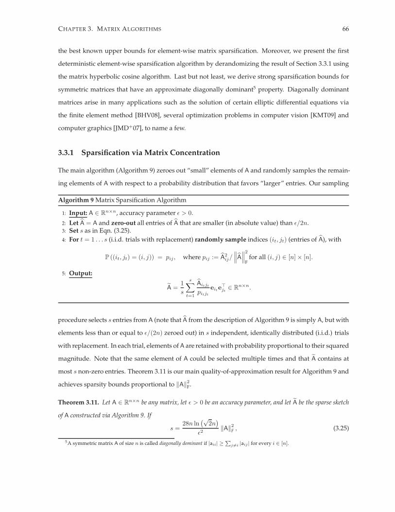
CHAPTER 3. MATRIX ALGORITHMS 66
the best known upper bounds for element-wise matrix sparsification. Moreover, we present the first
deterministic element-wise sparsification algorithm by derandomizing the result of Section 3.3.1 using
the matrix hyperbolic cosine algorithm. Last but not least, we derive strong sparsification bounds for
symmetric matrices that have an approximate diagonally dominant5 property. Diagonally dominant
matrices arise in many applications such as the solution of certain elliptic differential equations via
the finite element method [BHV08], several optimization problems in computer vision [KMT09] and
computer graphics [JMD+07], to name a few.
3.3.1 Sparsification via Matrix Concentration
The main algorithm (Algorithm 9) zeroes out “small” elements of A and randomly samples the remain-
ing elements of A with respect to a probability distribution that favors “larger” entries. Our sampling
Algorithm 9 Matrix Sparsification Algorithm
1: Input: A ∈ Rn×n, accuracy parameter ǫ > 0.
2: Let A = A and zero-out all entries of A that are smaller (in absolute value) than ǫ/2n.3: Set s as in Eqn. (3.25).
4: For t = 1 . . . s (i.i.d. trials with replacement) randomly sample indices (it, jt) (entries of A), with
P ((it, jt) = (i, j)) = pij , where pij := A2ij/∥∥∥A∥∥∥
2
Ffor all (i, j) ∈ [n]× [n].
5: Output:
A =1
s
s∑
t=1
Aitjt
pitjt
eite⊤jt∈ R
n×n.
procedure selects s entries from A (note that A from the description of Algorithm 9 is simply A, but with
elements less than or equal to ǫ/(2n) zeroed out) in s independent, identically distributed (i.i.d.) trials
with replacement. In each trial, elements of A are retained with probability proportional to their squared
magnitude. Note that the same element of A could be selected multiple times and that A contains at
most s non-zero entries. Theorem 3.11 is our main quality-of-approximation result for Algorithm 9 and
achieves sparsity bounds proportional to ‖A‖2F.
Theorem 3.11. Let A ∈ Rn×n be any matrix, let ǫ > 0 be an accuracy parameter, and let A be the sparse sketch
of A constructed via Algorithm 9. If
s =28n ln
(√2n)
ǫ2‖A‖2F , (3.25)
5A symmetric matrix A of size n is called diagonally dominant if |aii| ≥P
j 6=i |aij | for every i ∈ [n].

CHAPTER 3. MATRIX ALGORITHMS 67
then, with probability at least 1− n−1,∥∥∥A− A
∥∥∥2≤ ǫ.
A has at most s non-zero entries and the construction of A can be implemented in one pass over the input matrix
A (see Section 3.3.1).
We conclude this section with Corollary 3.12, which is a re-statement of Theorem 3.11 involving
the stable rank of A, denoted by sr (A) (recall that the stable rank of any matrix A is defined as the ratio
sr (A) := ‖A‖2F / ‖A‖22, which is upper bounded by the rank of A). The corollary guarantees relative error
approximations for matrices of – say – constant stable rank, such as the ones that arise in [Rec11, CT10].
Corollary 3.12. Let A ∈ Rn×n be any matrix and let ε > 0 be an accuracy parameter. Let A be the sparse sketch
of A constructed via Algorithm 9 (with ǫ = ε ‖A‖2). If s = 28n sr (A) ln(√
2n)/ε2, then, with probability at
least 1− n−1,∥∥∥A− A
∥∥∥2≤ ε ‖A‖2 .
It is worth noting that the sampling algorithm implied by Corollary 3.12 can not be implemented in
one pass, since we would need a priori knowledge of the spectral norm of A in order to implement Step
2 of Algorithm 9.
Randomized Element-wise Matrix Sparsification
Sparsity of eA Failure Citation CommentsProbability
ε > 4√
n · b16n ‖A‖2
F /ε2 + 84n log4 n Expected e−19 log4 n [AM07] n ≥ 700 · 106
n ≥ 1
R · b · n ‖A‖2F /ε2 Expected e−Ω(R·n) [GT09] ε > c1
√n · R · b
c2 ≤ 452
c2n log2“
n
log2 n
”
log n ‖A‖2F /ε2 Expected 1/n [NDT09b] ε > 0, n ≥ 300,
ε > 0, n ≥ 300
c3n log3 n ‖A‖2F /ε2 Expected 1/n [NDT10] Extends to tensors
c4√
nP
ij|Aij |/ε Exact e−Ω(n) [AHK06] ε > 0, n ≥ 1
14n ln (2n/δ) ‖A‖2F /ε2 Exact δ Thm 3.11 ε > 0, n ≥ 1
Table 3.1: Summary of prior results in element-wise matrix sparsification. The first column indicates the number
of non-zero entries in eA, whereas the second column indicates whether this number is exact or simply holds inexpectation. In terms of notation, we let b denote the maxi,j |Aij | and R denote maxij |Aij |/minAij 6=0 |Aij |. Finally,c1, c2, c3, c4 denote unspecified positive constants.

CHAPTER 3. MATRIX ALGORITHMS 68
Related Work. In this section (as well as in Table 3.1), we present a head-to-head comparison of our
result ([DZ11]) with all existing (to the best of our knowledge) bounds on randomized matrix spar-
sification. In [AM01, AM07] the authors presented a sampling method that requires in expectation
16n ‖A‖2F /ε2 + 84n log4 n non-zero entries in A in order to achieve an accuracy guarantee ε with a fail-
ure probability of at most e−19 log4 n. Compared with our result, their bound holds only when ε >
4√
n · maxi,j |Aij | and, in this range, our bounds are superior when ‖A‖2F /(maxi,j |Aij |)2 = o(n log3 n).
It is worth mentioning that the constant involved in [AM01, AM07] is two orders of magnitude larger
than ours and more importantly their results hold only when n ≥ 700 · 106.
In [GT09], the authors study the ‖·‖∞→2 and ‖·‖∞→1 norms in the matrix sparsification context and
they also present a sampling scheme analogous to ours. They achieve (in expectation) a sparsity bound
of Rn ‖A‖2F maxi,j |Aij | /ε2 when ε ≥√
nR maxi,j |Aij |; here R := maxij |Aij |/ minAij 6=0 |Aij |. Thus, our
results are superior (in the above range of ε) when R ·maxi,j |Aij | = ω(log n).
It is harder to compare our method to the work of [AHK06], which depends on the∑n
i,j=1 |Aij |. The
latter quantity is, in general, upper bounded only by n ‖A‖F, in which case the sampling complexity
of [AHK06] is much worse, namely O(n3/2 ‖A‖F /ε). Finally, the recent bounds on matrix sparsification
via the non-commutative Khintchine’s inequality in [NDT09b] are inferior compared to ours in terms
of sparsity guarantees by at least O(ln2(n/ ln2 n)). Nevertheless, we should mention that the bounds
of [NDT09b] can be extended to multi-dimensional matrices (tensors), whereas our result does not
generalize to this setting; see [NDT10] for details.
Background
Implementing the Sampling in one Pass over the Input Matrix. We now discuss the implementation
of Algorithm 9 in one pass over the input matrix A. Towards that end, we will leverage (a slightly
modified version of) Algorithm SELECT (p. 137 of [DKM06a]). We note that Step 3 essentially operates
Algorithm 10 One-pass SELECT algorithm
1: Input: aij for all (i, j) ∈ [n]× [n], arbitrarily ordered and ǫ > 0.2: N = 0.3: For all (i, j) ∈ [n]× [n] such that a2
ij > ǫ2
4n2
• N = N + a2ij .
• Set (I, J) = (i, j) and S = aij with probabilitya2ij
N .
4: Output: Return (I, J), S and N .
on A. Clearly, in a single pass over the data we can run in parallel s copies of the SELECT Algorithm
(using a total of O(s) memory) to effectively return s independent samples from A. Lemma 1 (page 136

CHAPTER 3. MATRIX ALGORITHMS 69
of [DKM06a], note that the sequence of the a2ij ’s is all-positive) guarantees that each of the s copies of
SELECT returns a sample satisfying:
P ((it, jt) = (i, j)) =A2
ij
∑ni,j=1 Aij
2 =A2
ij∥∥∥A∥∥∥
2
F
, for all t = 1, . . . , s.
Finally, in the parlance of Step 5 of Algorithm 9, (it, jt) is set to (I, J) and pitjtis set to S2/N for all
t ∈ [s].
Proof of Theorem 3.11 The proof of Theorem 3.11 will combine Lemmas 3.13 and 3.17 in order to
bound∥∥∥A− A
∥∥∥2
as follows:
∥∥∥A− A
∥∥∥2
=∥∥∥A− A + A− A
∥∥∥2≤∥∥∥A− A
∥∥∥2+∥∥∥A− A
∥∥∥2≤ ǫ/2 + ǫ/2 = ǫ.
The failure probability of Theorem 3.11 emerges from Lemma 3.17, which fails with probability at most
n−1 for the choice of s in Eqn. (3.25). The proof of Lemma 3.17 will involve the matrix-valued Bernstein
bound, see Chapter 1.
Bounding∥∥∥A− A
∥∥∥2
Lemma 3.13. Using the notation of Algorithm 9,∥∥∥A− A
∥∥∥2≤ ǫ/2.
Proof. Recall that the entries of A are either equal to the corresponding entries of A or they are set to
zero if the corresponding entry of A is (in absolute value) smaller than ǫ/(2n). Thus,
∥∥∥A− A
∥∥∥2
2≤∥∥∥A− A
∥∥∥2
F=
n∑
i,j=1
(A− A
)2
ij≤
n∑
i,j=1
ǫ2
4n2≤ ǫ2
4.
Bounding∥∥∥A− A
∥∥∥2
In order to prove our main result in this section (Lemma 3.17) we will leverage a powerful matrix-
valued Bernstein bound originally proven in [Rec11] (Theorem 3.2). We restate this theorem, slightly
rephrased to better suit our notation.
Theorem 3.14. [THEOREM 3.2 OF [REC11]] Let M1, M2, . . . , Ms be independent, zero-mean random matrices
in Rn×n. Suppose maxt∈[s]
∥∥E(MtM
⊤t
)∥∥2,∥∥E(M⊤
t Mt
)∥∥2
≤ ρ2 and ‖Mt‖2 ≤ γ for all t ∈ [s]. Then, for
CHAPTER 3. MATRIX ALGORITHMS 70
any τ > 0, ∥∥∥∥∥1
s
s∑
t=1
Mt
∥∥∥∥∥2
≤ τ
holds, subject to a failure probability of at most
2nexp
(− sτ2/2
ρ2 + γτ/3
).
In order to apply the above theorem, using the notation of Algorithm 9, we set Mt =bAitjt
pitjt
eite⊤jt− A
for all t ∈ [s] to obtain
1
s
s∑
t=1
Mt =1
s
s∑
t=1
[Aitjt
pitjt
eite⊤jt− A
]= A− A. (3.26)
It is easy to argue that E (Mt) = 0n for all t ∈ [s]. Indeed, if we consider that∑n
i,j=1 pij = 1 and
A =∑n
i,j=1 Aijeie⊤j we obtain
E (Mt) =
n∑
i,j=1
pij
(Aij
pijeie
⊤j − A
)=
n∑
i,j=1
Aijeie⊤j −
n∑
i,j=1
pijA = 0n.
Our next lemma bounds ‖Mt‖2 for all t ∈ [s].
Lemma 3.15. Using our notation, ‖Mt‖2 ≤ 4nǫ−1∥∥∥A∥∥∥
2
Ffor all t ∈ [s].
Proof. First, using the definition of Mt and the fact that pitjt= A2
itjt/∥∥∥A∥∥∥
2
F,
‖Mt‖2 =
∥∥∥∥∥Aitjt
pitjt
eite⊤jt− A
∥∥∥∥∥2
≤
∥∥∥A∥∥∥
2
F∣∣∣Aitjt
∣∣∣+∥∥∥A∥∥∥
2≤
2n∥∥∥A∥∥∥
2
F
ǫ+∥∥∥A∥∥∥
F.
The last inequality follows since all entries of A are at least ǫ/(2n) and the fact that∥∥∥A∥∥∥
2≤∥∥∥A∥∥∥
F. We
can now assume that
∥∥∥A∥∥∥
F≤
2n∥∥∥A∥∥∥
2
F
ǫ(3.27)
to conclude the proof of the lemma. To justify our assumption in Eqn. (3.27), we note that if it is violated,
then it must be the case that∥∥∥A∥∥∥
F< ǫ/(2n). If that were true, then all entries of A would be equal to
zero. (Recall that all entries of A are either zero or, in absolute value, larger than ǫ/(2n).) Also, if A
were identically zero, then (i) A would also be identically zero and, (ii) all entries of A would be at most
ǫ/(2n). Thus,∥∥∥A− A
∥∥∥2
= ‖A‖2 ≤ ‖A‖F ≤√
n2ǫ2
4n2=
ǫ
2.

CHAPTER 3. MATRIX ALGORITHMS 71
Thus, if the assumption of Eqn. (3.27) is not satisfied, the resulting all-zeros A still satisfies Theorem 3.11.
Our next step towards applying Theorem 3.14 involves bounding the spectral norm of the expectation
of MtM⊤t . The spectral norm of the expectation of M⊤
t Mt admits a similar analysis and the same bound
and is omitted.
Lemma 3.16. Using our notation,∥∥E(MtM
⊤t
)∥∥2≤ n
∥∥∥A∥∥∥
2
Ffor any t ∈ [s].
Proof. We start by evaluating E(MtM
⊤t
); recall that pij = A2
ij/∥∥∥A∥∥∥
2
F:
E(MtM
⊤t
)= E
((Aitjt
pitjt
eite⊤jt− A
)(Aitjt
pitjt
ejte⊤it− A⊤
))
=
n∑
i,j=1
pij
(Aij
pijeie
⊤j − A
)(Aij
pijeje
⊤i − A
⊤)
=n∑
i,j=1
(A2
ij
pijeie
⊤i − Aij Aeje
⊤i − Aijeie
⊤j A⊤ + pijAA⊤
)
=∥∥∥A∥∥∥
2
F
n∑
i=1
mi · eie⊤i −
n∑
j=1
Aej
n∑
i=1
Aije⊤i −
n∑
j=1
(n∑
i=1
Aijei
)(Aej
)⊤+
n∑
i,j=1
pijAA⊤,
where mi is the number of non-zeroes of the i-th row of A. We now simplify the above result using a
few simple observations:∑n
i,j=1 pij = 1, Aej = A(j),∑n
i=1 Aijei = A(j), and∑n
j=1 A(j)(A(j)
)⊤= AA⊤.
Thus, we get
E(MtM
⊤t
)=∥∥∥A∥∥∥
2
F
n∑
i=1
mi · eie⊤i −
n∑
j=1
A(j)(A(j)
)⊤−
n∑
j=1
A(j)(A(j)
)⊤+ AA⊤
=∥∥∥A∥∥∥
2
F
n∑
i=1
mi · eie⊤i − AA⊤.
Since 0 ≤ mi ≤ n and using Weyl’s inequality (Theorem 4.3.1 of [HJ90]), which states that by adding a
positive semi-definite matrix to a symmetric matrix all its eigenvalues will increase, we get that
−AA⊤ E(MtM
⊤t
) n
∥∥∥A∥∥∥
2
FIn.
Consequently∥∥E(MtM
⊤t
)∥∥2
= max
∥∥∥A∥∥∥
2
2, n∥∥∥A∥∥∥
2
F
= n
∥∥∥A∥∥∥
2
F.
We can now apply Theorem 3.14 on Eqn. (3.26) with τ = ǫ/2, γ = 4nǫ−1∥∥∥A∥∥∥
2
F(Lemma 3.15), and
ρ2 = n∥∥∥A∥∥∥
2
F(Lemma 3.16) . Thus, we get that
∥∥∥A− A
∥∥∥2≤ ǫ/2 holds, subject to a failure probability of

CHAPTER 3. MATRIX ALGORITHMS 72
at most
2nexp
− ǫ2s/8
(1 + 4/6)n∥∥∥A∥∥∥
2
F
.
Bounding the failure probability by δ and solving for s, we get that s ≥ 14ǫ2 n
∥∥∥A∥∥∥
2
Fln(
2nδ
). Using
∥∥∥A∥∥∥
F≤
‖A‖F (by construction) concludes the proof of the following lemma, which is the main result of this
section.
Lemma 3.17. Using the notation of Algorithm 9, if s ≥ 14nǫ−2 ‖A‖2F ln (2n/δ) , then, with probability at least
1− δ,∥∥∥A− A
∥∥∥2≤ ǫ/2.
3.3.2 Deterministic Matrix Sparsification
To the best of our knowledge, all known algorithms for this problem are randomized (see Table 3.1).
In this section, we present the first deterministic algorithm. A deterministic algorithm for the element-
wise matrix sparsification problem can be obtained by derandomizing Algorithm 9.
Theorem 3.18. Let A be an n × n matrix and 0 < ε < 1. There is a deterministic polynomial time algorithm
that, given A and ε, outputs a matrix A ∈ Rn×n with at most 28n ln(
√2n) sr (A) /ε2 non-zero entries such that
∥∥∥A− A
∥∥∥2≤ ε ‖A‖2 .
Proof. (of Theorem 3.18) By homogeneity, assume that ‖A‖2 = 1. Following the proof of Theorem 3.11,
we can assume that w.l.o.g. all non-zero entries of A have magnitude at least ε/(2n) in absolute value,
otherwise we can zero-out these entries and incur at most an error of ε/2.
Consider the bijection π between the sets [n2] and [n]×[n] defined by π(l) 7→ (⌈l/n⌉, (l−1) mod n+1)
for every l ∈ [n2]. Let Eij ∈ Rn×n be the all zeros matrix having one only in the (i, j) entry. Set
h(l) = D(
Aπ(l)
plEπ(l) − A
)where pl = A2
π(l)/ ‖A‖2F for every l ∈ [n2]. Observe that h(·) ∈ S2n×2n. Let
X be a random variable over [n2] with distribution pl, l ∈ [n2]. The same analysis as in Lemmas 3.15
and 3.16 of [DZ11] together with properties of the dilation map imply that ‖h(l)‖2 ≤ 4n sr (A) /ε for
every l ∈ [n2], E h(X) = 02n, and∥∥E h(X)2
∥∥2≤ n sr (A).
Run Algorithm 1 with h(·) as above. Algorithm 1 returns at most t = 28n ln(√
2n) sr (A) /ε2 indices
x∗1, x
∗2, . . . x
∗t over [n2] using O(n6 sr (A) log n/ε2) operations such that
∥∥∥∥∥1
t
t∑
l=1
h(x∗l )
∥∥∥∥∥2
≤ ε/2. (3.28)

CHAPTER 3. MATRIX ALGORITHMS 73
Set A := 1t
∑tl=1 Aπ(x∗
l)/px∗
lEπ(x∗
l). Observe that A has at most t non-zero entries. Now, by the definition
of h(·) and properties of the dilation map, it follows that Ineq. (3.28) is equivalent to∥∥∥D(A− A
)∥∥∥2
=∥∥∥A− A
∥∥∥2≤ ε/2.
3.3.3 Sparsification for SDD Matrices
In this section, we give an elementary connection between element-wise matrix sparsification and spec-
tral sparsification of psd matrices. A direct application of this connection implies strong sparsification
bounds for symmetric matrices that are close to being diagonally dominant. More precisely, we give two
element-wise sparsification algorithms for symmetric and diagonally dominant-like matrices; in its
randomized and the other in its derandomized version (see Table 3.1). Both algorithms share a crucial
difference with all previously known sampling-based algorithms for this problem; that is, during the
sparsification process they arbitrarily densify the diagonal entries. As we will see later this twist turns
out to allow strong sparsification bounds. The next theorem presents stronger sparsification algorithms
for the special case of diagonally dominant matrices both randomized and deterministic.
Theorem 3.19. Let A be any symmetric and diagonally dominant matrix of size n and 0 < ε < 1. Assume for
normalization that ‖A‖2 = 1.
(a) There is a randomized linear time algorithm that outputs a matrix A ∈ Rn×n with at most O(n log n/ε2)
non-zero entries such that, with probability at least 1− 1/n,∥∥∥A− A
∥∥∥2≤ ε.
(b) There is a deterministic O(ε−2 nnz (A)n2 log n maxlog2 n, 1/ε2) time algorithm that outputs a matrix
A ∈ Rn×n with at most O(n/ε2) non-zero entries such that
∥∥∥A− A
∥∥∥2≤ ε.
Recall that the results of [SS08, BSS09] imply an element-wise sparsification algorithm that works
only for Laplacian matrices. It is easy to verify that Laplacian matrices are also diagonally dominant.
Here we extend these results to a wider class of matrices (with a weaker notion of approximation). The
diagonally dominant assumption is too restrictive and we will show that our sparsification algorithms
work for a wider class of matrices. To accommodate this, we say that a matrix A is θ-symmetric diago-
nally dominant (abbreviate by θ-SDD) if A is symmetric and the inequality ‖A‖∞ ≤√
θ ‖A‖2 holds.
By definition, any diagonally dominant matrix is also a 4-SDD matrix. On the other extreme, every
symmetric matrix of size n is n-SDD since the inequality ‖A‖∞ ≤√
n ‖A‖2 is always valid. The fol-
lowing elementary lemma gives a connection between element-wise matrix sparsification and spectral
sparsification as defined in [Sri10].

CHAPTER 3. MATRIX ALGORITHMS 74
Lemma 3.20. Let A be a symmetric matrix of size n and R = diag (r1, r2, . . . , rn) where ri =∑
j 6=i |Aij |. Then
there is a matrix C of size n×m with m ≤(n2
)such that
A = CC⊤ + diag (A)− R. (3.29)
Moreover, each column of C is indexed by the ordered pairs (i, j), i < j and equals to C(i,j) =√|Aij |ei +
sign (Aij)√|Aij |ej for every i < j, i, j ∈ [n].
Proof. The key identity is CC⊤ :=∑
l,k∈[n], l<k C(l,k) ⊗ C(l,k). Let l, k ∈ [n] with l < k, it follows that
C(l,k) ⊗ C(l,k) =(√|Alk|el + sign (Alk)
√|Alk|ek
)(√|Alk|el + sign (Alk)
√|Alk|ek
)⊤
= |Alk|el ⊗ el + Alkek ⊗ ek + Alkek ⊗ el + |Alk|ek ⊗ ek.
Therefore
CC⊤ =∑
l,k∈[n]: l<k
[|Alk|el ⊗ el + Alkek ⊗ ek + Alkek ⊗ el + |Alk|ek ⊗ ek] . (3.30)
Let’s first prove the equality for the off-diagonal entries of Eqn (3.29). Let l < k and l, k ∈ [n]. By
construction, the only term of the sum that contributes to the (i, j) and (j, i) entry of the right hand side
of Eqn. (3.30) is the term C(i,j)⊗C(i,j). Moreover, this term equals |Aij |ei⊗ ei +Aijei⊗ ej +Aijej ⊗ ei +
|Aij |ej ⊗ ej . Since Aij = Aji this proves that the off-diagonal entries are equal.
For the diagonal entries of Eqn. (3.29), it suffices to prove that (CC⊤)ii = ri. First observe that
the last two terms of the sum in the right hand side of (3.30) do not contribute to any diagonal entry.
Second, the first two terms contribute only when l = i or k = i. In the case where l = i, the contribution
of the sum equals to∑
i<k |Aik|. On the other case (k = i), the contribution of the sum is equal to∑
l<i |Ali|. However, A is symmetric so Ali = Ail for every l < i. It follows that the total contribution is∑
i<k |Aik|+∑
l<i |Ail| =∑
j 6=i |Aij | = ri.
Remark 5. In the special case where A is the Laplacian matrix of some graph, the above decomposition is precisely
the vertex-edge decomposition of the Laplacian matrix, since in this case diag (A) = R.
Using the above lemma, we give a randomized and a deterministic algorithm for sparsifying θ-SDD
matrices. First we present the randomized algorithm.
Theorem 3.21. Let A be a θ-SDD matrix of size n and 0 < ε < 1. There is a randomized linear time algorithm
that, given A, ‖A‖2 and ε, outputs a matrix A ∈ Rn×n with at most O(nθ log n/ε2) non-zero entries such that
w.p. at least 1− 1/n,∥∥∥A− A
∥∥∥2≤ ε ‖A‖2 .

CHAPTER 3. MATRIX ALGORITHMS 75
Proof. In one pass over the input matrix A normalize the entries of A by ‖A‖2, so assume without loss
of generality that ‖A‖2 = 1. Let C be the n×m matrix guaranteed by Lemma 3.20, where m =(n2
), each
column of C is indexed by the ordered pairs (i, j), i < j and A = CC⊤ + diag (A) − R. By definition
of C and the hypothesis, we have that∥∥CC⊤∥∥
2= ‖A− diag (A) + R‖2 ≤ ‖A‖2 + ‖A‖∞ ≤ 2
√θ and
‖C‖2F = 2∑
i,j |Aij | ≤ 2n ‖A‖∞ ≤ 2n√
θ.
Consider the bijection between the sets [m] and (i, j) | i < j, i, j ∈ [n] defined by π(l) 7→ (⌈l/n⌉, (l−
1) mod n + 1). For each l ∈ [m], set pl =∥∥Cπ(l)
∥∥2
2/ ‖C‖2F and define f(l) := Cπ(l) ⊗ Cπ(l)/pl − CC⊤. Let
X be a real-valued random variable over [m] with distribution pl. It is easy to verify that E f(X) =
0n, ‖f(l)‖2 ≤ 2 ‖C‖2F for every l ∈ [m]. A direct calculation gives that∥∥E f(X)2
∥∥2≤ 2 ‖C‖2F
∥∥CC⊤∥∥2.
Matrix Bernstein inequality (see [Tro11b]) with f(·) as above (γ = 4n√
θ and ρ2 = 8nθ) tells us that if
we sample t = 38nθ ln(√
2n)/ε2 indices x∗1, x
∗2, . . . , x
∗t over [m] then with probability at least 1 − 1/n,
∥∥∥1t
∑tj=1 f(x∗
j )∥∥∥
2≤ ε. Now, set C ∈ R
n×t where the j-th column of C(j) equals 1√tCπ(x∗
j ). It follows that∥∥∥1
t
∑tj=1 f(x∗
j )∥∥∥
2=∥∥∥1
t
∑tj=1 Cπ(x∗
j ) ⊗ Cπ(x∗j ) − CC⊤
∥∥∥2
=∥∥∥CC⊤ − CC⊤
∥∥∥2. Define A = CC⊤+diag (A)−R.
First notice that∥∥∥A− A
∥∥∥2
=∥∥∥CC⊤ − CC⊤
∥∥∥2≤ ε. It suffices to bound the number of non-zeros of A. To
do so, view the matrix-product CC⊤ as a sum of rank-one outer-products over all columns of C. By the
special structure of the entries of C, every outer-product term of the sum contributes to at most four
non-zero entries, two of which are off-diagonal. Since C has at most t columns, A has at most n + 2t
non-zero entries; n for the diagonal entries and 2t for the off-diagonal.
Next we state the derandomized algorithm of the above result.
Theorem 3.22. Let A be a θ-SDD matrix of size n and 0 < ε < 1/2. There is an algorithm that, given A and ε,
outputs a matrix A ∈ Rn×n with at most O(nθ/ε2) non-zero entries such that
∥∥∥A− A
∥∥∥2≤ ε ‖A‖2. Moreover,
the algorithm computes A in deterministic O(nnz (A)n2θ log3 n/ε2 + n4θ2 log n/ε4) time.
Remark 6. The results of [BSS09, Sri10] imply a deterministic O(nnz (A) θn3/ε2) time algorithm that outputs
a matrix A with at most ⌈19(1 +√
θ)2/ε2⌉n non-zero entries such that∥∥∥A− A
∥∥∥2≤ ε ‖A‖2.
Proof. Let C be the n × m matrix such that A = CC⊤ + diag (A) − R and m ≤ nnz (A) guaranteed by
Lemma 3.20. Apply Theorem 3.10 on the matrix CC⊤ and ε which outputs, in deterministic O(nnz (A) n2
θ log3 n/ε2 + n4θ2 log n/ε4) time, an n × ⌈n/ε2⌉ matrix C such that (1 − ε)3CC⊤ CC⊤ (1 + ε)3CC⊤.
By Weyl’s inequality [HJ90, Theorem 4.3.1] and the fact that ε < 1/2, it follows that∥∥∥CC⊤ − CC⊤
∥∥∥2≤
5ε∥∥CC⊤∥∥
2. Define A := CC⊤ + diag (A) − R. First we argue that the number of non-zero entries of A
is at most n + ⌈2n/ε2⌉. Recall that every column of C is a rescaled column of C. Now, think the matrix-
product CC⊤ as a sum of rank-one outer-products over all columns of C. By the special structure of the

CHAPTER 3. MATRIX ALGORITHMS 76
entries of C, every outer-product term of the sum contributes to at most four non-zero entries, two of
which are off-diagonal. Since C has at most ⌈n/ε2⌉ columns, A has at most n+ ⌈2n/ε2⌉ non-zero entries;
n for the diagonal entries and ⌈2n/ε2⌉ for the off-diagonal. Moreover, A is close to A in the operator
norm sense. Indeed,
∥∥∥A− A
∥∥∥2
=∥∥∥CC
⊤ − CC⊤∥∥∥
2≤ 5ε
∥∥CC⊤∥∥
2= 5ε ‖A− diag (A) + R‖2
≤ 5ε(‖A‖2 + ‖A‖∞) ≤ 10ε√
θ ‖A‖2
where we used the definition of A, Eqn. (3.29), triangle inequality, the assumption that A is θ-SDD and
the fact that θ ≥ 1. Repeating the proof with ε′ = ε10
√θ
and elementary manipulations conclude the
proof.

Chapter 4Graph Algorithms
In the present chapter1, we discuss applications of the tools analyzed in the previous chapters to graph
theoretic problems. More precisely, we discuss three problems: (i) the construction of expanding Cayley
graphs, (ii) an efficient deterministic algorithm for graph sparsification, and (iii) randomized gossip
algorithms for solving Laplacian systems.
4.1 Alon-Roichman Expanding Cayley Graphs
The Alon-Roichman theorem asserts that Cayley graphs obtained by choosing a logarithmic num-
ber of group elements independently and uniformly at random are expanders [AR94]. The origi-
nal proof of Alon and Roichman is based on Wigner’s trace method, whereas recent proofs rely on
matrix-valued deviation bounds [LR04]. Wigderson and Xiao’s derandomization of the matrix Cher-
noff bound implies a deterministic O(n4 log n) time algorithm for constructing Alon-Roichman graphs.
Independently, Arora and Kale generalized the multiplicative weights update (MWU) method to the
matrix-valued setting and, among other interesting implications, they improved the running time to
O(n3 polylog (n)) [Kal07]. Here we further improve the running time to O(n2 log3 n) by exploiting the
group structure of the problem. In addition, our algorithm is combinatorial in the sense that it only
requires counting the number of all closed (even) paths of size at most O(log n) in Cayley graphs. All
previous algorithms involve numerical matrix computations such as eigenvalue decompositions and
matrix exponentiation.
We start by describing expander graphs. Given a connected undirected d-regular graph H = (V, E)
1Both sections 4.1 and 4.2 appeared in [Zou12]. A preliminary version of Section 4.3 appeared in [FZ12] (joint work with NickFreris).
77
CHAPTER 4. GRAPH ALGORITHMS 78
on n vertices, let A be its adjacency matrix, i.e., Aij = wij where wij is the number of edges between
vertices i and j. Moreover, let A := 1dA be its normalized adjacency matrix. We allow self-loops and
multiple edges. Let λ1(A), . . . , λn(A) be its eigenvalues in decreasing order. We have that λ1(A) = 1
with corresponding eigenvector 1/√
n, where 1 is the all-one vector. The graph H is called a spectral
expander if λ(A) := max2≤j|λj(A)| ≤ ε for some positive constant ε < 1.
Denote by mk = mk(H) := tr(Ak). By definition, mk is equal to the number of self-returning walks
of length k of the graph H . A graph-spectrum-based invariant, proposed by Estrada is defined as
EE(A) := tr (exp [A]) [ERV05], which also equals to∑∞
k=0 mk/k!. For θ > 0, we define the even θ-Estrada
index by EEeven(A, θ) :=∑∞
k=0 m2k(θA)/(2k)!.
Now let G be any finite group of order n with identity element id. Let S be a multi-set of elements
of G, we denote by S ⊔S−1 the symmetric closure of S, namely the number of occurrences of s and s−1
in S ⊔ S−1 equals the number of occurrences of s ∈ S. Let R be the right regular representation2, i.e.,
(R(g1)φ)(g2) = φ(g1g2) for every φ : G→ R and g1, g2 ∈ G. The Cayley graph Cay (G; S) on a group G
with respect to the mutli-set S ⊂ G is the graph whose vertex set is G, and where g1 and g2 are connected
by an edge if there exists s ∈ S such that g2 = g1s (allowing multiple edges for multiple elements in S).
In this section we prove the correctness of the following greedy algorithm for constructing expanding
Cayley graphs.
Theorem 4.1. Given the multiplication table of a finite group G of size n and 0 < ε < 1, Algorithm 11
outputs a (symmetric) multi-set S ⊂ G of size O(log n/ε2) such that λ(Cay (G; S)) ≤ ε in O(n2 log3 n/ε5)
time. Moreover, the algorithm performs only group algebra operations that correspond to counting closed paths
in Cayley graphs.
Remark 7. To the best of our knowledge, the above theorem improves the running time of all previously known
deterministic constructions of Alon-Roichman Cayley graphs [AK07, WX08, Kal07], see also [AMN12] for an
alternative polynomial time construction. Moreover, notice that the running time of the above algorithm is
optimal up-to poly-logarithmic factors since the size of the multiplication table of a finite group of size n isO(n2).
Let A be the normalized adjacency matrix of Cay(G; S ⊔ S−1
)for some S ⊂ G. It is not hard to
see that A = 12|S|
∑s∈S (R(s) + R(s−1)). We want to bound λ(A). Notice that λ(A) = ‖(I− J/n)A‖2.
Since we want to analyze the second-largest eigenvalue (in absolute value), we consider (I − J/n)A =
1|S|∑
s∈S (R(s) + R(s−1))/2 − J/n. Based on the above calculation, we define our matrix-valued func-
tion as
f(g) := (R(g) + R(g−1))/2 − J/n (4.1)
2In other words, represent each group algebra element with a permutation matrix of size n that preserves the group structure.This is always possible due to Cayley’s theorem.

CHAPTER 4. GRAPH ALGORITHMS 79
Algorithm 11 Expander Cayley Graph via even Estrada Index Minimization
1: procedure GREEDYESTRADAMIN(G, ε) ⊲ Multiplication table of G, 0 < ε < 12: Set S(0) = ∅ and t = O(log n/ε2)3: for i = 1, . . . t do4: Let g∗ ∈ G that (approximately) min. the even ε/2-Estrada index of Cay
(G; S(i−1) ∪ g ∪ g−1
)
over all g ∈ G ⊲ Use Lemma 4.35: Set S(i) = S(i−1) ∪ g∗ ∪ g−1
∗6: end for7: Output: A multi-set S := S(t) of size 2t such that λ(Cay (G; S)) ≤ ε8: end procedure
for every g ∈ G. The following lemma connects the potential function that is used in Theorem 1.19 and
the even Estrada index.
Lemma 4.2. Let S ⊂ G and A be the adjacency matrix of Cay(G; S ⊔ S−1
). For any θ > 0, tr
(cosh
[θ∑
s∈S f(s)])
=
EEeven(A, θ/2) + 1− cosh(θ|S|).
Proof. For notational convenience, set P := In − Jn/n and B := θ2
∑s∈S(R(s) + R(s)−1). Since JR(g) =
R(g)J = J, we have that tr(
cosh[θ∑
s∈S f(s)])
= tr (cosh [PB]). Now using Lemma 1.5, it follows
tr (cosh [PB]) = tr (P cosh [B] + I− P) = tr (cosh [B]) + tr(−J
n cosh [B] + I− P). Notice that J/n is a projec-
tor matrix, hence applying Lemmata 1.3 and 1.5 we get that
tr
(−J
ncosh [B] + I− P
)= tr (− cosh [J/nB] + P + I− P) = 1− cosh(θ|S|).
The following lemma indicates that it is possible to efficiently compute the (even) Estrada index for
Cayley graphs with small generating set.
Lemma 4.3. Let S ⊂ G, θ, δ > 0, and A be the adjacency matrix of Cay (G; S). There is an algorithm that,
given S, computes an additive δ approximation to EE(θA) or EEeven(A, θ) in O(n|S|maxlog(n/δ), 2e2|S|θ)
time.
Proof. We will prove the Lemma for EE(A, θ), the other case is similar. Let h := θ∑
s∈S s be a group
algebra element of G, i.e, h ∈ R[G]. Define exp [h] := id+∑∞
k=1h⋆k
k! and Tl(h) := id+∑l
k=1h⋆k
k! (where
h⋆k is the k-folded convolution/multiplication over R[G]) the exponential operator and its l truncated
Taylor series, respectively. Notice that θA = θ∑
s∈S R(s) = R(h), so EE(A, θ) = tr (exp [R(h)]) =
tr (R(exp [h])). We will show that the quantity tr (R(Tl(h))) is a δ approximation for EE(A, θ) when
l ≥ maxlog(n/δ), 2e2|S|θ.

CHAPTER 4. GRAPH ALGORITHMS 80
Compute the sum of Tl(h) by summing each term one by one and keeping track of all the coef-
ficients of the group algebra elements. The main observation is that at each step there are at most
n such coefficients since we are working over R[G]. For k > 1, compute the k-th term of the sum by
(∑
s∈S css)k/k! = (
∑s∈S css)
k−1/(k−1)!·∑s∈S(cs/k)s. Assume that we have computed the first term of
the above product, which is some group algebra element denote it by∑
g∈G βgg for some βg ∈ R. Hence,
at the next iteration, we have to compute the product/convolution of∑
g∈G βgg with θ/k∑
s∈S s, which
can be done in O(n|S|) time. Since the sum has l terms, in total we require O(n|S|l) operations. Now,
we show that it is a δ approximation. We need the following fact (see [Hig08, Theorem 10.1, p. 234])
Fact 4.4. For any B ∈ Rn×n, let Tl(B) :=
∑lk=0
Bk
k! . Then, ‖exp [B]− Tl(B)‖2 ≤‖B‖l+1
2
(l+1)! e‖B‖2 .
Notice that ‖θA‖2 =∥∥∑
s∈S θR(s)∥∥
2≤ θ|S| by triangle inequality and the fact that ‖R(g)‖2 = 1 for
any g ∈ G. Applying Fact 4.4 on θA we get that
‖exp [θA]− Tl(θA)‖2 ≤(θ|S|)l+1
(l + 1)!eθ|S| ≤
(eθ|S|l + 1
)l+1
eθ|S|
=
(e1+(θ|S|)/(l+1)θ|S|
l + 1
)l+1
≤ 1
2l+1≤ δ
n.
where we used the inequality (l + 1)! ≥ ( l+1e )l+1 and the assumption that l ≥ maxlog(n/δ), 2e2θ|S|.
Proof. (of Theorem 4.1) By Lemma 4.2, minimizing the even ε/2-Estrada index in the i-th iteration is
equivalent to minimizing tr(
cosh[θ∑
s∈S(i−1) f(s) + θf(g)])
over all g ∈ G with θ = ε. Notice that
f(g) ∈ Sn×n for g ∈ G, Eg∈RG f(g) = 0n since∑
g∈G R(g) = J. It is easy to see that ‖f(g)‖2 ≤ 2 and
moreover a calculation implies that∥∥Eg∈RG f(g)2
∥∥2≤ 2 as well. Theorem 1.19 implies that we get a
multi-set S of size t such that λ(Cay(G; S ⊔ S−1
)) =
∥∥∥ 1|S|∑
s∈S f(s)∥∥∥
2≤ ε. The moreover part follows
from Lemma 4.3 with δ = eε2
nc for a sufficient large constant c > 0. Indeed, in total we incur (following
the proof of Theorem 1.19) at most an additive ln(δneε2t)/ε error which is bounded by ε.
4.2 Deterministic Graph Sparsification
The second problem that we study is the graph sparsification problem. This problem poses the question
whether any dense graph can be approximated by a sparse graph under different notions of approxima-
tion. Given any undirected graph, the most well-studied notions of approximation by a sparse graph
include approximating, (i) all pairwise distances up to an additive error [PS89], (ii) every cut to an arbi-
trarily small multiplicative error [BK96] and (iii) every eigenvalue of the difference of their Laplacian

CHAPTER 4. GRAPH ALGORITHMS 81
matrices to an arbitrarily small relative error [Spi10]; the resulting graphs are usually called graph span-
ners, cut sparsifiers and spectral sparsifiers, respectively. Given that the notion of spectral sparsification is
stronger than cut sparsification, we focus on spectral sparsifiers. An efficient randomized algorithm to
construct an (1 + ε)-spectral sparsifier with O(n log n/ε2) edges was given in [SS08]. Furthermore, an
(1+ε)-spectral sparsifier withO(n/ε2) edges can be computed inO(mn3/ε2) deterministic time [BSS09].
The latter result is a direct corollary of the spectral sparsification of positive semi-definite (psd) matri-
ces problem as defined in [Sri10]; see also [Nao11b] for more applications. For additional references,
see [FHHP11]. Here we present an efficient deterministic spectral graph sparsification algorithm for
the case of dense graphs.
Let us formalize the notion of cut and spectral sparsification. Let G = (V, E, we) be a connected
weighted undirected graph with n vertices, m edges and edge weights we ≥ 0. Spectral sparsification
was inspired by the notion of cut3 sparsification introduced by Benczur and Karger [BK96] to accelerate
cut algorithms whose running time depends on the number of edges. They designed algorithms that,
given G and a parameter ε > 0, output a weighted subgraph G = (V, E, we) with |E| = O(n log n/ε2)
such that
∀S ⊆ V, (1− ε)∑
(S,S)∋e∈E
we ≤∑
(S,S)∋e∈ eE
we ≤ (1 + ε)∑
(S,S)∋e∈E
we. (4.2)
We call such a graph G, an (1 + ε)-cut sparsifier of G. Let L and L be the Laplacian matrices of G and
G, respectively. Condition (4.2) can be expressed using the language of Laplacians as follows
(1− ε)x⊤Lx ≤ x⊤Lx ≤ (1 + ε)x⊤Lx, for all x ∈ 0, 1n. (4.3)
Spielman and Teng [ST11] devised stronger sparsifiers that extend (4.3) to all x ∈ Rn, but required
O(n logc n) edges for a large constant c. Quite recently, Spielman and Srivastava [SS08] constructed
sparsifiers with O(n log n/ε2) that satisfy
(1− ε)x⊤Lx ≤ x⊤Lx ≤ (1 + ε)x⊤Lx, for all x ∈ Rn. (4.4)
We say that G is an (1 + ε)-spectral sparsifier of G, if it satisfies Ineq. (4.4).
The latter result of Spielman and Srivastava [SS08] implicitly4 used the matrix Bernstein inequal-
ity (Theorem 1.15). In particular, they proved a stronger statement: they showed that there exists a
3Let S ⊆ V . A cut, denoted by (S, S), is a partition of the vertices of a graph into two disjoint subsets S and S. The cut-set ofthe cut is the set of edges whose end points are in different subsets of the partition. The weight of a cut equals to the sum of theweights of all distinct edges contained in the cut-set.
4To be precise, they used Vershynin and Rudelson’s matrix Chernoff bound [RV07], however the same bound follows via thematrix Bernstein bound as was noticed in [Zou11].

CHAPTER 4. GRAPH ALGORITHMS 82
probability distribution over the edges of any graph G, so that sampling O(n log n/ε2) edges with re-
placement will result to a sub-graph of G that satisfies Ineq. (4.4) with high probability. They also gave a
nearly-linear time algorithm for constructing such spectral sparsifiers. Furthermore, an (1 + ε)-spectral
sparsifier with O(n/ε2) edges can be computed in O(mn3/ε2) deterministic time [BSS09]. In a recent
paper, the author obtained a faster deterministic algorithm than [BSS09] for the case of dense graphs
and constant ε. This was achieved by combining the matrix hyperbolic cosine algorithm (Algorithm 1)
together with tools from numerical linear algebra such as the Fast Multipole Method and fast solvers
for special type of eigensystems.
Theorem 4.5. Given a weighted graph G = (V, E) on n vertices, Ω(n2) edges with positive weights and
0 < ε < 1, there is a deterministic algorithm that returns an (1 + ε)-spectral sparsifier with O(n/ε2) edges in
O(n4 log n/ε2 maxlog2 n, 1/ε2) time.
The proof is a direct corollary of the fast deterministic isotropic sparsification algorithm, Algo-
rithm 8. The reduction from graph sparsification to sparsification of vectors in isotropic position was
first observed in [BSS09, Sri10].
Proof. Given the weighted Laplacian matrix L =∑
(i,j)∈E w(i,j)b(i,j) ⊗ b(i,j) where the i-th coordi-
nate of b(i,j) equals to 1, the j-th equals to −1, and zero otherwise. Theorem 3.10 with input the
vectors √webee∈E , outputs a set of positive weights see∈E (at most O(n/ε2) of them are positive)
in O(mn2 log3 n/ε2 + n4 log n/ε4) time so that
(1 − ε)L ∑
e∈E
sewebe ⊗ be (1 + ε)L.
It follows that the induced subgraph by the non-zero weights sewee∈E is an (1+ ε)-spectral sparsifier
of G having at most O(n/ε2) edges.
4.3 Randomized Gossip Algorithms for Solving Laplacian Systems
We present distributed algorithms for solving Laplacian systems under the gossip model of computa-
tion (a.k.a. asynchronous time model) [BGPS06], for earlier references on the gossip model see [TBA86,
BT89]. The proposed algorithms are based on the randomized Kaczmarz and the randomized extended
Kaczmarz algorithms that have been discussed in Section 3.1.2. To the best of our knowledge, the con-
nection between the gossip model of computation and Kaczmarz-like algorithms was first observed
in [FZ12] and will be discussed in Section 4.3.4. In Section 4.3.5, we present an improved gossip al-

CHAPTER 4. GRAPH ALGORITHMS 83
gorithm by exploiting the special structure of Laplacian matrices for the case of solvable Laplacian
systems.
4.3.1 The Model of Computation: Gossip algorithms
The gossip model of computation is also known in the literature as asynchronous time model [TBA86,
BT89]. Gossip algorithms can be categorized as being randomized or deterministic. Here, we focus on
the randomized gossip model (from now on we will drop the adjective randomized). The gossip model
is, roughly speaking, defined as the classical asynchronous model of computation enriched with the
additional assumption that each node can activate itself randomly in a fixed (pre-decided) rate. The
model implicitly assumes that the computational power of all nodes is comparable with each other.
More formally, the gossip model is defined as follows: Each node i has a clock which ticks at the
times of a γi Poisson process5. The model implicitly assumes that the clocks over all nodes of the net-
work run with the same speed (no clock drift). The inter-tick times of each node are rate γi exponential
random variables, independent over all the nodes and over time. Equivalently, using properties of the
Poisson distribution6, this corresponds to a single (global) clock ticking with a rate∑
i∈V γi Poisson
time process at times Z0, Z1, Z2, . . ., where Zk −Zk−1 are i.i.d. exponentials of rate γIkassuming that
node Ik ∈ V is selected at the k-th tick. It is easy to see that Ik are i.i.d. random variables distributed
over V with probability mass γii∈V .
A Chernoff bound type of argument can be used to relate the number of clock ticks to absolute
time (time units) which allows us to discuss the results in terms of clock ticks instead of absolute time,
see [BGPS06] for the details. Therefore, the algorithmic design problem under the gossip model is to
analyze distributed algorithms that require the minimum possible number of clock ticks in expectation
given a particular problem.
4.3.2 Related Work
The earliest reference in gossip or epidemic algorithms is the work of Demers et al. [DGH+87] in which
they first coined the term “gossip”, see also [Pit87]. The authors in [DGH+87] proposed gossip algo-
rithms for maintaining up-to-date replicates over a network of databases.
One of the most studied problem in distributed computation is the average consensus problem,
i.e., initially each node receives a value and each node should compute the average over all the node
5See [Fel66] for a detailed discussion about Poisson processes.6Let W1, . . . , Wn be n independent exponential random variables with rates γ1, . . . , γn, respectively. Let Wmin be the mini-
mum of W1, . . . , Wn. Then Wmin is an exponential random variable of ratePn
i=1 γi.
CHAPTER 4. GRAPH ALGORITHMS 84
values. The analysis of classical (synchronous and asynchronous) distributed algorithms for the aver-
aging problem can be traced back to [TBA86]. The work of Karp et al. [KSSV00] presented a general
lower bound for the averaging problem for any graph and any gossip algorithm in the synchronous
setting. Gossip-based algorithms for aggregating information where the underlying graph is the com-
plete graph was studied in [KDG03], see also [KDN+06] for improvements. The analysis of random-
ized gossip-based averaging algorithms for an arbitrarily network topology was studied in [BGPS04,
BGPS06]. Although the results of [BGPS06] are stated for computing the average function, their theo-
retical framework can be easily extended to the computation of other functions as well including the
maximum, the minimum or product functions of the node values.
Solving Laplacian systems in a distributed manner is also a fundamental computational primitive
since several problems can be formulated as the solution of a Laplacian system such as the clock
synchronization problem over a network [GK11, EKPS04, FZ12]. Laplacian solvers have been ana-
lyzed in both the synchronous and asynchronous model of distributed computation using for example
the synchronous and asynchronous Jacobi iteration [TBA86]. On the other hand, to the best of our
knowledge, the design of Laplacian solvers under the gossip model of computation has not been well-
studied. Nevertheless, the techniques of [BGPS06] have been extended to provide an algorithm that
converges to a solution of any given Laplacian system [BDFSV10, XBL05, XBL06], for additional ref-
erences see [DKM+10, § IV]. The underlying idea of [BDFSV10, XBL05, XBL06] is to use the average
consensus algorithms of [BGPS06] as the main building block to solve Laplacian systems. The follow-
ing theorem summarizes7 the outcome of these approaches (see the following section for notation).
Theorem 4.6. [BDFSV10, Theorem 5] Let G = (V, E) be a connected network of n nodes and assume that
each node i ∈ V gets as input a value bi. There is a consensus-based algorithm so that: every node i ∈ V
asymptotically computes the i-th entry of the vector xLS, where xLS is the minimum ℓ2-norm solution vector of the
Laplacian system L(G)x = b.
We are not aware of any algorithmic results in the literature similar to the above theorem that also
provide bounds on the rate of convergence. The main purpose of this section is to present a distributed
Laplacian solver under the gossip model of computation with exponential convergence in expectation,
see Corollary 4.8.
7We should mention that the approaches of [BDFSV10, XBL05, XBL06] operate under a more general setting of time-varyingnetwork topologies requiring only weak conditions of connectivity [XBL06].

CHAPTER 4. GRAPH ALGORITHMS 85
4.3.3 Preliminaries and Problem Definition
The communication network is modeled by an undirected graph G = (V, E). We let n := |V | be
the number of nodes/agents and m := |E| be the number of communication links. For simplicity,
communication is taken symmetric and moreover we assume that there are no communication failures.
Two neighboring nodes i, j : (i, j) ∈ E, can exchange packets to share information.
Let us label the nodes as 1, . . . , n and write the undirected edge e = (i, j) with i < j. Consider any
unknown vector x ∈ Rn of node variables, where variable xi corresponds to node i. The edge-vertex
incidence matrix of the graph B ∈ Rm×n has entries:
Bek :=
−1, if k = i;
1, if k = j;
0, otherwise.
(4.5)
Let L be the unnormalized Laplacian matrix of G, i.e., L = D − A where A is the adjacency matrix of
G and D is the diagonal matrix whose (i, i)-th entries is the degree of node i. It is a well-known fact
that L = B⊤B. The goal of this section is to design distributed algorithms under the gossip model of
computation that solve
Lx = b.
We assume that every node i ∈ V has access only to the values bi and bj for all j that are adjacent to
i. Since L is singular Lx = b may have no solution, therefore the goal is to compute, in a distributed
manner, the entries of the minimum ℓ2-norm least squares solution, xLS := L†b. More precisely, each
node i ∈ V has to compute (actually sufficiently approximate) the i-th coefficient of xLS.
Basics from graph theory For each i ∈ V , we define its neighborhood, Ni := j ∈ V : (i, j) ∈
E or (j, i) ∈ E. The degree of the node is di := |Ni|, and we define dmax := maxi di. Let λ1 ≤
λ2 ≤ . . . ≤ λn be the eigenvalues of L. For a connected graph we have that λ1 = 0, and 0 < λi ≤ dmax,
for i = 2, . . . , n. The second smallest eigenvalue of L denoted by λ2(G), also called the Fiedler value or
algebraic connectivity of G, can be lower-bounded via Cheeger’s inequality [Chu97] as follows: define for
each non-empty S ⊆ V , the volume to be the sum of the degrees of the vertices in S: vol(S) :=∑
i∈S di;
furthermore, let E(S, S) be the set of edges with one vertex in S and the other one in V \ S; finally, let
hG(S) := |E(S,S)|minvol(S),vol(S) . The Cheeger constant of G is defined as hG := minS 6=∅ hG(S). Then:
λ2(G) ≥ h2G
2dmax. (4.6)

CHAPTER 4. GRAPH ALGORITHMS 86
We will show that the expected rate of convergence of the proposed random gossip algorithms depends
on λ2(G). From now on we implicitly assume that that input graph is connected.
Let B = UΣV⊤ be the (truncated) singular value decomposition of B, i.e., U and V are m × (n − 1)
and n × (n − 1) matrices with orthonormal columns respectively, and Σ is a diagonal matrix of size
(n− 1) with positive elements. Since L = B⊤B, it holds that L = VΣ2V⊤.
Basics from Linear Algebra We summarize an observation regarding the structure of the minimum
ℓ2-norm least-squares solution of Laplacian systems.
Lemma 4.7. Let xLS be the minimum ℓ2-norm least squares solution of Lx = b. Let x′LS
be the returned vector
after the following two-step procedure:
(a) Compute the minimum ℓ2-norm least squares solution of B⊤y = b, i.e., yLS := (B⊤)†b
(b) Compute and return the minimum ℓ2-norm least squares solution of Bx = yLS, i.e., x′LS
:= B†yLS
Then, x′LS equals xLS.
Proof. Notice that x′LS
= B†yLS = B†(B⊤)†b = VΣ−1U⊤UΣ−1V⊤b = VΣ−2V⊤b = L†b where we used
that B = UΣV⊤, U⊤U = I(n−1) and VΣ−2V⊤ = L†.
4.3.4 Randomized Gossiping via Randomized Extended Kaczmarz
We propose a randomized gossip algorithm that exponentially converges to the least-squares solution
of the Laplacian system corresponding to the underlying communication graph. The proposed gos-
sip algorithm is based on the randomized extended Kaczmarz method (Algorithm 7) as explained in
detail next. Namely, we translate the randomized extended Kaczmarz algorithm (Algorithm 7) to a
distributed Laplacian solver under the gossip model of computation.
Consider a given column of L with index j ∈ [n]. L(j) has dj +1 non-zero entries whose off-diagonal
entries are equal to −1 and its diagonal entry equals to dj , so∥∥L(j)
∥∥2
2= d2
j + dj . Moreover for any
z ∈ Rn we have
⟨z, L(j)
⟩= djzj −
∑l∈Nj
zl. Step 6 of Algorithm 7 is translated to
z(k+1) ← z(k) +z(k)j − 1
dj
∑l∈Nj
z(k)l
dj + 1L(j).
In particular, if j ∈ V is selected the only coordinates of z that are updated are (zl)l∈Nibeause of
the sparsity of L(j). This part of the algorithm is clearly distributed in the sense that only the one-
hop neighbors of i make updates of their local estimates based solely on exchanging their previous
estimates.

CHAPTER 4. GRAPH ALGORITHMS 87
Similarly, consider a given row of L, say i ∈ [n], then for any x ∈ Rn we have
⟨x, L(i)
⟩= dixi −
∑l∈Ni
xl as before. Step 7 of Algorithm 7 is translated to
x(k+1) ← x(k) +(bi − z
(k)i )/di − x
(k)i − 1
di
∑l∈Ni
x(k)i
di + 1L(i).
Again, the above step can be implemented in a distributed setting, see Step 10 to Step 12 of Algo-
rithm 12. Putting all the above observations together, we end up with Algorithm 12. This algorithm
has exponential convergence in expectation as it almost immediately follows from Theorem 3.6, and its
rate of convergence depends solely on the topology of the underlying communication network.
Algorithm 12 Randomized Gossip Laplacian Solver
1: procedure2: for all nodes i ∈ V do ⊲ Initialization step
3: Set x(0)i = 0 and detect neighbors Ni
4: Node i obtains bj for all j ∈ Ni (hypothesis)
5: Set z(0)i = bi
6: end for7: for k = 0, 1, 2, . . . (each clock tick) do8: Pick a node ik ∈ V with probability proportional d2
ik+ dik
9: Node ik collects x(k)j and z
(k)j from all its neighbors j ∈ Ni
10: Node ik broadcasts: θ := z(k)ik− 1
dik
∑l∈Nik
z(k)l and ξ := (bik
−z(k)ik
)/dik+x
(k)ik− 1
dik
∑l∈Nik
x(k)l
11: Node ik sets: z(k+1)ik
← z(k)ik
+dik
θ
1+dik
and x(k+1)ik
← x(k)ik
+dik
ξ
1+dik
12: Every node j ∈ Niksets: z
(k+1)j ← z
(k)j − θ
1+dik
and x(k+1)j ← x
(k)j − ξ
1+dik
13: end for14: end procedure
Corollary 4.8 (Convergence rate of Algorithm 12). The updates of estimates produced by Algorithm 12
satisfy:
E
∥∥∥x(k) − xLS
∥∥∥2
2≤(
1− λ22(G)
2∑
i d2i + di
)⌊k/4⌋ (‖xLS‖22 + 2 ‖b‖22 /λ2
2(G))
.
In particular, for any ε > 0, if k ≥ 8P
id2
i +di
λ22(G)
ln(
‖xLS‖22+2‖b‖2
2/λ22(G)
ε2
), then E
∥∥x(k) − xLS
∥∥2≤ ε.
Proof. The proof is based on the fact that the iterations of Algorithm 12 are similar to the iterations of
Algorithm 7 applied on L. First notice that L is symmetric, so Step 8 produces a sample that follows
the correct distribution for both the rows and columns from L. The only difference between the itera-
tions of Algorithm 12 and Algorithm 7 is that only one sample is generated in Algorithm 12 whereas
Algorithm 7 two different samples; one for row sampling and the other for column sampling. However,
L is symmetric and the proof of Theorem 3.6 works through unchanged for Algorithm 12 which uses
a simple sample for both row and column sampling because L is symmetric and by the linearity of

CHAPTER 4. GRAPH ALGORITHMS 88
expectation. Moreover, notice that ‖L‖2F =∑
i∈V (d2i + di) and σ2
min(L) = λ22(G).
4.3.5 Improved Randomized Gossiping for Laplacian Systems
Algorithm 12 requires, roughly speaking, O(∑
i∈V d2i /λ2
2(G)) number of rounds for convergence to a
vector arbitrarily close to xLS in expectation. Here we improve the above bound to O(m/λ2(G)) itera-
tions provided that Lx = b has a solution. The main idea is based on the special decomposition of the
Laplacian matrix, i.e., L can be written as B⊤B. Namely, we apply the two steps described in Lemma 4.7
in parallel to solve the Laplacian system. Assuming the notation of Lemma 4.7, observe that yLS is in
the column span of B (as a linear combination of the columns of U), hence the linear system Bx = yLS
is consistent. The above lemma suggests that we can utilize the randomized Kaczmarz (RK) algorithm
(Algorithm 6) to compute an approximation to yLS by iteratively solving B⊤y = b, and in parallel invoke
the randomized Kaczmarz algorithm to solve the linear system Bx = y(k) of Step (b) of Lemma 4.7. The
improvement of this approach is based on the fact that we now solve two linear systems with coefficient
matrix B and B⊤ instead of L(= B⊤B), so the condition number is square-rooted.
The sparsity structure of B implies that the randomized Kaczmarz solver when applied to both
B and B⊤ is implementable under the gossip model of computation via a similar reasoning as in the
previous sub-section. Indeed, see the comments in Step 12 and 14 of Algorithm 13. The comment in
Step 12 is immediate, whereas the comment in Step 14 needs more justification. Namely, it suffices to
show that Step 9 of Algorithm 13 produces a uniformly at random edge over the edge set. This is the
case, since sampling a node with probability proportional to its degree and then uniformly sampling
one of its adjacent edges is equivalent8 to sampling an edge at random. The following theorem is the
main result of this section.
Theorem 4.9. Fix a connected network G, ε > 0 and assume that b ∈ R(L(G)). For every9 k = Ω(m/λ2(G)),
the updates of estimates produced by Algorithm 13 satisfy:
E
∥∥∥x(k) − xLS
∥∥∥2
2≤ ε2.
We devote the rest of this section to prove Theorem 4.9. The proof is based on Lemmas 4.10, 4.11
and 4.12. Lemma 4.10 indicates that the estimates y(l) of Algorithm 13 converge exponentially to yLS
in expectation, since Steps 8, 10 and 11 perform updates of the randomized Kaczmarz algorithm on
8Indeed, fix any edge e = i, j ∈ E. The probability that e is selected equals to di2m
1di
+dj
2m1dj
= 1m
(the probability that i
is selected and then e is selected plus the probability that j is selected and then e is selected).9
eΩ(·) hides logarithmic factors. See Lemma 4.12 for the exact bound.

CHAPTER 4. GRAPH ALGORITHMS 89
Algorithm 13 Improved Randomized Gossip Laplacian Solver
1: procedure2: for all nodes i ∈ V do ⊲ Initialization step
3: Set x(0)i = 0 and detect neighbors Ni
4: Node i obtains bj and sets y(0)(i,j) = 0
5: Each pair of adjacent nodes (i, j) maintains a value of y(k)(i,j)
6: end for7: for k = 0, 1, 2, . . . (each clock tick) do8: Pick a node sk ∈ [n] w.p. proportional to dsk
9: Pick an edge (ik, jk) uniformly from the edges adjacent to sk (ik or jk equals to sk)
10: Node sk collects y(k)(sk,j) for all j ∈ Nsk
& computes θ = (bsk−∑j∈Nsk
y(k)(sk,j))/dsk
.
11: Node sk broadcasts θ and for every j ∈ Nskboth sk and j compute y
(k+1)(sk,j) = y
(k)(sk,j) + θ
12: Comment: Steps 8, 10 and 11 correspond to RK on B⊤y = b:
y(k+1) = y(k) +bsk−∑j∈Nsk
y(k)(sk,j)
dsk
B(sk)
13: Node ik and jk: x(k+1)ik
= x(k)ik
+ (y(k)(ik,jk) + x
(k)ik− x
(k)jk
)/2 and x(k+1)jk
= x(k)jk− (y
(k)(ik,jk) + x
(k)ik−
x(k)jk
)/2, resp.
14: Comment: Steps 9 and 13 corresponds to applying RK on Bx = y(k)
x(k+1) = x(k) +y(k)(ik,jk) − (x
(k)ik− x
(k)jk
)
2B
((ik,jk))
15: end for16: end procedure

CHAPTER 4. GRAPH ALGORITHMS 90
the system B⊤y = b. Lemma 4.11 states that during the course of Algorithm 13, in expectation, the
estimate vector x(k) are within a ball of fixed radius centered at xLS.
The main difficulty on proving Theorem 4.9 is the fact that Steps 9 and 13 of Algorithm 13 are equiv-
alent to applying a single iteration of the randomized Kaczmarz on the linear systems Bx = y(k)k∈N
whose right hand side is updated after each iteration. However, for sufficiently large k, y(k) is arbi-
trarily close to yLS (Lemma 4.10) and in addition∥∥x(k) − xLS
∥∥2
is bounded in expectation (Lemma 4.11).
Hence, after sufficiently many iterations, Step 10 of Algorithm 13 is applied on linear systems that,
in expectation, are arbitrarily close to the linear system Bx = yLS, since Bx = y(k) + yLS − y(k) and∥∥y(k) − yLS
∥∥2
is arbitrarily small. Lemma 4.12 formalized this discussion.
Lemma 4.10. Assuming the notation of Algorithm 13, for every l > 0 it holds that
E
∥∥∥y(l) − yLS
∥∥∥2
2≤(
1− 1
κ2F (B)
)l
‖yLS‖22 . (4.7)
Proof. Observe that Steps 8, 10 and 11 correspond to the randomized Kaczmarz method applied on
B⊤y = b. Equation (4.7) follows directly by Theorem 3.2 applied on B⊤y = b and the fact that b ∈
R(B⊤) by assumption.
Lemma 4.11. Assuming the notation of Algorithm 13, for every k > 0, it holds that
E
∥∥∥x(k+1) − xLS
∥∥∥2
2≤(
1− 1
κ2F(B)
)k+1
‖xLS‖22 + ‖yLS‖22 /σ2min(B).
Proof. Set α = 1 − 1/κ2F (B). We will show a uniform bound over all k > 0 on E
∥∥x(k) − B†yLS
∥∥2. The
crucial point of the proof is to think of the evolution of the algorithm as an application of the random-
ized Kaczmarz algorithm applied on a noisy linear system. By definition of the algorithm (Step 9 and
Step 13), at the k-th iteration we update the estimate x(k) to x(k+1) by applying the randomized Kacz-
marz update rule on Bx = y(k). Now, apply the analysis of the noisy randomized Kaczmarz on the
linear system Bx = y(k) (set w in Theorem 3 to be w(k) := y(k) − yLS and recall that xLS = B†yLS is a
solution to Bx = yLS) we get that
Ek
∥∥∥x(k+1) − xLS
∥∥∥2
2≤ α
∥∥∥x(k) − xLS
∥∥∥2
2+
∥∥w(k)∥∥2
2
‖B‖2F(4.8)
where Ek is the expectation conditioned on the first k iterations of Algorithm 13. Now averaging over

CHAPTER 4. GRAPH ALGORITHMS 91
the first k steps of the algorithm and using linearity of expectation we get
E
∥∥∥x(k+1) − xLS
∥∥∥2
2≤ α E
∥∥∥x(k) − xLS
∥∥∥2
2+
E∥∥w(k)
∥∥2
2
‖B‖2F
Applying inductively the above reasoning on the first term of the right hand side, it follows that
E
∥∥∥x(k+1) − xLS
∥∥∥2
2≤ αk+1 ‖xLS‖22 +
k∑
l=0
αlE∥∥w(k−l)
∥∥2
2
‖B‖2F. (4.9)
Since α < 1, Lemma 4.10 tells us that E∥∥w(l)
∥∥2
2= E
∥∥y(l) − yLS
∥∥2
2≤ ‖yLS‖22 for every l > 0. We conclude
that
E
∥∥∥x(k+1) − xLS
∥∥∥2
2≤ αk+1 ‖xLS‖22 +
‖yLS‖22‖B‖2F
∞∑
l=0
αl.
To conclude, observe that∑∞
l=0 αl = ‖B‖2F /σ2min(B).
Lemma 4.12. Fix any accuracy parameter ε > 0. If
k ≥ κ2F (B)
(ln
(2 ‖xLS‖22
ε2+
2 ‖yLS‖22ε2σ2
min(B)
)+ 2 ln
(2 ‖yLS‖22
ε2σ2min(B)
)),
then the updates of estimates produced by Algorithm 13 satisfy E∥∥x(k) − xLS
∥∥2
2≤ ε2.
Proof. Set α = 1 − 1/κ2F (B). Let l∗ and k∗ be constant to be specified shortly. Repeat the proof of
Lemma 4.11 for l∗ iterations starting at the (l∗ + k∗)-th iteration (use Ineq. (4.9)), it follows that
E
∥∥∥x(l∗+k∗) − xLS
∥∥∥2
2≤ αl∗
E
∥∥∥x(k∗) − xLS
∥∥∥2
2+
l∗−1∑
l=0
αlE∥∥w(k∗+l∗−l)
∥∥2
2
‖B‖2F.
Now,
E
∥∥∥x(l∗+k∗) − xLS
∥∥∥2
2≤ αl∗
E
∥∥∥x(k∗) − xLS
∥∥∥2
2+
E∥∥w(k∗)
∥∥2
2
‖B‖2F
∞∑
l=0
αl ≤ αl∗
(‖xLS‖22 +
‖yLS‖22σ2
min(B)
)+
E∥∥w(k∗)
∥∥2
2
σ2min(B)
the first inequality follows by the fact that E∥∥w(k∗+j)
∥∥2
2≤ E
∥∥w(k∗)∥∥2
2for every j > 0, the second by the
convergence of the summation, the definition of α and Lemma 4.11. Now, set k∗ = 2κ2F(B) ln(
2‖yLS‖22
ε2σ2min(B)
)

CHAPTER 4. GRAPH ALGORITHMS 92
in Lemma 4.10 it holds that
E
∥∥∥w(k∗)∥∥∥
2
2= E
∥∥∥y(k) − yLS
∥∥∥2
2≤ ε2σ2
min(B)/2.
To conclude, set l∗ = κ2F (B) ln
(2‖xLS‖2
2
ε2 +2‖yLS‖2
2
ε2σ2min(B)
), which implies that E
∥∥x(k∗) − xLS
∥∥2
2≤ ε2/2 ≤ ε2.
The statement of Theorem 4.9 follows by Lemma 4.12 since κ2F (B) = ‖B‖2F /σ2
min(B) = 2m/λmin(B⊤B) =
2m/λ2(G).

Chapter 5Conclusions
In the present thesis, we proposed randomized approximation algorithms for several computational
problems that can be framed using the (highly descriptive) language of linear algebra. In almost all
scenarios presented here, the proposed algorithms are asymptotically more efficient than the state-of-
the-art exact deterministic procedures for constant approximation error. We believe that the proposed
algorithms might be practical for applications in which an approximate solution within a few digits of
precision away from the exact answer is sufficient.
However, many applications require highly accurate approximations to the exact solution, namely
in the regime of ten to fifteen digits of precision. Most of the randomized algorithms discussed here
seem not applicable in such high accuracy regimes mainly because their time complexity depends in-
verse polynomially on the approximation error, i.e., poly (1/ε). Such an inverse polynomial dependency
is a consequence of the sampling bounds that are required by probabilistic considerations. On the other
hand there are cases, such as the paradigm of randomized proconditioning [RT08, AMT10], where ran-
domness turned out to be extremely useful on the high accuracy regime and even produced algorithms
that outperformed well-developed software packages (LAPACK) [ABD+90]. We believe that there are
many other such successful paradigms to be discovered.
Nevertheless, we hope that the research presented in this thesis triggers a lot of interesting questions
to pursue. We briefly enumerate some of the them below.
As we mentioned in Chapter 1, Wigderson and Xiao generalized the conditional expectation method
to the matrix-valued setting [WX08]. Along the same lines, we proposed the matrix hyperbolic cosine al-
gorithm in Section 1.2.6. Both these generalizations can be viewed as a derandomization on the space of
matrices equipped with the operator norm. The usefulness of similar matrix concentration inequalities
93

CHAPTER 5. CONCLUSIONS 94
under a different class of norms, i.e., Schatten norms was presented in [Nao11a]. The main motivation
in [Nao11a] was to construct small-set expanding graphs and we should highlight that this construction
inspired researchers to design algorithms towards refuting the unique games conjecture [ABS10]. We
believe that an interesting research direction is to “derandomize” such matrix concentration inequali-
ties under the Schatten norm.
An additional open question that can be raised in Chapter 1 is about the balancing matrix game (see
end of Section 1.2.6): Does Spencer’s six standard deviation bound hold in the matrix-valued setting1?
Moreover, a better understanding of the connection between the matrix hyperbolic cosine algorithm
and Arora-Kale’s matrix multiplicative weights update method [AK07, Kal07] is an interesting direction
of research.
In Chapter 2, we analyzed randomized approximation algorithms for fundamental linear algebraic
computations. The main drawback of most of these algorithms is that they are effective only in the case
of highly rectangular matrices, i.e., input matrices containing much more rows than columns or vice
versa. Can randomness help us in the scenarios of “almost” square matrices? For example, is there an
efficient randomized algorithm for approximating the eigenvalues/singular values of square matrices?
One of the problems that we studied in Chapter 3 was the design of approximation algorithms for
solving linear regression problems. We are unaware of any lower bounds for this problem. Is there
a near-linear time randomized approximate least-squares solver? There is some recent indication that
this might be the case, however, under a weak notion of approximation [CW12].
Last but not least, we would like to pose a question regarding the approximate matrix multiplication
problem discussed in the beginning of Chapter 2. Unfortunately, the main theorem about approximate
matrix multiplication (Theorem 2.1) is only effective in the case of highly rectangular matrices and the
case of low stable rank matrices. So, is it possible that randomness is able to help us devise algorithms
for the cases of high stable rank almost square matrices?
1The author would like to thank Toni Pitassi for bringing this question into his attention.

Appendix
We briefly recall an efficient and numerically stable algorithm for computing all the eigenvalues of any
rank-one updated diagonal matrix of size n that was proposed in [GE94]. This algorithm is the main
ingredient behind the fast isotropic sparsification algorithm 8 presented in Chapter 3.
Fast Multiplication with Cauchy Matrices and Special Eigensystems
We start by defining the so-called Cauchy (generalized Hilbert) matrices. An m × n matrix C defined
by
Ci,j :=1
ti − sj, i ∈ [m], j ∈ [n],
where t = (t1, . . . , tm), t ∈ Rm and s = (s1, . . . , sn), s ∈ R
n and ti 6= sj for all i ∈ [m] and j ∈ [n] is
called Cauchy. Given a vector x ∈ Rn, the naive algorithm for computing the matrix-vector product Cx
requiresO(mn) operations. It is not clear if it is possible to perform this computation in less thanO(mn)
operations. Surprisingly enough, it is possible to compute this product withO((m+n) log2(m+n)) op-
erations. This computation can be done by two different approaches. The first one is based on fast poly-
nomial multiplication, polynomial interpolation and polynomial evaluation at distinct points [BP94,
Algorithm 1, p. 130]. The main drawback of this approach is its numerical instability. The second ap-
proach is based on the so-called Fast Multipole Method (FMM) introduced in [CGR88]. This method
returns an approximate solution to the matrix-vector product for any given error parameter2. Ignoring
numerical issues that are beyond the scope of this work, we summarize our discussion to the following
Lemma 5.1. [BP94, CGR88] Let x ∈ Rn and C be a Cauchy matrix defined as above with t ∈ R
m, s ∈ Rn. There
2That is, given an n×n Cauchy matrix, a vector x ∈ Rn and 0 < ε < 1, returns a vector y ∈ Rn so that ‖y − Cx‖∞ ≤ ε ‖x‖∞in time O(n log2(1/ε)). In an actual implementation, setting ε to be a small constant relative to the machine’s (numerical)precision suffices; see [GE94, § 3] for a more careful implementation and discussion on numerical issues.
95

CHAPTER 5. CONCLUSIONS 96
is an algorithm that, given vectors s, t,x, computes the product Cx using O((m + n) log2(m + n)) operations.
Given a self-adjoint matrix B = Σ + ρu ⊗ u, where Σ = diag (σ1, . . . , σn), ρ > 0 and u ∈ Rn is
a unit vector, our goal is to efficiently compute all the eigenvalues of B. It is well-known that the
eigenvalues of B are the roots of a special function, known as secular function [Gol71] and are interlaced
with σii≤n. In addition, evaluating the secular function requires O(n) operations implying that a
standard (Newton) root-finding procedure requiresO(n) operations per each eigenvalue. Hence,O(n2)
operations are required for all eigenvalues. In their seminal paper [GE94], Gu and Eisenstat showed
that it is possible to encode the updates of the root-finding procedure for all eigenvalues as matrix-
vector multiplication with an n × n Cauchy matrix. Based on this observation, they showed how to
use the Fast Multipole Method for approximately computing all the eigenvalues of this special type of
eigenvalue problem.
Lemma 5.2. [GE94] Let b ∈ N, ρ > 0, Σ = diag (σ1, σ2, . . . , σn) and u ∈ Rn be a unit vector. There is an
algorithm that given Σ, ρ,u computes all the eigenvalues of B = Σ + ρu⊗ u within an additive error 2−b ‖B‖2in O(n log2 n log b) operations.

Bibliography
[ABD+90] E. Anderson, Z. Bai, J. Dongarra, A. Greenbaum, A. McKenney, J. Du Croz, S. Hammerling, J. Dem-
mel, C. Bischof, and D. Sorensen. LAPACK: a portable linear algebra library for high-performance
computers. In Proceedings of the 1990 ACM/IEEE conference on Supercomputing, Supercomputing ’90,
pages 2–11, 1990. (Cited on pages 45 and 93)
[ABS10] S. Arora, B. Barak, and D. Steurer. Subexponential Algorithms for Unique Games and Related Prob-
lems. In Proceedings of the Symposium on Foundations of Computer Science (FOCS), pages 563–572, 2010.
(Cited on page 94)
[ABTZ12] H. Avron, C. Boutsidis, S. Toledo, and A. Zouzias. Efficient Dimensionality Reduction for Canonical
Correlation Analysis. To appear at ICML 2013. Available at arxiv:1209.2185, September 2012. (Cited
on pages 3 and 18)
[AC06] N. Ailon and B. Chazelle. Approximate Nearest Neighbors and the Fast Johnson-Lindenstrauss
Transform. In Proceedings of the Symposium on Theory of Computing (STOC), pages 557–563. ACM,
2006. (Cited on page 12)
[Ach03] D. Achlioptas. Database-friendly Random Projections: Johnson-Lindenstrauss with binary coins.
Journal of Computer and System Sciences, 66(4):671–687, 2003. (Cited on page 10)
[AHK05] S. Arora, E. Hazan, and S. Kale. Fast Algorithms for Approximate Semidefinite Programming us-
ing the Multiplicative Weights Update Method. In Proceedings of the Symposium on Foundations of
Computer Science (FOCS), pages 339–348, 2005. (Cited on page 65)
[AHK06] S. Arora, E. Hazan, and S. Kale. A Fast Random Sampling Algorithm for Sparsifying Matrices. In
Proceedings of the International Workshop on Randomization and Approximation Techniques (RANDOM),
pages 272–279, 2006. (Cited on pages 65, 67 and 68)
[AK07] S. Arora and S. Kale. A Combinatorial, Primal-Dual Approach to Semidefinite Programs. In Pro-
ceedings of the Symposium on Theory of Computing (STOC), pages 227–236, 2007. (Cited on pages 78
and 94)
97

BIBLIOGRAPHY 98
[AL09] N. Ailon and E. Liberty. Fast Dimension Reduction using Rademacher Series on Dual BCH Codes.
Discrete and Computational Geometry, 42(4):615–630, 2009. (Cited on page 13)
[AM01] D. Achlioptas and F. McSherry. Fast Computation of Low Rank Matrix Approximations. In Proceed-
ings of the Symposium on Theory of Computing (STOC), pages 611–618, 2001. (Cited on pages 3, 65
and 68)
[AM07] D. Achlioptas and F. Mcsherry. Fast Computation of Low-rank Matrix Approximations. SIAM J.
Comput., 54(2):9, 2007. (Cited on pages 3, 65, 67 and 68)
[AMN12] V. Arvind, P. Mukhopadhyay, and P. Nimbhorkar. Erdos-Renyi Sequences and Deterministic Con-
struction of Expanding Cayley Graphs. In Latin American Symposium on Theoretical Informatics
(LATIN), pages 37–48, 2012. (Cited on page 78)
[AMT10] H. Avron, P. Maymounkov, and S. Toledo. Blendenpik: Supercharging LAPACK’s least-squares
solver. SIAM Journal on Scientific Computing, 32(3):1217–1236, 2010. (Cited on pages 45 and 93)
[Ans84] R. Ansorge. Connections between the Cimmino-method and the Kaczmarz-method for the Solution
of Singular and Regular Systems of Equations. Computing, 33(3–4):367–375, September 1984. (Cited
on page 49)
[AR94] N. Alon and Y. Roichman. Random Cayley Graphs and Expanders. Random Struct. Algorithms, 5:271–
284, April 1994. (Cited on pages 4 and 77)
[AW02] R. Ahlswede and A. Winter. Strong Converse for Identification via Quantum Channels. IEEE Trans-
actions on Information Theory, 48(3):569–579, 2002. (Cited on page 13)
[BBC+87] R. Barrett, M. Berry, T. F. Chan, J. Demmel, J. Donato, J. Dongarra, V. Eijkhout, R. Pozo, C. Romine,
and H. van der Vorst. Templates for the Solution of Linear Systems: Building Blocks for Iterative Methods.
Software, Environments, Tools. Society for Industrial and Applied Mathematics, 1987. (Cited on
page 60)
[BDFSV10] S. Bolognani, S. Del Favero, L. Schenato, and D. Varagnolo. Consensus-based Distributed Sensor
Calibration and Least-Square Parameter Identification in WSNs. International Journal of Robust and
Nonlinear Control, 20(2):176–193, 2010. (Cited on page 84)
[BG73] A. Bjorck and G. H. Golub. Numerical Methods for Computing Angles between Linear Subspaces.
Mathematics of computation, 27(123):579–594, 1973. (Cited on pages 34 and 35)
[BGPS04] S. Boyd, A. Ghosh, B. Prabhakar, and D. Shah. Analysis and Optimization of Randomized Gossip
Algorithms. In Proceedings of the IEEE Conference on Decision and Control (CDC), pages 5310–5315,
2004. (Cited on page 84)
[BGPS06] S. Boyd, A. Ghosh, B. Prabhakar, and D. Shah. Randomized Gossip Algorithms. IEEE/ACM Trans.
Netw., 14(SI):2508–2530, 2006. (Cited on pages 82, 83 and 84)

BIBLIOGRAPHY 99
[Bha96] R. Bhatia. Matrix Analysis, volume 169. Graduate Texts in Mathematics, Springer, First edition, 1996.
(Cited on pages 6 and 8)
[BHV08] E. G. Boman, B. Hendrickson, and S. Vavasis. Solving Elliptic Finite Element Systems in Near-
Linear Time with Support Preconditioners. SIAM Journal on Numerical Analysis, 46(6):3264–3284,
2008. (Cited on page 66)
[Bjo67] A. Bjork. Solving Least Squares Problems by Gram-Schmidt Orthogonalization. BIT, 7:1–21, 1967.
(Cited on page 30)
[Bjo94] A. Bjork. Numerics of Gram-Schmidt Orthogonalization. Linear Algebra and its Applications, 197–
198(0):297 – 316, 1994. (Cited on page 29)
[Bjo96] A. Bjorck. Numerical Methods for Least Squares Problems. Society for Industrial and Applied Mathe-
matics, 1996. (Cited on pages 29 and 45)
[BK96] A. A. Benczur and D. R. Karger. Approximating s-t Minimum Cuts in eO(n2) Time. In Proceedings of
the Symposium on Theory of Computing (STOC), pages 47–55, 1996. (Cited on pages 80 and 81)
[BP94] D. Bini and V. Y. Pan. Polynomial and Matrix Computations: Fundamental Algorithms, volume 1.
Birkhauser Verlag, 1994. (Cited on page 95)
[BSS09] J. D. Batson, D. A. Spielman, and N. Srivastava. Twice-ramanujan Sparsifiers. In Proceedings of the
Symposium on Theory of Computing (STOC), pages 255–262, 2009. (Cited on pages 4, 65, 73, 75, 81
and 82)
[BT89] D. P. Bertsekas and J. N. Tsitsiklis. Parallel and Distributed Computation. Prentice Hall, 1989. (Cited on
pages 82 and 83)
[BYJKS04] Z. Bar-Yossef, T. S. Jayram, R. Kumar, and D. Sivakumar. An Information Statistics Approach to Data
Stream and Communication Complexity. J. Comput. Syst. Sci., 68(4):702–732, 2004. (Cited on page 42)
[CEG83] Y. Censor, P. Eggermont, and D. Gordon. Strong Underrelaxation in Kaczmarz’s Method for Incon-
sistent Systems. Numerische Mathematik, 41:83–92, 1983. (Cited on page 49)
[Cen81] Y. Censor. Row-Action Methods for Huge and Sparse Systems and Their Applications. SIAM Review,
23(4):444–466, 1981. (Cited on page 49)
[CGR88] J. Carrier, L. Greengard, and V. Rokhlin. A Fast Adaptive Multipole Algorithm for Particle Simula-
tions. SIAM Journal on Scientific and Statistical Computing, 9(4):669–686, 1988. (Cited on pages 3, 61
and 95)
[Chu97] F. Chung. Spectral Graph Theory. American Mathematical Society, 1997. (Cited on page 85)
[CKLS09] K. Chaudhuri, S. M. Kakade, K. Livescu, and K. Sridharan. Multi-view clustering via Canonical
Correlation Analysis. In International Conference on Machine Learning (ICML), pages 129–136, 2009.
(Cited on page 33)

BIBLIOGRAPHY 100
[CKSU05] H. Cohn, R. D. Kleinberg, B. Szegedy, and C. Umans. Group-theoretic Algorithms for Matrix Multi-
plication. In Proceedings of the Symposium on Foundations of Computer Science (FOCS), pages 379–388,
2005. (Cited on page 18)
[CL97] E. Cohen and D. D. Lewis. Approximating Matrix Multiplication for Pattern Recognition Tasks. In
Proceedings of the ACM-SIAM Symposium on Discrete Algorithms (SODA), pages 682–691. Society for
Industrial and Applied Mathematics, 1997. (Cited on pages 18 and 19)
[Cla08] K. L. Clarkson. Tighter Bounds for Random Projections of Manifolds. In Proceedings of the ACM
Symposium on Computational Geometry (SoCG), pages 39–48, 2008. (Cited on pages 9 and 10)
[CR09] E. J. Candes and B. Recht. Exact Matrix Completion via Convex Optimization. Foundations of Compu-
tational Mathematics, 9(3):717–772, 2009. (Cited on page 65)
[CRT11] E. S. Coakley, V. Rokhlin, and M. Tygert. A Fast Randomized Algorithm for Orthogonal Projection.
SIAM J. Sci. Comput., 33(2):849–868, 2011. (Cited on page 27)
[CT10] E. J. Candes and T. Tao. The Power of Convex Relaxation: Near-optimal Matrix Completion. IEEE
Trans. Inf. Theor., 56(5):2053–2080, 2010. (Cited on pages 65 and 67)
[CW87] D. Coppersmith and S. Winograd. Matrix Multiplication via Arithmetic Progressions. In Proceedings
of the Symposium on Theory of Computing (STOC), pages 1–6, 1987. (Cited on page 18)
[CW09a] K. L. Clarkson and D. P. Woodruff. Numerical Linear Algebra in the Streaming Model. In Proceedings
of the Symposium on Theory of Computing (STOC), pages 205–214, 2009. (Cited on pages 19, 21, 44
and 47)
[CW09b] K. L. Clarkson and D. P. Woodruff. Numerical Linear Algebra in the Streaming Model. In Proceedings
of the Symposium on Theory of Computing (STOC), pages 205–214, 2009. (Cited on page 45)
[CW12] K. L. Clarkson and D. P. Woodruff. Low Rank Approximation and Regression in Input Sparsity Time.
Available at arXiv:1207.6365, July 2012. (Cited on pages 45, 47 and 94)
[CZ97] Y. Censor and S. A. Zenios. Parallel Optimization: Theory, Algorithms, and Applications. Numerical
Mathematics and Scientific Computation Series. Oxford University Press, 1997. (Cited on page 49)
[d’A11] A. W. d’Aspremont. Subsampling Algorithms for Semidefinite Programming. Stochastic Systems,
1(2):274–305, 2011. (Cited on page 65)
[Dem88] J. W. Demmel. The Probability that a Numerical Analysis Problem is Difficult. Mathematics of Com-
putation, 50(182):pp. 449–480, 1988. (Cited on page 6)
[Dem97] J. W. Demmel. Applied Numerical Linear Algebra. Society for Industrial and Applied Mathematics,
1997. (Cited on page 1)
[DFU11] P. S. Dhillon, D. Foster, and L. Ungar. Multi-View Learning of Word Embeddings via CCA. In Neural
Information Processing Systems (NIPS), 2011. (Cited on page 33)

BIBLIOGRAPHY 101
[DGH+87] A. Demers, D. Greene, C. Hauser, W. Irish, J. Larson, S. Shenker, H. Sturgis, D. Swinehart, and
D. Terry. Epidemic Algorithms for Replicated Database Maintenance. In Proceedings of the Symposium
on Principles of Distributed Computing (PODC), pages 1–12, 1987. (Cited on page 83)
[DGKS76] J. W. Daniel, W. B. Gragg, L. Kaufman, and G. W. Stewart. Reorthogonalization and Stable Algo-
rithms for Updating the Gram-Schmidt QR Factorization. Mathematics of Computation, 30(136):772–
795, 1976. (Cited on page 30)
[DK01] P. Drineas and R. Kannan. Fast Monte-Carlo Algorithms for Approximate Matrix Multiplication. In
Proceedings of the Symposium on Foundations of Computer Science (FOCS), pages 452–459, 2001. (Cited
on pages 18 and 19)
[DKM06a] P. Drineas, R. Kannan, and M. W. Mahoney. Fast Monte Carlo Algorithms for Matrices I: Approxi-
mating Matrix Multiplication. SIAM J. Comput., 36(1):132–157, 2006. (Cited on pages 1, 2, 18, 19, 68
and 69)
[DKM06b] P. Drineas, R. Kannan, and M. W. Mahoney. Fast Monte Carlo Algorithms for Matrices II: Computing
a Low-Rank Approximation to a Matrix. SIAM J. Comput., 36(1):158–183, 2006. (Cited on pages 2
and 18)
[DKM06c] P. Drineas, R. Kannan, and M. W. Mahoney. Fast Monte Carlo Algorithms for Matrices III: Comput-
ing a Compressed Approximate Matrix Decomposition. SIAM J. Comput., 36(1):184–206, 2006. (Cited
on pages 2 and 18)
[DKM+10] A. G. Dimakis, S. Kar, J. M. F. Moura, M. G. Rabbat, and A. Scaglione. Gossip Algorithms for Dis-
tributed Signal Processing. Proceedings of the IEEE, 98(11):1847–1864, Nov. 2010. (Cited on page 84)
[DMIMW12] P. Drineas, M. Magdon-Ismail, M. W. Mahoney, and D. P. Woodruff. Fast Approximation of Matrix
Coherence and Statistical Leverage. In International Conference on Machine Learning (ICML), 2012.
(Cited on page 41)
[DMM06a] P. Drineas, M. W. Mahoney, and S. Muthukrishnan. Sampling Algorithms for ℓ2-regression and
Applications. In Proceedings of the ACM-SIAM Symposium on Discrete Algorithms (SODA), pages 1127–
1136, 2006. (Cited on pages 44 and 46)
[DMM06b] P. Drineas, M. W. Mahoney, and S. Muthukrishnan. Sampling Algorithms for ℓ2-regression and
Applications. In Proceedings of the ACM-SIAM Symposium on Discrete Algorithms (SODA), pages 1127–
1136, 2006. (Cited on page 45)
[DMMS11] P. Drineas, M. W. Mahoney, S. Muthukrishnan, and T. Sarlos. Faster Least Squares Approximation.
Numer. Math., 117(2):219–249, Feb 2011. (Cited on pages 44, 45 and 47)
[DRFU12] P. Dhillon, J. Rodu, D. Foster, and L. Ungar. Using CCA to Improve CCA: A new spectral method
for estimating vector models of words. In International Conference on Machine Learning (ICML), 2012.
(Cited on page 33)

BIBLIOGRAPHY 102
[DZ11] P. Drineas and A. Zouzias. A note on Element-wise Matrix Sparsification via a Matrix-valued Bern-
stein Inequality. Information Processing Letters, 111(8):385 – 389, 2011. (Cited on pages 4, 44, 68 and 72)
[EI95] S. Eisenstat and I. Ipsen. Relative Perturbation Techniques for Singular Value Problems. SIAM Journal
on Numerical Analysis, 32:1972–1988, 1995. (Cited on page 9)
[EKPS04] J. Elson, R. M. Karp, C. H. Papadimitriou, and S. Shenker. Global Synchronization in Sensornets. In
Latin American Symposium on Theoretical Informatics (LATIN), pages 609–624, 2004. (Cited on page 84)
[ERV05] E. Estrada and J. A. Rodrıguez-Velazquez. Subgraph Centrality in Complex Networks. Phys. Rev. E,
71, May 2005. (Cited on page 78)
[FCM+92] H. G. Feichtinger, C. Cenker, M. Mayer, H. Steier, and T. Strohmer. New Variants of the POCS
Method using Affine Subspaces of Finite Codimension with Applications to Irregular Sampling. In
Visual Communications and Image Processing, volume 1818, pages 299–310, 1992. (Cited on pages 48
and 49)
[Fel66] W. Feller. An Introduction to Probability Theory and Its Applications, Vol. 1. Wiley, first edition, 1966.
(Cited on page 83)
[FHHP11] W. S. Fung, R. Hariharan, N. J. A. Harvey, and D. Panigrahi. A General Framework for Graph
Sparsification. In Proceedings of the Symposium on Theory of Computing (STOC), pages 71–80, 2011.
(Cited on page 81)
[FKV98] A. M. Frieze, R. Kannan, and S. Vempala. Fast Monte-Carlo Algorithms for Finding Low-Rank
Approximations. In Proceedings of the Symposium on Foundations of Computer Science (FOCS), pages
370–378, 1998. (Cited on page 1)
[FKV04] A. Frieze, R. Kannan, and S. Vempala. Fast Monte-carlo Algorithms for Finding Low-rank Approxi-
mations. SIAM J. Comput., 51(6):1025–1041, 2004. (Cited on pages 2 and 18)
[FZ12] N. M. Freris and A. Zouzias. Fast Distributed Smoothing for Network Clock Synchronization. IEEE
Conference on Decision and Control (CDC), 2012. (Cited on pages 5, 48, 77, 82 and 84)
[Gal03] A. Galantai. Projectors and Projection Methods. Advances in Mathematics. Springer, 2003. (Cited on
page 49)
[GBH70] R. Gordon, R. Bender, and G. T. Herman. Algebraic Reconstruction Techniques (ART) for three-
dimensional electron microscopy and X-ray photography. Journal of Theoretical Biology, 29(3):471 –
481, 1970. (Cited on page 49)
[GE94] M. Gu and S. C. Eisenstat. A Stable and Efficient Algorithm for the Rank-One Modification of the
Symmetric Eigenproblem. SIAM J. Matrix Anal. Appl., 15:1266–1276, 1994. (Cited on pages 3, 61, 95
and 96)

BIBLIOGRAPHY 103
[GK11] A. Giridhar and P. R. Kumar. The Spatial Smoothing Method of Clock Synchronization in Wireless
Networks. Theoretical Aspects of Distributed Computing in Sensor Networks, pages 227–256, 2011. (Cited
on page 84)
[GL96] G. H. Golub and C. F. Van Loan. Matrix Computations. The Johns Hopkins University Press, Third
edition, 1996. (Cited on pages 1, 6, 8 and 52)
[GLRvdE05] L. Giraud, J. Langou, M. Rozloznik, and J. van den Eshof. Rounding Error Analysis of the Classical
Gram-Schmidt Orthogonalization Process. Numer. Math., 101(1):87–100, 2005. (Cited on page 30)
[Gol65] S. Golden. Lower Bounds for the Helmholtz Function. Phys. Rev., 137(4B):B1127–B1128, 1965. (Cited
on page 7)
[Gol71] G. H. Golub. Some Modified Eigenvalue Problems. In Conference on Applications of Numerical Analysis,
volume 228 of Lecture Notes in Mathematics, pages 56–56, 1971. (Cited on page 96)
[GT09] A. Gittens and J. A. Tropp. Error Bounds for Random Matrix Approximation Schemes. Available
at arxiv:0911.4108, September 2009. (Cited on pages 67 and 68)
[GV61] G. H. Golub and R. S. Varga. Chebyshev Semi-iterative Methods, Successive Overrelaxation Iterative
Methods, and Second order Richardson Iterative Methods. Numerische Mathematik, 3:157–168, 1961.
(Cited on page 46)
[GZ95] G. H. Golub and H. Zha. The Canonical Correlations of Matrix Pairs and their Numerical Computa-
tion. IMA Volumes in Mathematics and its Applications, 69:27–27, 1995. (Cited on pages 3, 34 and 35)
[Her80] G. T. Herman. Image Reconstruction from Projections The Fundamentals of Computerized Tomography.
Computer Science and Applied Mathematics. New York etc.: Academic Press (A Subsidiary of Har-
court Brace Jovanovich, Publishers). XIV, 1980. (Cited on pages 48 and 49)
[Hig08] N. J. Higham. Functions of Matrices: Theory and Computation. Society for Industrial and Applied
Mathematics, 2008. (Cited on pages 7 and 80)
[HJ90] R. A. Horn and C. R. Johnson. Matrix Analysis. Cambridge University Press, 1990. (Cited on pages 6,
9, 71 and 75)
[HKZ12] D. Hsu, S. Kakade, and T. Zhang. Tail Inequalities for Sums of Random Matrices that Depend on the
Intrinsic Dimension. Electron. Commun. Probab., 17:no. 14, 1–13, 2012. (Cited on pages 14 and 21)
[HM93] G. T. Herman and L. B. Meyer. Algebraic Reconstruction Techniques Can Be Made Computationally
Efficient. IEEE Transactions on Medical Imaging, 12(3):600–609, 1993. (Cited on page 49)
[HMT11] N. Halko, P. G. Martinsson, and J. A. Tropp. Finding Structure with Randomness: Probabilistic Al-
gorithms for Constructing Approximate Matrix Decompositions. SIAM Review, 53(2):217–288, 2011.
(Cited on pages 2 and 10)
[HN90] M. Hanke and Wilhelm N. On the Acceleration of Kaczmarz’s Method for Inconsistent Linear Sys-
tems. Linear Algebra and its Applications, 130(0):83 – 98, 1990. (Cited on page 49)

BIBLIOGRAPHY 104
[Hof89] W. Hoffmann. Iterative Algorithms for Gram-Schmidt Orthogonalization. Computing, 41(4):335–348,
March 1989. (Cited on page 30)
[Hot36] H. Hotelling. Relations between two Sets of Variates. Biometrika, 28(3/4):321–377, 1936. (Cited on
page 33)
[IW12] I. Ipsen and T. Wentworth. The Effect of Coherence on Sampling from Matrices with Orthonormal
Columns, and Preconditioned Least Squares Problems. Available at arxiv:1203.4809, March 2012.
(Cited on page 12)
[JL84] W.B. Johnson and J. Lindenstrauss. Extensions of Lipschitz mappings into a Hilbert space. Contem-
porary mathematics, 26(189-206):1–1, 1984. (Cited on page 9)
[JMD+07] P. Joshi, M. Meyer, T. DeRose, B. Green, and T. Sanocki. Harmonic Coordinates for Character Articu-
lation. ACM Trans. Graph., 26, July 2007. (Cited on page 66)
[Kac37] S. Kaczmarz. Angenaherte Auflsung von Systemen Linearer Gleichungen. Bulletin International de
l’Acadmie Polonaise des Sciences et des Lettres, 35:355–357, 1937. (Cited on pages 48 and 49)
[Kal07] S. Kale. Efficient Algorithms Using the Multiplicative Weights Update Method. PhD in Computer Science,
Princeton University, 2007. (Cited on pages 4, 77, 78 and 94)
[KDG03] D. Kempe, A. Dobra, and J. Gehrke. Gossip-Based Computation of Aggregate Information. In Pro-
ceedings of the Symposium on Foundations of Computer Science (FOCS), pages 482–, 2003. (Cited on
page 84)
[KDN+06] S. Kashyap, S. Deb, K. V. M. Naidu, R. Rastogi, and A. Srinivasan. Efficient Gossip-based Aggregate
Computation. In Proceedings of the Symposium on Principles of Database Systems (PODS), pages 308–317,
2006. (Cited on page 84)
[KKC07] T.-K. Kim, J. Kittler, and R. Cipolla. Discriminative Learning and Recognition of Image Set Classes
using Canonical Correlations. IEEE Trans. Pattern Anal. Mach. Intell., 29(6):1005–1018, 2007. (Cited
on page 33)
[KMT09] I. Koutis, G. L. Miller, and D. Tolliver. Combinatorial Preconditioners and Multilevel Solvers for
Problems in Computer Vision and Image Processing. In Proceedings of the Symposium on Advances in
Visual Computing (ISVC), pages 1067–1078, 2009. (Cited on page 66)
[Kni93] P. A. Knight. Error Analysis of Stationary Iteration and Associated Problems. PhD in Mathematics, Manch-
ester University, 1993. (Cited on page 49)
[Kni96] P. A. Knight. A Rounding Error Analysis of Row-Action Methods. Unpublished manuscript, May
1996. (Cited on page 49)
[Kov70] Z. Kovarik. Some Iterative Methods for Improving Orthonormality. SIAM Journal on Numerical
Analysis, 7(3):386–389, 1970. (Cited on page 29)

BIBLIOGRAPHY 105
[KSSV00] R. M. Karp, C. Schindelhauer, S. Shenker, and B. Vocking. Randomized Rumor Spreading. In Pro-
ceedings of the Symposium on Foundations of Computer Science (FOCS), pages 565–574, 2000. (Cited on
page 84)
[Kub65] V. N. Kublanovskaya. A Process for Improving the Orthogonalization of a Vector System. USSR
Computational Mathematics and Mathematical Physics, 5(2):215 – 220, 1965. (Cited on page 30)
[KV09] R. Kannan and S. Vempala. Spectral Algorithms, volume 4. Now Publishers Inc., 2009. (Cited on
page 2)
[KW92] J. Kuczynski and H. Wozniakowski. Estimating the Largest Eigenvalue by the Power and Lanczos
Algorithms with a Random Start. SIAM Journal on Matrix Analysis and Applications, 13(4):1094–1122,
1992. (Cited on page 22)
[LAM+11] B. Li, M. Ayazoglu, T. Mao, O. I. Camps, and M. Sznaier. Activity Recognition using Dynamic Sub-
space Angles. Computer Vision and Pattern Recognition, IEEE Computer Society Conference on, 0:3193–
3200, 2011. (Cited on page 33)
[Led96] M. Ledoux. On Talagrand’s Deviation Inequalities for Product Measures. ESAIM: Probability and
Statistics, 1:63–87, 1996. (Cited on page 11)
[Led01] M. Ledoux. The Concentration of Measure Phenomenon. Mathematical Surveys and Monographs. Amer-
ican Mathematical Society, 2001. (Cited on page 11)
[LL10] D. Leventhal and A. S. Lewis. Randomized Methods for Linear Constraints: Convergence Rates and
Conditioning. Math. Oper. Res., 35(3):641–654, 2010. (Cited on page 49)
[LR04] Z. Landau and A. Russell. Random Cayley Graphs are Expanders: a simplified proof of the Alon-
Roichman theorem. The Electronic Journal of Combinatorics, 11(1), 2004. (Cited on page 77)
[LWM+07] E. Liberty, F. Woolfe, P.-G. Martinsson, V. Rokhlin, and M. Tygert. Randomized Algorithms for the
Low-rank Approximation of Matrices. Proceedings of the National Academy of Sciences, 104(51):20167–
20172, 2007. (Cited on page 2)
[Mag07] A. Magen. Dimensionality Reductions in ℓ2 that Preserve Volumes and Distance to Affine Spaces.
Discrete & Computational Geometry, 38(1):139–153, 2007. (Cited on page 9)
[Mah11] M. W. Mahoney. Randomized Algorithms for Matrices and Data. Now Publishers Inc., 2011. (Cited on
page 2)
[McC75] S. F. McCormick. An Iterative Procedure for the Solution of Constrained Nonlinear Equations with
Application to Optimization Problems. Numerische Mathematik, 23:371–385, 1975. (Cited on page 49)
[Mil71] V. D. Milman. A new Proof of A. Dvoretzky’s Theorem on Cross-sections of Convex Bodies.
Funkcional. Anal. i Prilozhen., 5(4):28–37, 1971. (Cited on page 9)
[Min11] S. Minsker. On Some Extensions of Bernstein’s Inequality for Self-adjoint Operators. Available
at arXiv:1112.5448, December 2011. (Cited on pages 5, 13 and 14)

BIBLIOGRAPHY 106
[MP12] G. L. Miller and R. Peng. Iterative Approaches to Row Sampling. Available at arXiv:1211.2713,
November 2012. (Cited on page 45)
[MSM11] X. Meng, M. A. Saunders, and M. W. Mahoney. LSRN: A Parallel Iterative Solver for Strongly Over-
and Under-Determined Systems. Available at http://arxiv.org/abs/1109.5981, Sept 2011. (Cited on
page 46)
[MZ11] A. Magen and A. Zouzias. Low Rank Matrix-Valued Chernoff Bounds and Approximate Matrix
Multiplication. In Proceedings of the ACM-SIAM Symposium on Discrete Algorithms (SODA), pages
1422–1436, 2011. (Cited on pages 4, 18 and 44)
[Nao11a] A. Naor. On the Banach-Space-Valued Azuma Inequality and Small-Set Isoperimetry of Alon-
Roichman Graphs. Combinatorics, Probability and Computing, FirstView:1–12, 2011. (Cited on page 94)
[Nao11b] A. Naor. Sparse Quadratic Forms and their Geometric Applications (after Batson, Spielman and
Srivastava). Available at arxiv:1101.4324, January 2011. (Cited on page 81)
[Nat01] F. Natterer. The Mathematics of Computerized Tomography. Society for Industrial and Applied Mathe-
matics, 2001. (Cited on page 48)
[NDT09a] N. H. Nguyen, T. T. Do, and T. D. Tran. A Fast and Efficient Algorithm for Low-rank Approximation
of a Matrix. In Proceedings of the Symposium on Theory of Computing (STOC), pages 215–224, 2009.
(Cited on page 44)
[NDT09b] N. H. Nguyen, P. Drineas, and T. D. Tran. Matrix Sparsification via the Khintchine Inequality.
Manuscript, 2009. (Cited on pages 67 and 68)
[NDT10] N. H. Nguyen, P. Drineas, and T. D. Tran. Tensor Sparsification via a Bound on the Spectral Norm of
Random Tensors. Available at arxiv:1005.4732, May 2010. (Cited on pages 44, 67 and 68)
[Nee10] D. Needell. Randomized Kaczmarz Solver for Noisy Linear Systems. Bit Numerical Mathematics,
50(2):395–403, 2010. (Cited on pages 50, 52 and 53)
[NN12] J. Nelson and H. L. Nguyen. OSNAP: Faster numerical linear algebra algorithms via sparser sub-
space embeddings. Available at arXiv:1211.1002, November 2012. (Cited on page 45)
[Oli10] R. Oliveira. Sums of random Hermitian matrices and an inequality by Rudelson. Electron. Commun.
Probab., 15:no. 19, 203–212, 2010. (Cited on page 14)
[Pit87] B. Pittel. On Spreading a Rumor. SIAM J. Appl. Math., 47(1):213–223, 1987. (Cited on page 83)
[Pop99] C. Popa. Characterization of the Solutions Set of Inconsistent Least-squares Problems by an Extended
Kaczmarz Algorithm. Journal of Applied Mathematics and Computing, 6:51–64, 1999. (Cited on page 50)
[PP05] D. Petcu and C. Popa. A new version of Kovarik’s Approximate Orthogonalization Algorithm with-
out Matrix Inversion. Int. J. Comput. Math., 82(10):1235–1246, 2005. (Cited on page 29)

BIBLIOGRAPHY 107
[PRTV98] C. H. Papadimitriou, P. Raghavan, H. Tamaki, and S. Vempala. Latent Semantic Indexing: A Proba-
bilistic Analysis. In PODS, pages 159–168, 1998. (Cited on page 1)
[PS82] C. C. Paige and M. A. Saunders. LSQR: An algorithm for sparse linear equations and sparse least
squares. ACM Transactions on Mathematical Software (TOMS), 8(1):43–71, 1982. (Cited on pages 45
and 46)
[PS89] D. Peleg and A. A. Schaffer. Graph Spanners. Journal of Graph Theory, 13(1):99–116, 1989. (Cited on
page 80)
[Rec11] B. Recht. A Simpler Approach to Matrix Completion. Journal of Machine Learning Research, 12:3413 –
3430, Dec. 2011. (Cited on pages 13, 67 and 69)
[RT08] V. Rokhlin and M. Tygert. A Fast Randomized Algorithm for Overdetermined Linear Least-squares
Regression. Proceedings of the National Academy of Sciences, 105(36):13212–13218, 2008. (Cited on
pages 30, 45 and 93)
[Ruh83] A. Ruhe. Numerical aspects of gram-schmidt orthogonalization of vectors. Linear Algebra and its
Applications, 52/53(0):591 – 601, 1983. (Cited on page 30)
[RV07] M. Rudelson and R. Vershynin. Sampling from Large Matrices: An Approach through Geometric
Functional Analysis. SIAM J. Comput., 54(4):21, 2007. (Cited on pages 2, 19, 20 and 81)
[Saa03] Y. Saad. Iterative Methods for Sparse Linear Systems. Society for Industrial and Applied Mathematics,
second edition, 2003. (Cited on pages 29 and 45)
[Sar06] T. Sarlos. Improved Approximation Algorithms for Large Matrices via Random Projections. In
Proceedings of the Symposium on Foundations of Computer Science (FOCS), pages 143–152, 2006. (Cited
on pages 2, 9, 10, 18, 19, 35, 44, 45, 46 and 47)
[SFGT12] Y. Su, Y. Fu, X. Gao, and Q. Tian. Discriminant learning through multiple principal angles for visual
recognition. Image Processing, IEEE Transactions on, 21(3):1381 –1390, March 2012. (Cited on page 33)
[Spe77] J. Spencer. Balancing Games. J. Comb. Theory, Ser. B, 23(1):68–74, 1977. (Cited on pages 5 and 14)
[Spe85] J. Spencer. Six Standard Deviations Suffice. Transactions of The American Mathematical Society, 289:679–
679, 1985. (Cited on pages 15 and 17)
[Spe86] J. Spencer. Balancing Vectors in the max Norm. Combinatorica, 6:55–65, 1986. (Cited on page 15)
[Spe94] J. Spencer. Ten Lectures on the Probabilistic Method. Society for Industrial and Applied Mathematics,
Second edition, 1994. (Cited on page 15)
[Spi10] D. A. Spielman. Algorithms, Graph Theory, and Linear Equations in Laplacian Matrices. In Pro-
ceedings of the International Congress of Mathematicians, volume IV, pages 2698–2722, 2010. (Cited on
pages 4 and 81)
BIBLIOGRAPHY 108
[Sri10] N. Srivastava. Spectral Sparsification and Restricted Invertibility. PhD in Computer Science, Yale Uni-
versity, 2010. (Cited on pages 65, 73, 75, 81 and 82)
[SS90] G. W. Stewart and J. G. Sun. Matrix Perturbation Theory (Computer Science and Scientific Computing).
Academic Press, June 1990. (Cited on page 8)
[SS08] D. A. Spielman and N. Srivastava. Graph Sparsification by Effective Resistances. In Proceedings of the
Symposium on Theory of Computing (STOC), pages 563–568, 2008. (Cited on pages 4, 73 and 81)
[ST11] D. A. Spielman and S.-H. Teng. Spectral Sparsification of Graphs. SIAM J. Comput., 40(4):981–1025,
2011. (Cited on page 81)
[Str69] V. Strassen. Gaussian Elimination is not Optimal. Numerische Mathematik, 13:354–356, 1969.
10.1007/BF02165411. (Cited on page 18)
[SV06] T. Strohmer and R. Vershynin. A Randomized Solver for Linear Systems with Exponential Con-
vergence. In Proceedings of the International Workshop on Randomization and Approximation Techniques
(RANDOM), pages 499–507, 2006. (Cited on page 3)
[SV09] T. Strohmer and R. Vershynin. A Randomized Kaczmarz Algorithm with Exponential Convergence.
Journal of Fourier Analysis and Applications, 15(1):262–278, 2009. (Cited on pages 3, 6, 49, 50 and 51)
[Tan71] K. Tanabe. Projection Method for Solving a Singular System of Linear Equations and its Applications.
Numerische Mathematik, 17:203–214, 1971. (Cited on page 49)
[TBA86] J. N. Tsitsiklis, D. P. Bertsekas, and M. Athans. Distributed Asynchronous Deterministic and Stochas-
tic Gradient Optimization Algorithms. IEEE Transactions on Automatic Control, 31(9):803–812, Sep.
1986. (Cited on pages 82, 83 and 84)
[Tho65] C. J. Thompson. Inequality with Applications in Statistical Mechanics. Journal of Mathematical Physics,
6(11):1812–1813, 1965. (Cited on page 7)
[Tom55] C. Tompkins. Projection Methods in Calculation. In Proc. 2nd Symposium of Linear Programming,
pages 425–448, Washington, DC, 1955. (Cited on page 49)
[Tro11a] J. A. Tropp. Improved Analysis of the Subsampled Randomized Hadamard Transform. Adv. Adapt.
Data Anal., special issue, “Sparse Representation of Data and Images”, 2011. (Cited on pages 12, 13 and 34)
[Tro11b] J. A. Tropp. User-Friendly Tail Bounds for Sums of Random Matrices. Foundations of Computational
Mathematics, pages 1–46, 2011. (Cited on pages 13, 15, 16, 61 and 75)
[Tro12] J. A. Tropp. User-Friendly Tools for Random Matrices: An Introduction. Avail-
able at http://users.cms.caltech.edu/ jtropp/notes/Tro12-User-Friendly-Tools-NIPS.pdf, December
2012. (Cited on pages 13 and 14)
[Wil12] V. Vassilevska Williams. Multiplying Matrices Faster than Coppersmith-Winograd. In Proceedings of
the Symposium on Theory of Computing (STOC), pages 887–898, 2012. (Cited on page 18)

BIBLIOGRAPHY 109
[WM67] T. Whitney and R. Meany. Two Algorithms related to the Method of Steepest Descent. SIAM Journal
on Numerical Analysis, 4(1):109–118, 1967. (Cited on page 49)
[Wri97] S. J. Wright. Primal-Dual Interior-Point Methods. Society for Industrial and Applied Mathematics,
1997. (Cited on page 27)
[WX08] A. Wigderson and D. Xiao. Derandomizing the Ahlswede-Winter Matrix-valued Chernoff Bound
using Pessimistic Estimators, and Applications. Theory of Computing, 4(1):53–76, 2008. (Cited on
pages 4, 14, 15, 78 and 93)
[XBL05] L. Xiao, S. Boyd, and S. Lall. A Scheme for Robust Distributed Sensor Fusion based on Average
Consensus. In Proceedings of the Symposium on Information Processing in Sensor Networks (IPSN), 2005.
(Cited on page 84)
[XBL06] L. Xiao, S. Boyd, and S. Lall. A Space-Time Diffusion Scheme for Peer-to-Peer Least-Squares Esti-
mation. In Proceedings of the Symposium on Information Processing in Sensor Networks (IPSN), pages
168–176, 2006. (Cited on page 84)
[ZF12] A. Zouzias and N. M. Freris. Randomized Extended Kaczmarz for Solving Least-Squares. Available
at arxiv:1205.5770, September 2012. (Cited on pages 3, 4, 18, 44, 46 and 59)
[Zou11] A. Zouzias. A Matrix Hyperbolic Cosine Algorithm and Applications. Available at arxiv:1103.2793,
March 2011. (Cited on pages 14 and 81)
[Zou12] A. Zouzias. A Matrix Hyperbolic Cosine Algorithm and Applications. In Proceedings of the Interna-
tional Colloquium on Automata, Languages and Programming (ICALP), pages 846–858, 2012. (Cited on
pages 5, 44 and 77)