Random walks - Pennsylvania State University

Chapter 1

Random walks

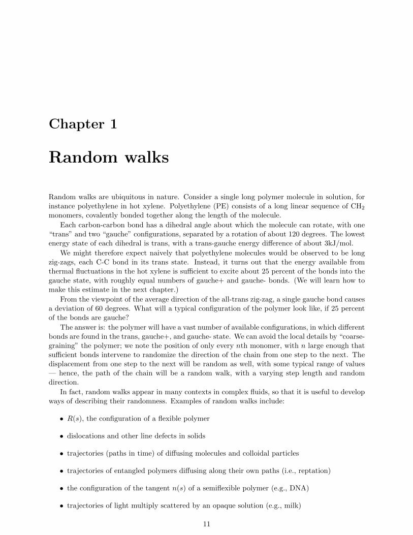
Random walks are ubiquitous in nature. Consider a single long polymer molecule in solution, forinstance polyethylene in hot xylene. Polyethylene (PE) consists of a long linear sequence of CH

2

monomers, covalently bonded together along the length of the molecule.Each carbon-carbon bond has a dihedral angle about which the molecule can rotate, with one

“trans” and two “gauche” configurations, separated by a rotation of about 120 degrees. The lowestenergy state of each dihedral is trans, with a trans-gauche energy di↵erence of about 3kJ/mol.

We might therefore expect naively that polyethylene molecules would be observed to be longzig-zags, each C-C bond in its trans state. Instead, it turns out that the energy available fromthermal fluctuations in the hot xylene is su�cient to excite about 25 percent of the bonds into thegauche state, with roughly equal numbers of gauche+ and gauche- bonds. (We will learn how tomake this estimate in the next chapter.)

From the viewpoint of the average direction of the all-trans zig-zag, a single gauche bond causesa deviation of 60 degrees. What will a typical configuration of the polymer look like, if 25 percentof the bonds are gauche?

The answer is: the polymer will have a vast number of available configurations, in which di↵erentbonds are found in the trans, gauche+, and gauche- state. We can avoid the local details by “coarse-graining” the polymer; we note the position of only every nth monomer, with n large enough thatsu�cient bonds intervene to randomize the direction of the chain from one step to the next. Thedisplacement from one step to the next will be random as well, with some typical range of values— hence, the path of the chain will be a random walk, with a varying step length and randomdirection.

In fact, random walks appear in many contexts in complex fluids, so that it is useful to developways of describing their randomness. Examples of random walks include:

• R(s), the configuration of a flexible polymer

• dislocations and other line defects in solids

• trajectories (paths in time) of di↵using molecules and colloidal particles

• trajectories of entangled polymers di↵using along their own paths (i.e., reptation)

• the configuration of the tangent n(s) of a semiflexible polymer (e.g., DNA)

• trajectories of light multiply scattered by an opaque solution (e.g., milk)

11

12 CHAPTER 1. RANDOM WALKS

In each case, the details — what thing is doing the random walking, and precisely how —are di↵erent. Rather than focus on the details of a particular physical example first (such asthe configurations of polyethylene), we begin with a “toy model” — simple enough to analyze,complicated enough to be interesting. We will then build on our understanding of the toy modelas we consider more physical examples of random walks.

1.1. TOSSING A COIN 13

1.1 Tossing a coin

The simplest example of a random walk is this: toss a coin. If heads, take one step forward; iftails, take one step back. Repeat. Suppose we ask: where will a person playing this game be aftern coin tosses? For a given walker, the answer cannot be known in advance, since it depends on theoutcome of the coin tosses; all we can say is, the walker will be n

+

� n� steps forward, where n+

and n� are the number of heads and tails tossed.

Suppose we assign an entire large lecture class to play this game; we start the game with theclass arranged side by side in a straight line. We can ask, what will be the number of students ssteps from the starting point? (Equivalently, we could assign one student to repeat the game manytimes, and ask how often he ends up s steps ahead.) This question, it turns out, is better posed;although we cannot say in advance where a given walkers will end up, we can predict roughly howmany walkers will end up s steps ahead.

That is, we can predict the probability P (s, n) that a walker will end up s steps ahead after ntosses. The meaning of P (s, n) is: if we repeat the game N times where N is very large, P (s, n) isthe fraction of walks that end up at s.

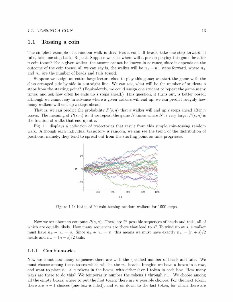
Fig. 1.1 displays a collection of trajectories that result from this simple coin-tossing randomwalk. Although each individual trajectory is random, we can see the trend of the distribution ofpositions; namely, they tend to spread out from the starting point as time progresses.

200 400 600 800 1000

�50

0

50

n

s

Figure 1.1: Paths of 20 coin-tossing random walkers for 1000 steps.

Now we set about to compute P (s, n). There are 2n possible sequences of heads and tails, all ofwhich are equally likely. How many sequences are there that lead to s? To wind up at s, a walkermust have n

+

� n� = s. Since n+

+ n� = n, this means we must have exactly n+

= (n + s)/2heads and n� = (n� s)/2 tails.

1.1.1 Combinatorics

Now we count how many sequences there are with the specified number of heads and tails. Wemust choose among the n tosses which will be the n

+

heads. Imagine we have n boxes in a row,and want to place n

+

< n tokens in the boxes, with either 0 or 1 token in each box. How manyways are there to do this? We temporarily number the tokens 1 through n

+

. We choose amongall the empty boxes, where to put the first token; there are n possible choices. For the next token,there are n � 1 choices (one box is filled), and so on down to the last token, for which there are


n� (n+

� 1) choices. Each of these choices is independent; the total number of arrangements is theproduct, n⇥ (n� 1)⇥ . . . n� (n

+

� 1), which is n!/(n� n+

)!.But the numbers on the tokens were temporary; the tokens were actually identical. From the

above process, for a given selection of boxes filled, the numbers on the tokens will appear once inevery possible order. The number of ways to order the numbered tokens is n

+

! (again, think ofselecting which numbered token will be first, for which there are n

+

choices, which second, and soon down to the last; the choices are independent, and the product is n

+

!.)Every distinct arrangement of the n

+

unnumbered tokens appears n+

! times, one each for everyordering of the temporary numbers on the tokens. Hence the number of distinct ways of choosingn+

places to put a token among n boxes is n!/(n�n+

)!n+

!. This quantity is written�

nn+

�, read “n

choose n+

”, and is called the binomial coe�cient.The probability of any particular sequence of heads and tails being chosen is the same, namely

1/2n (one sequence out of 2n possible). So the probability of a walk that winds up at s is

P (s, n) = 2�n n!

n+

!(n� n+

)!= 2�n

✓n

n+

◆= 2�n

✓n

n�

◆= 2�n n!

(n+ s)/2!(n� s)/2!(1.1)

Note that P (s, n) is an even function of s, i.e., it is symmetric under interchange s ! �s; thusthe probability of ending up s steps ahead equals the probability of ending up s steps behind.

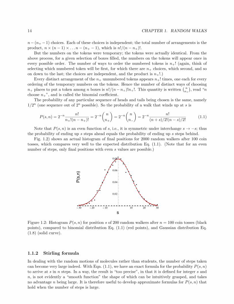
Fig. 1.2) shows an actual histogram of final positions for 2000 random walkers after 100 cointosses, which compares very well to the expected distribution Eq. (1.1). (Note that for an evennumber of steps, only final positions with even s values are possible.)

�30 �20 �10 10 20 30

0.02

0.04

0.06

0.08

s

P(s,n)

Figure 1.2: Histogram P (s, n) for position s of 200 random walkers after n = 100 coin tosses (blackpoints), compared to binomial distribution Eq. (1.1) (red points), and Gaussian distribution Eq.(1.8) (solid curve).

1.1.2 Stirling formula

In dealing with the random motions of molecules rather than students, the number of steps takencan become very large indeed. With Eqn. (1.1), we have an exact formula for the probability P (s, n)to arrive at s in n steps. In a way, the result is “too precise”, in that it is defined for integer s andn, is not evidently a “smooth function” the shape of which can be intuitively grasped, and takesno advantage n being large. It is therefore useful to develop approximate formulas for P (s, n) thathold when the number of steps is large.

1.1. TOSSING A COIN 15

Because the factorial appears repeatedly in P (s, n), it would be very useful to have a simpleapproximation for n! that takes advantage of n being large. Consider how n! changes when weincrease n by one: we acquire one more factor, of (n+ 1). We would like to construct an approxi-mation to the derivative dn!/dn, which we could then integrate to obtain an approximate formulafor n!.

What turns out to be more convenient is to work with log n!, since the change in log n! on incre-menting n by one is additive, namely � log n! = log(n+ 1). Then we can write an approximationfor the derivative as

d log n!

dn⇡ � log n!

�n= log(n+ 1) ⇡ log n (1.2)

This we can integrate, to obtainlog n! ⇡ n log n� n (1.3)

More precise methods yield Stirling’s formula,

n! =p2⇡n

⇣ne

⌘n(1 +O(1/n)) (1.4)

[In Eq. (1.4), the factor (n/e)n corresponds to the simple approximation for log n! we derived inEq. (1.3).]

We use the simplified Stirling approximation to simplify P (s, n): after a bit of algebra (whichyou should do for yourself), we have

logP (s, n) ⇡ �(n/2) [(1 + s/n) log(1 + s/n) + (1� s/n) log(1� s/n)] (1.5)

Note the symmetry of this function under exchange of s and �s, which makes physical sense foran unbiased random walk, for which it is equally likely to throw n

+

heads and n� tails as to thrown+

tails and n� heads.Now we expect P (s, n) to have a maximum — the most likely outcome — which on symmetry

grounds must be s = 0. We expand about this point (s/n is a convenient expansion variable), tofind the “spread” (variance) in the final locations.

Since P (s, n) is even in s, its first derivative at s = 0 vanishes; we have

logP (s, n) = �n/2⇥(s/n)2 +O(s/n)4

⇤(1.6)

Thus we have an approximately Gaussian probability distribution for s

P (s, n) / e�s2/2n (1.7)

We fix the normalization (which our Stirling approximation has been sloppy about) by requiringthe integral under P (s, n) be unity: this gives

P (s, n) =e�s2/2n

(2⇡n)1/2(1.8)

(In setting the normalization, we used the Gaussian integral result from Appendix B,Z 1

�1dx e�↵x2

= (⇡/↵)1/2

A useful measure of the spread of possible values of s is the variance �2, defined as the averagesquare distance of s values from the average, h(s� hsi)2i. In the present example, the average hsivanishes by symmetry, so we have simply

�2 = hs2i = n (1.9)


That is, there are “square root of n fluctuations” in the position of the walker after n steps.(To compute this, note that we can get the integral of x2 times a Gaussian by di↵erentiating

with respect to ↵ (see Appendix B):Z

dx x2e�↵x2= �@↵

Zdx e�↵x2

= �@↵(⇡/↵)1/2 =

(⇡/↵)1/2

2↵

Then the average we seek is

hx2i =Rdx x2e�↵x2

Rdx e�↵x2 =

1

2↵

In the present case, ↵ is 1/2n, whereupon hs2i = n.)(This integral result motivates us sometimes to write the Gaussian probability distribution as

P (s) =e�s2/2�2

(2⇡�2)1/2(1.10)

in which the variance �2 is a parameter.)If the variance were all we wanted to know about a random process, we can compute it without

going to all the trouble to first compute the distribution function P (s, n). This is a very usefulshortcut if we know beforehand by some argument that the random process gives rise to a randomwalk and therefore a Gaussian distribution. For example, we can write the displacement x for a 1drandom process in which a step of length a is taken in direction ni on the ith step (ni = ±1), as

s = aX

i

ni (1.11)

If the random walk is unbiased, then the {ni} are equally likely to be +1 and �1, so that theaverage hnii = 0, and hence s = 0. The variance hs2i can be computed as

hs2i = a2X

i,j

hninji

= a2

0

@X

i=j

hn2

i i+X

i 6=j

hninji

1

A

= na2 + a2X

i 6=j

hniihnji

= na2 (1.12)

In the above, we 1) write “two copies” of the sum for s to be averaged; 2) separate terms into thosein which the same ni appears twice, and those in which two di↵erent ni appear; 3) observe thatn2

i = 1, and use the fact that di↵erent steps are uncorrelated so that the average over ni and nj inhninji can be carried out separately; 4) recall that hnii vanishes for an unbiased walk.

Note finally that precisely the same sequence of steps works if we instead consider a randomwalk in d = 3 dimensions, in which steps of fixed length a are taken in random directions ni (nowinterpreted as random vectors on the unit sphere). Now the variance hr2i of the vector displacementr = a

Pi ni can be computed just as above (with ninj replaced by ni ·nj), and the same final result,

hr2i = na2.

1.2. CONTINUUM DESCRIPTION 17

1.2 Continuum description

In the previous section, we approximated the discrete binomial distribution for a random walk bya continuous Gaussian distribution. This is convenient, because averages with continuous distribu-tions involve integrals, which are often easier to compute than discrete sums. However, sometimesit is useful to describe a random walk process in continuum language to start with. We can do thatby working out how the distribution function itself evolves as the total number of steps increases.

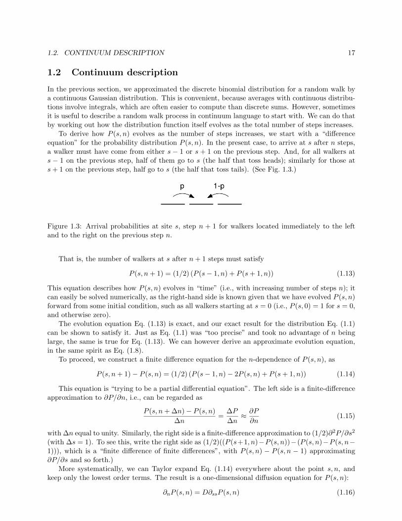
To derive how P (s, n) evolves as the number of steps increases, we start with a “di↵erenceequation” for the probability distribution P (s, n). In the present case, to arrive at s after n steps,a walker must have come from either s � 1 or s + 1 on the previous step. And, for all walkers ats � 1 on the previous step, half of them go to s (the half that toss heads); similarly for those ats+ 1 on the previous step, half go to s (the half that toss tails). (See Fig. 1.3.)

Figure 1.3: Arrival probabilities at site s, step n + 1 for walkers located immediately to the leftand to the right on the previous step n.

That is, the number of walkers at s after n+ 1 steps must satisfy

P (s, n+ 1) = (1/2) (P (s� 1, n) + P (s+ 1, n)) (1.13)

This equation describes how P (s, n) evolves in “time” (i.e., with increasing number of steps n); itcan easily be solved numerically, as the right-hand side is known given that we have evolved P (s, n)forward from some initial condition, such as all walkers starting at s = 0 (i.e., P (s, 0) = 1 for s = 0,and otherwise zero).

The evolution equation Eq. (1.13) is exact, and our exact result for the distribution Eq. (1.1)can be shown to satisfy it. Just as Eq. (1.1) was “too precise” and took no advantage of n beinglarge, the same is true for Eq. (1.13). We can however derive an approximate evolution equation,in the same spirit as Eq. (1.8).

To proceed, we construct a finite di↵erence equation for the n-dependence of P (s, n), as

P (s, n+ 1)� P (s, n) = (1/2) (P (s� 1, n)� 2P (s, n) + P (s+ 1, n)) (1.14)

This equation is “trying to be a partial di↵erential equation”. The left side is a finite-di↵erenceapproximation to @P/@n, i.e., can be regarded as

P (s, n+�n)� P (s, n)

�n=

�P

�n⇡ @P

@n(1.15)

with�n equal to unity. Similarly, the right side is a finite-di↵erence approximation to (1/2)@2P/@s2

(with �s = 1). To see this, write the right side as (1/2)((P (s+1, n)�P (s, n))� (P (s, n)�P (s, n�1))), which is a “finite di↵erence of finite di↵erences”, with P (s, n) � P (s, n � 1) approximating@P/@s and so forth.)

More systematically, we can Taylor expand Eq. (1.14) everywhere about the point s, n, andkeep only the lowest order terms. The result is a one-dimensional di↵usion equation for P (s, n):

@nP (s, n) = D@ssP (s, n) (1.16)


with di↵usion coe�cient D = 1/2. This is a remarkable result: the probability distribution evolvesby di↵usion, according to a deterministic equation. Even though individual particles di↵use ran-domly, the evolution of a cloud of di↵using particles is predictable.

In the above, we have measured time in units of the total number of steps taken n, and distancein units of the number of steps s from the origin. To put physical dimensions back into the problem,we can define time t such that t = n�t where each step takes a time �t, and distance x such thatx = sa where each step forward or back moves the random walker by a length a. Changing variablesfrom n and s to t and x gives

@tP (x, t) = D@xxP (x, t) (1.17)

where now the di↵usion coe�cient is D = a2/(2�t).As more steps are taken (as time passes), the “cloud” of random walkers broadens. By direct

substitution, we can verify that the continuum expression for P (s, n) is a solution to the abovedi↵usion equation. (The equation can also be solved directly by using Fourier transforms.)

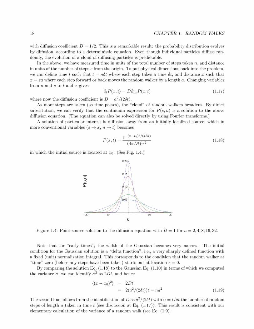
A solution of particular interest is di↵usion away from an initially localized source, which inmore conventional variables (s ! x, n ! t) becomes

P (x, t) =e�(x�x0)

2/(4Dt)

(4⇡Dt)1/2(1.18)

in which the initial source is located at x0

. (See Fig. 1.4.)

�20 �10 10 20

0.05

0.10

0.15

0.20

s

P(s,n)

Figure 1.4: Point-source solution to the di↵usion equation with D = 1 for n = 2, 4, 8, 16, 32.

Note that for “early times”, the width of the Gaussian becomes very narrow. The initialcondition for the Gaussian solution is a “delta function”, i.e., a very sharply defined function witha fixed (unit) normalization integral. This corresponds to the condition that the random walker at“time” zero (before any steps have been taken) starts out at location s = 0.

By comparing the solution Eq. (1.18) to the Gaussian Eq. (1.10) in terms of which we computedthe variance �, we can identify �2 as 2Dt, and hence

h(x� x0

)2i = 2Dt

= 2(a2/(2�t))t = na2 (1.19)

The second line follows from the identification of D as a2/(2�t) with n = t/�t the number of randomsteps of length a taken in time t (see discussion at Eq. (1.17)). This result is consistent with ourelementary calculation of the variance of a random walk (see Eq. (1.9).


In multiple space dimensions, the di↵usion equation takes the form

@tP (r, t) = Dr2P (r, t) (1.20)

with point-source solution

P (r, t) =e�(r�r0)2/(4Dt)

(4⇡Dt)3/2(1.21)

which can be verified by explicit substitution into Eq. (1.20).This 3d point-source solution is just a product of three 1d point-source solutions, since (r�r

0

)2 =(x� x

0

)2 + (y � y0

)2 + (z � z0

)2 and so we have

e�(r�r0)2/(4Dt) = e�(x�x0)2/(4Dt)e�(y�y0)2/(4Dt)e�(z�z0)2/(4Dt) (1.22)

One can e↵ectively regard the random walker as di↵using away from the initial point {x0

, y0

, z0

}independently in the x, y, and z directions.

From this observation it can be seen that the variance h(r � r0

)2i can be written as a sum ofthe variances in each direction, which are all equal:

h(r � r0

)2i = h(x� x0

)2i+ h(y � y0

)2i+ h(z � z0

)2i = 6Dt (1.23)

To make this result correspond to a particular microscopic random walk process, we need onlyadjust the value of D to give the correct variance. For example, if we have an underlying model ofa random walker taking a step of fixed length a every timestep �t in a random direction in d = 3dimensions, we can use Eq. 1.12) to identify D = a2/(6�t).

1.2.1 Conservation law

In multiple space dimensions, the transport equation Eq. (1.16) for P can be written as a conser-vation law,

0 =@P

@t+r · J

J = �DrP (1.24)

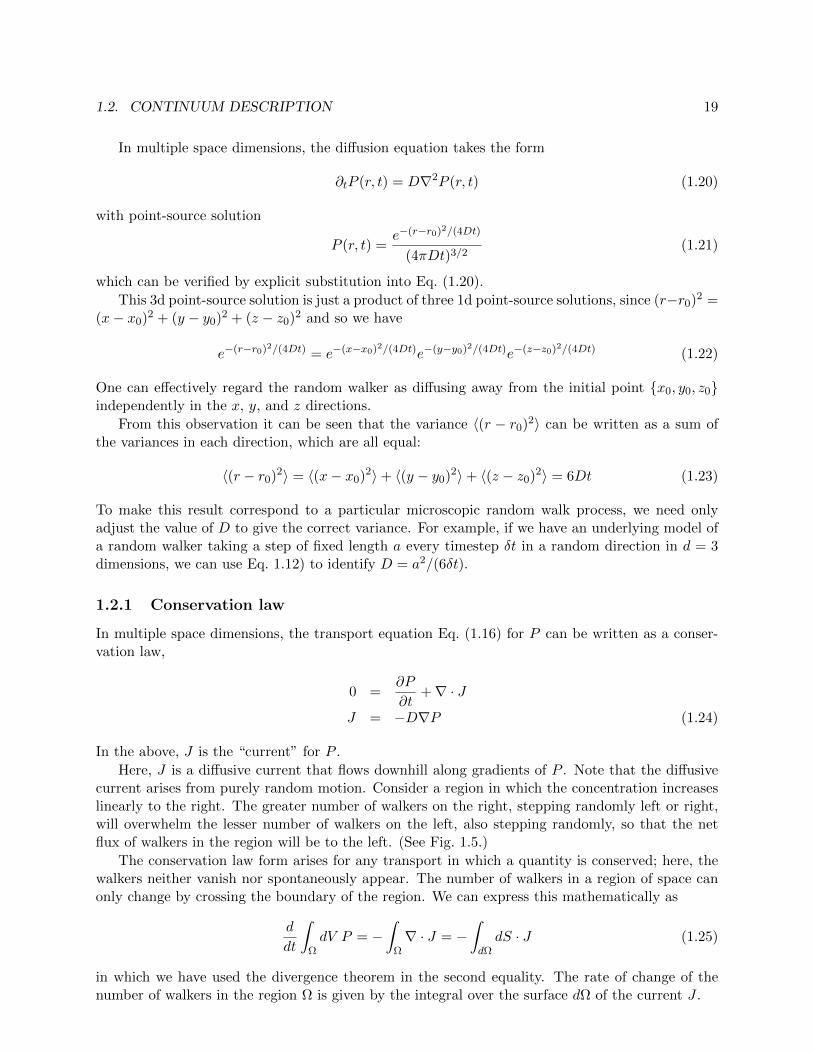
In the above, J is the “current” for P .Here, J is a di↵usive current that flows downhill along gradients of P . Note that the di↵usive

current arises from purely random motion. Consider a region in which the concentration increaseslinearly to the right. The greater number of walkers on the right, stepping randomly left or right,will overwhelm the lesser number of walkers on the left, also stepping randomly, so that the netflux of walkers in the region will be to the left. (See Fig. 1.5.)

The conservation law form arises for any transport in which a quantity is conserved; here, thewalkers neither vanish nor spontaneously appear. The number of walkers in a region of space canonly change by crossing the boundary of the region. We can express this mathematically as

d

dt

Z

⌦

dV P = �Z

⌦

r · J = �Z

d⌦dS · J (1.25)

in which we have used the divergence theorem in the second equality. The rate of change of thenumber of walkers in the region ⌦ is given by the integral over the surface d⌦ of the current J .


Figure 1.5: Greater numbers of walkers to the right, all moving randomly left and right, leads to anet current of walkers to the left.

1.2.2 Biased random walk

Now suppose the coin toss is biased — the coin is weighted, or some other unspecified chicanerytranspires, such that the chance of a head being tossed is p > 1/2. How will P (s, n) change?

The number of walks that arrive at s is unchanged; it still corresponds to the number of walkswith n

+

heads and n� tails such that n+

� n� = s. However, the probability of any particularsequence of heads and tails changes. The probability of any one sequence with n

+

heads and n�tails is pn+(1� p)n� ; hence

P (s, n) = pn++

pn��

n!

n+

!n�!⌘ p(n+s)/2(1� p)(n�s)/2

✓n

(n+ s)/2

◆(1.26)

in which we observe the expected symmetry under interchange of n+

and n� (with p+

interchangedwith p�).

The probability distribution P (s, n) is no longer an even function of s; indeed, we expect thatthe walkers will tend to drift forward at a steady rate of p

+

� p� or 2p� 1 steps per coin toss.Applying the simplified Stirling formula to the above biased random walk result, we find

logP (s, n) ⇡ �(n/2)

(1 + s/n) log

(1 + s/n)

2p+ (1� s/n) log

(1� s/n)

2(1� p)

�(1.27)

To verify that the most-probable value of s (maximum of logP ) is s = (2p�1)n, we set @s logP (s, n)to zero, to find

0 = log(1 + s/n)

2p� log

(1� s/n)

2(1� p)(1.28)

which after a bit of algebra gives the expected result.Now we expand about the maximum to second order as before. After some algebra we find

logP (s, n) ⇡ const +(s� s̄)2

8p(1� p)n(1.29)

in which s̄ = (2p� 1)n.After imposing normalization, we have

P (s, n) =e�(s�s̄)2/(8p(1�p)n)

(8⇡p(1� p)n)1/2(1.30)


�20 �10 10 20 30

0.05

0.10

0.15

0.20

s

P(s,n)

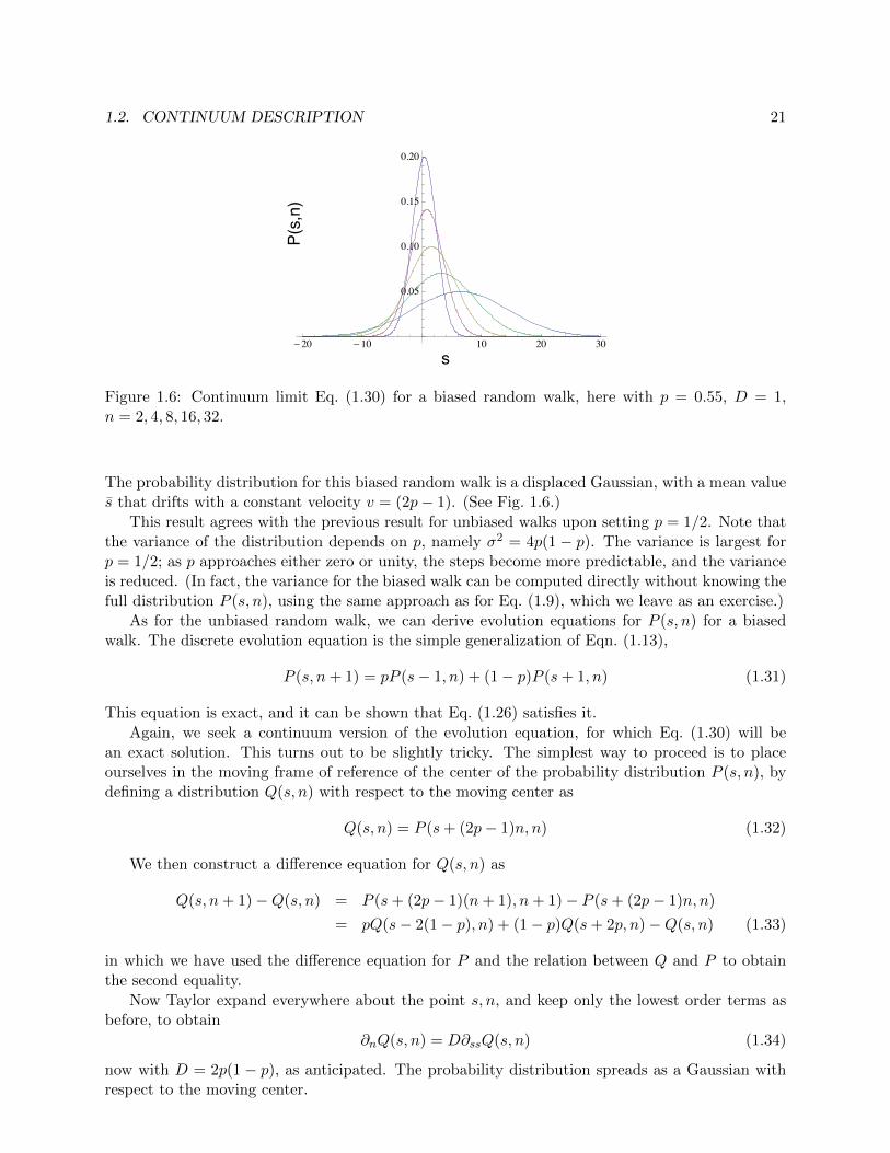
Figure 1.6: Continuum limit Eq. (1.30) for a biased random walk, here with p = 0.55, D = 1,n = 2, 4, 8, 16, 32.

The probability distribution for this biased random walk is a displaced Gaussian, with a mean values̄ that drifts with a constant velocity v = (2p� 1). (See Fig. 1.6.)

This result agrees with the previous result for unbiased walks upon setting p = 1/2. Note thatthe variance of the distribution depends on p, namely �2 = 4p(1 � p). The variance is largest forp = 1/2; as p approaches either zero or unity, the steps become more predictable, and the varianceis reduced. (In fact, the variance for the biased walk can be computed directly without knowing thefull distribution P (s, n), using the same approach as for Eq. (1.9), which we leave as an exercise.)

As for the unbiased random walk, we can derive evolution equations for P (s, n) for a biasedwalk. The discrete evolution equation is the simple generalization of Eqn. (1.13),

P (s, n+ 1) = pP (s� 1, n) + (1� p)P (s+ 1, n) (1.31)

This equation is exact, and it can be shown that Eq. (1.26) satisfies it.Again, we seek a continuum version of the evolution equation, for which Eq. (1.30) will be

an exact solution. This turns out to be slightly tricky. The simplest way to proceed is to placeourselves in the moving frame of reference of the center of the probability distribution P (s, n), bydefining a distribution Q(s, n) with respect to the moving center as

Q(s, n) = P (s+ (2p� 1)n, n) (1.32)

We then construct a di↵erence equation for Q(s, n) as

Q(s, n+ 1)�Q(s, n) = P (s+ (2p� 1)(n+ 1), n+ 1)� P (s+ (2p� 1)n, n)

= pQ(s� 2(1� p), n) + (1� p)Q(s+ 2p, n)�Q(s, n) (1.33)

in which we have used the di↵erence equation for P and the relation between Q and P to obtainthe second equality.

Now Taylor expand everywhere about the point s, n, and keep only the lowest order terms asbefore, to obtain

@nQ(s, n) = D@ssQ(s, n) (1.34)

now with D = 2p(1 � p), as anticipated. The probability distribution spreads as a Gaussian withrespect to the moving center.


Written back in terms of P (s, n), we have a biased di↵usion equation, which again can bewritten as a conservation law:

0 = @nP + @sJ

J = �D@sP + vP (1.35)

in which the current J is the sum of di↵usive and drift contributions, with di↵usion constantD = 2p(1� p) and drift velocity v = (2p� 1).

1.3. CENTRAL LIMIT THEOREM 23

1.3 Central limit theorem

Usually, the elementary steps in a random walk are more complicated than simply one step forwardor one step back with equal likelihood. For example, there may be a range of possible elementarysteps r, each taken with some probability p(r). What can we say about the resulting probabilitydistribution P (s, n) for these more general random walks?

It turns out that under rather general conditions, the distribution after many steps of a randomwalk is still approximately Gaussian, of the form

P (s, n) =e�(s�nhri)2/2nh�r2i

(2⇡nh�r2i)1/2(1.36)

In the above, hri is the average elementary step (zero for an unbiased walk), and h�ri is the averagevariance in the elementary step (�r = r � hri).

This result, called the central limit theorem, holds whenever the elementary step distributionp(r) has finite “moments” (averages of rk for all positive k). It is the reason for the ubiquity ofthe “bell curve” (Gaussian), that the sum of uncorrelated random numbers (here, the steps) has adistribution that becomes Gaussian as the number of summands becomes large.

1.3.1 Proof

Let {ri} be n identical random variables, with probability distribution w(r). We seek the probabilitydistribution P (s) of the sum s =

Pi ri. Evidently the average hsi equals nhri. For convenience,

we shift the definitions of s and the {ri} by subtracting the average values from each, so thathsi = hrii = 0.

We may write formally

P (s) =

Zdr

1

. . . drnw(r1) . . . w(rn)�(s�X

i

ri) (1.37)

It turns out to be useful to take the Fourier transform of both sides. Defining P (q) =Rds e�iqsP (s)

(in probability theory P (q) is called the “characteristic function” for s), we have after a bit of algebra

P (q) = [w(q)]n (1.38)

Now we work out the expansion of w(q) for small q (which, it turns out, is all that we need toknow):

w(q) =

Zdr e�iqrw(r) =

Zdr (1� iqr � q2r2/2 + . . .)w(r)

= 1� (q2/2)hr2i+O(q3hr3i) (1.39)

in which the second term vanished because hri = 0.Now we may write

P (q) =⇥1� (q2/2)hr2i+O(q3hr3i)

⇤n(1.40)

We would like to take the limit of large n, which we can do if we redefine q2 = q02/n, and regardP for the moment as a function of q0: then we have

P (q) =h1� (q02/2n)hr2i(1 +O(n�1/2)

in

! e�(q02/2)hr2i = e�q2nhr2i/2 (1.41)


in which we have at the last returned to writing P as a function of q. (The limit above makes useof the result from calculus limn!1(1 + x/n)n ! ex.)

Now we may invert the Fourier transform, using P (s) =R dq

2⇡eiqsP (q). Performing the Gaussian

integral that results, taking care to fix up the normalization for P (s), and restoring the nonzeroaverage value for s, we have finally

P (s) =e�(s�nhri)2/2nh�r2i

(2⇡nh�r2i)1/2(1.42)

1.4. BOLTZMANN FACTORS 25

1.4 Boltzmann factors

In our discussion of random walks in the previous section, we focused on idealized models in whichindividual steps are governed by the toss of a coin. In physical systems, such as the configurationsof a long polymer chain in a melt or solution, individual steps in a random walk are governed bythe flexibility of the molecule, and the energetic cost to adopt di↵erent local conformations.

As a simple example, consider a long alkane molecule, such as a polyethylene (PE) chain. Thedihedral angles between each successive pair of CH

2

groups can be rotated with a modest energycost; as a result, the chain can adopt many conformations at finite temperature. The shortesthydrocarbon chain with this conformational freedom is butane, which has one such dihedral anglebetween the second and third carbons. At zero temperature, the chain adopts the lowest energystate, in which all bonds are in the trans state, resulting in a planar zig-zag conformation. At highertemperatures, the dihedral angles can take on di↵erent values. What governs the probabilities withwhich these states are found?

It turns out that the probabilities of the available states of a system at a given temperature Tare given by the Boltzmann factor:

Pr / e��Er (1.43)

Here r denotes the “microstate”, or configuration of the degrees of freedom of the problem, Er thecorresponding energy of that state, and � is 1/(kT ), where k is the Boltzmann constant. EvidentlykT has units of energy (so that the exponent is dimensionless). Roughly speaking, kT is the amountof energy typically available to a single degree of freedom for thermal fluctuations at a temperatureT .

Because the system must be in some state or other, the probabilities Pr must sum to unity,which fixes the normalization:

Pr =e��E

r

Z(1.44)

Here Z is the partition function,

Z =X

r

e��Er (1.45)

so called because its summands describe how probability is partitioned among the di↵erent possiblemicrostates. The partition function Z is a function first and foremost of temperature through� = 1/(kT ), which a↵ects the partitioning of probability.

The results Eq. (1.44) and (1.45) are central to statistical mechanics: they predict the probabilityof any state — any arrangement of molecules — of any system in equilibrium. We present thisresult in advance of any proof of its validity, to give a glimpse of where we are heading in the nextchapter, where this result is derived and exploited. For now, we apply this result to the simpleexample of dihedral angles in alkanes, to develop some physical insight into how Boltzmann factorsgovern probabilities as a function of temperature.

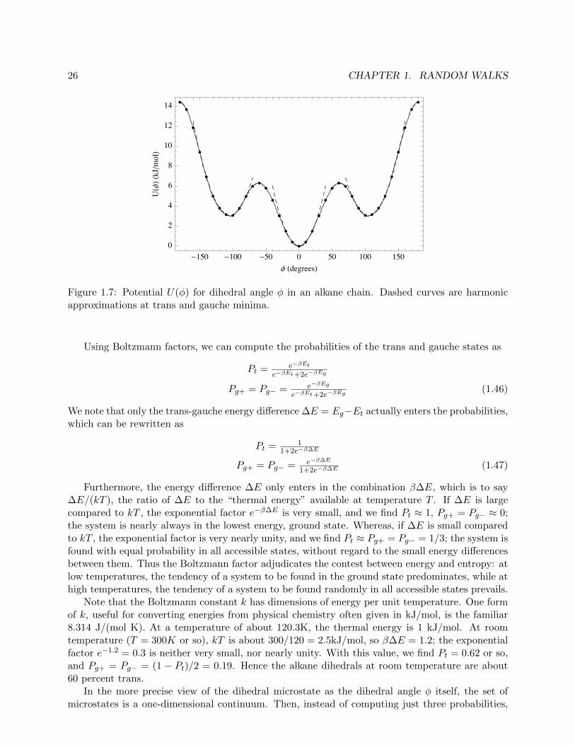
To compute the probabilities for a given system, we must describe its microstates and providethe corresponding energies. The choice of microstates is an opportunity for approximation. Forbutane with its single dihedral angle, the most straightforward choice would be to take the angle� itself as the microstate. The dihedral potential U(�), displayed in Fig. 1.7, would supply thecorresponding energies.

However, we note that U(�) has three well-defined minima, at angles of roughly � = 0 (trans),� = 2⇡/3 (gauche+), and � = 2⇡/3) (gauche-). The energies of the gauche+ and gauche- stateslie about 3kJ/mol above the trans minimum. The three well-defined minima in the potential U(�)suggest a simple approximate set of microstates; namely, a set of three states {t, g+, g�} withenergies Et, Eg (same energy for g+ and g�).


-150 -100 -50 0 50 100 1500

2

4

6

8

10

12

14

f HdegreesL

UHfLH

kJêmo

lL

Figure 1.7: Potential U(�) for dihedral angle � in an alkane chain. Dashed curves are harmonicapproximations at trans and gauche minima.

Using Boltzmann factors, we can compute the probabilities of the trans and gauche states as

Pt =e��E

t

e��E

t

+2e��E

g

Pg+ = Pg� = e��E

g

e��E

t

+2e��E

g

(1.46)

We note that only the trans-gauche energy di↵erence�E = Eg�Et actually enters the probabilities,which can be rewritten as

Pt =1

1+2e��E

Pg+ = Pg� = e��E

1+2e��E

(1.47)

Furthermore, the energy di↵erence �E only enters in the combination ��E, which is to say�E/(kT ), the ratio of �E to the “thermal energy” available at temperature T . If �E is largecompared to kT , the exponential factor e��E is very small, and we find Pt ⇡ 1, Pg+ = Pg� ⇡ 0;the system is nearly always in the lowest energy, ground state. Whereas, if �E is small comparedto kT , the exponential factor is very nearly unity, and we find Pt ⇡ Pg+ = Pg� = 1/3; the system isfound with equal probability in all accessible states, without regard to the small energy di↵erencesbetween them. Thus the Boltzmann factor adjudicates the contest between energy and entropy: atlow temperatures, the tendency of a system to be found in the ground state predominates, while athigh temperatures, the tendency of a system to be found randomly in all accessible states prevails.

Note that the Boltzmann constant k has dimensions of energy per unit temperature. One formof k, useful for converting energies from physical chemistry often given in kJ/mol, is the familiar8.314 J/(mol K). At a temperature of about 120.3K, the thermal energy is 1 kJ/mol. At roomtemperature (T = 300K or so), kT is about 300/120 = 2.5kJ/mol, so ��E = 1.2; the exponentialfactor e�1.2 = 0.3 is neither very small, nor nearly unity. With this value, we find Pt = 0.62 or so,and Pg+ = Pg� = (1 � Pt)/2 = 0.19. Hence the alkane dihedrals at room temperature are about60 percent trans.

In the more precise view of the dihedral microstate as the dihedral angle � itself, the set ofmicrostates is a one-dimensional continuum. Then, instead of computing just three probabilities,

1.4. BOLTZMANN FACTORS 27

we determine the probability distribution P (�), again from the general expression Eq. (1.44), inwhich the “sum” over microstates

Pr becomes an integral over �.

The probability of the dihedral angle being within d� of given value � is given by P (�)d�, whereP (�) is the probability distribution, written as

P (�) =e��U(�)

Z(1.48)

with the partition function given by

Z =

Z2⇡

0

d� e��U(�) (1.49)

This expression looks a bit di↵erent from the general result Eq. (1.44) and (1.45), but funda-mentally it is the same: � is the microstate r, the integral

R2⇡0

d� is the sumP

r over microstates,

and e��U(�) is the Boltzmann factor e��Er . The probability P (�) is properly normalized by the

denominator Z =R2⇡0

d�P (�) gives unity, as the denominator is designed to cancel the integral ofthe numerator.

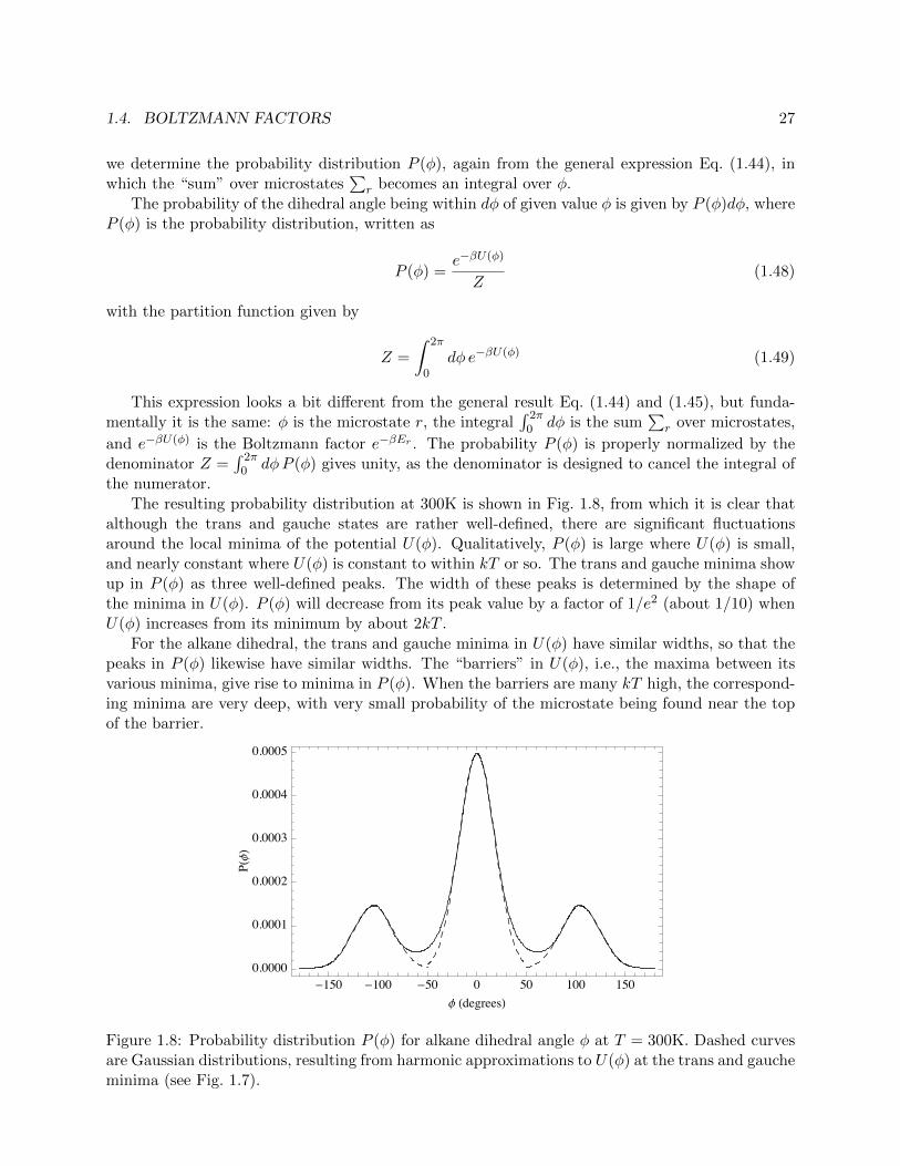
The resulting probability distribution at 300K is shown in Fig. 1.8, from which it is clear thatalthough the trans and gauche states are rather well-defined, there are significant fluctuationsaround the local minima of the potential U(�). Qualitatively, P (�) is large where U(�) is small,and nearly constant where U(�) is constant to within kT or so. The trans and gauche minima showup in P (�) as three well-defined peaks. The width of these peaks is determined by the shape ofthe minima in U(�). P (�) will decrease from its peak value by a factor of 1/e2 (about 1/10) whenU(�) increases from its minimum by about 2kT .

For the alkane dihedral, the trans and gauche minima in U(�) have similar widths, so that thepeaks in P (�) likewise have similar widths. The “barriers” in U(�), i.e., the maxima between itsvarious minima, give rise to minima in P (�). When the barriers are many kT high, the correspond-ing minima are very deep, with very small probability of the microstate being found near the topof the barrier.

-150 -100 -50 0 50 100 1500.0000

0.0001

0.0002

0.0003

0.0004

0.0005

f HdegreesL

PHfL

Figure 1.8: Probability distribution P (�) for alkane dihedral angle � at T = 300K. Dashed curvesare Gaussian distributions, resulting from harmonic approximations to U(�) at the trans and gaucheminima (see Fig. 1.7).


We can construct a good representation for these fluctuations about the trans and gaucheminima by expanding the potential U(�) to quadratic order around the minimum � values. Thisleads to a Gaussian approximation for P (�) in the vicinity of the minima of U(�), as

U(�) ⇡ U(�⇤) + (1/2)U 00(�⇤)(�� ⇤)2

P (�) / e�U(�⇤)+(1/2)U 00

(�⇤)(��⇤

)

2(1.50)

The resulting harmonic approximate potentials are shown as dashed curves in Fig. 1.7; the cor-responding Gaussian approximate distributions resulting from Eqn. (1.50) are shown as dashedcurves in Fig. 1.8.

The reason the harmonic approximation works so well here, is that the dihedral potential iswell described by a quadratic for several kJ/mol above the minima. The typical scale of energyfluctuations for a single degree of freedom is kT , which at 300K is about 2.5kJ/mol. So if thepotential is reasonably quadratic as far as 5kJ from the minimum, only relatively rare fluctuationswill reach dihedral angles at which the potential is “anharmonic” (i.e., not quadratic), and thecorresponding probability distribution will be very nearly Gaussian.

Given the continuous probability distribution P (�), we could define what it means to be in thetrans, gauche+, or gauche- states by partitioning the range of � into regions, perhaps between theminima of P (�). We could then integrate (numerically) P (�) in these regions to compute Pt andPg± (which, because P (�) is properly normalized, would sum to unity). In such integrals, it is clearthat the width as well as the height of the peaks in P (�) matter in determining Pt and Pg±.

Indeed, we could roughly approximate Pt as the peak height times the width — the largesttypical probability of the set of microstates near the trans minimum, times the number of stateswithin kT or so of the minimum. A deep but narrow minimum would have very favorable energy(a tall peak), but few nearby states; a shallow by wide minimum would have a shorter but broaderpeak. The probabilities of being found near two distinct minima 1 and 2 will be about equal when

N1

exp(��E1

) ⇡ N2

exp(��E2

) (1.51)

where N1

and N2

are the number of microstates (range of � values, in our dihedral example) withinkT or so of the corresponding minima.

Taking the log and multiplying by kT , this can be rearranged to

E1

� kT logN1

= E2

� kT logN2

(1.52)

This result is very reminiscent of the thermodynamic relation between two phases in equilibrium,for which (neglecting contributions from volume changes) the Helmholtz free energies F = E� TSare equal. This foreshadows the statistical definition of the entropy S as S = k logN , where N isthe number of accessible states, which we shall explore in detail in the next chapter.

Documents

Random walks - Pennsylvania State University