Random Walks - Dartmouth Collegechance/teaching_aids/books... · Random Walks 12.1 Random Walks in ... The sequence fS ng1n =1 is called a random walk. ... say, after nmoves, with

Chapter 12

Random Walks

12.1 Random Walks in Euclidean Space

In the last several chapters, we have studied sums of random variables with the goalbeing to describe the distribution and density functions of the sum. In this chapter,we shall look at sums of discrete random variables from a different perspective. Weshall be concerned with properties which can be associated with the sequence ofpartial sums, such as the number of sign changes of this sequence, the number ofterms in the sequence which equal 0, and the expected size of the maximum termin the sequence.

We begin with the following definition.

Definition 12.1 Let {Xk}∞k=1 be a sequence of independent, identically distributeddiscrete random variables. For each positive integer n, we let Sn denote the sumX1 +X2 + · · ·+Xn. The sequence {Sn}∞n=1 is called a random walk. If the commonrange of the Xk’s is Rm, then we say that {Sn} is a random walk in Rm. 2

We view the sequence of Xk’s as being the outcomes of independent experiments.Since the Xk’s are independent, the probability of any particular (finite) sequenceof outcomes can be obtained by multiplying the probabilities that each Xk takeson the specified value in the sequence. Of course, these individual probabilities aregiven by the common distribution of the Xk’s. We will typically be interested infinding probabilities for events involving the related sequence of Sn’s. Such eventscan be described in terms of the Xk’s, so their probabilities can be calculated usingthe above idea.

There are several ways to visualize a random walk. One can imagine that aparticle is placed at the origin in Rm at time n = 0. The sum Sn represents theposition of the particle at the end of n seconds. Thus, in the time interval [n−1, n],the particle moves (or jumps) from position Sn−1 to Sn. The vector representingthis motion is just Sn−Sn−1, which equals Xn. This means that in a random walk,the jumps are independent and identically distributed. If m = 1, for example, thenone can imagine a particle on the real line that starts at the origin, and at theend of each second, jumps one unit to the right or the left, with probabilities given

471

472 CHAPTER 12. RANDOM WALKS

by the distribution of the Xk’s. If m = 2, one can visualize the process as takingplace in a city in which the streets form square city blocks. A person starts at onecorner (i.e., at an intersection of two streets) and goes in one of the four possibledirections according to the distribution of the Xk’s. If m = 3, one might imaginebeing in a jungle gym, where one is free to move in any one of six directions (left,right, forward, backward, up, and down). Once again, the probabilities of thesemovements are given by the distribution of the Xk’s.

Another model of a random walk (used mostly in the case where the range isR1) is a game, involving two people, which consists of a sequence of independent,identically distributed moves. The sum Sn represents the score of the first person,say, after n moves, with the assumption that the score of the second person is−Sn. For example, two people might be flipping coins, with a match or non-matchrepresenting +1 or −1, respectively, for the first player. Or, perhaps one coin isbeing flipped, with a head or tail representing +1 or −1, respectively, for the firstplayer.

Random Walks on the Real Line

We shall first consider the simplest non-trivial case of a random walk in R1, namelythe case where the common distribution function of the random variables Xn isgiven by

fX(x) ={

1/2, if x = ±1,0, otherwise.

This situation corresponds to a fair coin being flipped, with Sn representing thenumber of heads minus the number of tails which occur in the first n flips. We notethat in this situation, all paths of length n have the same probability, namely 2−n.

It is sometimes instructive to represent a random walk as a polygonal line, orpath, in the plane, where the horizontal axis represents time and the vertical axisrepresents the value of Sn. Given a sequence {Sn} of partial sums, we first plot thepoints (n, Sn), and then for each k < n, we connect (k, Sk) and (k+ 1, Sk+1) with astraight line segment. The length of a path is just the difference in the time valuesof the beginning and ending points on the path. The reader is referred to Figure12.1. This figure, and the process it illustrates, are identical with the example,given in Chapter 1, of two people playing heads or tails.

Returns and First Returns

We say that an equalization has occurred, or there is a return to the origin at timen, if Sn = 0. We note that this can only occur if n is an even integer. To calculatethe probability of an equalization at time 2m, we need only count the number ofpaths of length 2m which begin and end at the origin. The number of such pathsis clearly (

2mm

).

Since each path has probability 2−2m, we have the following theorem.

12.1. RANDOM WALKS IN EUCLIDEAN SPACE 473

5 10 15 20 25 30 35 40

-10

-8

-6

-4

-2

2

4

6

8

10

Figure 12.1: A random walk of length 40.

Theorem 12.1 The probability of a return to the origin at time 2m is given by

u2m =(

2mm

)2−2m .

The probability of a return to the origin at an odd time is 0. 2

A random walk is said to have a first return to the origin at time 2m if m > 0, andS2k 6= 0 for all k < m. In Figure 12.1, the first return occurs at time 2. We definef2m to be the probability of this event. (We also define f0 = 0.) One can thinkof the expression f2m22m as the number of paths of length 2m between the points(0, 0) and (2m, 0) that do not touch the horizontal axis except at the endpoints.Using this idea, it is easy to prove the following theorem.

Theorem 12.2 For n ≥ 1, the probabilities {u2k} and {f2k} are related by theequation

u2n = f0u2n + f2u2n−2 + · · ·+ f2nu0 .

Proof. There are u2n22n paths of length 2n which have endpoints (0, 0) and (2n, 0).The collection of such paths can be partitioned into n sets, depending upon the timeof the first return to the origin. A path in this collection which has a first return tothe origin at time 2k consists of an initial segment from (0, 0) to (2k, 0), in whichno interior points are on the horizontal axis, and a terminal segment from (2k, 0)to (2n, 0), with no further restrictions on this segment. Thus, the number of pathsin the collection which have a first return to the origin at time 2k is given by

f2k22ku2n−2k22n−2k = f2ku2n−2k22n .

If we sum over k, we obtain the equation

u2n22n = f0u2n22n + f2u2n−222n + · · ·+ f2nu022n .

Dividing both sides of this equation by 22n completes the proof. 2


The expression in the right-hand side of the above theorem should remind the readerof a sum that appeared in Definition 7.1 of the convolution of two distributions. Theconvolution of two sequences is defined in a similar manner. The above theoremsays that the sequence {u2n} is the convolution of itself and the sequence {f2n}.Thus, if we represent each of these sequences by an ordinary generating function,then we can use the above relationship to determine the value f2n.

Theorem 12.3 For m ≥ 1, the probability of a first return to the origin at time2m is given by

f2m =u2m

2m− 1=

(2mm

)(2m− 1)22m

.

Proof. We begin by defining the generating functions

U(x) =∞∑m=0

u2mxm

and

F (x) =∞∑m=0

f2mxm .

Theorem 12.2 says thatU(x) = 1 + U(x)F (x) . (12.1)

(The presence of the 1 on the right-hand side is due to the fact that u0 is definedto be 1, but Theorem 12.2 only holds for m ≥ 1.) We note that both generatingfunctions certainly converge on the interval (−1, 1), since all of the coefficients are atmost 1 in absolute value. Thus, we can solve the above equation for F (x), obtaining

F (x) =U(x)− 1U(x)

.

Now, if we can find a closed-form expression for the function U(x), we will also havea closed-form expression for F (x). From Theorem 12.1, we have

U(x) =∞∑m=0

(2mm

)2−2mxm .

In Wilf,1 we find that1√

1− 4x=∞∑m=0

(2mm

)xm .

The reader is asked to prove this statement in Exercise 1. If we replace x by x/4in the last equation, we see that

U(x) =1√

1− x.

1H. S. Wilf, Generatingfunctionology, (Boston: Academic Press, 1990), p. 50.


Therefore, we have

F (x) =U(x)− 1U(x)

=(1− x)−1/2 − 1

(1− x)−1/2

= 1− (1− x)1/2 .

Although it is possible to compute the value of f2m using the Binomial Theorem,it is easier to note that F ′(x) = U(x)/2, so that the coefficients f2m can be foundby integrating the series for U(x). We obtain, for m ≥ 1,

f2m =u2m−2

2m

=

(2m−2m−1

)m22m−1

=

(2mm

)(2m− 1)22m

=u2m

2m− 1,

since (2m− 2m− 1

)=

m

2(2m− 1)

(2mm

).

This completes the proof of the theorem. 2

Probability of Eventual Return

In the symmetric random walk process in Rm, what is the probability that theparticle eventually returns to the origin? We first examine this question in the casethat m = 1, and then we consider the general case. The results in the next twoexamples are due to Polya.2

Example 12.1 (Eventual Return in R1) One has to approach the idea of eventualreturn with some care, since the sample space seems to be the set of all walks ofinfinite length, and this set is non-denumerable. To avoid difficulties, we will definewn to be the probability that a first return has occurred no later than time n. Thus,wn concerns the sample space of all walks of length n, which is a finite set. In termsof the wn’s, it is reasonable to define the probability that the particle eventuallyreturns to the origin to be

w∗ = limn→∞

wn .

This limit clearly exists and is at most one, since the sequence {wn}∞n=1 is anincreasing sequence, and all of its terms are at most one.

2G. Polya, “Uber eine Aufgabe der Wahrscheinlichkeitsrechnung betreffend die Irrfahrt imStrassennetz,” Math. Ann., vol. 84 (1921), pp. 149-160.


In terms of the fn probabilities, we see that

w2n =n∑i=1

f2i .

Thus,

w∗ =∞∑i=1

f2i .

In the proof of Theorem 12.3, the generating function

F (x) =∞∑m=0

f2mxm

was introduced. There it was noted that this series converges for x ∈ (−1, 1). Infact, it is possible to show that this series also converges for x = ±1 by usingExercise 4, together with the fact that

f2m =u2m

2m− 1.

(This fact was proved in the proof of Theorem 12.3.) Since we also know that

F (x) = 1− (1− x)1/2 ,

we see thatw∗ = F (1) = 1 .

Thus, with probability one, the particle returns to the origin.An alternative proof of the fact that w∗ = 1 can be obtained by using the results

in Exercise 2. 2

Example 12.2 (Eventual Return in Rm) We now turn our attention to the casethat the random walk takes place in more than one dimension. We define f (m)

2n tobe the probability that the first return to the origin in Rm occurs at time 2n. Thequantity u(m)

2n is defined in a similar manner. Thus, f (1)2n and u(1)

2n equal f2n and u2n,which were defined earlier. If, in addition, we define u(m)

0 = 1 and f(m)0 = 0, then

one can mimic the proof of Theorem 12.2, and show that for all m ≥ 1,

u(m)2n = f

(m)0 u

(m)2n + f

(m)2 u

(m)2n−2 + · · ·+ f

(m)2n u

(m)0 . (12.2)

We continue to generalize previous work by defining

U (m)(x) =∞∑n=0

u(m)2n xn

and

F (m)(x) =∞∑n=0

f(m)2n xn .


Then, by using Equation 12.2, we see that

U (m)(x) = 1 + U (m)(x)F (m)(x) ,

as before. These functions will always converge in the interval (−1, 1), since all oftheir coefficients are at most one in magnitude. In fact, since

w(m)∗ =

∞∑n=0

f(m)2n ≤ 1

for all m, the series for F (m)(x) converges at x = 1 as well, and F (m)(x) is left-continuous at x = 1, i.e.,

limx↑1

F (m)(x) = F (m)(1) .

Thus, we have

w(m)∗ = lim

x↑1F (m)(x) = lim

x↑1

U (m)(x)− 1U (m)(x)

, (12.3)

so to determine w(m)∗ , it suffices to determine

limx↑1

U (m)(x) .

We let u(m) denote this limit.We claim that

u(m) =∞∑n=0

u(m)2n .

(This claim is reasonable; it says that to find out what happens to the functionU (m)(x) at x = 1, just let x = 1 in the power series for U (m)(x).) To prove theclaim, we note that the coefficients u(m)

2n are non-negative, so U (m)(x) increasesmonotonically on the interval [0, 1). Thus, for each K, we have

K∑n=0

u(m)2n ≤ lim

x↑1U (m)(x) = u(m) ≤

∞∑n=0

u(m)2n .

By letting K →∞, we see that

u(m) =∞∑2n

u(m)2n .

This establishes the claim.From Equation 12.3, we see that if u(m) <∞, then the probability of an eventual

return isu(m) − 1u(m)

,

while if u(m) =∞, then the probability of eventual return is 1.To complete the example, we must estimate the sum

∞∑n=0

u(m)2n .


In Exercise 12, the reader is asked to show that

u(2)2n =

142n

(2nn

)2

.

Using Stirling’s Formula, it is easy to show that (see Exercise 13)(2nn

)∼ 22n

√πn

,

sou

(2)2n ∼

1πn

.

From this it follows easily that∞∑n=0

u(2)2n

diverges, so w(2)∗ = 1, i.e., in R2, the probability of an eventual return is 1.

When m = 3, Exercise 12 shows that

u(3)2n =

122n

(2nn

)∑j,k

(13n

n!j!k!(n− j − k)!

)2

.

Let M denote the largest value of

n!j!k!(n− j − k)!

,

over all non-negative values of j and k with j + k ≤ n. It is easy, using Stirling’sFormula, to show that

M ∼ c

n,

for some constant c. Thus, we have

u(3)2n ≤

122n

(2nn

)∑j,k

(M

3nn!

j!k!(n− j − k)!

).

Using Exercise 14, one can show that the right-hand expression is at most

c′

n3/2,

where c′ is a constant. Thus,∞∑n=0

u(3)2n

converges, so w(3)∗ is strictly less than one. This means that in R3, the probability of

an eventual return to the origin is strictly less than one (in fact, it is approximately.65).

One may summarize these results by stating that one should not get drunk inmore than two dimensions. 2


Expected Number of Equalizations

We now give another example of the use of generating functions to find a generalformula for terms in a sequence, where the sequence is related by recursion relationsto other sequences. Exercise 9 gives still another example.

Example 12.3 (Expected Number of Equalizations) In this example, we will de-rive a formula for the expected number of equalizations in a random walk of length2m. As in the proof of Theorem 12.3, the method has four main parts. First, arecursion is found which relates the mth term in the unknown sequence to earlierterms in the same sequence and to terms in other (known) sequences. An exam-ple of such a recursion is given in Theorem 12.2. Second, the recursion is usedto derive a functional equation involving the generating functions of the unknownsequence and one or more known sequences. Equation 12.1 is an example of sucha functional equation. Third, the functional equation is solved for the unknowngenerating function. Last, using a device such as the Binomial Theorem, integra-tion, or differentiation, a formula for the mth coefficient of the unknown generatingfunction is found.

We begin by defining g2m to be the number of equalizations among all of therandom walks of length 2m. (For each random walk, we disregard the equalizationat time 0.) We define g0 = 0. Since the number of walks of length 2m equals 22m,the expected number of equalizations among all such random walks is g2m/22m.Next, we define the generating function G(x):

G(x) =∞∑k=0

g2kxk .

Now we need to find a recursion which relates the sequence {g2k} to one or both ofthe known sequences {f2k} and {u2k}. We consider m to be a fixed positive integer,and consider the set of all paths of length 2m as the disjoint union

E2 ∪ E4 ∪ · · · ∪E2m ∪H ,

where E2k is the set of all paths of length 2m with first equalization at time 2k,and H is the set of all paths of length 2m with no equalization. It is easy to show(see Exercise 3) that

|E2k| = f2k22m .

We claim that the number of equalizations among all paths belonging to the setE2k is equal to

|E2k|+ 22kf2kg2m−2k . (12.4)

Each path in E2k has one equalization at time 2k, so the total number of suchequalizations is just |E2k|. This is the first summand in expression Equation 12.4.There are 22kf2k different initial segments of length 2k among the paths in E2k.Each of these initial segments can be augmented to a path of length 2m in 22m−2k

ways, by adjoining all possible paths of length 2m−2k. The number of equalizationsobtained by adjoining all of these paths to any one initial segment is g2m−2k, by


definition. This gives the second summand in Equation 12.4. Since k can rangefrom 1 to m, we obtain the recursion

g2m =m∑k=1

(|E2k|+ 22kf2kg2m−2k

). (12.5)

The second summand in the typical term above should remind the reader of aconvolution. In fact, if we multiply the generating function G(x) by the generatingfunction

F (4x) =∞∑k=0

22kf2kxk ,

the coefficient of xm equalsm∑k=0

22kf2kg2m−2k .

Thus, the product G(x)F (4x) is part of the functional equation that we are seeking.The first summand in the typical term in Equation 12.5 gives rise to the sum

22mm∑k=1

f2k .

From Exercise 2, we see that this sum is just (1−u2m)22m. Thus, we need to createa generating function whose mth coefficient is this term; this generating function is

∞∑m=0

(1− u2m)22mxm ,

or ∞∑m=0

22mxm +∞∑m=0

u2mxm .

The first sum is just (1 − 4x)−1, and the second sum is U(4x). So, the functionalequation which we have been seeking is

G(x) = F (4x)G(x) +1

1− 4x− U(4x) .

If we solve this recursion for G(x), and simplify, we obtain

G(x) =1

(1− 4x)3/2− 1

(1− 4x). (12.6)

We now need to find a formula for the coefficient of xm. The first summand inEquation 12.6 is (1/2)U ′(4x), so the coefficient of xm in this function is

u2m+222m+1(m+ 1) .

The second summand in Equation 12.6 is the sum of a geometric series with commonratio 4x, so the coefficient of xm is 22m. Thus, we obtain


g2m = u2m+222m+1(m+ 1)− 22m

=12

(2m+ 2m+ 1

)(m+ 1)− 22m .

We recall that the quotient g2m/22m is the expected number of equalizationsamong all paths of length 2m. Using Exercise 4, it is easy to show that

g2m

22m∼√

2π

√2m .

In particular, this means that the average number of equalizations among all pathsof length 4m is not twice the average number of equalizations among all paths oflength 2m. In order for the average number of equalizations to double, one mustquadruple the lengths of the random walks. 2

It is interesting to note that if we define

Mn = max0≤k≤n

Sk ,

then we have

E(Mn) ∼√

2π

√n .

This means that the expected number of equalizations and the expected maximumvalue for random walks of length n are asymptotically equal as n → ∞. (In fact,it can be shown that the two expected values differ by at most 1/2 for all positiveintegers n. See Exercise 9.)

Exercises

1 Using the Binomial Theorem, show that

1√1− 4x

=∞∑m=0

(2mm

)xm .

What is the interval of convergence of this power series?

2 (a) Show that for m ≥ 1,

f2m = u2m−2 − u2m .

(b) Using part (a), find a closed-form expression for the sum

f2 + f4 + · · ·+ f2m .

(c) Using part (a), show that∞∑m=1

f2m = 1 .

(One can also obtain this statement from the fact that

F (x) = 1− (1− x)1/2 .)


(d) Using Exercise 2, show that the probability of no equalization in the first2m outcomes equals the probability of an equalization at time 2m.

3 Using the notation of Example 12.3, show that

|E2k| = f2k22m .

4 Using Stirling’s Formula, show that

u2m ∼1√πm

.

5 A lead change in a random walk occurs at time 2k if S2k−1 and S2k+1 are ofopposite sign.

(a) Give a rigorous argument which proves that among all walks of length2m that have an equalization at time 2k, exactly half have a lead changeat time 2k.

(b) Deduce that the total number of lead changes among all walks of length2m equals

12

(g2m − u2m) .

(c) Find an asymptotic expression for the average number of lead changesin a random walk of length 2m.

6 (a) Show that the probability that a random walk of length 2m has a lastreturn to the origin at time 2k, where 0 ≤ k ≤ m, equals(

2kk

)(2m−2km−k

)22m

= u2ku2m−2k .

(The case k = 0 consists of all paths that do not return to the origin atany positive time.) Hint : A path whose last return to the origin occursat time 2k consists of two paths glued together, one path of which is oflength 2k and which begins and ends at the origin, and the other pathof which is of length 2m − 2k and which begins at the origin but neverreturns to the origin. Both types of paths can be counted using quantitieswhich appear in this section.

(b) Using part (a), show that the probability that a walk of length 2m hasno equalization in the last m outcomes is equal to 1/2, regardless of thevalue of m. Hint : The answer to part a) is symmetric in k and m− k.

7 Show that the probability of no equalization in a walk of length 2m equalsu2m.

*8 Show thatP (S1 ≥ 0, S2 ≥ 0, . . . , S2m ≥ 0) = u2m .


Hint : First explain why

P (S1 > 0, S2 > 0, . . . , S2m > 0)

=12P (S1 6= 0, S2 6= 0, . . . , S2m 6= 0) .

Then use Exercise 7, together with the observation that if no equalizationoccurs in the first 2m outcomes, then the path goes through the point (1, 1)and remains on or above the horizontal line x = 1.

*9 In Feller,3 one finds the following theorem: Let Mn be the random variablewhich gives the maximum value of Sk, for 1 ≤ k ≤ n. Define

pn,r =(

nn+r

2

)2−n .

If r ≥ 0, then

P (Mn = r) ={pn,r, if r ≡ n (mod 2),1, if p ≥ q,

P (Mn = r) ={pn,r , if r ≡ n (mod 2),pn,r+1 , if r 6≡ n (mod 2).

(a) Using this theorem, show that

E(M2m) =1

22m

m∑k=1

(4k − 1)(

2mm+ k

),

and if n = 2m+ 1, then

E(M2m+1) =1

22m+1

m∑k=0

(4k + 1)(

2m+ 1m+ k + 1

).

(b) For m ≥ 1, define

rm =m∑k=1

k

(2mm+ k

)and

sm =m∑k=1

k

(2m+ 1m+ k + 1

).

By using the identity(n

k

)=(n− 1k − 1

)+(n− 1k

),

show that

sm = 2rm −12

(22m −

(2mm

))3W. Feller, Introduction to Probability Theory and its Applications, vol. I, 3rd ed. (New York:

John Wiley & Sons, 1968).


and

rm = 2sm−1 +12

22m−1 ,

if m ≥ 2.

(c) Define the generating functions

R(x) =∞∑k=1

rkxk

and

S(x) =∞∑k=1

skxk .

Show that

S(x) = 2R(x)− 12

(1

1− 4x

)+

12

(√1− 4x

)and

R(x) = 2xS(x) + x

(1

1− 4x

).

(d) Show that

R(x) =x

(1− 4x)3/2,

and

S(x) =12

(1

(1− 4x)3/2

)− 1

2

(1

1− 4x

).

(e) Show that

rm = m

(2m− 1m− 1

),

and

sm =12

(m+ 1)(

2m+ 1m

)− 1

2(22m) .

(f) Show that

E(M2m) =m

22m−1

(2mm

)+

122m+1

(2mm

)− 1

2,

and

E(M2m+1) =m+ 122m+1

(2m+ 2m+ 1

)− 1

2.

The reader should compare these formulas with the expression forg2m/2(2m) in Example 12.3.


*10 (from K. Levasseur4) A parent and his child play the following game. A deckof 2n cards, n red and n black, is shuffled. The cards are turned up one at atime. Before each card is turned up, the parent and the child guess whetherit will be red or black. Whoever makes more correct guesses wins the game.The child is assumed to guess each color with the same probability, so shewill have a score of n, on average. The parent keeps track of how many cardsof each color have already been turned up. If more black cards, say, thanred cards remain in the deck, then the parent will guess black, while if anequal number of each color remain, then the parent guesses each color withprobability 1/2. What is the expected number of correct guesses that will bemade by the parent? Hint : Each of the

(2nn

)possible orderings of red and

black cards corresponds to a random walk of length 2n that returns to theorigin at time 2n. Show that between each pair of successive equalizations,the parent will be right exactly once more than he will be wrong. Explainwhy this means that the average number of correct guesses by the parent isgreater than n by exactly one-half the average number of equalizations. Nowdefine the random variable Xi to be 1 if there is an equalization at time 2i,and 0 otherwise. Then, among all relevant paths, we have

E(Xi) = P (Xi = 1) =

(2n−2in−i

)(2ii

)(2nn

) .

Thus, the expected number of equalizations equals

E

( n∑i=1

Xi

)=

1(2nn

) n∑i=1

(2n− 2in− i

)(2ii

).

One can now use generating functions to find the value of the sum.

It should be noted that in a game such as this, a more interesting questionthan the one asked above is what is the probability that the parent wins thegame? For this game, this question was answered by D. Zagier.5 He showedthat the probability of winning is asymptotic (for large n) to the quantity

12

+1

2√

2.

*11 Prove that

u(2)2n =

142n

n∑k=0

(2n)!k!k!(n− k)!(n− k)!

,

and

u(3)2n =

162n

∑j,k

(2n)!j!j!k!k!(n− j − k)!(n− j − k)!

,

4K. Levasseur, “How to Beat Your Kids at Their Own Game,” Mathematics Magazine vol. 61,no. 5 (December, 1988), pp. 301-305.

5D. Zagier, “How Often Should You Beat Your Kids?” Mathematics Magazine vol. 63, no. 2(April 1990), pp. 89-92.


where the last sum extends over all non-negative j and k with j+k ≤ n. Alsoshow that this last expression may be rewritten as

122n

(2nn

)∑j,k

(13n

n!j!k!(n− j − k)!

)2

.

*12 Prove that if n ≥ 0, thenn∑k=0

(n

k

)2

=(

2nn

).

Hint : Write the sum asn∑k=0

(n

k

)(n

n− k

)and explain why this is a coefficient in the product

(1 + x)n(1 + x)n .

Use this, together with Exercise 11, to show that

u(2)2n =

142n

(2nn

) n∑k=0

(n

k

)2

=1

42n

(2nn

)2

.

*13 Using Stirling’s Formula, prove that(2nn

)∼ 22n

√πn

.

*14 Prove that ∑j,k

(13n

n!j!k!(n− j − k)!

)= 1 ,

where the sum extends over all non-negative j and k such that j + k ≤ n.Hint : Count how many ways one can place n labelled balls in 3 labelled urns.

*15 Using the result proved for the random walk in R3 in Example 12.2, explainwhy the probability of an eventual return in Rn is strictly less than one, forall n ≥ 3. Hint : Consider a random walk in Rn and disregard all but the firstthree coordinates of the particle’s position.

12.2 Gambler’s Ruin

In the last section, the simplest kind of symmetric random walk in R1 was studied.In this section, we remove the assumption that the random walk is symmetric.Instead, we assume that p and q are non-negative real numbers with p+ q = 1, andthat the common distribution function of the jumps of the random walk is

fX(x) ={p, if x = 1,q, if x = −1.

12.2. GAMBLER’S RUIN 487

One can imagine the random walk as representing a sequence of tosses of a weightedcoin, with a head appearing with probability p and a tail appearing with probabilityq. An alternative formulation of this situation is that of a gambler playing a sequenceof games against an adversary (sometimes thought of as another person, sometimescalled “the house”) where, in each game, the gambler has probability p of winning.

The Gambler’s Ruin Problem

The above formulation of this type of random walk leads to a problem known as theGambler’s Ruin problem. This problem was introduced in Exercise 23, but we willgive the description of the problem again. A gambler starts with a “stake” of size s.She plays until her capital reaches the value M or the value 0. In the language ofMarkov chains, these two values correspond to absorbing states. We are interestedin studying the probability of occurrence of each of these two outcomes.

One can also assume that the gambler is playing against an “infinitely rich”adversary. In this case, we would say that there is only one absorbing state, namelywhen the gambler’s stake is 0. Under this assumption, one can ask for the proba-bility that the gambler is eventually ruined.

We begin by defining qk to be the probability that the gambler’s stake reaches 0,i.e., she is ruined, before it reaches M , given that the initial stake is k. We note thatq0 = 1 and qM = 0. The fundamental relationship among the qk’s is the following:

qk = pqk+1 + qqk−1 ,

where 1 ≤ k ≤ M − 1. This holds because if her stake equals k, and she plays onegame, then her stake becomes k + 1 with probability p and k − 1 with probabilityq. In the first case, the probability of eventual ruin is qk+1 and in the second case,it is qk−1. We note that since p+ q = 1, we can write the above equation as

p(qk+1 − qk) = q(qk − qk−1) ,

or

qk+1 − qk =q

p(qk − qk−1) .

From this equation, it is easy to see that

qk+1 − qk =(q

p

)k(q1 − q0) . (12.7)

We now use telescoping sums to obtain an equation in which the only unknown isq1:

−1 = qM − q0

=M−1∑k=0

(qk+1 − qk) ,


so

−1 =M−1∑k=0

(q

p

)k(q1 − q0)

= (q1 − q0)M−1∑k=0

(q

p

)k.

If p 6= q, then the above expression equals

(q1 − q0)(q/p)M − 1(q/p)− 1

,

while if p = q = 1/2, then we obtain the equation

−1 = (q1 − q0)M .

For the moment we shall assume that p 6= q. Then we have

q1 − q0 = − (q/p)− 1(q/p)M − 1

.

Now, for any z with 1 ≤ z ≤M , we have

qz − q0 =z−1∑k=0

(qk+1 − qk)

= (q1 − q0)z−1∑k=0

(q

p

)k= −(q1 − q0)

(q/p)z − 1(q/p)− 1

= − (q/p)z − 1(q/p)M − 1

.

Therefore,

qz = 1− (q/p)z − 1(q/p)M − 1

=(q/p)M − (q/p)z

(q/p)M − 1.

Finally, if p = q = 1/2, it is easy to show that (see Exercise 10)

qz =M − zM

.

We note that both of these formulas hold if z = 0.We define, for 0 ≤ z ≤ M , the quantity pz to be the probability that the

gambler’s stake reaches M without ever having reached 0. Since the game might


continue indefinitely, it is not obvious that pz + qz = 1 for all z. However, one canuse the same method as above to show that if p 6= q, then

qz =(q/p)z − 1(q/p)M − 1

,

and if p = q = 1/2, then

qz =z

M.

Thus, for all z, it is the case that pz + qz = 1, so the game ends with probability 1.

Infinitely Rich Adversaries

We now turn to the problem of finding the probability of eventual ruin if the gambleris playing against an infinitely rich adversary. This probability can be obtained byletting M go to ∞ in the expression for qz calculated above. If q < p, then theexpression approaches (q/p)z, and if q > p, the expression approaches 1. In thecase p = q = 1/2, we recall that qz = 1 − z/M . Thus, if M → ∞, we see that theprobability of eventual ruin tends to 1.

Historical Remarks

In 1711, De Moivre, in his book De Mesura Sortis, gave an ingenious derivationof the probability of ruin. The following description of his argument is taken fromDavid.6 The notation used is as follows: We imagine that there are two players, Aand B, and the probabilities that they win a game are p and q, respectively. Theplayers start with a and b counters, respectively.

Imagine that each player starts with his counters before him in a pile,and that nominal values are assigned to the counters in the followingmanner. A’s bottom counter is given the nominal value q/p; the next isgiven the nominal value (q/p)2, and so on until his top counter whichhas the nominal value (q/p)a. B’s top counter is valued (q/p)a+1, andso on downwards until his bottom counter which is valued (q/p)a+b.After each game the loser’s top counter is transferred to the top of thewinner’s pile, and it is always the top counter which is staked for thenext game. Then in terms of the nominal values B’s stake is alwaysq/p times A’s, so that at every game each player’s nominal expectationis nil. This remains true throughout the play; therefore A’s chance ofwinning all B’s counters, multiplied by his nominal gain if he does so,must equal B’s chance multiplied by B’s nominal gain. Thus,

Pa

((qp

)a+1

+ · · ·+(qp

)a+b)

= Pb

((qp

)+ · · ·+

(qp

)a). (12.8)

6F. N. David, Games, Gods and Gambling (London: Griffin, 1962).


Using this equation, together with the fact that

Pa + Pb = 1 ,

it can easily be shown that

Pa =(q/p)a − 1

(q/p)a+b − 1,

if p 6= q, andPa =

a

a+ b,

if p = q = 1/2.In terms of modern probability theory, de Moivre is changing the values of the

counters to make an unfair game into a fair game, which is called a martingale.With the new values, the expected fortune of player A (that is, the sum of thenominal values of his counters) after each play equals his fortune before the play(and similarly for player B). (For a simpler martingale argument, see Exercise 9.) DeMoivre then uses the fact that when the game ends, it is still fair, thus Equation 12.8must be true. This fact requires proof, and is one of the central theorems in thearea of martingale theory.

Exercises

1 In the gambler’s ruin problem, assume that the gambler initial stake is 1dollar, and assume that her probability of success on any one game is p. LetT be the number of games until 0 is reached (the gambler is ruined). Showthat the generating function for T is

h(z) =1−

√1− 4pqz2

2pz,

and that

h(1) ={q/p, if q ≤ p,1, if q ≥ p,

and

h′(1) ={

1/(q − p), if q > p,∞, if q = p.

Interpret your results in terms of the time T to reach 0. (See also Exam-ple 10.7.)

2 Show that the Taylor series expansion for√

1− x is

√1− x =

∞∑n=0

(1/2n

)xn ,

where the binomial coefficient(

1/2n

)is(

1/2n

)=

(1/2)(1/2− 1) · · · (1/2− n+ 1)n!

.


Using this and the result of Exercise 1, show that the probability that thegambler is ruined on the nth step is

pT (n) =

{(−1)k−1

2p

(1/2k

)(4pq)k, if n = 2k − 1,

0, if n = 2k.

3 For the gambler’s ruin problem, assume that the gambler starts with k dollars.Let Tk be the time to reach 0 for the first time.

(a) Show that the generating function hk(t) for Tk is the kth power of thegenerating function for the time T to ruin starting at 1. Hint : LetTk = U1 +U2 + · · ·+Uk, where Uj is the time for the walk starting at jto reach j − 1 for the first time.

(b) Find hk(1) and h′k(1) and interpret your results.

4 (The next three problems come from Feller.7) As in the text, assume that Mis a fixed positive integer.

(a) Show that if a gambler starts with an stake of 0 (and is allowed to have anegative amount of money), then the probability that her stake reachesthe value of M before it returns to 0 equals p(1− q1).

(b) Show that if the gambler starts with a stake of M then the probabilitythat her stake reaches 0 before it returns to M equals qqM−1.

5 Suppose that a gambler starts with a stake of 0 dollars.

(a) Show that the probability that her stake never reaches M before return-ing to 0 equals 1− p(1− q1).

(b) Show that the probability that her stake reaches the value M exactlyk times before returning to 0 equals p(1 − q1)(1 − qqM−1)k−1(qqM−1).Hint : Use Exercise 4.

6 In the text, it was shown that if q < p, there is a positive probability thata gambler, starting with a stake of 0 dollars, will never return to the origin.Thus, we will now assume that q ≥ p. Using Exercise 5, show that if agambler starts with a stake of 0 dollars, then the expected number of timesher stake equals M before returning to 0 equals (p/q)M , if q > p and 1, ifq = p. (We quote from Feller: “The truly amazing implications of this resultappear best in the language of fair games. A perfect coin is tossed untilthe first equalization of the accumulated numbers of heads and tails. Thegambler receives one penny for every time that the accumulated number ofheads exceeds the accumulated number of tails by m. The ‘fair entrance fee’equals 1 independent of m.”)

7W. Feller, op. cit., pg. 367.


7 In the game in Exercise 6, let p = q = 1/2 and M = 10. What is theprobability that the gambler’s stake equals M at least 20 times before itreturns to 0?

8 Write a computer program which simulates the game in Exercise 6 for thecase p = q = 1/2, and M = 10.

9 In de Moivre’s description of the game, we can modify the definition of playerA’s fortune in such a way that the game is still a martingale (and the calcula-tions are simpler). We do this by assigning nominal values to the counters inthe same way as de Moivre, but each player’s current fortune is defined to bejust the value of the counter which is being wagered on the next game. So, ifplayer A has a counters, then his current fortune is (q/p)a (we stipulate thisto be true even if a = 0). Show that under this definition, player A’s expectedfortune after one play equals his fortune before the play, if p 6= q. Then, asde Moivre does, write an equation which expresses the fact that player A’sexpected final fortune equals his initial fortune. Use this equation to find theprobability of ruin of player A.

10 Assume in the gambler’s ruin problem that p = q = 1/2.

(a) Using Equation 12.7, together with the facts that q0 = 1 and qM = 0,show that for 0 ≤ z ≤M ,

qz =M − zM

.

(b) In Equation 12.8, let p → 1/2 (and since q = 1 − p, q → 1/2 as well).Show that in the limit,

qz =M − zM

.

Hint : Replace q by 1− p, and use L’Hopital’s rule.

11 In American casinos, the roulette wheels have the integers between 1 and 36,together with 0 and 00. Half of the non-zero numbers are red, the other halfare black, and 0 and 00 are green. A common bet in this game is to bet adollar on red. If a red number comes up, the bettor gets her dollar back, andalso gets another dollar. If a black or green number comes up, she loses herdollar.

(a) Suppose that someone starts with 40 dollars, and continues to bet on reduntil either her fortune reaches 50 or 0. Find the probability that herfortune reaches 50 dollars.

(b) How much money would she have to start with, in order for her to havea 95% chance of winning 10 dollars before going broke?

(c) A casino owner was once heard to remark that “If we took 0 and 00 offof the roulette wheel, we would still make lots of money, because peoplewould continue to come in and play until they lost all of their money.”Do you think that such a casino would stay in business?

12.3. ARC SINE LAWS 493

12.3 Arc Sine Laws

In Exercise 12.1.6, the distribution of the time of the last equalization in the sym-metric random walk was determined. If we let α2k,2m denote the probability thata random walk of length 2m has its last equalization at time 2k, then we have

α2k,2m = u2ku2m−2k .

We shall now show how one can approximate the distribution of the α’s with asimple function. We recall that

u2k ∼1√πk

.

Therefore, as both k and m go to ∞, we have

α2k,2m ∼1

π√k(m− k)

.

This last expression can be written as

1πm√

(k/m)(1− k/m).

Thus, if we define

f(x) =1

π√x(1− x)

,

for 0 < x < 1, then we have

α2k,2m ≈1mf

(k

m

).

The reason for the ≈ sign is that we no longer require that k get large. This meansthat we can replace the discrete α2k,2m distribution by the continuous density f(x)on the interval [0, 1] and obtain a good approximation. In particular, if x is a fixedreal number between 0 and 1, then we have∑

k<xm

α2k,2m ≈∫ x

0

f(t) dt .

It turns out that f(x) has a nice antiderivative, so we can write∑k<xm

α2k,2m ≈2π

arcsin√x .

One can see from the graph of this last function that it has a minimum at x = 1/2and is symmetric about that point. As noted in the exercise, this implies that halfof the walks of length 2m have no equalizations after time m, a fact which probablywould not be guessed.

It turns out that the arc sine density comes up in the answers to many otherquestions concerning random walks on the line. Recall that in Section 12.1, a


random walk could be viewed as a polygonal line connecting (0, 0) with (m,Sm).Under this interpretation, we define b2k,2m to be the probability that a random walkof length 2m has exactly 2k of its 2m polygonal line segments above the t-axis.

The probability b2k,2m is frequently interpreted in terms of a two-player game.(The reader will recall the game Heads or Tails, in Example 1.4.) Player A is saidto be in the lead at time n if the random walk is above the t-axis at that time, orif the random walk is on the t-axis at time n but above the t-axis at time n − 1.(At time 0, neither player is in the lead.) One can ask what is the most probablenumber of times that player A is in the lead, in a game of length 2m. Most peoplewill say that the answer to this question is m. However, the following theorem saysthat m is the least likely number of times that player A is in the lead, and the mostlikely number of times in the lead is 0 or 2m.

Theorem 12.4 If Peter and Paul play a game of Heads or Tails of length 2m, theprobability that Peter will be in the lead exactly 2k times is equal to

α2k,2m .

Proof. To prove the theorem, we need to show that

b2k,2m = α2k,2m . (12.9)

Exercise 12.1.7 shows that b2m,2m = u2m and b0,2m = u2m, so we only need to provethat Equation 12.9 holds for 1 ≤ k ≤ m−1. We can obtain a recursion involving theb’s and the f ’s (defined in Section 12.1) by counting the number of paths of length2m that have exactly 2k of their segments above the t-axis, where 1 ≤ k ≤ m− 1.To count this collection of paths, we assume that the first return occurs at time 2j,where 1 ≤ j ≤ m − 1. There are two cases to consider. Either during the first 2joutcomes the path is above the t-axis or below the t-axis. In the first case, it mustbe true that the path has exactly (2k− 2j) line segments above the t-axis, betweent = 2j and t = 2m. In the second case, it must be true that the path has exactly2k line segments above the t-axis, between t = 2j and t = 2m.

We now count the number of paths of the various types described above. Thenumber of paths of length 2j all of whose line segments lie above the t-axis andwhich return to the origin for the first time at time 2j equals (1/2)22jf2j . Thisalso equals the number of paths of length 2j all of whose line segments lie belowthe t-axis and which return to the origin for the first time at time 2j. The numberof paths of length (2m− 2j) which have exactly (2k − 2j) line segments above thet-axis is b2k−2j,2m−2j . Finally, the number of paths of length (2m− 2j) which haveexactly 2k line segments above the t-axis is b2k,2m−2j . Therefore, we have

b2k,2m =12

k∑j=1

f2jb2k−2j,2m−2j +12

m−k∑j=1

f2jb2k,2m−2j .

We now assume that Equation 12.9 is true for m < n. Then we have


0 10 20 30 400

0.02

0.04

0.06

0.08

0.1

0.12

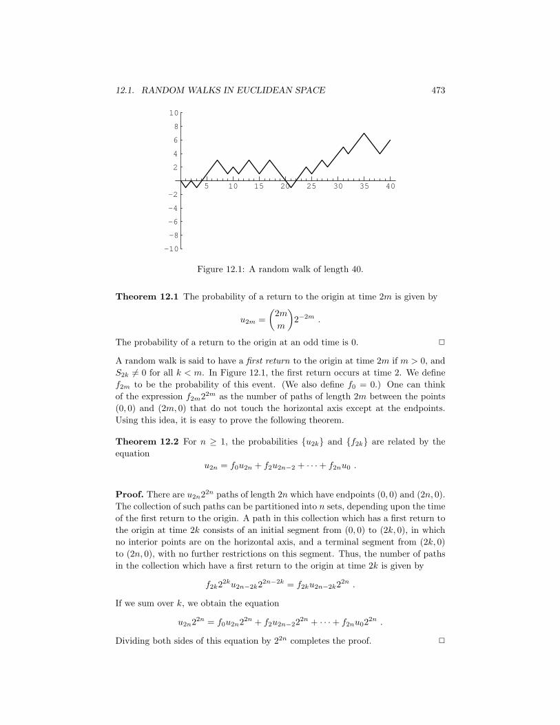
Figure 12.2: Times in the lead.

b2k,2n =12

k∑j=1

f2jα2k−2j,2m−2j +12

m−k∑j=1

f2jα2k,2m−2j

=12

k∑j=1

f2ju2k−2ju2m−2k +12

m−k∑j=1

f2ju2ku2m−2j−2k

=12u2m−2k

k∑j=1

f2ju2k−2j +12u2k

m−k∑j=1

f2ju2m−2j−2k

=12u2m−2ku2k +

12u2ku2m−2k ,

where the last equality follows from Theorem 12.2. Thus, we have

b2k,2n = α2k,2n ,

which completes the proof. 2

We illustrate the above theorem by simulating 10,000 games of Heads or Tails, witheach game consisting of 40 tosses. The distribution of the number of times thatPeter is in the lead is given in Figure 12.2, together with the arc sine density.

We end this section by stating two other results in which the arc sine densityappears. Proofs of these results may be found in Feller.8

Theorem 12.5 Let J be the random variable which, for a given random walk oflength 2m, gives the smallest subscript j such that Sj = S2m. (Such a subscript jmust be even, by parity considerations.) Let γ2k,2m be the probability that J = 2k.Then we have

γ2k,2m = α2k,2m .

2

8W. Feller, op. cit., pp. 93–94.


The next theorem says that the arc sine density is applicable to a wide rangeof situations. A continuous distribution function F (x) is said to be symmetricif F (x) = 1 − F (−x). (If X is a continuous random variable with a symmetricdistribution function, then for any real x, we have P (X ≤ x) = P (X ≥ −x).) Weimagine that we have a random walk of length n in which each summand has thedistribution F (x), where F is continuous and symmetric. The subscript of the firstmaximum of such a walk is the unique subscript k such that

Sk > S0, . . . , Sk > Sk−1, Sk ≥ Sk+1, . . . , Sk ≥ Sn .

We define the random variable Kn to be the subscript of the first maximum. Wecan now state the following theorem concerning the random variable Kn.

Theorem 12.6 Let F be a symmetric continuous distribution function, and let αbe a fixed real number strictly between 0 and 1. Then as n→∞, we have

P (Kn < nα)→ 2π

arcsin√α .

2

A version of this theorem that holds for a symmetric random walk can also befound in Feller.

Exercises

1 For a random walk of length 2m, define εk to equal 1 if Sk > 0, or if Sk−1 = 1and Sk = 0. Define εk to equal -1 in all other cases. Thus, εk gives the sideof the t-axis that the random walk is on during the time interval [k− 1, k]. A“law of large numbers” for the sequence {εk} would say that for any δ > 0,we would have

P

(−δ < ε1 + ε2 + · · ·+ εn

n< δ

)→ 1

as n → ∞. Even though the ε’s are not independent, the above assertioncertainly appears reasonable. Using Theorem 12.4, show that if −1 ≤ x ≤ 1,then

limn→∞

P

(ε1 + ε2 + · · ·+ εn

n< x

)=

2π

arcsin

√1 + x

2.

2 Given a random walk W of length m, with summands

{X1, X2, . . . , Xm} ,

define the reversed random walk to be the walk W ∗ with summands

{Xm, Xm−1, . . . , X1} .

(a) Show that the kth partial sum S∗k satisfies the equation

S∗k = Sm − Sn−k ,

where Sk is the kth partial sum for the random walk W .


(b) Explain the geometric relationship between the graphs of a random walkand its reversal. (It is not in general true that one graph is obtainedfrom the other by reflecting in a vertical line.)

(c) Use parts (a) and (b) to prove Theorem 12.5.

Documents

Random Walks - Dartmouth Collegechance/teaching_aids/books... · Random Walks 12.1 Random Walks in ... The sequence fS ng1n =1 is called a random walk. ... say, after nmoves, with