Embed Size (px)
Citation preview
RAMAN OPTICAL FREQUENCY COMB GENERATION IN HYDROGEN-FILLED
HOLLOW-CORE FIBER
by
CHUNBAI WU
A DISSERTATION
Presented to the Department of Physics and the Graduate School of the University of Oregon
in partial fulfillment of the requirements for the degree of
Doctor of Philosophy
December 2010
ii
“Raman Optical Frequency Comb Generation in Hydrogen-filled Hollow-core Fiber,” a
dissertation prepared by Chunbai Wu in partial fulfillment of the requirements for the
Doctor of Philosophy degree in the Department of Physics. This dissertation has been
approved and accepted by:
____________________________________________________________ Dr. Steven van Enk, Chair of the Examining Committee ________________________________________ Date Committee in Charge: Dr. Steven van Enk, Chair Dr. Michael G. Raymer Dr. Daniel A. Steck Dr. David M. Strom Dr. Andrew H. Marcus Accepted by: ____________________________________________________________ Dean of the Graduate School

iii
© 2010 Chunbai Wu

iv
An Abstract of the Dissertation of Chunbai Wu for the degree of Doctor of Philosophy in the Department of Physics to be taken December 2010 Title: RAMAN OPTICAL FREQUENCY COMB GENERATION IN HYDROGEN-
FILLED HOLLOW-CORE FIBER
Approved: _______________________________________________
Dr. Michael G. Raymer
In this dissertation, we demonstrate the generation of optical Raman frequency
combs by a single laser pump pulse traveling in hydrogen-filled hollow-core optical
fibers. This comb generation process is a cascaded stimulated Raman scattering effect,
where higher-order sidebands are produced by lower orders scattered from hydrogen
molecules. We observe more than 4 vibrational and 20 rotational Raman sidebands in the
comb. They span more than three octaves in optical wavelength, largely thanks to the
broadband transmission property of the fiber.
We found that there are phase correlations between the generated Raman comb
sidebands (spectral lines), although their phases are fluctuating from one pump pulse to

v
another due to the inherit spontaneous initiation of Raman scattering. In the experiment,
we generated two Raman combs independently from two fibers and simultaneously
observed the single-shot interferences between Stokes and anti-Stokes components from
the two fibers. The experimental results clearly showed the strong phase anti-correlation
between first-order side bands. We also developed a quantum theory to describe this
Raman comb generation process, and it predicts and explains the phase correlations we
observe.
The phase correlation that we found in optical Raman combs may allow us to
synthesize single-cycle optical pulse trains, creating attosecond pulses. However, the
vacuum fluctuation in stimulated Raman scattering will result in the fluctuation of carrier
envelope phase of the pulse trains. We propose that we can stabilize the comb by
simultaneously injecting an auxiliary optical beam, mutually coherent with the main
Raman pump laser pulse, which is resonant with the third anti-Stokes field.

vi
CURRICULUM VITAE NAME OF AUTHOR: Chunbai Wu
GRADUATE AND UNDERGRADUATE SCHOOLS ATTENDED: University of Oregon, Eugene, Oregon
Shanghai Jiaotong University, Shanghai, China
DEGREES AWARDED: Doctor of Philosophy in Physics, 2010, University of Oregon
Master of Science in Physics, 2005, University of Oregon
Bachelor of Science in Applied Physics, 2002, Shanghai Jiaotong University
PROFESSIONAL EXPERIENCE: Graduate Research Assistant
University of Oregon 2004 - 2010.
Graduate Teaching Assistant
University of Oregon 2002 - 2003.
AWARDS AND HONORS:
Graduate Research Fellow, University of Oregon, 2004-present
Graduate Teaching Fellow, University of Oregon, 2002-2004
Outstanding Graduate Award, SJTU, 2002
Shih Yu-Lang Memorial Scholarship for Academic Excellence, SJTU, 1999-2001
vii
PUBLICATIONS:
C. Wu, M. G. Raymer, Y.Y. Wang and F. Benabid, “Quantum theory of phase correlations in optical frequency combs generated by stimulated Raman scattering”, accepted by Physical Review A (2010)
Y.Y. Wang, C. Wu, F. Couny, M. G. Raymer and F. Benabid, “Quantum-fluctuation-initiated coherence in multioctave Raman optical frequency combs,” Physical Review Letter 105, 123603 (2010)
C. Wu, E. Mondloch, M. G. Raymer, Y.Y. Wang, F. Couny and F. Benabid, “Spontaneous phase correlations in Raman optical frequency comb generation”, Frontier in Optics/Laser Science Conference 2010
C. Wu, E. Mondloch, M. G. Raymer, Y.Y. Wang, F. Couny and F. Benabid, “Spontaneous phase anti-correlations in Raman optical frequency comb generation”, CLEO/QELS 2010 (QTuA5)
W. Ji, C. Wu and M. G. Raymer, “Slow light propagation in a linear-response three-level atomic vapor”, Journal of Optical Society B 24, 629 (2007)
W. Ji, C. Wu, S. J. van Enk and M. G. Raymer, “Mesoscopic entanglement of atomic ensembles through non-resonant stimulated Raman scattering”, Physical Review A 75, 052305 (2007)
W. Ji, C. Wu and M. G. Raymer, “Quantum statistics of stimulated Raman scattering in optically-pumped Rb vapor", CLEO/QELS 2006 (QMD7)
C. Wu and M. Raymer, “Efficient picosecond pulse shaping by Programmable
Bragg gratings”, IEEE Journal of Quantum Electronics 42, 871 (2006)

viii
ACKNOWLEDGEMENTS
During my many years study in University of Oregon, I owe a lot of sincere
thanks to many people. I would like to first thank my advisor Professor Michael Raymer,
who consistently supported my research and life. He has led me to greatly improve my
skills in writing, presentations and conducting researches. I will always benefit from his
advises and encouragements in my after-graduation life as a scientist and researcher. I
would also like to acknowledge and thank Prof. Steven van Enk for his help and
collaborations in our quantum entanglement project. I thank Prof. Dan Steck for helpful
insights in “everything you want to know” about Rubidium atoms.
I also got numerous help from my labmates and coworkers. Dr. Wenhai Ji taught
me basic optics lab skills. Dr. Andy Funk helped me with regenerative cavity setup
through emails. Erin Mondloch, Cade Gladehill and Kyle Lynch-Klarup assisted me in
setting up HCPCF experiments. Hayden McGuinness was always helpful in discussions
and sharing his inventory of optics. Dr. Brian Smith, Dr. Justin Hannigan, Dr. Guoqiang
Cui, Dr. Cody Leary, Dash Vitullo and Roger Smith always provided me with helpful
insights about physics and research problems. All of them are my good friends and I wish
them well in whatever they are doing or will do.
I would also like to thank Dr. Larry Scatena for his great help in my laser systems.

ix
I have learned a lot of technical skills in lasers while working with him. For other people
who supported me in electronics and machining, I would like to say “thank you”: Cliff
Dax, Kris Johnson, David Senkovich, John Businger and Jeffery Garman.
Living in Eugene for a foreign student would be hard without a great host family.
I am fortune enough to have them supporting me and loving me for years. Mr. James
Jennings and his wife, Ms. Patricia Jennings, have accepted me as part of their family
from the first day I arrived in Eugene. Their daughters’ families, the Thompsons and
Petersons, also give me warm-hearted loves and supports. I remember every thanks-
giving and Christmas dinner that I was invited at their homes. Those were most
treasurable memories in my life.
Finally, I want to thank my wife Jenny. She has been supporting me in everything
she could during this long journey of Ph.d. program. I truly enjoy every moment with her,
and will always love her as I did in the first day we met in middle school.

x
DEDICATION
To my wife Jenny,
My parents,
And Mr. James H. Jennings and his family
– Your love has supported me, truly.
xi
TABLE OF CONTENTS
Chapter Page
I. AN INTRODUCTION TO OPTICAL FREQUENCY COMB ............................... 1
Backgrounds ........................................................................................................... 1 Motivations ............................................................................................................. 5 Overview of Stimulated Raman Scattering ............................................................. 8 Overview of Raman Optical Frequency Comb Generation ................................ 11 Outlines .................................................................................................................. 14
II. THEORY OF RAMAN OPTICAL FREQUENCY COMB GENERATION ...... 17
Spontaneous Raman Scattering Background ....................................................... 17 Stimulated Raman Scattering and Raman Comb Generation ............................. 21 Raman Comb Theory ............................................................................................ 24 An Alternative Approach ...................................................................................... 33 Quantum Entanglement in Stimulated Raman Scattering .................................... 39 Quantum Entanglement between Two Atomic Ensembles .................................. 43
III. SPONTANEOUS PHASE CORRELATIONS IN RAMAN OPTICAL FREQEUNCY COMB GENERATION ........................................................... 48
Phase Correlation between First Order Sidebands .............................................. 48 Mechanism for Phase Locking .............................................................................. 56 Semi-classical Raman Modulator Model .............................................................. 58 Prospects for Ultrashort Pulse Generation ............................................................ 62
IV. OPTICAL RAMAN COMB GENERATION ....................................................... 66
Hollow-core Photonic Crystal Fiber .................................................................... 66 Gas-loading Cell ................................................................................................... 70 Optical Raman Frequency Comb Generation in HCPCF Filled
with Hydrogen Gas .................................................................................. 73
V. EXPERIMENT AND RESULTS OF PHASE CORRELATION MEASUREMENT ............................................................................................. 80
xii
Chapter Page
Energy Statistics of Generated First-order Stokes Field ....................................... 80 Self-coherence of the Comb Lines ........................................................................ 86 Mutual Coherence between First-order Sidebands ............................................... 92 Synchronize Two Cameras .................................................................................... 99 Phase Correlation between First-order Stokes and Second-order
Anti-Stokes Fields ................................................................................... 103 Two-color Experiment ......................................................................................... 105 Phase locking the Raman Comb .......................................................................... 113
VI. CONCLUSIONS ................................................................................................... 118
APPENDICES
A. DETAILED EXPRESSION FOR CALCULATING ANTI-CORRELATION COEFFICIENT ....................................................... 122
B. PULSE MEASURING DEVICE ........................................................................... 124
BIBLIOGRAPHY ............................................................................................................. 133
xiii
LIST OF FIGURES
Figure Page
1.1. Periodic pulse trains produced from mode-lock laser .............................................. 2
1.2. Frequency comb produced by 30 femto-second mode-lock laser with 80 MHz repetition rate ........................................................................................ 3
2.1. Single molecule scattering ....................................................................................... 18
2.2. Energy diagram of Raman scattering ....................................................................... 19
2.3. Energy diagram of inverse Raman scattering ......................................................... 19
2.4. Vibrational and rotational state in bi-atomic hydrogen molecule .......................... 20
2.5. Raman scattering of ensemble of molecules ........................................................... 21
2.6. Stimulated Raman scattering generation ................................................................ 22
2.7. Cascaded Raman scattering process ........................................................................ 23
2.8. Photon occupation number for different output modes under different dispersion conditions. .......................................................................................... 43
2.9. Scheme to generate entanglement between two atomic ensembles ....................... 44
3.1. Pump and first-order Stokes and anti-Stokes mean intensities and their anti-correlation C as functions of local time ..................................................... 53
3.2. First-order Stokes and anti-Stokes mean intensities and their anti-correlation C as functions of phase mismatch ........................................... 54
3.3 Amplitude and phase of quantity ( )( , ) ( , )1Q L E L
............................................... 56
3.4. Synthesized short pulses under different conditions ............................................. 64
4.1. SEM picture of Kagome fiber after it has been cleaved ......................................... 68
4.2. Broad transmission of Kagome fiber ...................................................................... 70
4.3. Detailed drawing of the gas loading cell ................................................................. 72
4.4. Experimental picture of gas loading cell.................................................................. 73
4.5. Experiment setup for observation of Raman optical frequency comb .................... 74
4.6. Temporal shape of ultra-short pulses ....................................................................... 75
xiv
Figure Page
4.7. Hydrogen rotational comb ....................................................................................... 78
4.8. Hydrogen vibrational comb ...................................................................................... 79
5.1. Experiment setup for measuring Stokes pulse energy statistics .............................. 81
5.2. Single-shot first-order Stokes and pump signals ..................................................... 83
5.3. Intensity statistics of first-order vibrational Stokes ................................................. 85
5.4. Intensity statistics of Raman pump. ......................................................................... 86
5.5. Experiment setup for observation of interference fringes from two Raman optical frequency combs .................................................................................... 88
5.6. Two consecutive single-shot interference fringe of first order Stokes recorded on IR line scan camera ........................................................ ................ 89
5.7. Two consecutive Stokes and anti-Stokes interference fringes recorded on IR and visible linescan camera, respectively ........................................................... 94
5.8. Example of extracting phase from Stokes interference fringe by performing sinusoidal fit ........................................................................................................ 95
5.9. Histogram plot showing the probability distribution of the anti-correlation phase ( 1 1 ) .............................................................................................. 97
5.10. Random phases of Stokes and anti-Stokes fields .................................................. 98
5.11. Simultaneous measurement of pump signals on two cameras ............................ 102
5.12. Histogram plot of the phase 1 1 with asynchronous pump .................... 103
5.13. Histogram showing the probability distribution of quantity 1 22 ...... 105
5.14. Energy diagram of two-color experiment ............................................................ 107
5.15. Experiment setup for two-color experiment ........................................................ 109
5.16. Raman spectrum generated in two-color experiment .......................................... 110
5.17. Picture of fiber when two-color experiment is taking place ............................... 111
5.18. Single shot interference fringes of blue pump’s Stokes and red pump’s anti-Stokes ......................................................................................................... 112
5.19. Experiment result of the probability distribution (histogram) of the quantityblue redstokes anti stokes . .......................................................................................... 113
5.20. Phase locking the Raman comb ........................................................................... 115
5.21. Average amplitude of interference fringes as a function of wavelength tuning ................................................................................................................. 117
1
CHAPTER I
AN INTRODUCTION TO OPTICAL FREQUENCY COMB
Backgrounds
Optical frequency comb refers to light whose spectrum, if analyzed in the frequency
domain by spectrometers or other instruments, consists of many discrete, equally spaced,
narrow-width spectral lines [1]. Mathematically, the frequency of the n-th order spectra
line in the comb can be expressed as:
0n repf n f f ,
where repf is the frequency difference between two adjacent comb lines, and 0f is the
offset frequency.
Since time and frequency is one Fourier transform pair, the optical frequency comb is
equivalent to a periodic optical pulse trains in the time domain. For example, ultrafast
(usually shorter than one nano-second) mode-locked lasers that are commonly used in
optical physics laboratory produce such pulse trains, as shown in Figure 1.1 [2].

2
In mode-lock lasers, a gain medium with extremely broad spectral range (typically
larger than 100 nm in wavelength) is placed inside the laser cavity. Once the gain
medium is pumped by a continuous wave (cw) source, there are hundreds of thousands of
longitudinal modes spontaneously and simultaneously excited inside the cavity. The
spectral separation between adjacent longitudinal modes is determined by the round trip
time of the light travelling inside the cavity, and is typically on the order of 100 MHz to 1
GHz. In order to allow all these modes to be built up and eventually lasing in short-pulse
form, a technique called mode-locking is used so that the phases of different longitudinal
modes are coherent and locked [3, 4].
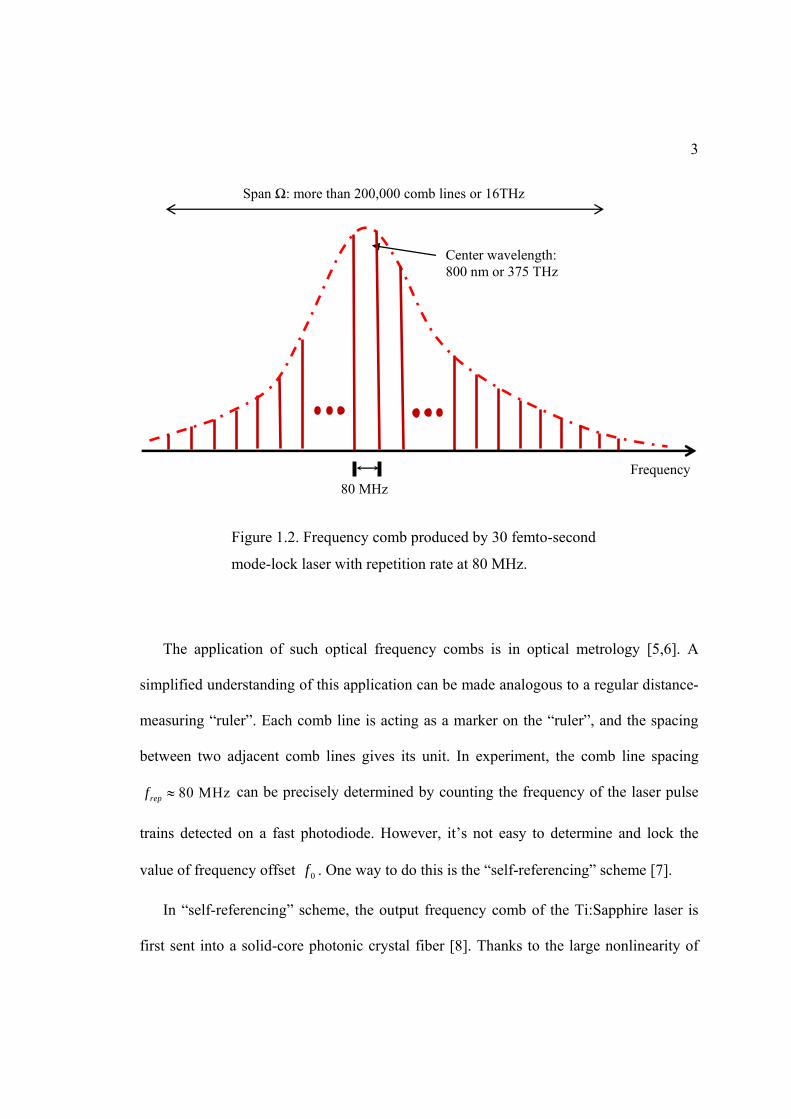
In Figure 1.2, I plot the comb-like spectrum of the output of a 30 femtosecond (10-15 s)
Ti:Sapphire mode-locked laser with repetition rate at 80 MHz. The central wavelength of
the laser output is at 800 nm, and the spectral width is about 16 THz. It therefore contains
more than 200,000 comb lines with spacings equal to 80 MHz.
Figure 1.1. Periodic pulse trains produced from mode-lock laser.
3
The application of such optical frequency combs is in optical metrology [5,6]. A
simplified understanding of this application can be made analogous to a regular distance-
measuring “ruler”. Each comb line is acting as a marker on the “ruler”, and the spacing
between two adjacent comb lines gives its unit. In experiment, the comb line spacing
80 MHzrepf can be precisely determined by counting the frequency of the laser pulse
trains detected on a fast photodiode. However, it’s not easy to determine and lock the
value of frequency offset 0f . One way to do this is the “self-referencing” scheme [7].
In “self-referencing” scheme, the output frequency comb of the Ti:Sapphire laser is
first sent into a solid-core photonic crystal fiber [8]. Thanks to the large nonlinearity of
Figure 1.2. Frequency comb produced by 30 femto-second
mode-lock laser with repetition rate at 80 MHz.
Center wavelength: 800 nm or 375 THz
Frequency 80 MHz
Span Ω: more than 200,000 comb lines or 16THz
4
this kind of fiber, the spectrum of the comb is significantly broadened by the effects such
as “self-modulation” and sum and different frequency generations, so that the comb
spectrum eventually spans more than one octave (factor of two) [9]. In this way the
lower frequency part of the comb can then be frequency doubled in a nonlinear-optical
crystal to spectrally overlap partially with the higher frequency part. The heterodyne
beating frequency detected by a photodiode will then give the value of 0f , and is also
serving as a feedback signal for active locking of the laser cavity. The output of the laser
is then a stabilized frequency comb.
In order to measure an unknown frequency when using the frequency comb, one can
use the comb lines as markers, the same as how we use a ruler to measure distance. The
measurement accuracy, which usually is quantified by the ratio of the measurement
uncertainty f and the absolute frequency f as a unitless number, is extremely small for
the optical frequency comb. For example, a typical Ti:Sapphire femto-second mode-
locked laser will produce a phase-coherent comb whose optical frequency is about 400
THz. The line spacing in the comb equals the repetition rate of the laser, which is
typically set at 80 MHz. After employing sophisticated phase-locking technique, the
measurement uncertainty f can go down to 1 kHz. The ratio between these two numbers
is in the order of 10-13, which is extremely accurate compared with other technologies.
This high accuracy in frequency measurement makes the optical frequency comb
extremely useful in frequency metrology. For example, one can measure the absolute
optical frequency of Cesium D1 line (335 THz or 895 nm) to the resolution of tens of
kHz [10]. In another example, the optical frequency combs directly linked optical

5
frequencies to microwave frequencies beyond five orders of frequency difference, and
thus enables the optical atomic clock at extreme high precision [11]. Physics society has
recognized the importance of research work in optical frequency comb, and awarded the
initial investigators with Nobel Prize [12] in year 2005.
Motivation
We are interested in another application of the optical frequency comb, which is to
synthesize sub femto-second (or atto-second) pulses [13, 14]. Mathematically, the pulse
train given by the optical frequency comb in Figure 1.1 is expressed as:
2 ( )( ) ( ) n ni f tn
n
E t E f e , 0n repf n f f , (1-1)
where n is the phase of individual comb. For simplicity, we assume the phase term is
constant for all comb lines.
It can be shown that the electric field in time domain ( )E t in Equation (1-1) is a
periodic function, and its period is
0 1 / repf ,

6
and, when minimum-duration pulses are created, the width of each pulse (temporal
duration) is directly related to the total frequency span of the comb Ω. A rule of thumb
for the duration is
~ 1/ .
Therefore, a large frequency span of the optical comb could result in extremely short
pulses if all the comb lines are phase coherent. Atto-second pulses are very useful in the
applications of real-time observation and time-domain control of atomic-scale electron
dynamics [15]. One example is by stabilizing the carrier envelope phase of the generated
atto-second pulses, it is possible to create light-induced atomic currents in ionized matter,
and thus control the motion of the electronic wave packets on timescales shorter than 250
atto-seconds [16].
In order to generate atto-second pulses, one needs the spectral span of an optical
frequency comb larger than a few hundred THz. This is out of reach by any active lasing
medium used in mode-lock lasers. In our lab, we generate the optical frequency comb by
using cascaded Raman scattering in hydrogen gas [17]. Many previous works in this
research area employ two independent but phase-stabilized laser pulses to adiabatically
drive the molecular coherence to produce a multiple-octave spanning optical comb [18,
19]. However, we use only a single pump pulse in our experiment. This is an interesting
situation where all the Raman comb lines (except the pump) are spontaneously generated
from the initially zero-photon occupied (vacuum) state. In another words, the generated
Raman comb lines appear to be classical fields, in the sense that they have well defined

7
amplitudes and phases, but they arise from quantum initiation and amplification, which
distinguishes this from the two-pump situation. This argument is also true for the
molecular coherence (vibrational or rotational) created in the hydrogen molecules. From
this point of view, the Raman comb generation process by a single pump is also an
excellent tool to study quantum optics, such as entanglement and quantum fluctuations.
Previous work on Raman scattering theories and experiments has shown that the
generated field from a single Raman pump, which is called the Stokes field, is temporally
and spatially coherent [20, 21], if the scattering takes place in the transient regime and its
Fresnel number is close to unity so the field is diffraction-limited. These two conditions
can be easily satisfied in most Raman scattering experiments. It suggests that the Stokes
field is a transform-limited pulse with a well-defined temporal phase. But in order to
generate atto-second pulses from the optical Raman comb, one must have phase
correlation between those Raman comb components, since in short-pulse synthesis the
frequency components must satisfy certain deterministic phase relationships. Whether or
not such correlation exists is a fundamental question that had not been previously
answered. In this dissertation we will theoretically explore this critical phase correlation
in the transient high-gain regime with no pump depletion. We will show that, for the first
order of Stokes and anti-Stokes, they are very well phase anti-correlated throughout the
duration of these two pulses, even at the situation where large dispersion is induced by a
group velocity difference of Raman sidebands propagating through the media. For higher
order Raman components, we predict their phases are also correlated within one pump
pulse. The result reveals that a short pulse train could be synthesized. However, due to
8
inherent spontaneous initiation of Raman scattering, the generated Raman comb is found
to fluctuate significantly from one pump pulse to another. This fluctuation not only
occurs in the energy of those Stokes or anti-Stokes fields, but also in their temporal
phases. I will show that this fluctuation may change the carrier envelope phase of
synthesize atto-second pulse trains to be random from one shot to another. However,
from our theoretical predictions and experimental evidences, we also find that there is a
new way to lock the random phase to one deterministic value. This will be discussed later.
Overview of stimulated Raman scattering
In order to understand how the optical Raman comb is generated by a single pump
pulse and to see its importance in quantum optics, it is necessary to review the history of
Raman scattering and its applications. The first observations of Raman scattering in
liquids were reported in 1928 [22]. This discovery of “a new radiation” not only
demonstrates the inelastic scattering of light, but opens a new era to explore how light
can interact with matter. This Raman scattering effect was extensively studied by using
natural (sun) light before the invention of laser in 1960, mainly focusing on how it is
different from other optical phenomenon, such as fluorescence and Rayleigh scattering,
and how to determine the scattering cross-section from semi-classical theory [23]. Only
with the strong coherent light that is produced from lasers, the stimulated effect on
Raman scattering was first observed [24]. In this stimulated Raman scattering process,

9
the produced (or frequency-shifted) scattered light, which is usually called Stokes
(frequency down-shifted) or anti-Stokes (frequency up-shifted), reaches a macroscopic
level. Today in industry Raman scattering is well known for its application as “Raman
Spectroscopy” [25], since different materials will scatter light with distinctive frequencies.
This spectroscopic method has been widely used as a basic method for analyzing
chemical compositions of gases, liquids and solids.
The significance of Raman scattering in modern research is its relation to quantum
optics, since by studying the Raman scattering process, it provides answers to some basic
quantum problems, such as how the initial spontaneously scattered photons evolved from
vacuum under the influence of the pump field [26], and what the quantum coherence
property is for the resulting macroscopic field if the stimulated effect is taking place. An
extensive work in this topic was conducted by Dr. Raymer during 1980s [27]. His group
first observed the macroscopic energy fluctuations in the generated Stokes field under
transient high-gain conditions with no depletion of the pump field [21]. He also co-
developed a quantum theory [20] for describing this phenomenon. It was shown that the
energy fluctuation is related to the quantum initiation of the Stokes field, which was also
experimentally shown to be temporally and spatially coherent in later experiments [28].
In recent progress of quantum information experiments, Raman scattering has also
been used as a method to create quantum memory in an ensemble of Raman-active atoms,
such as rubidium or cesium [29, 30]. In those experiments a strong pump laser acted as a
writing tool to interact with the atoms off-resonantly, and the produced Stokes field was
detected to know what “quantum information” has been written into the atomic medium.

10
In the mean-time, the Raman scattering process will also result in the transition of the
atoms between two atomic electronic spin states that are generally not dipole-transition
allowed. In a good approximation, the quantum state of collective electronic spin (CES)
states of all atoms in one medium is entangled with the generated Stokes field, and thus
carries the same “quantum information” as the one that has been written in. This CES
state was demonstrated to be stored up to 1 s in the ensemble and later read-out in a
reverse process, where all the quantum information that was written into the CES state
was transferred into generated anti-Stokes field.
Further application in quantum information is to generate an entangled state between
two distant atomic ensembles [31, 32]. In practice, one atomic ensemble can be treated as
a node in a quantum network. By creating entanglement between them, quantum
information could be relayed through the whole network. Mathematically, the entangled
state of two atomic ensembles means that it cannot be written as the product of CES
states in individual ensembles. To create such entanglement, a writing process using a
Raman scattering scheme is induced in each atomic ensemble. The Stokes fields
generated independently from two atomic ensembles can be entangled by interfering in a
simple optical device, such as a 50:50 beam-splitter. The entangled field states after this
device can be detected, and from quantum theory, after detection the collapsed state of
the two atomic ensembles is then entangled. The generated entanglement then can be
verified by a read-out process. However, until today most such experiments were realized
under the spontaneous regime, which resulted in very few Stokes photons being
generated and detected by single photon detectors, and required an electric-field induced
11
transparency (EIT) scheme [33] to avoid re-absorption of the Stokes photons by the
media. One recent breakthrough [34] has demonstrated quantum memories in Cs
ensemble by using broadband (larger than 1 GHz) optical pulses, instead of megahertz
modulated cw lasers.
Overview of Raman optical frequency comb generation
As shown in Figure 1.1, the mode-locked lasers generate ultrashort optical pulses by
establishing a fixed phase relationship across their spectrum of frequency. However, the
frequency span of the comb generated by these lasers is typically no larger than 20 THz.
Most experiments using optical combs to do absolute frequency measurements, such as
atomic clocks and attosecond control of electronic processes, require the comb spectra to
a have multiple-octave span. As described in the previous section, one way to generate
such a broad spectrum is using photonic crystal fiber that has large nonlinear effects like
four-wave mixing or self-phase modulation.
Alternatively, discrete Raman combs from molecules are studied in many recent
research efforts that aim to synthesize sub-femto or atto-second optical pulses. In this
scheme, a cascaded Raman scattering process is induced under certain conditions. The
generated first-order Stokes and anti-Stokes fields, which are co-propagating with the
intense pump light, will be scattered by the molecules again to produce higher order
sidebands. Therefore, the frequency comb generated will have a similar spectrum as
12
shown in Figure 1.2. The Raman shift in the medium determines the frequency difference
between two adjacent comb lines, which, in a mode-locked cw laser, is controlled by its
resonator length. This Raman shift is quite large, for example, in hydrogen molecules, the
rotational Raman shift is 18 THz, and the vibrational Raman shift is about 125 THz.
The first experiment to explore the Raman comb generation is done in hydrogen gas
when multiple rotational lines are observed and analyzed under high-power femto-second
pulses [17]. Shortly after that experiment a two-pump scheme is proposed [35] where the
Raman coherence is driven slightly off resonance and results in the Raman spectrum with
Bessel-function amplitudes and phases. Experiments following this scheme successfully
produced single-cycle optical pulses by adjusting the relative phase between each comb
component [18]. Further efforts in controlling the carrier envelope phase of the generated
single cycle pulse [19, 36], as well as to generate constant shape pulse trains [37], have
been realized. Other experimental schemes, such as using ultra-short pulses to generate
impulsive Raman coherence, also show promising phase locking effect between Stokes
and anti-Stokes components.
In another hand, micro-structured hollow-core fiber (HCF) has been developed [38],
and it shows broad transmitting optical band which is even larger than one octave. For a
typical step-index fiber, the optical modes are confined inside the core area with higher
refractive index than that of the cladding materials. No optical modes can be guided when
the core is hollow for this kind of fiber. However, in micro-structured HCF, its cladding
is constructed in a way that resembles the periodic structure of a two-dimensional crystal
lattice. Indeed, an easy picture to see how the light is confined inside the fiber where a

13
large air hole is surrounded by such cladding structure is by the Bragg reflections off the
periodic crystal lattice. Using the similar theory that is used in solid-state physics to
describe the crystal structure, one can calculate the photonic band-gap which determines
the guided wavelength of such fiber.
Since the core area of the HCF fiber is hollow, one can fill it with different gases
under various pressures. If strong laser light is coupled into such fiber, cascaded Raman
scattering may take place, creating a Raman optical frequency comb [39]. Using fiber in
generating Raman combs has two major advantages compared with the conventional
free-space Raman experiments: first, a Raman active medium like hydrogen gas can be
pressure sealed inside the core area of the fiber and thus strongly interact with coupled
pump light. Second, since the core diameter of most HCF fiber is about 10 microns, the
pump light is tightly focused when transmitting inside the fiber. This ensures the pump
intensity as well as the Raman interaction region are extremely larger compared with the
conventional free-space Raman experiments using a long-focal-length lens to focus the
pump.
For an example, in our lab, we generate more than 20 Raman rotational lines in
hydrogen gas when coupling a Raman pump into the gas-filled HCF fiber. The power of
the Raman pump is about 10 micro-joules per pulse, which is very low compared to the
power required in a free-space setup, usually at 10 millijoules.
14
Outlines
In this dissertation, I will focus on the discussion of the phase relationship between
comb lines in Raman optical frequency comb generation. I will first show how we predict
this phase relationship by using both classical and quantum models. Then the
experimental setup that allows us to generate Raman combs and verify this phase
relationship will be covered. In the last part, I will discuss a proposal for how to lock
more strongly the phases of comb lines based on our theory and observations.
In Chapter II, I start with the description of how a single molecule or atom interacts
off-resonantly with light to produce frequency-shifted Stokes and anti-Stokes photons. I
then discuss the stimulated Raman scattering process in a molecular ensemble, and a
possible cascade process that produces many orders of Stokes and anti-Stokes lines. In
order to connect established Raman scattering theory with cascaded Raman scattering
effect which produces optical Raman frequency comb, we take all orders of Stokes and
anti-Stokes fields into consideration. By following the method adopted in [40], we first
adiabatically eliminate the molecular intermediate states from the interaction Hamiltonian,
and then use optical Maxwell-Bloch theory to derive the equations of motion for all
Stokes and anti-Stokes fields, as well as the buildup of the molecular coherence. We also
develop an alternative approach where the propagations of Stokes and anti-Stokes fields
are derived directly in the quantum Heisenberg picture, and find the same equations of
motion. In the last part of this Chapter, I will discuss that in stimulated Raman scattering
process where only first order Stokes is present, the Stokes field and molecular coherence
15
are created in an entangled state. This special property of Raman scattering has been used
to generate entanglement between two distant atomic ensembles.
In Chapter III, the analytical solution of the equations of motion involving only first-
order Stokes and anti-Stokes in a quantum model is shown. The numerical evaluations of
these solutions based on quantum initiation conditions are then used to calculate the
newly defined phase anti-correlation coefficient. We show that this coefficient is directly
related to the intensity and phase fluctuations of first-order Stokes and anti-Stokes fields.
Our calculation result then predicts that the phases of first-order Stokes and anti-Stokes
are nearly perfect anti-correlated, which means the sum of their phases remains constant
from shot to shot. Following this prediction, a semi-classical non-perturbative theory
assuming that excited molecules act as a phase modulator is used to show that there exists
a deterministic relation between phases of all comb lines in a single shot.
In Chapter IV, the experiments to generate a Raman optical frequency comb in
hydrogen-filled hollow-core photonic crystal fiber (HCPCF) are presented. First, I briefly
describe the manufacturing procedures and guiding mechanisms of HCPCFs that are
made in University of Bath, UK. Then I show our own design of gas loading cell that is
capable to fill the hollow-core fiber with controllable pressure gases. Most parts of this
gas loading cell use commercially available parts, and require very little machining. It
also shows the advantages of easy assembly and high pressure sealing. Next, I will
describe our laser system, which consists of a mode-locked Ti:Sapphire laser producing
nearly Fourier-transform-limited pulses with 200 pico-seconds temporal duration and a
one-stage amplification system (regenerative amplifier). The amplified pulse is then used
16
as a Raman pump to couple into HCPCF filled with hydrogen gas. Depending on the
polarization state of the Raman pump, I show the observed hydrogen rotational or
vibrational optical combs.
In Chapter V, I will show the setup of a two-fiber experiment that will directly
measure the phase correlation between comb lines. The experimental results and the data
analysis will be covered as well. We emphasize the observed strong spontaneous phase
anti-correlations between first-order sidebands, which are consistent with our theoretical
predictions. A weaker phase correlation between first-order Stokes and 2nd order anti-
Stokes is also shown. I will then describe a two-color experiment that verifies the phase
correlations predicted by our semi-classical model. In this experiment the second
harmonic (in blue color) of amplified pulse (in red color) generated in a BBO crystal and
the amplified pulse itself are simultaneously coupled into HCPCF. This blue light is kept
in low intensity so that it is only scattered off the molecular coherence created by the red
light. The experimental results reveal that the molecular coherence is indeed acting as a
phase modulator for light scattering from it. At the end of this chapter, I will discuss the
possibility to extend the two-color experiment to lock the phase of Raman comb, which
will be crucial to generate atto-second pulse trains with constant carrier envelope phases.
I will summarize my research work in the last chapter of this dissertation.

17
CHAPTER II
THEORY OF RAMAN OPTICAL FREUQUENCY
COMB GENERATION
Spontaneous Raman scattering background
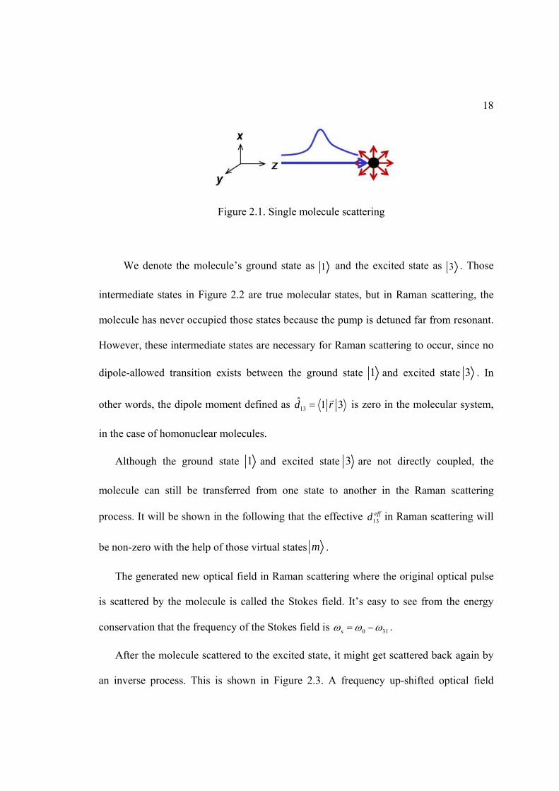
As shown in Figure 2.1, an optical pulse propagating at z direction encounters a single
molecule in its ground state. If the frequency of the optical pulse is far detuned from any
transition line of the molecule, an inelastic scattering may occur where the frequency of
the optical pulse is shifted and the molecule is transferred to its excited state. This is the
well-known spontaneous Raman scattering process. The energy diagram of the described
Raman transition is shown in Figure 2.2. In our theoretical model, we assume the optical
pulse to be quasi-monochromatic, and its temporal duration is shorter than the Raman de-
phasing time, but its spectral linewidth is much narrower than the Raman frequency shift.
Under these conditions, the Raman scattering process is in transient regime.
18
We denote the molecule’s ground state as 1 and the excited state as 3 . Those
intermediate states in Figure 2.2 are true molecular states, but in Raman scattering, the
molecule has never occupied those states because the pump is detuned far from resonant.
However, these intermediate states are necessary for Raman scattering to occur, since no
dipole-allowed transition exists between the ground state 1 and excited state 3 . In
other words, the dipole moment defined as 13ˆ 1 3d r
is zero in the molecular system,
in the case of homonuclear molecules.
Although the ground state 1 and excited state 3 are not directly coupled, the
molecule can still be transferred from one state to another in the Raman scattering
process. It will be shown in the following that the effective 13effd in Raman scattering will
be non-zero with the help of those virtual states m .
The generated new optical field in Raman scattering where the original optical pulse
is scattered by the molecule is called the Stokes field. It’s easy to see from the energy
conservation that the frequency of the Stokes field is 0 31s .
After the molecule scattered to the excited state, it might get scattered back again by
an inverse process. This is shown in Figure 2.3. A frequency up-shifted optical field
Figure 2.1. Single molecule scattering

19
called the anti-Stokes field is produced during this process. The anti-Stokes field will
have frequency 0 31as .
The energy structures of real molecules are very complicated, since there are many
possible degrees of freedoms in its Hamiltonian, such as electronic, nuclear vibration and
rotation, inter-molecular and so on. However, in order to discuss Raman scattering, we
could simplify the energy structure to a few levels whose transition will have the largest
Raman scattering cross sections. For example, in hydrogen molecules, the most
significant Raman scattering takes place involving the vibrational and rotational states
between two hydrogen atoms (shown in Figure 2.4). All other states, such as electronic,
will be treated as intermediate states. In this simplified model, the energy structure of
Figure 2.3. Energy diagram of
inverse Raman scattering
Figure 2.2. Energy diagram of
Raman scattering

20
molecules is essentially a system. Both the ground state 1 and excited state 3 are
assumed to be degenerate, which means a single wave-function is sufficient to describe
each state.
The energy separation between ground state 1 and excited state 3 is 13E .
At room temperature, for BE k T where Bk is the Boltzmann constant, the molecule
will naturally be in its ground state. However, if that condition is not met, the molecule
will have near-equal probability in its ground or excited state. In this situation, the optical
Raman gain will be diminished. An optical pump scheme is required so that the molecule
is prepared in its ground state.
Figure 2.4. Vibrational and rotational state in bi-atomic hydrogen molecule

21
Stimulated Raman scattering and Raman comb generation
Now we consider an ensemble of molecules that is confined within a pencil-shaped
container. As shown in Figure 2.5, an optical pulse propagating along the length of the
container interacts off-resonantly with these molecules. Each molecule can experience
the spontaneous Raman scattering process to produce the Stokes field, as described in the
previous section. In certain conditions, especially when the optical pulse, which is called
the Raman pump, is intense enough, the spontaneous scattering can build up to generate a
strong Stokes field that is co-propagating with the original optical pulse. This
phenomenon is called stimulated Raman scattering.
One simple way to understand the stimulated process is as follows: the Stokes fields
spontaneously generated from the first few molecules in the ensemble interacting with a
strong Raman pump are distributed uniformly for each propagation direction. However,
the Stokes field that happened to be propagating co-linearly with the pump laser may
stimulate the scattering process occurring in the next available molecules. Here,
“stimulate” means the first Stokes field, as shown in the leftmost event in Figure 2.6,
Figure 2.5. Raman scattering of an ensemble of molecules (Blue curve indicates
Raman pump, and red curve indicates generated Stokes field)

22
forces the next Raman scattering effect to produce a Stokes field with an identical
property, i.e., the propagation direction, the wavelength and temporal phase. In other
words, the Raman pump laser set a preferable direction where the Stokes fields from
sequential spontaneous Raman scattering will be produced coherently. This is very
similar to how lasers work. This stimulated Raman scattering process will continue until
the Raman pump is depleted and the Stokes field could build up to a macroscopic level
(larger than one million photons).
Molecules that are scattered to an excited state in the stimulated Raman scattering
process can be scattered back by the same pump pulse to produce anti-Stokes photons
(see Figure 2.3). Similar to the Stokes field buildup, the anti-Stokes field can also reach
macroscopic level. The generation of both Stokes and anti-Stokes photons can be made
analogous to a four-wave mixing process, where two pump photons are annihilated, and
Stokes and anti-Stokes photons are generated. In this process, there exists a phase
mismatch, i.e., 02s as , where s , as , 0 are the wave-vectors of Stokes,
anti-Stokes and Raman pump fields, respectively. It has been shown that in a perfect
phase-matching condition, the Stokes and anti-Stokes processes will be suppressed, while
Figure 2.6. Stimulated Raman scattering generation

23
for small but nonzero phase mismatch it will be enhanced. We will point this out in a
later chapter.
After this Stokes field gets stronger, it might be scattered by the molecules again to
produce higher-order sidebands. The same will happen to the anti-Stokes fields. This
cascaded process is what we call “Raman comb generation.” In Figure 2.7 we show this
process. Because in our experiment we use very short (200 ps), high-intensity laser pulses
to excite the Raman scattering, we will focus our theoretical discussion in a high-gain
transient regime. In the following section, I will show how we obtain the equations of
motion of the slowly varying parts of the radiation fields (including all Raman comb lines)
and the collective molecular coherence.
Figure 2.7. Cascaded Raman scattering process
24
Raman comb theory
We start our mathematical derivation with the quantum theory of Raman scattering,
which will generalize to include any number of Raman lines in comb generation process
[40]. Consider a single molecule located at position z and its interaction with all electric
fields containing the pump and generated Raman sidebands. We write the electric fields
as:
( )( ) ( , ) . .n ni z tn
n
E E z t e h c (2-1)
where we label integer number n as the order of sidebands, n<0 for Stokes fields, n>0 for
anti-Stokes fields, and n=0 for the pump. We will keep this convention of naming the
order of Stokes and anti-Stokes fields throughout the rest of this dissertation. ( ) ( , )nE z t is
the positive frequency part of the slowly varying envelope function. This envelope
function is directly related to the photon creation and annihilation operators in quantum
optics, and we will show its real form in the next section. The carrier frequency n in the
expression for the different order of the Stokes (anti-Stokes) line obeys the energy
conservation, and it is related to the pump’s frequency by:
0 31n n , (2-2)
In other words, the generated spectrum of cascaded Raman scattering process would be
an equally spaced optical frequency comb. The parameter n is the wave-vector of the n-
25
th order sideband, and its value is mainly determined by the dispersion property of the
medium.
The total Hamiltonian that will determine the molecule’s equation of motion can be
written as (neglecting free radiation fields):
0mol
IH H H , (2-3)
In the above equation, 0mol
mm
H m m is the molecule’s static Hamiltonian,
and
1 1 3 3 ( ) ( , ) ( ) ( , ) . .I m m m m
m
H d t E z t d t E z t h c (2-4)
is the dipole interaction Hamiltonian between the molecule and the electric fields of light.
The operator ,m n m n is the molecular transition operator between state n and
m . If the zero of energy is taken at the level of the ground state, the static Hamiltonian
can be re-written as 0 1 1 1( ) ( )mol
m m mm
H t t , where 1 1m m .
We then obtain the equations of motion for molecular operators that involve states
1 , 3 and m in the Heisenberg picture (neglect any transition between intermediate
states):
31 31 31 1 3 3 1m m m m
m m
i i d E i d Et
, (2-5-1)

26
1 1 1 1 11 3 31( )m m m m mm mi id E id E
t
, (2-5-2)
3 3 3 3 33 1 31( )m m m m mm mi id E id E
t
. (2-5-3)
In our transient Raman scattering theory, we assume the laser is detuned far away
from the intermediate states, that is, 0m
Ed
. In this situation, the molecule is
assumed to never truly occupy those intermediate states m during the interaction.
Therefore, we would like to eliminate these intermediate states from our equation of
motion. In order to do so, we need to apply some essential approximations, and next, I am
going to show this derivation in some detail. The first term of Equation 2-5-1 reads:
31 31 31( ) ~t i
t
. (2-6)
This shows the operator 31( )t is oscillating at its natural frequency 31 . Any temporal
oscillating term appearing in its equation of motion that has a frequency other than 13
may be neglected (or have negligible contribution).
We can formally integrate Equation 2-5-2 and 2-5-3 and get:
1 1 31( ) ( )1 1 1 11 3 310( ) (0) ( )[ ( ) ( )] ( ) ( ) m m
ti t i t t i t tm m m mm mt e i dt e d E t t t d E t t e ,
(2-7-1)
3 3 31( ) ( )3 3 3 33 1 310
( ) (0) ( )[ ( ) ( )] ( ) ( ) m mti t i t t i t t
m m m mm mt e i dt e d E t t t d E t t e ,
(2-7-2)

27
These expressions for 1( )m t and 3 ( )m t can then be put into Equation 2-5-1 and only
the terms that have 31i te need to be retained. For example, the third term in Equation 2-7-
1 can be written as:
1
1
1 31
3 1 3 1
( )3 1 110
2 ( ) ( )3 310
( ) (0)
( ) ( )[ ( ) ( )]
( ) ( ) ( )
m
m
m
i tm m m m
m m
t i t tm m mm
m
t i t t i t tm
m
i d E i d E t e
d d E t dt e E t t t
d E t dt e E t t e
In the above equation, the first term proportional to 1(0)m is oscillating at 1m , and
can be neglected. The third term, which is proportional to 31( )t itself, is a term directly
resulting in AC Stark shift. It only slightly shifts the frequency 31 and is also negligible.
The only term that might have oscillation at 31 is the second term, and by using Equation
2-1, we can get:
1
1 0 1 2 0 2
1 2
1 2
( )3 1 1 3 0
( ) ( )( ) ( )11 ( , ) . ( , ) . [ ( ) ( )]
m
n R n R
t i t tm m m m
m m
i z i n t i z i n tn n mm
n n
i d E d d dt e
E z t e h c E z t e h c t t
(2-8)
Here we use the Rotating-wave approximation (RWA) to neglect terms involving
t t . This will allow us to simplify the double summation in (2-8) as:
28
1 0 1 31 2 0 2 31
1 2
1 2
0 1 2 31 2 1
1 2
1 2
( ) ( )( ) ( )11
( ) ( ) ( )( ) ( )11
( )1
( , ) . ( , ) . [ ( ) ( )]
( , ) ( , ) . [ ( ) ( )]
( , )
n n
n n
i z i n t i z i n tn n mm
n n
i t t i n t n t i zn n mm
n n
n n
E z t e h c E z t e h c t t
E z t E z t e e e h c t t
E z t E
0 31 0 31 31( ( 1) )( ) ( )( )( ) ( ) ( )
1
11
( , ) ( , ) ( , )
[ ( ) ( )]
ni n t t i n t t i z i tn n
n
mm
z t e E z t E z t e e e
t t
.
(2-9)
where 1n n n .
Again, since operator 31( )t is oscillating at frequency 31 , in the second step of the
above derivation we eliminate one summation to only retain the term 31i te . By putting
this result back into Equation 2-8, and making the adiabatic following approximation
since the slowly varying envelopes ( , )nE z t , operators 33( )t and ( )mm t are all slowly
changing compared with the frequency 1m , we have:
1
0 31 0 31 31
31
( )3 1 1 3 0
( ( 1) )( ) ( )( )( ) ( ) ( ) ( )1 1
11
( ) ( )1
( , ) ( , ) ( , ) ( , )
[ ( ) ( )]
( , ) ( , )
m
n
n
t i t tm m m m
m m
i n t t i n t t i z i tn n n n
n
mm
i z im n n
i d E d d dt e
E z t E z t e E z t E z t e e e
t t
i E z t E z t e e
11[ ( ) ( )]tmm
n m
t t
(2-10)
where we define 3 11 0 31 1 0 31
1 1
( 1)m m mm m
d dn n
.
In a similar way, we can get the second term in equation 2-5-1 as:
31( ) ( )1 3 1 33( , ) ( , ) [ ( ) ( )]ni z i t
m m m n n mmm n m
i d E i E z t E z t e e t t . (2-11)

29
Finally, by using equations 2-10 and 2-11, we simplify equation 2-5-1 as:
31( ) ( )31 31 31 1 11 33( ) ( ) ( , ) ( , ) [ ( ) ( )]ni z i t
m n nn m
t i t i E z t E z t e e t tt
(2-12)
Since we assume the molecule initially in its ground state, and the probability of the
molecule staying in state 3 is very small, that means 11 33 1 remains valid
throughout the interaction. Therefore, Equation (2-12) is further simplified as:
31* ( ) ( )31 31 31 1, 1( ) ( ) ( , ) ( , ) ni z i t
n n nn
t i t i E z t E z t e et
(2-13)
where the Raman transition coefficient is given by:
1, 3 11 0 31 1 0 31
1 1
( 1)n m mm m m
d dn n
. (2-14)
We define the slowly varying part of operator 31( )t as another variable QK:
31
31( ) ( ) i tQ t t e . (2-15)
Here we use symbol to denote the different molecule located at position z. The
physical meaning of QK(t) is the slowly varying molecular-raising operator, which
eliminates one molecule initially in ground state 1 and at the same time, creates one
30
molecule in excited state 3 . Its equation of motion can easily be derived from Equation
2-13:
* ( ) ( )1, 1( ) ( , ) ( , ) ni z
n n nn
Q t i E z t E z t et
(2-16)
The above equation describes the response of a single molecule at location z to the
electric fields. Next, we consider an ensemble of molecules that are assumed to be evenly
distributed in a pencil-like region, as shown in Figure 2.5, with the length L in z direction,
area A in the cross-section and the molecule’s number density N. In our theory, we
assume the Fresnel number of the interaction, defined as A
L, is smaller than unity for all
optical fields. For this reason, a one-dimensional model is sufficient for modeling the
cascaded Raman process.
In order to treat the propagation of the radiation field, it is convenient to define the
collective molecular raising operator at position z by:
1( , ) ( )
z
Q z t Q tN
, (2-17)
where the summation runs for all molecules that are occupied at position z. People often
refer to Q as the molecular collective coherence.
The commutation relation for ( , )Q z t and † ( , )Q z t can be found as:

31
† 1( , ), ( , ) ( )Q z t Q z t z z
NA (2-18)
We can rewrite Equation 2-16 as:
* ( ) ( )1, 1( , ) ( , ) ( , ) ni z
n n nn
Q z t i E z t E z t et
. (2-19)
Next, we will calculate the macroscopic polarization operator, which is defined as:
( , ) ( ) ( )P z t P t z z
, (2-20)
where ( )mP t is the polarization arising from single molecule located at position mz :
1 1 3 3( ) . .m m m m
m
P t d d h c . (2-21)
We can evaluate the above polarization by using Equation 2-5, which also uses
similar adiabatic approximations:
1 ( ) * ( )1, 1 1
( )( ) ( )1, 1
†( ) ( , ) ( )
( , ) ( ) . .
n n n
n n n
i z i z tn n
n
i z i z tn n
n
P t E z t Q t e e
E z t Q t e e h c
( )
, (2-22)
Using equation 2-22, the macroscopic polarization ( , )P z t can be written as:

32
1 ( )* ( )1, 1 1
( )( )1, 1
†( , ) ( , ) ( , )
( , ) ( , ) . .
n n n
n n n
i z i z tn n
n
i z i z tn n
n
P z t N E z t Q z t e e
N E z t Q z t e e h c
. (2-23)
This macroscopic polarization can be used to calculate the equation of motion that
accounts for the spatial propagation of the electric fields in the Raman comb generation
process. The well-known one-dimensional Maxwell-Bloch equation is:
2( , )E P z t
z c t c t
, (2-24)
Then using equation 2-23 for ( , )P z t and equation 2-1 for E , and sorting out the term
with fast optical oscillation n , the equation of motion for the n-th order comb line can
be found from equation 2-24 as:
1( ) ( ) ( )2, 1 1 2, 1
†1( , ) ( , ) ( , ) ( , ) ( , )n ni z i z
n n n n nE z t i E z t Q z t e i E z t Q z t ez c t
(2-25)
where the coefficient 2, 1,2 /n n nN c .
Equations 2-19 and 2-25 will be the coupled equations describing the Raman comb
generation.
33
An alternative approach
In the previous section, we started with the single molecule’s interaction with light
and then derived the equation of motion for the slowly varying collective molecular-
raising operators and the electric fields. Although we write the electric fields in standard
quantum optics operators, we derive their equations from the Maxwell-Bloch theorem, a
corollary from quantum mechanics and Maxwell equations. In this section, we use a
different approach where the basic quantum theory – the dynamics of a quantum operator
in the Heisenberg picture – is used. This approach will be useful in the future
development of the Raman theory because of its simplicity and clearness.
We first quantize the radiation field in free space, which can be found in a standard
textbook. It starts with the transverse part of the potential vector in Coulomb gauge in
terms of normal modes. In our situation where only one propagation dimension (along the
z axis) is considered, then the normal modes will have wave vectors being quantized as
2, 0, 1, 2,...n n
L
. The quantized electric field can be written as:
2( , ) .m mi z i tm
x mm
E z t i a e h cAL
(2-26)
where x labels the polarization of the electric field, A and L are the area (assume
uniformity along z) and length of the molecular medium. The operator ma is the photon
34
annihilation operator that is similar to the one used in the quantum-mechanic harmonic
oscillator and the commutation of ma and na obeys:
,†,m n m na a . (2-27)
If L , the discrete summation of all normal modes may be re-written in
continuous integration, by changing
2
( ) ; 2m
m
La a dm d
L
. (2-28)
In this way, the commutation for ( )a and † ( )a is:
†( ), ( ) ( )a a (2-29)
Then using 2-28, the quantized electric field is:
( )( )( , ) ( ) .i z i t
xE z t i d a e c cA
. (2-30)
We are more interested in the slowly varying envelope of a n-th order Raman
sideband that has center frequency n and wave-vector n . Therefore, we re-write the
quantized electric field in following form:
( )( )( , ) ( , ) .n ni t zx n
n
E z t E z t e c c (2-31)

35
and the slowly-varying envelope for n-th order sideband is given as:
( ) †( , ) (1 ) ( )2
gn
gi z iv tn n
n nn
vE z t i d a e
A
, (2-32)
where gnv is the group velocity of the n-th order sideband. In deriving equation 2-32, we
have used the dispersion relation as ( ) gn n nv , and have changed the
integration variable in equation 2-31 to small wave-vector spreading around n .
The total Hamiltonian of the radiation field in free space is given by:
22
0 ( ( , ) ( , ) )8
radx y
AH dz E z t B z t
(2-33)
By putting into the full expression for the electric (equation 2-31) and magnetic fields,
it can be shown that the above Hamiltonian can be simplified as:
0
† † ( ) ( ) ( ) ( )2
rad gn n n n
nnH d v a a a a
. (2-34)
From equation 2-32, the slowly varying envelope can be written approximately as:
( ) 0 †( , ) ( , )n nE z t i a z tA
, (2-35)
if we define the new photon creation and annihilation operator as:
36
† †( , ) ( )
gni k z ivv k t
n na z t d k a k e (2-36)
The Fourier inverse transform of above equation would give:
† †1( ) ( , )
2
gni kz iv k t
n na k dzdt a z t e
(2-37)
Then, the free-space Hamiltonian in Equation 2-34 can be expressed in a different
way:
1 2
1 2
1 2
2
0 1 1 2 2
1 1 2 22
11 2 22
1
†
†
†
1( , ) ( , )
2 2
( , ) ( , )8
( , )( , )
8
n ng gi z iv t i z iv trad n
g n nn
i z i zng n n
n
i z i zn ng n
n
H d v dz a z t e dz a z t e
d v dz a z t e dz a z t e
a z td v dz e dz a z t e
z
†( , )( , )
4n ng n
n
a z tdzv a z t
z
(2-38)
We can further write this Hamiltonian in terms of the slowly varying operator
( , )nE z t , by using the inverse of equation 2-35:
( )( )
0
( , )( , ) . .
4rad n
nn n
ic E z tH Adz E z t h c
z
(2-39)
if we assume the group velocities of all the electric fields in free space are at the speed of
light in a vacuum, c. This form is consistent with, but generalizes, that in Haus [41].
37
The commutation between the positive and negative frequency part of the slowly
varying envelope can be easily found from equation 2-45, and take the form as:
( ) ( ) 02( , ), ( , ) ( ( ))n m nmE z t E z t z z c t t
A
(2-40)
The interaction Hamiltonian between the radiation field and the single molecule at
position z is given by equation 2-4, and if we include all molecules, then the interaction
Hamiltonian can be formally written as:
1 1 3 3
( ) ( , ) ( ) ( , ) . .I m m m mm
H A dz d t E z t d t E z t h c
(2-41)
Again, we use the adiabatic-following approximation to eliminate those intermediate
states m from the above interaction Hamiltonian. To do so, the expressions for 1( )m t
and 3 ( )m t that are shown in Equation 2-5 are put into the Hamiltonian, and a similar
approach to that in the previous section is applied to only retain those slowly varying
terms, then the interaction Hamiltonian can be shown as:
1
1, 1
*1, 1 1
†
( ) ( , ) ( , ) ( , )
( , ) ( , ) ( , )
n
n
i zI n n n
n
i zn n n
H NA dz Q z t E z t E z t e
Q z t E z t E z t e
(2-42)
Combining Equation 2-39 and 2-42, the total Hamiltonian of our system is
0rad
IH H H . The molecular static Hamiltonian molH is not included in H because it is
eliminated when we do the slowly varying transformation from 13( )t to ( , )Q z t

38
(Equation 2-15). Indeed, the Hamiltonian H is in the interaction picture. The equation of
motion for slowly-varying electric field operator of n-th order comb component can be
easily obtained from standard quantum theory:
( ) ( )
0( , ) , ( , )radt n I nE z t i H H E z t (2-43)
Using the commutation relations that are shown in Equation 2-25 and 2-50, the above
equation can be simplified as:
( ) ( ) ( )2, 1 1 1 2, 1
†1( ) ( , ) exp( ) exp( )z t n n n n n n nE z t i E i z Q i E i z Q
c
(2-44)
The new coefficient 2 ,n is given by: 2, 1,2 /n n nN c .
The equation of motion for the collective molecular raising operator can be obtained
in a similar way:
1
†0
( ) ( )1, 1
* ( ) ( )1, 1 1
( ) ( )1, 1
†
† †
( , ) , ( , )
( ) ( , ) ( , ) ( , )
( , ) ( , ) ( , ) , ( , )
exp( )
n
n
radt I
i zn n n
n
i zn n n
n n n nn
Q z t i H H Q z t
i NA dz Q z t E z t E z t e
Q z t E z t E z t e Q z t
i E E i z
(2-45)
It is easy to see that the equations of motion that we derive in this section are the
same as those we get in the previous section (Equation 2-19 and 2-25). By changing the
variable from ( , )z t to ( , )z , where /t z c , the equations of motion become:

39
( ) ( ) ( )
2, 1 1 1 2, 1†( , ) exp( ) exp( )z n n n n n n nE z i E i z Q i E i z Q
, (2-46)
( ) ( )1, 1
† ( , ) exp( )n n n nn
Q z i E E i z . (2-47)
These two equations will be our starting point to make the theoretical predictions on
interesting features in the Raman optical frequency comb generation process, which will
be discussed in the next chapter.
Quantum entanglement in stimulated Raman scattering
During the optical Raman frequency comb generation, the collective molecular
coherence ( , )Q z t and optical comb components nE are initiated from a vacuum state,
and then amplified to a macroscopic level. Equations 2-46 and 2-47 describe this process.
However, an interesting question is whether the collective molecular coherence has
special correlations with those electric fields. In this section, I will review this special
correlation, which in a later context will be shown as quantum entanglement, under the
condition that only first-order Stokes is generated.
The interaction Hamiltonian that involves only first-order Stokes and Raman pump
can be written directly following Equation 2-42:
01,0 0 1( ) ( , ) ( , ) ( , ) . i z
IH NA dz Q z t E z t E z t e h c
40
Since the Raman pump is assumed to be a strong laser field, we write its form 0E
classically instead of in a quantum operator. Using the above Hamiltonian or Equation
(2-46) and (2-47), the equations of motion for first-order Stokes and molecular collective
coherence are:
0( )
1 2,0 0†( , ) ( ) ( , ) i zE z i E Q z e
z
,
0( )
1,0 0 1† ( , ) ( ) ( , ) i zQ z i E E z e
. (2-48)
After doing a complex conjugation of the first equation above, absorbing dispersion
factor 0 z into 0( )E , and defining parameters: ( )1 1
1
ˆ ( , ) ( , )2
Aca z t E z t
as a Stokes
photon annihilation operator, 10
2 Ng
c
as a normalized gain coefficient, and
†ˆ ( , ) ( , )b z t NAQ z t as the molecular creation operator, the coupled equation is written
in a more symmetric form:
†
0 0ˆˆ( , ) ( , ) ( , )a z g E z b z
z
,
†
0 0ˆ ˆ( , ) ( , ) ( , )b z g E z a z
t
. (2-49)
We call the operator ˆ( , )a z t the photon annihilation operator and †ˆ ( , )b z t the
molecular creation operator because their same positions or time commutation relations
are normalized delta functions:

41
†ˆ ˆ( , ), ( , ) ( )a z a z , †ˆ ˆ( , ), ( , ) ( )b z b z z z . (2-50)
The solution of the coupled equation can be found by using Green’s propagators. We
will show the details of derivation in next chapter. Here, I follow the method used in [42],
where a modified Bloch-Messiah reduction theorem is applied. The solution of the
coupled equation 2-49 is indeed a summation of many two-mode squeezing processes,
and each process is a Bogoliubov transformation:
( )†ˆˆ ˆ cosh sinhout in in
n n n n na a b
( )†ˆ ˆ ˆcosh sinhout in inn n n n nb b a (2-51)
In the above equation, we have decomposed the input operators (0, )a and output
operators ( , )a L into different temporal modes ˆ inna and ˆ out
na , respectively. We also
decomposed the operators ˆ( , )b z and ˆ( , )b z into different spatial modes ˆinnb and ˆout
nb .
The detailed mathematical expression for these decompositions can be found in the
reference [42]. For each mode, the squeezing parameter n determines the photon
occupation number by:
2ˆ sinhn nn . (2-52)
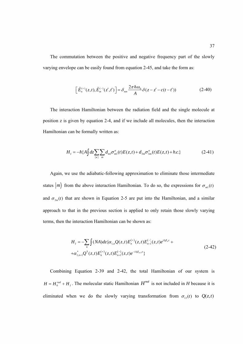
From a numerical evaluation of equation 2-52, there exists a dominant pair of
temporal modes of the Stokes field and a spatial mode of collective molecular coherence
if dispersion is absent. In Figure 2.8 we show the calculated photon number distribution

42
of most occupied temporal modes [42] in the generated Stokes field under different
dispersion conditions. The calculation assumes the Gaussian-shaped pump pulse and the
collisional dephasing was neglected. It shows that if there is no group-velocity difference
between Stokes and pump fields ( 0 0 ), the most occupied Stokes temporal mode has
a thousand times more photons than the second most occupied mode.
This existence of a dominant mode justifies that the generated Stokes field and the
collective molecular coherence can be simply treated in a two-mode squeezing state.
Generally, this state is also an entangled state, in analogy to an optical parametric down-
conversion process. The common explanation of this entanglement is, if one Stokes
photon is detected in output, then there must be a molecule also being transferred to its
excited state.
If there are many sidebands other than a single Stokes line in the comb generation,
then the above argument of entanglement is no longer rigorously valid. But since the
sidebands and molecular collective coherence are generated cooperatively, we conjecture
that they will be generated in a multi-partite entangled state.
43
Quantum entanglement between two atomic ensembles
In this section, I would like to briefly review one project that I had worked on before I
shifted my research focus to Raman frequency comb generation. This project utilized the
entanglement idea in a stimulated Raman scattering process, and was aiming to create an
entangled state between two distant objects, which are alkali atom ensembles. We used
atoms instead of molecules because the electronic Raman scattering in atoms has a much
Figure 2.8. Photon occupation number (equation 2.52) for different output modes
under different dispersion conditions: 0 0 (black bar), -10 ps/mm (gray bar)
and -30 ps/mm (hollow bar). Results are from reference [42].

44
longer lifetime, typically in the order of micro-seconds. This long quantum lifetime of
collective electronic spin (CES) coherence has played an important role in recent
quantum network experiments.
The entanglement scheme is plotted in Figure 2.9. The Stokes field generated by the
stimulated Raman scattering process in each atomic ensemble (A or B) was mixed at a
50/50 beamsplitter. The two outputs of the beamsplitter were then detected individually
by certain methods. After the measurement, the state of two atomic ensembles may be
collapsed into an entangled state, depending on the detection scheme.
In a spontaneous regime, where only very few Stokes photons were generated from
each ensemble, one can use avalanched photon detectors (APD) to simultaneously
measure whether there were photons or not in the output channels of the beam-splitter. In
any stance where only the upper channel detects one click, but the down channel detects
no photons, the state of the two atomic ensembles can be shown to be:
Figure 2.9. Scheme to generate entanglement between two atomic ensembles
45
1 0 0 1A B A B
(2-53)
This state is one of the maximum entangled Bell states [43].
If the Raman scattering in each ensemble was in a mesoscopic regime, which means
the Stokes photon number is in the range of 10 to 100, but still does not reach the
stimulated regime, the photon number-resolving detector can be used to measure how
many photons are in each output channel of the beamsplitter. If n and m photons were
detected, the resultant state of the two atomic ensembles is:
,1 2 ,
,1 2
1(tanh ) (tanh )
cosh coshi j n m
i j A Bi j
B i j
(2-54)
where ,,n mi jB is the beamsplitter transform matrix with a probability that a 50/50 beam-
splitter has i and j photons in its outputs if n and m photons are two inputs.
This state is not as easily verified as an entangled state, especially in an experiment.
One practical way to do it is to use a so-called “entanglement witness,” which is derived
from the Shchukin-Vogel scheme [44]. It measures various moments of creation and
annihilation operators of the beam-splitter’s two output channels jointly. In principle, this
type of measurement can be done by using a balanced homodyne correlation. A detailed
description of the proposed experiment can be found in [45].
If the Raman scattering in each atomic ensemble is in a stimulated regime, where the
Stokes field is generated at a macroscopic level, we can use balanced homodyne
detection to measure the quadrature operators in each output channel of the beamsplitter
[46]. Quadratures of Bosonic-like operators are defined as:
46
†1( )
2q a a
†1( )
2p a a
i
In order to generate entanglement, one measures the two output channels on an
orthogonal quantum basis. For example, if one measured the q quadrature in one output
of the beamsplitter, one would simultaneously measure the p quadrature in the other
output channel. If the measurement results from the above two joint measurements are Q
and P, respectively, then the state of the two atomic ensembles can be shown to be
collapsed to:
2 21 2
exp( 2 ) ,2 2
s vPq q i q Qq q q
s s
, (2-55)
where cosh , sinh , 2 2s and we assume two Raman scattering
processes have same gain coefficient 1 2 . ( ) / 2A Bq q q is the sum and
difference between the two q quadratures of the two atomic ensembles.
The state in Equation 2-68 can also be shown to be an entangled state. A detailed
analysis can be found in [47].
Another advantage of using Raman scattering to generate entanglement between two
distant atomic ensembles is that, by using a time-delayed control laser light, the quantum
state can be readout in an inverse process. This process is depicted in Figure 2-4, where
an anti-Stokes field is generated with all atoms in an excited state scattered back to

47
ground state. This allows the atomic ensemble to serve an important role as a memory
and information exchange node in a quantum network.

48
CHAPTER III
SPONTANEOUS PHASE CORRELATIONS IN RAMAN
OPTICAL FREQUENCY COMB GENERATION
Phase correlation between first order sidebands
Equations (2-46) and (2-47) in Chapter II that include all Raman sidebands is
extremely non-linear. There are no analytical solutions for those coupled non-linear
operator equations. However, as a simplifying case, we first consider the situation where
only first-order Stokes 1E and anti-Stokes 1E fields are created, and the pump intensity
profile is unchanged throughout the interaction. This simplified linear model allows us to
find a complete quantum description and gain insight into the comb generation process.
The coupled equations are:
( )1 2, 0
†( , ) ( ) ( , )z sE z i E Q z
( )1 2, 0
†( , ) ( ) ( , ) exp( )z aE z i E Q z i z
( ) ( )1, 1 0 1, 1 0
† ( , ) ( , ) ( ) ( , ) ( ) exp( )s aQ z i E z E i E z E i z (3-1)

49
where 1 1 02 is the phase mismatch of wave-vectors. Here we treat the
Raman pump as a classical field, and it stays unchanged through the entire interaction.
These coupled equations in 3-1 were first solved in a full quantum context by Kilin [48],
who verified that a slight phase mismatch is needed to maximize the generation of Stokes
or anti-Stokes sideband, as seen in experiments [49]. More general solutions than those in
[48] are found here using the methods in [40]. Assuming that the pulses are long enough
that group-velocity effects are not important, the field operators at the end of the fiber (z
= L) and at local time / v gt z (where v g is the group velocity of the pump) are
found to be:
( )( )2, 11 2, 12 1, 11
0 0 ( )( ) 02, 21 2, 22 1, 11
2, 130 0
( ; , ) ( ; , ) (0, ')( , )( ) ( )
( ; , ) ( ; , ) (0, ')( , )
( ; ,0) ( )
s s s
a a a
L s
G L G L EE LE d E
G L G L EE L
i G zE dz
( )1
( )2, 23 1
† (0, )( ',0)
( ; ,0) (0, ) i La
EQ L z
i G z E e
(3-2-1)
( ) ( )1, 0 13 1 1, 0 13 10
00
†
( , ) ( ) ( ; , ) (0, ) ( ) ( ; , ) (0, )
( ; ,0) ( ,0)
s a
L
Q L i d E G L E E G L E
dz G z Q L z
†
(3-2-2)
The Green propagators are given by:
11 12 120( ; , ) ( ; , ) ( ; , );
zG z G z i dz G z
22 12 12( ; , ) ( ; , ) exp( ) ( ; , );G z G z i i z G z
12 21 0 0( ; , ) ( ; , ) (2 ( , ) ) [ (2 ( , ) ) exp( )];s aG z G z I z J z i z
13 0 1( ; , ) (2 ( , ) ) [ ( ) (2 ( , ) ) ( , ) / exp( )];s a aG z I z z J z z i z
23 1 0( ; , ) [ (2 ( , ) ) ( , ) / ( )] [ (2 ( , ) ) exp( )];s s aG z I z z z J z i z

50
0 1
1
( ; , ) [ (2 ( , ) ) ( , ) / ( )]
[ ( ) (2 ( , ) ) ( , ) / exp( )]
s s
a a
G z I z z z
z J z z i z
where “*” denotes convolution on the variable z, and ,n nJ I are n-th order Bessel and
modified Bessel functions, respectively. The time-dependent gain coefficients are:
2
, 1,( , ) 2,( , ) 0( , ) ( )s a s a s a dt E t
. (3-3)
With the sideband fields initially in the vacuum state and all molecules in their
lowest-energy states 1 , the initial operators have the following correlation functions :
† ( ,0) ( ,0) (1/ ) ( )Q z Q z AN z z
†( ,0) ( ,0) 0Q z Q z
( ) ( )(0, ) (0, ) (2 / ) ( )n n nE E Ac
( ) ( )(0, ) (0, ) 0, 1n nE E n (3-4)
Equation (3-2-1) represents two types of processes: The terms coupling ( )1E
( ( )1E
)
with Q represent Stokes (anti-Stokes) scattering from ground-state (excited-state)
molecules. The off-diagonal terms in the green matrix coupling ( )1E with ( )
1E represent
Stokes/anti-Stokes four-wave mixing, in which two pump photons are annihilated and a
Stokes/anti-Stokes photon pair are created. Both of these processes drive the same
collective molecular excitation Q. The phases of the initiating vacuum (zero-point) fields
are temporally and spatially fluctuating, as shown in the delta correlation functions of

51
equation (3-4), which represents white noise in time and space. We could attribute this
fluctuation to a thermal-like field distribution of the temporal-spatial modes (TSM) of the
spontaneously emitted Stokes field, or equivalently to the thermal-like distribution of
longitudinal spatial modes of the collective molecular excitation [47, 50]. The laser field
further scatters from the collective molecular excitation creating additional anti-Stokes
light. Subsequently, the initial white noise is heavily filtered under the high-gain transient
conditions, since the gain process is a resonant one, and the Green propagators grow
exponentially as the pulse propagates through the medium. The filtering or smoothing
process eventually produces a Stokes and anti-Stokes field that are determined solely by a
single TSM each; in other words, each has the form of a smooth, transform-limited wave
packet with an overall phase and a peak amplitude that are random from one pump pulse
to another. In this sense, these two fields resemble classical fields, that is, complex
temporal envelopes with well defined carrier frequencies, although the intensities and
phases of both fields dramatically fluctuate from one shot to another [21, 47, 51]. It is
further known that if the scattering process goes into saturation, then the magnitude of the
intensity fluctuations greatly decreases [52], although this is not accounted for in the
linear theory considered here.
Next we examine the mutual coherence between generated first-order Stokes and
anti-Stokes fields, in the high-gain transient regime. We calculate the correlation
coefficient defined as
2( ) ( )1 1
( ) ( ) ( ) ( )1 1 1 1
( , ) ( , )
( , ) ( , ) ( , ) ( , )
E L E LC
E L E L E L E L
(3.5)

52
Because both fields in the numerator are negative-frequency ones, this gives the
degree of phase anti-correlation between generated Stokes and anti-Stokes fields. Writing
( ) ( )1 1 1I E E , the phase correlation coefficient is proportional to the degree of mutual
phase coherence, defined as 1 1( )iC e
, as is seen from:
1 1
2( ) ( )
21 1 ( )
1 1
iE E
C eI I
, (3-6)
if we assume that the fluctuations in intensities E1( )
2 of first-order Stokes and anti-
Stokes are independent of that of their phases. For example, if the temporal phase of the
Stokes pulse is statistically independent of the anti-Stokes pulse, the C value (and C )
would be zero. Also, if the two fields' phases tend to be equal, then C would be zero. In
contrast, if the sum of the phases of these two pulses stays constant from shot to shot
(while they both fluctuate), which indicates phase anti-correlation, then C would equal
one, and C would be determined by intensity fluctuations alone.
By putting expressions from (3-2) into equation (3-6) and using the initial conditions
(3-4), we calculate the C values under various conditions. The full expression is given in
the Appendix A, as well as in our publication [53]. In Figure 3.1 we plot C values and
Stokes and anti-Stokes intensities as functions of local time τ under the phase mismatch
condition 10L , where the anti-Stokes intensity is maximized (see Figure 3.2). In
all our calculations here we use 12 ns (FWHM) transform-limited Gaussian pump pulses,

53
and the Stokes and anti-Stokes integrated gain coefficients (2
1, 2, 0 ( )s s dt E t L
) are set
at the values of 25 and 30, respectively.
We see in Figure 3.1 that the value of C nearly equals 1 throughout the duration of the
generated Stokes pulses. Also note that the peak of the Stokes field is delayed by 4 ns
relative to the peak of pump field, which is consistent with previously known results [27].
In Figure 3.2 we show the calculated C value at the peak of the Stokes-pulse intensity
under various dispersion conditions, and find that its value stays close to 1. There we also
Figure 3.1. Pump and first-order Stokes and anti-Stokes mean
intensities and their anti-correlation C as functions of local time.

54
show the peak Stokes and anti-Stokes-pulse intensities versus phase mismatch, showing
the well-known minimum that occurs for perfect phase matching [48, 49,54].
The result 1C implies that the first-order Stokes and anti-Stokes are correlated in
the following way:
( ) ( )1 1E E
, (3-7)
where is a complex constant (with magnitude smaller than unity). This relation shows
that, not only the intensities of the two sidebands fluctuate in the same manner from pulse
Figure 3.2. First-order Stokes and anti-Stokes mean intensities, and
their anti-correlation C as functions of phase mismatch.
55
to pulse, but their phases are near perfectly anti-correlated. This confirms one of our
conjectures in [55]. It indicates a tendency in this system to automatically evolve toward
perfect phase anti-correlation, although our experimental observations show that the anti-
correlation is not perfect. A more rigorous model including all comb lines and pump
depletion is needed for explaining this discrepancy.
The generated sideband fields are also correlated with the collective molecular
excitation created in the medium, as seen in the solution (3-2-2). The quantity
( )1( , ) ( , )Q L E L , which is a measure of this field-medium correlation, is plotted in
Figure 3.3 as a function of the local time . It shows a maximum in time, following the
Stokes fields (see Figure 3.2). This correlation between field and molecular coherence
has been studied in experiment for the case that Stokes only was generated [50]. In the
absence of dephasing processes, this non-zero correlation can be considered as a
manifestation of quantum state entanglement between the medium and the fields.
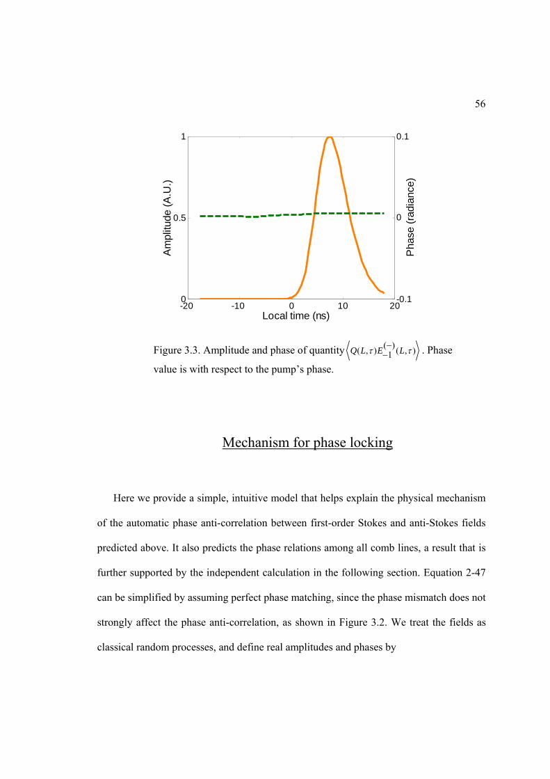
56
Mechanism for phase locking
Here we provide a simple, intuitive model that helps explain the physical mechanism
of the automatic phase anti-correlation between first-order Stokes and anti-Stokes fields
predicted above. It also predicts the phase relations among all comb lines, a result that is
further supported by the independent calculation in the following section. Equation 2-47
can be simplified by assuming perfect phase matching, since the phase mismatch does not
strongly affect the phase anti-correlation, as shown in Figure 3.2. We treat the fields as
classical random processes, and define real amplitudes and phases by
Figure 3.3. Amplitude and phase of quantity ( )( , ) ( , )1Q L E L
. Phase
value is with respect to the pump’s phase.
-20 -10 0 10 200
0.5
1
Local time (ns)
Am
plitu
de (
A.U
.)
Pha
se (
radi
ance
)
0
0.1
-0.1

57
( ) ( ) ; ni in nE E e Q Q e . (3-8)
This gives the evolution of the molecular polarization as:
1( ) ( )1, 1
n n
Ni
n n nn N
i Q Q E E e
, (3-9)
where we expressed the complex coefficient 1,ni in terms of an amplitude and phase:
1, 1, ( )n ni exp i . This gives two real equations:
( ) ( )1, 1 1cos
N
n n n n nn N
Q E E
( ) ( )1, 1 1
1sin
N
n n n n nn N
E EQ
(3-10)
The first equation in (3-10) implies that the molecular polarization grows at a
maximal positive rate if 1 0n n . In this situation, the second equation
implies that the random phase of the molecular polarization becomes time-
independent, as the sin function goes to zero. This result is consistent with the established
phenomenon of high-gain temporal filtering [50]. The idea is that the spontaneously
generated comb lines can arise with any phase values, and the values that actually occur
will be those leading to the highest overall gain, as indicated by the highest growth rate of
Q . This highest gain also leads to time-independent phases with particular relations
58
among them. This is similar to self-mode locking in a laser. For compactness, this
relation can be written as:
1n n , (3-11)
where absorbs the constant into the random phase . The random variable
has uniform probability between 0 and 2 [51]. For the case of a strong pump in the n
= 0 mode with phase 0 , this relation implies for the anti-Stokes and Stokes phases,
1 0 and 1 0 . These further imply perfect anti-correlation: 1 1 02 .
Now we can self-consistently solve for the phases of all comb lines from equation (3-
11), referenced to the pump phase 0 , giving
0n n . (3-12)
This simple relation, while meant only to indicate the ideal limit of perfect phase
locking (when phase mismatches are zero), is a useful guide in understanding the global
behavior of the system.
Semi-classical Raman modulator model
Because Equation 2-46 describing all the Raman sidebands is difficult to solve, and
the calculation in Section VI is only qualitative, we develop another supporting
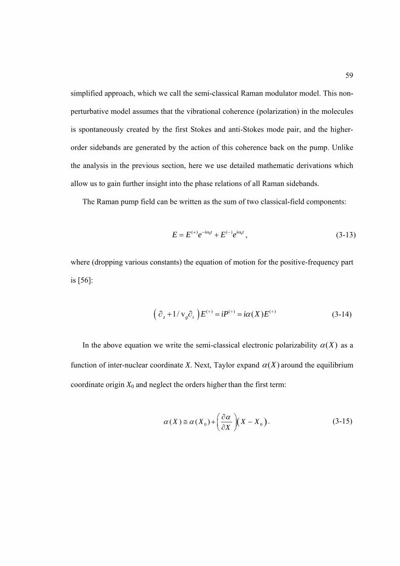
59
simplified approach, which we call the semi-classical Raman modulator model. This non-
perturbative model assumes that the vibrational coherence (polarization) in the molecules
is spontaneously created by the first Stokes and anti-Stokes mode pair, and the higher-
order sidebands are generated by the action of this coherence back on the pump. Unlike
the analysis in the previous section, here we use detailed mathematic derivations which
allow us to gain further insight into the phase relations of all Raman sidebands.
The Raman pump field can be written as the sum of two classical-field components:
0 0( ) ( )i t i tE E e E e , (3-13)
where (dropping various constants) the equation of motion for the positive-frequency part
is [56]:
( ) ( ) ( )1/ v ( )z g t E iP i X E (3-14)
In the above equation we write the semi-classical electronic polarizability ( )X as a
function of inter-nuclear coordinate X. Next, Taylor expand ( )X around the equilibrium
coordinate origin X0 and neglect the orders higher than the first term:
0 0( ) ( )X X X X
X
. (3-15)

60
We discard the α(X0) term, as it affects only the phase velocity of the electric field.
We also ignore for now any phase velocity mismatching in this model. By changing to
local time variable / v gz t z , equation (17) can be written as:
( ) ( )'z E i X E , (3-16)
where 'X
.
The electric field at the end of the Raman medium (z = L) can be obtained by
integrating the above equation:
( ) ( )
0
( , ) (0, )exp ' ( , )L
E L t E t i dz X z t
(3-17)
The X variable is related to the molecular polarization P created in the medium by [56]
13
13
†( , ) ( , ) . .
2 ( , ) cos ( , )
i tX z t P z t e h c
p z t t z t
, (3-18)
where 13 is the molecular resonance frequency, and ( , )z t is the random phase variable
arising from the Raman process. By putting equation (3-18) into equation (3-17), we get

61
( )
( )
0
( )
( , )
(0, ) exp ' 2 ( , ) cos ( , )
(0, )exp ( ) cos ( )
L
R
R
E L t
E t i dz p z t t z t
E t i a t t t
(3-19)
where ( ) ( , )
0( ) 2 ' ( , )
Li t i z ta t e dz p z t e . We use a mathematical expansion for the
phase part of the above equation, i.e., exp( cos( )) ( ) expnn
n
i x i J x i n
, and we
use ( ) ( 1) ( )nn nJ x J x to re-write ( ) ( 1) ( )n
n nJ x J x . Then
( )
( )
( )
( , )
(0, ) ( ) ( ( ) ) exp ( ( ))
(0, ) ( ( ) )exp ( ( ) / 2)
nRn
n
Rnn
E L t
E t i J a t in t t
E t J a t in t t
(3-20)
If we write ( ) ( ) / 2t t , then
( )
( )
( , )
(0, ) ( ( ) )exp ( ) exp Rnn
E L t
E t J a t i n t i n t
(3-21)
We can identify the complex amplitudes of the Stokes and anti-Stokes lines as:
( ) ( )( , ) (0, ) ( ( ) )exp ( )n nE L t E t J a t in t

62
We see that the first-order Stokes (n = 1) and anti-Stokes (n = –1) fields are predicted
to have opposite phases, which is the same conclusion we derived earlier from the more
rigorous quantum theory for the case of only two side bands. Equation 3-21 is similar to
the one derived in reference [35], except that here only a single pump is used and the
effects of quantum fluctuations (ignored in [35]) are paramount. More interestingly,
equation 3-21 predicts that the higher orders of Stokes and anti-Stokes fields will have
their temporal phases related to the phase of the strong pump ( 0 ) by:
0 ( )n n t . (3-22)
Under high-gain transient conditions, the phase ( )t will be essentially constant
during a single pulse, as discussed above. Therefore, this prediction is the same as
obtained in equation (3-12) using a distinct and more qualitative argument. It can be
understood, since higher-order sidebands arise from multiple scattering from the Raman
medium. Each time the field gets scattered, the Raman medium will impose a phase
shift onto it.
Prospects for ultrashort pulse generation
Combining the ideal relation (3-22) with the frequency relations (2-2), we find that
the generated comb spontaneously satisfies the required relations for Fourier synthesis to
create a periodic waveform. In order to see that, express the synthesized waveform as:
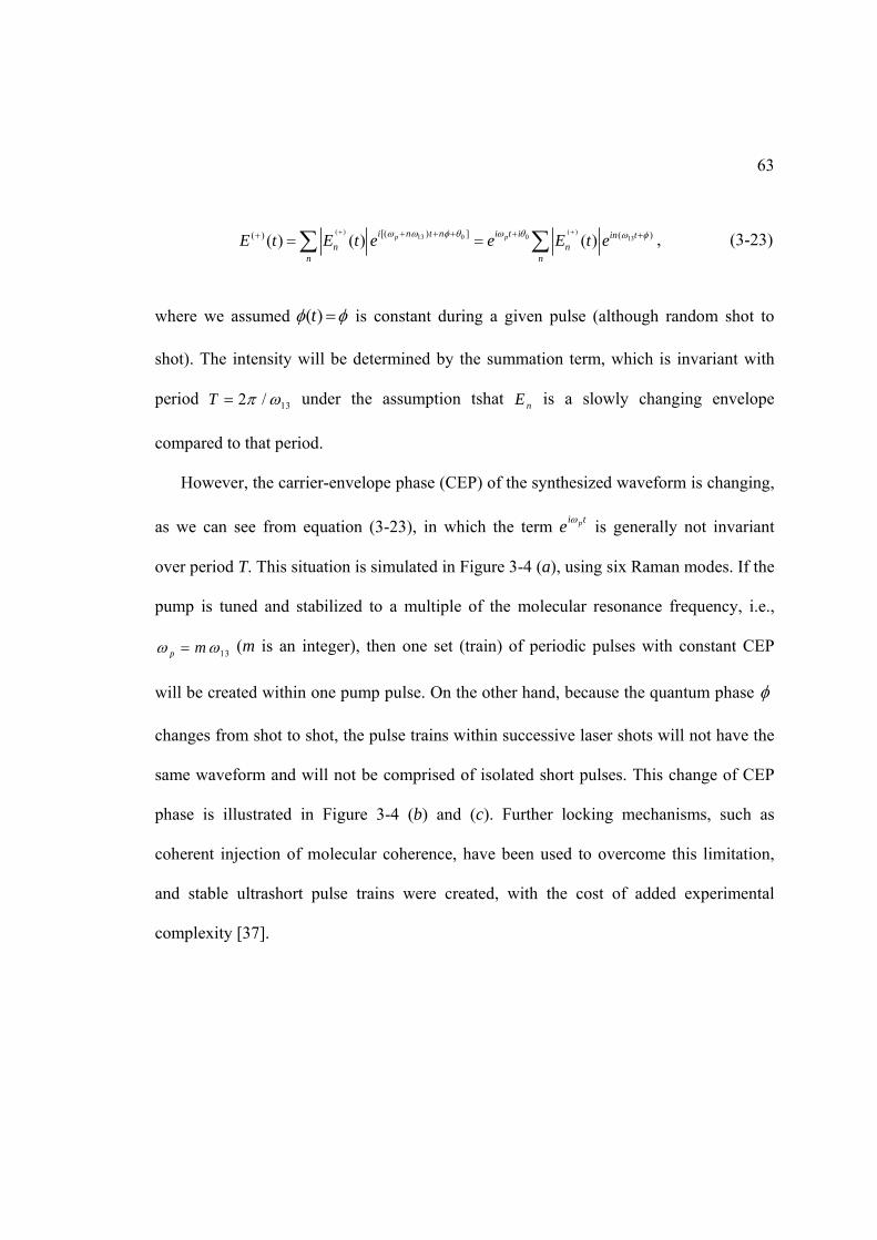
63
( ) ( )13 0 0 13
[( ) ] ( )( ) ( ) ( ) ( )p pi n t n i t i in tn n
n n
E t E t e e E t e , (3-23)
where we assumed ( )t is constant during a given pulse (although random shot to
shot). The intensity will be determined by the summation term, which is invariant with
period 132 /T under the assumption tshat nE is a slowly changing envelope
compared to that period.
However, the carrier-envelope phase (CEP) of the synthesized waveform is changing,
as we can see from equation (3-23), in which the term pi te is generally not invariant
over period T. This situation is simulated in Figure 3-4 (a), using six Raman modes. If the
pump is tuned and stabilized to a multiple of the molecular resonance frequency, i.e.,
13p m (m is an integer), then one set (train) of periodic pulses with constant CEP
will be created within one pump pulse. On the other hand, because the quantum phase
changes from shot to shot, the pulse trains within successive laser shots will not have the
same waveform and will not be comprised of isolated short pulses. This change of CEP
phase is illustrated in Figure 3-4 (b) and (c). Further locking mechanisms, such as
coherent injection of molecular coherence, have been used to overcome this limitation,
and stable ultrashort pulse trains were created, with the cost of added experimental
complexity [37].

64
We are presently exploring whether simultaneous pumping of the medium by a
fundamental pump and its phase-locked second harmonic, as in [37], but without external
injection of coherence, can also lead to stable ultrashort pulse trains by a generalization
of the phase locking discussed in the present Chapter. If the frequency of the fundamental
pump is tuned to be precisely an integer multiple of the molecular resonance frequency,
the frequency-doubled pump will be resonant with one of the anti-Stokes fields of the
Figure 3.4. Simulated short pulses under different conditions. a) 13p m . b)
13 , 0p m . c) 13 , / 6p m . From (b) and (c) it clearly shows the
change of carrier-envelope phase in the synthesized pulses.
(a)
(b) (c)

65
original pump. For example, if we choose hydrogen molecules as our Raman medium,
the vibrational resonance frequency is around 125 THz [39]. We can tune the pump to
about 375 THz (or 802 nm), which is in the range of commonly used Ti-sapphire lasers.
The frequency-doubled pump (401 nm) will be resonant with the third anti-Stokes field
of the original pump, and will have a deterministic temporal phase relative to the
pump. Both the pump and its frequency-doubled beam will simultaneously interact with
hydrogen molecules to generate the comb. The question is whether this will
deterministically lock the temporal phase difference among adjacent comb lines, which is
in equation (3-22), to the value / 3 , the only value that allows a self-consistent
phase anti-correlation between all comb lines. The produced periodic single-cycle pulse
trains will then be identical upon subsequent pump pulses.
66
CHAPTER IV
OPTICAL RAMAN COMB GENERATION
Hollow-core Photonic Crystal Fiber
The hollow-core photonic crystal fibers (HCPCF) that we used in our experiments
were fabricated by and generously provided by Dr. Fetah Benabid and his research group
at the University of Bath in the UK. HCPCF consists of a large air hole in the “core” area,
and a periodic 2-D crystal structure-like lattice as the fiber’s cladding. By using HCPCF,
we can fill it with Raman active gases, such as hydrogen or CH4, at various pressures.
Also, HCPCF has shown broadband transmission from ultra-violet to infrared. This
multiple octave span in wavelength will be greatly useful in generating the optical Raman
frequency comb that is wide enough for the atto-second pulse to synthesize.
Although I do not make the HCPCF myself, I would like to briefly describe the
process involved in making it [57, 58], which has the following three-stage drawing: In
the first step, a hexagonal unit cell on a macroscopic scale is formed by drilling a hole
down the length of a silica rod. In a typical photonic crystal fabrication process, the
diameters of the hole and the rod are 16 mm and 30 mm, respectively [57]. Six flats are
67
then milled on the outside of the rod, forming a regular hexagon. In the second step, the
preform of a hexagonal unit cell is drawn on a fiber drawing tower at a certain
temperature and pressure to produce hexagonal cane of a diameter at the order of 1mm,
which is cut to short lengths and stacked to give the required crystal structure. This
hexagonal cane of a small diameter is usually called a “thin capillary.” In the third step,
the stack of capillaries forming a certain crystal structure is again drawn on the tower,
fusing the stacked canes together and reducing the pitch (center-to-center spacing) to a
certain small value. Finally, a piece of this fused stack is drawn down again to yield the
final fiber.
The crystal structure of the HCPCF that we got and used in our experiment from the
University of Bath is called a Kagome structure, and it has a large hole (about 20 microns)
in the center. The fabrication technique to introducing such a core defect is applied in the
second step, where shorter capillaries are stacked on both sides of the capillary, leaving a
gap in the middle. During the cane-pulling process (the third step), no cladding or core
pressurization is applied. The drawing temperature is kept low in order to form the
Kagome structure. During the fiber-drawing process (the final step), the integrity of the
structure is preserved by independently pressurizing the core, the cladding, and the region
separating the jacket tube from the cane. Moreover, to maintain the structure’s air-filling
fraction, the Kagome fiber is drawn at a low temperature, high-preform feed rate, and
high drawing tension. Figure 4.1 shows the scanning electron microscope of the
transverse structure of the Kagome fiber, after the fiber has been cleanly stripped and
cleaved.
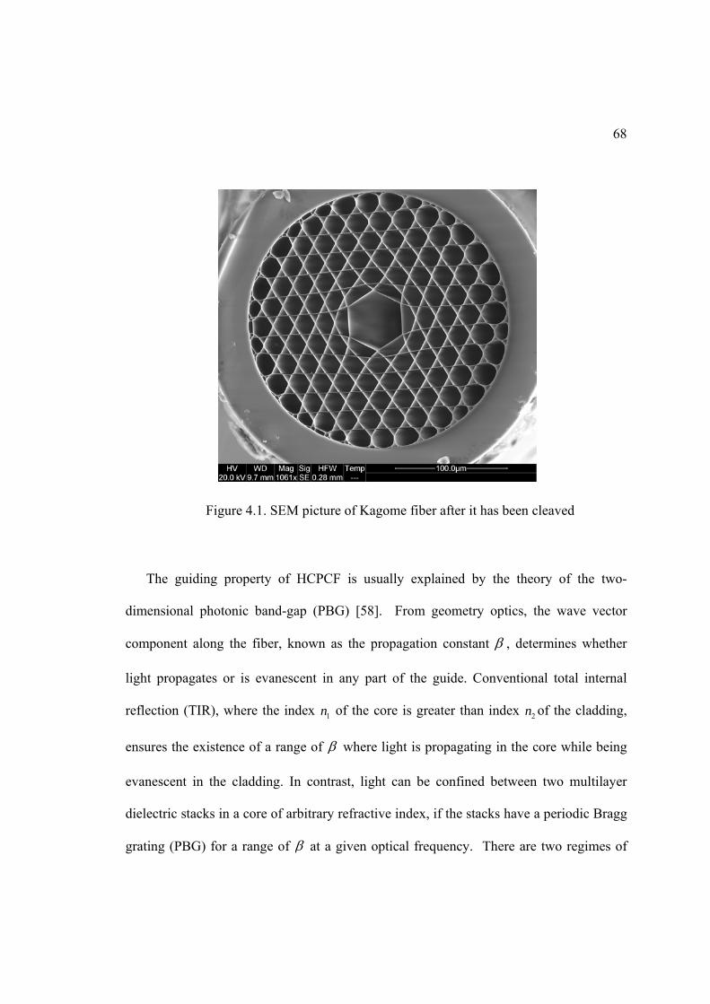
68
The guiding property of HCPCF is usually explained by the theory of the two-
dimensional photonic band-gap (PBG) [58]. From geometry optics, the wave vector
component along the fiber, known as the propagation constant , determines whether
light propagates or is evanescent in any part of the guide. Conventional total internal
reflection (TIR), where the index 1n of the core is greater than index 2n of the cladding,
ensures the existence of a range of where light is propagating in the core while being
evanescent in the cladding. In contrast, light can be confined between two multilayer
dielectric stacks in a core of arbitrary refractive index, if the stacks have a periodic Bragg
grating (PBG) for a range of at a given optical frequency. There are two regimes of
Figure 4.1. SEM picture of Kagome fiber after it has been cleaved

69
PBG guidance. In the first regime, light propagates in the layers with high index 1n of the
dielectric stack but is evanescent in the layers with low index 2n . The high-index layers
act as individual TIR waveguides, supporting bound modes at specific values of m .
Resonant tunneling between adjacent high index layers permits the leakage of light
through them, provided lies within the pass bands that open up around each m . The
widths of the pass bands depend on the strength of coupling between the layers. Between
the pass bands lie band gaps; if a high-index core layer with a different (maybe smaller)
width supports a mode with inside a band gap, it is not resonant with the other layers
and light leakage by tunneling is frustrated. The mode is thus strictly guided by the
frustrated tunneling form of PBG. In the second regime of PBG guidance, light can
propagate in all layers ( 2k n ). Band gaps occur at the Bragg condition as a result of
multiple scattering and interference, leading to the Bragg form of PBG guidance.
The Kagome fiber, although it belongs to HCPCF, relies on a new photonic guidance
whereby photons are confined not by PBG but rather via a mechanism akin to Von
Neumann-Wigner bound states [59, 60] within continuum, where the fiber-guided modes
cohabitate with those of the cladding without notably interacting. This “inhabited
interaction” between the hollow core-guided modes and the cladding continuum is
explained by the high degree of the transverse-field mismatch between the core and
cladding modes [39].
The guiding property of a Kagome fiber is mainly determined by its pitch (Λ), core
size, strut width and air-filling fraction. The fiber that we used in the experiment and will
discuss throughout this chapter has a single core air hole with a diameter of 20 microns
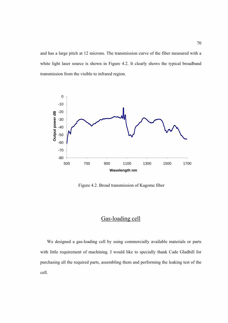
70
and has a large pitch at 12 microns. The transmission curve of the fiber measured with a
white light laser source is shown in Figure 4.2. It clearly shows the typical broadband
transmission from the visible to infrared region.
Gas-loading cell
We designed a gas-loading cell by using commercially available materials or parts
with little requirement of machining. I would like to specially thank Cade Gladhill for
purchasing all the required parts, assembling them and performing the leaking test of the
cell.
Figure 4.2. Broad transmission of Kagome fiber
-80
-70
-60
-50
-40
-30
-20
-10
0
500 700 900 1100 1300 1500 1700
Ou
tpu
t p
ow
er
dB
Wavelength nm

71
Figure 4.3 shows the detailed drawing of the cell. The main part of the cell is a 3/8”
female pipe thread tee. The input end is connected with another pipe thread tee where a
hydrogen gas tank and a pressure gauge are attached. One output of the female pipe
thread tee is connected with a pipe-thread (3/8”) to a VCO (1/2”) adapter. A 3 mm thick
optical window (BK7) is put inside a VCO-type nut, and this output end is sealed by
capping the nut, which essentially pushes the window firmly against the o-ring that is
built inside the VCO adapter. In the other output end, where fiber will be loaded, a 1/8”
Swagelok straight fitting to a 3/8” pipe thread is directly attached. In order to seal this
end, a graphite ferrule with a .5 mm OD capillary is used. When loading the fiber into the
cell, one first inserts the un-cleaved fiber through the Swagelok nut, and then through the
ferrule carefully. Next insert the fiber into the Swagelok fitting that is already attached to
the pipe thread tee, and push the fiber through the pipe until it hits a plastic fiber guide
placed inside the VCO adapter. This fiber guide is the only self-machining part in the
design of this gas-loading cell. It has a center hole that is large enough to allow fibers to
go through. The purpose of this fiber guide is to support the fiber against its gravity.
Several small holes are drilled around the center hole in the fiber guide so that gas can
still be filled with the whole pipe thread tee. Special care should be taken so that the fiber
is inserted through the center hole of the fiber guide, instead of the small holes around it.
After the fiber end appears on the other end (window is not put on at this time), carefully
thread the Swagelok nut with the ferrule placed inside. This end should stay loose, so that
the fiber still can be pulled from the other end and then cleaved. After cleaving, pull the
fiber end back through the cell until its tip is inside the VCO fitting but outside the fiber
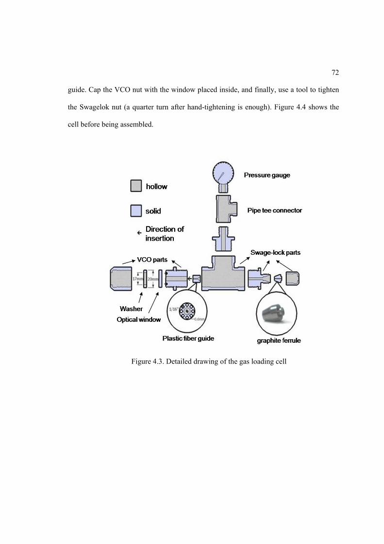
72
guide. Cap the VCO nut with the window placed inside, and finally, use a tool to tighten
the Swagelok nut (a quarter turn after hand-tightening is enough). Figure 4.4 shows the
cell before being assembled.
Figure 4.3. Detailed drawing of the gas loading cell
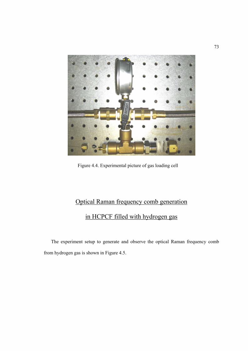
73
Optical Raman frequency comb generation
in HCPCF filled with hydrogen gas
The experiment setup to generate and observe the optical Raman frequency comb
from hydrogen gas is shown in Figure 4.5.
Figure 4.4. Experimental picture of gas loading cell

74
The light source we use is from a mode-locked Ti:Sappire laser (Spectra-Physics,
Tsunami) pumped by CW diode-pumped laser (Spectra-Physics, Millennium Pro) at 532
nm. The laser produces near 200 pico-second (ps) pulses at 80 MHz repetition rate. The
output pulse of the laser is monitored by two pieces of equipment: one is an ultra-high-
resolution wave-meter (Burleigh 1600) and another one is a high-speed photo-detector
(25GHz, New Focus 1437). The wave-meter displays the center wavelength of the pulse
to the accuracy of 10-4 nm (calibrated by Rubidium 87 D1 transition). The fast photo-
diode measures the temporal shape of the pulse, and ensures that the Ti:Sapphire laser is
Figure 4.5. Experiment setup for observation of Raman optical frequency comb
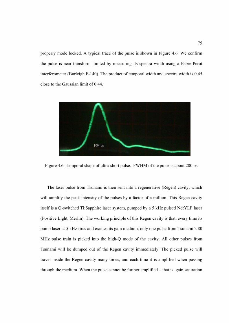
75
properly mode locked. A typical trace of the pulse is shown in Figure 4.6. We confirm
the pulse is near transform limited by measuring its spectra width using a Fabre-Perot
interferometer (Burleigh F-140). The product of temporal width and spectra width is 0.45,
close to the Gaussian limit of 0.44.
The laser pulse from Tsunami is then sent into a regenerative (Regen) cavity, which
will amplify the peak intensity of the pulses by a factor of a million. This Regen cavity
itself is a Q-switched Ti:Sapphire laser system, pumped by a 5 kHz pulsed Nd:YLF laser
(Positive Light, Merlin). The working principle of this Regen cavity is that, every time its
pump laser at 5 kHz fires and excites its gain medium, only one pulse from Tsunami’s 80
MHz pulse train is picked into the high-Q mode of the cavity. All other pulses from
Tsunami will be dumped out of the Regen cavity immediately. The picked pulse will
travel inside the Regen cavity many times, and each time it is amplified when passing
through the medium. When the pulse cannot be further amplified – that is, gain saturation
Figure 4.6. Temporal shape of ultra-short pulse. FWHM of the pulse is about 200 ps
76
occurs – the cavity is switched to low-Q mode and thus the amplified pulse is ejected out
of the Regen cavity. A combination of an electro-optic modulator (EOM) and a thin-film
sheet polarizer inside the cavity is used as a Q-switcher to pick and eject the pulse. The
timing of EOM is precisely controlled by a four-channel digital delay generator (Stanford
Research DG535). The output of the Regen cavity is an intensified pulse with 160 micro-
joules per pulse at a 5 KHz repetition rate. Details of this Regen cavity configuration can
be found in [61].
The pulses from the Regen cavity first go through a half-waveplate and a polarizer so
that they are linearly polarized in a horizontal direction, and then collimated by a pair of
lenses (300 mm and 100 mm focal length, respectively). We use a 35-mm, anti-reflection
doublet aspheric lens (Edmond Optics) coated for near IR (700 nm -1100 nm) to couple
the light into the HCPCF. Usually the fiber length is about 1.5 meters. The output of the
fiber is then collimated by another doublet lens at 60 mm. An equilateral dispersive prism
is used to disperse the collimated output, whose spectrum is then projected onto a distant
screen for easy viewing.
In the experiment, we seal one fiber end with the home-designed hydrogen gas-
loading cell, and leave the other fiber end open. The hydrogen gas is then pressurized into
the loading cell, typically between 5 and 15 bars, and then diffused into the HCPCF.
Since the output end is open, we can imagine there are hydrogen molecules blowing out
from that end. However, since the fiber transverse area (<100 microns) is very small
compared to fiber length (typically at 1.5 meters), the flow rate of hydrogen gas is very
low. In the experiment, we never notice the hydrogen gas leaking from the open end.
77
The Raman frequency shift 13 of hydrogen gas has slight dependence on gas
pressure, and has been found in a previous experiment as [62]:
2 (GHz) 9.6 10 pressure (bar) .
When hydrogen gas is set at 15 bars, 13 is estimated to shift by 1.4 GHz from the
above equation. This shift is still smaller than our laser’s linewidth (2.2 GHz). We
normally just neglect the impact of this small shift in our later experiment.
The Raman optical frequency comb that we observed in our lab is shown in Figure
4.7. To generate such a spectrum, we put an extra quarter-wave plate before the pulses
are coupled into the HCPCF, so that the Raman pump pulses are circular polarized. The
spectrum shown then is the hydrogen rotational line, which has line separation at 18 THz.
In order to show the spectrum, we use a standard digital camera to record the picture of
the spectrum scattered off the screen. The figure shows many high-order anti-Stokes lines
in the deep blue region, but fewer Stokes lines. This is because the Stokes lines are in an
infrared region, and the camera has poor or no response in this spectral region. We
estimate the pulse intensity required to generate such a spectrum is about a 5-10 µJ /
pulse, when the gas cell is kept at the pressure of 200 PSI. This required pump intensity is
much lower than the 1 mJ / pulse that is usually required in free-space setups.

78
In our later experiment, we take out the extra quarter-wave plate and couple the
linearly polarized pump pulses into HCPCF, which will excite the molecular vibrational
state in hydrogen gas. The frequency shift in this case is very large, about 125 THz. In
Figure 4.8, it shows the comb that we observe on the screen. In order to illustrate the
first-order Stokes at a wavelength of 1200 nm, we have used our IR viewer device, which
is responsive from 1100 nm to 1700 nm. The second-order Stokes, however, is at 2200
nm, and we cannot show it in the figure. For anti-Stokes fields, we observe up to 3 orders.
Their wavelengths are 602 nm, 488 nm and 401 nm, respectively. We label those Raman
comb lines with integer numbers, as we discussed in Chapter II. Stokes orders are
negative integers, and anti-Stokes orders are positive integers.
Another feature we can see from this Raman comb generation in gas-filled HCPCF is
that the output from the fiber after collimation shows a near Gaussian-like spatial mode
for almost every comb line, except those high-order anti-Stokes lines near the blue region.
This shows that the HCPCF helps to produce single spatial mode Stokes and anti-Stokes
in the comb. Since the effective cross-section of the HCPCF is only 20 microns, our
Figure 4.7. Hydrogen rotational comb
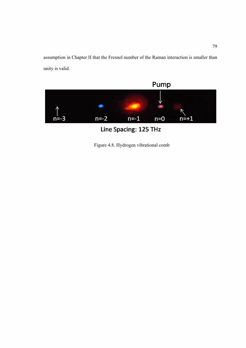
79
assumption in Chapter II that the Fresnel number of the Raman interaction is smaller than
unity is valid.
Figure 4.8. Hydrogen vibrational comb

80
CHAPTER V
EXPERIMENTS AND RESULTS OF PHASE
CORRELATION MEASUREMENT
Energy statistics of generated first-order Stokes field
The Raman optical frequency comb shown in the previous section is generated by
200 ps optical pulses. The interaction between the optical pulse and the hydrogen
molecules are in the so-called transient regime, where the molecular dephasing time 2T is
much longer than the pulse duration. Typically this 2T for hydrogen molecules are in the
order of 1 nanosecond. In reference [63], it is shown that transient regime can be satisfied
even when the pulse duration is longer than dephasing time 2T under ultra-high gain
condition. If the steady-state Raman gain is denoted as ssG , then for a pulse duration
shorter than 2ssG T , the interaction is said to be under transient regime.
In the experiment we measure the energy statistics of first-order Stokes (vibrational
line, wavelength at 1200 nm) to verify that our comb generation is under transient regime,
and also no photon at Stokes wavelength is seeding the process. In other words, the first-
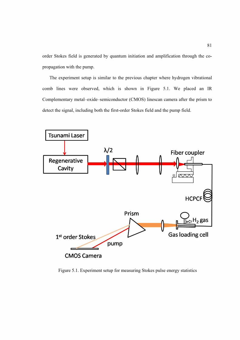
81
order Stokes field is generated by quantum initiation and amplification through the co-
propagation with the pump.
The experiment setup is similar to the previous chapter where hydrogen vibrational
comb lines were observed, which is shown in Figure 5.1. We placed an IR
Complementary metal–oxide–semiconductor (CMOS) linescan camera after the prism to
detect the signal, including both the first-order Stokes field and the pump field.
Figure 5.1. Experiment setup for measuring Stokes pulse energy statistics

82
This CMOS linescan camera was purchased from Photon Control, Inc. It consists of a
Hamamatsu InGaAs CMOS array detector and an electronic driver board that will allow
the detection under external triggering mode. The detector itself has 512 pixels, and each
pixel is 25 µm × 125 µm. Its spectral response is from 800 nm to 1650 nm. The detector
also has a very fast integration time, which can go down as small as 1 µs. We set the
detector at the external triggering mode, where the trigger signal is directly from the
pump laser. In this setup, once the detector received a low-to-high TTL signal, it will start
to integrate (count the photons hit on each pixel) for certain amount of time (integration
time), and then automatically shut down for some time (several milliseconds) to read out
the data on each pixel. This read-out process is usually called ‘binning.’ After it finishes
transferring data to the built-in memory, the detector will send a “data ready” signal to
the computer via the USB-connection cable. The computer will then read the data from
the detector’s memory and display it on the monitor. After reading the data, the computer
will signal the detector and the detector will clear its memory and zero any electrons that
are accumulated on each pixel during the blackout period, and wait for the next available
trigger signal to start its next operational cycle.
In this way, we can detect the dispersed single-shot first-order Stokes and pump field
if we set the detector’s integration time shorter than the time between consecutive pulses,
which is at about 200 µs. In the experiment, we set this integration time at 180 µs. The
frame rate of the camera is about 100 Hz, mainly limited by its data-binning and transfer
speed. The CMOS detector array is slightly different from the charge coupled device
(CCD) version, in that each pixel on the CMOS detector has its own amplifier, while all

83
pixels on CCD detector share one amplifier. Therefore, CMOS has a limitation on its
response linearity of all pixels. In our CMOS detector array, the specification of linearity
is better than 95%.
In Figure 5.2 we show the typical single-shot Stokes and pump signal recorded on the
CMOS linescan camera. We adjusted the beam height so that the array detector
(horizontal line) is centered across the beam. We also use neutral density filters to
attenuate the beam to prevent any saturation on the camera’s pixels. The beam sizes of
the first-order Stokes and pump are a little different shown from the data image. This is
because the numerical aperture of the HCPCF is not all the same for different colors of
light.
Figure 5.2. Single-shot first-order Stokes and pump signals

84
In the experiment, we keep the pump’s intensity low so that only the first-order
Stokes is present. No other comb lines can be observed by the eyes. In this way, we can
compare our measurement with previously known results for the stimulated Raman
scattering [21]. The histogram showing the probability distribution of the Stokes pulse
energies is plotted in Figure 5.3. In this figure, we analyze 300 total recorded camera
shots, and the peak value of the Stokes pulse in each shot is extracted to represent the
Stokes pulse energy. We can see that the histogram shows negative exponential
distribution for the Stokes pulse energy, i.e., the most probable Stokes energy is near zero.
This statistical feature of Stokes energy shows great fluctuations from one shot to another,
and is directly related to the vacuum initiation of the Stokes field. In quantum optics, the
exponential decay distribution is related to the Bose-Einstein distribution, where the
probability can be written as [64]:
1( )
(1 )(1 1/ )EP E
E E
.
In the above equation, E is the mean of Stokes pulse energy. The distribution peaks
at zero. However, when there is saturation, the above formula will no longer be valid.
That’s the main reason we kept our pump intensity low in our experiment.
However, it has also been shown that, even when 0E , the Stokes energy
distribution might deviate from a negative exponential to Gaussian. This is when the
generated Stokes pulse has several spatial and temporal modes (i.e. wave-packet modes).
Although each mode obeys a negative exponential distribution, the overall behavior of

85
Stokes energy statistics will then converge to a Gaussian distribution. An easy way to see
this effect is by using the analogy of the central limit theorem in classical probablity
theory. A detailed review on this topic can be found in [27]. Since our experiment shows
that the Stokes energy distribution is close to a negative exponential, the generated Stokes
field is in a single temporal and spatial mode. In other words, the Stokes field is close to
Fourier-transform limited pulse with a well-defined temporal phase. In the next section,
we will see that this temporal phase is also random from shot to shot due to the quantum
initiation process of the Stokes field.
In Figure 5.4 we also show the energy statistics of the pump laser. This plot is to
confirm that the large energy fluctuation of the Stokes field is not caused by the pump’s
Figure 5.3. Intensity statistics of first-order vibrational Stokes
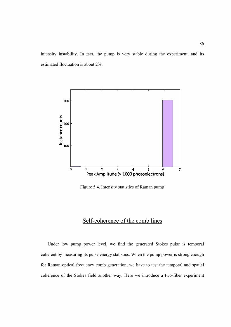
86
intensity instability. In fact, the pump is very stable during the experiment, and its
estimated fluctuation is about 2%.
Self-coherence of the comb lines
Under low pump power level, we find the generated Stokes pulse is temporal
coherent by measuring its pulse energy statistics. When the pump power is strong enough
for Raman optical frequency comb generation, we have to test the temporal and spatial
coherence of the Stokes field another way. Here we introduce a two-fiber experiment
Figure 5.4. Intensity statistics of Raman pump

87
where we interfere the same comb components generated independently from two fibers.
This technique was first used for Raman studies in "bulk" gas cells by Kuo et al [51]. The
high-visibility and random interference fringe phase indicate that the generated comb
lines are temporally coherent but have a random phase.
The experiment setup is shown in Figure 5.5. The pump pulse is again the output
from the Regen cavity with 200 ps temporal duration. It is split by a non-polarizing
beam-splitter (BS-A) into two parts, and each part is then coupled into a hydrogen-gas
filled, 1.5 meter-long HCPCF. The output of each HCPCF is then collimated by a pair of
lenses, which will ensure both outputs have similar beam diameters. These two beams are
combined by a small angle on a non-polarizing beam splitter (BS-B), and a narrow band
filter is placed in each output of the beam splitter to filter out single Stokes or anti-Stokes
line. A CCD or CMOS camera is placed afterwards to capture the interference fringes.
It is obvious that from BS-A to BS-B the alignment is a well-known Mach-Zander
interferometer. Each arm of this interferometer contains an HCPCF. In order to see
interference fringe on the camera, the distance of these two arms should be balanced, so
that the light pulses would overlap in the time domain.
Before the hydrogen gas is pumped into the HCPCF fiber, we test the balance of the
two arms by overlapping two pump beams transmitted from each fiber onto a non-linear
semiconductor photodetector. The intensity-squared dependence of the voltage signal
generated by the detector has a cross term depending on the two pump beams intensity
and their temporal overlap. This cross term is non-zero only when the temporal difference
between two pumps is smaller than the pump’s duration, and will be peaked when this

88
difference is perfectly zero. This cross-term signal is much more easily detected than
interference fringes, since it does not depend on the phases of two pumps. We place a
manually adjustable delay stage in one arm of the interferometer to fine-tune the distance
difference.
After we balanced the two arms of the interferometer by using an optical delay line,
we observed the interference fringes on the linescan detector. Mathematically, the fringe
can be expressed as:
Figure 5.5. Experiment setup for observation of interference
fringes from two Raman optical frequency combs. The dash-
dotted bracket indicates the two fiber interference setup.
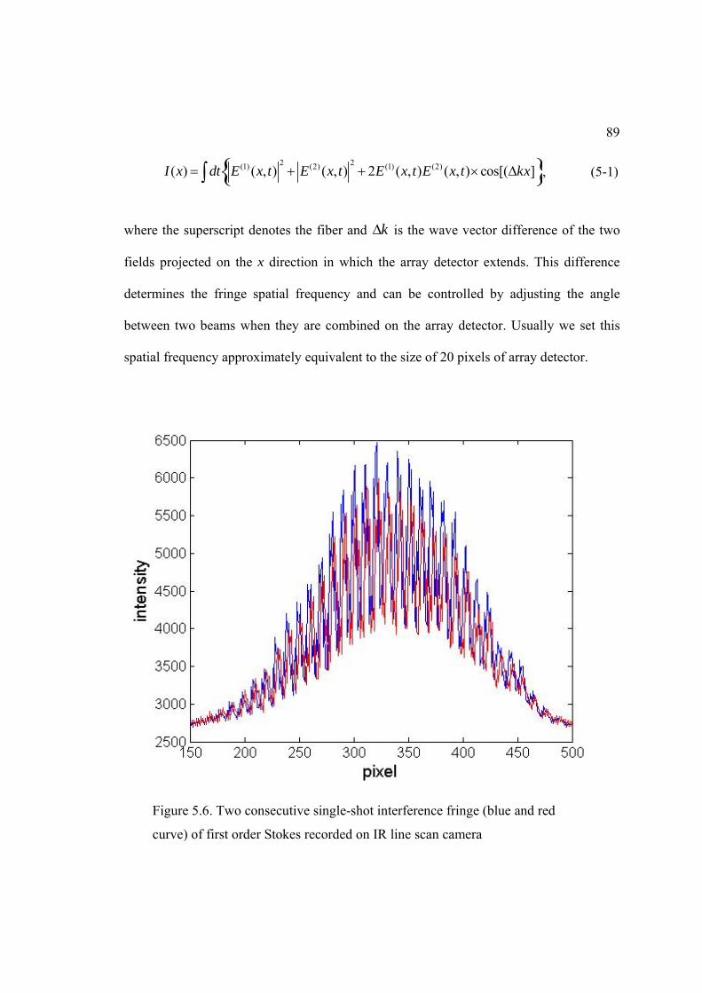
89
2 2(1) (2) (1) (2)( ) ( , ) ( , ) 2 ( , ) ( , ) cos[( ]I x dt E x t E x t E x t E x t kx , (5-1)
where the superscript denotes the fiber and k is the wave vector difference of the two
fields projected on the x direction in which the array detector extends. This difference
determines the fringe spatial frequency and can be controlled by adjusting the angle
between two beams when they are combined on the array detector. Usually we set this
spatial frequency approximately equivalent to the size of 20 pixels of array detector.
Figure 5.6. Two consecutive single-shot interference fringe (blue and red
curve) of first order Stokes recorded on IR line scan camera

90
In the experiment, we took extra care to keep the intensity of the two pumps that are
coupled into two HCPCF approximately equal, since the two fibers are not exactly same.
For example, their lengths, degrees of bending (which affects the loss of the fibers), and
their cleaving conditions are all slightly different. We balance these effects so that the
two generated first-order Stokes fields should approximately have same properties.
In figure 5.6 we show the two “consecutive” single-shot interference fringes of first-
order Stokes that we observed on the IR linescan camera. Here “consecutive” means two
successive camera shots (at about 100 Hz), instead of the laser shots (at 5 kHz). Since the
intensity of each Stokes field, like we show in previous section, is greatly fluctuating
from one shot to another, the visibility of the fringes is also fluctuating. The figure shows
a typical good fringe with an estimated visibility of 0.7. This high visibility reveals that
the first-order Stokes field is highly self-coherent, or in other words, the Stokes field is
temporal transform limited pulses, which is consistent with our conclusion in the
previous section. Another feature that we observed is that the fringes are randomly
moving from one shot to another. This movement is not due to the instability of the
interferometer, but is a direct result of the quantum-generated random phase of the first-
order Stokes field. From Equation 4-1, if we re-write the electric field of generated
Stokes as:
( ) ( )( , ) .j j
n n ni i t ik zj jnE x t E e e c c , (5-2)

91
where j (= A or B) indicates the fiber number, and n is -1 for the Stokes line, then the
spatial oscillation of the interference fringe is directly related to the difference of
temporal phases of two Stokes fields by:
1cos( )oscI kx . (5-3)
The movement of the interference fringes from one shot to another can come from
two factors, that is, the wave vector difference k and the phase difference 1 . The
parameter k is directly related to the stability of the two-fiber interferometer, and we
verify that this k is not changing from one shot to another because the interference
fringes from the two Raman pumps are very stable. In this sense, we determine that the
movement of the interference fringes indicates the temporal phase of the generated
Stokes field is random from shot to shot. If we set a reference (or zero) phase point in our
obtained interference fringe, we can get the phase value 1 for each shot. The detail of
how to retrieve this phase will be discussed in the next section.
We also observed interference fringes with high visibility for anti-Stokes vibrational
lines, including the first, second and third order. These anti-Stokes fields are in visible
wavelength region, and we use a visible CCD camera (Thorlab LC-1USB) to observe the
fringes.

92
Mutual coherence between first-order sidebands
In our research long-range goals, we are aiming to synthesize atto-second pulse trains
by using the generated Raman optical frequency comb. In Chapters II and III, we used
theoretical calculations to predict that ideally the phases of all comb lines are
spontaneously correlated in a deterministic way within one single pump shot. In order to
emphasize this, we repeat the predicted result as expressed in the following equation:
0n randn , (5-4)
where 0 is the pump’s phase, rand is the random phase arising from the spontaneous
initiation, and n is the order of Raman lines. For first-order sidebands, a more rigorous
relation derived from quantum theory, which we call anti-correlation, is:
1 1 constant . (5-5)
We would like to test the validity of this phase anti-correlation prediction in our
experiment. The experiment setup is same as in previous section. The one output from
the second beam-splitter (BS-B in Figure 5.5) is filtered by an optical band-pass filter
centered at 1200 nm, and then detected by an IR line-scan camera. The other output of
that beam-splitter is filtered by the same kind of filter, centered at 600 nm, and detected
by a visible line-scan camera. We simultaneously recorded these two fringes on the
computer.
93
In Figure 5.7 we show the enlarged details of the typical two “consecutive” fringes
detected by an IR camera and a visible camera. In this figure, the blue curves in both
graphs are one shot, and the red curves are the next camera shot. It’s easy to see that the
red curve for the Stokes field moved to the blue curve’s right. At the same time, the red
curve for the anti-Stokes field moved to the blue curve’s left but by the nearly same
amount.
In order to show the relation in Equation 5-5, we recorded hundreds of simultaneous
interference fringes on two cameras. For each fringe, we performed a sinusoidal fit to
extract the amplitude and phase of the fringe in a carefully selected pixel window. An
example is shown in Figure 5.8. This window usually contains two spatial oscillations
around the peak area of the fringes, and the left-most pixel in the window defines the
zero-point phase. The value of the extracted phase of each fringe from the fit is relative to
this common zero-point. In the example, the phase of the Stokes fringe is -1.52, if the
zero phase point is set at pixel #300.
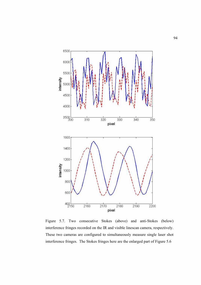
94
Figure 5.7. Two consecutive Stokes (above) and anti-Stokes (below)
interference fringes recorded on the IR and visible linescan camera, respectively.
These two cameras are configured to simultaneously measure single laser shot
interference fringes. The Stokes fringes here are the enlarged part of Figure 5.6

95
It is then easy to quantify the fringe movement by the phase difference between two
successive camera-recorded fringes. Remember the camera is operating at a much lower
frame rate than the laser pulse repetition rate, and in this sense, the consecutive fringes
are not the same as consecutive laser shots. Typically, the time delay between two
consecutive fringes is about 30 ms. Mathematically, the phase extracted from one
combined fringe containing both first-order Stokes and anti-Stokes that are
simultaneously taken by two cameras can be written as:
Figure 5.8. Example of extracting phase from Stokes interference
fringe (blue dotted) by performing sinusoidal fit (red solid)

96
(1) ( ) ( ) (1) (1)1 1 1 0 1
A B
(1) ( ) ( ) (1) (1)1 1 1 0 1
A B (5-6)
where the superscript A and B on the right side of the equation counts the fiber number,
and the number superscript of the left hand side is the fringe number. The symbol
denotes the phase difference between the two fibers. For two consecutive camera-
recorded fringes, the phase differences, or the movement of the Stokes and anti-Stokes
fringes, are:
(2) (1)
1 1 1 , (2) (1)
1 1 1 . (5-7)
According to our theoretical predictions, the phases of first-order Stokes and anti-
Stokes are anti-correlated in one pump pulse, that is, ( ) ( )1 1 constantn n . In this
sense, the summation of the two-phase differences between consecutive camera-recorded
fringes from two fibers should be zero:
(2) (1) (2) (1) (2) (2) (1) (1)
1 1 1 1 1 1 1 1 1 1( ) ( ) 0 (5-8)
In the experiment, the probability distribution of 1 1 is obtained by analyzing
over 300 experimentally recorded data (simultaneously recorded Stokes and anti-Stokes
fringes), and is plotted in Figure 5.9. Its narrow peak around zero clearly shows the
predicted phase anti-correlation between first-order Stokes and anti-Stokes. Using this

97
probability distribution, we calculate the quantity 1 1( )ie , which quantifies the
degree of phase anti-correlation:
1 1( ) 0.8ie
(5-9)
Our theoretical prediction for this quantity based on quantum Raman theory (see
Chapter III, Section 1) is nearly one. This discrepancy between experiment results and
theoretical prediction indicates the Raman comb process is more complicated than the
first-order rigorous theory accounts for. In this sense, more sidebands need to be
considered in the future development of the theory.
Figure 5.9. Histogram plot showing the probability distribution of
the anti-correlation phase ( 1 1 ).

98
As we mentioned previously, this phase anti-correlation between Stokes and anti-
Stokes fields is spontaneously generated. For the individual comb line, its phase is totally
random. In Figure 5.10 I plot the histograms of the Stokes and anti-Stokes phases from
the experimental data that is used to plot Figure 5.9. It’s clear that both phases are
random from one shot to another.
Figure 5.10. Random phases of Stokes (a) and anti-Stokes fields (b)
(b)
(a)

99
Synchronize two cameras
In the previous section, we showed how we verified the phase anti-correlation
between first-order Stokes and anti-Stokes fields. The essential idea is to observe the
interference fringes of these two fields that are generated from two independent
hydrogen-filled HCPCFs simultaneously on two cameras. Here, this simultaneous
measurement ensures that the two cameras capture the Raman fields generated by the
same single-pump pulse. Otherwise, the measurement of the probability distribution of
1 1 would not show any narrow peak, unless there is any phase correlation
between Stokes or anti-Stokes fields that are generated by two pump pulses that are at
least a few milliseconds apart. However, the molecular coherence usually fast dissipates
in nanosecond scale, and therefore, the second pump pulse will not see any footprint that
the first pump left in the molecules, and the fields it generated should have random
phases compared to the phases of fields generated by the first pump.
In this section, I will show that in the experiment we ensured the two cameras were
operating simultaneously (or synchronized), and the experiment result of measuring the
probability distribution of 1 1 if the two pumps are not synchronized.
In principle, although the two cameras we use are manufactured by different
companies, both cameras are operating similarly. Their operation principle can be
summarized as following: First, they will receive an ‘open connection’ command from
100
the computer. Under this command, the camera will first clear the memory of old data in
its physical memory part, and then wait for a ‘start measurement’ command. Once it
receives one, the camera will then wait for a trigger signal, which usually is a TTL from
low to high pulse. After it’s triggered, the camera will start ‘integration’ for a period of
time set in its operating mode parameters, which means all the photons registered during
this specified time period will be converted into electron currents.
However, since the IR and visible cameras are made from different companies, they
are slightly different in their response times. This response time is defined as the time
delay between receiving the computer command for ‘start’ and actually starting to
integrate. If the response times of both cameras are shorter than the pulse repetition rate,
which is 200 ms, then both cameras will be active for the same pump pulse.
Unfortunately, our cameras are not fast enough in this time scale. Also, the response time
difference is longer than 200 ms, which means the two cameras will naturally operate
asynchronously.
To synchronize two cameras, the trick is to use an external trigger signal in a slow
repetition rate. Normally, this external trigger is generated from the photo-detector that
detects the light signal picked off from the pump pulse train, which is at 5 KHz. However,
we can bring it down by the frequency divider, and this will slow the ‘effective’ pulse
repetition rate that the two cameras are operating at. Once the response time difference
between two cameras is shorter than this effective rate, the two cameras will be activated
for same pump pulse; in other words, they’ll be synchronized. The negative side effect is
the slow detection rate (or frame rate). Usually we operate the two cameras synchronized

101
at about 30 frames per second, lower than the typical 100 frames per second that we used
in the previous experiment that uses only one individual camera to measure the Stokes
energy statistics.
We test the synchronization of two cameras in the following way: A chopper wheel is
placed in the alignment before the pump light is split by first beam-splitter (BS-A in
Figure 5.5). This chopper wheel is operating at 1.7 KHz to modulate the pump’s intensity.
The two cameras are both configured in slow trigger mode and ‘simultaneously’ detect
the pump signal transmitted from the HCPCF fiber. In Figure 5.11 we show the signal
recorded from two cameras versus the frame (or detection) number. The vertical axis is
the peak amplitude of the pump signal recorded on each camera in one ‘simultaneous’
detection numbered by the horizontal axis. We can see that these peak amplitudes from
the two cameras are oscillating together due to the amplitude modulation from the
chopper wheel, which directly shows the two cameras are correctly synchronized in our
experiment.

102
I also performed the measurement of the probability distribution of 1 1 with
the same procedures described in the previous section, but with ‘asynchronous’ cameras.
The result is plotted in Figure 5.12. We see a random phase distribution, which exactly
shows no phase correlation between the Stokes field generated by the first pump pulse
and the anti-Stokes field generated by another pump pulse following the first one by a
few milliseconds. Or, in other words, no molecular seeding is present in our experiment
with a 5 kHz pump repetition rate.
Figure 5.11. Simultaneous measurement of pump signals on two
cameras. The pump’s amplitude is modulated by a chopper wheel
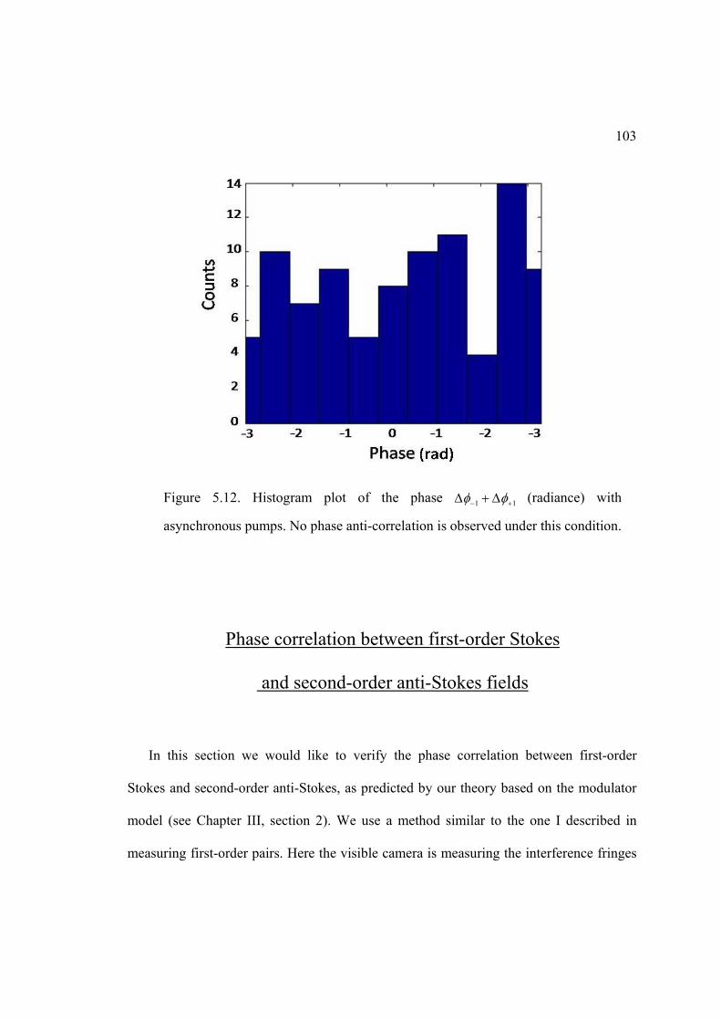
103
Phase correlation between first-order Stokes
and second-order anti-Stokes fields
In this section we would like to verify the phase correlation between first-order
Stokes and second-order anti-Stokes, as predicted by our theory based on the modulator
model (see Chapter III, section 2). We use a method similar to the one I described in
measuring first-order pairs. Here the visible camera is measuring the interference fringes
Figure 5.12. Histogram plot of the phase 1 1 (radiance) with
asynchronous pumps. No phase anti-correlation is observed under this condition.
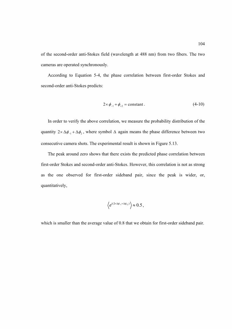
104
of the second-order anti-Stokes field (wavelength at 488 nm) from two fibers. The two
cameras are operated synchronously.
According to Equation 5-4, the phase correlation between first-order Stokes and
second-order anti-Stokes predicts:
1 22 constant . (4-10)
In order to verify the above correlation, we measure the probability distribution of the
quantity 1 22 , where symbol again means the phase difference between two
consecutive camera shots. The experimental result is shown in Figure 5.13.
The peak around zero shows that there exists the predicted phase correlation between
first-order Stokes and second-order anti-Stokes. However, this correlation is not as strong
as the one observed for first-order sideband pair, since the peak is wider, or,
quantitatively,
1 2(2 ) 0.5ie ,
which is smaller than the average value of 0.8 that we obtain for first-order sideband pair.

105
The reasons why the correlation is degraded for higher-order modes is not well
understood. We speculate that dispersion between second-order Stokes and first-order
Stokes may be an important factor.
Two-color experiment
The key idea in our derivation of the phase correlation involving high-order
sidebands in Chapter III is the so-called phase modulation. This idea assumes that the
Figure 5.13. Histogram showing the probability
distribution of quantity 1 22 .
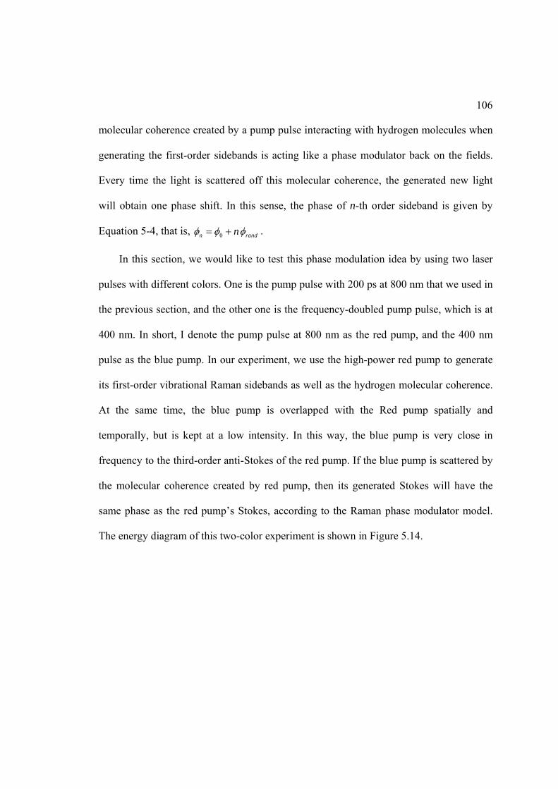
106
molecular coherence created by a pump pulse interacting with hydrogen molecules when
generating the first-order sidebands is acting like a phase modulator back on the fields.
Every time the light is scattered off this molecular coherence, the generated new light
will obtain one phase shift. In this sense, the phase of n-th order sideband is given by
Equation 5-4, that is, 0n randn .
In this section, we would like to test this phase modulation idea by using two laser
pulses with different colors. One is the pump pulse with 200 ps at 800 nm that we used in
the previous section, and the other one is the frequency-doubled pump pulse, which is at
400 nm. In short, I denote the pump pulse at 800 nm as the red pump, and the 400 nm
pulse as the blue pump. In our experiment, we use the high-power red pump to generate
its first-order vibrational Raman sidebands as well as the hydrogen molecular coherence.
At the same time, the blue pump is overlapped with the Red pump spatially and
temporally, but is kept at a low intensity. In this way, the blue pump is very close in
frequency to the third-order anti-Stokes of the red pump. If the blue pump is scattered by
the molecular coherence created by red pump, then its generated Stokes will have the
same phase as the red pump’s Stokes, according to the Raman phase modulator model.
The energy diagram of this two-color experiment is shown in Figure 5.14.

107
The blue pump is generated by a second harmonic generation of the red pump on a
BBO crystal. We choose to use a BBO crystal because it is a uniaxial crystal with a high
damage threshold. We carefully designed this BBO crystal optimized for 200 ps pulses.
The cutting of the BBO crystal is set at an angle c (the angle between the crystal’s
optical axis and the normal to the crystal surface) so that we can use the type I second
harmonic generation, where two red photons at 800 nm with polarization at the crystal’s
ordinary refractive index axis are annihilated and one blue photon at 400 nm with
polarization at the crystal’s extraordinary refractive index axis is produced. The critical
angle for the phase mismatching condition at this situation is about 24 degrees. This
angle can be achieved by putting the crystal on a rotational stage.
Figure 5.14. Energy diagram of the two-color experiment
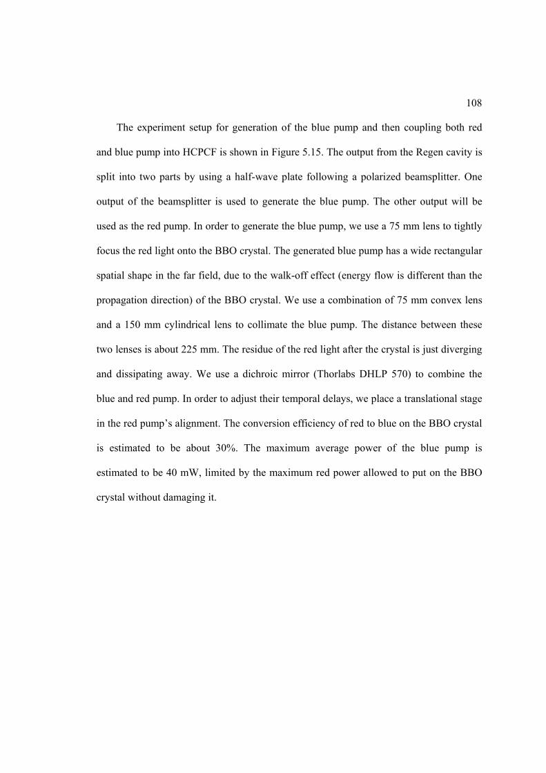
108
The experiment setup for generation of the blue pump and then coupling both red
and blue pump into HCPCF is shown in Figure 5.15. The output from the Regen cavity is
split into two parts by using a half-wave plate following a polarized beamsplitter. One
output of the beamsplitter is used to generate the blue pump. The other output will be
used as the red pump. In order to generate the blue pump, we use a 75 mm lens to tightly
focus the red light onto the BBO crystal. The generated blue pump has a wide rectangular
spatial shape in the far field, due to the walk-off effect (energy flow is different than the
propagation direction) of the BBO crystal. We use a combination of 75 mm convex lens
and a 150 mm cylindrical lens to collimate the blue pump. The distance between these
two lenses is about 225 mm. The residue of the red light after the crystal is just diverging
and dissipating away. We use a dichroic mirror (Thorlabs DHLP 570) to combine the
blue and red pump. In order to adjust their temporal delays, we place a translational stage
in the red pump’s alignment. The conversion efficiency of red to blue on the BBO crystal
is estimated to be about 30%. The maximum average power of the blue pump is
estimated to be 40 mW, limited by the maximum red power allowed to put on the BBO
crystal without damaging it.
109
The combined blue and red pumps are then coupled into a two-fiber setup, similar to
the one shown in Figure 5.11. Both red and blue pumps are coupled into each fiber. The
difficulty, however, is how to diminish the chromatic aberration in the focusing lenses,
since the two pumps are widely separate in wavelength. Thanks to the large numerical
aperture of the HCPCF (NA>0.03), we don’t need to use a tightly focused coupling lens,
such as a microscopic objective lens. In Gaussian optics theory, if the laser beams are
focused by a lens with a long focal length, then they will have longer Raleigh ranges at
their focal spots. If the chromatic aberration focal shift of the blue and red pumps induced
Figure 5.15. Experimental setup for two-color experiment

110
by the coupling lens is smaller than their Raleigh range, then it’s possible to couple both
beams into HCPCF with high efficiency. In the experiment, we use a 50 mm achromatic
doublet lens with broadband visible to near-infrared coating. Note that this lens is
different than the one (focal length is 35mm) optimized for a single-pump situation. In
this way we slightly compromise the coupling efficiency of the red pump to significantly
increase the blue coupling efficiency. We estimate that the coupling efficiency of the red
and blue pump is about 15% and 20%, respectively.
In Figure 5.16, we also show the Raman spectrum generated with both pumps
coupled into one HCPCF. The blue pump is controlled at low intensity, so that it does not
generate any sidebands by itself. However, with the red pump interacting strongly with
hydrogen molecules, the blue pump is scattered by the molecules that are coherently
excited by the red pump and its first-order Stokes is present in the spectrum. It should be
noted that, in Figure 5.16, the red pump looks dimmer than the blue pump although the
red pump is 20 times more intense than the blue pump. This is because the blue color is
more sensitive to the digital camera. In Figure 5.17, we show the picture of “colorful”
fibers when the two-color experiment is taking place.
Figure 5.16. Raman spectrum generated in two-color experiment
111
We also perform the simultaneous phase measurement of first-order Stokes of the
blue pump (at 485 nm) and first-order anti-Stokes of the red pump (at 602 nm). From
their single-shot interference fringes recorded on one visible linescan camera (Thorlabs),
which automatically ensures the simultaneous measurement, we can obtain the
probability distribution of the quantity blue redstokes anti stokes . The typical individual
interference fringes (single shots) are shown in Figure 5.18.
Figure 5.17. Picture of fiber when two-color experiment is taking place
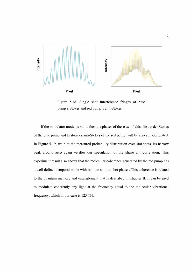
112
If the modulator model is valid, then the phases of these two fields, first-order Stokes
of the blue pump and first-order anti-Stokes of the red pump, will be also anti-correlated.
In Figure 5.19, we plot the measured probability distribution over 300 shots. Its narrow
peak around zero again verifies our speculation of the phase anti-correlation. This
experiment result also shows that the molecular coherence generated by the red pump has
a well-defined temporal mode with random shot-to-shot phases. This coherence is related
to the quantum memory and entanglement that is described in Chapter II. It can be used
to modulate coherently any light at the frequency equal to the molecular vibrational
frequency, which in our case is 125 THz.
Figure 5.18. Single shot Interference fringes of blue
pump’s Stokes and red pump’s anti-Stokes

113
Phase locking the Raman comb
Our experiment results using single pump to generate the optical Raman frequency
comb clearly verify two predictions of our theoretical work: the random phases from shot
to shot and the phase correlation among comb lines in one shot. In order to overcome this
phase randomness, people add an auxiliary laser beam with the pump beam to coherently
drive the molecular vibration, and thus the generated comb has a locked phase [65]. Often,
this auxiliary laser beam is spectrally overlapped with the first-order Stokes line. One
Figure 5.19. Experiment result of the probability
distribution (histogram) of the quantity blue redstokes anti stokes .
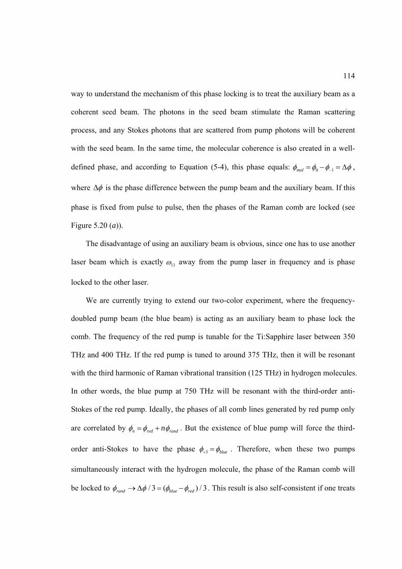
114
way to understand the mechanism of this phase locking is to treat the auxiliary beam as a
coherent seed beam. The photons in the seed beam stimulate the Raman scattering
process, and any Stokes photons that are scattered from pump photons will be coherent
with the seed beam. In the same time, the molecular coherence is also created in a well-
defined phase, and according to Equation (5-4), this phase equals: 0 1mol ,
where is the phase difference between the pump beam and the auxiliary beam. If this
phase is fixed from pulse to pulse, then the phases of the Raman comb are locked (see
Figure 5.20 (a)).
The disadvantage of using an auxiliary beam is obvious, since one has to use another
laser beam which is exactly 13 away from the pump laser in frequency and is phase
locked to the other laser.
We are currently trying to extend our two-color experiment, where the frequency-
doubled pump beam (the blue beam) is acting as an auxiliary beam to phase lock the
comb. The frequency of the red pump is tunable for the Ti:Sapphire laser between 350
THz and 400 THz. If the red pump is tuned to around 375 THz, then it will be resonant
with the third harmonic of Raman vibrational transition (125 THz) in hydrogen molecules.
In other words, the blue pump at 750 THz will be resonant with the third-order anti-
Stokes of the red pump. Ideally, the phases of all comb lines generated by red pump only
are correlated by n red randn . But the existence of blue pump will force the third-
order anti-Stokes to have the phase 3 blue . Therefore, when these two pumps
simultaneously interact with the hydrogen molecule, the phase of the Raman comb will
be locked to / 3 ( ) / 3rand blue red . This result is also self-consistent if one treats
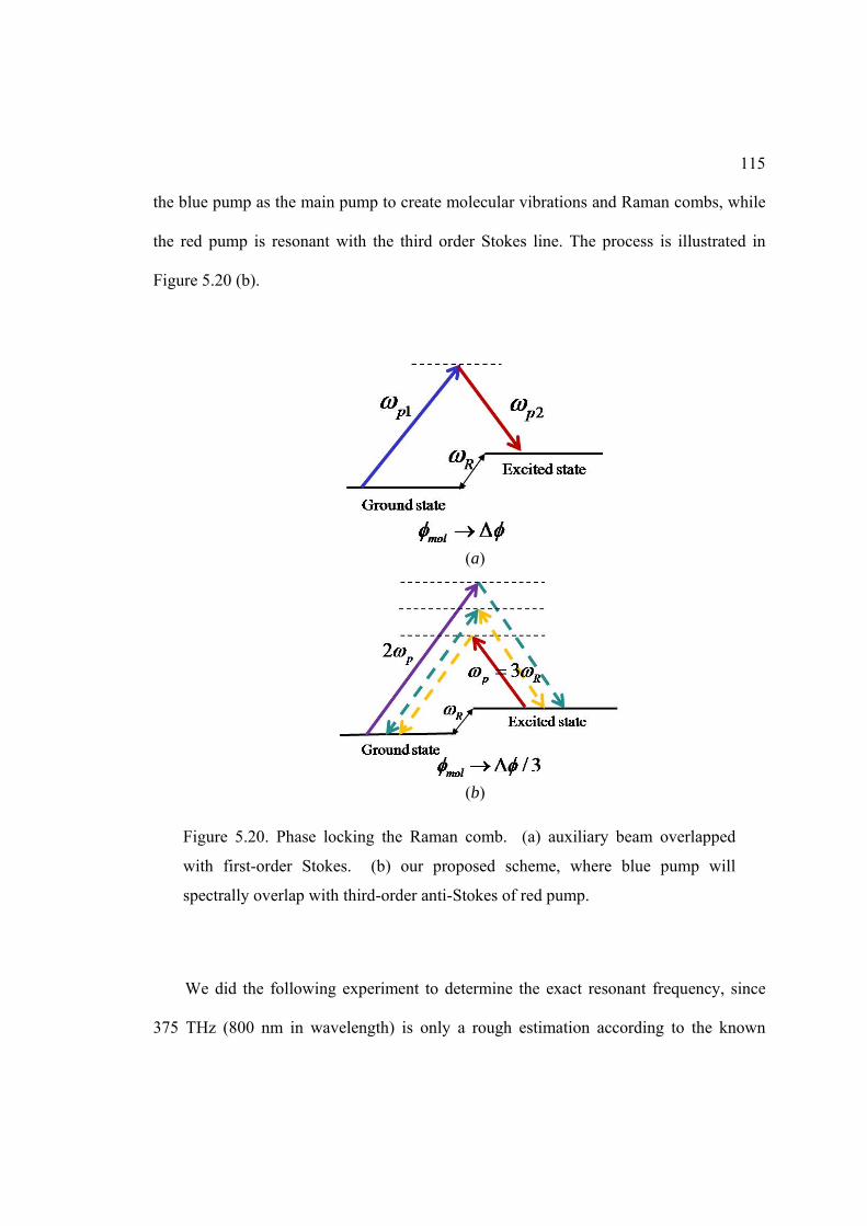
115
the blue pump as the main pump to create molecular vibrations and Raman combs, while
the red pump is resonant with the third order Stokes line. The process is illustrated in
Figure 5.20 (b).
(a)
(b)
We did the following experiment to determine the exact resonant frequency, since
375 THz (800 nm in wavelength) is only a rough estimation according to the known
Figure 5.20. Phase locking the Raman comb. (a) auxiliary beam overlapped
with first-order Stokes. (b) our proposed scheme, where blue pump will
spectrally overlap with third-order anti-Stokes of red pump.

116
hydrogen Raman transition frequency. We use a strong red beam (no blue beam) to
generate the Raman comb in one fiber filled with 100 PSI hydrogen in its loading cell,
and filter out the third-order anti-Stokes line at around 400 nm. In the other fiber, no
hydrogen is filled and only a blue pump, which is directly generated from the BBO
crystal, is transmitted through the fiber. We spatially overlap this blue pump and the
third-order anti-Stokes generated by the red pump in the other fiber, and record the
interference fringes on one visible line-scan camera while tuning the red pump laser
around 800 nm.
Since the amplitude and phase of the third-order anti-Stokes is fluctuating, the
visibility of the recorded interference fringes at one certain laser wavelength is also
changing. We analyze each fringe by using the sinusoidal fit that is described in the
previous section (Figure 5.8), and extract the amplitude of the fit. For one wavelength
point, we obtain the average of the interference amplitudes of 100 fringes, and plot this
average amplitude as a function of the wavelength. The result is shown in Figure 5.21.
We can see that the resonant wavelength is clearly shown at 802.2150 nm. This, in
turn, can be used to deduce the Raman vibrational frequency shift of hydrogen molecule.
We found it to be 4155.16 cm-1, very close to the one used as a standard value (4155.23
cm-1) [37]. After we found this resonant wavelength, we coupled both the blue and red
pumps into two fibers. Since the proposed phase locking uses a third-order effect, it
requires the blue pump’s power as high as the red pump’s. The experiment setup (Figure
5.15) in the “two-color experiment” section is no longer suitable, because the blue
pump’s power is limited by how much Regen output is split onto BBO crystal. We are

117
currently modifying the setup, basically to allow us to use full Regen output onto the
BBO crystal to generate the blue pump. In this way, we believe the blue pump will be
strong enough so that we can observe the phase-locked comb.
Figure 5.21. Average amplitude of interference fringes as
a function of wavelength tuning
118
CHAPTER VI
CONCLUSIONS
With the help of hollow-core photonic crystal fiber, Raman optical frequency comb
generation now looks achievable with relatively low-power table-top setups. In our
experiment, we have demonstrated that, with one stage of amplification, a Ti:Sapphire
laser is capable to generate more than 20 rotational or 4 vibrational comb lines at the
energy level of 10 micro-joules per pulse. The total frequency span of the optical Raman
comb is multiple octaves, where the highest frequency is a factor of 2 or larger than the
lowest frequency.
In comparison, conventional Raman comb experiments carried out using meter-long
high-pressure hydrogen tubes requires Q-switched high-power lasers with fixed output
wavelength. he frequency tuning capability of Ti:Sapphire laser will then have another
comparative advantage, that is, it will allow the generated Raman comb to cover all
frequencies from blue to infrared region. To reach the deep blue region (< 350 nm), one
can first frequency double the Ti:Sapphire laser output, as described in our two-color
experiment, and then generate the Raman frequency comb from the frequency-doubled
light.
119
An individual Raman comb line can be used as a reliable laser source, if the Raman
comb is phase stabilized by coherent seeding. The portability and easy construction of the
gas-filled HCPCF will make the Raman comb a very useful light source for those
applications requiring multiple lasers.
Our goal of using the Raman optical frequency comb is to synthesize atto-second
pulses, which are short enough for illuminating an electron’s motion. Since we only use
a single pump pulse, all Stokes and anti-Stokes lines are generated from quantum vacuum
fluctuations. By simply making an analogy between first-order Raman generation and
the four-wave mixing (FWM) process, we speculate that there are phase correlations in
the generated first-order Stokes and anti-Stokes fields. However, in Raman scattering, the
molecular vibration needs to take into consideration, which is neglected in standard
FWM theory. Our speculation is confirmed by first using quantum theory to model the
Raman process, and then calculating the value of an anti-correlation coefficient under the
initial conditions directly reflecting the quantum initiation of the comb lines. This anti-
correlation coefficient not only predicts that the energy of first-order Stokes and anti-
Stokes are fluctuating in the same manner, but their phases sum to a constant from shot to
shot. This quantum initiated phase correlation has never been observed in experiment
before, nor has anyone attempted to illustrate it. Our collaborators in University of Bath
first observed this phase correlation [66], and later we confirmed it by using 200 pico-
second Raman pump pulses generating H2 vibrational comb lines [67].
In our experiments, we set up an interferometer that contains two quantum initiated
Raman optical frequency combs. These two Raman combs are regarded as identical,
120
since they are pumped by pump pulses with identical properties, the same HCPCF type
and length are used, and the same hydrogen gas pressure is used. The outputs of the
interferometer are interference fringes of pairs of comb lines having the same order,
which were filtered from the two Raman combs. The high visibility of these interference
fringes shows that the Raman combs are generated in near transform limited pulses. By
recording the single-shot interference fringes of first-order Stokes and anti-Stokes
simultaneously from the two outputs of the interferometer, and observing their
movements from one pump shot to another, we illustrate the expected phase correlation
between first-order sidebands. Using the same method, we can also show that phase
correlation also exists for higher order sidebands. This phase correlation can be explained
by a self-consistent Raman modulator model, where hydrogen molecules are excited by a
pump pulse and act as a phase modulator to all comb lines.
The Raman modulator model is a simple and useful guideline for predicting the
mechanism of Raman comb generation. We tested the idea of Raman modulator model
by setting up a two color experiment. This experiment illustrates that the molecular
vibration created in the quantum initiated Raman scattering process has a well defined
(that is, constant throughout the pulse) phase, but that the value of this phase is random.
This random phase determines the phase of generated Stokes and anti-Stokes fields. If
any other light field is scattered by the molecular coherence, its scattered field will obtain
this random phase shift, the same as if the light is being phase modulated by the
molecular coherence.

121
This discovery of phase correlation in Raman comb lines leads us to develop a new
method for phase locking the comb. According to our understanding from the Raman
modulator model, phase locking the comb is equivalent to stabilizing the phase of
molecular coherence. If the Raman pump is tuned to an integer multiple of the natural
frequency ( 13 ) of molecular vibration (or rotation), then its second harmonic and itself,
whose frequency difference will also be multiple integer times 13 , will force the
molecules to vibrate in a well defined phase related to their phase difference. People have
demonstrated this phase locking effect in hydrogen gas when the pump frequency equals
13 , the hydrogen vibrational frequency, and we are currently carrying out an experiment
where the pump frequency will be three times 13 . This frequency happens to fall into
the Ti:Sapphire region, around 800 nm in wavelength. If our experiment is successful, the
phasing-locking scheme will be greatly simplified because when different Raman active
medium is used, it will no longer be limited by the availability of lasers operating at
Raman transition frequency.

122
APPENDIX A
DETAILED EXPRESSION FOR CALCULATING ANTI-
CORRELATION COEFFICIENT
Here we give the detailed expressions for the correlation coefficient C that is defined
in equation (3-5), and for the intensity of the first-order Stokes and anti-Stokes fields, by
using the solution of equation (3-2) and the initial conditions of equation (3-4). The
Stokes intensity is:
( ) ( )1 1
2 22
2 2 2 22, 1 2, 1,
0 13 0 0 120 0
( , ) ( , ) ( , )
2( ) ( ; ,0) ( ) ( ) ( ; , )
s
La s a
I L E L E L
E dz G z E d E G LAN Ac
(A1)
The anti-Stokes intensity is:
22
2 21 1, 2,( ) ( )1 1 0 0 210
2( , ) ( , ) ( , ) ( ) ( ) ( ; , )
s a
aI L E L E L E d E G LAc
(A2)
The product of Equation (A1) and (A2) gives the denominator of correlation coefficient
C, and its numerator is:
22 *2 2 21 1, 2, 2,( ) ( ) *
1 1 0 0 11 120
2( , ) ( , ) ( ) ( ) ( ; , ) ( ; , )
s s aE L E L E d E G L G L
Ac
(A3)
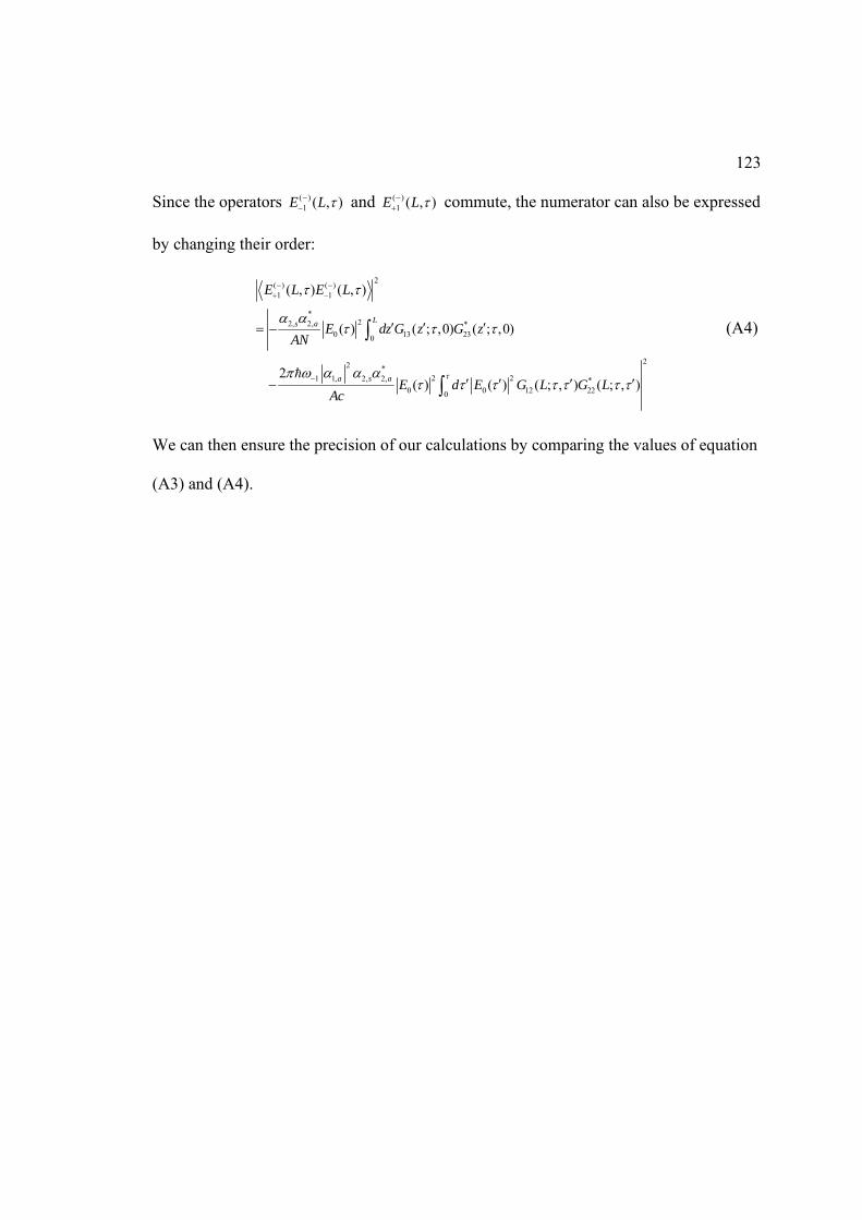
123
Since the operators ( )1 ( , )E L and ( )
1 ( , )E L commute, the numerator can also be expressed
by changing their order:
2( ) ( )1 1
*22, 2, *
0 13 230
22 *2 21 1, 2, 2, *
0 0 12 220
( , ) ( , )
( ) ( ; ,0) ( ; ,0)
2 ( ) ( ) ( ; , ) ( ; , )
Ls a
a s a
E L E L
E dz G z G zAN
E d E G L G LAc
(A4)
We can then ensure the precision of our calculations by comparing the values of equation
(A3) and (A4).

124
APPENDIX B
PULSE MEASURING DEVICE
This is an independent project that I have worked in parallel with my main research
topic in Raman optical frequency comb generation. Our goal of this project is to
characterize the amplitude and envelope phase of mode-lock laser pulses whose duration
is approximately 100 pico-seconds. These pulses cannot be measured by conventional
pulse characterization devices, such as FROG [68], because their spectrum spreading is
too small to be measured accurately.
First of all, we need to define what we mean by the envelope phase of an optical pulse.
This phase is the temporal phase of the slowly-changing envelope of the electric field.
Mathematically, the optical pulse can be written as:
0( )( ) ( ) i ti tE t E t e e .
where 0 is the optical frequency at about 400 THz, ( )t is the phase that we want to
measure, and ( )E t is the amplitude.
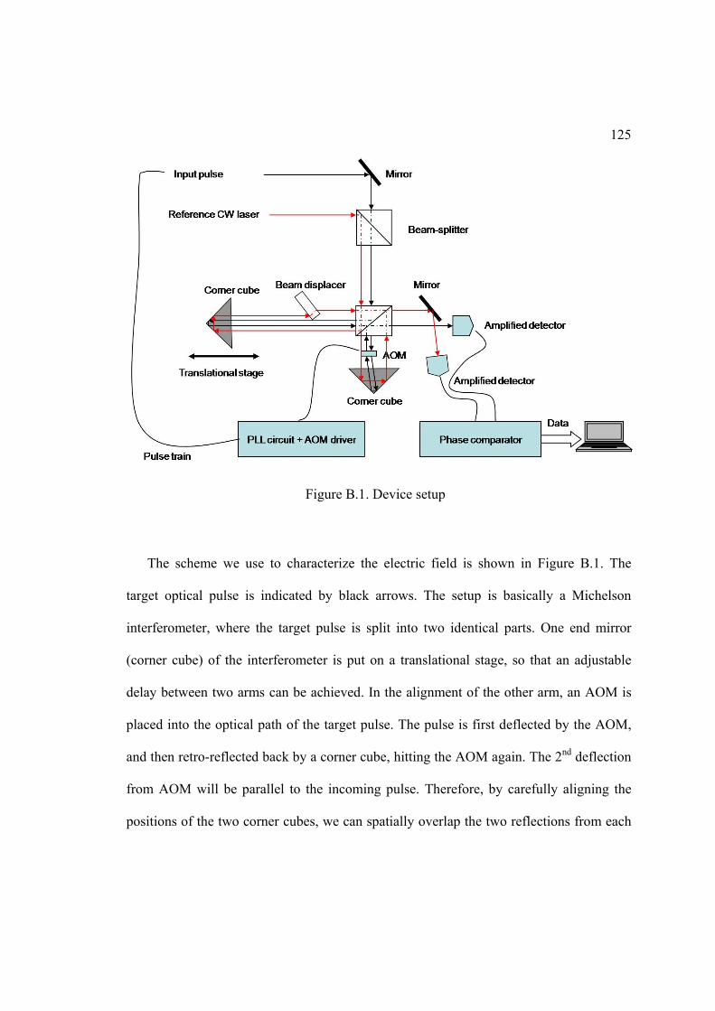
125
The scheme we use to characterize the electric field is shown in Figure B.1. The
target optical pulse is indicated by black arrows. The setup is basically a Michelson
interferometer, where the target pulse is split into two identical parts. One end mirror
(corner cube) of the interferometer is put on a translational stage, so that an adjustable
delay between two arms can be achieved. In the alignment of the other arm, an AOM is
placed into the optical path of the target pulse. The pulse is first deflected by the AOM,
and then retro-reflected back by a corner cube, hitting the AOM again. The 2nd deflection
from AOM will be parallel to the incoming pulse. Therefore, by carefully aligning the
positions of the two corner cubes, we can spatially overlap the two reflections from each
Figure B.1. Device setup

126
corner cube on the beamsplitter. The output of the interferometer is then detected by an
amplified detector (Thorlabs PDA100A).
Double passing through the AOM is actually spectrally shearing [69] the optical pulse,
which means the resultant pulse is identical to the original pulse except that it is
frequency shifted by certain amount ( ). In another hand, the Michelson interferometer
output, usually called auto-correlation signal, is well known as the Fourier transform of
the power spectrum of the pulse. We then can show that the signal on amplified detector
is:
0( )( ) ( ) ( ) . .ii if d E E e e e c c , (B-1)
where /L c is the delay between the two arms of the interferometer. It contains the
information of interest, i.e., the slowly-varying phase term (in frequency domain):
( ) ( ) ( ) . (B-2)
It is our purpose of this experiment to retrieve this phase difference ( ) from the
detected signals (equation B-1) on the amplified detector, which can be measured as a
function of the delay . A well established concatenation method then can be used to
retrieve the spectral phase ( ) [69].
In theory, if we can obtain the quantity shown in the bracket of equation B-1, that is,
( ) ( )( ) ( ) ( ) ( )i i iI d E E e e I e , (B-3)
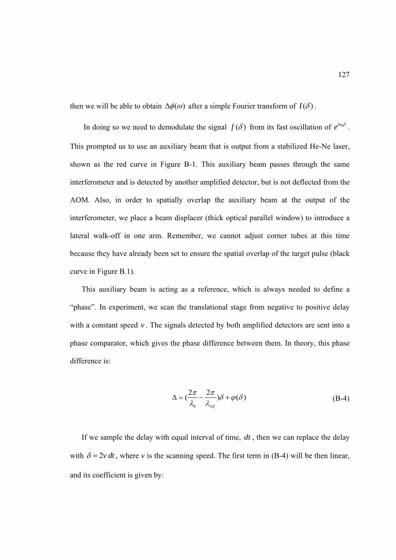
127
then we will be able to obtain ( ) after a simple Fourier transform of ( )I .
In doing so we need to demodulate the signal ( )f from its fast oscillation of 0ie .
This prompted us to use an auxiliary beam that is output from a stabilized He-Ne laser,
shown as the red curve in Figure B-1. This auxiliary beam passes through the same
interferometer and is detected by another amplified detector, but is not deflected from the
AOM. Also, in order to spatially overlap the auxiliary beam at the output of the
interferometer, we place a beam displacer (thick optical parallel window) to introduce a
lateral walk-off in one arm. Remember, we cannot adjust corner tubes at this time
because they have already been set to ensure the spatial overlap of the target pulse (black
curve in Figure B.1).
This auxiliary beam is acting as a reference, which is always needed to define a
“phase”. In experiment, we scan the translational stage from negative to positive delay
with a constant speed v . The signals detected by both amplified detectors are sent into a
phase comparator, which gives the phase difference between them. In theory, this phase
difference is:
0
2 2( ) ( )
ref
(B-4)
If we sample the delay with equal interval of time, dt , then we can replace the delay
with 2v dt , where v is the scanning speed. The first term in (B-4) will be then linear,
and its coefficient is given by:

128
0
1 14 ( )
ref
v
.
Therefore, after we obtain the experimental raw data from phase comparator, we first
do a linear fit, and the slope of the fit can be used to deduce the central wavelength 0 of
the target pulse. The residue value after subtracting the linear fit then gives the ( ) , the
phase term of ( )I . Amplitude of ( )I can be directly obtained from the amplitude of
interference signal from the amplified detector.
In Figure B.2, we plot the measurement result of Spectra-Physics Tsunami laser,
whose output (about 200 ps) is shown in Figure 4.6. The AOM is driven by a phase lock
loop circuit that is designed to lock the frequency at the Tsunami laser’s repetition rate,
about 80 MHz. By double passing through the AOM, the frequency shift of the shearing
laser is about 160 MHz. The estimated spectra width of the optical pulse is 2.2 GHz. The
ration between frequency shift and spectra width is about 7%, within the recommended
value of typical SPIDER technique [63].
The Fourier transform of auto-correlation data in Figure B.2(a) gives the power
spectrum of the optical pulse and the spectral phase. They are shown in Figure B.2(b) and
Figure B.2(c).
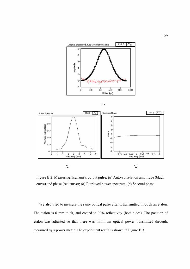
129
We also tried to measure the same optical pulse after it transmitted through an etalon.
The etalon is 6 mm thick, and coated to 90% reflectivity (both sides). The position of
etalon was adjusted so that there was minimum optical power transmitted through,
measured by a power meter. The experiment result is shown in Figure B.3.
Figure B.2. Measuring Tsunami’s output pulse: (a) Auto-correlation amplitude (black
curve) and phase (red curve); (b) Retrieved power spectrum; (c) Spectral phase.
(c) (b)
(a)
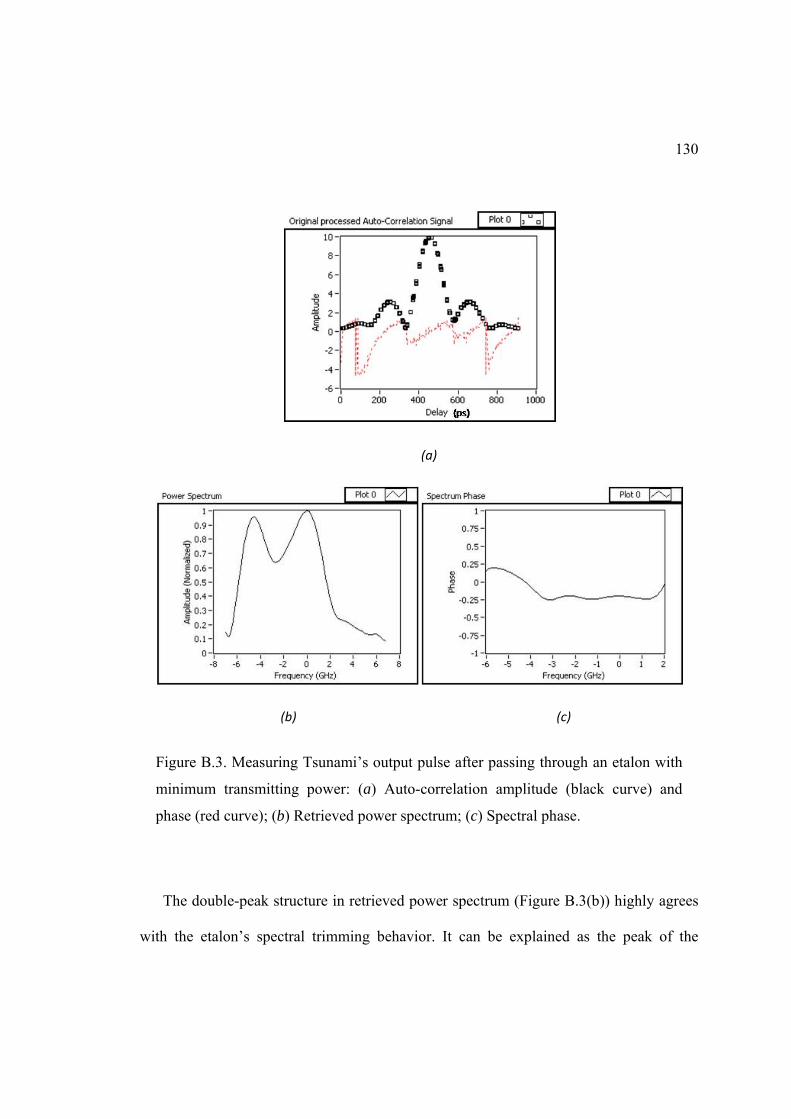
130
The double-peak structure in retrieved power spectrum (Figure B.3(b)) highly agrees
with the etalon’s spectral trimming behavior. It can be explained as the peak of the
Figure B.3. Measuring Tsunami’s output pulse after passing through an etalon with
minimum transmitting power: (a) Auto-correlation amplitude (black curve) and
phase (red curve); (b) Retrieved power spectrum; (c) Spectral phase.
(c) (b)
(a)
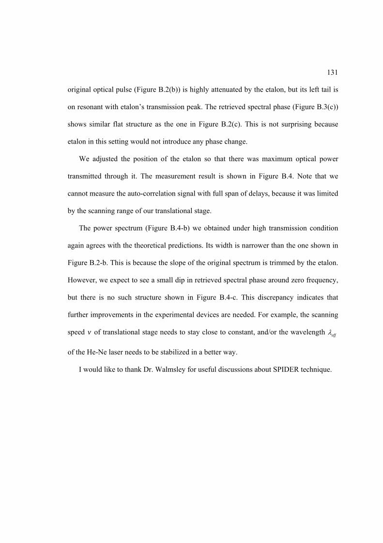
131
original optical pulse (Figure B.2(b)) is highly attenuated by the etalon, but its left tail is
on resonant with etalon’s transmission peak. The retrieved spectral phase (Figure B.3(c))
shows similar flat structure as the one in Figure B.2(c). This is not surprising because
etalon in this setting would not introduce any phase change.
We adjusted the position of the etalon so that there was maximum optical power
transmitted through it. The measurement result is shown in Figure B.4. Note that we
cannot measure the auto-correlation signal with full span of delays, because it was limited
by the scanning range of our translational stage.
The power spectrum (Figure B.4-b) we obtained under high transmission condition
again agrees with the theoretical predictions. Its width is narrower than the one shown in
Figure B.2-b. This is because the slope of the original spectrum is trimmed by the etalon.
However, we expect to see a small dip in retrieved spectral phase around zero frequency,
but there is no such structure shown in Figure B.4-c. This discrepancy indicates that
further improvements in the experimental devices are needed. For example, the scanning
speed v of translational stage needs to stay close to constant, and/or the wavelength eff
of the He-Ne laser needs to be stabilized in a better way.
I would like to thank Dr. Walmsley for useful discussions about SPIDER technique.

132
Figure B.4. Measuring Tsunami’s output pulse after passing through an etalon with
maximum transmitting power: (a) Auto-correlation amplitude (black curve) and
phase (red curve); (b) Retrieved power spectrum; (c) Spectral phase.
(c) (b)
(a)

133
BIBLIOGRAPHY
[1] M. Kourogi, K. Nakagawa and M. Ohtsu, “Wide-span optical frequency comb generation for accurate optical frequency difference measurement,” IEEE J. Quant. Electron. 29, 2693-2701 (1993) [2] H. A. Haus, “Short Pulse Generation,” in Compact Sources of Ultrashort Pulses, edit by I. N. Duling III, Cambridge University Press (1995) [3] D. J. Kuizenga and A. E. Siegman, “FM and AM Mode Locking of the Homogeneous Laser - Part I: Theory,” IEEE J. of Quantum Electron. 6, 694 (1970) [4] H. A. Haus, “A Theory of Forced Mode Locking,” IEEE J. Quant. Electron. 11, 323 (1975) [5] T. Udem, J. Reichert, R. Holzwarth, and T. W. Hansch, “Accurate measurement of large optical frequency differences with a mode-locked laser,” Opt. Lett. 24, 881 (1993) [6] T. Udem, J. Reichert, T. W. Hansch, and M. Kourogi, “Absolute optical frequency measurement of the cesium D2 line,” Phys. Rev. A 62, 031801 (2000) [7] Telle, H. R., G. Steinmeyer, A. E. Dunlop, J. Stenger, D. H. Sutter, and U. Keller, “Carrier-envelope offset phase control: A novel concept for absolute optical frequency control and ultrashort pulse generation,” Appl. Phys. B: Lasers Opt. 69, 327 (1999) [8] J. Ranka, R. Windeler and A. Stentz, “Visible continuum generation in air-silica microstructure optical fibers with anomalous dispersion at 800 nm,” Opt. Lett. 25, 25 (2000) [9] S. A. Diddams, D. Jones, Jun Ye, S. Cundiff, J. Hall, J. Ranka, R. Windeler, R. Holzwarth, Th. Udem and T. W. Hansch, “Direct link between microwave and optical frequencies with a 300 THz femtosecond laser comb,” Phys. Rev. Lett. 84, 5102 (2000) [10] Th. Udem, J. Reichert, R. Holzwarth and T. W. Hansch, “Absolute optical frequency measurement of the Cesium D1 line with a mode-locked laser,” Phys. Rev. Lett. 82, 3568 (1999) [11] S. A. Diddams, Th. Udem, J. C. Berquist, E. A. Curtis, R. E. Drullinger, L. Hollberg, W. M. Itano, W. D. Lee, C. W. Oates, K. R. Vogel and D. J. Wineland, “An optical clock based on a single trapped 199Hg+ ion,” Science 293, 825 (2001) [12] Nobelprize.org
134
[13] M. Drescher, M. Hentschel, R. Kienberger, G. Tempea, C. Sipelmann, G. A. Reider, P. B. Corkum and F. Krausz, “X-ray pulses approaching the attosecond frontier,” Science 291, 1923 (2001) [14] P. M. Paul, E. S. Toma, P. Breger, G. Mullot, F. Auge, Ph. Balcou, H. G. Muller and P. Agostini, “Observation of a train of attosecond pulses from high harmonic generation,” Science 292, 1689 (2001) [15] M Drescher et al, “Time-resolved atomic inner-shell spectroscopy,” Nature 419, 803 (2002) [16] A. Baltuska, Th. Udem, M. Ulberacker, M. Hentschel, E. Goulielmakis, Ch. Gohle, R. Holzwarth, V. S. Yakovlev, A. Scrinzi, T. W. Hansch and F. Krausz, “Attosecond control of electronic processes by intense light fields,” Nature 421, 611 (2003) [17] Hiroyuki Kawano, Yasuyuki Hirakawa and Totaro Imasaka, “Generation of High-Order Rotational Lines in Hydrogen by Four-Wave Raman Mixing in the Femtosecond Regime,” IEEE J. Quant. Electron. 34, 260 (1998) [18] M. Y. Shverdin, D. R. Walker, D. D. Yavuz, G. Y. Yin and S. E. Harris, “Generation of a Single-Cycle Optical Pulse,” Phys. Rev. Lett. 94, 033904 (2005) [19] Takayuki Suzuki, Masataka Hirai and Masayuki Katsuragawa, “Octave-Spanning Raman Comb with Carrier Envelope Offset Control,” Phys. Rev. Lett. 101, 243602 (2008) [20] M. G. Raymer, I. A. Walmsley, J. Mostowski and B. Sobolewska, “Quantum theory of spatial and temporal coherence properties of stimulated Raman scattering,” Phys. Rev. A 32, 332 (1985) [21] I. A. Walmsley and M. G. Raymer, “Observation of Macroscopic Quantum Fluctuations in Stimulated Raman Scattering,” Phys. Rev. Lett. 50, 962 (1983) [22] C. V. Raman and K. S. Krishnan, “A new type of secondary radiation,” Nature 121, 501 (1928) [23] G. Placzek, “The Rayleigh and Raman scattering,” in Handbuch der Radiologie, Band VI, edited by E. Marx (1934) [24] G. Eckhardt, R. W. Hellwarth, F. J. McClung, S. Schwarz, D. Weiner and E. Woodbury, “Stimulated Raman scattering from organic liquids,” Phys. Rev. Lett. 9 455, (1962) [25] D. J. Gardiner, “Practical Raman spectroscopy,” Springer-Verlag (1989)

135
[26] Y. R. Shen, “Quantum statistics of nonlinear optics,” Phys. Rev. 155, 921 (1967) [27] M. G. Raymer and I. A. Walmsley, “The quantum coherence properties of stimulated Raman scattering,” in Progress In Optics, edited by E. Wolf, Vol. XXVIII, 180 (1990) [28] Walmsey and M. G. Raymer, “Experimental study of the macroscopic quantum fluctuations of partially coherent stimulated Raman scattering,” Phys. Rev. A 33, 382 (1986) [29] L. M. Duan, M. D. Lukin, J. I. Cirac and P. Zoller, “Long-distance quantum commnunication with atomic ensembles and linear optics,” Nature 414, 413 (2001) [30] C. H. van der Wal, M. D. Eisaman, A. Andre, R. L. Walsworth, D. F. Phillips, A. S. Zibrov and M. D. Lukin, “Atomic memory for correlated photon states,” Science 301, 196 (2003) [31] C. W. Chou, H. de Riedmatten, D. Felinto, S. V. Polyakov, S. J. van Enk and H. J. Kimble, “Measurement-induced entanglement for excitation stored in remote atomic ensembles,” Nature 438, 828 (2005) [32] T. Chaneliere, D. N. Matsukevich, S. D. Jenkins, S. Y. Lan, R. Zhao, T. A. B. Kennedy and A. Kuzmich, “Quantum interference of electromagnetic fields from remote quantum memories,” Phys. Rev. Lett. 98, 113602 (2007) [33] S. Harris, “Electromagnetically Induced Transparency,” Physics Today 50, 36 (1997) [34] K. F. Reim, J. Nunn, V. O. Lorenz, B. J. Sussman, K. C. Lee, N. K. Langford, D. Jaksch and I. A. Walmsley, “Towards high-speed optical quantum memories,” Nature Phtonics 4, 218 (2010) [35] S. E Harris and A. V. Sokolov, “Subfemtosecond Pulse Generation by Molecular Modulation,” Phys. Rev. Lett. 81, 2894 (1998) [36] W. Chen, Zhi-Ming Hsieh, Shu Wei Huang, Hao-Yu Su, Chien-Jen Lai, Tsung-Ta Tang, Chuan-Hsien Lin, Chao-Kuei Lee, Ru-Pin Pan, Ci-Ling Pan and A. H. Kung, “Sub-Single-Cycle Optical Pulse Train with Constant Carrier Envelope Phase,” Phys. Rev. Lett. 100, 163906 (2008) [37] Zhi-Ming Hsieh, Chien-Jen Lai, Han-Sung Chan, Sih-Ying Wu, Chao-Kuei Lee, Wei-Jan Chen, Ci-Ling Pan, Fu-Goul Yee, and A. H. Kung, “Controlling the Carrier-Envelope Phase of Raman-Generated Periodic Waveforms,” Phys. Rev. Lett. 102, 213902 (2009)

136
[38] F. Couny, F. Benabid and P. S. Light, “Large-pitch Kagome-structured hollow-core photonic crystal fiber,” Optics Letters 31, 3574 (2006) [39] F. Couny, F. Benabid, P. J. Roberts, P. S. Light and M. G. Raymer, “Generation and Photonic Guidance of Multi-Octave Optical Frequency Combs,” Science 318, 1118 (2007) [40] M. G. Raymer and J. Mostowski, “Stimulated Raman scattering: Unified treatment of spontaneous initiation and spatial propagation,” Phys. Rev. A 24, 1980 (1981) [41] Hermann A. Haus, “Electromagnetic Noise and Quantum Optical Measurements,” Springer (2000), Chapter 12 [42] W. Wasilewski and M. G. Raymer, “Pairwise entanglement and readout of atomic-ensemble and optical wave-packet modes in travelling wave Raman interactions,” Phys. Rev. A 73 063816 (2006) [43] J. S. Bell, “Speakable and unspeakable in quantum mechanics,” Cambridge University Press (1987) [44] E. Shchukin and W. Vogel, “Universal measurement of quantum correlations of radiation,” Phys. Rev. Lett. 96, 200403 (2006) [45] W. Ji, C. Wu, S. J. van Enk and M. G. Raymer, “Mesoscopic entanglement of atomic ensembles through nonresonant stimulated Raman scattering”, Phys. Rev. A 75, 052305 (2007) [46] D. T. Smithey, M. Beck, M. G. Raymer and A. Faridani, “Measurement of the Wigner distribution and the density matrix of a light mode using optical homodyne tomography: Application to squeezed states and the vacuum,” Phys. Rev. Lett. 70, 1244 (1993) [47] M. G. Raymer, “Quantum state entanglement and readout of collective atomic-ensemble modes and optical wave-packets by stimulated Raman scattering,” J. Mod. Optics, 51, 1739–1759 (2004) [48] S. Ya. Kilin, “Transient Anti-Stokes Stimulated Raman Scattering: the Possibility of Observing Quantum Macroscopic Fluctuations,” Europhys. Lett. 5, pp 419-424 (1988) [49] M. D. Duncan, R. Mahon, J. Reintjes and L. L. Tankersley, “Parametric Raman gain suppression in D2 and H2,” Optics Letters 11, 803 (1986) [50] M. Belsley, D. T. Smithey, K. Wedding and M. G. Raymer, “Observation of extreme sensitivity to induced molecular coherence in stimulated Raman scattering,” Phys. Rev. A 48, 1514 (1993)
137
[51] S.J. Kuo, D.T. Smithey, and M.G. Raymer, “Spatial Interference of Macroscopic Light Fields from Independent Raman Sources, ” Phys. Rev. A (Rapid Commun.) 43, 4083 (1990) [52] I. A. Walmsley, M. G. Raymer, T. Sizer II, I. N. Duling III and J. D. Kafka, “Stabilization of Stokes pulse energies in the nonlinear regime of stimulated Raman scattering,” Opt. Commun. 53, 137 (1985) [53] C. Wu, M. G. Raymer, Y. Y. Wang and F. Benabid, “Quantum theory of phase correlations in optical frequency combs generated by stimulated Raman scattering,” to be published in Phys. Rev. A (2010) [54] Robert W. Boyd, “Nonlinear Optics,” Academic Press 2003, Chapter 10 [55] Supporting online material for reference 37 [56] J. Mostowski and M. G. Raymer, “Quantum Statistics in Nonlinear Optics,” Chapter 5 in “Contemporary Nonlinear Optics,” Edited by G. P. Agrawal and R. W. Boyd, Academic Press (1992) [57] J. C. Knight, T. A Birks, P. St. J. Russell and D. M. Atkin, “All-silica single-mode optical fiber with photonic crystal cladding,” Optics Letters 21, 1547 (1996) [58] R. F. Cregan, B. J. Mangan, J. C. Knight, T. A. Birks, P. St. J. Russell, P. J. Roberts and D. C. Allan, “Single-mode photonic band gap guidance of light in air,” Science 285, 1537 (1999) [59] J. H. Neumann and E. Wigner, “On the behavior of eigenvalues in adiabatic processes,” Phys. Z. 30, 465 (1929) [60] F. H. Stillinger, D. R. Herrick, “Bound state in the continuum,” Phys. Rev. A 11, 446 (1975) [61] Andrew Funk Ph. D. Dissertation, University of Oregon library (2004) [62] P. Lallemand, P. Simova and G. Bret, “Pressure-induced line shift and collisional narrowing in hydrogen gas determined by stimulated Raman emission,” Phys. Rev. Lett. 17, 1239 (1966) [63] F. Benabid, G. Antonopoulos, J. C. Knight and P. St. J. Russell, “Stokes Amplification Regimes in Quasi-cw Pumped Hydrogen-Filled Hollow-Core Photonic Crystal Fiber,” Phys. Rev. Lett. 95, 213903 (2005)
138
[64] Mandel and Wolf, “Optical coherence and quantum optics,” Cambridge University Press (1995) [65] Hiroyuki Otsuka, Tomohiro Uchimura, and Totaro Imasaka, “Phase locking in four-wave Raman mixing for generation of an ultrashort laser pulse,” OPTICS LETTERS 29, 400 (2004) [66] Y. Y. Wang, F. Couny, P. S. Light and F. Benabid, “Self and Mutual Coherence of Raman Frequency Comb Generated in Large Pitch HC-PCF Filled With H2,” CLEO/QELS 2009 (CTuB4) [67] Chunbai Wu, Erin Mondloch, M. G. Raymer, Y. Y. Wang, F. Couny and F. Benabid, “Spontaneous phase anti-correlations in Raman optical frequency comb generation,” CLEO/QELS 2010 (QTuA5) [68] D. Kane and R. Trebino, “Characterization of arbitrary femtosecond pulses using frequency-resolved optical gating,” IEEE J. Quant. Electron. 29, 571 (1993) [69] C. Iaconis and I. A. Walmsley, “Self-referencing spectral interferometry for measuring ultrashort optical pulses,” IEEE J. Quant. Electron. 35, 501 (1999)