Rain Water Harvesting and Geostatistical Modelling of

Ground Water in and around ISM Campus Dhanbad,

Jharkhand

Dissertation Submitted

IN PARTIAL FULFILLMENT OF THE REQUIREMENT

FOR THE AWARD OF THE DEGREE OF

MASTER OF TECHNOLOGY

IN

MINERAL EXPLORATION

Submitted by

Dhirendra Pratap Singh

Admission No. 2013MT0359

UNDER THE GUIDANCE OF

Prof. B.C. Sarkar

Department of Applied Geology

DEPARTMENT OF APPLIED GEOLOGY

INDIAN SCHOOL OF MINES

DHANBAD- 826004

MAY-2015

INDIAN SCHOOL OF MINES

DHANBAD-826004, JHARKHAND, INDIA

(Declared as Deemed-to-be-University U/S 3 of the UGC Act, 1956 vide

Notification No. F11-4/67-U3, dated 18.9.1967 of Govt. of India)

DECLARATION

This thesis is a presentation of my original research work. Wherever contributions of others

are involved, every effort is made to indicate this clearly, with due reference to the literature,

and acknowledgement of collaborative research and discussions. I further state that no part of

the thesis and its data will be published without the consent of my guides.

The dissertation work has been carried out under the guidance of Prof. B.C. Sarkar and Dr.

S.C. Dhiman at the Indian School of Mines, Dhanbad.

Dhirendra Pratap Singh

M.Tech (Mineral Exploration)

Admn No: 2013MT0359

1926सेराष्ट्रकीसेवामें In the service of Nation Since 1926 .

Phone: (0326) 2296-559 to 562 (4 Lines); Fax: (0326) 2296563, Website: www.ismdhanbad.ac.in

Keep your Environment Clean & Green

Acknowledgement

I am extremely fortunate to be involved in an exciting and challenging project on “Rain Water

Harvesting and Geostatistical Modelling of Ground Water in and around ISM Campus

Dhanbad, Jharkhand”. It has enriched my life, giving me an opportunity to look at the

horizon of technology with a wide view and to come in contact with people endowed with

many superior qualities.

I would like to express my deep gratitude and respect to my guide Prof. B.C. Sarkar,

Department of Applied Geology for his excellent guidance, suggestions and constructive

criticism. I feel proud that I am one of his post graduate students. The guidance of Dr. S.C.

Dhiman has been extremely helpful to enhance my knowledge that created a permanent storage

in my mind. I consider myself extremely lucky to be able to work under the guidance of such

a dynamic personalities. Whenever I faced any problem – academic or otherwise, I approached

him, and he was always there, with his reassuring smile, to bail me out.

I also like to convey my special thanks to Dr. A.K. Prasad, Associate Professor for his

immense support and guide, Mr Shailendra Nath Dwivedi, Sr. Scientist, CGWB, Dr. S.

Sarangi, Associate Professor & Coordinator, Mineral Exploration and Prof. Atul Kumar

Verma, Head of Department, Applied Geology for providing excellent support and

cooperation.

I am also very thankful to my friends Rahul, Sarmistha, Snigdha, Nirasindhu and Girija and

Shri Ajay Bhattacharya for their help and support.

I would also like to extend my sincere thanks to all the staff members of Applied Geology

Department, ISM, Dhanbad and CGWB scientists for their valuable suggestions and timely

support. I am really grateful to my loving parents for their perseverance, encouragement with

support of all kinds and their unconditional affection. This thesis is a fruit of the fathomless

love and affection of all the people around me – my parents, my supervisor and my friends so

the credit goes entirely to them.

Dhirendra Pratap Singh

M.Tech (Mineral Exploration)

Admn No: 2013MT0359

Abstract

Groundwater plays a pivotal role in the society and its limited resource needs to be

conserved and managed vis-à-vis its requirements for sustainable development. Artificial

recharge, a technique for augmentation of groundwater resources, diverts surface water into

subsurface aquifers by constructing various recharge structures. Augmenting recharge to

groundwater leads to rise in groundwater levels, improvement in water supply, saving in energy

costs for pumping, improvement in water quality and environment, and above all, sustainability

of groundwater resources. The technique has become important mainly because of increasing

demand of groundwater owing primarily due to population growth. Rainwater harvesting and

artificial recharge is thus important to augment and conserve groundwater resource for

effective management.

Spatial variability phenomena of groundwater level in the study area for pre-monsoon

and post-monsoon periods have been analysed and modelled individually and that of the

fluctuation between pre- and post-monsoon. The spatial variability analyses revealed

experimental semi-variograms with moderately low nugget effect and increasing tendency of

semi-variogram values with constantly increasing distances and levelling off at respective

range of influences. Point Kriging Cross-Validation technique has been used for fitting a

mathematical model to experimental semi-variograms. This is followed by construction of

block grid cells of 25 m x 25 m for which kriged estimate and kriging standard deviation values

have been arrived at employing Ordinary Kriging to estimate the rise in the rainwater harvested

groundwater level during the year 2014. The modelling study led to generation of kriged

estimate and kriged standard deviation spatial distribution maps in respect of pre-monsoon,

post-monsoon and the fluctuation for the year 2014. The study revealed a mean rise of 2.29m

in the groundwater level owing to the rainwater harvesting. The rise in the groundwater level

during the study period have led to an estimate of groundwater resource to 144,270,000 litres as

compared to the consumption of 703,440,000 litres. The study estimated that about 83% of total volume

of groundwater available is consumed and thereby maintaining a balance of about 17%. This figure of

groundwater resource balance is expected to improve over the years with continued monitoring study

of the fluctuating trend of the groundwater level with implementation of rainwater harvesting and

artificial recharge in the campus. Similar rainwater harvesting study can be of use in other areas

for assessing spatial and temporal phenomena leading to the usefulness of geostatistical

modelling for sustainable development and management of groundwater resource.

Similar rain water harvesting study can be of use in other areas for assessing spatio-temporal

phenomena leading to the usefulness of geostatistical methods for sustainable development and

management of groundwater resource.

Keywords: Rainwater harvesting, groundwater level, spatial variability, point kriging cross-

validation, grid cell kriging.

Contents

Certificate

Declaration

Acknowledgement

Abstract

Contents

List of Figures

List of Tables

1. Introduction ……………………………………………………………....... 1

1.1 Background ……………………………………………………... 1

1.2 Objectives ………………………………………………………. 1

2. Methodology Adopted ……………………………………………………… 4

3. Geology of the area ………………………………………………………… 7

3.1 Introduction ……………………………………………………..... 7

3.2 Geology of ISM campus and its Surrounding...………………….. 7

3.3 Physiography and Drainage……………………………………..... 8

3.4 Geomorphology…………………………………………………... 8

3.5 Climate and Rainfall…………………………………………….... 11

3.6 Hydrogeology…………………………………………………...... 12

4. Geophysical Studies………………………………………………………….. 13

4.1 Introduction………………………………………………………. 13

4.2 Geophysical studies………………………………………………. 13

5. Rooftop Rainwater Harvesting and Artificial Recharge………………….. 22

5.1 Rainwater Harvesting.…………………………………………….. 22

5.2 Artificial Recharge……………………………...………………… 23

5.3 Need for Augmentation of Groundwater Resources in ISM……… 26

6. Ground Water Data Organization and Statistical Analysis………………. 28

6.1 Data organization…………………………………………………. 28

6.2 Statistical Analysis……………………………………………....... 28

6.3 Discussion………………………………………………………… 32

7. Geostatistical Modelling of Groundwater Resource……………………… 33

7.1 Introduction……………………………………………………… 33

7.2 Semi-variography………………………………………………... 35

7.3 Block Grids Delineation………………………………………… 39

7.4 Ordinary Kriging………………………………………………… 40

7.5 Results and Discussion……………………………………...…… 47

8. Groundwater Resource Assessment ………………………………………. 54

8.1 Estimates of current Ground water Supply in ISM……………… 54

8.2 Groundwater Resource Estimation Methodology……………….. 56

8.3 Groundwater Recharge…………………………………………... 57

8.3.1 Monsoon Season…………………...……………………... 57

8.3.2 Non-Monsoon Season………………………...…………... 58

8.3.3 Norms for Estimation of Recharge…………….................. 59

8.4 Groundwater Draft………………………………………………. 60

9. Ground Water Quality……………………………………………………... 61

9.1 Chemical analysis of groundwater………………………………. 61

9.2 Hydro Chemical Findings in ISM campus………………………. 61

10. Groundwater Management………………………………………………… 65

11. Conclusion…………………………………………………………………… 66

References 67

List of Tables

Table: 1 Results of VES Carried out in ISM campus

Table: 2 chart showing the fractures encountered

Table: 3 statistics of groundwater in different periods of the year 2014

Table: 4 Groundwater Table data

Table: 5 Model selected for Kriging for different periods

Table: 6 Final parameters are on the last column in blue colour for Pre-monsoon 2014

Table: 7 Final parameters are on the last column in blue colour for Post-monsoon 2014

Table: 8 Final parameters are on the last column in blue colour for fluctuation of Pre and Post

2014

Table: 9 pumping of groundwater in ISM

Table: 10 Units consumed for drafting groundwater in ISM

Table: 11 Location wise groundwater quality in ISM

Table: 12 Groundwater quality in ISM.

List of Figures

Fig: 1 Location of Recharge Pits

Fig: 2 Lines showing the ridge

Fig: 3 Elevation contour map of ISM campus

Fig: 4 Rainfall graph from year 2001 to 2014

Fig: 5 Geophysical VES survey locations

Fig: 8 Geo-electrical Cross Section along West-east direction in ISM campus

Fig: 9 Geo-electrical Cross Section along SW-NE direction in ISM campus

Fig: 10 showing the fractures at different depth

Fig: 11 Resistivity map of ISM, Verma and Rao, 1982

Fig: 12 Different types of artificial recharge techniques

Fig: 13 Recharge pit Section

Fig: 14 Design of Recharge Pit in ISM.

Fig: 15 Dimensions of the recharge pit in ISM

Fig: 16 Satellite view of ISM Dhanbad

Fig: 17 Graph of distribution of Pre-monsoon Groundwater Table

Fig: 18 Graph of distribution of Monsoon Groundwater Table

Fig: 19 Graph of distribution of Post-monsoon Groundwater Table

Fig: 20 Graph of distribution of Fluctuation Groundwater

Fig: 20a Graph showing the pre-monsoon and post –monsoon groundwater level

Fig: 20b Graph showing the Fluctuation level

Fig: 21 Experimental semi-variogram with fitted model for Pre-Monsoon period

Fig: 22 Experimental semi-variogram with fitted model for Post-Monsoon period

Fig: 23 Experimental semi-variogram with fitted model for Fluctuation

Fig: 24 Kriged Estimate distribution map of Pre-monsoon groundwater level

Fig: 25 Kriged Estimate distribution map of Post-monsoon groundwater level

Fig: 26 Kriged Estimate distribution map Fluctuation groundwater level

Fig: 27 Kriged SD map of Pre-monsoon Groundwater Table

Fig: 28 Kriged SD map of Post-monsoon Groundwater Table

Fig: 29 Kriged SD map of Fluctuation Groundwater Table

Fig: 30 Kriged estimate contour map of Pre-monsoon groundwater table

Fig: 31 Kriged estimate contour map of Post-monsoon groundwater table

Fig: 32 Kriged estimate contour map of Fluctuation in groundwater table

Fig: 33 Kriged SD contour map of Pre-monsoon groundwater table

Fig: 34 Kriged SD contour map of Post-monsoon groundwater table

Fig: 35 Kriged SD contour map of Fluctuation in groundwater table

Fig: 36 Kriged Estimate Versus original value for R graph of Pre-monsoon

Fig: 37 Kriged Estimate Versus original value for R graph of Post-monsoon

Fig: 38 Kriged Estimate Versus original value for R graph of Fluctuation

1

Chapter 1

1. Introduction

1.1 Background

The ambitious expansion plan of Indian School of Mines (ISM), Dhanbad with its ongoing

development works have a pressing need of increased groundwater supply within the campus.

With the increase in student strengths, faculty and staff members, additional constructions of

hostels and residential complexes, lecture halls, and expansion of various departments going on in

full swing have increased consumption of groundwater to many folds within a short span of time.

Presently, supply of water is only through overhead storage tanks that are filled with water pumped

from the subsurface using submersible pumps. This has put a great stress in the local aquifer

system. In addition to that, natural areas of infiltration of rain water leading to natural recharge of

groundwater table are getting reduced heavily due to covering by concrete pavements related to

campus development.

ISM campus is underlain by metamorphic rocks and as such there are no primary openings

in the rocks. Fractures in the form of cracks and joints in the rocks contain secondary openings. In

this context, augmentation of groundwater in the fractured aquifer(s) was thought to be necessary.

It was proposed to be carried out through construction of recharge pits in the campus and feeding

them with rainwater that is collected from roof tops and passing on to the subsurface fractures

acting as aquifers. In the case of roof top rain water harvesting and artificial recharge, recharging

takes place in monsoon period. Altogether, a total number of 54 recharge pits were proposed to be

constructed in the campus. Figure 1 shows the locations of the recharge pits within the campus.

1.2 Objectives

It has become imperative on the part of water scientists and planners to adopt techniques for

enumerating the available groundwater resources for sustainable development and management

keeping in mind the scarcity of available water resources versus its demand in the near future. The

apparent heterogeneities and complexities present in the hard rock aquifers makes it a challenging

research to tackle groundwater problems. The intricacy increases manifold for the management of

groundwater when the hard rock aquifers are situated in arid or semiarid Regions.

2

Fig: 1 Location of Recharge Pits

3

The demand supply gap has led to the over abstraction of the groundwater and water level

depletion in many areas beyond economic exploitation. The Indo-French Centre for Groundwater

Research (IFCGR) at Hyderabad, India has taken this challenge and using a suitable pilot site with

all the fundamentals for studying hard rock aquifers present, has surveyed and experimented

comprehensively a typical/representative granitic aquifer present in a semiarid and monsoon

climate agricultural area.

The present research contains the results and findings of the study carried out in the area

with a thorough investigation of aquifer in hard rock formation. Various works organized in the

thesis extend from understanding of hydrogeology of the area, subsurface fracture aquifers,

geostatistical modelling of the ground water to water resource management. The study also

includes geological, geophysical and remote sensing combination to conceptualize the

hydrodynamics of the area. The basics of the hydraulic tests, conducting various types of hydraulic

tests for parameter estimation in aquifers including their upscaling with modern interpretation

techniques are embedded. A chapter has been included describing the water budgeting and balance

in hard rock aquifers using the specific methods for their estimation in reference to ISM. A major

part of the thesis deals with geostatistical modelling study and aquifer characterisation. This thesis

also covers suitable examples to investigate a hard rock aquifer for characterization of its flow

properties, estimating water balance and finally aquifer modelling for groundwater resource

management using the theory of regionalized variables. Various objectives of the study include:

Hydrogeological understanding of fractured aquifers;

Geological and geophysical studies;

Geostatistical modelling of groundwater levels;

Spatial estimation of the groundwater table during the Pre-monsoon and Post-monsoon

periods, and that of the Fluctuation

To understand and develop water budgeting and balance in hard rock aquifers using the

specific methods for the estimation in reference to ISM;

Estimation of groundwater balance and groundwater flow;

Analysis of Groundwater quality;

Groundwater resource management.

4

Chapter 2

2. Methodology Adopted

Measurement of Ground water levels were carried out for pre-monsoon, monsoon and post-

monsoon periods of the 2014. Statistical and geostatistical methods were applied suitably for an

understanding of population and spatial characteristics of the aquifer with reference to the

groundwater recharge from rooftop rain water harvesting structures built in the campus of ISM

Dhanbad.

Parameters such as Mean, Standard Deviation, Skewness and Kurtosis have been computed to

gain an understanding of the population characteristics. For an understanding of the spatial

distribution properties, the theory of geostatistics have been applied. Geostatistics theories has

been described by several authors (Goovaerts, 1997; Isaaks & Srivastava, 1989; Kitanidis, 1997).

The major tool of geostatistics is the variogram which expresses the spatial dependence between

neighboring observations. The variogram, Ɣ (h), is defined as one-half the variance of the

difference between the attribute values at all points separated by h as follows where Z(x)

indicates the magnitude of variable, and N (h) is the total number of pairs of attributes that are

separated by a distance h.

Before we do geostatistical estimation, we have need of a model that supports us to

calculate a variogram assessment for any probable sampling interval. The most commonly used

models are spherical, exponential, Gaussian, and pure nugget effect (Isaaks & Srivastava, 1989).

The appropriateness and rationality of the developed variogram model was tested satisfactorily

by a technique called cross-validation. The clue of cross-validation comprises of removing a

datum at a time from the data set and re-estimating this value from left over data using different

variogram models. Interpolated and real values are co-related, and the model that yields the most

precise extrapolations is retained (Goovaerts, 1997; Isaaks & Srivastava, 1989; Leuangthong,

McLennan, & Deutsch, 2004). Crossing plot of the estimate vs the true value shows the

correlation coefficient (R2). The utmost appropriate variogram was selected constructed on the

highest correlation coefficient by trial and error technique.

5

Kriging is a meticulous interpolation estimator technique used to find the finest linear

unbiased estimate. The best linear unbiased estimator essentially should have minimum variance

of estimation error. Among the different kriging methods, we used ordinary and universal kriging

for spatial and temporal analysis, respectively. Ordinary and universal kriging methods are mainly

applied for datasets without and with a trend, correspondingly. Detailed deliberations of Kriging

methods and their metaphors can be found in Goovaerts (1997). The universal equation of linear

kriging estimator is:

In order to attain unbiased estimations of ordinary Kriging the following set of equations

have to be solved concurrently.

where Z * (xp) is the kriged value at position xp, Z * (xi) is the known value at location xi, λi is

the weight associated with the data, μ is the Lagrange multiplier, and γ (xi, xj) is the value of

variogram corresponding to a vector with derivation in xi and extremity in xj.

The general equations of unbiased universal kriging which must be solved concurrently are as

follows.

Where f (x) is the type of function used to model the trend and is directly suggested by the

physics of the problem (Goovaerts, 1997). The gexsys software developed by Dr B.C.Sarkar was

used for geostatistical analysis in this study. The monthly groundwater level (depth to water table)

of 54 Bore wells were monitored persistently from 2014 of which from May-2014 data are used.

These bore wells are distributed across the ISM campus to represent the fluctuations of

groundwater level of the whole area of plain. Recorded data for each bore well consists of monthly

groundwater table were measured for all bore wells for the year 2014. Here some values are

6

omitted as being considered completely erroneous values. Though, there exist some outliers or

extreme values which are not removed from the data set since according to Goovaerts (1997) in

environmental applications large values may indicate potentially critical points so they should be

removed only if they are clearly wrong.

7

Chapter 3

3. Geology of the area

3.1 Introduction

Indian School of Mines (ISM) campus is bounded between 23049’16” N, 86026’06” E and

23048’36” N, 86026’55” E with an average elevation of 247.314m above mean sea level and is

included in Survey of India Topographic map number 73I/5. ISM is well connected by road and

rail. A detailed geo-electric survey in the campus of Indian School of Mines, Dhanbad has

previously been carried out to locate suitable sites for tube wells (Verma, 1982). As part of the

survey, the entire area was covered by Schlumberger soundings as well as Wenner

profiles. The weathered metamorphic layer whose resistivity contrasts from 3 0 to 80 ohm-m

was found to be the main aquifer. The width of the weathered layer is quite inconsistent,

vacillating from 8 to 45 m. At places, semi-weathered/fractured rocks underlie the weathered

layer and provide good aquifer environment. The apparent resistivity map prepared on the basis

of detailed profiling demarcates low resistivity zones that are favorable for groundwater

storage.

3.2 Geology of ISM campus and its surrounding

The geology of ISM Campus is a part of the geology of Dhanbad urban area. The area is a

part of Chotanagpur Gneissic Complex and is characterized by a diverse assemblage of igneous

and metamorphic rocks. In general the succession of the various rock groups are as follows:

Soils and recent sediments

Coal Bearing Gondwana Group of rocks

Gabbro, dolerite (Intrusions)

Pegmatite, and leucogranite (intrusions)

Megacryst porphyritic granite (intrusions)

Quartzo-feldspathic gneisses with mafic enclaves (Basement) equivalent to Chotanagpur

Gneissic complex

The outcrops of these rocks are variably found scattered around ISM within 7-8 km radius.

The Chotanagpur gneissic complex is an assemblage of quartzo-feldspathic gneisses with augen

8

structure that are coarse to very coarse and occasionally inter-banded with mafic bands and lenses.

These are metamorphosed to medium grade. These rocks are well exposed in the Khudia Nala

section north of Govindpur and also along the railway cutting sections near Pradhankhanta. These

are deformed into early reclined fold that are refolded into WSW-ENE trending upright sub-

vertical folds.

All rocks described above are traversed by fractures, joints and faults of different scales. The

schistosity and gneissosity of granites and basement gneisses respectively favours the directional

passages of ground water. Faults, joints are also important for infiltration and circulation.

3.3 Physiography and Drainage

The Dhanbad town is situated in Chotanagpur Plateau. Hence the physiographic feature

will be similar to a plateau area. But there are lot of local topographic variation in this plateau

within the campus since there are one or two E-W running ridges. The main heritage building,

Diamond hostel, Penman Auditorium, Opal Hostel, Lower ground and Upper ground are situated

on a flat but elevated ground with respect to others. If we go towards east i.e. towards Teachers

Colony the topographic elevation initially goes down up to the new generator house. If one moves

further east, i.e. towards Teachers’ Colony, the topographic elevation again rises. This fall and rise

of topography is separated from each other by a nala which flows in a northerly direction. Another

northerly flowing nala occurs further east i.e. about 50m east of Ruby hostel.

To the west of main Heritage building, again there is a fall in the topographic elevation (area

around Tennis Ground). The Emerald, Topaz and Sapphire hostel are situated opposite to this

depressed ground are at a relatively higher topography.

3.4 Geomorphology

Existence of plateau type topography which covers a major part of the ISM campus indicates

that a long phase of denudation and peneplanation. Occurrence of linear ridges has resulted into a

local uneven landscape. Humid tropical climate, jointed and fractured basement rocks may be the

main controlling factors for weathering. Humid tropical climate might have led to the formation

of thick weathered basement and whitish red colour soil formation.

9

Fig: 2 Contours showing the ridge

10

Fig: 3 Elevation contour map of ISM campus

11

3.5 Climate and Rainfall

The area falls under sub-tropical humid climate zone. The average temperature ranges from

20.010C to 44.460C. Heavy rainfall starts from the months of June (1403.9 mm). This continues

up to October (679.2 mm). Highest rainfall occurs in the months of July (2798.2 mm). Rainfall

during September is 2085.3mm and almost nil to scanty during November and December. Total

rainfall during January to May is much less than June to October, but higher than November and

December. This observation has been substantiated in Fig: 4 shows the plot of total rain fall (in

mm) from 2001 to 2014. This shows that there is a large fluctuation in rain fall from 2001 to 2014.

The highest rainfall (1447.8mm) was in 2001 and lowest during 2004 to 2006. Though there is

again a rise in the rainfall since 2007, an overall decreasing trend is very conspicuous. Such a

situation is very alarming for the future groundwater potential of the ISM campus as its population

is increasing substantially and our domestic need is only met from groundwater of this campus.

Hence the artificial recharge is very essential to generate future generation.

Fig: 4 Rainfall graph from year 2001 to 2014

y = -8.36x + 331.44

R² = 0.0839

0.00

100.00

200.00

300.00

400.00

500.00

600.00

2001 2002 2003 2004 2005 2006 2007 2008 2009 2010 2011 2012 2013 2014

RAINFALL MONTHLY(mm) AND ITS TRENDJan Feb Mar Apr May Jun Jul Aug Sep Oct Nov Dec

R=0.289

Decreasing

Trend of

Rainfall

12

3.6 Hydrogeology

The campus of ISM is green and is well vegetated inside. In general the ground surface

within ISM campus does not show much of outcrops of rocks except for some outcrops of

metamorphic rocks in the North western part of the campus. Igneous rocks occur beneath a thin

veneer of soil cover as intrusive body. Since there are no sedimentary formations beneath ISM,

there is no primary aquifer in a true sense. The secondary openings in the metamorphic rocks in

the form of joints, fractures, and faults in the hard rocks act as a media for ground water circulations

and act as aquifer. During rainy seasons these secondary openings get recharged through

infiltration from open grounds. In recent years, the per-capita consumption of groundwater has

increased many folds due to increase in intake of students and multifaceted expansion programs

that include construction of new buildings, hostels, residential complexes, beautification of the

campus etc. Through such activities the open area available for infiltration has decreased

substantially. Increased use and decreased infiltration have produced additional stress in the

present aquifer leading to decline of water levels in dug wells as well as bore wells in the close

vicinity of the pumping bore wells. In this hydro-geological situation, there is an urgent need of

artificial recharge to rejuvenate groundwater domain.

13

Chapter 4

4. Geophysical studies

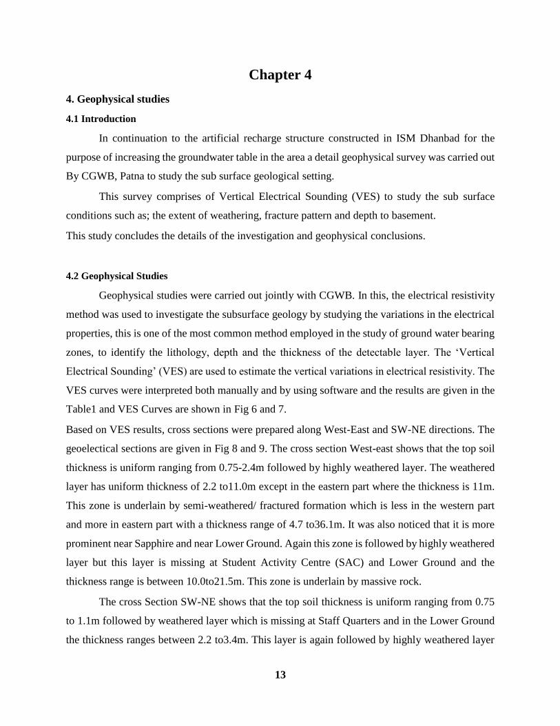
4.1 Introduction

In continuation to the artificial recharge structure constructed in ISM Dhanbad for the

purpose of increasing the groundwater table in the area a detail geophysical survey was carried out

By CGWB, Patna to study the sub surface geological setting.

This survey comprises of Vertical Electrical Sounding (VES) to study the sub surface

conditions such as; the extent of weathering, fracture pattern and depth to basement.

This study concludes the details of the investigation and geophysical conclusions.

4.2 Geophysical Studies

Geophysical studies were carried out jointly with CGWB. In this, the electrical resistivity

method was used to investigate the subsurface geology by studying the variations in the electrical

properties, this is one of the most common method employed in the study of ground water bearing

zones, to identify the lithology, depth and the thickness of the detectable layer. The ‘Vertical

Electrical Sounding’ (VES) are used to estimate the vertical variations in electrical resistivity. The

VES curves were interpreted both manually and by using software and the results are given in the

Table1 and VES Curves are shown in Fig 6 and 7.

Based on VES results, cross sections were prepared along West-East and SW-NE directions. The

geoelectical sections are given in Fig 8 and 9. The cross section West-east shows that the top soil

thickness is uniform ranging from 0.75-2.4m followed by highly weathered layer. The weathered

layer has uniform thickness of 2.2 to11.0m except in the eastern part where the thickness is 11m.

This zone is underlain by semi-weathered/ fractured formation which is less in the western part

and more in eastern part with a thickness range of 4.7 to36.1m. It was also noticed that it is more

prominent near Sapphire and near Lower Ground. Again this zone is followed by highly weathered

layer but this layer is missing at Student Activity Centre (SAC) and Lower Ground and the

thickness range is between 10.0to21.5m. This zone is underlain by massive rock.

The cross Section SW-NE shows that the top soil thickness is uniform ranging from 0.75

to 1.1m followed by weathered layer which is missing at Staff Quarters and in the Lower Ground

the thickness ranges between 2.2 to3.4m. This layer is again followed by highly weathered layer

14

which is uniform except near Teachers Colony where it is missing and the thickness range of this

is 8.9 to 16.3m. This zone is again underlain by semi-weathered or fractured formation which is

prominent in the NE part and is missing at Old Health Centre and the thickness range of this layer

is from 15.0 to 37.7m. This geophysical study concluded that the area is underlain by crystalline

metamorphic rocks of Archean age which forms the basement rock and enclaves of older

metamorphic rocks. The Groundwater is occurring in the phreatic conditions in the weathered zone

and under semi-confined conditions in the deep seated fractures of the rocks.

15

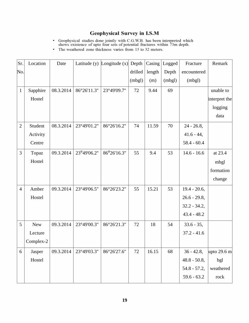
Table: 1 Results of VES Carried out in ISM campus

`

16

Fig: 5 Geophysical VES survey locations

Fig: 6 Vertical Electrical sounding curves at ISM campus

17

Fig: 7 Vertical Electrical sounding curves at ISM campus

18

Fig: 8 Geo-electrical Cross Section along West-east direction in ISM campus

Fig: 9 Geo-electrical Cross Section along SW-NE direction in ISM campus

19

Sr.

No.

Location Date Latitude (y) Longitude (x) Depth

drilled

(mbgl)

Casing

length

(m)

Logged

Depth

(mbgl)

Fracture

encountered

(mbgl)

Remark

1 Sapphire

Hostel

08.3.2014 86°26'11.3'' 23°49'09.7'' 72 9.44 69 unable to

interpret the

logging

data

2 Student

Activity

Centre

08.3.2014 23°49'01.2'' 86°26'16.2'' 74 11.59 70 24 - 26.8,

41.6 - 44,

58.4 - 60.4

3 Topaz

Hostel

09.3.2014 23⁰49'06.2'' 86⁰26'16.3'' 55 9.4 53 14.6 - 16.6 at 23.4

mbgl

formation

change

4 Amber

Hostel

09.3.2014 23°49'06.5'' 86°26'23.2'' 55 15.21 53 19.4 - 20.6,

26.6 - 29.8,

32.2 - 34.2,

43.4 - 48.2

5 New

Lecture

Complex-2

09.3.2014 23°49'00.3'' 86°26'21.3'' 72 18 54 33.6 - 35,

37.2 - 41.6

6 Jasper

Hostel

09.3.2014 23°49'03.3'' 86°26'27.6'' 72 16.15 68 36 - 42.8,

48.8 - 50.8,

54.8 - 57.2,

59.6 - 63.2

upto 29.6 m

bgl

weathered

rock

20

7 Staff

Quarters-2

(Behind

Dhurga

Mandir)

09.3.2014 23°48'43.1'' 86°26'15.1'' 72 15.25 70 19.6 - 21.2,

24.8 - 29.6,

30.8 - 32.4,

44 - 46.8

8 Diamond

Hostel

09.3.2014 23°48'55.9'' 86°26'27.4'' 72 15.24 35 upto 34 m

bgl highly

fracture

zone

9 SBI,

Govindpur

10.3.2014 70 19.8 66 32 - 36,

39.2 - 40.8

10 Shanti

Bhawan

10.3.2014 24°48'52.4'' 86°26'39.5'' 55.3 15.24 39 19 - 22.2,

34.6 - 36.4

Table: 2 Location showing the fractures encountered

Fig: 10 VES logs showing fractures at different depth

21

After the Geophysical studies, the selection of suitable site for recharge in ISM is done based on

the various factors;

• Availability of space for construction of recharge structures.

While preparing the recharge scheme, depth and shape of the storage facility in recharge structure

depends on:

-Availability of runoff

-Space availability in an area

It was observed by the ISM team that the recharge pits would be 10x30x10 (ft.) and is located in

open area that is distant from sewage structure and services. Previous studies done by Prof. R.K.

Verma and C.V. Rao in 1982 also shows that there is a fracture zone in the section A-A’ which is

plotted on graph. In his study he found that the weathered metamorphic layer whose resistivity

varies from 30to 80 ohm-m is found to be main aquifer. The thickness of the weathered layer is

about 8 to 45 meters. At some places semi weathered/fractured rocks under lie the weathered layer

and provide good aquifer conditions.

Fig: 11 Resistivity map of ISM, Verma and Rao, 1982

22

Chapter 5

5. Roof top Rain water Harvesting and Artificial Recharge

5.1 Rainwater harvesting

Rainwater harvesting is the techniques of collection and storing of rainwater for reuse

rainwater on-site, rather than allowing it to runoff. It is a process of arresting runoff water from

the roof tops and are let of into the outlets that are connected through a pipe to a storage tanks and

let into gravel filled trenches, pits to serve as recharge conduits. The uses of this recharge water

include gardening, livestock, irrigation and domestic use with proper treatment. Rainwater

harvesting systems can be installed with minimal skills. The system should be sized to meet the

water demand throughout the dry season since it must be big enough to support daily water

consumption. Specifically, the rainfall capturing area such as a building roof must be large enough

to maintain adequate flow. The water storage tank size should be large enough to contain the

captured water. Historically, this method is very old .In ancient Tamil Nadu (India), rainwater

harvesting was done by Chola Kings. Rainwater from the Brihadeeswarar temple was collected in

Shivaganga tank. During the later Chola period, the Viranam tank was built (1011 to 1037 CE) in

Cuddalore district of Tamil Nadu to store water for drinking and irrigation purposes. Viranam is a

16-kilometre (9.9 mi) long tank with a storage capacity of 1,465,000,000 cubic feet

(41,500,000 m3). Rainwater harvesting was done in the Indian states of Madhya

Pradesh, Maharashtra, and Chhattisgarh in the olden days. Ratanpur, in the state of Chhattisgarh,

had around 150 ponds. Most of the tanks or ponds were utilized in agriculture works. Recently in

Tamil Nadu, rainwater harvesting was made compulsory for every building to avoid ground water

depletion. It proved excellent results within five years, and every state took it as role model. Since

its implementation, Chennai saw a 50 per cent rise in water level in five years and the water quality

significantly improved. In Rajasthan, rainwater harvesting has traditionally been practiced by the

people of the Thar Desert. There are many ancient water harvesting systems in Rajasthan, which

have now been revived. Water harvesting systems are widely used in other areas of Rajasthan as

well, for example the chauka system from the Jaipur district. At present, in Pune (Maharashtra),

rainwater harvesting is compulsory for any new society to be registered. An attempt has been made

at Dept. of Chemical Engineering, IISc, Bengaluru to harvest rainwater using upper surface of a

solar still, which was used for water distillation.

23

In the context of ISM the Need for rainwater harvesting is because the surface water and other

water supply systems are slowly becoming inadequate to meet the demand here and have to depend

on ground water. This is happening due to rapid growth of the population in ISM also infiltration

of rain water into the sub-soil has decreased drastically and recharging of ground water has

diminished. So, to enhance the availability of ground water at ISM campus it became necessary to

raise the water level in wells and bore wells that are drying up. Also it helps in reduction of power

consumption and will improve the water quality in aquifers. Here, in ISM rain water is being

collected on the roofs of the building and from there it is being transported to the recharge pits

nearby which are constructed there.

5.2 Artificial Recharge:

Groundwater recharge or deep drainage or deep percolation is hydrologic process

where water moves downward from surface water to underground. This process usually occurs in

the vadose zone below plant roots and is often expressed as a Flux to the groundwater table surface.

Recharge occurs both naturally (through the water cycle) and through anthropogenic processes

(i.e., "artificial groundwater recharge"), where rainwater and /or reclaimed water is routed to the

subsurface. Artificial groundwater recharge is becoming increasingly in India. More pumping of

groundwater by farmers has led to underground resources becoming depleted. In 2007, on the

recommendations of the International Water Management Institute, the Indian government

allocated Rs.1800 crore (US$400million) of funds to dug-well recharge projects (a dug-well is a

wide, shallow well, often lined with concrete) in 100 districts within seven states where water

stored in hard-rock aquifers had been over-exploited.

Groundwater is recharged naturally by rain and snow melt and to a smaller extent by surface water

(rivers and lakes). Recharge may be impeded somewhat by human activities including paving,

development, or logging. These activities can result in loss of topsoil resulting in reduced water

infiltration, enhanced surface runoff and reduction in recharge. The volume-rate of abstract from

an aquifer in the long term should be less than or equal to the volume-rate that is recharged.

Recharge can help move excess salts that accumulate in the root zone to deeper soil layers,

or into the groundwater system. Tree roots increase the water saturation and reducing the

water runoff. Flooding temporarily increases river bed permeability by moving clay soils

downstream, and this increases aquifer recharge.

24

There are various artificial recharge techniques; flow chart shows the different types of it and the

marked one is the technique used in ISM.

Fig: 12 Different types of artificial recharge techniques

25

Fig: 13 Recharge pit Section

Fig: 14 Design of Recharge Pit in ISM.

26

Fig: 15 Dimensions of the recharge pit in ISM

5.3 Need for Augmentation of Groundwater Resources in I.S.M.

Augmentation of Ground water became very crucial in ISM because there was a sudden

increase of human population in the campus and there was high demand water expected due to

increase in new developmental works carried out in the campus. Also it became necessary to

efficiently manage the available resources as to meet the growing needs and demands adequately.

This conservation and augmentation has to follow appropriate means and also the effective route.

It was planned to be done by conservation and storage of surplus surface water run-off in

groundwater or sub-surface reservoirs in ISM campus and enhance the sustainable yield in the

ISM.

Other important reasons for need of artificial recharge were:

• Increased numbers of building in the campus due to development requirements.

• Improve the quality of existing groundwater through dilution.

• Save energy for lifting of groundwater from depleted level

• Decreasing area of open space or grass land which resulted in less water recharge and

increased the surface run off.

• Excessive ground water withdrawal.

27

• Decrease in infiltration due to decrease in open space area.

Fig. 16 shows the satellite view of the ISM campus and the rate of depletion of open grass land

which is affecting the water table.

Fig: 16 Satellite view of ISM, Dhanbad

28

Chapter 6

6. Ground Water Data Organization and Statistical Analysis

6.1 Data organization

Collection and collation of ground water data is a very important exercise and needs very

careful observation. The study covers a total area of 218 acres within the campus of Indian School

of Mines (ISM) situated in the Dhanbad, in the state of Jharkhand. There is a very high demand of

water as discussed in the previous chapters. To meet this demand, a project on “Rain Water

Harvesting and Artificial Recharge” proposed by ISM was sanctioned in August-2011 under

Central Sector Scheme “Ground Water Management and Regulation” in The State of Jharkhand

during XIth plan by the Central Ground Water Board (CGWB), Ministry of Water Resources for

implementation in the ISM campus. The project included construction of 54 recharge pits with

recharge bores along with connecting down pipes from rooftops and horizontal pipes to the

recharge pits. The constructions were to recharge the fractured aquifer system of the campus area.

The recharge pits of the dimension of 10ft x 3ft x 3ft are suitably placed at different locations

inside the campus with recharge bores, depth of which varies from 55m to 72 m and diameter of 4

inch. The recharge pits were located in an open areas near to buildings with roof top catchment

and are distant from sewage structures and services. Ground water level data were recorded from

the recharge bores in every month with the help of water level sounder. In this study, the

groundwater levels of pre-monsoon, monsoon and post-monsoon and fluctuation of pre-monsoon

and post-monsoon water levels were organized in a database, which were then analysed for

statistical and geostatistical study.

6.2 Statistical Analysis

Statistical Analysis of Groundwater table for Pre-monsoon, Monsoon, Post-monsoon and

Fluctuation for the year 2014 is shown in the table below.

29

Sr.

No.

Period Mean Range SD Skewness Kurtosis

Min Max

1. Pre-Monsoon(May-June) 240.652 225.874 246.140 3.922 -1.609 6.262

2. Monsoon(July-Aug-Sep) 242.124 227.804 246.865 3.870 -1.690 6.360

3. Post-Monsoon(Oct-Nov-Dec) 242.192 231.664 247.497 3.251 -1.068 4.678

4. Fluctuation Between Pre-

monsoon and Post-monsoon

1.862 0.045 8.715 1.407 2.703 13.228

Table: 3 statistics of groundwater in different periods of the year 2014

0

5

10

15

20

25

30

Fre

quen

cy

Class Interval

Fig: 17

Pre-Monsoon 2014

0

2

4

6

8

10

12

14

Fre

qu

ency

Class Interval

Fig:18

Monsoon 2014

0

5

10

15

20

25

Fre

quen

cy

Class Interval

Fig: 19

Post-monsoon 2014

0

5

1015

20

25

3035

Fre

quen

cy

Class Interval

Fig: 20

Fluctuation 2014

30

Fig: 20a Graph showing the pre-monsoon and post –monsoon groundwater level

215.0000

220.0000

225.0000

230.0000

235.0000

240.0000

245.0000

250.0000

Sap

hir

e H

ost

el

Sap

hir

e H

ost

el

Sap

hir

e H

ost

el

Sap

hir

e H

ost

el

Sap

hir

e H

ost

el

Sap

hir

e H

ost

el

Top

az H

ost

el

Top

az H

ost

el

Stu

de

nt

Act

ivit

y C

entr

e

Stu

de

nt

Act

ivit

y C

entr

e

Stu

de

nt

Act

ivit

y C

entr

e

Am

ber

Ho

stel

Am

ber

Ho

stel

Am

ber

Ho

stel

Am

ber

Ho

stel

Bac

k Si

de

of

Emer

ald

Ho

ste

l p

it

Bac

k Si

de

of

Emer

ald

Ho

ste

l p

it

Fro

nt

Sid

e o

f Em

eral

d H

ost

el p

it

Fro

nt

Sid

e o

f Em

eral

d H

ost

el p

it

Jasp

er H

ost

el

Jasp

er H

ost

el

Jasp

er H

ost

el

Her

itag

e B

uild

ing

Dia

mo

nd

Ho

ste

l

Op

al H

ost

el

Op

al H

ost

el

Op

al H

ost

el

Op

al H

ost

el

Old

Lib

rary

Pet

role

um Sh

anti

Bh

awan

Haw

a M

ahal

Haw

a M

ahal

Wo

rk s

ho

p &

MM

E

Sta

ff C

olo

ny

Typ

e II

,

Sta

ff C

olo

ny

Typ

e II

,

Low

er g

rou

nd

Lect

ure

hal

l co

mp

lex

II

Lect

ure

hal

l co

mp

lex

II

Hea

lth

Cen

tre

(old

)

Teac

her

s co

lon

y

Teac

her

s co

lon

y

SBI B

ank

ISM

SBI B

ank

ISM

Gro

und w

ater

tab

le D

epth

Location

Groundwater Table in Pre and Post- monsoon 2014

Pre-monsoon 2014 Post-monsoon 2014

31

Fig: 20b Graph showing the pre-monsoon and post –monsoon groundwater

0

1

2

3

4

5

6

7

8

9

10

Sap

hir

e H

ost

el

Sap

hir

e H

ost

el

Sap

hir

e H

ost

el

Sap

hir

e H

ost

el

Sap

hir

e H

ost

el

Sap

hir

e H

ost

el

Top

az H

ost

el

Top

az H

ost

el

Stu

de

nt

Act

ivit

y C

entr

e

Stu

de

nt

Act

ivit

y C

entr

e

Stu

de

nt

Act

ivit

y C

entr

e

Am

ber

Ho

stel

Am

ber

Ho

stel

Am

ber

Ho

stel

Am

ber

Ho

stel

Bac

k Si

de

of

Emer

ald

Ho

ste

l p

it

Bac

k Si

de

of

Emer

ald

Ho

ste

l p

it

Fro

nt

Sid

e o

f Em

eral

d H

ost

el p

it

Fro

nt

Sid

e o

f Em

eral

d H

ost

el p

it

Jasp

er H

ost

el

Jasp

er H

ost

el

Jasp

er H

ost

el

Her

itag

e B

uild

ing

Dia

mo

nd

Ho

ste

l

Op

al H

ost

el

Op

al H

ost

el

Op

al H

ost

el

Op

al H

ost

el

Old

Lib

rary

Pet

role

um Sh

anti

Bh

awan

Haw

a M

ahal

Haw

a M

ahal

Wo

rk s

ho

p &

MM

E

Sta

ff C

olo

ny

Typ

e II

,

Sta

ff C

olo

ny

Typ

e II

,

Low

er g

rou

nd

Lect

ure

hal

l co

mp

lex

II

Lect

ure

hal

l co

mp

lex

II

Hea

lth

Cen

tre

(old

)

Teac

her

s co

lon

y

Teac

her

s co

lon

y

SBI B

ank

ISM

SBI B

ank

ISM

Flu

ctu

atio

n in

Met

er

Location

Fluctuation 2014

32

6.3 Discussion

The minimum and maximum values for pre-monsoon has a mean of 240.652 and standard

deviation (SD) of 3.922 giving a co-efficient of variation (SD/mean) 61.35 which is very high. The

skewenss value is -1.609, it is very high and negatively skewed (Fig 17). Kurtosis value is 6.262

and is in the range of lepto-kurtic since it is more than 3and thus it is non-normal distribution. The

Table-3 gives the statistical values for all pre-monsoon, monsoon, post-monsoon and fluctuation

which are different for all but the character of the three periods are all same leaving the fluctuation.

The parameters showed that the value range is beyond 7 confirming it to be log-normal

distribution. The figure17-19 showing the log-normal distribution of groundwater.

33

Chapter 7

7. Geostatistical Modelling of Ground Water Resource

7.1 Introduction

In this part Geostatistical modelling is carried out with semivariography i.e.

characterization of spatial distribution of groundwater. A semivariogram model exhibit various

characteristics that display spatial distribution parameters i.e. Nugget effect (C0), Continuity (C),

range of influence (a) and anisotropy. To investigate the seasonal variation in both the season i.e.

pre-monsoon and post-monsoon and to model the fluctuation of ground water table in and around

ISM Dhanbad, geostatistical method is used. The methods adopted is to study the spatial

distribution of groundwater table in the ISM campus and to generate the ground water distribution

maps. Since the area is a hard rock terrain the major aquifer system is in fractured zones and the

basement rock with shallow fractures generally encountered at various depths ranging from 10 to

70 meters. There are different fractured zones and each zone has different thickness. Groundwater

level data were collected in 48 wells during pre-monsoon, in 34 wells during monsoon and in 54

wells during post-monsoon periods in the year 2014. The data were collected manually and then

processed for statistical and geostatistical analysis. The entire one year data of 2014 were divided

in to pre-monsoon, monsoon and post-monsoon in which the pre-monsoon consists of the average

water table of May-June, monsoon consists of average water table of July-August-September and

Post-monsoon consists of the average water table of October-November-December. For the study

of fluctuation, the difference of water table depth of pre-monsoon and post-monsoon was

calculated which is given in Table 4.

Location Name

Pre-

monsoon

Post-

monsoon Fluctuation

Sapphire Hostel 243.6189 244.0339 0.4150

Sapphire Hostel 242.8900 243.8900 1.0000

Sapphire Hostel 243.7339 244.5089 0.7750

Sapphire Hostel 242.3889 243.2989 0.9100

Sapphire Hostel 242.2067 242.9667 0.7600

Sapphire Hostel 246.1406 246.5906 0.4500

34

Topaz Hostel 242.0103 242.8253 0.8150

Topaz Hostel 243.7641 244.2791 0.5150

Student Activity Centre 241.4003 242.4453 1.0450

Student Activity Centre 240.7636 242.4636 1.7000

Student Activity Centre 239.2210 242.3860 3.1650

Amber Hostel 243.8109 245.4259 1.6150

Amber Hostel 243.6751 245.6701 1.9950

Amber Hostel 243.8572 245.2472 1.3900

Amber Hostel 238.3111 239.5161 1.2050

Back Side of Emerald Hostel 243.8713 245.4163 1.5450

Back Side of Emerald Hostel 243.8230 245.3680 1.5450

Front Side of Emerald Hostel 244.9946 246.5146 1.5200

Front Side of Emerald Hostel 244.2362 245.2062 0.9700

Jasper Hostel 237.6016 237.9966 0.3950

Jasper Hostel 239.3737 240.8937 1.5200

Jasper Hostel 242.4050 244.3250 1.9200

Heritage Building 240.7042 242.2392 1.5350

Diamond Hostel 243.1233 244.7933 1.6700

Opal Hostel 241.0454 244.2804 3.2350

Opal Hostel 245.2572 247.4972 2.2400

Opal Hostel 240.8138 243.7738 2.9600

Opal Hostel 241.5937 243.9087 2.3150

Old Library 239.2508 241.7908 2.5400

Petroleum 229.3721 231.8121 2.4400

Shanti Bhawan 236.3884 238.7684 2.3800

Hawa Mahal 236.6502 238.8152 2.1650

Hawa Mahal 236.4069 238.9369 2.5300

Work shop & MME 241.8070 241.8520 0.0450

35

Staff Colony Type II, 236.9900 239.4000 2.4100

Staff Colony Type II, 236.9903 238.2853 1.2950

Lower ground 238.1001 240.0951 1.9950

Lecture hall complex II 241.8707 243.1557 1.2850

Lecture hall complex II 239.7728 242.1878 2.4150

Health Centre (old) 238.2449 240.4249 2.1800

Teachers colony 225.8745 231.6645 5.7900

Teachers colony 233.4261 242.1411 8.7150

SBI Bank ISM 244.7678 246.7928 2.0250

SBI Bank ISM 241.4679 244.0429 2.5750

Table: 4 Groundwater Table data

7.2 Semi-variography

Point kriging

Point kriging is a method of estimation or interpolation of a point by a set of neighbouring

sample points applying the theory of regionlized variables where the sum of weight coefficients

sum to unity and produce a minimum variance of error.

Expressed mathematically, kriged estimate is given as-

P*=∑aisi

Where P*= the estimate of true value sat a point ‘p’

ai= weight coefficient of the individual samples

si= individual sample values at sample points, si.

And kriging variance is given by

𝝈k2=∑ ai𝜸(si,p)+ λ

Where, λ= Lagrangian multiplier and 𝛾(si, p) = average semi-variance among samples and the

point to be estimate.

36

According to David (1977) point kriging is a procedure for checking the validity of a

semivariogram model that represents the underlined semivariograms. A spherical model is fitted

to an experimental semivariogram by adjusting C0 (Nugget effect), C (Continuity) and a (range).

To understand the anisotropy of the fluctuations and level of groundwater table during pre and

post monsoon, comparison of variograms with experimental semivariograms to cross validate

with the model was done. During this procedure, since the sample points are randomly distributed,

different lag distance and sample interval was taken to fit the spherical model ( Fig: 21,22,23 )

These models were Cross validated with Point Kriging Cross Validation Technique and were fitted

to the experimental semi-variogram models. The Point kriging cross validation was done by

selecting the most suitable range, nugget, continuity and keeping the sill value at the most suitable

place so that maximum points can be covered and best fit can be obtained

Cross-validated models as obtained employing Point kriging cross-validation technique for

Pre-monsoon, Post-monsoon, and Fluctuation given in Figure 21, 22, and 23 and the analysis of

the point kriging cross validation are given in Table 6, 7 and 8 respectively.

0 500 1000 1500

0

5

10

15

20

25

30

35

40

C0

+C

Lag (m)

Fig: 21 Experimental semivariogram with fitted model for Pre-Monsoon period

37

0 200 400 600 800 1000 1200

0

10

20C

0+

C

LAG (m)

Fig: 22 Experimental semivariogram with fitted model for Post-Monsoon period

0 200 400 600 800 1000 1200 1400 1600 1800 2000

0

1

2

3

4

5

6

C0

+C

Lag (m)

Fig: 23 Experimental semivariogram with fitted model for Fluctuation

38

Sr. No. Period Model

1. Pre-monsoon γ(h)= 3.0+23[(1.5xh/875)-1.5(h/875)3]

2. Post-monsoon γ(h)= 3.8+10[(1.5xh/600)-1.5(h/600)3]

3. Fluctuation γ(h)= 0.7+1.40[(1.5xh/800)-1.5(h/800)3]

Table: 5 Model selected for Kriging for different periods

Variogram models were cross validated by taking the various lag distances as the sample

distance were randomly distributed and to get the best fitted model the exercise was carried out

Table 6, 7 and 8 gives the details of the exercise and various values for fulfilling the parameters.

Semi

Variogram Parameters

Initial Parameter values Final

Values

C0 2.0 2.6 2.6 2.6 2.7 3.0 4 3.0 3.0

C 19 22 21.6 22 22 22 21 22 23

C0+C 21 24.6 24.6 24.6 24.7 25 25 25 26

Range(a) 900 750 750 800 750 850 800 875 875

KE:EV 1.43 1.07 1.08 1.10 1.04 1.04 0.87 1.05 1.03

Table: 6 Initial and Final parameter values of Point kriging cross validation process for Pre-

monsoon 2014

Semi

Variogram

Parameters

Initial Parameter values Final

Values

C0 3.41 3.40 3.41 3.41 3.41 3.4 3.4 3.4 3.8

C 12.0 12.1 12.0 12.0 12.0 10.5 11.0 10.5 10.0

C0+C 15.41 15.51 15.41 15.41 15.41 13.9 14.4 13.9 13.8

Range(a) 1000 1050 800 700 600 600 800 500 600

KE:EV 1.20 1.22 1.14 1.09 1.05 1.09 1.17 1.05 1.02

Table: 7 Table: 6 Initial and Final parameter values of Point kriging cross validation process for

Post-monsoon 2014

39

Semi

Variogram Parameters

Initial Parameter values Final

Values

C0 0.32 0.50 0.6 0.5 0.55 0.4 0.55 0.6 0.7

C 1.98 1.5 1.4 1.4 1.35 1.65 1.60 1.45 1.40

C0+C 2.3 2 2 1.9 1.9 2.05 2.15 2.05 2.1

Range(a) 800 650 650 650 650 700 670 700 800

KE:EV 1.30 1.08 1.02 1.04 1.08 1.04 1.02 1.04 1.04

Table: 8 Table: 6 Initial and Final parameter values of Point kriging cross validation process for

fluctuation of Pre and Post 2014

It can be observed that in pre monsoon and post monsoon the nugget is 3.0 and 3.8 but in

the fluctuation case the nugget goes to 1.40 which is almost half of the pre and post monsoon.

Therefore, the accuracy of the Kriged values depends on the variogram values at most possible

small lag distances (Isaaks & Srivastava, 1989) and the fig 21. Clearly demonstrates that first few

points associated to lag distance carry more weights of spatial structure (Ma et al., 1999).

7.3 Block Grids Delineation

Kriging

The geostatistical procedure of estimating values of a regionalized variable using the

information obtained from a semi-variogram is kriging. Its application to groundwater hydrology

has been described by number of authors, viz. Delhomme(1976,1978,1979), Delfiner and

Delhomme(1953),Marsily et al. (1984), Marsily (1986),Aboufirassi and Marino(1983,1984),

Gambolti and Volpi (1979) to name a few.

Let G* be the kriged estimate of the average value of grid G of the samples having values g1, g2,

g3……gn. Let a1, a2, a3……an be the weightage giving to each of the values respectively such that

∑ai=1; and G*=∑aigi. Thus the estimation becomes unbiased; the mean error is zero for a large

40

number of estimated values and the estimated variance is minimum. The kriging variance is given

as

𝛔𝐤𝟐 = ∑(𝐠𝐢 − 𝐆∗)2

To make kriging variance minimum, a function called Lagrange multiplier (λ), is used for

optimal solution of the kriging system. Kriging carried out for a point estimate is called point

kriging and that accomplished for making estimates of a block of ground is known as block kriging.

The kriging technique is applied for analytical purpose and is discussed below.

Prior to kriging the block size of the study area was decided by taking into account the

various parameters i.e. area, fluctuation of ground water and the best fitted block which can cover

the maximum extent near to the boundary of the ISM. Since area is small and is heterogeneously

extended from all direction here, 25m x 25m x 25m dimensions of the block size was delineated

after a number of exercises so that kriging can be done for whole area. After the delineation of the

block grid of the dimension 25m x 25m x 25m the center points of each block was taken and the

kriging technique was applied.

7.4 Ordinary Kriging

Here Ordinary Kriging was applied for the estimation of the fluctuation of groundwater

table across the area and to delineate the groundwater table structure of pre and post monsoon.

Since kriging is a geostatistical interpolation technique which considers both distance and degree

of variation between known and estimated values. This method is an attempt to minimize the error

variance and set the mean of the prediction error to zero so that there is no over or under estimates

as it is a robust interpolation technique which derives weights from surrounding measured values

to predict values at unmeasured locations.

The figures shows the spatial distribution of groundwater developed across the study area.

The figure of pre-monsoon (fig. 24) and post-monsoon (fig. 25) shows the amount of Kriged

groundwater table and the third is the amount of fluctuation (fig. 26) across the area and fig. 27,

28, 29 shows the Standard deviation (Error) associated with the estimation of the groundwater

table. Fig.24 shows the distribution of ground water table during the pre-monsoon period. In this

map it can be seen that the water table towards the NW side of the area is at a higher level and

41

towards NE side is at a deeper level, this also confirms the topographical elevation of the area

which is also similar to this and dependence of the groundwater table on the topographical

elevation . The NW side has a higher elevation and NE is at a lower elevation. When compared

this map with Post-monsoon Kriged map it can be seen that the recharge pits have shown a positive

trend and the Kriged Map shows, the fluctuation in water level is taking place due to rise in

groundwater table.

42

Fig: 24 Kriged Estimate distribution map of Pre-monsoon groundwater level

43

Fig: 25 Kriged Estimate distribution map of Post-monsoon groundwater level

44

Fig: 26 Kriged Estimate distribution map of Fluctuation of groundwater level

45

Fig: 27 Kriged SD map of Pre-monsoon Groundwater level

46

Fig: 28 Kriged SD map of Post-monsoon Groundwater level

47

Fig: 29 Kriged SD map of Fluctuation Groundwater level

.

48

7.5 Results and Discussion

From the Kriged Estimate Fluctuation map it can be noticed that the NW (0.78m) part is

having the least rise in water table than the NE (5.3m) part. NE part having high fluctuation also

highlights that the draft being done by the pump house which is pumping out the water at regular

interval and it shows a depression structure being developed there. Furthermore it is observed that

the kriged standard deviation (error) map shows that the error associated with the Kriged estimate

in all the three maps. The KSD map shows that the maximum error is at the NE side where the

water is being drafted regularly and the depression is getting created also in the fluctuation KSD

map .The red zone are showing the maximum error and the dark blue is showing the minimum.

This also confirms that the recharge pits located at the Northern and NW part of the study area is

controls the error. Furthermore it can be seen where ever the recharge pits are present the error is

less and it gradually increases when moved away from the recharge pit.

To study the flow direction of the groundwater during different period, different contour

maps were developed on the Kriged surfaces to visualize and simulate the groundwater scenario

in the subsurface region of the ISM campus. The figures from 30 to 35 shows and gives the

direction of flow of subsurface water during the pre-monsoon and post-monsoon periods. It can be

noticed that there is not much difference in the flow direction and is following the topographic

elevation system.

The water table contour map from figure 30 to 35, it can be observed that the flow direction

is from NW to NE and SW divergence can also be observed in the central ridge portion i.e.

topographically controlled groundwater flow. In the north eastern part a groundwater trough with

central flow is noticed from the spacing of the water table contour map. A generalized estimate of

the hydraulic characteristics can also be made.

There is higher transitivity of the fractured aquifers which are indicated by the

comparatively larger spacing in the contour lines of the NW, Western and South Western part of

the campus.

49

Fig: 30 Kriged estimate contour map of Pre-monsoon groundwater table

Fig: 31 Kriged estimate contour map of Post-monsoon groundwater table

50

Fig: 32 Kriged estimate contour map of Fluctuation in groundwater table

Fig: 33 Kriged SD contour map of Pre-monsoon groundwater table

51

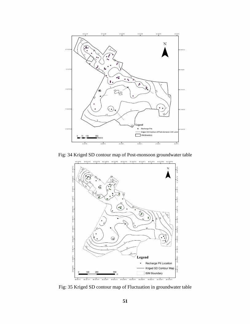
Fig: 34 Kriged SD contour map of Post-monsoon groundwater table

Fig: 35 Kriged SD contour map of Fluctuation in groundwater table

52

It can be seen that the level of water table is higher in the NW part than the NE part. It can

also be visualized that the flow of ground water is moving out of the ISM when we see from the

center of the map and there is a development of ridge like structure which is controlling it, when

we compare this with the topographic elevation of the area it can be verified that the center part

i.e. The Heritage Building and surrounding are at a higher elevation i.e. from there the ground

water is flowing out of the campus towards the SW and also towards the NE part of the area where

the depression is being created.

Mean of the

actual and

estimated=0.002

R=0.9373

Fig: 36 Regression line of pre-monsoon

In order to verify the accuracy of the variogram models fitted, that was used to estimate

the groundwater table for all the three pre, post and fluctuation of the figures 36, 37 and 38 shows

the graph and the regression line between the observed and the estimated values of ground water

table during the pre-monsoon and post-monsoon period and of the fluctuation. The above graphs

shows the R values of Pre-post and fluctuation which are 0.937, 0.871 and 0.877 respectively. The

mean of the actual to that of estimated (i.e. 0.002, 0.005, 0.004) is also reliable and supporting the

unbiasedness constraint of Kriging (Goovaerts, 1997).

y = 0.7625x + 57.166

R² = 0.8787

228

230

232

234

236

238

240

242

244

246

248

220 225 230 235 240 245 250

Est

imat

ed V

alues

Measured Values (m)

Kriged Estimate Premonsoon

53

Mean of the

actual and

estimated=0.005

R=0.871

Fig: 37 Regression line of post-monsoon

Mean of the

actual and

estimated=0.004

R=0.877

Fig: 38 Regression line of fluctuation

y = 0.6107x + 94.288

R² = 0.7603

234

236

238

240

242

244

246

248

230 235 240 245 250 255

Est

imat

ed V

alu

es (

m)

Measured Values (m)

Kriged Estimate Postmonsoon

y = 0.6049x + 0.7706

R² = 0.7757

0

1

2

3

4

5

6

7

8

0 2 4 6 8 10 12

Est

imat

ed V

alues

(m

)

Measured Values (m)

Kriged Estimate of Fluctuation

54

However a little bias can be seen from the slope so ‘t’ on ‘r’ test were performed to determine the

significance of ‘r’ for all pre, post and fluctuation, the ‘t’ test was performed separately and was

found that the ‘r’ is significant in all the cases. The calculation is described below.

For Pre-monsoon

‘t’calc on ‘r’ = 𝒓√𝒏−𝟐

√𝟏−𝒓𝟐 = 18.40

‘t’table (α=0.05, ν=n-2, q=1-α) = 1.68

(i) If tcalc ≤ ttable : H0 is accepted and r is insignificant

(ii) If tcalc ≥ ttable : H1 is accepted and r is significant

For Post Monsoon

‘t’calc on ‘r’ = 𝒓√𝒏−𝟐

√𝟏−𝒓𝟐 = 12.80

‘t’table (α=0.05, ν=n-2, q=1-α) = 1.67

(i) If tcalc ≤ ttable : H0 is accepted and r is insignificant

(ii) If tcalc ≥ ttable : H1 is accepted and r is significant

For Fluctuation

‘t’calc on ‘r’ = 𝒓√𝒏−𝟐

√𝟏−𝒓𝟐 = 11.90

‘t’table (α=0.05, ν=n-2, q=1-α) = 1.68

(i) If tcalc ≤ ttable : H0 is accepted and r is insignificant

(ii) If tcalc ≥ ttable : H1 is accepted and r is significant

55

Chapter 8

8. Groundwater Resource Assessment

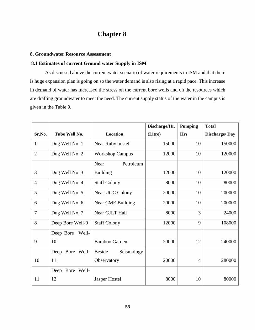
8.1 Estimates of current Ground water Supply in ISM

As discussed above the current water scenario of water requirements in ISM and that there

is huge expansion plan is going on so the water demand is also rising at a rapid pace. This increase

in demand of water has increased the stress on the current bore wells and on the resources which

are drafting groundwater to meet the need. The current supply status of the water in the campus is

given in the Table 9.

Sr.No. Tube Well No. Location

Discharge/Hr.

(Litre)

Pumping

Hrs

Total

Discharge/ Day

1 Dug Well No. 1 Near Ruby hostel 15000 10 150000

2 Dug Well No. 2 Workshop Campus 12000 10 120000

3 Dug Well No. 3

Near Petroleum

Building 12000 10 120000

4 Dug Well No. 4 Staff Colony 8000 10 80000

5 Dug Well No. 5 Near UGC Colony 20000 10 200000

6 Dug Well No. 6 Near CME Building 20000 10 200000

7 Dug Well No. 7 Near GJLT Hall 8000 3 24000

8 Deep Bore Well-9 Staff Colony 12000 9 108000

9

Deep Bore Well-

10 Bamboo Garden 20000 12 240000

10

Deep Bore Well-

11

Beside Seismology

Observatory 20000 14 280000

11

Deep Bore Well-

12 Jasper Hostel 8000 10 80000

56

12

Deep Bore Well-

13 In Front Of Old EDC 8000 10 80000

13

Deep Bore Well-

14

SBI ISM Campus

Branch 8000 12 96000

14

Deep Bore Well-

15

Beside 150 Quarters GR

Side 8000 12 96000

15

Deep Bore Well-

16

EDC Extension

Building 8000 10 80000

Total 1954000

Total Consumption / Month 1954000x30= 58620000

Table: 9 pumping of groundwater in ISM

Here it can be seen that seven dug wells and eight tube wells are supplying 1954000 liters

per day but still ISM purchases 850000 liters per day from D.W. &S department to meet the

demand and pays a high amount of money. Also the depth of water table has a high impact on

pumping out as when the water table is at high depth the electricity consumed is more and the

energy needed is more which ultimately increases the cost of the water. The current energy

consumption status of ISM is given in Table 10.

Sr.No. Tube Well No. Location

HP

Rating

Pumping

Hrs /Day

Units

Cosumed/Day

1 Dug Well No. 1 Near Ruby hostel 7.5 10 55.95

2 Dug Well No. 2 Workshop Campus 7.5 10 55.95

3 Dug Well No. 3 Near Petroleum Building 15 10 111.90

4 Dug Well No. 4 Staff Colony 7.5 10 55.95

5 Dug Well No. 5 Near UGC Colony 15 10 111.90

6 Dug Well No. 6 Near CME Building 15 10 111.90

57

7 Dug Well No. 7 Near GJLT Hall 5 3 11.19

8 Deep Bore Well-9 Staff Colony 7.5 9 50.36

9 Deep Bore Well-10 Bamboo Garden 15 12 134.28

10 Deep Bore Well-11

Beside Seismology

Observatory 7.5 14 78.33

11 Deep Bore Well-12 Jasper Hostel 5 10 37.30

12 Deep Bore Well-13 In Front Of Old EDC 5 10 37.30

13 Deep Bore Well-14 SBI ISM Campus Branch 5 12 44.76

14 Deep Bore Well-15

Beside 150 Quarters GR

Side 5 12 44.76

15 Deep Bore Well-16 EDC Extension Building 5 10 37.30

Total 979.13

Total Consumption / Month 979.13x30 = 29373.90

Table: 10 Units consumed for drafting groundwater in ISM

When we calculate it yearly the water discharge from the ground water is 21.39 mcm and

the total expense of drafting this water comes around 1.07 million units which costs very heavy

amount, financially and also it generates heavy load on the energy point of view. To curtail down

this and to convert the ground water cheaper the best way is to decrease the water table depth

which has direct effect on the energy consumption. Also these artificial structures to recharge the

groundwater table has very long term effect and it can be very beneficial not to ISM but also to

the surrounding area. Moreover it has been observed in the surrounding area the old dug wells

which used to be dry during summers has water of about 1m in them and did not dried up.

8.2 Groundwater Resources Estimation Methodology

Ground Water Resource Estimation Methodology – 1997 (GEC’97) recommends two approaches

for groundwater assessment– (i) water level fluctuation method and (ii) norms of rainfall infiltration

method.

The water level fluctuation method is based on the concept of storage change due to difference

between various input and output components (application of groundwater balance equation). The input

58

refers to recharge from rainfall and other sources and subsurface inflow into the unit of assessment. Output

refers to the groundwater draft, groundwater evapotranspiration, and base-flow to streams and subsurface

outflow from the unit. Since the data on subsurface inflow/ outflow are not readily available, it is

advantageous to adopt the unit for groundwater assessment as basin/ sub-basin/ watershed, as the inflow /

outflow across these boundaries may be taken as negligible.

Thus, the groundwater resource assessment unit is in general watershed particularly in hard

rock areas where as in case of alluvium areas, administrative block can also be the assessment unit.

In each assessment unit, hilly areas (areas having slope greater than 20%) are to be identified and

deducted from the total geographical area as these are not likely to contribute to groundwater

recharge. Further, areas where the quality of groundwater is beyond the permissible limits for

irrigation purposes should also be identified and assessment should be made separately. The

remaining area after deleting the hilly area and separating the area with poor groundwater quality

is to be delineated into command and non-command areas. Ground water assessment in command

and non-command areas are done separately for both the monsoon and the non-monsoon seasons.

8.3 Groundwater Recharge

8.3.1 Monsoon season

The resource assessment during monsoon season is estimated as the sum total of the change in

storage and gross draft. The change in storage is computed by multiplying water level fluctuation between

pre- and post-monsoon periods with the area of assessment and specific yield. Monsoon recharge can be

expressed as -

R = (h x Sy x A) + DG

Where,

h = rise in water level in the monsoon season,

A = area for computation of recharge,

Sy = specific yield,

DG = gross groundwater draft

The monsoon groundwater recharge has two components – rainfall recharge and recharge from other

sources. Mathematically it can be represented as –

59

R (Normal) = Rrf (normal) + Rc + Rsw + Rt + Rgw + Rwc

Where, Rrf is the normal monsoon rainfall recharge. The other sources of groundwater recharge during

monsoon season include Rc, Rsw, Rt, Rgw, Rwc which are recharge from rainfall, seepage from canals, surface

water irrigation, tanks and ponds, groundwater irrigation, water conservation structures respectively.

The rainfall recharge during monsoon season computed by Water Level Fluctuation (WLF)

method is compared with recharge estimated by Rainfall Infiltration Factor (RIF) method based on rainfall

infiltration factor. In case if the difference between the two sets of data are more than +20% , 1.2 times the

value estimated by RIF method is taken and if the difference is less than -20%, then 0.8 times the value

estimated by RIF method is taken. In case, the difference between the two sets of data remains between

+20% and -20%, monsoon recharge from water level fluctuation (WLF) is adopted.

8.3.2 Non-Monsoon season

Rainfall recharge is computed by using Rainfall Infiltration Factor (RIF) method during non-

Monsoon season. Recharge from other sources is then added to get total non-Monsoon recharge. In case of

areas receiving less than 10% of the annual rainfall during non-monsoon season, the recharge due to rainfall

may be taken as zero.

Total annual groundwater recharge

The total annual groundwater recharge of the area is the sum-total of monsoon and non-monsoon

recharge. An allowance is kept for natural discharge during non-monsoon season by deducting 5% of total

annual groundwater recharge, if WLF method is employed to compute rainfall recharge during monsoon

season and 10% of total annual groundwater recharge if RIF method is employed. The balance groundwater

available accounts for existing groundwater withdrawal for various uses and potential for future

development. This quantity is termed as Net Ground Water Availability.

Net Ground Water Availability = Annual Ground Water – Natural discharge during non-

Recharge monsoon season

An attempt has been made to estimate the replenishable groundwater resource within the campus

using the norms of Ground Water Resource Estimation (GEC 1997) methodology with the help of

60

Kriged estimate of the fluctuation of the groundwater table. The volume is calculated from the mean Kriged

value of the fluctuation of the entire area.

The total replenishable volume of water or dynamic groundwater resource is calculated by the below

formulae

Volume of water recharge = (Area x fluctuation x 0.03) + Total draft during the period

Here, 0.03 is the specific yield considered for hard rock as per GEC, 1997

Hence, (60 x 56 x 25 x 25 x 2.29 x 0.03 = 144270 m3) + Total Draft

The volume of water recharged is 144270 m3 x 1000 = 144,270,000 liters

As given in Table 9 the draft related to consumption from ground water for the study period is 19,54,000 x

12 x 30 = 703,440,000liters and as calculated the recharge volume in groundwater above the excess water

used can be calculated from the subsurface

703,440,000 + 144,270,000 = 847,710,000 liters

Here it can be seen that about 83% of total volume of water available is being used and still the

campus area is surplus of groundwater which is around 17%.It should also be noted that this much of draft

is sustainable and can be calculated only when this study is continued by collecting more data in the coming

years and then only the trend of the groundwater table can be developed which will be key to predict the

groundwater fluctuation in the long run. By observing the current data water consumption and correlating

by collecting the same in future and further studies can reveal more accurate and effect of these recharge

pits.

8.3.3 Norms for Estimation of Recharge

GEC’97 methodology has recommended norms for various parameters being used in groundwater

recharge estimation. These norms vary depending upon water bearing formations and agro-climatic

conditions. While norms for specific yield and recharge from rainfall values are to be adopted within the

guidelines of GEC’97, in case of other parameters like seepage from canals, return flow from irrigation,

recharge from tanks & ponds, water conservation structures, results of specific case studies may replace the

adhoc norms.

61

8.4 Ground Water Draft

The gross yearly groundwater draft is to be calculated for irrigation, domestic and industrial uses.

The gross groundwater draft would include the groundwater extraction from all existing groundwater

structures during monsoon as well as during non-monsoon period. While the number of groundwater

structures should preferably be based on latest well census, the average unit draft from different types of

structures should be based on specific studies or ad-hoc norms given in GEC’97 report.

62

Chapter 9

9. Groundwater Quality in ISM

9.1 Chemical analysis of groundwater

The importance of ground water quality has become increasingly recognized as

development of ground water continues to expand in British Columbia. Monitoring of ground

water quality is becoming more important because of contamination concerns and development of

new equipment and techniques for measuring contaminants in minute concentrations.

Although ground water is generally less susceptible to contamination than surface waters it is

usually more highly mineralized in its natural state. As water moves slowly through the ground it

can remain for extended periods of time in contact with minerals present in the soil and bedrock

and become saturated with dissolved solids from these minerals. This dissolution process continues

until chemical equilibrium is reached between the water and the minerals with which it is in

contact. The types and relative concentrations of the chemical constituents in ground water provide

information on the evolution of ground waters, age (residence time), and solubility, rates of

movement, flow history and sources of recharge. Older ground waters for example are generally

more mineralized than younger ground waters. Fresher ground waters are normally associated with

recharge areas whereas ground waters in discharge areas are more mineralized. Ground waters can

be classified according to the most dominant percentage of cations and anions being present based

on concentrations in equivalents per million [epm] (e.g., calcium-magnesium bicarbonate type).

9.2 Hydro chemical findings in ISM campus

The groundwater of the study area is mildly alkaline in nature with average pH value of

7.95. No sample contains carbonate but are characterised by the presence of bi-carbonate. The

maximum concentration of HCO3 was found as 344 mg l-1.

The value of electrical conductivity (EC) is from 202 to 1206 µS Cm-1 at 25oC which indicates a

wide variation in dissolved constituents.

63

In general, the quality of groundwater in terms of Total Hardness as CaCO3 has been found as

moderately hard to very hard. The maximum concentration of Ca has been found as 176 mg/L

and that is of Mg has been observed as 74 mg/L.

The concentration of Na ranged from 13 mg/L to 59 mg/L with an average of 40 mg/l and K was

found in the range from 1 mg/L to 9 mg/L with an average of 03 mg/L.

The concentration of Chloride in all of the ground water samples has been found to be within the

desirable limit for drinking purpose by BIS 2012. The maximum concentration of chloride has

been found as 163 mg/L. None of the analyzed sample showed Nitrate concentration higher than

the permissible limit of 45 mg/L and ranged from traces to 43 mg/L.

Concentration of Sulphate ion ranged from 8 to 110 mg/L. Fluoride ion concentration varied

from Traces to 1.19 mg/L with an average value of 0.41 mg/L. Phosphate has not been detected

from any of the sample. The silicate concentration was in the range of Traces to 17 mg/L.

As per the Na% value, Residual Sodium Carbonate and Sodium Adsorption Ratio all the analyzed

samples have been found safe and of excellent category.

Mostly no major threat has been identified according to analyzed major parameters from drinking

water perspective (Drinking water specification: BIS, 2012). All the analyzed samples have also

been found suitable for use in irrigation and allied purposes.

64

No. of Samples = 15

Parameters BIS Permissible Limit* in absence of alternate

source

No. of Sample. > D.

L.

Turbidity 10 -

pH NR ND

EC - ND

TDS 2000 5

TH 600 2

Alkalinity 600 9

Ca2+ 200 1

Mg2+ 100 8

Na+ - -

K+ - -

HCO3- - -

CO32- - -

Cl- 1000 ND

NO3- NR ND

SO42- 400 ND

F- 1.5 2

Table: 11 Groundwater quality in ISM.

65

Sr.no. Place/ Block Structure pH EC TDS TH CO3 HCO3 Ca Mg Na K Cl NO3 SO4 F PO4 SiO2

1 Ruby Hostel

Annexe, ISM

Recharge

Well 8.04 728 473 195 ND 240 36 26 72 6 67 41 71 0.86 BDL 13

2 Shanti Bhawan,

ISM

Recharge

Well 8.16 698 454 215 ND 252 30 34 44 3 39 16 72 0.92 BDL 12

3 Type II Qtrs, ISM

Recharge

Well 7.93 629 409 205 ND 215 32 30 41 4 89 7 39 0.57 BDL 15

4 Amber Hostel,

ISM

Recharge

Well 7.83 720 468 220 ND 326 20 41 55 2 35 3 56 0.00 BDL 15

5 Sapphire Hostel,

ISM

Recharge

Well 7.90 492 320 210 ND 148 32 19 22 8 14 29 71 1.06 BDL 2

6 Student activity

centra, ISM

Recharge

Well 8.02 660 429 210 ND 271 28 34 38 4 53 3 38 0.00 BDL 10

7 Central Workshop,

ISM Dug Well 8.11 520 338 160 ND 209 28 22 34 4 35 5 33 0.97 BDL 12

8 Environment Marg,

ISM Dug Well 8.10 202 131 80 ND 92 18 9 13 2 14 0 9 0.46 BDL 1

9 Staff Colony, ISM Dug Well

7.96 218 142 85 ND 105 18 10 14 2 18 0 8 0.00 BDL 0

10 CGWB, EW, ISM Bore Well

7.66 886 576 200 ND 308 38 45 59 6 18 18 85 0.00 BDL 10

11 Near Petroleum

Engineering, ISM Dug Well 7.91 904 588 235 ND 344 34 36 58 2 36 8 66 0.00 BDL 14

12 Thakurkuli, Dahiya Dug Well

7.88 1102 716 415 ND 277 44 74 54 2 89 39 107 0.62 BDL 17

13 Main Road,

Saraidhela Handpump 7.93 1206 784 445 ND 185 176 1 59 3 163 43 111 0.83 BDL 16

14 Jagjeevan Nagar,

Dhanbad Bore Well 7.87 819 532 285 ND 178 34 49 33 9 121 12 78 0.16 BDL 12

15 Bank More,

Dhanbad Dug Well 7.95 289 188 90 ND 117 18 11 27 1 21 9 19 1.19 BDL 4

Min

7.66 202 131 80 ND 92 18.00 1.21 13.31 1 14.18 0.00 8.09 0.00 BDL 0

Max

8.10 1206 784 445 ND 344 176.00 74.11 59.19 9 163.07 43.29 110.55 1.19 BDL 17

Std Dev

0.12 407 264 145 ND 98 52.90 25.66 20.01 3 57.09 16.48 42.66 0.45 BDL 10

Avrage

7.91 703 457 229 ND 201 47.50 29.35 39.75 3 59.93 16.14 60.33 0.41 BDL 10.00

ND = Not

Detected

BDL = Below

Detection Limit

Table: 12 Location wise groundwater quality in ISM

66

Chapter 10

10. Groundwater Management

Since we know ISM is developing artificial recharge system it should also be noted that

management of the ground water is very crucial for the success of this system. The drafting of

ground water should be done keeping in mind where there are more boreholes and water is

getting recharged more i.e. from the NW side where there is high cluster of recharge pits. The

recharge pits should be cleaned and maintained well so that there is no blockage and there is

no resistance in the process of recharge during the rainy season. Waste water and Sewage water

management can also be very helpful in this regard as we can recycle the waste water and reuse

it for different needs of sanitation and domestic use like for gardening, flushing, cleaning etc.

which can minimize the use of groundwater and restrict its use to drinking purpose only. It can

also be observed that the campus is under construction and high volume of open space grass

land is getting covered by roads, buildings and others concrete structure which ultimately

increases the surface runoff and in the coming years it can be more than 50% of the total area.

So to compensate it, certain drain system can be developed that can be used as recharge

connection to the recharge pits during rainy seasons. The beginning is made in this direction to

certain buildings but later it can be extended to other rooftops of buildings and can connect

them to the recharge pits and ultimately decreasing the total runoff from the campus area. The

treatment of waste water is expensive but considering the future demand of water in ISM it can

be started at a small scale which can later be balanced and improved.

67

Chapter 11

11. Conclusion

The study showed a spatial relation of increase in water level and structure developed

due to the recharge of water through the recharge pits. Kriging methods with cross validation

techniques were applied to assess the accuracy of the chosen variogram model and in

estimating the ground water level increase after the monsoon. It shows a low nugget (Table 6,

7, 8) indicating that it is very regular or of homogeneous character. Table 6 (C0/C0+C)

3/26=0.115 and the others also show the same character even the values are different for pre- ,

post and fluctuation, that indicates it is very favored by its nugget effect. Range for all is

comparatively high for all the periods and the values are co-relatable for longer distances. The

search area taken was not beyond the range and was taken near so that to incorporate maximum

number of points. Thus, the value C0, C and Range (a) characterizes the geostatistical

parameters. Results of kriging revealed that ground water level of the study area increased by

2.29m (Kriged mean) which supports the kriging methods as a beneficial tool for detecting the

critical regions where ground water is to be used in more sustainable way. This also reveals the

management of water in hard rock terrain in a more efficient way and also develop a better

management strategies of ground water resources. This study gives an idea of conducting water

harvesting system in this type of regions to recharge the ground water artificially. The

assessment of the groundwater reveals that there is a necessity of artificial recharge system. It

also advocates that the artificial recharge system to be more efficiently used to counter the

future problems or to avoid the water crisis in the near future. From this study it is seen that a

localized structure is developing as the area is very small. The volume of water consumed is

around 74% and 16% of total resource is being conserved but still it needs to be improved as

the demand of water is increasing day by day in the campus.

68

References

(i) Sayed Hamid Ahmadi and Abbas Sedghamiz. Geostatistical Analysis of Spatial and

Temporal Variations of Groundwater Level, Environmental Monitoring and

Assessment, 109, 65-72.

(ii) D. Kumar and S. Ahmed (2003), Seasonal Behaviour of Spatial Variability of

groundwater level in granitic aquifer in monsoon climate, Current Science, 84, pp.

188-196.

(iii) S. Sahoo and M.K. Jha. Analysis of Spatial variations of Groundwater Depths Using

Geostatistical Modelling, Published in International Journal of Applied Engineering

Research, Volume-9, Number 3 (2014) pp. 213-322.

(iv) Goovaerts, P. (1997). Geostatistics for Natural resources evaluation. New York:

Oxford University Press.

(v) R. H. Sawkar. Groundwater Development and Rainwater Harvesting in Greater

Bengaluru, Published by the Geological Society of India, Bengaluru 2012

(vi) Isaak, M. & Srivastava, R.M. (1989). An Introduction to Applied Geostatistics.

Oxford University Press, New York, 561 pp.

(vii) Kitanidis, P.K. (1997). Introduction to Geostatistics: Application to Hydrogeology.

Cambridge University Press, pp-249.

(viii) Reddy, K.R., Report on Resistivity Survey in ISM Dhanbad, CGWB, Eastern

Region, Patna- 2014.

(ix) Matheron, G. (1971). The Theory of Regionalized Variables and its Application.

Paris School of Mines, Cah. Cent. Morphologie Math., 5. Fontainebleau.

(x) Pucci, A. A. & Murashige, J. A. E. (1987). Application of universal Kriging to an

aquifer study in New Jersey. Ground Water, 25, 672-678.

(xi) Verma R.K. and Rao C. V., Groundwater Investigation at Indian School of Mines

Campus, Dhanabad, Using Resistivity Method, Jour. Asso. Expl. Geophys,

April1982. Vol-II, No,4: pp. 27-35

(xii) Sarkar B.C. (2007), Fundamentals of Sem-variogram Modelling and Types of

Models, Lecture Notes.

(xiii) Sarkar B.C. (2014), BrainStorming Workshop on Geostatistics for Natural

Resources Modelling, Published by Department of Applied Geology ISM Dhanbad

and Ministry of Earth Sciences Government of India, New Delhi.

69

(xiv) Sarkar B.C., Pasupuleti Srinivas, Kolathayar Sreevalsa, Water and its Sustainability

in Mining and other Environment: Vision 2050, Published by Department of Civil

Engineering ISM Dhanbad and Ministry of Earth Sciences Government of India,

New Delhi.