Embed Size (px)
Citation preview

The Pennsylvania State University
The Graduate School
College of Earth and Mineral Sciences
RADAR OBSERVATIONS OF DENDRITIC GROWTH ZONES
IN COLORADO WINTER STORMS
A Thesis in
Meteorology
by
Robert S. Schrom
© 2015 Robert S. Schrom
Submitted in Partial Fulfillment
of the Requirements
for the Degree of
Master of Science
May 2015

ii
The thesis of Robert S. Schrom was reviewed and approved* by the following:
Matthew R. Kumjian
Assistant Professor of Meteorology
Thesis Advisor
Eugene E. Clothiaux
Professor of Meteorology
Johannes Verlinde
Professor of Meteorology
Associate Head, Graduate Program in Meteorology
*Signatures are on file in the Graduate School.
iii
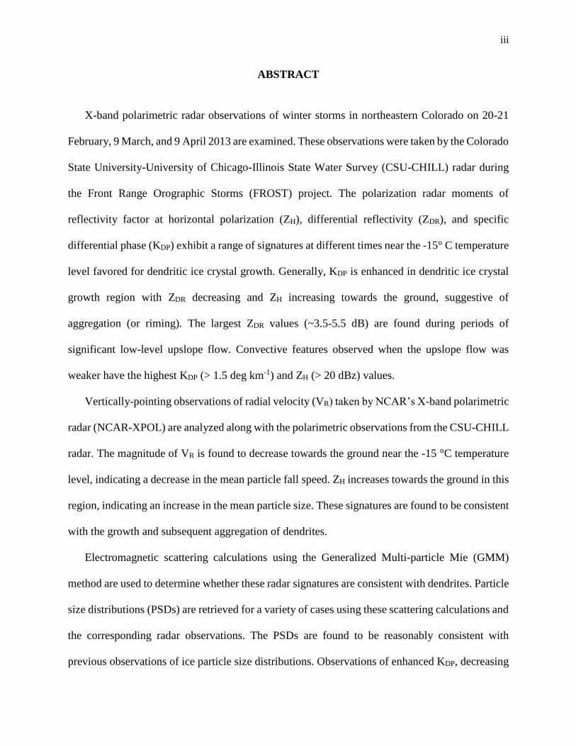
ABSTRACT
X-band polarimetric radar observations of winter storms in northeastern Colorado on 20-21
February, 9 March, and 9 April 2013 are examined. These observations were taken by the Colorado
State University-University of Chicago-Illinois State Water Survey (CSU-CHILL) radar during
the Front Range Orographic Storms (FROST) project. The polarization radar moments of
reflectivity factor at horizontal polarization (ZH), differential reflectivity (ZDR), and specific
differential phase (KDP) exhibit a range of signatures at different times near the -15° C temperature
level favored for dendritic ice crystal growth. Generally, KDP is enhanced in dendritic ice crystal
growth region with ZDR decreasing and ZH increasing towards the ground, suggestive of
aggregation (or riming). The largest ZDR values (~3.5-5.5 dB) are found during periods of
significant low-level upslope flow. Convective features observed when the upslope flow was
weaker have the highest KDP (> 1.5 deg km-1) and ZH (> 20 dBz) values.
Vertically-pointing observations of radial velocity (VR) taken by NCAR’s X-band polarimetric
radar (NCAR-XPOL) are analyzed along with the polarimetric observations from the CSU-CHILL
radar. The magnitude of VR is found to decrease towards the ground near the -15 °C temperature
level, indicating a decrease in the mean particle fall speed. ZH increases towards the ground in this
region, indicating an increase in the mean particle size. These signatures are found to be consistent
with the growth and subsequent aggregation of dendrites.
Electromagnetic scattering calculations using the Generalized Multi-particle Mie (GMM)
method are used to determine whether these radar signatures are consistent with dendrites. Particle
size distributions (PSDs) are retrieved for a variety of cases using these scattering calculations and
the corresponding radar observations. The PSDs are found to be reasonably consistent with
previous observations of ice particle size distributions. Observations of enhanced KDP, decreasing

iv
ZDR, and increasing ZH towards the ground may therefore be useful in identifying regions of rapidly
collecting dendrites and thus increased surface snowfall rates.

v
TABLE OF CONTENTS
List of Tables……………………………………………………………………………. vi
List of Figures…………………………………………………………………………... vii
Preface………………………………………………………………………………….. xii
Acknowledgements…………………………………………………………………..... xiii
Chapter 1. INTRODUCTION…………………………………………………………..... 1
1.1 Dendritic Ice Crystal Growth and Aggregation……………………………… 1
1.2 Polarimetric Weather Radar Background.………………………………….... 3
1.3 Previous Polarimetric Observations of Pristine Ice Crystals............................ 7
Chapter 2. DATA AND METHODS…………………………………………………… 10
Chapter 3. OVERVIEW OF WINTER STORM CASES………………………………. 13
Chapter 4. RADAR SIGNATURES OF DENDRITIC GROWTH…………………….. 23
Chapter 5. VERTICAL PROFILES OF RADAR OBSERVATIONS…………………. 33
5.1 Signatures of Riming, Dendritic Growth and Aggregation……..………….. 33
5.2 Radar Observations with Temperature………………………..……………. 36
Chapter 6. ELECTROMAGNETIC SCATTERING CALCULATIONS………….…... 44
6.1 Description and Monodisperse Distribution Calculations…………….…..... 44
6.2 Ice PSD retrieval with Mixtures of Aggregates…………………………...... 47
Chapter 7. DISCUSSION……………………………………………………………..... 61
Chapter 8. CONCLUSIONS…………………………………………………………..... 72
Appendix A: ALTERNATIVE KDP ESTIMATION PROCEDURE………………....... 75
References……………………………………………………………………………..... 78

vi
LIST OF TABLES
Table 6.1 Description of the plates and dendrites from the database shown in Botta (2013). Adapted
from Lu et al. (2014)…………………………………………………………………………...... 53
Table 6.2. Exponential ice PSDs determined from the radar observations listed in columns 2, 5 and
6. An aggregate ZDR of 0.3 dB and σ = 15° are assumed for these calculations………………… 53
Table 7.1. Percentage changes in N0 and λ with respect to the values shown in table 3, for 20%
perturbations in ZDR and KDP……………………………………………………………………. 67
Table 7.2. Percentage changes in N0 and λ with respect to the values shown in table 3, for aggregate
ZDR values of 0.0 and 0.6 dB…………………………………………………………………….. 68
Table 7.3. Percentage changes in N0 and λ with respect to the values shown in table 3, for crystal
types of p1.0 and d0.5. No modification of crystal type was imposed on the 9 April case…...… 68
Table 7.4. Gamma ice PSDs determined from the radar observations listed in columns 2, 5 and 6.
An aggregate ZDR of 0.3 dB and σ = 15° are assumed for these calculations…………………… 69
vii
LIST OF FIGURES
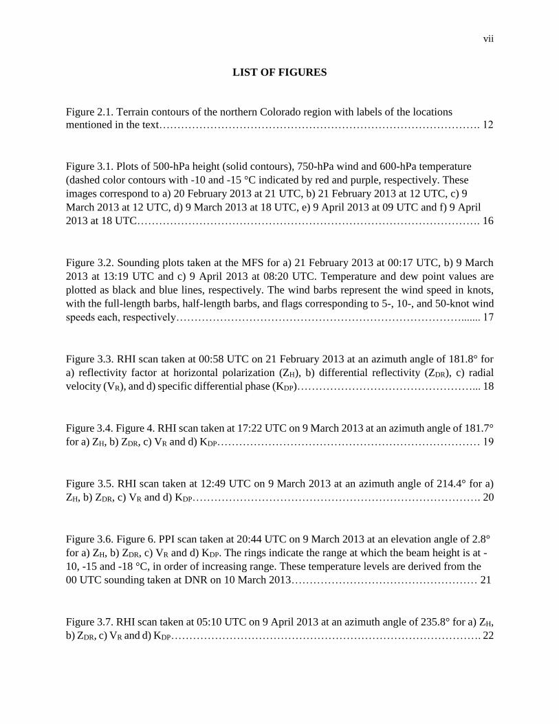
Figure 2.1. Terrain contours of the northern Colorado region with labels of the locations
mentioned in the text……………………………………………………………………………. 12
Figure 3.1. Plots of 500-hPa height (solid contours), 750-hPa wind and 600-hPa temperature
(dashed color contours with -10 and -15 °C indicated by red and purple, respectively. These
images correspond to a) 20 February 2013 at 21 UTC, b) 21 February 2013 at 12 UTC, c) 9
March 2013 at 12 UTC, d) 9 March 2013 at 18 UTC, e) 9 April 2013 at 09 UTC and f) 9 April
2013 at 18 UTC…………………………………………………………………………………. 16
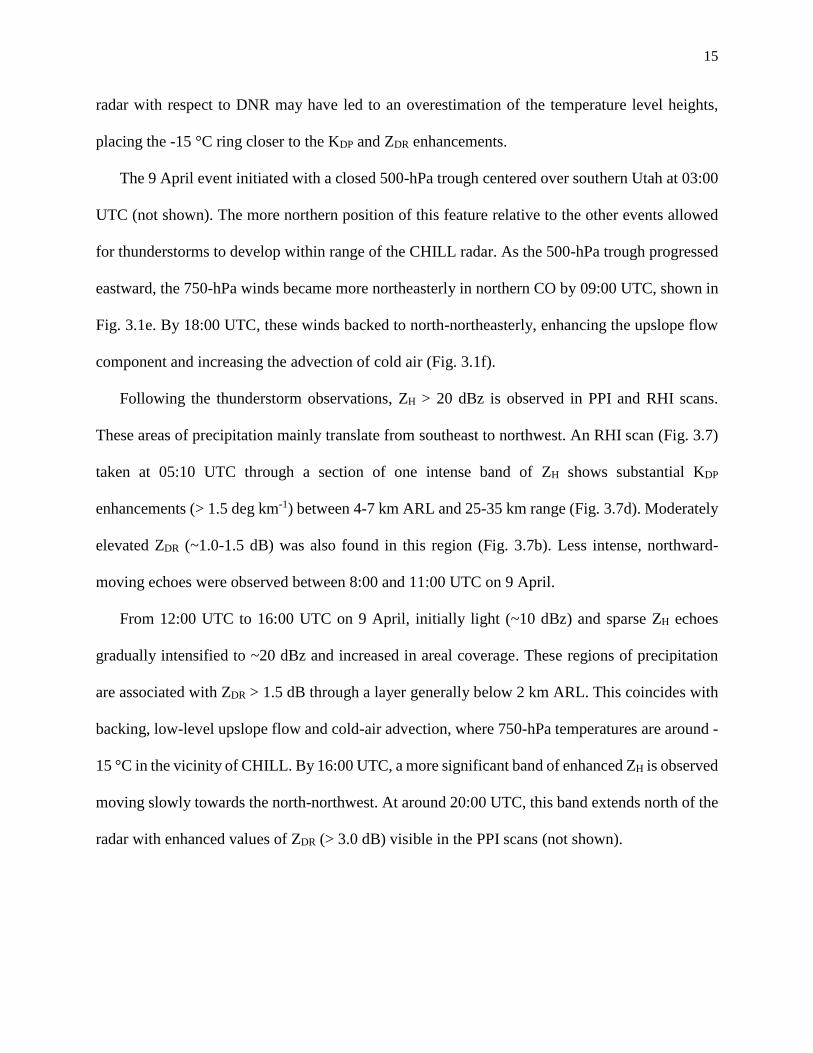
Figure 3.2. Sounding plots taken at the MFS for a) 21 February 2013 at 00:17 UTC, b) 9 March
2013 at 13:19 UTC and c) 9 April 2013 at 08:20 UTC. Temperature and dew point values are
plotted as black and blue lines, respectively. The wind barbs represent the wind speed in knots,
with the full-length barbs, half-length barbs, and flags corresponding to 5-, 10-, and 50-knot wind
speeds each, respectively……………………………………………………………………....... 17
Figure 3.3. RHI scan taken at 00:58 UTC on 21 February 2013 at an azimuth angle of 181.8° for
a) reflectivity factor at horizontal polarization (ZH), b) differential reflectivity (ZDR), c) radial
velocity (VR), and d) specific differential phase (KDP)…………………………………………... 18
Figure 3.4. Figure 4. RHI scan taken at 17:22 UTC on 9 March 2013 at an azimuth angle of 181.7°
for a) ZH, b) ZDR, c) VR and d) KDP……………………………………………………………… 19
Figure 3.5. RHI scan taken at 12:49 UTC on 9 March 2013 at an azimuth angle of 214.4° for a)
ZH, b) ZDR, c) VR and d) KDP……………………………………………………………………. 20
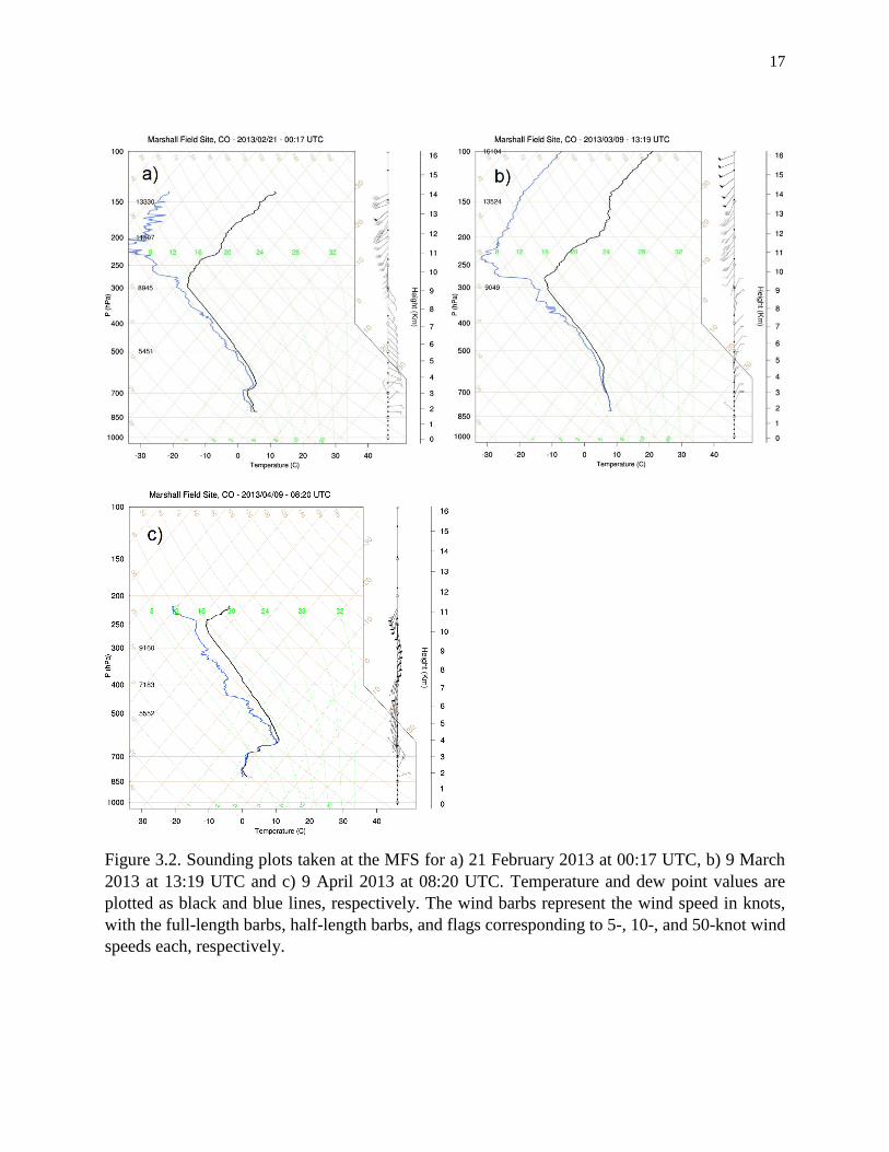
Figure 3.6. Figure 6. PPI scan taken at 20:44 UTC on 9 March 2013 at an elevation angle of 2.8°
for a) ZH, b) ZDR, c) VR and d) KDP. The rings indicate the range at which the beam height is at -
10, -15 and -18 °C, in order of increasing range. These temperature levels are derived from the
00 UTC sounding taken at DNR on 10 March 2013…………………………………………… 21
Figure 3.7. RHI scan taken at 05:10 UTC on 9 April 2013 at an azimuth angle of 235.8° for a) ZH,
b) ZDR, c) VR and d) KDP…………………………………………………………………………. 22
viii
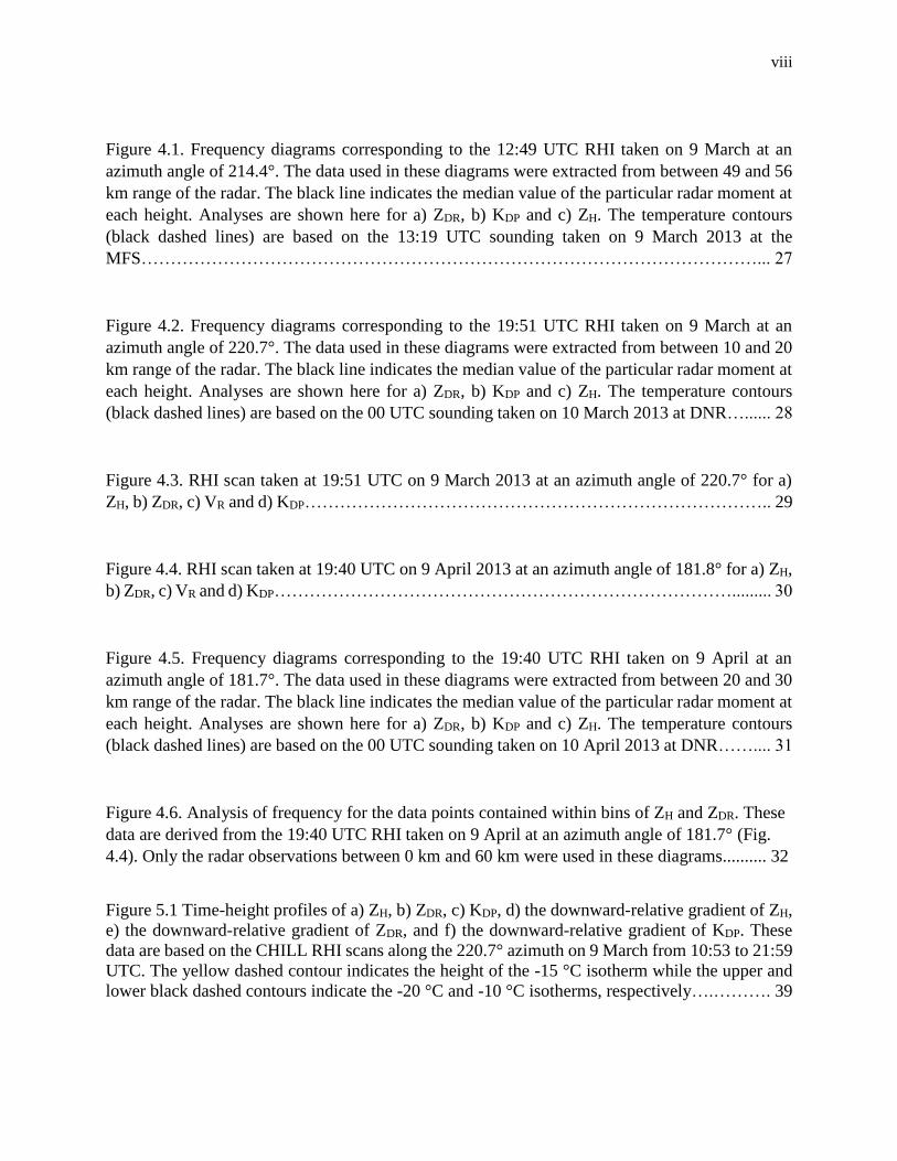
Figure 4.1. Frequency diagrams corresponding to the 12:49 UTC RHI taken on 9 March at an
azimuth angle of 214.4°. The data used in these diagrams were extracted from between 49 and 56
km range of the radar. The black line indicates the median value of the particular radar moment at
each height. Analyses are shown here for a) ZDR, b) KDP and c) ZH. The temperature contours
(black dashed lines) are based on the 13:19 UTC sounding taken on 9 March 2013 at the
MFS……………………………………………………………………………………………... 27
Figure 4.2. Frequency diagrams corresponding to the 19:51 UTC RHI taken on 9 March at an
azimuth angle of 220.7°. The data used in these diagrams were extracted from between 10 and 20
km range of the radar. The black line indicates the median value of the particular radar moment at
each height. Analyses are shown here for a) ZDR, b) KDP and c) ZH. The temperature contours
(black dashed lines) are based on the 00 UTC sounding taken on 10 March 2013 at DNR…...... 28
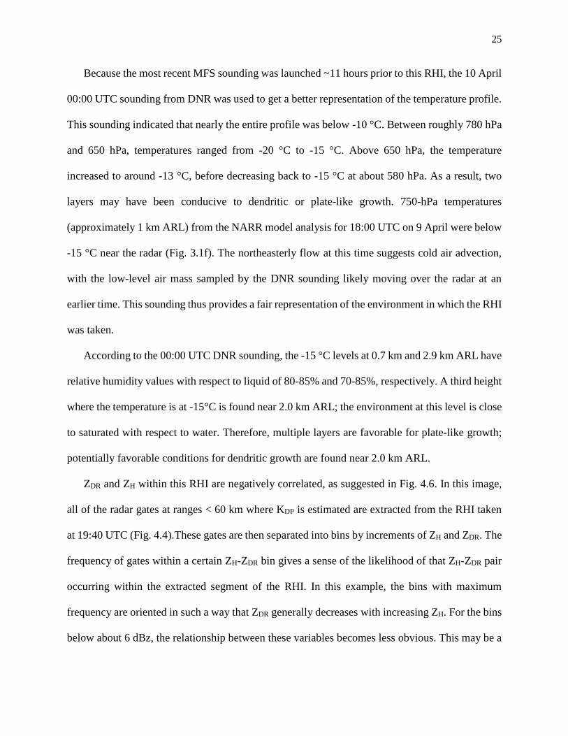
Figure 4.3. RHI scan taken at 19:51 UTC on 9 March 2013 at an azimuth angle of 220.7° for a)
ZH, b) ZDR, c) VR and d) KDP…………………………………………………………………….. 29
Figure 4.4. RHI scan taken at 19:40 UTC on 9 April 2013 at an azimuth angle of 181.8° for a) ZH,
b) ZDR, c) VR and d) KDP……………………………………………………………………......... 30
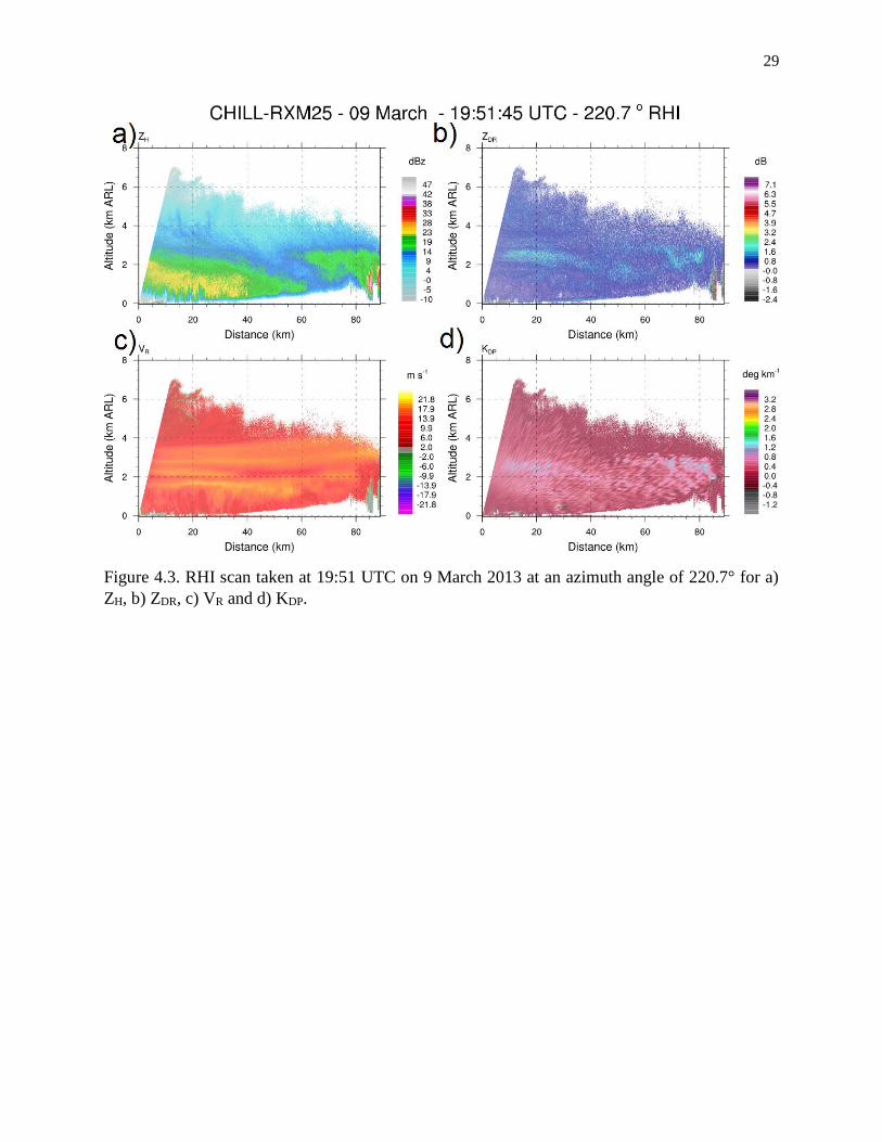
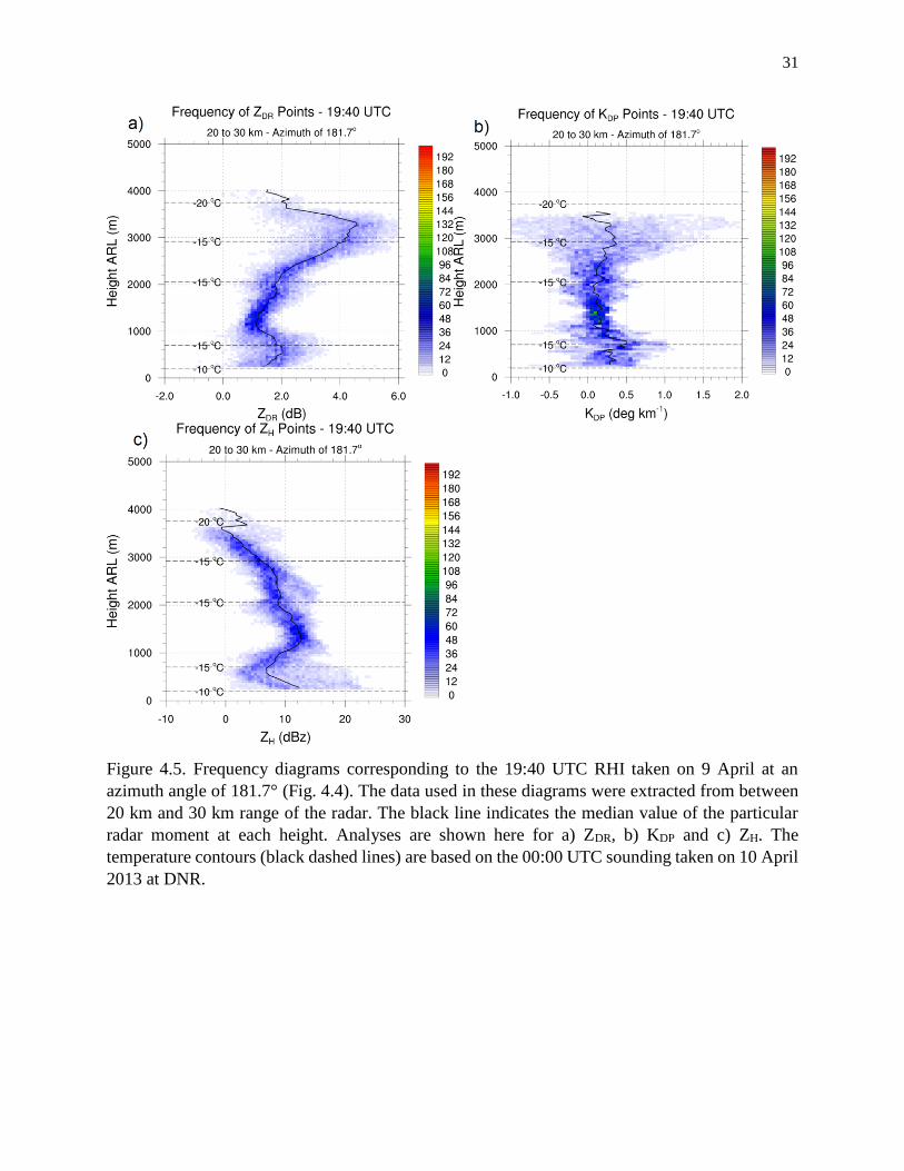
Figure 4.5. Frequency diagrams corresponding to the 19:40 UTC RHI taken on 9 April at an
azimuth angle of 181.7°. The data used in these diagrams were extracted from between 20 and 30
km range of the radar. The black line indicates the median value of the particular radar moment at
each height. Analyses are shown here for a) ZDR, b) KDP and c) ZH. The temperature contours
(black dashed lines) are based on the 00 UTC sounding taken on 10 April 2013 at DNR…….... 31
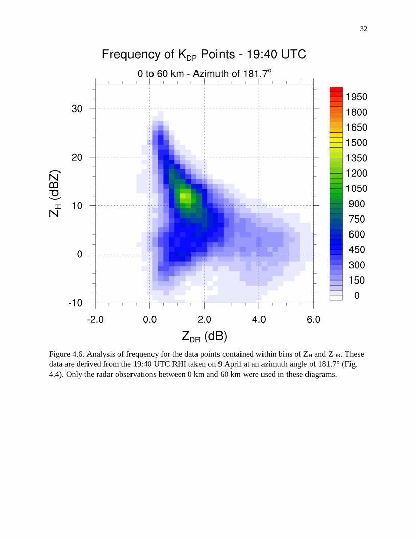
Figure 4.6. Analysis of frequency for the data points contained within bins of ZH and ZDR. These
data are derived from the 19:40 UTC RHI taken on 9 April at an azimuth angle of 181.7° (Fig.
4.4). Only the radar observations between 0 km and 60 km were used in these diagrams.......... 32
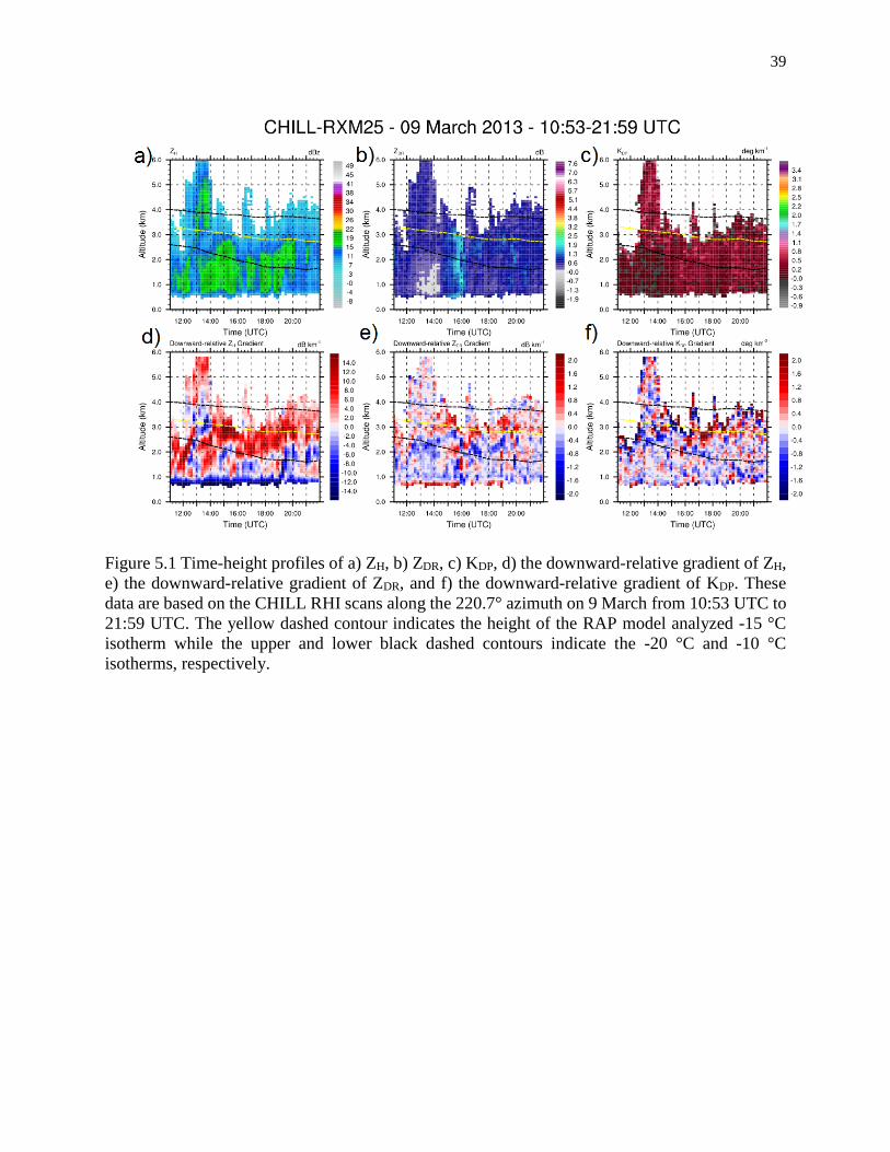
Figure 5.1 Time-height profiles of a) ZH, b) ZDR, c) KDP, d) the downward-relative gradient of ZH,
e) the downward-relative gradient of ZDR, and f) the downward-relative gradient of KDP. These
data are based on the CHILL RHI scans along the 220.7° azimuth on 9 March from 10:53 to 21:59
UTC. The yellow dashed contour indicates the height of the -15 °C isotherm while the upper and
lower black dashed contours indicate the -20 °C and -10 °C isotherms, respectively….………. 39

ix
Figure 5.2 Time-height profiles of a) ZH, b) VR, c) the downward-relative gradient of ZH, d) the
downward-relative gradient of VR. These data are based on the XPOL vertically-pointing scans
taken at the MFS on 9 March from 10:53 to 21:59 UTC. The yellow dashed contour indicates the
height of the -15 °C isotherm while the upper and lower black dashed contours indicate the -20 °C
and -10 °C isotherms, respectively…………………...…………………………………………. 40
Figure 5.3 Time-height profiles of a) ZH, b) ZDR, c) KDP, d) the downward-relative gradient of ZH,
e) the downward-relative gradient of ZDR, and f) the downward-relative gradient of KDP. These
data are based on the CHILL RHI scans along the 220.7° azimuth on 20-21 February from
approximately 22:40 to 02:40 UTC. The yellow dashed contour indicates the height of the -15 °C
isotherm while the upper and lower black dashed contours indicate the -20 °C and -10 °C
isotherms, respectively………………………………………………………...………………... 41
Figure 5.4 Time-height profiles of a) ZH, b) VR, c) the downward-relative gradient of ZH, d) the
downward-relative gradient of VR. These data are based on the XPOL vertically-pointing scans
taken at the MFS on 20-21 February from approximately 22:20 to 02:20 UTC. The yellow dashed
contour indicates the height of the -15 °C isotherm while the upper and lower black dashed
contours indicate the -20 °C and -10 °C isotherms, respectively………………………………... 42
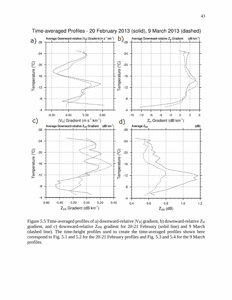
Figure 5.5 Time-averaged profiles of a) downward-relative |VR| gradient, b) downward-relative ZH
gradient, and c) downward-relative ZDR gradient for 20-21 February (solid line) and 9 March
(dashed line). The time-height profiles use to create the time-averaged profiles shown here
correspond to figures 5.1 and 5.2 for the 20-21 February profiles and figures 5.3 and 5.4 for the 9
March profiles…………………………………………………………………………………... 43
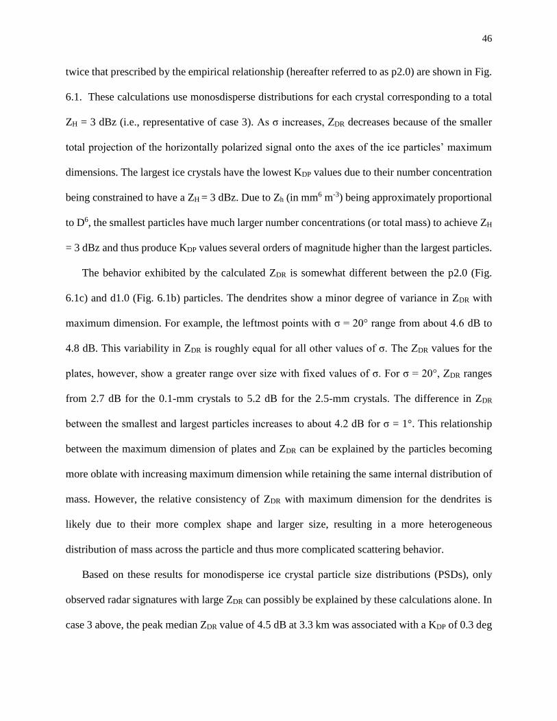
Figure 6.1. Scattering calculations for monodisperse populations of a) dendrites with one half the
reference thickness, b) dendrites of the reference thickness and c) plates twice the reference
thickness based on the empirical relationships found in Auer and Veal (1970). The ZH values for
all data points are 3 dBz. The numbers labeled to the right of the data indicate the maximum
dimension (in mm) and number concentration (in m-3) for the size class of ice particles,
respectively. The color of the points differentiate the crystals sizes for which the scattering
calculations are performed. The size of the markers indicates the canting angle distribution width
(σ) with the largest markers equal to 20° and the smallest markers equal to 1°………………… 54
Figure 6.2. Plot of ZHI given observations of ZH
T and ZDRT, a value of ZDR
I of 5.8 dB and a ZDRA
value of 0.3 dB………………………………………………………………………………....... 55
Figure 6.3. Schematic depicting the iterative process by which a PSD is retrieved from a set of
radar observations. The orange-colored boxes indicate the quantity is observed by the radar, the

x
blue-colored boxes indicate the quantity is derived from the radar observations and scattering
calculations and the green-colored box indicates an assumed quantity…………………………. 56
Figure 6.4. Contours of KDPI (blue) and the ZH
I contribution from ice (red) as a function of the
slope and intercept parameters for PSDs of exponential form. ZHI is contoured every 2 dBz from
0 to 20 dBz………………………………………………………………………………………. 57
Figure 6.5. Plot of the number concentration per size (maroon), marginal contribution to Zh
(orange) and marginal contribution to KDP (blue) corresponding to the exponential PSD with N0 =
1.84x10⁵ m3 mm-1 and λ= 3.29 mm-1. Ice particles to the left of the red dashed line are of type p1.0
and of type d1.0 to the right…………………………………………………………………........ 58
Figure 6.6. Plot of the number concentration per size (maroon), marginal contribution to Zh
(orange) and marginal contribution to KDP (blue) corresponding to the exponential PSD with N0 =
5.91x10⁴ m3 mm-1 and λ= 1.87 mm-1. Ice particles to the left of the red dashed line are of type p1.0
and of type d1.0 to the right…………………………………………………………………….... 59
Figure 6.7. Plot of the number concentration per size (maroon), marginal contribution to Zh
(orange) and marginal contribution to KDP (blue) corresponding to the exponential PSD with N0 =
3.85x10⁵ m3 mm-1 and λ= 7.13 mm-1. The ice particles used here are all of type p2.0………….. 60
Figure 7.1. Number concentration per unit size as a function of maximum dimension based several
observational probe studies. The orange curve corresponds to the ice particle observations taken
at temperatures between -10 and -20 °C. From Heymsfield et al. (2013). The dots depict the values
one standard deviation above the mean normalized concentrations at each temperature range and
diameter…………………………………………………………………………………………. 70
Figure 7.2. Plots of the number concentration per size (maroon), marginal contribution to Zh
(orange) and marginal contribution to KDP (blue) for a) particles of type p2.0 and d1.0 and b) type
p2.0 and d0.5. The maroon dashed lines shows the bulk PSD observations adapted from the
Heymsfield et al. (2013) study (Fig. 7.1)…………………………………………………........... 71
Figure A1. Frequency distributions with height of KDP calculated using the a) WC09 estimation
procedure and b) the alternate estimation procedure described in appendix A (identical to Fig.
4.5b). These distributions correspond to the RHI taken at 19:40 UTC on 9 April at an azimuth
angle of 181.7°. These data have been extracted at ranges between 20 and 30 km. The black dashed

xi
lines indicate the temperature levels derived from the 00 UTC sounding from DNR on 10
April…………………………………………………………………………………………….. 77

xii
PREFACE
This thesis contains significant elements from an article of which I am first author, and has
been preliminarily accepted pending major revisions in the Journal of Applied Meteorology and
Climatology. Matt Kumjian and Yinghui Lu are the two listed co-authors of this paper. I
contributed the majority of the elements contained in the Abstract, Chapters 1-5, Chapters 7-8 and
Appendix A. Yinghui Lu provided the scattering calculations appearing in Chapter 6.
xiii
ACKNOWLEDGEMENTS
I would like to thank Patrick C. Kennedy, Steve Rutledge, and Francesc Junyent (CSU) for
help coordinating, collecting, and processing the CSU-CHILL data used in this study. I thank my
advisor Matt Kumjian, thesis committee members Hans Verlinde and Eugene Clothiaux, and
Kultegin Aydin and Jerry Harrington for their insights regarding this work.
I thank Matt Kumjian and Yinghui Lu for their work as co-authors on the paper mentioned
in the preface. Funding for this work (Robert S. Schrom and Matt Kumjian) comes from NSF grant
AGS-1143948. Yinghui Lu is funded through NSF grant AGS-1228180. I acknowledge the
American Meteorological Society as the sole copyright holder of the article comprising a portion
of this thesis.

1
CHAPTER 1. INTRODUCTION
Winter storms often have severe impacts on society, both economically and through increased
risks to life and property. However, accurate short-term forecasting of these events remains a
challenge. One of the greatest areas of uncertainty in these forecasts comes from a poor
understanding of the microphysical processes that contribute to the development of heavy snow.
Part of this lack of understanding is a result of the limited observations of ice particles within
winter storms. Several recent studies have attempted to overcome the limited in situ measurements
by examining the polarimetric radar signatures found in the dendritic growth zones of these storms
(e.g. Kennedy and Rutledge 2011; Andrić et al. 2013; Bechini et al. 2013). However, these studies
are themselves limited due to the narrow range of cases explored and a lack of correspondence
between the radar observations and scattering model simulations. Therefore, the need to explore
the variability of the radar signatures and the scattering of ice particles within dendritic growth
zones motivates this study.
1.1 Dendritic Ice Crystal Growth and Aggregation
The processes by which ice particles increase mass are vapor depositional growth, collection
of ice particles, and collection of supercooled water. Snow growth through aggregation is enhanced
when dendritic ice crystals are present. Dendrites are favored to grow in temperatures near -15 °C
and ice supersaturations above 0.15 (e.g., Bailey and Hallett 2009). Aggregates that form rapidly
through the collection of dendrites can increase the snowfall accumulation rate (Lamb and
Verlinde 2011) and decrease visibility near the ground (Rasmussen et al. 1999). Thus, from an
operational perspective, vapor depositional growth of dendrites and aggregation are important
2
microphysical processes to identify observationally, improving near-term forecasts of winter
storms.
The growth of ice crystals by vapor deposition is important in the initial development of the
ice particle population within a cloud. These crystals first appear as ice nuclei that accumulate
vapor mass in an environment supersaturated with respect to ice (Pruppacher and Klett 1997, pg.
547). Depending on the temperature of the environment, water vapor will attach to the ice lattice
of a particle preferentially along either the basal or prism faces of the crystal (Lamb and Scott
1972). Dimensions along the basal and prism faces of a hexagonal ice crystal can be defined using
two orthogonal axes: the c-axis, normal to the two hexagonal basal faces, and the a-axis, normal
to one of the six rectangular prism faces. The aspect ratio of an ice crystal can thus be defined as
the ratio of the c- and a-axes; aspect ratios are less than one for plate-like ice crystals. When
temperatures are around -15 °C, the prism faces experience the quickest growth, leading to the
formation of oblate crystals (Chen and Lamb 1994). If these particles continue to grow in
temperatures where the prism faces grow fastest, the gradient in water vapor along these faces
increases with decreasing aspect ratio (Marshall and Langleben 1954). This increased vapor
gradient increases the growth rate of the particle along the prism faces, further decreasing the
aspect ratio.
Once ice crystals are sufficiently large, they begin to collect each other. This mass growth by
collection of ice particles is known as aggregation. One factor determining the aggregation rate is
the relative fall speeds of the faster-falling particles with respect to slower-falling ice crystals to
be collected. The larger their differences in fall speed, the larger the effective volumes that are
swept out by the collecting particles over a given time. These effective volumes also depend on
the cross-sectional areas of the particles.

3
Fall speeds of ice are dependent on crystal habit. Laboratory and theoretical studies (e.g.,
Harrington et al. 2013) show a minimum in fall speed for ice crystals growing in temperatures near
-15 °C. These slower fall speeds result from the large cross-sectional area to mass ratio of the low
aspect ratio crystals that form under these conditions. Therefore, collection of these dendritic ice
crystals by snow aggregates will be enhanced due to the increased differential in fall speeds
between the dendrites and snow aggregates.
Another important factor influencing the rate of aggregation is the collection efficiency. This
collection efficiency depends on the properties of both particles interacting during a discrete
collection event. The branched structure found in dendrites enhances the collection efficiency due
to the increased effective roughness of the particles. Connelly et al. (2012) found a maximum in
the collection efficiency at -15 °C by comparing laboratory-grown ice crystals with model
simulations.
1.2 Polarimetric Weather Radar Background
Dual-polarization radar provides information related to the orientation, shape, and diversity of
the sampled hydrometeors. The National Weather Service array of WSR-88D radars has recently
been upgraded to dual-polarization, allowing for this valuable information to be used operationally
(e.g., Doviak and Zrnić 1993; Zrnić and Ryzhkov 1999; Bringi and Chandrasekar 2001; Ryzhkov
et al. 2005a; Kumjian 2013a,b,c and references therein). Thus, information about the microphysics
of precipitation provided by these instruments can be used by weather forecasters operationally.
The scattering properties of hydrometeors allow for the orientation, shape, and diversity
information of the particles to be retrieved from polarimetric radar. As an electromagnetic wave
4
interacts with a particle, radiation will be scattered in a way that depends on the incident electric
field and the properties of the particle. These properties include the size of the particle relative to
the wavelength of the radiation (electromagnetic size), and the particle’s density, phase
composition, shape, and orientation. For un-melted ice particles, the effective density of the
particle determines the particle’s effective dielectric constant, ε at a particular wavelength. This
effective dielectric constant is typically modeled as a mixture of ice and air (e.g. Maxwell Garnett
1904), with low density particles having a real part of ε that is small. Therefore, solid ice particles,
such as plate crystals, will have greater values of ε than low-density snow aggregates.
The information of most interest in radar applications is the electromagnetic radiation
backscattered to the antenna at an angle 180° from the propagation direction of the transmitted
radar beam. This backscattered radiation can be expressed as (Bringi and Chandrasekar 2001):
[𝐸ℎ
𝑠
𝐸𝑣𝑠] =
𝑒−𝑗𝑘0𝑟
𝑟[𝑆ℎℎ
𝜋 𝑆𝒉𝒗𝝅
𝑆𝒗𝒉𝝅 𝑆𝒗𝒗
𝝅] [𝐸ℎ
𝑖
𝐸𝑣𝑖], (1.1)
where Sklπ
are the elements of the backscattering amplitude matrix (S) at the incident polarization,
“l”, and scattered polarization, “k”, r is the distance from the radar, and Eh,vs,i is the electric field
component with the subscript denoting the polarization and with the superscript “s” denoting
scattered and “i” denoting incident. Equation (1.1) shows that S transforms the incident
electromagnetic wave to the backscattered electromagnetic wave. S can be estimated using
numerical techniques such as the T-matrix (e.g., Waterman 1971; Mishchenko 2000) or the
Generalized Multi-particle Mie (GMM; Xu 1995, Xu and Gustafson 2001) method.
To better understand the effects of the aspect ratio on the scattering properties of ice
particles, the Rayleigh approximation is used. In this approximation, the incident electric field is
5
assumed to be constant over the particle, with the scattered electric field represented by a dipole
dependent on the particle’s polarizability (van de Hulst 1981). The polarizability can be found
analytically if the particle is modeled as a spheroid. For horizontally oriented spheroids, the cross-
polar elements (Shv and Svh) of the amplitude scattering matrix are equal to zero, further simplifying
the problem. Radar reflectivity factor at horizontal and vertical polarization (Zh,v) for a single
particle is defined as (Doviak and Zrnić 1993):
𝑍ℎ,𝑣 =4𝜆4
𝜋4|𝐾𝑤|2 |𝑆ℎℎ,𝑣𝑣𝜋|
2, (1.2)
where λ is the wavelength and Kw is the dielectric factor of liquid water. In the Rayleigh
approximation, Zh,v is proportional to the equivalent volume diameter of the particle to the sixth
power. The differential reflectivity (Zdr) is related to the ratio of the co-polar elements of S by
(Doviak and Zrnić 1993)
𝑍𝑑𝑟 =|𝑆ℎℎ
𝜋|2
|𝑆𝑣𝑣𝜋|2 . (1.3)
Oblate spheroids will have larger |𝑆ℎℎ| components than |𝑆𝑣𝑣| components and thus positive ZDR,
where ZDR = 10log10(Zdr). ZDR will therefore increase with decreasing aspect ratio.
To retrieve the bulk polarimetric moments defined in (1.2) and (1.3) for a population of
particles, each equation must be integrated over a distribution of sizes and orientations.
Hydrometeors, however, modulate the electromagnetic wave as it propagates from the radar to a
particular sampling volume and back. Both the phase and amplitude of the electromagnetic wave
change as it propagates through the distributed medium of hydrometeors. Given the presence of

6
non-spherical hydrometeors, there will be a differential phase shift between the horizontally and
vertically polarized wave components. This differential phase shift (ΦDP) will accumulate through
the entire propagation path of the transmitted signal. To better represent the contribution to ΦDP
from hydrometeors at a particular range, specific differential phase (KDP) is defined as one-half
the range derivative of ΦDP. Propagation effects are defined using the forward scattering
amplitudes of the particles. In the Rayleigh approximation, the forward scattering amplitudes,
𝑆ℎℎ,𝑣𝑣0, are equivalent to 𝑆ℎℎ,𝑣𝑣
𝜋 (Van de Hulst 1981). KDP for a single particle is defined as
(Bringi and Chandrasekar 2001)
𝐾𝐷𝑃 = 180𝜆
𝜋𝑅𝑒[𝑆ℎℎ
𝜋 − 𝑆𝑣𝑣𝜋]. (1.4)
As shown by equation (1.4), oblate spheroids satisfying the Rayleigh approximation will therefore
have positive values of KDP.
For a size distribution N(D) of horizontally-oriented spheroids, equations (1.2), (1.3) and
(1.4) can be written (dropping the “π” superscript) as
𝑍ℎ,𝑣 = 4𝜆4
𝜋4|𝐾𝑤|2 ∫ |𝑆ℎℎ,𝑣𝑣(𝐷)|2
𝑁(𝐷)𝑑𝐷∞
0, (1.5)
𝑍𝑑𝑟 = 𝑍ℎ
𝑍𝑣, (1.6)
𝐾𝐷𝑃 = 180𝜆
𝜋∫ 𝑅𝑒[𝑆ℎℎ(𝐷) − 𝑆𝑣𝑣(𝐷)]
∞
0𝑁(𝐷)𝑑𝐷. (1.7)
From equations (1.5) and (1.6), it can be seen that Zdr will be independent of the number
concentration of hydrometeors present in a sampling volume. However, Zdr will be weighted
7
strongly by the largest particles due to Zh,v being proportional to D6. In contrast, KDP is mass-
weighted because Re(Shh) is proportional to D3, and is dependent on the number concentration of
anisotropic scatterers. For hydrometeors with an orientation distribution, the polarimetric moments
can be determined using angular moments (e.g., Ryzhkov et al. 2011). This limited theoretical
background provides a basis to interpret the radar observations of winter storms at X band.
1.3 Previous Studies Using Polarimetric Observations of Pristine Ice Crystals
Enhancements in KDP and ZDR above the melting layer have been observed by a number of
studies (e.g. Ryzhkov and Zrnić 1998; Trapp et al. 2001; Wolde and Vali 2001; Kennedy and
Rutledge 2011; Andrić et al. 2013; Bechini et al. 2013; Schneebeli et al. 2013; Kumjian et al. 2014;
Griffin et al. 2014). This signature has been linked to the presence of dendrites and plate-like ice
crystals.
Kennedy and Rutledge (2011) found ZDR and KDP maxima with S-band radar near the -15° C
level for several winter storm cases. The presence of these enhancements was correlated with
increased snowfall rates at the ground. They compared these radar observables and ZH (where ZH
= 10log10[Zh]) with electromagnetic scattering calculations using the T-matrix method for
distributions of ice particles. The distributions used in their study were based on airplane ice
particle size distribution (PSD) observations (Lo and Passarelli 1982). Observed KDP and ZH values
were reproduced with these PSDs; however, the resulting ZDR signature was greater than that found
in the observations.
Andrić et al. (2013) found similar ZDR and KDP signatures in S-band radar observations of
winter storms. They also performed scattering calculations with PSDs of plates, dendrites, and
8
aggregates determined from the results of a one-dimensional microphysical model. The scattering
calculations in this study were based on the Rayleigh approximation. As in Kennedy and Rutledge
(2011), the calculated radar variables failed to reproduce all of the observed polarimetric
signatures. Large concentrations of ice crystals produced through secondary ice generation, not
present in their model, were proposed to explain the discrepancy between the calculated and
observed KDP.
Bechini et al. (2013) also observed enhancements in ZDR and KDP with X- and C-band radars
around the -15 °C level within stratiform precipitation. This signature was attributed to the
presence of dendritic crystals. The observed KDP was found to scale inversely with wavelength and
ZH was found to be independent of wavelength, suggesting these particles were
electromagnetically small. The scattering calculations used to verify this were based on those
performed by Kennedy and Rutledge (2011), with T-matrix calculations for the spheroidal
particles performed at both X and C band. No discussion of the correspondence between the
scattering calculations and the radar observations was provided.
The lack of agreement in these studies between electromagnetic scattering calculations and
radar observations necessitates both a better understanding of the variability of the radar signatures
in regions of possible dendritic growth and a better representation of the scattering of ice crystals,
where the distribution of mass deviates significantly from uniform spheroidal particles. This study
uses X-band polarimetric radar data from several winter storms in Colorado to examine a range of
signatures in regions of dendritic crystal growth. Advanced scattering calculations are also used to
determine PSDs that match each of the observed radar signatures. The physical validity of the
resulting PSDs is assessed by comparison with previous observational studies of ice crystal PSDs.

9
A description of the data used in this study is introduced in the next chapter. An overview of
the meteorological background for the events of study is presented in chapter 3. Chapter 4 provides
a detailed analysis of the radar signatures found within the events and statistics characterizing these
signatures. Chapter 5 is an analysis of the vertically-pointing radar observations and the
polarimetric radar observations at the same location. A description and analysis of the scattering
calculations used in this study are found in chapter 6. Chapter 7 contains a discussion of the
sensitivity and physical implications of the resulting PSDs. The main conclusions of this study are
provided in chapter 8.

10
CHAPTER 2. DATA AND METHODS
For this study, data from the Front Range Orographic Storms project (FROST; Kumjian et al.
2014) in northeastern Colorado are used. Significant winter storm events on 20-21 February, 9
March, and 9 April 2013 are the focus of this paper. Data collected during these events include
radar observations from the CSU-CHILL radar (Brunkow et al. 2000) and soundings launched at
the Marshall Field Site (MFS); these locations are shown in Fig. 2.1. The CHILL radar and MFS
are at elevations of 1432 m and 1742 m MSL, respectively.
The CHILL radar has recently been upgraded to a dual-wavelength system with X- and S-band
frequencies (Junyent et al. 2014). In FROST, the X-band frequency was used due to its smaller
beam width (0.3°) and greater sensitivity to KDP. CHILL data are available between 19:00 UTC
on 20 February to 12:00 UTC on 21 February, 10:29 UTC to 22:02 UTC on 9 March, and 00:41
UTC to 22:33 UTC on 9 April. The radar data contain a series of PPI and RHI scans performed
every ~12 minutes. The PPI and RHI scans were mostly performed at a set of fixed elevation and
azimuth angles, respectively. The azimuth angles of the RHI scans occasionally varied depending
on the appearance of precipitation targets. A full description of this field project can be found in
Kumjian et al. (2014).
During the events on 20-21 February and 9 March, NCAR’s mobile X-band polarimetric radar
(NCAR-XPOL) was scanning concurrently with the CHILL. This radar was located at the MFS
during these events and provided vertically pointing observations, as well as RHI and PPI scans,
of ZH and radial velocity (VR), along with the polarimetric moments. However, at vertical
incidence, most of the shape information content contained in the polarimetric moments is lost.
Vertical scans taken by the XPOL are available from 22:16 UTC to 02:21 UTC on 20-21
February and from 02:59 UTC to 23:51 UTC on 9 March. These data are compiled into time-

11
height cross-sections by averaging ZH and VR over the ~3 minute scans. The period between
consecutive scans is every ~12 minutes, with each time-averaged profile representing one of these
intervals.
To compare the XPOL observations with the polarimetric moments observed by the CHILL
at roughly horizontal incidence, vertical profiles over the XPOL are constructed from CHILL
RHIs. RHIs taken along the 220.7° azimuth of the CHILL passed over the MFS at a range of 73
km and thus are used to create the vertical profiles. These profiles are produced by binning the
RHI gates into 75-m height increments: the same value as the gate width of the XPOL and slightly
greater than the ~51 m beam width of the CHILL at this range. For each height bin, the median
values of all ZH, ZDR, and KDP observations within 1 km of the MFS are taken to represent the
polarimetric moments at that height. Temperature level information comes from the Rapid Refresh
(RAP; Brown et al. 2011) model hourly analyses for each date and time range.
For the processed CSU-CHILL data, KDP is calculated from ΦDP using the Wang and
Chandrasekar (2009; herein WC09) method, which uses an adaptive algorithm to smooth ΦDP to a
degree inversely related to the signal to noise ratio. Before any range derivatives are computed in
the WC09 method, the data are first flagged in regions of high noise using the dispersion of ΦDP
over a number of consecutive gates. These flagged regions are set to KDP = 0 deg km-1, which may
introduce a large number of erroneous zero values that can skew statistical analyses and
microphysical interpretations. In order to eliminate these points, an alternative method of
estimating KDP (described in Appendix A) is used in this study. KDP observations produced with
this new scheme will be presented in later chapters.

12
Figure 2.2. Terrain contours of the northern Colorado region with labels of the locations
mentioned in the text.
13
CHAPTER 3. OVERVIEW OF WINTER STORM CASES
The events included in this study each featured similar synoptic evolutions. Information about
the synoptic-scale meteorological features present during these events is taken from the North
American Regional Reanalysis (NARR; Mesinger et al. 2006). One feature common to all events
is a 500-hPa trough progressing eastward through the central Rocky Mountains (Fig. 3.1). The
motion and position of the trough and its associated surface features helped dictate whether low-
level upslope flow was present in northeast Colorado.
The 20-21 February 2013 event was associated with a broad trough over the Rocky Mountains.
A closed low was present at 500 hPa in southwestern Arizona at 21:00 UTC on 20 February (Fig.
3.1a). At this time the 750-hPa (roughly 1 km above radar level, hereafter ARL) winds were mainly
easterly to southerly in northeastern Colorado. By 12:00 UTC on 21 February, the 500-hPa trough
axis was centered over central New Mexico and the low-level flow had become more northerly
(Fig. 3.1b). Cold-air advection was ongoing throughout the duration of the sampling period. The
height of the -15 °C level decreased from 2.8 km to 2.5 km ARL between 00:00 and 12:00 UTC
on 21 February, based on the radiosondes from Denver, CO (DNR). The sounding taken at the
Marshall Field Site at 00:17 UTC determined the height of the -15 °C level to be at about 2.6 km
ARL (Fig. 3.2a).
One of the notable features visible during this event is a narrow band of enhanced ZH (> 25
dBz) that approached the radar from the southeast between around 23:00 UTC on 20 February and
02:00 UTC on 21 February. An RHI scan taken at 00:58 UTC cutting through the axis of this band
shows enhancements in both ZDR and KDP (> 2.0 dB and 1.5 deg km-1, respectively) between 2.5-
4.0 km ARL and between 28-35 km range (Fig. 3.3). Temperatures within this height range were

14
between approximately -10 °C and -25 °C. After this period, lighter, generally less-organized
echoes are observed as weak upslope flow became the primary contributor to ascent.
At 12:00 UTC on 9 March, which was shortly after the onset of data collection, a closed 500-
hPa low was centered over the four corners region (Fig. 3.1c). There was generally northeasterly
flow at 750 hPa in northeastern CO at this time. By 18:00 UTC, the closed 500-hPa low was
positioned over southern CO, resulting in a stronger northerly component to the 750-hPa wind
within range of the CHILL radar (Fig. 3.1d). This can be seen in the RHI image from CHILL taken
at 17:22 UTC (Fig. 3.4). Between 1.0 km and 1.8 km ARL, the radial velocity is generally > 20 m
s-1, while above this level it is primarily < 10 m s-1 (Fig. 3.4c). This large gradient in radial velocity
is a consequence of the vertical shear between the low-level upslope regime and the mid-level flow
dictated by the synoptic-scale trough. This general flow regime continued through the termination
of data collection.
During the 9 March event, cold-air advection was occurring in northeastern CO. Mandated
soundings taken at DNR indicate the height of the -15 °C level decreased from 3.1 km to 2.6 km
ARL between 12:00 UTC 9 March and 00:00 UTC 10 March. The sounding taken at the MFS at
13:19 UTC (Fig. 3.2b) determined the -15 °C level to be around 3 km ARL.
Between 11:00 UTC and 14:00 UTC on 9 March, relatively more convective structures are
visible in PPI and RHI scans. An example of a significant convective feature found in an RHI
taken at 12:49 UTC is shown in Fig. 3.5. This time period is coincident with weaker, northeasterly
750-hPa flow. As these winds become stronger and more north-northeasterly, PPI scans show a
more stratiform distribution of precipitation. Figure 3.6 shows such a PPI image taken at an
elevation angle of 2.8° at 20:44 UTC on 9 March. Enhancements in ZDR and KDP are visible
between the range rings corresponding to -10 °C and -15 °C. The more northerly location of the
15
radar with respect to DNR may have led to an overestimation of the temperature level heights,
placing the -15 °C ring closer to the KDP and ZDR enhancements.
The 9 April event initiated with a closed 500-hPa trough centered over southern Utah at 03:00
UTC (not shown). The more northern position of this feature relative to the other events allowed
for thunderstorms to develop within range of the CHILL radar. As the 500-hPa trough progressed
eastward, the 750-hPa winds became more northeasterly in northern CO by 09:00 UTC, shown in
Fig. 3.1e. By 18:00 UTC, these winds backed to north-northeasterly, enhancing the upslope flow
component and increasing the advection of cold air (Fig. 3.1f).
Following the thunderstorm observations, ZH > 20 dBz is observed in PPI and RHI scans.
These areas of precipitation mainly translate from southeast to northwest. An RHI scan (Fig. 3.7)
taken at 05:10 UTC through a section of one intense band of ZH shows substantial KDP
enhancements (> 1.5 deg km-1) between 4-7 km ARL and 25-35 km range (Fig. 3.7d). Moderately
elevated ZDR (~1.0-1.5 dB) was also found in this region (Fig. 3.7b). Less intense, northward-
moving echoes were observed between 8:00 and 11:00 UTC on 9 April.
From 12:00 UTC to 16:00 UTC on 9 April, initially light (~10 dBz) and sparse ZH echoes
gradually intensified to ~20 dBz and increased in areal coverage. These regions of precipitation
are associated with ZDR > 1.5 dB through a layer generally below 2 km ARL. This coincides with
backing, low-level upslope flow and cold-air advection, where 750-hPa temperatures are around -
15 °C in the vicinity of CHILL. By 16:00 UTC, a more significant band of enhanced ZH is observed
moving slowly towards the north-northwest. At around 20:00 UTC, this band extends north of the
radar with enhanced values of ZDR (> 3.0 dB) visible in the PPI scans (not shown).

16
Figure 3.1. Plots of 500-hPa height (solid contours), 750-hPa wind and 600-hPa temperature
(dashed color contours with -10 °C and -15 °C indicated by red and purple, respectively. These
images correspond to a) 20 February 2013 at 21:00 UTC, b) 21 February 2013 at 12:00 UTC, c) 9
March 2013 at 12:00 UTC, d) 9 March 2013 at 18:00 UTC, e) 9 April 2013 at 09:00 UTC and f)
9 April 2013 at 18:00 UTC.
17
Figure 3.2. Sounding plots taken at the MFS for a) 21 February 2013 at 00:17 UTC, b) 9 March
2013 at 13:19 UTC and c) 9 April 2013 at 08:20 UTC. Temperature and dew point values are
plotted as black and blue lines, respectively. The wind barbs represent the wind speed in knots,
with the full-length barbs, half-length barbs, and flags corresponding to 5-, 10-, and 50-knot wind
speeds each, respectively.

18
Figure 3.3. RHI scan taken at 00:58 UTC on 21 February 2013 at an azimuth angle of 181.8° for
a) reflectivity factor at horizontal polarization (ZH), b) differential reflectivity (ZDR), c) radial
velocity (VR), and d) specific differential phase (KDP).

19
Figure 3.4. RHI scan taken at 17:22 UTC on 9 March 2013 at an azimuth angle of 181.7° for a)
ZH, b) ZDR, c) VR and d) KDP.

20
Figure 3.5. RHI scan taken at 12:49 UTC on 9 March 2013 at an azimuth angle of 214.4° for a)
ZH, b) ZDR, c) VR and d) KDP.
21
Figure 3.6. PPI scan taken at 20:44 UTC on 9 March 2013 at an elevation angle of 2.8° for a) ZH,
b) ZDR, c) VR and d) KDP. The rings indicate the range at which the beam height is at -10 °C, -15
°C and -18 °C, in order of increasing range. These temperature levels are derived from the 00:00
UTC sounding taken at DNR on 10 March 2013.

22
Figure 3.7. RHI scan taken at 05:10 UTC on 9 April 2013 at an azimuth angle of 235.8° for a) ZH,
b) ZDR, c) VR and d) KDP.

23
CHAPTER 4. RADAR SIGNATURES OF DENDRITIC GROWTH
In order to explore the variability of the radar observations taken near the dendritic growth
zone, distributions of the radar moments at various heights within several RHI scans are examined.
To perform this analysis, each polarimetric variable is binned into height increments and
increments corresponding to predefined bin widths for each variable. The bin widths for ZH, ZDR,
and KDP are 0.5 dB, 0.1 dB, and 0.05 deg km-1, respectively. The number of radar gates that fall
within each height and radar moment bin are then determined. Only RHI observations between
certain ranges where a particular signature is visible are binned in order to spatially isolate the
polarimetric enhancements associated with the signature.
The first case presented is from 12:49 UTC on 9 March 2013 (hereafter referred to as case 1).
As shown earlier, an intense convective feature is visible south-southwest of the radar at this time
(Fig. 3.5). Within this RHI, data are extracted at all heights between ranges of 49-56 km where
the greatest enhancements in KDP and ZDR are present. Figure 4.1a shows the frequency of radar
gates within each height and ZDR bin. The median ZDR value has a peak of 1.1 dB at a height of
4.2 km ARL. The corresponding frequency distributions for KDP and ZH are shown in Figs. 4.1b
and 4.1c, respectively. The peak median KDP is 1.6 deg km-1 at about 3.7 km ARL. The median ZH
increases from 19 dBz to 23 dBz between 4.2 km and 3.7 km ARL. The sounding-indicated -15
°C level at this time is about 3.3 km ARL, several hundred meters below the ZDR and KDP maxima.
Below their respective peaks, both ZDR and KDP decrease significantly, with ZDR values of 0.5 dB
and KDP near 0 deg km-1 at 1.5 km ARL. ZH decreases within this layer to 19 dBz at 1.5 km ARL,
perhaps due to the wind shear present in this region of the echo.
Enhancements in ZDR and KDP observed during the period of more stratiform, upslope
precipitation at 19:51 UTC on 9 March (hereafter referred to as case 2) are shown in Fig. 4.2.
24
These data are extracted from the corresponding RHI between 10-20 km range (Fig. 4.3). During
this time, the height of the -15 °C level is approximately 2.8 km ARL based on the 00:00 UTC
DNR sounding. A well-defined peak in median ZDR of 1.4 dB occurs at 2.6 km ARL. Values below
2.2 km and above 2.8 km ARL are between 0.5-1.0 dB. The peak in median KDP of 0.8 deg km-1
is found at 2.5 km ARL. This coincides with ZH = 13 dBz at an elevation of 2.6 km ARL. Median
ZH increases steadily towards the surface to around 23 dBz at 1.4 km ARL.
The latter portion of the 9 April event was also mainly driven by low-level upslope flow.
However, one unique signature visible in RHI scans at this time is high (3.5 – 5.5 dB) ZDR
collocated with ZH < 5 dBz (Figs. 4.4a, b; hereafter referred to as case 3). Above 2.5 km ARL,
inbound radial velocities between 5-10 m s-1 are present, with outbound velocities between 2 m s-
1 and 15 m s-1 below 2 km ARL (Fig. 4.4c). KDP is also modestly enhanced at ~0.3 deg km-1 (Fig.
4.4d). It is important to note that KDP estimates shown here are based on the alternative procedure
described in the Appendix.
The distributions with height of the radar variables for this case are shown in Fig. 4.5. These
data have been extracted between ranges of 20-30 km from the RHI depicted in Fig. 4.4. The global
maximum in median ZDR is ~4.5 dB at 3.3 km ARL, with a local maximum of 2.0 dB present at
0.5 km ARL. At 3.3 km ARL, significant frequencies of gates with ZDR values > 4.5 dB are also
found, suggesting a distribution skewed towards higher values. The median ZH at this height is
about 3 dBz and increases towards the ground. The vertical distribution of KDP shows maxima
around 0.7 km and 2.9 km ARL. At the height of the maximum ZDR, median KDP is still enhanced
at around 0.3 deg km-1. Bins containing non-zero frequencies extend from -1.0 deg km-1 to 2.0 deg
km-1, suggesting a high amount of noise in the KDP estimation at this altitude. Note that these data
would be set to 0 deg km-1 using the WC09 scheme.
25
Because the most recent MFS sounding was launched ~11 hours prior to this RHI, the 10 April
00:00 UTC sounding from DNR was used to get a better representation of the temperature profile.
This sounding indicated that nearly the entire profile was below -10 °C. Between roughly 780 hPa
and 650 hPa, temperatures ranged from -20 °C to -15 °C. Above 650 hPa, the temperature
increased to around -13 °C, before decreasing back to -15 °C at about 580 hPa. As a result, two
layers may have been conducive to dendritic or plate-like growth. 750-hPa temperatures
(approximately 1 km ARL) from the NARR model analysis for 18:00 UTC on 9 April were below
-15 °C near the radar (Fig. 3.1f). The northeasterly flow at this time suggests cold air advection,
with the low-level air mass sampled by the DNR sounding likely moving over the radar at an
earlier time. This sounding thus provides a fair representation of the environment in which the RHI
was taken.
According to the 00:00 UTC DNR sounding, the -15 °C levels at 0.7 km and 2.9 km ARL have
relative humidity values with respect to liquid of 80-85% and 70-85%, respectively. A third height
where the temperature is at -15°C is found near 2.0 km ARL; the environment at this level is close
to saturated with respect to water. Therefore, multiple layers are favorable for plate-like growth;
potentially favorable conditions for dendritic growth are found near 2.0 km ARL.
ZDR and ZH within this RHI are negatively correlated, as suggested in Fig. 4.6. In this image,
all of the radar gates at ranges < 60 km where KDP is estimated are extracted from the RHI taken
at 19:40 UTC (Fig. 4.4).These gates are then separated into bins by increments of ZH and ZDR. The
frequency of gates within a certain ZH-ZDR bin gives a sense of the likelihood of that ZH-ZDR pair
occurring within the extracted segment of the RHI. In this example, the bins with maximum
frequency are oriented in such a way that ZDR generally decreases with increasing ZH. For the bins
below about 6 dBz, the relationship between these variables becomes less obvious. This may be a

26
result of the increased noise where ZH values are relatively lower. Also, the two frequency maxima
below 0 dBz suggest different populations of crystals may be present. The higher frequency of
values with ZDR near 0.5 dB may represent more isometric crystals, while the enhanced frequency
of values around 4 dB is more characteristic of nonspherical particles.
Overall, ZH, ZDR and KDP all exhibit a large range of values in regions where temperatures are
conducive to dendritic growth. ZH and ZDR tend to be negatively correlated, a result of the strong
weighting of ZDR by particle size: if aggregation is the dominant factor in hydrometeor growth, the
larger, more isometric aggregates will decrease the ZDR substantially. This will also increase the
observed ZH. How KDP varies with ZDR and ZH is somewhat less well defined since KDP depends
on both number concentration and aspect ratio of the ice particles, and in general is not as affected
by large aggregates. Analyses performed for cases 1 and 2 (not shown) also suggest an inverse
relationship between ZDR and ZH. However, this relationship was not as robust due to the smaller
range in ZDR within these cases.
The high degree of variability within the radar signatures presented above suggests that the
characteristics of the microphysics during these cases are themselves unique. For instance, this
variability may suggest that snow at various stages of growth (e.g., pristine crystals and aggregates)
are mixed together in the same radar gate. Electromagnetic scattering calculations can provide a
basis to further understand the microphysical properties within these regions of possible dendritic
snow growth, and are presented in Chapter 6.

27
Figure 4.1. Frequency diagrams corresponding to the 12:49 UTC RHI taken on 9 March at an
azimuth angle of 214.4° (Fig. 3.5). The data used in these diagrams were extracted from between
49 km and 56 km range of the radar. The black line indicates the median value of the particular
radar moment at each height. Analyses are shown here for a) ZDR, b) KDP and c) ZH. The
temperature contours (black dashed lines) are based on the 13:19 UTC sounding taken on 9 March
2013 at the MFS.

28
Figure 4.2. Frequency diagrams corresponding to the 19:51 UTC RHI taken on 9 March at an
azimuth angle of 220.7° (Fig. 4.3). The data used in these diagrams were extracted from between
10 km and 20 km range of the radar. The black line indicates the median value of the particular
radar moment at each height. Analyses are shown here for a) ZDR, b) KDP and c) ZH. The
temperature contours (black dashed lines) are based on the 00:00 UTC sounding taken on 10 March
2013 at DNR.
29
Figure 4.3. RHI scan taken at 19:51 UTC on 9 March 2013 at an azimuth angle of 220.7° for a)
ZH, b) ZDR, c) VR and d) KDP.

30
Figure 4.4. RHI scan taken at 19:40 UTC on 9 April 2013 at an azimuth angle of 181.8° for a) ZH,
b) ZDR, c) VR and d) KDP.
31
Figure 4.5. Frequency diagrams corresponding to the 19:40 UTC RHI taken on 9 April at an
azimuth angle of 181.7° (Fig. 4.4). The data used in these diagrams were extracted from between
20 km and 30 km range of the radar. The black line indicates the median value of the particular
radar moment at each height. Analyses are shown here for a) ZDR, b) KDP and c) ZH. The
temperature contours (black dashed lines) are based on the 00:00 UTC sounding taken on 10 April
2013 at DNR.
32
Figure 4.6. Analysis of frequency for the data points contained within bins of ZH and ZDR. These
data are derived from the 19:40 UTC RHI taken on 9 April at an azimuth angle of 181.7° (Fig.
4.4). Only the radar observations between 0 km and 60 km were used in these diagrams.
33
CHAPTER 5. VERTICAL PROFILES OF RADAR OBSERVATIONS
During the FROST project, the XPOL radar collected data at the MFS, in addition to that
collected by the CHILL radar. One of the scanning strategies regularly implemented on the XPOL
is the sampling of targets at a nearly vertical orientation relative to the ground. These scans provide
radial velocity, which can be related to the ice particle’s fall velocities, and thus places constraints
on the types of hydrometeors present. In addition to the vertical radial velocity measurements from
the XPOL, measurements of ZH, ZDR and KDP at elevation angles of ~0-5° from the CHILL are
used to further constrain the ice particle types.
5.1 Signatures of Riming, Dendritic Growth and Aggregation
Convective features are observed during the 9 March event between 12:00-14:00 UTC with
elevated values of ZH above 20 dBz (cf. Fig. 4.1). Similar enhancements are also visible in the
time-height profiles over the MFS from the CHILL (Fig. 5.1). Between 13:00 UTC and 14:00
UTC, ZH > 15 dBz is present above 3.5 km (Fig. 5.1a). This corresponds with elevated values of
KDP between 0.5-1.0 deg km-1 and ZDR around 0.5 dB. These values support the presence of a
significant population of oblate ice crystals mixed with aggregates and/or graupel. The
corresponding time-height plot from the XPOL shows enhanced values of |VR| around 2 m s-1
around 13:30 UTC and 4.2 km above the CHILL radar level (ACRL; Fig. 5.2b). Because
hydrometeor motion is almost exclusively downward in these analyses, |VR| is related to the
reflectivity-weighted fall speeds of the particles within the sampling volume. Due to the fall speeds
34
of aggregates and pristine ice being generally < 1.5 m s-1 (e.g., Brandes et al. 2008), more rapidly
falling particles such as graupel are likely present.
During this time period between 13:00 UTC and 14:00 UTC, another region where |VR| > 2 m
s-1 is found below 2 km ACRL. This coincides with values of ZH around 20 dBz and minimum
ZDR values of -0.3 dB around 1 km ACRL. These negative ZDR values indicate the presence of
prolate particles with a mean vertical orientation. Conical graupel (that can be approximated as a
prolate spheroid) falls with a mean vertical orientation and is known to have intrinsic ZDR values
that are negative (e.g., Aydin et al 1984; Bringi et al. 1986; Oue et al. 2015), and, given the
coincident negative ZDR, negative KDP, and large |VR| observations, is likely present at these times.
During a period of more stratiform precipitation after 14:00 UTC on 9 March, a relatively
persistent signature found in the time-height profiles is |VR| decreasing towards the ground and ZH
increasing towards the ground. This can be seen in the XPOL |VR| and CHILL ZH measurements
(Fig. 5.2b) between 2.5 km and 4.0 km ACRL, where the maximum reductions in |VR| are between
0.1 m s-1 and 0.3 m s-1. This height range also has enhanced values of ZDR between 0.7 dB and 1.5
dB, suggesting oblate ice crystals may be found in this region of the echo. Both the downward-
relative decrease in |VR| and downward-relative increase in ZH generally follow the -15 °C
isotherm (Fig. 5.1a and Fig. 5.2b). The level of highest ZDR also tracks this isotherm relatively
well, suggesting this signature coincides with dendritic or plate-like growth.
Because these ZH and |VR| signatures are most easily identified as vertical changes in the
quantities with respect to height, gradients in these quantities are calculated. The majority of the
radial velocity values observed by the XPOL depict motion towards the radar. Therefore, the
gradients are taken in the direction of the hydrometeor motion, or downward-relative. The
downward-relative direction is also important because the snow growth processes of aggregation
35
and dendritic growth generally occur as the hydrometeors descend. At each time, vertical gradients
are calculated for every height point. For each particular height, the vertical derivative is calculated
using a linear fit of the 7 values centered about that height.
Given the downward motion of the hydrometeors comprising relatively homogeneous
precipitation, positive downward-relative gradients in ZH correspond to increasing ZH with respect
to time. Similarly, negative downward-relative gradients in |VR| are related to decreasing
reflectivity-weighted fall speeds with time. When the downward-relative gradients in ZH are
positive and the downward-relative gradients in |VR| are negative, the reflectivity-weighted particle
size is increasing with decreasing reflectivity-weighted terminal velocity.
As shown in Fig. 5.1d, there is a persistent signature after 14:00 UTC of positive downward-
relative ZH gradients centered near the -15 °C isotherm. Positive downward-relative gradients in
ZDR are also found near this temperature level with negative gradients in ZDR at lower heights (Fig.
5.1e). In the XPOL data at the same time, negative gradients in |VR| are found just above the -15
°C isotherm, transitioning to positive gradients in |VR| below these heights.
During the 20-21 February event, the period at which both radars scanned concurrently is
limited to around three and a half hours. As described in chapter 3, a relatively intense band of
snow propagates northwestward between 23:00 and 02:00 UTC within range of the CHILL. This
feature can be seen in the time-height profile taken from the CHILL in Fig. 5.3. Elevated ZDR and
KDP values of 1.5-2.0 dB and 1.2-1.7 deg km-1, respectively, are found near the -15 °C isotherm
around 00:00 UTC. Another period of enhanced ZDR values around 2.5 dB is found after 01:30
UTC and at a height of 2 km ACRL, 200 m above the -10 °C isotherm (Fig. 5.3b). ZH at this time
is below 15 dBz, lower than the values coincident with the banded feature observed near 00:00
UTC.
36
The XPOL time-height profiles for the February case show another fairly consistent region of
decreasing |VR| towards the ground. This can be seen in the downward-relative |VR| gradient plot
where negative values are found between 3 km and 3.5 km ACRL (Fig. 5.4d). Positive downward-
relative gradients in |VR| are present between 2 km and 3 km ACRL.
5.2 Radar Observations with Temperature
In order to better relate these signatures to crystal habit, the time-height observations of ZDR
and ZH from the CHILL and |VR| from the XPOL (along with their gradients) are mapped to
temperature. These temperature values come from the RAP model hourly analyses for the grid
point closest to the MFS. Each radar variable (ZH, |VR|, and ZDR) is then interpolated from height
coordinates to temperature coordinates at all radar observation times. The radar moments at each
temperature level are averaged in time over the entire period of concurrent CHILL and XPOL
observations to reduce the noise associated with a particular scan.
The time-averaged vertical profiles of the downward-relative gradient in |VR|, the downward-
relative gradient in ZH, and the downward-relative gradient in ZDR are shown in Fig. 5.5 for the
20-21 February and 9 March events. Negative downward-relative gradients in |VR| are found
between -15 °C and -18 °C for both cases, with minima near -17 °C. At temperatures above -15
°C, the downward-relative gradients of |VR| for both cases are positive and increasing, with
maxima near -13 °C (Fig 5.5a).
Consistent signatures between the two cases are also found in the downward-relative ZH
gradients (Fig. 5.5b). Positive values exist for both cases at temperatures lower than -7 °C with
well-defined peaks occurring at -15 °C and -13 °C for the 20-21 February and 9 March events,

37
respectively. A less obvious signal is present in the downward-relative ZDR gradient plots,
especially for the 20-21 February event where a significant amount of noise is still present. This
may be a result of the fewer number of scans used in the time averaging for the February case. In
the March case, where a greater number of scans are used in the averaging procedure, a well-
defined positive peak is present at -15 °C in the downward-relative gradient of ZDR. Moreover,
negative values of the downward-relative gradient of ZDR are present in both cases for temperatures
greater than -11 °C.
As shown in wind tunnel measurements from Fukuta and Takahashi (1999) and numerical
calculations by Chen and Lamb (1994) and Hashino and Tripoli (2007), fall speeds are minimized
for ice crystals growing in temperatures near -15 °C. Isometric plate crystals growing and
descending into warmer temperatures between -18 °C and -12 °C near water saturation may
therefore begin to slow as they take on dendritic characteristics. The negative values of the
downward-relative |VR| gradient observed by the XPOL may be a reflection of this change in ice
crystal habit. If enough dendritic ice crystals are present, these hydrometeors will contribute
enough to the reflectivity-weighted velocity spectrum, producing the observed negative
downward-relative |VR| gradient values. The enhanced values of ZDR in this region also support
the presence of growing oblate ice crystals (Fig. 5.5d).
The maxima in the downward-relative ZH gradient near -15 °C may signify an increase in the
aggregation rate. The enhanced vertical derivatives in ZH suggest a maximum in the change with
height of the reflectivity-weighted mean particle size and thus a maximum in the snow growth
rate. This may be due to the presence of a significant population of dendrites, whose enhanced
collection efficiencies greatly increase the aggregation rate. Aggregation will also be enhanced
due to the larger spread in fall speeds between the slowing dendrites and the young aggregate
38
population. This enhanced aggregation rate is also suggested by the increasing |VR| values below
-15 °C, where the larger, faster-falling aggregates begin to dominate the velocity spectrum. The
negative downward-relative gradients in ZDR at temperatures warmer than -11 °C for the two cases
also suggests the more isometric aggregates increasingly dominate ZDR.
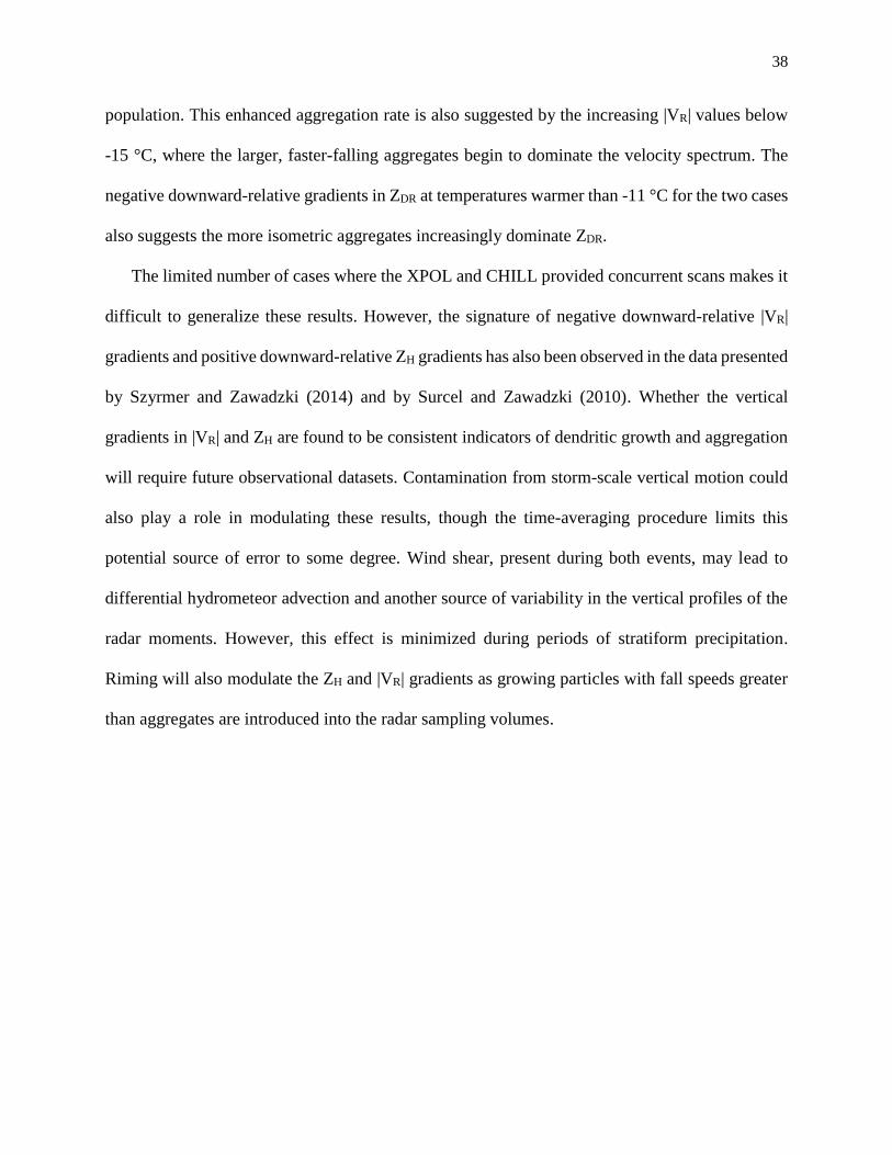
The limited number of cases where the XPOL and CHILL provided concurrent scans makes it
difficult to generalize these results. However, the signature of negative downward-relative |VR|
gradients and positive downward-relative ZH gradients has also been observed in the data presented
by Szyrmer and Zawadzki (2014) and by Surcel and Zawadzki (2010). Whether the vertical
gradients in |VR| and ZH are found to be consistent indicators of dendritic growth and aggregation
will require future observational datasets. Contamination from storm-scale vertical motion could
also play a role in modulating these results, though the time-averaging procedure limits this
potential source of error to some degree. Wind shear, present during both events, may lead to
differential hydrometeor advection and another source of variability in the vertical profiles of the
radar moments. However, this effect is minimized during periods of stratiform precipitation.
Riming will also modulate the ZH and |VR| gradients as growing particles with fall speeds greater
than aggregates are introduced into the radar sampling volumes.
39
Figure 5.1 Time-height profiles of a) ZH, b) ZDR, c) KDP, d) the downward-relative gradient of ZH,
e) the downward-relative gradient of ZDR, and f) the downward-relative gradient of KDP. These
data are based on the CHILL RHI scans along the 220.7° azimuth on 9 March from 10:53 UTC to
21:59 UTC. The yellow dashed contour indicates the height of the RAP model analyzed -15 °C
isotherm while the upper and lower black dashed contours indicate the -20 °C and -10 °C
isotherms, respectively.

40
Figure 5.2 Time-height profiles of a) ZH, b) VR, c) the downward-relative gradient of ZH, d) the
downward-relative gradient of VR. These data are based on the XPOL vertically-pointing scans
taken at the MFS on 9 March from 10:53 UTC to 21:59 UTC. The yellow dashed contour indicates
the height of the -15 °C isotherm while the upper and lower black dashed contours indicate the -
20 °C and -10 °C isotherms, respectively.

41
Figure 5.3 Time-height profiles of a) ZH, b) ZDR, c) KDP, d) the downward-relative gradient of ZH,
e) the downward-relative gradient of ZDR, and f) the downward-relative gradient of KDP. These
data are based on the CHILL RHI scans along the 220.7° azimuth on 20-21 February from
approximately 22:40 UTC to 02:40 UTC. The yellow dashed contour indicates the height of the -
15 °C isotherm while the upper and lower black dashed contours indicate the -20 °C and -10 °C
isotherms, respectively.

42
Figure 5.4 Time-height profiles of a) ZH, b) VR, c) the downward-relative gradient of ZH, d) the
downward-relative gradient of VR. These data are based on the XPOL vertically-pointing scans
taken at the MFS on 20-21 February from approximately 22:20 UTC to 02:20 UTC. The yellow
dashed contour indicates the height of the -15 °C isotherm while the upper and lower black dashed
contours indicate the -20 °C and -10 °C isotherms, respectively.
43
Figure 5.5 Time-averaged profiles of a) downward-relative |VR| gradient, b) downward-relative ZH
gradient, and c) downward-relative ZDR gradient for 20-21 February (solid line) and 9 March
(dashed line). The time-height profiles used to create the time-averaged profiles shown here
correspond to Fig. 5.1 and 5.2 for the 20-21 February profiles and Fig. 5.3 and 5.4 for the 9 March
profiles.

44
CHAPTER 6. ELECTROMAGNETIC SCATTERING CALCULATIONS
Based on the results presented in chapters 4 and 5, there is evidence for the presence of
dendritic growth zones within a number of different cases. Forward modeling, in which the radar
signatures of dendritic ice crystals are simulated, can support or reject whether these ice crystals
are present. In order to represent the populations of ice crystals found in the dendritic growth zone,
PSDs are needed.
Previous studies (e.g., Andrić et al. 2013; Kennedy and Rutledge 2011) have used PSDs either
from a microphysical model or an observational study to calculate the radar observables. However,
these studies failed to fully reproduce the observed radar signatures, suggesting there were errors
in the modeling of the ice crystals or in the PSDs. The variability in the radar signatures near -15
°C shown in chapter 4 suggests there is also variability in the ice crystal PSDs associated with
these signatures.
Therefore, to account for PSD error and variability, a different approach is taken in this study
where the PSDs for ice crystals are determined based on the radar observations, after first
separating out the contributions to the polarimetric variables from aggregates. If these ice crystal
PSDs are physically realistic, then they may provide plausible descriptions of the ice particle size
spectrum for certain polarimetric radar signatures in the dendritic growth zones. The first step
necessary in performing this analysis is to calculate the scattering properties of the individual
crystals with size.
6.1 Description and Monodisperse Distribution Calculations

45
The scattering calculations for pristine ice particles are used based on the ice crystal database
described in Botta et al. (2013) and Lu et al. (2014), which employs the Generalized Multi-particle
Mie (GMM) method. The GMM method involves composing a particle of non-overlapping spheres
and solving the scattering of the collection of spheres analytically. In order for this method to be
accurate, the distribution of mass within the particle must be represented well by the collection of
spheres. Further details can be found in Botta et al. (2013) and Lu et al. (2014).
From the variety of ice crystal morphologies within the database, hexagonal plates and
dendrites were chosen to best represent the likely hydrometeors sampled by the radar, based on
prior work and the observed temperatures. The aspect ratios of these crystals are based on the
empirical formulas in Pruppacher and Klett (1997), adapted from Auer and Veal (1970), shown in
Table 6.1. To get a larger range of possible ice crystal dimensions, the crystal thicknesses were
multiplied by 0.5 for dendrites and by 0.5 and 2.0 for plates. The dendrites in the database have
maximum dimensions (D) of 0.5 mm to 5.65 mm. The maximum dimensions of the plates ranged
from 0.10 mm to 3.27 mm (Lu et al. 2014).
In order to calculate ZDR, ZH, and KDP from the simulated scattering amplitudes, assumptions
about the canting of these ice particles were made. The particles were assumed to be oriented
according to a two-dimensional Gaussian distribution of canting angles with the mean canting
angle set to 0° and the standard deviation (σ) varying from 1° to 20°. Previous studies have found
σ to be between 10°-15° for pristine ice crystals (e.g., Matrosov et al. 2005). The radar observables
for each orientation distribution are then calculated using the angular moments from Ryzhkov et
al. (2011).
The scattering calculations for dendrites with thicknesses of 1.0 and 0.5 times that determined
by the empirical size relationship (hereafter d1.0 and d0.5, respectively) and plates with thickness
46
twice that prescribed by the empirical relationship (hereafter referred to as p2.0) are shown in Fig.
6.1. These calculations use monosdisperse distributions for each crystal corresponding to a total
ZH = 3 dBz (i.e., representative of case 3). As σ increases, ZDR decreases because of the smaller
total projection of the horizontally polarized signal onto the axes of the ice particles’ maximum
dimensions. The largest ice crystals have the lowest KDP values due to their number concentration
being constrained to have a ZH = 3 dBz. Due to Zh (in mm6 m-3) being approximately proportional
to D6, the smallest particles have much larger number concentrations (or total mass) to achieve ZH
= 3 dBz and thus produce KDP values several orders of magnitude higher than the largest particles.
The behavior exhibited by the calculated ZDR is somewhat different between the p2.0 (Fig.
6.1c) and d1.0 (Fig. 6.1b) particles. The dendrites show a minor degree of variance in ZDR with
maximum dimension. For example, the leftmost points with σ = 20° range from about 4.6 dB to
4.8 dB. This variability in ZDR is roughly equal for all other values of σ. The ZDR values for the
plates, however, show a greater range over size with fixed values of σ. For σ = 20°, ZDR ranges
from 2.7 dB for the 0.1-mm crystals to 5.2 dB for the 2.5-mm crystals. The difference in ZDR
between the smallest and largest particles increases to about 4.2 dB for σ = 1°. This relationship
between the maximum dimension of plates and ZDR can be explained by the particles becoming
more oblate with increasing maximum dimension while retaining the same internal distribution of
mass. However, the relative consistency of ZDR with maximum dimension for the dendrites is
likely due to their more complex shape and larger size, resulting in a more heterogeneous
distribution of mass across the particle and thus more complicated scattering behavior.
Based on these results for monodisperse ice crystal particle size distributions (PSDs), only
observed radar signatures with large ZDR can possibly be explained by these calculations alone. In
case 3 above, the peak median ZDR value of 4.5 dB at 3.3 km was associated with a KDP of 0.3 deg

47
km-1 and a ZH of 3 dBz. The scattering calculations for p2.0 show that plates with a maximum
dimension of 0.6 mm, a number concentration ~104 m-3 and σ = 18° best match the observations.
Values of σ closer to 10° result in similar values of KDP and ZDR values around 5.5 dB. Note that
the distribution of ZDR values near 3.3 km ARL (Fig. 4.5a) shows a significant number of points
clustered around 5.0 dB. These values may be a better estimate of the ZDR contribution solely from
pristine ice crystals. Also, the location of the ZDR anomaly near echo top may contain a greater
degree of turbulence and thus more enhanced fluttering of particles, which may increase σ values
over those established in previous studies.
These simple monodisperse PSDs of plates may therefore provide reasonable correspondence
with the observations from case 3. The number concentration (~104 m-3) falls within the range of
observations found in Heymsfield et al. (2013) for temperatures between -15 °C and -20 °C (their
Fig. 4). The other cases described in Chapter 3 were associated with lower ZDR observations and
thus require the addition of a separate class of hydrometeors to decrease the total ZDR.
Monodisperse PSDs are also less physically realistic for a population of ice crystals in a more
mature stage of development when aggregation may play a more considerable role and differential
depositional growth conditions may widen the particle size spectrum.
6.2 PSD retrieval with Mixtures of Aggregates
In this study, we assume that only aggregates and pristine ice crystals are present in the radar
sampling volumes. Therefore, the radar-observed values of ZH, ZDR, and KDP are each composed
of contributions from ice crystals and aggregates. Since the pristine ice crystal PSD is desired, the
contributions to the polarimetric variables from the aggregates must be separated from that of the
ice crystals. This analysis requires knowledge of the ZDR and KDP values associated with a
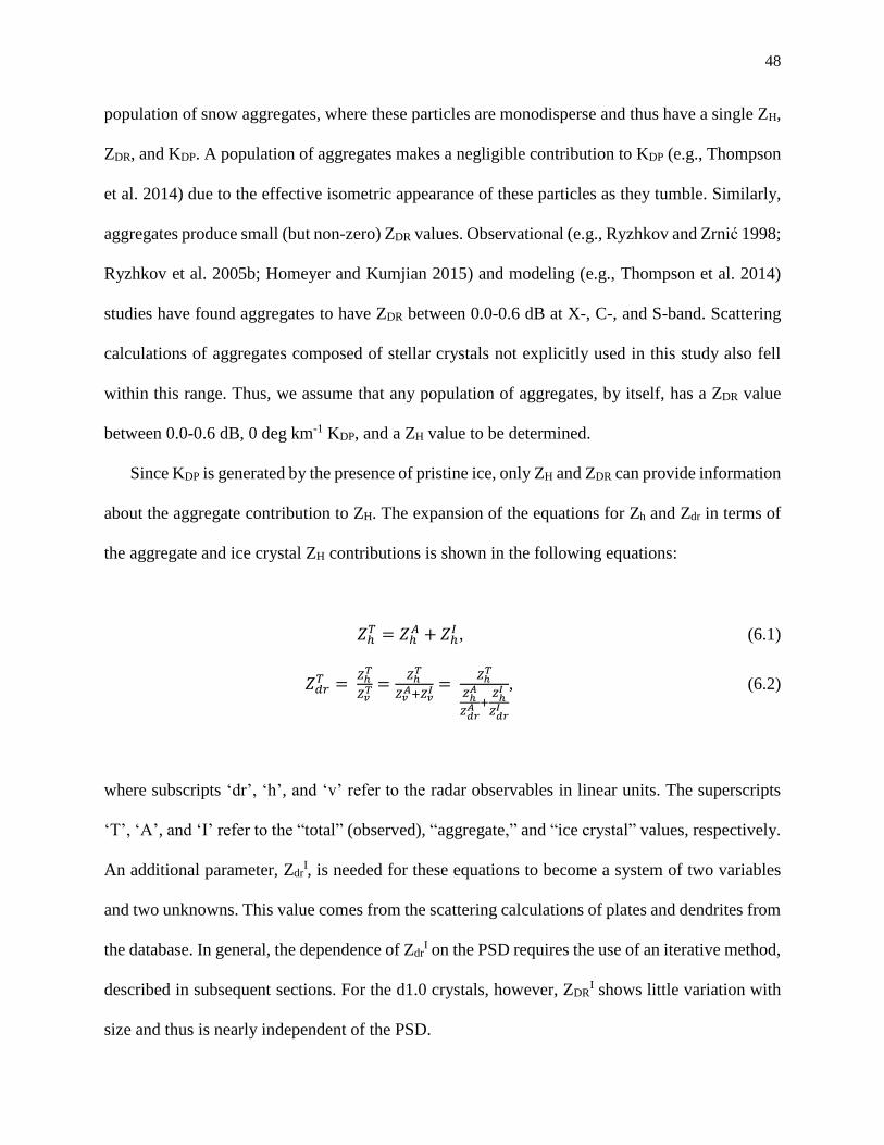
48
population of snow aggregates, where these particles are monodisperse and thus have a single ZH,
ZDR, and KDP. A population of aggregates makes a negligible contribution to KDP (e.g., Thompson
et al. 2014) due to the effective isometric appearance of these particles as they tumble. Similarly,
aggregates produce small (but non-zero) ZDR values. Observational (e.g., Ryzhkov and Zrnić 1998;
Ryzhkov et al. 2005b; Homeyer and Kumjian 2015) and modeling (e.g., Thompson et al. 2014)
studies have found aggregates to have ZDR between 0.0-0.6 dB at X-, C-, and S-band. Scattering
calculations of aggregates composed of stellar crystals not explicitly used in this study also fell
within this range. Thus, we assume that any population of aggregates, by itself, has a ZDR value
between 0.0-0.6 dB, 0 deg km-1 KDP, and a ZH value to be determined.
Since KDP is generated by the presence of pristine ice, only ZH and ZDR can provide information
about the aggregate contribution to ZH. The expansion of the equations for Zh and Zdr in terms of
the aggregate and ice crystal ZH contributions is shown in the following equations:
𝑍ℎ𝑇 = 𝑍ℎ
𝐴 + 𝑍ℎ𝐼 , (6.1)
𝑍𝑑𝑟𝑇 =
𝑍ℎ𝑇
𝑍𝑣𝑇 =
𝑍ℎ𝑇
𝑍𝑣𝐴+𝑍𝑣
𝐼 = 𝑍ℎ
𝑇
𝑍ℎ𝐴
𝑍𝑑𝑟𝐴 +
𝑍ℎ𝐼
𝑍𝑑𝑟𝐼
, (6.2)
where subscripts ‘dr’, ‘h’, and ‘v’ refer to the radar observables in linear units. The superscripts
‘T’, ‘A’, and ‘I’ refer to the “total” (observed), “aggregate,” and “ice crystal” values, respectively.
An additional parameter, ZdrI, is needed for these equations to become a system of two variables
and two unknowns. This value comes from the scattering calculations of plates and dendrites from
the database. In general, the dependence of ZdrI on the PSD requires the use of an iterative method,
described in subsequent sections. For the d1.0 crystals, however, ZDRI shows little variation with
size and thus is nearly independent of the PSD.

49
Equations (6.1) and (6.2) can be solved for the contribution to Zh by ice crystals, ZhI, using the
observed values of ZhT and Zdr
T, ZdrI from the ice crystal scattering calculations, and an assumption
about ZdrA. The resulting equation for ZH
I is shown below,
𝑍ℎ𝐼 = 𝑍ℎ
𝑇 (𝑍𝑑𝑟
𝐼
𝑍𝑑𝑟𝑇 ) (
𝑍𝑑𝑟𝑇 −𝑍𝑑𝑟
𝐴
𝑍𝑑𝑟𝐼 −𝑍𝑑𝑟
𝐴 ), (6.3)
where ZHI varies from 0 dBz to ZH
T, depending on how close ZDRT is to ZDR
I and ZDRA. ZH
I as a
function of ZDRT and ZH
T is shown in Fig. 6.2 for the labeled values of ZDRI and ZDR
A. The
calculated value of ZHI can now constrain one of the parameters used to define a particular PSD.
Generalized gamma distributions can be used to model these PSDs and are defined by the
equation N(D) = N0Dµexp(-λD), where N0 is the intercept parameter, μ is the shape parameter, and
λ is the slope parameter. The case where µ = 0 is the exponential distribution, which will be used
primarily herein. Another commonly used version of the generalized gamma distribution is where
µ = 2, hereafter referred to as the gamma distribution. Because two parameters are needed to define
these PSDs (λ and N0), another constraining radar moment is required. Since KDPT will be roughly
equal to KDPI due to the minimal contribution from aggregates, KDP
I provides the second constraint
on the PSD. A variety of λ and N0 values can then be used to calculate KDPI and ZH
I for various ice
crystal PSDs. The PSD with λ and N0 that produces KDPI and ZH
I matching the constraining KDPI
and ZHI values can thus be determined. In order for the λ and N0 that produce the given KDP
I and
ZHI constraints to be found, a method for calculating the polarimetric variables from a PSD is
needed.
To determine the ZH and KDP for a PSD of ice crystals from the database, the ZH and KDP values
of single crystals are used. These intrinsic ZH and KDP values for each crystal size in the database

50
are found by dividing the monodisperse ZH (equal to 3 dBz for all the crystals shown in Fig. 6.1)
and KDP values at each size by their corresponding number concentration. The number of particles
contained within each crystal size bin (the increment between consecutive crystal sizes) given by
the PSD is then multiplied by the intrinsic ZH and KDP. The sum of the ZH and KDP values
contributed by each size gives ZHI and KDP
I. As mentioned earlier, the database has crystals
available only for a set of fixed sizes. In order to use exponential or gamma distributions to model
ice PSDs, these sizes must approximate well the contribution to the radar variables over the full,
continuous distribution spanning all possible maximum dimensions. For the ice particles with
maximum dimensions > 0.5 mm, dendrites are used. Plate crystals are used for sizes between 0.1
mm and 0.5 mm. This is also physically realistic because plate crystals are the primary habit
preceding dendritic growth. The exact size where plates begin to show characteristics of dendrites
depends on the specific growth conditions.
For the ice crystals where there is variation in ZDR with size, ZDRI, and thus ZH
I, is dependent
on the PSD. Therefore, an iterative procedure for determining ZDRI is needed. This process (shown
schematically in Fig. 6.3) uses a first guess for ZDRI to find an initial estimate of ZH
I, using the
procedure described earlier. This ZHI estimate is then used with KDP
I to make an initial estimate of
N0 and λ. An updated value of ZDRI is then calculated from these PSD parameters, allowing for
ZHI, and thus N0 and λ to be further refined. This step is depicted as the outermost arrow in Fig.
6.3 extending from the ice PSD parameters to the ZDRI value. Only a few iterations are needed for
the N0 and λ values to converge.
Figure 6.4 shows the relationship between the PSD parameters for the combination of p1.0 and
d1.0 crystals and the resulting KDPI and ZH
I values. The intersection of these two curves gives the
N0 and λ values needed to match the radar observations. Both KDPI and ZH
I increase with increasing
51
N0 as a larger number of ice particles at all sizes are present. Increasing λ with constant N0 leads
to a decrease in both polarimetric variables as both the total number concentration and median
particle size decrease. For a constant λ, increasing N0 leads to an increase in KDPI and ZH
I, with the
KDPI contours becoming more tightly packed. The relatively small angles between the KDP
I and
ZHI curves in Fig. 6.4 imply a high sensitivity of these values to both PSD parameters. This
sensitivity is explored further in chapter 7.
The PSDs resulting from this methodology are shown in Table 6.2, along with the observed
radar variables associated with each case. The retrieved N0 values for the diverse set of radar
signatures vary about an order of magnitude. A large range in λ is evident as well, with a ~5.3 mm-
1 difference between high and low values. The ZHI, ZDR
I, and KDPI computed from the retrieved
PSD parameters for each case combined with the derived ZHA provide exact matches with the
radar-observed values. Thus, unlike previous studies (Kennedy and Rutledge 2011; Andrić et al.
2013; Bechini et al. 2013), the PSDs derived herein are consistent with the suite of polarimetric
radar observations.
The retrieved PSD for the signature observed in case 2 (cf. Fig. 4.3) is plotted in Fig. 6.5. A
relatively high number concentration of smaller particles is derived for this case, with λ = 3.29
mm-1. The greatest contributions to KDPI from this PSD come from ice crystals with maximum
dimensions between ~0.5-1.5 mm. These crystals have moderate values of normalized KDP, but
are in sufficiently high concentration, and thus have a sufficiently large mass, to produce much of
the observed enhancement. At greater maximum dimensions, the marginal contributions to KDPI
decrease substantially. In contrast, dendrites with maximum dimensions between 1.2-1.6 mm
contribute the most towards ZHI with a slower decrease in the marginal contributions to ZH
I with
size. This is due to ZH depending more strongly on particle size.
52
For case 1 (cf. Fig. 3.5), a shallower PSD is retrieved (Fig. 6.6). In this PSD, the greatest
contribution to KDPI comes from the dendrites with maximum dimensions of ~1.5 mm. Relative to
the previous example, a slower decrease with size is seen in the marginal contribution to KDPI. The
greatest contribution to ZHI, however, comes from dendrites with maximum dimensions between
3-4 mm, due to their increased concentrations and the size dependence of ZHI.
The largest λ was observed for the case with largest ZDRT (case 3). As mentioned in the previous
section, these radar observations correspond fairly well to a monodisperse PSD of plates having a
maximum dimension of 0.5 mm. Only the p2.0 crystal type was used here because the lower
normalized ZDRI values of these crystals require lesser ZH
A values to match ZDRT. This reflects the
likely dearth of aggregation ongoing with plate crystals near echo top. The relatively low ZHI and
modest KDPI for these crystals resulted in a slope parameter of 7.13 mm-1 (Fig. 6.7). The sharp
peak in the KDPI contribution centered on the 0.5-mm crystal size bin suggests this PSD behaves
similarly to the monodisperse distribution for plates of this size.

53
Table 6.1. Description of the plates and dendrites from the database shown in Botta (2013).
Adapted from Lu et al. (2014). D is the maximum dimension of the particles, while h is the
particle thickness and is orthogonal to D.
D (mm) h(cm), D(cm) Thickness Factor
Dendrites 0.5-5.65 h = 9.022 x 10⁻³D0.377 0.5,1.0
Plates 0.1-3.27 h = 1.41 x 10⁻²D0.474 0.5,1.0,2.0
Table 6.2. Exponential ice PSDs determined from the radar observations listed in columns 2, 5
and 6. An aggregate ZDR of 0.3 dB, an aggregates KDP of 0 deg km-1, and σ = 15° are assumed
for these calculations.
Case ZHT
(dBz)
ZHI
(dBz)
ZHA
(dBz)
ZDRT
(dB)
KDPT/KDP
I
(deg km-1)
N0
(m-3 mm-1)
λ
(mm-1)
Crystal
Types
2/21/13 00:58 UTC 15 10.2 13.25 1.5 1.3 2.77 x 10⁵ 3.21 p1.0,d1.0
Case 1:
3/9/13 12:49 UTC
23 16.1 22.01 1 1.6 5.91 x 10⁴ 1.87 p1.0,d1.0
Case 2:
3/9/13 19:51 UTC
13 7.9 11.39 1.4 0.8 1.84 x 10⁵ 3.29 p1.0,d1.0
Case 3:
4/9/13 19:40 UTC
3 2.5 -6.64 4.5 0.3 3.85 x 10⁵ 7.13 p2.0
54
Figure 6.1. Scattering calculations for monodisperse populations of a) dendrites with one half the
reference thickness, b) dendrites of the reference thickness and c) plates twice the reference
thickness based on the empirical relationships found in Auer and Veal (1970). The ZH values for
all data points are 3 dBz. The numbers to the left of the data indicate the maximum dimension (in
mm) and number concentration (in m-3) for the size class of ice particles, respectively. The color
of the points differentiate the crystals sizes for which the scattering calculations are performed.
The size of the markers indicates the canting angle distribution width (σ) with the largest markers
equal to 20° and the smallest markers equal to 1°.
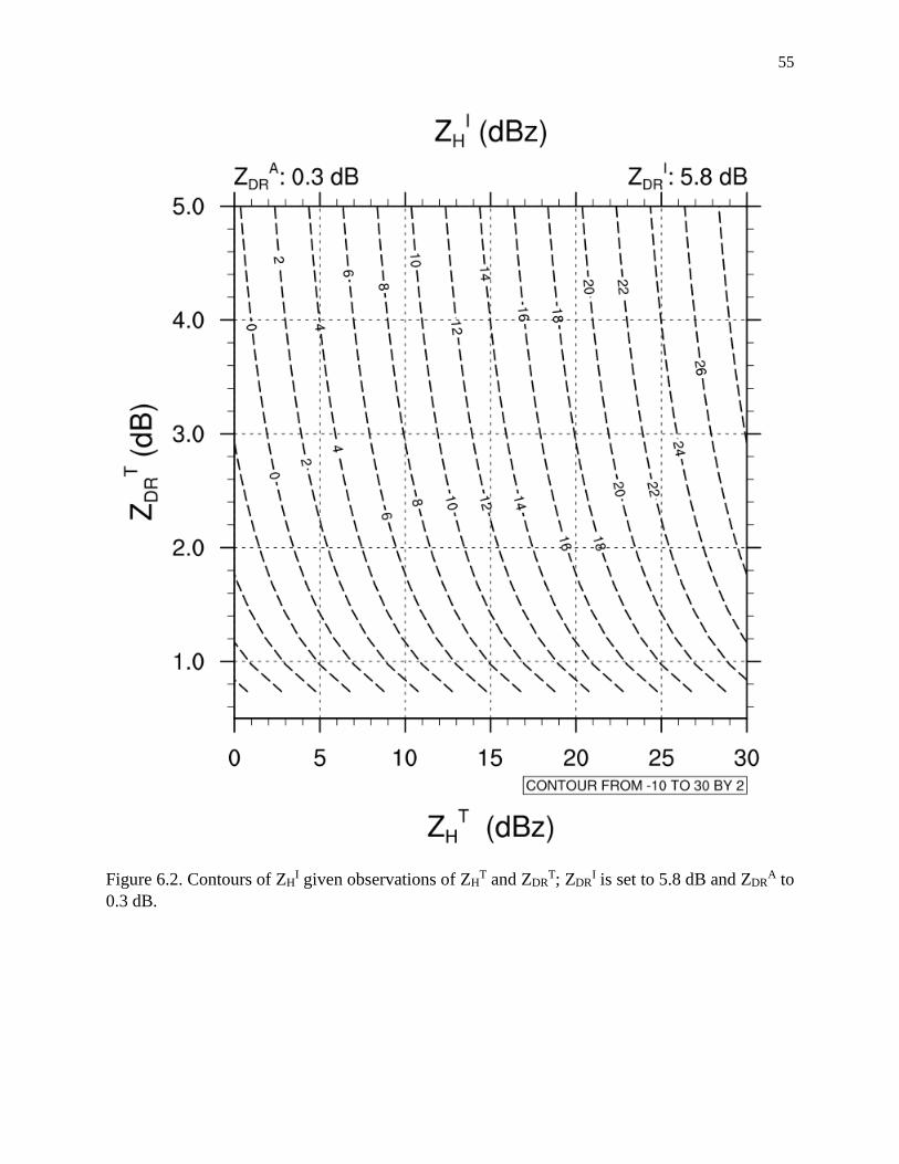
55
Figure 6.2. Contours of ZHI given observations of ZH
T and ZDRT; ZDR
I is set to 5.8 dB and ZDRA to
0.3 dB.
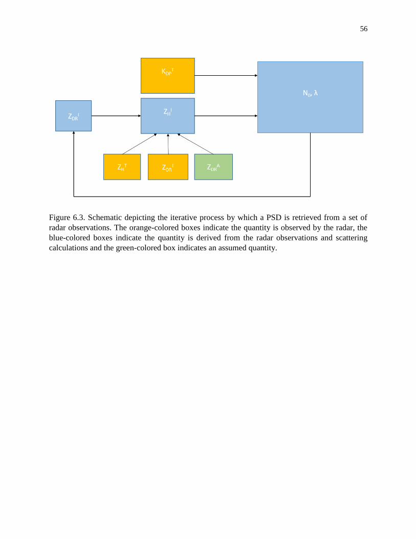
56
Figure 6.3. Schematic depicting the iterative process by which a PSD is retrieved from a set of
radar observations. The orange-colored boxes indicate the quantity is observed by the radar, the
blue-colored boxes indicate the quantity is derived from the radar observations and scattering
calculations and the green-colored box indicates an assumed quantity.

57
Figure 6.4. Contours of KDPI (blue) and the ZH
I (red) contribution from ice as a function of the
slope and intercept parameters for PSDs of exponential form. ZHI is contoured every 2 dBz from
0 dBz to 20 dBz.

58
Figure 6.5. Plot of the number concentration per size (maroon), marginal contribution to ZhI
(orange) and marginal contribution to KDPI (blue) corresponding to case 2; the exponential PSD
for this case has N0 = 1.84x10⁵ m-3 mm-1 and λ= 3.29 mm-1. Ice particles to the left of the red
dashed line are of type p1.0 and of type d1.0 to the right.

59
Figure 6.6. Plot of the number concentration per size (maroon), marginal contribution to ZhI
(orange) and marginal contribution to KDPI (blue) corresponding to case 1; the exponential PSD
for this case has N0 = 5.91x10⁴ m-3 mm-1 and λ= 1.87 mm-1. Ice particles to the left of the red
dashed line are of type p1.0 and of type d1.0 to the right.

60
Figure 6.7. Plot of the number concentration per size (maroon), marginal contribution to ZhI
(orange) and marginal contribution to KDPI (blue) corresponding to case 3; the exponential PSD
for this case has N0 = 3.85x10⁵ m-3 mm-1 and λ= 7.13 mm-1. The ice particles used here are all of
type p2.0.
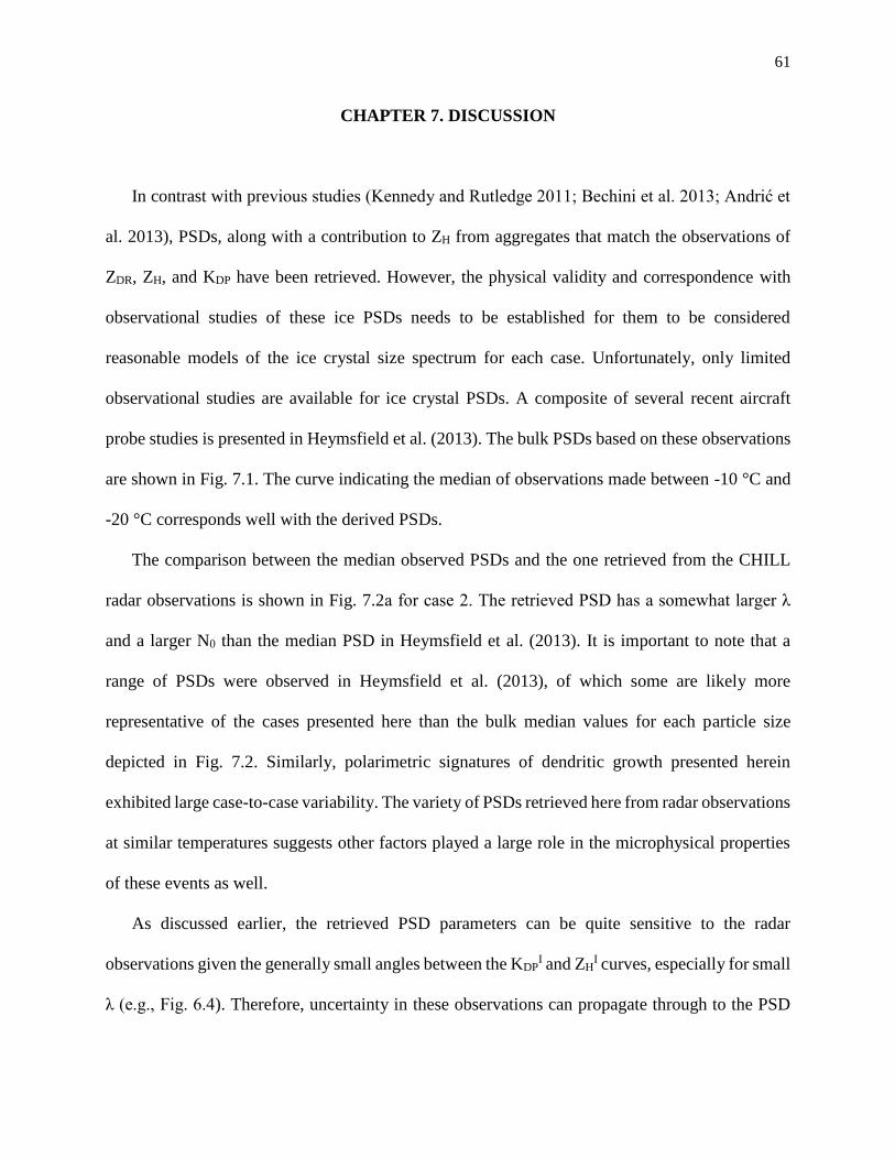
61
CHAPTER 7. DISCUSSION
In contrast with previous studies (Kennedy and Rutledge 2011; Bechini et al. 2013; Andrić et
al. 2013), PSDs, along with a contribution to ZH from aggregates that match the observations of
ZDR, ZH, and KDP have been retrieved. However, the physical validity and correspondence with
observational studies of these ice PSDs needs to be established for them to be considered
reasonable models of the ice crystal size spectrum for each case. Unfortunately, only limited
observational studies are available for ice crystal PSDs. A composite of several recent aircraft
probe studies is presented in Heymsfield et al. (2013). The bulk PSDs based on these observations
are shown in Fig. 7.1. The curve indicating the median of observations made between -10 °C and
-20 °C corresponds well with the derived PSDs.
The comparison between the median observed PSDs and the one retrieved from the CHILL
radar observations is shown in Fig. 7.2a for case 2. The retrieved PSD has a somewhat larger λ
and a larger N0 than the median PSD in Heymsfield et al. (2013). It is important to note that a
range of PSDs were observed in Heymsfield et al. (2013), of which some are likely more
representative of the cases presented here than the bulk median values for each particle size
depicted in Fig. 7.2. Similarly, polarimetric signatures of dendritic growth presented herein
exhibited large case-to-case variability. The variety of PSDs retrieved here from radar observations
at similar temperatures suggests other factors played a large role in the microphysical properties
of these events as well.
As discussed earlier, the retrieved PSD parameters can be quite sensitive to the radar
observations given the generally small angles between the KDPI and ZH
I curves, especially for small
λ (e.g., Fig. 6.4). Therefore, uncertainty in these observations can propagate through to the PSD

62
estimation. To gauge the impact of observational uncertainty on the PSD parameters, 20%
perturbations in ZDRT and KDP
T were imposed on the observations for each case. The percentage
changes due to these modifications can be seen in Table 7.1.
Case 1, which had the highest ZHT and lowest ZDR
T, showed the greatest sensitivity to changes
in ZDRT, whereas case 3 (which had the lowest ZH
T and highest ZDRT) had the smallest percentage
changes. The main impact of these ZDRT perturbations was to change the relative proportions of
ZHT contributed by aggregates and ice crystals. For the 20% decrease in ZDR
T, the ZHI constraint
will decrease due to ice crystals having a high intrinsic ZDRI. As a result, both λ and N0 must
increase to provide higher contributions to KDPI from smaller-sized ice crystals. Perturbing ZDR
T
(and thus the ZHI constraint) has the greatest impact for PSDs with small λ due to the exponential
dependence of the PSD on this parameter.
Perturbations in KDPT had more consistent impacts across the cases compared to the
perturbations in ZDRT. This is due to the ZH
I constraint depending on both ZDRT and ZH
T, while
KDPT (KDP
I) is a direct constraint on the PSD. Increases in KDPT resulted in increases in N0 and λ
of 54-59% and 7-9%, respectively. Both N0 and λ increased due to the greater contribution of
smaller particles needed to produce a larger KDPI with the same ZH
I. Negative perturbations in KDPT
had the inverse effect.
Another source of uncertainty is the assumption of the bulk ZDRA and KDP
A values. Due to the
likely minimal contribution to KDP from aggregates, the resulting changes in PSD parameters will
be very small. However, the assumed ZDRA can have a significant impact on the ZH
I constraint for
the ice crystal PSD. To determine the sensitivity of the PSD parameters to this assumption, PSDs
were determined for each case using ZDRA values of 0.0 dB and 0.6 dB (Table 7.2). Again, resulting
changes in both PSD parameters were largest for case 1, which had the largest ZHT and smallest
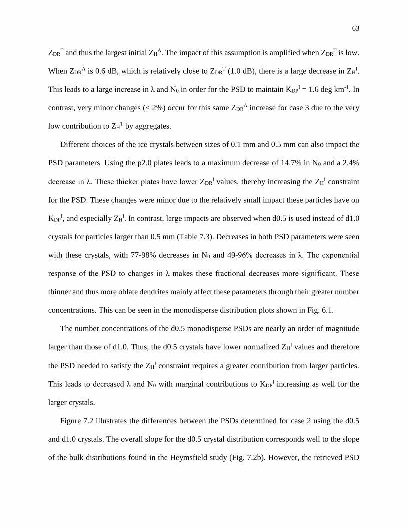
63
ZDRT and thus the largest initial ZH
A. The impact of this assumption is amplified when ZDRT is low.
When ZDRA is 0.6 dB, which is relatively close to ZDR
T (1.0 dB), there is a large decrease in ZHI.
This leads to a large increase in λ and N0 in order for the PSD to maintain KDPI = 1.6 deg km-1. In
contrast, very minor changes (< 2%) occur for this same ZDRA increase for case 3 due to the very
low contribution to ZHT by aggregates.
Different choices of the ice crystals between sizes of 0.1 mm and 0.5 mm can also impact the
PSD parameters. Using the p2.0 plates leads to a maximum decrease of 14.7% in N0 and a 2.4%
decrease in λ. These thicker plates have lower ZDRI values, thereby increasing the ZH
I constraint
for the PSD. These changes were minor due to the relatively small impact these particles have on
KDPI, and especially ZH
I. In contrast, large impacts are observed when d0.5 is used instead of d1.0
crystals for particles larger than 0.5 mm (Table 7.3). Decreases in both PSD parameters were seen
with these crystals, with 77-98% decreases in N0 and 49-96% decreases in λ. The exponential
response of the PSD to changes in λ makes these fractional decreases more significant. These
thinner and thus more oblate dendrites mainly affect these parameters through their greater number
concentrations. This can be seen in the monodisperse distribution plots shown in Fig. 6.1.
The number concentrations of the d0.5 monodisperse PSDs are nearly an order of magnitude
larger than those of d1.0. Thus, the d0.5 crystals have lower normalized ZHI values and therefore
the PSD needed to satisfy the ZHI constraint requires a greater contribution from larger particles.
This leads to decreased λ and N0 with marginal contributions to KDPI increasing as well for the
larger crystals.
Figure 7.2 illustrates the differences between the PSDs determined for case 2 using the d0.5
and d1.0 crystals. The overall slope for the d0.5 crystal distribution corresponds well to the slope
of the bulk distributions found in the Heymsfield study (Fig. 7.2b). However, the retrieved PSD
64
has an N0 roughly one order of magnitude greater than the observed median PSD. For dendrites
with maximum dimensions between about 1.0-2.5 mm, the PSD fitting the d1.0 crystals was closer
in value than that for the d0.5 crystals. This size range also exhibited the greatest contributions to
KDPI and ZH
I for both PSDs.
Finally, fitting the radar observations to a gamma distribution instead of an exponential
distribution also leads to differences in the marginal contributions to the radar observables with
size. The gamma PSD parameters that fit the observations for each case are shown in Table 7.4.
Generally, the gamma PSDs had much lower marginal contributions to the ZHI and KDP
I from the
larger particles than the exponential PSDs, which is expected based on the narrower spectral
shapes. For case 2, lower marginal contributions to ZHI and KDP
I are seen for the smallest ice
crystals as well as those > 2 mm. Dendrites with maximum dimensions between 0.5-2.0 mm
provide larger contributions to KDPI and ZH
I to compensate for the decreased contributions from
the other sizes.
These variable radar signatures and the corresponding derived PSDs provide insights into the
ongoing microphysics during these cases. In case 3, the derived PSD suggests a highly sloped
exponential distribution is present with the ice particles clustered within a narrow range of sizes.
This suggests that the early stages of depositional growth was occurring, producing a relatively
narrow distribution of small crystals yet to exhibit dendritic characteristics, and thus yet to exhibit
any substantial degree of aggregation.
The stratiform, upslope-induced case 2 also had a relatively steep slope parameter. However,
the contribution to ZHT from aggregates was greater than that produced by the dendrites. This
suggests a relatively low number concentration of aggregates are present which provide an
65
adequate ZHA contribution yet also allow a large enough concentration of small, oblate particles to
exist and match the KDP and ZDR observations.
A much larger contribution to ZHT from aggregates was determined for case 1. The λ value for
this exponential distribution was shallower than the previous two cases, indicating a much larger
weight towards the largest dendrites. This also suggests that many of smallest crystals in the
distribution had been collected by the larger aggregates. The convective appearance to the radar
echoes in this case, along with the elevated ZHT values, suggest a stronger updraft in the cloud that
could have allowed for a larger growth of dendrites via vapor deposition and thus more efficient
aggregation. Additionally, the analysis in chapter 5.1 suggests that rimed ice crystals may have
also been present. This complicates the interpretation of these radar observations, where riming
could differentially alter the aspect ratios comprising a preexisting ice PSD.
Microphysical models of ice processes require, among other parameters, knowledge about ice
crystal and snow aggregate fall speeds. However, there is a large amount of uncertainty in these
values given the difficulties in observing such properties of real ice particles in the atmosphere.
The signature observed by the vertically pointing XPOL, associated with the dendritic growth and
aggregation of these crystals, can help constrain the range of fall speeds and other microphysical
parameters used in the models.
For the limited number of cases presented in this study, the maximum downward-relative
vertical gradient in ZH was consistently between 3 dB km-1 and 10 dB km-1 and found near the
dendritic growth zone. Maximum ZH gradients in stratiform precipitation events were found by
Surcel and Zawadzki (2010) and Bechini et al. (2013) to be within this range of values as well. If
the downward-relative gradient in ZH falls between 3 dB km-1 and 10 dB km-1 near the dendritic
growth zone for a large sample of stratiform precipitation events, the uncertainty in the treatment

66
of aggregation of dendrites in numerical models can be constrained. Similarly, if found to be
consistent over a large number of cases, the negative downward-relative gradient in |VR| near the
dendritic growth zone, as presented in this study, can be used to reduce the uncertainty in the fall
speeds of aggregates and dendrites. Model simulations of aggregation and vapor deposition in
environments conducive for dendritic growth can be compared with the radar observations using
forward operators for ZH and |VR|. Large deviations between the simulated and constraining ZH
and |VR| gradient values will indicate significant errors in the model parameters. These parameters
(such as fall speed) can then be tuned to better match the ZH and |VR| gradient constraints.

67
Table 7.1. Percentage changes in N0 and λ with respect to the values shown in table 6.2, for 20%
perturbations in ZDR and KDP.
+20% Kdp Percentage Change in N0 Percentage Change in λ
2/21/13 00:58 UTC 56.3 8.4
Case 1: 3/9/13 12:49 UTC 59.2 9.1
Case 2: 3/9/13 19:51 UTC 56.0 8.2
Case 3: 4/9/13 19:40 UTC 53.8 7.0
Mean 56.3 8.2
-20% Kdp
2/21/13 00:58 UTC -42.6 -9.7
Case 1: 3/9/13 12:49 UTC -44.0 -10.7
Case 2: 3/9/13 19:51 UTC -42.4 -9.7
Case 3: 4/9/13 19:40 UTC -40.8 -7.9
Mean -42.4 -9.5
+20% Zdr
2/21/13 00:58 UTC -24.5 -8.1
Case 1: 3/9/13 12:49 UTC -30.6 -11.2
Case 2: 3/9/13 19:51 UTC -25.0 -8.5
Case 3: 4/9/13 19:40 UTC -13.5 -3.9
Mean -23.4 -7.9
-20% Zdr
2/21/13 00:58 UTC 44.4 11.8
Case 1: 3/9/13 12:49 UTC 62.4 16.0
Case 2: 3/9/13 19:51 UTC 45.1 12.2
Case 3: 4/9/13 19:40 UTC 22.9 5.9
Mean 43.7 11.5

68
Table 7.2. Percentage changes in N0 and λ with respect to the values shown in table 3, for
aggregate ZDR values of 0.0 and 0.6 dB.
Aggregate ZDR = 0.0 dB Percentage Change in N0 Percentage Change in λ
2/21/13 00:58 UTC -21.7 -7.2
Case 1: 3/9/13 12:49 UTC -38.2 -14.4
Case 2: 3/9/13 19:51 UTC -23.9 -7.9
Case 3: 4/9/13 19:40 UTC -1.3 -0.4
Mean -27.9 -9.8
Aggregate ZDR = 0.6 dB
2/21/13 00:58 UTC 38.6 10.6
Case 1: 3/9/13 12:49 UTC 114.9 26.7
Case 2: 3/9/13 19:51 UTC 44.0 11.9
Case 3: 4/9/13 19:40 UTC 1.8 0.6
Mean 65.8 16.4
Table 7.3. Percentage changes in N0 and λ with respect to the values shown in table 3, for crystal
types of p1.0 and d0.5. No modification of crystal type was imposed on the 9 April case.
Crystal Types: p1.0,d0.5 Percentage Change in N0 Percentage Change in λ
2/21/13 00:58 UTC -77.83 -49.84
Case 1: 3/9/13 12:49 UTC -97.83 -95.72
Case 2: 3/9/13 19:51 UTC -76.85 -48.63
Case 3: 4/9/13 19:40 UTC
Mean -84.17 -64.73

69
Table 7.4. Gamma ice PSDs determined from the radar observations listed in columns 2, 5 and 6.
An aggregate ZDR of 0.3 dB and σ = 15° are assumed for these calculations.
Case ZHT
(dBz)
ZHI
(dBz)
ZHA
(dBz)
ZDRT
(dB)
KDPT/KDP
I
(deg km-1)
N0
(m-3 mm-1)
λ
(mm-1)
Crystal
Types
2/21/13 00:58 UTC 15 10.2 13.25 1.5 1.3 2.08 x 10⁶ 4.97 p1.0,d1.0
Case 1:
3/9/13 12:49 UTC
23 16.1 22.01 1 1.6 1.43 x 10⁵ 2.88 p1.0,d1.0
Case 2:
3/9/13 19:51 UTC
13 7.9 11.39 1.4 0.8 1.44 x 10⁶ 5.08 p1.0,d1.0
Case 3:
4/9/13 19:40 UTC
3 2.5 -6.64 4.5 0.3 9.67 x 10⁶ 10.4 p2.0
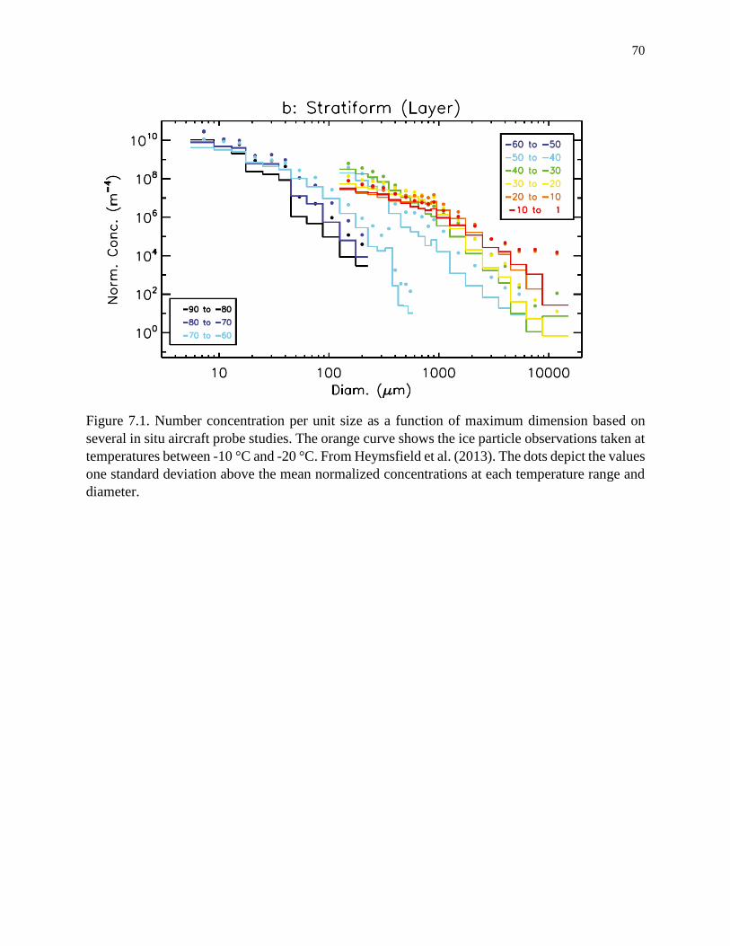
70
Figure 7.1. Number concentration per unit size as a function of maximum dimension based on
several in situ aircraft probe studies. The orange curve shows the ice particle observations taken at
temperatures between -10 °C and -20 °C. From Heymsfield et al. (2013). The dots depict the values
one standard deviation above the mean normalized concentrations at each temperature range and
diameter.

71
Figure 7.2. Plots of the number concentration per size (maroon), marginal contribution to Zh
(orange) and marginal contribution to KDP (blue) for a) particles of type p2.0 and d1.0 and b) type
p2.0 and d0.5 corresponding to case 2. The maroon dashed lines shows the bulk PSD observations
adapted from the Heymsfield et al. (2013) study (Fig. 7.1).

72
CHAPTER 8. CONCLUSIONS
X-band polarimetric and vertically-pointing radar observations collected during several winter
storm events in northern Colorado were analyzed, with particular focus on the signatures found
within regions favored for dendritic growth. A large variability in the observed ZH, ZDR, and KDP
was found. This variability may be partially explained by the differing meteorological conditions
found between and during each event. Periods of significant upslope flow tended to be associated
with more stratiform precipitation and, at times, substantial ZDR enhancements. Features with a
more convective appearance mostly developed with less significant low-level upslope flow. These
cases often exhibited larger ZH but smaller ZDR (indicative of more aggregation), yet large KDP
enhancements suggesting a sizeable population of dendritic crystals. This could include both rapid
growth of dendrites in large supersaturations and/or a larger number concentration of dendrites.
Likely due to aggregation, ZDR generally was negatively correlated to ZH, with the highest ZDR
observed with lower ZH. Enhancements in KDP were observed within regions of elevated ZDR
and/or elevated ZH. Since KDP is related to both the total mass and aspect ratio of a sample of
hydrometeors, increases in ZH and/or ZDR can increase its value. The most significant
enhancements, however, were associated with increased ZH. The addition of aggregates will leave
KDP relatively unchanged while decreasing the observed ZDR.
Negative downward-relative gradients in |VR| were observed by the vertically pointing XPOL
near the dendritic growth zone. These values are thought to be related to the onset of dendritic
characteristics during vapor depositional growth. Another persistent signature found near -15 °C
was the maximum in the profile of the downward-relative ZH gradient. These increased ZH
gradients support a maximum in the aggregation rate at this temperature level and provide further
73
evidence for the presence of dendrites due to the enhanced collection efficiencies of these particles.
The greater variation in fall speed between dendrites and aggregates also increases the aggregation
rate. Values of the downward-relative gradient in ZDR were positive at temperatures above -11 °C
and negative at warmer temperatures. This indicates that dendrites growing through vapor
deposition increase ZDR initially, before aggregation dominates the snow growth process. This
lowers ZDR as mass is transferred from the oblate dendrite population to the more isometric
aggregates.
Scattering calculations were performed using the GMM method, with ZH, ZDR, and KDP
calculated using realistic assumptions about the canting behavior of the ensemble of particles. A
monodisperse distribution of plate-like crystals matched relatively well to the observed
polarimetric radar signatures for a case of observed large ZDR. The slope and intercept parameters
for exponential and gamma distributions were retrieved from the radar observations for a variety
of cases. The resulting PSDs corresponded well to previously reported aircraft probe
measurements of ice PSD. The range of PSDs retrieved from the highly variable radar signatures
suggest that these distributions are plausible models to characterize ice crystal size distributions,
given the presence of aggregates. Further evidence these PSDs are physically realistic is that the
property of observed ZDR being positively correlated to λ (Kennedy and Rutledge 2011) is satisfied.
The sensitivity of the derived PSDs to the radar observations, the crystal types used in the
scattering calculations, and assumptions about the scattering properties of aggregates was tested.
The aspect ratio of dendrites made significant impacts on the calculated radar observables and thus
the retrieved PSDs. Electromagnetic scattering calculations for dendrites with aspect ratios that
depend on environmental growth conditions (e.g., Harrington et al. 2013; Sulia et al. 2013, 2014)
may determine PSDs constrained by the radar observations that better fit the limited observational
74
studies of ice PSDs. This also underscores the need for ice crystal observations to better constrain
axis ratio relationships for dendritic and plate-like crystals.
Some information about the microphysical processes associated with certain polarimetric radar
signatures can be inferred. If conditions are unfavorable for riming (i.e., weak vertical motion), ZH
and ZDR can be used to determine the relative contributions of aggregates and ice crystals to the
observed ZH. Enhanced values of KDP in these regions likely suggest that these aggregates rapidly
grow through the collection of dendrites. The greater the observed values of KDP, the greater the
rate of dendritic growth and thus the greater the efficiency in aggregate growth. The PSDs derived
using ZH, ZDR, and KDP can also be compared to gain some information about the growth of snow
through aggregation. For example, shallower slopes indicate collection of the smallest ice particles
by the larger aggregates. The use of scattering calculations of aggregates composed of pristine ice
crystals may be useful in further understanding aggregation processes.
The polarimetric signature of elevated KDP, increasing ZH, and decreasing ZDR towards the
ground, found in the ice-producing region of clouds, is related to the presence of dendritic ice
crystals. Thus, regions where these crystals may be growing can be identified using polarimetric
radar. Further confidence about the presence of these dendrites can be attained if this signature is
observed in a layer saturated with respect to liquid and with temperatures near -15 °C. Due to the
rapid aggregation of these dendrites, these radar observations may be useful in indicating the
occurrence of enhanced snowfall rates.
75
APPENDIX A. ALTERNATIVE KDP ESTIMATION PROCEDURE
In regions where ΦDP is particularly noisy, often where ZH is relatively low, the WC09
estimation procedure sets KDP to 0 deg km-1. Substantial ZDR enhancements due to the presence of
pristine ice crystals at these locations may therefore be incorrectly associated with KDP values close
to 0 deg km-1. In order to better quantify the KDP associated with these ZDR and ZH values, an
alternate method for estimating KDP is introduced. Since this procedure is applied in radar scans
exclusively sampling ice particles, no folding of ΦDP occurs. Also, the backscatter differential
phase shift is considered small, given the high probability that the particles in these high-noise
regions of the echo likely satisfy the Rayleigh approximation.
The first step in this method is removing the data containing primarily noise. A gate is
considered noise when it has a normalized coherent power (NCP) value < 0.4. NCP is a measure
of the predictability of the phase between pulses (Dixon and Hubbert 2012), where values near
one are considered to be mostly signal and those near zero mostly noise. After masking the gates
of high noise, a low-pass range filter is applied to the ΦDP field. The Lanczos filter (Duchon 1979)
was used in this case. This filter is computed using the Fourier transform of a rectangular function
in frequency space and a factor of “sigma,” which minimizes the Gibbs oscillations that occur with
Fourier representations of discrete data. Once the filter is calculated using 2n+1 gates, the resulting
weights can be applied to the range profile of ΦDP. At each gate j, a weighted average of the ΦDP
values from gate j-n to j+n is calculated using the weights determined by the filter. This filtered
value of ΦDP at gate j can only be determined if none of the gates from j-n to j+n have been flagged
as noise.
76
The low-pass cut-off (the width of the rectangular response function) used in this case is the
frequency of oscillations in the KDP field estimated using the WC09 method, corresponding to
approximately 1 peak every 53 gates. Thirty-one points (n = 15) were used to create the Lanczos
filter weights. Gates close to the radar and near echo top with less than 15 ΦDP values at greater
and/or lesser ranges were removed. A linear regression centered on each gate was used to calculate
the slope of the filtered ΦDP profile. While this scheme decreases the overall number of KDP
estimates, estimates are now provided for some of the gates previously flagged as noise (and thus
set to zero) in the WC09 algorithm.
The gates for which estimates of KDP were originally provided (i.e., regions of low noise) by
the WC09 scheme are well correlated with those using this estimation procedure. A comparison
of the vertical profiles of KDP (as in Fig. 4.5b) estimated using the alternate and WC09 methods is
shown in Fig. A1. Below 2.8 km ARL, the median KDP values are nearly identical with slightly
narrower widths and similar shapes to the distributions seen in the alternate KDP estimation.
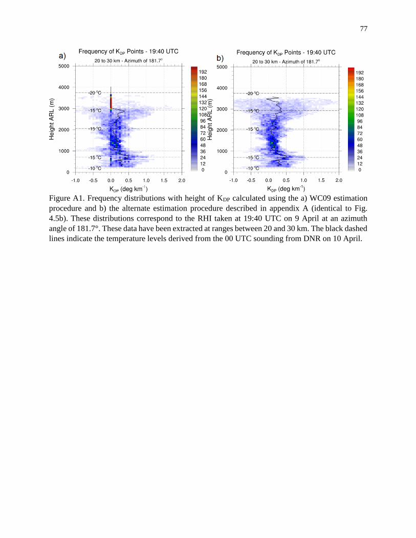
77
Figure A1. Frequency distributions with height of KDP calculated using the a) WC09 estimation
procedure and b) the alternate estimation procedure described in appendix A (identical to Fig.
4.5b). These distributions correspond to the RHI taken at 19:40 UTC on 9 April at an azimuth
angle of 181.7°. These data have been extracted at ranges between 20 and 30 km. The black dashed
lines indicate the temperature levels derived from the 00 UTC sounding from DNR on 10 April.
78
REFERENCES
Andrić, J., M. R. Kumjian, D. S. Zrnić, J. M. Straka, and V. M. Melnikov, 2013: Polarimetric
signatures above the melting layer in winter storms: An observational and modeling Study. J.
Appl. Meteor. Climatol., 52, 682-700.
Auer, A. H. and D. L. Veal, 1970: The dimension of ice crystals in natural clouds. J. Atmos. Sci.,
27, 919–926.
Aydin, K. and T. A. Seliga, 1984: Radar polarimetric backscattering properties of conical
graupel. J. Atmos. Sci., 41, 1887-1892.
Bailey, M. P., and J. Hallett, 2009: A comprehensive habit diagram for atmospheric ice crystals:
Confirmation from the laboratory, AIRS II, and other field studies. J. Atmos. Sci., 66, 2888-2899.
Bechini, R., L. Baldini, and V. Chandrasekar, 2013: Polarimetric radar observations in the ice
region of precipitating clouds at C-band and X-band radar frequencies. J. Appl. Meteor.
Climatol., 52, 1147-1169.
Botta, G., K. Aydin, and J. Verlinde, 2013: Variability in millimeter wave scattering properties
of dendritic ice crystals. J. Quant. Spectrosc. Radiat. Transfer, 131, 105-114.
Brandes E. A., K. Ikeda, G. Thompson, and M. Schönhuber, 2008: Aggregate terminal
velocity/temperature Relations. J. Appl. Meteor. Climatol., 47, 2729-2736.
Bringi V. N., R. M. Rasmussen, and J. Vivekanandan, 1986: Multiparameter radar measurements
in Colorado convective storms. Part I: Graupel melting studies. J. Atmos. Sci., 43, 2545-2563.
Bringi, V. N., and V. Chandrasekar, 2001: Polarimetric Doppler Weather Radar: Principles and
Applications. Cambridge University Press, 636 pp.
Brown, J. M., and Coauthors, 2011: Improvement and testing of WRF physics options for
application to Rapid Refresh and High Resolution Rapid Refresh. Preprints, 14th Conf. on
Mesoscale Processes/15th Conf. on Aviation, Range, and Aerospace Meteorology, Los Angeles,
CA, Amer. Meteor. Soc., 5.5. [Available online at
https://ams.confex.com/ams/14Meso15ARAM/webprogram/Paper191234.html.
Brunkow, D., V. N. Bringi, P. C. Kennedy, S. A. Rutledge, V. Chandrasekar, E. A. Mueller, and
R. K. Bowie, 2000: A description of the CSU–CHILL national radar facility. J. Atmos. Oceanic
Technol., 17, 1596-1608.
Chen, J. and D. Lamb, 1994: The theoretical basis for the parameterization of ice crystal habits:
growth by vapor deposition. J. Atmos. Sci., 51, 1206-1222.
Connolly P. J., C. Emersic, and P. R. Field, 2012: A laboratory investigation into the aggregation
efficiency of small ice crystals. Atmos. Chem. Phys., 12, 2055-2076.

79
Dixon, M., and J. C. Hubbert, 2012: The separation of noise and signal components in Doppler
Radar returns. Proc. Seventh European Conf. on Radar in Meteorology and Hydrology,
Toulouse, France, Meteo-France, 13B.1. [Available online at
http://www.meteo.fr/cic/meetings/2012/ERAD/short_abs/SP_078_sh_abs.pdf.]
Doviak, R. J., and D. S. Zrnić, 1993: Doppler Radar and Weather Observations. Dover
Publications, 562 pp.
Duchon, C. E., 1979: Lanczos filtering in one and two dimensions. J. Appl. Meteor., 18, 1016-
1022.
Fukuta, N. and T. Takahashi, 1999: The growth of atmospheric ice crystals: A summary of
findings in vertical supercooled cloud tunnel studies. J. Atmos. Sci., 56, 1963-1979.
Griffin, E. M., T. J. Schuur, A. V. Ryzhkov, H. D. Reeves, and J. C. Picca, 2014: A polarimetric
and microphysical investigation of the northeast blizzard of 8-9 February 2013. Wea.
Forecasting, in press.
Harrington, J. Y., K. J. Sulia, and H. Morrison, 2013: A method for adaptive habit prediction in
bulk microphysical models. Part I: Theoretical development. J. Atmos. Sci., 70, 349-364.
Hashino, T. and G. J. Tripoli, 2007: The spectral ice habit prediction system (SHIPS). Part I:
Model description and simulation of the vapor deposition process. J. Atmos. Sci., 64, 2210-2237.
Heymsfield, A. J., C. Schmitt, and A. Bansemer, 2013: Ice cloud particle size distributions and
pressure-dependent terminal velocities from in situ observations at temperatures from 0° to
−86°C. J. Atmos. Sci., 70, 4123-4154.
Homeyer, C. and M. R. Kumjian, 2015: Microphysical characteristics of overshooting
convection from polarimetric radar observations. J. Atmos. Sci., in press.
Junyent, F., V. Chandrasekar, V. N. Bringi, S. A. Rutledge, P. C. Kennedy, D. Brunkow, J.
George, R. Bowie, 2014: Tranformation of the CSU-CHILL radar facility to a dual-frequency,
dual-polarization, doppler system. Bull. Amer. Meteor. Soc., in press.
Kennedy, P. C. and S. A. Rutledge, 2011: S-band dual-polarization radar observations of winter
storms. J. Appl. Meteor. Climatol., 50, 844-858.
Kumjian, M. R., 2013a: Principles and applications of dual-polarization weather radar. Part I:
Description of the polarimetric radar variables. J. Operational Meteor., 1 (19), 226-242.
Kumjian, M. R., 2013b: Principles and applications of dual-polarization weather radar. Part II:
Warm- and cold-season applications. J. Operational Meteor., 1 (20), 243-264.
Kumjian, M. R., 2013c: Principles and applications of dual-polarization weather radar. Part III:
Artifacts. J. Operational Meteor., 1 (21), 265-274.
80
Kumjian, M. R., S. A. Rutledge, R. M. Rasmussen, P. C. Kennedy, and M. Dixon, 2014: High-
resolution polarimetric radar observations of snow-generating cells. J. Appl. Meteor. Climatol.,
53, 1636-1658.
Lamb, D. and W. D. Scott, 1972: Linear growth rates of ice crystals grown from the vapor phase.
J. Crystal Growth, 12, 21-31.
Lamb, D., and J. Verlinde, 2011: Physics and Chemistry of Clouds. Cambridge University Press,
600 pp.
Lo, K. K. and R. E. Passarelli Jr., 1982: The growth of snow in winter storms: An airborne
observational study. J. Atmos. Sci., 39, 697-706.
Lu, Y., E. E. Clothiaux, K. Aydin, J. Verlinde, 2014: Estimating ice particle scattering properties
using a modified Rayleigh-Gans approximation. J. Geophys. Res-Atmos. 119, 10471-10484.
Marshall, J. S. and M. P. Langleben, 1954: A theory of snow-crystal habit and growth. J.
Meteor., 11, 104-120.
Matrosov, S. Y., R. F. Reinking, and I. V. Djalalova, 2005: Inferring fall attitudes of pristine
dendritic crystals from polarimetric radar data. J. Atmos. Sci., 62, 241-250.
Maxwell Garnett, J. C., 1904: Color in metal glasses and in metallic films. Philos. Trans. Roy.
Soc. London, A203, 385-420.
Mesinger, F. and Coauthors, 2006: North American regional reanalysis. Bull. Amer. Meteor.
Soc., 87, 343-360.
Mishchenko, M. I., 2000: Calculation of the amplitude matrix for a nonspherical particle in a
fixed orientation. Appl. Opt., 39, 1026-1031.
Oue, M., M.R. Kumjian, Y. Lu, Z. Jiang, E. E. Clothiaux, J. Verlinde, and K. Aydin, 2015: X-
band polarimetric and Ka-band Doppler spectral radar observations of a graupel-producing
Arctic mixed-phase cloud. J. Appl. Meteor. Clim., in press.
Pruppacher, H. R., and J. D. Klett, 1997: Microphysics of Clouds and Precipitation. Kluwer
Academic, 954 pp.
Rasmussen, R. M., J. Vivekanandan, J. Cole, B. Myers, and C. Masters, 1999: The estimation of
snowfall rate using visibility. J. Appl. Meteor., 38, 1542-1563.
Ryzhkov, A. V., and D. S. Zrnić, 1998: Discrimination between rain and snow with a
polarimetric radar. J. Appl. Meteor., 37, 1228-1240.
81
Ryzhkov, A. V., T. J. Schuur, D. W. Burgess, P. L. Heinselman, S. E. Giangrande, and D. S.
Zrnić, 2005a: The Joint Polarization Experiment: Polarimetric rainfall measurements and
hydrometeor classification. Bull. Amer. Meteor. Soc., 86, 809-824.
Ryzhkov, A. V., S. E. Giangrande, V. M. Melnikov, and T. J. Schuur, 2005b: Calibration issues
of dual-polarization radar measurements. J. Atmos. Oceanic Technol., 22, 1138-1155.
Ryzhkov, A., M. Pinsky, A. Pokrovsky, and A. Khain, 2011: Polarimetric radar observation
operator for a cloud model with spectral microphysics. J. Appl. Meteor. Climatol., 50, 873-894.
Schneebeli, M., N. Dawes, M. Lehning, and A. Berne, 2013: High-resolution vertical profiles of
X-band polarimetric radar observables during snowfall in the Swiss Alps. J. Appl. Meteor.
Climatol., 52, 378-394.
Sulia, K. J., J. Y. Harrington, and H. Morrison, 2013: A method for adaptive habit prediction in
bulk microphysical models. Part III: Applications and studies within a two-dimensional
kinematic model. J. Atmos. Sci., 70, 3302-3320.
Sulia, K. J., H. Morrison, and J. Y. Harrington, 2014: Dynamical and microphysical evolution
during mixed-phase cloud glaciation simulated using the bulk adaptive habit model. J. Atmos.
Sci., 71, 4158-4180.
Surcel, M., and I. Zawadzki, 2010: Exploring snow microphysics with VertiX. Proc. Sixth
European Conf. on Radar in Meteorology and Hydrology, Sibiu, Romania, Meteo-Romania,
P18.13. [Available online at
http://www.erad2010.org/pdf/POSTER/Thursday/05_Micro/13_ERAD2010_0262_extended.pdf.
]
Szyrmer, W. and I. Zawadzki, 2014: Snow studies. Part IV: Ensemble retrieval of snow
microphysics from dual-wavelength vertically pointing radars. J. Atmos. Sci., 71, 1171-1186.
Thompson, E. J., S. A. Rutledge, B. Dolan, V. Chandrasekar, and B. Cheong, 2014: A dual-
polarization radar hydrometeor classification algorithm for winter precipitation. J. Atmos.
Oceanic Technol., 31, 1457-1481.
Trapp, R. J., D. M. Schultz, A. V. Ryzhkov, and R. L. Holle, 2001: Multiscale structure and
evolution of an Oklahoma winter precipitation event. Mon. Wea. Rev., 129, 486-501.
Van de Hulst, H. C., 1981: Light Scattering by Small Particles. Dover, 470 pp.
Wang, Y. and V. Chandrasekar, 2009: Algorithm for estimation of the specific differential phase.
J. Atmos. Oceanic Technol., 26, 2565-2578.
Waterman, P. C., 1971: Symmetry, unitarity, and geometry in electromagnetic scattering. Phys.
Rev. D, 3, 825-839.

82
Wolde, M. and G. Vali, 2001: Polarimetric signatures from ice crystals observed at 95 GHz in
winter louds. Part I: Dependence on crystal form. J. Atmos. Sci., 58, 828-841.
Xu, Y., 1995: Electromagnetic scattering by an aggregate of spheres. Appl. Optics, 34, 4573-
4588.
Xu, Y., Gustafson B. Å. S. Gustafson, 2001: A generalized multiparticle Mie-solution: further
experimental verification. J. Quant. Spectrosc. Radiat. Transfer., 70, 395-419.
Zrnić, D. S. and A. V. Ryzhkov, 1999: Polarimetry for weather surveillance radars. Bull. Amer.
Meteor. Soc., 80, 389-406.