Quiescent and Catastrophic Events In Stellar … and Catastrophic Events In Stellar Atmospheres Swadesh M. Mahajan ... Magnetic energy is built up by twisting foot points of initial

Stellar Atmospheres Pakistan, March, 2006 1

Quiescent and Catastrophic Events

In Stellar Atmospheres

Swadesh M. MahajanIFS and ASICTP,

University of Texas at Austin, Texas

In collaboration withN. L. Shatashvili, Z. Yoshida, K. I. Nikol’skaya, S. OhsakiR. Miklaszewski, S.V. Mikeladze and K.I. Sigua (simulation assistance)


Stellar atmospheres are hot and charged – Much of the observed

phenomena are caused by the motion of these charged hot par-

ticles (electrons and protons mostly) in Magnetic fields.

Magnetic fields play a key role in the formation of stars (plane-

tary systems) – Control the atmospheres dynamics – the stellar

coronae and the stellar winds, the space weather etc.

Stellar magnetic field is generated in the interior of a star like

the Sun by a ”dynamo mechanism” – still a mystery – rotationand convection are the most important ingredients.

The atmospheric magnetic field continually adjusts to the large-

scale flows on the surface, to flux emergence and subduction,

and to forces opening up the field into space.

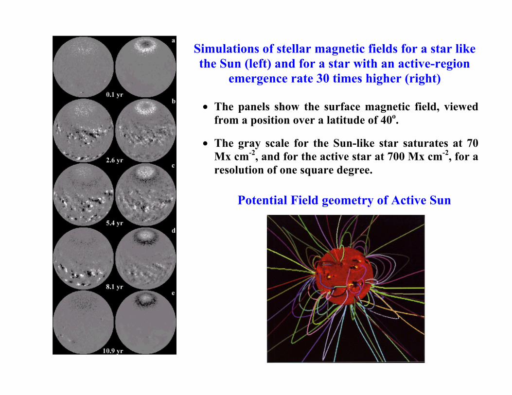
Simulations of stellar magnetic fields for a star like the Sun (left) and for a star with an active-region

emergence rate 30 times higher (right)

• The panels show the surface magnetic field, viewed from a position over a latitude of 40o.

• The gray scale for the Sun-like star saturates at 70 Mx cm-2, and for the active star at 700 Mx cm-2, for a resolution of one square degree.

Potential Field geometry of Active Sun

Potential field geometry of Stellar Coronae

• Each of the panels shows 500 randomly selected field lines (including in that total field lines behind the sphere).

• The columns show: a star of solar

activity, and stars with 10 and 30 times the solar active-region emergence rate, respectively.

• Six different phases of the 11-year

starspot cycles: 0.00 (top, cycle minimum), 0.16, 0.33, 0.49 (near cycle maximum), 0.65, and 0.82 (bottom). Sample magnetograms for these phases for the simulations of the Sun-like star and of the most active star are shown in Fig. above.

• The field line density within each

panel is statistically proportional to field strength.

Dynamic finely structured stellar atmosphere


Stellar magnetic activity => wealth of phenomena: starspots,nonradiatively heated outer atmospheres, activity cycles, decelera-tion of rotation rates, and even, in close binaries, stellar cannibalism.

Key topics : radiative transfer, convective simulations, dynamotheory, outer – atmospheric heating, stellar winds and angular mo-mentum loss.

Magnetically active stars shed angular momentum – losemass through their asterospheric magnetic fields. This process in-volves the interaction of a topologically complex, evolving coronalmagnetic field with embedded plasma, which is heated throughoutthe corona + accelerated on its way to interstellar space.

Stellar observations suggest: Sun was magnetically active evenbefore it became a hydrogen-burning star. Activity smoothlydeclining over billions of years – angular momentum is lost througha magnetized solar wind (e.g., Schrijver et al. 2003).

Evolution of corona cartoon: gravitationally stratified layers in the 1950s (left); vertical flux tubes with chromospheric canopies (1980s, middle); fully inhomogeneous mixing of photospheric, chromospheric, TR and coronal zones by such processes as heated upflows, cooling downflows, interminent heating (ε), nonthermal electron beams (e), field line motions and reconnections, emission from hot plasma, absorption and scattering in cool plasma, acoustic waves, shock waves (right) (Shrijver 2001).

Associating the traditional layers with temperature rather than height is only a little better.

The multi-temperature structure of the solar corona is visualized with images in different wavelengths. (Courtesy of Lockheed-Martin Solar and Astrophysics Lab.)

Plasma β in the solar atmosphere for two assumed field strengths, 100 G and 2500 G (Courtesy of G. Allen Gary)


Processes – Quiescent and ViolentQuiescent: Formation of long lived coronal structures, Heating, Mainte-

nance and Slow dissipation of these structures – solar winds (slow & fast),

acceleration, flow generation, waves, Surface turbulence, granulation etc.

Violent – explosive events like blinkers, sudden cell and network bright-

enings, flares, coronal mass ejection (CME’s).

Slow or fast, peaceful or violent – these processes represent conversion of

one form of energy into another. And there are really only three forms

of energy which play a fundamental role- magnetic, thermal and kinetic –

gravity also plays some some role but not a determining one.

Flares convert magnetic energy to heat and motion. CME’s destroy mag-

netic and heat for mass motion – both processes are catastrophic. The

latter takes plasma from the low corona into the SW and can disturb the

near–Earth space.

Each flux emergence brings helicity to accumulate additively in

a coronal structure while excess magnetic energy is flared away.

Catastrophic Events (Explosive/eruptive events like jet-like outflows, transient brightenings,

blinkers, large flares, nano- and micro-flares, eruptions, CME)

The dynamic, flaring, eruptive and explosive Solar Corona

TRACE: A set of coronal loops marked, of which five exhibit transverse oscillations

SOHO/LASCO images of a coronal mass ejection on 6 November 1997

A time sequence of Solar Maximum Mission coronagraph images showing a CME on August 18, 1980 (from Hundhausen (1999))

Eruption from Solar Surface

Sun and Earth

Coronal Mass Ejection

Coronal mass ejections (a) pre-eruption, (b and c) eruption, and (d) post-eruption states depicted by the mass-loading model, from Low (2001)

Field lines showing magnetic configurations in a numerical simulation, from Amari et al. (2003a)

Magnetic energy is built up by twisting foot points of initial bipolar potential field (a). After this building (b), twisting is stopped, field is allowed to relax to force-free equilibrium. Flux ropes may form (c) either by imposing further foot-point converging motions of the bipolar field or by imposing a slow diffusion of the normal field at the boundary. Eruption may occur: by flux cancellation at the boundary, by further imposing foot-point converging motions, or by imposing the diffusion of the boundary normal field beyond a certain threshold; the rising flux rope resembles a three-part CME (d).

Evolution of magnetic configurations for the slow (top panels) and fast (bottom panels)

coronal mass ejections cases (from Low & Zhang 2002). During the eruption, the dissipation of the current sheet (CS) produces foot-point brightenings (FB) in newly reconnected fields as the prominence (P) travels out with the ejected magnetic flux rope.

Quiescent events (Fast and slow SW, quasi-static loops, polar and transient CH-s, spicules)

Fine structure of Solar Atmosphere: Quiescent solar coronal loops over active regions - co-existed varying scale different temperature closed field structures (Aschwanden, Schrijver & Alexander (2000)).

Quasi-steady Solar Wind

Different dynamical behavior of constituting species


Corona - Observations - Inferences

• The solar corona – a highly dynamic arena replete withmulti-species multiple–scale spatiotemporal structures.

• Magnetic field was always known to be a controlling player.

• Enters a major new element – discovery that strong flows arefound everywhere in the low atmosphere — in the sub-coronal (chromosphere) as well as in coronal regions.

• Directed kinetic energy has to find its rightful place in dynam-ics: the plasma flows may, in fact, do complement theabilities of the magnetic field in the creation of theamazing richness observed in the coronal structures.

Challenge – to develop a theory of energy transformations for un-derstanding the quiescent and eruptive/explosive events.


How does the Solar Corona get to be so hot?

The temperature of the solar corona is a million K ( 100eV)(Grotrian 1939; Edlen 1942) – so much hotter than the photosphere(less than an eV for the Sun and other cool stars. How does it getto be so hot – still an unsolved problem!

Models galore – never a lack of suggestions – the problem is howto prove or disprove a model with the help of observations.Is it the ohmic or the viscous dissipation? or is it the shocks or thewaves that impart energy to the particles – And do the observationssupport the ”other consequences” of a given model?

– Recently developed notions that formation and heating of coronalstructures may be simultaneous and directed flows may be the car-riers of energy within a broad uniform physics framework opens anew channel for exploration.


The Solar Wind (SW) – History

Hydrodynamical expansion of the corona makes the wind.

Serious difficulty: the particles in fast component of the solar wind(FSW) have velocities considerably higher than the coronal protonthermal velocity (> 300 kms−1). Naturally such fast particles couldnot come from a simple pressure driven expansion.

Rescue: additional energy sources for accelerating the windto observed velocities. Birth of a new acceleration industry. Myr-iad mechanisms

Expansion/acceleration takes place in the regions called the coronalholes where the magnetic field influence can be neglected. But thewind comes from everywhere – How so? How do the charge particlesbeat the closed line magnetic fields?

Schematic illustration of the reconnection modelof a solar flare for the simplest bipole case. Thick solid lines show the magnetic field. Arrowsindicate the plasma bulk flow.

Reconnection – A digression

Sketch of a theoretical model that explains thethermal homogeneity of coronal loops for widthsof ≤≤≤≤ 2000 km, based on the magnetic field expan-sion from intergranular photospheric locations.

The heated plasma is uniformly spread over theentire loop cross section at a height where theplasma parameter exceeds the value of unity - inthe upper chromosphere / lower transition region.


A sample of modelsMagnetic reconnection and microflares =⇒ Generate fast shocks =⇒Protons and minor ions are heated and accelerated by fast shocks (lo-cal heating).

Microflares can be random in space and time =⇒ corona is heated.

Fast shocks generated by the magnetic reconnections with a smallerscale in chromosphere can produce Spicules.

Cascade of shock wave interactions in TR may lead to acceleration.Here are typical observational constraints on the theory:

• Acceleration must be completed very near the Solarsurface.

• Large anisotropy in the electron and proton temperatures – thereal mechanism must preferentially heat ions.


Present State of Art:

Energy transport and particle channeling mechanisms in the stellar atmo-

sphere are connected to the challenging problems of coronal heating and

stellar wind origin.

Neither the SW ”acceleration” nor the numerous eruptive events in the

stellar atmosphere can be treated as isolated and independent problems;

they must be solved simultaneously along with other phenomena like the

plasma heating (may take place in different stages). Any particular mech-

anism may be dominant in a specific region of parameter space.

For the solar wind there is another serious problem. What is the source of

matter and energy – the corona or the sub coronal regions (chromosphere,

photosphere, more directly from the sun).

Growing consensus: the same mechanism that transports mechanical

energy from convection zone to chromosphere to sustain its heating rate

also supplies the energy to heat corona and accelerate SW.


Towards a General Unifying Model:Need for a theory for general global dynamics that operates in a given

region of solar atmosphere.

In addition to the magnetic field, the plasma flows are also ac-

corded a place of honour. Both of these have origins in the

sub-atmospheric region and will jointly participate in the cre-

ation of a rich variety of coronal structures..

The magneto-fluid equations should cover both the open and the closed field regions. The difference

between various sub–units of the atmosphere will come from the initial and the boundary conditions.

Conjecture: the formation and primary heating of the coronal structures

as well as the more violent events (flares, erupting prominences and CMEs)

are the expressions of different aspects of the same general global dynamics

that operates in a given coronal region.

The plasma flows, the source of both the particles and energy (part of

which is converted to heat), interacting with the magnetic field, become

dynamic determinants of a wide variety of plasma states =⇒ the immense

diversity of the observed coronal structures.


Magneto-fluid Coupling

V — the flow velocity field of the plasmaTotal current j = j0 + js. js – self-current (generates Bs).Total (observed) magnetic field — B = B0 + Bs.

The stellar atmosphere is finely structured.Multi-species, multi-scales. Simplest – two-fluid approach.Quasineutrality condition: ne ' ni = nThe kinetic pressure: p = pi + pe ' 2 nT, T = Ti ' Te.

Electron and proton flow velocities are different.

Vi = V, Ve = (V − j/en)

Nondissipative limit: electrons frozen in electron fluid; ion fluid (finite inertia) moves distinctly.

Heating due to the viscous dissipation of the flow vorticity:[

d

dt

(miV2

2

)]

visc

= −minνi

(12(∇×V)2 +

23(∇ ·V)2

). (1)


Normalizations:n → n0 – the density at some appropriate distance from surface,B → B0 – the ambient field strength at the same distance|V | → VA0 – Alfven speed

Parameters:rA0 = GM/V 2

A0R0 = 2β0 rc0, α0 = λi0/R0, β0 = c2s0/V 2

A0,cs0 — sound speed R0 — the characteristic scale length,λi0 = c/ωi0 — the collisionless ion skin depthare defined with n0, T0, B0.

Hall current contributions are significant whenα0 > η, (η - inverse Lundquist number).Important in: interstellar medium, turbulence in the early uni-verse, white dwarfs, neutron stars, stellar atmosphere.Typical solar plasma: condition is easily satisfied.


Construction of a Typical Coronal structure

Solar Corona — Tc = (1÷ 4) · 106 K nc ≤ 1010 cm−3.Standard picture – Corona is first formed and then heated.3 principal heating mechanisms:

• By Alfven Waves,• By Magnetic reconnection in current sheets,• MHD Turbulence.

All of these attempts fall short of providing a continuous energy sup-ply that is required to support the observed coronal structures.

New concept: Formation and heating are contempraneous – the primary

flows are trapped and a part of their kinetic energy dissipates during their

trapping period. It is the Initial and boundary conditions that define the

characteristics of a given structure . Tc À T0f 1eV .

Observations −→ there are strongly separated scales both in time and

space in the solar atmosphere. And that is good.


A coronal structure – 2 distinct eras:

1. A hectic dynamic period when it acquires particles and energy (ac-

cumulation + primary heating) – Full description needed: time

dependent dissipative two-fluid equations are used. Heating takes

place while particles accumulate (get trapped) in a curved magnetic field.

Simulations show that kinetic energy contained in the primary

flows can be dissipated by viscosity, and that this dissipation

can be large enough to provide the continuous heating up to

observed temperatures.

2. Quasistationary period when it ”shines” as a bright, high tempera-

ture object — a reduced equilibrium description suffices; collisional effects

and time dependence are ignored.

Equilibrium: each coronal structure has a nearly constant T , but differ-

ent structures have different characteristic T -s, i.e., bright corona seen as

a single entity will have considerable T–variation.


1st Era – Fast dynamicEnergy losses from corona F ∼ (5 · 105 ÷ 5 · 106) erg/cm2

s.If the conversion of the kinetic energy in the PF-s were to compensatefor these losses, we would require a radial energy flux

12min0V

20 V0 ≥ F,

For initial V0 ∼ (100÷900) km/s n ∼ 9·105÷107 cm−3 – viscousdissipation of the flow takes place on a time:

tvisc ∼ L2

νi, (2)

For flow with T0 = 3 eV = 3.5 · 104 K, n0 = 4 · 108 cm−3 creatinga quiet coronal structure of size L = (2 · 108 ÷ 1010) cm, tvisc ∼(3.5 · 108 ÷ 1010) s.Note: (2) is an overestimate. treal ¿ tvisc.Reasons: 1) νi = νi(t, r) will vary along the structure,2) the spatial gradients of the V–field can be on a scale much shorterthan L (defined by the smooth part of B–field).

-0.4 -0.2 0.0 0.2 0.4

x

0.10.20.30.40.50.6

z

-0.8 -0.4 0.0 0.4 0.8x

0.00E+0

1.00E+7

2.00E+7

3.00E+7

Vz(x)

Contour plots for the vector potentialA (flux function) in the x – z plane fora typical arcade-like solar magneticfield.

The distribution of the radialcomponent Vz (with a maximum of 300 km/s at t=0) for the symmetric,spatially nonuniform velocity field.

t = 43s n/n0 T[eV] |V| [cm/s]

-0.4 -0.2 0.0 0.2 0.4x

0.10.20.30.40.5

z

1.0

2.0

3.0

4.0

5.0

6.0

-0.4 -0.2 0.0 0.2 0.4

x

0.10.20.30.40.5

26101418222630

-0.4 -0.2 0.0 0.2 0.4

x

0.10.20.30.40.5

0.0E+0004.0E+0068.0E+0061.2E+0071.6E+0072.0E+0072.4E+0072.8E+007

t = 181 s

-0.4 -0.2 0.0 0.2 0.4x

0.10.20.30.40.5

z

1.02.54.05.57.08.510.011.5

-0.4 -0.2 0.0 0.2 0.4

x

0.10.20.30.40.5

0102030405060708090

-0.4 -0.2 0.0 0.2 0.4

x

0.10.20.30.40.5

0.0E+000

6.0E+006

1.2E+007

1.8E+007

2.4E+007

3.0E+007

t = 376 s

-0.4 -0.2 0.0 0.2 0.4x

0.10.20.30.40.5

z

1.03.05.07.09.011.013.015.0

-0.4 -0.2 0.0 0.2 0.4

x

0.10.20.30.40.5

020406080100120140

-0.4 -0.2 0.0 0.2 0.4

x

0.10.20.30.40.5

0.0E+0002.0E+0064.0E+0066.0E+0068.0E+0061.0E+0071.2E+0071.4E+007

Hot coronal structure formation. Initial parameters: the flow T0 =3 eV and n0 =4••••108 cm-3 , the initial background density =2••••108 cm-3 , Bmax (x0 , z0=0)=20 G. The primary heating is completed in ~(2 – 3) min on distances ~10 000 km. The heating is symmetric and the resulting hot structure is heated to 1.6••••106 K. Much of the primary flow kinetic energy has been converted to heat via shock generation.

t = 91s n/n0 T[eV] |V| [cm/s]

-0.4 -0.2 0.0 0.2 0.4

x

0.10.20.30.40.50.6

z

1.02.03.04.05.06.07.0

-0.4 -0.2 0.0 0.2 0.4

x

0.10.20.30.40.50.6

0

8

16

24

32

40

-0.4 -0.2 0.0 0.2 0.4

x

0.10.20.30.40.50.6

0.0E+000

6.0E+006

1.2E+007

1.8E+007

2.4E+007

3.0E+007

t = 201s

-0.4 -0.2 0.0 0.2 0.4

x

0.10.20.30.40.50.6

z

1.0

2.0

3.0

4.0

5.0

6.0

-0.4 -0.2 0.0 0.2 0.4

x

0.10.20.30.40.50.6

0

10

20

30

40

50

-0.4 -0.2 0.0 0.2 0.4

x

0.10.20.30.40.50.6

0.0E+000

6.0E+006

1.2E+007

1.8E+007

2.4E+007

3.0E+007

t = 472s

-0.4 -0.2 0.0 0.2 0.4

x

0.10.20.30.40.50.6

z

1.02.03.04.05.06.07.08.0

-0.4 -0.2 0.0 0.2 0.4

x

0.10.20.30.40.50.6

0102030405060

-0.4 -0.2 0.0 0.2 0.4

x

0.10.20.30.40.50.6

0.0E+000

6.0E+006

1.2E+007

1.8E+007

2.4E+007

3.0E+007

Hot Coronal Structure Creation

The interaction of an initially asymmetric, spatially nonuniform primary flow (just the right pulse) with a strong arcade-like magnetic field Bmax (x0 , z0=0)=20 G.

Downflows, and the imbalance in primary heating are revealed


2nd Era – Quasi Equilibrium

• The familiar magneto hydrodynamics (MHD) theory (singlefluid) is inadequate – The fundamental contributions of thevelocity field do not come through.

• Equilibrium states (relaxed minimum energy states) encoun-tered in MHD do not have enough structural richness.

In a two-fluid description, the velocity field interacting with the mag-netic field provides:

• new pressure confining states

• the possibility of heating these equilibrium states by dissipa-tion of short scale kinetic energy.

Let us now construct a simple equilibrium theory.


A Quasi-equilibrium Structure

Model: recently developed magnetofluid theory.

Assumption: at some distance there exist fully ionized and magne-tized plasma structures such that the quasi–equilibrium two–fluidmodel will capture the essential physics of the system.

Simplest two–fluid equilibria: T = const −→ n−1∇p → T∇ ln n.Generalization to homentropic fluid: p = const·nγ is straightforward.The dimensionless equations:

1n∇× b× b +∇

(rA0

r− β0 ln n− V 2

2

)+ V × (∇×V) = 0, (3)

∇×[(

V − α0

n∇× b

)× b

]= 0, (4)

∇ · (nV) = 0, (5)∇ · b = 0, (6)


The system allows the following relaxed state solution

b + α0∇×V = d n V, b = a n[V − α0

n∇× b

], (7)

augmented by the Bernoulli Condition

∇(

2β0rc0

r− β0 ln n− V 2

2

)= 0 (8)

a and d — dimensionless constants related to ideal invari-ants: The Magnetic and the Generalized helicities

h1 =∫

(A · b) d3x, (9)

h2 =∫

(A + V) · (b +∇×V)d3x.. (10)

The system is obtained by minimizing the energy E =∫

(b ·b + nV ·V) d3x keeping h1 and h2 invariant.


Equations (7) yield

α20

n∇×∇×V + α0 ∇×

(1a− d n

)V +

(1− d

a

)V = 0. (11)

which must be solved with (8) for n and V.Equation (8) is solved to obtain (g(r) = rc0/r)

n = exp(−

[2g0 − V 2

0

2β0(T )− 2g +

V 2

2β0(T )

]), (12)

The variation in density can be quite large for a low β0 plasma if the gravity and the flow kinetic

energy vary on length scales comparable to the extent of the structure.

Model calculation – temperature varying but density constant (n =1); The following still holds (where Q is either V or b):

α20 ∇×∇×Q + α0

(1a− d

)∇×Q +

(1− d

a

)Q = 0 (13)


Curl Curl Equation – Double-Beltrami states

With p = (1/a− d) and q = (1− d/a), Eq. (13) =⇒(α0∇×−λ)(α0∇×−µ)b = 0 (14)

where λ(λ+) and µ(λ−) are the solutions of the quadratic equation

α0λ± = −p

2±

√p2

4− q. (15)

If Gλ is the solution of the Beltrami Equation (aλ and aµ are con-stants)

∇×G(λ) = λG(λ), then (16)

b = aλG(λ) + aµG(µ), (17)

is the general solution of the double curl equation. Velocity field is:

V =ba

+ α0∇∇∇× b =(

1a

+ α0λ

)aλG(λ) +

(1a

+ α0µ

)aµG(µ).

(18)Double curl equation is fully solved in terms of the solutions of Eq. (21).


Double Beltrami States

• There are two scales in equilibrium unlike the standard case.

• A possible clue for answering the extremely important question:

why do the coronal structures have a variety of length scales, and

what are the determinants of these scales?

• The scales could be vastly separated – are determined by the con-

stants of the motion – the original preparation of the system. These

constants also determine the relative kinetic & magnetic energy in quasi-equilibrium.

• The scales could be a complex conjugate pair – the fields will be obtained

by an appropriate real combination – change in the topological character of

the flow and magnetic fields.• The short scale is a result of a singular perturbation on the standard

MHD system – introduces classes of states inaccessible to MHD.

• It is all a consequence of treating flows and magnetic field co-equally.

• These vastly richer structures can and do model the quiescent solar

phenomena rather well – construction of coronal arcades fields, slow

acceleration, spatial rearrangement of energy etc.


An Example of structural richness

In a coronal structure, the magnetic field is relatively smooth but the ve-

locity field must have a considerable short – scale component if its dissipa-

tion were to heat the plasma. Can a Double Beltrami state provide that?

Sub–Alfvenic Flow: a ∼ d À 1 =⇒ λ ∼ (d− a)/α0 d a, µ = d/α0.

V =1

aaλGλ + daµG(µ) (19)

b = aλGλ + aµG(µ) (20)

while, the slowly varying component of velocity is smaller by a factor

(a−1 ' d−1) compared to similar part of b-field, the fast varying compo-

nent is a factor of d larger than the fast varying component of b-field!

Result: for an extreme sub–Alfvenic flow (e.g. |V| ∼ d−1 ∼ 0.1),

|V(µ)||V(λ)| ' 1; (21)

the velocity field is equally divided between slow and fast scales.


Acceleration of Plasma Flows

The most obvious process for acceleration (rotation is ignored):

• the conversion of magnetic• and/or the thermal energy

to plasma kinetic energy.

Magnetically driven transient but sudden flow–generation models:• Catastrophic models• Magnetic reconnection models• Models based on instabilities

Quiescent pathway:• Bernoulli mechanism converting thermal energy into kinetic• General magnetofluid rearrangement of a relatively constant

kinetic energy: going from an initial high density–low velocityto a low density–high velocity state.


Eruptive and Explosive events, FlaringWhat happens when the parameters of the DB field change? Assume

• The parameter change is sufficiently slow / adiabatic.

• At each stage, the system can find its local DB equilibrium.

• In slow evolution the dynamical invariants: h1, h2, and the total

(magnetic plus the fluid) energy E are conserved.

Can such a slowly evolving structure suffer a catastrophic loss

of equilibrium? The General equilibrium solution was shown to be

b = CµGµ(µ) + CλGλ(λ), (22)

V =(

1

a+ µ

)CµGµ(µ) + Cλ

(1

a+ λ

)Gλ(λ). (23)

The transition may occur in one of the following two ways:

1. When the roots (λ - large-scale, µ - short-scale) of the quadratic

equation, determining the length scales for the field variation, go

from being real to complex.

2. Amplitude of either of the 2 states (Cµ/ν) ceases to be real.


The three invariants h1, h2 and E (quantum nmbers) provide three rela-

tions connecting 4 parameters λ, µ, Cλ, Cµ that characterize the DB field.

Large scale λ – control parameter — observationally motivated choice.

Study the structure–structure interactions working with simple 2DBeltrami ABC field with periodic boundary conditions.

Choose real λ, µ for quasi–equilibrium structures in atmospheres.

There are two scenarios of losing equiliubrium:(1) Either of (Cµ/ν)2 becomes zero (starting from positive values) forreal λµ/ν ,(2) The roots λµ/ν coalesce (λµ ↔ λν) for real λµ/ν and Cµ/ν .

Solar atmosphere: equilibria with vastly separated scales (for a va-riety of sub–alfvenic flows). (2) possibility is not of much relevance.

Flow Acceleration (n=const)

2D Beltrami ABS Field with periodic boundary conditions

a) No catastrophe initial conditions

b) Catastrophe initial conditions

a) No catastrophe initial conditions b) Catastrophe initial conditions

Solar Atmosphere: Almost all initial magnetic energy (short scale) is transferred to flow

Root coalescence: No separation between roots at the transition!


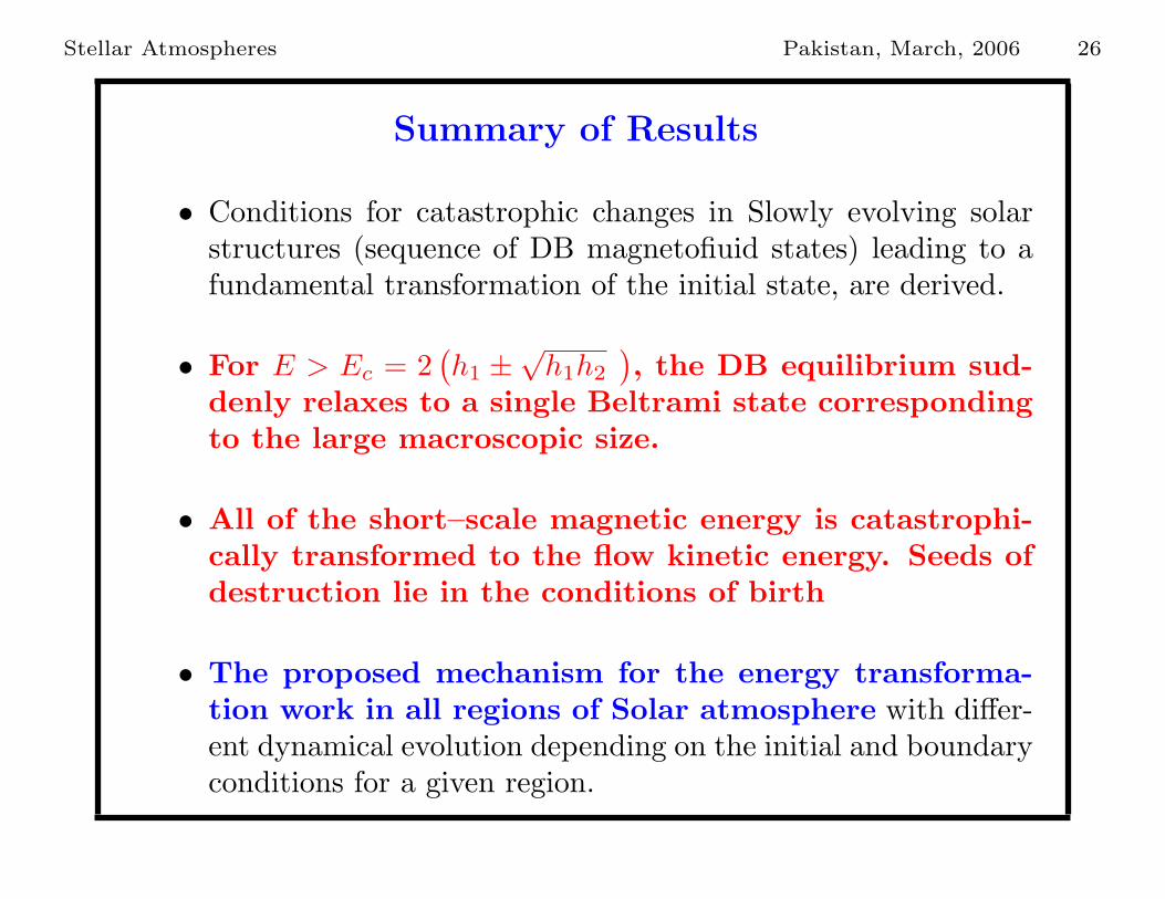
Summary of Results

• Conditions for catastrophic changes in Slowly evolving solarstructures (sequence of DB magnetofiuid states) leading to afundamental transformation of the initial state, are derived.

• For E > Ec = 2(h1 ±

√h1h2

), the DB equilibrium sud-

denly relaxes to a single Beltrami state correspondingto the large macroscopic size.

• All of the short–scale magnetic energy is catastrophi-cally transformed to the flow kinetic energy. Seeds ofdestruction lie in the conditions of birth

• The proposed mechanism for the energy transforma-tion work in all regions of Solar atmosphere with differ-ent dynamical evolution depending on the initial and boundaryconditions for a given region.


Non–uniform density case

Variational Principle =⇒ One can deal with any case:constant density, constant temperature, or a given equation of state.

Closed system (3), (7),(8) with g(r) = rc0/r =⇒α2

0

n∇×∇×V + α0 ∇×

[(1

an− d

)nV

]+

(1− d

a

)V = 0, (24)

α20∇×

(1n∇× b

)+α0 ∇×

[(1

an− d

)b]+

(1− d

a

)b = 0. (25)

n = exp(−

[2g0 − V 2

0

2β0− 2g +

V 2

2β0

]), (26)

Caution: this time–independent set is not suitable for studyingprimary heating processes at lower heights (Mahajan et al. PoP 2001).

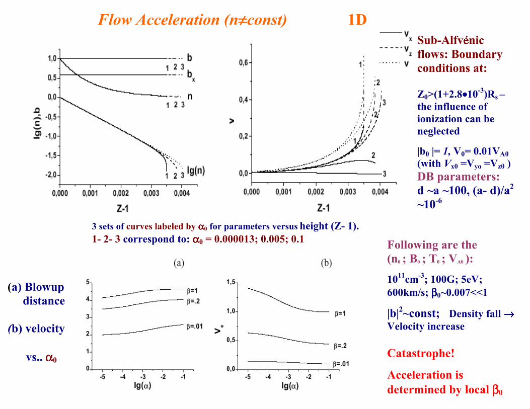
3 sets of curves labeled by αααα0 for parameters versus height (Z- 1). 1- 2- 3 correspond to: αααα0 = 0.000013; 0.005; 0.1

Sub-AlfvJJJJnic flows: Boundary conditions at: Z0>(1+2.8••••10-3)Rs – the influence of ionization can be neglected

|b0 |= 1, V0= 0.01VA0 (with Vx0 =Vyo =Vz0 ) DB parameters: d ~a ~100, (a- d)/a2 ~10-6

Following are the (n0 ; B0 ; T0 ; VA0 ):

1011cm-3; 100G; 5eV; 600km/s; ββββ0~0.007<<1

|b|2~const; Density fall →→→→ Velocity increase Catastrophe!

Acceleration is determined by local ββββ0

Flow Acceleration (n≠≠≠≠const) 1D

(a) Blowup distance (b) velocity vs.. αααα0


Where do the flows come from?

The Dynamo mechanism is the generic process of generating macroscopic

magnetic fields from an initially turbulent system. It is biggest industry

in plasma astrophysics; is highly investigated in a variety of fusion devices.

Standard Dynamo – generation of macroscopic fields from (primarily

microscopic) velocity fields. The relaxations observed in the reverse field

pinches is a vivid illustration of the Dynamo in action. The Myriad phe-

nomena in stellar atmospheres (heating, field opening, wind) impossible

to explain without knowing the origin/nature of magnetic field structures.

In the so called kinematic dynamo, the velocity field is externally

specified and is not a dynamical variable. In ”higher” theories

– MHD, Hall MHD, two fluid etc, the velocity field evolves just

as the mag. field does – the fields are in mutual interaction.

Short-scale turbulence → macroscopic magnetic fields. Will turbulence,

under appropriate conditions => macroscopic plasma flows?


Reverse Dynamo – Flow generationIf the process of conversion of short–scale kinetic energy to long–scalemagnetic energy is termed ”dynamo” (D) then the mirror image pro-cess of the conversion of short–scale magnetic energy to long–scalekinetic energy could be called ”Reverse dynamo” (RD).

Extending the definitions:• Dynamo(D) process - Generation of macroscopic magnetic

field from any mix of short–scale energy (magnetic and kinetic).

• Reverse Dynamo(RD) process - Generation of macroscopicflow from any mix of short–scale energy (magnetic and kinetic).

Theory and simulation show(1) D and RD processes operate simultaneously — whenever a largescale magnetic field is generated there is a concomitant generationof a long scale plasma flow.(2) The composition of the turbulent energy determines the ratio ofthe macroscopic flow/macroscopic magnetic field.


Reverse Dynamo relationship — Theory

Minimal two fluid model – incompressible, constant density HMHD-gravity is ignored

∂B

∂t= ∇×

[[V −∇×B]×B

], V e = V −∇×B(27)

∂V

∂t= V × (∇× V ) + (∇×B)×B −∇

(P +

V 2

2

)(28)

The total fields are broken into ambient fields and perturbationsB = b0 + H + b

V = v0 + U + v

b0, v0 - equilibrium; H, U - macroscopic; b, v - microscopic fields.Equilibrium fields are taken to be the DB pairobeying Bernoulli condition ∇(p0 + v0

2/2) = const

b0

a+ ∇× b0 = v0, b0 + ∇× v0 = dv0, (29)


which may be solved in terms of the SB fields (∇×G(µ) = µG(µ))Inverse scale lengths λ, µ are fully determined in terms of a, d (hence, initial helicities). As a, d

vary, λ, µ can range from real to complex values of arbitrary magnitude.

Below: λ - micro-scale; µ - macro-scale structures; |b| ¿ b0, |v| < v0 at the same scale;

ve0 ≡ v0 −∇ × b0.See for the details of closure model of Hall MHD Mininni et al, ApJ, 2003, 2005.

Evolution Equations of the macrofields:

∂tU = U × (∇×U) + ∇×H ×H + 〈v0 × (∇× v)〉+ 〈v × (∇× v0) + (∇× b0)× b + (∇× b)× b0〉

− 〈∇(v0 · v)〉 −∇(

p +U2

2

)(30)

∂H

∂t= ∇× 〈[ve × b0] + ve0 × b〉+ ∇× [(U −∇×H)×H] (31)

where the blue terms are nonlinear and the ensemble averages of theblack terms have to be found after solving for v and b.


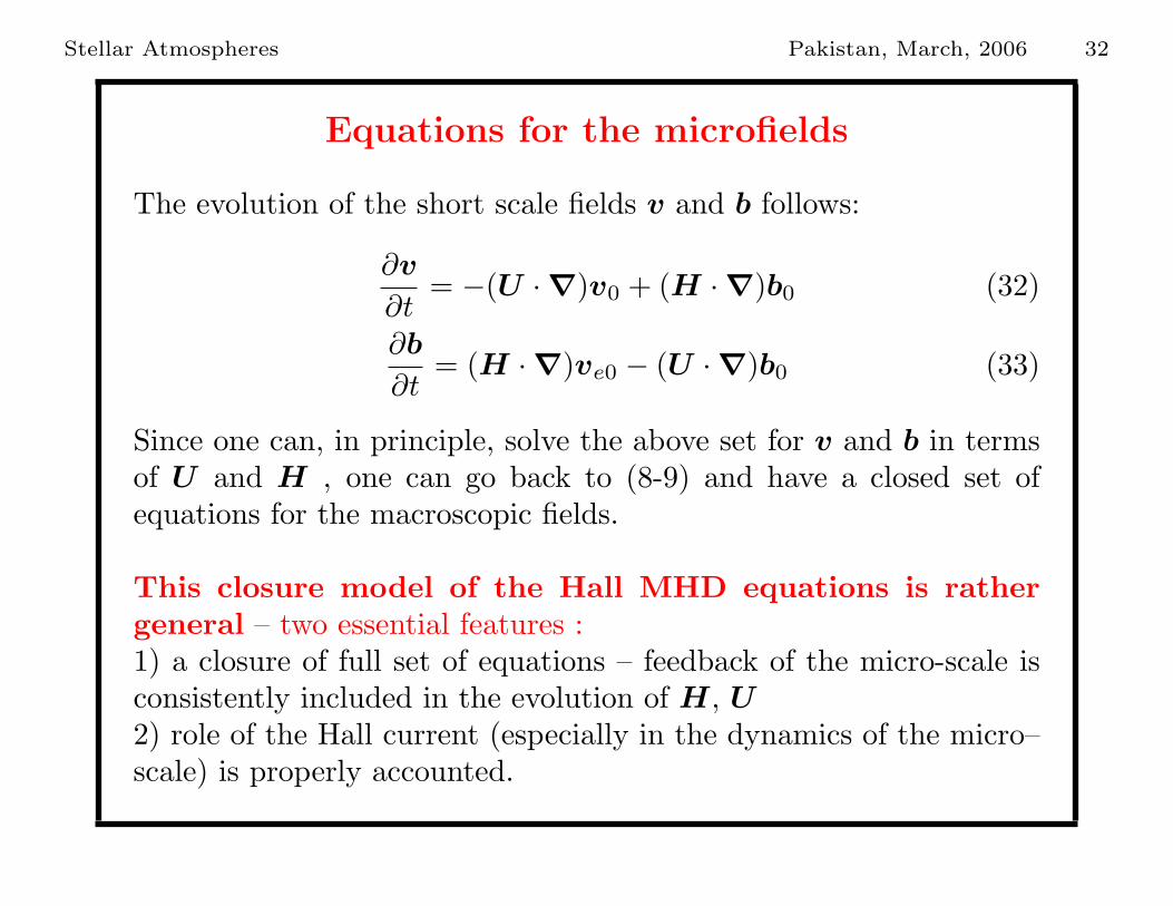
Equations for the microfields

The evolution of the short scale fields v and b follows:

∂v

∂t= −(U ·∇)v0 + (H ·∇)b0 (32)

∂b

∂t= (H ·∇)ve0 − (U ·∇)b0 (33)

Since one can, in principle, solve the above set for v and b in termsof U and H , one can go back to (8-9) and have a closed set ofequations for the macroscopic fields.

This closure model of the Hall MHD equations is rathergeneral – two essential features :1) a closure of full set of equations – feedback of the micro-scale isconsistently included in the evolution of H, U2) role of the Hall current (especially in the dynamics of the micro–scale) is properly accounted.


Short Scale Initial Fields

The model calculation is best done by assuming that the originalequilibrium is predominantly short-scale. Thus from the DB fieldswe keep only the λ part. Following relations, then, follow:

v0 = b0

(λ + a−1

)(34)

leading tove0 = v0 −∇× b0 = b0 a−1 (35)

yielding the system:b =

(a−1H −U

) ·∇b0 (36)

v =(H − (

λ + a−1)U

) ·∇b0. (37)

Carrying out appropriate averages over the short scale ambient fields(all expressed in terms b0) will give us the time behavior of the macrofields U and H.

Spatial averages with isotropic ABC flow yield:


U = bN1 +λ

2b20

3∇×

[((λ +

1a

)2)

U − λH

](38)

H = bN2 − λb20

3

(1− λ

a− 1

a2

)∇×H. (39)

where N1 and N2 are the time derivatives of the nonlinear terms displayed earlier - they will not

change on short-scale averaging. b20 measures the ambient micro scale energy.

H evolves independently of U but evolution of U does require knowledge of H.

Neglecting the nonlinear terms and writing (52),(53) formally as

H = −r(λ)(∇×H), U = ∇× [s(λ)U + q(λ)H], (40)

Fourier analyzing we find the growth rate at which H, U increase,

ω4 = r2k2 ω2 = −|r|(k). (41)The growing Macro-fields are related as

U =q

(s + r)H. (42)


A Nonlinear Solution in Linear Clothing

The linear solution has a few remarkable features:

Since a choice of a, d (and hence of λ) fixes relative amountsof microscopic energy in ambient fields, it also fixes the relativeamount of energy in the nascent macroscopic fields U and H.

The linear solution makes nonlinear terms strictly zero – itis an exact (a special class) solution of the nonlinear systemand thus remains valid even as U and H grow to larger am-plitudes.

(This behavior appears again and again in Alfvenic systems: MHD- nonlinear Alfven wave: Walen 1944,1945; in HMHD - Mahajan &Krishan, MNRAS 2005).


Analytical Results — An Almost straight dynamo

Explicit connections for mix in the ambient turbulence to the mix inthe macro fields.:(i) a ∼ d À 1 , inverse micro scale λ ∼ a À 1 =⇒ v0 ∼ a b0 À b0

, i.e, the ambient micro-scales fields are primarily kinetic. The Gen-erated macro-fields have opposite ordering, U ∼ a−1H ¿ H.

An example of the straight dynamo mechanism – super-Alfvenic”turbulent flows” generate magnetic energy far in excess of kineticenergy – super-Alfvenic ”turbulent flows” lead to steady flows thatare equally sub–Alfvenic.

Important: the dynamo effect must always be accompanied by thegeneration of macro-scale plasma flows.

This realization can have serious consequences for defining the initial setup for the later dynamics

in the stellar atmosphere. The presence of an initial macro-scale velocity field during the flux

emergence processes is, for instance, always guaranteed by the mechanism exposed above.


Analytical Results — An Almost Reverse dynamo

(ii) a ∼ d ¿ 1 the inverse micro scale λ ∼ a − a−1 À 1 =⇒v0 ∼ a b0 ¿ b0. The ambient energy is mostly magnetic. (Pho-tospheres/chromospheres)

Micro-scale magnetically dominant initial system creates macro-scalefields U ∼ a−1H À H that are kinetically abundant.

From a strongly sub-Alfvenic turbulent flow, the system generates astrongly super-Alfvenic macro–scale flow [reverse dynamo].

Initial Dominance of fluctuating/turbulent magnetic field + magneto-fluid coupling = efficient/significant acceleration. Part of the mag-netic energy will be transferred to steady plasma flows – a steadysuper–Alfvenic flow; a macro flow accompanied by a weak magneticfield.RD → observations: fast flows are found in weak field regions(Woo et al, ApJ, 2004).


D, RD Summary:

• Dynamo and ”Reverse Dynamo” mechanisms have the sameorigin – are manifestation of the magneto-fluid coupling;

• U and H are generated simultaneously and proportionately.Greater the macro-scale magnetic field (generated locally), greater the macro-scale velocity

field (generated locally);

• Growth rate of macro-fields is defined by DB parameters(by the ambient magnetic and generalized helicities) and scalesdirectly with ambient turbulent energy ∼ b2

0 (v20).

Larger the initial turbulent magnetic energy, the stronger the acceleration of the flow.

Impacts: on the evolution of large-scale magnetic fields andtheir opening up with respect to fast particle escape from stel-lar coronae; on the dynamical and continuous kinetic energysupply of plasma flows observed in astrophysical systems.Initial and final states have finite heliciies (magnetic and kinetic). The helicity densities

are dynamical parameters that evolve self-consistently during the flow acceleration.


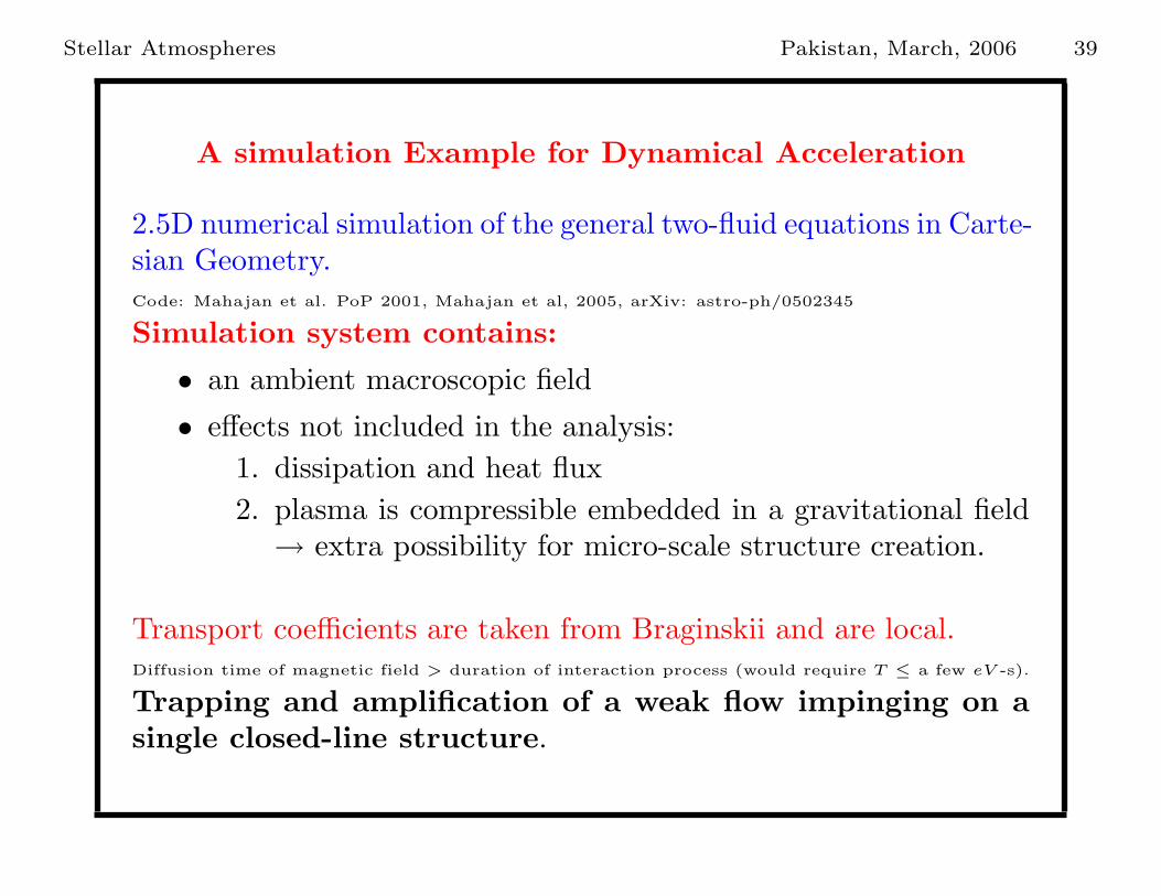
A simulation Example for Dynamical Acceleration

2.5D numerical simulation of the general two-fluid equations in Carte-sian Geometry.Code: Mahajan et al. PoP 2001, Mahajan et al, 2005, arXiv: astro-ph/0502345

Simulation system contains:

• an ambient macroscopic field

• effects not included in the analysis:1. dissipation and heat flux2. plasma is compressible embedded in a gravitational field→ extra possibility for micro-scale structure creation.

Transport coefficients are taken from Braginskii and are local.Diffusion time of magnetic field > duration of interaction process (would require T ≤ a few eV -s).

Trapping and amplification of a weak flow impinging on asingle closed-line structure.

Initial characteristics of magnetic field and flow

-0.6 -0.3 0.0 0.3 0.60.0

0.2

0.4

0.6

0.8

1.0 Ay

X

Z

-5E-3-6.3E-43.7E-38.1E-31.2E-21.7E-22.1E-22.6E-23E-2

0 50 100 150

0.000

0.005

0.010Vmax(t)/ VA

t-0.6 -0.3 0.0 0.3 0.6

0

1x105

2x105 -1

-

-0

n 0(t,x

,z=0

) [c

m-3]

V 0z(t,

x,z=

0) [

cm/s

]

x

zAB ˆBz+×∇= A(0; Ay; 0); b=B/B0z; bx(t, x, z ≠ 0) ≠ 0 B0z=100G - uniform it time. Weak symmetric up-flow (pulse-like): |V|0max<< Cs0 Cs0 - initial sound speed; time duration - t0=100s Initially Gaussian; peak is located in the central region of a single closed magnetic field structure. Initial flow parameters: V0max(x_o, z=0)=V0z=2.18•105cm/s; n0max=1012cm-3; T(x,z=0)=const=T0 =10,eV

Acceleration of plasma flow due to Magneto-fluid coupling - RD

• Acceleration is significant in the vicinity of magnetic field-maximum with strong deformation

of field lines + energy re-distribution due to MFC+dissipation

• A part of flow is trapped in the maximum field localization area, accumulated, cooled and accelerated. The accelerated flow reaches speeds greater than 100km/s in less than 100s

• Accelerated flow follows to the maximum magnetic field localization areas - RD

Then the flow passes through a series of quasi-equilibria. In this relatively extended era ~1000s of stochastic/oscillating acceleration, the intermittent flows continuously acquire energy → bifurcation Flow starts to accelerate again - acceleration highest in strong field regions (newly generated!)

Initial stage of acceleration: macroscopic magnetic energy → macroscopic flow energy Second stage of acceleration after the quasi-equilibrium: microscopic magnetic energy is converted to macroscopic flow energy


Simulation Summary:

• Dissipation present: Hall term (∼ α0) (through the mediation of micro-

scale physics) plays a crucial role in acceleration/heating processes

• Initial fast acceleration in the region of maximum original mag-netic field + the creation of new areas of macro-scale magneticfield localization with simultaneous transfer of the micro-scalemagnetic energy to flow kinetic energy = manifestations of thecombined effects of the D and RD phenomena

• Continuous energy supply from fluctuations (dissipative, Hall, vortic-

ity) → maintenance of quasi-steady flows for significant period

• Simulation: actual h1, h2 are dynamical. Even if they arenot in the required range initially, their evolution could bringthem in the range where they could satisfy conditions needed toefficiently generate flows → several phases of acceleration


Summing up:

• A two fluid theory in which the velocity field is treated at parwith the magnetic field has the potentials of creating an excel-lent theory for the structures present and phenomena observedin the solar atmosphere.

• Quasi-steady, fast, and even catastrophic phenomena have anunderlying unified description.

• Simple analysis can capture essential and qualitative aspects ofboth the quiescent and the violent processes. A violent fate ofa given structure is underwritten right at its moment of birth.

• Simulations are needed to capture what actually happens nearthe catastrophe.

Documents

Quiescent and Catastrophic Events In Stellar … and Catastrophic Events In Stellar Atmospheres Swadesh M. Mahajan ... Magnetic energy is built up by twisting foot points of initial