Quasi-Newton Methods for the Acceleration of Multi … · Quasi-Newton Methods for the Acceleration of Multi-Physics Codes Rob Haelterman, Alfred Bogaers, Joris Degroote, Nicolas

Quasi-Newton Methods for the Acceleration ofMulti-Physics Codes

Rob Haelterman, Alfred Bogaers, Joris Degroote, Nicolas Boutet

Abstract—Often in nature different physical systems interactwhich translates to coupled mathematical models. Even if pow-erful solvers often already exist for problems in a single physicaldomain (e.g. structural or fluid problems), the development ofsimilar tools for multi-physics problems is still ongoing. Whenthe interaction (or coupling) between the two systems is strong,many methods still fail or are computationally very expensive.Approaches for solving these multi-physics problems can bebroadly put in two categories: monolithic or partitioned. Whilewe are not claiming that the partitioned approach is panaceafor all coupled problems, here we will only focus our attentionon studying methods to solve (strongly) coupled problems witha partitioned approach in which each of the physical problemsis solved with a specialized code that we consider to be a blackbox solver and of which the Jacobian is unknown. We alsoassume that calling these black boxes is the most expensivepart of any algorithm, so that performance is judged by thenumber of times these are called.Running these black boxes one after another, until convergenceis reached, is a standard solution technique and can beconsidered as a non-linear Gauss-Seidel iteration. It is easyto implement but comes at the cost of slow or even conditionalconvergence. A recent interpretation of this approach as a root-finding problem has opened the door to acceleration techniquesbased on quasi-Newton methods. These quasi-Newton methodscan easily be “strapped onto” the original iteration loop withoutthe need to modify the underlying code and with little extracomputational cost.In this paper, we analyze the performance of ten accelerationtechniques that can be applied to accelerate the convergence ofa non-linear Gauss-Seidel iteration, on different multi-physicsproblems.

Index Terms—Partitioned methods, iterative methods, quasi-Newton.

I. INTRODUCTION

OFTEN in nature different systems interact, like fluidsand structures, heat and electricity, populations of

species, etc.Mathematically these can be written as the non-linear system

Manuscript received August 03, 2017.R. Haelterman is associate professor at the Royal Military Academy,

Dept. Mathematics, Renaissancelaan 30, B-1000 Brussels, Belgium. email:[email protected]

A. Bogaers is senior researcher at the Council for Scientific and Indus-trial Research, Advanced Mathematical Modelling, Modelling and DigitalSciences, Meiring Naude Road; Brummeria, Pretoria, South Africa and avisiting lecturer at the School of Computer Science and Applied Math-ematics, University of Witwatersrand, Johannesburg, South Africa. email:[email protected]

J. Degroote is associate professor at Ghent University, Dept. Flow,Heat and Combustion Mechanics, Sint-Pietersnieuwstraat 41, 9000 Ghent,Belgium. email: [email protected]

N. Boutet is PhD student at Ghent University, Dept. Flow, Heat andCombustion Mechanics, Sint-Pietersnieuwstraat 41, 9000 Ghent, Belgiumand Royal Military Academy, Dept. Mathematics, Renaissancelaan 30, B-1000 Brussels, Belgium. email: [email protected]

of equations given by

f1(x1, x2, . . . , xn) = 0f2(x1, x2, . . . , xn) = 0

...fn(x1, x2, . . . , xn) = 0

(1)

where fi : DF ⊂ Rm → Rki and xj ∈ Rmj (i, j ∈{1, 2, . . . , n}),

∑ni=1 ki = m,

∑nj=1mj = m.

Each equation describes (the discretized equations of)a physical problem that is spatially or mathematicallydecomposed. E.g. f1(x1, x2) = 0 could give the pressurex1 on the wall of a flexible tube for a given geometry x2,while f2(x1, x2) = 0, could give the deformed geometry ofthat same wall under influence of the pressure exerted on itby the fluid.

In this paper, we will assume the problem has the follow-ing characteristics [14], [20]:

1) Good solvers exist for each equation of the system.For this reason, we will use a partitioned solutionmethod, i.e. each (system of) equation(s) will be solvedseparately.

2) The analytic form of fi (i = 1, 2, . . . , n) is unknown,preventing the use of Newton’s method, for instance.

3) The problem has a large dimensionality, often imposingthe use of matrix-free implementations.

4) Evaluating fi (i = 1, 2, . . . , n) is computationallycostly, preventing line-search techniques and matrixfree Newton-Krylov techniques. This also means thatthe required number of evaluations (or “calls”) to reachconvergence is a good proxy of the performance of analgorithm.

II. FIXED-POINT FORMULATION AND QUASI-NEWTONACCELARATION

A typical solution method for (1) is the fixed-point itera-tion [21].

IAENG International Journal of Applied Mathematics, 47:3, IJAM_47_3_17

(Advance online publication: 23 August 2017)

______________________________________________________________________________________

Fixed-point iteration

1. Startup:1.1. Take initial values x12, x13, . . .x1n.1.2. Set s = 1.

2. Loop until convergence:2.1. Solve f1(x1, x

s2, . . . , x

sn) = 0 for x1,

resulting in xs+11 .

2.2. Solve f2(xs+11 , x2, . . . , x

sn) = 0 for x2,


. . .2.n. Solve fn(xs+1

1 , xs+12 , . . . , xn) = 0 for xn

resulting in xs+1n .

2.n+1. Set s = s+ 1.

If F ′ (the Jacobian of F = (f1, . . . , fn)) satisfies thecondition

∀i < j < n : [F ′]ij = 0 (2)

then we can write the whole process 2.1. to 2.n, as xs+1n =

H(xsn)[19]. The problem can now be considered as findingthe fixed point of H , or alternatively as finding the zero ofK(xn) = H(xn)−xn. It is at this root-finding problem thatwe can apply quasi-Newton (QN) acceleration as follows.

Quasi-Newton acceleration

1. Startup:1.1. Take initial values x12, x13, . . .x1n.1.2. Set s = 1.

2. Loop until convergence:2.1. Solve f1(x1, x

s2, . . . , x

sn) = 0 for x1,


2.2. Solve f2(xs+11 , x2, . . . , x

sn) = 0 for x2,


. . .2.n. Solve fn(xs+1

1 , xs+12 , . . . , xn) = 0 for xn

resulting in H(xsn).2.n+1. Compute an approximate Jacobian K ′s

of K (see below)2.n+2. xs+1

n = xsn − (K ′s)−1K(xsn)

2.n+3. Set s = s+ 1.

Alternatively a slightly different quasi-Newton stepxs+1n = xsn − M ′sK(xsn) can be used. Here M ′s serves as

an approximation to the inverse of the Jacobian at step s,whereas K ′s is an approximation of the Jacobian itself. Wewill designate methods that approximate the Jacobian asType I methods, and methods that approximate the inverseJacobian as Type II methods [14].

III. DIFFERENT CHOICES OF QUASI-NEWTON METHODS

We define δxs = xs+1n − xsn, δKs = K(xs+1

n ) −K(xsn)and {ıj ; j = 1, . . . ,mn} as the canonical (orthonormal) basisfor Rmn .

A. Non-Linear Gauss-Seidel (GS)

This method (also called, among others, “Iterative Sub-structuring Method” or “Picard iteration”) is nothing elsethan the fixed-point iteration described at the beginning of§II. It is seldom considered to be a quasi-Newton method,but can take this form if we set (K ′s)

−1 = −I [21].

B. Aitken’s δ2 method (Aδ2)

Aitken’s δ2 method [1] is a relaxation method and as suchagain seldom seen as a quasi-Newton method, it can take itsform if we define (K ′s+1)−1 = − 1

ωs+1I with

ωs+1 =

− ωs〈K(xs−1n ),K(xsn)−K(xs−1n )〉

〈K(xsn)−K(xs−1n ),K(xsn)−K(xs−1n )〉, (3)

where 〈·, ·〉 is the standard Euclidean scalar product.

C. Broyden’s first method (BG)

Broyden’s first (or “good”) method is a quasi-Newtonmethod that is part of the family of Least Change SecantUpdate (LCSU) methods [5], [6], [10], [11], [15], where theapproximate Jacobian K ′s+1 is chosen as the solution of thefollowing minimization problem:

min{‖K ′ − K ′s‖Fr}, s.t. K ′δxs = δKs. (4)

In other words, it gives a new approximate Jacobian thatis closest to the previous one in the Frobenius norm and thatsatisfies the secant equation.

The solution of (4) leads to the following rank-one update:

K ′s+1 = K ′s +(δKs − K ′sδxs)δxTs

〈δxs, δxs〉(5)

K ′1 is typically set to be equal to −I , which means thatthe first iteration equals a GS iteration.

Interpreting Broyden’s good method differently, we couldsay that• K ′s+1 is the projection w.r.t. the Frobenius norm of K ′s

onto {A ∈ Rmn×mn : Aδxs = δKs};• no change occurs between K ′s+1 and K ′s on the orthog-

onal complement of δxs, i.e. (K ′s+1 − K ′s)z = 0 if〈z, δxs〉 = 0.

We have the following properties of this method:1) For linear problems, the method is known to show

superlinear convergence [21] and it needs at most 2mn

iterations to reach the solution (Gay’s theorem [16]).2) No guarantee can be given that the approximate Jaco-

bians are non-singular nor that convergence is mono-tone.

Using the Sherman-Morrison theorem [28], Broyden’sgood method can be written as:

(K ′s+1)−1 =

(K ′s)−1 +

(δxs − (K ′s)−1δKs)δx

Ts (K ′s)

−1

〈δxs, (K ′s)−1δKs〉(6)

if 〈δxs, (K ′s)−1δKs〉 6= 0.



______________________________________________________________________________________

D. Broyden’s second method (BB)

Broyden’s second (or “bad”) method is a quasi-Newtonmethod that uses an approximation M ′ of the inverse Jaco-bian.

It is also part of the family of LCSU methods [5], [11],[15], where the approximate inverse Jacobian M ′s+1 is cho-sen as the solution of the following minimization problem:

min{‖M ′ − M ′s‖Fr}, s.t. M ′δKs = δxs. (7)

i.e. it gives a new approximation of the inverse of theJacobian that is closest to the previous one in the Frobeniusnorm and that satisfies the secant equation.

The solution of (7) leads to the following rank- one update

M ′s+1 = M ′s +(δxs − M ′sδKs)δK

Ts

〈δKs, δKs〉. (8)

Interpreting Broyden’s bad method differently, we couldsay that

• M ′s+1 is the projection w.r.t. the Frobenius norm of M ′sonto {A ∈ Rmn×mn : AδKs = δxs};

• no change occurs between M ′s+1 and M ′s on the or-thogonal complement of δKs, i.e. (M ′s+1 − M ′s)z = 0if 〈z, δKs〉 = 0.

Broyden himself [5] admitted that this formulation ofhis algorithm didn’t function properly. The reasons for the“good” or “bad” behavior are not well understood, and itis quite possible that in some instances the bad methodoutperforms the good method. Indeed, as we will see, thisis exactly what happens in some of the test-cases that wehave examined.

We also have the following properties of this method:

1) For linear problems, the method is known to showsuperlinear convergence [21] and it needs at most 2mn

iterations to reach the solution (Gay’s theorem [16]).2) No guarantee can be given that the approximate inverse

Jacobians are non-singular nor that convergence ismonotone.

Again, M ′1 is typically set to be equal to −I , whichmeans that the first iteration equals a non-Linear Gauss-Seidel iteration.

E. Switched Broyden method (SB)

As Broyden’s Good method is not always better thanBroyden’s Bad method, we follow an idea suggested in [23]that avoids the need to choose between the two methods andcreate a switched version of BG/BB (called “SB”) in thefollowing manner. If

|δxTs δxs−1||δxTs (K ′s)

−1δKs|<|δKT

s δKs−1|δKT

s δKs(9)

then (6) is used for the update, otherwise (8) is used. Theidea behind this criterion is that it selects the update thatwould result in the smallest error with respect to previoussecant equations.

F. Column-Updating Method (CU)

The Column-Updating method is a quasi-Newton methodthat was introduced by Martinez [24], [26], [27]. Therank-one update of this method is such that the columnof the approximate Jacobian corresponding to the largestcoordinate of the latest increment δxs is replaced in orderto satisfy the secant equation K ′δxs = δKs at each iteration.

The resulting method to update the approximate Jacobianis defined as follows:

K ′s+1 = K ′s +(δKs − K ′sδxs)ıTjK,s〈ıjK,s , δxs〉

, (10)

where ıjK,s is chosen such that

jK,s = Argmax{|〈ıj , δxs〉|; j = 1, . . . ,mn}. (11)

This can be viewed as a rank-one update, where only thejK,s-th column of the approximate Jacobian is altered.The methods starts from an educated guess K ′1, which isoften set to −I .

The properties of this method have been investigated in[18], [24], [26]. It has to be noted that this method doesnot belong to the family of the LCSU methods, but itsatisfies the hypotheses of Gay’s theorem [16] such that finiteconvergence is reached in at most 2mn iterations for linearproblems.

This method can also be directly applied to (K ′s)−1, using

the Sherman-Morrison theorem if 〈ıjK,s , (K ′s)−1δKs〉 6= 0.

(K ′s+1)−1 =

(K ′s)−1 +

(δxs − (K ′s)−1δKs)ı

TjK,s

(K ′s)−1

〈ıjK,s , (K ′s)−1δKs〉(12)

G. Inverse Column-Updating Method (ICU)

The Inverse Column-Updating method (ICU) is a quasi-Newton method that was introduced by Martinez and Zam-baldi [22], [25]. It uses a rank-one update such that thecolumn of the approximation of the inverse of the Jacobiancorresponding to the largest coordinate of δKs is replacedin order to satisfy the secant equation M ′δKs = δxs at eachiteration.The resulting method to update the approximate Jacobian isdefined as follows:

M ′s+1 = M ′s +(δxs − M ′sδKs)ı

TjM,s

〈ıjM,s , δKs〉, (13)

where ıjM,s is chosen such that

jM,s = Argmax{|〈ıj , δKs〉|; j = 1, . . . ,mn}. (14)

This can be viewed as a rank-one update, where onlythe jM,s-th column of the approximate inverse Jacobian isaltered.The methods starts from an educated guess M ′1, which is



______________________________________________________________________________________

often set to −I .

The properties of this method have been investigated in[22]. The method does not belong to the family of the LCSUmethods, but it satisfies the hypotheses of Gay’s theorem[16] such that finite convergence is reached in at most 2mn

iterations for linear problems.

H. Switched (Inverse) Column-Updating Method (SCU)

As far as the authors are aware, the idea behind SBhas not been applied to CU and ICU, even though it isstraightforward. As with SB, we use the condition (9) atevery iteration. When it is satisfied, then CU (equation (12))is used, otherwise ICU (equation (13)).

I. Non-linear Eirola-Nevanlinna Type I method (EN1)

It is clear from the different update formulas for theapproximate Jacobian of BG, BB, SB, CU, ICU and SCUthat they can only be applied starting with K ′2. In otherwords, K ′1 needs to be chosen. Conventionally, this is set tobe equal to −I . Likewise, for Aδ2, ω1 needs to be chosenand is set to 1. As a result all of the methods given abovewill have an identical first iteration, i.e. x2n = H(x1n).

The nonlinear Eirola-Nevanlinna was proposed by [32] asthe nonlinear counterpart to the linear EN algorithm [13] andis different as it computes K ′1 based on a virtual choice ofK ′0, set to be equal to −I (which can also be interpretedas setting the initial approximation of the Jacobian of H aszero), which is used to create a first approximation K ′1. Themethod is given by

(K ′s+1)−1 = (K ′s)−1+

(ps−(K′s)−1qs)p

Ts (K

′s)−1

〈ps,(K′s−1)−1qs〉

, (15)

ps = −(K ′s)−1K(xs+1

n ), (16)qs = K(xs+1

n + ps)−K(xs+1n ). (17)

Note that the EN algorithm requires two calls of K (orH) per iteration.

J. Non-linear Eirola-Nevanlinna Type II method (EN2)

Eirola and Nevanlinna did not propose a Type II method,but by generalisation this can be written as [14]:

M ′s+1 = M ′s +(ps−(K′s)

−1qs)qTs

〈qs,qs〉 , (18)

where ps and qs are defined as in the EN1 method.

K. Switched Eirola-Nevanlinna method (SEN).

As far as the authors are aware, the idea behind SBhas not been applied to EN1 and EN2, even though it isstraightforward. As with SB, we use the condition (9) atevery iteration. When it is satisfied, then EN1 (equation (15))is used, otherwise EN2 (equation (18)).

IV. FLUID STRUCTURE INTERACTION TEST-CASES

Quasi-Newton methods have received significant attentionin recent years within the field of partitioned fluid-structureinteractions (FSI). QN methods have been shown to be anefficient and robust coupling procedure, especially in thecontext of black-box fluid and solid solvers. In this sectionwe aim to investigate the various QN methods when appliedto a number of incompressible, transient, FSI benchmarkproblems. The selected problems are all generally consideredto be strongly coupled, difficult to solve FSI problems,requiring the use of implicit coupling strategies.

The problems are solved here by coupling OpenFOAM[31], an open-source, finite-volume based fluid flow solver,and Calculix [12], an open-source finite-element based solverfor the structural domain deformations. Interface information,in the form of fluid stresses and solid displacements aretransferred between the two domains using radial basisfunction interpolation using a consistent formulation [4], [7].

One of the primary aims of this investigation is to com-pare the performance of the various QN methods when theJacobian, at the start of each new time step, k + 1, is eitherreset to −I , such that(

K ′1

)−1k+1

= −I, (19)

(which we will call “Jacobian re-set”) or set equal to thefinal approximation from the previous time step(

K ′1

)−1k+1

=(K ′s

)−1k, (20)

where k indicates the time step counter (which we will call“Jacobian re-use”). A similar procedure is used for quasi-Newton methods using M ′1 and for Aitken’s method.A relaxation factor of ω = 0.001 is used for the first iterationof the first time step, or for the first iteration in every timestep whenever the Jacobian is reset such that

x1n = x0n + ωδxs. (21)

This is done to avoid the possibility of an excessively largefirst displacement guess, which can lead to divergence forstrongly coupled problems. Furthermore, at the start of eachnew time step, x0n is approximated by extrapolating theinterface state from the three preceding time steps, as waspreviously suggested in [9], using a polynomial of the form

x0n,k+1 =5

2xsn,k − 2xsn,k−1 +

1

2xsn,k−2. (22)

A. Dynamic piston-channel problem

The piston-channel test problem layout is shown in Fig-ure 1, and consists of a 10m long fluid domain whichis forced out of the domain by an accelerating unit byunit moving block. The problem is a surprisingly difficultproblem to solve when using partitioned solutions schemes,and has been investigated in a number of publications (seefor example [2], [8]). The coupling strength is sufficientlystrong that simple fixed-point iterations, such as Gauss-Seideliterations, are insufficient to guarantee convergence.

While the test case is intrinsically a one dimensionalproblem, it is modelled here in three dimensions, with a fluiddomain discretised using 10 linear elements and a single



______________________________________________________________________________________

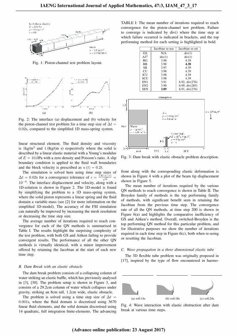
Fig. 1: Piston-channel test problem layout.

(a) (b)

Fig. 2: The interface (a) displacement and (b) velocity forthe piston-channel test problem for a time step size of ∆t =0.02s, compared to the simplified 1D mass-spring system.

linear structural element. The fluid density and viscosityis 1kg/m3 and 1.0kg/(m s) respectively where the solid isdescribed by a linear elastic material with a Young’s modulusof E = 10.0Pa with a zero density and Poisson’s ratio. A slipboundary condition is applied to the fluid wall boundariesand the block velocity is prescribed as u (t) = 0.2t.

The simulation is solved here using time step sizes of∆t = 0.02s for a convergence tolerance of ε =

||K(xsn)||√n

=

10−8. The interface displacement and velocity, along with a1D-solution is shown in Figure 2. The 1D-model is foundby simplifying the problem to a 1D mass-spring system,where the solid piston represents a linear spring and the fluiddomain a variable mass (see [2] for more information on thesimplified 1D-model). The accuracy of the FSI simulationcan naturally be improved by increasing the mesh resolutionor decreasing the time step size.

The average number of iterations required to reach con-vergence for each of the QN methods is summarised inTable I. The results highlight the surprising complexity ofthe test problem, with both GS and Aitken failing to provideconvergent results. The performance of all the other QNmethods is virtually identical, with a minor improvementoffered by retaining the Jacobian at the start of each newtime step.

B. Dam Break with an elastic obstacle

The dam break problem consists of a collapsing column ofwater striking an elastic baffle, which has previously analysedin [3], [30]. The problem setup is shown in Figure 3, andconsists of a 29.2cm column of water which collapses undergravity, striking an 8cm tall, 1.2cm wide, elastic obstacle.

The problem is solved using a time step size of ∆t =0.001s, where the fluid domain is discretised using 3670linear fluid elements, and the solid domain discretised using14 quadratic, full integration finite-elements. The advancing

TABLE I: The mean number of iterations required to reachconvergence for the piston-channel test problem. Failureto converge is indicated by div() where the time step atwhich failure occurred is indicated in brackets, and the topperforming method for each setting is highlighted in bold.

Jacobian re-use Jacobian re-setGS N/A div(1)Aδ2 div(1) div(1)BG 3.98 4.39BB 3.98 4.38SB 3.97 4.39CU 3.98 4.39ICU 3.98 4.39SCU 3.98 4.39EN1 3.91 6.92, div(276)EN2 3.90 6.99, div(285)SEN 3.89 6.91, div(276)

Fig. 3: Dam break with elastic obstacle problem description.

front along with the corresponding elastic deformation isshown in Figure 4 with a plot of the beam tip displacementshown in Figure 5.

The mean number of iterations required by the variousQN methods to reach convergence is shown in Table II. TheBroyden family of methods is the top performing familyof methods, with significant benefit seen in retaining theJacobian from the previous time step. The convergencerate of all the QN methods, at time step 200 is shown inFigure 6(a) and highlights the comparative inefficiency ofGS and Aitken’s method. Overall, switched-Broyden is thetop performing QN method for this particular problem, andfor illustrative purposes we show the number of iterationsrequired in each time step in Figure 6(c), both when re-usingor resetting the Jacobian.

C. Wave propagation in a three dimensional elastic tube

The 3D flexible tube problem was originally proposed in[17], inspired by the type of flow encountered in haemo-

(a) t=0.14s (b) t=0.18s (c) t=0.24s

Fig. 4: Wave interaction with elastic obstruction after dambreak at various time steps.



______________________________________________________________________________________

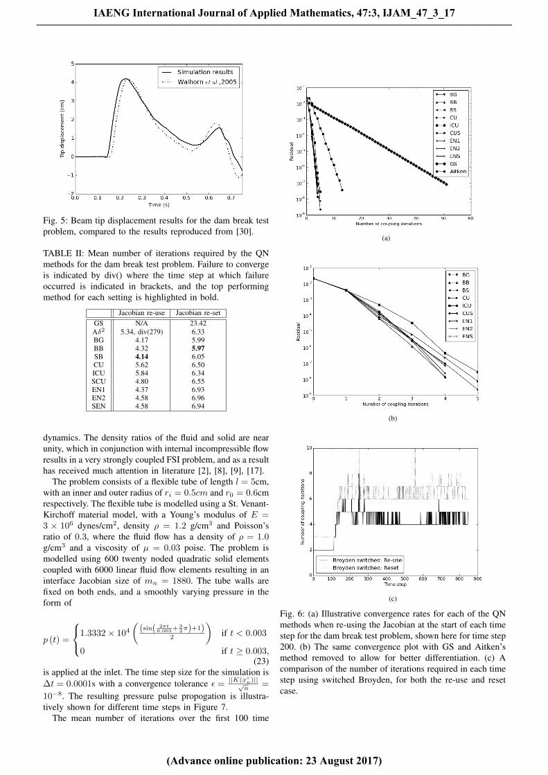
Fig. 5: Beam tip displacement results for the dam break testproblem, compared to the results reproduced from [30].

TABLE II: Mean number of iterations required by the QNmethods for the dam break test problem. Failure to convergeis indicated by div() where the time step at which failureoccurred is indicated in brackets, and the top performingmethod for each setting is highlighted in bold.

Jacobian re-use Jacobian re-setGS N/A 23.42Aδ2 5.34, div(279) 6.33BG 4.17 5.99BB 4.32 5.97SB 4.14 6.05CU 5.62 6.50ICU 5.84 6.34SCU 4.80 6.55EN1 4.37 6.93EN2 4.58 6.96SEN 4.58 6.94

dynamics. The density ratios of the fluid and solid are nearunity, which in conjunction with internal incompressible flowresults in a very strongly coupled FSI problem, and as a resulthas received much attention in literature [2], [8], [9], [17].

The problem consists of a flexible tube of length l = 5cm,with an inner and outer radius of ri = 0.5cm and r0 = 0.6cmrespectively. The flexible tube is modelled using a St. Venant-Kirchoff material model, with a Young’s modulus of E =3 × 106 dynes/cm2, density ρ = 1.2 g/cm3 and Poisson’sratio of 0.3, where the fluid flow has a density of ρ = 1.0g/cm3 and a viscosity of µ = 0.03 poise. The problem ismodelled using 600 twenty noded quadratic solid elementscoupled with 6000 linear fluid flow elements resulting in aninterface Jacobian size of mn = 1880. The tube walls arefixed on both ends, and a smoothly varying pressure in theform of

p (t) =

1.3332× 104(

(sin( 2πt0.003+

32π)+1)

2

)if t < 0.003

0 if t ≥ 0.003,(23)

is applied at the inlet. The time step size for the simulation is∆t = 0.0001s with a convergence tolerance ε =

||K(xsn)||√n

=

10−8. The resulting pressure pulse propogation is illustra-tively shown for different time steps in Figure 7.

The mean number of iterations over the first 100 time

(a)

(b)

(c)

Fig. 6: (a) Illustrative convergence rates for each of the QNmethods when re-using the Jacobian at the start of each timestep for the dam break test problem, shown here for time step200. (b) The same convergence plot with GS and Aitken’smethod removed to allow for better differentiation. (c) Acomparison of the number of iterations required in each timestep using switched Broyden, for both the re-use and resetcase.



______________________________________________________________________________________

Fig. 7: Pressure pulse propagation at 0.003s, 0.005s and0.008s (where the wall displacement is magnified by a factor10).

TABLE III: Comparison of the mean number of iterationsrequired to reach convergence for the 3D flexible tube testproblem. Failure to converge is indicated by div() where thetime step at which failure occurred is indicated in brackets,and the top performing method for each setting is highlightedin bold.

Jacobian re-use Jacobian re-setGS N/A div(1)Aδ2 div(1) div(1)BG 6.51 15.36BB 7.68 22.25SB 6.75 15.38CU 15.63 17.51ICU 27.21, div(14) 27.64, div(22)SCU 13.89 17.62EN1 6.91 20.56EN2 10.56 16.83, div(26)SEN 7.37 20.63

steps is shown in Table III for the various QN methods. TheBroyden family of methods is once again the top performingmethod, with a clear benefit in retaining the old Jacobianat the start of each time step. A summary of the numberof coupling iterations required per time step, for each ofthe family of methods, is shown in Figure 8. Out of all thetest cases analysed in this paper, this problem most clearlyhighlights the inherent training that occurs by retaining andcontinuously adding onto the Jacobian. To further illustratethis inherent training, we show the convergence rates forBroyden’s good method in Figure 9 at different time stepsfor both re-use and resetting of the Jacobian.

D. 2D flexible beam fluid-structure interactions

The selected test problem consists of flow around a fixedcylinder with an attached flexible beam. The beam undergoeslarge deformations induced by oscillating vortices formed byflow around the circular bluff body. The problem was firstproposed by Turek et al. [29], and has received substantialnumerical verification.

The problem layout and material properties are providedin Figure 10(a) and consists of a 0.02m thick, 0.35m longflexible beam, attached to a fixed cylinder with diameterof 0.1m. The cylinder center is by design positioned tobe non-symmetric with respect to the channel to remove

(a)

(b)

(c)

Fig. 8: A comparison of the number of coupling iterationsrequired to reach convergence for the 3D flexible tubetest problem when using (a) Broyden’s family of methods,(b) Column updating family of methods and (c) Eirola-Nevanlinna family of methods when re-using the Jacobianfrom the previous time step and when resetting the Jacobianto −I .



______________________________________________________________________________________

(a)

(b)

Fig. 9: Illustrative convergence rates at various time stepsfor the 3D flexible tube test problem using Broyden’s Goodmethod when (a) re-using the Jacobian at the start of eachtime step and (b) when re-setting the Jacobian to −I at thestart of the new time step.

dependence on numerical errors to induce the onset ofdeformations. A parabolic inlet boundary condition, withmean flow velocity of U = 1m/s is slowly ramped upfor t < 0.5s via (1− cos (πt/2)) /2. The top, bottom andfixed cylinder walls are defined as non-slip boundaries. Theproblem is solved here using 3800 finite-volume fluid cells,and 72 full integration, quadratic finite elements.

We investigate three different settings, namely for a com-paratively large time step size of ∆t = 0.01s for two differentconvergence criteria of ε = 10−5 and ε = 10−8 in orderto gain some insight into the convergence behaviour of thevarious QN methods as well as for a small time step size of∆t = 0.001s for ε = 10−8. The beam tip displacement forboth time step sizes over the full simulation window is shownin Figure 10(b) with a snapshot of the beam displacementat 8.7s shown in Figure 10(c). The convergence behaviourfor the various QN methods is summarised in Tables IV-Table V. Overall, switched Broyden outperforms all the QNmethods across all three settings, with the switched strategiesproviding improved performance for both the conventionalEN and CU methods.

(a)

(b)

(c)

Fig. 10: (a) Flexible beam problem description, (b) beam tipdisplacement over the 10s simulation window, and (c) beamdisplacement and pressure contours at 8.7 seconds.

TABLE IV: The mean number of iterations to reach con-vergence for the flexible tail benchmark problem for thevarious QN methods when the Jacobian is re-used. Failureto converge is indicated by div() where the time step atwhich failure occurred is indicated in brackets, and the topperforming method for each setting is highlighted in bold.

∆t = 0.01, ∆t = 0.01, ∆t = 0.001,ε = 10−5 ε = 10−8 ε = 10−8

GS div(1) div(1) div(1)Aδ2 3.51 10.31 div(4)BG 2.938 4.017 4.407BB 3.039 4.250 4.480BS 2.906 3.983 4.024CU 3.342 5.264 -(1581)ICU 3.108 5.391 8.388CUS 2.975 4.836 6.025EN1 3.192 4.614 5.443EN2 3.147 4.543 5.854ENS 3.137 4.535 4.920

V. CONCLUSION

We have tested a wide variety of acceleration techniqueson four different multi-physics problems that are written asa fixed-point problem. While the choice of the best methodremains problem dependent, it is clear that the best choiceis the class of quasi-Newton methods, of which, more oftenthan not, the tried and trusted Broyden method comes outon top.Re-using the Jacobian of all the QN methods at the beginningof the iterations of the next time step results in importantreductions in the required number of iterations. With a fewexceptions, a switching strategy, that hasn’t drawn muchattention in the past, is shown to offer a slight boost of perfor-mance in exchange for a negligeable penalty in complexity.The class of Eirola-Nevanlinna methods, which are among



______________________________________________________________________________________

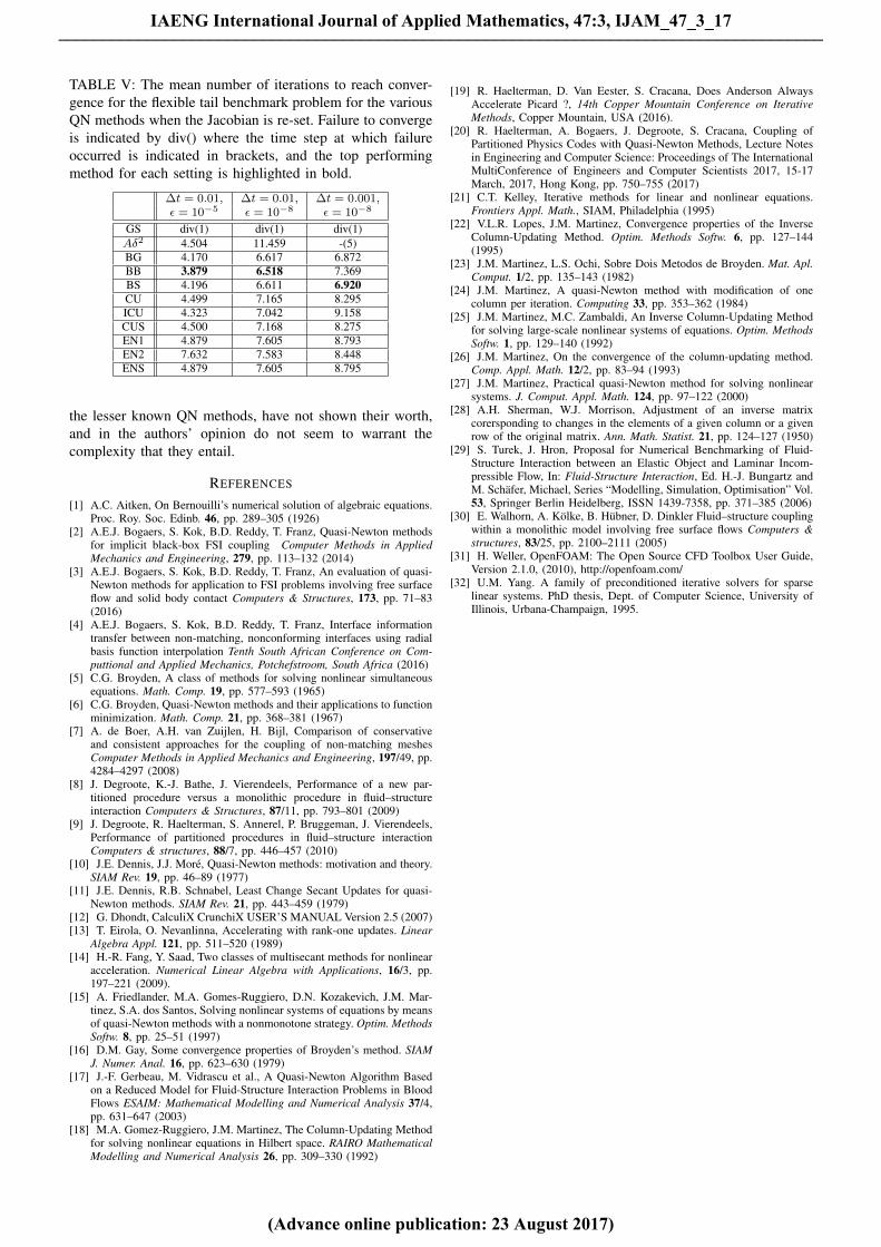
TABLE V: The mean number of iterations to reach conver-gence for the flexible tail benchmark problem for the variousQN methods when the Jacobian is re-set. Failure to convergeis indicated by div() where the time step at which failureoccurred is indicated in brackets, and the top performingmethod for each setting is highlighted in bold.

∆t = 0.01, ∆t = 0.01, ∆t = 0.001,ε = 10−5 ε = 10−8 ε = 10−8

GS div(1) div(1) div(1)Aδ2 4.504 11.459 -(5)BG 4.170 6.617 6.872BB 3.879 6.518 7.369BS 4.196 6.611 6.920CU 4.499 7.165 8.295ICU 4.323 7.042 9.158CUS 4.500 7.168 8.275EN1 4.879 7.605 8.793EN2 7.632 7.583 8.448ENS 4.879 7.605 8.795

the lesser known QN methods, have not shown their worth,and in the authors’ opinion do not seem to warrant thecomplexity that they entail.

REFERENCES

[1] A.C. Aitken, On Bernouilli’s numerical solution of algebraic equations.Proc. Roy. Soc. Edinb. 46, pp. 289–305 (1926)

[2] A.E.J. Bogaers, S. Kok, B.D. Reddy, T. Franz, Quasi-Newton methodsfor implicit black-box FSI coupling Computer Methods in AppliedMechanics and Engineering, 279, pp. 113–132 (2014)

[3] A.E.J. Bogaers, S. Kok, B.D. Reddy, T. Franz, An evaluation of quasi-Newton methods for application to FSI problems involving free surfaceflow and solid body contact Computers & Structures, 173, pp. 71–83(2016)

[4] A.E.J. Bogaers, S. Kok, B.D. Reddy, T. Franz, Interface informationtransfer between non-matching, nonconforming interfaces using radialbasis function interpolation Tenth South African Conference on Com-puttional and Applied Mechanics, Potchefstroom, South Africa (2016)

[5] C.G. Broyden, A class of methods for solving nonlinear simultaneousequations. Math. Comp. 19, pp. 577–593 (1965)

[6] C.G. Broyden, Quasi-Newton methods and their applications to functionminimization. Math. Comp. 21, pp. 368–381 (1967)

[7] A. de Boer, A.H. van Zuijlen, H. Bijl, Comparison of conservativeand consistent approaches for the coupling of non-matching meshesComputer Methods in Applied Mechanics and Engineering, 197/49, pp.4284–4297 (2008)

[8] J. Degroote, K.-J. Bathe, J. Vierendeels, Performance of a new par-titioned procedure versus a monolithic procedure in fluid–structureinteraction Computers & Structures, 87/11, pp. 793–801 (2009)

[9] J. Degroote, R. Haelterman, S. Annerel, P. Bruggeman, J. Vierendeels,Performance of partitioned procedures in fluid–structure interactionComputers & structures, 88/7, pp. 446–457 (2010)

[10] J.E. Dennis, J.J. More, Quasi-Newton methods: motivation and theory.SIAM Rev. 19, pp. 46–89 (1977)

[11] J.E. Dennis, R.B. Schnabel, Least Change Secant Updates for quasi-Newton methods. SIAM Rev. 21, pp. 443–459 (1979)

[12] G. Dhondt, CalculiX CrunchiX USER’S MANUAL Version 2.5 (2007)[13] T. Eirola, O. Nevanlinna, Accelerating with rank-one updates. Linear

Algebra Appl. 121, pp. 511–520 (1989)[14] H.-R. Fang, Y. Saad, Two classes of multisecant methods for nonlinear

acceleration. Numerical Linear Algebra with Applications, 16/3, pp.197–221 (2009).

[15] A. Friedlander, M.A. Gomes-Ruggiero, D.N. Kozakevich, J.M. Mar-tinez, S.A. dos Santos, Solving nonlinear systems of equations by meansof quasi-Newton methods with a nonmonotone strategy. Optim. MethodsSoftw. 8, pp. 25–51 (1997)

[16] D.M. Gay, Some convergence properties of Broyden’s method. SIAMJ. Numer. Anal. 16, pp. 623–630 (1979)

[17] J.-F. Gerbeau, M. Vidrascu et al., A Quasi-Newton Algorithm Basedon a Reduced Model for Fluid-Structure Interaction Problems in BloodFlows ESAIM: Mathematical Modelling and Numerical Analysis 37/4,pp. 631–647 (2003)

[18] M.A. Gomez-Ruggiero, J.M. Martinez, The Column-Updating Methodfor solving nonlinear equations in Hilbert space. RAIRO MathematicalModelling and Numerical Analysis 26, pp. 309–330 (1992)

[19] R. Haelterman, D. Van Eester, S. Cracana, Does Anderson AlwaysAccelerate Picard ?, 14th Copper Mountain Conference on IterativeMethods, Copper Mountain, USA (2016).

[20] R. Haelterman, A. Bogaers, J. Degroote, S. Cracana, Coupling ofPartitioned Physics Codes with Quasi-Newton Methods, Lecture Notesin Engineering and Computer Science: Proceedings of The InternationalMultiConference of Engineers and Computer Scientists 2017, 15-17March, 2017, Hong Kong, pp. 750–755 (2017)

[21] C.T. Kelley, Iterative methods for linear and nonlinear equations.Frontiers Appl. Math., SIAM, Philadelphia (1995)

[22] V.L.R. Lopes, J.M. Martinez, Convergence properties of the InverseColumn-Updating Method. Optim. Methods Softw. 6, pp. 127–144(1995)

[23] J.M. Martinez, L.S. Ochi, Sobre Dois Metodos de Broyden. Mat. Apl.Comput. 1/2, pp. 135–143 (1982)

[24] J.M. Martinez, A quasi-Newton method with modification of onecolumn per iteration. Computing 33, pp. 353–362 (1984)

[25] J.M. Martinez, M.C. Zambaldi, An Inverse Column-Updating Methodfor solving large-scale nonlinear systems of equations. Optim. MethodsSoftw. 1, pp. 129–140 (1992)

[26] J.M. Martinez, On the convergence of the column-updating method.Comp. Appl. Math. 12/2, pp. 83–94 (1993)

[27] J.M. Martinez, Practical quasi-Newton method for solving nonlinearsystems. J. Comput. Appl. Math. 124, pp. 97–122 (2000)

[28] A.H. Sherman, W.J. Morrison, Adjustment of an inverse matrixcorersponding to changes in the elements of a given column or a givenrow of the original matrix. Ann. Math. Statist. 21, pp. 124–127 (1950)

[29] S. Turek, J. Hron, Proposal for Numerical Benchmarking of Fluid-Structure Interaction between an Elastic Object and Laminar Incom-pressible Flow, In: Fluid-Structure Interaction, Ed. H.-J. Bungartz andM. Schafer, Michael, Series “Modelling, Simulation, Optimisation” Vol.53, Springer Berlin Heidelberg, ISSN 1439-7358, pp. 371–385 (2006)

[30] E. Walhorn, A. Kolke, B. Hubner, D. Dinkler Fluid–structure couplingwithin a monolithic model involving free surface flows Computers &structures, 83/25, pp. 2100–2111 (2005)

[31] H. Weller, OpenFOAM: The Open Source CFD Toolbox User Guide,Version 2.1.0, (2010), http://openfoam.com/

[32] U.M. Yang. A family of preconditioned iterative solvers for sparselinear systems. PhD thesis, Dept. of Computer Science, University ofIllinois, Urbana-Champaign, 1995.



______________________________________________________________________________________

Documents

Quasi-Newton Methods for the Acceleration of Multi … · Quasi-Newton Methods for the Acceleration of Multi-Physics Codes Rob Haelterman, Alfred Bogaers, Joris Degroote, Nicolas