Quasi-Lagrangian Large Eddy Simulations of Cross ... · PDF fileQuasi-Lagrangian Large Eddy Simulations of Cross-Equatorial Flow in the East Paciﬁc Atmospheric Boundary Layer

VOL. 61, NO. 15 1 AUGUST 2004J O U R N A L O F T H E A T M O S P H E R I C S C I E N C E S

q 2004 American Meteorological Society 1837

Quasi-Lagrangian Large Eddy Simulations of Cross-Equatorial Flow in the East PacificAtmospheric Boundary Layer

S. P. DE SZOEKE AND C. S. BRETHERTON

Department of Atmospheric Sciences, University of Washington, Seattle, Washington

(Manuscript received 8 August 2003, in final form 17 December 2003)

ABSTRACT

Using a large eddy simulation (LES), the atmospheric boundary layer (ABL) is numerically modeled along958W from 88S to 48N during boreal autumn, and compared to observations from the East Pacific Investigationof Climate Processes in the Coupled Ocean–Atmosphere System (EPIC) 2001. Since the local ABL winds arepredominantly southerly in this season, a ‘‘quasi-Lagrangian’’ forcing is used in which the ABL air column isforced as if it were advecting northward with the mean September–October 2001 meridional wind across theequatorial cold tongue and the rapidly warming SSTs to the north. Pressure gradients and large-scale zonaladvective tendencies are prescribed as a function of latitude. Where possible, observations from the EPIC 2001experiment are used for forcing and for comparison with model results.

The ABL’s modeled vertical structure accords with the conceptual model of Wallace et al. and agrees wellwith observations. Surface stability accounts for the minimum in surface wind over the equatorial cold tongueand the maximum over the warm water to the north. Stability of the lower ABL over the cold tongue allows ajet to accelerate at about 500-m height, relatively uncoupled to the frictional surface layer. Vertical mixing overthe warm water to the north distributes this momentum to the surface.

Additional simulations were performed to explore the modeled ABL’s sensitivity to pressure gradients, zonaladvection, free-tropospheric humidity, and initial conditions. The model ABL was robust: changing the forcingsresulted in little change in the modeled structure. The strongest sensitivity was of stratocumulus clouds overthe cold tongue to cloud-top radiative cooling. Once formed at the southern edge of the cold tongue, modeledstratocumulus clouds demonstrate a remarkable ability to maintain themselves over the cold tongue in the absenceof surface fluxes by radiative cooling at their tops. The persistence of thin stratocumulus clouds in this Lagrangianmodel suggests that horizontal advection of condensate might be an important process in determining cloudinessover the cold tongue.

1. Introduction

Processes that affect surface winds in the Tropics areadvection of momentum, surface pressure gradients(Deser 1993), momentum fluxes through the top of theABL (e.g., Stevens et al. 2002), and efficiency of tur-bulent vertical mixing within the ABL. Lindzen andNigam (1987) noted that above warm SST, lower-tro-pospheric air temperature is warm, hydrostatically in-ducing low surface pressure. The corresponding hori-zontal pressure gradients induce horizontal wind con-vergence over warm SST, explaining the large-scale dis-tribution of precipitation over the Tropics. According tothe Lindzen–Nigam theory, winds near the equatorshould be particularly strong over large SST gradients,such as the winds seen over the eastern equatorial Pacificduring boreal fall.

Wallace et al. (1989, hereafter WMD) suggested thatin this region, vertical mixing within the ABL also mod-

Corresponding author address: S. P. de Szoeke, Dept. of Atmo-spheric Sciences, University of Washington, Seattle, WA 98195.E-mail: [email protected]

ulates the coupling of surface wind to SST. Especiallyin July–December, a large-scale meridional pressuregradient in the east Pacific causes cross-equatorial ABLflow, while oceanic upwelling creates a tongue of coldwater along the equator. WMD found that surface windsreported in a climatology of routine ship observationswere strongest over the warm water to the north of thestrongest SST gradients. They proposed that the surfacewind is stronger where the SST is significantly warmerthan the surface air temperature (an unstable surfacelayer), because turbulent convection efficiently mixesmomentum down to the surface. Conversely, over coldSST, the surface layer is more stable and inhibits down-ward turbulent mixing of momentum, weakening thesurface wind. The signature of the stability effect on thesurface wind is horizontal divergence across (positivedownwind) SST gradients.

Hayes et al. (1989) and Thum et al. (2002), usingTropical Atmosphere Ocean (TAO) buoy observations,and Chelton et al. (2001), using satellite observations,showed how surface wind variations in this region cor-related with meandering of the pronounced equatorial

1838 VOLUME 61J O U R N A L O F T H E A T M O S P H E R I C S C I E N C E S

front in SST associated with tropical instability waves.These correlations were consistent with the mechanismof WMD. Also consistent with the WMD mechanism,Bond (1992) used radiosonde observations taken duringTAO buoy maintenance cruises to show a lower surfacewind speed and an elevated wind jet in the ABL overthe cold tongue, and increased surface wind speed withvertically homogeneous winds within the ABL over thewarm water north of the SST front. Hashizume et al.(2002) found similar results from a research cruise thatcut zonally through several meanders of the SST front.

During September–October 2001, the East Pacific In-vestigation of Climate Processes in the Coupled Ocean–Atmosphere System (EPIC) 2001 field campaign madeintensive measurements of the atmospheric and oceanicstructure along the easternmost line of TAO buoys at958W (Raymond et al. 2004). One goal of these mea-surements was to provide a comprehensive view of themean ABL structure and its day-to-day variability in thecross-equatorial flow region. By combining airborne,ship-based, and TAO buoy measurements, EPIC 2001for the first time documented the ABL turbulence, cloudstructures and microphysics, radiative flux profiles, andinstantaneous downwind evolution over a representativerange of atmospheric conditions. This provides an ex-cellent opportunity to extend WMD’s ideas into a rig-orous, quantitative test of ABL models and general cir-culation model (GCM) parameterizations in this chal-lenging and climatically important region.

In this paper, we adopt the large eddy simulation(LES) as a natural modeling approach for better un-derstanding the eastern equatorial Pacific ABL, and forinterpreting and comparing with the EPIC 2001 obser-vations. Because the largest turbulent structures are re-solved, the LES framework is capable of simulating theinteractions of surface fluxes, turbulence, clouds, andradiation that contribute to the vertical structure of theABL and its south-to-north evolution. Using a ‘‘quasi-Lagrangian’’ LES approach described in section 2, wesimulate ABL evolution along 958W, starting at 88S inthe southeast Pacific stratocumulus region (Brethertonet al. 2004), traversing the cold tongue and the equa-torial SST front, and ending at 48N in the shallow cu-mulus region upstream of the intertropical convergencezone. We compare our simulations with EPIC 2001 ob-servations (section 3), and present sensitivity studies(section 4), followed by discussion and conclusions(section 5). The LES is consistent with WMD, but itelucidates several other feedbacks that may affect thevertical structure and temporal variability of the ABLcross-equatorial flow. Our quasi-Lagrangian LES mod-els the thermodynamic evolution and vertical structureof the ABL well, but pressure gradients are prescribedand do not respond to the evolving ABL.

2. MethodsWe integrated an LES on a 3-km cubic domain with

enough resolution to resolve turbulent eddies 100 m or

more across. The LES was forced in a quasi-Lagrangianmanner, by time-varying conditions (notably underlyingSST, large-scale pressure gradients, and overlying free-tropospheric temperature and humidity) that correspondto the northward movement undergone by a typicalboundary layer air column. The simulation can then beunderstood as tracing the boundary layer column’s evo-lution with time or latitude as the column moves along958W. Section 2a describes the quasi-Lagrangian frame-work and how the external forcings are applied to theLES. Section 2b describes how observations and re-analysis are used to determine these latitude-dependentexternal forcings. Section 2c describes the details of theLES model.

a. Quasi-Lagrangian method

Our quasi-Lagrangian forcing strategy was inspiredby Wakefield and Schubert (1981), Wyant et al. (1997),and Bretherton et al. (1999a). A meridional ABL tra-jectory (latitude versus time) was computed from theSeptember–October 2001 National Centers for Envi-ronmental Predicition (NCEP) mean 1000–925-hPawind, which we assume to represent the mean meridi-onal ABL wind. Along this trajectory, it takes 3 daysto get from 88S to 48N. Our strategy capitalizes on thepredominantly southerly winds near the equator and theweak zonal gradient of SST compared to the meridionalgradient. This ensures that advective tendencies are pri-marily due to the meridional wind. To simplify the mod-el and facilitate comparison with EPIC 2001 observa-tions—which were all along a single longitude—we ne-glected the zonal velocity from the Lagrangian advec-tive wind speed. The idealized Lagrangian trajectory isa straight northward path along 958W longitude. Large-scale meridional advection is built into this Lagrangiancolumn-following formulation, while large-scale zonaladvection is computed from the NCEP reanalysis andthen applied to the LES in an Eulerian fashion.

In the quasi-Lagrangian formulation, the entire col-umn is assumed to move at the mean ABL meridionalvelocity. A shortcoming of this method is that it doesnot simulate the effect of differential meridional ad-vection at different heights within the ABL. If there isvertical shear in the boundary layer, then air movingfaster or slower than the vertical mean could contributean advective tendency into the ABL column. In the LES,even though the layers are free to move at differentspeeds, the small domain and periodic lateral boundariesprevent differential advection into the column. Thisshortcoming is of minimal importance as long as theboundary layer is mixed, because in this case the ve-locities do not change with height. To the extent thatthe ABL is not well mixed, differential advection wouldhave an effect not simulated by the quasi-Lagrangianmethod. While the ABL evolution is predicted in oursimulation, the free troposphere is merely specified asan upper boundary condition for the ABL by relaxing

1 AUGUST 2004 1839D E S Z O E K E A N D B R E T H E R T O N

it to a specified profile on an hourly time scale. Exter-nally relaxing the free troposphere provides for the ef-fect of differential meridional advection between theABL and the free troposphere.

The evolution of the vertical structure of the boundarylayer is predicted by the LES as if it were a turbulence-resolving column model, with horizontally homoge-neous large-scale forcings. We use the Ogura and Phil-lips (1962) anelastic equations to describe motions with-in the column. These are based on hydrostatic profilesof reference pressure p0(z) and density r0(z) calculatedassuming a constant reference potential temperature u00

5 302.1 K and a reference surface pressure p0(0) 51012.8 hPa:

Du u9y u u5 g k 2 =f9 2 fk 3 u 1 S 1 SLS sfcDt u00

11 = · r K =u, (1)0 Mr 0

Du 1 ]l u u ul l l5 S 2 F 1 S 1 Smicro rad LS sfcDt r C P ]z0 P 0

11 = · r K =u , (2)0 H lr 0

Dq 1t q q qt t t5 S 1 S 1 S 1 = · r K =q , (3)micro LS sfc 0 H tDt r 0

Dq ]qr rqt5 2S 2 w , (4)micro rDt ]z

= · (r u) 5 0. (5)0

The left-hand side of Eqs. (1)–(4) are the Lagrangiantime derivatives of velocity u, liquid water potentialtemperature ul, water mixing ratio qt (including vaporand cloud liquid), and rain water mixing ratio qr. Primesindicate the deviation of a quantity from its horizontalmean. The Coriolis force 2 fk 3 u is computed ex-plicitly by the LES. The heat source due to evaporationand condensation of cloud water does not appear be-cause the equations have been formulated in terms ofliquid water potential temperature,

u 5 u 2 (L/P C )q ,l 0 p l (6)

where u is the potential temperature, L is the latent heatof vaporization of water, P0 is the base-state Exner func-tion, Cp is the specific heat of air, and ql is the cloudliquid water. There is, however, a ul source , andulSmicro

a corresponding qt sink when precipitation formsqtSmicro

from cloud liquid water, or evaporates (detailed in sec-tion 2c). The source Ssfc due to the surface flux is de-posited entirely in the lowest model level. The radiativeflux convergence 2]Frad/]z is calculated columnwise bya radiative transfer model within the LES. The last termsin Eqs. (1)–(3) are the subgrid-scale diffusion of mo-mentum, heat, and moisture. The subgrid eddy viscosityis denoted KM and KH is the eddy diffusivity of heat

and moisture. Anelastic mass continuity is expressed by(5).

We denote specified latitude and height-dependentquantities derived from EPIC 2001 or NCEP by a hat,and denote horizontally domain-averaged quantities pre-dicted by the LES by an overbar. Then the large-scaleforcings are given by

(u 2 u) ]u ]uuS 5 H(z 2 z ) 2 u 2 w 2 =f, (7)LS relax t ]x ]z

(u 2 u ) ]u ]ul l l lulS 5 H(z 2 z ) 2 u 2 w , and (8)LS relax t ]x ]z

(q 2 q ) ]q ]qt t t tqtS 5 H(z 2 z ) 2 u 2 w . (9)LS relax t ]x ]z

The first terms in the large-scale forcing Eqs. (7)–(9)are the relaxation of the mean to the prescribed soundingabove the ABL. The Heaviside function H(z 2 zrelax) isunity above the relaxation height zrelax and zero below.The relaxation height

z 5 z 1 150 m (10)relax inv

is defined as 150 m above the horizontal mean inversionheight. In each column the inversion height zinv is de-fined to be the height of maximum stability ]uy/]z. Ashort relaxation time scale, arbitrarily chosen as t 5 1 h,keeps the free troposphere close to the specified ther-modynamic and wind profiles above the relaxationheight. The relaxation height was chosen to be as closeas possible to the inversion while still remaining abovethe maximum height of inversion-penetrating turbulenteddies. This ensures the free-tropospheric air entrainedinto the boundary layer has the desired specified ther-modynamic characteristics, but does not distort the in-version structure. A similar procedure was used byWyant et al. (1997).

The large-scale zonal advection 2u]()/]x and pres-sure gradient term 2= are computed from NCEP re-fanalysis. The vertical advection 2w] /]z is due to the( )imposed subsidence velocity w. The mean subsidenceis incorporated in the LES by applying vertical advec-tive tendencies to the prognosed quantities of l, t,u q

, and , without changing the LES-predicted verticalu yvelocity (which always has zero horizontal mean). Thelarge-scale meridional advection is accounted for by thequasi-Lagrangian boundary conditions on the LES.

b. Large-scale forcing

The required time-dependent forcings on the LES are1) sea surface temperature; 2) zonal advection; 3) pres-sure gradient force; 4) subsidence rate; and 5) free-tro-pospheric profiles of temperature, humidity, and wind.We composited the SST from the Tropical Rainfall Mea-suring Mission (TRMM) Microwave Imager (TMI) av-erage satellite retrievals for 30 September–2 October2001, and 5-cm-deep temperatures measured from the


FIG. 1. SST along 958W measured by two partial RHB transects,30 Sep–2 Oct 2001 average TMI observations, and Sep–Oct 2001mean TAO buoy observations. The line labeled LES BC is the bound-ary condition used for the LES.

National Oceanic and Atmospheric Administration’s(NOAA) R/V Ronald H. Brown (RHB; see Fig. 1). TheTMI SST is smooth compared to the RHB SST, whichwas sampled during a single southward transect (therebyconvolving spatial and temporal variability). The thingray line in Fig. 1 shows the composite SST that weused for LES integration. It mostly follows the TMIretrieval, but near 0.58N, we have chosen to sharpen theidealized SST front in agreement with the observationsfrom the RHB (thin lines). We do this because we regardour simulation as one typical realization of ABL evo-lution over a sharp SST front, not as a 2-month com-posite averaging over all the day-to-day oceanic andatmospheric variability.

Zonal advection and large-scale pressure gradientforces are computed from the September–October 2001mean NCEP reanalysis. They are computed at the levelsavailable in the NCEP reanalysis dataset: the surface,1000, 925, 850, and 700 hPa. The sea level pressuregradient force 2 =p(0) is used at the surface, while21r 0

the geopotential height gradient 2=f is used at thereanalysis pressure levels. The geopotential gradientsare assigned a nominal altitude and interpolated in z tothe model grid levels. The large-scale zonal pressuregradient force 2] /]x is computed with a centered dif-fference of geopotential between 92.58 and 97.58W. Thelarge-scale meridional pressure gradient force 2] /]yfis computed from the difference of the geopotential at2.58 latitude intervals (. . . , 22.58, 08, 2.58, . . .) along958W. The meridional geopotential gradients are cen-tered in between (. . . , 21.258, 1.258, . . .) and thenlinearly interpolated in y to all latitudes to provide acontinuous forcing. This procedure yields a cross sec-

tion of large-scale forcings that depend on latitude y andaltitude z.

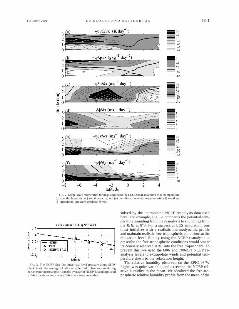
Figure 2 shows these forcing terms. The effect ofzonal temperature and moisture advection (Figs. 2a,b)is to cool and dry the near surface air. In the south,there is a considerable zonal component to the SSTgradient. The easterly wind component advects air thathas been in contact with the cool upwelled water alongthe South American coast. Over the cold tongue, wherethe air–sea temperature difference is positive, the ad-vective cooling and drying is small but significant, be-cause other thermal forcings are small.

The zonal pressure gradient (Fig. 2d) and zonal ad-vection of zonal momentum (Fig. 2c) combine to pro-duce systematic eastward acceleration of the northward-moving ABL air. The meridional pressure gradient inFig. 2f is strongest at the surface. Combined with themuch weaker zonal advection of y (Fig. 2e), it accel-erates ABL air to the north. In Fig. 3 the NCEP Sep-tember–October mean surface pressure along 958W(used to calculate the gradient at the surface in Fig. 2f)is compared to TAO surface pressure observations (tri-angles) for this period. Sampling is not continuous forthe TAO moorings. We tried to compensate for samplingby interpolating the NCEP data to the location of theTAO buoys, and averaging the NCEP data only on thosedays in September and October when the TAO buoysreported surface pressure. This method results in littleimprovement in the agreement between the TAO andNCEP surface pressures, indicating that small discrep-ancies not related to sampling exist between the twodatasets.

Mean vertical motion is an important forcing forboundary layer evolution. It is difficult to deduce fromthe type of in situ observations taken in EPIC 2001, sowe turned to NCEP reanalysis. According to the Sep-tember–October 2001 mean reanalysis, subsidence at700 hPa in the region between 88S and the equator wasabout 4 mm s21, and less to the north. This agrees withthe rate of descent of plumes of moisture observed bythe 3-hourly balloon soundings launched from the shipat 88S (Bretherton et al. 2004). In our simulation, wespecified a mean subsidence of w 5 24 mm s21 abovethe relaxation height at all latitudes. Below zrelax, thesubsidence linearly decreased to zero at the surface. Weregard the decrease in NCEP subsidence north of thecold tongue to be due to occasional deep convection inthe region. Since such deep convection is rarely seensouth of 48N, we felt it appropriate to use a subsidencerate consistent with radiative subsidence balance evennorth of the equator.

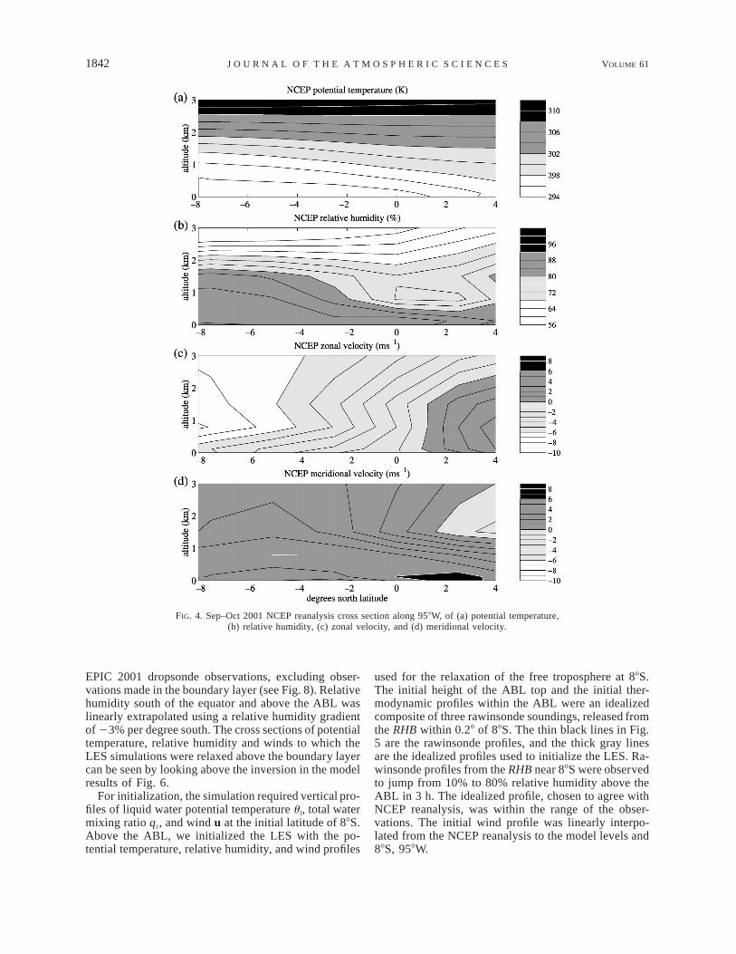
September–October 2001 mean NCEP reanalysis wasused to provide the free-tropospheric winds and tem-perature as a function of latitude. Figure 4 shows thepotential temperature, relative humidity, and zonal andmeridional wind from September–October 2001 NCEPreanalysis from 88S to 48N. The temperature structureup through the ABL capping inversion is not well re-


FIG. 2. Large-scale momentum forcings applied to the LES: Zonal advection of (a) temperature,(b) specific humidity, (c) zonal velocity, and (e) meridional velocity, together with (d) zonal and(f ) meridional pressure gradient forces.

FIG. 3. The NCEP Sep–Oct mean sea level pressure along 958W(black line), the average of all available TAO observations duringthe same period (triangles), and the average of NCEP data interpolatedto TAO locations only when TAO data were available.

solved by the interpolated NCEP reanalysis data usedhere. For example, Fig. 5a compares the potential tem-perature sounding from the reanalysis to soundings fromthe RHB at 88S. For a successful LES simulation, onemust initialize with a realistic thermodynamic profileand maintain realistic free-tropospheric conditions at therelaxation level. Simply using the NCEP reanalysis toprescribe the free-tropospheric conditions would smearits coarsely resolved ABL into the free troposphere. Toprevent this, we used the 600- and 700-hPa NCEP re-analysis levels to extrapolate winds and potential tem-perature down to the relaxation height.

The relative humidity observed on the EPIC 958Wflights was quite variable, and exceeded the NCEP rel-ative humidity in the mean. We idealized the free-tro-pospheric relative humidity profile from the mean of the


FIG. 4. Sep–Oct 2001 NCEP reanalysis cross section along 958W, of (a) potential temperature,(b) relative humidity, (c) zonal velocity, and (d) meridional velocity.

EPIC 2001 dropsonde observations, excluding obser-vations made in the boundary layer (see Fig. 8). Relativehumidity south of the equator and above the ABL waslinearly extrapolated using a relative humidity gradientof 23% per degree south. The cross sections of potentialtemperature, relative humidity and winds to which theLES simulations were relaxed above the boundary layercan be seen by looking above the inversion in the modelresults of Fig. 6.

For initialization, the simulation required vertical pro-files of liquid water potential temperature ul, total watermixing ratio qt, and wind u at the initial latitude of 88S.Above the ABL, we initialized the LES with the po-tential temperature, relative humidity, and wind profiles

used for the relaxation of the free troposphere at 88S.The initial height of the ABL top and the initial ther-modynamic profiles within the ABL were an idealizedcomposite of three rawinsonde soundings, released fromthe RHB within 0.28 of 88S. The thin black lines in Fig.5 are the rawinsonde profiles, and the thick gray linesare the idealized profiles used to initialize the LES. Ra-winsonde profiles from the RHB near 88S were observedto jump from 10% to 80% relative humidity above theABL in 3 h. The idealized profile, chosen to agree withNCEP reanalysis, was within the range of the obser-vations. The initial wind profile was linearly interpo-lated from the NCEP reanalysis to the model levels and88S, 958W.


FIG. 5. (a) Potential temperature and (b) relative humidity from rawinsondes released from the RHB near 88S on 12Oct 2001 (thin black lines). For comparison, the dotted line is the NCEP reanalysis, and the gray line is the initialcondition to the LES.

c. Large eddy simulation integration

The LES, called the Distributed Hydrodynamic Aero-sol and Radiation Model Application (DHARMA), hasa flux-limited, forward-in-time advection scheme (Ste-vens and Bretherton 1996). We ran DHARMA with pe-riodic horizontal boundary conditions, using a domainsize of 3.2 km 3 3.2 km in the horizontal and 3 km inthe vertical, and grid spacings of 50 m in the horizontaland 25 m in the vertical. This resolution required 64 364 3 120 grid points. Bretherton et al. (1999b) haveshown 10-m vertical resolution reduces the overpred-iction of entrainment made by 25-m resolution simu-lations in radiatively driven stratocumulus. We chose25-m resolution to accommodate the length of the in-tegration, and expect the overprediction of entrainmentto be less severe in the surface-driven ABL than inradiatively driven stratocumulus. The time step wasadaptive, aiming to maintain a target maximum Courantnumber maxi( | ui | Dt/Dxi) 5 0.5, where the maximumwas taken over the entire domain and all three velocitycomponents ui. The typical time step in our simulationwas 3 s. DHARMA’s parallel architecture allowed com-putations to be efficiently divided between multiple pro-cessors on a cluster of PCs. Using eight two-processornodes, an integration of three model days at this reso-lution took about 5 days.

The surface fluxes were computed by the CoupledOcean–Atmosphere Response Experiment (COARE)bulk flux algorithm (Fairall et al. 1996) from the prop-erties of the lowest resolved grid point (12.5 m) and theSST. The idealized SST in Fig. 1 was assumed to bethe skin temperature, so no additional skin temperatureadjustments were applied. For the purposes of calcu-lating the fluxes, the ocean surface current velocitieswere ignored.

Infrared and solar radiative fluxes were computed col-umnwise by BUGSrad (Stephens et al. 2001; Gabriel et

al. 2001), an 18-band two-stream radiative transfer mod-el developed for the Colorado State University GCM.Because of the computational expense of the radiationcalculation, it was performed only every 20 time steps.Additionally, in each time step the radiation was cal-culated for any column where cloud appeared in a gridcell where it had not been the previous time step, orwhere cloud disappeared from a grid cell where it hadbeen before. The downwelling solar flux, and the solarzenith angle at the top of the atmosphere were heldconstant. By reducing the solar constant by 1/2 to ac-count for the fraction of daylight, and using the daylight-average cosine of the solar zenith angle (correspondingto a zenith angle of 518), the constant solar flux used isequal to the expected diurnal-average of the solar fluxat the top of the atmosphere. Above the LES domain,the radiative transfer code uses a standard tropicalsounding of temperature and constituent concentrations.

DHARMA uses the bulk microphysical scheme ofWyant et al. (1997). Cloud liquid water qc is diagnosedfrom qt, ul, and r0 assuming zero supersaturation. Totalwater qt and liquid water potential temperature ul arenot changed by condensation or evaporation of cloudwater, so the only microphysical sources of qt and ul

are autoconversion and accretion of cloud water intorain water and evaporation of rain water. Autoconver-sion depends on qc and a specified cloud droplet con-centration, specified to be N 5 100 cm23. The verticalrain water flux is calculated by integrating the fall speedover the raindrop distribution. We use the subgrid-scalemoist turbulence scheme of Wyant et al. (1997), basedon Smagorinsky’s (1963) first-moment closure.

3. Baseline case results

Figure 6 shows time–height cross sections of potentialtemperature, relative humidity, and wind components


FIG. 6. Cross sections of the modeled cross-equatorial ABL from the BASE simulation. Theshading and contour intervals are the same as in Fig. 4. The conditions above the ABL are relaxedto the NCEP reanalysis in Fig. 4. The 99.9% relative humidity contour, shown by the thick whitecontour in (b) is an approximate indicator of the presence of cloud.

for a baseline simulation (BASE) that uses the forcingsand LES configuration described in section 2. The timeaxis (horizontally oriented in Fig. 6) can be interpretedequally well as latitude. We adopt this interpretation tofacilitate comparison with the EPIC 2001 observations.BASE captures much of the observed ABL evolutionalong 958W. The LES is not initialized with clouds, sothere are transient adjustments from the formation ofclouds in the first hours of model integration. After3 h, when the column has traversed to about 7.58S, theLES has completely spun up.

The modeled column simulates the two key transi-tions in the cross-equatorial ABL pointed out by WMD:the gradual formation of a stable layer over the equa-torial cold tongue and the rapid transition to a cumulus-under-stratocumulus boundary layer over the warm SST.Cross sections of the simulated potential temperature,relative humidity, and wind in the same format as theNCEP cross sections in Fig. 4 are presented in Fig. 6.Between 88 and 68S, the air–sea temperature differenceis negative, so surface latent and sensible heat fluxesprovide ample moisture for the clouds. As the column


FIG. 7. Potential temperature and meridional wind observations from dropsondes released during research flight 3show wind shear in the lower 300 m in the stable region over the equator (black). At 18N, the potential temperatureand momentum are mixed throughout the ABL (gray dashed).

goes north from 68S to the equator over progressivelycooler SST, the inversion lowers a little, and the cloudthins. The entrainment rate is we 5 3 mm s21, a littleweaker than the subsidence w 5 24 mm s21. Over thecoldest water, a stably stratified shear layer in both windcomponents forms within the ABL near the surface dueto the surface stability. Figure 7 shows profiles of po-tential temperature and meridional wind at the equatorand 18N, 958W measured by dropsondes released fromthe C-130 aircraft during EPIC 2001. The equatorialsounding shows the stability and wind shear in the low-est 300 m. Inefficient turbulent mixing within this layerleads to weak surface winds and greatly reduced surfacefluxes.

Starved of surface moisture flux, the modeled stra-tocumulus cloud nevertheless persists over the coldtongue, maintaining a delicate balance at the cloud topbetween radiative cooling and entrainment warming. Asecond transition takes place rapidly after the columncrosses the warm SST front. As suggested by WMD,over positive sensible and latent surface heat flux, thesurface stable layer is mixed out and the near-surfacewinds increase again. In this convective ABL, cumulusrising into stratocumulus clouds impinge on the inver-sion and rapidly deepen the boundary layer by entrain-ment. The inversion rises at a rate of 1.3 cm s21, im-plying an entrainment rate of we 5 1.7 cm s21. This islarger, but in qualitative agreement with estimates ofentrainment from heat and mass budgets derived fromthe EPIC 2001 observations along 958W (de Szoeke etal. 2004, manuscript submitted to J. Atmos. Sci.) and fromcoarse-scale observations of downstream deepening ofthe boundary layer (Wood and Bretherton 2004).

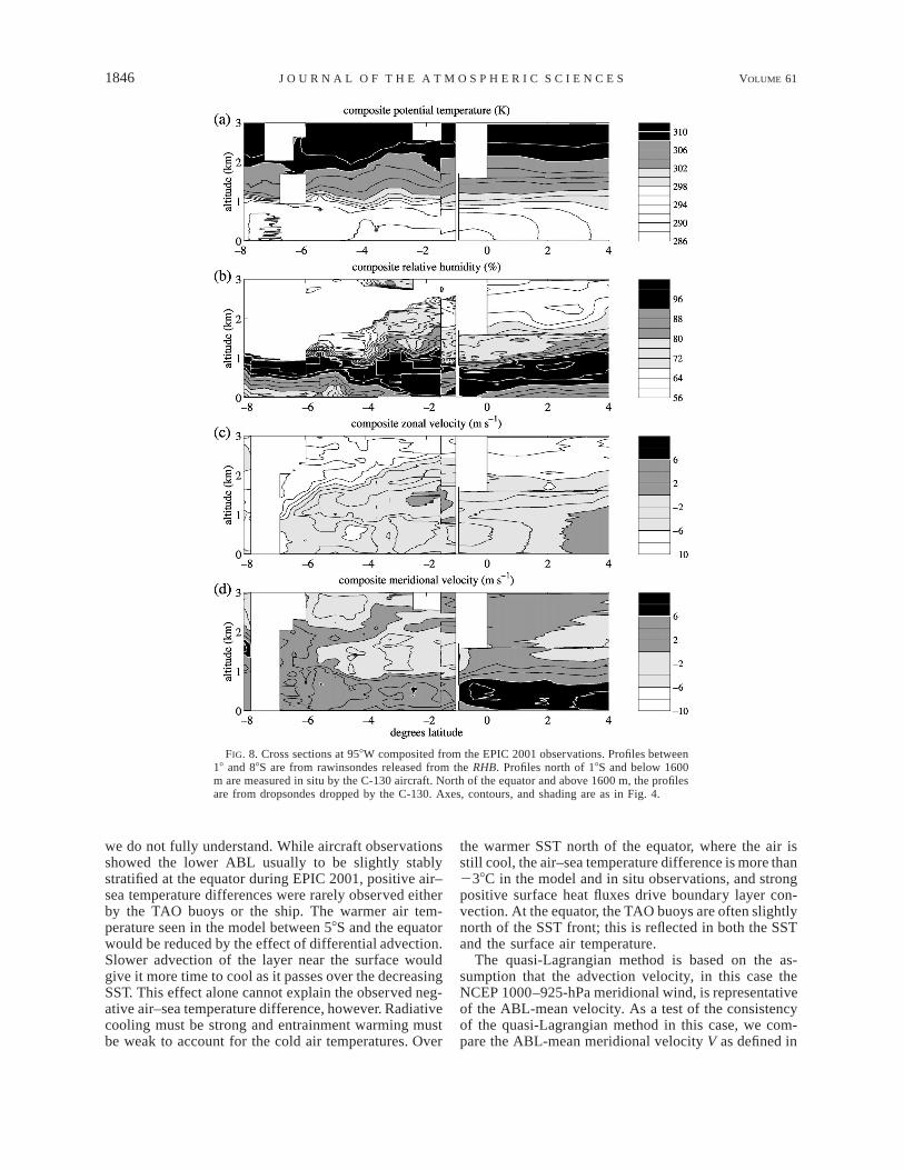
For comparison, Fig. 8 shows composite cross sec-tions of the atmosphere observed during EPIC 2001between 88S and 48N along 958W using all available insitu measurements. Between 88S and 28S, these are de-rived from rawinsondes released from a single transectof the RHB. Farther north we use an eight-flight mean

of in situ observations from the C-130 (18S–48N below1600 m), and dropsondes from the C-130 (08S–48Nabove 1600 m). The boundary layer capping inversion(the stable layer near 1000 m in Fig. 7a) rises slightlyand weakens in stability from the equator to 48N. Thecross sections of potential temperature for individualflights (not shown) resolve the inversion better than themean, because the averaging tends to blur the sharpfeatures sampled on each flight. The mean relative hu-midity cross section in Fig. 7b shows a wedge of high-humidity air widening between 18 and 48N. This wid-ening wedge of relative humidity is the conflated signalof the rising boundary layer top and the moist air abovethe ABL that has episodically been advected to theselatitudes from the north and east. Though model resultsin Fig. 6 do not predict all the features of the obser-vations presented in Fig. 7, the major features agreeacceptably. The largest shortcoming of the simulationis the unrealistically large entrainment rate north of theequator. This could be partly due to the very moist freetroposphere prescribed in the northern part of the sim-ulation. Both modeled (Fig. 6d) and observed (Fig. 7d)meridional wind exhibit a wind minimum at the surfaceand a roughly 400–600-m-high jet from 58S to the equa-tor. North of the SST front, at about 0.58N, the modeledand observed meridional wind jet spreads downward tothe surface.

Figure 9 compares the modeled and observed surfacesea and air temperature. The observations were takenfrom the separate RHB ship transects, one north and onesouth of 18S, and from the September–October meansmeasured by TAO buoys. The ABL experiences largegradients of SST as it advects northward. Where theSST is cooling as the air moves northward, the advectionof warm air over cooler water leads to a stabilizationof the lower boundary layer. Between 48S and the equa-tor, the modeled surface air temperature is 0.58C warmerthan the SST. This air–sea temperature difference hasthe opposite sign from the ship observations for reasons


FIG. 8. Cross sections at 958W composited from the EPIC 2001 observations. Profiles between18 and 88S are from rawinsondes released from the RHB. Profiles north of 18S and below 1600m are measured in situ by the C-130 aircraft. North of the equator and above 1600 m, the profilesare from dropsondes dropped by the C-130. Axes, contours, and shading are as in Fig. 4.

we do not fully understand. While aircraft observationsshowed the lower ABL usually to be slightly stablystratified at the equator during EPIC 2001, positive air–sea temperature differences were rarely observed eitherby the TAO buoys or the ship. The warmer air tem-perature seen in the model between 58S and the equatorwould be reduced by the effect of differential advection.Slower advection of the layer near the surface wouldgive it more time to cool as it passes over the decreasingSST. This effect alone cannot explain the observed neg-ative air–sea temperature difference, however. Radiativecooling must be strong and entrainment warming mustbe weak to account for the cold air temperatures. Over

the warmer SST north of the equator, where the air isstill cool, the air–sea temperature difference is more than238C in the model and in situ observations, and strongpositive surface heat fluxes drive boundary layer con-vection. At the equator, the TAO buoys are often slightlynorth of the SST front; this is reflected in both the SSTand the surface air temperature.

The quasi-Lagrangian method is based on the as-sumption that the advection velocity, in this case theNCEP 1000–925-hPa meridional wind, is representativeof the ABL-mean velocity. As a test of the consistencyof the quasi-Lagrangian method in this case, we com-pare the ABL-mean meridional velocity V as defined in


FIG. 9. The SST prescribed to the LES is an idealization of theobserved SST (black lines). The modeled 12.5-m air temperature iscompared with TAO and RHB surface air temperatures (gray lines).

FIG. 10. NCEP 1000–925-hPa wind (solid) compared to the ABL-mean meridional wind from the LES (dashed).

FIG. 11. The (a) ABL-average and (b) surface (12.5 m) wind modeled by BASE, compared to(c) 30 Sep–2 Oct 2001 average QuikSCAT observations.

(11) to the NCEP 1000–925-hPa meridional wind inFig. 10. Relative to NCEP, the LES ABL experiencesmore fluctuation in V, though V is comparable to NCEPwhen averaged over the entire integration. A possibleexplanation is that the prescribed pressure gradient de-rived from the NCEP reanalysis is too smooth to locallybalance the surface and entrainment drag, which aredriven by small-scale changes in SST.

The thermodynamic evolution of the ABL was nearlyunaltered by changing the advective meridional windspeed. In a simulation in which the prescribed advectivevelocity and pressure gradients were increased corre-sponding to two standard deviations of the August–No-vember 1000-hPa meridional wind, the stronger pres-sure gradients drove higher winds and stronger fluxes.However, the fluxes’ effects were mitigated by the largeradvective velocity.

a. The influence of stability on the ABL momentum

As pointed out by WMD, the effect of the near-surfacestratification can be seen in the observed surface windfield. In Figs. 11b,c, we compare our modeled surface(12.5 m) winds with 30 September–2 October 2001 av-erage 958W 10-m winds derived from the Sea Winds


FIG. 12. Modeled soundings of (a) potential temperature and (b) meridional wind over the equator (black) and 18N(gray dashed) (cf. observations in Fig. 8).

microwave scatterometer on the QuikSCAT satellite,provided by D. Chelton. Both the QuikSCAT and themodeled winds show 6–8 m s21 southeasterlies at 88S,lower surface winds of about 4 m s21 over the cold SSTregion from 58S to the equator, and rapid accelerationof the surface winds north of the equator. The LESshows more extreme surface wind decrease thanQuikSCAT, perhaps due to its excessive near-surfacelayer stability, but the modeled near-surface shear is notan artifact. The jet at 400–600 m and reduced surfacewind speed was seen by Bond (1992), Yin and Albrect(2000), and Zeng et al. (2004) from soundings releasedfrom ships, by the NOAA Galapagos wind profiler, andby McGauley et al. (2004, hereafter MZB) from EPIC2001 aircraft in situ and dropsonde observations. Themodeled ABL-average wind (Fig. 11a) shows that thesurface wind speed changes are not seen throughout thedepth of the ABL, indicating that remixing of momen-tum within the ABL is responsible for much of thesurface wind change across the equator, consistent withWMD. The clockwise turning of the wind with latitudenorth of the equator is stronger in the LES than in theQuikSCAT observations, probably reflecting differencesbetween the pressure gradients prescribed to the model,and the true pressure gradients on these days. The 3-day average of QuikSCAT observations is good forcomparison with the LES because it preserves the sharp-ness of the SST front, but it is not necessarily clima-tologically representative.

LES profiles of the potential temperature and merid-ional wind (Fig. 12) show the link between near-surfacestability and shear. The black lines represent profiles atthe equator, over cold SST, and the gray dashed linesrepresent profiles at 18N, over warm SST. The modeledprofiles at the equator show a stably stratified shear layercapped by a maximum in the meridional wind at about300 m. Over the 0–300-m layer, the bulk Richardsonnumber is 0.6, but below 200 m the atmosphere is lessstatically stable, and the local Richardson number is1/3, the threshold for subgrid-scale diffusion in the LES.

Subgrid diffusion mixes the potential temperature in thislayer, maintaining its low static stability. It is importantto note that with the grid resolution used in BASE thereare almost no grid-resolved eddy motions in this shearlayer. The LES is acting as an expensive single-columnmodel relying primarily on its subgrid diffusion scheme.In this regime, much finer spatial grid resolution wouldbe needed for a truly eddy-resolving simulation of thisshear layer.

While aircraft observations during EPIC did not gofarther than 18S, the model shows acceleration of themeridional wind near 500 m from 58S to the SST frontat 0.58N (see Fig. 6). The surface drag is not transmittedabove the internal stable layer, so the pressure gradientaccelerates the wind, unhindered by friction. Here, overthe cold water, where the internal stable layer could besaid to lubricate the middle ABL from surface friction,the ABL coupling to the surface is ‘‘slippery.’’ Theimposed meridional pressure gradient decreases with al-titude over the cold tongue, contributing an accelerationterm of up to 10 m s21 day21 near the surface, andvanishing at about 1 km. This explains why the simu-lated wind maximum is at or below the middle of theABL.

The gray dashed line in Fig. 12 shows the profile ofpotential temperature and meridional wind at 18N, whereover the previous hours, the ABL column has traversedsome 50 km over an unstable air–sea temperature dif-ference. Vigorous convection has created a well-mixedlayer up to 500 m in both potential temperature andmeridional wind. The surface wind speed is larger thanat the equator as a result of downward mixing. Here theABL–surface coupling is ‘‘sticky’’ because surface fric-tion is transmitted throughout the lower ABL.

The rapidity of the transition is illustrated in Fig. 13,which is a cross section of the BASE simulation overa 6-h period as the column passes over the SST front.Because of the initial surface stability, the air temper-ature responds slowly to the SST increase. When theSST reaches 18C warmer than the air temperature at


FIG. 13. The transition of the lower ABL as the ABL crosses the SST front in simulation BASE.

about 0.38N the atmosphere responds with buoyant con-vection near the surface, generating substantial re-solved-scale turbulent kinetic energy (Fig. 13b). Theconvection mixes the potential temperature and mo-mentum (Fig. 13a). The mixing is so fast in BASE thatthe surface wind adjusts by increasing 1.5 m s21 in1 h (Fig. 13c). After the initial adjustment, the wind isrelatively steady, but the surface fluxes (Fig. 13d) con-tinue to increase because the SST–air temperature dif-ference is still rising. The surface meridional wind slow-ly decreases north of 18N due to mixing of lower-mo-mentum air from aloft, continued surface drag, and theeastward turning influence of Coriolis force.

b. Momentum budget

To compute the momentum budget for the ABL, wefirst define the average velocity in the ABL:

z int1U 5 r u dz 5 ^u&, (11)E 0M 0

where the overbar denotes the horizontal average u, theangle brackets ^ & denote the density-weighted verticalaverage, and

z int

M 5 r dz (12)E 0

0

is the column mass per unit area of the ABL. For thepurpose of computing the budget, we define a horizontalABL-top interface to be 75 m above the mean inversionheight, zint 5 1 75 m. Integrating from the surfacezinv

to zint ensures that we account for all the cloud-top ra-diative flux, even if there is variability in the cloud-topheight, but that we do not count the relaxation sourcesin the free troposphere (zrelax 5 1 150 m). Differ-zinv

entiating (11) with respect to time yields

dU ]u r (z ) dz0 int int5 1 [u(z ) 2 U] . (13)int7 8dt ]t M dt

The first term in this derivative is the mass-weightedvertical integral of the derivative of the horizontallyaveraged velocity , the second is the effect of incor-uporating air with velocity (zint) into the ABL. Com-ubining the horizontal average of the momentum equation(1) with (13), using the anelastic continuity equation(5), and then rearranging the terms, we obtain the fol-lowing ABL-averaged momentum budget equation:

dU ]u5 2^ fk 3 u& 2 u 1 =f7 8dt ]x

1 u1 F 1 A , (14)sfc entrM

where

r (z ) u0 intA 5 2u9w9(z ) 2 F (z )entr int sgs int5M

dz ]uint1 [u(z ) 2 U] 2 w . (15)int 6 7 8dt ]z

The vertically averaged ABL accelerations are Coriolisacceleration, large-scale horizontal accelerations (zonal


FIG. 14. The (a) zonal and (b) meridional components of the mo-mentum budget (14). The accelerations (labeled on the zonal budget)are ‘‘large scale’’ (pressure gradients and zonal advection) (dashed),‘‘Coriolis’’ (gray dashed), ‘‘surface drag’’ (thin dashed), and ‘‘en-trainment’’ (thin). The storage (black) balances the sum of the forces(solid gray) within small discretization errors. The labels on the me-ridional budget refer to the three different flow regimes discussed inthe text.

advection and pressure gradient accelerations), surfacedrag , and entrainment acceleration. The entrainmentuF sfc

acceleration includes turbulent flux at the ABL-top in-terface (zint) and subgrid-scale entrainment fluxu9w9

(zint) (both usually small), the term from (13) due touF sgs

the rising inversion, and the subsidence. Large-scaleadvection due to subsidence is combined into the en-trainment term because it contributes a momentum fluxthrough the ABL top.

Figure 14 shows the ABL zonal and meridional mo-mentum budgets. The sum of the accelerations is com-pared with the ‘‘storage’’ dU/dt. The storage of the meanmomentum and the tendency of the inversion height arecomputed with centered time differencing. The instan-taneous budget terms, computed every 15 min of modelintegration, are noisy due to sampling, so we have low-pass-filtered the terms shown in Fig. 14 with a 2-h run-ning mean. With or without filtering, there is excellentagreement between the sum of the accelerations on theright-hand side of (14) and the storage dU/dt.

The meridional budget shows the transition from asituation where the mean-ABL meridional momentumis relatively unaffected by surface and entrainment dragover cold SST, to one where friction dominates the bal-ance of forces over warm SST. South of 58S, the dom-inant balance is between the Coriolis force and the‘‘large-scale’’ force. Since the large-scale force in thisregion is 90% meridional pressure gradient, and only10% zonal advection, this balance is essentially geo-strophic. Between 58S and the warm SST front at 0.58N,the Coriolis force is too small to balance the large-scale

pressure gradient, and the ABL flow accelerates due tothe pressure gradient unchecked by any other significantforce. North of 0.58N, vigorous convection enhancesboth surface drag and turbulent entrainment of slower-moving air into the boundary layer from above. In thisregion, surface drag and entrainment each contributeabout 5 m s21 day21 of meridional ABL deceleration.Both terms weaken farther north. The surface dragweakens due to the decreased meridional wind com-ponent. The entrainment weakens because vertical windshear decreases in association with mixing of momen-tum through a deeper layer by shallow convection.

In the zonal momentum budget, the wind is accel-erating eastward everywhere, mostly due to a ubiquitouseastward large-scale acceleration that exceeds the Cor-iolis force north of 48S. This large-scale acceleration isabout 80% pressure gradient and 20% zonal advection.Both entrainment and surface drag slightly reduce theeastward acceleration over the warm water.

Simplified models have been used to model the steadycross-equatorial flow. Tomas et al. (1999) showed thatmeridional advection of negative absolute vorticity pre-dicted the northward displacement of the intertropicalconversion zone (ITCZ) from the equator. By prescrib-ing the meridional trajectory to our LES, we assume asteady state, and attribute the modeled momentum ten-dency to advection by the prescribed wind. Since thetendency in Fig. 14 is not small compared to the otherforcings, our LES results support the importance of me-ridional advection to the momentum budgets.

Stevens et al. (2002) propose a model of tropical sur-face winds in which they consider a well-mixed ABL,neglect nonlinear advection in the ABL, but include asimple formulation for entrainment of free troposphericair into the ABL. Figure 2 implies that in the EPICregion, neglect of nonlinear advection is justifiable forzonal advection (at least to leading order) but Fig. 14suggests the meridional advection (the storage term) isnot negligible. South of the equator, entrainment is smalland the ABL is not well mixed, so the constant entrain-ment used in the Stevens et al. model is not expectedto be realistic there. North of the equator, there is a 500-m layer fairly well mixed in momentum and there isconsiderable entrainment deceleration of the ABL, qual-itatively consistent with the idealizations of Stevens etal. The results of Stevens et al. are quantitatively testedagainst EPIC 2001 observations by MZB.

c. The equilibrium of thin clouds and the ABL heatbudget

The modeled clouds over the cold tongue are sur-prisingly persistent, despite a lack of surface heat andmoisture fluxes to maintain them. One reason is thatunlike almost anywhere else outside the Arctic, the spe-cific humidity above the eastern equatorial ABL tendsto be as large or larger than within the ABL. This meansthat the cloud is susceptible to warming from entrain-


FIG. 15. Terms in the ABL vertically integrated ul budget (16):radiation (gray dashed), entrainment (black thin), surface flux (thindashed), storage (black), large-scale advection (black dashed), andprecipitation (black dotted–dashed).

ment, but not to drying. In Fig. 6b, the stratocumuluscloud over the cold tongue is a little thicker than100 m. The cloud top lowers 160 m as the column movesfrom 68S to the equator, which is only 25% of the time-integrated large-scale subsidence during this time. Thisimplies that the entrainment rate must be we 5 3 mms21, 75% as large as the specified subsidence rate w 524 mm s21. The entrainment is sustained by weak tur-bulence in the upper ABL, driven by radiative coolingof 2 K h21 at the top two grid points of the cloud.Entrainment warming alone tends to thin the cloud, butthe radiative cooling compensates to allow a thin cloudlayer to be sustained. Thus, in the absence of any othercooling of the cloud layer, cloud-top radiative coolingis important for maintenance of clouds over the coldtongue.

We can quantify these processes more systematicallywith an ABL-integrated heat budget, formulated interms of liquid water potential temperature ul to avoidthe complication of the condensation term. The budgetis obtained similarly to the momentum budget (14). Wehorizontally average (2) to obtain d /dt; multiply byul

the base-state density r0, the specific heat of air CP, andthe base state Exner function P0 (all of which are timeinvariant); then integrate from the surface to the inver-sion zint. The result can be manipulated:

d ul z intC ^P &M Q 5 F 2 (F ) 1 r LF (0)P 0 sfc rad 0 0 pcpdtu ul l

1 M^C P S & 1 M^C P S &P 0 LS P 0 other

1 F , (16)entr

where

dz intF 5 (r C P ) [u (z ) 2 Q] 1 w9u9(z )entr 0 P 0 z l int l intint5 6dt

]ul2 r C P w , and (17)0 P 07 8]z

^P u &0 lQ 5 (18)^P &0

is the ABL average ul, weighted by the base-state den-sity and Exner function r0P0. The terms on the right-hand side of (16) are the surface flux sfc; the radiativeFflux convergence into the ABL [ rad] ; the net ABLzintF #0

latent heating r0L pcp(0), which is proportional to pre-Fcipitation reaching the surface; the large-scale advectiveforcing ; and other ul sources , the largest ofu ul lS SLS other

which is the subgrid-scale flux convergence, whose ef-fect is small when integrated over the ABL. The en-trainment heat flux entr includes the effect of changingFthe inversion height, which incorporates air with liquidwater potential temperature l(zint) in excess of theuABL-average liquid water potential temperature Q, aswell as resolved turbulent and subsidence flux throughthe ABL-top interface.

Figure 15 shows how the heat budget terms dependon latitude in BASE. Our diagnosis of zinv (and hencezint) tends to ‘‘stair step’’ between model grid layer in-terfaces, especially in the weak turbulence regime from08–48S. This introduces spurious oscillations in dzint/dt.To remove this undesirable stepping feature we foundthe intersection times zinv with the grid interfaces, andused cubic spline interpolation to get zinv(t) betweenthese intersection times. For clarity, we filtered all theterms with a 2-h low-pass Butterworth filter. With orwithout filtering, the terms on the right-hand side of(16) add up to the ABL mean tendency to high accuracyas they should.

Over the cold tongue between 68S and 08S, the dom-inant balance is between radiative cooling and entrain-ment warming, each exceeding 30 W m22. Zonal ad-vection and surface heat flux each contribute up to 3 Wm22 of cooling. The sum of the heating terms nearlycancel, so that the mean ul of the ABL cools only slight-ly over the cold tongue. North of the warm front, theentrainment flux is responsible for most of the warming;surface flux is also significant. These overwhelm theradiative flux divergence to produce rapid ABL heating,seen by the large storage term. As the clouds thicken,ABL latent heating due to precipitation also becomesnoticeable.

4. Sensitivity studies

To explore some ABL feedbacks due to particularphysical processes, and to test the effect of model res-olution, we performed several sensitivity studies, sum-marized in Table 1. First, we ran the model for a casewith half the domain size in both horizontal dimensions(HALF). We ran three cases with some of the physi-cal forcings turned off: with no cloud radiative forcing


TABLE 1. Abbreviations and descriptions for each simulation.

Case name Description

BASEHALFNOCRFNOZONADVNODRIZ

3.2 km 3 3.2 km domain size baseline EPIC 2001 cross-equatorial flow simulation1.6 km 3 1.6 km simulation otherwise like BASE (all remaining cases are 1.6 km 3 1.6 km)Cloud radiative forcing turned offLarge-scale zonal advection turned offPrecipitation turned off

IQM1IQM2DRYMIDNIGHTNOON

Initial ABL qt reduced by 1 g kg21

Initial ABL qt reduced by 2 g kg21

Above-ABL free-troposphere relative humidity reduced by 40%Diurnally varying solar flux, initialized at local midnightDiurnally varying solar flux, initialized at local noon

(NOCRF), with no zonal advection (NOZONADV), andwith no drizzle (NODRIZ). We ran two cases with theinitial specific humidity reduced to look at the impactof the initial sounding on the clouds (IQM1 and IQM2).During EPIC 2001, significant variability was observedin the humidity above the boundary layer. This wasinvestigated in case DRY. Cases MIDNIGHT andNOON explore feedbacks associated with the diurnalcycle of insolation.

a. Domain size

In the case HALF, the horizontal length and width ofthe domain were halved, to 1.6 km each. The resolutionwas kept the same, so the number of horizontal gridpoints went from 64 3 64 to 32 3 32, totaling one-fourth of the original number of horizontal grid points.The domain height (3 km) and resolution (120 points)were unchanged.

Reducing the number of grid points and the domainsize has almost no effect on the horizontally averagedfields throughout the simulation (cf. Fig. 16a with Fig.6b). The most noticeable difference of HALF fromBASE is that the cumuliform convection that underliesthe stratocumulus in the region north of the equator ismore episodic for the smaller domain, which is too smallto support even a single steady cumulus updraft.

Because of the insignificant effect of reducing thedomain size, we infer that while the baseline 3.2 km 33.2 km domain size is better for representing the ABLlarge eddy structure, the smaller domain size—requiringonly 25% of the computer time of BASE—is sufficientfor further sensitivity studies.

b. The influence of physical model forcings

Cloud radiative feedback, large-scale advection, andprecipitation all influence the simulated ABL. To isolatetheir effects, we ran the model with the 1.6 km 31.6 km domain three times, each time with one of thethree forcings turned off.

1) CLOUD RADIATION

Cloud radiative forcing (CRF) cools the top of thecloud layer. Radiative cooling drives cloud-top convec-

tive downdrafts, and causes turbulent entrainment. Overthe cold tongue, where no buoyancy flux is provided atthe surface, radiatively driven entrainment maintains theheight of the boundary layer against subsidence. In sec-tion 3c we hypothesized that CRF is a crucial processin maintaining clouds over the cold tongue. To test this,we performed a simulation (NOCRF) with CRF re-moved by input of zero liquid water to the radiativetransfer scheme. The cloud fraction from NOCRF isshown in Fig. 16b.

The height of the inversion can be judged from thecloud tops in Fig. 16. Switching off the CRF greatlyreduces the entrainment compared to HALF. For casesBASE and HALF, the inversion descends 200 m be-tween 88S and the equatorial SST front, and the cor-responding time-averaged entrainment velocity is 2.9mm s21. For NOCRF, the inversion descends 700 m,and the entrainment velocity is only 0.3 mm s21. In thesurface-driven regime north of the warm front, entrain-ment velocities for the two cases in this region are al-most identical.

With no CRF, the inversion drops below the liftingcondensation level and the clouds evaporate between 48and 58S. As the ABL continues to shallow (to as lowas 500 m) without entrainment, the relative humidityincreases in the ABL. Clouds form at the top of thisshallow layer between 38S and the warm front. Northof the warm front, both the cloud fraction and ABLheight remain lower than in HALF.

2) PRECIPITATION

As seen in Fig. 15, significant precipitation occursonly at latitudes north of the SST front, where the stra-tocumulus cloud is thickest. Over the cold tongue, thereis no moisture source, and clouds are too thin to drizzle.To see the effect of precipitation on the ABL evolution,we performed a simulation NODRIZ with the precipi-tation microphysics turned off.

Comparing HALF (Fig. 16a) and NODRIZ (Fig. 16c),drizzle thins the cloud where it would be thickest—between 88–68S and over the warm-SST regions, wherethe surface latent heat flux is large. In NODRIZ, thestratocumulus cloud south of the equator thickens some-what compared to HALF. Surprisingly the cloud fed by


FIG. 16. Horizontally averaged cloud fraction for simulation (a) HALF with cloud radiative forcing and drizzle, (b) NOCRF withoutcloud radiative forcing, and (c) NODRIZ without drizzle.


FIG. 17. Initial mixing ratio for the HALF (gray), IQMI (black),and IQM2 (dashed).

surface fluxes north of the warm SST front is even moresensitive to precipitation. It thickens to as much as 580 min NODRIZ, compared to 270 m in HALF. The ABLdeepens more rapidly in NODRIZ due to increased tur-bulence and entrainment driven by the thicker clouds.We conclude that precipitation does not qualitativelychange the simulated ABL evolution, but has surpris-ingly large quantitative effects.

3) LARGE-SCALE ZONAL ADVECTION

The justification for our meridionally quasi-Lagrang-ian approach is that, since zonal SST gradients are muchweaker than meridional SST gradients in this region,zonal advection is comparatively unimportant to theABL evolution. This is tested in simulation NOZON-ADV, in which the zonal advection sources are removedfrom HALF. In NOZONADV, the air–sea surface tem-perature difference between 58S and the equator be-comes 0.18–0.28C more positive (stable) than in BASE(not shown), drawing the simulation slightly furtherfrom observations. Zonal advective cooling then hassmall but significant cooling (destabilizing) effect onthe surface air temperature. It has little impact on thecloud distribution, because the zonal gradients are small.The meridional advection included implicitly in the qua-si-Lagrangian method is still critical to the simulationof the clouds.

c. Cloud hysteresis

In section 3c, we proposed a form of ‘‘cloud hyster-esis’’—in which a cloud sustains itself across the coldtongue by its own radiative cooling—that may be im-portant over the cold tongue, where no other appreciablecooling or moistening sources exist. Our Lagrangianmodel simulates the meridional evolution of a cloudlayer in a single column of air. An Eulerian viewerwould interpret cloud hysteresis as an advective effect.Over the cold tongue, clouds would prevail when cloudshad advected from upstream. The degree to which ad-vection affects the cloudiness in observations deservesmore study. From the LES perspective, we might expectthat cloudiness over the cold tongue should dependstrongly on the cloudiness of the column when it entersthe cold tongue region. We tested this dependence byperforming simulations identical to HALF, except fordifferent initial conditions. Since the cloud fraction isalmost 100% across the cold tongue in our baselinesimulation, in these simulations we reduced the initialABL specific humidity to inhibit cloud formation.

Figure 17 shows the three initial humidity profilesthat we will compare: HALF, a simulation IQM1 witha 1 g kg21 drier ABL, and a simulation IQM2 with a2 g kg21 drier ABL. At the initial time, the ABL extendsto 1.2 km.

The results in Fig. 18 vividly illustrate the nonlineareffect of changing the initial moisture profile. IQM1

develops a stratocumulus cloud layer within 6 h thenbehaves much like HALF. IQM2 has an entirely differ-ent character. Though intermittent wisps of cloud formin the vicinity of 68S, no persistent stratocumulus cloudsever form, and over the cold tongue the simulation re-sembles NOCRF. The ABL is too dry to form significantcloud before surface latent heat fluxes start to plummetas the column advects over the cold tongue. Withoutclouds, radiative cooling is inadequate to promote cloudformation until the ABL becomes much shallower, ashappens near 28S. Here, because the boundary layer isless than 700 m deep, the cold sea surface is able tomoisten and cool this shallow layer enough to get con-densation at its top. Very shallow stable boundary layerswith fog were sometimes observed over the cold tongueduring EPIC 2001 (Raymond et al. 2004), but we havenot studied their relationship to upstream ABL cloud-iness.

d. Humidity above the ABL

During EPIC 2001, the humidity of the free tropo-sphere above the ABL was quite variable (Raymond etal. 2004). The free-tropospheric relative humidity cho-sen for the baseline simulation represents a typical hu-midity observed above the ABL. We ran a case DRYwith the relative humidity reduced 40% everywhereabove the inversion by changing the water vapor profileto which the free troposphere in the model was relaxed.Though the relaxation begins 150 m above the inversion,the drier free-tropospheric air still affects the jumpacross the inversion by subsiding onto the inversion.

In DRY, the net radiative cooling of the ABL in-creases about 10 W m22 compared to HALF, due to


FIG. 18. The horizontally averaged cloud fraction from (a) the 1 g kg21 (IQM1) and (b) the 2 g kg21 (IQM2) drier initial conditions, and(c) 40% reduced relative humidity above the ABL (DRY).


FIG. 19. The cloud fraction for (a) MIDNIGHT and (b) NOON,which have diurnally varying insolation. At 88S, MIDNIGHT is ini-tialized at local midnight, and NOON is initialized at local noon.

decreased downwelling longwave radiation associatedwith a less emissive lower troposphere. This slight in-crease in radiative cooling causes a marginal increasein entrainment over the cold tongue, which is respon-sible for about 5 W m22 of entrainment-driven ABLwarming. This partly compensates the radiative cooling,resulting in a small (5 W m22) net cooling of the ABLover the cold tongue. Although there is also enhancedentrainment drying in DRY, the cooling keeps the cloudfrom thinning substantially over the cold tongue.

Surprisingly, the cloud fraction is more substantiallyreduced in DRY—to less than 70%—in the surface-flux-driven regions north and south of the cold tongue. Inthese regions of DRY, entrainment drying is large, anddominates the depression of the saturation specific hu-midity by the radiative cooling. The reduced cloud alsonoticeably diminishes the ABL entrainment deepeningnorth of 18N.

e. The diurnal cycle

The simulations shown above all were forced by di-urnally averaged insolation. The diurnal cycle interfereswith the persistence of thin stratocumulus clouds, whichcan be evaporated by strong midday solar absorption.Simulations MIDNIGHT and NOON (Fig. 19) includethe diurnal cycle of insolation. MIDNIGHT is initializedat 88S at local midnight, and NOON at local noon. Asa guide to the diurnal phase, the insolation at the topof the domain is overplotted. In both cases, once thestratocumulus cloud advects over the cold tongue regionbetween 68S and the equator, it evaporates at 1500 localstandard time (LST) and does not reform in the evening.After the cloud evaporates, the ABL depth collapses,and only thin, low, intermittent clouds form until thecolumn reaches the SST front. The large rectified effectof the diurnal cycle compared to BASE accentuates the

role of simulated cloud radiative feedbacks over the coldtongue region. Once clouds have been evaporated byafternoon heating, they cannot form again over the coldregion, because they cannot exist in the absence of bothsurface moisture flux and cloud-top radiative cooling.This rectified effect on cloud thickness and ABL depthgradually diminishes north of the SST front, and by 48Nhas largely disappeared. At the end of the simulation,the cloud top is only about 50 m lower in MIDNIGHTand NOON than in BASE.

In reality, rather than the single 3.2 km 3 3.2 kmstratocumulus cloud we are able to simulate, the cross-equatorial ABL contains an ensemble of stratocumulusclouds and clear patches that vary on the mesoscale.This ensemble will be modulated by the diurnal cycle,but it is less likely that all the clouds in the ensemblewould evaporate than it is that our simulated thin stra-tocumulus cloud would evaporate. On average, meso-scale variability might mitigate the effect of the diurnalcycle, consistent with frequent observations of strato-cumulus over the cold tongue even during the afternoon(Rozandaal et al. 1995).

5. Conclusions

Our quasi-Lagrangian LES simulations elucidatesome of the physical processes contributing to the dis-tinctive south-to-north evolution of the ABL associatedwith cross-equatorial flow in the eastern equatorial Pa-cific. The LES permits surface, turbulence, and radiativeprocesses, while prescribing the gross influence of pres-sure gradients and zonal advection. Different processesare important over the cold tongue (08–58S) than overthe warm water to its north (08–58N). Over cold water,surface fluxes are negligible, and radiative flux diver-gence at the top is the only source of turbulence. Exceptfor the cloud layer, the ABL is nearly laminar on thescales (.100 m) resolved by the LES, and modeledturbulent flux is mostly subgrid-scale. Over the warmwater, surface sensible heat flux drives vigorous con-vective mixing—well resolved by the LES—and latentheat flux moistens the boundary layer. The subtle in-teraction of the thermodynamics and the pressure gra-dients expected around the SST front is not simulatedby this method.

Over the cold water, we find that simulated strato-cumulus cloud persists by radiative cooling at its top,but if the stratocumulus evaporates, it does not formagain. Due to the moistness of the above-ABL air inthe east Pacific, entrainment warms but does not dry theABL. In the initially clear ABL, there is no turbulententrainment and the ABL top is pushed down by sub-sidence. In the cloudy ABL, cloud-top radiative coolingdrives turbulence and entrainment. The overlying air ismoist, so the effect of entrainment is to keep the ABLtop above the lifting condensation level allowing cloudsto persist. Mesoscale variability and the diurnal cycletend to reduce the distinct persistence of the modeled


cloud. However, the efficacy of cloud-top radiative cool-ing in maintaining clouds means that the cloudiness overthe cold tongue is likely determined somewhat by ad-vection of cloudiness from the southeast. Observationsshould be analyzed to see to what degree variability inthe cold-tongue cloudiness can be explained by cloud-iness advection. The interplay of clouds, radiation, en-trainment, and advection is an ongoing area of researchin ABL parameterizations for large-scale models.

The LES corroborates WMD’s argument that the lowsurface wind over the cold tongue can be explained bythe vertical distribution of momentum. Low surfacewinds are accompanied by a 500-m wind jet, which‘‘slips’’ across the cold tongue. Large-scale advectioncools the ABL south of the equator and slightly reducesthe stability of the air–sea interface. Due to the surfacestability, surface drag is confined in a very shallow layerbelow the jet, slowing the surface winds. Unimpededby friction, the elevated jet accelerates due to the me-ridional pressure gradient, which is strongest at the sur-face.

North of the warm SST front, where the air–sea in-terface is unstable, the LES-simulated dynamics are alsoconsistent with WMD. The latent heat flux drives theformation of stratocumulus, which deepen into cumulusrising into stratocumulus. The ABL gradually deepensdue to vigorous turbulent entrainment amplified by thecloud feedbacks. Drizzle dries the stratocumulus cloudsover the warm SST, keeping the modeled clouds frombecoming unrealistically thick. The convection also re-mixes the previously decoupled internal stable andsheared layers of the ABL. The jet is recoupled to thesurface, causing a transient surge in the surface wind.Once the momentum jet has been mixed through theABL and dissipated by surface friction, the surge in thesurface wind declines.

The steady response of the surface wind to the warmSST is to continually balance the pressure gradient forcewith the surface friction. The steady increase in surfacewind speed causes a region of wind stress divergenceover the warm SST front. The modeled transient windincrease sharpens the divergence close to the front, andcauses weak convergence north of the wind maximum.How this wind stress pattern on the ocean feeds backon the SST front, the tropical instability waves, and thelarge-scale ocean currents remains an interesting ques-tion.

The vertical resolution of our model was too coarseto resolve turbulent processes over the cold tongue, forexample, the interaction of the jet and the surface layer.A shorter simulation with finer vertical resolution wouldcapture these effects, as well as the sudden ABL evo-lution as air advects across the SST front.

Our quasi-Lagrangian framework is attractive forcomparison with single-column models, which test thephysical parameterizations used in regional models andGCMs. The EPIC 2001 dataset provides a rich valida-

tion for single-column models due to the variety of ABLprocesses that are relevant in the east Pacific region. Wehope that our forcings are applied to test single columnmodels, and we plan to test one such model, the NationalCenter for Atmospheric Research (NCAR) single-col-umn community atmosphere model. In addition, ourLES simulations may be a useful comparison with 958Wcross sections from full three-dimensional GCMs andregional simulations.

Acknowledgments. We thank Dr. David Stevens ofLLNL for providing the original LES code. We wouldalso like to acknowledge support from NSF GrantsATM-0082384 and ATM-0082391.

REFERENCES

Bond, N. A., 1992: Observations of planetary boundary layer struc-ture in the eastern equatorial Pacific. J. Climate, 5, 699–706.

Bretherton, C. S., S. K. Krueger, M. C. Wyant, P. Bechtold, E. vanMeijgaard, B. Stevens, and J. Teixeira, 1999a: A GCSS bound-ary-layer cloud model intercomparison study of the first ASTEXLagrangian experiment. Bound.-Layer Meteor., 93, 341–380.

——, and Coauthors, 1999b: An intercomparison of radiatively drivenentrainment and turbulence in a smoke cloud, as simulated bydifferent numerical models. Quart. J. Roy. Meteor. Soc., 125,391–423.

——, T. Uttal, C. W. Fairall, S. Yuter, R. Weller, D. Baumgardner,K. Comstock, and R. Wood, 2004: The EPIC 2001 stratocumulusstudy. Bull. Amer. Meteor. Soc., in press.

Chelton, D. B., and Coauthors, 2001: Observations of coupling be-tween surface wind stress and sea surface temperature in theeastern tropical Pacific. J. Climate, 14, 1479–1498.

Deser, C., 1993: Diagnosis of the surface momentum balance overthe tropical Pacific Ocean. J. Climate, 6, 64–74.

Fairall, C. W., E. F. Bradley, D. P. Rogers, J. B. Edson, and G. S.Young, 1996: Bulk parameterization of air–sea fluxes for Trop-ical Ocean-Global Atmosphere Coupled-Ocean Atmosphere Re-sponse Experiment. J. Geophys. Res., 101, 3747–3764.

Gabriel, P. L., P. T. Partain, and G. L. Stephens, 2001: Parameteri-zation of atmospheric radiative transfer. Part II: Selection rules.J. Atmos. Sci., 58, 3411–3423.

Hashizume, H., S. Xie, M. Fujiwara, T. Shiotani, M. Watanabe, Y.Tanimoto, W. T. Liu, and K. Takeuchi, 2002: Direct observationsof atmospheric boundary layer response to SST variations as-sociated with tropical instability waves over the eastern equa-torial Pacific. J. Climate, 15, 3379–3393.

Hayes, S. P., M. J. McPhaden, and J. M. Wallace, 1989: The influenceof sea-surface temperature on surface wind in the eastern equa-torial Pacific: Weekly to monthly variability. J. Climate, 2, 1500–1506.

Lindzen, R. S., and S. Nigam, 1987: On the sole of sea surfacetemperature gradients in forcing low-level winds and conver-gence in the Tropics. J. Atmos. Sci., 44, 2418–2436.

McGauley, M., C. Zhang, and N. Bond, 2004: Large-scale charac-teristics of the atmospheric boundary layer in the eastern Pacificcold tongue–ITCZ region. J. Climate, in press.

Ogura, Y., and N. Phillips, 1962: Scale analysis of deep and shallowconvection in the atmosphere. J. Atmos. Sci., 19, 173–179.

Raymond, D. J., S. K. Esbensen, M. Gregg, and C. S. Bretherton,2004: EPIC 2001 and the coupled ocean–atmosphere system ofthe tropical east Pacific. Bull. Amer. Meteor. Soc., in press.

Rozendaal, M. A., C. B. Leovy, and S. A. Klein, 1995: An obser-vational study of diurnal variations of marine stratiform cloud.J. Climate, 8, 1795–1809.


Smagorinsky, J., 1963: General circulation experiments with theprimitive equations. Mon. Wea. Rev., 91, 99–164.

Stephens, G. L., P. L. Gabriel, and P. T. Partain, 2001: Parameteri-zation of atmospheric radiative transfer. Part I: Validity of simplemodels. J. Atmos. Sci., 58, 3391–3409.

Stevens, B., J. Duan, J. C. McWilliams, M. Munnich, and J. D. Neelin,2002: Entrainment, Rayleigh friction and boundary layer windsover the tropical Pacific. J. Climate, 15, 30–44.

Stevens, D. E., and C. S. Bretherton, 1996: A forward-in-time ad-vection scheme and adaptive multilevel flow solver for nearlyincompressible atmospheric flow. J. Comput. Phys., 129, 284–295.

Thum, N., S. K. Esbensen, D. B. Chelton, and M. J. McPhaden, 2002:Air–sea heat exchange along the northern sea surface temper-ature front in the eastern tropical Pacific. J. Climate, 15, 3361–3378.

Tomas, R. A., J. R. Holton, and P. J. Webster, 1999: The influenceof cross-equatorial pressure gradients on the location of near-equatorial convection. Quart. J. Roy. Meteor. Soc., 125, 1107–1127.

Wakefield, J. S., and W. H. Schubert, 1981: Mixed-layer model sim-ulation of eastern North Pacific stratocumulus. Mon. Wea. Rev.,109, 1952–1968.

Wallace, J. M., T. P. Mitchell, and C. Deser, 1989: The influence ofsea-surface temperature on surface wind in the eastern equatorialPacific: Seasonal and interannual variability. J. Climate, 2, 1492–1499.

Wood, R., and C. S. Bretherton, 2004: Boundary layer depth, en-trainment, and decoupling in the cloud-capped subtropical andtropical marine boundary layer. J. Climate, in press.

Wyant, M. C., C. S. Bretherton, H. A. Rand, and D. E. Stevens, 1997:Numerical simulations and a conceptual model for the strato-cumulus to trade cumulus transition. J. Atmos. Sci., 54, 168–192.

Yin, B. F., and B. A. Albrect, 2000: Spatial variability of atmosphericboundary layer structure over the eastern equatorial Pacific. J.Climate, 13, 1574–1592.

Zeng, X., M. A. Brunke, M. Zhou, C. Fairall, N. A. Bond, and D.H. Lenschow, 2004: Marine atmospheric boundary layer heightover the eastern Pacific: Data analysis and model evaluation. J.Climate, in press.

Documents

Quasi-Lagrangian Large Eddy Simulations of Cross ... · PDF fileQuasi-Lagrangian Large Eddy Simulations of Cross-Equatorial Flow in the East Paciﬁc Atmospheric Boundary Layer