Embed Size (px)
Citation preview
1
Eulerian-Lagrangian simulations of settling and agi tated dense solid-liquid suspensions
– achieving grid convergence
J.J. Derksen
School of Engineering, University of Aberdeen, Aberdeen, UK
Submitted to AIChE Journal − July 2017
Revision submitted: October 2017
Accepted: December 2017
Abstract
Eulerian-Lagrangian simulations of solid-liquid flow have been performed. The volume-averaged Navier-
Stokes equations have been solved by a variant of the lattice-Boltzmann method; the solids dynamics by
integrating Newton’s second law for each individual particle. Solids and liquid are coupled via mapping
functions. The application is solids suspension in a mixing tank operating in the transitional regime (the
impeller-based Reynolds number is 4,000), an overall solids volume fraction of 10% and a particle-liquid
combination with an Archimedes number of 30. In this application, the required grid resolution is dictated
by the liquid flow and we thus need freedom to choose the particle size independent of the grid spacing.
Preliminary hindered settling simulations show that the proposed Eulerian-Lagrangian mapping strategy
indeed offers this independence. The subsequent mixing tank simulations generate grid-independent
results.
Keywords
Solid-liquid suspension, lattice-Boltzmann method, discrete particle method, hindered settling, two-way
coupling, agitated suspensions

2
1 Introduction
Mixing tanks with the purpose of suspending solid particles in a liquid are a common feature in chemical
and biochemical industrial processes. The applications are wide-ranging: from wastewater treatment to
food processing; from catalytic slurry reactors to industrial crystallization devices. Solid-liquid mass
transfer − in many cases including surface reactions − is an important objective of the process steps
carried out in the mixing equipment. Since mass transfer strongly depends on the extent to which the
surface of the solid particles is exposed to liquid flow, the fluid and solids dynamics are directly relevant
for process performance. Also for characterizing natural processes such as sediment transport in rivers
and coastal areas, the dynamics of solid particles in liquid flow is a feature demanding accurate
description and thorough understanding. These notions have led to extensive research on the dynamic
behavior of solid-liquid suspensions.
Next to theoretical and experimental approaches dating back to the seminal works of Stokes [1],
Richardson & Zaki [2] and – in the field of mixing tanks − Zwietering [3] , computational methods are a
means of researching the dynamics of suspensions. There is no universal numerical method to simulate
suspension flow. The approach depends on the questions asked, and the computational resources
available. An important division is the one between an Eulerian-Eulerian (EE) and an Eulerian-
Lagrangian (EL) viewpoint. In an EE simulation, the solids phase is described as a continuum, governed
by continuum forms of mass and momentum balance equations. In an EL simulation, particles are tracked
individually or as clusters (parcels) through the liquid based on Newton’s second law and hydrodynamic
and other forces.
This paper will exclusively consider the EL approach. We focus on EL simulations since in
subsequent research we want to quantify mass transfer at the particle level, i.e. individual particles will be
followed on their way through the liquid, thereby keeping track of the extent to which they exchange
mass with their surroundings. If mass transfer would involve change in particle size, EL simulations then
also would naturally allow simulating the evolution of a particle size distribution in the course of a

3
process, something which is much harder to do in an EE context. For the remainder of this paper,
however, mass transfer will not be considered. The main flow system that will be considered in this paper
is a mixing tank, operating in the mildly turbulent / transitional regime (to be specified below in a
quantitative sense) such that the liquid flow can be simulated directly, without the need for a turbulence
closure model or subgrid scale model.
Within the realm of EL approaches, a distinction needs to be made between particle-resolved, and
particle-unresolved simulations. In particle-resolved simulations, the resolution of the Eulerian grid on
which the fluid flow is solved is sufficiently high to explicitly apply the no-slip condition at the surface of
the particles and thus in detail calculate the flow around them individually [4-8]. This way, hydrodynamic
forces and torques on the particles are directly determined and used to solve the translational and
rotational equations of motion of the particles. This level of detail requires fine grids and thus extensive,
usually parallel, computational resources and efficient codes. Currently simulations with up to 1 million
resolved particles have been reported [8]. Even in lab-scale flow systems, however, this number of
particles is easily exceeded. For dealing with such systems, one then needs to revert to methods that are
less resolved at the particle level: particle-unresolved simulations.
Particle-unresolved simulations come with a number of issues that are the subject of active research.
(1) Determination of hydrodynamic forces and torques on the particles. Since the flow around the
particles is not resolved, one needs closure relations for hydrodynamic forces and torques on the particles
as a function of local conditions, usually expressed in terms of a Reynolds number based on the slip
velocity between particle and surrounding fluid, and the local solids volume fraction [9,10]. Additional
(dimensionless) parameters that have been considered in force expressions are the Stokes number for
dealing with inertia and with the suspension’s micro structure [11], and a Reynolds number based on
granular temperature for dealing with the effects of fluctuations [12]. One emphasis of current research is
on closure relations for the drag force. In gas-solid systems, the drag force is the dominant hydrodynamic

4
force [13]. In liquid-solid systems, however, additional effects such as lift, added mass, and history
effects [14] might be relevant as well.
(2) The exchange of information between grid-based (Eulerian) quantities and particle-based
(Lagrangian) quantities. Examples are the determination of the Eulerian solids volume fraction field φ
(relevant for solving the volume-averaged fluid equations, see Eqs. 1 and 2 below) from the (off-grid)
locations of individual particles, as well as the fluid velocity in the direct vicinity of a particle from the
velocity distribution on the grid. This Eulerian-Lagrangian exchange is facilitated by mapping functions
that distribute Lagrangian quantities over the grid, and generate weighted averages of Eulerian quantities
at the center location of a particle [15].
The modestly turbulent mixing tank applications we are interested in have specific requirements for
the mapping process: It should be able to deal with particle sizes (d) that are of the same order of
magnitude as the grid spacing ∆ ; ( )d O= ∆ . Where some, largely interpolation based, mapping methods
require the mesh to be much wider than the particle size [16], there is recent development in mappings
facilitating ( )d O= ∆ simulations [17,18]. We need such mappings to have freedom in the choice of grid
spacing to resolve the transitional or turbulent flow in the mixing tank. Ideally the choice of grid spacing
is independent of the particle size and mainly determined by requirements for sufficiently resolving the
liquid flow. The aim of this work is to establish grid-independent simulations of solid-liquid flow that are
high on solids loading (overall solids volume fraction of order 10%) with an unresolved – mapping-based
– particle approach. We use the same mapping procedure that was tested in a previous paper for fully
periodic, three-dimensional systems [18]. This latter study allowed to compare average slip velocities and
velocity fluctuation levels (of liquid and solids) obtained with particle-unresolved procedures to fully
resolved simulations of the same systems and thus benchmark / optimize the unresolved procedure.
First in this paper, we apply the simulation procedure to the case of particles settling in liquid in a
column towards a solid bottom. This mimics the classical Richardson & Zaki experiments [2], and
enables performing a number of basic checks (hindered settling speeds, build-up of a hydrostatic pressure
5
gradient, velocity fluctuation levels, grid effects) on the simulation procedure. Then we simulate − at
various resolution levels − the flow in a mixing tank with zero-velocity initial conditions and the particles
forming a granular bed on the tank bottom. After starting the impeller we keep track of the suspension
process and continue beyond the time frame over which quasi steady state is reached. The simulation
conditions are chosen such that they are amenable to lab-scale visualization experiments with refractive
index matching of solids and liquid [19]. The impeller-based Reynolds number is 4,000, the Archimedes
number associated to particles and liquid is 3
2Ar 30
g dρρν∆≡ ≈ (with g gravitational acceleration,
sρ ρ ρ∆ = − the difference between solid and liquid density, and ν the kinematic viscosity of the liquid),
and the solid-over-liquid density ratio sρ ρ is in the range 2.23 – 2.5.
In the subsequent sections of this paper we first introduce the flow systems. We then summarize the
simulation procedure and refer to the literature (e.g. [18,20]) for further details. In discussing the hindered
settling results we focus on the impact of model choices on the settling speed. A study of grid effects is
the main theme when mixing tank simulations are presented. In the final section we draw conclusions and
give an outlook to further study.
2 Flow systems and simulation methods
2.1 Flow systems
The flow domains are rectangular, three-dimensional volumes of size nx ny nz× × . Gravity points in the
negative z-direction: zg eg= − . The domain size in the horizontal directions are the same: nx ny= . The
systems in which we study hindered settling have periodic conditions in the x and y directions and solid
planar walls at the top and bottom. The agitated tanks are rectangular as well and have solid walls all
around. Agitation is achieved by spinning an impeller with four blades, pitched under 45o in a direction
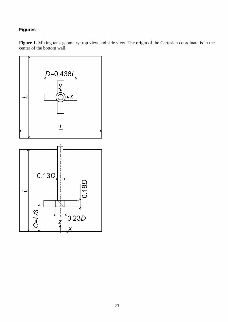
such that fluid is pumped downward. Figure 1 provides the geometrical details of the mixing tank. The
Reynolds number associated to the flow induced by the impeller is defined as 2Remx ND ν≡ with D the

6
impeller diameter and N the impeller speed (in revolutions per unit time). The flow systems contain a
Newtonian liquid with density ρ and kinematic viscosity ν and spherical solid particles of equal size
with diameter d and density sρ larger than ρ .
There are various ways to define the flow conditions in the systems as introduced above. The
dimensionless numbers we use to characterize the hindered settling systems are the average solids volume
fraction φ in the part of the volume loaded with particles, the density ratio sρ ρ , and the single-
particle settling Reynolds number Re u d ν∞ ∞≡ with u∞ the settling velocity that we determine from a
force balance over a single particle in an infinite domain ( ) 3 2 2126 4s Dg d C u dρ ρ π ρ π∞− = . For the drag
coefficient DC the Schiller-Naumann correlation [21] ( )0.68724 1 0.15Re ReDC = + is applied. For the
solid-liquid mixing simulations, next to the impeller-based Reynolds number Remx and the density ratio
sρ ρ there is the Shields parameter ( )2 2
s
N D
g d
ρθρ ρ
=−
. The latter expresses the competition between
inertial stress generated by the impeller motion suspending the particles (that scales with 2 2N Dρ ), and
net gravity pulling them down [6].
2.2 Liquid and solids dynamics
Fluid flow is solved on a three-dimensional Eulerian grid. The Eulerian grid is uniform and cubic with
grid spacing ∆ . The spherical particles that move through this grid have a diameter comparable to ∆ ; the
range of diameters investigated in this paper is 0.77 3.3d≤ ∆ ≤ . On the Eulerian grid the volume-
averaged continuity equation and momentum balance for the liquid phase [22,23] are solved:
( ) ( ) 0c c
tρφ ρφ∂ + ∇ ⋅ =
∂u (1)
( ) ( ) su uu π fc c c
tρφ ρφ φ∂ + ∇ ⋅ = ∇ ⋅ +
∂ (2)
7
with 1cφ φ≡ − the continuous phase (liquid) volume fraction and φ the solids volume fraction, u the
interstitial liquid velocity, π the liquid’s stress tensor, and sf the force per unit volume the solid particles
exert on the liquid. Equations 1 and 2 are solved with a variant of the lattice-Boltzmann method. Full
details can be found in [18,20].
The dynamics of the spherical solid particles is governed by Newton’s equations of motion
( )3 3
6 6p
h c x
uF F es s
dd d g
dt
π πρ ρ ρ= + − − (3)
5
60s
dd
dt
πρ = +ph c
ωT T (4)
and by
d
dt=p
p
xu (5)
with , ,p p pu ω x the linear velocity, angular velocity, and center location of a spherical particle
respectively (note that – because we are dealing with spheres – there is no need to track the angular
“location” of the particles), hF and hT the hydrodynamic force and torque on a particle, and cF and cT
the contact force and torque due to particle-particle collisions and lubrication effects.
2.3 Modelling assumptions and implementation
The only hydrodynamic force on the particles we will be considering is the drag force. For liquid-solid
systems – with density ratios of order one – additional hydrodynamic effects such as lift, added mass, and
history forces might have a significant effect [14]. At this stage we discard these effects. Eventually,
experimental data and sensitivity analyses through simulations will need to shed light on the importance
of additional forces under specific flow conditions.
The drag force is written in the form
( ) ( )3 Re,D pF u ud Fπρν φ= − (6)

8
with ( )Re 1 dφ ν= − − pu u .
An additional simplification thus is that drag only depends on the solids volume fraction, and on the
Reynolds number. That is, we do not include terms in the drag expression that depend on the granular
temperature (as in [12]), or on the Stokes number [11]. The function F is written as a product function
( ) ( ) ( )Re, ReF p qφ φ= . The Reynolds dependency is captured through the Schiller-Naumann correlation
[21] ( ) ( )0.687Re 1 0.15Rep = + (which is valid for Re 1,000< , a condition met in this paper). For the
dependence of drag on the local solids volume fraction we have tested two expressions: the Wen &Yu
expression ( ) ( )1qβφ φ −= − with 2.65β = [24] and the Van der Hoef et al expression
( ) ( ) ( ) ( )3 32
101 1
1q
φφ φ φφ
= + − +−
[25]. As has been noticed [11], the latter expression results in higher
values for the drag force as compared to the former. In [11] this has been identified as an effect of the
Stokes number. The Wen & Yu correlation has been derived from hindered settling experiments in solid-
liquid systems that have moderate Stokes numbers. The Van der Hoef et al expression is the result of
simulations of the flow around static, random assemblies of particles. This is a system characteristic for
infinite Stokes numbers. Since the solids are static and thus would take “infinite time” to change
configuration, the fluid phase time scales are infinitely smaller than those of the solids.
The force exerted by the fluid on the particle is the sum of DF and the contribution from a slowly
varying stress field (e.g. due to buoyancy) around the particle. This total hydrodynamic force on the
particle as it shows up in Eq. 3 can be expressed as ( )1h DF F φ= − [26]. One manifestation of a varying
stress field around the particles is the pressure that builds up as a consequence of the net weight of the
collection of particles. As will be shown, this results in a pressure gradient ( )m
pg
zρ ρ∂ = − −
∂ with
( )1m sρ φρ φ ρ= + − the mixture density. In this expression for the vertical pressure gradient, the liquid
density ρ is subtracted since Eq. 3 already accounts for the liquid-only buoyancy force.

9
The body force sf in Eq. 1 is the reaction of the drag force on the fluid. Feeding back the drag force
on the fluid is an example of mapping: relating Lagrangian properties (in this case drag force DF ) to
Eulerian properties (sf ).
The one-dimensional version of the mapping function used in this work reads
( )
( )
4 2
5 3
15 12 for
16
0 for
ξ ξµ ξ λ ξ λλ λ λ
µ ξ ξ λ
= − + − ≤ ≤
= > (7)
This is a “clipped fourth-order polynomial” [27] with λ the half-width of the mapping function. It shows
resemblance to a Gaussian distribution but is computationally more efficient to calculate than a Gaussian
and is zero at λ± . To determine some property α , that is known on the Eulerian grid, at a Lagrangian
location κ , the product of mapping function and property is integrated: ( ) ( ) ( )dλ
λ λα κ µ ξ κ α ξ ξ
−= −∫ .
The property ( )α ξ is defined on the equidistant Eulerian grid iξ with spacing ∆ by values iα . We
approximate ( )α ξ in the integrant as a stair-step function, i.e. ( ) iα ξ α= for 1 12 2i iξ ξ ξ− ∆ ≤ < + ∆ .
Given the discrete nature of ( )α ξ , the integral can be written as ( ) i iiλ
α κ η α= ∑ with iη coefficients
following from integrating the mapping function. The extension to a three-dimensional Eulerian grid and
a three dimensional Lagrangian location κ is straightforward and can be written as
( ) ijk ijki j kλ
α η α= ∑∑∑κ with , ,i j k discrete coordinates in x, y, and z-direction respectively. The
coefficients ijkη are only non-zero on grid points within a volume of ( )32λ around κ . Also 1ijk
i j kη =∑∑∑
since in case α is uniform, λα α= . For efficient calculations, we use a look-up table for determining
the coefficients ijkη . Prior to a simulation all coefficients ijkη are determined for a three-dimensional grid
of Lagrangian points (10×10×10 points in our code) in a grid cell. During the actual simulation, the
coefficients associated to a specific Lagrangian location (a particle) are obtained from tri-linear

10
interpolation in this grid of points. Interpolation guarantees smooth time-variation of the mapping
operations.
The coefficients ijkη are used to distribute Lagrangian properties to the grid. As an example, the
drag force on one of the particles (DF ) contributes to the body force on the fluid sf (see Eq. 2) in grid cell
, ,i j k by an amount 3
1ijkη−
∆ DF .
At three instances in the simulation procedure mapping operations are applied: (1) to determine the
liquid velocity u (to be used in Eq. 6 to determine the drag force) at the location of the particle from the
Eulerian velocity field; (2) to determine the Eulerian solids volume fraction field φ from the location and
size of the particles so that 1cφ φ= − is a known field when solving Eqs. 1 and 2; (3) (as explained
above) to determine the Eulerian vector field sf from the drag forces DF on the particles.
The choice of the width of the mapping function (λ ) is worthwhile investigating. Earlier research
[17,18] suggests a value of 1.5dλ = and we will be using this as our default choice. However, we will be
looking into the effects of excursions from this choice.
2.4 Particle dynamics
Equations 3 − 5 describe the dynamics of the particles. The way hF (in Eq. 3) has been determined was
shown above. The contact force cF consists of two parts: soft-sphere collision forces sscF and lubrication
forces lubF . Both forces are assumed to be radial forces. This means that they act on the line connecting
the two sphere centers involved in a contact. The collisions thus are assumed to be smooth so that we will
not be considering tangential contact forces and contact torques, as a result =cT 0 in Eq. 4.
The soft-sphere collision force is a radial repulsive force proportional to the distance δ over which
the spheres overlap: ( )2 2sscF cm tπ δ= with 3 6sm dπρ= the mass of a particle, and ct a parameter that
controls the typical time of contact between two particles [11]. Particle-wall collisions are treated similar
11
to particle-particle collisions: a fixed, fictitious particle is placed at the opposite side of the wall and the
actual particle bounces smoothly with the fictitious particle.
Lubrication forces occur when two closely spaced particles move relative to one another. The radial
component of the lubrication force (the only component considered here) is the result of a draining liquid
film between two approaching particles, and a liquid film filling upon separation. For low Reynolds
number film flow, the radial lubrication force on particle j due to particle i can be written as lub,j ijF nlubF=
with ( )ij p,j p,i p,j p,in x x x x= − − the unit vector along the line connecting the centers of the two particles,
and ( )238 p,j p,i iju u nlubF d sπνρ= − − ⋅ with s the minimum distance between particle surfaces [28]. The
force on particle i due to j is opposite: lub,i ijF nlubF= − . In the simulations these expressions have been
modified in two ways. (1) A cut-off distance of 0.1d has been introduced: for 0.1s d≥ the lubrication
force is zero, for 0.1s d< 1 10lubF s d∝ − [26]. (2) The lubrication force saturates if 310s d−≤ [26].
Since collisions between particles and between particles and walls are smooth, the only source of
rotation is the hydrodynamic torque hT (in Eq. 4). It is determined according to a creeping flow
approximation: ( )3 12dπρν= −h pT ω ω with ω the vorticity of the liquid in the direct vicinity of the
particle [29]. The hydrodynamic torque is not fed back to the liquid. As a result, the rotation of the
particles has no impact on the overall dynamics of the two-phase flow.
The equations of motion (Eq. 3-5) are solved by means of a split derivative time integration which
has been discussed in detail in [30]. Such integration enhances stability which is useful in case of modest
solid over liquid density ratios, as we have in this paper.
As a summary, we here list the main choices, assumptions and limitations of the proposed
simulation procedure: (a) Drag is the only hydrodynamic force; it depends on a particle-based Reynolds
number and local solids volume fraction. (b) Mapping functions with half-width 1.5dλ = are used to
relate Eulerian and Lagrangian flow properties; we will investigate the sensitivity with respect to dλ . (c)
Collisions are smooth, and interaction forces (soft-sphere and lubrication) are radial. (d) The torque on a
12
particle is estimated based on a creeping flow assumption and particle rotation is not fed back to the
liquid flow.
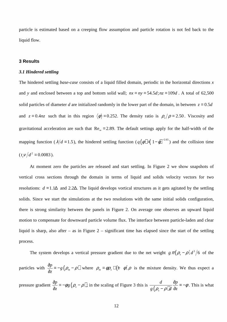
3 Results
3.1 Hindered settling
The hindered settling base-case consists of a liquid filled domain, periodic in the horizontal directions x
and y and enclosed between a top and bottom solid wall; 54.5 ; 109nx ny d nz d= = = . A total of 62,500
solid particles of diameter d are initialized randomly in the lower part of the domain, in between 0.5z d=
and 0.4z nz= such that in this region φ = 0.252. The density ratio is 2.50sρ ρ = . Viscosity and
gravitational acceleration are such that Re∞ = 2.89. The default settings apply for the half-width of the
mapping function ( 1.5dλ = ), the hindered settling function (( ) ( ) 2.651q φ φ −= − ) and the collision time
( 2 0.0083ct dν = ).
At moment zero the particles are released and start settling. In Figure 2 we show snapshots of
vertical cross sections through the domain in terms of liquid and solids velocity vectors for two
resolutions: 1.1d = ∆ and 2.2∆. The liquid develops vortical structures as it gets agitated by the settling
solids. Since we start the simulations at the two resolutions with the same initial solids configuration,
there is strong similarity between the panels in Figure 2. On average one observes an upward liquid
motion to compensate for downward particle volume flux. The interface between particle-laden and clear
liquid is sharp, also after – as in Figure 2 – significant time has elapsed since the start of the settling
process.
The system develops a vertical pressure gradient due to the net weight ( ) 3 6sg dπ ρ ρ− of the
particles with ( )m
pg
zρ ρ∂ = − −
∂ where ( )1m sρ φρ φ ρ= + − is the mixture density. We thus expect a
pressure gradient ( )s
pg
zφ ρ ρ∂ = − −
∂; in the scaling of Figure 3 this is ( )s
d p
g d zφ
ρ ρ∂ = −
− ∂. This is what

13
is observed in the left panel of Figure 3: the slope of the pressure profile in the part of the volume that
contains settling particles is approximately 0.25− which is minus the average solids volume fraction φ
there. The solids volume fraction contours in Figure 3 are consistent with the pressure profile:
approximately zero pressure gradient in the clear liquid and in the settled granular bed on the bottom wall,
and a constant, negative gradient in the region where the particles settle.
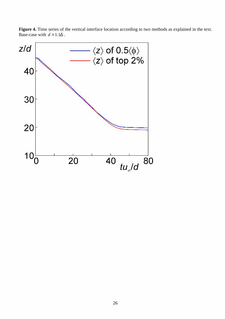
Hindered settling speeds have been determined as it would have been done in an experiment:
measure the vertical location of the interface between suspension and clear liquid as a function of time.
As we observed in Figures 2 and 3, the interface is well-defined and horizontal. Two different ways of
quantifying the interface location have been tested: (1) the laterally (x and y) averaged z location where
the Eulerian solids volume fraction field is half the solids volume fraction in the suspension; (2) the
average z location of the top 2% of the particles. In Figure 4 it shows that the results of two methods have
close resemblance. The settling speeds as presented in the remainder of this section have been determined
with the second (top 2%) method by fitting a straight line to the linear portion of the time series as this
method shows a slightly smoother time series (see Figure 4).
In Figure 5 it is demonstrated that the simulation procedure mimics the dependency of the settling
velocity on the average solids volume fraction as proposed by Richardson & Zaki [2] quite well (left
panel of Figure 5). In a more critical test we compare hindered settling in terms of the exponent n in the
settling function ( ( )1n
su u φ∞ = − ) and the way it depends on a Reynolds number su d ν with an
empirical correlation due to Di Felice [31]. The simulations show an n that is some 10% lower than the
empirical correlation. The weakly downward trend in n with respect to the Reynolds number is
represented correctly by the simulations.
In our previous work [18] it was shown that average slip velocities were virtually insensitive for the
half-width of the mapping function λ as long as 1.5dλ ≥ . The left panel of Figure 6 confirms this for
the current hindered settling simulations. More importantly, however, the spatial resolution of the
simulations expressed as d ∆ at fixed 1.5dλ = has virtually no effect on the settling velocity (see the

14
right panel of Figure 6). It implies that – at least for average settling speeds – there is freedom in choosing
spatial resolution relative to the particle size, at least in the range 1 3d≤ ∆ ≤ . The situation for
fluctuating velocities is more complicated in the case of the present simulations. Where the settling speed
is steady in a significant part of the time window of a simulation (see Figure 4), the per-particle variability
in the velocity (expressed in a root-mean-square value) is a transient as shown in Figure 7. The root-
mean-square (rms) values are – as expected – larger for the vertical velocity component than for the
horizontal components (by approximately a factor of 2) [20,32]. The dependency of the rms particle
velocity values with respect to the width of the mapping function follow the same trend as in the (fully
periodic) simulations in [18]: the wider the mapping function, the weaker the rms velocity values (in [18]
it was argued that for dλ → ∞ fluctuations would disappear). From comparison with particle-resolved
simulations, 1.5dλ = was found to be the mapping function width that best mimicked the particle
resolved simulations [18], in line with conclusions drawn in [17]. With the latter value for dλ the
sensitivity of the rms velocities with respect to d ∆ was assessed, see the right panel of Figure 7. The
outlier in this panel is the simulation with the lowest resolution (at d ∆ =0.77). As long as 1.1d ∆ ≥ , the
resolution of the particles on the grid has no significant impact on the rms particles velocity values.
In summary, the mapping procedure, in combination with the lattice-Boltzmann based numerical
scheme, shows for hindered settling towards a solid wall results that are largely independent on the level
of resolution of the particles on the grid, as expressed through the ratio of particle size and grid spacing
d ∆ . It is important to realize that the most appropriate choice of 1.5dλ = is based on a limited range of
solids volume fractions and (particle-based) Reynolds numbers. It might very well be – and some of the
comparisons with particle resolved simulations as presented in [18] indeed suggest so – that the choice of
1.5dλ = is regime dependent. In the subsequent section, the numerical procedure will be applied to a
mixing tank configuration where, next to determining particle dynamics, also resolving the complex flow
generated by the impeller imposes demands on the grid spacing.

15
3.2 Agitated solid-liquid flow
The dimensionless numbers we use for defining the agitated flow in the mixing tank (with geometry and
aspect ratios as given in Figure 1) have values 2Remx ND ν≡ =4,000, ( )2 2
s
N D
g d
ρθρ ρ
=−
=260, and
sρ ρ =2.23. The particle size relative to the impeller diameter is d D =0.0208; the tank-averaged solids
volume fraction, i.e. total volume of solids over total tank volume is φ =0.098; the number of particles
is 250,000. A Stokes number with ( )1 4N (the inverse of the impeller blade passage frequency) is
defined as 2
29
4St s d Nρ
ρ ν≡ and has value of 3.4, i.e. an intermediate Stokes number.
The main purpose of this study of agitated solid-liquid flow is to establish grid independence.
Sufficiently fine grids are required to resolve the flow at the given − impeller-based − Reynolds number.
The settling simulations have shown that, with the proposed mapping procedure, there is freedom in the
choice of the particle diameter relative to the grid spacing. In the right panels of Figure 6 and 7 it is
shown that results on respectively settling speed and particle velocity fluctuations during settling are not
sensitive to the particle size relative to the grid spacing as long as 1.1d ∆ ≥ . Four levels of resolution
have been applied to the agitated flow system: d ∆ =1.0, 1.6, 2.0, 2.5 with all four simulations having the
same physical dimensionless parameters given above. The coarsest grid consists of 1103 cubic cells, the
finest of 2753. Expressed in terms of lattice spacings per impeller diameter, the four resolutions are
D ∆ = 48, 76.8, 96, and 120 respectively.
The initial conditions for each simulation are the same: an initial particle configuration is created by
letting the 250,000 particles (with d ∆ =1.0) settle in a cubic container. Each of the four simulations uses
exactly the same dense layer of particles resting on the bottom of the tank with the (x,y,z) locations of the
particles scaled according to the specific resolution of the simulation. At moment t=0, when fluid and
particles have zero velocity, the impeller is set to rotate. The impeller speed is ramped up to its steady

16
state value N such that the first impeller revolution takes a time of2 N ; beyond 2t N= the impeller
spins at constant speed N.
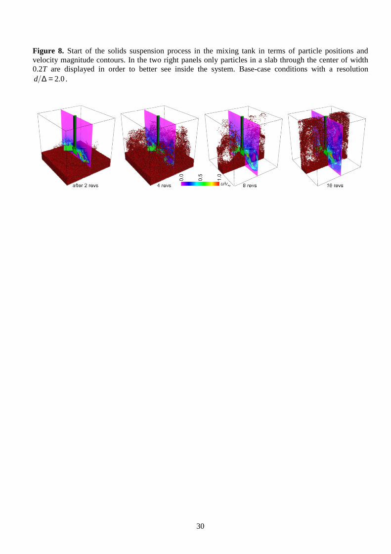
For illustration, we show snapshots of the start-up of the suspension process for the simulation with
d ∆ =2.0 in Figure 8. The velocity magnitude contours in a vertical plane through the center of the tank
show liquid being pumped by the impeller in a downward-radial direction. This stream agitates the
particles that – as a result – get suspended. Some particles reach the top of the tank within the time needed
for eight impeller revolutions. After 16 revolutions particles can be found throughout the entire tank
volume, although their distribution is clearly inhomogeneous.
Before discussing the way particles distribute over the tank volume, first the effects of grid
resolution on the liquid flow predictions will be discussed. In Figure 9 we show snapshots of the flow
close to an impeller blade taken at the same number of impeller revolutions after startup for two different
spatial resolutions in terms of liquid and particle velocity vectors. That the overall flow patterns in the
two panels of Figure 9 are different is not a direct concern: The impeller generates a mildly turbulent (or
transitional) flow so that we expect randomness in the temporal variability of the flow. The left, more
resolved panel, however, shows much more fine, small scale detail that seems to be too small to be
captured on the coarser grid in the right panel, for example the vortex underneath the hub. We thus
anticipate the latter simulation (with 48D = ∆ ) to be under-resolved.
We realize (1) that these are only qualitative observations, and (2) that it might very well be that the
simulation in the left panel is under-resolved as well. In fact, in order to fully resolve boundary layers on
impeller blades at the current Reynolds number, linear mesh spacings might need to be smaller by an
order of magnitude. The boundary layers are, however, not critical for the bulk flow in the tank [33]; the
bulk flow is where the main solid-liquid interactions take place.
As a more objective, albeit global, measure for grid convergence the torque M required to spin the
impeller is compared between the various grids. If we define the dimensionless torque as
( )2 5Po 2 M N Dπ ρ= it is equivalent to the power number (since power 2P NMπ= ). Time series of Po

17
are shown in Figure 10. They show some time variability as well as a strong effect of the spatial
resolution of the simulations. For all cases, a quasi steady state is reached after approximately 20 impeller
revolutions. The figure indicates that grid convergence is reached if in the simulation the resolution is
such that 96D ∆ ≥ (equivalent to 2.0d ∆ ≥ ). This is an important result. It teaches that the required
resolution is in the first place dictated by the liquid flow dynamics. If particles are involved in the flow,
we thus need the freedom to choose their size independent of the grid spacing. The results on sedimenting
systems in the previous section suggest that with the current mapping procedure particle size
independence can be achieved. In the remainder of this paper we will test particle size independence for
the more complicated situation (as compared to simple, hindered settling) of a mildly turbulent agitated
flow.
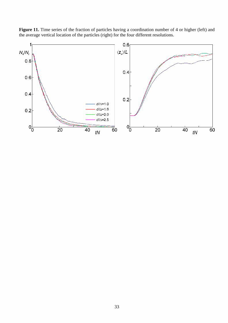
Time series of two global particle characteristics are compared for the four resolutions in Figure 11.
The left panel shows the number of particles with coordination number of at least 4 (4N ) over the total
number of particles ( tN ). The coordination number of a particle is the number of other particles it is in
contact with, where contact is defined as overlap 0δ > . Since we start from a dense granular bed on the
bottom of the tank, the ratio 4 tN N is close to one at time zero, and in the subsequent suspension process
the ratio 4 tN N gets reduced. The fact that it gets reduced to close to zero implies that the solids
suspension process under the conditions considered approaches complete suspension over the 60 impeller
revolutions of the time series. The second global particle characteristic is the average vertical (z) particle
location, plotted as a function of time in the right panel of Figure 11. Both time series show a significant
difference between on one side the simulation with 1d ∆ = , and on the other side the other three
simulations. This is consistent with the results for the power number (Figure 10) where also the 1d ∆ =
stood out from the others. The difference as observed in power number for 1.6d ∆ = with the finer
simulations, however, does not reflect in markedly different global particle behavior.

18
In Figures 12 and 13 a more local characterization of the suspension process is presented. Here we
look into what happens around time 20tN = . Considering this moment in time when the suspension
process is still in progress (see Figure 11) is a more interesting and critical test for assessing resolution
effects than looking at the fully suspended, quasi steady state. Figure 12 shows instantaneous realizations
at 20tN = of the situation in a vertical cross section through the center of the tank for the four
simulations considered. The way individual particles intersect that plane is indicated by the white disks;
the colors indicate the instantaneous Eulerian solids volume fraction fields as obtained through mapping
from the particle locations and the figure thus serves as an illustration of how the mapping operation
works. The particles concentrate under the impeller since the flow there is relatively weak (see Figure 9).
There are more particles close to the bottom for the least resolved simulation ( 1d ∆ = ) compared to the
other simulations, in line with the results in Figure 12. No systematic differences between the other
simulations can be concluded from the snapshots in Figure 12. For this reason average solids volume
fraction fields over the period 15 20tN≤ ≤ are shown in Figure 13. They confirm the least level of solids
suspension for 1d ∆ = and tentatively – not significantly – show less particles in the bottom region and
in the solids cone underneath the impeller the higher the spatial resolution of a simulation. We conclude
from these results that a decent level of grid independence for this two-phase system under its current
conditions is achieved for 2d ∆ ≥ .
It should be realized that the primary purpose of this paper is to establish a procedure for solid-
liquid simulations in which the resolution can be tailored independently to the needs of fluid as well as
solids mechanics. The level of realism of the simulation results depends on much more than on (the
elimination of) grid effects only. One of the choices we made was for the Wen & Yu drag force
correlation [24]; another choice was the incorporation of lubrication forces. To judge the impact of these
specific choices, two additional simulations (with resolution 1.6d ∆ = ) were performed. One using the
Van der Hoef et al drag force expression [25] instead of the Wen & Yu correlation, the other without

19
lubrication forces. Results are in Figure 14. They have been presented in the same way as the results in
Figures 12 and 13 for the base-cases.
The effects of the lubrication force are very significant: suspending the solids is much easier
without activated lubrication forces. Mobilizing the granular bed requires pulling apart connected
particles. In this process the lubrication force is an attractive force. The change in drag correlation is less
drastic but still visible: suspension of the solids after 20 impeller revolutions has advanced less with the
Van der Hoef et al correlation as compared to the Wen & Yu correlation.
5 Conclusions and outlook
In this paper we have assessed a procedure – based on the lattice-Boltzmann method – for performing
Eulerian-Lagrangian simulations of dense solid-liquid systems with unresolved particles. We focused on
the effects of spatial resolution. Two flow systems were considered: (1) settling of particles under gravity
towards a solid, horizontal wall; (2) an agitated tank with particles getting suspended by a transitional
(Reynolds number 4,000) liquid flow. The modelling approach is relatively simple: drag and lubrication
are the only hydrodynamic forces considered. The drag force depends on the local solids volume fraction
through the Wen & Yu correlation [24] which we justify because we are dealing with solid-liquid systems
(that have modest Stokes numbers). Particle collisions are smooth. The solids and liquid dynamics are
two-way coupled except for particle rotation which is one-way (only fluid to solid) coupled.
The main conclusion of the sedimentation simulations is that the results in terms of average settling
speed as well as particle velocity fluctuations are independent of the particle size relative to the lattice
spacing if we use mapping functions with a fixed width relative to the particle size. The dependency of
the hindered settling speed as a function of the average solids volume fraction is in reasonable agreement
with empirical correlations from the literature [31].
The independence of the particle size relative to the grid spacing is an important feature if the grid
resolution is decided by factors other than the solids dynamics. In the case of the mixing tank, the

20
transitional flow generated by the impeller is decisive for the choice of resolution and grid effects first
and foremost show up for the torque required to spin the impeller. Global and local parameters
characterizing the solids suspension process showed grid-independent behavior beyond a certain spatial
resolution. It should be realized that simulation results – including those that approach grid-independence
– depend on the choice of the width of the mapping function relative to the particle size. Further study is
needed to explore how to objectively make this choice and to what extent this choice is regime (solids
volume fraction, Reynolds number, Stokes number) dependent.
Given the relative simplicity of the way solids dynamics has been modelled and coupled to the
liquid dynamics there is ample room for model refinement. An important question in this respect is,
however, how to judge if model refinement leads to improvement of the level of realism of the
simulations. In our opinion we need detailed experiments for this, e.g. based on visualization and optical
velocity measurements in refractive index matched solid-liquid systems [19]. For example, an experiment
along these lines in a mixing tank would be able to decide if the role of the lubrication force is indeed as
important as shown by the numerical results in this paper, or if there are advantages of using one
formulation of a drag force correlation over another.

21
References
[1] Stokes GG. Mathematical and Physical Papers, Volumes I-V. Cambridge: Cambridge University
Press; 1901.
[2] Richardson JF, Zaki WN. Sedimentation and fluidisation. Part 1. Trans. Inst. Chem. Engrs. 1954; 32:
35–53.
[3] Zwietering ThN. Suspending of solid particles in liquid by agitators. Chem. Engng. Sc. 1958; 9, 244–
253.
[4] Uhlmann M. Interface-resolved direct numerical simulation of vertical particulate channel flow in the
turbulent regime. Phys. Fluids 2008; 20: 053305.
[5] Lucci F, Ferrante A, Elghobashi S. Modulation of isotropic turbulence by particles of Taylor length-
scale size. J. Fluid Mech. 2010; 650: 5–55.
[6] Derksen JJ. Highly resolved simulations of solids suspension in a small mixing tank. AIChE J. 2012;
58: 3266–3278.
[7] Wachs A, Hammouti A, Vinay G, Rahmani M. Accuracy of finite volume/staggered grid distributed
Lagrange multiplier/fictitious domain simulations of particulate flows. Comp. Fluids 2015; 115:
154–172.
[8] Kidanemariam, A.G., Uhlmann, M. Formation of sediment patterns in channel flow: minimal
unstable systems and their temporal evolution. J. Fluid Mech. 2017; 818: 716–743.
[9] Beetstra R, Van der Hoef MA, Kuipers JAM. Drag force of intermediate Reynolds number flow past
mono- and bi-disperse arrays of spheres. AIChE J. 2007; 52: 489–501.
[10] Tenneti S, Garg R, Subramaniam S. Drag law for monodisperse gas–solid systems using particle-
resolved direct numerical simulation of flow past fixed assemblies of spheres. Int. J. Multiphase
Flow 2011; 37: 1072–1092.
[11] Rubinstein GJ, Derksen JJ, Sundaresan S. Lattice-Boltzmann simulations of low-Reynolds number
flow past fluidized spheres: effect of Stokes number on drag force. J. Fluid Mech. 2016; 788: 576–
601.
[12] Wylie JJ, Koch DL, Ladd AJC. Rheology of suspensions with high particle inertia and moderate fluid
inertia. J. Fluid Mech. 2003; 480: 95–118.
[13] Clift R, Grace JR, Weber ME. Bubbles, Drops, and Particles. New York: Academic Press; 1978.
[14] Maxey MR, Riley JJ. Equation of motion for a small rigid sphere in a nonuniform flow. Phys. Fluids
1983; 26: 883–889.
[15] Deen NG, Van Sint Annaland M, Van der Hoef MA, Kuipers JAM. Review of discrete particle
modeling of fluidized beds. Chem. Eng. Sc. 2007; 62: 28–44.
22
[16] Derksen JJ. Numerical simulation of solids suspension in a stirred tank. AIChE J. 2003; 49: 2700–
2714.
[17] Capecelatro J, Desjardins O. An Euler–Lagrange strategy for simulating particle-laden flow., J.
Comp. Phys. 2013; 238: 1–31.
[18] Derksen JJ. Assessing Eulerian-Lagrangian simulations of dense solid-liquid suspensions settling
under gravity. Comp. & Fluids 2016 in press; http://dx.doi.org/10.1016/j.compfluid.2016.12.017.
[19] Genghong Li, Zhengming Gao, Zhipeng Li, Jiawei Wang, Derksen JJ. Particle-resolved PIV
experiments of solid-liquid mixing in a turbulent stirred tank. AIChE J. 2017; under review.
[20] Sungkorn R, Derksen JJ. Simulations of dilute sedimenting suspensions at finite-particle Reynolds
numbers. Phys. Fluids 2012; 24: 123303.
[21] Schiller L, Naumann A. Uber die grundlagenden Berechnungen bei der Schwerkraftaufbereitung.
Ver. Deut. Ing. Z. 1933; 77: 318–320.
[22] Sankaranarayanan K, Sundaresan S. Lattice Boltzmann simulation of two-fluid model equations. Ind.
Eng. Chem. Res. 2008; 47: 9165–9173.
[23] Gidaspow D. Multiphase Flow and Fluidization. San Diego: Academic Press: 1994.
[24] Wen CY, Yu YH. Mechanics of fluidization. Chem. Engng. Prog. 1966; 62; 100–111.
[25] Van der Hoef MA, Beetstra R, Kuipers JAM. Lattice-Boltzmann simulations of low-Reynolds-
number flow past mono- and bidisperse arrays of spheres: results for the permeability and drag
force. J. Fluid Mech. 2005; 528, 233-254.
[26] Derksen JJ, Sundaresan S. Direct numerical simulations of dense suspensions: wave instabilities in
liquid-fluidized beds. J. Fluid Mech. 2007; 587: 303–336.
[27] Deen NG, Van Sint Annaland M, Kuipers JAM. Multi-scale modeling of dispersed gas–liquid two-
phase flow. Chem. Eng. Sc. 2004; 59: 1853–1861.
[28] Kim S, Karrila SJ. Microhydrodynamics: Principles and selected applications. Boston: Butterworth-
Heinemann; 1991.
[29] Deen WM. Analysis of transport phenomena. New York: Oxford University Press; 1998.
[30] Shardt O, Derksen JJ. Direct simulations of dense suspensions of non-spherical particles. Int. J.
Multiphase Flow 2012; 47: 25–36.
[31] Di Felice R. The voidage function for fluid-particle interaction systems. Int. J. Multiphase Flow.
1994; 20: 153–159.
[32] Guazzelli É, Hinch J. Fluctuations and instability in sedimentation. Annu. Rev. Fluid Mech. 2011;
43: 97–116.
[33] Derksen J, Van den Akker HEA. Large-eddy simulations on the flow driven by a Rushton turbine.
AIChE J. 1999; 45: 209–221.
23
Figures
Figure 1. Mixing tank geometry: top view and side view. The origin of the Cartesian coordinate is in the center of the bottom wall.

24
Figure 2. Base-case for hindered settling at two resolutions: left 1.1d = ∆ , right 2.2d = ∆ . Instantaneous realizations 13.4tu d∞ = after start-up. Cross sections through the middle of the flow domain. Black
vectors: interstitial liquid velocity; red vectors: velocity of particles in a 4d thick layer in the middle of the domain. The reference vector indicates the single-particle settling velocity u∞ .

25
Figure 3. Left: the solid blue curve is the vertical pressure profile averaged over the lateral directions p ; the dashed line is to show slope 0.25− . Right: solids volume fraction distribution in a vertical cross
section. Instantaneous realization at 35.9tu d∞ = . Base-case with 1.1d = ∆ .
26
Figure 4. Time series of the vertical interface location according to two methods as explained in the text. Base-case with 1.1d = ∆ .

27
Figure 5. Left: hindered settling velocity as a function of solids volume fraction for Re∞ = 2.89,
2.50sρ ρ = , 1.1d ∆ = , and 1.5dλ = . Right: same data as in left figure with ln1
su un
φ∞
= −
; the curve
is ( )24.7 0.65exp 1.5 2n x = − − −
with ( )10 log sx u d ν= due to Di Felice [30].

28
Figure 6. Settling speed as a function of numerical parameters. Left: effect of the half-width of the mapping function (λ ) for 1.1d = ∆ . Right: effect of particle size relative to grid spacing (d ∆ ) for
1.5dλ = . In all cases, Re∞ = 2.89, 2.50sρ ρ = ; φ as indicated.

29
Figure 7. Time series of particle velocities fluctuation levels (root-mean-square values) in horizontal and vertical direction in a horizontal layer with thickness 8d centered at 3z nz= . Left: effect of λ for
1.1d = ∆ . Right: effect of d with 1.5dλ = . Re∞ = 2.89, 2.50sρ ρ = ; φ =0.252.
30
Figure 8. Start of the solids suspension process in the mixing tank in terms of particle positions and velocity magnitude contours. In the two right panels only particles in a slab through the center of width 0.2T are displayed in order to better see inside the system. Base-case conditions with a resolution
2.0d ∆ = .

31
Figure 9. Impressions of instantaneous flow near the impeller (area indicated in grey in the right panel). Black vectors are liquid velocity, red vectors particle velocity. The blue dots are the points used in the immersed boundary method to represent the impeller. The left panel ( 2.0d ∆ = ) has a twice as high
resolution as the middle panel ( 1.0d ∆ = ). Base-case conditions; 29 impeller revolutions after start-up.

32
Figure 10. Left: time series of power number Po for simulations with different resolution; right: time-averaged power number determined for 20tN ≥ .
33
Figure 11. Time series of the fraction of particles having a coordination number of 4 or higher (left) and the average vertical location of the particles (right) for the four different resolutions.

34
Figure 12. Instantaneous realizations of the solids volume fraction in a vertical plane through the center of the tank at 20tN = . The white dots are cross sections of individual particles. Increasing resolution from left to right: d ∆ = 1.0, 1.6, 2.0, and 2.5 respectively.

35
Figure 13. Time-averaged solids volume fraction in a vertical plane through the center of the tank. Averaging over five impeller revolutions 15 20tN≤ ≤ . Increasing resolution from left to right: d ∆ = 1.0, 1.6, 2.0, and 2.5 respectively.

36
Figure 14. Top row: instantaneous realizations of the solids volume fraction in a vertical plane through the center of the tank at 20tN = ; bottom row: time-averaged (15 20tN≤ ≤ ) solids volume fraction. Left: Van der Hoef et al [24] instead of Wen & Yu drag correlation; right: lubrication force switched off. In both cases d ∆ = 1.6


