Embed Size (px)
Citation preview
Quantum manipulation of nitrogen-vacancy centersin diamond: from basic properties to applications
A dissertation presented
by
Jeronimo Maze Rios
to
The Department of Physics
in partial fulfillment of the requirements
for the degree of
Doctor of Philosophy
in the subject of
Physics
Harvard University
Cambridge, Massachusetts
April 2010

c©2010 - Jeronimo Maze Rios
All rights reserved.
Thesis advisor Author
Mikhail D. Lukin Jeronimo Maze Rios
Quantum manipulation of nitrogen-vacancy centers in
diamond: from basic properties to applications
Abstract
This thesis presents works not only to understand the spin degree of freedom
present in the nitrogen-vacancy defect in diamond: its internal structure and its re-
lation to its environment, but also to find novel applications of it in metrology. First,
a mathematical model is develop to understand how this defect couples to a nuclear
spin bath of Carbon 13 which constitutes the main dephasing mechanism in pure
natural diamond. Next, we demonstrate the use of this defect to sense external os-
cillating magnetic fields. The high sensitivity and the small sensing volume achieved
when a defect is placed in a nanocrystal of few tents of nanometers in diameter, al-
lows this sensor to detect single electronic spins and even single nuclear spins. This
sensitivity, proportional to the signal to noise per readout, can be improve by the help
of the environment of this defect. We show that strongly interacting nearby nuclei
can enable repetitive readout schemes to improve the signal to noise of the electronic
spin signal. We also combine ideas from the microscopy community such as stimu-
lated emission depletion to enable high spatial resolution magnetometry. Finally, we
develop a formalism based on group theory to understand the internal structure of
defects in solids such as their selection rules and the effect of spin-spin and spin-orbit
iii

Abstract iv
interactions even when perturbations reduce the symmetry group of the system.

Contents
Title Page . . . . . . . . . . . . . . . . . . . . . . . . . . . . . . . . . . . . iAbstract . . . . . . . . . . . . . . . . . . . . . . . . . . . . . . . . . . . . . iiiTable of Contents . . . . . . . . . . . . . . . . . . . . . . . . . . . . . . . . vCitations to Previously Published Work . . . . . . . . . . . . . . . . . . . viiiAcknowledgments . . . . . . . . . . . . . . . . . . . . . . . . . . . . . . . . ixDedication . . . . . . . . . . . . . . . . . . . . . . . . . . . . . . . . . . . . xiii
1 Introduction 11.1 Background . . . . . . . . . . . . . . . . . . . . . . . . . . . . . . . . 11.2 Description of this thesis . . . . . . . . . . . . . . . . . . . . . . . . . 3
1.2.1 Decoherence . . . . . . . . . . . . . . . . . . . . . . . . . . . . 41.2.2 Applications . . . . . . . . . . . . . . . . . . . . . . . . . . . . 51.2.3 Understanding defects . . . . . . . . . . . . . . . . . . . . . . 7
2 Decoherence of single electronic spin in diamond 92.1 Introduction . . . . . . . . . . . . . . . . . . . . . . . . . . . . . . . . 9
2.1.1 System and Spin hamiltonian . . . . . . . . . . . . . . . . . . 112.2 Method: Disjoint cluster approach . . . . . . . . . . . . . . . . . . . . 132.3 Electron spin-echo . . . . . . . . . . . . . . . . . . . . . . . . . . . . 15
2.3.1 Non-interacting bath . . . . . . . . . . . . . . . . . . . . . . . 172.3.2 Interacting bath: an example . . . . . . . . . . . . . . . . . . 18
2.4 Application of the disjoint cluster approach . . . . . . . . . . . . . . . 192.4.1 Grouping algorithm . . . . . . . . . . . . . . . . . . . . . . . . 202.4.2 Numerical methods and example cases . . . . . . . . . . . . . 21
2.5 Results and Discussion . . . . . . . . . . . . . . . . . . . . . . . . . . 232.6 Comparison with experiments . . . . . . . . . . . . . . . . . . . . . . 30
2.6.1 Ensemble measurements . . . . . . . . . . . . . . . . . . . . . 312.7 Conclusions . . . . . . . . . . . . . . . . . . . . . . . . . . . . . . . . 32
3 Magnetic field sensing with an individual electronic spin in diamond 343.1 Introduction . . . . . . . . . . . . . . . . . . . . . . . . . . . . . . . . 34
v

Contents vi
3.2 Implementation of spin-based magnetometry using NV centers . . . . 383.3 Magnetic sensing using diamond nanocrystals . . . . . . . . . . . . . 443.4 Outlook and Conclusions . . . . . . . . . . . . . . . . . . . . . . . . . 46
4 Repetitive readout of a single electronic spin via quantum logic withnuclear spin ancillae 474.1 Introduction . . . . . . . . . . . . . . . . . . . . . . . . . . . . . . . . 474.2 Repetitive readout scheme . . . . . . . . . . . . . . . . . . . . . . . . 484.3 Implementation with nearby 13C ancillae . . . . . . . . . . . . . . . . 504.4 Outlook and Conclusions . . . . . . . . . . . . . . . . . . . . . . . . . 61
5 Imaging and manipulation of individual spins with nanoscale reso-lution 635.1 Introduction . . . . . . . . . . . . . . . . . . . . . . . . . . . . . . . . 635.2 Breaking the diffraction limit resolution . . . . . . . . . . . . . . . . 665.3 High resolution spin imaging and magnetometry . . . . . . . . . . . . 715.4 Coherent manipulation by inhibiting spin transitions . . . . . . . . . 725.5 Outlook and Conclusions . . . . . . . . . . . . . . . . . . . . . . . . . 75
6 Group theoretical description of the nitrogen-vacancy center in di-amond 776.1 Introduction . . . . . . . . . . . . . . . . . . . . . . . . . . . . . . . . 776.2 State representation . . . . . . . . . . . . . . . . . . . . . . . . . . . . 806.3 Ordering of singlet states . . . . . . . . . . . . . . . . . . . . . . . . . 846.4 Spin-Orbit interaction . . . . . . . . . . . . . . . . . . . . . . . . . . 876.5 Spin-spin interaction . . . . . . . . . . . . . . . . . . . . . . . . . . . 906.6 Selection rules and spin-photon entanglement schemes . . . . . . . . . 936.7 Effect of strain . . . . . . . . . . . . . . . . . . . . . . . . . . . . . . 95
6.7.1 Strain and Electric field . . . . . . . . . . . . . . . . . . . . . 1016.8 Conclusions . . . . . . . . . . . . . . . . . . . . . . . . . . . . . . . . 104
7 Conclusions and Outlook 105
A Supporting material for Chapter 2 109A.1 Phenomenological models for decoherence . . . . . . . . . . . . . . . 109A.2 Decoherence due to off-axis magnetic field . . . . . . . . . . . . . . . 112A.3 Ensemble measurements . . . . . . . . . . . . . . . . . . . . . . . . . 113A.4 Non-Secular Correction . . . . . . . . . . . . . . . . . . . . . . . . . . 114
B Supporting material for Chapter 3 123B.1 Samples . . . . . . . . . . . . . . . . . . . . . . . . . . . . . . . . . . 123B.2 Confocal Setup . . . . . . . . . . . . . . . . . . . . . . . . . . . . . . 123B.3 Single Center Electron Spin Resonance . . . . . . . . . . . . . . . . . 127
Contents vii
B.4 AC magnetometry . . . . . . . . . . . . . . . . . . . . . . . . . . . . 128
C Supporting material for Chapter 4 131C.1 Experimental Setup . . . . . . . . . . . . . . . . . . . . . . . . . . . . 131C.2 Effective Hamiltonian . . . . . . . . . . . . . . . . . . . . . . . . . . . 137C.3 Nuclear Spin Depolarization for Each Readout . . . . . . . . . . . . . 146C.4 Deriving Optimized SNR . . . . . . . . . . . . . . . . . . . . . . . . . 147C.5 Simulation for the Repetitive Readout . . . . . . . . . . . . . . . . . 150
D Supporting material for Chapter 5 154D.1 Irradiation and annealing procedure . . . . . . . . . . . . . . . . . . . 154D.2 Confocal and spin-RESOLFT microscopy . . . . . . . . . . . . . . . . 155D.3 Generation of Doughnut beam . . . . . . . . . . . . . . . . . . . . . . 155D.4 Spin imaging resolution . . . . . . . . . . . . . . . . . . . . . . . . . . 157D.5 Measurements of local magnetic field environment with sub-diffraction
resolution . . . . . . . . . . . . . . . . . . . . . . . . . . . . . . . . . 160D.6 Inhibition of Electron-Spin Rabi Oscillations via Quantum Zeno-like
Effect . . . . . . . . . . . . . . . . . . . . . . . . . . . . . . . . . . . 164
E Supporting material for Chapter 6 170E.1 Dangling bond representation and character table . . . . . . . . . . . 170E.2 Ordering of singlet states . . . . . . . . . . . . . . . . . . . . . . . . . 173E.3 Spin-spin interaction . . . . . . . . . . . . . . . . . . . . . . . . . . . 174E.4 Strain and electric field . . . . . . . . . . . . . . . . . . . . . . . . . . 176E.5 Information about the first principles methods applied in our study . 178
Bibliography 180

Citations to Previously Published Work
Large portions of Chapter 2 have appeared in the following paper:
“Electron spin decoherence of single nitrogen-vacancy defects in diamond”,J. R. Maze, J. M. Taylor, and M. D. Lukin, Phys. Rev. B 78, 094303(2008), abs/0805.0327.
Chapter 3 appeared in the following publication:
“Nanoscale magnetic sensing with an individual electronic spin in dia-mond”, J. R. Maze, P. L. Stanwix, J. S. Hodges, S. Hong, J. M. Taylor,P. Cappellaro, L. Jiang, M. V. Gurudev Dutt, E. Togan, A. S. Zibrov, A.Yacoby, R. L. Walsworth and M. D. Lukin, Nature 455, 644-647 (2008).
Chapter 4 appears in its entirety as
“Repetitive Readout of a Single Electronic Spin via Quantum Logic withNuclear Spin Ancillae”, L. Jiang, J. S. Hodges, J. R. Maze, P. Maurer, J.M. Taylor, D. G. Cory, P. R. Hemmer, R. L. Walsworth, A. Yacoby, A. S.Zibrov and M. D. Lukin, Science 326, 267 (2009).
Most of Chapter 5 has been published as
“Far-field optical imaging and manipulation of individual spins with nanoscaleresolution”, P. C. Maurer, J. R. Maze, P. L. Stanwix, L. Jiang, A.V. Gor-shkov, A.A. Zibrov, B. Harke, J.S. Hodges, A.S. Zibrov, D. Twitchen,S.W. Hell, R.L. Walsworth, and M.D. Lukin, submitted to Nature Physics(2009).
Finally, some portions of Chapter 6 is in preparation and it will be published as
“Group theory of defects: Nitrogen vacancy center in diamond”, J. R.Maze, A. Gali, E. Togan, Y. Chu, A. Trifonov, E. Kaxiras, and M. D.Lukin, to be submitted.
Some of the above publications are available as preprints by following the typewriterfont at the following URL:
http://arXiv.org
viii
Acknowledgments
I am very grateful to have spent most of my years at Harvard working with
Mikhail Lukin. His experience and the way he approaches physical problems have
taught me to be rigorous and to tackle aspects of physics with a level of confidence
that I never had before. I am also grateful to Ronald Walsworth. Working with him,
a scientist who can achieve high impact results in multidisciplinary projects, has been
a remarkable demonstration of the overlap between physics and other disciplines. Not
only will I remember him as a researcher with great leadership skills but also as a
friend. I hope to have fruitful collaborations in the near future with both Misha and
Ron.
During my first theoretical project (Chapter 2), I was lucky to work with Jake
Taylor. I appreciate his sharpness and high level of comprehension on the subject as
well as his ability to overcome difficulties. At the end of my Ph.D., Paul Stanwix, My
Linh Pham and David Lesage in Ron’s laboratory experimentally confirmed many of
the theoretical findings described in Chapter 2. I am thankful to all of them for their
careful measurements and systematic studies on the magnetic field anisotropy of the
NV center. I also thank David Glenn and Tsun Kwan Yeung for their contribution
to this experiment.
For my first experimental project, I am immensely grateful for the great and hard
work of Jonathan Hodges, Paul Stanwix, and Sungkun Hong. I am indebted for their
willingness and enthusiasm to work and the pleasant environment they generated.
However, we built our work on the shoulders of pioneers, Lily Childress and Gurudev
Dutt. Their excellent research strongly influenced our work and made much of our
success possible. I am indebted to them and also to Emre Togan and Sasha Zibrov
ix

Acknowledgments x
for all the unconditional help I received during the first months of my experimental
project. I thank Liang Jiang and Paola Cappellaro for their theoretical contributions
and to professors Amir Yacoby and Ronald Walsworth for their experimental help.
I am grateful to Peter Maurer and Paul Stanwix for their arduous and persistent
work on the high spatial resolution experiment. I thank Benjamin Harke whose
experience and help was indispensable to quickly achieve results in the early stages
of this project. It was also a great pleasure to have worked with professor Stefan
Hell. I had a wonderful time while visiting Gottingen and I am really grateful for
Stefan’s hospitality. During my visit to Germany, it was a real pleasure to work with
Eva Rittweger and Dominik Wildnger and I am obliged for their kindness in sharing
their experience and useful tips on the stimulated emission depletion experiments. I
thank Alexey Gorshkov and Liang Jiang for their contributions on the interpretation
of the Zeno effect in our experiments. I would also like to thank Sasha Zibrov and
Zhurik Zibrov for their contributions to this experiments. Finally, I thank Huiliang
Zhang and Sebastien Pezzagna for their help to implant one of our samples at Bochum
University.
During my Ph.D., I received help from many people from several groups at Harvard
University. I would like to thank Alexei Akimov, Mughees Khan, Frank Koppens,
and Parag Deotare. In particular, Phil Hemmer has contributed numerous useful
comments that helped me not only to overcome experimental difficulties but also to
better understand the dynamics of the NV center. In this regard, I am also thankful
to Fedor Jelezko and Georg Wrachtrup.
I am especially grateful to professor Marko Loncar for inviting me to participate

Acknowledgments xi
on his research. I had a pleasant and fruitful time working with Marko as well as with
Tom Babinec and Birgit Haussman. I hope to continue collaborating with Marko,
Tom, Birgit and Irfan Bulu on their exciting exploration of the phonon dynamic of
the NV center.
I give special thanks to professor Adam Gali for fruitful discussions on group
theory and on understanding the properties of NV centers. We went together through
many of the results of Chapter 6, and Adam’s expertise and insight was key to
unraveling the properties of the NV center. Many of the results presented in this
chapter would not been possible without the fruitful discussions with Emre Togan,
Yiwen Chu and Alexei Trifonov. I am grateful for their patience and perseverance in
perhaps one of the most difficult experiments I have witnessed. I also thank professor
Efthimios Kaxiras for useful comments.
I have enjoyed interesting and illuminating discussions with Mohammad Hafezi,
Peter Rabl, Dirk Englund, and Philip Walther on topics ranging from topology to
the strangeness of quantum mechanics. In particular, I would like to thanks Brendan
Shields for his enthusiasm on the road to reality and for his unconditional help on
proof reading this thesis.
I would like to thank Sheila Ferguson for her counseling and dedication throughout
my Ph.D. At the beginning of my graduate studies, I received much help from Ronald
Walsworth folks . In particular, Leo Tsai, Ross Mair, David Phillips, Irina Novikova
and Alex Glenday. I am also grateful to Patrick Maletinsky, Michael Grinolds, Garry
Goldstein, Nick Chisholm, Georg Kucsko, Agnieszka Iwasievicz-Wabing, and John
Morton. I also want to thank my friends Esteban Calvo, Paula Errazuriz, Cristobal

Acknowledgments xii
Paredes, Francisco Pino, Karina Veliz, and Joaquin Blaya for useful comments and
support during my Ph.D.
Finally, I would like to thank my parents and especially my wife, Tamy, to whom I
am indebted for life, for her unconditional help and sacrifice during the entire period
of my graduate studies.
Dedicado a mis padres,
Fernando y Alicia,
y a mi esposa Tamy.
xiii

Chapter 1
Introduction
1.1 Background
For many years single atoms have drawn the attention of scientists due to the great
controllability they exhibit over both internal and external degrees of freedom. Such
control has been achieved over the past decade, e.g., for atoms captured in electro-
magnetic traps in vacuum. Single atoms can be prepared by optical pumping and
their internal states can be probed coherently[1, 2] via optical or microwave radiation,
often exhibiting exceptionally long coherence times[3] due to being well isolated from
sources of decoherence. Single atoms can also be coupled to specific modes of the
electromagnetic field in optical[4] as well as microwave cavities[5]. However, making
two neighboring atoms interact controllably requires precise manipulation of their
motional degrees of freedom. Ion traps[6] can be used to isolate single and multiple
atomic ions and control their motional degrees of freedom to such a degree that two or
more ions can be coupled through their collective quantized motion[7, 8]. Many years
1

Chapter 1: Introduction 2
of experimental work and redesign were needed to realize scalable ion traps where
many ions interact in such a controllable way [9, 10] at the expenses of complicated
architecture.
In contrast, in solid state devices, quantum systems are fixed relative to each
other and the nature of their degrees of freedom can be many: e.g., superconducting
flux qubits[11], the spin degree of freedom of a quantum dot in GaAs[12], mechanical
resonators[13], and the spin degree of freedom of the Phosphorus defect in Silicon[14].
Most of these systems require very low temperatures, as they strongly couple to
vibrations, excitations or electron spin baths. For example, Phosphorus defects in
Silicon present a ground state electronic spin 1/2, which becomes stable only below
20 K due to the proximity of the defect states to the conduction band; and achieves
long electron spin coherence times only below 1.5 K due a the strong spin-lattice
interaction[15, 16]. In addition, the experimental signal for such paramagnetic defects
has to date consisted of ESR-like measurements of large ensembles of paramagnetic
spins in Silicon[17].
However, large band gap materials can contain deep defects where the ground
state is far from the conduction band minimum (CBM), thereby achieving a stable
ground state at large temperatures. As an example, diamond has a gap of 5.5 eV and
contains many stable defects such as the nitrogen-vacancy (NV) center (3.3 eV below
the CBM[18]) and the nitrogen substitutional defect (1.7 eV below the CBM[19]).
Being deep in the gap of a solid-state system is essential for a stable ground state,
however, it is not enough to share the nice properties of single atoms (long spin
coherence times, optically-accessible electronic transitions, etc.). For this, the excited

Chapter 1: Introduction 3
state of the defect should also lie inside the gap of the material, as happens with
the excited state of the NV center (1.3 eV below the CBM) and Nickel centers in
diamond[20]. This enables the centers to be localized optically and individually[21]
if no other centers are closer than the diffraction limited optical resolution.
Furthermore, the NV center in diamond is special because its electronic spin degree
of freedom can be controllably accessed, initialized and readout optically[22], as well
as rotated under resonant microwave radiation.
NV centers have recently become leading candidates for a number of applications
such as quantum computers[23], quantum cryptography and communication[24], mag-
netic sensors[25, 26, 27, 28], spin-photon entanglement, and coupling them to a wide
variety of interesting systems to achieve scalability and single shot readout [29, 30, 31].
However, to successfully implement these applications it is necessary to understand
in detail the complex structure of this defect and how it is coupled to its environment.
In this thesis we cover both applications and theoretical efforts to understand the
nitrogen-vacancy defect in diamond.
1.2 Description of this thesis
This thesis describes two theoretical (Chapters 2 and 6) and three experimental
projects (Chapters 3, 4 and 5). Chapter 2 presents a detailed model to understand the
decoherence of the electronic spin of the NV center due to a nuclear bath of Carbon-
13. Chapter 3 demonstrates the use of NV cetners as magnetic sensors. Chapter
4 experimentally demonstrates an algorithm to repetitively readout the state of the
electronic spin with the help of the environment. Chapter 5 describes a technique to
Chapter 1: Introduction 4
image and manipulate individuals spins with nanoscale resolution. Finally, Chapter
6 provides a detailed way to analyze and understand defects in solids.
1.2.1 Decoherence
A common problem of quantum systems is their lack of isolation with their sur-
rounding. In many cases, this constitutes a limitation as the dynamics of the en-
vironment cannot always be controlled with high precision and therefore uncoupled
from the system. As a result of this interaction, a superposition state of the quan-
tum system (e.g. |a〉+ |b〉) looses its coherent becoming a complete mixed state (e.g.
|a〉〈a|+ |b〉〈b|). We call this process decoherence. In Chapter 2, we present a detailed
theoretical analysis of the electron spin decoherence in single nitrogen-vacancy defects
in ultra-pure diamond. The electron spin decoherence is due to the interactions with
13C nuclear spins in the diamond lattice. Our approach takes advantage of the low
concentration (1.1%) of 13C nuclear spins and their random distribution in the dia-
mond lattice by an algorithmic aggregation of spins into small, strongly interacting
groups. By making use of this disjoint cluster approach, we demonstrate a possibility
of non-trival dynamics of the electron spin that can not be described by a single time
constant. This dynamics is caused by a strong coupling between the electron and
few nuclei and exhibits large variations depending on the distribution of 13C nuclei
surronding each individual electronic spin. Our results are in good agreement with
experimental data and show the anisotropy of this defect, caused by the crystal lat-
tice, in the response of the coherence time to the angle between the NV axis and
the magnetic field. We also make a connection between our full quantum mechanical

Chapter 1: Introduction 5
description and phenomenological models and discuss how to compare these results
with measurements in which a large number of NV centers are probed. We find that
although ensemble measurements are the sum of individual signals with a particular
decay shape, they can have a different decay shape. Our results are in good agreement
with recent experimental observations[32] and allow us to understand the difference
between individual and ensemble measurements.
1.2.2 Applications
Magnetometry
Nevertheless, NV centers always showed good enough coherence times so that the
sensitive dephasing of a coherent superposition of the spin degree of freedom could
be used to sense external magnetic fields. Detection of weak magnetic fields with
nanoscale spatial resolution is an outstanding problem in the biological and physical
sciences [33, 34, 35, 36, 37]. For instance, at a distance of 10 nanometers, a single elec-
tron spin produces a magnetic field of about one microtesla, while the corresponding
field from a single proton is a few nanotesla. A sensor able to detect such magnetic
fields with nanometer spatial resolution will enable powerful applications ranging
from the detection of magnetic resonance signals from individual electron or nuclear
spins in complex biological molecules[37, 38] to readout of classical or quantum bits
of information encoded in an electron or nuclear spin memory[39]. In Chapter 3 we
experimentally demonstrate a novel approach to such nanoscale magnetic sensing,
employing coherent manipulation of an individual electronic spin qubit associated
with a Nitrogen-Vacancy (NV) impurity in diamond at room temperature[25]. Using

Chapter 1: Introduction 6
an ultra-pure diamond sample, we achieve detection of 3 nanotesla magnetic fields
at kHz frequencies after 100 seconds of averaging. In addition, we demonstrate 0.5
microtesla/(Hz)1/2 sensitivity for a diamond nanocrystal with a volume of (30 nm)3.
Repetitive readout
Robust readout of single quantum information processors plays a key role in the
realization of quantum computation and communication as well as in quantum metrol-
ogy and sensing. In Chapter 4 we implement a method for the improved readout of
single spins in solid state systems. We make use of quantum logic operations on a
system composed of a single electronic spin and several proximal nuclear spin ancillae
to repetitively readout the state of the electronic spin. Using coherent manipulation
of a single nitrogen vacancy (NV) center in room temperature diamond, full quantum
control of an electronic-nuclear system composed of up to three spins is demonstrated.
We take advantage of a single nuclear spin memory to obtain a ten-fold enhancement
in the signal amplitude of the electronic spin readout. Finally, we demonstrate a
two-level, concatenated procedure to improve the readout using a pair of nuclear
spin ancillae, representing an important step towards realization of robust quantum
information processors using electronic and nuclear spin qubits. Our technique can
be used to improve the sensitivity and the speed of spin-based nanoscale diamond
magnetometers.
Nanoscale imaging and manipulation of individual spins
A fundamental limit to existing optical techniques for measurement and manipula-
tion of spin degrees of freedom[40, 41, 42, 43, 39, 44, 45, 46] is set by diffraction, which

Chapter 1: Introduction 7
does not allow spins separated by less than about a quarter of a micrometer to be re-
solved using conventional far-field optics. In Chapter 4, we report an efficient far-field
optical technique that overcomes the limiting role of diffraction, allowing individual
electronic spins to be detected, imaged and manipulated coherently with nanoscale
resolution. The technique involves selective flipping of the orientation of individual
spins, associated with Nitrogen-Vacancy (NV) centers in room temperature diamond,
using a focused beam of light with intensity vanishing at a controllable location[47],
which enables simultaneous single-spin imaging and magnetometry[25, 27] at the
nanoscale with considerably less power than conventional techniques. Furthermore,
by inhibiting spin transitions away from the laser intensity null using a quantum
Zeno-like effect[48], selective coherent rotation of individual spins is realized. The
inhibition is a combination of population hiding and the quantum Zeno effect[48].
We show individual control over two electronic spins separated by 150 nm. This tech-
nique can be extended to sub-nanometer dimensions, thus enabling applications in
diverse areas ranging from quantum information science to bioimaging.
1.2.3 Understanding defects
Understanding the complex structure of defects in solids is crucial to effectively
implement novel applications. The dynamics of defects in solid state systems are
determined by the crystal field which is by far the largest interaction present in the
defect. In Chapter 6 we present a mathematical procedure to analyze and predict the
main properties of the negatively charged nitrogen-vacancy (NV) center in diamond
using group theory (GT) which is a leading candidate to realize solid state qubits and

Chapter 1: Introduction 8
ultrasensitive magnetometers at ambient conditions. Our study particularly restricts
on relatively low temperatures limit where both the spin-spin and spin-orbit effects are
important to consider. We use a formalism that may be generalized to any defect in
solids and demonstrate on our specific example that GT helps to clarify several aspects
of the NV-center such as ordering of the singlets in the (e2) electronic configuration,
spin-spin and spin-orbit interaction in the (ae) electronic configuration. We also
discuss how the optical selection rules and the response of the center to electric field
can be used for spin-photon entanglement schemes.
Chapter 2
Decoherence of single electronic
spin in diamond
2.1 Introduction
Isolated spins in solid-state systems are currently being explored as candidates for
good quantum bits, with applications ranging from quantum computation [14, 49,
23] and quantum communication[24] to magnetic sensing[25, 27, 28]. The nitrogen-
vacancy (NV) center in diamond is one such isolated spin system. It can be prepared
and detected using optical fields, and microwave radiation can be used to rotate the
spin [50, 51]. Recent experiments have conclusively demonstrated that in ultra pure-
diamond the electron spin coherence lifetime is limited by its hyperfine interactions
with the natural 1.1% abundance Carbon-13 in the diamond crystal [52, 53]. Thus,
developing a detailed understanding of the decoherence properties of such an isolated
spin in a dilute spin bath is a challenging problem of immediate practical interest.
9
Chapter 2: Decoherence of single electronic spin in diamond 10
This combined system of electron spin coupled to many nuclear spins has a rich and
complex dynamics associated with many-body effects.
The decay of electronic spin coherence due to interactions with surrounding nuclei
has been a subject of a number of theoretical studies [54, 55]. Various mean-field and
many-body approaches have been used to address this problem [56, 57, 58, 59, 60,
61]. In this paper, we investigate a variation of the cluster expansion, developed
in Ref. [58]. Our approach takes advantage of the natural grouping statistics for
randomly located, dilute impurities, which leads to the formation of small, disjoint
clusters of spins which interact strongly within themselves and with the central spin,
but not with other such clusters. This suggests a natural hierarchy of interaction
scales of the system, and allows for a well-defined approximation that can be seen as
an extension of ideas developed in the study of tensor networks [62]. We develop an
algorithm for finding such clusters for a given set of locations and interactions, and
find that for dilute systems convergence as a function of the cluster size (number of
spins in a given cluster) is very rapid. We then apply this technique to the specific
problem of the decay of spin-echo for a single NV center, and find good qualitative and
quantitative agreement with experiments. In particular, we demonstrate a possibility
of non-trival dynamics of the electron spin that can not be described by a single time
constant. This dependance is caused by a strong coupling between the electron and
few nuclei and results in a substantial spin-echo signal even at microseconds time
scale.
Chapter 2: Decoherence of single electronic spin in diamond 11
Phenomenological models
In this chapter we will see that there is a close connection between the full quan-
tum mechanical solution and phenomenogical models (see Appendix A.1) in which
decoherence is modeled by a fluctuating magnetic field with a particular spectral den-
sity. In particular, we will recover the relation between the dephasing times for free
induction decay (T ∗2 ), echo experiments (T2) and the correlation time of the bath (τc),
T2 =√T ∗2 τc (2.1)
where τc will be related with dipolar interaction among nuclear spins of the bath.
2.1.1 System and Spin hamiltonian
The negatively charged NV center ([N-V]−) has trigonal C3v symmetry and 3A2
ground state[63] with total electronic spin S = 1[64]. Spin-spin interaction leads to
a zero-field splitting, ∆ = 2.87 GHz, between the ms = 0 and ms = ±1 manifolds,
where the quantization axis is along the NV-axis. This spin triplet interacts via
hyperfine interaction with a spin bath composed of the adjacent Nitrogen-14 and the
naturally occuring 1.1% Carbon-13 which is randomly distributed in the diamond
lattice.
In the presence of an external magnetic field, the dynamics is governed by the

Chapter 2: Decoherence of single electronic spin in diamond 12
following hamiltonian,
H = ∆S2z − γeBzSz −
∑n
γNB · gn(|Sz|) · In
+∑n
SzAn · In +∑n
δAn(|Sz|) · In
+∑n>m
In ·Cnm(|Sz|) · Im. (2.2)
The relatively large zero-field splitting ∆ (first term in Equation (2.2)) does not allow
the electron spin to flip and thus we can make the so called secular approximation, re-
moving all terms which allow direct electronic spin flips. Non-secular terms have been
included up to second order in perturbation theory, leading to the |Sz| dependence
of other terms in the Hamiltonian. The second and third terms are, respectively, the
Zeeman interactions for the electron and the nuclei, the fourth term is the hyper-
fine interaction between the electron and each nucleus, the fifth term is an effective
crystal-field splitting felt by the nuclear spins, and the last term is the dipolar interac-
tion among nuclei. The specific terms for this hamiltonian are discussed in Appendix
A.4.
For the case of the NV center, the nuclear g-tensor, gn, can be anisotropic and
vary dramatically from nucleus to nucleus[53]. This leads to a non-trivial dynam-
ics between the electron and an individual nucleus (electron-nuclear dynamics), and
motivates a new approach for the case of a dilute bath of spins described below. In
addition, the interaction between nuclei is enhanced by the presence of the electron of
the NV center. The resulting effective interaction strength can exceed several times
the bare dipolar interaction between nuclei[39].
Chapter 2: Decoherence of single electronic spin in diamond 13
2.2 Method: Disjoint cluster approach
The large zero-field splitting ∆ sets the quantization axis (called NV-axis) and
allows us to neglect electron spin flips due to interactions with nuclei. Therefore, we
can reduce the Hilbert space of the system by projecting hamiltonian (2.2) onto each
of the electron spin states. We can write the projected hamiltonian, PmsHPms (where
Pms = |ms〉〈ms|), as
Hms =∑n
Ω(ms)n · In +
∑nm
In ·C(ms)nm · Im + ∆|ms| − γeBzms, (2.3)
where ms denotes the electron spin state, Ωn is the effective Larmor vector for nucleus
n and Cnm is the effective coupling between nuclei n and m. In Equation (2.3), we
include the zero-field splitting and the Zeeman interaction. These terms provide just
static fields whose effect is canceled by spin echo. In this way, we can write the
evolution of the bath as Ums(τ) = T
exp(∫ τ
0Hms (t′) dt′
). An exact expression for
Ums can be found by ignoring the intra-bath interactions (Cnm = 0). However, for
an interacting bath (with arbitrary Cnm), solving Ums for a large number of nuclei
N is a formidable task since it requires describing dynamics within a 2N dimensional
Hilbert space. Therefore, some degree of approximation is needed.
The spin bath considered here is composed of randomly distributed spins, and
not all pair interactions among nuclei are equally important. Specifically, interactions
decay with a characteristic law 1/R3mn, where Rnm is the distance between nuclei n
and m. As a result, we can break the big problem into smaller ones by grouping
those nuclei that strongly interact with each other into disjoint sets. Our procedure
is illustrated in Figure 2.1. We denote the k-th group of nuclei as Ckg , where the

Chapter 2: Decoherence of single electronic spin in diamond 14
Figure 2.1: Illustration of the method. Spins that strongly interact can be groupedtogether and treated as isolated systems. Interactions that joint different groups canbe incorporated as a perturbation.
subindex g indicates that each group has no more than g nuclei. Interactions inside
each group (intra-group interactions) are expected to be much larger than interactions
among groups (inter-group interactions). Our approximation method will rely upon
neglecting the latter.
Formally, we start by separating intra-group interactions and inter-group interac-
tions. We define the operator HB =∑
kH(Ckg ) which contains all electron-nuclear
interactions (first term in Equation (2.3)) plus all interactions between bath spins
within the same group Ckg . Similarly, operator HA = H(Cg)(= H − HB) contains
all interactions between bath spins in different groups. As a first approximation, we
can neglect the inter-group interactions but keep the intra-group interactions. The
approximation can be understood by means of the Trotter expansion[65]
exp (HAt+HBt) = limn→∞
(exp (HAt/n) exp (HBt/n))n .
SinceHB contains groups of terms that are disconnected from each other, [H(Ckg ), H(Ck′g )] =
Chapter 2: Decoherence of single electronic spin in diamond 15
0 and we can write the evolution operator as
Ug (τ) = limn→∞
(U(Cg, τ
n
)∏k
U(Ckg ,
τ
n
))n
, (2.4)
where U(Cg, τn) is the evolution operator due to hamiltonian H(Cg) and so on.
To the zeroth order we neglect all terms in HA since H(Cg) contains interactions
among nuclei that interact weakly. Thus, we set U(Cg, τn) to the identity and simplify
Equation (2.4) to
Ug (τ) ≈∏k
U(Ckg , τ) . (2.5)
This approximation requires independent calculation of propagators for each group g,
which corresponds to N/g independent calculations of 2g×2g matrices, exponentially
less difficult than the original problem of direct calculation of the 2N×2N dimensional
matrix. We remark that including the effect of U(Cg, τn) in the Trotterization can be
done by using a tree tensor network ansatz wave function [62] where the number of
complex coefficients to describe the wave function is O(N log(N)) instead of 2N .
2.3 Electron spin-echo
In this section we analyze the dynamics of the central spin in two cases: (1) when
only the hyperfine interaction between the central spin and the nuclei is considered
and (2) when the dipolar interaction among Carbon-13 is considered. The former do
not lead to decoherence when the magnetic field is aligned with the symmetry axis of
the NV center (the NV axis). However, as soon as the magnetic field is misaligned,
few nuclei nearby the central spin destroy the coherence of the signal. In the latter
case, the signal decoheres due to spin flip-flops between nuclei. We address the many

Chapter 2: Decoherence of single electronic spin in diamond 16
body problem involved in the evaluation of spin-echo signals.
Electron spin-echo removes static magnetic shifts caused by a spin bath, allowing
to measure the dynamical changes of the bath. Assuming that an initial state, |ϕ〉 =
(|0〉+ |1〉)/√2, is prepared, the probability of recovering the same state after a time
2τ is
p = Tr(PϕUT (τ)ρU †T (τ)), (2.6)
where Pϕ = |ϕ〉〈ϕ| is the projector operator to the initial state, ρ = |ϕ〉〈ϕ|⊗ρn is the
density matrix of the total system, ρn is the density matrix of the spin bath, UT (τ) =
U (τ)RπU (τ) is the total evolution of the system where U is the evolution operator
under hamiltonian (2.2) and Rπ is a π-pulse acting on the subspace ms = 0, 1 of
the electron spin manifold. Probability (2.6) can also be written as p = (1 +S (τ))/2,
where
S (τ) = Tr(ρnU
†0 (τ)U †1 (τ)U0 (τ)U1 (τ)
)(2.7)
is known as the pseudo spin and |S(τ)| = 0 is the long-time (completely deco-
hered) signal. In the high temperature limit, the density matrix of the nuclei can
be approximated by ρn ≈ 1⊗N/2N where N is the number of nuclei. The general-
ization of this relation for different sublevels of the triplet state is straighforward,
S (τ) = Tr(ρnU
†α (τ)U †β (τ)Uα (τ)Uβ (τ)
), where α = 1 and β = −1, for example. In
what follows, we analyze the effect of an interacting bath on Equation (2.7).
Chapter 2: Decoherence of single electronic spin in diamond 17
2.3.1 Non-interacting bath
To understand the effect of an interacting bath we will first analyze the non-
interacting case, which displays the phenomenon of electron spin-echo envelope mod-
ulation due to electron spin-nuclear spin entanglement. This is completely neglecting
interactions among nuclei, Cnm = 0. In this regime, the evolution operator is fac-
tored out for each nucleus and the pseudo-spin is the product of all single pseudo-spin
relations. In the high temperature limit, ρn = 1/2, we obtain the exact expression[53]
ST (τ) =∏n
Sn (τ) =∏n
(1− 2
∣∣∣Ω(0)n × Ω(1)
n
∣∣∣2 × sin2 Ω(0)n τ
2sin2 Ω
(1)n τ
2
). (2.8)
When the electron spin is in its ms = 0 state and the external magnetic field points
parallel to the NV-axis, the Larmor frequency Ω(0)n is set by the external magnetic
field, and the nuclei precess with the same frequency Ω(0). The total pseudo spin is
1 at times Ω(0)τ = 2mπ with m integer. When the electron is in its ms = 1 state,
the Larmor vector Ω(1)n has a contact and dipolar contribution from the hyperfine
interaction An that may point in different directions depending on the position of the
nucleus. As a consequence, when interactions from all nuclei are considered, these
electron-nuclear dynamics makes the total pseudo-spin relation collapse and revive.
However, when the magnetic field is aligned with the NV axis, this description does
not show any decay of the revival peaks.
When the transverse (perpendicular to the NV-axis) magnetic field is non-zero,
nuclei near the center experience an enhancement in their g-factors leading to a
position-dependent Larmor frequency Ω(0)n (see Appendix A.4). This results in an
effective decay of the signal since the electron state will not be refocused at the same
time for all nuclei. The envelope of the echo singal in this case is given by (see Section
Chapter 2: Decoherence of single electronic spin in diamond 18
A.2),
Soff-axisenv (τ) ≈ exp
(−αθ2τ 2). (2.9)
where α is proportional to the hyperfine interaction squared between the central
spin and the corresponding nucleus. See Figure 2.6 and Section 2.6 for experimental
verification of this behavior.
2.3.2 Interacting bath: an example
When the intra-bath interactions are considered, the spin-echo signal can show
decay in addition to the electron-nuclear dynamics. As an illustrative and simple
example, consider a pair of nuclei with their Larmor vectors pointing in the same
direction regardless the electron spin state (in this case there is no electron-nuclear
dynamics and the non-interacting pseudo-spin relation for two nuclei is Snm = SnSm =
1 (see Equation 2.8)). When the interaction between nuclei is included, the pseudo-
spin relation can be worked out exactly,
Snm (τ) = 1−[
∆Ω0nmc
1nm −∆Ω1
nmc0nm
2
]2sin2 (ω0
nmτ) sin2 (ω1nmτ)
(ω0nm)2 (ω1
nm)2 , (2.10)
where (ωmsnm)2 = (∆Ωmsnm/2)2 + (cmsnm)2, ∆Ωms
nm = Ωmsn − Ωms
m and cmsnm is the strength
of the dipolar interaction cmsnm(In+Im− + In−Im+ − 4Inz Imz) between nuclei n and m.
The two frequencies involved in (2.10), ω0nm and ω1
nm, are not necessarily the same
for different pairs of nuclei. They depend on the relative position between nuclei
and the relative position of each nucleus to the NV center. Therefore, when all pair
interactions are included the pseudo-spin relation decays. In the following section
Chapter 2: Decoherence of single electronic spin in diamond 19
we present an approach to incorporates not only this two body interaction but also
n-body interactions with n ≤ 6.
2.4 Application of the disjoint cluster approach
The many-body problem can be readily simplified by following the approximation
described in Section 2.2. When the interactions that connects different groups are
neglected, the evolution operator is factored out in groups and the spin-echo relation
becomes simply
Sg (τ) ≈∏k
S(Ckg , τ) , (2.11)
where S(Ckg , τ) is the pseudo-spin relation, Equation (2.7), for group Ckg . Sg (τ) can
be calculated numerically and exactly for small g (. 10). Therefore, electron-nuclear
and intra-bath hamiltonians can be simultaneously considered.
In the following section, we present our algorithm for sorting strongly interacting
nuclei in a random distributed spin bath into well defined groupings. We take the
electron spin-echo signal, with the initial state |φ〉 = (|0〉 + |1〉)/√2 as a figure of
merit. We examine the convergence of our disjoint cluster approach as a function of
the maximum group size g and consider the statistics of spin-echo for a variety of
physical parameters such as Carbon-13 abundance and magnetic field magnitude and
orientation.

Chapter 2: Decoherence of single electronic spin in diamond 20
2.4.1 Grouping algorithm
One of the criteria to aggregate groups of spins is to consider the strength of the
intra-bath interaction. This parameter can be summarized in one variable C (i, j)
which is a scalar function of the interaction Cij between nuclei i and j. The aggrega-
tion algorithm used for this criterion is as follow. Consider an array A containing the
criterion for all pairs ordered from high to low values in C and let i, jn be the n-th
nuclear pair in array A. The array A is scanned completely and one of the following
cases applies for each pair i, jn
• if nuclei i & j belong to different groups: join both groups if N (G(i)) +
N (G (j)) ≤ g.
• if nucleus i belong to group G(i) and nucleus j does not belong to any
group: add j to group G(i) if N (G(i)) < g. If not, make a new group with j.
• if nucleus j belong to group G(j) and nucleus i does not belong to any
group: add i to group G(j) if N (G(j)) < g. If not, make a new group with i.
• if nuclei i & j do not belong to any group: make a new group with i & j,
where N (G) is the number of nuclei in group G and g is the maximum number of
nuclei per group. In what follows, we use the criterion C (i, j) = (Cijxx)
2 + (Cijyy)
2 +
(Cijzz)
2 (i.e. the interaction between nuclei i and j) to estimate the electron spin-echo
in NV centers.

Chapter 2: Decoherence of single electronic spin in diamond 21
0 100 200 300
S g=6(!)
! =!"400 500
−0.20
0.20.40.60.8
1
Figure 2.2: Example of spin echo signal simulation. Pseudo spin Sg=6(τ) for asingle NV center in a magnetic field of 50 Gauss oriented parallel the NV-axis.
2.4.2 Numerical methods and example cases
In the particular case of the NV center, the interaction between nuclei Cij involves
both the bare dipolar interaction and a second order process interaction mediated by
the electron spin (see Appendix A.4). The latter interaction does not depend on
the distance between nuclei but rather on the distance between each nuclei and the
electron. As a result, it can couple two separate nuclei that are near the electron
but far from each other. At low fields (< 1000 Gauss), these second order processes
are reduced by the large zero-field splitting ∆ (≈ 3 GHz) and by the large average
distance between nuclei (hundred times the nearest neighbor distance, 100×1.54 A, at
the natural abundance of 13C (1.1%)). In this regime, the dynamics can be faithfully
describe by considering a small number of nuclei (≤ 6) near the electron spin in a
single group.
Figure 2.2 shows Sg (τ) for g = 6 (Equation (2.11)) for 750 random and distributed
Chapter 2: Decoherence of single electronic spin in diamond 22
02 3 4 5 6 100
10−4
200
10
300
−3
400
10−2
500
10−1
0.2
100
0.4
g
!Sg
0.6
0.8
1
" = "# [µs]
I g
I1I2I3I4I5I6 (b)(a)
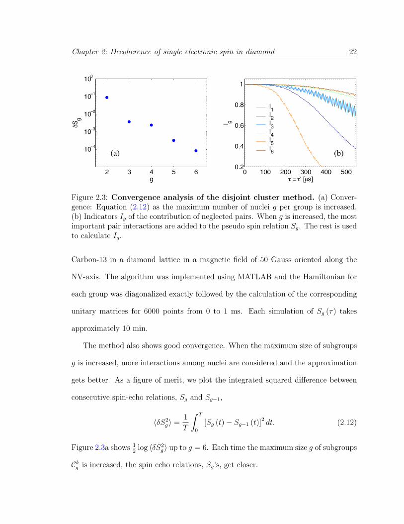
Figure 2.3: Convergence analysis of the disjoint cluster method. (a) Conver-gence: Equation (2.12) as the maximum number of nuclei g per group is increased.(b) Indicators Ig of the contribution of neglected pairs. When g is increased, the mostimportant pair interactions are added to the pseudo spin relation Sg. The rest is usedto calculate Ig.
Carbon-13 in a diamond lattice in a magnetic field of 50 Gauss oriented along the
NV-axis. The algorithm was implemented using MATLAB and the Hamiltonian for
each group was diagonalized exactly followed by the calculation of the corresponding
unitary matrices for 6000 points from 0 to 1 ms. Each simulation of Sg (τ) takes
approximately 10 min.
The method also shows good convergence. When the maximum size of subgroups
g is increased, more interactions among nuclei are considered and the approximation
gets better. As a figure of merit, we plot the integrated squared difference between
consecutive spin-echo relations, Sg and Sg−1,
〈δS2g 〉 =
1
T
∫ T
0
[Sg (t)− Sg−1 (t)]2 dt. (2.12)
Figure 2.3a shows 12
log 〈δS2g 〉 up to g = 6. Each time the maximum size g of subgroups
Ckg is increased, the spin echo relations, Sg’s, get closer.
Chapter 2: Decoherence of single electronic spin in diamond 23
In addition, following Ref. [58], we introduce the following indicator of all inter-
actions not included in groups Ckg , and therefore in Sg,
Ig (τ) =∏
n,mεCg
Snm (τ) . (2.13)
The product in Equation (2.13) runs over all neglected pair interactions contained
in Cg and Snm is calculated according to Equation (2.10). In this way, Ig (τ) has
the next order of smallest couplings for a given spin bath distribution and is an
indicator of convergence for our approach that obeys 0 ≤ Ig (τ) ≤ 1. When Ig (τ)
is close to unity, good convergence is achieved. Figure 2.3b shows Ig (τ) for several
aggregations (different g’s). As expected, when the maximum subgroup size g is
increased, the contribution from all neglected interactions is small. By the time the
neglected interactions become important, the pseudo-spin Sg (τ) has already decayed
(see Figure 2.2).
2.5 Results and Discussion
The results shown in Figure 2.4 clearly indicates that the electron spin echo signal
cannot be modeled by just one time scale. This result can be understood by noting
that few strongly interacting nuclei can coherently modulate the usual exponential
decay. This is in good quantitative agreement with recent experimental results[27].
The random distribution of the spin bath and the relative high coupling between
two nearest neighbor nuclei (∼ 2 kHz) may cause a few nuclei to contribute signif-
icantly to the decay of the spin-echo signal. Nuclei that makes small contributions
to the decoherence of the electron contribute as 1 − aτ 4 ≈ exp(−aτ 4) as it can be

Chapter 2: Decoherence of single electronic spin in diamond 24
seen from Equation (2.10). This behavior starts to deviate from exp(−aτ 4) as the
interaction between nuclei increases. Figure 2.4a shows a very unusual decay at which
few nuclei modulate coherently (Fig. 2.4b, black curve) the irreversible contribution
from the rest of the bath (Fig. 2.4b, red curve). Therefore, individual NV centers
can show a rich variety of spin-echo signals with multiple time scales. The coherent
modulation of the spin-echo diffusion due to strong interacting nuclei suggests that we
can think about a system composed of the electron and these few strong interacting
nuclei and an environment composed of the rest of the spin-bath.
Each NV center experiences a different random configuration and concentration
of Carbon-13. This causes a large distribution of decoherence times T2 when many
centers are probed. In order to estimate the decoherence time T2 we fit the envelope
of Sg (τ) to exp (−(2τ/T2)3). When the fit is not accurate we define T2 as the longest
time for which Sg ≥ 1/e. Figure 2.5a shows the histogram of T2 for 1000 different
random distribution of Carbon-13 in the diamond lattices for an external magnetic
field of 50 Gauss parallel to the NV-axis. Clearly, there exists substantial variation
in T2 for different centers.
As expected, the decoherence time decreases as the impurity concentration in-
creases. This is shown in Figure 2.5b where T2 goes as 1/n. To understand this it
is possible to make an analysis using a small τ expansion; while this is not always
correct, it provides a simple explanation of the underlying behavior. From Equation
(2.10), the decoherence time scales as the geometric mean of the bath dynamics and
the bath-spin interaction, i.e.,
T2 ∼(CAc
)−1/2, (2.14)

Chapter 2: Decoherence of single electronic spin in diamond 25
00 200200 400400 600600 800800 10001000 00
0.20.2
0.40.4
0.60.6
0.80.8
11
[ [ µµ
S S
s]s]
g=6
g=6 (( !!) )
!! = =! !""
(b)(a)
Figure 2.4: Example of spin echo signal modulated by a pair of Carbon-13. (a) Electron spin-echo signal highly modulated by a few Carbon-13 that stronglyinteract with the electron spin. (b) The strong contribution to the signal (black curve)has been isolated from the contribution from the rest of the spin bath (red curve).
where C is the averaged nuclear-nuclear dipolar interaction and Ac is some charac-
teristic value for the electron-nuclear interaction. Here we can make a connection
with phenomenological models and in particular with Equation (2.1). Free induction
decay rates are proportional to the interaction between the central spin and the bath,
T ∗2 ∼ A−1c . In turn, the correlation time of the nuclear bath is proportional to the
dipole-dipole interaction between nuclear spins, τc ∼ C−1. Combining the two times
and Equation (2.14) leads to Equation (2.1).
Since both interactions, A and C, decay as r−3 and the average distance between
bodies scales with the concentration as n−1/3, both interactions scale linearly in n.
Therefore, the decoherence time T2 decreases approximately as
T2 ∝ 1/n. (2.15)
For non-zero transverse magnetic fields, second order processes via the electron
spin (see Appendix A.4) make a substantial contribution to decoherence. Even in

Chapter 2: Decoherence of single electronic spin in diamond 26
200 400 600 800 101000 01200 14000
50
100
150
10
200
−1
T2 [µs]
100
Impurity Concentration [%]
T 2 [ms]
(a) (b)
Figure 2.5: Statistical behavior of spin echo signals for different lattice real-izations. Histogram of T2 for 1000 simulations at a magnetic field of 50 Gauss at anangle of θ = 0 (blue) and θ = 6 (red) with respect to the NV-axis. (b) Decoherencetime T2 versus impurity concentration, Carbon-13, at 50 Gauss along the NV axis.
the case of non-interactig nuclei, Equation (2.8), a transverse magnetic field causes
the revivals to diminish due to an enhanced nuclear g-factor experienced by nuclei
nearby the electron (see Equation (A.55) in Appendix A.4). To understand this effect,
consider that revivals occur because in each half of the spin-echo sequence each 13C
nuclear spin makes a full 2π Larmor precession (or multiples of it). Thus, in each half
of the spin-echo sequence the accumulated Zeeman shift, due to the AC component
of the 13C nuclear field, cancels regardless of the initial phase of the oscillating field
produced by the 13C nuclear spins. The 13C nuclear DC field component is refocused
by spin-echo. However, if different nuclei precess at different Larmor frequencies, Ω0n,
the accumulated Zeeman shifts for each nuclei cancels at different times and therefore
the total accumulated Zeeman shift will be non-zero, preventing a complete refocusing
of the electron spin. In addition, the average interaction between nuclei close to the
electron spin is enhanced due to the enhancement of their g factors (see Equation

Chapter 2: Decoherence of single electronic spin in diamond 27
0
00
45 90 135 1800
200
20
45
40
60
80
100
40090 600135 800
!
180
[deg]
B [G
auss
]
0
100
1000
200300
0
400
200
500600700800
0.2
400 0.4
600
800
0.6
0.8
! [deg]
T 2 [µs]
1
"="#
S(")
290 Gauss
(a)
(b) (c)
Figure 2.6: Magnetic field magnitude and alignment dependence. (a) Co-herent time T2 for different magnetic field strength and angles (measured from theNV-axis). Each point is average over 6 different random distributed baths. (b) Co-herence time T2 versus angle of the magnetic field for 4 different spin baths at 50Gauss. (c) Pseudo spin Sg=6 (τ) at 290 Gauss. At high fields the collapses due to theelectron-nuclear dynamics decreases (see text).
(A.55) in Appendix A.4). These effects are illustrated in Figure 2.5a for a magnetic
field at an angle of θ = 6 from the NV-axis and in Figure 2.6b.
As the angle between the magnetic field and the NV-axis, θ, is increased, the

Chapter 2: Decoherence of single electronic spin in diamond 28
electron-nuclear dynamics dominates and the spin-echo signal shows small revivals
and fits poorly to a single exponential decay. Thus, to describe the coherence time at
these angles, we have plot the average value of the signal, normalized by the average
signal at θ = 0:1
T2(B, θ) ≡ T2(B, θ = 0)
∫∞0|SB,θ(t)|dt∫∞
0|SB,θ=0(t)|dt . (2.16)
Figure 2.6a shows how the coherence of the signal varies with the strength and orien-
tation of the magnetic field. This map is averaged over 6 different spin baths, since
the random localization of Carbon-13 nuclei in the lattice makes the coherent time
to vary from NV-center to NV-center as it can be seen in Figure 2.6b for a fixed
magnetic field.
When the magnetic field along the NV-axis increases, the contribution from the
electron-nuclear interactions decreases (see Figure 2.6c). This happens because the
quantization axis for the nuclei points almost in the direction of the external magnetic
field producing a small oscillating field. This can be easily seen in the non-interacting
case, Equation (2.8), where the second term vanishes if Ω(0)n ‖ Ω
(1)n . Similarly, when
electron spin-echo is performed using the sub manifold ms = +1,−1, the signal
does not revive since each nuclei refocus the electron at different times. This occurs
because the Larmor frequencies in this case, Ω±1n , are position dependent and differ
for each nuclei.
We also point out that the approximation introduced in Section 2.2 is valid as long
as the impurity concentration of Carbon-13 is not too high, so the neglected interac-
1 We choose this approach as the signal has sufficiently non-trivial electron-nuclear dynamics forθ 6= 0 that fitting an envelope decay function, as is done for θ = 0, leads to large errors.

Chapter 2: Decoherence of single electronic spin in diamond 29
tions that connect different groups do not play an important role. This allows us to
treat the bath as isolated groups. A heuristic argument to evaluate the validity of the
present method is to consider the ratio between intra and inter group dipolar intera-
tions. We consider the root mean square (RMS) value of the dipolar interaction since
the interaction itself average to zero due to its angular dependance when an isotropic
distribution of nuclear spins is considered and due to the random initial spin config-
uration in the high temperature limit. The RMS contribution from a shell of spins
is proportional to I (rmin, rmax) =(∫ rmax
rminr−64πr2dr
)1/2
=((4π/3)(r−3
min − r−3max)
)1/2.
Therefore, the ratio between intra and inter group interactions can be estimated as
I (rnn, rg)/I (rg, R) ≈ (rg/rnn)1/2, where rnn is the nearest neighbor distance, rg is
the radius of the group that contains g nuclear spins and R is the radius of the spin
bath. For a given concentration of Carbon-13 nuclei n, the number of nuclear spins
g inside a sphere of radius rg is g = n × 8 × 4π(rg/a)3/3, where a is the size of the
unit cell which contains 8 Carbons. Under these considerations, the mentioned ratio
is√g/nNnn ≈
√g/4n, where Nnn is the number of Carbons inside a sphere of ra-
dius rnn for which we have assigned a conservative value of 4. For the concentration
of Carbon-13 (n ∼ 1%), this ratio is much larger than one, supporting the validity
of the current approximation. The approximation also relies on the relatively large
interaction between the central spin (electron) and the bath, An, when compared to
the intra-bath interaction, Cnm. The reason for this is that as the central spin gets
disconnected from the bath (reducing An), the decay occurs at later times τ and in-
teractions of the order of τ−1 start to play a role. To illustrate this, consider the size
of each subgroup scaling as (g/n)1/3 where g is the size of the subgroup. Then, the

Chapter 2: Decoherence of single electronic spin in diamond 30
interaction between nearest neighbor groups scales as nCnn/g where Cnn is the near-
est neighbor nuclear interaction. The time at which this interaction is important goes
as t ∼ g/nCnn = g/C. If we require this time to be larger than the decoherence time
(t T2), we find that the two types of interactions should satisfy g(Ac/C
)1/2 1
(for the present study this value is around 150). Therefore, when the interaction be-
tween the addressed spin and the bath is of the order of the intra-bath interactions,
the approximation breaks down. This would be the case of the spin-echo signal for
a nuclear spin proximal to the NV center[39] in which more sophisticated methods
should be applied such as tree tensor networks[62].
2.6 Comparison with experiments
Many of the results presented in previous sections have been confirmed exper-
imentally. In particular, Mizuochi et al.[66] confirmed the inverse proportionality
dependence with the concentration of Carbon-13 (Equation 2.15). In addition, the
measured and calculated values for the decoherence times agrees within 30%.
The dependence of T2 on the angle θ between the magnetic field and NV-axis,
described in Section 2.3.1 and Figure 2.6 has been confirmed by experiments per-
formed by Paul Stanwix, My Linh Pham, and David Lesage in Ronald Walsworth’s
laboratory[32]. In addition, they measured the power n of the decay function,
E(τ) ∝ exp− (τ/T2)n. (2.17)
As mentioned on Section 2.5, when the magnetic field is aligned with the NV axis,
the decay is due to dipole-dipole interaction among Carbon-13’s leading to a decay

Chapter 2: Decoherence of single electronic spin in diamond 31
with a power n varying between 3 and 4. Meanwhile, when the magnetic field is
misaligned, the value for the decay should be around n = 2. THe measurements of
Stanwix et al. agree with this analysis, finding higher values of n when the magnetic
field is aligned with the NV axis and lower values of n when the magnetic field is at
a non-zero angle. Interestingly, the values for n found at high angles are lower than
values predicted by theory for a single NV center. This difference is due to an average
effect present in ensemble measurements which is discussed as follow.
2.6.1 Ensemble measurements
In Section 2.3.1 we found that decoherence with an off axis magnetic field is
primarily caused by one or two Carbon-13’s nearby to the central NV spin. In an
ensemble measurement, the strength of this interaction has a large variation since it
is position dependent. For few NV centers in the ensemble, this interaction will be
big, but for most NV centers it will be small. Therefore, it is necessary to average
over the wide-ranging interactions experienced by all NVs in the ensemble to get the
form of the measured echo signal[67, 68],
E(t) =
∫f(b) exp(−bt2)db (2.18)
where f(b) is the probability distribution for having a value b of the NV-Carbon-
13 interaction. From Section 2.3.1 we can approximate this value by the hyperfine
interaction, Ak, between the nearest Carbon-13 nucleus and the central NV spin[67],
b = |Ak|2. (2.19)

Chapter 2: Decoherence of single electronic spin in diamond 32
In a cubic lattice with randomly distributed Carbon-13, this distribution is well ap-
proximated by (see Appendix A.3)
fb(b) = 2b−3/2
(1√bmin
− 1√bmax
). (2.20)
where
bmin =(µ0
4πγeγn
)2 1
r6max
bmax =(µ0
4πγeγn
)2 1
a6. (2.21)
Here, bmin is given by the size of the crystal (if very small) or the effective volume
(r3max) we assign for the average Carbon-13 nucleus; and bmax is determined by the
smallest distance between the nearest Carbn-13 nucleus and the central NV spin (set
by the diamond lattice spacing a). If this probability distribution is used, we obtain
the ensemble echo signals shown in Figure 2.7.
2.7 Conclusions
We have presented a method to evaluate the decoherence of a single spin in the
presence of an interacting randomly-distributed bath. It properly incorporates the
strong electron-nuclear dynamics present in NV centers and explains how it affects the
decoherence. We also incorporates the dynamic beyond the secular approximation by
including an enhanced nuclear g-factor that depend on the orientation of the external
magnetic field relative to the NV-axis and by including an electron mediated nuclei
interaction. Our results show that the spin echo signal for NV centers can present
multiple time scales where the exponential decay produced by many small nuclei
contributions can be coherently modulated by few strongly interacting nuclei. The

Chapter 2: Decoherence of single electronic spin in diamond 33
0 1 2 30
0.5
1
t (1/T2)
E(t)
0 1 2 30
0.05
0.1
b
f(b)
0 0.5 1 1.5 2 2.5 30
0.5
1
t (1/T2)
E(t)
with f(b) = b−3/2
exp(−t2)exp(−t)
b−3/2
GaussianLorentzian
! b−3/2 e−bt2 db
Figure 2.7: Averaging individual distributions of the NV-Carbon-13 in-teraction. a) Averaged signal (2.18) for several distributions f(b). Note that theaveraged signal obtained with f(b) = b−3/2 looks like gaussian decay at short timesbut exponential decay at long times. b) Distributions f(b) used to calculated theaveraged signal in (a). c) Again averaged signal E(t) using f(b) = b−3/2 for betterappreciation.
coherence times in ultra-pure diamond can be further improved by making isotopically
pure diamond with low concentration in Carbon-13. This method may be used in
other systems as long as the intra-bath interaction is smaller than the interaction
between the central spin and the bath. These results have important implications,
e.g., in magnetometry where long coherence times are important. For example, echo
signals persisting for up to milliseconds can be used for nanoscale sensing of weak
magnetic fields, as it was demonstrated recently[27].
Chapter 3
Magnetic field sensing with an
individual electronic spin in
diamond
3.1 Introduction
Sensitive solid-state magnetometers typically employ phenomena such as super-
conducting quantum interference in SQUIDs[34, 35] or the Hall effect in semiconductors[36].
Intriguing novel avenues such as magnetic resonance force microscopy (MRFM) are
also currently being explored[37, 38]. Our approach to magnetic sensing[25] uses the
coherent manipulation of a single quantum system, an electronic spin qubit. As illus-
trated in Figure 3.1, the electronic spin of an individual NV impurity in diamond can
be polarized via optical pumping and measured through state-selective fluorescence.
Conventional electron spin resonance (ESR) techniques are used to coherently ma-
34

Chapter 3: Magnetic field sensing with an individual electronic spin in diamond 35
nipulate its orientation. To achieve magnetic sensing we monitor the electronic spin
precession, which depends on external magnetic fields through the Zeeman effect.
This method is directly analogous to precision measurement techniques in atomic
and molecular systems[42], which are widely used to implement ultra-stable atomic
clocks[69, 70, 71] and sensitive magnetometers[72].
The principal challenge for achieving high sensitivity using solid-state spins is
their strong coupling to the local environment, which limits the free precession time
and thus the magnetometer’s sensitivity. Recently, there has been great progress in
understanding the local environment of NV spin qubits, including 13C nuclear spins
[51, 73, 53, 39, 74] and electronic spin impurities[75, 76, 77]. Here, we employ coherent
control over a coupled electron-nuclear system[25, 53], similar to techniques used in
magnetic resonance, to decouple the magnetometer spin from its environment. As
illustrated in Figure 3.2, a spin-echo sequence refocuses the unwanted evolution of the
magnetometer spin due to environmental fields fluctuating randomly on time scales
much longer than the length of the sequence. However, oscillating external magnetic
fields matching the echo period will affect the spin dynamics constructively, allowing
sensitive detection of its amplitude.
The ideal preparation, manipulation and detection of an electronic spin would
yield a so-called quantum-projection-noise-limited minimum detectable magnetic field[71]
δBmin ∼ ~gµB√T2T
(3.1)
where T2 is the electronic spin coherence time, T is the measurement time, µB is the
Bohr magneton, ~ is Planck’s constant, and g ≈ 2 is the electronic Lande g-factor. In
principle, for typical values of T2 ∼ 0.1-1 milliseconds, sensitivity on the order of a few

Chapter 3: Magnetic field sensing with an individual electronic spin in diamond 36
Figure 3.1: Principles of the individual NV electronic spin diamond mag-netic sensor. (a) A single NV impurity proximal to the surface of an ultra-purebulk single-crystal diamond sample (left) or localized within a diamond nano-crystal(right) is used to sense an externally-applied AC magnetic field (shown on the left).A 20 micron diameter wire generates microwave pulses to manipulate the electronicspin states (see Appendix B.3). (b) Level structure of the NV center. (c) Schematicof the experimental approach. Single NV centers are imaged and localized with ∼ 170nm resolution using confocal microscopy. The position of the focal point is movednear the sample surface using a galvanometer mounted mirror to change the beampath and a piezo-driven objective mount. A pair of Helmholtz coils are used to pro-vide both AC and DC magnetic fields. Experiments are then performed on single NVcenters as verified by photon correlations measurements.

Chapter 3: Magnetic field sensing with an individual electronic spin in diamond 37
nT/Hz1/2 can be achieved with a single NV center. Although this is less sensitive than
for state-of-the-art macroscopic magnetometers[33, 35], a key feature of our sensor
is that it can be localized within a region of about ten nanometers, either in direct
proximity to a diamond surface or within a nano-sized diamond crystal (Figure 3.1a).
Sensitive magnetic detection on a nanometer scale can then be performed with such a
system under ambient conditions. Figure 3.3 provides a comparison between magnetic
field sensitivity and detector volume for several state-of-the-art magnetometers and
the NV diamond systems demonstrated here.
Figure 3.2: Optical and microwave spin-echo pulse sequence used for sensingan AC magnetic field BAC(τ). An individual center is first polarized into themS = 0 sublevel. A coherent superposition between the states mS = 0 and mS = 1 iscreated by applying a microwave π/2 pulse tuned to this transition. The system freelyevolves for a period of time τ/2, followed by a π refocusing pulse. After a secondτ/2 evolution period, the electronic spin state is projected onto the mS = 0, 1 basisby a final π/2 pulse, at which point the ground state population is detected opticallyvia spin-dependent fluorescence. The DC magnetic field is adjusted to eliminate thecontribution of the randomly phased field produced by 13C nuclear spins (gold curve)by choosing τ = 2n/ωL, for interger n.

Chapter 3: Magnetic field sensing with an individual electronic spin in diamond 38
10−20
10−15
10−10
10−5
100
105
10−16
10−14
10−12
10−10
10−8
10−6
10−4
Se
nsitiv
ity (
T/H
z1/2
)
Detection volume (m 3)
SQUID 1 (1995)
BEC (2007)
Vapour Cell 1 (2007)
NV nanocrystal (2008)
SQUID 2 (2006)
Hall Probe 1 (2004)
Hall Probe 2 (2004)
Hall Probe 3 (2004)
Vapour Cell 2 (2003)
SQUID 3 (2003)
Hall Probe 4 (2002)
Hall Probe 5 (1996)NV single crystal (2008)
Figure 3.3: Sensitivity versus detection volume for various kinds of mag-netic sensors. At cryogenic temperatures, SQUID 1-3[78, 79, 80]; at room tem-perature, Hall Probe 1-3[81, 82], BEC[83], NV nanocrystal (this work) and NV inultra-pure diamond (projected from present bulk single-crystal studies); and at 100-200C, Vapour Cell 1-2[84],13.
3.2 Implementation of spin-based magnetometry
using NV centers
To establish the sensitivity limits of a single electronic spin magnetometer, we car-
ried out a series of proof-of-principle experiments involving single NV centers in bulk
ultra-pure single crystal diamond and in commercially available diamond nanocrys-
tals. Our experimental methodology is outlined schematically in Figure 3.1a; further
detail about our experimental setup and diamond samples are given in Appendices
B.1 and B.2. We first focus on the single crystal diamond bulk sample. Figure 3.4
shows a typical spin-echo signal observed from an individual NV center. The peri-
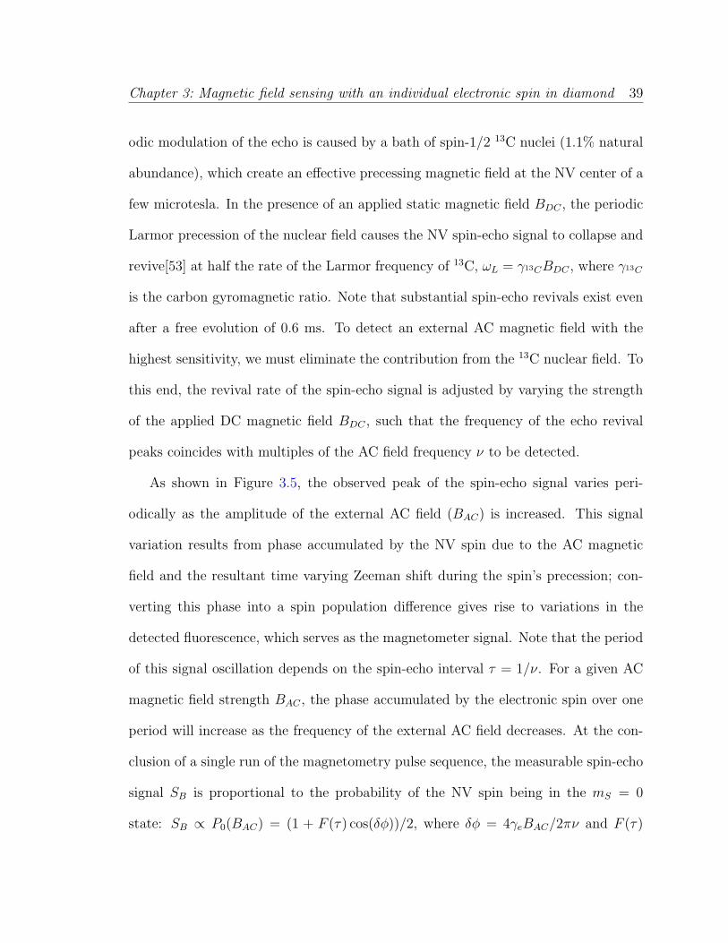
Chapter 3: Magnetic field sensing with an individual electronic spin in diamond 39
odic modulation of the echo is caused by a bath of spin-1/2 13C nuclei (1.1% natural
abundance), which create an effective precessing magnetic field at the NV center of a
few microtesla. In the presence of an applied static magnetic field BDC , the periodic
Larmor precession of the nuclear field causes the NV spin-echo signal to collapse and
revive[53] at half the rate of the Larmor frequency of 13C, ωL = γ13CBDC , where γ13C
is the carbon gyromagnetic ratio. Note that substantial spin-echo revivals exist even
after a free evolution of 0.6 ms. To detect an external AC magnetic field with the
highest sensitivity, we must eliminate the contribution from the 13C nuclear field. To
this end, the revival rate of the spin-echo signal is adjusted by varying the strength
of the applied DC magnetic field BDC , such that the frequency of the echo revival
peaks coincides with multiples of the AC field frequency ν to be detected.
As shown in Figure 3.5, the observed peak of the spin-echo signal varies peri-
odically as the amplitude of the external AC field (BAC) is increased. This signal
variation results from phase accumulated by the NV spin due to the AC magnetic
field and the resultant time varying Zeeman shift during the spin’s precession; con-
verting this phase into a spin population difference gives rise to variations in the
detected fluorescence, which serves as the magnetometer signal. Note that the period
of this signal oscillation depends on the spin-echo interval τ = 1/ν. For a given AC
magnetic field strength BAC , the phase accumulated by the electronic spin over one
period will increase as the frequency of the external AC field decreases. At the con-
clusion of a single run of the magnetometry pulse sequence, the measurable spin-echo
signal SB is proportional to the probability of the NV spin being in the mS = 0
state: SB ∝ P0(BAC) = (1 + F (τ) cos(δφ))/2, where δφ = 4γeBAC/2πν and F (τ)

Chapter 3: Magnetic field sensing with an individual electronic spin in diamond 40
0
0
50
0.1
100
0.2
150
0.3
200
0.4
250
0.5
30
0.6
20
20
10
15
0
10
5
0
BAC
(nT)
Sig
na
l (%
ch
an
ge
)
δ B
δS
2
1
2
1
Sig
na
l (%
ch
an
ge
)
a
b
τ (ms)
Figure 3.4: Example electronic spin-echo measurement. We plot the nor-malized echo signal corresponding to a fractional change of NV center fluorescence.Maximal signal corresponds to an average number of photons n = 0.03 detected dur-ing the 324 ns photon counting window of a single experimental run. Collapses andrevivals are due to interactions with a 13C nuclear spin bath. The revivals occur athalf the rate of the Larmor frequency of 13C (here set by BDC = 22 gauss). Thespin-echo signal envelope was fitted with an exponential decay function modulatedby a strongly interacting pair of nearby 13C (for more information see Appendix B.4).Magnetometer sensitivity experiments are performed at spin-echo revival peaks tomaximize signal.
is the amplitude of the spin-echo signal envelope in the absence of the external AC
magnetic field (Figure 3.4).
The sensitivity of the NV magnetometer to small variations in BAC , e.g., as de-
picted in the measurements shown in Figure 3.5, is given by δBmin = σNS /dSB, where
σNS is the standard deviation of the spin-echo measurement after N averages and
dSB is the slope of the spin-echo signal variation with BAC . Since maximum sen-
sitivity (i.e., smallest δBmin) occurs at maximum slope, all magnetometer sensitiv-
ity measurements were conducted at this point. This maximum slope is propor-

Chapter 3: Magnetic field sensing with an individual electronic spin in diamond 41
0
0
50
0.1
100
0.2
150
0.3
200
0.4
250
0.5
30
0.6
20
20
10
15
0
10
5
0
BAC
(nT)
Sig
nal (
% c
hange)
δ B
δS
2
1
2
1
Sig
nal (
% c
hange)
a
b
τ (ms)
Figure 3.5: Demonstration of spin-echo-based magnetometry with an indi-vidual NV electronic spin in a bulk diamond sample. Examples of measuredspin-echo signal as a function of applied AC magnetic field amplitude for two oper-ating frequencies ν1 = 3.15 kHz (red) and ν2 = 4.21 kHz (blue), corresponding torevivals 1 and 2 indicated in Fig. 2a. Each displayed point is a result of N = 7× 10⁵
averages of spin-echo sequences. The magnetometer is most sensitive to variationsin the AC magnetic field amplitude (δB) at the point of maximum slope, with thesensitivity being limited by the uncertainty in the spin-echo signal measurement (δS).We note that the cosine behavior of the signal with respect to AC magnetic field am-plitude can be changed to a sine by adjusting the phase of the third microwave pulseby 90 degrees. This change moves the point of maximum magnetometer sensitivityto near zero AC field amplitude.
tional to the spin-echo amplitude divided by the frequency of the oscillating field,
dSB ∝ F (1/ν)/ν. For a shot-noise limited signal with uncertainty σS in a single
measurement: σNS = σS/√N , where N = T/τ , T is the measurement time and τ is
the length of the spin-echo sequence. Hence the magnetometer sensitivity is expected
to scale as δBmin ∝√ν/F (1/ν).
Figure 3.6a shows example measurements of the sensitivity δBmin after one second
of averaging as a function of the AC magnetic field frequency ν = 1/τ . As this
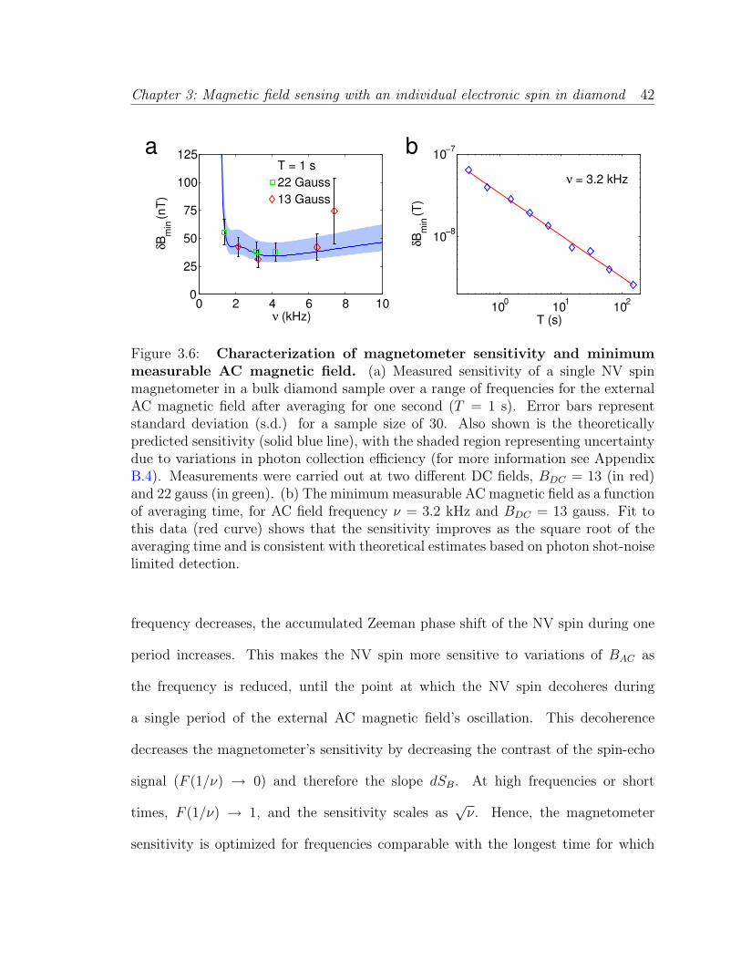
Chapter 3: Magnetic field sensing with an individual electronic spin in diamond 42
100
δB
min (
nT
)
10ν (kHz)
1
13 Gauss
22 Gauss
T = 1 s
0 2 1024 6 8 10
0
25
50 10−8
75
100
125 10−7
T (s)
δB
min (
T)
ν = 3.2 kHz
ba
Figure 3.6: Characterization of magnetometer sensitivity and minimummeasurable AC magnetic field. (a) Measured sensitivity of a single NV spinmagnetometer in a bulk diamond sample over a range of frequencies for the externalAC magnetic field after averaging for one second (T = 1 s). Error bars representstandard deviation (s.d.) for a sample size of 30. Also shown is the theoreticallypredicted sensitivity (solid blue line), with the shaded region representing uncertaintydue to variations in photon collection efficiency (for more information see AppendixB.4). Measurements were carried out at two different DC fields, BDC = 13 (in red)and 22 gauss (in green). (b) The minimum measurable AC magnetic field as a functionof averaging time, for AC field frequency ν = 3.2 kHz and BDC = 13 gauss. Fit tothis data (red curve) shows that the sensitivity improves as the square root of theaveraging time and is consistent with theoretical estimates based on photon shot-noiselimited detection.
frequency decreases, the accumulated Zeeman phase shift of the NV spin during one
period increases. This makes the NV spin more sensitive to variations of BAC as
the frequency is reduced, until the point at which the NV spin decoheres during
a single period of the external AC magnetic field’s oscillation. This decoherence
decreases the magnetometer’s sensitivity by decreasing the contrast of the spin-echo
signal (F (1/ν) → 0) and therefore the slope dSB. At high frequencies or short
times, F (1/ν) → 1, and the sensitivity scales as√ν. Hence, the magnetometer
sensitivity is optimized for frequencies comparable with the longest time for which

Chapter 3: Magnetic field sensing with an individual electronic spin in diamond 43
substantial echo signal is still observable. We note that it is possible to measure
at higher frequencies without further loss of sensitivity by using multiple spin-echo
pulses in a given measurement period [25]. Figure 3.6b shows examples of measured
NV magnetometer sensitivity for a fixed AC magnetic field frequency ν as a function
of measurement time T . The solid line is a fit to δBmin ∝ T−α, where α = 0.5± 0.01,
indicating that magnetic fields as small as few nanotesla are resolvable after 100
seconds of averaging.
As noted above, a key feature of our technique is that at specific times, determined
by echo revivals, the NV electronic spin can be decoupled from 13C nuclear spins to
leading order. In practice, the decoupling is not perfect due to the internal dynamics of
the electronic environment other than simple spin precession. In fact, the overall decay
of the echo signal shown in Figure 3.4 does not follow the simple exponential decay
associated with typical ESR on bulk samples. This can be understood by noting that
the echo dynamics of a single NV center near its revivals is likely determined by a few
nearby 13C, which interact strongly with the electronic spin[73, 51, 53, 39, 85], yielding
multiple characteristic time scales for echo decay (see Chapter 2 and Appendix B.4).
The absolute sensitivity of the NV magnetometer depends on the signal to noise
ratio in the readout of the NV electronic spin state. In the present demonstration, this
is limited by photon collection efficiency ≈ 0.1%. The resulting photon shot noise[33,
25] is about an order of magnitude larger than the ideal quantum projection noise limit
given by Equation (3.1), resulting in a corresponding degradation of magnetometer
sensitivity. Our theoretical prediction of magnetometer sensitivity (solid curve in
Figure 3.6a) combines the NV coherence properties shown in Figure 3.4 with the

Chapter 3: Magnetic field sensing with an individual electronic spin in diamond 44
00 55 10 10 151530
20
2025
1520
1510
105
5
BAC
(µT)
Sig
na
l (%
ch
an
ge
)
τ (µs)
Sig
na
l (%
ch
an
ge
) AC sensing
ba
Figure 3.7: Demonstration of magnetic sensing with a single NV electronicspin in a diamond nanocrystal. (a) Example electronic spin-echo signal froma single NV center contained in a diamond nanocrystal with diameter of 34 ± 12nm as determined by AFM. Maximum signal corresponds to an average number ofphotons n = 0.02 counted during a 324 ns photon counting window. The arrow lineindicates the time at which magnetic sensing is performed in Fig. 4b. (b) Exampleelectronic spin-echo signal as a function of the applied AC magnetic field amplitudeat a frequency of ν = 380 kHz. For this data, N = 2 × 10⁶ averages of spin-echo sequences were used. The resulting standard deviation yields a magnetometersensitivity of 0.5± 0.1 µT/Hz1/2.
noise due to photon counting statistics and imperfect collection efficiency (for more
information see Appendix B.4). This prediction is in excellent agreement with our
experimental results, indicating that our magnetometer is photon-shot-noise limited.
3.3 Magnetic sensing using diamond nanocrystals
To demonstrate magnetic sensing within a nanoscale detection volume, we also
performed similar experiments with single NV centers in diamond nanocrystals. We
used commercially available nanocrystals that contain a large number of impurities,
which shorten the electronic spin coherence time[86] to values ranging from 4 to 10

Chapter 3: Magnetic field sensing with an individual electronic spin in diamond 45
µs. Sensitive detection of AC magnetic fields is still possible as demonstrated exper-
imentally in Figure 3.7. Here, the echo signal from a single NV center in a 30 nm
size nanocrystal decays on the time scale of ∼ 4 µs. The absence of characteristic
collapses and revivals, associated with couplings to 13C nuclear spins, indicates that
the echo decay is likely due to other spin impurities such as paramagnetic substitu-
tional nitrogen atoms containing unpaired electron spins. Magnetic sensing with such
a nanocrystal at ν = 380 kHz is demonstrated in Figure 3.7b. From these measure-
ments we estimate a magnetometer sensitivity of δBmin ∼ 0.5± 0.1 µT/Hz1/2 for this
nanocrystal.
Improved magnetometer sensitivity for bulk and nanocrystal diamond may be
achieved in several ways. By using isotopically pure diamond with low concentra-
tions of both 13C and nitrogen electron spin impurities, much longer coherence and
interrogation times should be possible. For diamond nanocrystals, however, the ulti-
mate sensitivity will eventually be limited by surface effects [76, 87]. Increases to the
signal-to-noise ratio may also be possible by improving the measurement readout ef-
ficiency. Near single-shot readout of an electronic spin in diamond has been achieved
with cryogenic cooling using resonant excitation[23]. Photon collection efficiency
at room temperature can also be substantially improved using either conventional
far-field optics or evanescent, near-field coupling to optical waveguides[88]. Finally,
further improvements can likely be obtained by using magnetic sensing with multiple
NV centers and by employing more complex pulse sequences[25].

Chapter 3: Magnetic field sensing with an individual electronic spin in diamond 46
3.4 Outlook and Conclusions
Our results demonstrate that electronic spins in diamond can be used for preci-
sion measurements of nanoscale magnetic fields. This approach opens a new regime
of magnetic sensing, enabling detection of single electron and even nuclear spins sepa-
rated from NV centers by a few tens of nanometers, see SI. For example, by combining
our spin-echo based method with the recently demonstrated[28] transport and ma-
nipulation of nanocrystals using an atomic force microscope (AFM), a new kind of
nanoscale scanning magnetic sensor may be created. Such a sensor could have a
wide range of applications from biological and materials science to quantum informa-
tion processing and fundamental tests of quantum mechanics. With the aid of field
gradients, used for example in MRFM approaches[37, 38], NV diamond magnetome-
ters may allow sensing and resolving of individual nuclear spins with applications
in structural biology[25, 26]. It also provides an efficient method for measuring sin-
gle electronic spins in various quantum computing architectures. Furthermore, this
technique may allow non-destructive mapping of quantum states into NV centers,
operating as a quantum magnetic “head” [89], with possibilities for mechanical trans-
port of quantum information. Finally, we note that our technique could be used
for detecting the quantum motion of magnetic mechanical resonators[90, 91], with
new possibilities for creating nonclassical states of mechnical motion and for testing
quantum mechanics on a macroscopic scale.

Chapter 4
Repetitive readout of a single
electronic spin via quantum logic
with nuclear spin ancillae
4.1 Introduction
Efforts have recently been directed towards the manipulation of several qubits
in quantum systems, ranging from isolated atoms and ions to solid-state quantum
bits [92, 93]. These small-scale quantum systems have been successfully used for
proof-of-concept demonstrations of simple quantum algorithms [94, 95, 96, 97]. In
addition, they can be used for potentially important practical applications in areas
such as quantum metrology [92]. For example, techniques involving quantum logic
operations on several trapped ions have been applied to develop an improved ion state
readout scheme, resulting in a new class of atomic clocks [70, 98]. We demonstrate a
47

Chapter 4: Repetitive readout of a single electronic spin via quantum logic withnuclear spin ancillae 48
similar technique to enhance the readout of a single electronic spin in the solid state.
Our method makes use of quantum logic between a single electronic spin and
nuclear spin qubits in its local environment for repetitive readout. While such nuclear
spins are generally the source of unwanted decoherence in the solid-state, recent
theoretical [99, 85, 100] and experimental [73, 39, 45, 77, 101, 102, 103] work has
demonstrated that when properly controlled, the nuclear environment can become a
very useful resource, in particular, for long-term quantum memory.
Our experimental demonstration makes use of a single negatively-charged nitrogen-
vacancy (NV) center in diamond. The electronic ground state of this defect is an
electronic spin triplet (S = 1) and is a good candidate for a logic qubit, on account of
its remarkably long coherence times [104] and fast spin manipulation using microwave
fields [105]. Furthermore, the center can be optically spin polarized and measured
by combining confocal microscopy techniques with spin-selective rates of fluorescence
[73]. In practice, the NV spin readout under ambient, room temperature conditions
is far from perfect. This is because laser radiation at 532 nm for readout re-polarizes
the electronic spin before a sufficient number of photons can be scattered for the state
to be reliably determined.
4.2 Repetitive readout scheme
Our approach is to correlate the electronic spin logic qubit with nearby nuclear
spins [106], which are relatively unperturbed by the optical readout, prior to the mea-
surement process [74]. Specifically, we use one or more 13C (I = 1/2) nuclear spins
in the diamond lattice, coupled to the NV electronic spin via a hyperfine interaction,
Chapter 4: Repetitive readout of a single electronic spin via quantum logic withnuclear spin ancillae 49
as memory ancillae qubits. For example, a single 13C nuclear spin has eigenstates
|↑〉n1(aligned) or |↓〉n1
(anti-aligned) with the local magnetic field. The composite
electronic-nuclear system is first prepared in a fiducial state, |0〉e|↓〉n1, using a se-
quence of optical, microwave and radiofrequency (RF) pulses. Next, the electronic
spin is prepared in an arbitrary state |Ψ〉e = α|0〉e + β|1〉e, where |0, 1〉e denote elec-
tronic state with ms = 0, 1. Before readout, we perform a sequence of gate operations
resulting in the entangled electron-nuclear state |Ψ〉e |↓〉n1→ α |0〉e |↓〉n1
+β |1〉e |↑〉n1.
The optical measurement process projects this state into either |0〉e |↓〉n1or |1〉e |↑〉n1
.
When optically excited these two states fluoresce at different rates dependent on the
value of mS. Within a typical measurement period, less than one photon is counted
before the electron spin is repolarized to |0〉e, which indicates that the uncertainty of
the electronic spin state measurement is quite large.
The nuclear spin can thus reveal the former electronic state because of the cor-
relations established before the electronic spin was reset. To achieve this repetitive
readout, we perform a controlled-not operation, which maps |0〉e |↓〉n1→ |0〉e |↓〉n1
and
|0〉e |↑〉n1→ |1〉e |↑〉n1
, and repeat the optical measurement. Fluorescence counting of
these two states can be added to prior measurements to decrease the uncertainty for
electronic spin state discrimination. If optical readout does not destroy the orienta-
tion of the nuclear spin, the uncertainty in the determination of the electronic spin
can be reduced via repetitive measurements. In this way the overall signal-to-noise of
the measurement process of our logic qubit can be increased. After multiple readout
cycles and many quantum logic operations, the nuclear spin orientation will finally
be destroyed. However, it is possible to further improve the readout scheme by using

Chapter 4: Repetitive readout of a single electronic spin via quantum logic withnuclear spin ancillae 50
a pair of ancillary nuclear spins and imprinting the electronic state into a GHZ-like
state |Ψ〉e |↓〉n1|↓〉n2
→ α |0〉e |↓〉n1|↓〉n2
+ β |1〉e |↑〉n1|↑〉n2
. In such a case, the state
of the first nuclear spin after repetitive readout sequences can be periodically “re-
freshed” using the information stored within the second nuclear spin. These schemes
are closely related to a quantum non-demolition (QND) measurement [107, 108], as
the nuclear spin population operators In1,n2z do not evolve throughout the electronic
spin readout and constitute “good” QND observables. While imperfect optical NV
electronic spin detection precludes an ideal QND measurement, our scheme neverthe-
less allows substantial improvement in the spin readout.
4.3 Implementation with nearby 13C ancillae
To implement the repetitive readout technique we use a single NV center in di-
amond coupled to nearby 13C nuclear spins. These nuclear spins can be polarized,
fully controlled and provide a robust quantum memory even in the presence of op-
tical radiation necessary for electronic spin-state readout [39, 74]. This is achieved
through a combination of optical, microwave, and RF fields (Figure 4.1) and discussed
in Appendix C.1.
To control a single nuclear spin, we choose a NV center with a well-resolved
13C hyperfine coupling near 14 MHz. The degeneracy of the |ms = ±1〉e spin states
is lifted by applying a B0 = 30 gauss magnetic field along the NV axis. Under
these conditions, the transitions of the electronic spin (e) within the subspace of
|0〉e , |1〉e can be selectively addressed, conditioned on a certain nuclear state. The

Chapter 4: Repetitive readout of a single electronic spin via quantum logic withnuclear spin ancillae 51
MW1 !MW2 !
+!! ! " !=!
MW2 !
MW2 !
532 nm !
Readout ! Polarize e !
532 nm !
|!|2 !
|"|2 !
+!! ! " !RF !
Repeat !
Repeat !
A! B!
C
RF !
MW1 !
MW2 !
Detector !
532 nm ! detect !pump ! pump !
!"#$%&'())*+) !%",(! -($."/0!!"#$%&'())()
D E
Figure 4.1: Repetitive readout of an electronic spin. (A) Illustration of theNV center and its proximal 13C nuclear spins. Inset: Energy levels of the coupledspin system formed by the NV electronic spin (e) and the first proximal 13C nuclearspin (n1). With a static magnetic field applied along the NV axis, spin n1 keepsthe same quantization axis when spin e is |0〉e or |1〉e (see Appendix C.2). Whenspin n1 is |↓〉n1
(or |↑〉n1), the microwave field MW1 (or MW2) resonantly drives spin
e between |0〉e and |1〉e, which can implement the Cn1NOTe gate. When spin e is|1〉e, the radio-frequency RF field resonantly drives spin n1 between |↓〉n1
and |↑〉n1,
which can implement the Ce NOTn1 gate. (B) Illustration of repetitive readout. Thered down (up) arrow represents the electronic spin state |0〉e (|1〉e), and blue down(up) arrow represents the nuclear spin state |↓〉n1
(|↑〉n1). (C) Experimental pulse
sequences that polarize spin n1 to |↓〉n1and spin e to |0〉e, followed by various probe
operations, before fluorescence readout of spin e. (D) Measured electronic spin Rabioscillations driven by MW1 and MW2 fields, for polarized spin n1. The small wigglesfor MW2 are due to off-resonant driving of the majority population in the |↓〉n1
state.The data is in agreement for finite detunings and microwave power (solid curves).The right vertical axis shows the average counts for a single readout. The left verticalaxis shows the probability in the |0〉e state, obtained from the average counts (seeAppendix C.1). (E) Measured nuclear spin Rabi oscillation driven by the RF field.
model Hamiltonian for this system (Figure 4.1A) is,
H = (∆ + γeB0)Sz + γCB0In1z + ASz In1
z (4.1)
where ∆ = 2π × 2.87 GHz is the zero field splitting, A is the hyperfine interaction,

Chapter 4: Repetitive readout of a single electronic spin via quantum logic withnuclear spin ancillae 52
and γe and γC are the electronic and nuclear spin gyromagnetic ratios. Sz = 121 + Sz
is a pseudo-spin one-half operator for the electronic spin subspace, 1 is the identity
matrix, and In1z and Sz are the spin 1/2 angular momentum operators. Coherent
oscillations between the |0〉e and |1〉e states, conditioned on a single proximal nu-
clear spin (n1) in |↓〉n1(or |↑〉n1
), are selectively driven by the microwave field MW1
(or MW2). To control nuclear spin n1 a resonantly tuned RF field to address the
levels |1〉e |↓〉n1and |1〉e |↑〉n1
, which are energetically separated due to the hyperfine
interaction (Figure 4.1A), is used.
Following the initialization of spin e, spin n1 is polarized by applying MW1 and
RF π pulses, which transfers the polarization from spin e to spin n1. Rabi oscillations
of spin n1 are demonstrated (Figure 4.1E) by preparing spin e in the |1〉e state
irrespective of the state of spin n1 (using MW1 and MW2 π-pulses) and increasing
the RF pulse length.
This data indicates that we can achieve spin n1 preparation (polarization) and
readout with combined fidelity F ≡ 〈↓ |ρ′| ↓〉 ≥ 75%, where ρ′ is the reduced density
operator for spin n1.
We now turn to the demonstration of the repetitive readout technique. As illus-
trated in Figure 4.1D, the direct readout of electronic spin is imperfect. We define n0
and n1 as the total number of photons detected for the |0〉e and |1〉e states, respec-
tively, during a single measurement interval. The signal is defined as the difference
in average counts between the two spin states: A0 = n0 − n1 ≈ 0.005 (Figure 4.1D).
Experimentally, photon shot-noise dominates the fluctuations in the counts. Because
of this shot noise and the low average count (n0 ≈ 0.016), we need to average over

Chapter 4: Repetitive readout of a single electronic spin via quantum logic withnuclear spin ancillae 53
N ∼ 105 experimental runs to obtain the data in Figure 4.1D.
To improve the signal, we use two spins: e and n1. Both spins are first polarized to
the initial state |0〉e |↓〉n1. Next, we perform a unitary operation U(t), which prepares
the superposition state |Ψ1〉 = (α |0〉e + β |1〉e) |↓〉n1that we would like to measure.
Instead of immediately reading out the electronic spin, we use a controlled-not gate
(CeNOTn1 , achieved by an RF π pulse) to correlate spin e with spin n1(Figure 4.2A).
We then optically readout/pump spin e, leaving the spin system in the post-readout
state: ρpost = |0〉 〈0|e ⊗(|α|2 |↓〉 〈↓|+ |β|2 |↑〉 〈↑|)
n1. The state of spin n1 via the
electronic spin e by performing a controlled-not operation (Cn1NOTe, achieved by an
MW1 or MW2 π pulse) is then readout. This completes a one-step readout of spin
n1, which can be repeated.
As a direct illustration of the enhanced readout technique, Figure 4.2C shows the
accumulated signal for Rabi oscillations of the electronic spin obtained by adding M
subsequent repetitive readouts for each experimental run. This procedure results in
a ten-fold enhancement of spin signal amplitude.
In order to further quantify the performance of this technique, the noise added
with each additional repetitive readout must be considered. The repetitive readout
spin signal is defined as a weighted sum of difference counts Am associated with
mth readout: Sw(M) =∑M
m=1 wmAm. The average values of Am are determined
experimentally by measuring the difference in average counts associated with Rabi
oscillations for each m-th repeated readout. The wm allow us to weight the contribu-
tion of each repetitive readout to the overall signal. The noise corresponding to the
repetitive readout signal is ∆Sw(M) =√∑M
m=1w2mσ
2m. Here σm is the uncertainty of
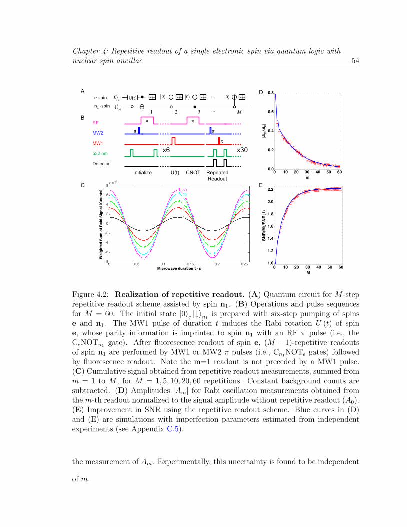
Chapter 4: Repetitive readout of a single electronic spin via quantum logic withnuclear spin ancillae 54
B!
C !
A! D !
E!
!"#$%& !
&'("#$%& !
)*+, !
0 10 20 30 40 50 60
1.0
1.2
1.4
1.6
1.8
2.0
2.2
M
SNR!M"#S
NR!1"
0 10 20 30 40 50 600.0
0.2
0.4
0.6
0.8
m
!A m"A0!RF !
MW1 !
MW2 !
Detector !
532 nm !x6
Initialize U(t) CNOT
x30
Repeated
Readout
Figure 4.2: Realization of repetitive readout. (A) Quantum circuit for M -steprepetitive readout scheme assisted by spin n1. (B) Operations and pulse sequencesfor M = 60. The initial state |0〉e |↓〉n1
is prepared with six-step pumping of spinse and n1. The MW1 pulse of duration t induces the Rabi rotation U (t) of spine, whose parity information is imprinted to spin n1 with an RF π pulse (i.e., theCeNOTn1 gate). After fluorescence readout of spin e, (M − 1)-repetitive readoutsof spin n1 are performed by MW1 or MW2 π pulses (i.e., Cn1NOTe gates) followedby fluorescence readout. Note the m=1 readout is not preceded by a MW1 pulse.(C) Cumulative signal obtained from repetitive readout measurements, summed fromm = 1 to M , for M = 1, 5, 10, 20, 60 repetitions. Constant background counts aresubtracted. (D) Amplitudes |Am| for Rabi oscillation measurements obtained fromthe m-th readout normalized to the signal amplitude without repetitive readout (A0).(E) Improvement in SNR using the repetitive readout scheme. Blue curves in (D)and (E) are simulations with imperfection parameters estimated from independentexperiments (see Appendix C.5).
the measurement of Am. Experimentally, this uncertainty is found to be independent
of m.

Chapter 4: Repetitive readout of a single electronic spin via quantum logic withnuclear spin ancillae 55
The signal-to-noise figure of merit is defined as SNR(M) = Sw(M)/∆Sw(M).
The wm weights are chosen by noting that the larger values of Am allow us to extract
more information given the fixed uncertainty of each measurement, and we should
emphasize these readouts more. As proven in Appendix C.4, the optimal choice of
weights corresponds to wm = |Am|/σ2m and the optimized SNR is given by:
SNRopt(M) =
√√√√ M∑m=1
∣∣∣∣Amσm∣∣∣∣2 (4.2)
In the ideal QND case, each repetitive readout would yield the same |Am| and the SNR
would scale with√M . For our experiment, the SNR saturates (Figure 4.2E) due to
the decay of the normalized amplitudes (Figure 4.3D). Nevertheless, the experimental
data shown in Figure 4.2E indicate the enhancement of SNR by more than 220%.
In assessing this result, it is noted that various imperfections can affect the repet-
itive readout, which leads to the imperfect first readout |A1| / |A0| < 1, the sharp
decrease in |A2|, and the subsequent exponential reduction |Am| = |A2|η(m−2) with
η ≈ 0.95.
These behaviors can be attributed to three major imperfections (see Appendix
C.5): errors from microwave pulses (about 7% error probability for each π pulse);
imperfect optical pumping of the electronic spin after each readout; and most sub-
stantially, the depolarization of the nuclear spin memory under optical illumination
To quantify the latter process, we study the decay times for 13C nuclear spins in
the presence of optical illumination. For an illumination time tL longer than 1 µs, the
nuclear spin polarization decays exponentially, with a characteristic time τn1 = 13 (1)
µs (Figure 4.3B). Since τn1 is much longer than the time for optical readout and
optical spin polarization of the NV electronic spin (350 ns), repetitive readout of e

Chapter 4: Repetitive readout of a single electronic spin via quantum logic withnuclear spin ancillae 56
A!
Exchange duration tX (µs) !
Pro
ba
bil
ity
in!
T!
C !MW1 !532nm !MW2 ! RF !MW1 ! RF ! 532nm !532nm !
532nm
Detect !Pulse
Sequence: !
B!
D !
!"#$%&'()*+) !"#$%&'()*,) -.&*)/012$*3() 4($5"67)*,)
Figure 4.3: Coherence and control of two nuclear spins. (A) The coupledspin system formed by the NV electronic spin (e) and two proximal 13C nuclear spins(n1 and n2). Middle inset: Energy levels for spins n1 and n2 when spin e is in the|0〉e state. Right inset: Schematic of flip-flop between spins n1 and n2, which iselectron-mediated by the second-order hopping via |1〉e |↓〉n1
|↓〉n2. (B) Measured de-
polarization of spins n1 and n2 under optical illumination. For the duration of opticalillumination tL longer than 1 µs, the polarizations for spins n1 and n2 decay exponen-tially with characteristic times τn1 = 13 (1) µs and τn2 = 53 (5) µs, respectively. FortL less than 1 µs, the decay is slightly faster, which is likely associated with dynamicsof the spin-fluctuator model that describe optically induced depolarization of singlenuclei (see ref. [74] and Appendix C.5). These decay times are much longer than theoptical readout/pump time of the electronic spin (about 350 ns). Inset: Log-linearplot. (C) Operations and pulse sequence to probe dynamics between spins n1 andn2. (D) Measured spin flip-flop dynamics between spins n1 and n2. For three differ-ent preparations of the initial state (|↓〉n1
|↑〉n2(cyan), |↓〉n1
and n2 in thermal state(black), and |↓〉n1
|↓〉n2(purple)), the observed population, pn1,↑ (t), oscillates with
the same period T = 117 (1) µs. These observations verify the theoretical prediction,with flip-flop coupling strength b = 4.27 (3) kHz.

Chapter 4: Repetitive readout of a single electronic spin via quantum logic withnuclear spin ancillae 57
is possible. (In the absence of optical illumination, the 13C nuclear spin decay times
are 1 ms [73, 39].) Despite the relatively long τn1 , after many cycles the nuclear
spin depolarizes. This degrades the repetitive optical readout for larger m, yielding
the overall exponential decay in the amplitude |Am| with increasing m (see Appendix
C.4).
As an indication of how this limit can be circumvented, the use of two ancillary
nuclear spins is considered. The state of spin e may be correlated with a more distant
spin n2, in addition to proximal spin n1. As the decay time of spin n2 is longer than
that of spin n1 due to a weaker interaction with spin e, the information stored in
spin n2 persists after spin n1 has been depolarized under optical illumination. This
remaining n2 polarization can then be transferred to spin n1 and repetitively readout
again.
Control of two nuclear spins is achieved by using the strongly coupled nuclear spin
n1 as a probe for the second nearby 13C nuclear spin n2, which cannot be directly
observed via the NV center. By placing the NV electronic spin in |0〉e state, the
hyperfine coupling is removed. This enables proximal 13C nuclear spins with similar
Zeeman energy to flip-flop and exchange spin population. Figure 4.3D shows that the
nuclear population, pn1,↑ (τ), oscillates between pn1,↑ (0) ≈ 0.2 and pn1,↑ (T/2) ≈ 0.5
with a period of T = 117 (1) µs (Figures 3A & 3C). The relatively high contrast
of these oscillations suggests an interaction with a second nuclear spin (n2), as the
two nuclei “flip-flop” between the states |↑〉n1|↓〉n2
and |↓〉n1|↑〉n2
. Such excitation
exchange requires a similar Zeeman splitting for the two spins, indicating that the
second nucleus is also a 13C. We note that the nuclear spin-spin interaction strength

Chapter 4: Repetitive readout of a single electronic spin via quantum logic withnuclear spin ancillae 58
determined by our measurements, b = π/T = 4.27 (3) kHz, is several times that of a
bare dipolar coupling (2 kHz for two 13C nuclei separated by the nearest neighbor dis-
tance, 1.54 A) signifying that their interaction is mediated by the NV electronic spin
(see inset of Figure 4.3A and Appendix C.2), which is described by the interaction
hamiltonian Hint = b(I1+I2− + I1−I2+). This interaction can be used to effectively
control the state of the second nucleus and of the entire three-spin system. Specif-
ically, a half period of nuclear spin oscillation, T/2, constitutes a SWAP operation
between the two nuclear spins. This operation can be used, e.g., to polarize the sec-
ond nuclear spin (Figures 3C, 3D). In addition, by modifying the initial state of spin
n1, we can prepare the initial state of the two nuclei in any of the four possible config-
urations: ↑↑, ↑↓, ↓↑, ↓↓ (see Appendix C.2). Further control is provided by putting
the electronic spin into the |1〉e state, in which case the flip-flop dynamics between
spins n1 and n2 disappears (see Figure C.3). This is because spins n1 and n2 typi-
cally have very distinct hyperfine splittings that introduce a large energy difference
(∆E b) between |↑〉n1|↓〉n2
and |↓〉n1|↑〉n2
and quench the interaction. Therefore,
we can implement a controlled-SWAP operation between spins n1 and n2, enabling
full control over spin n2. We further observe that spin n2 has decay time τn2 = 53 (1)
µs (Figure 4.3B inset) under optical illumination. Compared with spin n1, spin n2 is
less perturbed by the optical transitions between different electronic states, as it has
a weaker hyperfine coupling to the electron [74].
To demonstrate concatenated readout experimentally, both nuclear spins are ini-
tialized in the state |↓〉n1|↓〉n2
and a single NV electronic spin that we would like
to detect is prepared in a superposition state (α |0〉+ β |1〉)e. First, the operation

Chapter 4: Repetitive readout of a single electronic spin via quantum logic withnuclear spin ancillae 59
A!
B!
C !
!"#$%&' !
'("#$%&' !
')"#$%&' !
*#(!
+,-. !
*!
D !
x6 x6 x30 x30
0 20 40 60 80 100 120
1.0
1.1
1.2
1.3
1.4
1.5
1.6
M'
SNR!M'"#
SNR!1"
0 20 40 60 80 100 120
0.0
0.1
0.2
0.3
0.4
0.5
m
!A m"A0!
MW1 !
MW2 !
Detector !
532 nm!
Initialize
n1
U(t) Map Repeated
Readout
T/2!
SWAP Initialize
n1
T/2! T/2! T/2!
Repeated
Readout SWAP
RF !
Figure 4.4: Demonstration of two-level concatenated readout procedure.(A) Quantum circuit for concatenated M -step repetitive readout scheme assisted byboth spins n1 and n2. (B) Operations and pulse sequences for M = 60. Ideally, theGHZ-like state α |0〉e |↓〉n1
|↓〉n2+ β |1〉e |↑〉n1
|↑〉n2with the parity information of spin
e imprinted on both spins n1 and n2 is created before the first readout. After the firstround of M -step repetitive readout, spin n1 is depolarized, but spin n2 maintains itspolarization. The spin state of spin n2 is swapped to spin n1, which is then detectedduring the second round of M -step repetitive readouts. (C) Normalized amplitude|Am| / |A0| obtained from the m-th readout. (D) Measured improvement in the SNRusing the double repetitive readout scheme. The blue curves in (C) and (D) aresimulations with imperfection parameters estimated from independent experiments(see Appendix C.5).

Chapter 4: Repetitive readout of a single electronic spin via quantum logic withnuclear spin ancillae 60
(CeNOTn1-SWAP-CeNOTn1) is used to prepare the GHZ-type state |Ψ〉 = α |0〉e |↓〉n1|↓〉n2
+ β |1〉e |↑〉n1|↑〉n2
. Next, we optically readout/pump spin e, leaving the system in
state ρ′post = |α|2 |0 ↓↓〉 〈0 ↓↓|+ |β|2 |0 ↑↑〉 〈0 ↑↑|. M −1 repetitive readouts of spin n1
are then performed, in the manner described above, until spin n1 is depolarized. At
this point, spin n2 is still directly correlated with the first measurement of the e spin.
This information can be transferred to spin n1 by a nuclear SWAP gate. Thus, the
parity information can be measured again by performing a second round of M-step
repetitive readout. These operations are summarized in the quantum circuit (Figure
4.4A) and pulse sequences (Figure 4.4B).
Experimentally, the “revival” in the signal amplitude |Am| after the SWAP is
demonstrated (Figure 4.4C), which leads to an associated jump in the SNR curve
(Figure 4.4D) for M ′ = 61. This shows that the second nuclear spin can be used to
further enhance the readout efficiency. While ideally the repetitive readout scheme
assisted by two nuclear spins should improve the absolute SNR more than a single
nuclear spin, in the present experimental realization this is not yet so, as more errors
are accumulated for the two nuclear spin scheme due to initialization and pulse im-
perfections. These errors reduce the optical signal amplitudes for the readout assisted
by two nuclear spins, compromising the overall SNR improvement. Nevertheless, the
experiments clearly demonstrate that it is in principle possible to further boost the
relative SNR using additional nuclear spins.

Chapter 4: Repetitive readout of a single electronic spin via quantum logic withnuclear spin ancillae 61
4.4 Outlook and Conclusions
While we have demonstrated an enhancement for coherent Rabi oscillations, any
set of pulses acting on the electronic spin (e.g., a spin echo sequence) can be imple-
mented. This should have immediate applications to NV-based nano-magnetometry
[27, 28]. As the duration of the entire repetitive readout sequence (∼ 150µs in Figure
4.2B) is shorter than the typical echo duration in pure diamond, SNR improvements
directly translate into enhanced sensitivity and increased speed of nanoscale diamond
magnetometer [25]. This may have important applications in probing time-varying
processes in biophysical systems. The repetitive readout can also be used to achieve
single-shot readout of NV centers. At room temperature, with optimized collection
efficiency, an improvement in spin signal on the order of a few hundred is needed to
achieved single-shot readout. Potentially this improvement can be obtained by using
nuclei more robust to optical depolarization, such as the nitrogen nuclear spin of the
NV center in isotopically pure 12C diamond [104] and by using advanced control tech-
niques [109, 110] to suppress the imperfections from microwave pulses. Furthermore,
resonant optical excitations (λ ≈ 637 nm) can be used for NV centers at cryogenic
temperatures. Here the resolved spin structure of optical excited-states [111, 105, 112]
can be exploited to readout the electronic spin much more efficiently with reduced
perturbation to the nuclear spin [74]. Under these conditions, a ten-fold spin signal
improvement may be sufficient to enable single-shot readout of the NV electronic
spin. In turn, this can be employed to perform robust, adaptive QND measurements
of nuclear spin qubits which will be of direct use for distributed quantum networks
[106, 39]. Our experiments demonstrate that manipulation of several nuclear spin an-

Chapter 4: Repetitive readout of a single electronic spin via quantum logic withnuclear spin ancillae 62
cillae surrounding a central electronic spin can be used to implement useful quantum
algorithms in solid-state systems.
Chapter 5
Imaging and manipulation of
individual spins with nanoscale
resolution
5.1 Introduction
Optical techniques constitute powerful tools for spin detection and manipulation
that enable applications ranging from atomic clocks[40, 41] and magnetometers[42],
to quantum information processors[43, 39, 44, 45] and novel sensors and imaging
modalities for biological and life sciences[46, 25, 26, 27, 28, 104]. Several promis-
ing methods for fluorescence imaging have recently been developed to surpass the
diffraction limit and are already being applied to important problems in biology and
neuroscience[113, 114, 115] as well as sub-wavelength optical lithography[116, 117,
118]. For example, sub-diffraction imaging of fluorophores can be obtained by stimu-
63
Chapter 5: Imaging and manipulation of individual spins with nanoscale resolution64
lated emission depletion (STED) microscopy and related methods based on reversible
saturable optical linear fluorescence transitions (RESOLFT)[119, 47, 120, 121]. Using
optical fields with intensity zeros and steep spatial gradients, such as those provided
by doughnut-shaped beams, one can transiently switch the fluorophores to a different
state everywhere except for a small region near the vanishing optical intensity. In this
case the emitters from that small region can be separated from neighbours closer than
the diffraction limit. Since the emitters are switched to the designated (on or off)
state provided the optical stimulation rate exceeds that of the spontaneous decay rate
of that state, the ultimate resolution is, in principle, limited only by the applicable
optical power[121].
Our new approach to sub-diffraction spin detection and manipulation is outlined
in Figure 5.1. We consider an electronic spin system, such as the NV center in
diamond, which can be polarized via optical pumping, coherently manipulated with
resonant microwave radiation, and read-out with spin-state-dependent fluorescence.
Improved spatial resolution is achieved by illuminating the sample with a doughnut-
shaped optical beam just prior to optical spin readout. Spins positioned directly in
the center of the doughnut beam are not affected by it. However, spins that are
even a few nanometers away from the zero intensity position are re-polarized by the
doughnut beam and thus contribute differently to the fluorescence signal, providing
nanoscale imaging contrast. Moreover, selective coherent manipulation of a spin in
the doughnut center can be achieved by simultaneous exposure to resonant microwave
radiation and the optical doughnut beam (Figure 5.1c). The essence of this process is
that all coherent spin transitions away from the doughnut center are inhibited by the

Chapter 5: Imaging and manipulation of individual spins with nanoscale resolution65
Gaussian beam
Microwave ESR
Doughnut beam
Readout counter
tD
Spin manipulation
A B
b
a
532nm Laser& AOM switch
532nm Laser& AOM switch
APD single photon counter
MicrowaveESR source
Gaussianmode
Doughnutmode
Phase ramp Oil immersionobjective(NA = 1.3)
Dichroicmirror
x yPiezo scanner
Fluorescencecollection
650-800nmPBS
Diamond Sample
1A1
3E
2.87 GHz3A2
0
1
-1
!
k
"!
3A2
3E
c
Selective manipulation
Figure 5.1: Principles of sub-diffraction far-field optical imaging and magne-tometry of individual NV electronic spins in diamond (”spin-RESOLFT”).a, Experimental sequence using pulsed optical and microwave excitation. NV spinsare first optically pumped to ms = 0 using a Gaussian beam at 532 nm followedby microwave manipulation. Application of 532 nm doughnut beam re-polarizes theouter ring to ms = 0, allowing the spin-state of the central dark region to be indepen-dently read-out. b, Energy level diagram of NV center showing optical absorption (k)and fluorescence (γ) rates. NV electronic spins are optically pumped from |ms| = 1to ms = 0 spin states through non-radiative relaxation via the metastable 1A1 sin-glet state. Microwave fields at around 2.87 GHz coherently manipulate the NV spinstates. The differential spin-state population is measured via spin-state-dependentfluorescence in the red. c, Schematic of experimental approach. NV centers are im-aged using confocal microscopy by scanning the sample around the focal point usinga 3-axis piezo stage (see Appendix D.2 for more details on the setup). The doughnutbeam is generated by passing a Gaussian beam through a vortex waveplate (2π az-imuthally varying phase ramp). See Appendix D.3 for more information on how tocreate the doughnut beam.
Chapter 5: Imaging and manipulation of individual spins with nanoscale resolution66
laser field due to a quantum Zeno-like effect[48], thereby allowing coherent rotation
of an individual spin at the doughnut center.
5.2 Breaking the diffraction limit resolution
Before proceeding we note that STED and related RESOLFT techniques have
been demonstrated to be effective in systems containing metastable states[47], al-
though not spin states previously. A specific advantage of our present approach,
which we refer to as spin-RESOLFT, stems from the exceptionally long lifetimes as-
sociated with spin sublevels of electronic ground states, which can reach seconds and
exceed the lifetimes of electronic transitions by more than six orders of magnitude.
Optical transitions involving such ground-state spin levels can be differentially satu-
rated by scattering just a few photons. Therefore, spin-RESOLFT allows individual
electronic spins associated with NV centers to be imaged on the nanoscale, with sev-
eral orders of magnitude lower laser power than most other super-resolution imaging
techniques. This offers a significant advantages in many applications, especially to
biological systems. Alternatively, for a given power of the doughnut laser beam, spin-
RESOLFT allows a dramatic improvement in resolution relative to STED and other
RESOLFT approaches, potentially extending to sub-nanometer scales. We also note
that another method for resolving closely spaced spins employs large magnetic field
gradients[28], as in conventional magnetic resonance imaging. This method, however,
requires detailed knowledge of the magnetic gradient topography and is only possible
for spins that can be resolved spectrally in ESR or NMR measurements. In what fol-
lows we show that the present technique allows one to use far-field optical detection to
Chapter 5: Imaging and manipulation of individual spins with nanoscale resolution67
resolve individual spins spaced by sub-diffraction-limited distances, sense their local
magnetic environment, and perform coherent spin manipulation, even when ESR or
NMR measurements are not capable of resolving individual spins spectrally.
Our experimental demonstration makes use of individual NV centers on an ultra-
pure single crystal bulk diamond grown by chemical vapour deposition (CVD). The
centers were created by irradiating 109 cm−2 nitrogen ions with energy of 6 keV, cor-
responding to an estimated average implantation depth of 10 nm, as determined by
simulations. The sample was then annealed at 800 C, yielding an observed NV con-
centration of approximately 0.6 NV/µm2. To reliably distinguish shallow implanted
ions from natural NV centers, a rare isotope 15N was used (see Appendix D.1 for more
information on the implantation/annealing procedure). An electronic spin associated
with the NV triplet ground state can be optically polarized, coherently manipulated
using conventional electron spin resonance (ESR) techniques[93, 77], and read-out
through spin-state-dependent fluorescence[23] (see Figure 5.1b). NV centers in ultra
pure diamond display exceptional electron spin lifetimes (T1), approaching seconds
at room temperature[39, 104]. To realize sub-diffraction optical imaging and mag-
netometry using NV spins, we first polarize all NV centers in the field of view into
the ground spin state ms = 0 using a focused Gaussian beam; then drive ESR spin
transitions to the ms = +1 or −1 state, or to a coherent superposition of these
states; and subsequently use an optical doughnut beam to selectively re-polarize the
spins of nearby NV centers. NV centers located in regions of high intensity are op-
tically pumped to the |0〉 ground state, whereas an NV center located at the central
intensity zero remains unaffected and maintains its original state. Thus, spatial in-

Chapter 5: Imaging and manipulation of individual spins with nanoscale resolution68
formation associated with this central NV is encoded into its electronic spin state,
which is subsequently determined by diffraction limited optical readout of the NV flu-
orescence. Scanning the sample with respect to the beams and repeating the above
procedure allows sub-diffraction imaging of the NV centers in the field of view, as
well as sensitive nanoscale magnetometry at the location of each NV center due to
the Larmor precession of a coherent superposition of NV spin states (detectable via
spin-state-dependent fluorescence)[25, 27].
Figure 5.2 shows example sub-diffraction optical images of an NV electronic spin
in diamond, acquired using the spin-RESOLFT technique. A ten-fold improvement
of 1D resolution was obtained for a fixed power of approximately 2 mW, focused to a
diffraction limited spot of 0.07 µm2, by increasing the duration of the doughnut beam
pulse. A similar resolution improvement was achieved for much lower doughnut power
of about 0.1 mW, provided the decrease in power is compensated by an increase in
doughnut duration. These observations are in excellent agreement with predictions
from a simple model of the imaging resolution ∆r provided by our sub-diffraction
spin detection technique (see Appendix D.4):
∆r ≈ λ/2NA√1 + ΓtD
(5.1)
Here λ is the wavelength of the optical field, NA is the numerical aperture of the
objective, Γ characterizes the maximum rate of optical excitation out of spin state |1〉,
and tD is the duration of the doughnut beam. Note that the spin imaging resolution
is determined by the product of the power and duration of the doughnut beam: hence
sub-diffraction-limited resolution can be achieved with a laser power that is well below
optical saturation of the excited state (3E), provided that tD is sufficiently long. Since
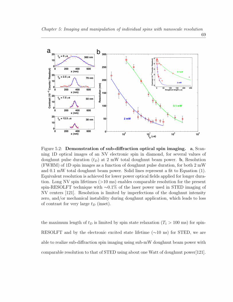
Chapter 5: Imaging and manipulation of individual spins with nanoscale resolution69
! "!! #!! $!!!
%!
"!&'()(!(µ*
+$!(,-
.(/,-0
! "!! #!! $!!!
%!
"!&'()("12(µ*
34(,-
.(/,-0
56,&78*&(/%!(!+(569,&*(:(;<8=69&0((((((((((((((((((((
! "!! #!! $!!!
%!
"!&'()(312(µ*
2!(,-
.(/,-0
! "!! #!! $!!!
%!
"!&'()(%"12(µ*
+>(,-
.(/,-0 %!!
%!%
%!"
%!+
!
2!
%!!
%2!
"!!
"2!
+!!
;<*6?9&@6,(/,-0
&'(/µ*0
"(-A
!1%(-A
a b
! "! #!! #"! $!! $"!
!
#
$
%
&
"
'()*+,-*./#!.!%.'(0)*-.1.23,4(0*5
6(078)0*.93)78*./µ-5
$.:;
!<#.:;
Figure 5.2: Demonstration of sub-diffraction optical spin imaging. a, Scan-ning 1D optical images of an NV electronic spin in diamond, for several values ofdoughnut pulse duration (tD) at 2 mW total doughnut beam power. b, Resolution(FWHM) of 1D spin images as a function of doughnut pulse duration, for both 2 mWand 0.1 mW total doughnut beam power. Solid lines represent a fit to Equation (1).Equivalent resolution is achieved for lower power optical fields applied for longer dura-tion. Long NV spin lifetimes (>10 ms) enables comparable resolution for the presentspin-RESOLFT technique with ∼0.1% of the laser power used in STED imaging ofNV centers [121]. Resolution is limited by imperfections of the doughnut intensityzero, and/or mechanical instability during doughnut application, which leads to lossof contrast for very large tD (inset).
the maximum length of tD is limited by spin state relaxation (T1 > 100 ms) for spin-
RESOLFT and by the electronic excited state lifetime (∼10 ns) for STED, we are
able to realize sub-diffraction spin imaging using sub-mW doughnut beam power with
comparable resolution to that of STED using about one Watt of doughnut power[121].
Chapter 5: Imaging and manipulation of individual spins with nanoscale resolution70
!"#!$%
&"#!$%
'()*(+,-
. ./0 ./1
.
./2
./0
./3
./1
!"#!$%
&"#!$%
456)!789:;<=
2
0
. ./0 ./1
.
./2
./0
./3
./1
0/> 0/? 0/@ 3
?A
@.
@A
2..
B6+C(D,EF"<CFGHF)+&"#IJK%
<-H(CF4+F)+F"#L"+M,)NF%
. A 2. 2A 0.
./0
./1
./O
./?
2
!"#!4%PC(Q,Q6-6R& 'F)RFC"2
. A 2. 2A 0.
./0
./1
./O
./?
2
!"#!4%
PC(Q,Q6-6R& 'F)RFC"0
. 0.. 1.. O.. ?.. 2...
.
./A
2
B6+C(D,EF"5H-4F"D6SRM"#)4%
PC(Q,Q6-6R& 'F)RFC"2
. 0.. 1.. O.. ?.. 2...
.
./A
2
B6+C(D,EF"5H-4F"D6SRM"#)4%
PC(Q,Q6-6R&
'F)RFC"0
a b
dc Gaussian
Microwave
Doughnut
Readout
Gaussian
Microwave
Doughnut
Readout
τ τ
Figure 5.3: Sub-diffraction optical magnetic sensing. a, Multiple NV centerscannot be identified or distinguished by their optically-detected ESR spectrum, ac-quired using confocal fluorescence microscopy. b, A conventional confocal image doesnot resolve multiple NV centers; whereas 2D spin imaging using spin-RESOLFT re-veals two NV centers separated by ∼150 nm. The conventional confocal image wastaken with an objective lens of numerical aperture of 1.3, leading to a spatial reso-lution of ∼250 nm. c, spin-RESOLFT provides spatially-selective measurements ofRabi oscillations for the two neighboring NV spins, which display stark differencesdue to different local magnetic field environments. d, spin-RESOLFT also enablesspatially-selective spin-echo measurements for the two NV spins, which reveal sub-stantial differences in spin coherence times, indicating the presence of magnetic im-purities in the local environment of NV Center 1. Solid lines in c and d are fits to amodel that includes the electronic spin of the NV center and the nuclear spin of thecenter’s 15N atom.

Chapter 5: Imaging and manipulation of individual spins with nanoscale resolution71
5.3 High resolution spin imaging and magnetom-
etry
To demonstrate simultaneous nanoscale spin imaging and magnetometry, we ap-
plied the spin-RESOLFT technique to NV centers in bulk diamond separated by less
than the diffraction limit. Figure 5.3a shows sub-diffraction 2D imaging of two NV
centers with identical ESR lines. In this case, it is not possible to identify the presence
of multiple centers using conventional confocal imaging and ESR techniques alone.
However, by using our new technique, the presence of two NV centers separated by
∼150 nm is directly revealed in a 2D sub-diffraction spin image (Figure 5.3b).
Detection of local magnetic fields with sub-diffraction resolution is presented in
Figures 5.3c,d. Specifically, when imaged individually with spin-RESOLFT, each NV
center exhibits a distinct modulation of its Rabi oscillation (Figure 5.3c), determined
by a relative shift in the center’s ESR transition frequency arising from small differ-
ences (< 1 G) in the static local magnetic field that each center experiences. Even
more subtle differences in the local magnetic field environment of the two NV centers
are revealed by sub-diffraction spin-echo measurements using spin-RESOLFT (Figure
5.3d). While at short times each of the centers display spin echoes modulated by Lar-
mor precession of the 15N nuclei in the applied static magnetic field, at longer times
the echo signals are substantially different. Center 2 displays good coherent dynamics,
evidenced by echo revivals exceeding 20 µs, whereas Center 1 shows no echo revival,
due to a nearby 13C nucleus[85] or other magnetic defects (see Appendix D.5). When
NV centers have different crystallographic axes and therefore different ESR spectra,
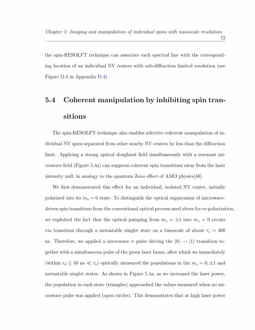
Chapter 5: Imaging and manipulation of individual spins with nanoscale resolution72
the spin-RESOLFT technique can associate each spectral line with the correspond-
ing location of an individual NV centers with sub-diffraction limited resolution (see
Figure D.3 in Appendix D.4).
5.4 Coherent manipulation by inhibiting spin tran-
sitions
The spin-RESOLFT technique also enables selective coherent manipulation of in-
dividual NV spins separated from other nearby NV centers by less than the diffraction
limit. Applying a strong optical doughnut field simultaneously with a resonant mi-
crowave field (Figure 5.4a) can suppress coherent spin transitions away from the laser
intensity null, in analogy to the quantum Zeno effect of AMO physics[48].
We first demonstrated this effect for an individual, isolated NV center, initially
polarized into its ms = 0 state. To distinguish the optical suppression of microwave-
driven spin transitions from the conventional optical process used above for re-polarization,
we exploited the fact that the optical pumping from ms = ±1 into ms = 0 occurs
via transition through a metastable singlet state on a timescale of about τs = 300
ns. Therefore, we applied a microwave π pulse driving the |0〉 → |1〉 transition to-
gether with a simultaneous pulse of the green laser beam; after which we immediately
(within τd ≤ 50 ns τs) optically measured the populations in the ms = 0,±1 and
metastable singlet states. As shown in Figure 5.4a, as we increased the laser power,
the population in each state (triangles) approached the values measured when no mi-
crowave pulse was applied (open circles). This demonstrates that at high laser power
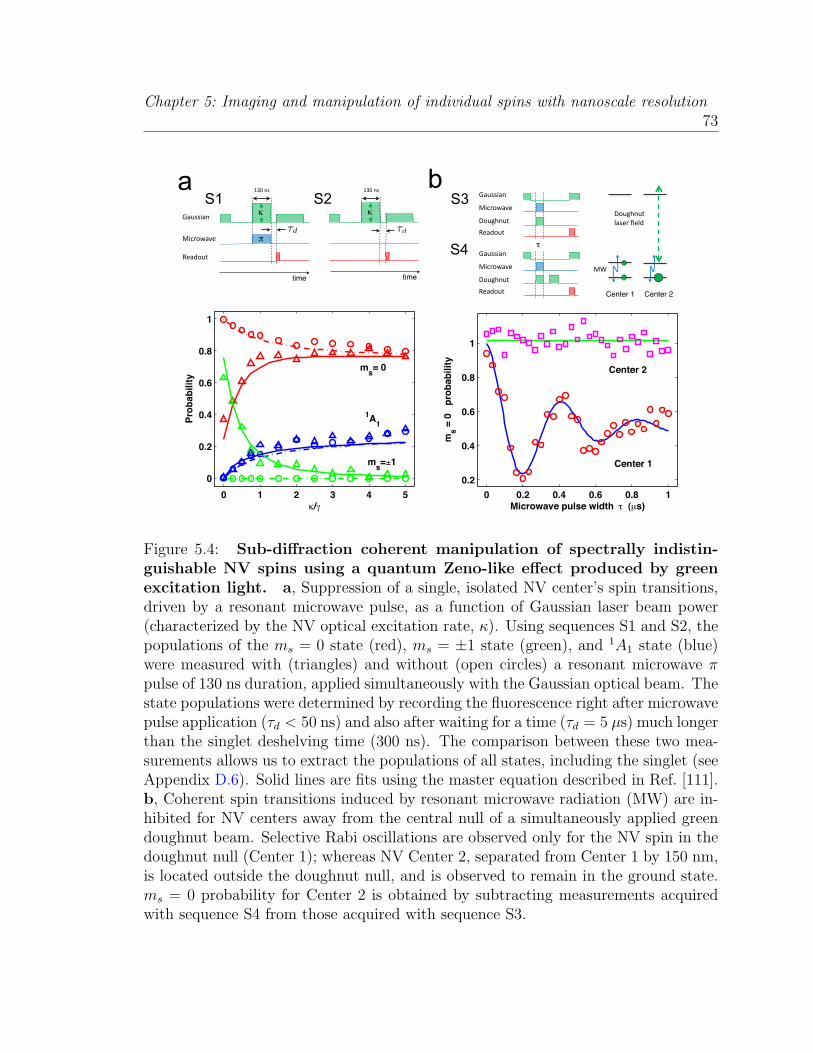
Chapter 5: Imaging and manipulation of individual spins with nanoscale resolution73
0 1 2 3 4 5
0
0.2
0.4
0.6
0.8
1
!/"
Pro
bab
ilit
y
0 0.2 0.4 0.6 0.8 1
0.2
0.4
0.6
0.8
1
Microwave pulse width # (!s)
ms =
0 p
rob
ab
ilit
y
ms= 0 Center 2
Center 1ms="1
1A
1
!"
#$%&'(%)*
+,-./*0.+1
a b
Center 1 Center 2
!23/$4,5.
6.,1$%)
7,%--2,(
89:*(-
S1 S2
time time
89:*(-
τd τd
S3
S4
#$%&'(%)
!23/$4,5.
6.,1$%)
7,%--2,(
#$%&'(%)
!23/$4,5.
6.,1$%)
7,%--2,(
Figure 5.4: Sub-diffraction coherent manipulation of spectrally indistin-guishable NV spins using a quantum Zeno-like effect produced by greenexcitation light. a, Suppression of a single, isolated NV center’s spin transitions,driven by a resonant microwave pulse, as a function of Gaussian laser beam power(characterized by the NV optical excitation rate, κ). Using sequences S1 and S2, thepopulations of the ms = 0 state (red), ms = ±1 state (green), and 1A1 state (blue)were measured with (triangles) and without (open circles) a resonant microwave πpulse of 130 ns duration, applied simultaneously with the Gaussian optical beam. Thestate populations were determined by recording the fluorescence right after microwavepulse application (τd < 50 ns) and also after waiting for a time (τd = 5 µs) much longerthan the singlet deshelving time (300 ns). The comparison between these two mea-surements allows us to extract the populations of all states, including the singlet (seeAppendix D.6). Solid lines are fits using the master equation described in Ref. [111].b, Coherent spin transitions induced by resonant microwave radiation (MW) are in-hibited for NV centers away from the central null of a simultaneously applied greendoughnut beam. Selective Rabi oscillations are observed only for the NV spin in thedoughnut null (Center 1); whereas NV Center 2, separated from Center 1 by 150 nm,is located outside the doughnut null, and is observed to remain in the ground state.ms = 0 probability for Center 2 is obtained by subtracting measurements acquiredwith sequence S4 from those acquired with sequence S3.

Chapter 5: Imaging and manipulation of individual spins with nanoscale resolution74
no population transfer occurs between the |0〉 and |1〉 states. Since our experiment
measured the populations before the metastable singlet could decay into the ground
state ms = 0, the data of Figure 5.4a directly confirms that the observed inhibition
of population transfer was not due to repumping out of the |ms| = 1 states. Instead,
the observed population dynamics indicates that the |0〉 to |1〉 population transfer
is suppressed by Zeno-like perturbations of the microwave spin transition induced
by light[48], along with partial (small) population transfer into electronic excited
states, in which microwave spin-changing transitions are also eliminated (For another
realization of the quantum Zeno effect involving NV centers see[122]).
We next employed spin-RESOLFT for selective coherent manipulation of one of
two closely spaced NV spins (Center 1 in Figure 5.3b), while the other NV spin
(Center 2) was kept in its ms = 0 state via the quantum Zeno-like effect. A pulsed
strong doughnut beam was applied simultaneously with a microwave pulse of variable
Rabi spin-flip angle, followed by optical measurement of the state of the NV spin
at the doughnut center. In a separate calibration experiment, the states of both
NV spins were measured together (no optical doughnut applied) as a function of
microwave pulse length (Rabi spin-flip angle). The spin-RESOLFT and calibration
measurements enabled us to determine the states of the two proximally spaced NV
spins individually. As shown in Figure 5.4b, spin transitions are inhibited for the NV
center outside the central null of the doughnut beam; whereas the central NV spin
undergoes coherent evolution, i.e., Rabi oscillations, in excellent agreement with a
theoretical model (blue and green curves in Figure 5.4b), as described in Appendix
D.6.
Chapter 5: Imaging and manipulation of individual spins with nanoscale resolution75
As shown in these demonstration experiments, the far-field optical resolution for
spin imaging and coherent manipulation is no longer limited by diffraction. We ex-
pect the resolution of the spin-RESOLFT technique to be even further improved by
technical upgrades such as increasing the contrast between the intensity of the dough-
nut crest and that of the central minimum, i.e., perfecting the doughnut zero[121].
In addition, implementing relatively large values of ΓtD, where Γ ∼ 100 MHz near
optical saturation and tD is on the order of the electronic spin lifetime T1 (which
ranges from 10 ms[39] to longer than a second in ultrapure diamond[104]), should
allow more than a 1000 fold improvement of resolution below the diffraction barrier,
making it feasible to attain sub-nanometer optical spin detection and manipulation,
including sensitive measurement of magnetic fields. Finally, the low levels of light re-
quired for our technique will also facilitate the parallelization of this imaging process
by replacing the scanning doughnut beam with moving arrays of lines or doughnuts of
vanishing intensity. This modification should enable fast camera-based spin imaging
over a large field of view.
5.5 Outlook and Conclusions
The capability to optically detect and manipulate individual spins with nanometer
resolution opens the door to a number of powerful applications in both the physical
and life sciences. For example, spin-RESOLFT could can be used for high fidelity
addressing of individual spin qubits in an array composed from NV centers separated
by distances in the range of 10-30 nm. In such a case, nearby electronic spins could be
coupled directly via magnetic or optical dipole-dipole interactions, thereby enabling

Chapter 5: Imaging and manipulation of individual spins with nanoscale resolution76
high fidelity two-qubit operations. By encoding qubits into nuclear spins nearby
to specific NV centers, and using spin-RESOLFT for sub-diffraction addressing of
electronic spins and control of electron-nuclear systems, both readout and coherent
manipulation could be enabled on nanometer scales, thereby opening a new route
to a room temperature scalable quantum information processor (see also[123]). More
specifically, the demonstrated Zeno-type inhibition of electronic Rabi oscillations (Fig-
ure 5.4b) allows for preparation, detection, and coherent manipulation of one nuclear
spin (associated with the NV center in the zero of the green doughnut-shaped beam)
without affecting qubits encoded in the nuclear spins of surrounding centers[74] (see
Appendix D.6). Likewise, intriguing applications in bioscience can be foreseen for
spin-RESOLFT, which combines high sensitivity magnetometry with sub-diffraction
imaging resolution. Examples include the use of NV-diamond nanocrystals in living
cells as photostable fluorescent biomarkers and sensors of nanoscale magnetic fields,
e.g., for direct imaging of activity in neuronal networks and mapping the local concen-
tration of reactive oxygen species and intra-cellular ions. In addition, by exploiting
long-lived ground electronic spin states, spin-RESOLFT has the potential for reaching
extraordinary imaging and sensing resolution with modest laser power levels, which
may be of interest for a diversity of super-resolution imaging applications involving,
in particular, biological systems. Finally, we expect that our approach can be ap-
plicable to a wide variety of spin systems, from trapped atoms and ions to quantum
dots, which may enable a diverse range of interesting applications in quantum science
and engineering.
Chapter 6
Group theoretical description of
the nitrogen-vacancy center in
diamond
6.1 Introduction
During the last five years nitrogen-vacancy (NV) centers have become potential
candidates for a number of applications at ambient conditions ranging from mag-
netometry [25, 26, 27, 28] to high spatial resolution imaging[121] and to quantum
computation[23]. At low temperature, the optical transitions of the NV center become
very narrow and can be coherently manipulated. This can be used to explore inter-
esting applications such as spin-photon entanglement generation[124] and all optical
control[125]. For these applications to be efficiently implemented, it is crucial to have
a detailed understanding of the excited state properties of this defect. Several studies
77

Chapter 6: Group theoretical description of the nitrogen-vacancy center in diamond78
have addressed this issue both experimentally[111, 112] and theoretically[126, 127].
Furthermore, other atom-like defects can potentially be engineered in diamond[20]
and other materials with similar or perhaps better properties suitable for the de-
sired application. Therefore, it is of immediate importance to develop a formalism to
analyze and predict the main properties of defects in solids.
Here we present such a formalism based on a group theoretical description. While
we focus on applications to the nitrogen-vacancy center in diamond, our formalism
can be applied to any point defect in solid state physics. Our method takes advantage
of the symmetry of the states to properly treat the relevant interactions and their
symmetries. We apply group theory to find out not only the symmetry of the eigen-
states but also their explicit form in terms of orbital and spin degrees of freedom. We
show that this is essential to build an accurate model of the NV center. In particular,
we analyze the effect of the Coulomb interaction and predict that the ordering of
the triplet and singlet states in the ground state configuration is 3A2,1E, 1A1 and
that the distance between them is on the order of the exchange term of the electron-
electron Coulomb energy. This ordering has been debated over the last few years and
our results agree with recent numerical calculations[128]. Our method is also used
to analyze important properties of the center such as selection rules. The explicit
form of the states helps us to realize a particularly useful lambda-type transition for
spin-photon entanglement generation. We show that from the excited state A2(3E)
the electron can decay to the ground state 3A2 ms = 1 (ms = −1) by emitting a right
(left) circularly polarized photon. We demonstrate that this is a consequence of the
spin-orbit interaction. This process is particularly robust due to the spin-spin inter-

Chapter 6: Group theoretical description of the nitrogen-vacancy center in diamond79
action in the excited state. We also consider perturbations that lower the symmetry
of a point defect, such as strain and electric field. In particular we show how the
polarization properties are affected in the presence of strain. We also show that the
non-axial spin-orbit interaction proposed in Ref. [129] should not mix the eigenstates
of the center in a given multiplet as the spin-orbit interaction remain invariant under
the symmetries of the C3v point group. In particular, it should not mix the states of
the lower branch of the excited state. Instead, we find that the spin-spin interaction is
responsible for the spin state mixing of the excited as a result of the lack of inversion
symmetry of the center. We analyze possible sources of mixing between the states.
Finally, we analyze the effect of electric fields via the inverse piezoelectric effect and
contrast with experimental findings. We show that this can be used to tune the po-
larization properties of optical transitions and the wavelength of emitted photons,
which is of direct importance for photon-based communication between NV centers.
Our study clarifies important properties of NV centers and provides the foundation
for entanglement between electronic spins and photons in solid state physics.
Our manuscript is organized as follow. In Section 6.2 we present a general group
theoretical formalism to calculate the electronic or hole representation of a point
defect for a given crystal field symmetry and number of electrons contained in the
defect. Next, we use group theory and the explicit form of the states to analyze the
effect of the Coulomb interaction between electrons (Section 6.3) and spin-spin and
spin-orbit interactions for the NV center (Sections 6.5 and 6.4, respectively). Next,
we analyze the selection rules of the unperturbed defect in Section 6.6. Finally, in
Section 6.7 we analyze the effect of strain and electric field perturbations.

Chapter 6: Group theoretical description of the nitrogen-vacancy center in diamond80
6.2 State representation
We are particularly interested in quasi-static properties of defects in crystals where
the complex electronic structure can be seen spectroscopically. In this limit one can
apply the Born-Oppenheimer approximation to separate the many-body systems of
electrons and nuclei. It relies on the fact that nuclei are much slower than electrons.
In this approximation the nuclei are represented by their coordinates and the physical
quantities of the electrons depend on these coordinates as (external) fixed parameters.
A defect in a crystal breaks down the translational symmetry reducing the symmetry
of the crystal to rotations and reflections. These symmetries form a point group which
in general is a subgroup of the point group of the lattice. The loss of translational
symmetry indicates that the Bloch-states are no longer the solution of the point
defect. In fact, some states can be very well localized near the point defect. These
defect states are particularly important in semiconductors and insulators when they
appear within the fundamental band gap of the crystal.
In the tight binding picture, the electron system of the diamond crystal may be
described as the sum of covalent-type interactions between the valence electrons of
two nearest neighbor atoms. When defects involve vacancies, the absence of an ion
will break bonds in the crystal, producing unpaired electrons or dangling bonds, σi,
which to leading order can be used to represent the single electron orbitals around the
defect. The particular combination of dangling bonds that form the single electron
orbitals ϕr is set by the crystal field of the defect and can be readily calculated
by projecting the dangling bonds on each irreducible representation (IR) of the point

Chapter 6: Group theoretical description of the nitrogen-vacancy center in diamond81
group of the defect[130],
ϕr = P (r)σi =lrh
∑e
χ(r)e Reσi, (6.1)
where χ(r)(e) is the character of operation, e (element), for the IR, r, lr is the dimen-
sion of the IR r and h is the order of the group (number of elements). A detailed
application of Equation (6.1) for the case of the NV center can be found in Appendix
E.1. There are two non-degenerate totally symmetric orbitals a1(1) ad a2(1) that
transform according to the IR A1, and there are two degenerate states ex, ey that
transform according to the IR E. At this stage, group theory does not predict the
energy order of these states. However a simple model of the electron-ion Coulomb
interaction can help to qualitatively get the order of the levels[131]. In Appendix E.1
we model the effect of this interaction on the single electron orbitals, ϕr, for the case
of the NV center and find that the ordering of the states (increasing in energy) is
a1(1), a1(2) and ex, ey. Indeed, ab initio density functional theory (DFT) calcula-
tions revealed [63, 18] that the a1(1) and a1(2) levels fall deeper than the ex and ey
levels which demonstrates the strength of group theory for qualitative predictions.
Once the symmetry and degeneracy of the orbitals is determined, the dynamics
of the defect is set by the number of electrons available to occupy the orbitals. The
orbitals with higher energy will predominantly set the dynamics of the defect. The
spin character of the defect will be determined by the degeneracy of the orbitals and
the number of electrons in them leading to net spins S = 0, 1, 2, ... if this number
is even and S =
12, 3
2, ...
if odd.
In the case of the negatively charged NV center, each carbon atom contributes one
electron, the nitrogen (as a donor in diamond) contributes two electrons and an extra
Chapter 6: Group theoretical description of the nitrogen-vacancy center in diamond82
electron comes from the environment [18], possibly given by substitutional nitrogens
[132]. The ground state configuration consists of four electrons occupying the totally
symmetric states and the remaining two electrons pair up in the ex, ey orbitals. In
this single particle picture, the excited state configuration can be approximated as
one electron being promoted from the a1(2) orbital to the ex,y orbitals[63].
If two more electrons were added to any of these configurations, the wavefunction
of the defect would be a singlet with a totally symmetric spatial wavefunction, equiv-
alent to the state of an atom with a filled shell [133, 134]. Therefore, the electronic
configuration of this defect can be modeled by two holes occupying the orbitals ex,y in
the ground state (e2 electronic configuration) and two holes in the orbital a1(2) and
ex,y for the excited state (ae electronic configuration). A third electronic configura-
tion, a2 can be envisioned by promoting the remaining electron from the orbital a1(2)
to the orbitals ex,y. Hole and electron representations are totally equivalent and it is
convenient to choose the representation containing the smallest number of particles.
If a hole representation is chosen, some care must be taken, as some interactions
reverse their sign, such as the spin-orbit interaction [133]. In what follows, we choose
a hole representation containing two particles (instead of an electron representation
containing four particles), since it is more convenient to describe the physics of the
NV center. However, the analysis can be applied to electrons as well.
The representation of the total n-electron wavefunction, including space and spin
degrees of freedom, is given by the direct product of the representation of each hole
and its spin ΓΨ =∏
n
(Γhn ⊗D 1
2
), where D 1
2is the representation for a spin 1
2
particle in the corresponding point group. The reduction or block diagonalization of
Chapter 6: Group theoretical description of the nitrogen-vacancy center in diamond83
the representation ΓΨ gives the eigenstates of the hamiltonian associated with the
crystal field potential and any interaction that remains invariant under the elements
of the point group in question. These interactions include spin-orbit, spin-spin and
Coulomb interactions, as well as expansions, contractions, and stress where their
axes coincide with the symmetry axis of the defect. The eigenstates can be found
by projecting any combination of the two electron wavefunction onto the irreducible
representations of the group [130, 135],
Ψr = P (r)ϕ1ϕ2 =lrh
∑e
χ(r)∗e Reϕ1Reϕ2, (6.2)
where ϕi can be any of the orbitals in Equation (6.1) and the subindex i refers
to the hole i. In the case of the NV center, it is illustrative to note that the spin
representation for the two particles can be reduced to D1/2⊗D1/2 = A1+A2+E, where
A1 corresponds to the singlet state, and A2 and E to the triplet state with zero and
non-zero spin projections, respectively. A list of the eigenstates and their symmetries
for the two hole representation can be found in Table 6.1 for the ground state (e2)
and the excited state (ae). For completeness, we include the doubly excited state (a2)
electronic configuration although this state is not optically accessible in the excitation
process of the NV center in experiments. Note that each electronic configuration
might have singlet and triplet states. The calculation performed to obtain Table 6.1
is similar to the calculation made to find the eigenstates when two spin particles
are considered. However, in this case one should use the Wigner coefficients of the
corresponding irreducible representation of the point group under consideration.
Group theory can predict why the hyperfine interaction with the nuclear spin of
the nitrogen in the excited state is more than an order of magnitude larger than in

Chapter 6: Group theoretical description of the nitrogen-vacancy center in diamond84
the ground state for both nitrogen species: the non-zero spin density in the ground
state wavefunction of the NV center is mostly concentrated in the orbitals ex,y which
have no overlap with the nitrogen atom. On the other hand, in the excited state,
when one electron is promoted from the a1(2) orbital to one of the ex,y orbitals,
the non-zero spin density comes now from unpaired electrons occupying the orbitals
a1(2) and ex,y. As the orbital a1(2) occupies the nitrogen atom, a sizable contact
term interaction between the electronic spin and the nuclear spin of the nitrogen is
expected [18, 105, 136].
Up to now, eigenstates inside a given electronic configuration have the same en-
ergy, however the inclusion of the electron-electron Coulomb interaction will lift the
degeneracy between triplets and singlets. This lifting can be of the order of a fraction
of an eV and it is analyzed for the ground state configuration of the NV center in Sec-
tion 6.3. Furthermore, the degeneracy inside triplet states is lifted by spin-orbit and
spin-spin interactions of the order of GHz, where the crystal field plays an important
role. These interactions will be treated in sections 6.4 and 6.5.
6.3 Ordering of singlet states
For a given eletronic configuration, the most relevant interaction is the electron-
electron Coulomb interaction, which is minimized when electrons are configured in
an antisymmetric spatial configuration. As the total wavefunction must be antisym-
metric for fermionic particles, the spin configuration must be symmetric. As a result,
the state with the largest multiplicity lies lower in energy. This analysis, known as
the first Hund’s rule, estimates that the ground state of the NV center should be

Chapter 6: Group theoretical description of the nitrogen-vacancy center in diamond85
Table 6.1: Partner functions of each irreducible representation for the direct prod-uct of two holes. The first column show the electronic configuration and betweenparenthesis their triplet (T) or singlet (S) character. The last column shows thename of the states given and their symmetry. In the table α(β) reads spin ↑(↓)and E± = |ae± − e±a〉, where e± = ∓(ex ± iey), |X〉 = (|E−〉 − |E+〉)/2 and|Y 〉 = (|E−〉+ |E+〉)i/2.
Conf. State Name
e2 (T) |exey − eyex〉 ⊗
|ββ〉|αβ + βα〉|αα〉
3A2−(E1)3A20 (A1)3A2+(E2)
e2 (S)|exex − eyey〉|exey + eyex〉|exex + eyey〉
⊗ |αβ − βα〉1E1 (E1)1E2 (E2)1A1 (A1)
ea (T)
|E−〉 ⊗ |αα〉 − |E+〉 ⊗ |ββ〉 A1 (A1)|E−〉 ⊗ |αα〉+ |E+〉 ⊗ |ββ〉 A2 (A2)|E−〉 ⊗ |ββ〉 − |E+〉 ⊗ |αα〉 E1 (E1)|E−〉 ⊗ |ββ〉+ |E+〉 ⊗ |αα〉 E2 (E2)
|Y 〉 ⊗ |αβ + βα〉 Ey (E1)|X〉 ⊗ |αβ + βα〉 Ex (E2)
ea (S)|a1x+ xa1〉 ⊗ |αβ − βα〉 1Ex (E1)|a1y + ya1〉 ⊗ |αβ − βα〉 1Ey (E2)
a2 (S) |a1a1〉 ⊗ |αβ − βα〉 1A1 (A1)
the triplet 3A2 state. We now address the question related to the order of singlets in
the ground state electronic configuration e2. The order of singlet states has a great
significance in understanding the spin-flipping fluoresence of the NV center, and ab
initio DFT calculations were unable to address this issue properly due to the many-
body singlet states. Since we have the explicit form of the wavefunctions we can work
out the ordering of the singlets in a given electronic configuration by analyzing the
expectation value of the Coulomb interaction, which can be written in the general
form,
Cabcd =
∫dV1dV2a
?(r1)b? (r2)V (|r1 − r2|) c (r1) d (r2) .

Chapter 6: Group theoretical description of the nitrogen-vacancy center in diamond86
Using this expression we find that in the ground state electronic configuration (e2),
the Coulomb interactions for these states are
C(3A2) = (Cxyxy − Cxyyx − Cyxxy + Cyxyx) /2
C(1E1) = (Cxyxy + Cxyyx + Cyxxy + Cyxyx) /2
C(1E2) = (Cxxxx − Cxxyy − Cyyxx + Cyyyy) /2
C(1A1) = (Cxxxx + Cxxyy + Cyyxx + Cyyyy) /2, (6.3)
where x, y correspond to ex, ey states. From this set of equations we find that the
spacing between the singlets 1A1 and 1E2 is equal to the spacing between the singlet
1E1 and the ground state 3A2, i.e., C(1A1)− C(1E2) = C(1E1)− C(3A2) = Cxxyy +
Cyyxx ≡ 2e, where the difference is the exchange energy. In addition, as 1E1 and
1E2 belong to the same irreducible representation E, it can be shown that C(1E2) =
C(1E1) (see Appendix E.2). Under this consideration, the ordering of the singlets is
3A2,1E, 1A1 with relative energies 0, 2e, 4e. It should be noted that, in this case,
the most symmetric state has higher energy since the Coulomb interaction between
two electrons is repulsive. This picture might be modified by the following effect. As
the Coulomb interaction transforms as the totally symmetric IR, the matrix elements
between states with the same symmetry are non-zero. The states 1E(e2) and 1E(ae)
can couple via the Coulomb interaction, increasing the gap between them. A similar
effect happens with the states 1A1(e2) and 1A1(a2). We note that, even taking into
account these corrections, our basic results here serve as a qualitative estimate for
the energy of the levels. Furthermore, in Equation (E.1) we did not take into account
the effect of the other electrons present in the system. Nevertheless, our approach
provides useful insight into the structure of the NV center. A very recent many-body
Chapter 6: Group theoretical description of the nitrogen-vacancy center in diamond87
perturbation theory (MBPT) calculation calculated the energy of singlet states [128]
and supported our conclusion.
6.4 Spin-Orbit interaction
In the previous section the electronic spin did not directly enter into the equa-
tions. For instance, the energy of the MS = 0,±1 sublevels of the 3A2 ground state
would have exactly the same energy. However, if the electronic spin is taken into
account, one can infer from Table 6.1 that in general the MS = 0 and MS = ±1
projections transform as functions of different IRs. For example, in the ground state
3A2, the MS = 0 projection transforms as the IR A1, while the MS = ±1 projections
transforms as the IR E. This implies that the projections do not share the same
eigenenergies of the system. Since these states are orbitally degenerate, the spin-
spin and spin-orbit interactions may account for the splitting of orbitally degenerate
states.
The spin-orbit interaction lifts the degeneracy of multiplets that have non-zero
angular momentum and it is also responsible for transitions between terms with dif-
ferent spin states[133]. It is a relativistic effect due to the relative motion between
electrons and nuclei. In the reference frame of the electron, the nuclear potential, φ,
produces a magnetic field equal to ∇φ× v/c2. In SI units, this interaction is given by
HSO =~
2c2m2e
(∇V × p) ·( s
~
), (6.4)
where V = eφ is the nuclear potential energy, me is the electron mass and p is
the momentum. The presence of the crystal field breaks the rotational symmetry

Chapter 6: Group theoretical description of the nitrogen-vacancy center in diamond88
of this interaction. Since φ is produced by the nuclear potential, it transforms as
the totally symmetric representation A1, and therefore ∇V = (Vx, Vy, Vz) trans-
forms as a vector. For a given point group, it is possible to identify the IRs to
which these components belong. In the case of C3v symmetry, their components
transform as (E1, E2, A1). As p also transforms as a vector, the term ∇V × p =
(Vypz − pyVz, pxVz − Vxpz, Vxpy − pxVy)∝ (Lx, Ly, Lz) transforms as the IRs (E2, E1, A2) =
(E,A2). This implies that the expectation values for the orbital angular operators
break into two classes: 〈lx〉 = 〈ly〉 and 〈lz〉. Therefore, the spin-orbit interaction has
the following form:
HSO = λxy (lxsx + lysy) + λzlzsz. (6.5)
The non-zero matrix elements of the angular momentum operators li in the basis
a, ex, ey can be determined by checking if (ϕi, lk, ϕf ) ⊃ A1 and are shown in Table
6.2 where A = 〈ey|lx|a〉, B = 〈ex|lz|ey〉 and C = 〈ex|lx|a〉. For a perfect Td or spherical
symmetry, A = B and C = 0. It is also useful to think about e± as p± orbitals and
a1(2) as pz orbitals, where the angular momentum operators satisfy l±a1(2) ∝ e±[137].
Table 6.2: Matrix elements for orbital operators in the C3v point group. For spheri-cally symmetric potentials, A = B and C = 0.
lx ex ey aex 0 0 −iCey 0 0 iAa iC −iA 0
ly ex ey aex 0 0 −iAey 0 0 −iCa iA iC 0
lz ex ey aex 0 iB 0ey −iB 0 0a 0 0 0
Once it is known how spin-orbit acts on the orbitals, ex, ey and a, it is possible to
calculate the effect of this interaction on the 15 states given in Table 6.1. An important
effect is the splitting in the excited state triplet between the states A1, A2 and Ex, Ey
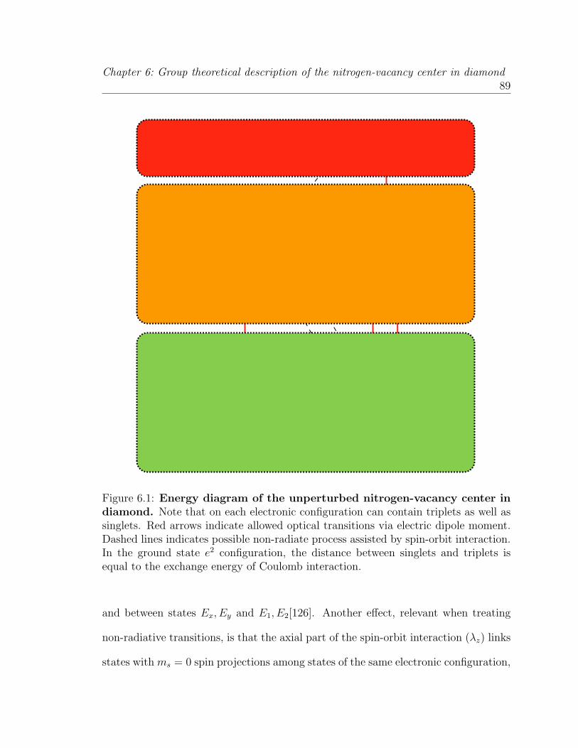
Chapter 6: Group theoretical description of the nitrogen-vacancy center in diamond89
1 E 1,2
1A1
E1,2
(A2)
(Ex, Ey)
A1
A2
A1
1A1
λ⊥(S+L− + S−L+)/2
λzSzLz
λzSzLz
λ⊥(S+L− + S−L+)/2
Ex
Ey
E1E2
ααββ
1Ex1Ey
E1,2
1E1,2
1A1
Ex,y
E1,2
(A2)
(Ex, Ey)
A1
A2
A1
1A1
1Ex,y
λ⊥(S+L− + S−L+)/2
λzSzLz
λzSzLz
λ⊥(S+L− + S−L+)/2
e
e
e2
ae
a2
Figure 6.1: Energy diagram of the unperturbed nitrogen-vacancy center indiamond. Note that on each electronic configuration can contain triplets as well assinglets. Red arrows indicate allowed optical transitions via electric dipole moment.Dashed lines indicates possible non-radiate process assisted by spin-orbit interaction.In the ground state e2 configuration, the distance between singlets and triplets isequal to the exchange energy of Coulomb interaction.
and between states Ex, Ey and E1, E2[126]. Another effect, relevant when treating
non-radiative transitions, is that the axial part of the spin-orbit interaction (λz) links
states with ms = 0 spin projections among states of the same electronic configuration,
Chapter 6: Group theoretical description of the nitrogen-vacancy center in diamond90
while the non-axial part (λ⊥) links states with non-zero spin projections with singlets
among different electronic configurations. In Figure 6.1 we show the states linked
by the axial and the non-axial parts of the spin-orbit interaction, for which non-
radiative transitions might occur. In addition to the well known transition between
A1(ae) → 1A1(e2), we find that this interaction might also link E1,2(ae) → 1E1,2(e2)
and in particular Ex,y → 1Ex,y(ae). The latter transition may play an important role,
as recent ab initio calculations have shown that the singlets 1Ex,y might lie very close
in energy to the excited state triplet [128]. In our model, the non-axial part of the
spin-orbit interaction, λ⊥ (l+s− + l−s+), does not mix the states of the excited state
triplet with different spin projections because the raising and lower operators, l− and
l+, link states of different electronic configurations.
We have numerically evaluated the ratio between the axial part and transverse
part of spin-orbit, λz/λxy = B/A = 0.75 using the functions ex and ey and a1(2)
from ab initio calculations (see Appendix E.5). This suggest that if the axial part
of spin-orbit is 5.5 GHz [112], the non-transverse part should be on the order of 7.3
GHz. We also have numerically confirmed that the non-axial part of spin orbit does
not mix the states on the excited state triplet, as the matrix elements of the raising
and lowering angular momentum operator applied over the states ex, ey is zero, i.e.
〈ei|lx,y|ej〉 = 0.
6.5 Spin-spin interaction
The spin-spin interaction between electrons is usually not present in systems with
spherical symmetry, due to the traceless character of the magnetic dipole-dipole in-

Chapter 6: Group theoretical description of the nitrogen-vacancy center in diamond91
teraction. However, if the electron wavefunction is not spherically distributed, this
interaction does not average out. Here we would like to describe its effect on the
excited state triplet of the NV center as well as to provide numerical estimation for
its strength. The spin-spin interaction can be written (in SI units) as,
hss = −µ0
4π
g2β2
r3(3(s1 · r)(s2 · r)− s1 · s2) , (6.6)
where si = 12
[σx, σy, σz] is the spin operator of particle i and σ are the Pauli matrices,
β is the Bohr magneton, g is the Lande-factor for the electron and µ0 is the magnetic
permeability of free space1. In order to analyze the effect of this interaction in the
defect it is useful to write the spatial and spin parts separately in terms of the irre-
ducible representations of the point group. Then, it is straightforward to express this
interaction in terms of the eigenstates of the defect (see Appendix E.3),
Hss = ∆ (|A1〉〈A1|+ |A2〉〈A2|+ |E1〉〈E1|+ |E2〉〈E2|)
−2∆ (|Ex〉〈Ex|+ |Ey〉〈Ey|)
+2∆′ (|A2〉〈A2| − |A1〉〈A1|)
∆′′ (|E1〉〈Ey|+ |Ey〉〈E1| − i|E2〉〈Ex|+ i|Ex〉〈E2|) . (6.7)
Figure 6.2 shows the effect of spin-orbit and spin-spin interactions on the excited
state manifold. In particular, we find that the state A2 has higher energy than the
state A1 contrary to previous estimations[126],2. In addition, we find that the spin-
spin interaction mixes states with different spin-projections. This effect is the result
1The contact term does not contribute due to the Pauli exclusion principle.
2Recently, this was indirectly experimentally confirmed. The lower energy state A1 was observedto have a shorter lifetime than the state A2[124]. This is as expected since the state A1 decaysnon-radiatevely to the singlet 1A1 via non-axial spin-orbit.

Chapter 6: Group theoretical description of the nitrogen-vacancy center in diamond92
A1, A2, E1, E2
Ex, Ey
A1
A2
E1, E2∆
2∆Ex, Ey
4∆′
λz
λz
Spin-orbit Spin-spinSpin-spin
(mixing part)
αE1 − βEy,
αE2 − βEx
αEy + βE1,
αEx + βE2,
Figure 6.2: Splitting due to spin-orbit and spin-spin interaction in tripletae. In addition to the splitting between different spin projections, spin-spin splitsstates A1,2. Our theory predicts the A2 state over the A1 state. As state A1 hasan additional non-radiative decay channel, it is possible to confirm this finding bymeasuring the lifetime of the state. Note that the splitting between A1 and A2 is adirect consequence of spin-orbit mixing the spatial and spin part of the wavefunction.
of the lack of inversion symmetry of the NV center and it is not present in systems
with inversion symmetry such as free atoms or substitutional atoms in cubic lattices.
This has no contradiction with group theory as the mixed states transform according
to the same IR (e.g. the E1 and Ey states transform both according to the IR E1,
see Table 6.1). The gaps between the ms = ±1 and ms = 0 projections and between
A1 and A2 states are given by
3∆ = 3µ0
4πg2β2
⟨X
∣∣∣∣1− 3z2
4r3
∣∣∣∣X⟩ = −3
4Dzz (6.8)
4∆′ = 4µ0
4πg2β2
⟨X
∣∣∣∣3x2 − 3y2
4r3
∣∣∣∣X⟩ = Dx2−y2 , (6.9)

Chapter 6: Group theoretical description of the nitrogen-vacancy center in diamond93
while the mixing term is given by
∆′′ =µ0
4πg2β2
⟨X
∣∣∣∣ 3xz
2√
2r3
∣∣∣∣X⟩ . (6.10)
We have evaluated numerically the values for this interaction using the orbitals ex
and ey from ab initio calculations (see Appendix E.5). To avoid numerical divergences
when r = 0, we estimate Equations (6.8) and (6.9) in reciprocal space following
reference [138]. We find that the zero field splitting on the ground state is 2.2 GHz
compared to the 2.87 GHz found experimentally. Meanwhile, for the excited state, we
find that 3∆ = 0.2 GHz and 4∆′ = 2.5 GHz. This is compared with the experimental
values 1.4 GHz and 3.3 GHz measured in [112].
We emphasize that, contrary to the ground state of the NV center, the splitting
between A1 and A2 in the excited state exists because the spin-orbit interaction
mixes the spin and spatial parts. In fact, at high temperatures, where the spin-orbit
interaction averages out [127], and if the spatial part is given by |X〉〈X| + |Y 〉〈Y |,
it can be checked by looking at Equation (E.5) that only the zero field splitting
∆es survives from the electronic spin-spin interaction, as confirmed by experiments
[105, 127].
6.6 Selection rules and spin-photon entanglement
schemes
Group theory tells us which transitions are dipole allowed by checking if the matrix
element contains the totally symmetric IR, 〈ϕf |e|ϕi〉 ⊃ A1. In the case of the NV
center (C3v), the only non-zero matrix elements are 〈a|x · r|ex〉 and 〈a|y · r|ey〉, from
Chapter 6: Group theoretical description of the nitrogen-vacancy center in diamond94
which it is straighforward to calculate the selection rules among the 15 eigenstates
given in Table 6.1 for the unperturbed center. This is shown in Table 6.3. These
matrix elements have been confirmed by our first principles calculations of these
matrix elements in the velocity representation as well as by other authors only for
the triplet transition [139]. Interestingly, since the excited state triplet has non-zero
angular momentum, photons emitted to the ground state must have left or right
circular polarization in order to preserve total angular momentum. In addition to the
well known triplet-triplet transition [140], transitions are allowed between singlets
of different electronic configurations. We remark that the transition between singlet
1A1(e2) and singlet 1E(e2) is not strictly forbidden by group theory in the first order,
but since both states belong to the same electronic configuration, no dipole moment
exists between them and the probability of radiative transition is extremely low. The
ratio between the dipole transition matrix elements associated with the triplet states
and those of the singlet states is about 5×10⁻⁹, according to our calculations with
the use of wave functions from first principles calculations. This transition might
be allowed by phonons or mixing of the states with singlets of different electronic
configurations. Regarding recent experiments by Rogers et al., where they identified
an emission from singlet to singlet[127], we think it is related to the 1E(ae) →1
A1(e2) transition. The transition 1A1(e2)→1 E(e2) might be possible for the reasons
described above, but it is unlikely to be sizable. A recent MBPT calculation supports
our conclusion [128]. A suitable experiment to unravel this issue will be to look at
the presence of this emission under resonant excitation. In this case, if the state
1E(ae) is above the excited state triplet, the state 1E(ae) will be hardly populated
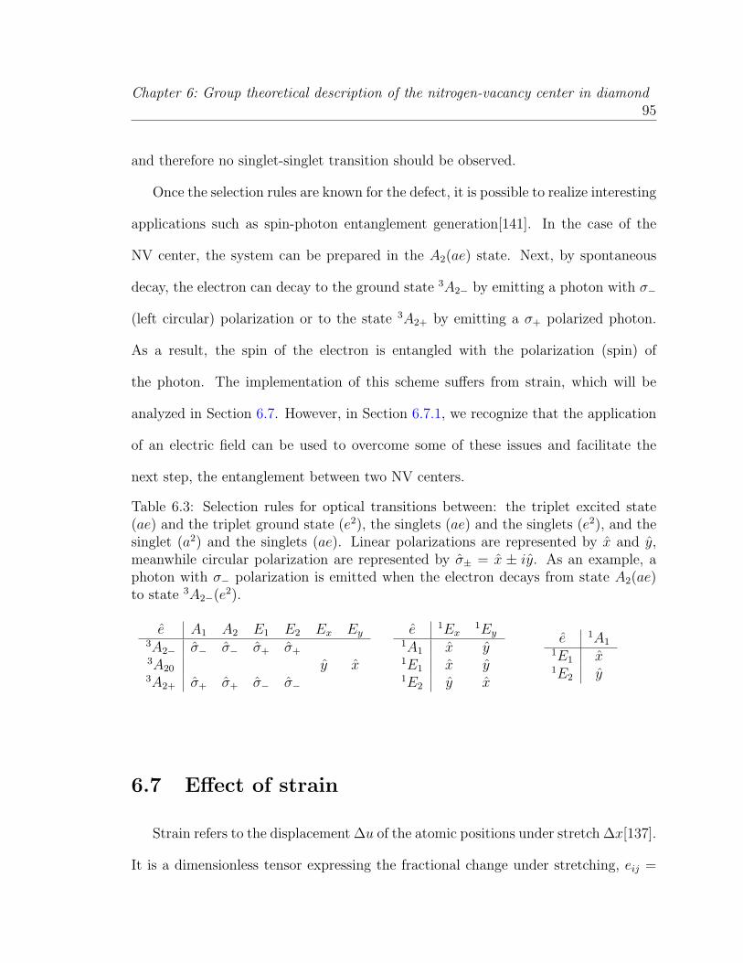
Chapter 6: Group theoretical description of the nitrogen-vacancy center in diamond95
and therefore no singlet-singlet transition should be observed.
Once the selection rules are known for the defect, it is possible to realize interesting
applications such as spin-photon entanglement generation[141]. In the case of the
NV center, the system can be prepared in the A2(ae) state. Next, by spontaneous
decay, the electron can decay to the ground state 3A2− by emitting a photon with σ−
(left circular) polarization or to the state 3A2+ by emitting a σ+ polarized photon.
As a result, the spin of the electron is entangled with the polarization (spin) of
the photon. The implementation of this scheme suffers from strain, which will be
analyzed in Section 6.7. However, in Section 6.7.1, we recognize that the application
of an electric field can be used to overcome some of these issues and facilitate the
next step, the entanglement between two NV centers.
Table 6.3: Selection rules for optical transitions between: the triplet excited state(ae) and the triplet ground state (e2), the singlets (ae) and the singlets (e2), and thesinglet (a2) and the singlets (ae). Linear polarizations are represented by x and y,meanwhile circular polarization are represented by σ± = x ± iy. As an example, aphoton with σ− polarization is emitted when the electron decays from state A2(ae)to state 3A2−(e2).
e A1 A2 E1 E2 Ex Ey3A2− σ− σ− σ+ σ+3A20 y x3A2+ σ+ σ+ σ− σ−
e 1Ex1Ey
1A1 x y1E1 x y1E2 y x
e 1A11E1 x1E2 y
6.7 Effect of strain
Strain refers to the displacement ∆u of the atomic positions under stretch ∆x[137].
It is a dimensionless tensor expressing the fractional change under stretching, eij =

Chapter 6: Group theoretical description of the nitrogen-vacancy center in diamond96
∂δRi∂xj
, and it can be produced by stress (forces applied to the solid structure), electric
field and temperature [142]. Systematic study of strain can be used to unravel the
symmetry of defects and explore their properties[143]. Strain can shift the energy
of the states as well as mix them. It reduces the symmetry of the crystal field by
displacing the atoms. However, not all nine components of strain change the defect
in a noticeable way. The antisymmetric part of eij transforms as a generator of the
rotational group and therefore only rotate the whole structure. The symmetry and
energies of the unperturbed states do not change upon rotation. Only the symmetric
part of strain, ε = e+ eT affects the structure of a defect[137]. As any other element
of the theory, strain can be expressed in terms of matrices that transform according
to the IRs of the point group under consideration. These matrices can be found by
projecting a general strain matrix on each IR,
εr =lrh
∑e
χ∗eR†eεRe. (6.11)
In Appendix E.4 we show in detail how to find the effect of strain on the eigenstates
of the defect. For simplicity, in the case of the NV center we only write the effect of
strain in the manifold ex, ey, a(1),
Σs = δaA1Aa1 + δbA1A
b1 + δaE1E
a1 + δaE2E
b2 + δaE1E
a1 + δbE2E
b2 (6.12)
where δaA1 = (exx + eyy)/2, δbA1 = ezz, δaE1 = (exx − eyy)/2, δaE2 = (exy + eyx)/2,
δbE1 = (exz + ezx)/2, δbE2 = (eyz + ezy)/2 and
Aa1 =
(1 0 0
0 1 0
0 0 0
)Ea
1 =
(1 0 0
0 −1 0
0 0 0
)Ea
2 =
(0 1 0
1 0 0
0 0 0
)(6.13)
Ab1 =
(0 0 0
0 0 0
0 0 1
)Eb
1 =
(0 0 1
0 0 0
1 0 0
)Eb
2 =
(0 0 0
0 0 1
0 1 0
),

Chapter 6: Group theoretical description of the nitrogen-vacancy center in diamond97
in the manifold ex, ey, a1(2). The effect of strain on the orbitals a1(2), ex, ey is
easy to see. Aa1 will shift equally the energies of the states ex and ey, while Ab1 will
shift the energy of states a1. Note that both are axial stresses: the former leaves
the e2 electronic configuration unaffected and the latter leaves the ea configuration
unaffected. Either one produces relative shifts between both configurations, resulting
in an inhomogeneous broadening of the optical transitions. However, they do not
change the selection rules. Only the stress Aa1 +Ab1, corresponding to either expansion
or contraction, leaves all relative energies unaffected. Eax splits the energy between ex
and ey and Eay mixes the two states. Finally, Eb
x and Eby mixes the states ex and a1 and
ey and a1, respectively. In the case of the NV center, the effect of the matrices Ebx,y
can be neglected thanks to the large gap between orbitals a1(2) and ex,y. Therefore,
in what follows we do not consider them further.
Recent work has been done to analyze how strain affects the excited state structure
of the NV center [127, 112]. Here we derive the explicit form of strain affecting the
different electronic configurations and look at two important consequences of strain
that are relevant for experiments: first, how strain affects the selection rules described
in Section 6.6 and second, how strain affects the gap among the states of the lower
branch of the triplet excited state making them vulnerable to small local perturbation.
The relevant strain matrices we will consider are Eax and Ea
y , for which the hamil-
tonian is,
Hstrain = δaE1 (|ex〉〈ex| − |ey〉〈ey|) + δbE2 (|ex〉〈ey|+ |ey〉〈ex|) . (6.14)

Chapter 6: Group theoretical description of the nitrogen-vacancy center in diamond98
This mostly affects the singlet and excited state configurations in the following form,
δx −iδy−iδy δx
δx δy
δy −δxδx iδy
iδy δx
2δx
2δy
2δx 2δy
δx δy
δy −δx,
(6.15)
for the bases A1, A2, Ex, Ey, E1, E2, 1E1,1E2,
1A1 and 1Ex,1Ey, respectively.
The ground state, due to its antisymmetric combination between ex and ey, is stable
under the perturbation Hstrain. This can be checked by applying the ground state
given in Table 6.1 to Equation (6.14). The effect on the excited state triplet can be
seen in Figure 6.3a, where the unperturbed states are mixed in such a way that, in the
limit of high strain, the excited triplet structure splits into two triplets with spatial
wavefunction Ex and Ey. When strain overcomes the spin-orbit interaction (δx > 5.5
GHz), the spin part decouples from the spatial part and total angular momentum
is no longer a good quantum number. Transitions from the excited state triplet to
the ground state triplet are linearly polarized, where the polarization indicates the
direction of strain in the xy plane.
Figure 6.3c shows how the polarization of the emitted photon from the state
A2 to the ground state 3A2−, varies from circular to linear as a function of strain.
In the case of δy strain, the effect is similar but now the mixing is different. As
shown in Figure 6.3, A2 mixes with E1 and the photons become polarized along
x − y. Note that, in the limit of low strain, in both cases the polarization remains

Chapter 6: Group theoretical description of the nitrogen-vacancy center in diamond99
! " #! #" $!
!$!
!#"
!#!
!"
!
"
#!
#"
$!
$"
%&'()*+!,+-./01
#234"+56+7+./0
8(*)9:;<+=>#?>$?@#?@$?@A?@B?C
!
"
#
$%$$
$&
! #! $!
!
!2$
!24
!2D
!2E
#
%&'()*+!F+-./01
'()*+,-."
/&
0$
! #! $!
!
!2$
!24
!2D
!2E
#
%&'()*+!F+-./G1
H:;(')G(&):*+9:'+>$+"+I>$!
.
.
)!1
)21
#!
#2
! #! $!
!
!2$
!24
!2D
!2E
#
%&'()*+!,+-./01
'()*+,-."
/&
0&
! #! $!
!
!2$
!24
!2D
!2E
#
%&'()*+!,+-./G1
H:;(')G(&):*+9:'+>$+"+I>$!
.
.
1
)
#!
#2
a) b)
c)
Figure 6.3: Excited state structure as a function of strain. a) Eigenvalues ofthe excited state triplet as a function of δx strain. b) Mixture of the eigenstate withhigher energy (corresponding to A2 in the limit of low strain) and c) the polarizationof dipolar radiation under transitions from this state to the 3A2+ state of the groundstate. Note that in both cases the circular polarization character of radiation remains.On the other hand, the linear polarization rotates 90 for strain along δy with respectto that of strain along δx.
right circularly polarized for the transition between the excited state A2(ae) to the
ground state3A2−(e2), while the polarization remains left circular for the transition
between the excited state A2(ae) to the ground state 3A2+(e2). The fact that at lower
strain the character of the polarization remains circular has been succesfully used in
entanglement schemes [124]. The polarization properties of the states Ex,y are similar
to those of the states A1,2 but with the opposite polarization.
It is important to note that the effect of external strain depends on the gap between

Chapter 6: Group theoretical description of the nitrogen-vacancy center in diamond100
! " #! #" $!
!$!
!#"
!#!
!"
!
%&'()*+,-./0
,-./0
!"
!#
$
! " #! #" $!
!
!1"
#
#1"
$
$1"
2
21"
3
%&'()*+,-./0
,-./0
!#!!"
$!!"
$!!#
! " #! #" $!
!$!
!#"
!#!
!"
!
%&'()*+,-./0
,-./0
!"
!#
$
! " #! #" $!
!
!1"
#
#1"
$
$1"
2
21"
3
%&'()*+,-./0
,-./0
!#!!"
$!!"
$!!#
! " #! #" $!
!$!
!#"
!#!
!"
!
%&'()*+,-./0
,-./0
!"
!#
$
! " #! #" $!
!
!1"
#
#1"
$
$1"
2
21"
3
%&'()*+,-./0
,-./0
!#!!"
$!!"
$!!#
! " #! #" $!
!$!
!#"
!#!
!"
!
%&'()*+,-./0
,-./0
!"
!#
$
! " #! #" $!
!
!1"
#
#1"
$
$1"
2
21"
3
%&'()*+,-./0
,-./0
!#!!"
$!!"
$!!#
! " #! #" $!
!$!
!#"
!#!
!"
!
%&'()*+,-./0
,-./0
!"
!#
$
! " #! #" $!
!
!1"
#
#1"
$
$1"
2
21"
3
%&'()*+,-./0
,-./0
!#!!"
$!!"
$!!#
! " #! #" $!
!$!
!#"
!#!
!"
!
%&'()*+,-./0
,-./0
!"
!#
$
! " #! #" $!
!
!1"
#
#1"
$
$1"
2
21"
3
%&'()*+,-./0
,-./0
!#!!"
$!!"
$!!#
a)
b)
Figure 6.4: Energy gap among states in the lower branch of the tripletexcited state under strain. a) Energy between mixtures 10 and 12 goes to zero atδx = 7 GHz as well as the difference between mixtures 9-10 at 19 GHz. For such smallgaps any external interaction involving spin might mix the states. b) In particular,an external magnetic field of 30 Gauss can mix the two states and create the observedanticrossing levels [129]. Also, the nuclear spin interaction can cause a similar effect[144].
states. As an example, we analyze the gap between states of the lower branch of the
excited state triplet under strain. On Figure 6.4, we show the gap among the states
Ex, E1, E2 as a function of strain. Notice that at δx = 7 GHz the gap between states

Chapter 6: Group theoretical description of the nitrogen-vacancy center in diamond101
Ex and E1 reduces to zero and the states cross each other. At this point any small
perturbation that mixes the states can transform this crossing into an anticrossing
point. In particular, we have shown that the spin-spin interaction can mix the states
and also the addition of an external magnetic field or the interaction with the nuclear
spin of the nitrogen [144] can cause this effect. For low magnetic field, the interaction
the most contribute to the mixing of the states and, therefore, to non-spin-preserving
transitions is the spin-spin interaction. This effect is enhanced when strain reduces the
gap between states. We emphasize that the non-axial spin-orbit interaction cannot
cause this mixing as it is invariant under C3v and it only mixes states from different
electronic configurations.
6.7.1 Strain and Electric field
The application of an electric field to a defect leads to two main effects. The first
effect, the electronic effect, consists of the polarization of the electron cloud of the
defect, and the second one, the ionic effect, consists of the relative motion of the
ions. It has been shown that both effects are indistinguishable, as they have the same
symmetry properties[145]. The ionic effect is related to the well-known piezoelectric
effect. When a crystal is under stress, a net polarization Pi = dijkσjk is induced
inside the crystal, where dijk is the third-rank piezoelectric tensor and σjk represents
the magnitude and direction of the applied force. Conversely, the application of an
electric field might induce strain given by εjk = dijkEi, where Ei are the components
of the electric field[142]. The tensor dijk transforms as the coordinates xixjxk and,
therefore, group theory can be used to establish relations between its components

Chapter 6: Group theoretical description of the nitrogen-vacancy center in diamond102
!! !"#$ " "#$ !
!%
!&
!'
!!
"
!
'
&
%
()*+,-./0*12345*6!!!7
891:;*8<=>9*+?@)0
!"#!#$%&'()*+
,-%&'()*+
!! !"#$ " "#$ !
!"#A
!"#%
!"#'
"
"#'
"#%
"#A
(B*+,-./0*12345*6'*!!*!!7
!"#!#$%&'()*+
,-%&'()*+
a) b)
Figure 6.5: Piezo electric response of optical transitions. (a) response to elec-tric fields along the NV-axis ([111] orientation or equivalents). The defect only showslinear Stark Shift independent on the initial strain. (b) electric field is applied perpen-dicular to the NV-axis in the absence of strain (solid lines). The optical transitions3A2(ms = 0) → Ex(ms = 0) and 3A2(ms = 0) → Ey(ms = 0) are split linearly andevenly. In the presence of strain along the y direction (dashed lines), the response isquadratic due to the splitting between Ex and Ey states in the excited state. Ournumerical results are in fair agreement with experimental results[146].
for a given point group. In particular, the non-zero components should transform as
the irreducible representation A1. By projecting dijk (or xixjxk) onto the irreducible
representation A1, we can determine the non-zero free parameters of the tensor d and
determine the effect of electric field on the eigenstates of the unperturbed defect (see
Appendix E.4). In the case of the NV center, the effect on the excited state triplet is
given by following matrix,

Chapter 6: Group theoretical description of the nitrogen-vacancy center in diamond103
HE = (b+ d)Ez + a
Ex −iEy−iEy Ex
Ex Ey
Ey −ExEx iEy
iEy Ex
, (6.16)
in the basis A1, A2, Ex, Ey, E1, E2, while the effect on the ground state triplet is
HE = 2bEz, (6.17)
in the basis 3A2+,3A20,
3A2−. Comparing Equations (6.16) and (6.17), we note that
the linear response of the excited state and ground state are in principle different.
The use of an electric field along the z (NV-axis) can be used to tune the optical
transition without distorting the C3v symmetry of the defect, provided b 6= d. In
Figure 6.5a we show the linear response of NV centers under electric field parallel
to the NV-axis. In this case, the linearity is not affected by the presence of strain.
Our estimations for the ionic effect, based on the response of the lattice defect to
electric field and the response of the orbital energies to strain (see Appendix E.4),
indicate that the relative shift between the ground and excited state is about 2 GHz
/ MV/m. This could be very important to entangle two NV centers optically as the
wavelength of the photons emitted from each NV center need to overlap[Reference
here]. In addition, an electric field with components Ex,y can be used to completely
restore the C3v character of the defect. In Figure 6.5b, we show the response of
optical transitions under an electric field perpendicular to the NV axis. In this case,

Chapter 6: Group theoretical description of the nitrogen-vacancy center in diamond104
the response is linear if strain is absent and quadratic if strain is non-zero. Dashed
lines show the response to a 0.5 GHz strain along the [01-1] axis.
6.8 Conclusions
We have used group theory to identify, analyze and predict the properties of NV
centers. This analysis can be extended to deep defects in solids. A careful analysis of
the properties of a defect via group theory is essential for realization of spin-photon
entanglement generation and to control the properties of NV centers such as undesired
strain. We have shown that group theoretical approaches can be applied to determine
the ordering of the singlets in the (e2) electronic configuration and to understand the
effect of spin-orbit, spin-spin and strain interactions.

Chapter 7
Conclusions and Outlook
Control over individual NV centers have enabled us to understand many aspects of
many body dynamics associated with solid-state environments. The ability to explore
individual centers by confocal microscopy provides a great amount of information, not
only on how the center can coherently interact with its nearby environment, but also
on how aggregation of individual NV systems build up the signal from ensemble
measurements[68, 32]. It is also now well understood how important it is to have
control of the isotopic composition of the diamond lattice. Reducing the concentration
of Nitrogen impurities and Carbon-13 greatly improves the coherence times of the NV
electronic spin[104] and therefore the performance of a number of applications: e.g.,
recall that NV magnetic field sensitivity scales inversely proportional to the coherence
time, T−12 , see Chapter 3. Thus a future challenge is to increase the number of sensing
NV defects without increasing the number of Nitrogen impurities,which can provide
the means for NV spin decoherence. Finding the right balance of NV concentration is
crucial to enable high sensitivity magnetometry using large numbers of sensing spins.
105

Chapter 7: Conclusions and Outlook 106
In the case of shallow implanted defects, there is still much to understand about
how they interact with impurities or localized states at the surface of the material,
which seem to rapidly decohere the NV electronic spin. It is crucial to control these
undesired effects to employ NV centers as feasible candidates for short distance (∼
10 nm) spin detection and magnetic imaging of biological samples.
Magnetic sensing combined with the high spatial resolution technique presented
in Chapter 5 may have many interesting applications. For example, NV centers
could be used to directly image the activity of neuronal networks, or map the local
concentration in living cells of paramagnetic molecules such as nitric oxide (NO) and
other reactive oxygen species. Our spin-RESOLFT technique is particularly useful
for biological samples as it uses considerable less laser power than conventional STED
techniques and therefore should be less harmful to living cells.
Although we generally think of nuclear spins (primarily Carbon-13 in diamond)
as impurities that cause NV spin-decoherence, we have seen in Chapter 4 that nearby
nuclear spins are not always harmful to NV properties when they can be isolated from
their environment[39]. Our results show that NV centers in diamond can effectively
implement useful quantum control algorithms in solid-state systems by manipulating
several nuclear spins proximal to an NV center. In addition, we showed that NV
centers can be used for coherent non-destructive mapping of states from other quan-
tum systems such as nearby nuclear spins or electronic spins. This property may
be combined with transport of nanocrystals on cantilevers[46], enabling a powerful
tool for quantum information transport or with high spatial resolution and coherent
control (see Chapter 5) of an array of NV centers. The latter modality may be a
Chapter 7: Conclusions and Outlook 107
feasible way to realize room temperature quantum computation in which an array of
NV centers separated by 10-30 nm from each other can coherently interact via spin
dipole-dipole to enable high fidelity two-qubit operations. The nuclear spin of the
NV center can then serve as a qubit memory that can be addressed individually by
using the spin-RESOLFT technique.
The stability of a defect is determined by how the level structure of the defect
behaves under perturbations such as vibrations and crystal deformation. As an ex-
ample, the ground state of the negatively charged NV center is stable under static
Jahn-Teller distortions of the lattice[147] because it has the two degenerate energy
levels are fully occupied. Many of these properties/characteristics are well under-
stood when the problem is approached from group theory. In fact, in the case of the
NV center the crystal field produces a robust excited state for spin-photon entangle-
ment schemes (see Chapter 6) thanks to how the crystal field sets the way spin-spin
and spin-orbit interactions manifest. Looking at the symmetry of the crystal field
not only successfully predicts this behavior but also provide the tools to analyze the
performance of this scheme under perturbations that reduce the symmetry. In this
regard, there is still much work to do to understand how the different vibrations are
coupled to the defect. An accurate group theoretical analysis can be used to predict
the properties of other centers and more importantly engineer defects with desired
properties.
We have seen that the properties of nitrogen-vacancy centers have enabled a num-
ber of interesting applications that exploit the quantum manipulation of spin and
Chapter 7: Conclusions and Outlook 108
orbital degrees of freedom. Many of these applications, such as magnetic sensing,
are just starting to become efficient; and although there is still much to understand
about the complex structure of this center and its environment, the community has
gained a great deal of experience and at the same time been surprised about the NV
center’s outstanding properties at room temperature, enabled by symmetry and by
the large band gap of diamond. Present technology has enabled researchers to explore
in exquisite detail the structure and environment of the NV center, though there is
still work to do and perhaps surprises awaiting in the ultra fast dynamics of the NV
center. Finally, the fortuitous properties of the NV center might not be unique to
it. We should also be open to explore not only other types of point defects but also
delocalized ones, where an ensemble of quantum degrees of freedom might join to
build a robust quantum manifold.

Appendix A
Supporting material for Chapter 2
A.1 Phenomenological models for decoherence
When the details of the interaction between the central spin and the environment
and the properties of the latter are not known or difficult to model, the effect of the
environment on the central spin can be model by a random fluctuating field b(t) with
mean value zero and some spectral density Sb(ω). In the case of the NV center, the
relevant hamiltonian for this approach is
H = ∆S2z +B · S + b · S (A.1)
where ∆ is the zero field splitting, B is the static external magnetic field. To second
order perturbation theory (see Section A.4 in this Appendix), hamiltonian (A.1) can
be written as
H = ∆S2z +B · S + bzSz +
∑m
|m〉〈m| (αmb⊥ + βmb2⊥)
(A.2)
109

Appendix A: Supporting material for Chapter 2 110
where αm = (3m2− 2)B⊥/2∆ and βm = (3m2− 2)/∆. The free induction decay (fid)
and echo signals of an initial state ϕi = |a〉+ |b〉 is proportional to
p =1
2+
1
2exp
(−〈Φ2〉/2) (A.3)
where ∆φ = δφ(0, τ) and ∆φ = δφ(−τ/2, 0) − δφ(0, τ/2), respectively. δφ(t1, t2) =
φa(t1, t2) − φb(t1, t2) and φm(t1, t2) =∫ t2t1dt〈m|H/~|m〉. It is clear from Equation
(A.2) that there will be a dependence on the angle θ between the NV axis and the
magnetic field. However, in this section, our aim is not to study this dependence but
the effect of the environment via the stochastic variable b. Therefore, in what follows
we will neglect the angular dependence and consider only,
φm(t1, t2) = m
∫ t2
t1
b(t)dt (A.4)
For φ(t1, t2) =∫ t2t1b(t)dt and b a random variable, it can be shown that
〈Φ2〉fid =2
π
∫ ∞0
dωSb(ω)
ω2sin2
(ωτ2
)〈Φ2〉echo =
8
π
∫ ∞0
dωSb(ω)
ω2sin4
(ωτ4
)(A.5)
and Sb(ω) is the spectral density which is characterize by the average power P of
the random field, P = 12π
∫∞0Sb(ω)dω = 1
T
∫∞−∞〈xT (t)2〉dt.
Table A.1: Various types of spectral densities and its corresponding echo decay. Thespectral density is given by Sb(ω) between the range of frequencies ωa and ωb and 0otherwise.
Noise Sb(ω)/NP N 〈Φ2〉echo/2NPWhite 1 2π
(ωb−ωa)14τ
1/f ω−1 2πlog(ωb/ωa)
log(2)4π
τ 2
1/f 2 ω−2 2πωaωb(ωb−ωa)
124τ 3

Appendix A: Supporting material for Chapter 2 111
Spectral densities that transform as ω−n are not realistic for low frequencies.
Instead, many experiments show a constant spectral density for frequencies between
0 and some particular cut-off ωc[148]. For frequencies above this cut-off, the spectral
density can be modeled by the spectral densities given in Table A.1. In most of the
cases, this constant part of the spectral density leads to decoherence in fid signals
giving the characteristic decay exp (−τ 2). In these cases, ωτ 1 for the relevant
frequencies that contributes to the decay. On the other hand, in cases where the
large frequency components contributes as much as the low frequencies, the fid signal
decays exponentially, exp (−τ), revealing an environment with a fast dynamics.
For these reasons, a lorentzian spectral density is used to model both, fid and echo
decays,
Sb(ω) =Pτc
1 + ω2τ 2c
(A.6)
where τc is the correlation time of the environment,
〈b(τ + t)b(t)〉 = P exp (−τ/τc) (A.7)
For times τ ≤ τc, we find that the signal is given by,
pfid =1
2
(1 + exp− (τ/T ∗2 )2) pfid =
1
2
(1 + exp− (τ/T2)4) (A.8)
where T ∗2 =√
2/P , T2 = (2τ 2c /αP )
1/4and α = (4−π)/2π. Leading to the well-known
relation,
T2 =√
1.6τcT ∗2 . (A.9)

Appendix A: Supporting material for Chapter 2 112
A.2 Decoherence due to off-axis magnetic field
When the magnetic field is not aligned with the NV axis, the electronic spin echo
signal decoheres. This effect is solely due to the interaction between the central spin
and the bath of nuclear spins and not due to the interaction among spins in the
bath. As explained in Chapter 2, revivals occur because all nuclei precess with the
same frequency when the electron is in its 0 state. If only one nucleus precess at a
different rate, the center decoheres. In this section we will analyze the form of this
decoherence. The contribution to the echo signal of one nucleus is
Sn(τ) = 1− 2|Ω0 × Ω1|2 sin2 Ωn0τ
2sin2 Ω1τ
2. (A.10)
The Larmor frequency of a single nucleus can be enhanced by the electron due to
virtual process (see Section A.4 in this Appendix) and therefore the nucleus might
precess at a different rate rather than at the bare Larmor frequency Ω0, i.e., Ωn0 =
Ω0 + δΩn0 . At the revivals we have that sin Ωτ/2 = 0 and consequently,
sinΩn
0τ
2= sin
(Ω0 + δΩn0 ) τ
2= sin
Ω0τ
2cos
δΩn0τ
2+ sin
δΩn0τ
2cos
Ω0τ
2
= sinδΩn
0τ
2(A.11)
Therefore, the pseudo spin at the revivals is given by
Senvn (τ) = 1− 2|Ω0 × Ω1|2 sin2 δΩ
n0τ
2sin2 Ω1τ
2(A.12)
If now we consider that δΩ0 is small and Ω1 is large we can do the following approx-
imations
sin2 δΩn0τ
2≈ δΩn2
0 τ2
4sin2 Ω1τ
2≈ 1
2, (A.13)

Appendix A: Supporting material for Chapter 2 113
which leads to the following envelope for the echo signal
Senvn (τ) ≈ 1− |Ω0 × Ω1|2 δΩ
n20 τ
2
4. (A.14)
In addition, it is not difficult to see that to leading order in θ (the angle between the
NV axis and the magnetic field), δΩn0 ∝ θ. At this point we can approximate the
signal by
Soff-axisenv (τ) ≈ exp
(−αθ2τ 2). (A.15)
The envelope now decays as a Gaussian.
A.3 Ensemble measurements
It is found that on ensemble measurements the decay of the echo signal does not
follow the predicted decay of single defects (exp (−τn) with n = 3− 4). Instead,
the signal falls off with lower n’s looking even exponential. In dilute samples, where
average distance between NV centers is large enough so that the interaction between
them is neglected, this effect is just the average of many single echo signals with
different decay rates. As explained in Chapter 2, when the magnetic field is off axis,
the ensemble signal is the average of many gaussian decays with different rates,
E(τ) =
∫f(b) exp
(−bτ 2)db. (A.16)
In this section, we show that the distribution for the parameter b is f(b) = b−3/2.
It is clear from Section A.2 that the parameter b in Equation (A.16) is proportional
to the hyperfine interaction squared between the central spin and the nearby nucleus

Appendix A: Supporting material for Chapter 2 114
n,
b = A2n =
(µ0
4πγeγn
)2 1
r6(A.17)
where r is the distance between the central spin and nucleus n. On a cubic lattice, this
distance is given by r2 = a2 (i2 + j2 + k2) where a is the nearest neighbor distance
and i, j, k are indices running from −I to I. The position i = j = k = 0 is
excluded since it correspond to the position of the central spin. The distribution
for the distance is clearly fr(r) = 4πr2. And the distribution for the variable b can
be calculated following recipes from statistical analysis as follow. The cumulative
probability distribution for the variable b is given by
Fb(b) =
∫b≤r−6
fr(r)dr ∝ r3|rmaxb−1/6 = cte− b−1/2 (A.18)
and therefore,
fb(b) =∂Fb(b)
∂b= b−3/2, (A.19)
which needs to satisfy∫f(b) = 1. b can vary between
bmin =(µ0
4πγeγn
)2 1
r6max
bmax =(µ0
4πγeγn
)2 1
a6(A.20)
and therefore the normalized distribution is
fb(b) = 2b−3/2
(1√bmin
− 1√bmax
). (A.21)
A.4 Non-Secular Correction
The most common approximation in central spin problems is the so called secular
approximation which consists on neglecting off diagonal elements of the central spin
Appendix A: Supporting material for Chapter 2 115
manifold. However, experiments have proven that this approximation is not enough
to account for all observations. A clear example is the Knight shift. Also observed is
the enhanced coupling between two other spins that interact via virtual transitions
with the central spin. All this phenomena can be explained by perturbation theory.
In this appendix we work in detail the perturbation contribution of non-secular terms
to the dynamics of the nuclear bath for a central spin 1 (NV case) and for a central
spin 1/2.
Elements of perturbation theory
Consider the hamiltonian of a central spin S in the presence of a nuclear spin bath
In,
H = ∆S2z − γeB · S−
∑n
γnB · In −∑n
S ·An · In −∑n>m
In ·Cnm · Im (A.22)
or
H = ∆S2z − γeB · S−
∑n
γnB · In −∑n,i,j
SiAnijI
nj −
∑n>m,i,j
Ini Cnmij Imj
where the index n runs over the nuclear bath, i, j = x, y, z. The first term is the zero
field splitting only relevant when S > 12, the second and third term are the Zeeman
interactions for the central spin and nuclear bath, respectively, the fourth term is
the hyperfine interaction between the central spin and the nuclear bath and the last
term is the dipole-dipole interaction among nuclear spins. In order to approach this
problem perturbatively, we identify the secular H0 and non-secular V part of the
hamilonian,

Appendix A: Supporting material for Chapter 2 116
H0 = ∆S2z − γeBzSz −
∑n γNB · In −
∑nj SzA
nzjI
nj , (A.23)
the non-secular one, which will be treated as a perturbation,
V = −12
(γe (B−S+ +B+S−) +
∑nj
(S+A
n−jI
nj + S−A
n+jI
nj
)). (A.24)
The hamiltonian of the nuclear bath will not be relevant for the purpose of this
appendix,
Hnuc = −∑n>m
In ·Cnm · Im. (A.25)
Second order perturbation theory states that[149],
E(2)i = 〈φi|V Q 1
E(0)i −H0
QV |φi〉 (A.26)
where |φ〉 is the unperturbed state manifold of the central spin, Q = 1 − P and
P = |φi〉〈φi|.
Perturbation for S = 1 central spin
For the case of S = 1 we have that to second order the corrections for the energies
are
E(2)±1 =
〈±1|V |0〉〈0|V |±1〉E
(0)±1 − E(0)
0
(A.27)
E(2)0 =
〈0|V |−1〉〈−1|V |0〉E
(0)0 − E(0)
−1
+〈0|V |1〉〈1|V |0〉E
(0)0 − E(0)
1
(A.28)
where E(0)0 − E(0)
±1 = −∆± γeBz and
〈0|V |±〉 = − 1√2
(γeB± +
∑n
A±n · In)
(A.29)
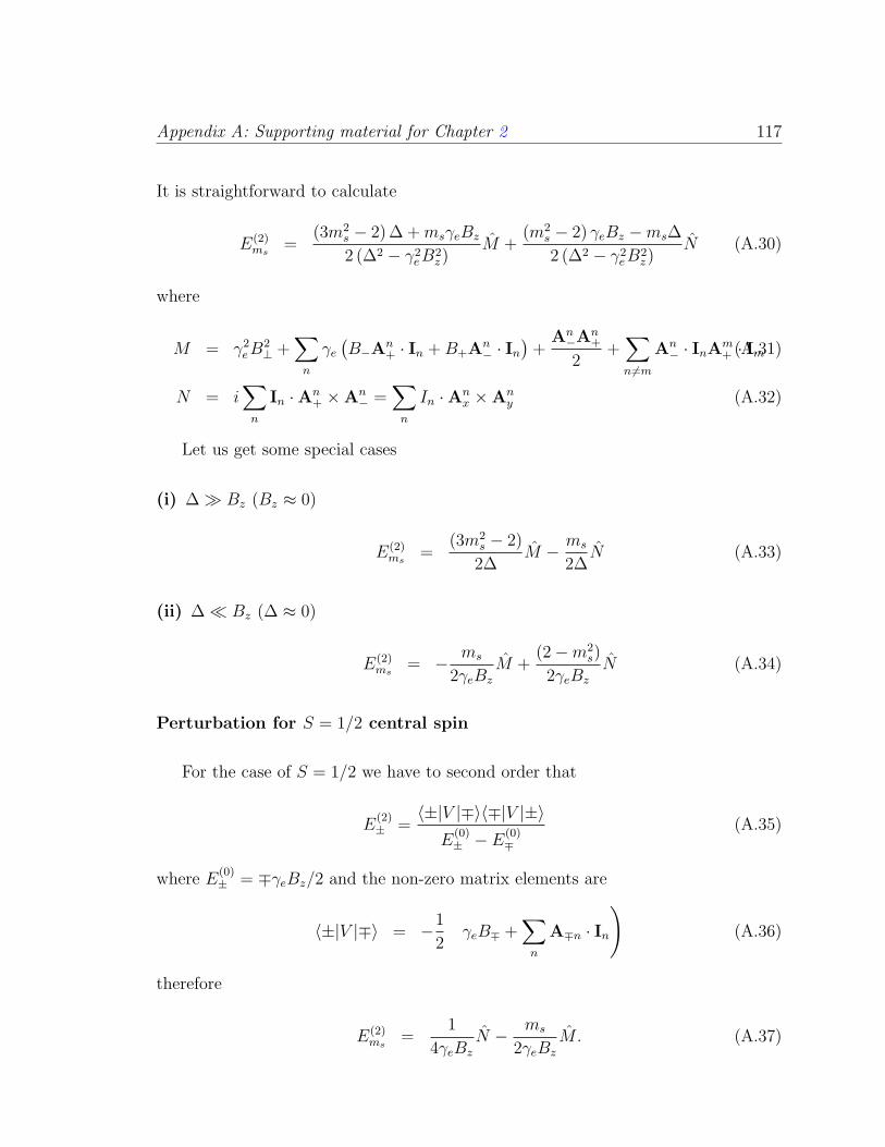
Appendix A: Supporting material for Chapter 2 117
It is straightforward to calculate
E(2)ms =
(3m2s − 2) ∆ +msγeBz
2 (∆2 − γ2eB
2z )
M +(m2
s − 2) γeBz −ms∆
2 (∆2 − γ2eB
2z )
N (A.30)
where
M = γ2eB
2⊥ +
∑n
γe(B−An
+ · In +B+An− · In
)+
An−An
+
2+∑n 6=m
An− · InAm
+ · Im(A.31)
N = i∑n
In ·An+ ×An
− =∑n
In ·Anx ×An
y (A.32)
Let us get some special cases
(i) ∆ Bz (Bz ≈ 0)
E(2)ms =
(3m2s − 2)
2∆M − ms
2∆N (A.33)
(ii) ∆ Bz (∆ ≈ 0)
E(2)ms = − ms
2γeBz
M +(2−m2
s)
2γeBz
N (A.34)
Perturbation for S = 1/2 central spin
For the case of S = 1/2 we have to second order that
E(2)± =
〈±|V |∓〉〈∓|V |±〉E
(0)± − E(0)
∓(A.35)
where E(0)± = ∓γeBz/2 and the non-zero matrix elements are
〈±|V |∓〉 = −1
2
(γeB∓ +
∑n
A∓n · In)
(A.36)
therefore
E(2)ms =
1
4γeBz
N − ms
2γeBz
M. (A.37)

Appendix A: Supporting material for Chapter 2 118
Back action on nuclear bath
The above analysis found new terms for the dynamics of the nuclear bath which
now we will put in more familiar terms. First we need to distinguish between constant
terms and dynamics terms, terms that depend on the state of the nucleus. The M
operator contains a constant part MC and a dynamic part MD,
M = MC + MD (A.38)
MC = γ2eB
2⊥ +
1
2
∑n
|Anx|2 + |An
y |2 (A.39)
MD =∑n
2γeB ·Gn · In +∑n>m
2In ·GTnGm · Im (A.40)
where
Gn =
Anx
Any
0
=
Anxx Anxy Anxz
Anyx Anyy Anyz
0 0 0
(A.41)
meanwhile
N =∑n
In · Fn (A.42)
is purely dynamic and
Fn = Anx ×An
y =
AxyAyz − AyyAxzAyxAxz − AxxAyzAxxAyy − AyxAxy
(A.43)
As an example, we write the case of the NV center for low field,
E(2)ms =
∑n
B · (3m2s − 2
) γe∆
Gn · In − In ·ms1
2∆Fn
+(3m2
s − 2)
∆
∑n>m
In ·GTnGm · Im (A.44)

Appendix A: Supporting material for Chapter 2 119
where the first term can be thought as an enhanced g-tensor
∆gn =(3m2
s − 2) γeγn∆
Gn (A.45)
Depending on the system under consideration the hyperfine interaction can be purely
contact interaction as it is the case of quantum dots o purely dipolar as it would
be the case for far enough nuclei in deep centers (where the wavefunction is very
localized). Therefore, it is instructive to know the form of these matrices for these
special cases. In the case of a purely contact interaction Aij = aδij we have,
Gn =
a
a
0
Fn =
0
0
a2
GTnGm =
anam
anam
0
(A.46)
Meanwhile the purely dipolar case is pretty much filled everywhere.
Effective g-tensor
One of the consequences of this correction is an enhanced coupling between nuclei
spins and the external magnetic field, which can be expressed in terms of an effective
g-factor
gn (ms)ij = gcδij − (3|ms| − 2)gcγe
2∆γN(1− δiz)Anij (A.47)
or
gn (ms)ij = gcδij + ∆gn (ms)ij (A.48)
where
∆gn (ms)ij = − (3|ms| − 2) gcγe2∆γN
(1− δiz) (anδij + bn (δij − 3rirj)) (A.49)

Appendix A: Supporting material for Chapter 2 120
where an and bn are the Fermi-contact and dipole-dipole term from the hyperfine
interaction between the electronic spin state and the nuclear spin n.
Larmor frequency and Larmor vector
Besides the coupling between the external field and the nuclear spin operator, the
latter also experiences an itself interaction mediated by the electronic spin. Both
effects modify the Larmor frequency and the direction at which the nuclear spin
precess. From Equations (A.30) and (A.31) we identify the complete effective coupling
with the nuclear spin n as
−∑ij
µNgn (mS)ij BiInj −ms (2∆)−1
∑ijk
εijkAnxiA
nyjI
nk (A.50)
and including the rest of the couplings with the nuclear spin coming from (A.23), we
can identify the following effective Larmor vector
Ωn (ms)k = −∑i
µNgn (ms)ikBi − ms
2∆
∑ij
εijkAnxiA
nyj −msA
nzk. (A.51)
This last equation tell us that each spin n has a particular Larmor frequency pointing
in a particular direction. This will be very important when analyzing the nuclear
decay. Corrections to the Larmor frequency decays exponentially and as r−3 and r−6.

Appendix A: Supporting material for Chapter 2 121
To see this result more clearly, let us analyze the case ms = 0,
Ωn (ms = 0)j = −∑i
µNgn (ms = 0)ij Bi (A.52)
= −∑i
µN
(gcδij +
gcγe∆γN
(1− δiz)Aij)Bi (A.53)
Ωn = −µN
Bx
By
Bz
−γe∆
AxxBx + AyxBy
AxyBx + AyyBy
AxzBx + AyzBy
. (A.54)
Effective Nuclear Spin Interaction
Finally, the non-secular correction leads to an effective interaction between nuclei.
From equations (A.30) and (A.31) we have that
(∆Cnm)ij =(3m2
s − 2)
2∆
∑n6=mij
(AnxiA
mxj + AnyiA
myj
)Ini I
mj . (A.55)
which can be written as a function of the correction to the g factor (∆gn)ij,
(∆Cnm)ij =1
2∆ (3|ms| − 2)
(∆γNgcγe
)2∑k
(∆gTn
)ik
(∆gm)kj . (A.56)
The pre-factor before the summation has dimension of Hz and an approximate value
of (in the case ms = 0)
1
4∆
(∆γNgcγe
)2
∼ 1
12kHz (A.57)
This constitute an important correction to the bare nuclei interaction, which is of
the order of 2 kHz for nearest neighbors. Besides this important enhancement, the
correction ∆Cnm does not depend on the relative position between nuclei, it depends
on the relative positions between the electron and each nucleus. For nearest neighbor

Appendix A: Supporting material for Chapter 2 122
nuclear spins right beside the defect, this new interaction is 1000 times grater than
the bare interaction between them, however it decreases exponentially as the nuclear
spins get away from the defect.

Appendix B
Supporting material for Chapter 3
B.1 Samples
AC magnetometry was performed at room temperature on nitrogen-vacancy (NV)
centers in both a bulk single-crystal diamond sample (1mm x 1mm x 0.5mm, natural
diamond with an atypically low nitrogen concentration) and in diamond nanocrystals
(monocrystalline, synthetic diamonds, 30 nm mean diameter, purchased from Micro-
diamant AG, www.microdiamant.com, Switzerland) deposited on a quartz coverslip
(see Figure B.1).
B.2 Confocal Setup
Single NV centers were isolated and probed via confocal microscopy (see Figure
B.2). Phonon-mediated fluorescent emission ( 630 nm - 750 nm) was detected un-
der coherent optical excitation (λ = 532 nm) using a single photon counting module
123
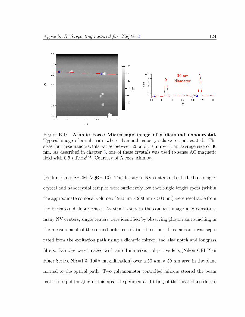
Appendix B: Supporting material for Chapter 3 124
30 nm
diameter
Figure B.1: Atomic Force Microscope image of a diamond nanocrystal.Typical image of a substrate where diamond nanocrystals were spin coated. Thesizes for these nanocrsytals varies between 20 and 50 nm with an average size of 30nm. As described in chapter 3, one of these crystals was used to sense AC magneticfield with 0.5 µT/Hz1/2. Courtesy of Alexey Akimov.
(Perkin-Elmer SPCM-AQRH-13). The density of NV centers in both the bulk single-
crystal and nanocrystal samples were sufficiently low that single bright spots (within
the approximate confocal volume of 200 nm x 200 nm x 500 nm) were resolvable from
the background fluorescence. As single spots in the confocal image may constitute
many NV centers, single centers were identified by observing photon anitbunching in
the measurement of the second-order correlation function. This emission was sepa-
rated from the excitation path using a dichroic mirror, and also notch and longpass
filters. Samples were imaged with an oil immersion objective lens (Nikon CFI Plan
Fluor Series, NA=1.3, 100× magnification) over a 50 µm × 50 µm area in the plane
normal to the optical path. Two galvanometer controlled mirrors steered the beam
path for rapid imaging of this area. Experimental drifting of the focal plane due to

Appendix B: Supporting material for Chapter 3 125
Confocal setup for NV centers
APD
Green telescope
Red telescope
Fiber coupler 1
Fiber coupler 2Filters
Dichroic
Mirror
Objective
Piezo
Red Fiber
Green Fiber
From switch box
Box
HWP
Figure B.2: Schematic of a confocal setup for NV centers. As explained inthis appendix, an NV center is excited with green line on the absorption phonon sideband and fluoresces in the range 637-800 nm. The green laser is delivered to the setupby a fiber coupler. A telescope is used so that the beam diameter of the green lasermatches the aperture of the back of the objective in order to achieve an optimumresolution. An oil immersed objective with a numerical aperture of 1.3 is used toachieve ∼250 nm resolution which is nearly diffraction limited (∼ λ/2NA). Beforereaching the objective, the green laser bounces a dichroic which reflects the green buttransmits the red light. In this way, only the fluorescence of the NV center passesthrough the dichroic and reaches a black box where photons are counted. A set offilters inside the box can be used to narrow the fluorescence bandwidth to eliminatedundesired light coming from the surface of the diamond, other impurities and evensmall green leakages. A telescope and a fiber coupler is used to better collect thefluorescence. Finally, the fiber is connected to a avalanche photon detector producinga TTL pulse that can be used to feed a counter.
thermal effects was compensated for using closed-loop feedback of the galvanometer
and objective piezo voltages. Green laser pulses were generated using an acousto-optic
modulator as shown on Figure B.3.
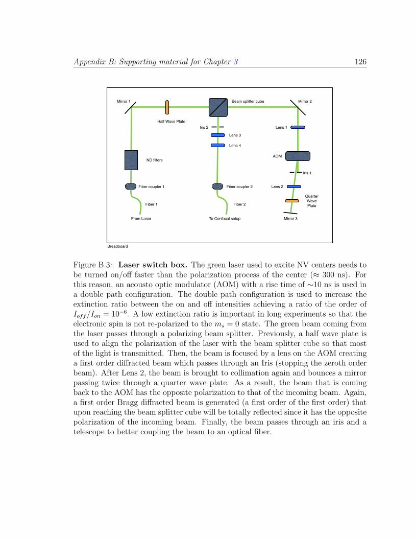
Appendix B: Supporting material for Chapter 3 126
Switch box
From Laser To Confocal setup Mirror 3
Mirror 2Mirror 1 Beam splitter cube
Lens 1
Lens 2
Quarter
Wave
Plate
AOM
Iris 2
Iris 1
Fiber coupler 2Fiber coupler 1
Half Wave Plate
Fiber 1 Fiber 2
Lens 3
Lens 4
ND filters
Breadboard
Figure B.3: Laser switch box. The green laser used to excite NV centers needs tobe turned on/off faster than the polarization process of the center (≈ 300 ns). Forthis reason, an acousto optic modulator (AOM) with a rise time of ∼10 ns is used ina double path configuration. The double path configuration is used to increase theextinction ratio between the on and off intensities achieving a ratio of the order ofIoff/Ion = 10−6. A low extinction ratio is important in long experiments so that theelectronic spin is not re-polarized to the ms = 0 state. The green beam coming fromthe laser passes through a polarizing beam splitter. Previously, a half wave plate isused to align the polarization of the laser with the beam splitter cube so that mostof the light is transmitted. Then, the beam is focused by a lens on the AOM creatinga first order diffracted beam which passes through an Iris (stopping the zeroth orderbeam). After Lens 2, the beam is brought to collimation again and bounces a mirrorpassing twice through a quarter wave plate. As a result, the beam that is comingback to the AOM has the opposite polarization to that of the incoming beam. Again,a first order Bragg diffracted beam is generated (a first order of the first order) thatupon reaching the beam splitter cube will be totally reflected since it has the oppositepolarization of the incoming beam. Finally, the beam passes through an iris and atelescope to better coupling the beam to an optical fiber.
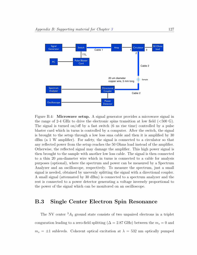
Appendix B: Supporting material for Chapter 3 127Microwaves
Signal Generator
Switch
TTL
Amp Circulator50 Ohms
load
Power Detector
Directional Coupler
Oscilloscope
Spectrum Analyzer
Pulse Blaster Card
PC
Cable 1
Cable 2
Cable 2
20 um diameter
copper wire, 5 mm long
1
2
3
Sample
Figure B.4: Microwave setup. A signal generator provides a microwave signal inthe range of 2-4 GHz to drive the electronic spins transition at low field (<500 G).The signal is turned on/off by a fast switch (6 ns rise time) controlled by a pulseblaster card which in turns is controlled by a computer. After the switch, the signalis brought to the setup through a low loss sma cable and then it is amplified by 30dBm (a 1 W amplifier). For safety, the signal is connected to a circulator so thatany reflected power from the setup reaches the 50 Ohms load instead of the amplifier.Otherwise, the reflected signal may damage the amplifier. This high power signal isthen brought to the sample with another low loss cable. The signal is then connectedto a thin 20 µm-diameter wire which in turns is connected to a cable for analysispurposes (optional), where the spectrum and power can be measured by a SpectrumAnalyzer and an oscilloscope, respectively. To measure the spectrum, just a smallsignal is needed, obtained by unevenly splitting the signal with a directional coupler.A small signal (attenuated by 30 dBm) is connected to a spectrum analyzer and therest is connected to a power detector generating a voltage inversely proportional tothe power of the signal which can be monitored on an oscilloscope.
B.3 Single Center Electron Spin Resonance
The NV center 3A2 ground state consists of two unpaired electrons in a triplet
conguration leading to a zero-field splitting (∆ = 2.87 GHz) between the ms = 0 and
ms = ±1 sublevels. Coherent optical excitation at λ = 532 nm optically pumped

Appendix B: Supporting material for Chapter 3 128
the ground state into its ms = 0 sublevel. In addition, an external static magnetic
field produced by a pair of Helmholtz coils split the degeneracy between the ms = ±1
states. It was then possible to selectively address transitions between the ms = 0 and
ms = 1 (or ms = −1) states with microwave radiation (see Figure 3.1) and manip-
ulate a two-level subspace of the spin triplet (e.g., with spin-echo pulse sequences).
Microwave radiation was applied by using the magnetic field emanating from a 20
µm wire placed on the surface of the samples.
The excited (3E) state decay rates, also responsible for optical pumping, provided
a means for spin-sensitive detection, as the rate of fluorescence was reduced for the
ms = ±1 states compared to the ms = 0 states, with > 35% contrast. The spin
state in the ground electronic state was measured by pulsing on green excitation and
monitoring the total number of photons collected within the optimal measurement
interval, 324 ns. A 300 MHz PulseBlasterESR pulse generator was employed for
timing the triggering of counters, microwave pulses, the AC magnetic field, and the
excitation laser. Microwave pulses were provided by gating the output of a frequency
synthesizer with a microwave switch (see Figure B.3). The π and π/2 pulses used for
the spin-echo sequence were calibrated from the Rabi nutation curves between the
two spin states.
B.4 AC magnetometry
As described in Figure 3.2 and in Ref. [25], demonstration magnetometer mea-
surements were performed for an externally applied AC magnetic field with amplitude
BAC , frequency ν, and phase φAC during a cycle of a spin-echo sequence with a period

Appendix B: Supporting material for Chapter 3 129
τ . The accumulated phase of the spin superposition state,
δφ =4γBAC
2πνsin2[
πντ
2] cos[πντ + φAC ] (B.1)
contained information about the projection of the AC magnetic field amplitude onto
the quantization axis of the electronic spin, corresponding to a vector magnetometer.
Oscillatory magnetic fields from 1-10 kHz were generated by modulating the current
through a Helmholtz pair also used to apply a bias DC magnetic field. For application
of higher frequency AC fields (100-300 kHz), a single coil (60 turns) was resonantly
driven and placed near the sample.
The measured signal intensity SB was a function of the accumulated phase δφ, as
given by the probability to be in the ms = 0 state after the spin-echo pulse sequence:
SB ∝ P0(BAC) = 12
(1 + F (τ) cos[δφ]). Ideally, for a single-shot measurement of BAC
the sensitivity was maximized for a particular ν by setting τ = 1/ν. In practice, many
spin-echo cycles were averaged to reduce the uncertainty in photon statistics given
the low single-shot count rate. To this end, the period of the entire measurement
sequence (including polarization and readout, see Figure 3.2) was matched to 1/ν in
order to avoid multiple offset phases φAC when the periods were incommensurate.
The dependence on φAC was removed entirely by appropriately shifting the time
origin of the measurement pulse train. As the polarization (τp = 1 µs) and readout
(τr = 3 µs) periods were short compared to the oscillation periods for typical 1-10
kHz AC magnetic fields, this choice introduced a slight deviation ε from the optimal
δφ, as τp + τr + τ = 1/ν ⇒ τν = 1 − ε. The overall sensitivity was thus slightly
reduced from its optimal value as 1 − O(ε2). For all experiments presented here,
ντ = 0.88 was used. The envelope of the spin-echo signal, F (τ) (e.g., see Figure 3.4)

Appendix B: Supporting material for Chapter 3 130
was modeled with an exponential decay modulated by the effect of a pair of nearby
strongly interacting 13C nuclear spins. In this model[85], F (τ) = exp(−(τ/T2)4)(1−(a2−b2)a2 sin2 aτ sin2 bτ); where for the data in Figure 3.4 we found T2 = 676 µs, b = 478
Hz (corresponding to the dipolar interaction between the two nuclei) and a = 626 Hz
(corresponding to the interactions between the nuclei and the NV spin). Using these
experimentally determined parameters, the above model provided a prediction for
the the magnetometer sensitivity[25] ηAC = π~gµBC
√νF (1/ν)
as a function of frequency
(solid curve in Figure 3.6a), where g ≈ 2 is the electron g-factor, µB is the Bohr
magneton, and C−1 =√
1 + 2 (a0+a1+a0a1)(a0−a1)2 is a factor that estimates[25] the photon
shot-noise when the average photon number during the readout window of 324 ns is
much less than 1. The values a0 = 0.03 ± 0.006 and a1 = 0.018 ± 0.004 were the
average number of detected photons for the the electronic spin states mS = 0 and
mS = ±1, respectively.
Appendix C
Supporting material for Chapter 4
C.1 Experimental Setup
We isolate single NV centers using standard confocal microscopy techniques. The
NV centers are optically excited using green light (λex = 532 nm, sourced from a
Coherent Compass 315M-100 laser). We focus the green spot to a nearly diffraction-
limited spot-size using an oil immersion objective (Nikon CFI Apochromat TIRF
100X, NA = 1.49) focused to a depth of up to 50 µm below the diamond surface.
Fluorescence emission from the lowest lying excited triplet state (3E level of NV [111])
is collected within the phonon sideband, extending from 650 nm to 750 nm. This light
is focused onto a single-mode optical fiber (NA=.12, MFD = 4.3µm), which acts as a
small aperture spatial filter and rejects light emanating from outside the focal plane.
Photons incident on the fiber are detected using an avalanche photodiode module
(PerkinElmer SPCM-AQR-13).
In order to find a single NV center within the diamond, we image a 50µm x 50µm
131
Appendix C: Supporting material for Chapter 4 132
area within a fixed focal plane by changing the incidence angle of the excitation light
wavefronts at the objective. This is accomplished by using a fast, closed-loop XY
scanning mirror system (Cambridge Technology, 6215H scanning mirrors). Different
focal planes are examined by moving the entire sample, along the tube axis of the
objective, using a closed-loop z-axis piezo stage (Physique Instrument, P-620.ZCD).
The density of NV centers within the sample is small enough that we can resolve
single bright spots and collect light from these emitters. In order to verify that
these spots are single centers, we measure the autocorrelation function of the emitted
light in a Hanbury-Brown-Twiss style setup (g(2)(τ)). Furthermore, we monitor the
fluorescence intensity under resonant microwave excitation to verify that these single
emitters are indeed nitrogen-vacancy centers, with a finite ESR response near 2.87
GHz at zero applied magnetic field. If an NV center is strongly coupled to a 13C
spin within the lattice, this appears as an additional splitting in the the spectrum of
microwave response.
The nitrogen-vacancy color centers used for our repetitive readout experiments
are found within a bulk, single crystal type IIa natural diamond with a remarkably
low native nitrogen impurity concentration. The lack of paramagnetic defects in this
sample is believed to be the primary reason for long (> 500µs) spin dephasing times
of the NV center electronic spin. The 13C nuclei within the lattice are randomly
distributed and have a natural isotope fraction, 1.1% relative to all carbon nuclei.
Appendix C: Supporting material for Chapter 4 133
Spin Control of the NV centers
At room temperature, the three spin eigenstates of the NV center (|0〉e, |1〉e, and
|−1〉e) are equally populated. Optical excitation at 532 nm, excites the ground state
triplet of the NV to an excited vibronic state, which decays to the first excited triplet
state. The population in these spin states will either radiatively decay back to the
ground state or undergo an intersystem crossover to a metastable singlet state, which
decays into the |0〉e state. This provides a mechanism for optical pumping of the
NV center spin. After 1 µs period of illumination (near optical saturation) the |±1〉estates are optically pumped to the |0〉e state in excess of 95%. This conveniently
prepares an initial state |0〉e after readout, but barely perturbs the nuclear spin state.
We apply microwave and radiofrequency (RF) fields to individual NV centers by
driving a small copper wire (15µm diameter) placed on the diamond surface and
secured to a 50Ω impedance matched microstrip transmission line. Three separate
frequency synthesizers are used to generate the three frequencies needed for obtain full
spin control of the electronic-nuclear spin system, identified as MW1, MW2 and RF
in Figure 4.1D. These values are cited below. Separate amplifiers for the microwave
(OphirRF, S-Band, 15W, Model XRF738) and RF (ENI, 10W, Model 310-L) allow
us to generate magnetic fields of about 10 gauss. Short microwave pulses, on the
order of 10ns, are generated by gating an SPST switch with an extremely short rise
time (Custom Microwave Components S0947A-02, rise time 3ns). Timing of the
counter gating, RF and microwave pulses and the acousto-optic modulator (AOM)
is coordinated by a multiple channel TTL pulse generator (SpinCore PulseBlaster
ESR-Pro, 400MHz), with up to 2.5ns timing resolution.

Appendix C: Supporting material for Chapter 4 134
For pulsed experiments, measurement of the spin state involves counting the NV
fluorescent photons after optical pumping. This involves monitoring the phonon side
band fluorescence under optical excitation within 100-500ns [111]. Short optical pulses
are achieved using an AOM with a digital driver (Isomet 1250C-848) in a double-pass
setup [150]. Rise times of the optical pulses are about 20ns and thus enable sufficient
contrast between the two spin states.
In order to remove systematic fluctuations in the counting rates of the fluorescent
photons (e.g., heating and defocusing of the NV due to long microwave pulses), we
take a series of measurements before each run of the experiment. Prior to any of
our repeated readout experiments, we measure the fluorescence after the following
microwave pulse configurations: (1) no microwave pulse, (2) a single MW1 π-pulse,
(3) a single MW2 π-pulse, and (4) a MW1 and MW2 π-pulse. Conditions (1) and (4)
set the maximum and minimum count rates for the NV center readout and set the
relative scale for the Rabi experiments (Figure 4.1).
Random, slow drifting of the counting rates of the NV center (e.g., due to day/night
temperature cycles or mechanical perturbations) are accounted for by a software-
based feedback mechanism. Prior to each experimental average (∼ 105 repetitions),
we take a reference count rate of the NV fluorescence. If this is outside an allowed
threshold, we vary the scanning mirror and piezo stage voltages in order to maximize
the counting rate. In this way, defocusing of the NV center can be corrected and
stabilized. Over the course of six months, such tracking has enabled us to study the
same center exclusively.
Appendix C: Supporting material for Chapter 4 135
Magnetic field, microwave and RF control pulses
We use three sets of orthogonal coil windings in a quasi-Helmholtz configuration
to apply the static magnetic field for tuning the spin resonance of the NV. Each
winding consists of roughly 100 turns and each pair can generate up to 40 gauss in
three orthogonal directions when driven with 4A, direct current. By independently
changing the current supplied to each coil pair, we can align the magnetic field vector
relative to the axis of symmetry of the NV center (z). Coarse measurements of the
magnetic field amplitudes are made using a three-axis Hall sensor (Ametes MFS-
3A). For more precise alignment, we measure the ESR response of the NV in both
a continuous wave and pulsed (electron spin echo envelope modulation) manner, as
described below.
As shown in Figure 4.1A, we use MW1 to drive the transition between |0〉e |↓〉n1
and |1〉e |↓〉n1, and MW2 for the transition between |0〉e |↑〉n1 and |1〉e |↑〉n1. The
two transitions differ in energy by δ = (2π) × 13.675 (1) MHz, mostly due to the
hyperfine interaction between spins e and n1. When the microwave (MW) Rabi
frequency ΩMW is comparable to the detuning δ, the effect of off-resonant driving
should be considered. For example, when trying to drive microwave transitions for
only levels with the nuclear spin in | ↓〉n1, we may also change the populations for
the | ↑〉n1 levels. Fortunately, if we are only interested in π-pulses, the effect of
off-resonant driving can be suppressed. We choose the bare MW Rabi frequency
ΩMW = δ/√
3 = (2π) × 7.89 MHz with pulse duration π/ΩMW , which performs a π
rotation for the resonant transition. For the δ-detuned transition, the effective Rabi
frequency is√
Ω2MW + δ2 =
√Ω2MW + 3Ω2
MW = 2ΩMW , and the operation gives a

Appendix C: Supporting material for Chapter 4 136
(trivial) 2π rotation. Thus, in principle, we can achieve a perfect Cn1NOTe gate with
an MW1 (or MW2) π pulse, despite the finite detuning δ.
For our experiment the two microwave resonance frequencies are νMW1 = 2.962
GHz and νMW2 = 2.949 GHz. The radiofrequency field is tuned to the nuclear spin
splitting at νRF = 13.675 MHz. We note that the duration for a π-pulse at this
frequency is about 5µs, which indicates a Rabi frequency of almost 100 kHz. This
nuclear Rabi frequency is enhanced from that of a bare 13C nucleus (γC = 1.1kHz/
Gauss) due to the pseudo-nuclear Zeeman effect [151]. This effect enhances transitions
of the nuclear spin because of the strong hyperfine coupling between the nucleus and
the NV electronic spin.
In addition, we must also consider the presence of a 14N nuclear spin, with I = 1
and hyperfine coupling strength αN = (2π) × 2.1 (1) MHz, which gives the triplet
splitting for both transition lines in the ESR spectrum (Figure C.1). At room tem-
perature, the 14N nuclear spin is unpolarized (i.e., in a completely mixed state), with
equal probability in the spin states Iz = 0,±1.
The splitting associated with 14N nuclear spin can introduce a small detuning
±αN to the resonant transition, resulting in an error probability ∼ (αN/ΩMW )2. We
estimate the average error probability for the MW π-pulse to be εMWres ≈ 0.07 for the
resonant transition. In addition, the splitting associated with 14N can also affect the
δ-detuned transition. In the presence of extra detuning ±αN , the 2π rotation for the
δ-detuned transition is no longer perfect. The estimated average error probability for
the MW π-pulse is εMWdet ≈ 0.01 for the δ-detuned transition.

Appendix C: Supporting material for Chapter 4 137
20
Uni
t)1n
!1n
"
19.5
(Arb
. U
19ensi
ty
ent I
nte
18.5
uore
sce
N#
1#
18
Flu 1n#
MW1 MW2
2.93 2.94 2.95 2.96 2.97 2.9818
MW Freq (GHz)
Figure C.1: Fluorescence detected electron spin resonance of the NV center. Wemonitor the fluorescence under optical excitation at λex while sweeping the carriermicrowave frequency. When the resonance condition is met, we see a drop in thecount rate, signifying a transfer of population to the ms = ±1 states. Here we showonly the portion of the spectrum involving transitions between ms = 0 and 1. In theabsence of any nuclear spins, this condition would occur at single frequency, but issplit due to the hyperfine interaction with nearby nuclear spins. The six lines showncorrespond to coupling of the NV to a nearby 13C (n1, I = 1/2) and 14N (I = 1) withhyperfine couplings αN and αn1 respectively. The two microwave driving frequencies(MW1 and MW2) address the | ↓〉n1 and | ↑〉n1 manifolds and differ in frequency byαn1. The MW Rabi frequency (Ω = 7.89 MHz) is sufficiently large to drive the tripletlineshape for each manifold.
C.2 Effective Hamiltonian
In this section, we write the effective hamiltonian using time-independent pertur-
bation theory. We then study the hyperfine coupling associated with the first nuclear
spin (n1) to justify the claim that the quantization axis of spin n1 is effectively the

Appendix C: Supporting material for Chapter 4 138
same when spin e is |ms = 0〉e or |ms = 1〉e. Finally, we use the effective Hamiltonian
to study the electron-mediated coupling between the two nuclear spins n1 and n2.
The effective hamiltonian for the electronic spin and nuclear spins can be obtained
from second order perturbation theory (see Equation A.44 in Appendix A.4), which
we copy here for the convenience of the reader,
Hmsnuc =
∑n
γ0B · In +msAnz · In + B · (3m2
s − 2) γe
∆Gn · In − In ·ms
1
2∆Fn
+∑n>m
In ·Cnm · Im +(3m2
s − 2)
∆
∑n>m
In ·GTnGm · Im (C.1)
where
Gn =
Anx
Any
0
=
Anxx Anxy Anxz
Anyx Anyy Anyz
0 0 0
(C.2)
and
Fn = Anx ×An
y =
AxyAyz − AyyAxzAyxAxz − AxxAyzAxxAyy − AyxAxy
(C.3)
The third term in Equation (C.1) is the pseudo nuclear Zeeman effect, arising from
the enhancement of the external magnetic field due to the hyperfine interaction [151].
The enhancement vanishes when we carefully align the external magnetic field along
the NV axis (i.e., B = Bz~ez). This is because ~ez ·Gn ≡ 0 (i.e., all elements vanish
in the third row of Equation (C.2)), and consequently there is no enhancement for
external magnetic field along the z (i.e., NV) axis. Thus, all 13C nuclear spins share

Appendix C: Supporting material for Chapter 4 139
the same quantization axis (i.e., along the NV axis) and they have the same Zeeman
splitting ω0 = γ0Bz ≈ 32 (1) kHz, regardless of the individual hyperfine interactions
11. The last term in Equation (C.1) is the electron-mediated interaction among the
nuclear spins, with the correction to the dipolar interaction tensor.
For the ms = 0 subspace, the effective Hamiltonian is
Hms=0nuc = −
∑j
ω0Ijz +
∑j>k
Ij · Cjk(0) · Ik. (C.4)
where Cnm(ms) = Cnm +(3m2
s−2)∆
GTnGm. When the Zeeman splitting is large (i.e.,
ω0 C j,kmn (0)), we neglect the non-secular terms of C and obtain the simplified
Hamiltonian for ms = 0:
Hms=0nuc ≈ −
∑j
ω0Ijz +
∑j>k
I jzC
j,kzz (0) Ik
z +∑j>k
(bj,kI j
+Ik− +
(bj,k)∗I j−I
k+
), (C.5)
where bj,k = 14
(C j,kxx + C j,k
yy + iC j,kxy − iC j,k
yx
). Both Ising coupling and flip-flop coupling
may exist for the ms = 0 subspace.
For the ms = 1 subspace, the effective Hamiltonian is
Hms=1nuc = −
∑j
ω0Ijz +
∑n=x,y,z
AjznI
jn +
∑j>k
∑m,n=x,y,z
I jmC
j,kmn (1) Ik
n. (C.6)
where we have dropped the constant ∆ − γeBz term for simplicity. The first two
terms imply that the j-th nuclear spin precesses around the vector ~ωj ≡ −ω0~ez +∑n=x,y,z A
jzn~en, and the quantization axis is ~ejz ≡ ~ωj/
∣∣~ωj∣∣. When the hyperfine in-
teractions are sufficiently different∣∣~ωj − ~ωk
∣∣ C j,kmn (1), all couplings between the
11Note that our earlier experiment [39] explores a different regime, where the external magneticfield has a transverse component with respect to the NV axis. Because of the anisotropy of theg-tensor for proximal nuclear spins, the transverse component can be enhanced depending on thehyperfine interaction. Thus, the proximal nuclear spins can have very different quantization axes,and different effective Zeeman splittings as well [53].

Appendix C: Supporting material for Chapter 4 140
nuclear spins are suppressed except for the Ising coupling. The simplified Hamito-
nian for ms = 1 is:
Hms=1nuc ≈
∑j
∣∣~ωj∣∣ I j
zj+∑j>k
I jzjC j,kzjzk
(1) Ikzk, (C.7)
where C j,kzjzk
(1) =∑
m,n=x,y,z
(~ejz)m·C j,k
mn (1) ·(~ekz)m. For example, with only two proximal
nuclear spins n1 and n2, and |~ω1 − ~ω2| C1,2mn (1),
Hms=1nuc ≈ ∣∣~ω1
∣∣ I1z1
+∣∣~ω2∣∣ I2
z2+ I1
z1C1,2z1z2
(1) I2z2
. (C.8)
If spin n2 is in the completely mixed state, then spin n1 has two possible energy
splittings |~ω1| ± 12C1,2z1z2
(1). With a nuclear spin Ramsey experiment (Figure C.2), we
should be able to either resolve such energy splitting (by observing the beating at
frequency C1,2z1z2
(1)) or give an upper bound on the magnitude of C1,2z1z2
(1).
Hyperfine Coupling for the First Nuclear Spin
We now justify the claim that spin n1 has approximately the same quantization
axis for both ms = 0 and ms = 1 subspaces. Since the static magnetic field is along
the NV axis ~B = Bz~ez, there is no enhancement from the g-tensor. Considering only
one nuclear spin n1, we may reduce Equation (C.6) to
H1,ms = −ω0I1z +ms
∑n
A1znI
1n (C.9)
For the ms = 0 subspace, spin n1 has the quantization axis nms=0 = ~ez. For ms = 1
subspace, we may calculate the quantization axis nms=1 using the hyperfine tensor
A(1)mn associated with spin n1.
If the hyperfine coupling is due to the contact interaction that is isotropic, the
hyperfine tensor is proportional to the identity matrix, A1mn ∝ δmn, and the relevant

Appendix C: Supporting material for Chapter 4 141
1 Polarize!spins!e,!n1|0> |!>
RF
!/2 tRF
!/2 Readouti |">
0.8
0.9
13.672 MHz13.675 MHz
|0>!e|!>n1 !/2 !/2 n1 in!|">n1
0.6
0.7
y p
13.680 MHz
0.4
0.5
Pro
babi
lity
0.2
0.3
0 100 200 300 400 500 600 700 800 900 10000
0.1
0 100 200 300 400 500 600 700 800 900 1000
Time t (!s)
Figure C.2: Ramsey fringes for the nuclear spin n1. The operations for the nuclearRamsey experiment are given in the dashed box. Three difference frequencies ν =13.672, 13.675, and 13.680 MHz are used for the RF field. The frequency for theRamsey fringes is determined by the detuning of the RF field ν − ν0, where ν0 =13.675 (1) MHz. There is no significant decay in the amplitude of the Ramsey fringesup to 1 ms.
Hamiltonian can be reduced to−µnBzI1z+SzA
1zzI
1z . This implies that the quantization
axis nms=1 = ~ez is also along the NV axis. If the hyperfine coupling also contains a
dipolar interaction that is anisotropic, the hyperfine tensor can be characterized by
three principle axes with associated principle values. If one of the principle axis is
fairly close to the NV axis and the three principle values are also quite similar, then
the quantization axis of n1 can be still very close to the NV axis.

Appendix C: Supporting material for Chapter 4 142
The hyperfine tensors have be calculated with density functional theory (DFT)
[18] and obtained from the CW ensemble EPR spectra measurements [152]. In our
experiment, we can measured the projection of the hyperfine tensor along the NV
axis
A1z ≡
∣∣A1zx~ex + A1
zy~ey + A1zz~ez
∣∣ =
√(A1
zx)2 +
(A1zy
)2+ (A1
zz)2. (C.10)
We perform a Ramsey experiment for spin n1 in ms = 1 subspace, which measures the
level splitting between |1〉e |↓〉n1 and |1〉e |↑〉n1 to be 13.675 (1) MHz (see Figure C.2).
This value also includes ω0 = ±32 (1) kHz contribution of Zeeman splitting due to 30
gauss magnetic field parallel/antiparallel to the NV axis [53]. Thus, the projection
of the hyperfine tensor along the NV axis is A1z = 13.675 (1) ± 0.032 (1) MHz. The
measured values match those reported by Felton et al. in bulk ESR studies [152].
The reported hyperfine tensor implies that the quantization axis nms=1 = sin δ ~ex +
cos δ ~ez for |ms = 1〉e, where δ = arctan A1xz
A1zz≈ 6.7 is the angle between nms=0 and
nms=1. Thus, the nuclear spin eigenstates for ms = 1 subspace differ from the nuclear
spin eigenstates for ms = 1 subspace by a small angle δ. The difference between
these two state is sin 2δ ≈ 0.007, which is too small to be resolved with the current
precision. Therefore, with our measurement precession, we have justified to claim
that the quantization axis of the nuclear spin n1 almost does not depend on the
electronic spin state |ms = 0〉e or |ms = 1〉e. We may use the simple notation of
|0〉e |↓〉n1 , |0〉e |↑〉n1 , |1〉e |↓〉n1, and |1〉e |↑〉n1 provides a good approximation for the
eigenstates of the Hamiltonian in Equation (C.9).

Appendix C: Supporting material for Chapter 4 143
Spin Flip-Flop Interaction between Nuclear Spins
We now consider the interaction between two nuclear spins n1 and n2. According
to Equation (C.5), the effective secular spin Hamiltonian between spins n1 and n2 for
ms = 0 subspace is
Hms=0nuc = ω0I
1z + ω0I
2z + C1,2
zz I11I
2z + b1,2(I1
+I2− + I1
−I2+),
where we choose b1,2 real by absorbing the complex phase into I1+. Experimentally,
we estimate C1,2zz . 0.3 kHz from the nuclear spin Ramsey experiment (as the Ramsey
fringes can be observed even up to 3 ms (Figure C.2)), which is one or two orders of
magnitude smaller than b1,2 = 4.27 (3) kHz or ω0 = 32 (2) kHz, which corresponds to
magnetic field of ∼ 30 gauss. The observation is also consistent with the theoretical
estimate from the hyperfine tensors 12. For simplicity, we will neglect the C1,2zz term
and consider the following Hamiltonian:
Hf = ω0
(I1z + I2
z
)+ b(I1
+I2− + I1
−I2+), (C.11)
where b = b1,2 =∣∣∣14 (C1,2
xx + C1,2yy + iC1,2
xy − iC1,2yx
)∣∣∣. Neglecting C1,2zz may introduce an
error with probability(C1,2zz /b
)2
. 1%, which is actually small compared to other
imperfections. In principle, we may also use quantum control techniques [109] to
completely compensate the deviation due to finite C1,2zz .
The nuclear spins n1 and n2 have initial poalrization pn1 ≡ pn1,↑ − pn1,↓ and
pn2 ≡ pn2,↑ − pn2,↓, respectively. The initial densitiy matrix of the two nuclear spins
12The hyperfine tensor for n1 is almost diagonal, with off-diagonal matrix elements much lessthan the diagonal ones (e.g., A1
xz A1xx, A
1yy, α
1zz). This suggests that it is very likely that δC1,2
zz δC1,2
xx , δC1,2yy for the electron-mediated nuclear spin coupling between n1 and n2.
Appendix C: Supporting material for Chapter 4 144
is ρ0 = ρ10 ⊗ ρ20, with ρ10 = 12(1 + pn1I
1z ) and ρ20 = 1
2(1 + pn2I
2z ). The evolution of
the density matrix of spin n1 is
ρ1(τ) = Trn2Uρ0U† =
1
2+ I1
z (pn1 + (pn2 − pn1) sin2 bτ), (C.12)
where U = exp (−iHfτ) is the evolution operator and Trn2 traces out the subsystem
of spin n2. Therefore, the polarization of spin n1 can be written as
pn1(τ) = pn1 + (pn2 − pn1) sin2 bτ. (C.13)
We observe that when the two nuclei are polarized equally (pn1 = pn2) and pn1 6= 0,
there is no flip-flop between them. For example, consider the two nuclei prepared
in either ↑↑ or ↓↓. In this case, flip-flops are suppressed because of the energy gap
(2ω0 b) between the ↑↑ and ↓↓ configurations. On the other hand, when both
nuclei are prepared with opposite polarizations (pn1 = −pn2), the spin flip-flops are
maximized since the energy gap between ↑↓ and ↓↑ is near zero. After a time of
τ = π/2b, the ↑↓ part has evolved to ↓↑ (i.e., the SWAP operation).
Meanwhile, for ms = 1 subspace, the two nuclear spins have very different energy
splittings due to the distinct hyperfine couplings (see the discussion after Equation
(SC.6)). This would suppress the spin flip-flop terms. As shown in Figure C.3, the flip-
flop process between spins n1 and n2 are significantly suppressed when the electronic
spin is |ms = 1〉e. The residual oscillations are due to the imperfect preparation of the
electronic spin (e.g., optical pumping and π pulses) that induces a small probability
in ms = 0.
We can use the oscillation amplitudes for both ms = 0 and ms = 1 subspaces to
estimate the polarization of the electronic spin after optical pumping. Suppose the

Appendix C: Supporting material for Chapter 4 145
Polarize!spins!e,!n1,!n2|0>!e|!>n1 |">n2
Operationfor m =0:
Spin!Dynamics!tX
Readoutn1 in |">n1| e|! n1 |" n2for!ms=0:
y X 1 n1n1 in!|" n1
Polarize spins e, n1, n2Operation Spin ReadoutFlip spin ePolarize!spins!e,!n1,!n2|0>!e|!>n1 |">n2
Operationfor!ms=1:
Spin!Dynamics!tX 1 n1
Readoutn1 in!|!>n1
Flip!spin!eto!|1>e
1
0.8
0.9
1
ms=0
ms=1
0.6
0.7
ility
p
s
0.3
0.4
0.5
Pro
bab
0.1
0.2
0 50 100 150 200 250 300 3500
Time t (!s)
Figure C.3: Dynamics of nuclear spins for ms = 0 and ms = 1 subspaces. The nuclearspins n1 and n2 are initialized in |↑〉n1
|↓〉n2. When the electronic spin is |ms = 0〉e,
there is a flip-flop process between the two nuclear spins (red curve). When theelectronic spin is |ms = 1〉e, the flip-flop process is strongly suppressed (blue curve).
polarization of the electronic spin is 1−εpump, the ratio of two oscillation amplitudes is
approximately Ams=1Ams=0
≈εpump
2+εMW
1−εpump , where the total error probability associated with
MW π-pulses is εMW = εMWres + εMW
det ≈ 0.08. Thus, we estimate εpump ≈ 0.16± 0.07.
This estimate of spin polarization is consistent with that found by Harrison et. al.
[153] who studied optical spin polarization in ensembles of NV centers at cryogenic
temperature using ESR spectroscopy.

Appendix C: Supporting material for Chapter 4 146
C.3 Nuclear Spin Depolarization for Each Read-
out
The mechanism for depolarization of nuclear spins under optical illumination is
induced by stochastic electronic optical transitions, which connect multiple electronic
states with different hyperfine interactions to the nuclear spins [74, 39]. The process
can described by the master equation that accounts for both the classical stochastic
transition of the electronic states and the coherent evolution of the nuclear spins
with state-dependent hyperfine interactions. For fast optical excitation/relaxation,
the evolution under each of these different hyperfine interactions is suppressed. This
increases the depolarization time for the nuclear spin.
Reducing the transverse magnetic field with respective to the NV axis can further
increase the depolarization time of the nuclear spin [74, 39]. The theoretical descrip-
tion for the depolarization of the nuclear spin under optical illumination is detailed
in [74]. The same theoretical model can also explain the observed double exponential
decay in Figure 4.2D, which is associated with the two time scales for dephasing and
depolarizing with respective to the motional-averaged quantization axis [74].
Since the power for the laser pulses is almost the same for the experiments pre-
sented in Figures 4.2, 4.3 and 4.4, we may use the depolarization curve (Figure 4.2D)
to estimate the relative reduction in polarization for various operations. For the first
nuclear spin, the relative reduction of polarization εn1 is 0.035± 0.015 after each 350
ns green laser pulse. For the second nuclear spin, we estimate the relative reduction
of polarization εn2 is about 0.3± 0.1 after 5 µs green laser pulse, and about 0.5± 0.1
Appendix C: Supporting material for Chapter 4 147
after 20 µs green laser pulse.
Note also that the imperfect optical pumping of the electronic spin can be made
very small with sufficiently long optical pulse, but this is not optimal for our repetitive
readout scheme, because long optical illumination eventually induces depolarization
of the nuclear spins that store useful information. To mitigate the perturbation to
the nuclear spins, 350 ns green optical pumping pulses are chosen that result in 75%
electronic spin polarization in the state |0〉e. This affects all readouts immediately
proceeded by an optical readout pulse (i.e., m = 2, · · · ,M), which degrades the gain
in signal amplitude. These effects are estimated through numerical simulations of the
repeated readout scheme in the following sections.
C.4 Deriving Optimized SNR
The rate of optical fluorescence of the NV center depends strongly on the electronic
spin state for up to 500 ns after the center is optically probed at wavelengths below
the zero-phonon line [111]. We define n0 and n1 as the average number of photons
detected during a 325 ns measurement interval (i.e. readout) for the |0〉e and |1〉estates respectively. For a set of repeated readouts, we obtain the average number
of counts nm(p) where the bar indicates the average number of photons over N
experimental realizations and the m subscript indexes the repeated readout. The
p represent controllable parameters of the experiment. For example in a Rabi
experiment p = tp, the duration of microwave radiation.
We extract the signal amplitudes Am for the mth measurement interval by fitting
each nm(tp) readout of a Rabi experiment to a cosine curve of the form: Am cos(ΩMW tp)+
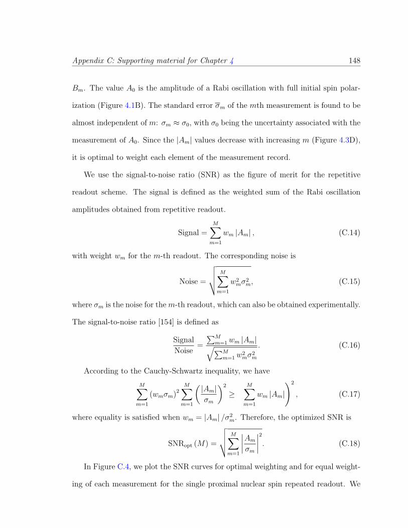
Appendix C: Supporting material for Chapter 4 148
Bm. The value A0 is the amplitude of a Rabi oscillation with full initial spin polar-
ization (Figure 4.1B). The standard error σm of the mth measurement is found to be
almost independent of m: σm ≈ σ0, with σ0 being the uncertainty associated with the
measurement of A0. Since the |Am| values decrease with increasing m (Figure 4.3D),
it is optimal to weight each element of the measurement record.
We use the signal-to-noise ratio (SNR) as the figure of merit for the repetitive
readout scheme. The signal is defined as the weighted sum of the Rabi oscillation
amplitudes obtained from repetitive readout.
Signal =M∑m=1
wm |Am| , (C.14)
with weight wm for the m-th readout. The corresponding noise is
Noise =
√√√√ M∑m=1
w2mσ
2m, (C.15)
where σm is the noise for the m-th readout, which can also be obtained experimentally.
The signal-to-noise ratio [154] is defined as
Signal
Noise=
∑Mm=1wm |Am|√∑M
m=1 w2mσ
2m
. (C.16)
According to the Cauchy-Schwartz inequality, we have
M∑m=1
(wmσm)2M∑m=1
( |Am|σm
)2
≥(
M∑m=1
wm |Am|)2
, (C.17)
where equality is satisfied when wm = |Am| /σ2m. Therefore, the optimized SNR is
SNRopt (M) =
√√√√ M∑m=1
∣∣∣∣Amσm∣∣∣∣2. (C.18)
In Figure C.4, we plot the SNR curves for optimal weighting and for equal weight-
ing of each measurement for the single proximal nuclear spin repeated readout. We

Appendix C: Supporting material for Chapter 4 149
0 10 20 30 40 50 601.0
1.2
1.4
1.6
1.8
2.0
2.2
M
SN
RHM
LSN
RH1
L
Figure C.4: Signal-to-Noise ratio for repetitive readout. The green data points corre-spond to the SNR where wm = 1 for all measurements of the Am amplitudes and σmuncertainties. The red data are for the optimized SNR values where wm = |Am|/σ2
m
and reach the best SNR improvement of 220%. The blue curves are the theoreticalfits to our model for measurement of the NV center electronic spin and fit well to thedata. Note that the model is identical for both cases.
see that for the equal weighting case, after M ≈ 20 the SNR begins to degrade. This
is because of the reduction of the signal amplitude Am for increasing m due to nuclear
spin depolarization, while the noise level σm remains almost constant. The weighting
factors wm allow for updating the measurement records to most efficiently use the
information with respect to the noise.

Appendix C: Supporting material for Chapter 4 150
C.5 Simulation for the Repetitive Readout
We have performed a numerical simulation for both repetitive readout schemes.
We use the transition matrix description to keep track of the state evolution. With
reasonable choice of imperfection parameters, we are able to obtainAm and SNRopt (M)
consistent with the experiment.
Transition matrices
We model 8 = 23 levels associated with the electronic spin and two nuclear spins
in the simulation. Because the quantum coherence does not change the outcome of
the repetitive readout, it is sufficient to track the probability distribution over these 8
levels. We use the array ~q = (q0↓↓, q0↓↑, q0↑↓, q0↑↑, q1↓↓, q1↓↑, q1↑↓, q1↑↑)T to represent the
probability distribution. We consider the transition matrices for various operations
characterized by imperfection parameters. For example, if initial state distribution is
~q0 and transition matrix is T , the final state distribution is T ~q0.
We now list the transition matrices for the operations that are used for spin
initialization and repetitive readout.
1) Transition matrix for MW1 π-pulse is
TMW1 = Wpi ⊗ I↓ ⊗ 12 +Wid ⊗ I↑ ⊗ 12, (C.19)
where
Wpi =
εMWres 1− εMW
res
1− εMWres εMW
res
Wid =
1− εMWdet εMW
det
εMWdet 1− εMW
det

Appendix C: Supporting material for Chapter 4 151
I↓ =
1 0
0 0
I↑ =
0 0
0 1
12 =
1 0
0 1
with εMW
res = 0.07 for the resonant transition and εMWdet = 0.01 for the ∆-detuned
transition (see Section C.1). Similarly the transition matrix for MW2 π-pulse is
TMW2 = Wpi ⊗ I↑ ⊗ 12 +Wid ⊗ I↓ ⊗ 12. (C.20)
2) The transition matrices for nuclear spin depolarization under optical illumina-
tion are
Tn1 = 12 ⊗
1− εn1
2εn1
2
εn1
21− εn1
2
⊗ 12 (C.21)
for n1, and
Tn2 = 12 ⊗ 12 ⊗
1− εn1
2εn1
2
εn1
21− εn1
2
(C.22)
for n2. The depolarization factors are εn1 = 0.05 for n1 after tgreen = 350 ns green
laser pulse, and εn2 = 0.42 and 0.63 for the second nuclear spin after 5 and 20 µs
green laser pulses (see Section C.3). During the M -step repetitive readout, the flip-
flop evolution between n1 and n2 during the short 1.5 µs interval between sequential
readouts may occur with probability about 5%, which is also effectively included into
εn2.
3) The transition matrix for optical pumping of the electronic spin is
TPump =
1− εpump,0 1− εpump,1εpump,0 εpump,1
⊗ 12 ⊗ 12, (C.23)
where εpump,0 and εpump,1 are the error probability for imperfect pumping. The char-
acteristic time for optical pumping of the electronic spin is τpump = 235 ns, so the 350

Appendix C: Supporting material for Chapter 4 152
ns green laser pulse has εpump,1 = 0.25. In addition, we also assume that there will
be εpump,0 = 2% of the population from m = 0 to m = 1 state.
4) The transition matrix for the RF π-pulse is
TRF =2 ⊗
1− εRF εRF
εRF 1− εRF
⊗ 12 (C.24)
where εRF < 1% based on our calibration, so we assume perfect RF π-pulse (i.e.,
εRF = 0) for simplicity. Similarly we also assume negligible error for the SWAP gate
on n1 and n2.
Simulation with transition matrices
Using the above transition matrices, we can obtain the evolution in probability
distribution for a given pulse sequence. For example, the distribution after k-step
repeated pumping of n1 is
~qk = (TPumpTRFTMW2)k ~q0, (C.25)
where ~q0 is the initial distribution. With these parameters, we first simulate and
obtain the amplitude of nuclear Rabi oscillation, with amplitude 0.61, consistent
with experimental observation of 0.60± 0.05.
For the pulse sequence provided in Figure 4.3B, the state for the first readout is
~q(δ)meas,1 = TRF (TMW1)δ ~qk=6, (C.26)
where δ = 0 for trivial MW1 pulse with duration t = 0, and δ = 1 for MW1 π-pulse
with duration t = π/ΩMW . The population difference in |0〉e between ~q(0)meas,1 and

Appendix C: Supporting material for Chapter 4 153
~q(1)meas,1 gives the normalized amplitude
|A1| =∣∣∣Prob
[~q
(0)meas,1
]− Prob
[~q
(1)meas,1
]∣∣∣ , (C.27)
where
Prob [~q] = q0↓↓ + q0↓↑ + q0↑↓ + q0↑↑ (C.28)
is the probability in the |0〉e state for distribution ~q.
The state for the following readout is
~q(δ)meas,m =
(TPumpTMW2) ~q(δ)meas,m−1 for even m
(TPumpTMW1) ~q(δ)meas,m−1 for odd m
, (C.29)
with m = 2, 3, · · · ,M . Finally, the normalized amplitude for the m-th readout is
|Am| =∣∣Prob
[~q(0)
meas,m
]− Prob[~q(1)
meas,m
]∣∣ . (C.30)
And
SNRopt (M) =
√√√√ M∑m=1
|Am|2. (C.31)
The simulation of Am and SNRopt (M) for the repetitive readout scheme assisted
with one qubits are shown in Figure 4.3DE. Similarly, we can also simulate Am and
SNRopt (M) measured for the repetitive readout scheme assisted with two qubits are
shown in Figure 4.4CD.

Appendix D
Supporting material for Chapter 5
D.1 Irradiation and annealing procedure
The sample used in the experiment described in Chapter 5 was an ultrapure
single crystal bulk diamond grown by chemical vapour deposition (CVD) provided
by Element Six Lta. (www.e6.com). The centers were created by irradiating 109
cm−2 nitrogen ions with energy of 6 keV, corresponding to an estimated average
implantation depth of 10 nm, as determined by simulations. The irradiating procedure
was done at CORE Lta. (California, USA). The sample was then annealed at 800 C
for 2 hours under a pressure no larger than 10−6 torr using a sputtering machine at
the Center for Nanoscale Science at Harvard University. This procedure leads to a
NV concentration of approximately 0.6 NV/µm2 corresponding to a yield of 4%. To
reliably distinguish shallow implanted ions from natural NV centers, a rare isotope
15N was used.
154

Appendix D: Supporting material for Chapter 5 155
D.2 Confocal and spin-RESOLFT microscopy
NV centers were probed using a custom-built confocal fluorescence microscope.
Two 532 nm laser beams provided optical excitation, one a Gaussian shaped beam and
the other a doughnut shaped beam. The two beams, which could be independently
switched using Acouto-Optic Modulators (AOMs - Crystal Technology and Isomet),
were combined on a polarised beam splitter before entering an oil immersion objective
(Nikon Plan Fluor 100x 1.3 NA). Fluorescence from the NV centers was collected back
through the objective, separated from the excitation path via a custom dichroic with
high surface flatness (Chroma Technology). The fluorescence was filtered (630− 750)
nm and focused onto a single-mode fibre connected to an avalanche photo detector
(APD - Perkin Elmer). Imaging was achieved by scanning the diamond sample under
the objective, using a digitized 3-axis piezo translation stage (Physical Instrument
P-733.3CD). The doughnut shaped mode was created by passing a Gaussian beam
through the center of a helical phase ramp (RPC Photonics), which adds a phase from
(0 to 2π) conditional on the azimuthal position. To prevent distortion of the doughnut
center due to beam focusing by the objective, the beam was circularly polarized by
placing a quarter-lambda waveplate immediately before the objective.
D.3 Generation of Doughnut beam
The doughnut shaped mode was created by passing a Gaussian beam through
the center of a helical phase ramp (RPC Photonics), which adds a phase from (0 to
2π) conditional on the azimuthal position. The exact expression for the doughnut
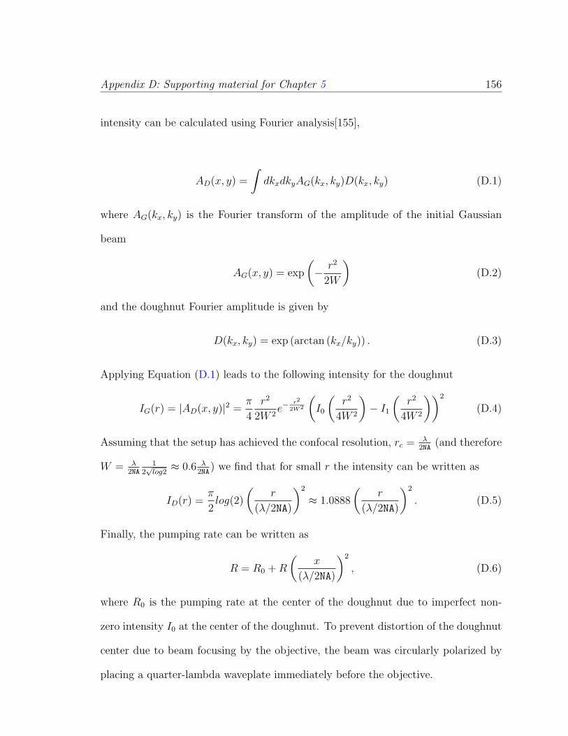
Appendix D: Supporting material for Chapter 5 156
intensity can be calculated using Fourier analysis[155],
AD(x, y) =
∫dkxdkyAG(kx, ky)D(kx, ky) (D.1)
where AG(kx, ky) is the Fourier transform of the amplitude of the initial Gaussian
beam
AG(x, y) = exp
(− r2
2W
)(D.2)
and the doughnut Fourier amplitude is given by
D(kx, ky) = exp (arctan (kx/ky)) . (D.3)
Applying Equation (D.1) leads to the following intensity for the doughnut
IG(r) = |AD(x, y)|2 =π
4
r2
2W 2e−
r2
2W2
(I0
(r2
4W 2
)− I1
(r2
4W 2
))2
(D.4)
Assuming that the setup has achieved the confocal resolution, rc = λ2NA
(and therefore
W = λ2NA
12√log2≈ 0.6 λ
2NA) we find that for small r the intensity can be written as
ID(r) =π
2log(2)
(r
(λ/2NA)
)2
≈ 1.0888
(r
(λ/2NA)
)2
. (D.5)
Finally, the pumping rate can be written as
R = R0 +R
(x
(λ/2NA)
)2
, (D.6)
where R0 is the pumping rate at the center of the doughnut due to imperfect non-
zero intensity I0 at the center of the doughnut. To prevent distortion of the doughnut
center due to beam focusing by the objective, the beam was circularly polarized by
placing a quarter-lambda waveplate immediately before the objective.

Appendix D: Supporting material for Chapter 5 157
D.4 Spin imaging resolution
The spin-RESOLFT signal is proportional to f(x) = n0(x)IG(x), where n0 is the
population of the ms = 0 state, IG = exp(−α(x/rC)2) is the intensity profile of the
gaussian beam used for readout of the electronic spin, rC = λ/2NA is the confocal
resolution and α = 4/log(2). n0 depends on the duration of the doughnut beam tD;
it can be evaluated by solving the rate equations of the system given in Figure D.3.
In the limit of large lifetime of the spin transition, it is given by n0 = exp(−RxtD),
where Rx = εkx is the position-dependent optical depletion rate out of the ms = 1
state (i.e., polarization rate to the ms = 0 state measured after waiting for the non-
radiative relaxation from the singlet state to the ms = 0 state), kx is the intensity
profile of the doughnut-shaped beam and ε is the branching ratio of the spin changing
(ms = 1 → ms = 0) decay relative to the total decay of the excited state. In the
unsaturated regime, Rx = R0 + αΓ(x/rC)2, where Γ = κε is proportional to the
optical excitation rate associated with the maximal intensity of the doughnut κ, and
R0 = εκ0 is proportional to the intensity of the doughnut center and the corresponding
excitation κ0. The resolution r is defined by f(x) = exp(−α(x/∆r)2). Solving for ∆r
leads to Eq. (1) in Chapter 5. In the case of a perfect doughnut beam the ultimate
resolution is determined by the maximum values of Γ = γε and TD ∼ T1. Thus
leading to an improvement in resolution relative to the diffraction limit of a confocal
microscope of√εγT1.
In our experiments, the resolution is limited by a small imperfection of the doughnut-
zero intensity. We can find the maximum achievable resolution by using a model that
includes a back pumping process which brings the electronic spin from the ms = 0

Appendix D: Supporting material for Chapter 5 158
to the ms = 1 state, and finite spin lifetime. Consider the rate equations of our two
level system (ms = 0 and ms = 1),
dn0
dt= Rxn1 − γ0→1(n1 − n0) (D.7)
and n1 = 1− n0. The solution for this equation is,
n1 =γ1 +Rx
2γ0→1 +Rx
(1− e−(2γ0→1+Rx)tD) (D.8)
The resolution δr is defined by the FWHM condition n2(Rr/2, t) = 12n2(R0, t). The
maximum improvement in resolution relative to the diffraction limit of a confocal
microscope is given by
∆r/rC =√R0/Γ
√1 + 2γ0→1/R0 (D.9)
for an optimal doughnut duration tD = log[(3γ0→1 +2R0)/(γ0→1 +R0)]/(2γ0→1 +R0),
where γ0→1 is the total rate out of the electronic spin ms = 0. In the limit of
long spin lifetime (γ0→1 R0), the maximum improvement in resolution is given by√R0/Γ =
√κ0/κ, i.e., the intensity of the doughnut center relative to the maximum
doughnut intensity. In our experiments, κ0/κ ≈ 1%, which is in a good agreement
with our 10-fold improvement in resolution relative to the diffraction limit.
To demonstrate the nanoscale resolving power of our spin sensitive far-field optical
technique, we imaged NV centers in bulk diamond separated by less than the diffrac-
tion limit. Figure D.3a shows a pair of individual NV centers that cannot be resolved
using confocal microscopy. However, an optically detected ESR measurement per-
formed in this location displays multiple spectral lines (Figure D.3b), indicating the
presence of multiple NV centers with different crystallographic orientations relative to
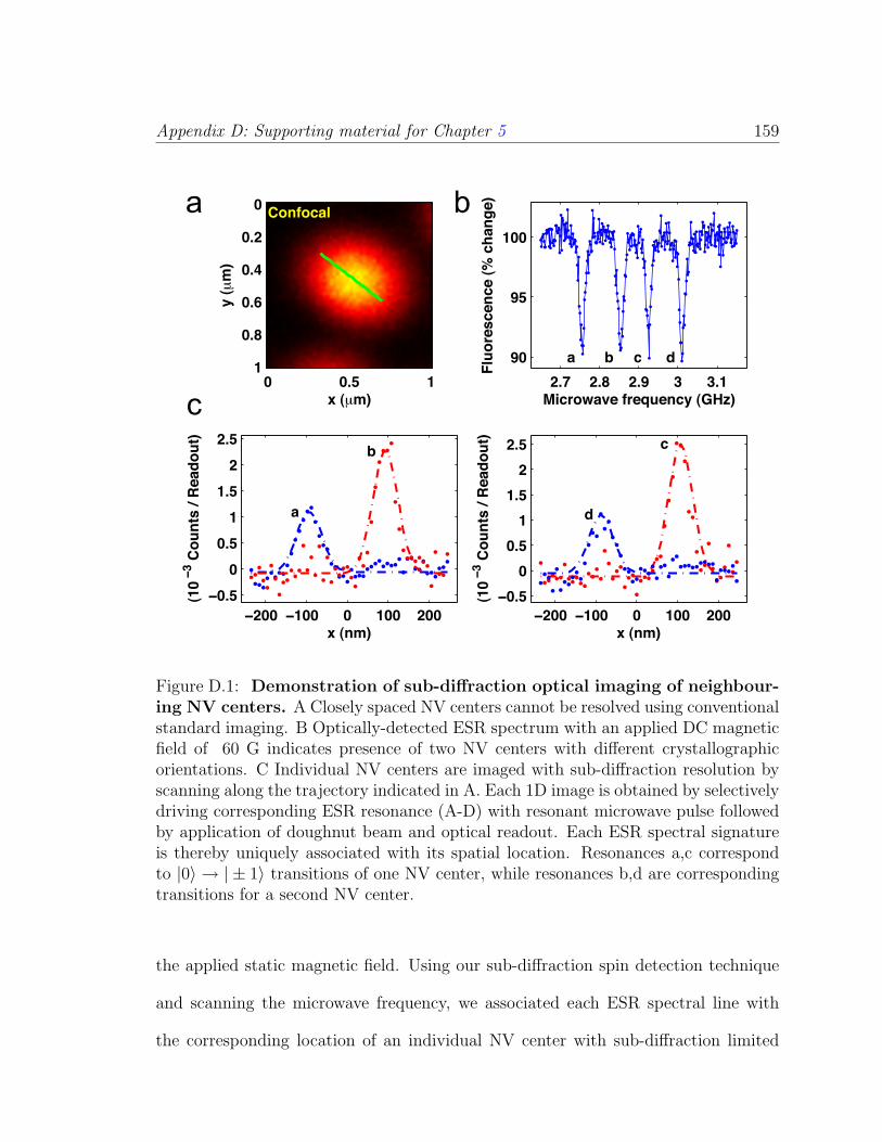
Appendix D: Supporting material for Chapter 5 159
!!"" !#"" " #"" !""
!"$%
"
"$%
#
#$%
!
!$%
&'()*+
(#"'!,'-./)01'2'3456./0+
5
7
!!"" !#"" " #"" !""
!"$%
"
"$%
#
#$%
!
!$%
&'()*+
(#"'!,'-./)01'2'3456./0+ 8
6
!$9 !$: !$; , ,$#
;"
;%
#""
<=8>.?5@4'A>4B/4)8C'(DEF+
GH/.>4184)84'(I'8J5)K4+
5 7 8 6
&'(µ*+
C'(µ*+
-.)A.85H
" "$% #
"
"$!
"$L
"$M
"$:
#
a b
c
Figure D.1: Demonstration of sub-diffraction optical imaging of neighbour-ing NV centers. A Closely spaced NV centers cannot be resolved using conventionalstandard imaging. B Optically-detected ESR spectrum with an applied DC magneticfield of 60 G indicates presence of two NV centers with different crystallographicorientations. C Individual NV centers are imaged with sub-diffraction resolution byscanning along the trajectory indicated in A. Each 1D image is obtained by selectivelydriving corresponding ESR resonance (A-D) with resonant microwave pulse followedby application of doughnut beam and optical readout. Each ESR spectral signatureis thereby uniquely associated with its spatial location. Resonances a,c correspondto |0〉 → | ± 1〉 transitions of one NV center, while resonances b,d are correspondingtransitions for a second NV center.
the applied static magnetic field. Using our sub-diffraction spin detection technique
and scanning the microwave frequency, we associated each ESR spectral line with
the corresponding location of an individual NV center with sub-diffraction limited

Appendix D: Supporting material for Chapter 5 160
resolution (Figure D.3c). In particular, sub-diffraction spin imaging scans along the
trajectory indicated in Figure D.3a, taken for each ESR transition frequency, reveal
that two NV centers are responsible for the observed ESR spectrum: each NV cen-
ter has two spectral ESR lines corresponding to the |0〉 → | + 1〉 and |0〉 → | − 1〉
transitions.
D.5 Measurements of local magnetic field environ-
ment with sub-diffraction resolution
As described in Chapter 5, individual NV centers can be resolved, independently
manipulated and read-out using our technique. Here we individually measure the
response of two NV centers to their local magnetic environment using Rabi and spin-
echo techniques. By placing the center of the doughnut over one NV center, the other
NV center is polarized and only contributes a constant background to the fluorescence
signal. Figure D.2 shows the raw data for Rabi measurements of the two NV centers
in Figure 5.3 when the doughnut zero is placed over Center 1 (upper-left panel) and
Center 2 (bottom-left panel). When the two curves are added together (green line,
right panel), the confocal measurement (taken at the position of Center 1) is recovered
(dotted line in Figure D.2).
The observed modulations of the Rabi oscillations shown in Figure 5.3c (and
Figure D.2) reveal the different magnetic fields experienced by each NV center. These
modulations are caused by hyperfine induced splitting in the NV center’s electronic
transition (ms = 0→ 1) associated with the 15N nuclear spin (I = 12). A simple model

Appendix D: Supporting material for Chapter 5 161
0 200 400 600 800 1000
0.9
0.95
1
Microwave pulse width (ns)
Fluo
resc
ence
(% ch
ange
)Center 1
0 200 400 600 800 10000.85
0.9
0.95
1
Microwave pulse width (ns)
Fluo
resc
ence
(% ch
ange
)
Center 2
0 200 400 600 800 10000.7
0.75
0.8
0.85
0.9
0.95
1
Microwave pulse width (ns)
Fluo
resc
ence
(% ch
ange
)
Center 1 + Center 2
Figure D.2: Realization of spin-RESOLFT Rabi measurements. Rabi oscilla-tions for each NV center were measured by centering the doughnut on one of the NVcenters. The addition of the two Rabi oscillation data curves (green line, right panel)corresponds to the confocal measurement of both NV centers as expected (pink dots,right panel).
for the probability of finding the electronic spin in the ms = 0 state, P0, assumes that
on average the 15N nuclear spin is half of the time in its spin down state and the other
half of the time in its spin up state. Thus, P0 is just the average of the dynamics of
two two-level systems with different splittings. For a two-level system with states |0〉
and |1〉, Rabi frequency Ω and detuning δ, the probability to find the system in state
|1〉 (starting from state |0〉) is given by ( ΩΩe
)2 sin2 Ωeτ , where Ω2e = Ω2 +δ2. Therefore,
P0 in our case is given by
P0 =1
2
(2−
(Ω
Ω1
)2
sin2(Ω1τ/2)−(
Ω
Ω2
)2
sin2(Ω2τ/2)
)(D.10)
where Ω21 = Ω2 +δ2
1 and Ω22 = Ω2 +δ2
2. If Ω δ, the modulation frequency is given by

Appendix D: Supporting material for Chapter 5 162
∆Ω = Ω2−Ω1 ≈ (δ1 + δ2)(δ1− δ2)/2Ω. Since δ1 + δ2 = 2(f0− f) and δ2− δ1 = A, the
modulation frequency for an NV center is given by ∆Ω = (ν0−ν)A/Ω, where ν0 is the
frequency of the electronic transition ms = 0→ 1, ν is the microwave frequency and
A = 3.05 MHz[87] is the hyperfine splitting induced by the 15N nuclear spin present
on each of our NV centers (see section Samples).
Modulations appear when the microwave frequency is detuned from the central
transition νi0 = ∆ + γeBi, where Bi is the local magnetic field along the NV axis of
center i, ∆ is the zero-field splitting, and γe is the gyromagnetic ratio of the electronic
spin. In other words, modulations appear when the two hyperfine transitions are
driven with different detunings. The difference in the modulation frequencies of each
NV center (∆Ω2 − ∆Ω1 = 1.3 − 0.5 = 0.8 MHz) reveals a difference in the static
magnetic field experienced by each NV center of about ∆B = 1 G.
Spin echo measurements can reveal even more subtle differences in the local en-
vironment between the two NV centers. In our measurements (Figure 5.3d), the
dominant contribution comes from interactions between the electronic spin of the NV
center and the 15N nuclear spin and 13C nuclear spin bath. The spin echo signal can
be written as [53] p(τ) = 1+S(τ)2
, where S(τ) is the pseudo spin which can be written
as the multiplication of all individual nuclear spin contributions. The first collapse
and first revival of the NV spin echo signal can thus be approximated by
S(τ) = S15N(τ)(e−(τ/τC)4
+ ce−((τ−τR)/τC)4), (D.11)
where we have phenomenologically grouped the effect of all 13C nuclear spins in the
exponential decays, and where τC is the collapse rate[53] given by τC = 13µs√
5GB
, B
is the local magnetic field, τR is the revival time, c is the contrast of the first revival.

Appendix D: Supporting material for Chapter 5 163
The pseudo spin for the 15N nuclear spin is given by
S15N(τ) = 1− |Ω15N,0 × Ω15N,1|2|Ω15N,0|2|Ω15N,1|2 sin(Ω15N,0τ/2)2 sin(Ω15N,1τ/2)2, (D.12)
where Ω15N,ms is the Larmor frequency of 15N when the electron is in state ms. The
blue lines in Figure 5.3d are fitted to Equation (D.11). While Center 2 shows good
coherence (c = 0.86), Center 1 shows no revival of the signal (c = 0). The absence
of revival for Center 1 can be due to an unfavorable distribution of nearby pairs of
13C nuclear spins that quickly decohere the electronic spin [23], or due to nearby
paramagnetic impurities or other defects. The position of the first revival for Center
2, τR = 13.5 µs, is set by the Larmor precession of 13C, τ−1R = ωC13 = γC13B,
corresponding to a local magnetic field of B = 69 G. The high frequency oscillations
(Ω15N,1) correspond to the hyperfine interaction between the electronic spin and the
15N nuclear spin, Ω15N,1 ≈ A = 3.05 MHz. Meanwhile the slow frequency component
of the dynamics, Ω15N,0 = 360 kHz, corresponds to the Larmor frequency of the 15N
nuclear spin when the electron is in state ms = 0. We immediately notice that the
slow frequency component is too large to be explained by the bare Larmor frequency
of 15N at 69 G, γN15B = 30 kHz. This slow frequency component Ω15N,0 is enhanced
by virtual transitions between the NV electronic spin and the 15N nuclear spin. This
enhancement is of the form (see Appendix A.4),
∆g = −(3|ms| − 2)gnγe∆γn
Axx Axy Axz
Ayx Ayy Ayz
0 0 0
. (D.13)
In the case of 15N , the hyperfine interaction is isotropic[87] and the enhancement is
given by ∆g0 ≈ 7.8 (corresponding to a gyromagnetic increment factor of 2(γ2/γn)A/∆ ≈

Appendix D: Supporting material for Chapter 5 164
14). Therefore, Ω15N,0 ≈ 14γnB⊥ corresponding to a perpendicular field to the NV
axis of B⊥ = 60 G. This value is in agreement with the component of the magnetic
field parallel to the NV axis that leads to the observed splitting in the ESR spectrum
(Figure 5.3a), B|| = 36 G (B =√
362 + 592 ≈ 69 G).
D.6 Inhibition of Electron-Spin Rabi Oscillations
via Quantum Zeno-like Effect
In Chapter 5 (Figure 5.4a), we demonstrate that a green laser beam can inhibit
coherent electron-spin transitions of a single, isolated NV center driven by a resonant
microwave pulse. In Figure 5.4b we exploit this property to perform spatially-selective
coherent electron-spin Rabi oscillations on one of two closely spaced, 150 nm, NV
centers, using a doughnut shaped laser beam.
In Figure 5.4a we investigate this suppression mechanism by applying the pulse
sequences S1 and S2. Our analysis requires knowledge of the populations (ρ0,0, ρ1,1
, ρ1A1,1A1) of the ms = 0, ms = ±1 and 1A1 manifolds right after state preparation.
To determine these quantities we record the fluorescence,
f(τd) = c0,0ρ0,0(τd) + c1,1ρ1,1(τd) + c1A1,1A1ρ1A1,1A1(τd), (D.14)
of a single NV center for two different times τd T1A1 and τd T1A1 , where τd is
the time defined in S1 and S2 of Figure 5.4a, T1A1 = 300 ns is the lifetime of the
singlet, and ci,i are the fluorescence rates for the corresponding states, which can be
determined experimentally. Since the singlet 1A1 nearly always decays non-radiatively
into the ms = 0 state (and hence c1A1,1A1 = 0)[111] we can extract the populations

Appendix D: Supporting material for Chapter 5 165
ρi,i, which are shown in Figure 5.4a, from measuring the fluorescence at τd T1A1
and τd T1A1 and using the relation ρ0,0 + ρ1,1 + ρ1A1,1A1 = 1. This allows us to find
the system of equations
1 = ρ0,0 + ρ1A1,1A1 + ρ1,1
f(τd 50ns) = c0,0ρ0,0 + c1,1ρ1,1
f(τd 50ns) = c0,0(ρ0,0 + ρ1A1,1A1) + c1,1ρ1,1, (D.15)
which defines the population ρi,i for τd T1A1.
Figure 5.4b demonstrates that a green doughnut-shaped laser beam inhibits electron-
spin Rabi oscillations on one of two closely spaced NV centers (Center 2, sitting out-
side the central doughnut null), while allowing Rabi oscillations to proceed on Center
1, which sits in the zero of the doughnut. The two NV centers have a spatial separa-
tion of about 150 nm. To verify that Center 1 can undergo coherent Rabi oscillations
while Center 2 is kept in the ms = 0 state, two experiments (pulse sequences S3 and S4
in Figure 5.4b) were performed and subtracted from each other. If Center 2 remains
in the ms = 0 state, a constant signal is expected for the difference. In this subtrac-
tion procedure we accounted for contrast reduction in the spin-RESOLFT readout of
Center 1 by multiplying the results of experiment S4 by 1.3. (This weighting factor is
determined from a separate experiment, in which both centers were prepared in the
state ms = 1 and imaged with spin-RESOLFT). The signals were normalized relative
to the ideal (unperturbed) Rabi oscillation signal for Center 1.
In this section, we describe in detail the optical inhibition of electron spin Rabi
oscillations using a doughnut beam (Figure 5.4b in Chapter 5). The basic idea can
be explained by considering a simple two-level system (with states |0〉 and |1〉), which

Appendix D: Supporting material for Chapter 5 166
undergoes Rabi oscillations (with Rabi frequency Ω) and which is subject to an effec-
tive dephasing (with dephasing rate γp). The system dynamics is then governed by
the Hamiltonian H = −Ω2σx (where ~σ are Pauli matrices) combined with the decay
of the off-diagonal matrix elements of the density matrix ρ with rate γp. Formally,
this is described by the following master equation:
dρ
dt= i
[Ω
2σx, ρ
]− γp
4[σz, [σz, ρ]] . (D.16)
Suppose the system starts in the |0〉 state, i.e., P0 (t = 0) = 1. We analytically
solve the master equation and obtain the probability of being in the |0〉 state as a
function of time:
P0 (t) =1
2
(1 +
Γ+e−Γ−t − Γ−e
−Γ+t
Γ+ − Γ−
), (D.17)
where Γ± = 12
(γp ±
√γ2p − 4Ω2
). We may also use the approximate form:
P0 (t) ≈
12
(1 + cos (Ωt) e−γpt/2
)for Ω γp
12
(1 + exp
(−Ω2
γpt))
for Ω γp
. (D.18)
For Ω γp, the two-level system undergoes Rabi oscillations with an amplitude
decay rate γp/2. This scenario approximately describes the evolution of Center 1
[blue curve in Figure 5.4b in Chapter 5]: there the amplitude decay comes from
a combination of T ∗2 decay and of the dephasing due to the imperfect zero of the
dougnut. On the other hand, for Ω γp, the oscillation dynamics is inhibited, and
the system remains in the initial state |0〉 with a slow spin-relaxation rate Ω2/γp,
which is inversely proportional to γp. This scenario, which we refer to as a quantum
Zeno-like effect [48], approximately describes the evolution of Center 2 [green curve
in Figure 5.4b in Chapter 5]. In particular, the scheme succeeds if the spin-relaxation

Appendix D: Supporting material for Chapter 5 167
0.00 0.05 0.10 0.15 0.20 0.250.0
0.2
0.4
0.6
0.8
1.0
t Μs
P0
(b)(a)
Figure D.3: title. (a) 5-level system used to model inhibition of electron-spin Rabioscillations. γ ≈ 1/(13 ns) = (2π)12.2 MHz, γS ≈ 1/(300 ns), and Ω = (2π)2 MHz.(b) Calculated inhibition of electron-spin Rabi oscillations: the blue curve has κ = 0and shows an uninhibited Rabi π-pulse [analogous to Center 1 evolution shown as theblue curve in Figure 5.4b of Chapter 5]; the green (red) curve has κ = γ and ε = 0.3(ε = 0) and demonstrates the inhibition of the Rabi oscillations. The green curve isanalogous to Center 2 evolution shown as the green curve in Figure 5.4b of Chapter5. The fact that the red curve stays close to 1 confirms that the quantum Zeno-likeeffect due to dephasing (and not the optical pumping from |g1〉 to |g0〉) plays thedominant role in suppressing Rabi oscillations of Center 2. The value (here ≈ 0.9) ofthe red curve at the final time π/Ω can be used as a rough estimate of preservationof nuclear spin coherence on Center 2 in future experiments.
rate in Center 2 over the course of a π-pulse on Center 1 is much less than unity:
1−P0(t) ≈ (1/2)(Ω2/γp)∗(π/Ω) = πΩ/(2γp) 1. In other words, for times t γp/Ω2
the center is ”frozen” in the ground state.
In reality, the experimental situation is more complicated than this simple two-
level model. Specifically, we must account for processes in which the spin is first
flipped to state |1〉 and subsequently repolarized to state |0〉. We therefore model
the experiment by considering the five-level system shown in Figure D.3(a). The five
states are the ground states |g0〉 with ms = 0 and |g1〉 with ms = 1, the excited states
|e0〉 with ms = 0 and |e1〉 with ms = 1, as well as the singlet |S〉. In addition to

Appendix D: Supporting material for Chapter 5 168
the coherent evolution with Rabi frequency Ω, the system is subject to incoherent
excitation (caused by the green laser) from the ground to the excited states with rate
κ. Moreover, the excited states decay down to the triplet with rate γ ≈ 1/(13 ns) =
(2π)12.2 MHz [111]. At the same time, the state |e1〉 decays down to the singlet
with rate εγ, where we take ε = 0.3, while the singlet decays to |g0〉 with rate γS ≈
1/(300 ns). After extracting Ω = (2π)2 MHz from the uninhibited Rabi oscillations
of Center 1 [Figure 5.4b in Chapter 5] and κ ≈ γ (on Center 2) from the fluorescence
saturation curve (not shown), we know all the parameters and can compute the
resulting evolution of Center 2 over time π/Ω, which is sufficient for a π pulse on the
uninhibited Center 1. We begin with Center 2 in the state |g0〉, keep the microwave
and the green light on for time t, then allow the population to relax to |g0〉 and |g1〉,
and plot in green in Figure D.3(b) the resulting population P0 of |g0〉 for Center 2 as
a function of t. In agreement with the green curve in Figure 5.4b of Chapter 5, we
see that the population stays within a few percent of the initial population of unity,
while Center 1 (with κ ≈ 0) does a Rabi π pulse (blue curve). The reason why the
blue curve in Figure 5.4b of Chapter 5 does not show a perfect π-pulse is because the
doughnut zero is imperfect and because T ∗2 is finite.
To confirm that the observed inhibition indeed comes from Zeno-like effects and
not from re-pumping of the electron spin from |g1〉 to |g0〉 via the singlet, we plot in
red in Figure D.3(b) the equivalent of the green curve except with ε = 0, i.e. we turn
off the |g1〉 → |g0〉 pumping process. We observe that the population still stays mostly
in |g0〉, confirming that it is indeed Zeno-like dynamics that is largely responsible for
the inhibition. In fact, for our parameters (κ Ω), the red curve has a simple

Appendix D: Supporting material for Chapter 5 169
analytical form
P0(t) =1
2
(1 + e−
γκ+γ
Ω2
κt
). (D.19)
Since both |g0〉 and |g1〉 are excited with rate κ, the coherence between these two levels
decays with rate κ, so κ plays the role of the dephasing rate γp from our two-level
model above. The prefactor γ/(κ + γ) in front of Ω2/κ is the population that is in
the ground state triplet, while the remainder is in the excited state and is unaffected
by Ω since the corresponding transition in the excited state is highly off-resonant
(and was, thus, not included in the model). Under this approximation, the transition
probability for Center 2 over time π/Ω is 1−P0(t) ≈ [γ/(κ+ γ)][πΩ/(2κ)], which for
our parameters is ≈ 0.1, which is much smaller than unity, as desired. This value can
be further reduced by going to larger green laser powers or smaller Rabi frequencies.
One eventual goal of this demonstrated inhibition is to allow quantum information
stored in a nuclear spin degree of freedom (coming from the nitrogen or a nearby
carbon-13) to be controllably manipulated in each NV center. Provided that the
electron state of the illuminated NV center (Center 2) is kept in |ms = 0〉, the
state of the corresponding nuclear spin would be preserved [74], while the nuclear
spin associated with Center 1 can be prepared, coherently manipulated, or detected
with subwavelength resolution. The performance of this technique can be directly
evaluated from our measurements. Specifically, the error induced on the nuclear spin
associated with illuminated Center 2 is proportional to 1−P0 ≈ 0.1 1. This small
error indicates that the state of the nuclear spin associated with Center 2 can be well
preserved while we manipulate Center 1.

Appendix E
Supporting material for Chapter 6
E.1 Dangling bond representation and character
table
In this appendix we show in detail how to find the electronic representation for the
case of the NV center. The NV center contains a vacancy that results in broken bonds
in the system. In the tight binding picture, this means that three C atoms and one N-
atom do not have enough immediate neighbor atoms to form a covalent bond for each
of their valence electrons. These unpaired electrons are called ’dangling bonds’. In
the case of the NV center, we consider a simple model consisting of four sp3 dangling
bonds, where three of them are centered on each of the three carbon atoms around
the vacancy and the fourth dangling bond is associated with the nitrogen atom. The
point group symmetry is C3v and its elements are the identity, rotations around the
z (NV-axis) by ±2π/3 and three vertical reflection planes where each contains one of
170

Appendix E: Supporting material for Chapter 6 171
the carbons and the nitrogen.
As discussed in Section 6.2, it is possible to construct the representation of the
dangling bonds for the point group they belong to. Consider Figure E.1 where the
z axis is pointing out of the paper. The dangling bonds σ1, σ2, σ3, σN transform
into one another under the operations of the C3v group. In this representation, each
operation can be written as a 4x4 matrix, as shown in Figure E.1. As representations
depend on the particular choice of basis, it is customary to use the sum of the diagonal
of each matrix (characters). Note that the character for matrices belonging to the
same class is the same, so in short the character representation for the dangling bonds
is Γσ = 411. This representation is clearly reducible, as it can be decomposed by
the irreducible representation of the C3v group given in Table E.1[156].
Table E.1: Character and bases table for the double C3v group. Examplesof functions that transform under a particular representation are z, x2 + y2, z2which transform as the IR A1, Rz transforming as A2 and the pair of functions(x, y), (Rx, Ry), (xy, x
2 − y2), (yz, xz) for the E IR.
C3v E C3 3σv E 2C3 3σvA1 1 1 1 1 1 1A2 1 1 -1 1 1 1E 2 -1 0 2 -1 0E1/2 2 1 0 -2 -1 0
1E3/2 1 -1 i -1 1 −i2E3/2 1 -1 −i -1 1 i
Application of Equation (6.1) gives the following combination of σ’s: aC =
(σ1 + σ2 + σ3) /3, ex = (2σ1 − σ2 − σ3) /√
6, ey = (σ2 − σ3)√
2, aN = σN, where
aC and aN transform as the totally symmetric irreducible representation A1, and ex
and ey transform as functions of the IR E. Note that the e states transform as vectors

Appendix E: Supporting material for Chapter 6 172
E C−3C+3
σd σe σf
Γσ :
11
11
,
1
11
1
,
1
11
1
,
1
11
1
,
1
11
1
,
1
11
1
.Γσ :
σ1
σ2
σ3
σN
σdσe
σf
Figure E.1: Schematic of the NV defect and dangling bond representation.(Top) Schematic of the dangling bond orbitals used to represent the NV defect. Thesymmetry axis or NV axis is pointing out of the plane of the page. The dashed linesrepresent the three vertical reflections planes of the C3v group. (Bottom) Matrixrepresentation of the dangling bonds.
in the plane perpendicular to the NV axis.
Next, we model the electron-ion interaction to find out the ordering of these states.
This interaction can be written in the basis of the dangling bonds σi as,
V = vn|σN〉〈σN |+∑i
vi|σi〉〈σi|+ hn|σi〉〈σN |+∑i>j
|σi〉〈σj|hc (E.1)
where vi < 0 is the Coulomb interaction of orbital σi at site i and hc is the ex-
pectation value of the interaction between orbitals σi and σi+1 at site i = 1, 2, 3.
This interaction, which transforms as the totally IR A1, not only sets the order of

Appendix E: Supporting material for Chapter 6 173
the orbitals but also mixes orbitals aN and aC . This is as expected since both wave
functions transform as the totally symmetric representation A1 as well as the interac-
tion between them so that the representation for the matrix element also transform as
Γ〈〉 = Γa⊗ΓσN⊗Γint = A1 ⊃ A1. The following concept is of major importance: when-
ever a matrix element contains the totally symmetric representation, its expectation
value might be different from zero[130]. This interaction leads to the new basis[18]
a1(1) = αac+βan, a1(2) = αan+βac, ex = (2σ1 − σ2 − σ3) /√
6, ey = (σ2 − σ3)√
2,
with energies Ea1(1),a1(2) = 12(vc + 2hc + vn) ± 1
2∆, vc − hc, vc − hc, respectively,
where ∆ =√
(vc + 2hc − vn)2 + 12h2n, α2 = 1 − β2 = 3h2
n/∆Ea1(1). We see that
the most symmetric state is lowest in energy, which is usually the case for attractive
interactions.
E.2 Ordering of singlet states
Here we show that two states belonging to the same irreducible representation
should have the same expectation value for their Coulomb interaction. We first note
that the expectation value of an operator is a classical number and it should not
depend on the particular coordinate system in use. In particular, this expectation
value should be invariant under any operation of the C3v group of the NV center.
The Coulomb interaction is totally symmetric and therefore not affected by any ro-
tation, and the wavefunctions ex, ey transform as the irreducible representation E.
Therefore, we can get more information about these expectation values by projecting

Appendix E: Supporting material for Chapter 6 174
them on the totally symmetric irreducible representation A1,
(ab, V, cd) =1
h
h∑R=1
χe (PR(a)PR(b), V, PR(c)PR(d)) . (E.2)
We find as expected that
(1E1, V,1E1) =
1
2(1E1, V,
1E1) +1
2(1E2, V,
1E2), (E.3)
which means that the states (1E1, V,1E1) and (1E2, V,
1E2) have the same energy, as
required by symmetry.
E.3 Spin-spin interaction
In order to analyze the effect of spin-spin interactions (Equation 6.6) from the
perspective of group theory, we first rewrite this interaction to identify spatial and
spin terms that transform as IR objects in the point group,
hss = −µ0g2β2
4π
[1− 3z2
4r3(s1+s2− + s1−s2+ − 4s1zs2z)
+3
4
x2 − y2
r3(s1−s2− + s1+s2+)
+i3
2
xy
r3(s1−s2− − s1+s2+)
+3
2
xz
r3(s1−s2z + s1zs2− + s1+s2z + s1zs2+)
+i3
2
yz
r3(s1−s2z + s1zs2− − s1+s2z − s1zs2+)
],
where x, y and z are directional cosines and s± = sx± isy. In the case of C3v, for the
unperturbed center, the expectation values of the 4th and 5th terms are not zero in
the spatial manifold of the excited state |X〉, |Y 〉 because the center lacks inversion
symmetry and therefore we cannot neglect them. However, these terms might be

Appendix E: Supporting material for Chapter 6 175
neglected when considering other defects with inversion symmetry. We note now that
the spatial part of the first term transforms as the totally symmetric representation
A1, while the 2nd and 3rd terms transform as the irreducible representation E. The
reader can check which IR these combinations belong to by looking at the character
table in the appendix. Therefore, their expectation values can be written as
µ0
4πg2β2
⟨1− 3z2
4r3
⟩= ∆(|X〉〈X|+ |Y 〉〈Y |)
µ0
4πg2β2
⟨3x2 − 3y2
4r3
⟩= ∆′(|X〉〈X| − |Y 〉〈Y |) (E.4)
µ0
4πg2β2
⟨3xy + 3yx
4r3
⟩= ∆′(|X〉〈Y |+ |Y 〉〈X|),
µ0
4πg2β2
⟨3xz + 3zx
4r3
⟩= ∆′′(|Y 〉〈Y | − |X〉〈X|),
µ0
4πg2β2
⟨3zy + 3yz
4r3
⟩= ∆′′(|X〉〈Y |+ |Y 〉〈X|),
where |X〉 and |Y 〉 are the two electron states given in Table 6.1. Note that, for
symmetry reasons, the second and third relations are characterized by the same pa-
rameter ∆′, while the last two relations are characterized by the same parameter ∆′′.
Similarly, it is possible to write the spin operators in the spin basis of the two holes,
|αα〉, |αβ〉, |βα〉, |ββ〉, e.g., s1+s2− = |αβ〉〈βα|. Using these relations and Equation
(E.4), the hamiltonian in the fundamental bases of the excited state of the NV center

Appendix E: Supporting material for Chapter 6 176
is
Hss = −∆(|X〉〈X|+ |Y 〉〈Y |) (E.5)
⊗ (|αα〉〈αα|+ |ββ〉〈ββ| − 2|αβ + βα〉〈αβ + βα|)
−∆′(|X〉〈X| − |Y 〉〈Y |)⊗ (|αα〉〈ββ|+ |ββ〉〈αα|)
−i∆′(|X〉〈Y |+ |Y 〉〈X|)⊗ (|ββ〉〈αα| − |αα〉〈ββ|)
+∆′′ (|Y 〉〈Y | − |X〉〈X|)
⊗ (|αβ + βα〉〈αα− ββ|+ |αα− ββ〉〈αβ + βα|)
+i∆′′ (|Y 〉〈Y | − |X〉〈X|)
⊗ (|αβ + βα〉〈αα + ββ| − |αα + ββ〉〈αβ + βα|) . (E.6)
Finally, to see the effect of this interaction on the excited state triplet more clearly,
we can write Hss in terms of the eigenstates of the unperturbed defect (see Table 6.1).
This leads to Equation (6.7).
E.4 Strain and electric field
The effect of strain on the electronic structure of the defect can be obtained from
the effect of the electron-nuclei Coulomb interaction on the eigenstates of the defect.
In our example, the Coulomb interaction is given by Equation (E.1). However, when
the positions of the atoms are such that the symmetry of the defect is reduced,
we should allow for different expectation values of the matrix elements, i.e., hij =
〈σi|V |σj〉 and hin = 〈σi|V |σN〉. We have assumed that the self interactions, vc and
vn, do not change as the electrons follow the position of the ion (Born Oppenheimer

Appendix E: Supporting material for Chapter 6 177
approximation). To relate the matrix elements to the ionic displacements, we can
assume as a first approximation that the electron orbitals are spherical functions,
and therefore the matrix elements can be parametrized by the distance between ions,
hij (qi, qj) = hij (|qi − qj|), so that we can write
hij (|qij|) ≈ hij(|q0
ij|)
+1
|qij|∂hij∂qij
(qi − qj)∣∣∣∣0
· (δqi − δqj) + .... (E.7)
The change in the matrix elements is linear in the atomic displacements. In turn, the
atomic displacements are related to the strain tensor by δqi = eqi, and therefore the
change in the matrix element is given by
δhij (|qij|) ≈ 1
|qij|∂hij∂qij
(qi − qj)T e (qi − qj)∣∣∣∣0
. (E.8)
Under these considerations, it is straightforward to calculate the effect of strain on
the eigenstates of the defect. For simplicity, we write here only the effect of strain on
the degenerate orbitals, ex and ey,
δV = −g
exx exy
exy eyy
, (E.9)
where g = 83
∂hij∂qij
. Using the electron wavefunction calculated by the CRYSTAL code
we estimate that g ∼ 1000 THz/fm.
The effect of electric field on the eigenstates of the defect can be analyzed by the
inverse piezoelectric effect as described in Section 6.7.1. In this appendix we show
how group theory can tell us the nature of the piezoelectric tensor. By projecting
dijk (or xixjxk) onto the irreducible representation A1, we can build the following

Appendix E: Supporting material for Chapter 6 178
relations,
a = d111 = −d221 = −d122 d = d333 (E.10)
b = d113 = d223 c = d131 = d232 (E.11)
and the d tensor can be written in the following short notation (contracted matrix
form)[142]
dijk →
a −a c
c −2a
b b d
. (E.12)
For a given electric field, we have a strain tensor of the form
ε =
aEx + bEz −aEy cEx
−aEy −aEx + bEz cEy
cEx cEy dEz
. (E.13)
To evaluate the magnitude of the piezo-electric response, we have used the software
SIESTA where the NV center is treated as a molecule composed of 70 Carbons with
a hydrogen terminated on the surface. We have found that the atom displacements
in the presence of 1 MV/m electric field are on the order of a few 0.1 µA.
E.5 Information about the first principles meth-
ods applied in our study
The spin-orbit energy was calculated by following Equation (6.4) in our manuscript.
Since the spin-orbit interaction is a short-range interaction, we applied all-electron
Appendix E: Supporting material for Chapter 6 179
methods beyond the frozen-core approximation. We utilized the CRYSTAL code for
this calculation using the PBE functional within density functional theory (DFT).
We applied 6-31*G Gaussian basis set for both the carbon and nitrogen atoms. The
calculated properties (like the position of the defect levels in the gap) agreed well with
those from plane wave calculations. We used a 512-atom simple cubic supercell with
Γ-point sampling. After optimizing the geometry in the ground state, we obtained
the all-electron single particle states and the corresponding Kohn-Sham potentials
on a grid, and we calculated the spin-orbit energy numerically. Convergence tests
confirmed the numerical accuracy of our method.
The electron spin-spin interaction is not sensitive to the electron wave functions
close to the ions, thus we applied the plane wave PWSCF code with ultrasoft pseudo-
potentials to obtain the single particle wave functions. The spin-spin interaction is
then calculated in the Fourier-space by following Equation (17) in Ref. [138]. We
used the occupied Kohn-Sham PBE DFT states in the gap in the evaluation of the
electron spin-spin interaction.

Bibliography
[1] N. F. Ramsey. Molecular Beams. Oxford University Press, 1990.
[2] E. L. Hahn. Spin echoes. Phys. Rev., 80(4):580–594, Nov 1950.
[3] C. Langer, R. Ozeri, J. D. Jost, J. Chiaverini, B. DeMarco, A. Ben-Kish, R. B.Blakestad, J. Britton, D. B. Hume, W. M. Itano, D. Leibfried, R. Reichle,T. Rosenband, T. Schaetz, P. O. Schmidt, and D. J. Wineland. Long-livedqubit memory using atomic ions. Phys. Rev. Lett., 95(6):060502, Aug 2005.
[4] J. McKeever, A. Boca, A. D. Boozer, R. Miller, J. R. Buck, A. Kuzmich, andH. J. Kimble. Deterministic generation of single photons from one atom trappedin a cavity. Science, 303(5666):1992–1994, 2004.
[5] J. M. Raimond, M. Brune, and S. Haroche. Manipulating quantum entangle-ment with atoms and photons in a cavity. Rev. Mod. Phys., 73(3):565–582, Aug2001.
[6] Wolfgang Paul. Electromagnetic traps for charged and neutral particles. Rev.Mod. Phys., 62(3):531–540, Jul 1990.
[7] J. I. Cirac and P. Zoller. Quantum computations with cold trapped ions. Phys.Rev. Lett., 74(20):4091–4094, May 1995.
[8] C. Monroe, D. M. Meekhof, B. E. King, W. M. Itano, and D. J. Wineland.Demonstration of a fundamental quantum logic gate. Phys. Rev. Lett.,75(25):4714–4717, Dec 1995.
[9] H. Haffner, W. Hansel, C. F. Roos, J. Benhelm, D. Chek-al kar, M. Chwalla,T. Korber, U. D. Rapol, M. Riebe, P. O. Schmidt, C. Becher, O. Guhne, W. Dur,and R. Blatt. Scalable multiparticle entanglement of trapped ions. Nature,438:643–646, 2005.
[10] J. Chiaverini, J. Britton, D. Leibfried, E. Knill, M. D. Barrett, R. B. Blakestad,W. M. Itano, J. D. Jost, C. Langer, R. Ozeri, T. Schaetz, and D. J. Wineland.Implementation of the Semiclassical Quantum Fourier Transform in a ScalableSystem. Science, 308(5724):997–1000, 2005.
180

Bibliography 181
[11] I. Chiorescu, Y. Nakamura, C. J. P. M. Harmans, and J. E. Mooij. CoherentQuantum Dynamics of a Superconducting Flux Qubit. Science, 299(5614):1869–1871, 2003.
[12] J. R. Petta, A. C. Johnson, J. M. Taylor, E. A. Laird, A. Yacoby, M. D.Lukin, C. M. Marcus, M. P. Hanson, and A. C. Gossard. Coherent Manipu-lation of Coupled Electron Spins in Semiconductor Quantum Dots. Science,309(5744):2180–2184, 2005.
[13] A. D. Armour, M. P. Blencowe, and K. C. Schwab. Entanglement and decoher-ence of a micromechanical resonator via coupling to a cooper-pair box. Phys.Rev. Lett., 88(14):148301, Mar 2002.
[14] B. E. Kane. A silicon-based nuclear spin quantum computer. Nature, 393:133–137, 1998.
[15] T. G. Castner. Direct measurement of the valley-orbit splitting of shallowdonors in silicon. Phys. Rev. Lett., 8(1):13–15, Jan 1962.
[16] A. M. Tyryshkin, S. A. Lyon, A. V. Astashkin, and A. M. Raitsimring. Elec-tron spin relaxation times of phosphorus donors in silicon. Phys. Rev. B,68(19):193207, Nov 2003.
[17] D. K. Wilson and G. Feher. Electron spin resonance experiments on donors insilicon. iii. investigation of excited states by the application of uniaxial stressand their importance in relaxation processes. Phys. Rev., 124(4):1068–1083,Nov 1961.
[18] A. Gali, M. Fyta, and E. Kaxiras. Ab initio supercell calculations on nitrogen-vacancy center in diamond: Electronic structure and hyperfine tensors. Phys.Rev. B, 77:155206, 2008.
[19] R. Farrer. On the substitutional nitrogen donor in diamond. Solid State Com-munications, 7:685–688, May 1969.
[20] I. Aharonovich, S. Castelletto, D. A. Simpson, A. Stacey, J. McCallum, A. D.Greentree, and Prawer S. Two-level ultrabright single photon emission fromdiamond nanocrystals. Nano Letters, 9:3191–3195, 2009.
[21] A. Gruber, A. Drabenstedt, C. Tietz, L. Fleury, J. Wrachtrup, and C. vonBorczyskowski. Scanning Confocal Optical Microscopy and Magnetic Resonanceon Single Defect Centers. Science, 276(5321):2012–2014, 1997.
[22] E van Oort, N B Manson, and M Glasbeek. Optically detected spin coherenceof the diamond n-v centre in its triplet ground state. Journal of Physics C:Solid State Physics, 21(23):4385, 1988.

Bibliography 182
[23] J. Wrachtrup and F. Jelezko. Processing quantum information in diamond.Journal of Physics-Condensed Matter, 18:S807–S824, 2006.
[24] L. Childress, J. M. Taylor, A. S. Sorensen, and M. D. Lukin. Fault-tolerantquantum communication based on solid-state photon emitters. Phys. Rev. Lett.,96(7):070504–4, 2006.
[25] J.M. Taylor, P. Cappellaro, L. Childress, L. Jiang, D. Budker, P.R. Hemmer,A. Yacoby, R. Walsworth, and M.D. Lukin. High-sensitivity diamond magne-tometer with nanoscale resolution. Nat. Phys., 4:810–816, 2008.
[26] C. L. Degen. Scanning magnetic field microscope with a diamond single-spinsensor. Appl. Phys. Lett., 92:243111, 2008.
[27] J. R. Maze, P. L. Stanwix, J. S. Hodges, S. Hong, J. M. Taylor, P. Cappellaro,L. Jiang, M. V. G. Dutt, E. Togan, A. S. Zibrov, A. Yacoby, R. L. Walsworth,and M. D. Lukin. Nanoscale magnetic sensing with an individual electronicspin in diamond. Nature, 455:644–647, 2008.
[28] G. Balasubramanian, I. Y. Chan, R. Kolesov, M. Al-Hmoud, J. Tisler, C. Shin,C. Kim, A. Wojcik, P. R. Hemmer, A. Krueger, T. Hanke, A. Leitenstorfer,R. Bratschitsch, F. Jelezko, and J. Wrachtrup. Nanoscale imaging magnetom-etry with diamond spins under ambient conditions. Nature, 455:648–651, 2008.
[29] S. Schietinger, M. Barth, T. Aichele, and O. Benson. Plasmon-enhanced singlephoton emission from a nanoassembled metal-diamond hybrid structure at roomtemperature. Nano Letters, 9(4):1694–1698, 2009.
[30] T. M. Babinec, Hausmann B. J. M., M. Khan, Y. Zhang, J. R. Maze, P. R.Hemmer, and M. Loncar. A diamond nanowire single-photon source. Nat.Nano., 5:195–199, 2010.
[31] K.-M. C. Fu, C. Santori, P. E. Barclay, I. Aharonovich, S. Prawer, N. Meyer,A. M. Holm, and R. G. Beausoleil. Coupling of nitrogen-vacancy centers indiamond to a gap waveguide. Applied Physics Letters, 93(23):234107, 2008.
[32] P. Stanwix, M. L. Pham, D LeSage, Yeung, J. R. Maze, P. Cappellaro, P. Hem-mer, M. D. Lukin, A. Yacoby, and R. Walsworth. bla dependence on magneticfield ensemble measurements. to be published, 2010.
[33] D. Budker and M. Romalis. Optical magnetometry. Nature Physics, 3(4):227–234, 2007.
[34] S. J. Bending. Local magnetic probes of superconductors. Advances in Physics,48(4):449, 1999.

Bibliography 183
[35] R. Kleiner, D. Koelle, F. Ludwig, and J. Clarke. Superconducting quantuminterference devices: State of the art and applications. Proceedings of the IEEE,92(10):1534–1548, 2004.
[36] C. N. Owston. A hall effect magnetometer for small magnetic fields. Journalof Scientific Instruments, 44(9):798–800, 1967.
[37] D. Rugar, R. Budakian, H. J. Mamin, and B. W. Chui. Single spin detectionby magnetic resonance force microscopy. Nature, 430(6997):329–332, 2004.
[38] H. J. Mamin, M. Poggio, C. L. Degen, and D. Rugar. Nuclear magnetic res-onance imaging with 90-nm resolution. Nature Nanotechnology, 2(5):301–306,2007.
[39] M. V. Gurudev Dutt, L. Childress, L. Jiang, E. Togan, J. Maze, F. Jelezko, A. S.Zibrov, P. R. Hemmer, and M. D. Lukin. Quantum register based on individualelectronic and nuclear spin qubits in diamond. Science, 316(5829):1312–1316,2007.
[40] Vanier J. and C. Audoin. The quantum physics of atomic frequency standards.Hilger, Philadelphia, 1989.
[41] S. T. Cundiff and J. Ye. Colloquium: Femtosecond optical frequency combs.Rev. Mod. Phys., 75:325–342, 2003.
[42] D. Budker, Kimball D. F., and D. P. DeMille. Atomic Physics: An ExplorationThrough Problems and Solutions. Oxford University Press, 2004.
[43] Xiaodong Xu, Bo Sun, Paul R. Berman, Duncan G. Steel, Allan S. Bracker,Dan Gammon, and L. J. Sham. Coherent Optical Spectroscopy of a StronglyDriven Quantum Dot. Science, 317(5840):929–932, 2007.
[44] K. Hennessy, A. Badolato, M. Winger, D. Gerace, M. Atature, S. Gulde, S. Falt,E. L. Hu, and A. Imamoglu. Quantum nature of a strongly coupled singlequantum dotcavity system. Nature, 445:896–899, 2007.
[45] P. Neumann, N. Mizuochi, F. Rempp, P. Hemmer, H. Watanabe, S. Yamasaki,V. Jacques, T. Gaebel, F. Jelezko, and J. Wrachtrup. Multipartite Entangle-ment Among Single Spins in Diamond. Science, 320(5881):1326–1329, 2008.
[46] B. M. Chernobrod and G. P. Berman. Spin microscope based on opticallydetected magnetic resonance. Journal of Applied Physics, 97(1):014903, 2005.
[47] S. W. Hell and J. Wichmann. Breaking the diffraction resolution limit by stim-ulated emission: stimulated-emission-depletion fluorescence microscopy. Opt.Lett., 19:780–782, 1994.

Bibliography 184
[48] W. M. Itano, D. J. Heinzen, J. J. Bollinger, and D. J. Wineland. Quantumzeno effect. Phys. Rev. A, 41:2295, 1990.
[49] D. Loss and D. P. DiVincenzo. Quantum computation with quantum dots.Phys. Rev. A, 57(1):120–126, Jan 1998.
[50] N. B. Manson, X.-F. He, and P. T. H. Fisk. Raman heterodyne detectedelectron-nuclear double-resonance measurements of the nitrogen-vacancy centerin diamond. Optics Letters, 15:1094–1096, 1990.
[51] F. Jelezko, T. Gaebel, I. Popa, A. Gruber, and J. Wrachtrup. Observationof coherent oscillations in a single electron spin. Physical Review Letters,92(7):076401, 2004.
[52] M. Van Oort E.and Glasbeek. Optically detected low field electron spin echoenvelope modulations of fluorescent n-v centers in diamond. Chemical Physics,143(1):131–140, May 1990.
[53] L. Childress, M. V. Gurudev Dutt, J. M. Taylor, A. S. Zibrov, F. Jelezko,J. Wrachtrup, P. R. Hemmer, and M. D. Lukin. Coherent dynamics of coupledelectron and nuclear spin qubits in diamond. Science, 314(5797):281–285, 2006.
[54] N. Shenvi, R. de Sousa, and K. B. Whaley. Universal scaling of hyperfine-induced electron spin echo decay. Phys. Rev. B, 71(22):224411–8, 2005.
[55] W. A. Coish and D. Loss. Hyperfine interaction in a quantum dot: Non-markovian electron spin dynamics. Phys. Rev. B, 70(19):195340, 2004.
[56] R. de Sousa and S. Das Sarma. Electron spin coherence in semiconductors: Con-siderations for a spin-based solid-state quantum computer architecture. Phys.Rev. B, 67(3):033301, 2003.
[57] R. de Sousa and S. Das Sarma. Theory of nuclear-induced spectral diffusion:Spin decoherence of phosphorus donors in si and gaas quantum dots. Phys.Rev. B, 68(11):115322, 2003.
[58] W. M. Witzel, R. de Sousa, and S. Das Sarma. Quantum theory of spectral-diffusion-induced electron spin decoherence. Phys. Rev. B, 72(16):161306, 2005.
[59] W. A. Coish and D. Loss. Singlet-triplet decoherence due to nuclear spins in adouble quantum dot. Phys. Rev. B, 72(12):125337–12, 2005.
[60] W. Yao, R.-B. Liu, and L. J. Sham. Theory of electron spin decoherence byinteracting nuclear spins in a quantum dot. Phys. Rev. B, 74(19):195301–11,2006.

Bibliography 185
[61] S. K. Saikin, W. Yao, and L. J. Sham. Single-electron spin decoherenceby nuclear spin bath: Linked-cluster expansion approach. Phys. Rev. B,75(12):125314–12, 2007.
[62] Y.-Y. Shi, L.-M. Duan, and G. Vidal. Classical simulation of quantum many-body systems with a tree tensor network. Phys. Rev. A, 74(2):022320, August2006.
[63] J. P. Goss, R. Jones, S. Breuer, P. Briddon, and S. Oberg. The twelve-line 1.682ev luminescence center in diamond and the vacancy-silicon complex. Phys. Rev.Lett., 77:3041, 1996.
[64] Xing-Fei He, Neil B. Manson, and Peter T. H. Fisk. Paramagnetic resonanceof photoexcited n-v defects in diamond. ii. hyperfine interaction with the 14nnucleus. Phys. Rev. B, 47(14):8816–8822, Apr 1993.
[65] H. F. Trotter. On the Product of Semi-Groups of Operators. Proc. Amer. Math.Soc., 10(4):545–551, 1959.
[66] N. Mizuochi, P. Neumann, F. Rempp, J. Beck, V. Jacques, P. Siyushev,K. Nakamura, D. J. Twitchen, H. Watanabe, S. Yamasaki, F. Jelezko, andJ. Wrachtrup. Coherence of single spins coupled to a nuclear spin bath ofvarying density. Phys. Rev. B, 80(4):041201, Jul 2009.
[67] A. Abragam. Principles of Nuclear Magnetism. Oxford University Press, 1983.
[68] V. V. Dobrovitski, A. E. Feiguin, D. D. Awschalom, and R. Hanson. De-coherence dynamics of a single spin versus spin ensemble. Phys. Rev. B,77(24):245212, Jun 2008.
[69] A. D. Ludlow, T. Zelevinsky, G. K. Campbell, S. Blatt, M. M. Boyd, M. H. G.de Miranda, M. J. Martin, J. W. Thomsen, S. M. Foreman, Jun Ye, T. M.Fortier, J. E. Stalnaker, S. A. Diddams, Y. Le Coq, Z. W. Barber, N. Poli,N. D. Lemke, K. M. Beck, and C. W. Oates. Sr Lattice Clock at 1 x 10-16Fractional Uncertainty by Remote Optical Evaluation with a Ca Clock. Science,319(5871):1805–1808, 2008.
[70] T. Rosenband, D. B. Hume, P. O. Schmidt, C. W. Chou, A. Brusch, L. Lorini,W. H. Oskay, R. E. Drullinger, T. M. Fortier, J. E. Stalnaker, S. A. Diddams,W. C. Swann, N. R. Newbury, W. M. Itano, D. J. Wineland, and J. C. Bergquist.Frequency ratio of Al+ and Hg+ single-ion optical clocks; metrology at the 17thdecimal place. Science, 319(5871):1808–1812, 2008.
[71] D. J. Wineland, J. J. Bollinger, W. M. Itano, F. L. Moore, and D. J. Heinzen.Spin squeezing and reduced quantum noise in spectroscopy. Physical Review A,46(11):R6797, 1992.

Bibliography 186
[72] I. K. Kominis, T. W. Kornack, J. C. Allred, and M. V. Romalis. A subfemtoteslamultichannel atomic magnetometer. Nature, 422(6932):596–599, 2003.
[73] F. Jelezko, T. Gaebel, I. Popa, M. Domhan, A. Gruber, and J. Wrachtrup.Observation of coherent oscillation of a single nuclear spin and realization of atwo-qubit conditional quantum gate. Phys. Rev. Lett., 93(13):130501, Sep 2004.
[74] L. Jiang, M. V. Gurudev Dutt, E. Togan, L. Childress, P. Cappellaro, J. M.Taylor, and M. D. Lukin. Coherence of an optically illuminated single nuclearspin qubit. Physical Review Letters, 100(7):073001–4, 2008.
[75] R. Hanson, F. M. Mendoza, R. J. Epstein, and D. D. Awschalom. Polariza-tion and readout of coupled single spins in diamond. Physical Review Letters,97(8):087601, 2006.
[76] T. Gaebel, M. Domhan, I. Popa, C. Wittmann, P. Neumann, F. Jelezko, J. R.Rabeau, N. Stavrias, A. D. Greentree, S. Prawer, J. Meijer, J. Twamley, P. R.Hemmer, and J. Wrachtrup. Room-temperature coherent coupling of singlespins in diamond. Nature Physics, 2(6):408–413, 2006.
[77] R. Hanson, V. V. Dobrovitski, A. E. Feiguin, O. Gywat, and D. D. Awschalom.Coherent dynamics of a single spin interacting with an adjustable spin bath.Science, 320(5874):352–355, 2008.
[78] J. R. Kirtley, M. B. Ketchen, K. G. Stawiasz, J. Z. Sun, W. J. Gallagher, S. H.Blanton, and S. J. Wind. High-resolution scanning squid microscope. AppliedPhysics Letters, 66(9):1138–1140, 1995.
[79] M. I. Faley, U. Poppe, K. Urban, D. N. Paulson, and R. L. Fagaly. A new gener-ation of the hts multilayer dc-squid magnetometers and gradiometers. Journalof Physics: Conference Series, 43:1199–1202, 2006.
[80] F. Baudenbacher, L. E. Fong, J. R. Holzer, and M. Radparvar. Monolithiclow-transition-temperature superconducting magnetometers for high resolutionimaging magnetic fields of room temperature samples. Applied Physics Letters,82(20):3487–3489, 2003.
[81] A. Sandhu, A. Okamoto, I. Shibasaki, and A. Oral. Nano and micro hall-effectsensors for room-temperature scanning hall probe microscopy. MicroelectronicEngineering, 73-74:524 – 528, 2004. Micro and Nano Engineering 2003.
[82] A. Sandhu, K. Kurosawa, M. Dede, and A. Oral. 50 nm hall sensors for roomtemperature scanning hall probe microscopy. Jpn. J. Appl. Phys., 43:777–778,2004.

Bibliography 187
[83] M. Vengalattore, J. M. Higbie, S. R. Leslie, J. Guzman, L. E. Sadler, and D. M.Stamper-Kurn. High-resolution magnetometry with a spinor bose-einstein con-densate. Phys. Rev. Lett., 98(20):200801, May 2007.
[84] V. Shah, S. Knappe, P. D. D. Schwindt, and J. Kitching. Subpicotesla atomicmagnetometry with a microfabricated vapour cell. Nat. Photonics, 1:649–652,2007.
[85] J. R. Maze, J. M. Taylor, and M. D. Lukin. Electron spin decoherence of singlenitrogen-vacancy defects in diamond. Phys. Rev. B, 78:094303, 2008.
[86] J. R. Rabeau, A. Stacey, A. Rabeau, S. Prawer, F. Jelezko, I. Mirza, andJ. Wrachtrup. Single nitrogen vacancy centers in chemical vapor depositeddiamond nanocrystals. Nano Letters, 7(11):3433–3437, 2007.
[87] J. R. Rabeau, P. Reichart, G. Tamanyan, D. N. Jamieson, S. Prawer, F. Jelezko,T. Gaebel, I. Popa, M. Domhan, and J. Wrachtrup. Implantation of labelledsingle nitrogen vacancy centers in diamond using 15N. Applied Physics Letters,88(2):023113, 2006.
[88] D. E. Chang, A. S. Sorensen, P. R. Hemmer, and M. D. Lukin. Quantum opticswith surface plasmons. Physical Review Letters, 97(5):053002, 2006.
[89] J. I. Cirac and P. Zoller. A scalable quantum computer with ions in an arrayof microtraps. Nature, 404(6778):579–581, 2000.
[90] P. Treutlein, D. Hunger, S. Camerer, T. W. Hansch, and J. Reichel. Bose-einstein condensate coupled to a nanomechanical resonator on an atom chip.Physical Review Letters, 99(14):140403–4, 2007.
[91] P. Rabl, P. Cappellaro, M. V. Gurudev Dutt, L. Jiang, J. R. Maze, and M. D.Lukin. Strong magnetic coupling between an electronic spin qubit and a me-chanical resonator. Phys. Rev. B, 79(4):041302, Jan 2009.
[92] R. Blatt and D. Wineland. Entangled states of trapped atomic ions. Nature(London), 453:1008–1015, 2008.
[93] R. Hanson and D. D. Awschalom. Coherent manipulation of single spins insemiconductors. Nature (London), 453:1043–1049, 2008.
[94] M. Riebe, H. Haffner, C. F. Roos, W. Hansel, J. Benhelm, G. P. T. Lancaster,T. W. Korber, C. Becher, F. Schmidt-Kaler, D. F. V. James, and R. Blatt.Deterministic quantum teleportation with atoms. Nature (London), 429:734–737, 2004.
Bibliography 188
[95] R. Reichle, D. Leibfried, E. Knill, J. Britton, R. B. Blakestad, J. D. Jost,C. Langer, R. Ozeri, S. Seidelin, and D. J. Wineland. Experimental purificationof two-atom entanglement. Nature (London), 443:838–841, 2006.
[96] L. DiCarlo, J. M. Chow, J. M. Gambetta, Lev S. Bishop, B. R. Johnson, D. I.Schuster, J. Majer, A. Blais, L. Frunzio, S. M. Girvin, and R. J. Schoelkopf.Demonstration of two-qubit algorithms with a superconducting quantum pro-cessor. Nature (London), 460:240–244, 2009.
[97] C. A. Ryan, C. Negrevergne, M. Laforest, E. Knill, and R. Laflamme. Liquid-state nuclear magnetic resonance as a testbed for developing quantum controlmethods. Phys. Rev. A, 78:012328–14, 2008.
[98] D. B. Hume, T. Rosenband, and D. J. Wineland. High-fidelity adaptive qubitdetection through repetitive quantum nondemolition measurements. Phys. Rev.Lett., 99:120502–4, 2007.
[99] W. M. Witzel and S. Das Sarma. Wavefunction considerations for the centralspin decoherence problem in a nuclear spin bath. Phys. Rev. B, 77:165319, 2008.
[100] W. A. Coish, J. Fischer, and D. Loss. Exponential decay in a spin bath. Phys.Rev. B, 77:125329–8, 2008.
[101] John J. L. Morton, Alexei M. Tyryshkin, Arzhang Ardavan, Simon C. Benjamin,Kyriakos Porfyrakis, S. A. Lyon, and G. Andrew D. Briggs. Bang-bang controlof fullerene qubits using ultrafast phase gates. Nat. Phys., 2:40–43, 2006.
[102] J. S. Hodges, J. C. Yang, C. Ramanathan, and D. G. Cory. Universal control ofnuclear spins via anisotropic hyperfine interactions. Phys. Rev. A, 78:010303–4,2008.
[103] J. J. L. Morton, A. M. Tyryshkin, R. M. Brown, S. Shankar, B. W. Lovett,A. Ardavan, T. Schenkel, E. E. Haller, J. W. Ager, and S. A. Lyon. Solid-statequantum memory using the 31p nuclear spin. Nature (London), 455:1085–1088,2008.
[104] G. Balasubramanian, P. Neumann, D. Twitchen, M. Markham, R. Kolesov,N. Mizuochi, J. Isoya, J. Achard, J. Beck, J. Tissler, V. Jacques, P. R. Hemmer,F. Jelezko, and J. Wrachtrup. Ultralong spin coherence time in isotopicallyengineered diamond. Nat. Mater., 8:383–387, 2009.
[105] G. D. Fuchs, V. V. Dobrovitski, R. Hanson, A. Batra, T. Weis, C.D.and Schenkel, and D. D. Awschalom. Excited-state spectroscopy using singlespin manipulation in diamond. Phys. Rev. Lett., 101:117601, 2008.
Bibliography 189
[106] L. Jiang, J. M. Taylor, A. S. Sorensen, and M. D. Lukin. Distributed quantumcomputation based on small quantum registers. Physical Review A (Atomic,Molecular, and Optical Physics), 76(6):062323–22, 2007.
[107] S. Haroche and J. M. Raimond. Exploring the quantum : atoms, cavities, andphotons. Oxford University Press, Oxford ; New York, 2006.
[108] M. Sarovar, K. C. Young, T. Schenkel, and K. B. Whaley. Quantum nonde-molition measurements of single donor spins in semiconductors. Phys. Rev. B,78:245302–8, 2008.
[109] N. Khaneja, T. Reiss, C. Kehlet, T. Schulte-Herbruggen, and S. J. Glaser.Optimal control of coupled spin dynamics: design of nmr pulse sequences bygradient ascent algorithms. J. Magn. Reson., 172:296–305, 2005.
[110] P. Cappellaro, L. Jiang, J. S. Hodges, and M. D. Lukin. Coherence and controlof quantum registers based on electronic spin in a nuclear spin bath. Phys. Rev.Lett., 102:210502, 2009.
[111] N. B. Manson, J. P. Harrison, and M. J. Sellars. Nitrogen-vacancy center indiamond: Model of the electronic structure and associated dynamics. Phys.Rev. B, 74:104303, 2006.
[112] A. Batalov, V. Jacques, F. Kaiser, P. Siyushev, P. Neumann, L. J. Rogers, R. L.McMurtrie, N. B. Manson, F. Jelezko, and J. Wrachtrup. Low temperaturestudies of the excited-state structure of negatively charged nitrogen-vacancycolor centers in diamond. Phys. Rev. Lett., 102:195506, 2009.
[113] Volker Westphal, Silvio O. Rizzoli, Marcel A. Lauterbach, Dirk Kamin, Rein-hard Jahn, and Stefan W. Hell. Video-Rate Far-Field Optical Nanoscopy Dis-sects Synaptic Vesicle Movement. Science, 320(5873):246–249, 2008.
[114] X. Zhuang. Nano-imaging with storm. Nat. Photonics, 3:365–367, 2009.
[115] E. Betzig, G. H. Patterson, R. Sougrat, O. W. Lindwasser, S. Olenych,J. S. Bonifacino, M. W. Davidson, J. Lippincott-Schwartz, and H. F. Hess.Imaging Intracellular Fluorescent Proteins at Nanometer Resolution. Science,313(5793):1642–1645, 2006.
[116] L. J. Li, R. R. Gattass, E. Gershgoren, H. Hwang, and J. T. Fourkas. Achiev-ing /20 resolution by one-color initiation and deactivation of polymerization.Science, 324:910–913, 2009.
[117] T. F. Scott, B. A. Kowalski, A. C. Sullivan, C. N. Bowman, and R. R. McLeod.Two-color single-photon photoinitiation and photoinhibition for subdiffractionphotolithography. Science, 324:913–917, 2009.

Bibliography 190
[118] K. S. Johnson, J. H. Thywissen, N. H. Dekker, K. K. Berggren, A. P. Chu,R. Younkin, and M. Prentiss. Localization of Metastable Atom Beams withOptical Standing Waves: Nanolithography at the Heisenberg Limit. Science,280(5369):1583–1586, 1998.
[119] S. W. Hell. Far-field optical nanoscopy. Science, 316:1153–1158, 2007.
[120] S. W. Hell and M. Kroug. Ground-state-depletion fluorscence microscopy: Aconcept for breaking the diffraction resolution limit. Appl. Phys. B, 60:495–497,1995.
[121] E. Rittweger, K. Y. Han, S. E. Irvine, C. Eggeling, and S. E. Hell. Sted mi-croscopy reveals crystal colour centres with nanometric resolution. Nat. Phot.,3:144–147, 2009.
[122] P. Neumann, J. Beck, M. Steiner, H. Rathgen, P. R. Hemmer, J. Wrachtrup,and F. Jelezko. Quantum non-demolition measurement of a single nuclear spin.submitted for publication, X:X, 2010.
[123] A. V. Gorshkov, L. Jiang, M. Greiner, P. Zoller, and M. D. Lukin. Coher-ent quantum optical control with subwavelength resolution. Phys. Rev. Lett.,100:093005, 2008.
[124] E. Togan, Y. Chu, A. S. Trifonov, L. Jiang, J. R. Maze, L. Childress, M. V. G.Dutt, A. Sorensen, P. R. Hemmer, A. S. Zibrov, and M. D. Lukin. Quantumentanglement between an optical photon and a solid-state spin qubit. submittedto Nature, 2010.
[125] C. Santori, P. Tamarat, P. Neumann, J. Wrachtrup, D. Fattal, R. G. Beausoleil,J. Rabeau, P. Olivero, A. D. Greentree, S. Prawer, S. Jelezko, and P. Hemmer.Coherent population trapping of single spins in diamond under optical excita-tion. Phys. Rev. Lett., 97:247401, 2006.
[126] A. Lenef and S. Rand. Electronic structure of the nv center in diamond: Theory.Phys. Rev. B, 53:13441–13445, 1996.
[127] L. J. Rogers, R. McMurtrie, M. Sellars, and N. B. Manson. Time-averagingwithin the excited state of the nitrogen-vacancy centre in diamond. New Journalof Physics, 11:063007, 2009.
[128] Y. Ma, M. Rohlfing, and A. Gali. Excited states of the negatively chargednitrogen-vacancy color center in diamond. Phys. Rev. B, 81(4):(R), Jan 2010.
[129] Ph. Tamarat, N. B. Manson, J. P. Harrison, R. L. McMurtrie, A. Nizovt-sev, C. Santori, R. G. Beausoleil, P. Neumann, T. Gaebel, F. Jelezko, and

Bibliography 191
J. Hemmer, P. Wrachtrup. Spin-ip and spin-conserving optical transitions ofthe nitrogen-vacancy centre in diamond. New Journal of Physics, 10:045004,2008.
[130] M. Tinkham. Group theory and quantum mechanics. Courier Dover Publica-tions, 2003.
[131] M. Lannoo, G. A. Baraff, and M. Schluter. Self-consistent second-order pertur-bation treatment of multiplet structures using local-density theory. Phys. Rev.B, 24(2):943–954, Jul 1981.
[132] P. Kok and B. W. Lovett. Materials science: Qubits in the pink. Nature, 444:49,2006.
[133] A. Stoneham. Theory of defects in solids: electronic structure of defects ininsulators and semiconductors. Oxford University Press, 2001.
[134] J. S. Griffith. The theory of transition-metal ions. Cambridge University Press,1961.
[135] P. Jacobs. Group theory with applications in chemical physics. Cambridge,2005.
[136] A. Gali. Identification of individual 13c isotopes of nitrogen-vacancy centerin diamond by combining the polarization studies of nuclear spins and first-principles calculations. Phys. Rev. B, 80(24):241204, Dec 2009.
[137] P. Y. Yu and M. Cardona. Fundamentals of semiconductors: physics and ma-terials properties. Springer, 2005.
[138] M. J. Rayson and P. R. Briddon. First principles method for the calculation ofzero-field splitting tensors in periodic systems. Phys. Rev. B, 77:035119, 2008.
[139] F. M. Hossain, M. W. Doherty, H. F. Wilson, and L. C. L. Hollenberg. Abinitio electronic and optical properties of the n-v− center in diamond. Phys.Rev. Lett., 101:26403, 2008.
[140] N. R. S. Reddy, N. B. Manson, and E. R. Krausz. Two-laser spectral holeburning in a colour centre in diamond. Journal of Luminescence, 38(1-6):46 –47, 1987.
[141] B. B. Blinov, D. L. Moehring, L.-M. Duan, and C. Monroe. Observation ofentanglement between a single trapped atom and a single photon. Nature,428:153–157, 2004.

Bibliography 192
[142] J. Nye. Physical properties of crystals: their representation by tensors andmatrices. Oxford University Press, 1985.
[143] G. Davies and M. F. Hamer. Optical studies of the 1.945 ev vibronic band indiamond. Proceedings of the Royal Society of London. Series A, 348:285, 1976.
[144] G. Gonzalez and M. N. Leuenberger. Theory of optical λ transitions in the15n-v− center in diamond: Role of the hyperfine interaction. Phys. Rev. B,80(20):201201, Nov 2009.
[145] C. A. Bates. The linear electric field effect on the electron paramagnetic reso-nance spectrum of cu2+ ions in tetrahedral crystal fields. J. Phys. C, 1(4):877–888, 1968.
[146] P. Tamarat, T. Gaebel, J Rabeau, M. Khan, A. D. Greentree, H. Wilson,L. C. L. Hollenberg, S. Prawer, P. Hemmer, F. Jelezko, and J. Wrachtrup. Starkshift control of single optical centers in diamond. Phys. Rev. Lett., 97:083002,2006.
[147] H. A. Jahn and E. Teller. Stability of polyatomic molecules in degenerate elec-tronic states. i. orbital degeneracy. Proceedings of the Royal Society of London.Series A, Mathematical and Physical Sciences, 161(905):220–235, 1937.
[148] E. Michel, R. Samadi, F. Baudin, C. Barban, T. Appourchaux, and M. Au-vergne. Intrinsic photometric characterisation of stellar oscillations and granu-lation. A&A, 495(3):979–987, 2009.
[149] D. Yao and J. Shi. Projection operator approach to time-independent perturba-tion theory in quantum mechanics. American Journal of Physics, 68:278–281,2000.
[150] E. A. Donley, T. P. Heavner, F. Levi, M. O. Tataw, and S. R. Jefferts. Double-pass acousto-optic modulator system. Rev. Sci. Instrum., 76:063112, 2005.
[151] A. Abragam and B. Bleaney. Electron paramagnetic resonance of transitionions. Clarendon Press, 1970.
[152] S. Felton, A. M. Edmonds, M. E. Newton, P. M. Martineau, D. Fisher, D. J.Twitchen, and J. M. Baker. Hyperfine interaction in the ground state of the neg-atively charged nitrogen vacancy center in diamond. Phys. Rev. B, 79:075203–8,2009.
[153] J. Harrison, M. Sellars, and N. Manson. Measurement of the optically inducedspin polarisation of n-v centres in diamond. Diamond and Related Materials,15(4-8):586–588, Apr 2006.

Bibliography 193
[154] J. Gambetta, W. A. Braff, A. Wallraff, S. M. Girvin, and R. J. Schoelkopf. Pro-tocols for optimal readout of qubits using a continuous quantum nondemolitionmeasurement. Phys. Rev. A, 76:012325, 2007.
[155] B. E. A. Saleh and M. C. Teich. Fundamentals of Photonics. John Wiley &Sons, Inc., 1991.
[156] Altmann S. L. Rotations, quaternions, and double groups. Clarendon Press,1986.


![Untitled-1 [] · No Vacancy No Vacancy No Vacancy OBC 47.758 55.89 52.33 No Vacancy 55.13 52.46 52.33 53.00 43.80 No Vacancy No Vacancy sc 45.331 58.33 No Vacancy No Vacancy 50.67](https://img.dokumen.tips/doc/110x75/5fb0660e3185c15b9b1e7853/untitled-1-no-vacancy-no-vacancy-no-vacancy-obc-47758-5589-5233-no-vacancy.jpg)