Quantifying the vertical transport of CHBr and CH Br … the vertical transport of CHBr 3 and CH 2 Br 2 over the Western Pacic Robyn Butler 1, Paul I. Palmer 1, Liang Feng 1, Stephen

Quantifying the vertical transport of CHBr3 and CH2Br2 over theWestern PacificRobyn Butler1, Paul I. Palmer1, Liang Feng1, Stephen J. Andrews2, Elliot L. Atlas3, Lucy J. Carpenter2,Valeria Donets3, Neil R. P. Harris4, Stephen A. Montzka5, Laura L. Pan6, Ross J. Salawitch7, and SueM. Schauffler6

1School of GeoSciences, University of Edinburgh, UK2Department of Chemistry, Wolfson Atmospheric Chemistry Laboratories, University of York, UK3University of Miami, Florida, USA4Department of Chemistry, University of Cambridge, UK5National Oceanic and Atmospheric Administration, Boulder, USA6National Center for Atmospheric Research, Boulder, Colorado, USA7University of Maryland, College Park, Maryland, USA

Correspondence to: R. Butler ([email protected])

Abstract. We use the GEOS-Chem global 3-D atmospheric chemistry transport model to interpret atmospheric observations

of bromoform (CHBr3) and dibromomethane (CH2Br2) collected during the CAST and CONTRAST aircraft measurement

campaigns over the Western Pacific, January–February, 2014. We use a new linearised, tagged version of CHBr3 and CH2Br2,

allowing us to study the influence of emissions from specific geographical regions on observed atmospheric variations. The

model describes 32%–37% of CHBr3 observed variability and 15%-45% of CH2Br2 observed variability during CAST and5

CONTRAST, reflecting errors in vertical model transport. The model has a mean positive bias of 30% that is larger near the

surface reflecting errors in the poorly constrained prior emission estimates. We find using the model that observed variability of

CHBr3 and CH2Br2 is driven by ocean emissions, particularly by the open ocean above which there is deep convection. We find

that contributions from coastal oceans and terrestrial sources over the Western Pacific are significant above altitudes>6km, but

is still dominated by the open ocean emissions and by air masses transported over longer time lines than the campaign period.10

In the absence of reliable ocean emission estimates, we use a new physical age of air simulation to determine the relative

abundance of halogens delivered by CHBr3 and CH2Br2 to the tropical transition layer (TTL). We find that 6% (47%) of air

masses with halogen released by the ocean reach the TTL within two (three) atmospheric e-folding lifetimes of CHBr3 and

almost all of them reach the TTL within one e-folding lifetime of CH2Br2. We find these gases are delivered to the TTL by a

small number of rapid convection events during the study period. Over the duration of CAST and CONTRAST and over our15

study region, oceans delivered a mean (range) CHBr3 and CH2Br2 mole fraction of 0.46 (0.13–0.72) and 0.88 (0.71–1.01) pptv,

respectively, to the TTL, and a mean (range) Bry mole fraction of 3.14 (1.81–4.18) pptv to the upper troposphere. Open ocean

emissions are responsible for 75% of these values, with only 8% from coastal oceans.

1

Atmos. Chem. Phys. Discuss., doi:10.5194/acp-2016-936, 2016Manuscript under review for journal Atmos. Chem. Phys.Published: 29 November 2016c© Author(s) 2016. CC-BY 3.0 License.

1 Introduction

Halogenated very short-lived substances (VSLS) are gases that have a tropospheric e-folding lifetime of <6 months, which is

shorter than the characteristic timescale associated with atmospheric transport of material from the surface to the tropopause.

Natural sources of VSLS represent a progressively larger fraction of the inorganic halogen budget in the stratosphere that drives

halogen-catalysed ozone loss, as anthropogenic halogenated compounds continue to decline in accordance with international5

agreements. Quantifying the magnitude and variation of these natural VSLS fluxes to the stratosphere is therefore a research

priority for environmental science. We focus on bromoform (CHBr3) and dibromomethane (CH2Br2), which represent >80%

of the organic bromine in the marine boundary layer and upper troposphere and are dominated by marine sources (WMO,

2007). We use aircraft observations of CHBr3 and CH2Br2 collected over the western Pacific in January and February 2014 to

quantify the flux of these compounds to the stratosphere.10

The main sources of CHBr3 and CH2Br2 include phytoplankton, particularly diatoms, and various species of seaweed

(Carpenter and Liss, 2000; Carpenter et al., 2014; Quack and Wallace, 2003). The magnitude and distribution of these emissions

reflect supersaturation of the compounds and nutrient-rich upwelling waters (Quack et al., 2007). Tropical, subtropical and shelf

waters are important sources of CHBr3 and CH2Br2 with high spatial and temporal variability (Ziska et al., 2013). Current

emission inventories, informed by sparse ship-borne data, have large uncertainties (Liang et al., 2010; Ordóñez et al., 2012;15

Warwick et al., 2006; Ziska et al., 2013; Hossaini et al., 2013; Tegtmeier et al., 2012). The atmospheric lifetime of CHBr3 is

∼24 days, determined primarily by photolysis and to a lesser extent by OH oxidation. CH2Br2 has an atmospheric lifetime of

∼123 days determined by OH oxidation (Ko and Poulet, 2003).

Ascent of CHBr3 and CH2Br2 and their oxidation products to the upper troposphere lower stratosphere (UTLS) represent a

source of bromine that acts a catalysts for ozone loss in the stratosphere. Balloon-borne and satellite observations estimate that20

brominated VSLS and their degradation products contribute 2–8 ppt to stratospheric Bry (Dorf et al., 2008; McLinden et al.,

2010; Salawitch et al., 2010; Sioris et al., 2006; Sinnhuber et al., 2002, 2005). Model estimates range between 2 and 7 ppt for

this contribution (Aschmann et al., 2009; Fernandez et al., 2014; Hossaini et al., 2010; Liang et al., 2010; Ordóñez et al., 2012).

This contribution mainly originates from areas of deep convection over the tropical Indian ocean, Western Pacific, and off the

Pacific coast of Mexico (Aschmann et al., 2009; Ashfold et al., 2012; Fueglistaler et al., 2004; Gettelman et al., 2002; Hossaini25

et al., 2012). The stratospheric community has categorized two methods of delivering VSLS to the stratosphere: 1) source gas

injection (SGI), which describes the direct transport of the emitted halogenated compounds (e.g., CHBr3 and CH2Br2); and 2)

product gas injection (PGI), which refers to the transport of the degradation products of these emitted compounds. Previous

model-based calculations (Aschmann and Sinnhuber, 2013; Tegtmeier et al., 2012; Liang et al., 2014; Hossaini et al., 2012)

have estimated that 15%-75% of the stratospheric inorganic bromine budget from VSLS is delivered by SGI, with uncertainty30

of the total Bry reflecting uncertainty of wet deposition of PGI product gases in the UTLS (Sinnhuber and Folkins, 2006; Liang

et al., 2014).

Active biological waters that coincide with regions of strong convection represent the major sources of VSLS to the upper

troposphere (UT). The tropical tropopause layer (TTL) extends over a few kilometres and lies within this area of the UT

2


between the lapse rate minimum (∼12–13 km) and the cold point tropopause (∼17 km) (Gettelman and Forster, 2002). A

slow transition between the thermodynamic structure of the convectively controlled troposphere to the radiatively controlled

stratosphere gives it a smaller lapse rate than a saturated adiabatic up to the cold point (Fueglistaler et al., 2009; Pan et al.,

2014; Zhou et al., 2004). This gives the TTL properties and structure of both the troposphere and the stratosphere, making it

the predominant transport pathway of SGI and PGI gases to the lower stratosphere. TTL temperatures vary zonally with the5

smallest values between 130◦–180◦E throughout the year. This region corresponds to the tropical warm pool over the Western

Pacific, where convective activity is largest (Gettelman et al., 2002). Estimates of SGI within this region are highly dependent

on the strength and spatial variability of source regions, and how they couple with atmospheric transport mechanisms.

We use the GEOS-Chem global 3-D chemistry to estimate the atmospheric flux of CHBr3 and CH2Br2 to the TTL over the

western Pacific using measurements collected during two coincident airborne campaigns: the Coordinated Airborne Studies in10

the Tropics (CAST) and CONvective TRansport of Active Species in the Tropics (CONTRAST), January and February 2014

(Harris et al., 2016; Pan et al., 2016). In the next section we describe these two campaigns and the data used. Section 3 describes

the GEOS-Chem model and how it is used to interpret the airborne data. In section 4 we evaluate the model and describe our

results. The paper is concluded in section 5.

2 Observational data15

2.1 CAST and CONTRAST CHBr3 and CH2Br2 mole fraction data

We use CHBr3 and CH2Br2 mole fractions from the CAST and CONTRAST aircraft campaigns (Harris et al., 2016; Pan et al.,

2016). A comprehensive description of the data collection and analysis procedures used during the campaigns can be found in

Andrews et al. (2016); here we provide only brief details of the CHBr3 and CH2Br2 data.

Figure 1 shows the spatial distribution of whole air samples (WAS) collected during CAST and CONTRAST; other non-20

WAS halocarbon data, not analyzed here, have only recently become available. For CAST, WAS canisters were filled aboard

the Facility for Airborne Atmospheric Measurements (FAAM) BAe-146 aircraft. These canisters were analysed for CHBr3

and CH2Br2 and other trace compounds within 72 hours of collection. The WAS instrument was calibrated using the National

Oceanic and Atmospheric Administration (NOAA) 2003 scale for CHBr3 and the NOAA 2004 scale for CH2Br2. For CON-

TRAST, a similar WAS system was employed to collect CHBr3 and CH2Br2 measurements on the NSF/NCAR Gulfstream-V25

HIAPER (High-performance Instrumented Airborne Platform for Environmental Research) aircraft. A working standard was

used to regularly calibrate the samples, and the working standard was calibrated using a series of dilutions of high concentra-

tion standards that are linked to National Institute of Standards and Technology standards. The mean absolute percentage error

for CHBr3 and CH2Br2 measurements between 0−8 km is 7.7% and 2.2%, respectively, between the two WAS systems and

two accompanying GC/MS instruments.30

Table 1 shows mean measurement statistics of CHBr3 and CH2Br2 for the CAST and CONTRAST campaigns. CHBr3 is

generally more variable than CH2Br2 throughout the study region, reflecting its shorter atmospheric lifetime, so that sampling

differences between CAST and CONTRAST will introduce larger differences for this gas. CAST measurements of CHBr3

3


are typically lower than for CONTRAST, but CAST recorded the highest and lowest CHBr3 mole fractions at 0−2 km and

6−8 km, respectively. We define the TTL from 13 km (Pan et al., 2014) to the local tropopause determined from the GMAO-FP

analysed meteorological fields, as described below. CONTRAST measured a minimum CHBr3 value indistinguishable from

zero just below the TTL at 10–13 km. Measurements of CH2Br2 are generally consistent between CAST and CONTRAST at

all altitudes. There is only a small vertical gradient for CH2Br2 above 2 km with a mean value of ∼0.91 pptv. CONTRAST5

measured the lowest value of 0.21 pptv just below the TTL. Within the TTL, CONTRAST reports mean (maximum) values

of 0.42 pptv (0.85 pptv) and 0.84 pptv (1.05 pptv) for CHBr3 and CH2Br2, respectively, providing some evidence of rapid

convection of surface emissions to the upper troposphere.

2.2 NOAA ground-based CHBr3 CH2Br2 measurements

To evaluate our model of atmospheric CHBr3 and CH2Br2, described below, we use independent surface measurements of10

these VSLS collected by the NOAA Earth System Research Laboratory (ERSL).

Table 2 shows the 14 geographical locations of the measurements we use, which are part of the ongoing NOAA/ESRL global

monitoring program (http://www.esrl.noaa.gov/gmd). CHBr3 and CH2Br2 measurements are obtained using WAS collected

approximately weekly in paired steel flasks, which are then analysed by GC/MS. Further details about their sampling are given

in Montzka et al. (2011). In Appendix A, we evaluate the model using mean monthly statistics at each sites from 1st January15

2005 to 31 December 2011.

3 The GEOS-Chem Global 3-D Atmospheric Chemistry Transport Model

To interpret CAST and CONTRAST data we use v9.02 of the GEOS-Chem global 3-D atmospheric chemistry transport model

(www.geos-chem.org), driven by GMAO-FP analysed meteorological fields from the NASA Global Modelling and Assimila-

tion Office at NASA Goddard. For our experiments we degrade the meteorological analyses to a horizontal spatial resolution of20

2◦ latitude × 2.5◦ longitude over 47 vertical levels. We describe below two new GEOS-Chem simulations that we developed

to interpret observed variations of CHBr3 and CH2Br2 during CAST and CONTRAST airborne campaigns: 1) a tagged simu-

lation of CHBr3 and CH2Br2 to better understand source attribution; and 2) an age of air simulation to improve understanding

of the vertical transport of these short-lived halogenated compounds. For both simulations, we sample the model at the time

and location of CAST and CONTRAST observations.25

3.1 Tagged CHBr3 and CH2Br2 Simulation

The purpose of this simulation is to relate observed variations to surface emissions from individual sources and/or geographical

regions. To achieve this we use pre-computed monthly 3-D fields of OH and photolysis rates for CHBr3 and CH2Br2 from the

full-chemistry version of GEOS-Chem, allowing us to linearise the chemistry so that we can isolate the contributions from

individual sources and geographical regions. The structure of the model framework follows closely other tagged simulations30

within GEOS-Chem (e.g., Jones et al. (2003); Palmer et al. (2003); Finch et al. (2014); Mackie et al. (2016)). We use the follow-

4


ing temperature T dependent reaction rate constants that describe oxidation of CHBr3 and CH2Br2 by the OH (Sander et al.,

2011): for CHBr3, k(T ) = 1.35×10−12 exp(−600/T ) cm3molec−1s−1; and for CH2Br2, k(T ) = 2.00×10−12 exp(−840/T )

cm3molec−1s−1.

Figure 2 shows the land and (open and coastal) ocean tagged tracer regions we use in the GEOS-Chem model. Our geograph-

ical definitions are informed by the NOAA ETOPO2v2 Global Relief map, which combines topography and ocean depth data5

at 2 minute spatial resolution: heights above 0 m are defined as land; -200 m < heights < 0 m are defined as coastal oceans;

and heights below -200 m are open ocean. For tracers that spatially overlap we calculate their fractional contribution taking

into account the area covered by land or ocean and local emission fluxes. We assign individual tracers to major islands within

the study domain, including Guam (13.5◦N, 144.8◦E), Chuuk (7.5◦N, 151.8◦E), Palau (7.4◦N, 134.5 ◦E) and Manus (2.1 ◦S,

147.4 ◦E). We assume these island land masses account for 100% of a grid box irrespective of whether their area fills the grid10

box. We have a total of 20 tagged tracers, evenly split between CHBr3 and CH2Br2 including a total tracer and a background

tracer.

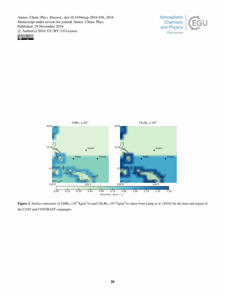
Figure 3 shows the spatial distribution of CHBr3 and CH2Br2 emissions that we use (Liang et al., 2010). These emissions

are "top-down" estimates derived from airborne measurements in the troposphere and lower stratosphere in the Western Pacific

and North America. We use de-seasonalised monthly prior emissions from this inventory, with global annual totals of 42515

Gg Br yr−1 for CHBr3 and 57 Gg Br yr−1 for CH2Br2, and impose a monthly seasonal cycle at latitudes >30◦N, following

Parrella et al. (2012).

For model evaluation using the NOAA data, described above, we initialize the model in January 2004 with near-zero values

until January 2013 with the first year discarded to minimize the impact of the initial conditions. For CAST/CONTRAST data,

we initialize the tagged tracers in January 2014 with near-zero values, and background initial conditions that were determined20

from a 12-month integration of the full-chemistry model that are subject only to atmospheric transport and loss processes. This

approach minimizes any additional model error that has accumulated during the longer model integration. We sample at the

time and location of each observation. For the NOAA data described above, we calculate monthly mean statistics from 1st

January 2005–31 December 2011.

3.2 Physical age of air model calculation25

We use the age of air simulation to understand the role and frequency of rapid convective systems to transport short-lived

halogenated compounds to the TTL, in the absence of reliable bottom-up emission inventories.

We use the GEOS-Chem to determine the physical age of air A, building on previous studies (Finch et al., 2014), and use a

consistent set of geographical regions used in our tagged CHBr3 and CH2Br2 simulations as described above.

For each model tracer (Xi) we define a surface boundary condition B that linearly increases with time t so that smaller30

values correspond to older physical ages: B = f × t×Rx, where f is a scaling factor (1×10−15 s−1), and Rx denotes the

fraction of the grid box relevant to a particular tagged tracer. We sample the resulting 3-D field of model tracers at the time

and location of CAST and CONTRAST measurements. We initialise this model in July 2013 and run for 6 months until the

start of January 2014 so that at least one e-folding lifetime of CH2Br2 has been achieved. The physical age of a tracer i since

5


it first touched a land or ocean surface is calculated as Ai = ti−Xi/f . By using the atmospheric transport model we take into

account atmospheric dispersion. We do not take into account any chemical loss in this simulation.

To explicitly evaluate marine convection in GEOS-Chem we developed a short-lived tagged tracer with an e-folding lifetime

of four days, comparable to that of methyl iodide (CH3I) in the tropics (Carpenter et al., 2014). We emit the tracer with an

equilibrium mole fraction of 1 pptv over all oceanic regions described in Figure 2. We initialise the model on 1st January 20145

with an empty 3-D atmospheric field and run for two months until 01/03/2014. Model output is archived every two hours and

the model is sampled along the aircraft flight tracks. GEOS-Chem captures mean marine convective flow over the study region

compared to CH3I observations. It also captures infrequent fast, large-scale convective transport with upper tropospheric ages

of 3–5 days, but misses small-scale variations due to rapid convection. Results are explained in detail in Appendix B.

4 Results10

4.1 Model Evaluation

We evaluate our tagged model of atmospheric CHBr3 and CH2Br2 using NOAA surface data, and CAST and CONTRAST

aircraft data during January and February 2014.

Evaluation using the NOAA data is described in Appendix A. In brief, the model generally has a positive bias but reproduces

30–60% of the seasonal variation, depending on geographical location. Model errors in reproducing the observed seasonal cycle15

reflect errors in production and loss rates. The model generally has less skill at reproducing observations collected at coastal

sites close to emission sources.

Figure 4 compares modelled and observed CHBr3 and CH2Br2. It shows that GEOS-Chem has a 30% percentage bias

for both gases during CAST and CONTRAST, which we calculate using: 100/Ni

∑i(modeli− obsi)/(max(modi,obsi)).

We assume this bias is due primarily to errors in prior emission and remove it from subsequent calculations. We find that20

the model can reproduce more than 30% of the observed variability of CHBr3 from CAST and CONTRAST and between

15% (CAST) and 45% (CONTRAST) of the observed variability of CH2Br2. In general, GEOS-Chem has poorer skill at

reproducing observed near-surface variations, reflecting errors in prior emissions. We find that the frequency distribution of the

model minus observation residuals are similar for CAST and CONTRAST but with an offset from zero, reflecting a systematic

error that is likely due to an error in prior emissions. Differences between CAST and CONTRAST reflect the bias towards25

boundary-layer sampling during CAST where measurements are more sensitive to fresh surface emissions. There are smaller

differences between CAST and CONTRAST for CH2Br2. It has a longer chemical lifetime making it comparable with the

mean mole fraction associated with the troposphere.

4.2 Tagged-VSLS model output

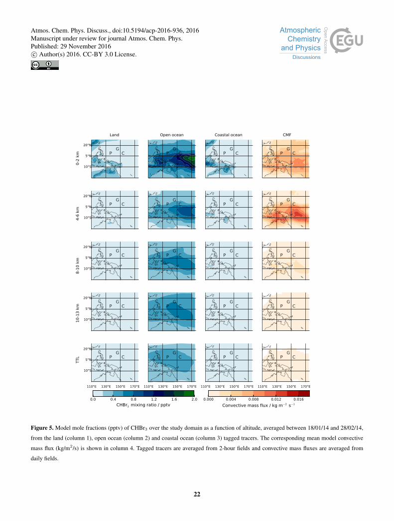
Figures 5 (Figure 6) show mean land, and open and coastal ocean tagged CHBr3 (CH2Br2) tracers over altitude compared to30

model convective mass flux. There is a strong region of convection south of Chuuk and along the equator that transports gases

6


directly from open oceanic emission sources to the mid-troposphere. Above the mid-troposphere (10 km) the mean convective

mass fluxes get smaller with gases being dissipated progressively more in the horizontal. As we show below this leads to an

inverted ‘S’ shape in the vertical profiles of CHBr3 and CH2Br2, which is observed by both campaigns (Harris et al., 2016; Pan

et al., 2016). There is also a strong convection region west of Papua New Guinea/north of Australia, close to land and coastal

emissions.5

The model shows CHBr3 mean mole fractions of 2 ppt throughout the boundary layer (0–2 km) emitted from open ocean

emissions, but deplete quickly over the vertical profile due to their short atmospheric lifetime. Throughout the TTL, mean

CHBr3 mole fractions range 0.2–0.6 ppt over the study domain and campaign period mainly due to open ocean emissions.

Coastal emissions are typically much larger than open ocean emissions but they play a much smaller role in observed variations

throughout the troposphere despite coinciding with the strong convective regions over Papua New Guinea/north of Australia.10

Prevailing easterly transport of gases over the region is dominated by the vast area of open ocean sources that appear to weaken

the magnitude of spatially limited coastal emissions (Andrews et al., 2016; Pan et al., 2016). Averaged over the campaign,

coastal and terrestrial sources of CHBr3 show little influence above 6 km. The vertical and spatial distribution of CH2Br2 mole

fractions is consistent with CHBr3 although they deplete less rapidly with altitude by virtue of their longer atmospheric lifetime.

At the TTL, averaged over the campaign study, CH2Br2 mole fractions range 0.1–0.3 ppt mainly due to smaller magnitude of15

ocean emissions compared to CHBr3. Coastal and terrestrial sources contribute up to 0.1 ppt of CH2Br2 in the TTL.

Figure 7 shows percentage contributions of geographical tracers to CAST and CONTRAST CHBr3 observations. Ocean

emissions provide the largest fractional contribution to CHBr3 during CAST, typically more than 70% throughout the low

to mid troposphere of which 60–80% is from the open ocean. Coastal ocean and land emissions represent a much smaller

contribution to CHBr3 at lower altitudes, but increase their influence above 6 km in the CONTRAST data with contributions20

from geographical regions immediately outside the study region reaching a maximum of 20% of the total CHBr3 tracer in the

TTL. This is represented in the inverted ‘S’ shape observed over the vertical profile, as mentioned above. This reflects deep

convection of air masses over the region, which has only a small amount of detrainment in the mid-troposphere followed by

advection of these air masses in the upper troposphere. Island land masses generally represent a minor contribution through

the vertical profile and we have excluded them from further analysis.25

Figure 8 shows the same as Figure 7 but for CH2Br2. The largest contributions to total CH2Br2 over the campaign period are

from the oceans, particularly from the open ocean. They typically represent 20% of the total CH2Br2 and reaching a maximum

of 34% in the TTL for the CONTRAST measurements. Maximum contributions of coastal emission sources peak at 5% of

total CH2Br2 tracer in the TTL, much less than for CHBr3. The remaining contributions are representative of emissions before

the campaign period. The longer lifetime of CH2Br2 mean that these mole fractions have a greater influence over the campaign30

profile compared to CHBr3.

4.3 Physical Age of Air

Figure 9 shows how the probability density of the age of air, A, from different geographical tracers changes over altitude.

The age of air has a bi-modal distribution peaking at approximately 60 days and 200 days. The younger age distribution is

7


dominated by air lofted over the open ocean, while the older age distribution is dominated by air lofted over the land and

coastal oceans. At progressively higher altitude regions the distributions generally age, as expected, but above the boundary

layer the median values of both modes remain relatively constant at approximately 70 days and 210 days, respectively. The

older peak is representative of emission sources have been imported into the study region from outside the study domain.

Contributions from coastal ocean and terrestrial emissions are small compared to the contribution from the larger area of5

open ocean emissions. The oldest ages, which approach the time of the study period, reflect the accumulation of near-zero

mole fractions. At higher altitudes we find that the probability distributions become less smooth, reflecting more variation in

ages. At these altitudes we also find a progressively larger (but still minor) contribution from coastal emissions. We using our

CH3I-like tracer that air masses can be transported to the TTL within 3–5 days but these are infrequent events (Appendix B).

Assuming an indicative e-folding atmospheric lifetime τ of 24 days for CHBr3 and 123 days for CH2Br2 we find that the10

majority of air lofted over the ocean has an age within 3τCHBr3 and 1τCH2Br2 . We find that 11% (52%) of oceanic emissions

reach the TTL within 2τCHBr3 (3τCHBr3 ) of which 53.6% (34.9%) are from the open oceans. Contributions from the land

and coastal oceans are negligible as they dominate the older age profile throughout the vertical. Coastal based emissions show

some influence at higher altitudes due to the difference in entire ocean and open ocean age profiles, but they have no strength

as an individual geographical tracer. The corresponding statistics for CH2Br2 are 95% of air lofted over the ocean reaches the15

TTL within 1τCH2Br2 of which 88% is lofted over the open ocean.

Figure 10 is the same as Figure 9 but sampled along CAST and CONTRAST flight tracks. The atmospheric sampling

adopted by the CAST and CONTRAST campaigns capture the bi-modal distribution of physical ages discussed above. Despite

intensive measurements around coastal land masses of the region, CAST did not very well capture coastal emissions. We also

find that CONTRAST generally better samples both modes of the distribution, reflecting the more extensive horizontal and20

vertical sampling domain and the larger number of collected measurements.

Figure 11 is the distribution of oceanic CHBr3 mixing ratios in the troposphere, in all systems and in only the highest

convective systems compared with associated age. Throughout the troposphere, CHBr3 mole fractions generally decrease with

age. The only exception is at the near-surface where land emissions dominate the older age profile. Within the TTL, the

highest CHBr3 mole fractions are associated with the youngest age of air (24–48 days), but this represents only 5% of the air25

transported to the TTL. The peak frequency for the mean age of air is 48–72 days, corresponding to 3τCHBr3 and median

values of 0.5 pptv CHBr3 from oceanic emission sources. The highest values of model convective mass flux do not account

for all the high CHBr3 mole fractions within the TTL. Less than 0.5% (2%) of air being transported to the TTL within 20–40

(48–72) days of emission are associated with high convection events. Weaker, mean convection plays an important role in more

consistently transporting large mole fractions to the free troposphere that is then transported more slowly to the TTL.30

To estimate the mean observed transport of CHBr3 and CH2Br2 to the TTL we remove the calculated model bias as described

above in section 4.1. Figure 12 shows the resulting corrected mean vertical profiles. We calculate the uncertainties using

the upper and lower limits of the bias correction, which are based on CHBr3 and CH2Br2 data that are ±2 mean absolute

deviations from the observed mean mole fractions. For CHBr3 and CH2Br2 we find biases that range -8%–80% and 19%–

43%, respectively, which we then apply to the model values throughout the atmosphere over the campaign period. We find35

8


that resulting mean model values underestimate observed CHBr3 and CH2Br2 between 9–12 km, above the main region of

convective outflow, with the observations inside the model uncertainty with the exception of CH2Br2. Mean model values

within the TTL (above 13 km and below the local tropopause) reproduce mean observations. Based on this bias correction

approach we infer a mean mole fraction and range of 0.46 (0.13–0.72) ppt and 0.88 (0.71–1.01) ppt of CHBr3 and CH2Br2

being transported to the TTL during January and February, 2014. This is consistent with a contribution of 3.14 (1.81–4.18) pptv5

of Br to the TTL Bry budget over the region of the campaign. This is consistent with Navarro et al. (2015) which estimates

VSLS contribution over the Pacific from observations in 2013 and 2014. It estimates 3.27±0.47 pptv of bromine from CHBr3,

CH2Br2 and other minor VSLS sources at the tropopause level (17 km).

Based on average observed surface values of CHBr3 (1.13 ppt) and CH2Br2 (1.02 ppt) over the campaign we infer that 40%

and 86% of these emitted gases, respectively, are directly injected into the TTL over our study domain. The larger percentage10

for CH2Br2 is consistent with its longer lifetime. Our value of 40% for the CHBr3 SGI falls within previously reported values

that range 15%–76% (median '50%) (Sinnhuber and Folkins, 2006; Hossaini et al., 2010; Tegtmeier et al., 2012; Aschmann

and Sinnhuber, 2013), but is lower than the associated median value. One possible reason for the negative bias in our SGI

estimate for CHBr3 is the bias correction approach we adopted for our analysis. Our bias correction is simple but not does take

account for vertical variations in atmospheric transport. We calculated a mean atmospheric bias, but clearly the model bias is15

much larger at lower altitudes, reflecting errors in emission estimates. However, we find that model bias at altitudes >10 km

(29%) is comparable to the bias calculated using all data (31%). There is much less vertical variation in bias for CH2Br2

because of its longer atmospheric lifetime.

5 Discussion and Concluding Remarks

We used the GEOS-Chem chemistry transport model to interpret mole fraction measurements of CHBr3 and CH2Br2 over the20

Western Pacific during the CAST and CONTRAST campaigns, January–February 2014. We found that the model reproduced

30% of CHBr3 measurements and 15% (45%) CAST (CONTRAST) CH2Br2, but had a mean positive bias of 30% for both

compounds. CAST mainly sampled the marine boundary layer (70% of observations) so that biases in prior surface emissions

have a greater influence on CAST than CONTRAST, which sampled throughout the troposphere.

To interpret the CAST and CONTRAST measurements of CHBr3 and CH2Br2 we developed two new GEOS-Chem model25

simulations: 1) a linearised tagged simulation so that we could attribute observed changes to individual sources and geo-

graphical regions, and 2) an age of air simulation to improve understanding of the vertical transport of these compounds,

acknowledging that more conventional photochemical clocks are difficult to use without more accurate boundary conditions

provided by surface emission inventories.

We have three main conclusions. First, we found that open ocean emissions of CHBr3 and CH2Br2 are primarily responsible30

for observed atmospheric mole fractions of these gases over the Western Pacific. Emissions from open ocean sources represent

up to 75% of total CHBr3, with the largest fractional contribution in the lower troposphere. Coastal ocean and terrestrial sources

typically contribute 7% to total atmospheric CHBr3 but reach a maximum of 20% in the TTL due to advection of air masses

9


convected from areas outside the study region. Based on this model interpretation, we infer that CAST observations of CHBr3,

which are mainly in the lower troposphere, are dominated by open ocean sources. In contrast, CONTRAST measurements

have a mix of sources, including a progressively larger contribution from coastal ocean and terrestrial sources in the upper

troposphere. Tropospheric measurements of CH2Br2, which has a longer atmospheric lifetime than CHBr3, are dominated by

sources from before the campaign. The open ocean source typically represents only 20% of the observed variations of CH2Br25

emitted during the campaign region throughout the troposphere.

Second, using our age of air simulation, we find that the highest CHBr3 and CH2Br2 mole fractions in the TTL correspond

to the youngest air masses being transported from oceanic sources, predominantly the open ocean. Within the TTL, the highest

CHBr3 mole fractions are associated with the youngest age of air (24–48 days), but this represents only 5% of the air transported

to the TTL. Weaker, slower convection processes are responsible for consistently transporting higher mole fractions to the UT10

and TTL. The majority of air (40%) is being transported to the TTL is within 3τCHBr3 (48–72 days) corresponding to lower

mole fractions and the majority of weaker convection events.

And third, we estimated the flux of CHBr3 and CH2Br2 to the TTL using model data that have been corrected for bias. We

calculated a mean and range of values 0.46 (0.13–0.72) pptv and 0.88 (0.71–1.01) pptv for CHBr3 and CH2Br2, respectively,

which represent 40% and 86% of estimated surface emissions. Together, they correspond to a total of 3.14 (1.81–4.18) pptv Br15

to the TTL. Our flux estimate for CHBr3 is lower than previous studies that have reported values closer to 50%.

Acknowledgements. R.B. and P.I.P. designed the computation experiments and R.B. conducted the experiment with contributions from L.F.

about the tagged model. R.B. and P.I.P. wrote the manuscript. We are grateful to the Harvard University GEOS-Chem group who maintain

the model. R.B. was funded by the United Kingdom Natural Environmental Research Council (NERC) studentship NE/1528818/1, L.F.

was funded by NERC grant NE/J006203/1, and P.I.P. gratefully acknowledges his Royal Society Wolfson Research Merit Award. R.S.20

acknowledges support from the U.S. National Science Foundation (NSF). E.A. acknowledges support from NSF Grant AGS1261689 and

thanks R. Lueb, R. Hendershot, X. Zhu, M. Navarro, and L. Pope for technical and engineering support. CAST is funded by NERC and STFC,

with grants NE/ I030054/1 (lead award), NE/J006262/1, 472 NE/J006238/1, NE/J006181/1, NE/J006211/1, NE/J006061/1, NE/J006157/1,

NE/J006203/1, NE/J00619X/1 (UoYork CAST measurements), and NE/J006173/1. The CONTRAST experiment is sponsored by the NSF.

CONTRAST data are publicly available for all researchers and can be obtained at http://data.eol.ucar.edu/master_list/?project=CONTRAST.25

The NOAA surface data is available at http://www.esrl.noaa.gov/gmd/dv/ftpdata.html.

10


References

Andrews, S. J., Carpenter, L. J., Apel, E. C., Atlas, E., Donets, V., Hopkins, J. F., Hornbrook, R. S., Lewis, A. C., Lidster, R. T., Lueb,

R., Minaeian, J., Navarro, M., Punjabi, S., Riemer, D., and Schauffler, S.: A comparison of very short-lived halocarbon (VSLS) and

DMS aircraft measurements in the Tropical West Pacific from CAST, ATTREX and CONTRAST, Atmospheric Measurement Techniques

Discussions, 2016, 1–23, doi:10.5194/amt-2016-94, http://www.atmos-meas-tech-discuss.net/amt-2016-94/, 2016.5

Aschmann, J. and Sinnhuber, B.-M.: Contribution of very short-lived substances to stratospheric bromine loading: uncertainties and con-

straints, Atmos. Chem. Phys., 13, 1203–1219, doi:10.5194/acp-13-1203-2013, http://www.atmos-chem-phys.net/13/1203/2013/, 2013.

Aschmann, J., Sinnhuber, B. M., Atlas, E. L., and Schauffler, S. M.: Modeling the transport of very short-lived substances into the tropical

upper troposphere and lower stratosphere, Atmos. Chem. Phys. Discuss., 9, 18 511–18 543, doi:10.5194/acpd-9-18511-2009, http://www.

atmos-chem-phys-discuss.net/9/18511/2009/, 2009.10

Ashfold, M. J., Harris, N. R. P., Atlas, E. L., Manning, a. J., and Pyle, J. a.: Transport of short-lived species into the Tropical Tropopause

Layer, Atmos. Chem. Phys., 12, 6309–6322, doi:10.5194/acp-12-6309-2012, http://www.atmos-chem-phys.net/12/6309/2012/, 2012.

Bell, N., Hsu, L., Jacob, D. J., Schultz, M. G., Blake, D. R., Butler, J. H., King, D. B., Lobert, J. M., and Maier-Reimer, E.: Methyl iodide:

Atmospheric budget and use as a tracer of marine convection in global models, Journal of Geophysical Research: Atmospheres, 107, ACH

8–1–ACH 8–12, doi:10.1029/2001JD001151, http://dx.doi.org/10.1029/2001JD001151, 4340, 2002.15

Carpenter, L., Reimann, S., Burkholder, J., Clerbaux, C., Hall, B., Hossaini, R., Laube, J., and Yvon-Lewis, S.: Chapter 1: Update on Ozone-

Depleting Substances (ODSs) and Other Gases of Interest to the Montreal Protocol, pp. 21–125, Global Ozone Research and Monitoring

Project Report, World Meteorological Organization (WMO), 2014.

Carpenter, L. J. and Liss, P. S.: On temperate sources of bromoform and other reactive organic bromine gases, J. Geophys. Res., 105, 20 539,

doi:10.1029/2000JD900242, http://doi.wiley.com/10.1029/2000JD900242, 2000.20

Dorf, M., Butz, a., Camy-Peyret, C., Chipperfield, M. P., Kritten, L., and Pfeilsticker, K.: Bromine in the tropical troposphere and stratosphere

as derived from balloon-borne BrO observations, Atmos. Chem. Phys. Discuss., 8, 12 999–13 015, doi:10.5194/acpd-8-12999-2008, http:

//www.atmos-chem-phys-discuss.net/8/12999/2008/, 2008.

Fernandez, R. P., Salawitch, R. J., Kinnison, D. E., Lamarque, J.-F., and Saiz-Lopez, a.: Bromine partitioning in the tropical tropopause

layer: implications for stratospheric injection, Atmos. Chem. Phys. Discuss., 14, 17 857–17 905, doi:10.5194/acpd-14-17857-2014, http:25

//www.atmos-chem-phys-discuss.net/14/17857/2014/, 2014.

Finch, D. P., Palmer, P. I., and Parrington, M.: Origin, variability and age of biomass burning plumes intercepted during BORTAS-B, Atmos.

Chem. Phys. Discuss., 14, 8723–8752, doi:10.5194/acpd-14-8723-2014, http://www.atmos-chem-phys-discuss.net/14/8723/2014/, 2014.

Fueglistaler, S., Wernli, H., and Peter, T.: Tropical troposphere-to-stratosphere transport inferred from trajectory calculations, Journal of

Geophysical Research: Atmospheres, 109, n/a–n/a, doi:10.1029/2003JD004069, http://dx.doi.org/10.1029/2003JD004069, d03108, 2004.30

Fueglistaler, S., Dessler, A. E., Dunkerton, T. J., Folkins, I., Fu, Q., and Mote, P. W.: Tropical tropopause layer, Rev. Geophys., 47, RG1004,

doi:10.1029/2008RG000267, http://doi.wiley.com/10.1029/2008RG000267, 2009.

Gettelman, a. and Forster, P. M. D. F.: A Climatology of the Tropical Tropopause Layer., J. Meteorol. Soc. Japan, 80, 911–924,

doi:10.2151/jmsj.80.911, http://joi.jlc.jst.go.jp/JST.JSTAGE/jmsj/80.911?from=CrossRef, 2002.

Gettelman, A., Salby, M. L., and Sassi, F.: Distribution and influence of convection in the tropical tropopause region, J. Geophys. Res., 107,35

4080, doi:10.1029/2001JD001048, http://doi.wiley.com/10.1029/2001JD001048, 2002.

11


Harris, N. R. P., Carpenter, L. J., Lee, J. D., Vaughan, G., Filus, M. T., Jones, R. L., OuYang, B., Pyle, J. A., Robinson, A. D., Andrews, S. J.,

Lewis, A. C., Minaeian, J., Vaughan, A., Dorsey, J. R., Gallagher, M. W., Breton, M. L., Newton, R., Percival, C. J., Ricketts, H. M. A.,

Baugitte, S. J.-B., Nott, G. J., Wellpott, A., Ashfold, M. J., Flemming, J., Butler, R., Palmer, P. I., Kaye, P. H., Stopford, C., Chemel,

C., Boesch, H., Humpage, N., Vick, A., MacKenzie, A. R., Hyde, R., Angelov, P., Meneguz, E., and Manning, A. J.: Co-ordinated

Airborne Studies in the Tropics (CAST), Bulletin of the American Meteorological Society, 0, null, doi:10.1175/BAMS-D-14-00290.1,5

http://dx.doi.org/10.1175/BAMS-D-14-00290.1, 2016.

Hossaini, R., Chipperfield, M. P., Monge-Sanz, B. M., Richards, N. a. D., Atlas, E., and Blake, D. R.: Bromoform and dibromomethane

in the tropics: a 3-D model study of chemistry and transport, Atmos. Chem. Phys., 10, 719–735, doi:10.5194/acp-10-719-2010, http:

//www.atmos-chem-phys.net/10/719/2010/, 2010.

Hossaini, R., Chipperfield, M. P., Feng, W., Breider, T. J., Atlas, E., Montzka, S. a., Miller, B. R., Moore, F., and Elkins, J.: The contribution10

of natural and anthropogenic very short-lived species to stratospheric bromine, Atmos. Chem. Phys., 12, 371–380, doi:10.5194/acp-12-

371-2012, http://www.atmos-chem-phys.net/12/371/2012/, 2012.

Hossaini, R., Mantle, H., Chipperfield, M. P., Montzka, S. A., Hamer, P., Ziska, F., Quack, B., Krüger, K., Tegtmeier, S., Atlas, E., Sala, S.,

Engel, A., Bönisch, H., Keber, T., Oram, D., Mills, G., Ordóñez, C., Saiz-Lopez, A., Warwick, N., Liang, Q., Feng, W., Moore, F., Miller,

B. R., Marécal, V., Richards, N. A. D., Dorf, M., and Pfeilsticker, K.: Evaluating global emission inventories of biogenic bromocarbons,15

Atmos. Chem. Phys., 13, 11 819–11 838, doi:10.5194/acp-13-11819-2013, http://www.atmos-chem-phys.net/13/11819/2013/, 2013.

Jones, D. B. A., Bowman, K. W., Palmer, P. I., Worden, J. R., Jacob, D. J., Hoffman, R. N., Bey, I., and Yantosca, R. M.: Potential of

observations from the Tropospheric Emission Spectrometer to constrain continental sources of carbon monoxide, Journal of Geophysical

Research: Atmospheres, 108, n/a–n/a, doi:10.1029/2003JD003702, http://dx.doi.org/10.1029/2003JD003702, 4789, 2003.

Ko, M. and Poulet, G.: Chapter 2: Very short-lived halogen and sulfur substances, in: Scientific Assessment of Ozone Depletion: 2002 Global20

Ozone Research and Monitoring Project, Report No. 47, Geneva, Switzerland, 2003.

Liang, Q., Stolarski, R. S., Kawa, S. R., Nielsen, J. E., Douglass, A. R., Rodriguez, J. M., Blake, D. R., Atlas, E. L., and Ott, L. E.: Finding

the missing stratospheric Bry: a global modeling study of CHBr3 and CH2Br2, Atmos. Chem. Phys., 10, 2269–2286, doi:10.5194/acp-

10-2269-2010, http://www.atmos-chem-phys.net/10/2269/2010/, 2010.

Liang, Q., Atlas, E., Blake, D., Dorf, M., Pfeilsticker, K., and Schauffler, S.: Convective transport of very short lived bromocarbons to the25

stratosphere, Atmos. Chem. Phys., 14, 5781–5792, doi:10.5194/acp-14-5781-2014, 2014.

Mackie, A. R., Palmer, P. I., Barlow, J. M., Finch, D. P., Novelli, P., and Jaegl’e, L.: Reduced Arctic air pollution due to decreasing Eu-

ropean and North American emissions, Journal of Geophysical Research: Atmospheres, 121, 8692–8700, doi:10.1002/2016JD024923,

2016JD024923, 2016.

McLinden, C. A., Haley, C. S., Lloyd, N. D., Hendrick, F., Rozanov, A., Sinnhuber, B.-M., Goutail, F., Degenstein, D. A., Llewellyn,30

E. J., Sioris, C. E., Van Roozendael, M., Pommereau, J. P., Lotz, W., and Burrows, J. P.: Odin/OSIRIS observations of strato-

spheric BrO: Retrieval methodology, climatology, and inferred Bry, Journal of Geophysical Research: Atmospheres, 115, n/a–n/a,

doi:10.1029/2009JD012488, http://dx.doi.org/10.1029/2009JD012488, d15308, 2010.

Montzka, S. A., Krol, M., Dlugokencky, E., Hall, B., Jöckel, P., and Lelieveld, J.: Small Interannual Variability of Global Atmospheric

Hydroxyl, Science, 331, 67–69, doi:10.1126/science.1197640, http://science.sciencemag.org/content/331/6013/67, 2011.35

Navarro, M. A., Atlas, E. L., Saiz-Lopez, A., Rodriguez-Lloveras, X., Kinnison, D. E., Lamarque, J.-F., Tilmes, S., Filus, M., Harris, N.

R. P., Meneguz, E., Ashfold, M. J., Manning, A. J., Cuevas, C. A., Schauffler, S. M., and Donets, V.: Airborne measurements of organic

12


bromine compounds in the Pacific tropical tropopause layer, Proceedings of the National Academy of Sciences, 112, 13 789–13 793,

doi:10.1073/pnas.1511463112, http://www.pnas.org/content/112/45/13789.abstract, 2015.

Ordóñez, C., Lamarque, J.-F., Tilmes, S., Kinnison, D. E., Atlas, E. L., Blake, D. R., Sousa Santos, G., Brasseur, G., and Saiz-Lopez, a.:

Bromine and iodine chemistry in a global chemistry-climate model: description and evaluation of very short-lived oceanic sources, Atmos.

Chem. Phys., 12, 1423–1447, doi:10.5194/acp-12-1423-2012, http://www.atmos-chem-phys.net/12/1423/2012/, 2012.5

Palmer, P. I., Jacob, D. J., Jones, D. B. A., Heald, C. L., Yantosca, R. M., Logan, J. A., Sachse, G. W., and Streets, D. G.: Inverting

for emissions of carbon monoxide from Asia using aircraft observations over the western Pacific, Journal of Geophysical Research:

Atmospheres, 108, n/a–n/a, doi:10.1029/2003JD003397, http://dx.doi.org/10.1029/2003JD003397, 8828, 2003.

Pan, L. L., Paulik, L. C., Honomichl, S. B., Munchak, L. A., Bian, J., Selkirk, H. B., and Vömel, H.: Identification of the tropical

tropopause transition layer using the ozone-water vapor relationship, Journal of Geophysical Research: Atmospheres, 119, 3586–3599,10

doi:10.1002/2013JD020558, http://dx.doi.org/10.1002/2013JD020558, 2013JD020558, 2014.

Pan, L. L., Atlas, E. L., Salawitch, R. J., Honomichl, S. B., Bresch, J. F., Randel, W. J., Apel, E. C., Hornbrook, R. S., Weinheimer, A. J.,

Anderson, D. C., Andrews, S. J., Baidar, S., Beaton, S. P., Campos, T. L., Carpenter, L. J., Chen, D., Dix, B., Donets, V., Hall, S. R.,

Hanisco, T. F., Homeyer, C. R., Huey, L. G., Jensen, J. B., Kaser, L., Kinnison, D. E., Koenig, T. K., Lamarque, J.-F., Liu, C., Luo,

J., Luo, Z. J., Montzka, D. D., Nicely, J. M., Pierce, R. B., Riemer, D. D., Robinson, T., Romashkin, P., Saiz-Lopez, A., Schauffler,15

S., Shieh, O., Stell, M. H., Ullmann, K., Vaughan, G., Volkamer, R., and Wolfe, G.: The Convective Transport of Active Species in

the Tropics (CONTRAST) Experiment, Bulletin of the American Meteorological Society, 0, null, doi:10.1175/BAMS-D-14-00272.1,

http://dx.doi.org/10.1175/BAMS-D-14-00272.1, 2016.

Parrella, J. P., Jacob, D. J., Liang, Q., Zhang, Y., Mickley, L. J., Miller, B., Evans, M. J., Yang, X., Pyle, J. a., Theys, N., and Van Roozendael,

M.: Tropospheric bromine chemistry: implications for present and pre-industrial ozone and mercury, Atmos. Chem. Phys., 12, 6723–6740,20

doi:10.5194/acp-12-6723-2012, http://www.atmos-chem-phys.net/12/6723/2012/, 2012.

Quack, B. and Wallace, D. W. R.: Air-sea flux of bromoform: Controls, rates, and implications, Global Biogeochem. Cycles, 17, 23 1–27,

doi:10.1029/2002GB001890, http://doi.wiley.com/10.1029/2002GB001890, 2003.

Quack, B., Atlas, E., Petrick, G., and Wallace, D. W. R.: Bromoform and dibromomethane above the Mauritanian upwelling: Atmo-

spheric distributions and oceanic emissions, J. Geophys. Res., 112, D09 312, doi:10.1029/2006JD007614, http://doi.wiley.com/10.1029/25

2006JD007614, 2007.

Salawitch, R. J., Canty, T., Kurosu, T., Chance, K., Liang, Q., da Silva, A., Pawson, S., Nielsen, J. E., Rodriguez, J. M., Bhartia, P. K., Liu,

X., Huey, L. G., Liao, J., Stickel, R. E., Tanner, D. J., Dibb, J. E., Simpson, W. R., Donohoue, D., Weinheimer, A., Flocke, F., Knapp,

D., Montzka, D., Neuman, J. A., Nowak, J. B., Ryerson, T. B., Oltmans, S., Blake, D. R., Atlas, E. L., Kinnison, D. E., Tilmes, S.,

Pan, L. L., Hendrick, F., Van Roozendael, M., Kreher, K., Johnston, P. V., Gao, R. S., Johnson, B., Bui, T. P., Chen, G., Pierce, R. B.,30

Crawford, J. H., and Jacob, D. J.: A new interpretation of total column BrO during Arctic spring, Geophysical Research Letters, 37,

n/a–n/a, doi:10.1029/2010GL043798, http://dx.doi.org/10.1029/2010GL043798, l21805, 2010.

Sander, S., Friedl, R., Barker, J., Golden, D., Kurylo, M., Wine, P., Abbatt, J., Burkholder, J., Kolb, C., Moortgat, G., Huie, R., and Orkin, V.:

Chemical Kinetics and Photochemical Data for Use in Atmospheric Studies, Evaluation Number 17, JPL Publication 10–6, Jet Propulsion

Laboratory, http://jpldataeval.jpl.nasa.gov, 2011.35

Sinnhuber, B.-M. and Folkins, I.: Estimating the contribution of bromoform to stratospheric bromine and its relation to dehydration in the

tropical tropopause layer, Atmos. Chem. Phys., 6, 4755–4761, doi:10.5194/acp-6-4755-2006, http://www.atmos-chem-phys.net/6/4755/

2006/, 2006.

13


Sinnhuber, B.-M., Arlander, D. W., H, B., Burrows, J. P., Chipperfield, M. P., Enell, C.-F., Frieb, U., Hendrick, F., Johnston, P. V., Jones, R. L.,

Kreher, K., Mohamed-Tahrin, N., Muller, R., Pfeilsticker, K., Platt, U., Pommereau, J.-P., Pundt, I., Richter, A., South, A. M., Tornkvist,

K. K., Van Roozendael, M., Wagner, T., and Wittrock, F.: Comparison of measurements and model calculations of stratospheric bromine

monoxide, J. Geophys. Res., 107, 4398, doi:10.1029/2001JD000940, http://doi.wiley.com/10.1029/2001JD000940, 2002.

Sinnhuber, B.-M., Rozanov, A., Sheode, N., Afe, O. T., Richter, A., Sinnhuber, M., Wittrock, F., Burrows, J. P., Stiller, G. P., von Clarmann, T.,5

and Linden, A.: Global observations of stratospheric bromine monoxide from SCIAMACHY, Geophysical Research Letters, 32, n/a–n/a,

doi:10.1029/2005GL023839, http://dx.doi.org/10.1029/2005GL023839, l20810, 2005.

Sioris, C. E., Kovalenko, L. J., McLinden, C. A., Salawitch, R. J., Van Roozendael, M., Goutail, F., Dorf, M., Pfeilsticker, K., Chance, K., von

Savigny, C., Liu, X., Kurosu, T. P., Pommereau, J.-P., Bösch, H., and Frerick, J.: Latitudinal and vertical distribution of bromine monoxide

in the lower stratosphere from Scanning Imaging Absorption Spectrometer for Atmospheric Chartography limb scattering measurements,10

Journal of Geophysical Research: Atmospheres, 111, n/a–n/a, doi:10.1029/2005JD006479, http://dx.doi.org/10.1029/2005JD006479,

d14301, 2006.

Tegtmeier, S., Krüger, K., Quack, B., Atlas, E. L., Pisso, I., Stohl, a., and Yang, X.: Emission and transport of bromocarbons: from

the West Pacific ocean into the stratosphere, Atmos. Chem. Phys., 12, 10 633–10 648, doi:10.5194/acp-12-10633-2012, http://www.

atmos-chem-phys.net/12/10633/2012/, 2012.15

Warwick, N. J., Pyle, J. a., Carver, G. D., Yang, X., Savage, N. H., O’Connor, F. M., and Cox, R. a.: Global modeling of biogenic bromocar-

bons, J. Geophys. Res., 111, D24 305, doi:10.1029/2006JD007264, http://doi.wiley.com/10.1029/2006JD007264, 2006.

WMO: Scientific Assessment of Ozone Depletion: 2006, Global Ozone Research and Monitoring Project - Report No. 50, 572pp., Tech.

rep., Geneva, 2007.

Zhou, X. L., Geller, M. A., and Zhang, M.: Temperature Fields in the Tropical Tropopause Transition Layer, Journal of Climate, 17, 2901–20

2908, doi:10.1175/1520-0442(2004)017<2901:TFITTT>2.0.CO;2, http://dx.doi.org/10.1175/1520-0442(2004)017<2901:TFITTT>2.0.

CO;2, 2004.

Ziska, F., Quack, B., Abrahamsson, K., Archer, S. D., Atlas, E., Bell, T., Butler, J. H., Carpenter, L. J., Jones, C. E., Harris, N. R. P., Hepach,

H., Heumann, K. G., Hughes, C., Kuss, J., Krüger, K., Liss, P., Moore, R. M., Orlikowska, a., Raimund, S., Reeves, C. E., Reifenhäuser,

W., Robinson, a. D., Schall, C., Tanhua, T., Tegtmeier, S., Turner, S., Wang, L., Wallace, D., Williams, J., Yamamoto, H., Yvon-Lewis,25

S., and Yokouchi, Y.: Global sea-to-air flux climatology for bromoform, dibromomethane and methyl iodide, Atmos. Chem. Phys., 13,

8915–8934, doi:10.5194/acp-13-8915-2013, http://www.atmos-chem-phys.net/13/8915/2013/, 2013.

14


Table 1. Mean measurement statistics for CHBr3 and CH2Br2 mole fraction data as a function of altitude for CAST and CONTRAST aircraft

campaigns. x, σ, and n denote the mean value, the standard deviation, and the number of data points used to determine the statistics.

Altitude CHBr3 CH2Br2

CAST CONTRAST CAST CONTRAST

km x, 1σ, & range [ppt]; n x, 1σ, & range [ppt]; n x, 1σ, & range [ppt] x, 1σ, & range [ppt]

0−2 0.95, 0.45, 0.42−3.00; 502 0.89, 0.23, 0.51−1.55; 75 1.01, 0.13, 0.72−1.64 1.07, 0.11, 0.83−1.27

2−4 0.61, 0.16, 0.29−0.98; 147 0.62, 0.18, 0.29−1.24; 48 0.91, 0.05, 0.73−1.06 0.94, 0.09, 0.78−1.13

4−6 0.44, 0.17, 0.03−0.79; 59 0.56, 0.18, 0.20−1.12; 65 0.88, 0.06, 0.69−1.00 0.91, 0.09, 0.73−1.12

6−8 0.38, 0.25, 0.02−0.81, 53 0.60, 0.20, 0.24−1.01; 43 0.85, 0.11, 0.63−1.06 0.90, 0.10, 0.70−1.06

8−10 0.48, 0.34, 0.14−0.82; 2 0.62, 0.17, 0.24−1.00; 43 0.90, 0.13, 0.77−1.03 0.93, 0.09, 0.72−1.07

10−13 – 0.59, 0.25, 0.00−1.38; 130 – 0.87, 0.19, 0.21−1.10

TTL – 0.48, 0.16, 0.18−1.17; 280 – 0.86, 0.08, 0.64−1.06

15


Table 2. Location and code of NOAA/ESRL ground-based stations. All located at the surface with exceptions of SUM (3210 m), MLO (3397

m) and SPO (2810 m).

Station Name Lat Lon

ALT Alert, NW Territories, Canada 82.5◦N 62.3◦W

SUM Summit, Greenland 72.6◦N 38.4◦W

BRW Pt. Barrow, Alaska, USA 71.3◦N 156.6◦W

MHD Mace Head, Ireland 53.0◦N 10.0◦W

LEF Wisconsin, USA 45.6◦N 90.2◦W

HFM Massachusetts, USA 42.5◦N 72.2◦W

THD Trinidad Head, USA 41.0◦N 124.0◦W

NWR Niwot Ridge, Colorado, USA 40.1◦N 105.6◦W

KUM Cape Kumukahi, Hawaii, USA 19.5◦N 154.8◦W

MLO Mauna Loa, Hawaii, USA 19.5◦N 155.6◦W

SMO Cape Matatula, American Samoa 14.3◦S 170.6◦W

CGO Cape Grim, Tasmania, Australia 40.7◦S 177.8◦E

PSA Palmer Station, Antarctica 64.6◦S 64.0◦W

SPO South Pole 90.0◦N –

16


Table 3. Seasonal break down of statistics for NOAA ground station sites (Table 2) showing r2 correlations between observed and climato-

logical monthly mean CHBr3 and CH2Br2 mole fraction data and corresponding model bias values.

CHBr3 CH2Br2

DJF MAM JJA SON DJF MAM JJA SON

Station r2, %bias r2, %bias r2, %bias r2, %bias r2, %bias r2, %bias r2, %bias r2, %bias

ALT 0.00, 3.8 0.55, 0.1 0.05, 5.5 0.43, 19.3 0.09, 12.4 0.21, 0.0 0.23, 10.0 0.31, 21.0

SUM 0.05, 25.1 0.01, –17.1 0.23, –12.0 0.54, 20.6 0.06, –2.7 0.15, –13.0 0.15, 4.8 0.60, 7.0

BRW 0.00, –41.3 0.52, –30.2 0.13, –26.5 0.80, –26.5 0.15, 9.5 0.07, –8.7 0.00, –4.4 0.14, 15.9

MHD 0.00, –40.8 0.18, –72.4 0.04, –80.6 0.08, –61.2 0.05, –20.5 0.11, –35.9 0.14, –42.7 0.03, –16.8

LEF 0.03, 45.7 0.01, 15.5 0.03, 39.3 0.73, 51.2 0.17, 13.4 0.25, 3.1 0.44, 18.2 0.66, 20.8

HFM 0.06, 52.2 0.01, 30.1 0.15, 46.9 0.38, 52.3 0.03, 20.0 0.06, 9.3 0.22, 27.1 0.45, 25.7

THD 0.19, 55.3 0.15, 15.8 0.36, 11.7 0.17, 40.2 0.09, 16.9 0.06, 0.9 0.01, 8.6 0.06, 18.0

NWR 0.02, 43.3 0.49, 25.9 0.01, 21.8 0.31, 38.7 0.20, 2.3 0.55, 4.9 0.40, 11.9 0.55, 14.7

KUM 0.00, 20.2 0.37, –1.9 0.05, 0.9 0.01, 6.8 0.25, –0.3 0.50, 4.4 0.47, 15.6 0.38, 9.9

MLO 0.18, 61.9 0.60, 60.3 0.02, 65.1 0.58, 64.7 0.14, 14.8 0.32, 15.2 0.21, 22.8 0.27, 25.0

SMO 0.23, 8.2 0.02, –4.9 0.04, 3.0 0.11, 4.7 0.39, 6.9 0.38, –0.9 0.19, –0.2 0.09, 5.6

CGO 0.23, –39.0 0.01, –12.8 0.05, 7.7 0.00, –19.6 0.13, –8.7 0.13, –1.6 0.04, –1.4 0.12, –9..5

PSA 0.19, –13.9 0.25, 26.4 0.01, 31.7 0.05, –1.9 0.00, –1.7 0.29, 11.7 0.15, 10.3 0.05, –2.0

SPO 0.50, 6.6 0.12, 6.7 0.07, 19.2 0.11, –7.3 0.01, 4.8 0.06, 4.6 0.11, 3.7 0.00, –0.6

17


G

CP

15°S

5°S

5°N

15°N

25°N

35°N

130°E 145°E 160°E 175°E

CAST

G

CP

130°E 145°E 160°E 175°E

CONTRAST

0

2

4

6

8

10

12

14

16

Alt

itude /

km

Figure 1. Distribution of measurements of CHBr3 and CH2Br2 from the CAST (left) and CONTRAST (right) aircraft campaigns as a

function of altitude (km). Relevant island waypoints are shown inset: Guam (G), Palau (P), and Chuuk (C).

18


G

CP

M

10°S

5°N

20°N

Land

G

CP

M

Ocean

G

CP

M

130°E 150°E 170°E10°S

5°N

20°N

Open ocean

G

CP

M

130°E 150°E 170°E

Coastal ocean

0.00

0.15

0.30

0.45

0.60

0.75

0.90

1.05

CH

Br 3

flu

x /

x 1

0−

13 k

g m

−1 s−

1

Figure 2. Flux of CHBr3 from land and ocean, the latter separated in to its open and coastal ocean tracers. Guam (G), Palau (P), Chuuk (C)

and Manus (M).

19


0°

15°N

30°N

120°E 145°E

Guam

ChuukPalau

CHBr3 x 1013

0°

15°N

30°N

120°E 145°E

Guam

ChuukPalau

CH2 Br2 x 1014

0.00 0.15 0.30 0.45 0.60 0.75 0.90 1.05 1.20 1.35 1.50

VSLS flux / kg m−2 s−1

Figure 3. Surface emissions of CHBr3 (1013kg/m2/s) and CH2Br2 (1014kg/m2/s) taken from Liang et al. (2010) for the time and region of

the CAST and CONTRAST campaigns.

20


0.0 0.5 1.0 1.5 2.0 2.5 3.0

Observed VSLS / pptv

0.0

0.5

1.0

1.5

2.0

2.5

3.0

Tota

l ta

gged V

SLS

/ p

ptv

r2 = 0.37r2 = 0.32

bias = +31.01%

CHBr3

0.4 0.6 0.8 1.0 1.2 1.4 1.6 1.8 2.0

Observed VSLS / pptv

0.4

0.6

0.8

1.0

1.2

1.4

1.6

1.8

2.0

r2 = 0.15r2 = 0.45

bias = +29.39%

CH2 Br2

1.0 0.5 0.0 0.5 1.0 1.5 2.0

Tagged model - observed VSLS / pptv

0.0

0.5

1.0

1.5

2.0

mean = 0.50median = 0.41


0.6 0.4 0.2 0.0 0.2 0.4 0.6 0.8 1.0


0

1

2

3

4

5



1.5 1.0 0.5 0.0 0.5 1.0 1.5 2.0


0-2

2-4

4-6

6-8

8-10

10-1212-1414-16

Alt

itude /

km

CAST CONTRAST

0.4 0.2 0.0 0.2 0.4 0.6 0.8


Figure 4. Comparisons of model and observed (left) CHBr3 and (right) CH2Br2 mole fractions from the (blue) CAST and (red) CONTRAST

aircraft campaigns. The top, middle and bottom rows display the comparison as a scatter plot (with the Pearson correlation, linear best-fit

line, and percentage bias inset); a frequency distribution of the model minus observed values; and a vertical profile of box-and-whiskers of

the model minus observed values.21


GCP

10°S

5°N

20°NG

CPG

CPG

CP

GCP

10°S

5°N

20°NG

CPG

CPG

CP

GCP

10°S

5°N

20°NG

CPG

CPG

CP

GCP

10°S

5°N

20°NG

CPG

CPG

CP

GCP

110°E 130°E 150°E 170°E

10°S

5°N

20°NG

CP

110°E 130°E 150°E 170°E

GCP

110°E 130°E 150°E 170°E

GCP

110°E 130°E 150°E 170°E

0.0 0.4 0.8 1.2 1.6 2.0

CHBr3 mixing ratio / pptv0.000 0.004 0.008 0.012 0.016

Convective mass flux / kg m−2 s−1

0-2

km

4-6

km

8-1

0 k

m1

0-1

3 k

mTTL

Land Open ocean Coastal ocean CMF

Figure 5. Model mole fractions (pptv) of CHBr3 over the study domain as a function of altitude, averaged between 18/01/14 and 28/02/14,

from the land (column 1), open ocean (column 2) and coastal ocean (column 3) tagged tracers. The corresponding mean model convective

mass flux (kg/m2/s) is shown in column 4. Tagged tracers are averaged from 2-hour fields and convective mass fluxes are averaged from

daily fields.

22


GCP

10°S

5°N

20°NG

CPG

CPG

CP

GCP

10°S

5°N

20°NG

CPG

CPG

CP

GCP

10°S

5°N

20°NG

CPG

CPG

CP

GCP

10°S

5°N

20°NG

CPG

CPG

CP

GCP

110°E 130°E 150°E 170°E

10°S

5°N

20°NG

CP

110°E 130°E 150°E 170°E

GCP

110°E 130°E 150°E 170°E

GCP

110°E 130°E 150°E 170°E

0.0 0.3 0.6 0.9 1.2

CH2 Br2 mixing ratio / pptv0.000 0.004 0.008 0.012 0.016

Convective mass flux / kg m−2 s−1

0-2

km

4-6

km

8-1

0 k

m1

0-1

3 k

mTTL

Land Open ocean Coastal ocean CMF

Figure 6. As Figure 5 but for CH2Br2.

23


0-2

2-4

4-6

6-8

8-10

10-13

TTL

Land

CAST

CONTRAST

Ocean

0 20 40 60 80 100

0-2

2-4

4-6

6-8

8-10

10-13

TTL

Open

0 20 40 60 80 100

Coastal

Percentage contribution to total CHBr3

Alt

itude /

km

Figure 7. The percentage contributions, expressed as a box and whiskers plot, from land and ocean sources to total CHBr3 sampled through-

out the troposphere during (blue) CAST and (red) CONTRAST campaigns.

24


0-2

2-4

4-6

6-8

8-10

10-13

TTL

Land

CAST

CONTRAST

Ocean

0 5 10 15 20 25 30 35

0-2

2-4

4-6

6-8

8-10

10-13

TTL

Open

0 5 10 15 20 25 30 35

Coastal

Percentage contribution to total CH2 Br2

Alt

itude /

km

Figure 8. As Figure 7 but for CH2Br2.

25


0.00

0.01

0.02

0.03

0.04

0.05

0.06

0.07

0.08

Pro

babili

ty d

ensi

ty

Mean:205.5526.1935.47212.76

0-2 km

Mean:185.7662.3573.32211.10

2-4 km

Mean:184.0968.9080.59210.40

4-6 km

Age / Days

Mean:184.7868.5581.29209.38

6-8 km

0 50 100 150 200 250Age / Days

0.00

0.01

0.02

0.03

0.04

0.05

0.06

0.07

0.08

Pro

babili

ty d

ensi

ty

Mean:186.2065.3978.91208.60

8-10 km

0 50 100 150 200 250Age / Days

Mean:187.8762.3777.16207.33

10-13 km

0 50 100 150 200 250Age / Days

Mean:188.5474.7587.59208.34

TTL

Land

Ocean

Open ocean

Coastal ocean

Figure 9. Frequency distributions of probability density function of the age of air A for (orange) land, (blue) entire ocean, and (green) open

and (black) coastal ocean tracers in 2 km altitude regions up to the TTL (13 km to the tropopause) averaged over 18/01/2014–28/02/2014.

26


0 50 100 150 200 250Age / Days

0.00

0.02

0.04

0.06

0.08

0.10

0.12

0.14

0.16

0.18

Pro

babili

ty d

ensi

ty

206.0223.2127.33212.18

Mean:

CAST

0 50 100 150 200 250Age / Days

197.2256.4966.36213.88

Mean:

CONTRAST

LandOceanOpen oceanCoastal ocean

Figure 10. As Figure 9 but sampled along CAST and CONTRAST flight tracks.

27


0

1

2

3

4

5

0-2 km 2-4 km 4-6 km 6-8 km

0-2

4

24-4

8

48-7

2

72-9

6

96-1

20

120-1

44

144-1

68

168-1

92

192-2

16

216-2

40

0

1

2

3

4

5

8-10 km

0-2

4

24-4

8

48-7

2

72-9

6

96-1

20

120-1

44

144-1

68

168-1

92

192-2

16

216-2

40

10-13 km

0-2

4

24-4

8

48-7

2

72-9

6

96-1

20

120-1

44

144-1

68

168-1

92

192-2

16

216-2

40

TTL

0

20

40

60

80

100

0

20

40

60

80

100

Age / Days

CH

Br 3

mix

ing r

ati

o /

pptv

CH

Br 3

mix

ing r

ati

o in v

ert

cal co

lum

ns

>9

5th

perc

enti

le C

MF

/ pptv

Perce

nta

ge fre

quency

of e

vents

Figure 11. Box and whiskers plot of model CHBr3 mole fractions from the entire ocean tracer as a function of 2 km altitude intervals and

nominal 24-day e-folding lifetime. Data are averaged over 18/01/2014–28/02/2014 and over 10◦S-30◦N, 125-175◦E. All data are shown in

blue and data corresponding to convective mass fluxes >95th percentile are show in red. Solid lines denotes the percentage of occurrence

rate over the period and region denoted above.

28


0.0 0.5 1.0 1.5 2.0Mean mixing ratio VSLS / pptv

0

2

4

6

8

10

12

14

16

18

Alt

itude /

km

CHBr3

CH2 Br2

Tropopause

Figure 12. Observed (solid circles) and model (dashed-dot line) mean mole fractions of CHBr3 (blue) and CH2Br2 (red) as a function

of altitude, January–February 2014. The horizontal lines associated with each mean observation denotes the range about that mean. The

coloured envelopes associated with the model denote the uncertainty based on the bias correction as described in the main text. The black

horizontal dashed line denotes the mean model tropopause of 16.5 km.

29


Appendix A: Model Evaluation Using NOAA Surface Mole Fraction Measurements

Figure A.1 is the mean annual percentage bias and associated r2 values betweens modelled and observed CHBr3 and CH2Br2

at stations in table2. The majority of station sites have a positive model bias with magnitude varying depending on location.

Mid-latitude stations (LEF–NWR) have similar bias values of 30–40% (10–20%) for CHBr3 (CH2Br2). At the tropical sites,

which are comparable with the campaign region, the model bias varies strongly depending on location. KUM and MLO both sit5

on Hawaii, with KUM and SMO being a near surface coastal station and MLO sitting at an elevated altitude of 3397 m. Model

bias calculated for MLO (60%) is much greater than the other two near surface sites (<10%), however it gives the strongest

annual correlation with r2 values of 0.75 (0.55) for CHBr3 (CH2Br2). All coastal sites (with exception of ALT) near emission

sources have low r2 values (<0.4) suggesting the model does not capture local variations in emissions well.

Seasonal variations within model bias and correlations of CHBr3 and CH2Br2 are shown in Table 3. The campaign season of10

DJF is poorly constrained within the model at all sites with an r2 < 0.5 for both gases. The annual correlation at sites appears

to be dominated by other seasons. Within the tropical stations, model bias increases from the annual at KUM to around 20%

with no correlation to observed values. MLO and SMO show a similar seasonal bias to the annual indicating the effect to be

local to the KUM station site.

Figure A.2 is the observed modelled and seasonal cycle at the tropical station sites (KUM, MLO and SMO) for CHBr315

and CH2Br2. The model is able to reproduce the seasonal cycle well at all three sites. The emissions at these sites are not

scaled seasonally, the phase is representative of the chemistry at these sites. The shorter lived CHBr3 profile is dominates by

its loss from photolysis whereas the CH2Br2 cycle is dominated by oxidation with OH. The amplitude of the seasonal cycle is

overestimated in CHBr3 at MLO, and to a lesser extent KUM. This can be indicative of local biases within photolysis loss rates

and/or emissions. The same effect is not shown within the CH2Br2 suggesting there is not a similar problem associated with20

OH fields. This is concurrent with a recent multi-decadal analysis of carbon monoxide Mackie et al. (2016) at higher northern

latitudes does not support a major problem with similar monthly 3-D fields of OH.

30


ALT

SUM

BRW

MH

D

LEF

HFM

THD

NW

R

KUM

MLO

SMO

CG

O

PSA

SPO

Station

80

60

40

20

0

20

40

60

80

Perc

enta

ge b

ias

0.0

0.2

0.4

0.6

0.8

1.0

r2 (

obse

rved v

s m

odelle

d d

ata

)

CHBr3

CH2 Br2

Figure A.1. Mean annual percentage model bias (blue) calculated at NOAA ground station sites (Table 2) for CHBr3 (dots) and CH2Br2

(crosses). The horizontal dashed line denotes zero bias. The right-hand-side y axis describes the ability of the model to reproduce observed

variations (r2) (red). The vertical dotted lines define the tropical stations.

31


0 2 4 6 8 10 12

0.6

0.4

0.2

0.0

0.2

0.4

0.6

CH

Br 3

anom

aly

/ p

ptv

KUM

0 2 4 6 8 10 12

0.4

0.2

0.0

0.2

0.4

MLO

0 2 4 6 8 10 12

0.4

0.2

0.0

0.2

0.4

SMO

0 2 4 6 8 10 12Month

0.4

0.3

0.2

0.1

0.0

0.1

0.2

0.3

0.4

CH

2B

r 2 a

nom

aly

/ p

ptv

0 2 4 6 8 10 12Month

0.4

0.3

0.2

0.1

0.0

0.1

0.2

0.3

0.4

Model Observations

0 2 4 6 8 10 12Month

0.4

0.3

0.2

0.1

0.0

0.1

0.2

0.3

0.4

a)

b)

Figure A.2. Observed (green) and model (blue) mole fractions of (a) CHBr3 and (b) CH2Br2 at tropical NOAA sites. The seasonal cycle is

shown as the climatological monthly mean anomaly calculated by subtracting the annual mean from the climatological monthly mean (pptv).

Horizontal bars on observed values denote ±1σ.

Appendix B: Evaluation of Model Convection

To evaluate model convection over the marine environment during the CAST and CONTRAST campaigns, we developed a

short-lived tagged tracer simulation with an e-folding lifetime comparable to CH3I, as described in section 3.

We emitted CH3I at an equilibrium mole fraction of 1 pptv over ocean regions and applied an atmospheric e-folding lifetime

of four days similar to that CH3I in the tropics Carpenter et al. (2014). We can then use the model mole fraction to determine5

the effective mean age of air parcels throughout the troposphere, and to compare the qualitatively to observed CH3I values

collected during the CONTRAST campaign.

Figure B.1 is a comparison of observed CH3I to our CH3I-like tracer. The model can generally reproduce the quantitative

vertical distribution of CH3I: a decrease from the surface source up to an altitude of 10–11 km. Above this, there is a 1-2 km

altitude region where values are higher than those in the free troposphere, suggestive of outflow from convection. As expected,10

32


the youngest air masses are close to the surface with the ages as young as 5–6 days in the upper troposphere. These ages are

indicative of fast convective transport but they are not as young as would be expected from some of the highest observed mole

fractions, which are likely due to faster, sub-grid scale, convective transport.

Figure B.2 is the probability distribution of the age of the simulated CH3I-like tracer between 10–15 km altitude. The model

captures infrequent fast, large-scale convective transport over the study domain, with ages as young as 3–4 days reaching5

the upper troposphere. One metric to describe the convective transport is the marine convection index (MCI), following Bell

et al. (2002): the ratio of mean upper tropospheric CH3I (8–12 km) to lower tropospheric CH3I (0–2.5 km). The CONTRAST

observations have an MCI of 0.38 and the corresponding model MCI sampled for these observations is 0.19. The MCI for the

model domain for the duration of CONTRAST is 0.28. These values are consistent with those found in Bell et al. (2002) over

a similar Pacific regions.10

Overall, we find that the model describes the mean convective flow over the region and can capture instances of rapid, large-

scale convective transport. Differences in the MCI suggest a significant role for rapid, sub-grid scale vertical transport that are

not captured by our coarse model resolution.

33


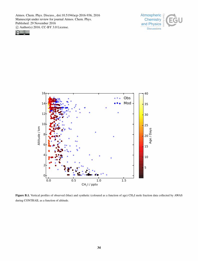
0.0 0.5 1.0 1.5CH3 I / pptv

0

2

4

6

8

10

12

14

16

Alt

itude /

km

ObsMod

5

10

15

20

25

30

35

40

Age /

Days

Figure B.1. Vertical profiles of observed (blue) and synthetic (coloured as a function of age) CH3I mole fraction data collected by AWAS

during CONTRAIL as a function of altitude.

34


0 5 10 15 20 25 30 35 40 45Age / Days

0.00

0.05

0.10

0.15

0.20

0.25

0.30All data

Plane flight

Figure B.2. Probability distribution of the physical age of CH3I for the 3-D study domain (solid line) and as sampled by the aircraft (dashed

line) between 11–15 km during CONTRAST, 18th January–28th February, 2014. The dotted line indicates 1τCH3I of 4 days.

35


Documents

Quantifying the vertical transport of CHBr and CH Br … the vertical transport of CHBr 3 and CH 2 Br 2 over the Western Pacic Robyn Butler 1, Paul I. Palmer 1, Liang Feng 1, Stephen