Embed Size (px)
Citation preview

Quadratic ProgrammingGIAN Short Course on Optimization:
Applications, Algorithms, and Computation
Sven Leyffer
Argonne National Laboratory
September 12-24, 2016

Outline
1 Introduction to Quadratic ProgrammingApplications of QP in Portfolio SelectionApplications of QP in Machine Learning
2 Active-Set Method for Quadratic ProgrammingEquality-Constrained QPsGeneral Quadratic Programs
3 Methods for Solving EQPsGeneralized Elimination for EQPsLagrangian Methods for EQPs
2 / 36

Introduction to Quadratic ProgrammingQuadratic Program (QP)
minimizex
12x
TGx + gT x
subject to aTi x = bi i ∈ EaTi x ≥ bi i ∈ I,
where
G ∈ Rn×n is a symmetric matrix... can reformulate QP to have a symmetric Hessian
E and I sets of equality/inequality constraints
Quadratic Program (QP)
Like LPs, can be solved in finite number of steps
Important class of problems:
Many applications, e.g. quadratic assignment problemMain computational component of SQP:Sequential Quadratic Programming for nonlinear optimization
3 / 36

Introduction to Quadratic Programming
Quadratic Program (QP)
minimizex
12x
TGx + gT x
subject to aTi x = bi i ∈ EaTi x ≥ bi i ∈ I,
No assumption on eigenvalues of G
If G � 0 positive semi-definite, then QP is convex⇒ can find global minimum (if it exists)
If G indefinite, then QP may be globally solvable, or not:
If AE full rank, then ∃ZE null-space basisConvex, if “reduced Hessian” positive semi-definite:
ZTE GZE � 0, where ZT
E AE = 0 then globally solvable
... eliminate some variables using the equations
4 / 36

Introduction to Quadratic Programming
Quadratic Program (QP)
minimizex
12x
TGx + gT x
subject to aTi x = bi i ∈ EaTi x ≥ bi i ∈ I,
Feasible set may be empty ... use phase-I methods from LP.
Feasible set can be unbounded ⇒ QP may be unbounded... detect during the line-search ... G � 0 implies boundedness
Polyhedral feasible set ... but solution may not be at vertex:
minimizex
x2 subject to − 1 ≤ x ≤ 1
5 / 36

Applications of QP in Portfolio Selection
Investment decisions across collection of financial assets (e.g.stocks)
Return and risk on investment are unknown (random vars)
Historical data provides
Expected rate of return of investmentCovariance of rates of returns for investments
Markowitz Investment Model
Balances risk and return (multi-objective)
Choose mix of investment
minimize risk (covariance)subject to minimum expected return
Goal: Find how much to invest in each asset
Simple model, there exist more sophisticated models
6 / 36

Applications of QP in Portfolio Selection
Problem Data
n number of available assets
r desired minimum growth of portfolio
β available capital for investment
mi expected rate of return of asset i
C covariance matrix of asset returns... models correlation between assets
Problem Variables
xi amount of investment in asset i
Assume xi ≥ 0 and xi ∈ R real
7 / 36

Applications of QP in Portfolio Selection
Problem Objective
Minimize risk of investment
minimizex
xTCx
Problem Constraints
Minimum rate of return on investment
n∑i=1
mixi ≥ r
Upper bound on total investment
n∑i=1
xi ≤ β
8 / 36

Applications of QP in Machine LearningLeast squares problem
Solve system of equations with more equations than variables
Classical problem in data fitting / regression analysis
minimizex
‖Ax − b‖22
... dates back to Legendre (1805)
Solution from normal equations or augmented system(preferred)
ATAx = ATb ⇔[
0 AT
A −I
](xu
)=
(0b
)Writing least-squares as a QP:
‖Ax − b‖22 =(Ax − b
)T (Ax − b
)= xTATAx − 2bTAx + bTb
9 / 36

Applications of QP in Machine Learning
Snag: Least-squares solution, x , typically denseInterested in sparse solution, x , with few nonzeros ⇒ `1 norm
1 LASSO: least absolute shrinkage and selection operator
minimizex
‖Ax − b‖22 subject to ‖x‖1 ≤ τ
`1-norm constraint act like a “sparsifier”Least-squares problem with limit on number of nonzeros
2 Regularized least-squares
minimizex
‖Ax − b‖22 + λ‖x‖1
Related to basis pursuit denoising`1-norm penalty act like a “sparsifier”
10 / 36

Writing LASSO as QP Problem
LASSO: least absolute shrinkage and selection operator
minimizex
‖Ax − b‖22 subject to ‖x‖1 ≤ τ
Recall `1 norm: ‖x‖1 =n∑
i=1
|xi |
vi all 2n vectors of +1,−1v0 = (1, . . . , 1), v1 = (−1, 1, . . . , 1), etc
LASSO equivalent to exponential QP
minimizex
‖Ax − b‖22subject to vTi x ≤ τ, ∀i
... QP with 2n constraints
11 / 36

Regularized Least-Squares as QP Problem
Regularized least-squares
minimizex
‖Ax − b‖22 + λ‖x‖1
Introduce variables x+i , x−i for positive/negative part of xi
Then it follows that
xi = x+i − x−i , |xi | = x+i + x−i , x+i ≥ 0, x−i ≥ 0
Regularized least-squares equivalent to
minimizex
‖Ax − b‖22 + λ(eT x+ + eT x−
)subject to x = x+ − x−
x+ ≥ 0, x− ≥ 0
where e = (1, . . . , 1)
12 / 36
Outline
1 Introduction to Quadratic ProgrammingApplications of QP in Portfolio SelectionApplications of QP in Machine Learning
2 Active-Set Method for Quadratic ProgrammingEquality-Constrained QPsGeneral Quadratic Programs
3 Methods for Solving EQPsGeneralized Elimination for EQPsLagrangian Methods for EQPs
13 / 36
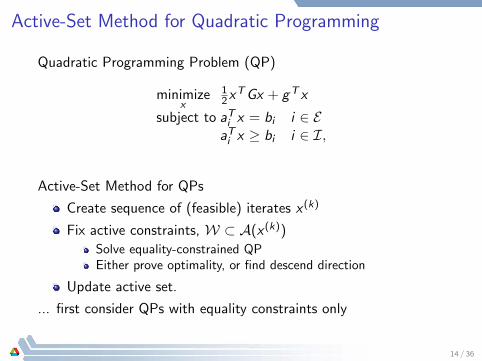
Active-Set Method for Quadratic Programming
Quadratic Programming Problem (QP)
minimizex
12x
TGx + gT x
subject to aTi x = bi i ∈ EaTi x ≥ bi i ∈ I,
Active-Set Method for QPs
Create sequence of (feasible) iterates x (k)
Fix active constraints, W ⊂ A(x (k))
Solve equality-constrained QPEither prove optimality, or find descend direction
Update active set.
... first consider QPs with equality constraints only
14 / 36

Equality-Constrained QPs
Wlog assume solution, x∗, exists (other cases easily detected)
minimizex
12x
TGx + gT x
subject to AT x = b,
where
Columns of matrix A ∈ Rn×m are ai for i ∈ EAssume m ≤ n and A has full rank⇒ which implies that unique multipliers exist
QPs have meaningful solutions even for equality-constraints
If G � 0 positive semi-definite ⇒ x∗ global solution
If G � 0 positive definite ⇒ x∗ is unique
15 / 36

Equality-Constrained QPs
minimizex
12x
TGx + gT x
subject to AT x = b,
A full rank ⇒ partition x and A:
x =
(x1x2
)A =
[A1
A2
],
where x1 ∈ Rm, A1 ∈ Rm×m nonsingular
Then AT x = b ⇔ AT1 x1 + AT
2 x2 = b
A full rank ⇒ A−T1 exists ... eliminate x1:
x1 = A−T1
(b − AT
2 x2)
16 / 36

Equality-Constrained QPs
minimizex
12x
TGx + gT x subject to AT x = b
Partition: x = (x1, x2), similarly for A etc: A−11 exists
In practice, factorize A1 ... check rank!
Check whether Ax = b inconsistent ⇒ QP no solution
Partitioning Hessian, G and gradient g
g =
(g1g2
)G =
[G11 G12
G21 G22
],
⇒ eliminate x1 = A−T1
(b − AT
2 x2), get reduced unconstrained QP:
minimizex2
12x
T2 G̃ x2 + g̃T x2,
For expressions for G̃ and g̃ , see Exercises!
17 / 36
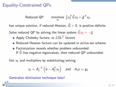
Equality-Constrained QPs
Reduced QP minimizex2
12x
T2 G̃ x2 + g̃T x2,
has unique solution, if reduced Hessian, G̃ � 0, is positive definite
Solve reduced QP by solving the linear system G̃ x2 = −g̃Apply Cholesky factors, or LDLT factors
Reduced Hessian factors can be updated in active-set scheme
Factorization reveals whether problem unbounded:If G̃ has negative eigenvalues, then reduced QP unbounded.
Get x1 and multipliers by substituting/solving
x1 = A−T1
(b − AT
2 x2)
and A1y = g1
Generalize elimination technique later!
18 / 36
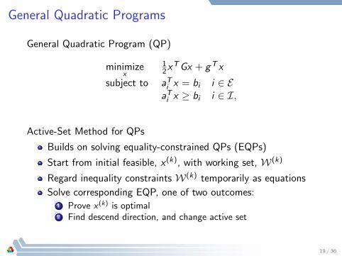
General Quadratic Programs
General Quadratic Program (QP)
minimizex
12x
TGx + gT x
subject to aTi x = bi i ∈ EaTi x ≥ bi i ∈ I,
Active-Set Method for QPs
Builds on solving equality-constrained QPs (EQPs)
Start from initial feasible, x (k), with working set, W(k)
Regard inequality constraints W(k) temporarily as equations
Solve corresponding EQP, one of two outcomes:1 Prove x (k) is optimal2 Find descend direction, and change active set
19 / 36

General Quadratic ProgramsGeneral Quadratic Program (QP)
minimizex
12x
TGx + gT x
subject to aTi x = bi i ∈ EaTi x ≥ bi i ∈ I,
Can have 0 to n active constraints in, W(k): EQP(W(k)):
minimizex
12x
TGx + gT x
subject to aTi x = bi i ∈ W(k),
... solve with any method available for EQPs
Two Key Questions
1 When is solution of EQP(W(k)) optimal for general QP?
2 If EQP(W(k)) not optimal, where’s a descend direction?
20 / 36

Active-Set General QPs
Let solution EQP(W(k)) by x̂ (k)
minimizex
12x
TGx + gT x
subject to aTi x = bi i ∈ W(k),
Solution of EQP(W(k)) is optimal for general QP, iff
If x̂ (k) satisfies inactive inequality constraints:
aTi x̂(k) ≥ bi i ∈ I feasibility test
Multipliers have “right” sign:
y(k)i ≥ 0, ∀i ∈ I ∩W(k) optimality test
21 / 36

Active-Set General QPs
Let solution EQP(W(k)) by x̂ (k)
minimizex
12x
TGx + gT x
subject to aTi x = bi i ∈ W(k),
If solution of EQP(W(k)) is not optimal for general QP, then either
∃q : yq < 0, e.g. yq := min{yi : i ∈ I ∩W(k)}Can move away from constraint q, reducing objectiveGet search direction, s, by solving new EQP forW(k+1) :=W(k) − {q}.
or ...
Inactive constraint becomes feasible ... ratio test
22 / 36

Active-Set Method for Quadratic ProgrammingGiven initial feasible, x (0), and working set, W(0), set k = 0.repeat
if x (k) does not solve the EQP for W(k) thenSolve the EQP(W(k)), get x̂ and set s(k) := x̂ − x (k)
Ratio Test: α = mini∈I:i 6∈W(k),aTi sq<0
{1, bi − aTi x
(k)/(−aTi sq)}
if α < 1 thenUpdate W: Add p (min above) to W(k+1) =W(k) ∪ {p}
Set x (k+1) = x (k) + αs(k) and k = k + 1else
Optimality Test: Find yq := min{yi : i ∈ W(k) ∩ I
}if yq ≥ 0 then x (k) optimal solution ;else
Update W: Remove q from W(k+1) =W(k) − {q}end
end
until x (k) is optimal or QP unbounded ;
23 / 36

Active-Set Method for Quadratic Programming
������������
���������
���������
Iterates are solutions to EQPs, or ratio test.
24 / 36

Active-Set Method for Quadratic Programming
Can implement algorithm in stable/efficient way
Update LU factors of A1
Update LDLT factors of reduced Hessian... can include term for one negative eigenvalue
Get initial feasible point using LP phase I approach
Algorithm is primal active-set method (iterates remain feasible)
Dual active-set method can be derived
Maintains dual feasibility, i.e. multipliers satisfy y(k)i ≥ 0
Move toward primal feasibility
Equivalent to applying primal active-set method to dual QP⇒ requires G−1 to exist!
Fast re-optimization ... good for MIQP solvers
25 / 36

Outline
1 Introduction to Quadratic ProgrammingApplications of QP in Portfolio SelectionApplications of QP in Machine Learning
2 Active-Set Method for Quadratic ProgrammingEquality-Constrained QPsGeneral Quadratic Programs
3 Methods for Solving EQPsGeneralized Elimination for EQPsLagrangian Methods for EQPs
26 / 36

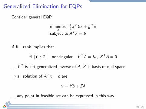
Generalized Elimination for EQPs
Consider general EQP
minimizex
12x
TGx + gT x
subject to AT x = b
Assumption
Assume A ∈ Rn×m, with m ≤ n has full rank
If n = m, then solution of EQP is x = A−1b
Interested in case m < n
A full rank implies that
∃ [Y : Z ] nonsingular Y TA = Im, ZTA = 0
... Y T is left generalized inverse of A, Z is basis of null-space
27 / 36
Generalized Elimination for EQPs
Consider general EQP
minimizex
12x
TGx + gT x
subject to AT x = b
A full rank implies that
∃ [Y : Z ] nonsingular Y TA = Im, ZTA = 0
... Y T is left generalized inverse of A, Z is basis of null-space
⇒ all solution of AT x = b are
x = Yb + Zδ
... any point in feasible set can be expressed in this way.
28 / 36

Generalized Elimination for EQPsConsider general EQP
minimizex
12x
TGx + gT x
subject to AT x = b
⇒ all solution of AT x = b are
x = Yb + Zδ
Use equation to “eliminate” x , get reduced QP:
minimizeδ
12δ
T(ZTGZ
)δ + (g + GYb)T Zδ
If reduced Hessian ZTGZ � 0 pos. def., then unique solution:
∇δ = 0 ⇔(ZTGZ
)δ = −ZT (g + GYb)
29 / 36

Generalized Elimination for EQPs
Consider general EQP
minimizex
12x
TGx + gT x
subject to AT x = b
Once we have δ∗, get
x∗ = Yb + Zδ∗
Find multipliers from
Gx∗ + g = Ay∗ ⇔ y∗ = Y T (Gx∗ + g)
because Y TA = Im, left generalized inverse
30 / 36
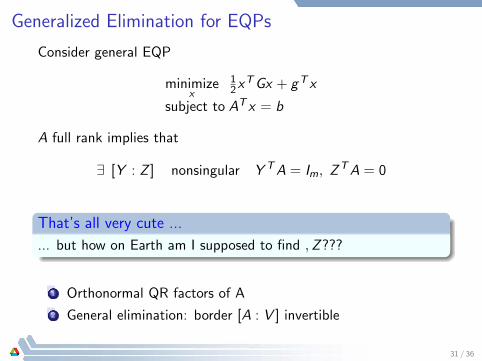
Generalized Elimination for EQPs
Consider general EQP
minimizex
12x
TGx + gT x
subject to AT x = b
A full rank implies that
∃ [Y : Z ] nonsingular Y TA = Im, ZTA = 0
That’s all very cute ...
... but how on Earth am I supposed to find ,Z???
1 Orthonormal QR factors of A
2 General elimination: border [A : V ] invertible
31 / 36
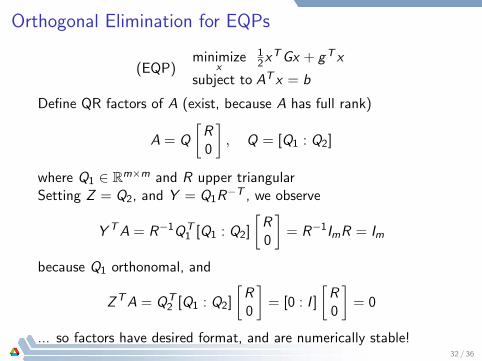
Orthogonal Elimination for EQPs
(EQP)minimize
x
12x
TGx + gT x
subject to AT x = b
Define QR factors of A (exist, because A has full rank)
A = Q
[R0
], Q = [Q1 : Q2]
where Q1 ∈ Rm×m and R upper triangularSetting Z = Q2, and Y = Q1R
−T , we observe
Y TA = R−1QT1 [Q1 : Q2]
[R0
]= R−1ImR = Im
because Q1 orthonomal, and
ZTA = QT2 [Q1 : Q2]
[R0
]= [0 : I ]
[R0
]= 0
... so factors have desired format, and are numerically stable!32 / 36
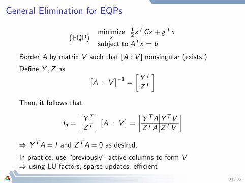
General Elimination for EQPs
(EQP)minimize
x
12x
TGx + gT x
subject to AT x = b
Border A by matrix V such that [A : V ] nonsingular (exists!)
Define Y ,Z as [A : V
]−1=
[Y T
ZT
]Then, it follows that
In =
[Y T
ZT
] [A : V
]=
[Y TA Y TV
ZTA ZTV
]⇒ Y TA = I and ZTA = 0 as desired.
In practice, use “previously” active columns to form V⇒ using LU factors, sparse updates, efficient
33 / 36

General Elimination for EQPs
(EQP)minimize
x
12x
TGx + gT x
subject to AT x = b
Define Y ,Z as [A : V
]−1=
[Y T
ZT
]Border A with special matrix V ... to get first approach[
A1 0
A2 I
]−1
=
[A−11 0
−A2A−11 I
]=
[Y T
ZT
]Then x = Yb + Zδ becomes
x =
[A−T1
0
]b +
[−A−T
1 A−T2
I
]δ
... and δ = x2 ... from our original partition method!34 / 36

Lagrangian Method for EQPs
(EQP)minimize
x
12x
TGx + gT x
subject to AT x = b
Lagrangian: L(x , y) = 12x
TGx + gT x − yT(AT x − b
)First-order optimality gives: ∇xL = 0 and ∇yL = 0:[
G −A−AT 0
](xy
)= −
(gb
)... symmetric system, use factorization that reveals inertia
35 / 36

Summary and Teaching Points
Quadratic Programs
Many applications in finance, data analysis
Building block for algorithms for nonlinear optimization
Active-Set Method for QPs
Generalizes active-set methods for LPs
Moves from EQP to another ... exploring active sets
Method of choice for MIQPs (next week)
������������
���������
���������
36 / 36