CONSTRAINED OPTIMIZATION 2: SEQUENTIAL QUADRATIC ...apmonitor.com/me575/uploads/Main/chap8_constrained_opt_sqp_ip_grg_v2.pdf · linear constraints is known as a quadratic programming

Chapter 8: Constrained Optimization 2

1

CHAPTER 8 CONSTRAINED OPTIMIZATION 2: SEQUENTIAL QUADRATIC

PROGRAMMING, INTERIOR POINT AND GENERALIZED REDUCED GRADIENT METHODS

8.1 Introduction In the previous chapter we examined the necessary and sufficient conditions for a constrained optimum. We did not, however, discuss any algorithms for constrained optimization. That is the purpose of this chapter. The three algorithms we will study are three of the most common. Sequential Quadratic Programming (SQP) is a very popular algorithm because of its fast convergence properties. It is available in MATLAB and is widely used. The Interior Point (IP) algorithm has grown in popularity the past 15 years and recently became the default algorithm in MATLAB. It is particularly useful for solving large-scale problems. The Generalized Reduced Gradient method (GRG) has been shown to be effective on highly nonlinear engineering problems and is the algorithm used in Excel. SQP and IP share a common background. Both of these algorithms apply the Newton-Raphson (NR) technique for solving nonlinear equations to the KKT equations for a modified version of the problem. Thus we will begin with a review of the NR method.

8.2 The Newton-Raphson Method for Solving Nonlinear Equations Before we get to the algorithms, there is some background we need to cover first. This includes reviewing the Newton-Raphson (NR) method for solving sets of nonlinear equations.

8.2.1 One equation with One Unknown The NR method is used to find the solution to sets of nonlinear equations. For example, suppose we wish to find the solution to the equation: 2 xx e+ = We cannot solve for x directly. The NR method solves the equation in an iterative fashion based on results derived from the Taylor expansion. First, the equation is rewritten in the form, 2 0xx e+ - = (8.1) We then provide a starting estimate of the value of x that solves the equation. This point becomes the point of expansion for a Taylor series:


2

fNR ≈ fNR

0 +dfNR

0

dxx − x0( ) (8.2)

where we use the subscript “NR” to distinguish between a function where we are applying the NR method and the objective function of an optimization problem. We would like to drive the value of the function to zero:

0 = fNR

0 +dfNR

0

dxx - x0( ) (8.3)

If we denote Δx0 = x − x0 , and solve for xD in (8.3):

Δx0 =

− fNR0

dfNR0 / dx

(8.4)

We then add xD to 0x to obtain a new guess for the value of x that satisfies the equation, obtain the derivative there, get the new function value, and iterate until the function value or residual, goes to zero. The process is illustrated in Fig. 8.1 for the example given in (8.1) with a starting guess 2.0x = .

1 2 3 x

Second trial, x = 1.469

First trial, x = 2

dy /dx4

2

y 0

- 2

- 4 Fig. 8.1 Newton-Raphson method on (8.1) Numerical results are:

k x f(x) df/dx 1 2 –3.389056 –6.389056 2 1.469553 –0.877738 –3.347291 3 1.20732948 –0.13721157 –2.34454106 4 1.14880563 –0.00561748 –2.15442311 5 1.146198212 –0.000010714 –2.146208926 6 1.1461932206 –0.00000000004 –2.1461932254


3

For simple roots, NR has second order convergence. This means that the number of significant figures in the solution roughly doubles at each iteration. We can see this in the above table where the value of x at iteration 2 has one significant figure (1); at iteration 3 it has one (1); at iteration 4 it has three (1.14); at iteration 5 it has six (1.14619), and so on. We also see that the error in the residual, as indicated by the number of zeros after the decimal point, also decreases in this fashion, i.e., the number of zeros roughly doubles at each iteration.

8.2.2 Multiple Equations with Multiple Unknowns The NR method is easily extended to solve n equation in n unknowns. Writing the Taylor series for the equations in vector form:

0 = f1NR0 + ∇f1NR

0( )TΔx

0 = f2 NR0 + ∇f2 NR

0( )TΔx

… …

0 = fnNR0 + ∇fnNR

0( )TΔx

We can rewrite these relationships as:

∇f1NR0( )

T

∇f2 NR0( )

T

!

∇fnNR0( )

T

⎡

⎣

⎢⎢⎢⎢⎢⎢⎢

⎤

⎦

⎥⎥⎥⎥⎥⎥⎥

Δx =

− f1NR0

− f2 NR0

!− fnNR

0

⎡

⎣

⎢⎢⎢⎢⎢

⎤

⎦

⎥⎥⎥⎥⎥

(8.5)

For 2 X 2 System,

∂ f1NR

∂x1

∂ f1NR

∂x2

∂ f2 NR

∂x1

∂ f2 NR

∂x2

⎡

⎣

⎢⎢⎢⎢⎢

⎤

⎦

⎥⎥⎥⎥⎥

Δx1

Δx2

⎡

⎣

⎢⎢

⎤

⎦

⎥⎥=

− f1NR

− f2 NR

⎡

⎣

⎢⎢

⎤

⎦

⎥⎥ (8.6)

In (8.5) we will denote the vector of residuals at the starting point as fNR

0 . We will denote the matrix of coefficients as G. Equation (8.5) can then be written, GΔx0 = −fNR

0 (8.7) The solution is obviously


4

Δx0 = − G-1( )fNR

0 (8.8)

8.2.3 Using the NR method to Solve the Necessary Conditions In this section we will make a very important connection—we will apply NR to solve the necessary conditions. Consider for example, a very simple case—an unconstrained problem in two variables with objective function, f. We know the necessary conditions are,

1

2

0

0

fxfx

¶=

¶¶

=¶

(8.9)

Now suppose we wish to solve these equations using NR, that is we wish to find the value x* that drives the partial derivatives to zero. In terms of notation and discussion this gets a little tricky because the NR method involves taking derivatives of the equations to be solved, and the equations we wish to solve are composed of derivatives. So when we substitute (8.9) into the NR method, we end up with second derivatives.

For example, if we set f1NR =

∂ f∂x1

and f2 NR =∂ f∂x2

, then we can write (8.6) as,

∂∂x1

∂ f∂x1

⎛

⎝⎜

⎞

⎠⎟

∂∂x2

∂ f∂x1

⎛

⎝⎜

⎞

⎠⎟

∂∂x1

∂ f∂x2

⎛

⎝⎜

⎞

⎠⎟

∂∂x2

∂ f∂x2

⎛

⎝⎜

⎞

⎠⎟

⎡

⎣

⎢⎢⎢⎢⎢

⎤

⎦

⎥⎥⎥⎥⎥

Δx1

Δx2

⎡

⎣

⎢⎢

⎤

⎦

⎥⎥=

−∂ f∂x1

⎛

⎝⎜

⎞

⎠⎟

−∂ f∂x2

⎛

⎝⎜

⎞

⎠⎟

⎡

⎣

⎢⎢⎢⎢⎢

⎤

⎦

⎥⎥⎥⎥⎥

(8.10)

or,

2 2

21 2 1 112 2

22

21 2 2

f f fx x x xx

x ff fxx x x

é ù¶ ¶ ¶é ù-ê ú ê ú¶ ¶ ¶ ¶Dé ùê ú ê ú=ê úê ú D ¶ê ú¶ ¶ ë û -ê ú ê ú¶¶ ¶ ¶ ë ûë û

(8.11)

which should be familiar from Chapter 3, because (8.11) can be written in vector form as, fD = -ÑH x (8.12) and the solution is, ( )1 f-D = - Ñx H (8.13)


5

We recognize (8.13) as Newton’s method for solving for an unconstrained optimum. Thus we have the important result that Newton’s method is the same as applying NR on the necessary conditions for an unconstrained problem. From the properties of the NR method, we know that if Newton’s method converges (and recall that it doesn’t always converge), it will do so with second order convergence. Both SQP and IP methods extend these ideas to constrained problems.

8.3 The Sequential Quadratic Programming (SQP) Algorithm

8.3.1 Introduction and Problem Definition The SQP algorithm was developed in the early 1980’s primarily by M. J. D. Powell, a mathematician at Cambridge University [23, 24]. SQP works by solving for where the KKT equations are satisfied. SQP is a very efficient algorithm in terms of the number of function calls needed to get to the optimum. It converges to the optimum by simultaneously improving the objective and tightening feasibility of the constraints. Only the optimal design is guaranteed to be feasible; intermediate designs may be infeasible. It requires that we have some means of estimating the active constraints at each step of the algorithm. We will start with a problem which only has equality constraints. We recall that when we only have equality constraints, we do not have to worry about complementary slackness, which makes thing simpler. So the problem we will focus on at this point is, Min f (x) (8.14) s.t. gi(x) = 0 i−1,...,m (8.15)

8.3.2 The SQP Approximation As we have previously mentioned in Chapter 7, a problem with a quadratic objective and linear constraints is known as a quadratic programming problem. These problems have a special name because the KKT equations are linear (except for complementary slackness) and are easily solved. We will make a quadratic programming approximation at the point x k to the problem (8.14)-(8.15) given by,

fa = f k + ∇f k( )

TΔx+ 1

2ΔxT∇x

2LkΔx (8.16)

gi,a = gi

k + ∇gik( )

TΔx = 0 i =1,…,m (8.17)

where the subscript a indicates the approximation. Close examination of (8.16) shows something unexpected. Instead of 2 fÑ as we would normally have if we were doing a Taylor approximation of the objective, we have 2

xLÑ , the Hessian of the Lagrangian function with respect to x. Why is this the case? It is directly tied to applying NR on the KKT, as we will presently show. For now we will just accept that the objective uses the Hessian of the Lagrangian instead of the Hessian of the objective.


6

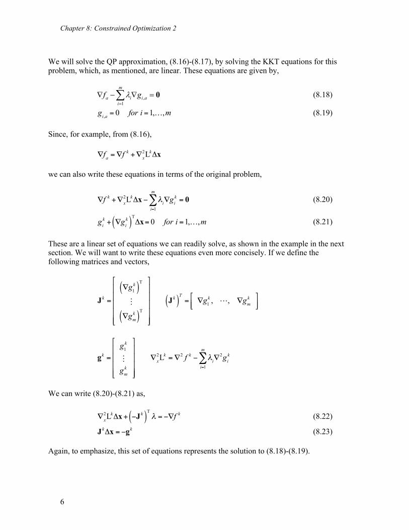
We will solve the QP approximation, (8.16)-(8.17), by solving the KKT equations for this problem, which, as mentioned, are linear. These equations are given by,

,1

m

a i i ai

f gl=

Ñ - Ñ =å 0 (8.18)

gi,a = 0 for i =1,…,m (8.19)

Since, for example, from (8.16), ∇fa =∇f k +∇x

2LkΔx we can also write these equations in terms of the original problem,

∇f k +∇x

2LkΔx − λi∇gik = 0

i=1

m

∑ (8.20)

gi

k + ∇gik( )

TΔx= 0 for i =1,…,m (8.21)

These are a linear set of equations we can readily solve, as shown in the example in the next section. We will want to write these equations even more concisely. If we define the following matrices and vectors,

J k =

∇g1k( )

T

!

∇gmk( )

T

⎡

⎣

⎢⎢⎢⎢⎢

⎤

⎦

⎥⎥⎥⎥⎥

J k( )T= ∇g1

k , ", ∇gmk⎡

⎣⎢⎤⎦⎥

gk =

g1k

!gm

k

⎡

⎣

⎢⎢⎢⎢

⎤

⎦

⎥⎥⎥⎥

∇x2Lk =∇2 f k − λi

i=1

m

∑ ∇2gik

We can write (8.20)-(8.21) as,

∇x

2LkΔx+ −J k( )Tλ = −∇f k (8.22)

JkΔx = −gk (8.23)

Again, to emphasize, this set of equations represents the solution to (8.18)-(8.19).


7

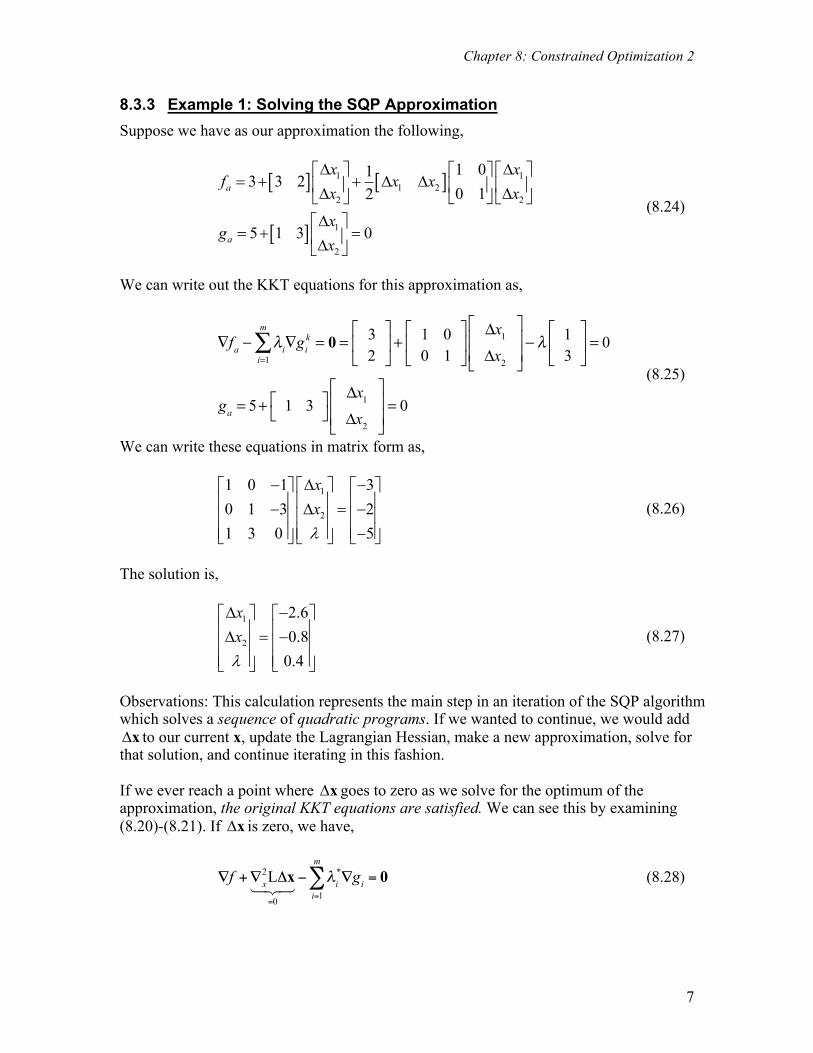
8.3.3 Example 1: Solving the SQP Approximation Suppose we have as our approximation the following,

[ ] [ ]

[ ]

1 11 2

2 2

1

2

1 013 3 20 12

5 1 3 0

a

a

x xf x x

x x

xg

x

D Dé ù é ùé ù= + + D Dê ú ê úê úD Dë ûë û ë û

Dé ù= + =ê úDë û

(8.24)

We can write out the KKT equations for this approximation as,

∇fa − λi∇gik = 0

i=1

m

∑ = 32

⎡

⎣⎢

⎤

⎦⎥ +

1 00 1

⎡

⎣⎢

⎤

⎦⎥

Δx1

Δx2

⎡

⎣⎢⎢

⎤

⎦⎥⎥− λ 1

3⎡

⎣⎢

⎤

⎦⎥ = 0

ga = 5+ 1 3⎡⎣

⎤⎦

Δx1

Δx2

⎡

⎣⎢⎢

⎤

⎦⎥⎥= 0

(8.25)

We can write these equations in matrix form as,

1

2

1 0 1 30 1 3 21 3 0 5

xxl

- D -é ù é ù é ùê ú ê ú ê ú- D = -ê ú ê ú ê úê ú ê ú ê ú-ë û ë û ë û

(8.26)

The solution is,

1

2

2.60.80.4

xxl

D -é ù é ùê ú ê úD = -ê ú ê úê ú ê úë û ë û

(8.27)

Observations: This calculation represents the main step in an iteration of the SQP algorithm which solves a sequence of quadratic programs. If we wanted to continue, we would add Dx to our current x, update the Lagrangian Hessian, make a new approximation, solve for that solution, and continue iterating in this fashion. If we ever reach a point where Dx goes to zero as we solve for the optimum of the approximation, the original KKT equations are satisfied. We can see this by examining (8.20)-(8.21). If Dx is zero, we have,

∇f +∇x2LΔx=0

!"#− λi

*∇gi = 0i=1

m

∑ (8.28)


8

gi + ∇gi( )TΔx

=0! "# $#

= 0 for i =1,…,m (8.29)

which then match (8.18)-(8.19).

8.3.4 NR on the KKT Equations for Problems with Equality Constraints In this section we wish to look at applying the NR method to the original KKT equations. The KKT equations for a problem with equality constraints only are,

1

m

i ii

f gl=

Ñ - Ñ =å 0 (8.30)

gi = 0 i =1,…,m (8.31) Now suppose we wish to solve these equations using the NR method. The coefficient matrix for NR will be composed of the derivatives of (8.30)-(8.31). For example, the first row of the coefficient matrix would be,

∇x f1NR( )T∇λ f1NR( )T⎡

⎣⎢

⎤

⎦⎥

ΔxΔλ

⎡

⎣⎢

⎤

⎦⎥= −

f1NR

f2 NR

⎡

⎣

⎢⎢

⎤

⎦

⎥⎥ (8.32)

where function f1NR given by,

f1NR =

∂ f∂x1

− λi

∂gi

∂x1i=1

m

∑ (8.33)

If we substitute (8.33) into (8.32), the first row becomes,

∂2 f∂x1

2 − λi

∂2 gi

∂x12

i=1

m

∑⎡

⎣⎢

⎤

⎦⎥, ∂2 f

∂x2 ∂x1

− λi

∂2 gi

∂x2 ∂x1i=1

m

∑⎡

⎣⎢

⎤

⎦⎥,…, ∂2 f

∂xn ∂x1

− λi

∂2 gi

∂xn ∂x1i=1

m

∑⎡

⎣⎢

⎤

⎦⎥, −

∂g1

∂x1

⎡

⎣⎢

⎤

⎦⎥, −

∂g2

∂x1

⎡

⎣⎢

⎤

⎦⎥,…, −

∂gm

∂x1

⎡

⎣⎢

⎤

⎦⎥

Recalling,

2 2 2

1

m

x i ii

L f gl=

Ñ =Ñ - Ñå

And using the matrices,

J k =

∇g1k( )

T

!

∇gmk( )

T

⎡

⎣

⎢⎢⎢⎢⎢

⎤

⎦

⎥⎥⎥⎥⎥

J k( )T= ∇g1

k , ", ∇gmk⎡

⎣⎢⎤⎦⎥


9

gk =

g1k

!gm

k

⎡

⎣

⎢⎢⎢⎢

⎤

⎦

⎥⎥⎥⎥

∇x2Lk =∇2 f k − λi

i=1

m

∑ ∇2gik

we can write the NR equations in matrix form as,

∇x2Lk −J k( )

T

J k 0

⎡

⎣

⎢⎢

⎤

⎦

⎥⎥

x −x k

λ −λ k

⎡

⎣⎢⎢

⎤

⎦⎥⎥=

−∇f k + J k( )Tλ k

−(gk )

⎡

⎣

⎢⎢⎢

⎤

⎦

⎥⎥⎥ (8.34)

If we do the matrix multiplications we have

∇x

2LkΔx+ −J k( )T

(λ −λ k ) = −∇f k + J k( )Tλ k (8.35)

J kΔx = − gk( )

and collecting terms,

∇x

2LkΔx+ −J k( )Tλ = −∇f k (8.36)

J kΔx = − gk( )

which equations are the same as (8.22)-(8.23)). Thus we see that solving for the optimum of the QP approximation is the same as doing a NR iteration on the KKT equations. This is the reason we use the Hessian of the Lagrangian function rather than the Hessian of the objective in the approximation.

8.3.5 SQP: Inequality and Equality Constraints In the previous section we considered equality constraints only. We need to extend these results to the general case. We will state this problem as Min ( )f x

s.t. gi x( ) ≥ 0 i =1,…,k (8.37)

gi x( ) = 0 i = k +1,…,m

The quadratic approximation at point xk is:

Min fa = f k + ∇f k( )

TΔx+ 1

2Δx( )T

∇x2LkΔx

s.t. , :i ag gi

k + ∇gik( )

TΔx ≥ 0 i =1,2,...,k (8.38)


10

gi

k + ∇gik( )

TΔx = 0 i = k +1,...,m

Notice that the approximations are a function only of ∆x. All gradients and the Lagrangian hessian in (7.40) are evaluated at the point of expansion and so represent known quantities. In the article where Powell [24] describes this algorithm he makes a significant statement at this point. Quoting, “The extension of the Newton iteration to take account of inequality constraints on the variables arises from the fact that the value of Dx that solves (8.36) can also be found by solving a quadratic programming problem. Specifically, Dx is the value that makes the quadratic function in (8.38) stationary.” Further, the value of l for the KKT conditions is equal to the vector of Lagrange multipliers of the quadratic programming problem. Thus solving the quadratic objective and linear constraints in (8.38) is the same as solving the NR iteration on the original KKT equations. The main difficulty in extending SQP to the general problem has to do the with the complementary slackness condition. This equation is nonlinear, and so makes the QP problem nonlinear. We recall that complementary slackness basically enforces that either a constraint is binding or the associated Lagrange multiplier is zero. Thus we can incorporate this condition if we can develop a method to determine which inequality constraints are binding at the optimum. An example of such a solution technique is given by Goldfarb and Idnani [25]. This algorithm starts out by solving for the unconstrained optimum to the problem and evaluating which constraints are violated. It then moves to add in these constraints until it is at the optimum. Thus it tends to drive to the optimum from infeasible space. There are other important details to develop a realistic, efficient SQP algorithm. For example, the QP approximation involves the Lagrangian hessian matrix, which involves second derivatives. As you might expect, we don't evaluate the Hessian directly but approximate it using a quasi-Newton update, such as the BFGS update. Recall that updates use differences in x and differences in gradients to estimate second derivatives. To estimate 2LxÑ we will need to use differences in the gradient of the Lagrangian function,

1

Lm

x i ii

f gl=

Ñ =Ñ - Ñå

Note that to evaluate this gradient we need values for li. We will get these from our solution to the QP problem. Since our update stays positive definite, we don’t have to worry about the method diverging like Newton’s method does for unconstrained problems.

8.3.6 Comments on the SQP Algorithm The SQP algorithm has the following characteristics,

• The algorithm is usually very fast.


11

• Because it does not rely on a traditional line search, it is often more accurate in identifying an optimum.

• The efficiency of the algorithm is partly because it does not enforce feasibility of the constraints at each step. Rather it gradually enforces feasibility as part of the KKT conditions. It is only guaranteed to be feasible at the optimum.

Relative to engineering problems, there are some drawbacks:

• Because it can go infeasible during optimization—sometimes by relatively large amounts—it can crash engineering models.

• It is more sensitive to numerical noise and/or error in derivatives than GRG. • If we terminate the optimization process before the optimum is reached, SQP does not

guarantee that we will have in-hand a better design than we started with.

8.3.7 Summary of Steps for SQP Algorithm 1. Make a QP approximation to the original problem. For the first iteration, use a

Lagrangian Hessian equal to the identity matrix.

2. Solve for the optimum to the QP problem. As part of this solution, values for the Lagrange multipliers are obtained.

3. Execute a simple line search by first stepping to the optimum of the QP problem. So the

initial step is ∆x, and new old= +Dx x x. See if at this point a penalty function, composed of the values of the objective and violated constraints, is reduced. If not, cut back the step size until the penalty function is reduced. The penalty function is given

by1

vio

i ii

P f gl=

= +å where the summation is done over the set of violated constraints, and

the absolute values of the constraints are taken. The Lagrange multipliers act as scaling or weighting factors between the objective and violated constraints.

4. Evaluate the Lagrangian gradient at the new point. Calculate the difference in x and in the Lagrangian gradient, g. Update the Lagrangian Hessian using the BFGS update.

5. Return to Step 1 until ∆x is sufficiently small. When ∆x approaches zero, the KKT

conditions for the original problem are satisfied.

8.3.8 Example of SQP Algorithm Find the optimum to the problem, Min ( ) 4 2 2 2

1 2 1 2 1 12 2 5f x x x x x x= - + + - +x

s.t. ( ) ( )21 20.25 0.75 0g x x= - + + ³x starting from the point [ ]-1,4 . A contour plot of the problem is shown in Fig. 8.2. This is similar to Rosenbrock’s function with a constraint. The problem is interesting for several reasons: the objective is quite eccentric at the optimum, the algorithm starts at a point where


12

the search direction is pointing away from the optimum, and the constraint boundary at the starting point has a slope opposite to that at the optimum.

Fig. 8.2. Contour plot of example problem for SQP algorithm.

Iteration 1 We calculate the gradients, etc. at the beginning point. The Lagrangian Hessian is initialized to the identity matrix.

At ( ) [ ] ( ) [ ]T0 0 0 2 0 1 0-1,4 , 17, 8,6 , L

0 1T

f f é ù= = Ñ = Ñ = ê ú

ë ûx

( ) [ ]0 02.4375, 1.5, 0.75T

g g= Ñ = Based on these values, we create the first approximation,

[ ] [ ]1 11 2

2 2

1 0117.0 8 60 12a

x xf x x

x xD Dé ù é ùé ù

= + + D Dê ú ê úê úD Dë ûë û ë û

[ ] 1

2

2.4375 1.5 0.75 0a

xg

xDé ù

= + ³ê úDë û

We will assume the constraint is binding. Then the KKT conditions for the optimum of the approximation are given by the following equations: 0a af glÑ - Ñ =


13

0ag = These equations can be written as, ( )18 1.5 0x l+D - =

( )26 0.75 0x l+D - = 1 22.4375 1.5 0.75 0x x+ D + D = The solution to this set of equations is 1 20.5, 2.25, 5.00x x lD = - D = - =

The proposed step is, 1 0 1 0.5 1.5

4 2.25 1.75- - -é ù é ù é ù

= +D = + =ê ú ê ú ê ú-ë û ë û ë ûx x x

Before we accept this step, however, we need to check the penalty function,

1

vio

i ii

P f gl=

= +å

to make sure it decreased with the step. At the starting point, the constraint is satisfied, so the penalty function is just the value of the objective, 17P = . At the proposed point the objective value is 10.5f = and the constraint is slightly violated with 0.25g = - . The penalty function is therefore, 10.5 5.0* 0.25 11.75P = + - = . Since this is less than 17, we accept the full step. Contours of the first approximation and the path of the first step are shown in Fig. 8.3.

Fig. 8.3 The first SQP approximation and step.


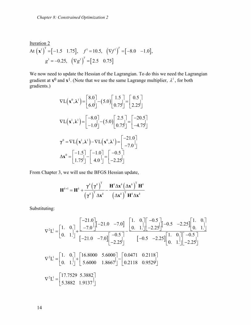
14

Iteration 2 At ( ) [ ] ( ) [ ]T1 1 11.5 1.75 , 10.5, 8.0 1.0 ,

Tf f= - = Ñ = - -x

( ) [ ]1 10.25, 2.5 0.75T

g g= - Ñ = We now need to update the Hessian of the Lagrangian. To do this we need the Lagrangian gradient at x0 and x1. (Note that we use the same Lagrange multiplier, 1l , for both gradients.)

( ) ( )0 1 8.0 1.5 0.5L , 5.0

6.0 0.75 2.25é ù é ù é ù

Ñ = - =ê ú ê ú ê úë û ë û ë û

x λ

( ) ( )1 1 8.0 2.5 20.5L , 5.0

1.0 0.75 4.75- -é ù é ù é ù

Ñ = - =ê ú ê ú ê ú- -ë û ë û ë ûx λ

( ) ( )0 1 1 0 1 21.0L , L ,

7.0-é ù

=Ñ -Ñ = ê ú-ë ûγ x λ x λ

0 1.5 1.0 0.51.75 4.0 2.25- - -é ù é ù é ù

D = - =ê ú ê ú ê ú-ë û ë û ë ûx

From Chapter 3, we will use the BFGS Hessian update,

( )

( )( )

( )

T T

1T T

k k k k k kk k

k k k k k

+D D

= + -D D D

γ γ H x x HH H

γ x x H x

Substituting:

[ ]

[ ]

[ ]

[ ]2 1

21.0 1. 0. 0.5 1. 0.21.0 7.0 0.5 2.25

1. 0. 7.0 0. 1. 2.25 0. 1.L

0.5 1. 0. 0.50. 1.21.0 7.0 0.5 2.25

2.25 0. 1. 2.25

- -é ù é ù é ù é ù- - - -ê ú ê ú ê ú ê ú- -é ù ë û ë û ë û ë ûÑ = + -ê ú - -é ù é ù é ùë û - - - -ê ú ê ú ê ú- -ë û ë û ë û

2 1 1. 0. 16.8000 5.6000 0.0471 0.2118L

0. 1. 5.6000 1.8667 0.2118 0.9529é ù é ù é ù

Ñ = + -ê ú ê ú ê úë û ë û ë û

2 1 17.7529 5.3882L

5.3882 1.9137é ù

Ñ = ê úë û


15

The second approximation is therefore,

[ ] [ ]1 11 2

2 2

17.753 5.3882110.5 8.0 1.05.3882 1.91372a

x xf x x


= + - - + D Dê ú ê úê úD Dë ûë û ë û

[ ] 1

2

0.25 2.5 0.75 0a

xg

xDé ù

= - + ³ê úDë û

As we did before, we will assume the constraint is binding. The KKT equations are, ( )1 28 17.753 5.3882 2.5 0x x l- + D + D - =

( )1 21 5.3882 1.9137 0.75 0x x l- + D + D - = 1 20.25 2.5 0.75 0x x- + D + D = The solution to this set of equations is 1 21.6145, 5.048, 2.615x x lD = D = - = - . Because l is negative, we need to drop the constraint from the picture. (We can see in Fig. 8.4 below that the constraint is not binding at the optimum.) With the constraint dropped, the solution is, 1 22.007, 5.131, 0.x x lD = D = - = This gives a new x of,

2 1 1.5 2.007 0.507

1.75 5.131 3.381-é ù é ù é ù

= +D = + =ê ú ê ú ê ú- -ë û ë û ë ûx x x

However, when we try to step this far, we find the penalty function has increased from 11.75 to 17.48 (this is the value of the objective only—the violated constraint does not enter in to the penalty function because the Lagrange multiplier is zero). We cut the step back. How much to cut back is somewhat arbitrary. We will make the step 0.5 times the original. The new value of x becomes,

2 1 1.5 2.007 0.49650.5

1.75 5.131 0.8155- -é ù é ù é ù


At which point the penalty function is 7.37. So we accept this step. Contours of the second approximation are shown in Fig. 8.4, along with the step taken.


16

Fig. 8.4 The second approximation and step.

Iteration 3 At ( ) [ ] ( ) [ ]T2 2 20.4965 0.8155 , 7.367, 5.102 2.124 ,

Tf f= - - = Ñ = - -x

( ) [ ]2 20.6724, 0.493 0.75T

g g= - Ñ =

( ) ( )1 2 8.0 2.5 8.0L , 0

1.0 0.75 1.0- -é ù é ù é ù


( ) ( )2 2 5.102 0.493 5.102L , 0

2.124 0.75 2.124- -é ù é ù é ù


( ) ( )1 2 2 1 2 2.898L , L ,

1.124é ù

=Ñ -Ñ = ê ú-ë ûγ x λ x λ

1 0.4965 1.5 1.0040.8155 1.75 2.5655- -é ù é ù é ù

D = - =ê ú ê ú ê ú- -ë û ë û ë ûx

Based on these vectors, the new Lagrangian Hessian is,

2 2 17.7529 5.3882 1.4497 0.5623 5.8551 0.7320L

5.3882 1.9137 0.5623 0.2181 0.7320 0.0915-é ù é ù é ù

Ñ = + -ê ú ê ú ê ú-ë û ë û ë û


17

∇2L2 =

13.3475 4.09394.0939 2.0403⎡

⎣⎢

⎤

⎦⎥

So our next approximation is,

[ ] [ ]1 11 2

2 2

13.3475 4.093917.367 5.102 2.1244.0939 2.04032a

x xf x x



[ ] 1

2

0.6724 0.493 0.75 0a

xg

xDé ù

= - + ³ê úDë û

The KKT equations, assuming the constraint is binding, are, ( )1 25.102 13.3475 4.0939 0.493 0x x l- + D + D - =

( )1 22.124 4.0939 2.0403 0.75 0x x l- + D + D - = 1 20.6724 0.493 0.75 0x x- + D + D = The solution to this set of equations is 1 20.1399, 0.8046, 0.1205x x lD = D = = .

Our new proposed point is, 3 2 0.4965 0.1399 0.3566

0.8155 0.8046 0.0109- -é ù é ù é ù


At this point the penalty function has decreased from 7.37 to 5.85. We accept the full step. A contour plot of the third approximation is shown in Fig. 8.5.

Fig. 8.5 The third approximation and step.


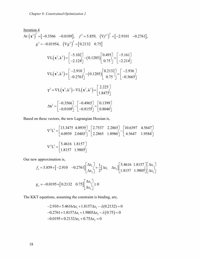
18

Iteration 4 At ( ) [ ] ( ) [ ]3 3 30.3566 0.0109 , 5.859, 2.9101 0.2761 ,

T Tf f= - - = Ñ = - -x

( ) [ ]3 30.01954, 0.2132 0.75T

g g= - Ñ =

( ) ( )2 3 5.102 0.493 5.161L , 0.1205

2.124 0.75 2.214- -é ù é ù é ù


( ) ( )3 3 2.910 0.2132 2.936L , 0.1205

0.2761 0.75 0.3665- -é ù é ù é ù


( ) ( )2 3 3 2 3 2.225L , L ,

1.8475é ù

=Ñ -Ñ = ê úë û

γ x λ x λ

2 0.3566 0.4965 0.13990.0109 0.8155 0.8046- -é ù é ù é ù

D = - =ê ú ê ú ê ú- -ë û ë û ë ûx

Based on these vectors, the new Lagrangian Hessian is,

2 3 13.3475 4.0939 2.7537 2.2865 10.6397 4.5647L

4.0939 2.0403 2.2865 1.8986 4.5647 1.9584é ù é ù é ù

Ñ = + -ê ú ê ú ê úë û ë û ë û

2 3 5.4616 1.8157L

1.8157 1.9805é ù

Ñ = ê úë û

Our new approximation is,

[ ] [ ]1 11 2

2 2

5.4616 1.815715.859 2.910 0.27611.8157 1.98052a

x xf x x



[ ] 1

2

0.0195 0.2132 0.75 0a

xg

xDé ù

= - + ³ê úDë û

The KKT equations, assuming the constraint is binding, are, 1 22.910 5.4616 1.8157 (0.2132) 0x x l- + D + D - = ( )1 20.2761 1.8157 1.9805 0.75 0x x l- + D + D - = 1 20.0195 0.2132 0.75 0x x- + D + D =


19

The solution to this problem is, 1 20.6099, 0.1474, 0.7192x x lD = D = - = . Since l is positive, our assumption about the constraint was correct. Our new proposed point is,

4 3 0.3566 0.6099 0.2533

0.0109 0.1474 0.1583-é ù é ù é ù

= +D = + =ê ú ê ú ê ú- - -ë û ë û ë ûx x x

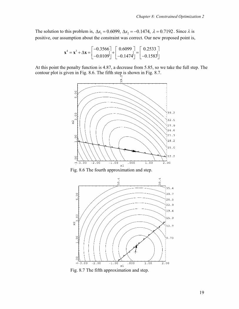
At this point the penalty function is 4.87, a decrease from 5.85, so we take the full step. The contour plot is given in Fig. 8.6. The fifth step is shown in Fig. 8.7.

Fig. 8.6 The fourth approximation and step.

Fig. 8.7 The fifth approximation and step.


20

We would continue in this fashion until Dx goes to zero. We would then know the original KKT equations were satisfied. The solution to this problem occurs at,

x*( )

T= 0.500 0.750⎡⎣⎢

⎤⎦⎥, f * = 4.50

A summary of five steps is overlaid on the original problem in Fig. 8.8.

Fig. 8.8 The path of the SQP algorithm.


21

8.4 The Interior Point (IP) Algorithm

8.4.1 Problem Definition In general, for the primal-dual method given here, there are two approaches to developing the equations for the IP method: putting slack variables into their own vector, and incorporating slack variables as part of the design variables x. Both methods can be found in the literature. We have opted for the former, because the development is somewhat more straightforward. It is also the approach used in MATLAB. The development of the latter is given in a later optional section. For simplicity, we will start with a problem that only has inequality constraints. Min ( )f x (8.39)

s.t. gi x( ) ≥ 0 i =1,…,m (8.40)

We will add in slack variables to turn the inequalities into equalities: Min ( )f x (8.41)

s.t. gi x( )− si = 0 i =1,…,m (8.42)

si ≥ 0 i =1,...,m (8.43) Slack variables are so named because they take up the “slack” between the constraint value and the right hand side. For an inequality constraint to be feasible, si must be ≥ 0. If (8.42) is satisfied and si = 0, then the original inequality is binding. The IP algorithm eliminates the lower bounds on s by incorporating a barrier function as part of the objective:

Min fµ = f x( )−µ ln(si

i=1

m

∑ ) (8.44)

s.t. gi x( )− si = 0 i =1,…,m (8.45)

We note that as si approaches zero (from a positive value, i.e. from feasible space), the negative barrier term goes to infinity. This obviously penalizes the objective and forces the algorithm to keep s positive. The IP algorithm solves a sequence of these problems for a decreasing set of barrier parametersµ . Asµ approaches zero, the barrier becomes steeper and sharper. This is illustrated in Fig. 8.9.


22

0 1 2 3 4 5x

-40

-20

0

20

40

60

80

100

120

140

Fig. 8.9 Barrier function −µ ln(x) for µ =20, 10 and 1.

We can define the Lagrangian function for this problem as,

L(x,s,λ) = f (x)−µ ln(si )−

i=1

m

∑ λi(gi(x)− sii=1

m

∑ ) (8.46)

Taking the gradient of this function with respect to x, s, λ , and setting it equal to zero gives us the KKT conditions for (8.44)–(8.45),

∇x L =∇f (x)− λi∇gi(x)

i=1

m

∑ = 0 (8.47)

∇sL = siλi −µ = 0 i =1,…,m (8.48) ∇λL = −(gi(x)− si ) = 0 i =1,…,m (8.49) If we define e as the vector of 1’s of m dimension and,

S =s1 0!

0 sm

⎛

⎝

⎜⎜⎜⎜

⎞

⎠

⎟⎟⎟⎟

Λ =

λ1 0!

0 λm

⎛

⎝

⎜⎜⎜⎜

⎞

⎠

⎟⎟⎟⎟

we can replace (8.48) above with (8.51) below,


23

∇f (x)− λi∇gi(x)

i=1

m

∑ = 0 (8.50)

SΛe−µe = 0 (8.51) gi(x)− si = 0 i =1,…,m (8.52) It is worth noting that as µ→ 0 , the above equations (along with λ,s ≥ 0 ) represent the KKT conditions for the original problem (8.39)-(8.40). Notice that with µ = 0 , (8.51) (perhaps more easily seen in (8.48)) expresses complementary slackness for the slack variable bounds, i.e. either λi = 0 or si = 0 .

8.4.2 Problem Solution We will use the NR method to solve the set of equations represented by (8.50)-(8.52). The coefficient matrix (see 8.5) will be the first derivatives of these equations. We note that we have n equations from (8.50), m equations from (8.51) and m equations from (8.52). Similarly, these equations are functions of n variables x, m variables l, and m variables s. The coefficient matrix for NR can be represented as,

∇x f1NR( )T∇s f1NR( )T

∇λ f1NR( )T

! ! !

∇x f(n+2m) NR( )T

∇s f(n+2m) NR( )T

∇λ f(n+2m) NR( )T

⎡

⎣

⎢⎢⎢⎢⎢

⎤

⎦

⎥⎥⎥⎥⎥

ΔxΔsΔλ

⎡

⎣

⎢⎢⎢

⎤

⎦

⎥⎥⎥= −

r1r2r3

⎡

⎣

⎢⎢⎢

⎤

⎦

⎥⎥⎥ (8.53)

where f1NR (the first NR equation) is given by,

f1NR =

∂ f∂x1

− λi

∂gi

∂x1i=1

m

∑ (8.54)

and r1, r2 and r3 represent the residuals for (8.50)–(8.52). If we substitute (8.54) into the first row of (8.53), the first row of the coefficient matrix becomes,

∂2 f∂x1

2 − λi

∂2 gi

∂x12

i=1

m

∑⎡

⎣⎢

⎤

⎦⎥,…, ∂2 f

∂xn ∂x1

− λi

∂2 gi

∂xn ∂x1i=1

m

∑⎡

⎣⎢

⎤

⎦⎥

∇x f T! "######## $########

, 0⎡⎣ ⎤⎦,…, 0⎡⎣ ⎤⎦∇s f T

! "# $#, −

∂g1

∂x1

⎡

⎣⎢

⎤

⎦⎥,..., −

∂gm

∂x1

⎡

⎣⎢

⎤

⎦⎥

∇λ f T! "### $###

Recalling,

∇x

2 L =∇2 f − λi∇2gi

i=1

m

∑ (8.55)

and


24

J k =

∇g1k( )

T

!

∇gmk( )

T

⎡

⎣

⎢⎢⎢⎢⎢

⎤

⎦

⎥⎥⎥⎥⎥

J k( )T= ∇g1

k , " ∇gmk⎡

⎣⎢⎤⎦⎥

we can write the NR iteration equations at step k as,

∇x2Lk 0 −J k( )

T

0 Λ k Sk

J k −I 0

⎡

⎣

⎢⎢⎢⎢⎢

⎤

⎦

⎥⎥⎥⎥⎥

Δx k

Δsk

Δλ k

⎡

⎣

⎢⎢⎢⎢

⎤

⎦

⎥⎥⎥⎥

= −

∇f k (x)− λik∇gi

k (x)i=1

m

∑

SkΛ ke−µ ke

gik (x)− si

k

⎡

⎣

⎢⎢⎢⎢⎢⎢⎢

⎤

⎦

⎥⎥⎥⎥⎥⎥⎥

(8.56)

At this point, we could solve this system of equations to obtain Dxk, Dsk, and Dlk. However, for large problems we can gain efficiency by simplifying this expression. If we look at row 2 above, Λ

kΔsk +SkΔλ k = −SkΛ ke+µe (8.57) We would like to solve (8.57) for Dsk. Rearranging terms and pre-multiplying both sides by

Λ k( )

−1 gives,

Δsk = − Λ k( )

−1SkΛe+µΛ−1e−Λ−1SkΔx k (8.58)

For diagonal matrices, the order of matrix multiplication does not matter, so the first term on the right hand side simplifies to give, Δsk = −Ske+µΛ−1e−Λ−1SkΔx k (8.59) Examining the first and second terms on the right hand side, we note that,

−Ske = −s1

k 0!

0 snk

⎛

⎝

⎜⎜⎜⎜

⎞

⎠

⎟⎟⎟⎟

1"1

⎡

⎣

⎢⎢⎢

⎤

⎦

⎥⎥⎥= −sk µ(Λ k )−1e =

µλ1

k 0!

0 µλm

k

⎛

⎝

⎜⎜⎜⎜⎜⎜⎜

⎞

⎠

⎟⎟⎟⎟⎟⎟⎟

1"1

⎡

⎣

⎢⎢⎢

⎤

⎦

⎥⎥⎥= sk

Equation (8.59) becomes,


25

Δsk = −sk + sk − (Λ k )−1SkΔx k

= −(Λ k )−1SkΔx k (8.60)

We define Ω to be, Ω

k = (Λ k )−1Sk (8.61) so that we have, Δsk = −ΩkΔλ k (8.62) We can then write (8.56) as a reduced set of equations:

−∇x2Lk J k( )

T

J k Ωk

⎡

⎣

⎢⎢

⎤

⎦

⎥⎥

Δx k

Δλ k

⎡

⎣⎢⎢

⎤

⎦⎥⎥= −

−∇f (x)+ λi∇gi(x)i=1

m

∑

gi(x)− si

⎡

⎣

⎢⎢⎢⎢

⎤

⎦

⎥⎥⎥⎥

(8.63)

This matrix represents a linear symmetric system of equations (symmetric because the off-diagonal elements are the transpose of one another), of lower dimension than (8.56) and is more efficiently solved. Once we have solved for Δλ k , we can use (8.62) to get Δsk .

8.4.3 The Line Search It is sometimes said, “the devil is in the details.” That is certainly true for the line search for the IP method. Modern algorithms employ a number of line search techniques, including merit functions, trust regions and filter methods [26, 27, 28]. They include techniques to handle non-positive-definite hessians or otherwise poorly conditioned problems, or to regain feasibility. Sometimes a different step length is used for the primal variables (x, s) and the dual variables (l). We will adopt that strategy here as well. We can consider Δx, Δs, Δλ, as the search directions for x, s, and l. We then need to determine the step size (between 0-1) in these directions, x k+1 = x k +α kΔx k (8.64) λ k+1 = λ k +α kΔλ k (8.65) s

k+1 = sk +α kΔsk (8.66) Similar to SQP, a straightforward method is to accept a if it results in a decrease in a merit function that combines the objective with a sum of the violated constraints, i.e.,

P = f k +ν gi

i=1

viol

∑


26

where n is a constant. We will also reduce the step length if necessary to keep a slack variable or a Lagrange multiplier positive.

8.4.4 Example 1: Two Variables, One Constraint We will apply the IP method to the same example given for SQP in Section 8.3.8, namely, Min ( ) 4 2 2 2

1 2 1 2 1 12 2 5f x x x x x x= - + + - +x

s.t. ( ) ( )21 20.25 0.75 0g x x= - + + ³x We reformulate the problem using a slack variable, s1, for the constraint: Min ( ) 4 2 2 2

1 2 1 2 1 12 2 5f x x x x x x= - + + - +x

s.t.

g x( ) = − x1+0.25( )2+0.75x2 − s1 = 0

s1 ≥ 0

We eliminate the lower bound for s1 by adding a barrier term, Min

fµ x( ) = f (x)−µ ln(s1)

s.t. g x( ) = − x1+0.25( )2

+0.75x2 − s1 = 0 At the starting point we have,

x0( )

T= -1,4⎡⎣ ⎤⎦, f 0 =17, ∇f 0( )

T= 8,6⎡⎣ ⎤⎦,

g0 = 2.4375, ∇g0( )T= 1.5, 0.75⎡⎣ ⎤⎦

We will assume we do not have second derivatives available, so we will begin with the

Hessian set to ∇2L0 =

1 00 1

⎡

⎣⎢

⎤

⎦⎥ . J

0 = [1.5, 0.75] . We will also set µ0 = 5 , s1

0 = 2.4375 , λ10 = 2 .

This value of l was picked to approximately satisfy (8.51), i.e. λ0s0 −µ0 = 0 .

If the merit function increases for a proposed step, we will cut the step in half and continue doing so several times.

8.4.4.1 First Iteration Based on the data above, the coefficient matrix (refer back to (8.56)) for the first step is,


27

1 0 0 −1.50 1 0 −0.750 0 2 2.4375

1.5 0.75 −1 0

⎡

⎣

⎢⎢⎢⎢

⎤

⎦

⎥⎥⎥⎥

For the residual vector, we have,

∇f k (x)− λi

k∇gik (x) =

i=1

m

∑ 86

⎡

⎣⎢

⎤

⎦⎥−2 1.5

0.75

⎡

⎣⎢

⎤

⎦⎥= 5

4.5

⎡

⎣⎢

⎤

⎦⎥

SkΛ ke−µ ke = 2.4375⎡⎣ ⎤⎦ 2⎡⎣ ⎤⎦− 5⎡⎣ ⎤⎦= −0.125⎡⎣ ⎤⎦

gi

k (x)− sik = 2.4375⎡⎣ ⎤⎦− 2.4375⎡⎣ ⎤⎦= 0⎡⎣ ⎤⎦

Thus the set of equations for our first step becomes,

1 0 0 −1.50 1 0 −0.750 0 2 2.4375

1.5 0.75 −1 0

⎡

⎣

⎢⎢⎢⎢

⎤

⎦

⎥⎥⎥⎥

Δx0

Δs0

Δλ 0

⎡

⎣

⎢⎢⎢

⎤

⎦

⎥⎥⎥= −

54.5

−0.1250

⎡

⎣

⎢⎢⎢⎢

⎤

⎦

⎥⎥⎥⎥

The solution is ΔxT = [−0.930, −2.465], Δs = −3.244, Δλ = 2.713 Because the full step would make the slack negative, we set the step length for x and s to be 0.748 to keep the slack slightly positive. We accept the full step for l. At this trial point the objective has decreased to 11.78 but the constraint is violated at –0.471. However the merit function has decreased from 17 to 14.00 and we accept the step. Our new point is

xT = [−1.695, 2.157], s = 0.012, λ = 4.713 .

8.4.4.2 Second Iteration

At x1( )

T= [−1.695, 2.157], f 1 =11.78, ∇f 1( )

T= [−10.256 −1.435]

g1 = −0.4714, ∇g1( )

T= [2.891 0.75]

We start this step by updating the Hessian of the Lagrangian. To do so, we evaluate the Lagrangian gradient at x0 and x1 . We then calculate the g and Dx vectors. (As we did for SQP, we use the same Lagrange multiplier, 1l , for both gradients.)

∇L x0 ,λ1( ) = 8.0

6.0

⎡

⎣⎢

⎤

⎦⎥− 4.713( ) 1.5

0.75

⎡

⎣⎢

⎤

⎦⎥= 0.930

2.465

⎡

⎣⎢

⎤

⎦⎥


28

∇L x1,λ1( ) = −10.256

−1.435

⎡

⎣⎢

⎤

⎦⎥− 4.713( ) 2.891

0.75

⎡

⎣⎢

⎤

⎦⎥= −23.881

−4.967

⎡

⎣⎢

⎤

⎦⎥

γ 0 =∇L x1,λ1( )−∇L x0 ,λ1( ) = −24.811

−7.435

⎡

⎣⎢

⎤

⎦⎥

Δx0 = −1.695

2.157

⎡

⎣⎢

⎤

⎦⎥− −1.0

4.0

⎡

⎣⎢

⎤

⎦⎥= −0.695

−1.843

⎡

⎣⎢

⎤

⎦⎥

We use this data to obtain the new estimate of the Lagrangian Hessian using BFGS Hessian update, as we did for SQP (see the SQP example for details). The new Hessian is,

∇2L1 =

20.762 5.6295.629 1.910

⎡

⎣⎢

⎤

⎦⎥

After evaluating the residuals, our next set of equations becomes,

20.762 5.629 0 −2.8915.629 1.910 0 −0.75

0 0 4.713 0.0122.891 0.75 −1 0

⎡

⎣

⎢⎢⎢⎢

⎤

⎦

⎥⎥⎥⎥

Δx1

Δs1

Δλ1

⎡

⎣

⎢⎢⎢

⎤

⎦

⎥⎥⎥= −

−23.881−4.970−0.943−0.484

⎡

⎣

⎢⎢⎢⎢

⎤

⎦

⎥⎥⎥⎥

The solution gives: ΔxT = [1.104, −3.319], Δs = 0.218, Δλ = −6.797 . For l we only take 0.693 of the step to keep l ≥ 0. With the full step for x and s, our merit function decreases from 14.0 to 10.8. Our new point is,

x2( )

T= [−0.592, −1.162], s = 0.230, λ = 0, f = 8.820, g = −0.988

Subsequent steps proceed in a similar manner. The progress of the algorithm to the optimum, with our relatively unsophisticated line search, is shown in Fig. 8.10 below. The algorithm reaches the optimum in about nine steps. At every iteration we reduce µ according to the

equation µ k+1 =

µ k

5. For comparison purposes, the progress of the Interior Point method in

fmincon on this problem is shown in Fig. 8.11.


29

Example of Interior Point Method

5

5

5

8

8

8

11

11

11

11

14

14

1414

17

17

17

17

17

20

20

20

20

20

23

23

23

23

23

26

26

26

29

29

29

0

0

0

-3 -2.5 -2 -1.5 -1 -0.5 0 0.5 1 1.5 2x1

-1

0

1

2

3

4

5

6

x2

Fig 8.10. The progress of the IP algorithm on Example 1.

Example of Interior Point Method

5

5

5

8

8

8

11

11

11

11

14

14

1414

17

17

17

17

17

20

20

2020

20

23

23

23

23

23

26

2626

29

2929

0

0

0

-3 -2.5 -2 -1.5 -1 -0.5 0 0.5 1 1.5 2x1

-1

0

1

2

3

4

5

6

x2

Fig. 8.11 Path of fmincon IP algorithm on Example 1.


30

8.4.5 Example 2: One Variable, Two Constraints In this example problem the functions are very simple, but the setup for the constraints is more involved than the previous example. We will show how the problem changes when we have two slack variables. Min f = x1

2 s.t. −2x1+9 ≥ 0 x1 ≥1 We will change the inequality and the bound to equality constraints by means of slack variables so that we have, Min f = x1

2 s.t. −2x1+9− s1 = 0 x1 −1− s2 = 0 s1, s2 ≥ 0 We remove the bounds on the slacks by adding barrier terms,

Min fµ = x1

2 −µ ln(sii=1

2

∑ )

s.t. −2x1+9− s1 = 0 x1 −1− s2 = 0 By inspection, the solution to the problem is x1 =1, s1 = 7, s2 = 0; f =1.

8.4.5.1 First Iteration

At our starting point x1 = 3, s0( )

T= [3,2], f 0 = 9, g1

0 = 0, g20 = 0

We also have, ∇f 0 = [6], ∇2 f = [2], ∇g1 = [−2], ∇g2 = [1], ∇2g1 = [0], ∇2g2 = [0]

We will use µ0 = 2, α 0 = 0.5, (λ 0 )T = [1,1] . Thus,

S0 = 3 0

0 2

⎡

⎣⎢

⎤

⎦⎥ Λ0 = 1 0

0 1

⎡

⎣⎢

⎤

⎦⎥ J0 = −2

1

⎡

⎣⎢

⎤

⎦⎥

Because we only have one variable, the Hessian of the Lagrangian is just a 1x1 matrix (we use the actual second derivative here for simplicity): ∇x

2 L =∇2 f −λ1∇2g1 −λ2∇

2g2 = [2]− (1)[0]− (1)[0]= [2] With this information we can then build our coefficient matrix,


31

∇x2Lk 0 −J k( )

T

0 Λ k Sk

J k −I 0

⎡

⎣

⎢⎢⎢⎢⎢

⎤

⎦

⎥⎥⎥⎥⎥

=

2 0 0 2 −10 1 0 3 00 0 1 0 2−2 −1 0 0 01 0 −1 0 0

⎡

⎣

⎢⎢⎢⎢⎢⎢

⎤

⎦

⎥⎥⎥⎥⎥⎥

The vector of residuals is,

∇f k (x)− λi

k∇gik (x) =

i=1

m

∑ [6]− (1)[−2]− (1)[1]= 7

SkΛke − µ ke = 3 0

0 2⎡

⎣⎢

⎤

⎦⎥

1 00 1

⎡

⎣⎢

⎤

⎦⎥

11

⎡

⎣⎢

⎤

⎦⎥ − 2.0 1

1⎡

⎣⎢

⎤

⎦⎥ =

10

⎡

⎣⎢

⎤

⎦⎥

gi

k (x)− sik = 0

0

⎡

⎣⎢

⎤

⎦⎥

We can then solve for our new point as (recall alpha = 0.5),

x1

1 = 2.174, s1( )T= [4.652,1.174], λ1( )

T= [0.283,1.413] at which point f = 4.73, and

g11 = 0, g2

1 = 0 .

8.4.6 *An Alternate Development of the Newton Iteration Equations *This section is optional. As mentioned at the start of the section on IP algorithms, there are two approaches to developing the NR equations: separating out the slack variables in their own vector, and including the slacks as part of the x vector. Previously we kept the slacks separate. Now we will combine them with x. This development follows the work by Wachter and Biegler [29, 14]. For simplicity, we will start with a problem which only has equality constraints. We will, however, include a lower bound on the variables: Min ( )f x (8.67)

s.t. gi x( ) = 0 i =1,…,m (8.68)

x ≥ 0 (8.69) As before, we eliminate the lower bounds by including them in the objective function with a barrier function:


32

Min fµ = f x( )−µ ln(xi

i=1

n

∑ ) (8.70)

s.t. gi x( ) = 0 i =1,…,m (8.71)

We now consider the necessary conditions for a solution to the barrier problem represented by (8.70)-(8.71). We first define,

zi =

µxi

(8.72)

We can write the KKT conditions as,


i=1

m

∑ − z = 0 (8.73)

gi(x) = 0 i =1,…,m (8.74) xizi −µ = 0 i =1,…,n (8.75) If we define e as the vector of 1’s of n dimension and,

X =

x1 0!

0 xn

⎛

⎝

⎜⎜⎜⎜

⎞

⎠

⎟⎟⎟⎟

Z =

z1 0!

0 zn

⎛

⎝

⎜⎜⎜⎜

⎞

⎠

⎟⎟⎟⎟

we can replace (8.75) above with (8.78) below,


i=1

m

∑ − z = 0 (8.76)

gi(x) = 0 i =1,…,m (8.77) XZe−µe = 0 (8.78) As µ→ 0 , the above equations (along with z ≥ 0 ) represent the KKT conditions for the original problem. The variables z can be viewed as the Lagrange multipliers for the bound constraints. Notice that with µ = 0 , (8.78) expresses complementary slackness for the bound constraints, i.e. either xi = 0 or zi = 0 .

8.4.7 Problem Solution We will now construct the coefficient matrix for the Newton iteration. We note that we have n equations from (8.73), m equations from (8.77) and n equations from (8.75). Similarly, these equations are functions of n variables x, m variables l, and n variables z.


33

For example, the first row of the coefficient matrix for NR could be represented as,

∇x f1NR( )T∇λ f1NR( )T

∇z f1NR( )T⎡

⎣⎢

⎤

⎦⎥

ΔxΔλΔz

⎡

⎣

⎢⎢⎢

⎤

⎦

⎥⎥⎥= − r1⎡

⎣⎢⎤⎦⎥ (8.79)

where f1NR is given by,

f1NR =

∂ f∂x1

− λi

∂gi

∂x1i=1

m

∑ − z1 (8.80)

and r1 represents the residuals for (8.76). If we substitute (8.80) into matrix (8.79), the first row of the coefficient matrix is,

∂2 f∂x1

2 − λi

∂2 gi

∂x12 −

∂z1

∂x1i=1

m

∑⎡

⎣⎢

⎤

⎦⎥,…, ∂2 f

∂xn ∂x1

− λi

∂2 gi

∂xn ∂x1

−∂z1

∂xni=1

m

∑⎡

⎣⎢

⎤

⎦⎥

∇x f T! "########### $###########

, −∂g1

∂x1

⎡

⎣⎢

⎤

⎦⎥,…, −

∂gm

∂x1

⎡

⎣⎢

⎤

⎦⎥

∇λ f T! "### $###

, −1⎡⎣ ⎤⎦,..., 0⎡⎣ ⎤⎦∇z f T

! "# $#

Defining,

∇x

2 L =∇2 f − λi∇2gi

i=1

m

∑ +µX−2 (8.81)

we can write the NR iteration equations at step k as,

∇x2Lk −J k( )

T−I

J k 0 0Zk 0 Xk

⎡

⎣

⎢⎢⎢⎢⎢

⎤

⎦

⎥⎥⎥⎥⎥

Δx k

Δλ k

Δzk

⎡

⎣

⎢⎢⎢⎢

⎤

⎦

⎥⎥⎥⎥

= −r1r2r3

⎡

⎣

⎢⎢⎢

⎤

⎦

⎥⎥⎥ (8.82)

The reader might wish to compare this with (8.56). As before, we could solve this system of equations to obtain Dxk, Dlk, and Dzk. However, we can simplify this expression. We will start by looking at the third set of equations in (8.56) above, Z

kΔx k +0+XkΔzk = −XkZke+µe (8.83) where we have substituted in the actual residual value for r3, i.e., −r3= −XkZke+µe We would like to solve (8.83) for Dzk. Rearranging terms gives,


34

XkΔzk = −XkZke+µe−ZkΔx k (8.84)

If we pre-multiply both sides by (Xk)-1 we have, Δzk = −Zke+µ(Xk )−1e− (Xk )−1ZkΔx k (8.85) Examining the first and second terms on the right hand side, we note that,

−Zke = −z1

k 0!

0 znk

⎛

⎝

⎜⎜⎜⎜

⎞

⎠

⎟⎟⎟⎟

1"1

⎡

⎣

⎢⎢⎢

⎤

⎦

⎥⎥⎥= −zk µ(Xk )−1e =

µx1

k 0!

0 µxn

k

⎛

⎝

⎜⎜⎜⎜⎜⎜⎜

⎞

⎠

⎟⎟⎟⎟⎟⎟⎟

1"1

⎡

⎣

⎢⎢⎢

⎤

⎦

⎥⎥⎥= zk

Equation (8.85) becomes,

Δzk = −zk + zk − (Xk )−1ZkΔx k

= −(Xk )−1ZkΔx k (8.86)

We define S to be, S

k = (Xk )−1Zk (8.87) so that we have, Δzk = −SkΔx k (8.88) Now we will examine the first two rows of (8.82). These represent equations,

∇x

2 LkΔx k + −J k( )TΔλ k +−IΔzk = −r1 (8.89)

JkΔx k = −r2 (8.90)

We see that Δzk only appears in (8.89). If we substitute (8.88) for Δzk and gather terms, (8.89) becomes,

∇x

2 Lk +Sk⎡⎣

⎤⎦Δx k + −J k( )

TΔλ k = −r1 (8.91)

or in matrix form,


35

∇x2Lk +S −J k( )

T

J k 0

⎡

⎣

⎢⎢

⎤

⎦

⎥⎥

Δx k

Δλ k

⎡

⎣⎢⎢

⎤

⎦⎥⎥= − r1

r2

⎡

⎣⎢

⎤

⎦⎥ (8.92)

Once we have solved for Δx k , we can use (8.88) to get Δzk .

8.4.8 Example 1: Solving the IP Equations We will illustrate this approach on a similar example problem used earlier: Min f = x1

2 s.t. −2x1+9 ≥ 0 x1 ≥ 0 We will change the inequality constraint to an equality constraint by means of a slack variable, x2, so that we have, Min f = x1

2 s.t. −2x1+9− x2 = 0 x1,x2 ≥ 0 We will eliminate the lower bounds by using a barrier formulation:

Min fµ = x1

2 −µ ln(xi )i=1

2

∑

s.t. −2x1 − x2 +9 = 0 starting from (x

0 )T = [3, 3] . At this point, f0 = 9, (∇f 0 )T = [6,0] ; g

0 = 0, (∇g0 )T = [−2,−1] .

We will set µ =10 and λ =1. This then gives, z1 =

µx1

= 3.333 and z2 =

µx2

= 3.333 Noting,

∇x

2 L =∇2 f − λi∇2gi

i=1

m

∑ +µX−2 = 2 00 0

⎡

⎣⎢

⎤

⎦⎥− (1) 0 0

0 0

⎡

⎣⎢

⎤

⎦⎥+ 1.111 0

0 1.111

⎡

⎣⎢

⎤

⎦⎥

J

k = [−2,−1] We can write the coefficient matrix,


36

∇x2Lk −J k( )

T−I

J k 0 0Zk 0 Xk

⎡

⎣

⎢⎢⎢⎢⎢

⎤

⎦

⎥⎥⎥⎥⎥

=

3.111 0 2 −1 00 1.111 1 0 −1−2 −1 0 0 0

3.333 0 0 3 00 3.333 0 0 3

⎡

⎣

⎢⎢⎢⎢⎢⎢

⎤

⎦

⎥⎥⎥⎥⎥⎥

By evaluating (8.76) through (8.78) we find the vector of residuals to be,

−r1r2r3

⎡

⎣

⎢⎢⎢

⎤

⎦

⎥⎥⎥= −

4.667−2.333

000

⎡

⎣

⎢⎢⎢⎢⎢⎢

⎤

⎦

⎥⎥⎥⎥⎥⎥

Solving this set of equations, gives Δx = -0.712

1.424

⎡

⎣⎢

⎤

⎦⎥, Δλ = −0.831, Δz = 0.791

-1.582

⎡

⎣⎢

⎤

⎦⎥

If we take the full step by adding these delta values to our beginning values, we have

x1 = 2.288

4.424

⎡

⎣⎢

⎤

⎦⎥, λ1 = 0.169, z1 = 4.124

1.805

⎡

⎣⎢

⎤

⎦⎥

At this new point the constraint is satisfied ( g

1 = 0 ) and the objective has decreased from 9 to 5.235.

8.5 The Generalized Reduced Gradient (GRG) Algorithm

8.5.1 Introduction GRG works quite differently than the SQP or IP methods. If started inside feasible space, GRG goes downhill until it runs into fences—constraints—and then corrects the search direction such that it follows the fences downhill. At every step it enforces feasibility. The strategy of GRG in following fences works well for engineering problems because most engineering optimums are constrained. For information beyond what is given here consult Lasdon et al. [30] and Gabriele and Ragsdell [31].

8.5.2 Explicit vs. Implicit Elimination Suppose we have the following optimization problem, Min ( ) 2 2

1 23f x x= +x (8.93)


37

s.t. ( ) 1 22 6 0g x x= + - =x (8.94) A contour plot is given in Fig. 8.9a. From previous discussions about modeling in Chapter 2, we know there are two approaches to this problem—we can solve it as a problem in two variables with one equality constraint, or we can use the equality constraint to eliminate a variable and the constraint. We will use the second approach. Using (8.94) to solve for 2x , 2 16 2x x= - Substituting into the objective function, (8.93), we have, Min ( ) 2 2

1 13(6 2 )f x x= + -x (8.95) Mathematically, solving the problem given by (8.93)-(8.94) is the same as solving the problem in (8.95). We have used the constraint to explicitly eliminate a variable and a constraint. Once we solve for the optimal value of 1x , we will obviously have to back substitute to get the value of 2x using (8.94). The solution in 1x is illustrated in Fig. 8.9b, where the sensitivity plot for (8.95) is given (because we only have one variable, we can’t

show a contour plot). The derivative 1

dfdx

of (8.95) would be considered to be the reduced

gradient relative to the original problem. Usually we cannot make an explicit substitution as we did in this example. So we eliminate variables implicitly. We show how this can be done in the next section.

Fig. 8.9 a) Contour plot in 1 2,x x with equality constraint. The optimum is at

[ ]2.7693 0.4613T =x .

Fig. 8.9 b) Sensitivity plot for Eq. 8.95. The optimum is at 1 2.7693x =


38

8.5.3 Implicit Elimination In this section we will look at how we can eliminate variables implicitly. We do this by considering differential changes in the objective and constraints. We will start by considering a simple problem of two variables with one equality constraint, Min ( ) [ ]1 2

Tf x x=x x

s.t. g x( ) = 0

Suppose we are at a feasible point. Thus the equality constraint is satisfied. We wish to move to improve the objective function. The differential change is given by,

1 21 2

f fdf dx dxx x¶ ¶

= +¶ ¶

(8.96)

to keep the constraint satisfied the differential change must be zero:

1 21 2

0g gdg dx dxx x¶ ¶

= + =¶ ¶

(8.97)

Solving for 2dx in (7.47) gives:

12 1

2

g xdx dxg x

-¶ ¶=¶ ¶

substituting into (7.46) gives,

11

1 2 2

f f g xdf dxx x g x

é ùæ ö¶ ¶ ¶ ¶= -ê úç ÷¶ ¶ ¶ ¶è øë û (8.98)

where the term in brackets is the reduced gradient.

i.e., 1

1 1 2 2

Rdf f f g xdx x x g x

é ùæ ö¶ ¶ ¶ ¶= -ê úç ÷¶ ¶ ¶ ¶è øë û (8.99)

If we substitute Dx for dx , then the equations are only approximate. We are stepping tangent to the constraint in a direction that improves the objective function.

8.5.4 GRG Algorithm with Equality Constraints Only We can extend the concepts of the previous section to the general problem which we represent in vector notation. Suppose now we consider the general problem with equality constraints,


39

Min ( )f x

s.t. gi x( ) = 0 i =1,…,m

We have n design variables and m equality constraints. We begin by partitioning the design variables into (n-m) independent variables, z, and m dependent variables y. The independent variables will be used to improve the objective function, and the dependent variables will be used to satisfy the binding constraints. If we partition the gradient vectors as well we have,

∇f z( )T=

∂ f x( )∂z1

∂ f x( )∂z2

…∂ f x( )∂zn−m

⎡

⎣⎢⎢

⎤

⎦⎥⎥

∇f y( )T=

∂ f x( )∂y1

∂ f x( )∂y1

…∂ f x( )∂ym

⎡

⎣

⎢⎢

⎤

⎦

⎥⎥

We will also define independent and dependent matrices of the partial derivatives of the constraints:

∂ψ∂z

=

∂g1

∂z1

∂g1

∂z2

…∂g1

∂zn−m

∂gm

∂z1

∂gm

∂z2

…∂gm

∂zn−m

⎡

⎣

⎢⎢⎢⎢⎢

⎤

⎦

⎥⎥⎥⎥⎥

1 1

1 2

1 2

m

m

m m m

m

gg gy y yg g gy y y

y¶¶ ¶é ù…ê ú¶ ¶ ¶¶ ê ú=

ê¶ ¶ ¶ ú¶…ê ú¶ ¶ ¶ë û

y

We can write the differential changes in the objective and constraints in vector form as:

df = ∇f z( )Tdz +∇f y( )T

dy (8.100)

d d dy yy ¶ ¶= + =¶ ¶

z y 0z y

(8.101)

Noting that y¶¶y

is a square matrix, and solving (8.101) for dy,

1

d dy y-¶ ¶= -

¶ ¶y z

y z (8.102)

substituting (8.102) into (8.100),

( ) ( )1

T T df f d f dy y-¶ ¶=Ñ -Ñ

¶ ¶z z y z

y z


40

or ( ) ( )1

T TTRf f f y y-¶ ¶

Ñ =Ñ -Ñ¶ ¶

z yy z

(8.103)

where T

RfÑ is the reduced gradient. The reduced gradient is the direction of steepest ascent that stays tangent to the binding constraints.

8.5.5 GRG Example 1: One Equality Constraint We will illustrate the theory of the previous section with the following example. For this example we will have three variables and one equality constraint. We state the problem as, Min 2 2 2

1 2 34 3f x x x= + + s.t. 1 2 32 4 10g x x x= + - = Step 1: Evaluate the objective and constraints at the starting point. The starting point will be [ ]2 2 2T =x , at which point 32 and 10f g= = . So the constraint is satisfied. Step 2: Partition the variables. We have one binding constraint so we will need one dependent variable. We will arbitrarily choose 1x as the dependent variable, so [ ]1x=y . The independent variables will therefore be

[ ]2 3T x x=z . Thus,

[ ] ( ) ( ) [ ] [ ]22 21 1 @2

3 3 1@2,2

3

2 48 16

6 12

fxx x fx f f x

x xf xx

¶é ùê ú¶ é ùé ù é ù é ù ¶ê ú= = Ñ = = = Ñ = = =ê úê ú ê ú ê ú¶ê ú ¶ë ûë û ë û ë ûê ú¶ë û

z y z y

[ ] [ ]2 3 1

4 1 2g g gz x x y xy yé ù é ù¶ ¶ ¶ ¶ ¶= = - = =ê ú ê ú¶ ¶ ¶ ¶ ¶ë ûë û

Step 3: Compute the reduced gradient. We now have the information we need to compute the reduced gradient:

( ) ( )1

T TTRf f f y y-¶ ¶

Ñ =Ñ -Ñ¶ ¶

z yy z

[ ] [ ] [ ]

[ ]

T 14 12 16 4 12

28 20

Rfé ùÑ = - -ê úë û

= -

Step 4: Compute the direction of search.


41

We will step in the direction of steepest descent, i.e., the negative reduced gradient direction, which is the direction of steepest descent which stays tangent to the constraint.

2820

é ù= ê ú-ë ûs or, normalized,

0.81370.5812

é ù= ê ú-ë ûs

Step 5: Do a line search in the independent variables We will use our regular formula, new old a= +z z s We will arbitrarily pick a starting step length 0.5a =

2

3

2 0.8137 2.40680.5

2 0.5812 1.7094

new

new

xxé ù é ù é ù é ù

= + =ê ú ê ú ê ú ê ú-ë û ë û ë ûë û

Step 6: Solve for the value of the dependent variable. We do this using (7.52) above, only we will substitute fory dyD :

1y y-¶ ¶

D = - D¶ ¶

y zy z

[ ]

[ ]

12

13

0.40691 4 10.29062

0.9590

xx

xy y- Dé ù¶ ¶

D = - ê úD¶ ¶ ë ûé ùé ù= - - ê úê ú -ë û ë û

= -

y z

So the new value of 1x is,

1 1

2 0.95901.041

new oldx x x= + D= -=

Our new point is [ ]1.041 2.4069 1.7094T =x at which point 18.9 and 10f g= = . We observe that the objective has decreased from 32 to 18.9 and the constraint is still satisfied. This only represents one step in the line search. We would continue the line search until we reach a minimum.

8.5.6 GRG Algorithm with Equality and Inequality Constraints In this section we will consider the general problem with both inequality and equality constraints,


42

Min ( )f x

s.t. gi x( ) ≤ 0 i =1,…,k

gi x( ) = 0 i = k +1,…,m

The extension of the GRG algorithm to include inequality constraints involves some additional complexity, because the derivation of GRG is based on equality constraints. We therefore convert inequalities into equalities by adding slack variables. The GRG algorithm described here is an active constraint algorithm—only the binding inequality constraints are used to determine the search direction. The non-binding constraints enter into the problem only if they become binding or violated.

8.5.7 Steps of the GRG Algorithm for the General Problem 1. Evaluate the objective function and all constraints at the current point. 2. For any binding inequality constraints, add a slack variable, si 3. Partition the variables into independent variables and dependent variables. We will

need one dependent variable for each binding constraint. Any variable at either its upper or lower limit should become an independent variable.

4. Compute the reduced gradient using (8.103). 5. Calculate a direction of search. We can use any method to calculate the search direction

that relies on gradients since the reduced gradient is a gradient. For example, we can use a quasi-Newton update.

6. Do a line search in the independent variables. For each step, find the corresponding

values in the dependent variables using (8.102) with Dz and Dy substituted for dz and dy.

7. At each step in the line search, drive back to the constraint boundaries for any violated

constraints using Newton-Raphson to adjust the dependent variables. If an independent variable hits its bound, set it equal to its bound.

The NR iteration is given by 1

( )y -¶D = - -

¶y g b

y We note we already have the matrix

1y -¶¶y

from the calculation of the reduced gradient.

8. The line search may terminate either of 4 ways

1) The minimum in the direction of search is found (using, for example, quadratic interpolation).


43

2) A dependent variable hits its upper or lower limit.

3) A formerly non-binding constraint becomes binding.

4) NR fails to converge. In this case we must cut back the step size until NR does converge.

9. If at any point the reduced gradient in step 4 is equal to 0, the KKT conditions are satisfied.

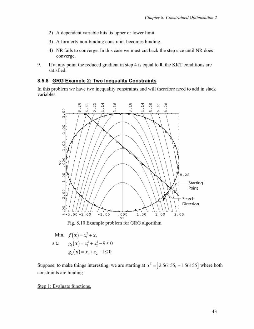
8.5.8 GRG Example 2: Two Inequality Constraints In this problem we have two inequality constraints and will therefore need to add in slack variables.

Fig. 8.10 Example problem for GRG algorithm

Min. ( ) 21 2f x x= +x

s.t.: ( ) 2 21 1 2 9 0g x x= + - £x

( )2 1 2 1 0g x x= + - £x Suppose, to make things interesting, we are starting at [ ]T 2.56155, 1.56155= -x where both constraints are binding. Step 1: Evaluate functions.


44

( ) ( ) ( )1 25.0 0.0 0.0f g g= = =x x x

Step 2: Add in slack variables.

We note that both constraints are binding so we will add in two slack variables. 1 2, s s . Step 3: Partition the variables Since the slack variables are at their lower limits (=0) they will become the independent variables; x1, x2 will be the dependent variables. [ ]T

1 2s s=z [ ]T1 2x x=y

Step 4: Compute the reduced gradient ( ) [ ]T 0.0 0.0fÑ =z ( ) [ ]T 5.123 1.0fÑ =y

1 00 1

y é ù¶= ê ú¶ ë ûz

5.123 3.1231.0 1.0

y -é ù¶= ê ú¶ ë ûy

1 0.1213 0.3787

0.1213 0.6213y - é ù¶

= ê ú-¶ ë ûy

thus 1 0.1213 0.3787 1 0 0.1213 0.3787

0.1213 0.6213 0 1 0.1213 0.6213y y- é ù é ù é ù¶ ¶

= =ê ú ê ú ê ú- -¶ ¶ ë û ë û ë ûy z

[ ] [ ]

[ ] [ ][ ]

T 0.1213 0.37870.0 0.0 5.123 1

0.1213 0.6213

0.0 0.0 0.50 2.56

0.50 2.56

rfé ù

Ñ = - ê ú-ë û= -

= - -

Step 5: Calculate a search direction. We want to move in the negative gradient direction, so our search direction will be

[ ]T 0.50 2.56=s . This is the direction for the independent variables (the slacks). When

normalized this direction is [ ]T 0.19 0.98=s . Step 6: Conduct the line search in the independent variables We will start our line search, denoting the current point as 0z , 1 0 0a= +z z s Suppose we pick a = 1.0. Then


45

( )1

1

0.0 0.191.0

0.0 0.98

0.190.98

é ù é ù= +ê ú ê úë û ë ûé ù

= ê úë û

z

z

Step 7: Adjust the dependent variables To find the change in the dependent variables, we use (7.52)

1

1

2

xx

y y-D é ùé ù ¶ ¶é ùD = = - Dê úê ú ê úD ¶ ¶ë ûë û ë ûy z

y z

0.1213 0.3787 0.190.1213 0.6213 0.98

é ù é ù= ê ú ê ú-ë û ë û

0.3940.586-é ù

= ê ú-ë û

1112

2.56155 0.394 2.168

1.56155 0.586 2.148

xx= - =

= - - = -

at which point ( ) 2.522f =x Have we violated any constraints? ( ) ( ) ( )2 22 2

1 1 2 9 2.168 2.148 9 0.31g x x= + - = + - - =x (violated) ( )2 1 2 1 2.168 2.148 1 0.98g x x= + - = - - = -x (satisfied) We need to drive back to where the violated constraint is satisfied. We will use NR to do this. Since we don't want to drive back to where both constraints are binding, we will set the residual for constraint 2 to zero. NR Iteration 1:

( ) ( )1

0 ( )n y -¶= - -

¶y y g b

y

2.168 0.1213 0.3787 0.312.148 0.1213 0.6213 0.0

2.1302.110

é ù é ù é ù= -ê ú ê ú ê ú- -ë û ë û ë ûé ù

= ê ú-ë û

at this point


46

( ) ( )2 21

2

2.130 2.110 9 0.0110.98

gg= + - = -

= -

NR Iteration 2:

2.130 0.1213 0.3787 0.0112.110 0.1213 0.6213 0.0

2.1313

2.113

-é ù é ù é ù= -ê ú ê ú ê ú- -ë û ë û ë ûé ù

= ê ú-ë û

evaluating constraints:

( ) ( )2 21

2

2.1313 2.113 9 00.98

gg= + - - =

= -

We are now feasible again. We have taken one step in the line search!

Our new point is 2.1313

2.113

é ù= ê ú-ë ûx at which point the objective is 2.43, and all constraints are

satisfied. We would continue the line search until we run into a new constraint boundary, a dependent variable hits a bound, or we can no longer get back on the constraint boundaries (which is not an issue in this example, since the constraint is linear).

Documents

CONSTRAINED OPTIMIZATION 2: SEQUENTIAL QUADRATIC ...apmonitor.com/me575/uploads/Main/chap8_constrained_opt_sqp_ip_grg_v2.pdf · linear constraints is known as a quadratic programming