São Paulo Vehicle Activity Study

Conducted April 12 - 23, 2004 Report Submitted August 20, 2004

James Lents, jlents@issrc.org Nicole Davis, ndavis@issrc.org

International Sustainable Systems Research (http://www.issrc.org) 21573 Ambushers St., Diamond Bar, CA 91765, USA

Nick Nikkila, mail@gssr.net

Global Sustainable Systems Research (http://www.gssr.net/) 7146 Aloe Court, Rancho Cucamonga, CA 91739, USA

Mauricio Osses, maosses@ing.uchile.cl

University of Chile (http://www.uchile.cl) Department of Mechanical Engineering, Casilla 2777, Santiago, Chile

ii

Table of Contents

EXECUTIVE SUMMARY

I. INTRODUCTION..............................................................................................................................................1 II. VEHICLE TECHNOLOGY DISTRIBUTION...............................................................................................3

II.A. BACKGROUND AND OBJECTIVES .................................................................................................................3 II.B. METHODOLOGY...........................................................................................................................................3 II.C. RESULTS......................................................................................................................................................8

II.C.1. Fleet Composition.............................................................................................................................8 II.C.2. Passenger Vehicle Technology Distribution ...................................................................................10 II.C.3. Passenger Vehicle Use....................................................................................................................12 II.C.4. Taxi Survey......................................................................................................................................15 II.C.5. Truck and Bus Survey .....................................................................................................................16

III. VEHICLE DRIVING PATTERNS............................................................................................................19 III.A. BACKGROUND AND OBJECTIVES................................................................................................................19 III.B. METHODOLOGY.........................................................................................................................................19 III.C. RESULTS ....................................................................................................................................................21

III.C.1. Passenger Cars ...............................................................................................................................23 III.C.2. Motorcycles.....................................................................................................................................24 III.C.3. Taxis................................................................................................................................................25 III.C.4. Buses ...............................................................................................................................................26 III.C.5. Trucks..............................................................................................................................................27 III.C.6. Summary of Driving Pattern Results...............................................................................................28

IV. VEHICLE START PATTERNS................................................................................................................33 IV.A. BACKGROUND AND OBJECTIVES................................................................................................................33 IV.B. METHODOLOGY.........................................................................................................................................33 IV.C. RESULTS ....................................................................................................................................................33

V. IVE APPLICATION AND EMISSIONS RESULTS....................................................................................37 V.A. CARBON MONOXIDE...................................................................................................................................39 V.B. VOLATILE ORGANIC COMPOUNDS..............................................................................................................40 V.C. NITROGEN OXIDES .....................................................................................................................................41 V.D. PARTICULATE MATTER ..............................................................................................................................42 V.E. EMISSIONS CONTRIBUTION BY VEHICLE TYPE ............................................................................................43 V.F. EMISSION RATE COMPARISON....................................................................................................................44 V.G. VEHICLE ANNUAL EMISSIONS COMPARISON ..............................................................................................45 V.H. CONCLUSIONS............................................................................................................................................47

APPENDIX A DATA COLLECTION PROGRAM USED IN SÃO PAULO .....................................................................A.1 APPENDIX B ESTUDO DE ATIVIDADE DE FONTES MÓVEIS NA RMSP .................................................................B.1

iii

iv

EXECUTIVE SUMMARY São Paulo, Brazil, was visited from April 12, 2004 to April 23, 2004 to collect and analyze data related to on-road transportation. The study effort was designed to support estimates of the air pollution impacts of on-road transportation in São Paulo that will be used in the development of air quality management plans for the region. It is also hoped that the collected data can be extrapolated to other Brazilian cities to support environmental improvement efforts in these cities as well. The data collection effort was a partnership between the Secretaria de Estado do Meio Ambiente de São Paulo, Companhia de Tecnologia de Saneamento Ambiental (CETESB), and the International Sustainable Systems Research Center (ISSRC) in cooperation with the University of California at Riverside (UCR) and the University of Chile (UCH). The Hewlett Foundation provided technical and financial support. In all, about thirty persons participated in data collection activities over an approximate two week period. The study collected three types of information on vehicles operating on São Paulo streets: technology distribution, driving patterns, and start patterns. Each area is summarized below. Vehicle Technology Distribution

Objective: To develop a representative distribution of vehicle types, sizes, and ages of the operating fleet in the São Paulo area on various roadway types. Methodology: The technology distribution of vehicles was developed using a combination of two approaches. Vehicles were video taped on a variety of streets and the video tapes were reviewed to count the numbers of the various types of vehicles plying São Paulo streets. Simultaneous with this data collection process, parking areas were surveyed to collect specific technology information about vehicles operating in São Paulo. Results: The observed vehicle class fraction for the city overall is shown in Table 1. The amount of driving from passenger cars in São Paulo is similar to the fractions observed in Mexico City (74%) and Santiago, Chile (79%). São Paulo has a high number of motorcycles on the streets, when compared with many other cities where the IVE methodology has been applied, being second after Pune, India, where 55% was found to be 2-wheeler type vehicles.

Table 1: Observed Vehicle Class Distributions in São Paulo, Brazil

Type of Vehicle Observed Travel, 2003

Passenger Car 75.6% Taxi 4.5%

Motorcycle 10.1% Bus 5.3%

Truck 4.5% Total 100%

1

In addition to observing the class distribution, a separate survey was conducted to determine the emissions control technology and engine type of the passenger fleet. It was observed that 20% of the passenger vehicles have no catalyst, and the rest is mainly fitted with three way catalysts. There is some evidence suggesting that a non-determined number of vehicles in São Paulo have their catalytic converter tampered or replaced by inoperative converters. This issue needs further work to be done in order to determine the magnitude of this practice and its impact on emission estimates. The majority of private passenger vehicles on the road are gasoline fueled (92.7%) and there is a fraction mainly comprised by taxis using pure alcohol as fuel (6.7%). It should be noted that even regular gasoline in Brazil contains 25% alcohol.

Vehicle Driving Patterns

Objectives: To collect second-by-second information on the speed and acceleration of the main types of vehicles operating in São Paulo on a representative set of roadways throughout the day. Methodology: The driving patterns for the various classes of vehicles were measured using Global Positioning Satellite (GPS) technology. This technology allows for second by second measurements of vehicle speeds and altitude. GPS units were carried on nine selected routes. Data was collected from 07:00 to 20:00 to provide driving pattern information for differing times of the day. Results: Driving pattern data was successfully collected over 6 days from a number of passenger vehicles, taxis, motorcycles, buses and delivery trucks. Overall, various road types and vehicle types have similar average velocities. It is interesting that the highest and lowest velocities occur on the highways, the highest speeds during the very early morning hours and lowest speeds in the middle of the day, when average speeds are even lower than on residential roadways. Delivery trucks maintain a relatively low average speed throughout the day due to the idle time during deliveries. Buses and taxis have similar average speeds to passenger vehicles traveling on arterial and residential roadways. Taxis and passenger vehicles operating on the highway during the middle of the day and evening exhibit the highest occurrences of hard accelerations, due to congestion and high target speeds.

Vehicle Start Patterns

Objective: To collect a representative sample of the number, time of day, and soak period from passenger vehicles operating in São Paulo. Methodology: The vehicle engine start patterns were collected using equipment that senses vehicle system voltage denoted VOCE units. VOCE data can be used to determine when vehicles start, how long they operate, and how long they sit idle between starts. This information is essential to establish vehicle start emissions. The VOCE units were placed in passenger vehicles and left there for a period of a week.

2

Results: Over 330 days of start patterns were collected from 69 different vehicles over the study period. The results show that on average, a typical passenger car is started 6.1 times per day. Approximately 25% of the starts occur between 10 am and 13:59 pm, and another 24% occur between 16 pm and 19:59 pm. In the early morning hours, over half of the starts occur after having rested for over 12 hours. These long soaks leave the engine cold, which results in increased starting emissions.

Conclusions

The three types of data collected in this study have been used to compile a comprehensive analysis of the make-up and behavior of the current on-road mobile fleet in São Paulo. This data is pertinent for correctly estimating current mobile source emissions and projecting the impact of proposed control strategies and growth scenarios, because the vehicle type, speed profiles, and the number of starts and the soak period have a large impact on the mobile source emissions inventory. The data collected in this study was formatted to allow vehicle emissions estimates using the International Vehicle Emissions Model (http://www.issrc.org/ive or www.gssr.net/ive). The IVE model was developed with USEPA funding to make emissions estimates under different technology and driving situations as found in various countries, and has been used extensively in several developing countries. Although up-to date vehicle activity and fleet information was collected in this study, no emissions measurements were made. All emission estimates conducted using the IVE model’s default emission rates. It is planned that some emission measurements will be conducted with on-road vehicles to create São Paulo specific emission rates. Overall, the results of this study have shown that driving in São Paulo is similar to other developing urban areas with some subtle but important differences. The number of starts per day and the kilometers driven per day per passenger vehicle is slightly lower than seen in other areas researched to date. The average age of the passenger fleet and average mileage accumulation varies widely from city to city in the countries studied to date, but São Paulo falls in the middle of this range for both variables. São Paulo’s passenger fleet is comprised of approximately 20% non catalyst vehicles, compared to 1% in the US; 20-30% in Mexico City, Santiago, and Pune; and 90-100% in Almaty and Nairobi. A preliminary emissions analysis using the IVE model indicate that on the order of 45 metric tons of PM, 1168 tons of NOx, 855 tons of VOC, and 8215 tons/day of CO are emitted from on-road motor vehicles each day in São Paulo Metropolitan Region (SPMR)1. By viewing the contribution of various vehicle types to the inventory, it was determined that to reduce PM (and toxic) emissions in São Paulo, buses and trucks must be controlled. To reduce NOx, buses, trucks, and passenger vehicles must be further controlled. All of these types of vehicles in the São Paulo fleet have better emissions control alternatives that could be employed to reduce emissions. It must be noted again that the emissions analysis is subject to the appropriateness of the emission rates used in the IVE model.

1 This calculation was made considering a total registered fleet of 7,653,881 vehicles in SPMR, reported by the State Traffic Department, January 2004 (DETRAN-SP).

3

Several recommendations for additional study include using the tools outlined in this report to develop a strategy for improving future air quality, determine the appropriateness of the collected data to suburban areas outside of São Paulo or other urban areas within Brazil, and improve the emission factors for in-use vehicles. An improved estimate of current overall vehicular travel (VKT) and future growth rates is also recommended.

4

I. INTRODUCTION The vehicle activity study was conducted in São Paulo, Brazil, from December 1, 2003 to December 15, 2003. During this time, in cooperation with local universities and government officials, three types of information were collected. Subsequently, this data was processed and analyzed and put into a format to be used in the IVE model. The data, collection process, comparisons with other areas studied, and emissions results from the IVE modeled are reported in this paper. The data collected has three purposes:

• To estimate the technology distribution of vehicles operating on São Paulo streets. • To measure driving patterns for the various classes of vehicles operating on São Paulo

streets. • To estimate the times and numbers of vehicle engine starts for the various classes of vehicles

operating on São Paulo streets. The technology distribution of vehicles was developed using a combination of two approaches. Vehicles were video taped on a variety of streets and the video tapes were reviewed to count the numbers of the various types of vehicles plying São Paulo streets. Simultaneous with this data collection process, parking areas were surveyed to collect specific technology information about vehicles operating in São Paulo. The driving patterns for the various classes of vehicles were measured using Global Positioning Satellite (GPS) technology. This technology allows for the second by second measurements of vehicle speeds. GPS units were carried on a variety of vehicles on a variety of street types throughout the metropolitan area. Data was collected from 07:00 to 20:00 to provide driving pattern information for differing times of the day. The vehicle engine start patterns were collected using equipment that senses vehicle system voltage denoted VOCE units. VOCE data can be used to determine when vehicles start, how long they operate, and how long they sit idle between starts. This information is essential to establish vehicle start emissions. The data collected in this study was formatted to allow vehicle emissions estimates using the International Vehicle Emissions Model (http://www.issrc.org/ive or www.gssr.net/ive). This model was developed with USEPA funding to make emissions estimates under different technology and driving situations as found in various countries. Each process and results are described in detail in the next sections.

1

2

II. VEHICLE TECHNOLOGY DISTRIBUTION II.A. BACKGROUND AND OBJECTIVES The most critical element of on-road transportation emissions analysis is the nature of the vehicle technologies that operate on the street or in the region of interest. Different vehicle technologies can produce considerably different rates of emissions. Vehicles operating on the same roads can produce emissions that are 300 times different from one another. The fractions of various types of vehicles in a local fleet and the fractions of these various types of vehicles actually operating on the roadways are not necessarily the same. This difference occurs because some classes of vehicles are operated considerably more than other classes of vehicles. For example, a class of vehicles that operates twice as much as another class will produce an on-road fraction that is twice as great even if there are equal numbers of vehicles in the static fleet. The fraction of interest for estimating on-road emissions is the fraction of driving contributed by the various vehicle technologies since this will correspond to the amount of air emissions that are produced. Thus, the most accurate estimate of vehicular contribution to air emissions is made by determining the fractions of the various vehicle technology classes actually operating on city streets rather than the distribution of vehicles registered in the region of interest. The objective of this portion of the study is to develop a representative distribution of vehicle types, sizes, and ages of the operating fleet in the São Paulo area on various roadway types through a passenger survey. The goal of the survey was to identify the specific engine technologies, drive train, control technologies, air conditioning, total use, and model years of the vehicles surveyed. II.B. METHODOLOGY Three representative sections of the city under analysis are normally selected for the IVE activity study. The areas selected should represent the fleet makeup and the general driving taking place in the city. To accomplish this objective, one of the study areas is selected to be representative of the lower income areas of the city, another area represents a generally upper income area of the city, and the third one represents a commercial area of the city - normally the city center. On-road driving varies by the time of the day, by the day of the week, and by the location in an urban area. To account for this, during the IVE study, data is collected at different times of the day and in different locations within an urban area. In order to insure that the most representative data is collected, both video-traffic and parked vehicle studies were carried out from 07:00 in the morning to 20:00 in the evening over 6 days in 3 representative sections of the urban area. Surveys were carried out on or near (in the cases of parked vehicle surveys) a residential street, an arterial roadway, and a highway in each area surveyed. Table II.1 indicates the locations in São Paulo where video surveys were completed: Campo Limpo/Capão Redondo (low income), Alto de Pinheiros (high income) and 23 de Maio/Jardins (commercial). These locations were suggested by the São Paulo city officials as representative of the general urban area. They also represent the locations were driving patterns were measured. Parking surveys were completed at locations generally in the vicinity of the video surveys.

3

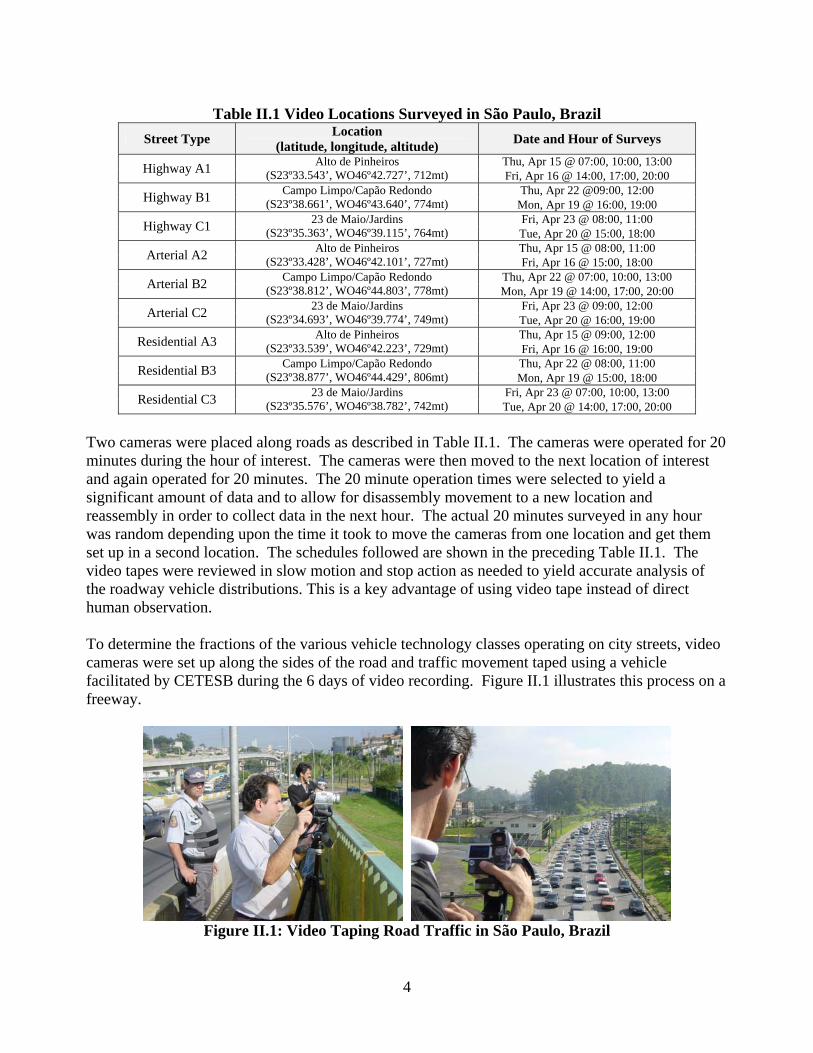
Table II.1 Video Locations Surveyed in São Paulo, Brazil

Street Type Location (latitude, longitude, altitude) Date and Hour of Surveys

Thu, Apr 15 @ 07:00, 10:00, 13:00 Highway A1 Alto de Pinheiros (S23º33.543’, WO46º42.727’, 712mt) Fri, Apr 16 @ 14:00, 17:00, 20:00

Thu, Apr 22 @09:00, 12:00 Highway B1 Campo Limpo/Capão Redondo (S23º38.661’, WO46º43.640’, 774mt) Mon, Apr 19 @ 16:00, 19:00

Fri, Apr 23 @ 08:00, 11:00 Highway C1 23 de Maio/Jardins (S23º35.363’, WO46º39.115’, 764mt) Tue, Apr 20 @ 15:00, 18:00

Thu, Apr 15 @ 08:00, 11:00 Arterial A2 Alto de Pinheiros (S23º33.428’, WO46º42.101’, 727mt) Fri, Apr 16 @ 15:00, 18:00

Thu, Apr 22 @ 07:00, 10:00, 13:00 Arterial B2 Campo Limpo/Capão Redondo (S23º38.812’, WO46º44.803’, 778mt) Mon, Apr 19 @ 14:00, 17:00, 20:00

Fri, Apr 23 @ 09:00, 12:00 Arterial C2 23 de Maio/Jardins (S23º34.693’, WO46º39.774’, 749mt) Tue, Apr 20 @ 16:00, 19:00

Thu, Apr 15 @ 09:00, 12:00 Residential A3 Alto de Pinheiros (S23º33.539’, WO46º42.223’, 729mt) Fri, Apr 16 @ 16:00, 19:00

Thu, Apr 22 @ 08:00, 11:00 Residential B3 Campo Limpo/Capão Redondo (S23º38.877’, WO46º44.429’, 806mt) Mon, Apr 19 @ 15:00, 18:00

Fri, Apr 23 @ 07:00, 10:00, 13:00 Residential C3 23 de Maio/Jardins (S23º35.576’, WO46º38.782’, 742mt) Tue, Apr 20 @ 14:00, 17:00, 20:00

Two cameras were placed along roads as described in Table II.1. The cameras were operated for 20 minutes during the hour of interest. The cameras were then moved to the next location of interest and again operated for 20 minutes. The 20 minute operation times were selected to yield a significant amount of data and to allow for disassembly movement to a new location and reassembly in order to collect data in the next hour. The actual 20 minutes surveyed in any hour was random depending upon the time it took to move the cameras from one location and get them set up in a second location. The schedules followed are shown in the preceding Table II.1. The video tapes were reviewed in slow motion and stop action as needed to yield accurate analysis of the roadway vehicle distributions. This is a key advantage of using video tape instead of direct human observation. To determine the fractions of the various vehicle technology classes operating on city streets, video cameras were set up along the sides of the road and traffic movement taped using a vehicle facilitated by CETESB during the 6 days of video recording. Figure II.1 illustrates this process on a freeway.

Figure II.1: Video Taping Road Traffic in São Paulo, Brazil

4

Figure II.2 illustrates the same process on a residential street (left) and one of the arterial streets (right) in São Paulo, Brazil.

Figure II.2: Video Taping Road Traffic in São Paulo, Brazil

The completed videotapes were analyzed in slow motion to insure the most accurate counts of vehicles, as it is shown in Figure II.3. These videotapes were reviewed to determine the numbers of passenger vehicles, taxis, buses (small, medium and large), trucks (small, medium and large), motorcycles, three-wheeled vehicles, and other vehicles observed on the nine city streets. The traffic volumes were also determined.

Figure II.3: Video Tape Counting at CETESB, São Paulo, Brazil

Table II.2 shows examples of the different vehicle categories considered in this study.

5

Table II.2: Examples of Fleet Distribution by Vehicle Category Vehicle category Examples

Passenger vehicle

Taxi

Small truck

Medium truck

Large truck

Small bus

Medium bus

6

Large bus

Motorcycle

It is not normally possible using the video taping process to determine the exact nature of the vehicle technologies observed. The video taping allowed the determination of the fractions of trucks, buses, passenger vehicles, 2-wheelers, and such operating on the roadways of interest. To understand the specific technologies of passenger vehicles, parking surveys were completed. Parked vehicle surveys allow careful inspection of vehicles so that the engine technology, model year, control equipment, and fuel type can be established. The parked vehicle surveys were used to estimate the more specific natures of the general vehicle classifications determined from the video tape studies. Two teams of students were used in the parking lot survey in São Paulo. One team was experienced with respect to vehicle technologies and the other group was experienced with respect to survey methodologies. The two teams worked the same areas each day following the schedule and locations selected for video tape recordings (Table II.1). Figure II.3 shows the actual parking lot survey process in São Paulo, Brazil.

Figure II.3: Parking Lot Survey in São Paulo, Brazil

7

The data collected in the parking lot studies consisted of vehicle manufacturer, model, fuel type, model year, license plate number, engine size and technology, odometer reading, add-on control technology, transmission type, air conditioning, and general condition. The data collected during the survey was processed onto a database and the students that were involved in the study received a certificate for their participation.

Figure II.4: Parking Lot Data Processing and Certificates for Students

II.C. RESULTS II.C.1. Fleet Composition A total of 840 minutes (14 hours) of digital video were recorded throughout the 6-days of field work in São Paulo. These 14 hours of video recording are representative of 42 hours of traffic activity, when each period of 20 minutes of traffic counts is expanded into an hour. As can be seen in Table II.3 (below and next page), the distribution of vehicles varies with street type and time of day. Thus, for highly time and street specific analysis, care must be taken to construct a proper technology distribution for the time and street of interest. For this analysis, overall average technology distributions are developed for the general metropolitan area.

Table II.3: Results of Analysis of São Paulo Videotapes Area Time Pass.

car Taxi Small truck

Medium truck

Large truck

Small bus

Medium bus

Large bus

Motor cycles

Vehicles /hour

A 06:00-13:00 71.2% 4.2% 1.6% 1.9% 5.9% 4.1% 0.2% 1.0% 9.9% 3220 A 13:00-20:00 77.9% 2.8% 0.5% 1.5% 3.7% 3.3% 0.1% 1.2% 9.0% 3052 B 06:00-13:00 69.8% 3.5% 0.5% 1.5% 3.1% 4.5% 1.9% 2.5% 12.7% 1981 B 13:00-20:00 72.2% 2.6% 0.9% 1.5% 2.7% 4.6% 2.2% 2.8% 10.5% 1616 C 06:00-13:00 78.5% 6.0% 0.9% 0.6% 0.3% 3.2% 0.0% 0.9% 9.7% 3437 C 13:00-20:00 79.6% 6.2% 0.3% 0.5% 0.3% 2.5% 0.1% 0.6% 9.9% 3503

Total 06:00-13:00 73.8% 4.8% 1.1% 1.3% 3.0% 3.8% 0.5% 1.3% 10.5% 2879 Total 13:00-20:00 77.5% 4.2% 0.5% 1.1% 2.0% 3.2% 0.5% 1.3% 9.7% 2724

Grand Total All Day 75.6% 4.5% 0.8% 1.2% 2.5% 3.5% 0.5% 1.3% 10.1% 2801

8

Table II.3: Results of Analysis of São Paulo Videotapes (cont.) Road type Area Time Pass.

car Taxi Small truck

Medium truck

Large truck

Small bus

Medium bus

Large bus

Motor cycles

Vehicles /hour

Highway A1 7:00 75.8% 0.5% 1.0% 3.1% 12.2% 3.3% 0.1% 0.4% 3.5% 5967 Highway A1 10:00 63.4% 1.2% 1.3% 3.3% 14.1% 5.9% 0.1% 0.2% 10.4% 6850 Highway A1 13:00 66.3% 1.7% 1.1% 2.8% 12.1% 5.4% 0.1% 0.3% 10.3% 6528 Highway A1 14:00 63.9% 2.0% 0.8% 3.3% 12.4% 6.1% 0.2% 0.3% 10.9% 7034 Highway A1 17:00 66.4% 1.4% 1.0% 2.9% 8.4% 3.4% 0.1% 0.3% 16.1% 4790 Highway A1 20:00 78.7% 0.4% 2.3% 1.9% 10.6% 2.7% 0.0% 0.4% 3.0% 5283 Highway B1 9:00 79.0% 4.5% 0.8% 1.4% 4.9% 4.2% 0.1% 0.9% 4.2% 4379 Highway B1 12:00 70.4% 2.5% 0.9% 3.2% 8.0% 5.7% 0.2% 1.7% 7.5% 3570 Highway B1 16:00 67.3% 2.9% 1.2% 4.6% 5.2% 5.1% 0.3% 1.5% 11.9% 3509 Highway B1 19:00 82.1% 1.6% 0.3% 1.6% 2.8% 3.4% 0.2% 1.0% 7.1% 3642 Highway C1 8:00 83.7% 5.2% 0.4% 0.2% 0.0% 2.6% 0.0% 0.6% 7.3% 6207 Highway C1 11:00 73.8% 5.5% 0.9% 0.3% 0.2% 4.8% 0.0% 0.2% 14.3% 6201 Highway C1 15:00 81.4% 5.1% 0.6% 0.4% 0.1% 2.1% 0.1% 0.2% 10.0% 10018 Highway C1 18:00 64.9% 10.0% 0.2% 0.0% 0.1% 2.1% 0.0% 0.2% 22.7% 3506

Arterial A2 8:00 83.5% 3.8% 1.2% 0.9% 1.7% 2.4% 0.7% 4.0% 1.9% 1270 Arterial A2 11:00 74.6% 6.2% 0.9% 1.6% 0.5% 4.3% 0.4% 2.0% 9.6% 1686 Arterial A2 15:00 76.6% 4.7% 0.2% 1.3% 0.3% 4.4% 0.3% 1.7% 10.5% 1922 Arterial A2 18:00 87.4% 2.4% 0.1% 0.4% 0.0% 1.4% 0.0% 1.5% 6.7% 2138 Arterial B2 7:00 56.5% 2.3% 0.0% 0.2% 1.0% 3.1% 4.6% 5.1% 27.2% 1814 Arterial B2 10:00 57.0% 2.5% 0.9% 2.3% 3.9% 7.2% 5.5% 5.5% 15.0% 1300 Arterial B2 13:00 64.9% 2.4% 0.6% 2.0% 1.6% 6.9% 4.1% 5.7% 11.8% 1520 Arterial B2 14:00 67.9% 2.7% 0.6% 2.1% 3.6% 5.7% 4.2% 4.4% 8.9% 1574 Arterial B2 17:00 68.9% 1.6% 0.3% 0.5% 1.8% 6.0% 6.3% 6.8% 7.8% 1149 Arterial B2 20:00 61.1% 2.1% 1.7% 0.0% 3.0% 4.7% 10.7% 9.8% 6.8% 703 Arterial C2 9:00 74.8% 8.6% 1.0% 0.5% 0.5% 3.5% 0.0% 1.3% 9.9% 1774 Arterial C2 12:00 73.0% 6.7% 1.2% 0.8% 0.2% 3.6% 0.0% 1.2% 13.3% 1925 Arterial C2 16:00 77.2% 7.2% 0.2% 0.5% 0.4% 2.3% 0.1% 1.2% 10.8% 2840 Arterial C2 19:00 85.2% 5.5% 0.3% 0.3% 0.3% 1.8% 0.0% 1.3% 5.5% 2138 Arterial C3 7:00 89.2% 4.3% 0.3% 0.2% 0.0% 1.9% 0.0% 1.2% 3.1% 3242 Arterial C3 10:00 77.8% 5.8% 1.4% 1.2% 0.8% 2.5% 0.0% 0.4% 10.1% 2278 Arterial C3 13:00 79.3% 5.4% 1.1% 1.2% 0.4% 2.8% 0.2% 0.9% 8.6% 2431 Arterial C3 14:00 76.1% 7.8% 0.1% 0.9% 0.6% 5.2% 0.0% 0.6% 8.6% 2299 Arterial C3 17:00 80.4% 3.6% 0.3% 0.6% 0.6% 3.4% 0.0% 0.4% 10.8% 2122 Arterial C3 20:00 89.5% 5.2% 0.2% 0.6% 0.2% 0.7% 0.2% 0.6% 2.8% 1598

Residential A3 9:00 72.2% 5.6% 0.0% 0.0% 2.8% 5.6% 0.0% 0.0% 13.9% 108 Residential A3 12:00 62.8% 7.0% 4.7% 2.3% 4.7% 2.3% 0.0% 0.0% 16.3% 128 Residential A3 16:00 69.7% 9.1% 0.0% 0.0% 3.0% 9.1% 0.0% 0.0% 9.1% 99 Residential A3 19:00 87.5% 6.3% 0.0% 0.0% 0.0% 3.1% 0.0% 0.0% 3.1% 96 Residential B3 8:00 74.4% 4.9% 0.0% 0.3% 0.9% 3.2% 1.2% 0.6% 14.5% 1041 Residential B3 11:00 76.8% 2.4% 1.2% 3.7% 1.2% 2.4% 0.0% 2.4% 9.8% 246 Residential B3 15:00 72.1% 5.4% 2.7% 0.9% 1.8% 2.7% 0.0% 0.0% 14.4% 334 Residential B3 18:00 77.3% 1.5% 0.0% 0.0% 0.8% 5.3% 0.0% 1.5% 13.6% 399

Grand Total All Day 75.6% 4.5% 0.8% 1.2% 2.5% 3.5% 0.5% 1.3% 10.1% 2801

The vehicle technology distributions varied among the different studied cities, and also there are some remarkable similarities. Table II.4 compares general vehicle mixes observed on city streets in eight cities where the IVE methodology to determine vehicle activity has been applied.

9

Table II.4: Comparison of Observed Fleet Mix in Urban Areas Worldwide

City Passenger Vehicles

Motor Cycles Taxi 3-Wheel

Carriers Small Buses

Medium / Large Buses

Small / Medium Delivery Trucks

Large (18 Wheel Type)

Trucks

Non-Motorized

Almaty, Kazakhstan 83% 0% 0% 0% 9% 3% 5% 0% 1% Lima, Peru 52% 1% 3% 0% 15% 3% 5% 1% 0%

Los Angeles, USA 95% 0% 0% 0% 0% 1% 1% 3% 0%

Mexico City, Mexico 74% 2% 15% 0% 2% 1% 4% 1% 0% Nairobi, Kenya 88% 2% 1% 0% 2% 2% 4% 1% 1%

Pune, India 12% 55% 0% 13% 0% 1% 1% 0% 17%

Santiago, Chile 79% 1% 8% 0% 0% 6% 5% 1% 0%

São Paulo, Brazil 75% 10% 5% 0% 3% 2% 2% 3% 0%

II.C.2. Passenger Vehicle Technology Distribution A total of 1427 passenger cars were surveyed in parking lots located near the areas where the CPGS equipped cars were following their routes. Table II.5 indicates some of the general characteristics observed in the surveyed fleet.

Table II.5: General characteristics of the surveyed Passenger Cars Type of Fuel* Air Conditioning System Type of Transmission Catalytic Converter (CC)**

92.7% Gasoline 67.9% with A/C 97.3% Mechanic Trans. 19.4% without CC 6.7% Alcohol 32.1% without A/C 2.7% Automatic Trans. 80.6% with CC

*0.4% diesel and 0.2% LPG and gasoline (dual engines) **Considering only gasoline vehicles then 13.9% without CC and 86.1% with CC

There is some evidence suggesting that a non-determined number of vehicles in São Paulo have their catalytic converter tampered or replaced by inoperative converters. This report does not consider any tampering or replacement of catalytic converter on the emission calculation process. However, this issue needs further work to be done in order to better determine the magnitude of this practice and its impact on emission estimates. The IVE Model defines 1328 technology classifications based on fuel type, engine technology, and control technology plus 45 user defined technologies. An example of six technology types for gasoline passenger vehicles is shown in Table II.6, indicating that 86% of the gasoline passenger cars in São Paulo are equipped with catalytic converter and that a vast majority (77.6%) is fitted with multipoint fuel injection system.

Table II.6: IVE technology fractions of the Gasoline Passenger Cars

Passenger Vehicles Fraction of Passenger Vehicles

Gasoline, 4-stroke, Carburetor, No Catalyst 9.5% Gasoline, 4-stroke, Carburetor, 2-way Catalyst 1.7%

Gasoline, 4-stroke, Single Point Fuel Injection, No Catalyst 3.9% Gasoline, 4-stroke, Single Point Fuel Injection, 3-way Catalyst 6.7%

Gasoline, 4-stroke, Multipoint Fuel Injection, No Catalyst 0.5% Gasoline, 4-stroke, Multipoint Fuel Injection, 3-Way Catalyst 77.6%

10

In addition to the gasoline cars shown in the Table II.6 above, 95 out of 1427 vehicles used alcohol as fuel, most of them without a catalytic converter and carbureted (92%). The emissions control system on passenger vehicles in São Paulo is similar to Mexico City and Santiago, where high fractions of three-way catalyst vehicles were found. In contrast, Almaty has mostly non-catalyst vehicles (Table II.7) and Nairobi has in effect no catalyst due to the use of leaded gasoline. Los Angeles has the highest fraction of cars fitted with 3-way catalyst and fuel injection control system.

Table II.7: Current Passenger Vehicle Technology Distributions around the World Air/Fuel Control Catalyst

Location Carburetor Fuel Injection None 2-Way Catalyst

3-Way Catalyst

Almaty, Kazakhstan 45% 51% 89% 0% 7% Lima, Peru 44% 56% 53% 6% 40%

Los Angeles, USA 6% 94% 1% 3% 96% Mexico City, Mexico 18% 82% 20% 0% 80%

Nairobi, Kenya 60% 32% 100% 0% 0% Pune, India 42% 32% 29% 35% 11%

Santiago, Chile 17% 80% 17% 3% 77% São Paulo, Brazil 17% 83% 19% 0% 81%

Table II.8 indicates the engine size and use distribution of the passenger vehicle in São Paulo.

Table II.8: Size and Use Characteristics of the Surveyed Passenger Car Fleet Vehicle Engine Size 67.3% Low Use

(<80 K km) 29.7% Medium Use

(80-161 K km) 3.0% High Use (>161 K km)

52% Small (<1301 cc) 38.2% 12.6% 1.3% 45% Medium (1301-2000 cc) 27.4% 16.1% 1.4%

3% Large (>2000 cc) 1.8% 1.1% 0.3% The engine size of the São Paulo vehicle fleet was generally small (52% less than 1301cc) and medium (45% greater than 1300cc and less than 2000cc). Table II.6 also shows a very low proportion of vehicles in the higher use category (only 3% greater than 161 K km). This value may be wrong likely due to a common practice of tampering in the odometer readings, especially in older vehicles. This observation will be further discussed in Section II.C.3. Information in Table II.6 must be combined with information in Tables II.8 along with the video collected data in Table II.3 to produce the passenger vehicle information for estimating emissions. Figure II.6 illustrates the model year distribution for active passenger vehicles in São Paulo. The average age of passenger vehicles surveyed during the parking lot activity was 7.37 years.

11

0%

2%

4%

6%

8%

10%

12%

pre19

8119

8319

8519

8719

8919

9119

9319

9519

9719

9920

0120

03

Model year

Frac

tion

of a

ctiv

e pa

ssen

ger c

ars

Figure II.6: Model Year Distribution in the São Paulo Passenger Vehicle Fleet

Figure II.7 illustrates the average age of the on-road vehicle fleet in different cities where the IVE methodology has been carried on.

3.5

4.7

6.4 6.5 6.67.4

11.0 11.3

13.2

0

2

4

6

8

10

12

14

16

Beijin

g, Chin

a

Pune,

India

Mexico

City

, Mex

ico

Santia

go, C

hile

Los A

ngele

s, USA

Sao

Paulo,

Bra

zil

Lima,

Peru

Almaty

, Kaz

akhs

tan

Nairob

i, Ken

ya

Aver

age

Age

[yrs

]

Figure II.7: Comparison of Average Vehicle Age in Different Cities

Average vehicle use in São Paulo is similar but slightly higher than the values obtained in Mexico City, Santiago and Los Angeles. Beijing and Pune have the lower average uses, while Lima, Almaty and Nairobi belong to the higher rated group in this comparison analysis. II.C.3. Passenger Vehicle Use Odometer data was obtained from the parking lot surveys. Thus, some approximation of the use of individual vehicles can be made and this can be extrapolated to make approximations of total vehicle use for São Paulo.

12

Figure II.8 shows the passenger vehicle use taken from vehicle odometers, where each point is the average of the vehicles surveyed at different age groups. According to this trend line, vehicle use during the first year corresponds to 13,644 km with a yearly reduction rate equals to 2.7%.

y = -367.87x2 + 13644xR2 = 0.9364

0

20000

40000

60000

80000

100000

120000

140000

160000

0 2 4 6 8 10 12 14 16 18 20

Age (Years)

Acc

umul

ated

Use

(km

s)

Figure II.8: Passenger Vehicle Use during the first twenty years of age

However, the equation shown in Figure II.8 will produce unreasonable results mainly due to the uncertainty in odometer readings for the older group of vehicles. Statistics from the Ministério dos Transportes2 indicates that average driving for passenger vehicles was 18,000 km/year in 1985 and CETESB staff indicated that new vehicles in São Paulo are currently driving approximately 20,000-22,000 km/year. It may be more appropriate to replace the second order term in the vehicle use equation with a value that is similar in a relative sense to those measured in other countries. Figure II.9 shows the complete set of raw data from the parking lot survey (grey dots), the average for model years 2004-1985 (red dots) and a modified trend line showing the expected driving according to a more representative behavior (alternate driving), considering 20,000 km during first year of driving and a yearly reduction rate equal to 2%.

0

50000

100000

150000

200000

250000

300000

350000

400000

196519701975198019851990199520002005Model year

Odo

met

er re

adin

g [k

m]

Raw Sao Paulo DataAlternate DrivingAverage Driving per Year

Figure II.9: Parking Lot Survey Results and Proposed Driving Curve for São Paulo

2 Ministério dos Transportes, Frota de Veiculos Automotores 1985, Brasilia, 1986.

13

Considering the alternate driving trend line indicated above, it is possible make a comparison between São Paulo and other cities worldwide. Figure II.10 illustrates the total driving per vehicle for the countries studied to date. As can be seen, passenger cars are driven the most in the United States and the least in Pune, India. For the first 15 years of age, the proposed driving curve for São Paulo has a similar mileage pattern for passenger vehicles to the driving observed in Nairobi, Almaty and Beijing.

0

50,000

100,000

150,000

200,000

250,000

300,000

350,000

400,000

0 5 10 15 20 25

Vehicle Age [yr]

Acc

umul

ated

Driv

ing

[km

]

Los AngelesNairobiBeijingAlmatyLimaSantiagoMexico CityPuneSao Paulo

Figure II.10: Comparison of Passenger Vehicle Use in different cities

As is typical for the United States and all other countries studied so far, vehicle use decreases with vehicle age. Using the age distribution illustrated in previous Figure II.6, the average passenger car age in São Paulo is approximately 7.4 years. Considering this figure and from the alternate driving curve, it is possible to estimate an overall average for São Paulo passenger cars equals to 16,991 km/year, thus, an average daily driving of 46.6 kilometers of driving per day over the year (assuming 365 days/year). A comparison of annual driving in several cities is shown below.

0

5,000

10,000

15,000

20,000

25,000

30,000

0 5 10 15 20 25

Vehicle Age [yr]

Ann

ual D

rivin

g [k

m/y

r]

Los AngelesNairobiBeijingAlmatyLimaSantiagoMexico CityPuneSao Paulo

Figure II.11: Comparison of Annual Driving in Different Cities Worldwide

14

The current travel in São Paulo is estimated to be approximately 352,078,526 kilometers per day for passenger cars. This estimate is used in the IVE analysis to project emissions for the whole city. Table II.9 below provides the estimated total driving based on measurements made in this study for all vehicle categories.

Table II.9: Observed Travel Distribution by vehicle type in São Paulo

Type of Vehicle Fraction of

Observed Travel, 2003

Estimated Travel (km/day)

Thousands Passenger Car 75.6% 266,171

Taxi 4.5% 15,844 Motorcycle 10.1% 35,560

Bus 5.3% 18,660 Truck 4.5% 15,843 Total 100.0% 352,078

The values shown in Table II.9 should only be treated as approximations, but they should be in the ballpark of the true total driving occurring in São Paulo Metropolitan Region in 2004. These values have been calculated using the dynamic composition of the fleet obtained from video tape analysis (Table II.3) combined with a total fleet of 7,653,881 vehicles in São Paulo. An average driving of 46.6 km/day/vehicle was used for all vehicle categories, taking the activity of passenger cars as the reference value. II.C.4. Taxi Survey A short survey was carried out with 8 taxi drivers working in São Paulo. The results of these interviews are summarized in the Table below.

Table II.10: Taxi Survey in São Paulo Average Driving Vehicle Age Odometer

Reading Estimated

Annual Driving Taxi No

[km/day] [days/week] [months] [km] [km/year] A 200 6 -- -- 62,400 B 200 6 6 24,400 48,000 C 150 5 14 45,750 39,200 D 150 6 3 14,226 56,900 E 220 7 96 254,594 31,800 F 250 7 36 172,295 57,400 G 150 6 36 121,524 40,500 H 150 6 4 14,390 43,170

One taxi driver indicated that the government gives a tax incentive to taxi owners to buy vehicle but they must only drive a taxi and can not have another job. Also, taxi must run on alcohol. Another taxi driver thinks that taxis get exchanged in about 5 years. If the drivers are correct and taxis are eliminated by 10 years (one taxi driver said 5 years) this means there will be an average of 10%-

15

20% turnover each year. The government gives a tax incentive to buy all alcohol cabs and most cabs do this. This study considers that all taxis in SPRM are running with retrofit systems based on ethanol. II.C.5. Truck and Bus Survey The parking lot survey was not conducted for trucks and buses in São Paulo. Instead, data from CETESB was analyzed to determine the specific engine technologies. Gabriel Bracco reported that São Paulo trucks and buses followed the following emissions schedule:

Table II.11: EURO Standards in São Paulo Standard Truck Bus

Euro 0 Pre 1996 Pre 1994 Euro 1 1996 1994 Euro 2 2000 1998 Euro 3 2004 (70%) 2004 (70%) Euro 3 2005 (80%) 2005 Euro 4 2009 2009

CETESB agrees with this distribution of standards. The most common engine is the 6 liter Mercedes engine. Present diesel fuel is about 1,100 ppm sulfur, in 2006 diesel will be reduced to a maximum of 500 ppm sulfur, and in 2009 diesel will be further reduced to 50 ppm sulfur. In general, there is no good data on technology distribution of trucks in the field. In an attempt to better understand the technology distribution of trucks on the road, one of the digital video cameras was used to collect license plates from trucks. This process was carried out during the last two days of the activity study and complemented by further on-road license plate visual observations carried out by CETESB. Finally, 395 valid license plates were identified and post processed. From this license plate analysis, the following model year distribution was found:

0.0%

1.0%

2.0%

3.0%

4.0%

5.0%

6.0%

7.0%

8.0%

2004

2002

2000

1998

1996

1994

1992

1990

1988

1986

1984

1982

1980

1978

1976

1974

Model Year

Frac

tion

Figure II.12: Model Year Distribution in the São Paulo Truck Fleet

16

According to the model year distribution it can be determined that 40% of the sample (156 trucks) corresponded to EURO 0 standards, 16% to EURO 1 (64 trucks), 37% to EURO 2 (144 trucks), 6% to EURO 3 (24 trucks), and only one truck complied with EURO 4 standards. From the same license plate data base it was found that 63% of the trucks had turbo system, 40% were equipped with intercooler, and only 5% were fitted with electronic injection system. Data from buses was not found and the same technology above distribution based on EURO standards for trucks was used as a reference for calculating emissions. These data can be improved in future fleet analysis.

17

18

III. VEHICLE DRIVING PATTERNS III.A. BACKGROUND AND OBJECTIVES The main objective of this section is to collect second-by-second information on the speed and acceleration of the main types of vehicles operating in São Paulo, on a representative set of roadways throughout the day. III.B. METHODOLOGY Vehicle driving patterns were measured using GPS technology as described in Appendix A. This technology allows the measurement each second of vehicle location, speed, and altitude. Three representative sections of the city were selected for the IVE study in São Paulo. The areas selected represent a generally lower income area (Campo Limpo/Capão Redondo), a generally upper income area (Alto de Pinheiros), and a commercial area of the city (23 de Maio/Jardins). Figure III.1 show the sectors and streets selected in this study.

Figure III.1: Areas and Streets for the IVE Study in São Paulo

19

Figure III.2 shows in more detail the 9 streets selected in this Activity Study where the 3 passenger cars collected driving data over 6 days. A total of 311,323 valid track logs were recorded during the campaign (98,123 in highways; 115,127 in arterials; and 98,073 in residential streets).

-23.68

-23.66

-23.64

-23.62

-23.6

-23.58

-23.56

-23.54

-23.52

-23.5-46.78 -46.76 -46.74 -46.72 -46.7 -46.68 -46.66 -46.64 -46.62

Longitude

Latit

ude

HI-HwyHI-Art

HI-ResLI-HwyLI-Art

LI-ResC-Hwy

C-Art1C-Art2

Figure III.2: São Paulo Routes for Collecting Passenger Cars Driving Patterns

A total of 11 GPS units were used in the activity study in São Paulo: 3 of them collected driving data in passenger cars, 2 were for buses, 2 for trucks, 2 for taxis and 2 for a motorcycle (a smaller prototype GPS unit was tested by the motorcycle driver). Figure III.3 shows some examples of the installation of these units during the São Paulo field work.

Figure III.3: Examples of GPS Units Installation in a Motorcycle, Bus, Truck and Taxi

The motorcycle driver collected 48,102 valid track logs; the two bus riders completed a total of 153,503 valid records; truck data comprises up to 214,550 valid track logs; while taxi drivers generated 196,070 seconds of valid GPS data. The grand total including passenger car data gives 923,548 valid track logs for driving pattern analysis, corresponding to 256 hours of data.

20

III.C. RESULTS Figure III.4 presents an example of speeds as measured by the GPS unit for about 1200 seconds around 7:00 am, driving a passenger car in the high income area. Average speeds over the period of time shown in the graph were 40 km/hr in the highway, 26 km/hr in the arterial, and 25 km/hr in the residential street.

0102030405060708090

100

7:00 7:03 7:06 7:09 7:12 7:14 7:17 7:20

Time [hr:min]

Vel

ocity

[km

/hr]

Highway Arterial Residential

Figure III.4: Example of Residential, Arterial, and Highway Speed in São Paulo

Figure III.5 presents an example of both altitude and velocity recorded from a passenger car over a 15 minutes drive on the residential street, high income area. The altitude reading is the least certain of the data collected by a GPS unit, but it is still useful for estimating road grade.

600620640660680700720740760780800

7:00 7:03 7:06 7:09 7:12 7:14 7:17 7:20

Time [hr:min]

Alti

tude

[m]

05101520253035404550

Velo

city

[km

/hr]

Altitud Velocity

Figure III.5: Example of Altitude and Speed Recorded by GPS over a 15 Minutes Drive

21

In using this data to estimate road grade, care must be taken to look at multiple adjacent sample points to make the most appropriate estimate of road grade. The IVE model uses a calculation of the power demand on the engine per unit vehicle mass to correct for the driving pattern impact on vehicle emissions. This power factor is called vehicle specific power (VSP). The VSP is the best, although imperfect, indicator of vehicle emissions relative the vehicles base emission rate. Equation III.1 presents the VSP equation used.

VSP = 0.132*S + 0.000302*S2 + 1.1*S*dS/dt + 9.81*Atan(Sin(Grade)) III.1 Where,

S = vehicle speed in km/second. dS/dt = vehicle acceleration km/second/second. Grade = grade of road grade radians.

About 75% of the variance in vehicle emissions can be accounted for using VSP. To further improve the emissions correction for vehicle driving, a factor denoted vehicle stress was developed. Vehicle stress (STR) uses an estimate of vehicle RPM combined with the average of the power exerted by the vehicle in the 15 seconds before the event of interest. Equation III.2 indicates the calculation for STR.

STR=RPM + 0.08*PreaveragePower III.2 Where,

RPM = the estimated engine RPM/1000 (an algorithm was developed by driving many different vehicles and measuring RPM compared to vehicle speed and acceleration. The minimum RPM allowed is 900. PreaveragePower = the average of VSP the 15 seconds before the time of interest. The 0.08 coefficient was developed from a statistical analysis of emissions and speed data from about 500 vehicles to give the best correction factor when combined with VSP.

Ultimately, the GPS data for each vehicle type studied is broken into one of 20 VSP bins and one of 3 STR Bins. Thus, each point along the driving route can be allocated to one of 60 driving bins. A given driving trace can be evaluated to indicate the fraction of driving that occurs in each driving bin. These fractions are used to develop a correction factor for a given driving situation.

22

III.C.1. Passenger Cars Data on passenger car driving was collected in three parts of São Paulo (see Figure III.1) over six days. Due to limited data, the driving data collected was allocated into 2 hour groups instead of 1 hour groups. Table III.1 indicates the average speed for each type of road studied for each 2-hour group.

Table III.1: Average Passenger Car Speeds on São Paulo Roads Time Highway

[km/hr] Arterial [km/hr]

Residential Street [km/hr]

5:30 37.09 20.04 18.16 7:30 31.79 17.09 16.59 9:30 31.79 20.75 17.74

11:30 32.23 24.80 20.84 13:30 40.29 24.46 17.61 15:30 35.05 21.27 21.72 17:30 21.05 25.21 17.31 19:30 18.78 20.22 17.69

Speed is not a good indicator of vehicle power demand. Vehicle acceleration consumes considerable energy and is not indicated by average vehicle speed. Tables III.2 to III.4 below provide the power bin distribution for the driving on São Paulo Highways, Arterials, and Residential streets respectively averaged over all hours. For use in the IVE model, the power bin distributions can also be used in the two hour groupings indicated in Table III.1 to make hourly estimates of emissions from passenger vehicles. It should be noted that Power Bins 1-11 represent the case of negative power (i.e. the vehicle is slowing down or going down a hill or some combination of each). Power Bin 12 represents the zero or very low power situation such as waiting at a signal light. Power Bins 13 and above represent the situation where the vehicle is using positive power (i.e. driving at a constant speed, accelerating, going up a hill or some combination of all three.

Table III.2: Distribution of driving into IVE Power Bins for passenger cars operating on Highways averaged over all hours (average speed: 32.14 km/hour)

Stress Group Power Bins 1 2 3 4 5 6 7 8 9 10

0.03% 0.01% 0.01% 0.02% 0.06% 0.09% 0.19% 0.40% 0.86% 2.01% 11 12 13 14 15 16 17 18 19 20 Low

6.04% 45.29% 22.10% 14.46% 5.66% 1.60% 0.19% 0.04% 0.02% 0.05% 1 2 3 4 5 6 7 8 9 10

0.00% 0.00% 0.00% 0.00% 0.00% 0.00% 0.00% 0.00% 0.00% 0.00% 11 12 13 14 15 16 17 18 19 20 Med

0.00% 0.00% 0.01% 0.00% 0.00% 0.36% 0.30% 0.09% 0.03% 0.08% 1 2 3 4 5 6 7 8 9 10

0.00% 0.00% 0.00% 0.00% 0.00% 0.00% 0.00% 0.00% 0.00% 0.00% 11 12 13 14 15 16 17 18 19 20 High

0.00% 0.00% 0.00% 0.00% 0.00% 0.00% 0.00% 0.00% 0.00% 0.00%

23

Table III.3: Distribution of Driving into IVE Power Bins for Passenger Cars Operating on Arterials Averaged Over All Hours (average speed: 22.63 km/hour)

Stress Group Power Bins 1 2 3 4 5 6 7 8 9 10

0.00% 0.00% 0.01% 0.02% 0.04% 0.12% 0.28% 0.75% 1.55% 3.03% 11 12 13 14 15 16 17 18 19 20 Low

6.12% 51.99% 15.75% 11.53% 5.89% 2.06% 0.27% 0.06% 0.01% 0.00% 1 2 3 4 5 6 7 8 9 10

0.00% 0.00% 0.00% 0.00% 0.00% 0.00% 0.00% 0.00% 0.00% 0.00% 11 12 13 14 15 16 17 18 19 20 Med

0.00% 0.00% 0.00% 0.00% 0.00% 0.23% 0.15% 0.06% 0.02% 0.05% 1 2 3 4 5 6 7 8 9 10

0.00% 0.00% 0.00% 0.00% 0.00% 0.00% 0.00% 0.00% 0.00% 0.00% 11 12 13 14 15 16 17 18 19 20 High

0.00% 0.00% 0.00% 0.00% 0.00% 0.00% 0.00% 0.00% 0.00% 0.00%

Table III.4: Distribution of Driving into IVE Power Bins for Passenger Cars Operating on Residential Streets Averaged Over All Hours (average speed: 18.65 km/hour)

Stress Group Power Bins 1 2 3 4 5 6 7 8 9 10

0.01% 0.01% 0.01% 0.02% 0.03% 0.10% 0.22% 0.60% 1.70% 4.05% 11 12 13 14 15 16 17 18 19 20 Low

8.93% 47.24% 16.98% 11.83% 5.89% 1.65% 0.29% 0.07% 0.03% 0.03% 1 2 3 4 5 6 7 8 9 10

0.00% 0.00% 0.00% 0.00% 0.00% 0.00% 0.00% 0.00% 0.00% 0.00% 11 12 13 14 15 16 17 18 19 20 Med

0.00% 0.00% 0.00% 0.01% 0.01% 0.10% 0.12% 0.03% 0.02% 0.04% 1 2 3 4 5 6 7 8 9 10

0.00% 0.00% 0.00% 0.00% 0.00% 0.00% 0.00% 0.00% 0.00% 0.00% 11 12 13 14 15 16 17 18 19 20 High

0.00% 0.00% 0.00% 0.00% 0.00% 0.00% 0.00% 0.00% 0.00% 0.00% It is clear looking at Tables III.2 through III.4 that the times in the zero power bin, 12, (stopping and idling) increases from the highway to arterial driving. It is also noteworthy that the high stress, high power demand driving does not show up (fast accelerations from stops on less crowded streets.) III.C.2. Motorcycles Several motorcycles were equipped with the GPS units and allowed to drive their normal daily routes. The vehicles were not restricted to specific streets. They were simply asked to operate their vehicles as they normally would drive over the São Paulo Metropolitan area. Table III.5 shows the average speeds recorded for the Motorcycles.

Table III.5: Average Motorcycle Speeds on São Paulo Roads Time Overall [km/hr] 5:30 11.62 7:30 11.62 9:30 26.11

11:30 22.43 13:30 18.54 15:30 13.71 17:30 18.04 19:30 18.04

24

Table III.6 presents the power-binned data for the Motorcycles averaged over all hours. Table III.6: Distribution of Driving into IVE Power Bins for Motorcycles Averaged Over All

Hours (average speed: 20.12 km/hour) Stress Group Power Bins

1 2 3 4 5 6 7 8 9 10 0.04% 0.02% 0.02% 0.03% 0.07% 0.10% 0.23% 0.56% 1.00% 2.21% 11 12 13 14 15 16 17 18 19 20 Low

4.84% 59.64% 13.75% 8.92% 4.60% 1.48% 0.29% 0.18% 0.06% 0.12% 1 2 3 4 5 6 7 8 9 10

0.01% 0.00% 0.00% 0.00% 0.00% 0.00% 0.00% 0.00% 0.00% 0.00% 11 12 13 14 15 16 17 18 19 20 Med

0.00% 0.01% 0.04% 0.07% 0.09% 0.38% 0.49% 0.27% 0.12% 0.35% 1 2 3 4 5 6 7 8 9 10

0.00% 0.00% 0.00% 0.00% 0.00% 0.00% 0.00% 0.00% 0.00% 0.00% 11 12 13 14 15 16 17 18 19 20 High

0.00% 0.00% 0.00% 0.00% 0.00% 0.00% 0.00% 0.00% 0.00% 0.01% III.C.3. Taxis Several Taxis were equipped with the GPS units and allowed to drive their normal daily routes. The vehicles were not restricted to specific streets. They were simply asked to operate their vehicles as they normally would pick up passengers and dropping them off over the São Paulo Metropolitan area. Table III.7 shows the average speeds recorded for the Taxis.

Table III.7: Average Taxi Speeds on São Paulo Roads Time Overall [km/hr] 5:30 16.09 7:30 12.15 9:30 12.90

11:30 25.61 13:30 10.70 15:30 12.02 17:30 23.34 19:30 17.62

The taxi speeds are, as expected, similar to a combination of highway and arterial driving from passenger vehicles. Similar congestion patterns are observed in the taxi driving patterns as the passenger vehicles in terms of steadily increasing congestion and lowering average velocities throughout the day, with the minimum speed occurring between 13:30 and 15:30. Table III.8 presents the power-binned data for the Taxis averaged over all hours. It should be noted the high stress driving by taxi drivers, indicating more accelerations and thus relatively higher emissions due to driving patterns.

25

Table III.8: Distribution of Driving into IVE Power Bins for Taxis Averaged Over All Hours (average speed: 17.99 km/hour)

Stress Group Power Bins 1 2 3 4 5 6 7 8 9 10

0.01% 0.01% 0.01% 0.03% 0.05% 0.09% 0.19% 0.47% 1.04% 2.27% 11 12 13 14 15 16 17 18 19 20 Low

5.51% 63.78% 9.56% 8.13% 4.06% 1.40% 0.29% 0.10% 0.05% 0.05% 1 2 3 4 5 6 7 8 9 10

0.00% 0.00% 0.00% 0.00% 0.00% 0.00% 0.00% 0.00% 0.00% 0.01% 11 12 13 14 15 16 17 18 19 20 Med

0.01% 0.03% 0.11% 0.31% 0.57% 0.59% 0.52% 0.23% 0.12% 0.07% 1 2 3 4 5 6 7 8 9 10

0.00% 0.00% 0.00% 0.00% 0.00% 0.00% 0.00% 0.00% 0.00% 0.00% 11 12 13 14 15 16 17 18 19 20 High

0.00% 0.00% 0.00% 0.00% 0.00% 0.04% 0.08% 0.08% 0.07% 0.06% III.C.4. Buses Table III.9 indicates average Bus vehicle speeds in São Paulo. The maximum speed is at noon. There are some lowered velocities during the middle of the day, however, not as drastic an effect as for the passenger vehicles and Motorcycles.

Table III.9: Average Bus Speeds on São Paulo Roads Time Overall [km/hr] 05:30 14.96 07:30 14.96 09:30 13.09 11:30 19.64 13:30 16.57 15:30 15.18 17:30 16.01 19:30 10.22

Table III.10 indicates the power bin distributions for a bus averaged over all hours.

Table III.10: Distribution of Driving into IVE Power Bins Buses Averaged Over All Hours (average speed: 15.54 km/hour)

Stress Group Power Bins 1 2 3 4 5 6 7 8 9 10

0.04% 0.01% 0.02% 0.03% 0.08% 0.14% 0.36% 0.72% 1.46% 2.81% 11 12 13 14 15 16 17 18 19 20 Low

5.41% 58.02% 14.48% 11.18% 3.98% 0.67% 0.16% 0.08% 0.04% 0.07% 1 2 3 4 5 6 7 8 9 10

0.00% 0.00% 0.00% 0.00% 0.00% 0.00% 0.00% 0.00% 0.00% 0.00% 11 12 13 14 15 16 17 18 19 20 Med

0.00% 0.00% 0.00% 0.00% 0.00% 0.06% 0.07% 0.03% 0.02% 0.04% 1 2 3 4 5 6 7 8 9 10

0.00% 0.00% 0.00% 0.00% 0.00% 0.00% 0.00% 0.00% 0.00% 0.00% 11 12 13 14 15 16 17 18 19 20 High

0.00% 0.00% 0.00% 0.00% 0.00% 0.00% 0.00% 0.00% 0.00% 0.00%

26

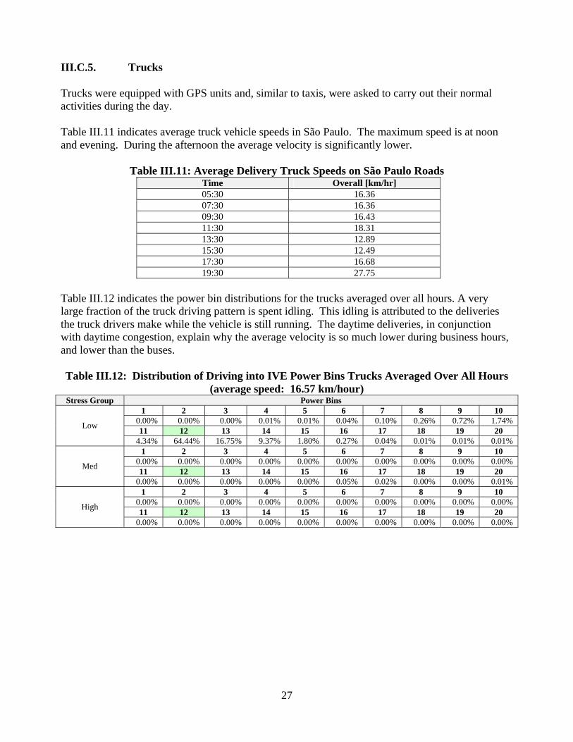
III.C.5. Trucks Trucks were equipped with GPS units and, similar to taxis, were asked to carry out their normal activities during the day. Table III.11 indicates average truck vehicle speeds in São Paulo. The maximum speed is at noon and evening. During the afternoon the average velocity is significantly lower.

Table III.11: Average Delivery Truck Speeds on São Paulo Roads Time Overall [km/hr] 05:30 16.36 07:30 16.36 09:30 16.43 11:30 18.31 13:30 12.89 15:30 12.49 17:30 16.68 19:30 27.75

Table III.12 indicates the power bin distributions for the trucks averaged over all hours. A very large fraction of the truck driving pattern is spent idling. This idling is attributed to the deliveries the truck drivers make while the vehicle is still running. The daytime deliveries, in conjunction with daytime congestion, explain why the average velocity is so much lower during business hours, and lower than the buses. Table III.12: Distribution of Driving into IVE Power Bins Trucks Averaged Over All Hours

(average speed: 16.57 km/hour) Stress Group Power Bins

1 2 3 4 5 6 7 8 9 10 0.00% 0.00% 0.00% 0.01% 0.01% 0.04% 0.10% 0.26% 0.72% 1.74% 11 12 13 14 15 16 17 18 19 20 Low

4.34% 64.44% 16.75% 9.37% 1.80% 0.27% 0.04% 0.01% 0.01% 0.01% 1 2 3 4 5 6 7 8 9 10

0.00% 0.00% 0.00% 0.00% 0.00% 0.00% 0.00% 0.00% 0.00% 0.00% 11 12 13 14 15 16 17 18 19 20 Med

0.00% 0.00% 0.00% 0.00% 0.00% 0.05% 0.02% 0.00% 0.00% 0.01% 1 2 3 4 5 6 7 8 9 10

0.00% 0.00% 0.00% 0.00% 0.00% 0.00% 0.00% 0.00% 0.00% 0.00% 11 12 13 14 15 16 17 18 19 20 High

0.00% 0.00% 0.00% 0.00% 0.00% 0.00% 0.00% 0.00% 0.00% 0.00%

27

III.C.6. Summary of Driving Pattern Results Figure III.6 compares driving speeds by hour for the four types of vehicles studied. In general, congestion lowers the average velocity during the daytime hours by 30 to 60 percent of free flow velocities. It was assumed that the early morning and late evening velocities were similar to the late evening and 6 AM data because no data was collected between 10 pm and 5 AM. Overall, various road types and vehicle types have similar average velocities. It is interesting that the fastest and lowest velocities occur on the highways, the highest speeds during the very early morning hours and lowest velocities in the middle of the day, when average speeds are even lower than on residential roadways. Delivery trucks maintain a relatively low average velocity throughout the day due to the idle time during deliveries. Buses and Motorcycles have similar average speeds to passenger vehicles traveling on arterial and residential roadways.

0

10

20

30

40

50

60

0:00

1:00

2:00

3:00

4:00

5:00

6:00

7:00

8:00

9:00

10:00

11:00

12:00

13:00

14:00

15:00

16:00

17:00

18:00

19:00

20:00

21:00

22:00

23:00

Time of Day (hh:mm)

Ave

rage

Vel

ocity

(kph

)

PCHwy PCRes PCArt 2wHwy 2wRes 2wArt Bus

Figure III.6: Average Speeds for All Road Types and Vehicle Classes in São Paulo

Legend: PC: passenger cars (private cars); 2w: two wheeled vehicles (motorcycles) Hwy: highway; Res: residential; Art: arterial

28

Figure III.7 shows the distribution into driving bins for three of the main classes of driving at 05:30. There is little to distinguish the driving patterns between passenger vehicles, 2-wheel vehicles, and buses at this time of the morning. The 2-wheel vehicles and passenger vehicles are using slightly more relative power (i.e. accelerations) in driving under free flow conditions.

0%

10%

20%

30%

40%

50%

60%

70%

80%

1 3 5 7 9 11 13 15 17 19 21 23 25 27 29 31 33 35 37 39 41 43 45 47 49 51 53 55 57 59

VSP/Stress Bin

Per

cent

of

Driv

ing.

PCHwy PCRes PCArt 2wHwy 2wRes 2wArt Bus

Figure III.7: Comparison of Driving Patterns for Four Major Vehicle Classes for 05:30

Legend: PC: passenger cars (private cars); 2w: two wheeled vehicles (motorcycles) Hwy: highway; Res: residential; Art: arterial

29

Figure III.8 represents driving at 09:30. In this case, the highway passenger vehicles and taxi driving look very similar and contain some higher power driving (bins above 20) which is caused by hard accelerations. The highway driving contains the lowest percentage of idle and low stress driving. All driving patterns are significantly different and contain more idle time than the early morning driving patterns.

0%

10%

20%

30%

40%

50%

60%

1 3 5 7 9 11 13 15 17 19 21 23 25 27 29 31 33 35 37 39 41 43 45 47 49 51 53 55 57 59

VSP/Stress Bin

Per

cent

of

Driv

ing.

PCHwy PCRes PCArt 2wHwy 2wRes 2wArt Bus

Figure III.8: Comparison of Driving Patterns for Four Major Vehicle Classes for 09:30

Legend: PC: passenger cars (private cars); 2w: two wheeled vehicles (motorcycles) Hwy: highway; Res: residential; Art: arterial

30

Figure III.9 represents the 12:30 time frame. This hour of the day represents the most uniform driving among the various vehicle classes. Very little high stress driving is seen here. Both the 09:30 and the 12:30 driving contain much larger proportions of low stress and idle driving.

0%

10%

20%

30%

40%

50%

60%

1 3 5 7 9 11 13 15 17 19 21 23 25 27 29 31 33 35 37 39 41 43 45 47 49 51 53 55 57 59VSP/Stress Bin

Per

cent

of

Driv

ing.

PCHwy PCRes PCArt 2wHwy 2wRes 2wArt Bus

Figure III.9: Comparison of Driving Patterns for Four Major Vehicle Classes for 12:30

Legend: PC: passenger cars (private cars); 2w: two wheeled vehicles (motorcycles) Hwy: highway; Res: residential; Art: arterial

Data sets using the binned data and average speeds are used in the IVE model to correct emission estimates for local driving patterns.

31

32

IV. VEHICLE START PATTERNS IV.A. BACKGROUND AND OBJECTIVES Between10% and 30% of vehicle emissions come from vehicle starts in the United States. This is a significant amount of emissions. Thus, it is important to understand vehicle start patterns in an urban area to fully evaluate vehicle emissions. To measure start patterns, a small device that plugs into the cigarette lighter or otherwise hooks into a vehicles electrical system has been developed. The voltage fluctuations in the electrical system can be used to estimate when a vehicle engine is on and off. This process is described in Appendix A. The main objective of these measurements are to collect a representative sample of the number, time of day, and soak period from passenger vehicles operating in São Paulo. IV.B. METHODOLOGY The vehicle engine start patterns were collected using equipment that senses vehicle system voltage denoted VOCE units. VOCE data can be used to determine when vehicles start, how long they operate, and how long they sit idle between starts. This information is essential to establish vehicle start emissions. The VOCE units were placed in passenger vehicles and left there for a week. Figure IV.1 shows the VOCE setup procedure (left picture), connecting a VOCE unit in the cigarette lighter plug of a passenger car (middle picture), and the download process from the VOCE unit to the computer after completing the data collection at the end of the activity study (left picture).

Figure IV.1: Different stages of the VOCE Data Collection Procedure in São Paulo

IV.C. RESULTS Table IV.1 indicates the measured start and soak patterns for passenger vehicles in São Paulo. Data was successfully collected from 69 passenger vehicles (out of 78 units) over about 6-7 days for each vehicle. This provides about 330 vehicle days of data. The total number of starts per day for the whole group was equal to 6.1 (gross). While this amount of information is significant, it was felt

33

that hour by hour data would include too few events and would thus not be meaningful. Thus, the data was lumped into 2 hour groups.

Table IV.1: Passenger Vehicle Start and Soak Patterns for São Paulo Soak Time

Time frame 15 min 30 min 1 hr 2 hr 3 hr 4 hr 6 hr 8 hr 12 hr +18 hr Overall

24:00-01:59 0.95% 0.11% 0.32% 0.48% 0.37% 0.05% 0.11% 0.21% 0.05% 0.16% 2.80% 02:00-03:59 0.60% 0.25% 0.25% 0.35% 0.25% 0.10% 0.10% 0.05% 0.10% 0.15% 2.20% 04:00-05:59 0.35% 0.00% 0.15% 0.15% 0.05% 0.00% 0.05% 0.30% 0.30% 0.45% 1.80% 06:00-7:59 1.68% 0.41% 0.26% 0.05% 0.15% 0.00% 0.10% 0.56% 2.24% 2.14% 7.60% 08:00-09:59 2.44% 0.56% 0.82% 0.82% 0.26% 0.05% 0.10% 0.31% 1.53% 1.73% 8.60% 10:00-11:59 5.30% 1.43% 1.38% 1.38% 0.77% 0.15% 0.15% 0.10% 0.61% 1.48% 12.80% 12:00-13:59 4.58% 1.54% 2.06% 1.50% 0.83% 0.42% 0.87% 0.20% 0.36% 1.03% 13.40% 14:00-15:59 3.02% 1.08% 1.64% 1.69% 0.87% 0.46% 0.26% 0.20% 0.31% 0.66% 10.20% 16:00-17:59 3.62% 1.68% 1.64% 1.48% 0.91% 0.66% 0.66% 0.25% 1.83% 0.46% 13.20% 18:00-19:59 3.38% 1.17% 1.33% 2.45% 0.77% 0.41% 0.87% 0.15% 0.56% 0.51% 11.60% 20:00-21:59 2.34% 1.02% 1.02% 1.02% 1.06% 0.81% 0.61% 0.05% 0.35% 0.51% 8.80% 22:00-23:59 1.73% 0.66% 0.51% 0.91% 0.46% 1.02% 0.56% 0.05% 0.25% 0.46% 6.60%

Overall 29.99% 9.91% 11.38% 12.28% 6.74% 4.12% 4.44% 2.45% 8.50% 9.75% 100%

The data included in Table IV.1 is shown in Figure IV.1 below, where red columns are hot starts (less than 15 minutes soak time), blue columns represent cold starts (more than 6 hours soak time), and the height of each column indicates the fraction of starts during the different time frames.

0%

2%

4%

6%

8%

10%

12%

14%

0-1 2-3 4-5 6-7 8-910

-1112

-1314

-1516

-1718

-1920

-2122

-23

Time frame [hr]

Frac

tion

of v

ehic

le s

tarts

and

soak

tim

es

+6 hr (cold start)4 hr3 hr2 hr1 hr30 min15 min (hot start)

Figure IV.1: Fraction of Vehicle Starts and Soak Time Distribution in São Paulo

As mentioned earlier, São Paulo passenger vehicles were started 6.1 times per day. This is typical of what is observed in other urban areas that have been studied. Starts per day vary from 6 to 8 for passenger vehicles in the urban areas studied to date. In São Paulo, most starts occur in the 10:00-13:59 time frame. The second highest number of starts is in the 16:00-17:59 period, and the third in

34

the 18:00-19:59 time frame. The highest fraction of cold starts (after 6 or more hours soak time, shown above in blue) occurs in the early morning time frame as would be expected (06:00-09:59), and they are also important during the period from 16:00 to 17:59 hours. These long soak times leave the engine cold and result in much greater start emissions. The higher fraction of hot starts (less than 15 minutes soak time, columns in red) occurs during 10:00 to 13:59 hours. Overall, the number of starts with less than 15 minutes soak time represents 30% of the sample, followed by 12% for 2 hours soak time and 11% for 1 hour soak time (see Table IV.1). Adding together the cold starts from bins 6, 8, 10, 12 and +18 hours, then this group represents 25% of the total number of starts from the whole sample.

35

36

V. IVE APPLICATION AND EMISSIONS RESULTS In order to make estimates of total emissions in Sao Paulo, the total driving in the city must be known. Unfortunately such a measurement is not presently made in Sao Paulo. Thus, other less accurate approaches must be taken. Since this study measured both Passenger Car Driving Per Day and the Fraction of Passenger Cars on the Street, a semi-independent estimate of emissions can be made as follows: Total Passenger Car Driving Per Day = Number Passenger Cars * Passenger Car Driving Per Day Fraction of Passenger Cars on the Street = Total Passenger Car Driving per Day / Total Driving Per Day Thus, Total Driving Per Day = Total Passenger Car Driving Per Day / Fraction of Passenger Cars on Street. Since this study measured the Passenger Car Driving Per Day and the Fraction of Passenger Cars on the Street. The remaining data point needed to estimate total VKT is the Number of Passenger Cars in the region. The government maintains a registration of passenger vehicles in the region, but does not have a mechanism for removing vehicles that are retired from the fleet. Thus, this number exaggerates the number of vehicles. In spite of this problem, the local inventory has been historically developed using this number, which is 5,886,003. According to this registration data base, about 34% of the vehicles in Sao Paulo are 1990 or older. According to the data collected in this study, 10% of the vehicles in Sao Paulo are 1990 or older. Thus, the registration data base should be reduced by 27% to estimate the actual number of vehicles on the street. However, in order to compare estimates in this study with the CETESB developed numbers, the full number in the registration data base will be used. The final indicated emission rates should be reduced by 27% to account for this overestimation. Using the previously discussed process, the estimated daily driving is 356,000,000 (or 261,000,000 if reduced by cars estimated to be retired). The fraction of driving per hour can be estimated using traffic counts shown in Table II.1 and averaged according to the fraction of driving on each type of street discussed in Section II.A. Based on the observed number of vehicles on the different road types and the total length of each type of road in São Paulo, it was estimated that 29.1% of overall driving in São Paulo is on arterials, 4.5% on highways, and 66.4% on residential streets. The results are shown in Table V.1. Since no data was collected between 0:00 and 06:00 and between 21:00 and 0:00 these values were estimated using fractions observed in other urban areas. In the case of vehicle starts, Tables IV.1 and IV.2 were weighted by the fraction of passenger vehicles.

37

Table V.1: Estimated Fraction and VMT and Starts by Hour in São Paulo

Time of Day

Estimated Driving

Fractions in Each Hour

Total Estimated Driving by

Hour (kilometers)

Fraction of Starts in

Each Hour

Total Estimated Starts by

Hour 0:00 0.6% 1937636 0.3% 152777 1:00 0.3% 1004969 0.3% 152777 2:00 0.1% 445368 0.3% 152777 3:00 0.1% 258834 0.3% 152777 4:00 0.1% 258834 0.3% 152777 5:00 0.3% 1004969 1.1% 476524 6:00 1.1% 3802972 1.1% 476524 7:00 5.4% 19014858 1.1% 476524 8:00 7.4% 26034052 8.6% 3849142 9:00 6.6% 23397449 8.6% 3849142

10:00 6.1% 21498088 8.6% 3849142 11:00 6.9% 24401819 7.2% 3210463 12:00 7.0% 24517172 7.2% 3210463 13:00 6.3% 22135397 7.2% 3210463 14:00 6.3% 22217967 6.4% 2861495 15:00 6.4% 22433602 6.4% 2861495 16:00 7.4% 25894316 6.4% 2861495 17:00 7.3% 25547296 6.8% 3019651 18:00 7.1% 25017644 6.8% 3019651 19:00 5.2% 18421269 6.8% 3019651 20:00 4.9% 17406460 2.6% 1168557 21:00 4.0% 13974017 2.6% 1168557 22:00 2.5% 8750844 2.6% 1168557 23:00 0.8% 2702695 0.3% 152777 Total 100% 352078526 100% 44674172

The calculations shown above are for illustrative purposes only. They are approximations and more extensive measurements should be completed in São Paulo to improve the estimate of total daily driving in São Paulo and hourly driving outside of the hours measured in this study.

38

V.A. CARBON MONOXIDE Figure V.1 shows the modeling results using the data developed or estimated from this study for Carbon Monoxide. The top line reflects start and running emissions added together.

0

100

200

300

400

500

600

700

0 1 2 3 4 5 6 7 8 9 10 11 12 13 14 15 16 17 18 19 20 21 22 23

Hour of Day

Emis

sion

s (to

ns/h

our)

RunningStart

Figure V.1: Overall São Paulo Carbon Monoxide Emissions

The morning peak CO emissions are occurring around 07:30 and 09:00 and there is another peak between 15:00 and 18:00 hrs. The minimum during the day occurs around 10:00. Emissions are very low from 21:00 to 04:00. It is also valuable to note the importance of start emissions in São Paulo. Most of the time, they represent almost one third of vehicle CO emissions. Overall, Figure V.1 reflects a total of 8214.9 metric tons of CO emitted per day into the air over São Paulo or an overall daily average emission rate of 23.3 grams/kilometer traveled including starting and running emissions.

39

V.B. VOLATILE ORGANIC COMPOUNDS Figure V.2 shows the modeling results using the data developed or estimated from this study for volatile organic compounds (VOC) including evaporative emissions. The top line reflects start, running, and evaporative emissions added together.

0.0

10.0

20.0

30.0

40.0

50.0

60.0

70.0

80.0

0 1 2 3 4 5 6 7 8 9 10 11 12 13 14 15 16 17 18 19 20 21 22 23

Hour of Day

Emis

sion

s (to

ns/h

our)

Evaporative

Running

Start

Figure V.2: Overall São Paulo Volatile Organic Emissions

There are two VOC peak emissions, one occurring in the morning, which could facilitate ozone formation. Start emissions are not as great a percentage of emissions as is the case for CO, but they are still large. Evaporative emissions are somewhat important as well. Figure V.2 reflects a total of 854.6 metric tons per day of VOC emissions going into the air over São Paulo or an overall daily average emission rate of 2.4 grams/kilometer including starting, running, and evaporative emissions.

40

V.C. NITROGEN OXIDES Figure V.3 shows the modeling results using the data developed or estimated from this study for Nitrogen Oxides (NOx). The top line reflects start and running emissions added together. Start emissions are much lower in this case. There is an evening peak of NOx emissions occurring at 19:00 hours. Figure V.3 reflects a total of 1168 metric tons per day of NOx going into the air over São Paulo or an overall daily average emission rate of 3.3 grams/kilometer including starting and running emissions.

0.0

10.0

20.0

30.0

40.0

50.0

60.0

70.0

80.0

90.0

100.0

0 1 2 3 4 5 6 7 8 9 10 11 12 13 14 15 16 17 18 19 20 21 22 23

Hour of Day

Emis

sion

s (to

ns/h

our)

RunningStart

Figure V.3: Overall São Paulo Nitrogen Oxide Emissions

41

V.D. PARTICULATE MATTER Figure V.4 shows the modeling results using the data developed or estimated from this study for Particulate Matter (PM). The top line reflects start and running emissions added together. Start emissions are much lower in this case although still large. Figure V.4 reflects a total of 44.7 metric tons per day of PM going into the air over São Paulo or an overall daily average emission rate of 0.13 grams/kilometer including starting and running emissions.

0.0

0.5

1.0

1.5

2.0

2.5

3.0

3.5

4.0

0 1 2 3 4 5 6 7 8 9 10 11 12 13 14 15 16 17 18 19 20 21 22 23

Hour of Day

Emis

sion

s (to

ns/h

our)

RunningStart

Figure V.4: Overall São Paulo Particulate Matter Emissions

Data on Figures V.1-V.4 was calculated based on a total daily driving of 352 million kilometers. The emission numbers will of course have to be modified if the total kilometers per day measured in São Paulo are greater than 352,078,526.

42

V.E. EMISSIONS CONTRIBUTION BY VEHICLE TYPE To better understand the emissions created from the São Paulo vehicle fleet, it is useful to look at the contribution of each type of vehicle class. For São Paulo, the major vehicle categories include light duty passenger vehicles and trucks (LD), two wheeled vehicles (2w), Motorcycles (Motorcycles), buses (Bus), and trucks (Truck). The fraction of travel from each of these types of vehicles is shown in the last column of Figure V.5. The percent contribution each of these vehicle types to vehicular CO, VOC, NOx, and PM emissions is also shown in Figure V.5. These results indicate the majority of vehicular CO, VOC, and NOx are from buses and passenger cars.

0%

10%

20%

30%

40%

50%

60%

70%

80%

CO VOC NOX PM VMT

PC Taxi Buses Truck 2w

Figure V.5 Emission Contribution of Each Vehicle Type in São Paulo

Clearly, to reduce PM emissions in São Paulo, buses and trucks must be controlled. To reduce NOx, buses, trucks, and passenger vehicles must be further controlled.

43

V.F. EMISSION RATE COMPARISON Another calculation that is of interest is the overall per kilometer emissions of São Paulo vehicles compared to vehicle fleets in cities of other countries. Figure V.6 compares São Paulo with Los Angeles, Santiago, Mexico, Nairobi, and Pune. These locations have a very different profile of vehicle fleet, fuel type, and driving patterns.

0

2

4

6

8

10

12

14

CO/10 VOC NOx PM*10 CO2/40

Emis

sion

Rat

e (g

/km

)

Los Angeles Nairobi Santiago Pune Mexico Sao Paulo Lima

Figure V.6: Comparison of Daily Average Emission Rates in Countries Studied to Date

The São Paulo fleet has the third highest emissions of NOx and PM. Figures V5 and V6 illustrate the possibilities that if emission rates were lowered, significant emissions reductions could be achieved in the São Paulo area.

44

V.G. VEHICLE ANNUAL EMISSIONS COMPARISON A comparison between the results obtained from this Activity Study and the CETESB 2003 Air Quality Report is shown in Figures V.7 and V.8. The results from the IVEM have been converted from tons of pollutant per day into kton per year.3

0

500

1000

1500

2000

2500

3000

kT/y

ear

IVEM 2662 246 277 378 14CETESB 1758 217 391 395 26

CO HC HC+EV NOx PM

Figure V.7: Comparison of annual vehicle emissions between IVEM and CETESB

0%

20%

40%

60%

80%

100%

120%

140%

160%

IVEM 151% 113% 71% 96% 55%CETESB 100% 100% 100% 100% 100%

CO HC HC+EV NOx PM

Figure V.8: Relative comparison of annual vehicle emissions between IVEM and CETESB

3 The calculation considers 329 days/year, estimated from 250 working days at 100% traffic flow, 53 Saturdays at 80% traffic flow, and 62 Sundays plus holidays at 50% traffic flow.

45

The results shown in the above figures are for São Paulo Metropolitan Region. The IVEM results are 51% higher than CETESB for CO and 13% higher for HC without including evaporative emissions. On the other hand, the IVEM is showing lower results than CETESB for HC including evaporative emissions, nitrogen oxides and particle matter (-29%, -4% and -45% respectively). As noted earlier, we believe the estimates in this paper should be further reduced by 27%. The differences obtained between IVEM and CETESB are mainly due to the emissions factors selected for each methodology (generally higher for the IVEM), the fleet distribution and their technology (IVEM uses dynamic data collected from video tape recordings), and the correction factors for both driving patterns and cold starts. Also, the IVEM considers sulfur content in diesel fuel of 800 ppm, resulting in lower PM emissions. The CETESB inventory has much higher numbers of older vehicles than found in the IVE study and a lower emission rate for post 1995 vehicles than found in the IVE study. Thus, the similarities between the two inventories are somewhat coincidental. As noted earlier, the total vehicle activity data for SPMR has been calculated using the total number of vehicles reported by the Street Traffic Department (DETRAN-SP) and the fleet distribution obtained from video tape analysis. This activity can been compared with results done by IPT.4 The total amount of vehicle kilometers (VKT) per day driven by passenger cars in Sao Paulo City was estimated to be 159,766,207 km/day by IPT. The IVE study estimated that passenger cars drive 46 kilometers per day. Using the Street Traffic Department registration data base, the estimated passenger car driving is 271,000 kilometers per day. As noted earlier, the data from the IVE study indicates that the registration data base is overstated by 27%. If this correction is made then the estimated passenger car driving would be 198,000 kilometers. This is still higher than the IPT estimate with a difference of 38%. A more extensive traffic count activity needs to be conducted in Sao Paulo to improve the estimate of total vehicle operations.

4 Institute for Technological Research (Instituto de Pesquisas Tecnológicas), personal communication with Silvio de Andrade Figueiredo.

46

V.H. CONCLUSIONS In conclusion, this study has developed basic data to allow for improved estimates of emissions from the São Paulo fleet. Additional studies are needed to further improve emission estimates in Brazil, but significant planning activities can occur using the data in this report. Our recommendations are as follows:

1. Use the IVE model along with air quality measurements to map out a strategy for improved future air quality, and then seek to improve the air quality management process by further upgrading the São Paulo database.

2. Investigate the variations of the fleet, activity and fuel quality on areas beyond São Paulo if

extrapolations are to be made to the entire metropolitan area.

3. Improve emission factors for in-use vehicles. More emission studies are needed to verify the operating emissions of passenger vehicles, buses and trucks in São Paulo to insure that the best emission factors are being used. This research is being planned for later in 2004 for São Paulo and Mexico City.

4. Improve the estimate of total VMT for the entire São Paulo Metropolitan Region to support

overall emission estimates. 5. Directly measure toxic emissions from these vehicles to better quantify the toxic emission

rates from these sources.

47

48

49

Appendix A

Data Collection Program Used in São Paulo

1 A.

International Vehicle Emissions Model

Field Data Collection Activities

2 A.

3 A.

Table of Contents A.I. Introduction …………………………………………………………………... A6 A.II. Collecting Representative Data ……………………………………………… A7 A.III. On-Road Driving Pattern Collection Using GPS Technology ………………. A11 A.IV. On-Road Vehicle Technology Identification Using Video Cameras ………… A15 A.V. On-Road Vehicle Technology Identification Using Parked Vehicle Surveys ... A17 A.VI. Vehicle Start-Up Patterns by Monitoring Vehicle Voltage …………….…….. A18 A.VII. Research Coordination and Local Support Needs ……………………….…… A20

4 A.

5 A.

A.I. Introduction This paper provides a description of the activities involved in a 2-week cooperative on-road vehicle study carried out in selected international urban areas. This International Vehicle Emissions (IVE) study is designed to efficiently collect important vehicle related data to support development of an accurate estimate of on-road vehicular emissions for the selected urban area. Emissions from on-road vehicles vary considerably depending upon three factors: 1) vehicle type, 2) driving behavior, and 3) local geographic and cSão Paulotic conditions. Vehicle type is defined by the engine air/fuel management technology and engine size, emissions control technology, fuel type, accumulated use and age of the vehicle. Driving behavior can be described by a measured velocity profile of the local driving, the number and distribution of vehicle starts and daily miles traveled. Local conditions that affect vehicle emissions include road grade, fuel quality, ambient temperature, ambient humidity, and altitude of operation. Data collection in this study will help to define vehicle types and driving behavior in the urban area by collecting four types of information as indicted in Table A.1. Table A.1: Types of Data Collection in the IVE Study

Data Collection Method of Data Collection Described in Section

On-Road Driving Patterns GPS Instrumented Passenger, Bus, 2-Wheeler, and 3-Wheeler Vehicles III

Vehicle Technology Distribution

Digital Video Collection and Parking Lot Surveillance IV, V

Vehicle Counts on Selected Streets Digital Video Collection IV

Vehicle start-up patterns VOCE units placed in recruited vehicles VI

The collected data will be formatted so that it is usable in the new International Vehicle Emission Model developed for estimating criteria, toxic, and global warming pollutants from on-road vehicles. The collected data may also be useable for other purposes by the local urban area. Local temperatures, humidity, fuel quality, total vehicular counts, and total driving amounts are not determined as a part of this study. Locally collected data is typically relied upon for these parameters. It may be possible to make a very rough approximation of total vehicle driving from the collected data if the number of vehicles in the urban area is known, but this approximation is subject to considerable error. To make an accurate emission analysis, the total amount of driving in an urban area must be assessed. If key data outside of the scope of this study is not available, then steps should be considered to determine this important data. ISSRC will work with the urban area to suggest ways to make such assessments.

6 A.

A.II. Collecting Representative Data Before the specific study elements are described, it is important to consider the overall data collection process. The IVE study is carried out over a single 2-week study period. Given that there are limited equipment and study personnel, it is not possible to collect a complete data set over an entire urban area. Thus, the study must be designed to collect representative data that can be extrapolated to the full urban area. The IVE study process has been designed with this thought in mind. On-road driving varies by the time of the day, by the day of the week, and by the location in an urban area. To account for this, during the IVE study, data is collected at different times of the day and in different locations within an urban area. This study is not designed to generally capture data on the weekend or very late at night. Thus, the study is primarily applicable to weekday driving and only limited weekend extrapolations and assumptions about traffic flow very late at night can be made. Conducting a weekend study will produce valuable information and should be considered for future research5. It should also be noted that the collected data could be improved in the future by replicating data collection activities to improve statistics, expanding the parts of the city studied, and expanding the times that are studied. Selecting Parts of a City for Study Three representative sections of the city are normally selected for the IVE study. The areas selected should represent the fleet makeup and the general driving taking place in the city. It is recommended that one of the study areas represent a generally lower income area of the city, one of the study areas represent a generally upper income area of the city, and one of the study areas represent a commercial area of the city. The sections representing the upper and lower income areas of the city for study should not be the absolute poorest or richest part of the city. It is better to select areas that are representative of the lower half of the income and the upper half of the income. Normally the urban center is selected as the best commercial area to study. Due to their much greater knowledge of their own city, it is an important role of the local partners for an IVE study to play a primary role in the selection of the three appropriate parts of the urban area to study. ISSRC is amenable to modifications in the recommended study areas due to unique situations that might occur in a particular urban area. For example, there may not be a large enough discernable upper or lower income area. The following criteria should be used as guidelines for selecting adequate sites:

♦Selection of a low income, upper income, and commercial area with a variety of streets

(i.e. residential, freeway, and arterial) in the area.

♦Accessibility to a representative parking lot or on-street parking where up to 150 parked vehicles can be studied within 10 minutes walking of each site selected.

5 In Los Angeles, some of the worst air pollution levels now occur on the weekend. This is due to the modified driving patterns and fleet mix that occurs on weekends compared to weekdays.

7 A.

Selecting Driving Routes for Study Within each of the study areas, different types of streets must be analyzed to gather data representative of all of urban streets. Streets are often classified into three general groupings. The first group represents streets that are major urban connectors and can connect one urban area to another. These streets are typically characterized by the highest traveling speed in free-flow traffic with minimal stops from cross-flow traffic and are commonly referred to as highways or freeways in some cases. The second classification of streets represents streets that connect sections of an urban area. They may connect one section of an urban area with another or may provide an important connection within a section of the urban area. These streets are typically referred to as arterials. The third classification of streets represents the streets that take people to their homes or small commercial sections of an urban area, and are usually one- or two-lane roadways with a relatively lower average speed and frequent intersections. These streets are typically referred to as residential streets. Due to time limitations, only nine street-sections can be effectively studied during the IVE project. The term “street-section” as used in this study can include parts of more than one street, but to simplify data analysis, the streets that are included within a single street-section should all be the same street classification. For example, residential streets should not be mixed with highways in a single street-section. It is important that the nine selected street sections represent each of the important street types in the urban area. The following criteria should be used as guidelines for selecting suitable street- sections:

♦For each of the street-sections, accessibility to a safe and legal location for the camera team to be dropped where 2 cameras & tripods can be set up with a clear view of the nearby traffic (tripods are approximately 0.5 meters in diameter). This location should be within approximately 5 minutes of the driving route. Preferably, the cameras will capture a portion of the driving trace6 being covered by the chase vehicles.

♦Access to the different street types in a part of the city so that the chase vehicle can move

from one street-section type to another within 10 minutes driving time. This insures that time loss in moving from the highway street-section to the residential street section to the arterial street section and back does not require too much lost driving time.

♦A driving trace for each street segment must be defined so that the driver can complete it

in 50 minutes or less under the worst traffic conditions that will be encountered during the study.

In the upper and lower income sections of the city, it is recommended that a highway street-section, an arterial street-section, and a residential street-section be selected in each of the two areas. In the commercial area it is recommended that a highway section and two arterial sections be selected for study. As noted earlier, the defined street-sections do not have to be the same street, although they should be the same classification of street for a street-section grouping. Figure A.1 shows an example of three street-segments designed for an upper-income area in Los Angeles, California.

6 A driving trace is the route followed by the chase vehicles as they drive along one of the selected street-sections.

8 A.

Figure A.1 Example of a Residential, Arterial, and Freeway Street-Segment Selected for a Single Study Area

Designing a set of interconnected arterials or residential streets that ultimately connect to one another to form a circular drive can provide an effective street-section for this study. This circular design is often not possible with highways and the driver may have to drive one way on a highway and then return on that same highway on the other side of the street. During less congested times, it is often possible that a driver can drive the designated street-section more than one time. This is not a problem and simply adds to the database during a time period. As is the case with selecting general areas of the city to study, it is an important role of the local partners to select the nine streets to be studied. ISSRC will review the nine selected street sections and make recommendations as necessary. Times of Data Collection It is also important to collect data at different times of the day to account for traffic congestion and resulting changing flow rates as the day progresses. Testing is carried out normally over a 6 day period for the collection of urban driving patterns and vehicle technology data. Since driving in difficult traffic situations and collecting on-road vehicle technologies are typically very tiring and dirty activities, data collection is held to about 7 hours each day. Since information is typically needed from 06:00 to 20:00 to understand the complete cycle of traffic flow, the driving times are

9 A.

set for 7 hours in the morning on one day of data collection and 7 hours in the evening the next day of data collection. Data collection is normally started at 06:00 and continues until shortly before 13:00 for the morning data collection and starts at 13:00 and goes to shortly before 20:00 for the afternoon data collection. If special circumstances exist in an area where data is desired at earlier or later times, this should be discussed in advance of the study period. Collecting Other Related Data Parking lot data is collected in the same parts of the city where on-road driving and technology data are collected. It is desirable to capture vehicle technologies that exist down to 1% of the fleet. To increase the probability of seeing the types of vehicles that exist at the 1% level and to improve the accuracy of vehicle use data, it is important to collect data on more than 800 randomly selected parked vehicles over the 6-day study period. Generally, it is attempted to collect data on 300 vehicles in each of the three selected sections of the urban area; however, vehicle availability in lower income sections often reduce the total collected data to 800-850 vehicles in the overall study. In the case of the collection of start-up data, individuals are asked to carry small data collection devices in their vehicles. It is important that the individuals selected for this portion of the study should be representative of the general driving population. It would be best to study at least 300 persons, but lack of time and equipment does not allow this large of a study. As discussed later in this paper, it is more efficient to collect data over more days from fewer persons. In all, it is hoped that more than 100 persons will use the units for at least 3 days per person to provide 300 person-days of information.

10 A.

A.III. On-Road Driving Pattern Collection Using GPS Technology Collection of on-road driving pattern data will be conducted on the streets identified by local agencies as discussed in Section II. This data collection will be conducted using combined Global Positioning Satellite (CGPS) modules with microprocessors developed by CE-CERT and GSSR. The unit is placed on a vehicle that drives on predetermined street sections with the flow of traffic. The CGPS module collects information about the location, speed, and altitude on a second by second basis. For areas with large passenger vehicle, bus, 2-wheeler, and/or 3-wheeler populations it is important to collect independent driving pattern data for all of these vehicles since they will likely operate differently. Eight CGPS modules will be provided for the study: three for passenger vehicles, one for a 2-wheeler, and two each for buses and 3-wheelers. An additional two units are brought as backup units. The collection procedure for each type of vehicle is described later in this section. Figure A.2 shows a typical CGPS unit. They weigh about 5.5 kilograms each and can be strapped to the back of a 2-wheeler or placed on the seat of a passenger vehicle. An antenna is required. In the case of 2-wheelers, 3-wheelers, and buses some experimentation may be required to fina a suitable location for the antenna. The antenna is magnetic and will stick to the roof of automobiles easily. In the case of buses with fiberglass roofs, 2-wheelers, and 3-wheelers tape or other attachment means may be necessary. The antenna may be taped to the top of the CGPS box, the bus roof, or may be attached to the helmet of the 2-wheeler operator.

Figure A.2 CGPS Unit

Driving Pattern Collection for Passenger Vehicles and 2-wheelers To collect general passenger vehicle driving patterns, the local partners for the study must arrange for three passenger vehicles and local drivers to drive for eight hours each day for 6 days. In addition, one CGPS unit will be dedicated to the collection of 2-wheeler data7. The local study

7 The decision to collect data from 2-wheelers and 3-wheelers is dependent upon the size fraction of these types of vehicles in the fleet. In the case of studies in the United States and Chile it was determined that 2-wheelers and 3-wheelers were too small of a portion of the fleets to justify the collection of driving pattern data for these vehicles.

11 A.

partners should identify up to six 2-wheelers and drivers to participate in this study8. Figure A.3 shows a passenger vehicle equipped with a GPS module as used in Santiago, Chile. The CGPS units do not require an operator or laptop computer. Thus, only the driver is necessary.

GPS Antenna

Laptop & Recorder

Driver

GPS Antenna

Laptop & Recorder

Driver

GPS Antenna

Laptop & Recorder

Driver

Figure A.3: GPS Instrumented Vehicle in Santiago, Chile

These drivers are asked to operate their vehicles on the nine designated street-sections (see Section II for a discussion of street-sections) over the course of the study. The purpose of the instrumented vehicle is to collect representative data concerning local passenger vehicle driving patterns. To accomplish this, the vehicle is operated on the selected street-sections in accordance with normal traffic at the time they operate. It is important that the drivers duplicate typical driving patterns for the study area. Each day, one of the instrumented vehicles is assigned to a different selected area of the city (see Section II for a discussion of the general test areas of the urban area). The vehicles will operate in their section of the urban area for two days before moving to the next selected area of the city. The first day they will operate their vehicles in the morning timeframe and the second day they will operate their vehicles in the afternoon timeframe. Each vehicle will operate on a selected street-section for 1 hour and then move to another of the selected street-section in a predetermined pattern. Since there are three street sections in an area, after the third section is reached, the driver will return to the first street section and repeat the process until the end of the 7-hour test period. Table III.1 shows the driving circuits for the three passenger vehicles and 2-wheeler. It is important that the drivers adhere strictly to the defined street-section order to insure that all times of the day are covered. The 3 parts of the urban area designated for study are denoted as Area A, Area B, and Area C. The 3 street-sections selected in each area are designated as street-section 1, 2, or 3. Thus the highway street-section in Area A is designated as Street-Section A.1 and similarly for the others.

8 It should be okay to use as few as three 2-wheelers over the course of the study. It is important to get a cross section of 2-wheeler types that represent different engine sizes. The use of 6 2-wheelers will reduce driver fatigue during the course of the study. One 2-wheeler could operate each day through the 6-day study.

12 A.

Table A.2: Passenger Vehicle and 2-Wheeler Driving Circuits Day 1

Start End Passenger Vehicle 1 Passenger Vehicle 2 Passenger Vehicle 3 & 2-wheeler

06:00 07:00 Street-Section A.1 Street-Section B.1 Street-Section C.1 07:00 08:00 Street-Section A.2 Street-Section B.2 Street-Section C.2 08:00 09:00 Street-Section A.3 Street-Section B.3 Street-Section C.3 09:00 10:00 Street-Section A.1 Street-Section B.1 Street-Section C.1 10:00 11:00 Street-Section A.2 Street-Section B.2 Street-Section C.2 11:00 12:00 Street-Section A.3 Street-Section B.3 Street-Section C.3 12:00 13:00 Street-Section A.1 Street-Section B.1 Street-Section C.1

Day 2 13:00 14:00 Street-Section A.1 Street-Section B.1 Street-Section C.1 14:00 15:00 Street-Section A.2 Street-Section B.2 Street-Section C.2 15:00 16:00 Street-Section A.3 Street-Section B.3 Street-Section C.3 16:00 17:00 Street-Section A.1 Street-Section B.1 Street-Section C.1 17:00 18:00 Street-Section A.2 Street-Section B.2 Street-Section C.2 18:00 19:00 Street-Section A.3 Street-Section B.3 Street-Section C.3 19:00 20:00 Street-Section A.1 Street-Section B.1 Street-Section C.1

Day 3 06:00 07:00 Street-Section B.2 Street-Section C.2 Street-Section A.2 07:00 08:00 Street-Section B.3 Street-Section C.3 Street-Section A.3 08:00 09:00 Street-Section B.1 Street-Section C.1 Street-Section A.1 09:00 10:00 Street-Section B.2 Street-Section C.2 Street-Section A.2 10:00 11:00 Street-Section B.3 Street-Section C.3 Street-Section A.3 11:00 12:00 Street-Section B.1 Street-Section C.1 Street-Section A.1 12:00 13:00 Street-Section B.2 Street-Section C.2 Street-Section A.2

Day 4 13:00 14:00 Street-Section B.2 Street-Section C.2 Street-Section A.2 14:00 15:00 Street-Section B.3 Street-Section C.3 Street-Section A.3 15:00 16:00 Street-Section B.1 Street-Section C.1 Street-Section A.1 16:00 17:00 Street-Section B.2 Street-Section C.2 Street-Section A.2 17:00 18:00 Street-Section B.3 Street-Section C.3 Street-Section A.3 18:00 19:00 Street-Section B.1 Street-Section C.1 Street-Section A.1 19:00 20:00 Street-Section B.2 Street-Section C.2 Street-Section A.2

Day 5 06:00 07:00 Street-Section C.3 Street-Section A.3 Street-Section B.3 07:00 08:00 Street-Section C.1 Street-Section A.1 Street-Section B.1 08:00 09:00 Street-Section C.2 Street-Section A.2 Street-Section B.2 09:00 10:00 Street-Section C.3 Street-Section A.3 Street-Section B.3 10:00 11:00 Street-Section C.1 Street-Section A.1 Street-Section B.1 11:00 12:00 Street-Section C.2 Street-Section A.2 Street-Section B.2 12:00 13:00 Street-Section C.3 Street-Section A.3 Street-Section B.3

Day 6 13:00 14:00 Street-Section C.3 Street-Section A.3 Street-Section B.3 14:00 15:00 Street-Section C.1 Street-Section A.1 Street-Section B.1 15:00 16:00 Street-Section C.2 Street-Section A.2 Street-Section B.2 16:00 17:00 Street-Section C.3 Street-Section A.3 Street-Section B.3 17:00 18:00 Street-Section C.1 Street-Section A.1 Street-Section B.1 18:00 19:00 Street-Section C.2 Street-Section A.2 Street-Section B.2 19:00 20:00 Street-Section C.3 Street-Section A.3 Street-Section B.3

13 A.

It is important that the passenger vehicle and 2-wheeler operators keep a record of the times when their driving should not be included in the analysis due to their taking a rest or leaving the study area. It is also important that the drivers note any unusual traffic conditions that would invalidate the data. Each driver is to be supplied with a writing tablet and pen in order to make records of unusual traffic situations. The CGPS unit will record information on where the driver operated the vehicle and how it was operated. Thus, data analysis will indicate if the proper driving routes were followed. Measurement of Bus and 3-Wheeler Driving Patterns In the case of 3-wheelers and buses, student participants will be asked to take passage on suitable buses and 3-wheeler vehicles operating on the street sections of interest. Four units are dedicated to this purpose. Two units will be used for 3-wheelers and two units will be used for buses9. Care should be taken to select likely bus routes and 3-wheeler routes to be used before the study begins in order to avoid lost time once ISSRC personnel reach the study area.

9 The reserve CGPS units could also be used if the local partners are willing to provide additional 2-wheelers or students to collect bus and 3-wheeler data. Of course, if a CGPS unit fails the reserve units will have to be moved to replace the failed unit.

14 A.

A.IV. On-Road Vehicle Technology Identification Using Digital Video Cameras Two digital video cameras are set up on the roadside or above the road to capture images of the vehicles driving by. This data is later manually reviewed to determine the number, size and type of vehicle. It is important to set the cameras at an appropriate height in order to have a good view of traffic on one side of a roadway. Useful data can be captured with the cameras located at the roadside, but on busy roads it is best to have the cameras elevated 1 to 3 meters above the street level when possible. Figure IV.1 shows videotaping in Santiago, Chile on a residential street. In this case due to the low traffic volume and small street size, videotaping could be carried out at street level. Figure A.4 shows videotaping from an overpass of a freeway in Los Angeles, California. In this case due to the high traffic volume and the multiple lane roadways, data is best collected from directly above the street. Data is collected on the same roads and at the same times when driving patterns are being collected. This allows driving speeds and patterns determined from the CGPS units (discussed earlier in this paper) to be correlated with traffic counts taken from the digital video cameras. Thus, selection of roadways, as discussed in Section II, should consider the video taping requirements as well.

Figure A.4: Cameras collecting data on a resident

15 A.

Detail Camera

ial roadway in S

Traffic Count Camera

antiago, Chile

Camera Setup on the Overpass Picture of the Freeway Below

Figure A.5: Camera collecting data from a freeway overpass in Los Angeles, California The digital video cameras and the two operators usually travel with one of the instrumented vehicles to their desired location. Videotapes for analysis are collected for at least 20 minutes out of each hour and preferably for 40 minutes of each hour. Local citizens passing the cameras often have questions and upon occasion, the police become concerned about the operation of the cameras. It is important to provide a local person to explain the purpose of the data collection effort to avoid raising local concerns. It should also be noted that working along side the street for up to 7 hours a day could expose the video taping crew to considerable dust and other pollutants. It is recommended that the camera operators have good quality dust masks for cases where the dust levels are high. Each day about 3.5 hours of videotapes are collected. These videotapes are analyzed the following day by student workers and ISSRC staff to develop the needed data for establishing on-road fleet fractions. ISSRC will provide two videotape readers and laptop computers to support analysis of the data during the data collection process.

16 A.

A.V. On-Road Vehicle Technology Identification Using Parked Vehicle Surveys The on-road technology identification process using digital video cameras does not collect all of the information required to completely identify the vehicle. Therefore, it is important to supplement this data by visual inspection of parked vehicles using on-street and parking lot surveys. Figure V.1 shows data collection in a Nairobi parking lot. By use of an experienced mechanic recruited from the local area, model year distributions, odometer (distance traveled) data, air conditioning, engine air/fuel control, engine size, and emissions control technology can be estimated for the local fleet using this type of survey technique. Studies in Los Angeles indicate that the technology distributions found in parking lots and along the street closely mirror the on-road vehicle fleet.

Figure A.6: Parking Lot Data Collection in Nairobi, Kenya

The determination of the needed data involves looking inside of parked vehicles. This process can alarm vehicle owners and the police upon occasion. It is important that a local person participate in the parking lot survey that can explain the purpose of the study and resolve concerns of local law enforcement officials. Surveys are conducted in the same general areas where the vehicle driving patterns are collected. The parked vehicle survey team typically rides to their daily study area with the second instrumented vehicle (the first instrumented vehicle carries the on-road camera crew). The second instrumented vehicle leaves the parked vehicle survey team at a suitable location where sufficient numbers of parked vehicles can be found. This instrumented vehicle returns at the end of the study to pick up the surveyors. As noted earlier it is desirable to collect data on more than 800 vehicles. Thus, the daily goal for the parking lot survey crew is 150 vehicles.

17 A.

A.VI. Vehicle Start-Up Patterns by Monitoring Vehicle Voltage As noted earlier, vehicles pollute more when they are first started compared to operations when they are fully warmed up. The colder the vehicle when started, the typically greater emissions. It is thus important to know how often vehicles are started in an urban area and how long a vehicle is off between starts to make an accurate estimate of start-up emissions. ISSRC will bring 56 Vehicle Occupancy Characteristics Enumerator (VOCE) units to measure the times that vehicles are started and how often. These VOCE units will also give us information on how long vehicles are typically operated at different hours of the day. Figure VI.1 shows one of the units in a typical application. It is normally plugged into the cigarette lighter in the vehicle and left there for up to a week at a time, collecting data all the while.

Cigarette Lighter Plug

t

Figure A.7: VOCE Unit for Collecting Vehicle Start Informat The VOCE units operate by simply recording vehicle voltage on a second by secovoltage rises when the vehicle is operated. Software has been developed to downldata from the units. In cases where there are no cigarette lighters, clamps are avaiclamp the VOCE units to the vehicle battery or other suitable location to capture During the study, 50 of the VOCE units will be distributed to local vehicle ownertheir vehicles for four days. The units are then retrieved, the data downloaded, an50 different vehicle owners for another four days. To complete this part of the sparticipants must be identified by the local partners to use the units by the titeam reaches the location. The VOCE units are distributed within the first 24 hothe ISSRC team. At the end of 4 days, the units are retrieved, the data downloadethe units re-distributed the next day for another 4 days. This will give us 400 persinformation. In some cases when a weekend intervenes, the units are left for morewith the vehicle owners and weekend data is collected. The VOCE units are capa

18 A.

VOCE Uni

ion

nd basis. The oad and interpret lable to directly system voltage.

s and attached to d given back out to tudy, 100 me the ISSRC urs after arrival of d over night, and on days of than four days

ble of operating

and collecting data for more than a week if necessary. There will be 6 extra VOCE units that can be used to replace units if they become faulty. In past studies, the vehicle owners have installed the units themselves since they normally only have to be plugged into the vehicles cigarette lighter and left there for the four days of data collection. In cases where the vehicle does not have a cigarette lighter, ISSRC personnel and local partners may have to help the vehicle owner to install the unit. It is important that none of the VOCE units are lost because they are each hand built and can not be easily replaced. To complete this part of the operation, one local person is normally required to spend most of their time during the testing program to first identify 100 participants in advance and then to give out and retrieve the units. Vehicle owners often forget to bring the VOCE units back when they are supposed to or have a problem that keeps them from coming to work to return the units. Thus, while simple in concept, identification, deployment and retrieval of 50 units in the proper timeframe can be a complicated and tedious process. Finally, in selecting vehicle owners to use the VOCE units it is import to select persons that represent a cross section of drivers in the urban area of interest.

19 A.

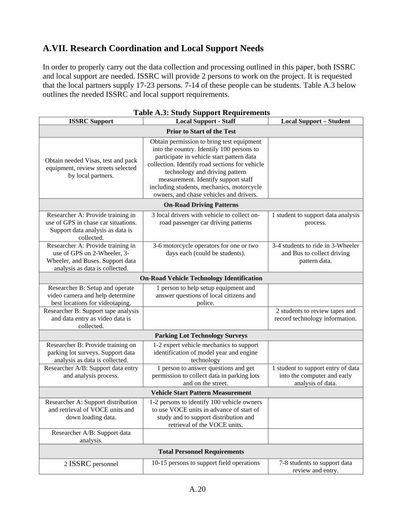
A.VII. Research Coordination and Local Support Needs In order to properly carry out the data collection and processing outlined in this paper, both ISSRC and local support are needed. ISSRC will provide 2 persons to work on the project. It is requested that the local partners supply 17-23 persons. 7-14 of these people can be students. Table A.3 below outlines the needed ISSRC and local support requirements.

Table A.3: Study Support Requirements ISSRC Support Local Support - Staff Local Support – Student

Prior to Start of the Test

Obtain needed Visas, test and pack equipment, review streets selected

by local partners.

Obtain permission to bring test equipment into the country. Identify 100 persons to participate in vehicle start pattern data

collection. Identify road sections for vehicle technology and driving pattern

measurement. Identify support staff including students, mechanics, motorcycle

owners, and chase vehicles and drivers.

On-Road Driving Patterns Researcher A: Provide training in use of GPS in chase car situations.

Support data analysis as data is collected.

3 local drivers with vehicle to collect on-road passenger car driving patterns

1 student to support data analysis process.

Researcher A: Provide training in use of GPS on 2-Wheeler, 3-

Wheeler, and Buses. Support data analysis as data is collected.

3-6 motorcycle operators for one or two days each (could be students).

3-4 students to ride in 3-Wheeler and Bus to collect driving

pattern data.

On-Road Vehicle Technology Identification Researcher B: Setup and operate video camera and help determine

best locations for videotaping.

1 person to help setup equipment and answer questions of local citizens and

police.

Researcher B: Support tape analysis and data entry as video data is

collected.

2 students to review tapes and record technology information.

Parking Lot Technology Surveys Researcher B: Provide training on parking lot surveys. Support data

analysis as data is collected.

1-2 expert vehicle mechanics to support identification of model year and engine

technology

Researcher A/B: Support data entry and analysis process.

1 person to answer questions and get permission to collect data in parking lots

and on the street.

1 student to support entry of data into the computer and early

analysis of data. Vehicle Start Pattern Measurement

Researcher A: Support distribution and retrieval of VOCE units and

down loading data.

1-2 persons to identify 100 vehicle owners to use VOCE units in advance of start of

study and to support distribution and retrieval of the VOCE units.

Researcher A/B: Support data analysis.

Total Personnel Requirements

2 ISSRC personnel 10-15 persons to support field operations 7-8 students to support data review and entry.

20 A.

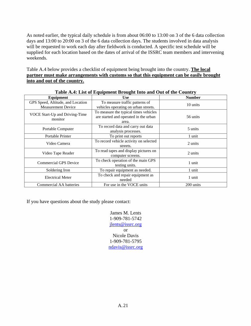
As noted earlier, the typical daily schedule is from about 06:00 to 13:00 on 3 of the 6 data collection days and 13:00 to 20:00 on 3 of the 6 data collection days. The students involved in data analysis will be requested to work each day after fieldwork is conducted. A specific test schedule will be supplied for each location based on the dates of arrival of the ISSRC team members and intervening weekends. Table A.4 below provides a checklist of equipment being brought into the country. The local partner must make arrangements with customs so that this equipment can be easily brought into and out of the country.

Table A.4: List of Equipment Brought Into and Out of the Country Equipment Use Number

GPS Speed, Altitude, and Location Measurement Device

To measure traffic patterns of vehicles operating on urban streets. 10 units

VOCE Start-Up and Driving-Time monitor

To measure the typical times vehicles are started and operated in the urban

area. 56 units

Portable Computer To record data and carry out data analysis processes. 5 units

Portable Printer To print out reports 1 unit

Video Camera To record vehicle activity on selected streets. 2 units

Video Tape Reader To read tapes and display pictures on computer screens. 2 units

Commercial GPS Device To check operation of the main GPS testing units. 1 unit

Soldering Iron To repair equipment as needed. 1 unit

Electrical Meter To check and repair equipment as needed 1 unit

Commercial AA batteries For use in the VOCE units 200 units

If you have questions about the study please contact:

James M. Lents 1-909-781-5742 jlents@issrc.org

or Nicole Davis

1-909-781-5795 ndavis@issrc.org

21 A.

Example of the Work Schedule for Pune India

March 2,2003 March 3, 2003 March 4, 2003

March 5, 2003 March 6, 2003

March 7, 2003 March 8, 2003

Sunday Monday Tuesday Wednesday Thursday Friday Saturday Depart Los

Angeles for Mumbai, India

Arrive Mumbai, India at

23:35 and spend the night in

Mumbai. March 9,

2003 March 10,

2003 March 11,

2003 March 12,

2003 March 13,

2003 March 14,

2003 March 15,

2003 Sunday Monday Tuesday Wednesday Thursday Friday Saturday

Picked up by van at 12:30

and transported

from Mumbai to Pune

Meet with Pune study

group at about 10:00 to

discuss study and use of equipment. VOCE units distributed to

first 50 participants.

1st day of on-road testing, video taping, and parking lot surveys.

2nd day of on-road testing, video taping, and parking lot surveys. Begin processing collected data.

3rd day of on-road testing, video taping, and parking lot surveys.

Process collected

data.

4th day of on-road testing, video taping,

and parking lot surveys. Process

collected data.

March 16, 2003

March 17, 2003

March 18, 2003

March 19, 2003

March 20, 2003

March 21, 2003

March 22, 2003

Sunday Monday Tuesday Wednesday Thursday Friday Saturday No field data

collection or processing.

First 50 VOCE Units

collected. Data downloaded in

the evening.

5th day of on-road testing, video taping, and parking lot surveys.

VOCE Units distributed to

2nd 50 participants as early in day as

possible. Process

collected data.

6th day of on-road testing, video taping, and parking lot surveys. Process collected data.

Process collected

data.

2nd 50 VOCE units collected

and data downloaded. Meet at about

10:00 to review data collected

and preliminary

results of the study. Depart

by van for airport in

Mumbai at about 5PM.

Depart Mumbai at

01:05 Saturday morning.

22 A.

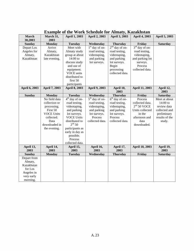
Example of the Work Schedule for Almaty, Kazakhstan March 30,2003

March 31, 2003

April 1, 2003 April 2, 2003 April 3, 2003 April 4, 2003 April 5, 2003

Sunday Monday Tuesday Wednesday Thursday Friday Saturday Depart Los Angeles for

Almaty, Kazakhstan

Arrive Almaty,

Kazakhstan late evening.

Meet with Almaty study group at about

14:00 to discuss study

and use of equipment. VOCE units distributed to

first 50 participants

1st day of on-road testing, videotaping, and parking lot surveys.

2nd day of on-road testing, videotaping, and parking lot surveys. Begin processing collected data.

3rd day of on-road testing, videotaping,

and parking lot surveys. Process

collected data.

April 6, 2003 April 7, 2003 April 8, 2003 April 9, 2003 April 10, 2003

April 11, 2003 April 12, 2003

Sunday Monday Tuesday Wednesday Thursday Friday Saturday No field data

collection or processing.

First 50 VOCE Units

collected. Data

downloaded in the evening.

4th day of on-road testing, videotaping, and parking lot surveys.

VOCE Units distributed to

2nd 50 participants as early in day as

possible. Process

collected data.

5th day of on-road testing, videotaping, and parking lot surveys.

Process collected data.

6th day of on-road testing, videotaping, and parking lot surveys. Process collected data.

Process collected data. 2nd 50 VOCE

Units collected in the

afternoon and data

downloaded.

Meet at about 14:00 to

review data collected and preliminary

results of the study.

April 13, 2003

April 14, 2003

April 15, 2003

April 16, 2003

April 17, 2003

April 18, 2003 April 19, 2003

Sunday Monday Tuesday Wednesday Thursday Friday Saturday Depart from

Almaty, Kazakhstan

for Los Angeles in very early morning.

23 A.

24 A.

Appendix B

Estudo de Atividade de Fontes Móveis na RMSP

B.1

B.2

Estudo de Atividade de Fontes Móveis na RMSP – 12 a 23 de Abril de 2004

O International Sustainable Systems Research – ISSRC, representado pelos Drs. Jim Lents, Nick Nikkila e Mauricio Osses foi contratado pela Fundação Hewlett para elaborar o inventário de emissões de fontes móveis na Região Metropolitana de São Paulo - RMSP, por meio da aplicação do International Vehicle Emissions Model – IVE (http://www.gssr.net/ive/index.html). Os trabalhos de coleta de dados na RMSP foram realizados de 12 a 23 de abril de 2004. O IVE também foi aplicado recentemente em Los Angeles, México, Santiago, Lima, Pune, Almaty e em breve, será levado a Xangai e Pequim.

O modelo se baseia na atribuição de fatores de emissão básicos (em g/km) às diferentes tecnologias de motorização (carburador, injeção eletrônica, catalisador etc) e regimes de operação (carga no motor, temperatura ambiente, velocidade e aquecimento do catalisador) ajustados por fatores de correção relacionados às características locais do combustível (teor de enxofre), e ao estado de manutenção da frota (com ou sem programa de inspeção veicular). Além dos poluentes veiculares convencionais, são estimadas as emissões de poluentes tóxicos, e ainda, de gases do efeito estufa, incluindo: CO, COV’s, NOx, PM2.5, PM10, N2O, CH4, NH3, Benzeno, 1,3 butadieno, aldeídos e CO2.

As duas semanas dedicadas à coleta de dados consistiram de quatro atividades básicas, necessárias à caracterização da atividade veicular na RMSP:

(1) Três veículos leves de aluguel, diversos ônibus urbanos, 12 caminhões, uma motocicleta e dois táxis foram equipados com GPS durante 6 dias úteis. Os GPS eram recolhidos ao final da jornada diária para recarga e download dos dados de posição, velocidade e altitude, segundo a segundo. A partir desses dados, o modelo estima a carga imprimida ao motor a cada instante. Para os veículos leves, foram escolhidos três percursos para cada uma de três áreas da cidade com características distintas: baixo (Campo Limpo/Capão Redondo) e alto (Alto de Pinheiros) poder aquisitivo, e comercial central (23 de Maio/Jardins). Os percursos consistem de três sub-trechos correspondentes a vias expressas, arteriais e residenciais, visando melhor representar os deslocamentos reais realizados na cidade. Em três dias, eles circularam das 7 às 14 h e nos demais, das 14 às 21h, para cobrir o período em que ocorrem a maior parte das viagens. Nos ônibus, dois estagiários, cada um em um ônibus diferente, circularam durante sete horas diariamente munidos de GPS. Com a colaboração de empresas de transporte de carga, 12 caminhões de entrega (2 por dia) foram escolhidos. Um estagiário instalava e recolhia os GPS ao final da jornada. Da mesma forma, uma motocicleta selecionada entre empresas de entregas rápidas e dois Motorcycles circularam em seus percursos de rotina munidos de GPS.

(2) Uma pesquisa sobre a composição tecnológica da frota em estacionamentos de áreas próximas aos percursos dos veículos leves foi realizada durante os 6 dias de atividade. Dois mecânicos experientes e duas estagiárias de relações públicas pesquisaram 1427 veículos quanto à marcação do odômetro, existência de ar condicionado, capacidade do motor e tipo de equipamento de controle de emissões.

(3) A composição básica do tráfego (número de veículos de passageiros, táxis, motos, caminhões leves e pesados, peruas, e ônibus) foi registrada com duas câmeras de vídeo operando simultaneamente nas diferentes áreas, durante os 6 dias úteis, por 7 horas/dia. Um operador de câmera e um auxiliar realizaram os trabalhos de campo. Dois estagiários faziam diariamente a contagem mediante a leitura dos vídeos.

B.3

(4) Monitoramento do regime de partidas em veículos de 80 voluntários previamente selecionados pela SMA/CETESB. A seleção dos voluntários tentou seguir o mais fielmente possível o espectro de operação da frota circulante de veículos leves da RMSP. Os monitores de partida fornecidos foram conectados ao acendedor de cigarros dos veículos na quinta-feira da primeira semana e recolhidos na quinta-feira da semana seguinte. Após sua devolução, foi feita a leitura dos registros de horário de cada acionamento e desligamento do motor. Dessas informações, o modelo calcula o tempo das viagens e a duração da operação com o motor/catalisador frio – com reflexo direto nos fatores de emissão selecionados pelo modelo.

Ainda resta à CETESB levantar o perfil tecnológico da frota a diesel (ônibus e caminhões) numa amostra de 500 veículos observados, a partir da placa de identificação e consulta ao cadastro do DETRAN. Ao ISSRC, caberá o processamento no IVE dos dados coletados e a emissão do relatório final. O Dr. Jim Lents sinalizou para a realização de uma apresentação dos resultados em agosto do corrente.

A segunda etapa dos trabalhos do ISSRC deve ocorrer no segundo semestre, quando uma amostra de veículos será equipada com medidores de gases a bordo e serão levantados os fatores de emissão necessários à calibração do modelo.

Elaborado por: Eng. Olimpio – CTc-A – 30.04.04

B.4