Embed Size (px)
Citation preview

Beijing Vehicle Activity Study
Conducted May 24 – June 4, 2004 Final Report Submitted January, 2005
Liu Huan, [email protected] University of Tsinghua (http://www.tsinghua.edu.cn) Department of Environmental Science & Engineering
Tsinghua, Beijing, 100084, China He Chunyu, [email protected]
Beijing Technology and Business University (http://www.btbu.edu.cn)The college of Chemistry and Environment Engineering
BTBU, Beijing, China James Lents, [email protected] Nicole Davis, [email protected]
International Sustainable Systems Research (http://www.issrc.org) 21573 Ambushers St., Diamond Bar, CA 91765, USA
Mauricio Osses, [email protected] University of Chile (http://www.uchile.cl)
Department of Mechanical Engineering, Casilla 2777, Santiago, Chile Nick Nikkila, [email protected]
Global Sustainable Systems Research (http://www.gssr.net/) 7146 Aloe Court, Rancho Cucamonga, CA 91739, USA

ii

Table of Contents
EXECUTIVE SUMMARY
I. INTRODUCTION................................................................................................................................................... 5 II. VEHICLE TECHNOLOGY DISTRIBUTION.................................................................................................... 6
II.A. BACKGROUND AND OBJECTIVES ...................................................................................................................... 6 II.B. METHODOLOGY ............................................................................................................................................... 6 II.C. SURVEY RESULTS........................................................................................................................................... 11
II.C.1. Fleet Composition................................................................................................................................ 11 II.C.2. Passenger Vehicle Technology Distribution........................................................................................ 13 II.C.3. Passenger Vehicle Use......................................................................................................................... 16 II.C.4. Taxi Vehicle Technology Distribution ................................................................................................. 18 II.C.5. Bus Vehicle Technology Distribution .................................................................................................. 20 II.C.6. Truck Vehicle Technology Distribution ............................................................................................... 21
III. VEHICLE DRIVING PATTERNS ................................................................................................................ 23 III.A. BACKGROUND AND OBJECTIVES..................................................................................................................... 23 III.B. METHODOLOGY ............................................................................................................................................. 23 III.C. RESULTS ........................................................................................................................................................ 26
III.C.1. Passenger Cars .................................................................................................................................... 26 III.C.2. Taxis..................................................................................................................................................... 29 III.C.3. Buses .................................................................................................................................................... 30 III.C.4. Trucks .................................................................................................................................................. 31 III.C.5. Summary of Driving Pattern Results ................................................................................................... 32
IV. VEHICLE START PATTERNS..................................................................................................................... 36 IV.A. BACGROUND AND OBJECTIVES ....................................................................................................................... 36 IV.B. METHODOLOGY ............................................................................................................................................. 36 IV.C. RESULTS ......................................................................................................................................................... 36
V. IVE APPLICATION AND EMISSIONS RESULTS......................................................................................... 38 APPENDIX A DATA COLLECTION PROGRAM USED IN BEIJING............................................... A.1 APPENDIX B DAILY LOG OF THE DATA COLLECTION PROGRAM CONDUCTED IN BEIJING B.1
iii
EXECUTIVE SUMMARY Beijing, China was visited from May 23, 2004 to June 4, 2004 to collect and analyze data related to on-road transportation. The study effort was designed to support estimates of the air pollution impacts of on-road transportation in Beijing that will be used in the development of air quality management plans for the region. It is also hoped that the collected data can be extrapolated to other Chinese cities to support environmental improvement efforts in the other cities as well. The data collection effort was a partnership between Tsinghua University, Beijing Technology and Business University, and the International Sustainable Systems Research Center (ISSRC) in cooperation with the University of California at Riverside (UCR). The ISSRC provided technical support while the Energy Foundation of USA provided financial support. In all, about thirty persons participated in data collection activities over an approximate two weeks period. The study collected three types of information important to the estimation of emissions on vehicles operating on Beijing streets: technology distribution, driving patterns, and start patterns. Each area is summarized below. Vehicle Technology Distribution
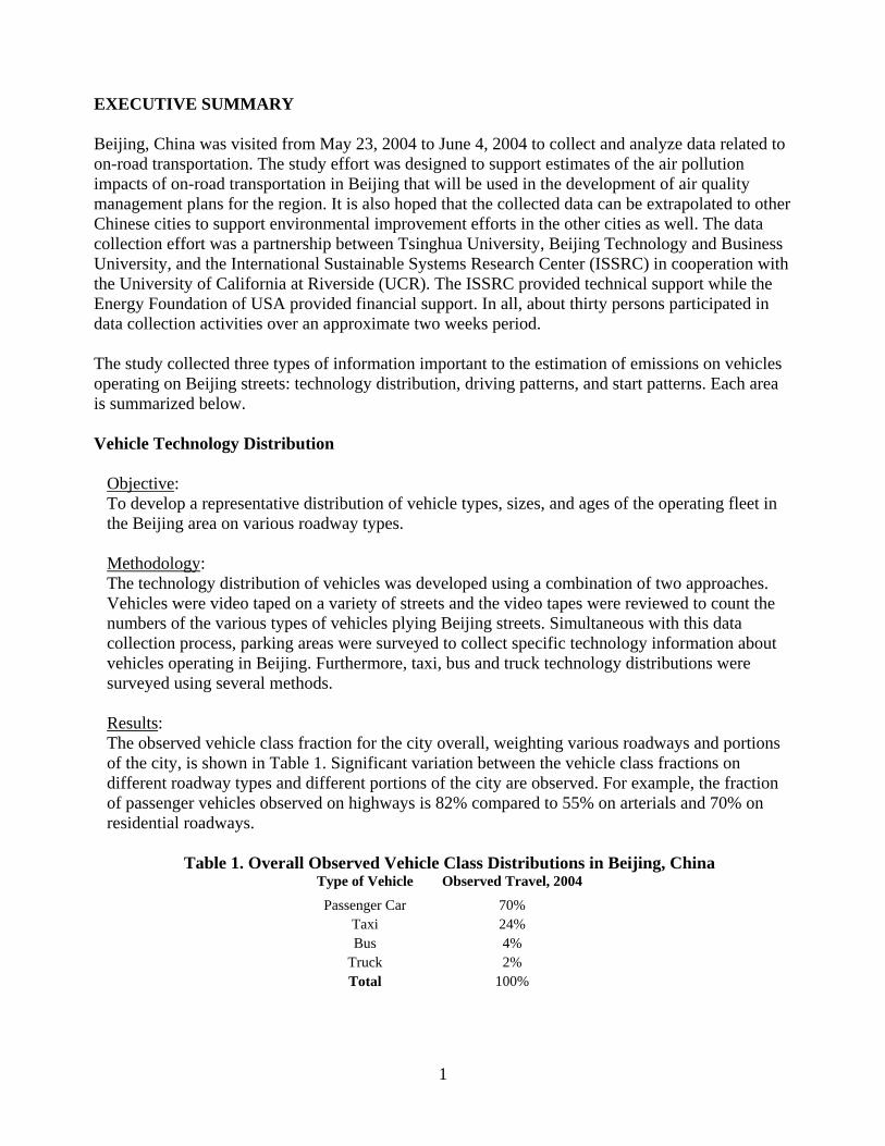
Objective: To develop a representative distribution of vehicle types, sizes, and ages of the operating fleet in the Beijing area on various roadway types. Methodology: The technology distribution of vehicles was developed using a combination of two approaches. Vehicles were video taped on a variety of streets and the video tapes were reviewed to count the numbers of the various types of vehicles plying Beijing streets. Simultaneous with this data collection process, parking areas were surveyed to collect specific technology information about vehicles operating in Beijing. Furthermore, taxi, bus and truck technology distributions were surveyed using several methods. Results: The observed vehicle class fraction for the city overall, weighting various roadways and portions of the city, is shown in Table 1. Significant variation between the vehicle class fractions on different roadway types and different portions of the city are observed. For example, the fraction of passenger vehicles observed on highways is 82% compared to 55% on arterials and 70% on residential roadways.
Table 1. Overall Observed Vehicle Class Distributions in Beijing, China Type of Vehicle Observed Travel, 2004
Passenger Car 70% Taxi 24% Bus 4%
Truck 2% Total 100%
1
In addition to observing the class distribution, a separate survey was conducted to determine the emissions control technology and engine type of the passenger fleet. Approximately 90% have three way catalysts. The majority of passenger vehicles on the road are gasoline multipoint fuel injection vehicles are less than four years old. Vehicle Driving Patterns
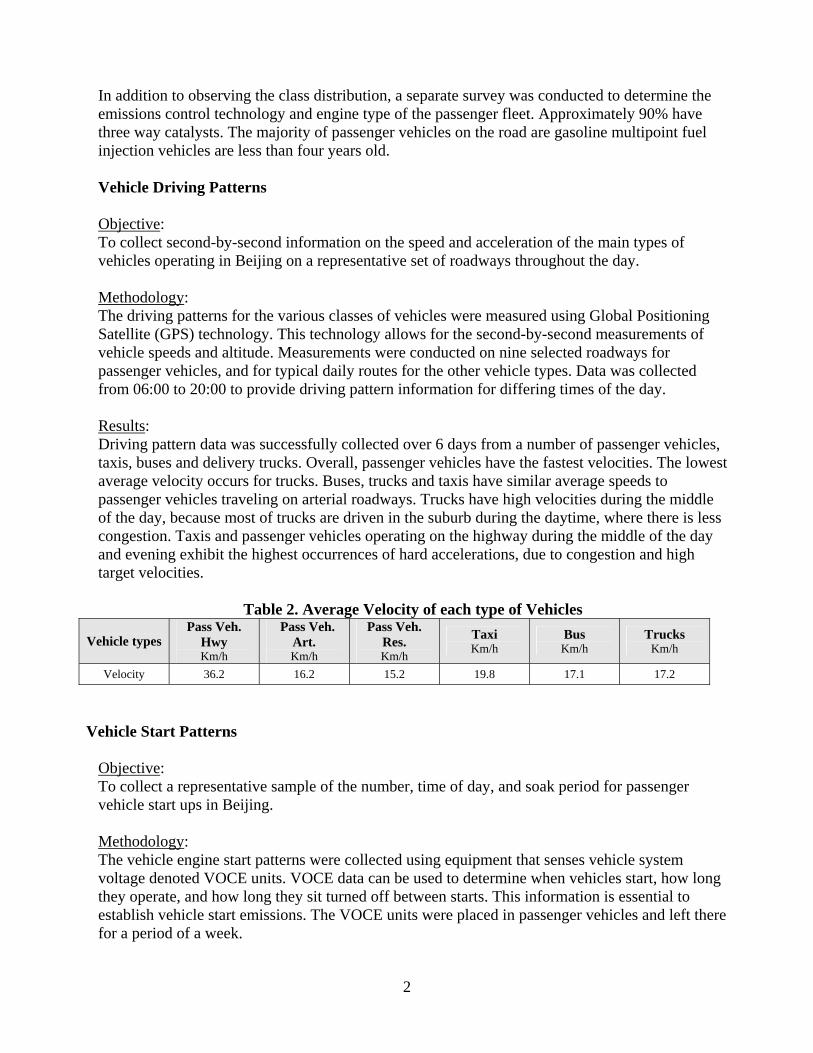
Objective: To collect second-by-second information on the speed and acceleration of the main types of vehicles operating in Beijing on a representative set of roadways throughout the day. Methodology: The driving patterns for the various classes of vehicles were measured using Global Positioning Satellite (GPS) technology. This technology allows for the second-by-second measurements of vehicle speeds and altitude. Measurements were conducted on nine selected roadways for passenger vehicles, and for typical daily routes for the other vehicle types. Data was collected from 06:00 to 20:00 to provide driving pattern information for differing times of the day. Results: Driving pattern data was successfully collected over 6 days from a number of passenger vehicles, taxis, buses and delivery trucks. Overall, passenger vehicles have the fastest velocities. The lowest average velocity occurs for trucks. Buses, trucks and taxis have similar average speeds to passenger vehicles traveling on arterial roadways. Trucks have high velocities during the middle of the day, because most of trucks are driven in the suburb during the daytime, where there is less congestion. Taxis and passenger vehicles operating on the highway during the middle of the day and evening exhibit the highest occurrences of hard accelerations, due to congestion and high target velocities.
Table 2. Average Velocity of each type of Vehicles
Vehicle types Pass Veh.
Hwy Km/h
Pass Veh. Art. Km/h
Pass Veh. Res. Km/h
Taxi Km/h
Bus Km/h
Trucks Km/h
Velocity 36.2 16.2 15.2 19.8 17.1 17.2
Vehicle Start Patterns
Objective: To collect a representative sample of the number, time of day, and soak period for passenger vehicle start ups in Beijing. Methodology: The vehicle engine start patterns were collected using equipment that senses vehicle system voltage denoted VOCE units. VOCE data can be used to determine when vehicles start, how long they operate, and how long they sit turned off between starts. This information is essential to establish vehicle start emissions. The VOCE units were placed in passenger vehicles and left there for a period of a week.
2

Results: Over 630 days of start patterns from 75 different vehicles were collected during the study period. The VOCE units failed for a variety of reasons in 28% of the vehicles. The results show that on average, a typical passenger car is started 6.7 times per day. Approximately 25% of the starts occur between 6 am and 9 am, and another 25% occur between 2 pm and 5 pm. In the early morning hours, over half of the starts occur after having soaked over 12 hours. These long soaks leave the engine cold, which results in increased starting emissions.
Conclusions
The three types of data collected in this study have been used to compile a comprehensive analysis of the make-up and behavior of the current on-road mobile fleet in Beijing. This data is pertinent for correctly estimating current mobile source emissions and projecting the impact of proposed control strategies and growth scenarios, because the vehicle type, speed profiles, and the number of starts and the soak period have a large impact on the mobile source emissions inventory. The data collected in this study was formatted to allow vehicle emissions estimates using the International Vehicle Emissions Model (http://www.issrc.org/ive or www.gssr.net/ive). The IVE model was developed with USEPA funding to make emissions estimates under different technology and driving situations as found in various countries, and has been used extensively in several developing countries. Although up-to date vehicles activity and fleet information was collected in this study, no emissions measurements were made. All emission estimates conducted using the IVE model’s default emission rates. It is recommended that some emission measurements be conducted to create Beijing specific emissions. Of all the areas observed to date, Beijing has the lowest percentage of trucks. That is because trucks are not allowed to drive on the streets inside of the circle 4 road between the hours of 7 am and 9 pm. Also Beijing has the highest percentage of taxis. Beijing’s passenger fleet is comprised of approximately 10% non catalyst vehicles, compared to 1% in the US; 20-30% in Mexico City, Santiago, and Pune; and 90-100% in Almaty and Nairobi. A preliminary emissions analysis using the IVE model indicates that on the order of 2.5 metric tons of PM, 198.6 tons of NOx, 192 tons of VOC, and 2402.5 tons of CO are emitted from on-road motor vehicles each day in Beijing. By viewing the contribution of various vehicle types to the inventory, it was determined that to reduce PM (and toxic) emissions in Beijing, buses and trucks must be controlled. To reduce NOx, CO, VOC, CO2, passenger vehicles must be further controlled. The Beijing fleet has the third highest CO2 emissions (per kilometer) and the lowest PM emissions on a per vehicle mile basis from the urban areas in Los Angeles, Nairobi, Santiago, Pune and Mexico City, It is a moderate producer of CO VOC and NOx. The low daytime production of PM emissions compared to other cities are due to the fact that trucks are not allowed to drive on the streets inside of the circle 4 road between the hours of 7 am and 9 pm. Also, a large proportion of people in Beijing use bicycles as their transportation tools. This contributes to the elimination of emission when measured on a per capita basis. Compared to Shanghai, most of the overall fleet emission factors for the two cities are similar. Beijing’s emission factors for CO2 and VOC are similar to Shanghai’s. But the overall Beijing
3

NOx, and PM emission factors are just half of Shanghai’s. This is mainly because Shanghai has a three times greater fraction of trucks and buses than Beijing. The overall CO emission factor for Beijing is a little higher than in Shanghai, because Shanghai has a larger fraction of 2-wheels motorcycle in the traffic fleet, while Beijing has a very high percentage of passenger cars. Several recommendations for additional study include using the tools outlined in this report to develop a strategy for improving future air quality, determine the appropriateness of the collected data to suburban areas outside of Beijing, and improve the emission factors for in-use vehicles. An improved estimate of current overall vehicular travel (VKT) and future growth rates is also recommended.
4

I. INTRODUCTION The vehicle activity study was conducted in Beijing, China, from May 24, 2004 to June 4, 2004. During this time, in cooperation with local universities, three types of information were collected. Subsequently, this data was processed and analyzed and put into a format to be used in the IVE model. The data, collection process, comparisons with other areas studied, and emissions results from the IVE modeled are reported in this paper. The data collected has three purposes:
• To estimate the technology distribution of vehicles operating on Beijing streets.
• To measure driving patterns for the various classes of vehicles operating on Beijing streets.
• To estimate the times and numbers of vehicle engine starts for the various classes of vehicles operating on Beijing streets.
The technology distribution of vehicles was developed using a combination of two approaches. Vehicles were video taped on a variety of streets and the video tapes were reviewed to count the numbers of the various types of vehicles plying Beijing streets. Simultaneous with this data collection process, parking areas were surveyed to collect specific technology information about vehicles operating in Beijing. Furthermore, taxi, bus and truck specific technology were surveyed using various methods. The driving patterns for the various classes of vehicles were measured using Global Positioning Satellite (GPS) technology. This technology allows for the second by second measurements of vehicle speeds. GPS units were carried on a variety of vehicles on a variety of street types throughout the metropolitan area. Data was collected from 06:00 to 20:00 to provide driving pattern information for differing times of the day. The vehicle engine start patterns were collected using equipment that senses vehicle system voltage denoted VOCE units. VOCE data can be used to determine when vehicles start, how long they operate, and how long they sit idle between starts. This information is essential to establish vehicle start emissions. The data collected in this study was formatted to allow vehicle emissions estimates using the International Vehicle Emissions Model (http://www.issrc.org/ive or www.gssr.net/ive). This model was developed with USEPA funding to make emissions estimates under different technology and driving situations as found in various countries. Each process and results are described in detail in the next sections.
5

II. VEHICLE TECHNOLOGY DISTRIBUTION II.A. BACKGROUND AND OBJECTIVES The most critical element of on-road transportation emissions analysis is the nature of the vehicle technologies that operate on the street or in the region of interest. Differing vehicle technologies can produce considerably different rates of emissions. Vehicles operating on the same roads can produce emissions that are 300 times different from one another. The fractions of various types of vehicles in a local fleet and the fractions of these various types of vehicles actually operating on the roadways are not necessarily the same. This difference occurs because some classes of vehicles are operated considerably more than other classes vehicles. For example, a class of vehicles that operates twice as much as another class will produce an on-road fraction that is twice as great even if there are equal numbers of vehicles in the static fleet. The fraction of interest for estimating on-road emissions is the fraction of driving contributed by the various vehicle technologies (the dynamic fleet mix) since this will correspond to the about of air emissions that are produced. Thus, the most accurate estimate of vehicular contribution to air emissions is made by determining the fractions of the various vehicle technology classes actually operating on city streets (the dynamic fleet) rather than the distribution of vehicles registered in the region of interest. The objective of this portion of the study is to develop a representative distribution of vehicle types, sizes, and ages of the operating fleet in the Beijing area on various roadway types through a passenger survey. The goal of the survey was to identify the specific engine technologies, drive train, control technologies, air conditioning, total use, and model years of the vehicles surveyed. II.B. METHODOLOGY In order to insure that the most representative data is collected, both video-traffic and parked vehicle studies were carried out from 06:00 to 20:00 in the evening over 6 days in 3 representative sections of the urban area. Surveys were carried out on or near (in the cases of parked vehicle surveys) a residential street, an arterial roadway, and a highway in each area surveyed. Because the parked vehicles are mostly passenger cars, we only observed passenger vehicle technology distributions from parking lots. We developed taxi technology distribution by surveying taxi drivers. Buses technology distribution data was collected by surveys from large bus stations which are very close to railway stations, subway stations as well as fuel stations in different areas of Beijing. While truck information was most difficult to collect, we mainly surveyed several large local truck companies. Figure II.1 shows the three different areas where both parking lot and video taping activities were carried out.
6

Sector A: Asian Sports Village A
Sector B: XiDan Commercial
B
C Sector C: South Part
Figure II.1: Sectors where Activity Study was carried out in Beijing, China To determine the fractions of the various vehicle technology classes operating on city streets, video cameras were set up along the sides of the road and traffic movement taped. Figure II.2 illustrates this process on different types of streets in Beijing, China.
7

Figure II.2: Video Taping Road Traffic in Beijing, China
The completed videotapes were analyzed in slow motion to insure the most accurate counts of vehicles, as it is shown in Figure II.3.
8

Figure II.3: Video Tape Counting at Jade Hotel, Beijing, China
It is not possible using the video taping process to determine the exact nature of the vehicle technologies observed. The video taping only allowed the determination of the fractions of trucks, buses, passenger vehicles, motorcycles and such operating on the roadways of interest. To understand the specific technologies of local passenger vehicles, parking surveys were completed. Parked vehicle surveys allow careful inspection of vehicles so that the engine technology, model year, control equipment, and fuel type can be established. The parked vehicle surveys were used to estimate the more specific natures of the general vehicle classifications determined from the video tape studies. The parking lot survey in Beijing was conducted by Tsinghua University under the direction of the ISSRC staff. Two teams of students were used in the study. One team was experienced with respect to vehicle technologies and the other group was experienced with respect to survey methodologies. The two teams worked the same areas each day following the schedule and locations selected for video tape recordings (Table II.1). Figure II.4 illustrates the training process for the students at the Jade Hotel, and Figure II.5 shows the actual parking lot survey process in Beijing.
9

Figure II.4: Training for students participating in the Parking Lot Survey
Figure II.5: Parking Lot Survey in Beijing, China Table II.1 indicates the locations in Beijing where video surveys were completed. These locations were suggested by the Tsinghua University as representative of the general metropolitan area. They also represent the locations were driving patterns were measured. Parking surveys were completed at locations generally in the vicinity of the video surveys.
10

Table II.1 Video Locations Surveyed in Beijing, China Street Type Location Date and Hour of Surveys
Wed, May 26 @ 07:00, 10:00, 13:00 Highway A1 Huixin Dong Bridge
Mon, May 31 @ 14:00, 17:00, 20:00
Fri, May 28 @ 08:00, 11:00 Highway B1 Fu Chengmen Bridge
Wed, Jun 2 @ 15:00, 18:00
Thu, May 27 @9:00,12:00 Highway C1 Yang Bridge
Tue, Jun 1 @ 16:00, 19:00
Fri, May 28 @ 07:00, 10:00 Arterial A2 Huixin Dong St.
Mon, May 31 @15:00, 18:00
Fri, May 28 @ 09:00, 12:00 Arterial B2 Xi Dan Culture Squre
Wed, Jun 2 @ 16:00, 19:00
Thu, May 27 @ 6:00,07:00, 10:00,13:00 Arterial C2 Ma Jiaobao Dong Rd.
Wed, Jun 2 @ 14:00, 17:00, 20:00
Fri, May 28 @ 09:00, 12:00 Residential A3 Xiaoying Bei Rd.
Mon, May 31 @ 16:00, 19:00
Mon, May 31 @ 6:00,7:00,10:00, 13:00 Residential B3 Yue Tan Bei St.
Wed, Jun 2 @ 14:00,17:00, 20:00
Thu, May 27 @ 08:00, 11:00, Residential C3 Ma Jiabao St.
Tue, Jun 1 @ 15:00, 18:00
Two cameras were placed along roads as described in Table II.1. The cameras were operated for 20 minutes during the hour of interest. The cameras were then moved to the next location of interest and again operated for 20 minutes. The 20 minute operation times were selected to yield a significant amount of data and to allow for disassembly movement to a new location and reassembly in order to collect data in the next hour. The actual 20 minutes surveyed in any hour was random depending upon the time it took to move the cameras from one location and get them set up in a second location. The schedules followed are shown in the preceding Table II.1. The video tapes were reviewed in slow motion and paused as needed to yield accurate analysis of the roadway vehicle distributions. This is a key advantage of using video tape instead of direct human observation. II.C. SURVEY RESULTS II.C.1. Fleet Composition Table II.2 below indicate the results of the analysis. As can be seen in Table II.2 the distribution of vehicles varies with street type and time of day. Thus, for highly time and street specific analysis, care must be taken to construct a proper technology distribution for the time and street of interest. For this analysis, overall average technology distributions are developed for the general metropolitan area.
11

Table II.2: Results from Analysis of Beijing Videotapes Vehicles Pass. Small Medium Large Small Medium Large
Road type Area Time /hour car Taxi truck truck truck bus bus bus motor-cycle
Highway A1 7:00 4803 84.1% 8.7% 0.2% 2.2% 0.0% 2.1% 1.4% 1.0% 0.2%Highway A1 10:00 5891 87.4% 8.2% 0.5% 1.8% 0.3% 1.0% 0.5% 0.1% 0.2% Highway A1 13:00 4878 85.5% 9.5% 0.4% 2.6% 0.8% 0.2% 0.6% 0.1% 0.2% Highway A1 14:00 5515 86.7% 9.1% 0.5% 1.3% 0.7% 0.8% 0.4% 0.2% 0.2% Highway A1 17:00 6458 84.9% 11.6% 0.1% 0.9% 0.1% 1.4% 0.5% 0.2% 0.2% Highway A1 20:00 3645 80.3% 12.9% 0.2% 2.7% 1.9% 1.4% 0.3% 0.0% 0.2%
Highway B1 8:00 5404 75.7% 20.0% 0.1% 0.1% 0.0% 0.8% 2.4% 0.9% 0.1%Highway B1 11:00 4674 75.2% 21.1% 0.1% 0.0% 0.0% 0.3% 2.2% 1.1% 0.0% Highway B1 15:00 4764 74.9% 21.6% 0.0% 0.1% 0.0% 0.3% 2.3% 0.8% 0.0% Highway B1 18:00 4697 79.5% 15.1% 0.0% 0.0% 0.0% 1.0% 3.4% 1.0% 0.0%
Highway C1 9:00 3064 82.4% 9.7% 0.0% 0.0% 0.0% 1.4% 5.0% 1.6% 0.0%Highway C1 12:00 2678 80.8% 11.8% 0.2% 0.2% 0.2% 1.2% 3.7% 1.9% 0.0% Highway C1 16:00 3021 83.9% 9.8% 0.0% 0.2% 0.2% 1.2% 3.6% 1.1% 0.0% Highway C1 19:00 2462 80.6% 10.9% 0.1% 0.1% 0.5% 2.2% 4.5% 1.0% 0.1%
Arterial A2 8:00 1364 69.8% 16.7% 0.0% 0.7% 0.0% 2.2% 7.5% 1.1% 2.0%Arterial A2 11:00 1056 58.1% 28.0% 0.6% 3.7% 0.3% 0.6% 6.2% 0.8% 1.7% Arterial A2 15:00 1143 67.2% 23.9% 0.0% 1.6% 1.0% 0.8% 3.1% 1.0% 1.3% Arterial A2 18:00 914 65.5% 22.0% 0.3% 0.3% 0.0% 1.3% 8.2% 2.0% 0.3%
Arterial B2 9:00 2579 49.2% 39.6% 0.0% 1.4% 0.0% 1.1% 7.3% 0.0% 1.4%Arterial B2 12:00 1133 40.2% 46.6% 0.0% 1.1% 0.0% 0.0% 9.8% 0.0% 2.4% Arterial B2 16:00 1125 37.9% 54.1% 0.3% 0.0% 0.0% 0.0% 6.1% 0.0% 1.6% Arterial B2 19:00 1076 35.1% 56.0% 0.0% 0.0% 0.0% 0.0% 7.8% 0.0% 1.1%
Arterial C2 6:00 510 35.9% 43.5% 0.0% 5.3% 1.8% 2.4% 4.1% 5.9% 1.2%Arterial C2 7:00 886 61.7% 20.7% 0.0% 0.0% 0.3% 3.4% 10.5% 2.7% 0.7% Arterial C2 10:00 825 77.1% 6.9% 0.0% 1.5% 0.4% 0.4% 8.7% 1.1% 4.0% Arterial C2 13:00 1111 59.0% 28.5% 0.0% 1.6% 0.3% 1.6% 6.5% 1.1% 1.4% Arterial C2 14:00 1293 60.6% 29.5% 0.5% 2.1% 0.5% 0.7% 5.1% 0.9% 0.2% Arterial C2 17:00 1165 55.4% 33.5% 0.0% 0.0% 0.0% 1.3% 6.7% 1.5% 1.5% Arterial C2 20:00 1029 50.1% 38.2% 0.6% 1.5% 2.0% 0.3% 5.8% 0.9% 0.6%
Residential A3 9:00 402 48.5% 34.3% 0.0% 1.5% 0.0% 3.0% 8.2% 3.7% 0.7%Residential A3 12:00 373 55.6% 25.8% 0.8% 3.2% 0.0% 3.2% 4.8% 3.2% 3.2% Residential A3 16:00 393 59.5% 24.4% 0.0% 0.0% 0.0% 1.5% 6.9% 3.1% 4.6% Residential A3 19:00 792 74.2% 15.5% 0.8% 0.8% 0.0% 1.5% 4.5% 2.3% 0.4%
Residential B3 6:00 132 63.6% 25.0% 0.0% 4.5% 6.8% 0.0% 0.0% 0.0% 0.0%Residential B3 7:00 1100 82.6% 15.5% 0.0% 0.0% 0.0% 0.3% 0.3% 0.5% 0.8% Residential B3 10:00 882 61.6% 35.7% 0.3% 0.3% 0.7% 0.7% 0.3% 0.0% 0.3%
Residential B3 13:00 609 68.5% 26.6% 0.0% 2.5% 0.0% 0.5% 0.5% 0.0% 1.5%Residential B3 14:00 546 85.7% 9.9% 0.5% 2.2% 1.1% 0.0% 0.0% 0.0% 0.5% Residential B3 17:00 731 73.8% 24.6% 0.0% 0.4% 0.0% 0.0% 0.4% 0.0% 0.8% Residential B3 20:00 504 63.7% 32.1% 0.0% 1.2% 1.8% 0.6% 0.0% 0.0% 0.6%
Residential C3 8:00 480 64.4% 26.3% 0.0% 0.0% 0.0% 1.9% 1.3% 0.0% 6.3%Residential C3 11:00 343 70.7% 19.8% 1.7% 3.4% 0.9% 0.9% 0.9% 0.0% 1.7% Residential C3 15:00 300 69.0% 21.0% 1.0% 1.0% 1.0% 0.0% 2.0% 0.0% 5.0% Residential C3 18:00 411 71.5% 19.7% 0.7% 0.7% 0.0% 1.5% 1.5% 0.0% 4.4%
Overall Highway 4425 81.8% 13.0% 0.2% 1.0% 0.3% 1.0% 1.9% 0.7% 0.1%Overall Arterial 1147 54.8% 33.1% 0.1% 1.3% 0.4% 1.0% 6.9% 1.0% 1.4%
Overall Residential 533 69.5% 23.4% 0.3% 1.1% 0.4% 0.9% 1.8% 0.8% 1.7%
12

The overall averages shown in Table II.2 are weighted averages based on the vehicle counts on the various types of streets and the observed technology distributions. Of all the areas observed to date, Beijing has the lowest percentage of trucks. This is because trucks are not allowed to drive on the streets inside of the 4th Ring Road between the hours of 7 am and 9 pm. The trucks observed from video during this period come from those trucks which hold a special passport such as those belong to house remover companies of the city. Also Beijing has the highest percentage of taxis. It should be noted that a large proportion of people in Beijing use bicycles as their transportation tools. The total number is more than 9 million. This, overall, eliminates a significant amount of emissions that would have otherwise been produced.
Table II.3: Comparison of Observed Fleet Mix in Urban Areas Worldwide City Passenger
Vehicles
Motor
Cycles
Taxi 3-Wheel
Carriers
Small
Buses
Medium /
Large
Buses
Small /
Medium
Delivery
Trucks
Large (18
Wheel
Type)
Trucks
Non-
Motorized
Almaty,
Kazakhstan
83% 0% 0% 9% 3% 5% 0% 1%
Los Angeles,
USA
95% 0% 0% 0% 0% 1% 1% 3% 0%
Mexico City,
Mexico
74% 2% 15% 0% 2% 1% 4% 1% 0%
Nairobi, Kenya 88% 2% 1% 0% 2% 2% 4% 1% 1%
Pune, India 12% 55% 0% 13% 0% 1% 1% 0% 17%
Santiago, Chile 79% 1% 8% 0% 0% 6% 5% 1% 0%
Lima, Peru 52% 1% 3% 0% 15% 3% 5% 1% 0%
Shanghai 42% 6% 31% 0% 2% 12% 7% 1% 0%
Beijing 70% 0% 24% 0% 1% 3% 2% 0% High*
*Bicycles were not included in this distribution because they are not considered an on-road mobile emissions source; although they exist in large numbers. II.C.2. Passenger Vehicle Technology Distribution In the end, about 1160 vehicles were surveyed in the parking lot surveys. 1101 of them were passenger cars. Table II.4 indicates some of the general characteristics observed in the surveyed fleet.
Table II.4: General characteristics of the surveyed Passenger Cars
Type of Fuel Air Conditioning System
Type of TransmissionCatalytic Converter
(CC) 99.9% Gasoline 97.6% with A/C 79% Mechanic Trans. 7.6% without CC 0.1% Diesel 2.4% without A/C 21% Automatic Trans. 92.4% with CC
13

The IVE Model defines 1328 technology classifications based on fuel type, engine technology, and control technology plus 45 user defined technologies. An example of six technology types for gasoline passenger vehicles is shown in Figure II.5.
Table II.5: IVE technology fractions of the Gasoline Passenger Cars
Passenger Vehicles Fraction of Passenger Vehicles
Gasoline, 4-stroke, Carburetor, No Catalyst 7.21% Gasoline, 4-stroke, Carburetor, 2-way Catalyst 3.74%
Gasoline, 4-stroke, Single Point Fuel Injection, No Catalyst 0.09% Gasoline, 4-stroke, Single Point Fuel Injection, 3-way Catalyst 1.91%
Gasoline, 4-stroke, Multipoint Fuel Injection, No Catalyst 0.27% Gasoline, 4-stroke, Multipoint Fuel Injection, 3-Way Catalyst 86.78%
The engine size of the Beijing vehicle fleet was generally midsize (1501-3000cc) and has low use (<80,000 km). Table II.6 indicates the engine size and use distribution of the passenger vehicle fleet.
Table II.6: Size and Use Characteristics of the Surveyed Passenger Car Fleet
Vehicle Engine Size 71.8% Low Use
(<80 K km) 18.9% Medium Use
(80-161 K km) 9.3% High Use (>161 K km)
28.6% Small (<1501 cc) 23.9% 3.9% 0.8% 66.8% Medium (1501-3000 cc) 44.9% 14% 7.9%
4. 6% Large (>3000 cc) 3 % 1 % 0.6%
Information in Table II.5 must be combined with information in Tables II.6 along with the video collected data in Table II.2 to produce complete passenger vehicle information for estimating emissions. Figure II.6 illustrates the model year distribution for active passenger vehicles in Beijing. The average age of passenger vehicles surveyed during the parking lot activity was 4.03 years. There is a dramatic increase in passenger cars in Beijing during 2003. Increasing incomes and concern over SARS were likely contributors to the acceleration in vehicle ownership. Data for 2004 is not complete because the survey was carried out during the spring of 2004. By the end of 2004 the number of 2004 vehicles will likely increase.
14
0
0.05
0.1
0.15
0.2
0.25
0.3
1992 1993 1994 1995 1996 1997 1998 1999 2000 2001 2002 2003 2004
Model Year
Frac
tion
of A
ctiv
e Pa
ssen
ger
Car
s
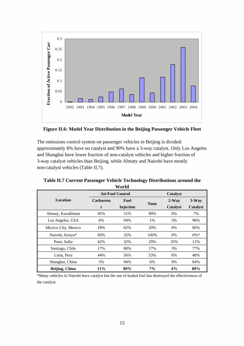
Figure II.6: Model Year Distribution in the Beijing Passenger Vehicle Fleet
The emissions control system on passenger vehicles in Beijing is divided: approximately 8% have no catalyst and 90% have a 3-way catalyst. Only Los Angeles and Shanghai have lower fraction of non-catalyst vehicles and higher fraction of 3-way catalyst vehicles than Beijing, while Almaty and Nairobi have mostly non-catalyst vehicles (Table II.7).
Table II.7 Current Passenger Vehicle Technology Distributions around the World
Air/Fuel Control Catalyst Location Carbureto
r Fuel
Injection None
2-Way Catalyst
3-Way Catalyst
Almaty, Kazakhstan 45% 51% 89% 0% 7% Los Angeles, USA 6% 94% 1% 3% 96%
Mexico City, Mexico 18% 82% 20% 0% 80%
Nairobi, Kenya* 60% 32% 100% 0% 0%* Pune, India 42% 32% 29% 35% 11%
Santiago, Chile 17% 80% 17% 3% 77% Lima, Peru 44% 56% 53% 6% 40%
Shanghai, China 5% 94% 6% 9% 84%
Beijing, China 11% 89% 7% 4% 89%
*Many vehicles in Nairobi have catalyst but the use of leaded fuel has destroyed the effectiveness of the catalyst.
15

II.C.3. Passenger Vehicle Use Odometer data was obtained from the parking lot surveys. Thus, some approximation of the use of individual vehicles can be made and this can be extrapolated to make approximations of total vehicle use for Beijing. Since there are few data of more than 8 years old vehicle, data from vehicles older than 8 years was not used in the analysis. Figure II.7 shows the passenger vehicle use taken from vehicle odometers.
y = -268.46x2 + 19144x
R2 = 0.986
0
20000
40000
60000
80000
100000
120000
140000
160000
0 2 4 6 8
Vehicle Age [yrs]
Odo
met
er [k
m]
10
Figure II.7: Passenger Vehicle Use during the first eight years of age
As is typical for the United States and all other countries studied so far, vehicle use decreases with vehicle age. Using the age distribution illustrated in previous Figure II.6, the average passenger car age in Beijing is approximately 4 years. Considering this figure and from the data analysis in Beijing, it is estimated that the overall average driving for Beijing passenger cars is 16,974 km/year. This translates to an average daily driving of 46.5 kilometers over the year (assuming 365 days/year). Based on the preceding vehicle driving estimates, the current travel in Beijing is approximated to be 109,568,844 kilometers per day in the Beijing Metropolitan Area1. This estimate is used in the IVE analysis to project emissions for the whole city. Table II.8 below provides the estimated total driving based on measurements made in this study.
1 This calculation is based on a total passenger car fleet of 1,704,531 vehicles driving 47 km/day, and 63,000 taxies driving 361 km/day, plus 22,696 buses driving 187 km/day, and 36,900 trucks driving 90km/day. Fleet estimates are based on data provided by www.bjbus.com; www.auto.hc360.com/dq/dq/tjsj5.htm; www.china.org.cn/chinese/2004/jul/608178.htm.
16

Table II.8: Observed Travel Distribution by vehicle type in Beijing
Type of Vehicle Fraction of
Observed Travel, 2004
Estimated Travel (km/day)
Thousands
Estimated Total Driving for all Categories in Beijing (N*A/f)(kms/day)
Passenger Car 70% 79,261 113229559 Taxi 24% 22,743 94762500 Bus 4% 4,244 106103800
Truck 2% 3,321 166050000 Total 100.00% 109,569
The values shown in Table II.8 should only be treated as approximate, but they should be in the ballpark of the true total driving occurring in Beijing in 2004. A final issue of interest is to compare Beijing driving with other areas. Figure II.8 illustrates the total driving per vehicle for the countries studied to date. As can be seen, passenger cars are driven the most in the United States, and the least in Sao Paulo, Brazil. Beijing has the second highest travel per passenger car. For the first 8 years of age, Beijing has a similar mileage pattern for passenger vehicles to the driving observed in Nairobi, Kenya. The data becomes unreliable after 10-12 years due to the uncertainty on the odometer readings and few data points.
0
50,000
100,000
150,000
200,000
250,000
300,000
0 2 4 6 8 10 12 14
Vehicle Age (yrs)
Accu
mul
ated
Odo
met
er R
eadi
ng (K
ms)
Los AngelesNairobiBeijingAlmatyLimaSantiagoMexico CityPuneSao PauloShanghai
Figure II.8: Comparison of Passenger Vehicle Use in different cities
Figure II.9 illustrates the average age of the on-road vehicle fleet in different cities where the IVE methodology has been carried out.
17

3.6 44.7
6.4 6.5 6.6
10.98 11.3
13.2
0
2
4
6
8
10
12
14
Shanghai
,China
Beijing,C
hina
Pune,
India
Mexico
City,M
exico
Santi
ago,Chil
e
Los Angel
es,USA
Lima,P
eru
Almaty
,Kaza
khstan
Nafrobi,
Kenya
Ave
rage
Age
(yrs
)
Figure II.9: Comparison of Average Vehicle Age in different cities
II.C.4. Taxi Vehicle Technology Distribution From Table II.3 we can see that taxi vehicles accounted for 24% of all the travel on urban roadways in Beijing, which is second only to Shanghai. In the end, almost 60 taxi vehicles were surveyed in detail to determine the fuel and technology characteristics. Table II.9 indicates some of the general characteristics observed in the surveyed fleet.
Table II.9: General characteristics of the surveyed Taxi Vehicles Type of Fuel* Type of Transmission Catalytic Converter (CC) 71.9% Gasoline 79% Mechanic Trans. 12.3% without CC 15.8%CNG/LPG 21% Automatic Trans. 87.7% with CC 7% Propane 5.3%Natural Gas
The distribution of the main technology types for gasoline taxi vehicles is shown in Table II.10.
Table II.10: IVE technology fractions of the Gasoline Taxi Vehicles
Taxi Fraction of
Passenger Taxi
Gasoline, Carburetor, No Catalyst 9.8% Gasoline, Carburetor, 2-way Catalyst 7.2%
Gasoline, Single Point Fuel Injection, 3-way Catalyst 9.8% Gasoline, Multipoint Fuel Injection, 3-way Catalyst 73.2%
18

The engine size of the Beijing taxi fleet was generally of a small size (<1501cc). And the taxies are heavily used in Beijing. Taxis drive an average of 361 kilometer through 18 hours per day. Table II.11 indicates the engine size and use distribution of the taxi.
Table II.11: Size and Use Characteristics of the Surveyed Passenger Car Fleet
Taxi Engine Size 8.8% Low Use
(<80 K km) 17.5% Medium Use
(80-161 K km) 73.7% High Use
(>161 K km) 78.9% Small (<1501 cc) 7% 10.5% 61.4%
21.1% Medium (1501-3000 cc) 1.8% 7% 12.3%
From the Table II.11 we can see that taxies are used frequently and most of them are small sized engines. The survey indicated no large sized taxis. Actually, there are larger taxis operating in Beijing, but they represent a low fraction in the fleet so they did not turn up in our surveys. At the same time, information in Table II.11 must be combined with information in Tables II.10 and the video collected data in Table II.2 to produce the taxi information for estimating emissions. Figure II.10 illustrates the model year distribution for taxi in Beijing. The average age of taxies in detailed survey was 4.92 years. And this data should be improved by collecting additional data concerning taxis since they are an important part of the Beijing fleet.
0
0.05
0.1
0.15
0.2
0.25
0.3
1997 1998 1999 2000 2001 2002 2003 2004
M o d e l Y e a r
Fraction of active taxie
Figure II.10: Model Year Distribution in the Beijing Taxi Fleet
19

II.C.5. Bus Vehicle Technology Distribution Although the number of private passenger cars has amounted to 1704 thousand and subways are capable of transporting great number of people, still a large number of people take buses as their main transportation tools. Up to now there are 22696 buses owned by mainly four large bus companies operating in Beijing. A total number of 601 buses were surveyed in large bus stations which were very close to railway stations, subway stations as well as fuel stations in different areas of Beijing. The buses there are supposed to send out all kinds of buses to various parts of Beijing which could well represent the overall bus technology distribution of Beijing. Table II.12 indicates the general characteristics observed in the survey.
Table II.12 General Characteristics of the surveyed Bus Vehicles Type of Fuel Air Conditioning System Exhaust Control 54.08% Petrol 30.28% with A/C 16.81% None 19.47% Diesel 69.72% without A/C 61.23% 3-way
6.82%LPG 3.33% Euro I
19.63% Natural Gas 15.14 % Euro II
3.49% Euro Ⅲ
Table II.13 indicates the detailed IVE technology fractions in the surveyed fleet.
Table II.13: IVE Technology Fractions of the Buses Fuel Air/Fuel Control Exhaust Control Fraction
Carburetor None 8.15% Carburetor 3-way 11.65%
Fuel Injection 3-way 25.96% Fuel Injection Euro I 3.33%
Petrol
Fuel Injection Euro II 4.99% Carburetor None 2.66%
CNG Fuel Injection 3-way 16.81%
Direct Injection None 5.99% Fuel Injection Euro II 10.15% Diesel Fuel Injection Euro Ⅲ 3.49%
LPG Fuel Injection 3-way 6.82%
More and more new buses with advanced exhaust control equipments and high requirements on clean fuels (CNG, LPG) are presented on the roads of Beijing. Meanwhile the government and bus companies are striving to abandon those old buses which account for 8.9% of the total number and have been driven for more than 10 years.
20

Buses in Beijing traveled about 180 km per day. Most of the buses were generally midsize (14,001 to 33,000 lbs GVWR) on the size. Table II.14 indicates the bus size and use distribution of the bus fleet.
Table II.14: Size and Use Characteristics of the Surveyed Bus Fleet
Vehicle Engine Size 35.8%Low
Use (<80 K km)
22.1%Medium Use
(80-160 K km)
42.1%High Use
(>160 K km) 76.2% Medium (14,001 to 33,000 lbs
GVWR) 18.8% 18.6% 38.8%
23.8% Large (>33,001 lbs GVWR) 17% 3.5% 3.3%
II.C.6. Truck Vehicle Technology Distribution The video tapes provided good estimates of the fractions of trucks on the road. However, the video tapes were not useful in establishing the engine technologies for trucks. It is difficult to get the detailed technology distribution in trucks of interest compared with passenger cars and taxies which could be easily available in parking lots. Truck technology distribution data was collected by interviewing several large truck companies. There were 101 trucks involved in the study. Table II.15 indicates the IVE technology fractions for Beijing trucks.
Table II.15: IVE Technology Fractions of the Trucks Fuel Air/Fuel Control Exhaust Control Fraction
Petrol Carburetor None 25.7% Direct Injection Improved 50.5% Fuel Injection Euro I 9.9% Diesel Fuel Injection EuroⅡ 13.9%
From Table II.15, we can see that 74.3% of tucks in Beijing use diesel as fuel. And trucks with high emission standard have account for a small part of the whole fleet. Table II.16 indicates the weight size and use distribution of the truck fleet. Half of the trucks are of medium size (9,000 to 14,000 lbs GVWR) and only 9.9% is of large size (14,001 to 33,000 lbs GVWR) which is comparatively new and equipped with satisfactory exhaust control measures. Generally, trucks in Beijing have been used for many years and mainly traveled in suburban areas outside the center of Beijing during daytime. Trucks in Beijing travel different distances per day, but the average daily travel is about 90 km per day.
21

Table II.16: Size and Use Characteristics of the Surveyed Truck Fleet
Vehicle Wight 27.7% Low
Use (<80 K km)
18.8% Medium Use
(80-160 K km)
53.5% High Use
(>160 K km) 37.6% Light (9,000 to 14,000 lbs
GVWR) 6.9% 6.9% 23.8% 52.5% Medium (14,001 to 33,000 lbs
GVWR) 13.9% 8.9% 29.7% 9.9% Large (>33,001 lbs GVWR) 6.9% 3% 0.00%
There is an increasing tendency that from 2002 trucks which meet Euro Ⅱ are more frequently used, meanwhile the older trucks with carburetors and no exhaust control measures are gradually abandoned. This trend will help to improve truck emissions in Beijing.
22

III. VEHICLE DRIVING PATTERNS III.A. BACKGROUND AND OBJECTIVES The main objective of this section is to collect second-by-second information on the speed and acceleration of the main types of vehicles operating in Beijing on a representative set of roadways throughout the day. III.B. METHODOLOGY Vehicle driving patterns were measured using GPS technology as described in Appendix A. This technology allows the measurement of each second of vehicle location, speed, and altitude. Three representative sections of the city were selected for the IVE study in Beijing. The areas selected represented a generally lower income area, a generally upper income area, and a commercial area of the city. The passenger cars were driven along selected roads, while the trucks, taxes and buses were operated on their normal daily route throughout Beijing. Figure II.1 and Table III.1 show the sectors and streets selected in this study for measurement of passenger vehicles.
Table III.1 Streets selected for passenger vehicle driving in Beijing, China Street Type Location
Highway A1 Huixin Dong Road
Highway B1 Fu Chengmen Road
Highway C1 Yang Bridge
Arterial A2 Huixin Dong St.
Arterial B2 Xi Dan Culture Squre
Arterial C2 Ma Jiaobao Dong Rd.
Residential A3 Xiaoying Bei Rd.
Residential B3 Yue Tan Bei St.
Residential C3 Ma Jiabao St.
Figure III.1 illustrates the driving locations collected from one of the CGPS installed on a passenger car driving over the three sectors in Beijing. The different street types are indicated by different colors.
23
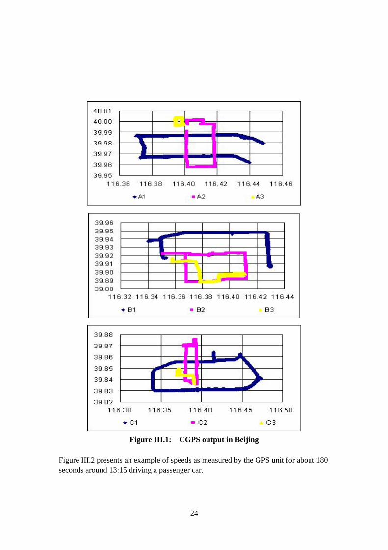
Figure III.1: CGPS output in Beijing
Figure III.2 presents an example of speeds as measured by the GPS unit for about 180 seconds around 13:15 driving a passenger car.
24

0
10
20
30
40
50
60
70
13:13:03 13:13:46 13:14:29 13:15:13 13:15:56Time [hh:mm:ss]
Velocity [kph]
Highway Arterial Residential
Figure III.2: Example of Residential, Arterial, and Highway Driving at 13:15 in Beijing
Figure III.3 presents an example of altitude and velocity recorded from a passenger car over a 30 minutes drive. The altitude reading is the least certain of the data collected by a GPS unit, but it is still useful for estimating road grade. Basically, the grade change of road in Beijing is not very sharp, it always change when vehicles pass through an over bridge.
0102030405060708090
12:05:00 12:12:12 12:19:24 12:26:36 12:33:48
Time [hh:mm:ss]
Alti
tude
[m]
0510152025303540
Spee
d [k
mph
]
Altitude speed
Figure III.3: Example of Altitude and Speed Recorded by GPS over a 30
Minutes Drive In using this data to estimate road grade, care must be taken to look at multiple adjacent sample points to make the most appropriate estimate of road grade. The IVE model uses a calculation of the power demand on the engine per unit vehicle mass to correct for the driving pattern impact on vehicle emissions. This power factor is called vehicle specific power (VSP). The VSP is the best, although imperfect,
25
indicator of vehicle emissions relative the vehicles base emission rate. Equation III.1 presents the VSP equation used. VSP = 0.132*S + 0.000302*S2 + 1.1*S*dS/dt + 9.81*Atan(Sin(Grade)) III.1 Where,
S = vehicle speed in km/second. dS/dt = vehicle acceleration km/second/second. Grade = grade of road grade radians.
About 65% of the variance in vehicle emissions can be accounted for using VSP. To further improve the emissions correction for vehicle driving, a factor denoted vehicle stress was developed. Vehicle stress (STR) uses an estimate of vehicle RPM combined with the average of the power exerted by the vehicle in the 15 seconds before the event of interest. Equation III.2 indicates the calculation for STR.
STR=RPM + 0.08*PreaveragePower III.2 Where,
RPM = the estimated engine RPM/1000 (an algorithm was developed by driving many different vehicles and measuring RPM compared to vehicle speed and acceleration. The minimum RPM allowed is 900. PreaveragePower = the average of VSP the 15 seconds before the time of interest. The 0.08 coefficient was developed from a statistical analysis of emissions and speed data from about 500 vehicles to give the best correction factor when combined with VSP.
Ultimately, the GPS data for each vehicle type studied is broken into one of 20 VSP bins and one of 3 STR Bins. Thus, each point along the driving route can be allocated to one of 60 driving bins. A given driving trace can be evaluated to indicate the fraction of driving that occurs in each driving bin. These fractions are used to develop a correction factor for a given driving situation. III.C. RESULTS III.C.1. Passenger Cars Data on passenger car driving was collected in three parts of Beijing (see Table II.1) over six days. Table III.2 indicates the average speed for each type of road studied for each 2-hour group.
26

Table III.2: Average Passenger Car Speeds on Beijing Roads Time Highway Arterial Residential Street 05:30 38.75 19.46 16.36 07:30 33.54 19.46 16.36 09:30 36.11 15.89 17.98 11:30 28.38 16.41 13.47 13:30 38.65 21.75 15.71 15:30 35.68 14.42 16.40 17:30 40.61 16.40 13.03 19:30 31.90 19.69 14.57
Speed is not a good indicator of vehicle power demand. Vehicle acceleration consumes considerable energy and is not indicated by average vehicle speed. Tables III.3 to III.5 below provide the power bin distribution for the driving on Beijing Highways, Arterials, and Residential streets respectively averaged over all hours. For use in the IVE model, the power bin distributions can also be used in the two hour groupings indicated in Table III.3 to make hourly estimates of emissions from passenger vehicles. It should be noted that Power Bins 1-11 represent the case of negative power (i.e. the vehicle is slowing down or going down a hill or some combination of each). Power Bin 12 represents the zero or very low power situation such as waiting at a signal light. Power Bins 13 and above represent the situation where the vehicle is using positive power (i.e. driving at a constant speed, accelerating, going up a hill or some combination of all three).
Table III.3: Distribution of driving into IVE Power Bins for passenger cars operating on Highways averaged over all hours
(average speed: 36.15 km/hour) Stress
Group Power Bins
1 2 3 4 5 6 7 8 9 10
0.05% 0.01% 0.00% 0.02% 0.02% 0.04% 0.07% 0.16% 0.41% 1.17%
11 12 13 14 15 16 17 18 19 20 Low
6.00% 40.73% 34.15% 12.33% 3.17% 0.77% 0.07% 0.05% 0.02% 0.06%
1 2 3 4 5 6 7 8 9 10
0.00% 0.00% 0.00% 0.00% 0.00% 0.00% 0.00% 0.00% 0.00% 0.00%
11 12 13 14 15 16 17 18 19 20 Med
0.00% 0.01% 0.01% 0.01% 0.00% 0.25% 0.24% 0.05% 0.02% 0.07%
1 2 3 4 5 6 7 8 9 10
0.00% 0.00% 0.00% 0.00% 0.00% 0.00% 0.00% 0.00% 0.00% 0.00%
11 12 13 14 15 16 17 18 19 20 High
0.00% 0.00% 0.00% 0.00% 0.00% 0.00% 0.00% 0.00% 0.00% 0.00%
27

Table III.4: Distribution of Driving into IVE Power Bins for Passenger Cars Operating on Arterials Averaged Over All Hours
(average speed: 16.16 km/hour) Stress
Group Power Bins
1 2 3 4 5 6 7 8 9 10
0.02% 0.02% 0.02% 0.02% 0.03% 0.07% 0.09% 0.26% 0.53% 1.64%
11 12 13 14 15 16 17 18 19 20 Low
6.62% 61.49% 19.47% 6.74% 1.97% 0.56% 0.16% 0.06% 0.04% 0.06%
1 2 3 4 5 6 7 8 9 10
0.00% 0.00% 0.00% 0.00% 0.00% 0.00% 0.00% 0.00% 0.00% 0.00%
11 12 13 14 15 16 17 18 19 20 Med
0.00% 0.00% 0.00% 0.00% 0.00% 0.05% 0.06% 0.02% 0.00% 0.02%
1 2 3 4 5 6 7 8 9 10
0.00% 0.00% 0.00% 0.00% 0.00% 0.00% 0.00% 0.00% 0.00% 0.00%
11 12 13 14 15 16 17 18 19 20 High
0.00% 0.00% 0.00% 0.00% 0.00% 0.00% 0.00% 0.00% 0.00% 0.00%
Table III.5: Distribution of Driving into IVE Power Bins for Passenger Cars
Operating on Residential Streets Averaged Over All Hours (average speed: 15.5 km/hour)
Stress
Group Power Bins
1 2 3 4 5 6 7 8 9 10
0.02% 0.00% 0.01% 0.01% 0.02% 0.03% 0.06% 0.11% 0.35% 1.30%
11 12 13 14 15 16 17 18 19 20 Low
6.13% 60.26% 23.97% 5.80% 1.34% 0.30% 0.11% 0.06% 0.02% 0.06%
1 2 3 4 5 6 7 8 9 10
0.00% 0.00% 0.00% 0.00% 0.00% 0.00% 0.00% 0.00% 0.00% 0.00%
11 12 13 14 15 16 17 18 19 20 Med
0.00% 0.00% 0.00% 0.00% 0.00% 0.00% 0.02% 0.00% 0.00% 0.02%
1 2 3 4 5 6 7 8 9 10
0.00% 0.00% 0.00% 0.00% 0.00% 0.00% 0.00% 0.00% 0.00% 0.00%
11 12 13 14 15 16 17 18 19 20 High
0.00% 0.00% 0.00% 0.00% 0.00% 0.00% 0.00% 0.00% 0.00% 0.00%
It is clear looking at Tables III.3 through III.5 that the times in the zero power bin12, (stopping and idling) increases from the highway to arterial driving. It is also noteworthy that no high stress driving was observed for passenger vehicles in Beijing; although, some medium stress and high power bin driving was observed.
28

III.C.2. Taxis Several taxis were equipped with the GPS units and allowed to drive their normal daily routes. The vehicles were not restricted to specific streets. They were simply asked to operate their vehicles as they normally would pick up passengers and dropping them off over the Beijing Metropolitan area. Table III.6 shows the average speeds recorded for the taxis.
Table III.6: Average Taxi Speeds on Beijing Roads Time Overall
5:30 32.49 7:30 32.49 9:30 16.99
11:30 21.71 13:30 13.69 15:30 24.15 17:30 29.20 19:30 29.20
The taxi speeds are, as expected, similar to a combination of highway and arterial driving from passenger vehicles. Similar congestion patterns are observed in the taxi driving patterns as the passenger vehicles in terms of steadily increasing congestion and lowering average velocities throughout the day, with the minimum speed occurring between 12:30 and 14:30. Table III.7 presents the power-binned data for the taxis averaged over all hours.
Table III.7: Distribution of Driving into IVE Power Bins for Taxis Averaged Over All Hours (average speed: 19.76 km/hour)
Stress
Group Power Bins
1 2 3 4 5 6 7 8 9 10
0.01% 0.00% 0.00% 0.01% 0.02% 0.04% 0.09% 0.24% 0.61% 1.59%
11 12 13 14 15 16 17 18 19 20 Low
5.25% 60.34% 19.23% 8.94% 2.83% 0.50% 0.06% 0.02% 0.01% 0.02%
1 2 3 4 5 6 7 8 9 10
0.00% 0.00% 0.00% 0.00% 0.00% 0.00% 0.00% 0.00% 0.00% 0.00%
11 12 13 14 15 16 17 18 19 20 Med
0.00% 0.00% 0.00% 0.00% 0.01% 0.06% 0.06% 0.02% 0.01% 0.01%
1 2 3 4 5 6 7 8 9 10
0.00% 0.00% 0.00% 0.00% 0.00% 0.00% 0.00% 0.00% 0.00% 0.00%
11 12 13 14 15 16 17 18 19 20 High
0.00% 0.00% 0.00% 0.00% 0.00% 0.00% 0.00% 0.00% 0.00% 0.00%
29
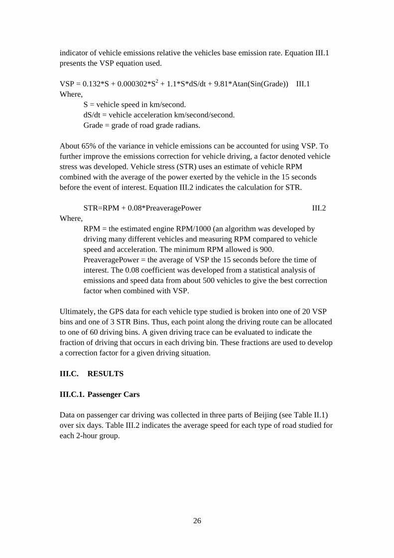
III.C.3. Buses Table III.8 indicates average Bus vehicle speeds in Beijing. The bus speeds are relatively constant throughout the day compared with passenger vehicles and taxis.
Table III.8: Average Bus Speeds on Beijing Roads Time Overall
05:30 14.63 07:30 16.84 09:30 16.36 11:30 19.53 13:30 17.75 15:30 15.72 17:30 15.38 19:30 18.45
Table III.9 indicates the power bin distributions for a bus averaged over all hours. Table III.9: Distribution of Driving into IVE Power Bins Buses Averaged Over
All Hours (average speed: 17.07 km/hour) Stress
Group Power Bins
1 2 3 4 5 6 7 8 9 10
0.01% 0.00% 0.01% 0.01% 0.01% 0.03% 0.05% 0.15% 0.40% 1.47%
11 12 13 14 15 16 17 18 19 20 Low
5.58% 58.34% 26.87% 5.96% 0.72% 0.17% 0.06% 0.03% 0.03% 0.04%
1 2 3 4 5 6 7 8 9 10
0.00% 0.00% 0.00% 0.00% 0.00% 0.00% 0.00% 0.00% 0.00% 0.00%
11 12 13 14 15 16 17 18 19 20 Med
0.00% 0.01% 0.00% 0.00% 0.00% 0.01% 0.01% 0.00% 0.00% 0.02%
1 2 3 4 5 6 7 8 9 10
0.00% 0.00% 0.00% 0.00% 0.00% 0.00% 0.00% 0.00% 0.00% 0.00%
11 12 13 14 15 16 17 18 19 20 High
0.00% 0.00% 0.00% 0.00% 0.00% 0.00% 0.00% 0.00% 0.00% 0.00%
30

III.C.4. Trucks Table III.10 indicates average truck vehicle speeds in Beijing. The maximum speed is during in the early morning and evening. It is noteworthy that trucks are not allowed to pass inside the 4th Ring Road in Beijing during daytime from 7 am to 9 pm. So the trucks that we equipped with GPS traveled to wherever the driver needed to drive thus the date listed below during daytime could not reflect the travel situation inside the 4th Ring Road.
Table III.10: Average Delivery Truck Speeds on Beijing Roads Time Overall
05:30 24.59
07:30 24.59
09:30 10.03
11:30 21.71
13:30 13.69
15:30 24.15
17:30 7.58
19:30 24.59
Table III.11 indicates the power bin distributions for the trucks averaged over all hours. A large fraction of the truck driving pattern is spent idling. The times in the zero power bin12 is similar with the time of passenger vehicles in arterial way.
Table III.11: Distribution of Driving into IVE Power Bins Trucks Averaged Over All Hours (average speed: 17.18km/hour)
Stress
Group Power Bins
1 2 3 4 5 6 7 8 9 10
0.00% 0.00% 0.00% 0.00% 0.01% 0.02% 0.05% 0.15% 0.37% 1.02%
11 12 13 14 15 16 17 18 19 20 Low
3.42% 68.14% 17.40% 7.26% 1.92% 0.17% 0.01% 0.01% 0.00% 0.00%
1 2 3 4 5 6 7 8 9 10
0.00% 0.00% 0.00% 0.00% 0.00% 0.00% 0.00% 0.00% 0.00% 0.00%
11 12 13 14 15 16 17 18 19 20 Med
0.00% 0.00% 0.00% 0.00% 0.00% 0.01% 0.02% 0.01% 0.00% 0.01%
1 2 3 4 5 6 7 8 9 10
0.00% 0.00% 0.00% 0.00% 0.00% 0.00% 0.00% 0.00% 0.00% 0.00%
11 12 13 14 15 16 17 18 19 20 High
0.00% 0.00% 0.00% 0.00% 0.00% 0.00% 0.00% 0.00% 0.00% 0.00%
31

III.C.5. Summary of Driving Pattern Results Figure III.4 compares driving speeds by hour for the four types of vehicles studied. In general, congestion lowers the average velocity during the daytime hours by 30 to 60 percent of free flow velocities. It was assumed that the early morning and late evening velocities were similar to the late evening and 6 AM data because no data was collected between 10 pm and 5 am. Overall, passenger vehicles have the fastest velocities on the highways. The lowest velocity occurs in trucks. Buses, trucks and taxis have similar average speeds to passenger vehicles traveling on arterial roadways. Trucks have very high velocities during the middle of the day, because most of the trucks are driven in the suburban during the daytime. Taxis and passenger vehicles operating on the highway during the middle of the day and evening exhibit the highest occurrences of hard accelerations, due to congestion and high target velocities.
0
5
10
15
20
25
30
35
40
45
50
0:00
1:00
2:00
3:00
4:00
5:00
6:00
7:00
8:00
9:00
10:00
11:00
12:00
13:00
14:00
15:00
16:00
17:00
18:00
19:00
20:00
21:00
22:00
23:00
Time of Day (hh:mm)
Aver
age
Vel
ocity
(kph
)
PCHwy PCRes PCArt 2wArt Taxi Bus DTruck
Figure III.4: Average Speeds for All Road Types and Vehicle Classes in Beijing Figure III.5 shows the distribution into driving bins for four of the main classes of driving at 07:30. There is little to distinguish the driving patterns between passenger vehicles and buses at this time of the morning. The trucks have the highest percentage of idling.
32

0%
10%
20%
30%
40%
50%
60%
70%
80%
90%
1 3 5 7 9 11 13 15 17 19 21 23 25 27 29 31 33 35 37 39 41 43 45 47 49 51 53 55 57 59
VSP/Stress Bin
Per
cent
of
Driv
ing.
PCHwy PCRes PCArt Taxi 2wArt DTruck Bus
Figure III.5: Comparison of Driving Patterns for Five Major Vehicle Classes for 07:30
Figure III.6 represents driving at 12:30. In this case, the highway passenger vehicles and taxi driving contain some higher power driving (bins above 20) which is caused by hard accelerations. The highway driving contains the lowest percentage of idle and low stress driving, while the arterial way driving contains the highest percentage of idle. Arterial way driving is significantly different and contain more idle time than the early morning.
33

0%
10%
20%
30%
40%
50%
60%
70%
1 3 5 7 9 11 13 15 17 19 21 23 25 27 29 31 33 35 37 39 41 43 45 47 49 51 53 55 57 59VSP/Stress Bin
Per
cent
of
Driv
ing.
PCHwy PCRes PCArt Taxi 2wArt DTruck Bus
Figure III.6: Comparison of Driving Patterns for Five Major Vehicle Classes
for 12:30 Figure III.7 represents the 17:30 time frame. This hour of the day represents the most different driving among the various vehicle classes. Highway driving has some high stress driving.
34

0%
10%
20%
30%
40%
50%
60%
70%
80%
90%
1 3 5 7 9 11 13 15 17 19 21 23 25 27 29 31 33 35 37 39 41 43 45 47 49 51 53 55 57 59
VSP/Stress Bin
Per
cent
of
Driv
ing.
PCHwy PCRes PCArt Taxi 2wArt DTruck Bus
Figure III.7: Comparison of Driving Patterns for Five Major Vehicle Classes for 17:30
Data sets using the binned data and average speeds are used in the IVE model to correct emission estimates for local driving patterns.
35

IV. VEHICLE START PATTERNS IV.A. BACKROUND AND OBJECTIVES Between10% and 30% of vehicle emissions come from vehicle starts in the United States and likely elsewhere. This is a significant amount of emissions. Thus, it is important to understand vehicle start patterns in an urban area to fully evaluate vehicle emissions. To measure start patterns, a small device that plugs into the cigarette lighter or otherwise hooks into a vehicles electrical system has been developed (VOCE units). The voltage fluctuations in the electrical system can be used to estimate when a vehicle engine is on and off. This process is described in Appendix A. The main objective of this section is to collect a representative sample of the number, time of day, and soak period from passenger vehicle start-ups in Beijing. IV.B. METHODOLOGY The vehicle engine start patterns were collected using equipment that senses vehicle system voltage denoted VOCE units. VOCE data can be used to determine when vehicles start, how long they operate, and how long they sit idle between starts. This information is essential to establish vehicle start emissions. The VOCE units were placed in passenger vehicles and left there for 9 days. IV.C. RESULTS Table IV.1 indicates the measured start and soak patterns for passenger vehicles in Beijing. Data was successfully collected from about 75 passenger vehicles over about 9 days for each vehicle. This provides about 630 vehicle days of data. Problems were found with the data from 25 VOCE units. Thus, data from 50 VOCE units was processed to measure start and soak time distributions. While this amount of information is significant, it is possible that hour by hour data would include too few events and would be meaningless, so the data was lumped into 2 hour groups.
36
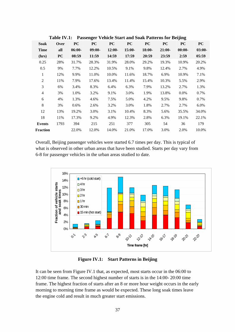
Table IV.1: Passenger Vehicle Start and Soak Patterns for Beijing
Soak Time (hrs)
Overall PC
PC 06:00- 08:59
PC 09:00- 11:59
PC 12:00- 14:59
PC 15:00- 17:59
PC 18:00- 20:59
PC 21:00- 23:59
PC 00:00- 2:59
PC 03:00- 05:59
0.25 28% 31.7% 28.3% 31.9% 28.0% 29.2% 19.3% 10.9% 20.2% 0.5 9% 7.7% 12.2% 10.5% 9.1% 9.8% 12.4% 2.7% 4.9% 1 12% 9.9% 11.0% 10.0% 11.6% 18.7% 6.9% 10.9% 7.1% 2 11% 7.9% 17.6% 13.4% 11.4% 15.4% 10.3% 5.5% 2.9% 3 6% 3.4% 8.3% 6.4% 6.3% 7.9% 13.2% 2.7% 1.3% 4 3% 1.0% 3.2% 9.1% 3.0% 1.9% 13.8% 0.0% 0.7% 6 4% 1.3% 4.6% 7.5% 5.0% 4.2% 9.5% 9.8% 0.7% 8 3% 0.6% 2.6% 3.2% 3.0% 1.8% 2.7% 2.7% 6.0%
12 13% 19.2% 3.0% 3.1% 10.4% 8.3% 5.6% 35.5% 34.0% 18 11% 17.3% 9.2% 4.9% 12.3% 2.8% 6.3% 19.1% 22.1%
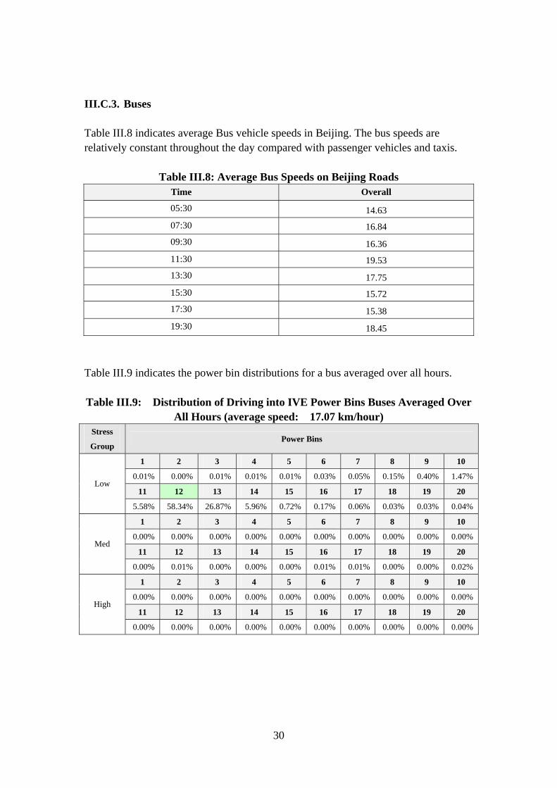
Events 1793 394 215 251 377 305 54 36 179 Fraction 22.0% 12.0% 14.0% 21.0% 17.0% 3.0% 2.0% 10.0% Overall, Beijing passenger vehicles were started 6.7 times per day. This is typical of what is observed in other urban areas that have been studied. Starts per day vary from 6-8 for passenger vehicles in the urban areas studied to date.
0%
2%
4%
6%
8%
10%
12%
14%
16%
0-1 2-3 4-5 6-7 8-910
-1112
-1314
-1516
-1718
-1920
-2122
-23
Time frame [hr]
Frac
tion
of v
ehic
le s
tart
san
d so
ak ti
mes
+6 hr (cold start)4 hr3 hr2 hr1 hr30 min15 min (hot start)
Figure IV.1: Start Patterns in Beijing
It can be seen from Figure IV.1 that, as expected, most starts occur in the 06:00 to 12:00 time frame. The second highest number of starts is in the 14:00- 20:00 time frame. The highest fraction of starts after an 8 or more hour weight occurs in the early morning to morning time frame as would be expected. These long soak times leave the engine cold and result in much greater start emissions.
37

V. IVE APPLICATION AND EMISSIONS RESULTS The fraction of driving per hour can be estimated using traffic counts shown in Table II.1 and averaged according to the fraction of driving on each type of street discussed in Section II.A. Based on the observed number of vehicles on the different road types and the total length of each type of road in Beijing, it was estimated that 23% of overall driving in Beijing is on arterials, 42% on highways, and 35% on residential streets. The results are shown in Table V.1. Since no data was collected between 0:00 and 06:00 and between 21:00 and 0:00 these values were estimated using fractions observed in other urban areas. In the case of vehicle starts, Tables IV.1 and IV.2 were weighted by the fraction of passenger vehicles. A total of approximately 2 million vehicles were assumed to be in daily operation in 2004 in the Beijing Metropolitan Area.
38

Table V.1: Estimated Fraction and VMT and Starts by Hour in the Beijing Metropolitan Area
Time of Day
Estimated Driving
Fractions in Each Hour
Total Estimated Driving by
Hour (kilometers)
Fraction of Starts in
Each Hour
Total Estimated Starts by
Hour 0:00 1% 1,424,969 1% 87,666 1:00 1% 870,210 1% 87,666 2:00 1% 587,392 1% 100,190 3:00 0% 445,983 1% 100,190 4:00 0% 413,350 1% 150,285 5:00 1% 598,269 1% 150,285 6:00 2% 1,664,276 6% 738,900 7:00 6% 6,182,699 6% 738,900 8:00 7% 7,634,254 7% 926,755 9:00 7% 7,251,096 7% 926,755
10:00 7% 7,812,040 6% 751,423 11:00 6% 6,644,378 6% 751,423 12:00 6% 6,372,016 5% 626,186 13:00 6% 6,428,104 5% 626,186 14:00 7% 7,328,727 6% 776,471 15:00 6% 6,786,383 6% 776,471 16:00 7% 7,273,536 6% 776,471 17:00 8% 8,644,560 6% 776,471 18:00 6% 6,559,202 6% 726,376 19:00 5% 5,788,479 6% 726,376 20:00 4% 4,712,279 3% 425,807 21:00 3% 3,263,287 3% 425,807 22:00 2% 2,175,525 2% 187,856 23:00 2% 2,175,525 2% 187,856
Total 109,036,536 12,548,769 The calculations shown above are for illustrative purposes only. They are approximations and more extensive measurements should be completed in Beijing to improve the estimate of total daily driving in Beijing and hourly driving outside of the hours measured in this study. Figure V.1 shows the modeling results using the data developed or estimated from this study for Carbon Monoxide. The top line reflects start and running emissions added together.
39

0
50
100
150
200
250
300
0 1 2 3 4 5 6 7 8 9 10 11 12 13 14 15 16 17 18 19 20 21 22 23
Hour of Day
Em
issi
ons
(tons
/hou
r)
RunningStart
Figure V.1: Overall Beijing Carbon Monoxide Emissions
The peak CO emissions are occurring around 17:30 and 19:00, because time from 17:00 to 19:00 is the rush hour for people going home. But an interesting thing is that there is no obvious peak in the early morning. That is caused by that the time people start work is not same in Beijing. Obviously, emissions are very low from 22:00 to 05:00. It is also valuable to note the importance of start emissions in Beijing. Most of the time, they represent approximately a quarter of vehicle CO emissions. Overall, Figure V.1 reflects a total of 2402 metric tons of CO emitted per day into the air over Beijing or an overall daily average emission rate of 22 grams/kilometer traveled including starting and running emissions. Figure V.2 shows the modeling results using the data developed or estimated from this study for volatile organic compounds (VOC) including evaporative emissions. The top line reflects start, running, and evaporative emissions added together.
40

0.0
2.0
4.0
6.0
8.0
10.0
12.0
14.0
16.0
18.0
20.0
0 1 2 3 4 5 6 7 8 9 10 11 12 13 14 15 16 17 18 19 20 21 22 23
Hour of Day
Em
issi
ons
(tons
/hou
r)
Evaporative
Running
Start
Figure V.2: Overall Beijing Volatile Organic Emissions
The peak VOC emission occurs at about 17:30. Start emissions are not as great a percentage of emissions as are the case for CO, but they are still large. Evaporative emissions are somewhat important as well. Figure V.2 reflects a total of 192 metric tons per day of VOC emissions going into the air over Beijing or an overall daily average emission rate of 1.8 grams/kilometer including starting, running, and evaporative emissions. Figure V.3 shows the modeling results using the data developed or estimated from this study for Nitrogen Oxides (NOx). The top line reflects start and running emissions added together. Figure V.3 reflects a total of 199 metric tons per day of NOx going into the air over Beijing or an overall daily average emission rate of 1.8 grams/kilometer including starting and running emissions.
41
0.0
5.0
10.0
15.0
20.0
25.0
0 1 2 3 4 5 6 7 8 9 10 11 12 13 14 15 16 17 18 19 20 21 22 23
Hour of Day
Em
issi
ons
(tons
/hou
r)
RunningStart
Figure V.3: Overall Beijing Nitrogen Oxide Emissions
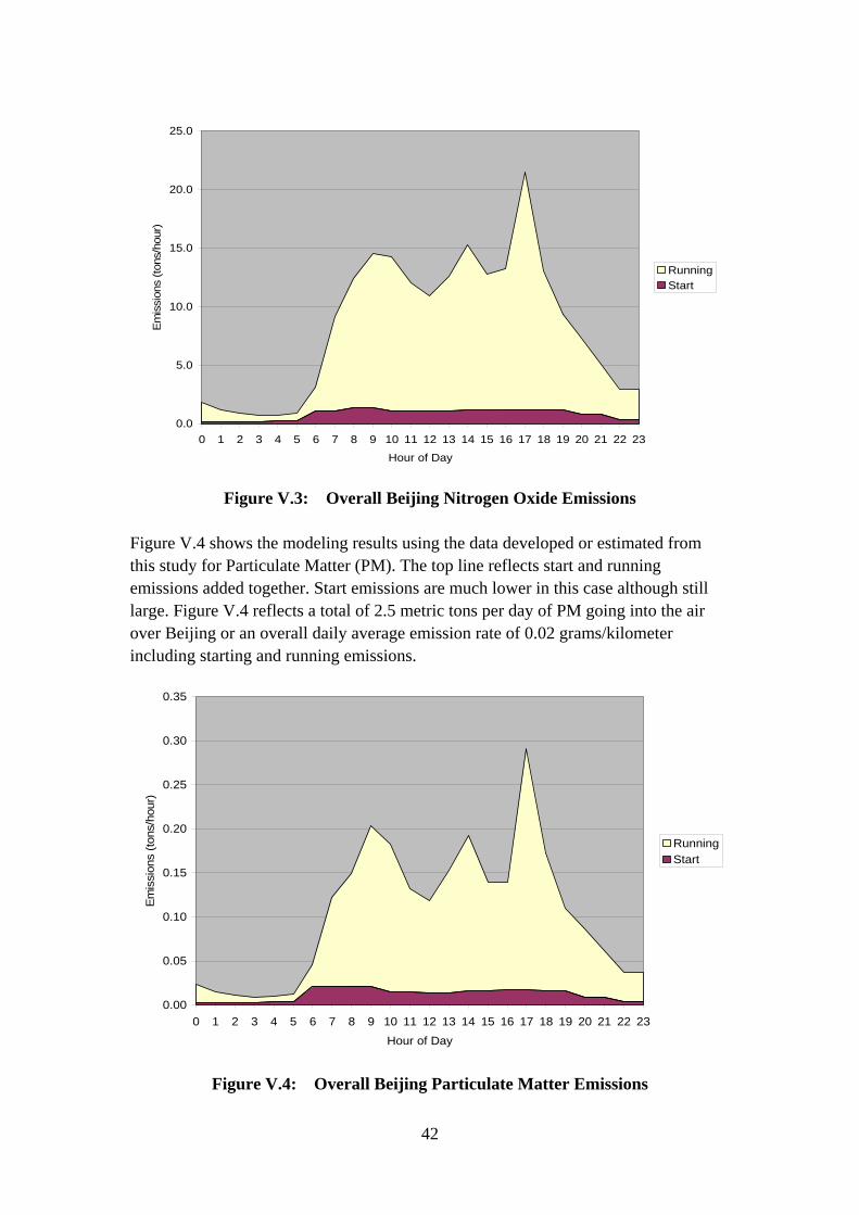
Figure V.4 shows the modeling results using the data developed or estimated from this study for Particulate Matter (PM). The top line reflects start and running emissions added together. Start emissions are much lower in this case although still large. Figure V.4 reflects a total of 2.5 metric tons per day of PM going into the air over Beijing or an overall daily average emission rate of 0.02 grams/kilometer including starting and running emissions.
0.00
0.05
0.10
0.15
0.20
0.25
0.30
0.35
0 1 2 3 4 5 6 7 8 9 10 11 12 13 14 15 16 17 18 19 20 21 22 23
Hour of Day
Emis
sion
s (to
ns/h
our)
RunningStart
Figure V.4: Overall Beijing Particulate Matter Emissions
42

VSP plays a very important role on vehicle emissions. Table V.2 indicates the emission rates of different vehicle pollutants from passenger cars on three road types. As can be seen, passenger cars on residential had the lowest velocity of 15.5 km/hr and passenger cars on arterials had the highest fraction of BIN 12, so the emission factors were much higher than on highways. Obviously driving activity has an important effect on the vehicle emissions, so enough concerns should be focused on traffic management in Beijing. Table V.2 Comparison of Emission Rate of Passenger Vehicles on Each Road
Types Emission Rate, g/km
Results Average Velocity
km/hr BIN12
% CO VOC Nox PM CO2 PCHighway 36.15 40.73 8.3 0.6 0.8 0.004 239.9
PCResidential 15.50 60.34 25.6 1.8 1.8 0.010 509.8 PCArterial 16.16 61.49 25.1 1.8 1.8 0.009 481.6
To better understand the emissions created from the Beijing vehicle fleet, it is useful to look at the contribution of each type of vehicle class. For Beijing, the major vehicle categories include light duty passenger vehicles (PC) and taxis (taxi), buses (Bus), and few trucks (Truck). The fraction of travel from each of these types of vehicles is shown in the last column of Figure V.5. The percent contribution each of these vehicle types to vehicular CO, VOC, NOx, PM, and CO2 emissions is also shown in Figure V.5. These results indicate that passenger cars are the main emission source in Beijing while buses and trucks also take up many travels in Beijing. The majority of vehicular CO, VOC, NOx, and CO2 are from passenger cars. Buses and trucks cause most of the PM emissions and also play an important role in NOx emission because of their relatively high emission rates.
43

0%
10%
20%
30%
40%
50%
60%
70%
80%
CO VOC NOX PM CO2 VMT
PC Taxi Buses Truck
Figure V.5 Emission Contribution of Each Vehicle Type in Beijing
Clearly, to reduce PM emissions in Beijing, buses and trucks must be controlled. To reduce other kinds of pollutants and CO2, passenger vehicles must be further addressed. Since year 2003, the number of passenger cars in Beijing has increased dramatically. And the high rate of increase will likely continue for a long period of time. Of course, the passenger vehicles produce a very large fraction of emissions. Thus it is important to determine the best approaches to controlling passenger cars, especially the private fleet as the key point to control vehicle emissions in Beijing. Another calculation that is of interest is the overall per kilometer emissions of Beijing vehicles compared to vehicle fleets in cities of other countries. Figure V.6 compares Beijing with data obtained from similar studies conducted in Los Angeles, Santiago, Mexico, Nairobi, Pune, and Shanghai. These locations have a very different profile of vehicle fleet, fuel type, and driving patterns.
44

0
2
4
6
8
10
12
14
CO/10 VOC NOx PM*10 CO2/40
Emis
sion
Fac
tors
(g/k
m)
Los Angeles Nairobi Santiago Pune Mexico Beijing Shanghai
Figure V.6: Comparison of Daily Average Emission Rates in Countries Studied
to Date The Beijing fleet has the third highest CO2 emissions and the lowest PM emissions. It is a moderate producer of CO, VOC and NOx. The lowest PM emissions are particularly because trucks are not allowed to drive on the streets inside of the 4th Ring Road between the hours of 7 am and 9 pm. Figure V.5 illustrates the possibilities that if passenger vehicles number was well controlled, significant emissions reductions for CO, VOC and NOx could be achieved in the Beijing area. If trucks were further controlled, PM and toxic emissions would be greatly reduced.
45

In conclusion, this study has developed basic data to allow for improved estimates of emissions from the Beijing fleet. Additional studies are needed to further improve emission estimates in China, but significant planning activities can occur using the data in this report. Our recommendations are as follows:
1. Update the total number of the passenger vehicles in operation in Beijing. Since 2003, the number of passenger cars in Beijing has increased dramatically. Additionally, improve the data on the total number of trucks and buses operating in the Beijing area.
2. Improve emission factors for in-use vehicles. Emission studies are needed to
verify the operating emissions of passenger vehicles, buses and trucks in Beijing to insure that the best emission factors are being used.
3. Select some routes near new construction areas and study night time activity
patterns to determine the truck’s activity fractions on the road fleet for more exact PM emission estimates.
4. Use advanced technology tools (ie. GIS mapping) to better determine the
fractions of each road type in Beijing.
5. Use the IVE model along with air quality measurements to map out a strategy for improved future air quality, and then seek to improve the air quality management process by further upgrading the Beijing database.
46


