Embed Size (px)
Citation preview

Name Designation Affiliation Date Signature
Additional Authors
Rob Ferdman, Ben Stappers
Submitted by:
A AhmedSaid UMAN 2011‐04‐01
Approved by:
W. Turner Signal Processing Domain Specialist
SPDO 2011‐03‐26
PULSAR SIGNAL PROCESSING ON UNIBOARD
Document number .................................................................. WP2‐040.170.010‐TD‐001
Revision ........................................................................................................................... 1
Author .......................................................................................................... A AhmedSaid
Date ................................................................................................................. 2011‐04‐01
Status ............................................................................................... Approved for release

WP2‐040.170.010‐TD‐001
Revision : 1
2011‐04‐01 Page 2 of 24
DOCUMENT HISTORY
Revision Date Of Issue Engineering Change
Number
Comments
A 1st April 2011 ‐ First draft release for internal review
1 1st April 2011
DOCUMENT SOFTWARE
Package Version Filename
Wordprocessor MsWord Word 2003 03m‐wp2‐040.170.010‐td‐001‐1‐pulsar SP on Uniboard‐2003
Block diagrams
Other
ORGANISATION DETAILS
Name SKA Program Development Office
Physical/Postal
Address
Jodrell Bank Centre for Astrophysics
Alan Turing Building
The University of Manchester
Oxford Road
Manchester, UK
M13 9PL
Fax. +44 (0)161 275 4049
Website www.skatelescope.org

WP2‐040.170.010‐TD‐001
Revision : 1
2011‐04‐01 Page 3 of 24
TABLE OF CONTENTS
1 INTRODUCTION ............................................................................................. 6
1.1 Purpose of the document ....................................................................................................... 6
2 REFERENCES ................................................................................................ 7
3 OVERVIEW .................................................................................................. 8
4 APPLICATIONS OF UNIBOARD TO RADIO PULSAR OBSERVING ................................. 8
5 DESIGN METHODOLOGY ................................................................................. 9
5.1 Algorithmic Simulation ............................................................................................................ 9
5.2 Architectural Modelling .......................................................................................................... 9
5.3 Hardware Implementation ..................................................................................................... 9
6 COHERENT PULSAR DEDISPERSION .................................................................. 10
6.1 Introduction .......................................................................................................................... 10
6.2 The FFT Method .................................................................................................................... 10
6.3 The Polyphase Filter Bank Method ....................................................................................... 11
7 FOLDING ................................................................................................... 12
7.1 Mapping a dedispersion system into Uniboard .................................................................... 12
8 PULSAR SEARCHING BY INCOHERENT DEDISPERSION .............................................. 13
8.1 Motivation ............................................................................................................................. 13
8.2 Background ........................................................................................................................... 13
8.3 Search parameters ................................................................................................................ 14
8.4 Hardware requirements and computation time estimation ................................................ 17
8.5 Tradeoffs ............................................................................................................................... 20
8.6 Mapping a search system into Uniboard .............................................................................. 23
8.7 Summary and Looking Ahead ............................................................................................... 23

WP2‐040.170.010‐TD‐001
Revision : 1
2011‐04‐01 Page 4 of 24
LIST OF FIGURES
Figure 1 The design methodology ........................................................................................................... 9
Figure 2 The FFT Dedispersion method ................................................................................................ 10
Figure 3 : The Polyphase filter bank dedispersion method .................................................................. 11
Figure 4 Pulsar data folding .................................................................................................................. 12
Figure 5 Incoherent dedispersion for 1 DM .......................................................................................... 14
Figure 6 Incoherent dedispersion architecture .............................................................................. 15
Figure 7 4 inputs Taylor tree ................................................................................................................. 15
Figure 8 Rearranged 4 inputs Taylor tree ............................................................................................. 16
Figure 9 Radix 2 incoherent dedispersion architecture ........................................................................ 16
Figure 10 Radix 4 incoherent dedispersion architecture ...................................................................... 17
Figure 11 Parallel Pulsar Searching algorithm ...................................................................................... 17
Figure 12 Computation time Vs The total number of sub bands processed using the tree algorithm 22
LIST OF TABLES
No table of figures entries found.
WP2‐040.170.010‐TD‐001
Revision : 1
2011‐04‐01 Page 5 of 24
LIST OF ABBREVIATIONS
DDR ............................... Double Data Rate
DM ................................. Dispersion Measure
FFT ................................ Fast Fourier Transform
FPGA ............................. Field Programmable Gate Array
HDL ............................... High Definition Language
IFFT ............................... Inverse Fast Fourier Transform
ISM ................................ Inter Stellar Medium
RAM .............................. Random Access Memory
RTL ................................ Register Transfer Level
SKA ............................... Square Kilometre Array
TDD ............................... Total DeDispersion time in clock cycles
TFFT .............................. Total FFT computation time in clock cycles

WP2‐040.170.010‐TD‐001
Revision : 1
2011‐04‐01 Page 6 of 24
1 Introduction
Possible methods for Pulsar signal processing including dedispersion and searching are considered
within this document. These are used to provide estimates of hardware and computation time
requirements.
An mapping of the functionality to the UNIBAOARD FPGA processing platform is then performed to
provide first estimates of cost and thermal dissipation.
1.1 Purpose of the document
This document is part of a series generated in support of the Signal Processing CoDR which includes
the following:
Signal Processing High Level Description [2]
Technology Roadmap [3]
Design Concept Descriptions [4] through [14]
Signal Processing Requirements [15]
Signal Processing Costs
Signal Processing Risk Register [16]
Signal Processing Strategy to Proceed to the Next Phase [17]
Signal Processing Co DR Review Plan
Software & Firmware Strategy [18]

WP2‐040.170.010‐TD‐001
Revision : 1
2011‐04‐01 Page 7 of 24
2 References
[1] Signal Processing Wiki, http://wiki.skatelescope.org/
[2] Signal Processing High Level Description WP2‐040.030.010‐TD‐001 Rev D
[3] Signal Processing Technology Roadmap WP2‐040.030.011.TD‐001 Rev D
[4] Software Correlator Concept Description WP2‐040.040.010‐td‐001 Rev A
[5] GSA Correlator Concept Description WP2‐040.050.010‐td‐001 Rev A
[6] ASKAP Correlator Concept Decription WP2‐040.060.010‐td‐001 Rev A
[7] UNIBOARD Concept Description WP2‐040.070.010‐td‐001 Rev B
[8] CASPER Correlator Concept Description WP2‐040.080.010‐td‐001 Rev A
[9] ASIC‐Based Correlator for Minimum Power Consumption‐‐ Concept Description WP2‐
040.090.010‐td‐001 Rev B
[10] SKADS Processing WP2‐040.100.010‐td‐001 Rev A
[11] Central Beamformer Concept Description WP2‐040.110.010‐td‐001 Rev A
[12] Station Beamformer Concept WP2‐040.120.010‐td‐001 Rev A
[13] SKA Non Imaging Processing Concept Decription: GPU Processing for Real‐Time Isolated
Radio Pulse Detection WP2‐040.130.010‐td‐001 Rev A
[14] A Scalable Computer Architecture For On‐Line Pulsar Search on the SKA WP2‐040.130.010‐
td‐002 Rev A
[15] Signal Processing Requirement Specification WP2‐040.030.000.SRS‐001 Rev B
[16] Signal Processing Risk Register WP2‐040.010.010.RE‐001 Rev A
[17] Signal Processing Strategy to Proceed to the Next Phase WP2‐040.010.030.PLA‐001 RevA
[18] Software and Firmware Strategy WP2‐040.200.012‐PLA‐001 Rev A
[19] International Technology Roadmap for Semiconductors (ITRS), available at www.itrs.net.

WP2‐040.170.010‐TD‐001
Revision : 1
2011‐04‐01 Page 8 of 24
3 Overview
The UNIBOARD is a generic multi‐FPGA board with high speed links intended for use in radio
astronomy applications.
The goal of our project is to create FGPA architectures for pulsar applications such as real‐time
coherent pulsar dedispersion and folding and pulsar searching.
The main challenge that will be faced is processing large signal bandwidths of the order of hundreds
of MHz to a few GHz in real time.
4 Applications of UNIBOARD to radio pulsar observing
The flexibility of the UNIBOARD FPGA hardware platform is well‐suited to the many modes of pulsar
observations and studies. Nearly all pulsar observations involve the removal of the dispersive effect
of the interstellar medium (ISM) suffered by the incoming pulsar emission. To be more precise, the
ISM acts as a phase filter that distorts the signal on the way to Earth by introducing dispersion. The
degree of dispersion, i.e. the rate of frequency drift, depends on the integrated number of free
electrons along the line of sight. This quantity is expressed as the “dispersion measure” (DM), and
depends on the distance to the source, the observing frequency, and the bandwidth over which data
is taken.
In order to account for, and ultimately remove, the deleterious effects of dispersion, two techniques
can be applied: If the dispersion measure is known, the optimal procedure is the application of a
corresponding inverse phase filter to the undetected voltages recorded with the telescope. This
“coherent de‐dispersion” completely removes these ISM effects and allows one to achieve the
maximum time resolution, reproducing as faithfully as possible the signal originating at the pulsar
being observed. Hence, coherent de‐dispersion is essential for all high‐precision timing applications.
In the case where the DM is unknown (e.g, during the search for new pulsars), one has to split the
observing bandwidth in to a large number (few hundreds to thousands for future applications) of
narrow frequency channels, to search for the right frequency drift off‐line in an “incoherent de‐
dispersion”, or “filterbank” technique.
In both cases, time sampling needs to be high. To perform coherent de‐dispersion, Nyquist sampling
of the analogue signal is necessary; in the incoherent case, sampling intervals of about 50
microseconds are desirable if one hopes to detect fast‐spinning pulsars.
The need for both high time and frequency resolution for obtaining the highest quality data means
that pulsar observations have always required the latest and best computational power and
resources. In Europe, we currently have a range of pulsar backends, which are all trying to achieve
the same end goal: coherent de‐dispersion of data over as large a bandwidth as possible.
The most computationally expensive process in performing coherent de‐dispersion requires the
application of large FFTs to the undetected signal, multiplication with a correcting filter function,
then finally performing inverse FFTs of this product. It has only become possible in the past decade
to coherently de‐disperse data over a substantial bandwidth, thanks to the increased performance,
and decreasing cost, of off‐the‐shelf computing clusters, which perform these operations. In some

WP2‐040.170.010‐TD‐001
Revision : 1
2011‐04‐01 Page 9 of 24
cases, it has been possible to do so in real time, depending on the required FFT lengths. Otherwise,
the baseband data is recorded to disk for offline processing.
The real‐time observation and coherent de‐dispersion of pulsar data is becoming a necessity, as
there are ongoing efforts towards obtaining larger and larger bandwidths of data and in the case of
the SKA there will be multiple pulsars observed simultaneously, up to tens. The data rate required
to obtain such volumes of raw data is incompatible with offline storage capabilities (and costs),
whereas folded, de‐dispersed pulse profile data (to be discussed later) is, by comparison, negligible
in size. However, the ability of computer processors to perform real‐time coherent de‐dispersion in
software amongst nodes on a computer cluster, or by using graphics processing units (which has
recently seen a surge in popularity), is also becoming limited, due in part to disk input/output
constraints. This is why the concept of UNIBOARD is a great match for the requirements of pulsar
observations.
5 Design Methodology
Figure 1 The design methodology
The adopted methodology consists of creating high level algorithm simulations, primarily within the
MATLAB environment. These algorithms are then converted into accurate system models, with
further simulation. Finally the models are converted into hardware implementations using an
appropriate methodology.
Figure 1 illustrates this methodology.
5.1 Algorithmic Simulation
Using the Mathworks Matlab software, it is possible to simulate complex algorithms relatively quickly and easily. This algorithmic simulation allows the rapid evaluation of the different DSP methods that can be used and the exploration of the parameter space.
5.2 Architectural Modelling
The next step after the algorithmic simulation is the translation of the high level algorithms into
system accurate Simulink models. This modelling stage takes into consideration the hardware
architecture, its capabilities and limitations. For example fixed point integer arithmetic is used
instead of floating point arithmetic.
5.3 Hardware Implementation
Finally, the models are converted into hardware using a combination of automatic netlist generation
tools and HDL coding to structural and RTL level.

WP2‐040.170.010‐TD‐001
Revision : 1
2011‐04‐01 Page 10 of 24
6 Coherent Pulsar Dedispersion
6.1 Introduction
The radiation from pulsars passes through the interstellar medium before reaching Earth. Due to the interstellar plasma, lower‐frequency radio waves travel through the medium slower than higher‐frequency radio waves. The resulting delay in the arrival of pulses at a range of frequencies is called ‘dispersion’. Dedispersion is the operation performed to try and invert the effects of dispersion.
The dispersion phenomenon affects the signal by delaying low frequencies more than the higher
ones. The time delay between two frequencies f1 and f2 is calculated using the following formula:
1
2
22
1
11
ffDT
Where D is a constant characteristic of a pulsar.
The time delays can be corrected in the frequency domain where they become phase shifts. These
phase shifts can be calculated using the following formula:
1 PhaseShift f e j 2 f T
Where f is the frequency, and T the delay between f and a reference frequency.
The reference frequency is chosen arbitrarily, for example it can be the lowest frequency, the
highest frequency or the centre frequency of the received signal.
Two dedispersion methods are considered. The first one is used to de‐disperse the full bandwidth of a signal at once. The second one performs the de‐dispersion on smaller bandwidths. The following is a description of each method.
6.2 The FFT Method
Figure 2 The FFT Dedispersion method

WP2‐040.170.010‐TD‐001
Revision : 1
2011‐04‐01 Page 11 of 24
This method, illustrated in Figure 2 consists of taking the signal into the frequency domain using an FFT, multiplying it with the dedispersion coefficients (phase shifts) then returning the signal into the time domain using an inverse FFT.
The FFT/IFFT lengths are relatively high and might range from 256M‐1G points. For this reason, it is necessary to develop an FPGA architecture for large FFTs and IFFTs. Such architecture would use multiple ‘standard’ FFT cores to deal with these sizes and a sufficient amount of off chip memory. It is estimated that 4 FFT cores will be needed per large FFT/IFFT pair and for every 150‐250MHz of bandwidth (depending on the FGPA clock). The off chip memory requirement in bytes is at least 12 times the size of the large FFT in order to store 2x3 blocks of data with 2 bytes per complex sample. The total bandwidth requirement is at least 12 times that of the FFT input data (1.8 GB/s‐3 GB/s) because 6 complex sample need to be read/written every clock cycle.
6.3 The Polyphase Filter Bank Method
Figure 3 : The Polyphase filter bank dedispersion method
In this method, illustrated in Figure 3, the signal is split into a number of frequency channels using a polyphase filter bank, and then the FFT method is applied to de‐disperse each channel.
The number of channels is likely to be in the range 64‐256 channels of 4MHz bandwidth. With 4‐8 coefficients per channel, the filter bank prototype filter will have 256‐1024 coefficients and each coefficient will be represented by 8‐12 bits.
In this method, the size of the FFTs in the dedispersion part of the processing is smaller than in the previous method. It is in fact divided by the number of channels. Therefore, the FFT length will be at most 4M points.

WP2‐040.170.010‐TD‐001
Revision : 1
2011‐04‐01 Page 12 of 24
7 Folding
Figure 4 Pulsar data folding
Folding is an operation where samples of the same pulse phase are accumulated together as illustrated in Figure 4. The pulse phase is predicted using a predetermined pulsar model. Folding is not a computationally intensive operation and has the advantage of reducing the data.
7.1 Mapping a dedispersion system into Uniboard
A Uniboard has 8 FPGAs and each one of them has access to two DDR3 banks of 2Gbytes each and
capable of 800 M transfers/s of 64 bits. The FPGAs are arranged as two columns of 4 FPGAs, with
one column used as an input column and the other one as an output column. The 4 input FPGAs are
connected to 4 x 10GB/s links each, giving an input bandwidth per FPGA of 4Gbytes/s. This I/O
bandwidth can allow signal bandwidths of up to 2GHz per input FPGA for a word length of 8 bits.
Each memory bank will be sufficient to buffer up to 1 second of data for a signal bandwidth of 1GHz
and a word length of 8 bits. Since there are two independent memory banks per FPGA, it will be
possible to implement a double buffer to ensure a continuous flow of data. That assumes that the
de‐dispersion coefficients will be calculated on the fly by the FPGA and not stored in memory.
However, it is believed that there are enough resources on the Uniboard FPGAs to do that in
addition to having the polyphase filters and FFT engines.
If the input signals are divided into N frequency channels and if an M point FFT per channel is
performed then it is assumed that it will take 2 x M x log2(M) cycles to compute an FFT and 4 x N x
M x log2(M) cycles to compute N FFTs and N IFFTs. There is a factor of P reduction in computation
time because P samples can be accessed simultaneously due to the high external memory
bandwidth. For example on the Uniboard, the bandwidth of one memory bank is 64 x 800 MB/s and
assuming an FPGA clock frequency of 200 MHz, 64 x 800/ (200 x Ws) samples (where Ws is the
sample’s word length) can be accessed in one FPGA clock cycle. If B FPGAs are used to compute the
FFT/IFFT, then the total FFT computation time TFFT in clock cycles is:
TFFT = 4 x N x M x log2(M)/(P x B)

WP2‐040.170.010‐TD‐001
Revision : 1
2011‐04‐01 Page 13 of 24
Let T be the time duration of a buffer, BW the signal’s bandwidth and Ffpga the FPGA’s clock
frequency. There will be T x BW = N x M complex samples in a buffer and they have to be processed
in no more than T x Ffpga cycles. Therefore, in order to be able to process data in real time:
4 x T x BW x log2(T x BW / N)/(P x B) <= T x Ffpga =>
BW x log2(T x BW / N) <= Ffpga x P x B / 4
For example if T = 1 second, Ws = 8 bits and B = 2 then:
N 1 2 4 8 16 32 64 128 256 512 1024 2048 4096
BW
(MHz) 230 238 247 256 266 277 289 302 316 331 348 366 387
Since there are 4 rows of FPGAs on a Uniboard then the above bandwidths can be multiplied by 4 giving the following bandwidths for 1 Uniboard:
N 1 2 4 8 16 32 64 128 256 512 1024 2048 4096
BW
(MHz) 921 954 989 1026 1067 1110 1157 1209 1265 1326 1393 1467 1548
The above table suggests that 1 Uniboard will be able to coherently de‐disperse a 1 GHz beam. If we were willing to accept a lower bit rate for the beams then it may be possible to process more bandwidth per pair of FPGAs.
8 Pulsar searching by incoherent dedispersion
8.1 Motivation
We present below a schema for pulsar searching with boards containing FPGAs with large external
RAM which we are planning to implement on the Uniboard architecture and which might be
considered for use in SKA Phase 1. We describe the problem and the approach we have taken. We
then discuss what sets of parameters would allow the proposed processing chain to fit on the
Uniboard as it currently is laid out. We then look at whether this is a viable option for SKA Phase 1
based on known costs and projection of processing capabilities.
8.2 Background
Pulsar searching involves de‐dispersing signals for a range of trial Dispersion Measures (DMs) then
looking for pulsar signatures in the obtained signals. The dedispersion is performed incoherently by
splitting a signal into narrow frequency channels then time shifting each channel by an appropriate

WP2‐040.170.010‐TD‐001
Revision : 1
2011‐04‐01 Page 14 of 24
time delay and finally adding the magnitudes of the samples from all the channels as illustrated in
Figure 5
Figure 5 Incoherent dedispersion for 1 DM
After dedispersion an FFT is applied to the whole data set captured over the observation period in
order to look for periodicities characteristic of pulsars.
8.3 Search parameters
It is anticipated that the observation period will be about 10 minutes and the signal bandwidth 1
GHz (sampling at 2GHz). The number of frequency channels will be in the order of 8192 channels and
the number of DMs will be at least 1000.
For these parameters, the total number of samples is 1200 GSamples which is reduced by a factor of
16 after the filter bank because the signals are down sampled by a factor of 8 by averaging 8
consecutive samples and an another reduction by a factor of 2 is due to the fact the input signals are
real which means their spectrum is symmetric and only half of it needs to be kept. Although, after
the channelization the samples become complex keeping the amount of data constant (with half the
number of samples), the magnitude computation will reduce the data. The final total number of
samples is 75 GSamples. If only 1 bit is used to store each sample then 8.7GB will required to store
all the samples for the observation period.
Due to the amount of data and the nature of the processing, it will be necessary to buffer the data in
a large external memory. This fact is very important because it influences directly the design of the
architecture that can be used to carry out the task. Figure 6 shows what a possible pulsar searching
system. It comprises three main parts: A filter bank, a dedispersion block and an FFT block, which are
the required elements in a pulsar searching system. In addition, it comprises some data
reorganisation blocks which might be needed to reorder the data in a way that is more suitable for
the dedispersion or FFT blocks.

WP2‐040.170.010‐TD‐001
Revision : 1
2011‐04‐01 Page 15 of 24
Figure 6 Incoherent dedispersion architecture
When performing the delay and add operations to dedisperse a signal for several DMs, there can be
many operations that are common between DM trials. In order to exploit these redundancies a
‘Taylor tree’ algorithm has been described in the literature. This algorithm requires that the number
of channels is equal to the number of DMs and that it is a power of 2. It is allows the computation of
N dedispersions of N channels using a number of operations proportional to Nlog2(N) rather than N2.
Figure 7 4 inputs Taylor tree
Figure 7 illustrates a 4 inputs Taylor tree, where ‘T’ is a unit time delay. For each DM it is necessary
to delay then add 4 signals. For 4 DMs, 16 operations are necessary but using a Taylor tree it is
possible to perform the same task using just 8 operations.

WP2‐040.170.010‐TD‐001
Revision : 1
2011‐04‐01 Page 16 of 24
Figure 8 Rearranged 4 inputs Taylor tree
The Taylor tree algorithm is similar in its structure to the FFT algorithm. A common basic structure in
this algorithm is a Delay‐Add Butterfly as highlighted in Figure 8. It is very similar to the FFT’s
‘Multiply‐Add Butterfly’.
Inspired by FFT architectures, a possible incoherent dedispersion architecture is presented in Figure
9.
Figure 9 Radix 2 incoherent dedispersion architecture
In this architecture, data is stored in the off chip memory, it is then loaded into internal input
buffers, passed through a Delay‐Add Butterfly and the result is stored in internal output buffer. From
there, output data is stored back in the off chip memory and the process is repeated until all the
operations are completed. The Delay‐Add Butterfly consists of two adders and a ‘d’ samples delay.
The delay ‘d’ could be equal to 1 or whatever is deemed appropriate. The delay ‘d’ can also be
variable to allow the generalisation of the Taylor tree algorithm which assumes unit delays and is
only applicable to small bandwidths where the dispersion curve is linear. By having a variable delay it
might be possible to apply the Taylor tree algorithm to large bandwidths if a good schedule of delay‐
add operations can be found (using a computer program).
WP2‐040.170.010‐TD‐001
Revision : 1
2011‐04‐01 Page 17 of 24
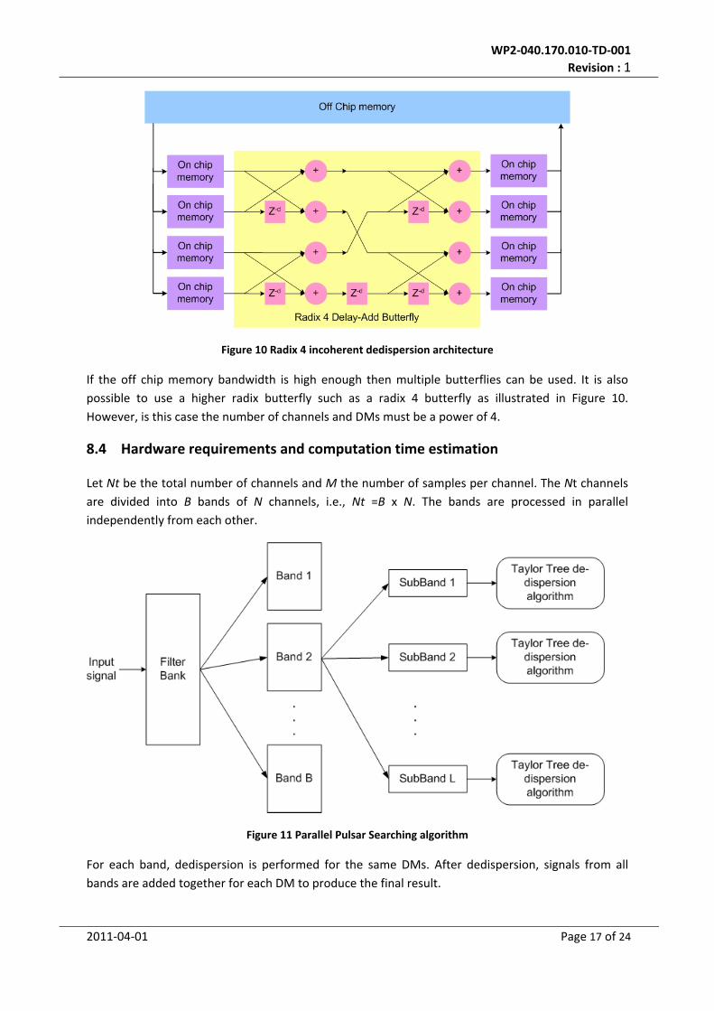
Figure 10 Radix 4 incoherent dedispersion architecture
If the off chip memory bandwidth is high enough then multiple butterflies can be used. It is also
possible to use a higher radix butterfly such as a radix 4 butterfly as illustrated in Figure 10.
However, is this case the number of channels and DMs must be a power of 4.
8.4 Hardware requirements and computation time estimation
Let Nt be the total number of channels and M the number of samples per channel. The Nt channels
are divided into B bands of N channels, i.e., Nt =B x N. The bands are processed in parallel
independently from each other.
Figure 11 Parallel Pulsar Searching algorithm
For each band, dedispersion is performed for the same DMs. After dedispersion, signals from all
bands are added together for each DM to produce the final result.

WP2‐040.170.010‐TD‐001
Revision : 1
2011‐04‐01 Page 18 of 24
The Taylor tree algorithm is used to de‐disperse a band. In order to be able to use this algorithm a
band is divided into small enough sub bands to satisfy the conditions of the algorithm.
Let L be the number of sub bands and K the number of channels per sub band, i.e, N =L x K. The tree
algorithm is applied to each sub band to compute K DMs then the de‐dispersed signals from the L
sub bands are accumulated to produce K DMs for all the band (N channels). The process is repeated
until all the DMs are processed.
To process K DMs, M x K log2(K) samples are read from memory then written back to memory. To
complete the processing of all the sub bands L times more read and write operations are performed,
i.e, M x N log2(K). If a total of D x K DMs are wanted then this will cost D x M x N log2(K) read and
write operations. The accumulation of de‐dispersed signals from each sub band requires reading D x
M x N samples and writing D x M x K.
Therefore, in total, processing one band requires reading D x M x N (1+ log2(K)) samples and writing
D x M (K + N x log2(K)) samples.
Total number of samples to read = D x M x N (1+ log2(K))
Total number of samples to write = D x M (K + N x log2(K))
The number of samples to store input data is N x M. It is also necessary to store a copy of data for
computing K DMs and another to store the final result. In total 2 x N x M + D x K x M/B samples need
to be stored per band.
Total number of samples to store per band = 2 x N x M + D x K x M/B
It is very likely that the external memory will be able to deliver several samples per FPGA clock cycle,
because the memory clock will very likely be a multiple of the FPGA clock, the memory will provide a
double data rate (for DDR) and the memory data width will be a multiple of a sample’s data width.
The number of samples P that can be accessed per FPGA clock cycle is equal to the external memory
bandwidth BWmem divided by the product of the sample’s data width Ws by the FPGA clock
frequency Ffpga.
P = BWmem/(Ws x Ffpga)

WP2‐040.170.010‐TD‐001
Revision : 1
2011‐04‐01 Page 19 of 24
To take advantage of the capabilities of the external memory, data has to be organised in matrix
form where the rows represent sub bands and the columns channels. Each raw would store data of
all channels for one sub band. The data of each channel is stored consecutively and is followed by
the data of the next channel. If the number of sub bands is higher than the maximum number of
rows, then other rows can be stored consecutively by increasing the number of columns. Using this
storage scheme, P samples can be accessed every FPGA clock cycle which allows the use of P parallel
butterfly units to accelerate the processing.
The number of FPGA clock cycles needed to complete the processing of one band NFPGACC is equal
to sum of the total number of samples to read and the total number of samples to write (neglecting
the latency of a butterfly) divided by P. FPGA cycles to process 1 band:
NFPGACC = (D x M x N (1+ log2(K))+ D x M (K + N x log2(K)))/P
After processing each band in parallel, the de‐dispersed signals must be accumulated for each DM.
This requires gathering B x D x K x M samples processing them and storing D x K x M samples.
Gathering these samples from the different parallel systems will take more time than simply reading
data from memory but for the sake of estimation it is approximated as being equal to the memory
access time. Therefore the final total de‐dispersion computation time in clock cycles, TDD can be
expressed as:
TDD = D x M x (N (1+ log2(K))+ (K + N x log2(K)) + (2 B+1) x K)/P =>
TDD = D x M x (Nt x (1+2 x log2(K)) / B+ 2 x (B+1) x K) x (Ws x Ffpga) / BWmem
The final total memory storage requirement is:
TotalExtMemSize = (B x 2 x N x M + D x K x M) x Ws =>
TotalExtMemSize = (2 x Nt x M + D x K x M) x Ws

WP2‐040.170.010‐TD‐001
Revision : 1
2011‐04‐01 Page 20 of 24
If the total number of DMs D x K = Nt then:
TotalExtMemSize = 3 x Nt x M x Ws
The next step in pulsar searching is to perform the FFT of all the signals dispersed at the different
DMs. Each signal has M samples and it is assumed that it will take 2 x M x log2(M) cycles to compute
its FFT. The number of DMs is D x K but they are divided into B sets that can be processed in parallel.
There is also a factor of P reduction in computation time due to the parallelisation permitted by the
external memory bandwidth. This leads to a total FFT computation time TFFT in clock cycles of:
TFFT = 2 x Nt x M x log2(M)/(P x B) =>
TFFT = 2 x Nt x M x log2(M) x (Ws x Ffpga) / (BWmem x B)
The FFT computation does not require any additional memory storage.
For the FPGA resources, it is estimated that P de‐dispersion butterfly units and P FFT butterfly units
can be fitted very easily (P is expected to be <= 1024). Therefore, it is believed that de‐dispersion
and FFT operations can be performed on the same FPGA. The internal memory requirement will
probably not be a problem because the size/depth of the memory is arbitrary and can be reduced if
necessary. However, it is believed that it will not be possible to connect many parallel memory
modules to one FPGA only, therefore it will be necessary to use one FPGA per band.
8.5 Tradeoffs
In order to be able to implement the searching algorithm and run it in ‘real time’, two conditions
must be satisfied:
1. The required hardware must be affordable; 2. The computation time must be faster than or equal to the observation time.
The following is a summary of the formulas that we have developed above to estimate the memory
size and the computation times:
TotalExtMemSize = (2 x Nt x M + D x K x M) x Ws

WP2‐040.170.010‐TD‐001
Revision : 1
2011‐04‐01 Page 21 of 24
TDD = D x M x (Nt x (1+2 x log2(K)) / B+ 2 x (B+1) x K) x (Ws x Ffpga) / BWmem
TFFT = 2 x Nt x M x log2(M) x (Ws x Ffpga) / (BWmem x B)
These formulas are the basis of the following analysis:
The hardware affordability is mainly influenced by the amount of external memory that will be
required to store and process the input data. Reducing the memory size can be achieved by using
the lowest possible number of bits to store the data (Ws). This will also reduce the computation
time. If reducing Ws is not enough then it will be necessary to reduce the number of DMs to
compute, that will reduce D x K, or reduce the signal’s bandwidth, which will reduce Nt x M.
The computation time is not influenced in the same manner as the memory size by the different
parameters. The presence of the log2(K) factor suggests that it is highly desirable to increase K. The
impact of increasing K will be even greater if the number of DMs was equal to the total number of
channels Nt. In this case D x K =Nt, which means increasing K will also reduce D for each of the
subbands.
Figure 12 shows the computation time as a function of D in the case where D x K =Nt. The values of
the other parameters are as follows:
ObservationTime = 600 sec;
SamplingFrequency = 2GHz;
Nt = 8192;
M = (ObservationTime x SamplingFrequency/16)/Nt;
B = 8;
Ffpga = 200MHz;
BWmem = 2 x 64 x 800;
Ws =8 bits. As it can be seen if D>32, i.e. K<256, it will not be possible to perform real time pulsar searching in
this case. The total memory requirement is 210 GB or 26.2 GB per FPGA which might be too high.

WP2‐040.170.010‐TD‐001
Revision : 1
2011‐04‐01 Page 22 of 24
Figure 12 Computation time Vs The total number of sub bands processed using the tree algorithm
The best case scenario is when D = 1 and K =N. In this case, the de‐dispersion computation time is
minimised and more importantly, there is no need to have extra storage for intermediate
computations. The input data can be overwritten because it will not be needed anymore therefore
the memory size requirement drops to:
TotalExtMemSize = Nt x M x Ws
And the computation times becomes:
TDD = M x (Nt x (1+2 x log2(Nt/B)) / B+ 2 x (B+1) x Nt/B) x (Ws x Ffpga) / BWmem
TFFT = 2 x Nt/B x M x log2(M) x (Ws x Ffpga) / (BWmem x B)
Now the memory size is divided by 3 and assuming the same values for the other parameters as
above, the memory requirement is 8.73 GB per FPGA which is more likely to be feasible and
affordable.

WP2‐040.170.010‐TD‐001
Revision : 1
2011‐04‐01 Page 23 of 24
8.6 Mapping a search system into Uniboard
A Uniboard has 8 FPGAs and each one of them has access to two DDR3 banks of 2GB each capable of
800 M transfers/s of 64 bits.
The parameters values that have been used in the previous section match specifically the Uniboard
case. Therefore, for D x K =Nt with D < 64 and:
ObservationTime = 600 sec;
SamplingFrequency = 2GHz;
Nt = 8192;
M = 9.16E6;
Ffpga = 200MHz;
Ws =8 bits.
The memory required per FPGA is 26.2 GB which is higher than the available 4GB. In the second case
where D = 1 and K =N, 8.73 GB per FPGA are required. If Ws is reduced to 4 bits then 4.4 GB per
FPGA will be required and with a 10 % reduction of the signal bandwidth 4 GB per FPGA will be
required. Thus, using one Uniboard it is possible to implement a real time pulsar search engine for a
bandwidth of 900MHz and 1024 DMs.
Another possibility is to use several UNIBOARDS, for example 4 boards, with Ws =4, would be able to
process 1GHz and 8192 DMs.
8.7 Summary and Looking Ahead
We have shown that it is likely possible to coherently dedisperse a full 1 GHz of dual‐polarisation bandwidth, appropriately divided into manageable subbands, with a single Uniboard. The number of subbands required results in a bandwidth per subband which is still large enough to achieve the time resolution desired for the high precision timing experiments. Based on today’s prices a Uniboard in production will cost about 10,000 euros. Given that in SKA phase one we are looking at trying to time a few tens of pulsars simultaneously this should be achievable for something on the order of 250,000 euros. The expected power consumption of 350W per board would then result in a total of about 8kW. Each board would likely need a control PC and the data would also need to be archived.
In the case of the pulsar searching the current Uniboard could likely deal with the expected bandwidth required for the Galactic plane search at a central frequency of about 800 MHz. The bandwidth for that search is likely to be less than that assumed for the calculations above (based more on the 1‐2 GHz range) and by adjusting the number of bits required we could make it possible to dedisperse and search about 500 MHz of bandwidth. A more detailed analysis of the requirements for the Aperture Array search would be required, but the total number of dispersion trials is likely to be similar to the above, and the total data rate less, so it will probably also fit.
Assuming 1GHz beams and a price per Uniboard of 10,000 euros per beam, and considering the number of dispersion trials we can estimate then it will cost about 5 euros per beam per DM. This metric is useful as one of the limiting factors is the number of dispersion measures which needs to be calculated. As above assuming 350W power consumption per board then it will cost 0.17W per beam per DM. However, these estimations are specific to Uniboard and should be considered as upper limits because it is possible that the Uniboard resources and the FPGAs will not be fully utilised.

WP2‐040.170.010‐TD‐001
Revision : 1
2011‐04‐01 Page 24 of 24
It is estimated that something like 4000 beams will be needed in SKA Phase 1 and in this model one Uniboard is needed for each beam. However it may be possible that the increased processing capabilities, and hopefully increased amount of memory on Uniboard 2, or a subsequent board, will improve the efficieny and reduce cost. As noted above it is possible that the capability of the fpgas in Uniboard will not be fully utilised and so a next step would be to consider how we might be able to implement the computationally costly acceleration search as part of this package.