Pseudo-random Simulation of Node Voltages in Medium and …actaenergetica.org/.../1/3/cfde7039_Sobierajski_Pseudo-random_Simu.… · and Low Voltage Grids with Photovoltaic Micro-installations

203

Pseudo-random Simulation of Node Voltages in Medium and Low Voltage Grids with Photovoltaic Micro-installations

AuthorMarian Sobierajski

Keywordslow voltage grid, photovoltaic micro-installations, pseudo-random numbers, statistical analysis

AbstractPower generation by photovoltaic cells depends on random weather conditions, so at the plan-ning stage the active powers output to the grid from photovoltaic micro-installations can be treated as multidimensional random variables with equal probability distribution. Such micro-installations’ passive power outputs depend on the pre-set power factor and therefore should be treated as multidimensional functions of the random active power outputs. Likewise, the received input powers can be treated the same way. Random changes in the output and input powers can be simulated using a pseudo-random number generator. Node voltages corresponding to the random outputs and inputs are derived from the iterative solution of nodal equations for each pseudo-random power balance. The resulting voltages are subjected to statistical analysis. This allows estimating the probability distribution, expected values and standard deviations, and to calculate the probabilities of exceeding the permitted voltage deviations. These considerations will be illustrated by an example calculation.

Marian Sobierajski DOI: 10.12736/issn.2300-3022.2017216

Received: 27.01.2017Accepted: 22.03.2017Available online: 30.06.2017

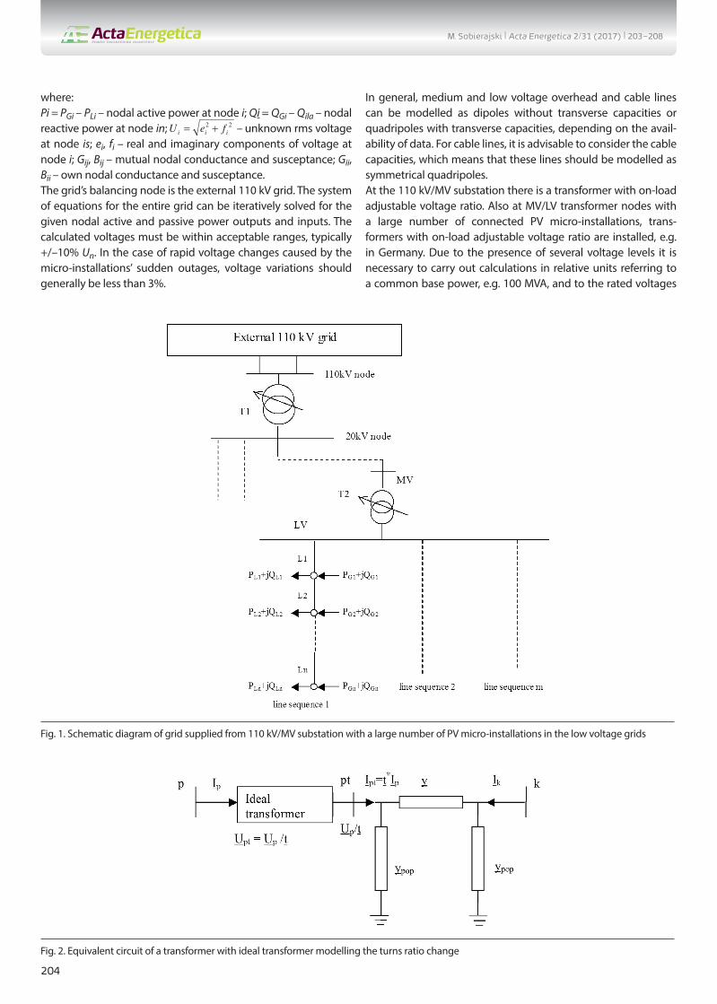
1. IntroductionPhotovoltaic (PV) micro-systems are increasingly connected to low-voltage grids. Fig. 1 shows an example grid supplied from a 110 kV node, where a high number of PV micro-installations are present in the low voltage grids connected to the MV buses. As a result, the power can flow both from the 110 kV node to MV/LV transformers, and the other way around. Consequently, the power flow in the node’s 110 kV/MV transformer can change direction depending on weather conditions. This is so because any node of a low-voltage grid with a high number of PV micro-installations can either input or output power.Photovoltaic cell’s output power depends on random weather conditions. The longer the time ahead of the planned grid opera-tion conditions, the greater the weather forecasts errors and thus the output uncertainty. With pessimistic approach, all values between the minimum and maximum shall be considered as equally probable. It seems reasonable to consider at the plan-ning stage the power outputs to a low-voltage grid as multidi-mensional random variables with equal distribution of prob-ability. Whereas PV micro-installation’s passive power outputs depend on the pre-set power factor. For this reason, they can

be treated as a multidimensional function of the random active power outputs.In a low voltage grid, besides the micro-installations’ output powers, active and passive powers are input and consumed.At the planning stage with a long advance time, the active power inputs can also be treated as multidimensional random variables with equal probability distribution, while the passive power inputs as a function of the multidimensional random vari-able. Normally, the reactive power input should not exceed the permissible power factor tg fi of 0.4.

2. Deterministic power flowThere are non-linear dependencies between nodal powers and voltages resulting from the Ohm and Kirchhoff laws. In the rect-angular system of node voltages, these are square relations

(1)

(2)

M. Sobierajski | Acta Energetica 2/31 (2017) | 203–208

204

where:Pi = PGi – PLi – nodal active power at node i; Qi = QGi – Qila – nodal reactive power at node in; – unknown rms voltage at node is; ei, fi – real and imaginary components of voltage at node i; Gij, Bij – mutual nodal conductance and susceptance; Gii, Bii – own nodal conductance and susceptance.The grid’s balancing node is the external 110 kV grid. The system of equations for the entire grid can be iteratively solved for the given nodal active and passive power outputs and inputs. The calculated voltages must be within acceptable ranges, typically +/–10% Un. In the case of rapid voltage changes caused by the micro-installations’ sudden outages, voltage variations should generally be less than 3%.

In general, medium and low voltage overhead and cable lines can be modelled as dipoles without transverse capacities or quadripoles with transverse capacities, depending on the avail-ability of data. For cable lines, it is advisable to consider the cable capacities, which means that these lines should be modelled as symmetrical quadripoles.At the 110 kV/MV substation there is a transformer with on-load adjustable voltage ratio. Also at MV/LV transformer nodes with a large number of connected PV micro-installations, trans-formers with on-load adjustable voltage ratio are installed, e.g. in Germany. Due to the presence of several voltage levels it is necessary to carry out calculations in relative units referring to a common base power, e.g. 100 MVA, and to the rated voltages

Fig. 1. Schematic diagram of grid supplied from 110 kV/MV substation with a large number of PV micro-installations in the low voltage grids

Fig. 2. Equivalent circuit of a transformer with ideal transformer modelling the turns ratio change


205

of each network. The impact of turns ratio change on the trans-former’s equivalent parameters is considered by introducing to its equivalent circuit on the initial node side an ideal transformer with variable voltage ratio t, as shown in Fig. 2.Idle transformer’s voltage ratio in relative units is equal to the ratio of its rated voltages expressed in relative units:

(3)

Where the transformer voltage ratio is on-load adjustable:

(4)

where: transformer’s actual turns ratio, after tap change

on the upper voltage side at node p.Transformer’s ratio change alters its complex impedances (admit-tances). If a transformer’s longitudinal impedance in relative units on the side of node k is:

(5)

then on the side of node p it depends on the transformer’s actual voltage ratio:

(6)

In the admittance terms:

(7)

(8)

In the case of transverse parameters, the admittance in relative units is, respectively:

(9)

(10)

Taking into account the impact of the voltage ratio change on the transformer parameters in relative computer calculations requires introducing the transformer’s equivalent circuit shown in Fig. 3.Complex own admittances of the nodes of the quadripole model-ling a transformer with adjustable voltage ratio are:

(11)

(12)

Complex mutual admittances of the quadripole’s nodes are equal:

(13)

It should be noted that changing a transformer’s ratio alters the complex own and mutual admittances in the grid nodes connected to the transformer’s beginning and end nodes. This fact must be taken into account when iteratively solving the system of power flow nodal equations (1, 2).

3. Power flow model with random nodal power changesAt any node of the grid supplied from the 110 kV/MV substa-tion the power can be either input or output within the range between the minimum and maximum. For power output:

(14)

Reactive power results from the active power output and the pre-set power factor tgφ

Fig. 3. Equivalent circuit of a transformer with adjustable voltage ratio


206

(15)

Likewise, the input active powers result from the maximum and minimum demand:

(16)

Nodal load’s reactive power input results from its power factor:

(17)

It can be assumed at the planning stage that each active power is equally likely in the range from the minimum to maximum, i.e. the active power is subject to a rectangular probability distribu-tion within the range. With MATLAB random numbers can be generated, which are subject to rectangular probability distribu-tion in range [0,1]. For this purpose, the rand feature is used. To generate a pseudo-random number with rectangular probability interval in range [a, b] the following formula should be used:

x = a + (b - a)rand (18)

With the application of formula (18) for the output and input nodal powers the following dependencies are obtained:• power output at node from PV micro-installation

Pg. = PMing + (PGmax – PGmin)rand (19)

(20)

• power input at node

PL = PLmin + (PLmax – PLmin)rand (21)

(22)

Determination of empirical cumulative distribution function requires an increasing sorting of the voltages at a given node. The resulting is a sample of nsym incrementally sorted simulations:

(Y1, Y2, ..., Ynsym) (23)

The empirical cumulative distribution function is defined by formula:

(24)

where: – number of elements satisfying the inequality

(25)

Empirical cumulative distribution function Fe(y) is uniform across intervals and jumps by 1/nsym in points yi. It is a statistical approximation of the unknown theoretical distribution function and is similar in shape. The larger the number nsym of simula-tions, the better the empirical distribution function approximates

the theoretical distribution function. With its values known, the empirical distribution function can be approximated by n-th degree polynomial function. This produces a continuous func-tion describing the empirical distribution. For this purpose, first, we standardise random variable:

– average (26)

– standard deviation (27)

– standardised random variable (28)

(29)

(30)

(31)

Then we approximate the empirical distribution function by n-th degree polynomial:

(32)

A function that describes the empirical distribution function must be a non-decreasing function, which meets with a pre-set accuracy the following restrictions:

(33)

After finding the polynomial that approximates the empirical distribution function, the probability can be estimated of such an event that the angle offset does not exceed the permissible value:

(34)

4. Power flow simulation in an exemplary power grid with photovoltaic micro-installationsThe diagram of the grid is shown in Fig. 1. Short circuit power of the external system is 1,500 MVA. Transformer T1 with adjust-able voltage ratio has the following parameters: SN = 40 MVA; UNH = 115 kV +/–16%, +/–12 adjustment steps; UNL = 22 kV; uk = 11%; Pcu = 205 kW; PFe = 33 kW; I0 = 0.5%. The 20 kV AFL6 70 line’s equivalent parameters are: R = 4 Ω, X = 3,6 Ω, B = 32 μS. The low voltage grid is connected by a medium voltage line and adjustable ratio transformer T2 with the following parameters: SN = 100 kVA; UNH = 21 kV +/–10%, +/–8 adjustment steps; UNL = 0.42 kV; uk = 4.5%; Pcu = 1.7 kW; PFe = 0.22 kW; I0 = 2%. The LV line consists of 9 AFL 70 mm2 sections, each 100 m long (Rsection = 0,0436 Ω, Xsection = 0.0309 Ω).Aggregate power input from the substation’s 20 kV buses is (5 + j2) MVA. Power inputs and outputs in the LV grid’s nodes are characterized by the minimum and maximum active powers and power factors: PGmin = 1 kW, PGmax = 10 kW, tgφ = –0.3, PLmin = 1 kW, PLmax = 2 kW, tgφ = 0.4.


207

Two variants of the grid operation with PV micro-installations were analysed. The results are presented in Tab. 1.T1 adjustment option – T1 transformer ratio adjustment maintains 1.05 Un voltage on the MV side, no T2 transformer adjustment.T1T2 adjustment option – T1 transformer ratio adjustment main-tains 1.05 Un voltage on the MV side, and at the same time T2 transformer ratio adjustment maintains Un voltage on the LV side.Random voltage changes are shown in Fig. 4 and Fig. 5, while Umin = mU – 3sU, Umax = mU + 3sU. It can be seen that in the grid operation option without the MV/LV transformer ratio adjust-ment the permissible grid voltage levels are violated. MV/LV transformer voltage ratio adjustment prevents such voltage level violations due to grid voltages’ random changes.

5. SummaryPower generation by photovoltaic cells depends on random weather conditions, so at the planning stage the active powers output to the grid from photovoltaic micro-installations can be treated as multidimensional random variables with equal prob-ability distribution.

Fig. 4. Random voltage changes in grid with photovoltaic micro-instal-lations exceed the permissible voltage Udopmax = 1.1 Un

Fig. 5. MV/LV transformer voltage ratio adjustment prevents excesses over the permissible voltage Udopmax = 1.1 Un in grid

Tab. 1. Power flow simulation results: mU – expected value, sU – stan-dard deviation, Udopmin, Udopmax – allowable minimum and maximum grid voltages, p {Udopmin < U < Udopmax} – probability of random voltage changes remaining within the permissible range

Node No. Name Option mU sU Udopmin Udopmax

p{Udopmin < U <

Udopmax}

1 Power system

T1 adjustment 1.1 0 0.9 1.1 1

T1T2 adjustment 1.1 0 0.9 1.1 1

2 110 kV node

T1 adjustment 1.0985 0 0.9 1.1 1

T1T2 adjustment 1.0985 0 0.9 1.1 1

3 20 kV node

T1 adjustment 1.0589 0 0.9 1.1 1

T1T2 adjustment 1.0589 0 0.9 1.1 1

4 MV T1T2 adjustment 1.0592 0.0001 0.9 1.1 1

T1T2 adjustment 1.0589 0.0001 0.9 1.1 1

5 LV T1 adjustment 1.0632 0.0012 0.9 1.1 1

T1T2 adjustment 1.0011 0.0013 0.9 1.1 1

6 wL1 T1 adjustment 1.0716 0.0031 0.9 1.1 1

T1T2 adjustment 1.0098 0.0033 0.9 1.1 1

7 wL2 T1 adjustment 1.0789 0.0047 0.9 1.1 1

T1T2 adjustment 1.0176 0.0051 0.9 1.1 1

8 wL3 T1 adjustment 1.0853 0.0062 0.9 1.1 0.99

T1T2 adjustment 1.0243 0.0067 0.9 1.1 1

9 wL4 T1 adjustment 1.0909 0.0076 0.9 1.1 0.89

T1T2 adjustment 1.0301 0.0082 0.9 1.1 1

10 wL5 T1 adjustment 1.0954 0.0087 0.9 1.1 0.7

T1T2 adjustment 1.0349 0.0094 0.9 1.1 1

11 wL6 T1 adjustment 1.099 0.0097 0.9 1.1 0.54

T1T2 adjustment 1.0386 0.0105 0.9 1.1 1

12 wL7 T1 adjustment 1.1017 0.0105 0.9 1.1 0.44

T1T2 adjustment 1.0415 0.0114 0.9 1.1 1

13 wL8 T1 adjustment 1.1034 0.0111 0.9 1.1 0.38

T1T2 adjustment 1.0434 0.012 0.9 1.1 1

14 wL9 T1 adjustment 1.1043 0.0114 0.9 1.1 0.35

T1T2 adjustment 1.0443 0.0124 0.9 1.1 1


208

Micro-installations’ passive power outputs depend on a pre-set power factor and therefore should be treated as functions of the random active power outputs.In a low voltage grid, besides the micro-installations’ output powers, active and passive powers are input and consumed. At the planning stage, the input powers, as well as the output powers, can also be treated as a multidimensional random vari-able with equal probability distribution.Random changes in the vector of nodal powers in the grid can be simulated using a pseudo-random number generator. After the voltage-nodes equations’ iterative solution, random voltages are obtained in the grid’s individual nodes.After statistical analysis, the empirical cumulative distribution of the voltage probability in any node of the grid is obtained, which

makes it possible to estimate the probability of random voltages remaining in the permissible range.MV/LV transformer voltage ratio adjustment allows preventing the random voltage’s excesses over the permissible grid voltages.

REFERENCES

1. Z. Kremens, M. Sobierajski, “Analiza systemów elektroenergetycznych” [Analysis of power systems], WNT, Warsaw 1996.

2. A. Plucińska, E. Pluciński, “Rachunek prawdopodobieństwa. Statystyka matematyczna. Procesy stochastyczne” [Probability calcu-lus. Mathematical statistics. Stochastic processes], WNT, Warsaw 2000.

Marian SobierajskiWrocław University of Technology

e-mail: [email protected]

Prof. Sobierajski deals with scientific issues related to planning and controlling power systems. His works mainly refer to probabilistic power flows, voltage stability

and electricity quality, and to interoperation of distributed sources with transmission grids. He has recently studied smart power grids, interoperation of photovoltaic

micro-installations and small systems with medium and low voltage distribution grids and frequency control during island operation.


209

PL

Pseudolosowa symulacja napięć węzłowych w sieci średniego i niskiego napięcia z fotowoltaicznymi mikroinstalacjami

Autor Marian Sobierajski

Słowa kluczowesieć niskiego napięcia, mikroinstalacje fotowoltaiczne, liczby pseudolosowe, analiza statystyczna

StreszczenieWytwarzanie mocy przez ogniwa fotowoltaiczne zależy od losowych warunków pogodowych, dlatego na etapie planowania moce czynne wprowadzane do sieci przez mikroinstalacje fotowoltaiczne mogą być traktowane jako wielowymiarowa zmienna losowa o równomiernym rozkładzie prawdopodobieństwa. Natomiast wytwarzane moce bierne mikroinstalacji zależą od zadanego współ-czynnika mocy i dlatego powinny być traktowane jako wielowymiarowa funkcja losowych wytwarzanych mocy czynnych. Podobnie mogą być traktowane moce odbierane. Losowe zmiany mocy generowanych i odbieranych mogą być symulowane z wykorzysta-niem generatora liczb pseudolosowych. Napięcia węzłowe odpowiadające losowym generacjom i odbiorom wynikają z iteracyjnego rozwiązania równań węzłowych dla każdej pseudolosowej realizacji bilansów mocy. Otrzymane wartości napięć poddane są analizie statystycznej. Pozwala to oszacować rozkład prawdopodobieństwa, wartości oczekiwane i odchylenia standardowe oraz wyliczyć prawdopodobieństwa przekroczenia dopuszczalnych odchyleń napięć. Rozważania zostaną zilustrowane przykładem obliczeniowym.

Data wpływu do redakcji: 27.01.2017Data akceptacji artykułu: 22.03.2017Data publikacji online: 30.06.2017

1. WprowadzenieDo sieci niskiego napięcia coraz częściej przyłączane są mikroinstalacje fotowolta-iczne (PV). Na rys. 1 pokazano przykła-dową sieć zasilaną z GPZ 110 kV, w której w poszczególnych sieciach niskiego napięcia, połączonych z magistralami SN, występuje duża liczba mikroinstalacji PV. W rezultacie moc może płynąć zarówno z GPZ do punktów transformatorowych SN/nN, jak i odwrotnie. W konsekwencji moc w transformatorze w GPZ 110 kV/SN może zmieniać kierunek, zależnie od warunków pogodowych. Dzieje się tak, ponieważ w dowolnym węźle sieci niskiego napięcia z dużą liczbą mikroinstalacji może wystąpić zarówno moc odbierana, jak i generowana. Moc wytwarzana przez ogniwa fotowol-taiczne zależy od losowych warunków pogodowych. Im dłuższy okres czasu wyprzedzający planowane warunki pracy sieci, tym większe błędy prognoz pogodo-wych i tym większa niepewność generacji. Pesymistyczne podejście nakazuje rozważać jako jednakowo prawdopodobne wartości między minimalną i maksymalną wartością. Zasadne wydaje się traktowanie na etapie planowania generowanych mocy w sieci niskiego napięcia jako wielowymiarowej zmiennej losowej o równomiernym rozkła-dzie prawdopodobieństwa. Natomiast moce bierne wytwarzane przez mikroinstalacje zależą od zadanego współczynnika mocy. Z tego powodu mogą być traktowane jako wielowymiarowa funkcja losowych wytwa-rzanych mocy czynnych.W sieci niskiego napięcia, obok mocy wytwarzanych przez mikroinstalacje, wystę-pują pobory mocy czynnych i biernych. Na etapie planowania z dużym okresem wyprzedzenia moce czynne odbierane mogą być również traktowane jako wielowymia-rowe zmienne losowe o równomiernym

rozkładzie prawdopodobieństwa, natomiast moce bierne odbierane jako funkcja wielo-wymiarowej zmiennej losowej. Zwykle pobór mocy biernej nie powinien przekra-czać dopuszczalnego tangensa mocy 0,4.

2. Deterministyczny rozpływ mocyMiędzy mocami i napięciami węzłowymi występują nieliniowe zależności wynikające z praw Ohma i Kirchhoffa. W układzie skła-dowych prostokątnych napięć węzłowych są to zależności kwadratowe

(1)

(2)

gdzie: Pi = PGi – PLi – węzłowa moc czynna w węźle i; Qi = QGi – QLi – węzłowa moc i bierna

w węźle i; – nieznana wartość skuteczna napięcia w węźle i; ei, fi – składowa rzeczywista i urojona napięcia w węźle i; Gij, Bij – konduktancja i susceptancja węzłowa wzajemna; Gii, Bii – konduktancja i suscep-tancja węzłowa własna.

Węzłem bilansującym sieci jest sieć zewnętrzna 110 kV. Układ równań dla całej sieci może być rozwiązany iteracyjnie dla zadanych węzłowych mocy czynnych i biernych generowanych oraz odbiera-nych. Wyliczone napięcia muszą się mieścić w dopuszczalnych przedziałach, zwykle +/–10% Un. W przypadku szybkich zmian napięć powodowanych nagłym wyłączeniem

mikroinstalacji zmiany napięć powinny być na ogół mniejsze od 3%.W ogólności linie napowietrzne i kablowe średniego oraz niskiego napięcia mogą być modelowane w postaci dwójników bez pojemności poprzecznych lub czwórników z pojemnościami poprzecznymi, zależnie od dostępności danych. W przypadku linii kablowych wskazane jest uwzględnienie pojemności kabli, co oznacza, że linie te powinny być modelowane w postaci syme-trycznych czwórników.W stacji GPZ 110 kV/SN występuje trans-formator z regulowaną przekładnią pod obciążeniem. Również w punktach trans-formatorowych SN/nN z dużą liczbą przy-łączonych mikroinstalacji instaluje się transformatory z regulowaną przekładnią pod obciążeniem, np. w Niemczech. Ze względu na występowanie kilku poziomów napięć konieczne jest prowadzenie obliczeń w jednostkach względnych odniesionych do wspólnej mocy bazowej, np. 100 MVA, oraz do napięć znamionowych poszczegól-nych sieci. Uwzględnienie wpływu zmiany przekładni zwojowej na parametry zastępcze transformatora uzyskuje się, wprowa-dzając do schematu zastępczego po stronie węzła początkowego idealny transformator o zmiennej przekładni t, rys. 2.Przekładnia w jednostkach względnych nieobciążonego transformatora jest równa stosunkowi napięć znamionowych trans-formatora wyrażonych w jednostkach względnych:

(3)

This is a supporting translation of the original text published in this issue of “Acta Energetica” on pages 203–208. When referring to the article please refer to the original text.

M. Sobierajski | Acta Energetica 2/31 (2017) | translation 203–208

210

PL

W przypadku, gdy przekładnia transfor-matora jest regulowana pod obciążeniem, mamy:

(4)

gdzie:

– aktualna przekładnia zwojowa transformatora, po zmianie zaczepu od strony górnego napięcia w węźle p.Zmiana przekładni transformatora powo-duje zmianę zespolonych impedancji (admi-tancji) transformatora. Jeżeli impedancja podłużna transformatora w jednostkach względnych po stronie węzła k wynosi:

(5)

to po stronie węzła p zależy od aktualnej wartości przekładni transformatora:

(6)

W zapisie admitancyjnym mamy:

(7)

(8)

W przypadku parametrów poprzecznych admitancja w jednostkach względnych wynosi odpowiednio:

(9)

(10)

Uwzględnienie wpływu zmiany przekładni na parametry transformatora w jednostkach względnych w obliczeniach komputerowych wymaga wprowadzenia schematu zastęp-czego transformatora pokazanego na rys. 3.Zespolone admitancje własne węzłów czwórnika modelującego transformator z regulowaną przekładnią wynoszą:

(11)

(12)

Zespolone admitancje wzajemne węzłów tego czwórnika są sobie równe:

(13)

Należy zauważyć, że zmiana przekładni transformatora powoduje zmianę zespo-lonych admitancji własnych i wzajemnych w węzłach sieci łączących się węzłami początku oraz końca transformatora. Fakt ten musi być uwzględniony w trakcie itera-cyjnego rozwiązywania układu równań węzłowych rozpływu mocy (1, 2).

3. Model rozpływu mocy z losowymi zmianami mocy węzłowychW dowolnym węźle badanej sieci zasilanej z GPZ 110 kV/SN mogą wystąpić zarówno odbierane, jak i generowane moce w prze-działach od minimalnej do maksymalnej wartości. W przypadku generacji mamy:

(14)

Moc bierna wynika z wartości generowanej mocy czynnej i zadanego tangensa mocy:

(15)

Podobnie moce czynne odbierane wyni-kają z maksymalnego i minimalnego zapotrzebowania:

(16)

Moc bierna odbioru węzłowego wynika z tangensa mocy odbiorników:

(17)

Na etapie planowania można przyjąć, że każda z wartości mocy czynnej jest jedna-kowo prawdopodobna w przedziale od min. do max., czyli moc czynna podlega prosto-kątnemu rozkładowi prawdopodobieństwa w przedziale od min. do max.MATLAB pozwala generować liczby losowe, podlegające prostokątnemu rozkładowi prawdopodobieństwa w przedziale [0,1]. W tym celu wykorzystuje się funkcję rand. W celu wygenerowania liczby pseudolo-sowej o prostokątnym przedziale prawdopo-dobieństwo w przedziale [a, b] należy zasto-sować formułę:

x = a + (b – a)rand (18)

Zastosowanie formuły (18) dla mocy węzłowych generowanych i odbieranych daje następujące zależności:• moc generowana w węźle przez mikroin-

stalcję PV

PG = PGmin + (PGmax – PGmin)rand (19)

(20)

• moc odbierana w węźle

PL = PLmin + (PLmax – PLmin)rand (21)

(22)

Rys. 1. Schemat sieci zasilanej z GPZ 110 kV/SN z dużą liczbą mikroinstalacji w sieciach niskiego napięcia

Rys. 2. Schemat zastępczy transformatora z idealnym transformatorem modelującym zmianę przekładni zwojowej



211

PL

Wyznaczenie dystrybuanty empirycznej wymaga rosnącego posortowania realizacji napięcia w danym węźle. W konsekwencji otrzymujemy próbę składającą się z liczby nsym posortowanych rosnąco symulacji:

(Y1, Y2, ..., Ynsym) (23)

Dystrybuanta empiryczna jest funkcją okre-śloną wzorem:

(24)

gdzie:

– liczba elementów spełniają-cych nierówność (25)

Dystrybuanta empiryczna Fe(y) jest prze-działami stała i ma skoki o wartości 1/nsym w punktach yi. Jest statystycznym przybliże-niem nieznanej dystrybuanty teoretycznej i ma zbliżony do niej kształt. Im większa liczba symulacji nsym, tym dystrybuanta empiryczna stanowi lepsze przybliżenie dystrybuanty teoretycznej.Mając wartości dystrybuanty empirycznej, możemy ją aproksymować wielomianem n-tego stopnia. Uzyskujemy w ten sposób ciągłą funkcję opisującą dystrybuantę empi-ryczną. W tym celu dokonujemy najpierw standaryzacji zmiennej losowej

– średnia (26)

– odchylenie standardowe (27)

– zmienna losowa standaryzowana (28)

(29)

(30)

(31)

Następnie dokonujemy aproksymacji dystrybuanty empirycznej wielomianem n-tego stopnia:

(32)

Funkcja opisująca dystrybuantę empi-ryczną musi być funkcją niemalejącą, speł-niającą z zadaną dokładnością następujące ograniczenia:

(33)

Po znalezieniu wielomianu aproksymu-jącego dystrybuantę empiryczną można oszacować prawdopodobieństwo zdarzenia, że rozchył kątowy nie przekroczy dopusz-czalnej wartości:

(34)

Rys. 3. Schemat zastępczy transformatora z regulowaną przekładnią

Rys. 4. Losowe zmiany napięcia w sieci z mikroinstalacjami fotowoltaicznymi przekraczają dopuszczalny poziom napięcia Udopmax = 1,1 Un

Rys. 5. Zastosowanie regulacji przekładni transformatora SN/nN zapobiega przekroczeniu dopuszczalnego poziomu napięcia Udopmax = 1,1 Un w sieci



212

PL

4. Symulacja rozpływów mocy w przykładowej sieci elektroenergetycznej z mikroinstalacjami fotowoltaicznymiSchemat analizowanej sieci poka-zano na rys. 1. Moc zwarciowa systemu zewnętrznego wynosi 1500 MVA. Transformator T1 z regulowaną prze-kładnią ma następujące parametry: SN = 40 MVA; UNH = 115 kV +/– 16%, +/–12 stopni regulacyjnych; UNL = 22 kV; uk = 11%; Pcu = 205 kW; PFe = 33 kW; I0 = 0,5%. Parametr y zastępcze linii 20 kV AFL6 70 są następujące: R = 4 Ω, X = 3,6 Ω, B = 32 . Sieć niskiego napięcia jest połączona linią średniego napięcia za pomocą transformatora T2 z regulowaną przekładnią o nastę-pujących parametrach: SN = 100 kVA; UNH = 21 kV +/– 10%, +/–8 stopni regulacyj-nych; UNL = 0,42 kV; uk = 4,5%; Pcu = 1,7 kW;

PFe = 0,22 kW; I0 = 2%. Linia nN składa się z 9 odcinków AFL 70 mm2, po 100 m każdy (Rodcinka = 0,0436 Ω, Xodcinka = 0,0309 Ω). Sumaryczny odbiór z szyn 20 kV GPZ wynosi (5 + j2) MVA. Odbiory i gene-racje w węzłach sieci nN scharaktery-zowane są przez minimalne i maksy-malne moce czynne oraz tangensy mocy: PGmin = 1 kW, PGmax = 10 kW, tgφ = –0,3, PLmin = 1 kW, PLmax = 2 kW, tgφ = 0,4.Analizie poddano dwa warianty pracy sieci z mikroinstalacjami. Wyniki zestawiono w tab. 1.• Wariant reg.T1 – układ regulacji prze-

kładni transformatora T1 utrzymuje napięcie 1,05 Un po stronie SN, brak regu-lacji przekładni transformatora T2.

• Wariant reg.T1T2 – układ regulacji przekładni transformatora T1 utrzy-muje napięcie 1,05 Un po stronie SN

i jednocześnie układ regulacji przekładni transformatora T2 utrzymuje napięcie Un po stronie nN.

Losowe zmiany napięcia przedstawiono na rys. 4 i 5, przy czym Umin = mU – 3sU, Umax = mU + 3sU. Widać, że w wariancie pracy sieci bez regulacji przekładni trans-formatora SN/nN w sieci naruszone zostają dopuszczalne poziomy napięcia. Zastosowanie regulacji przekładni napięcia w transformatorze SN/nN zapobiega takiemu naruszeniu dopuszczalnych poziomów napięcia przez losowe zmiany napięć w sieci.

5. PodsumowanieWytwarzanie mocy przez ogniwa foto-woltaiczne zależy od losowych warunków pogodowych, dlatego na etapie planowania moce czynne wprowadzane do sieci przez mikroinstalacje fotowoltaiczne mogą być traktowane jako zmienne losowe o równo-miernym rozkładzie prawdopodobieństwa.Wytwarzane moce bierne mikroinstalacji zależą od zadanego współczynnika mocy i dlatego powinny być traktowane jako funkcje losowych wytwarzanych mocy czynnych.W sieci niskiego napięcia, obok mocy wytwarzanych przez mikroinstalacje, występują pobory mocy czynnych i bier-nych. Na etapie planowania moce odbie-rane, podobnie jak wytwarzane, mogą być również traktowane jako wielowymiarowa zmienna losowa o równomiernym rozkła-dzie prawdopodobieństwa.Losowe zmiany wektora mocy węzłowych w sieci mogą być symulowane z wykorzy-staniem generatora liczb pseudolosowych. Po iteracyjnym rozwiązaniu równań napię-ciowo-węzłowych otrzymuje się losowe realizacje napięć w poszczególnych węzłach sieci.Po przeprowadzeniu analizy statystycznej otrzymuje się empiryczną dystrybuantę prawdopodobieństwa napięcia w dowolnym węźle sieci, co pozwala oszacować praw-dopodobieństwo pozostawania losowych zmian napięcia w dopuszczalnym przedziale.Zastosowanie regulacji przekładni transfor-matora SN/nN pozwala zapobiegać przekro-czeniu przez losowe napięcia dopuszczal-nych poziomów napięć w sieci.

Bibliografia

1. Kremens Z., Sobierajski M., Analiza systemów elektroenergetycznych, WNT, Warszawa 1996.

2. Plucińska A., Pluciński E., Rachunek prawdopodobieństwa. Statystyka mate-matyczna. Procesy stochastyczne, WNT, Warszawa 2000.

Tab. 1. Wyniki symulacji rozpływów mocy: mU – wartość oczekiwana, sU – odchylenie standardowe, Udopmin, Udopmax – dopuszczalny minimalny i maksymalny poziom napięcia w sieci, p {Udopmin < U < Udopmax} – prawdopodo-bieństwo pozostawania losowych zmian napięcia w dopuszczalnym przedziale

Nr węzła Nazwa Wariant mU sU Udopmin Udopmaxp {Udopmin < U < Udopmax}

1 SEE reg. T1 1,1 0 0,9 1,1 1

reg. T1T2 1,1 0 0,9 1,1 1

2 GPZ110kV reg. T1 1,0985 0 0,9 1,1 1

reg. T1T2 1,0985 0 0,9 1,1 1

3 GPZ20kV reg. T1 1,0589 0 0,9 1,1 1

reg. T1T2 1,0589 0 0,9 1,1 1

4 SN reg. T1 1,0592 0,0001 0,9 1,1 1

reg. T1T2 1,0589 0,0001 0,9 1,1 1

5 nN reg. T1 1,0632 0,0012 0,9 1,1 1

reg. T1T2 1,0011 0,0013 0,9 1,1 1

6 wL1 reg. T1 1,0716 0,0031 0,9 1,1 1

reg. T1T2 1,0098 0,0033 0,9 1,1 1

7 wL2 reg. T1 1,0789 0,0047 0,9 1,1 1

reg. T1T2 1,0176 0,0051 0,9 1,1 1

8 wL3 reg. T1 1,0853 0,0062 0,9 1,1 0,99

reg. T1T2 1,0243 0,0067 0,9 1,1 1

9 wL4 reg. T1 1,0909 0,0076 0,9 1,1 0,89

reg. T1T2 1,0301 0,0082 0,9 1,1 1

10 wL5 reg. T1 1,0954 0,0087 0,9 1,1 0,7

reg. T1T2 1,0349 0,0094 0,9 1,1 1

11 wL6 reg.T1 1,099 0,0097 0,9 1,1 0,54

reg. T1T2 1,0386 0,0105 0,9 1,1 1

12 wL7 reg. T1 1,1017 0,0105 0,9 1,1 0,44

reg. T1T2 1,0415 0,0114 0,9 1,1 1

13 wL8 reg. T1 1,1034 0,0111 0,9 1,1 0,38

reg. T1T2 1,0434 0,012 0,9 1,1 1

14 wL9 reg. T1 1,1043 0,0114 0,9 1,1 0,35

reg. T1T2 1,0443 0,0124 0,9 1,1 1

Marian Sobierajskiprof. dr hab. inż. Politechnika Wrocławskae-mail: [email protected] się problemami naukowymi związanymi z planowaniem i sterowaniem systemów elektroenergetycznych. Jego prace dotyczą głównie probabilistycz-nych rozpływów mocy, stabilności napięciowej i jakości energii elektrycznej oraz współpracy rozproszonych źródeł z sieciami przesyłowymi. Ostatnie badania związane są z inteligentnymi sieciami elektroenergetycznymi, współpracą mikroinstalacji i małych instalacji fotowoltaicznych z sieciami dystrybucyjnymi średniego i niskiego napięcia oraz regulacją częstotliwości w czasie pracy wyspowej.



213

Energy Storage Control Strategy in a Prosumer System and its Impact on the Distribution Grid

AuthorsPrzemysław UrbanekIrena WasiakRyszard Pawełek

Keywordsmicrosystem, prosumer installation, prosumer, electricity storage, energy storage control, electric power quality

AbstractThis paper discusses the operation of a low voltage prosumer system consisting of receivers and power sources. The system represents a hypothetical customer with variable energy input and output. The main technical issues related to the operation of such a system are presented. The application of an electric energy storage in the system for the purpose of managing the active power and providing the ancillary services relevant for the system’s owner is discussed. The basic criterion of the system’s performance is maximizing the use of the energy generated by the prosumer and maintaining the power factor at a desired level. The storage efficiency was tested using a simulation model developed in the PSCAD / EMTDC program. Sample simulation results are presented.

DOI: 10.12736/issn.2300-3022.2017217

Received: 14.02.2017Accepted: 07.03.2017Available online: 30.06.2017

1. IntroductionThe continuous development of electricity generation technolo-gies, and the ability to increase supply reliability and reduce electricity costs have prompted citizens to have their own power plants. Consumers have begun to equip their home installa-tions with distributed sources of electricity, especially renewable energy sources (RES), using free energy from the sun and wind. It can be predicted that with decreasing prices of such sources this trend will continue.The European Union’s climate regulations and policy required the Polish legislators to introduce the definition of a prosumer. According to the Renewable Energy Act [14], a prosumer is an individual, who generates electricity for their own needs, which means the simultaneous generation and consumption of energy. The energy produced in the sources is consumed in the receivers and its surplus is sold to the power grid. In the oppo-site situation, when the local source output is less than demand, the missing energy is bought from a power company. In the light of the present law, a prosumer is therefore a recipient of electricity, who is allocated an appropriate tariff and, according

to it, settles their accounts for the purchased/sold energy. The Act [14] sets out rules for the sale of electricity in such a way that a prosumer has the option to free of charge input from the grid 80% of the surplus energy output to it. A prosumer is not an electricity generator, and this condition obliges the prosumer to comply with the terms and conditions of the elec-tricity distribution contract [12, 13] regarding reactive power. Under these terms and conditions, the prosumer may consume reactive power up to the value resulting from the established tg φ coefficient.Electricity generation from one’s own source reduces the active power input from the distribution grid. At the same time, the consumption of passive power remains unchanged, because the energy sources usually operate with power factor cos φ = 1. Consequently, tg φ increases at the prosumer system’s inter-connection with the distribution grid. For any excess over tg φ = 0.4 the power company shall charge a penalty [10, 11]. As a consequence, the prosumer’s investment in, for example, a wind turbine does not produce the expected savings and, in an extreme case, can cause losses [2].

P. Urbanek et al. | Acta Energetica 2/31 (2017) | 213–221

Documents

Pseudo-random Simulation of Node Voltages in Medium and …actaenergetica.org/.../1/3/cfde7039_Sobierajski_Pseudo-random_Simu.… · and Low Voltage Grids with Photovoltaic Micro-installations