Embed Size (px)
Citation preview

Pruning to improve spatial complementarity in utilization of below-ground resources
Department for International Development
Forestry Research Programme - Final Technical Report Project R7342
J. Wilson, J.D. Deans, D.C. Mobbs, A-M. Giacomello & N. Hall, CEH, Edinburgh and Wallingford UK C.K. Ong, T. Raussen & A. Teklerbehan Tefera, ICRAF, Nairobi and Uganda T-N. Wajja-Musukwe, B.D. Sande & D. Siriri, FORRI Uganda D.W. Odee, J.M. Mulatya and E. Kiptot, KEFRI, Kenya

Pruning to improve spatial complementarity in utilization of below-ground resources
Department for International Development
Forestry Research Programme - Final Technical Report Project R7342
Reporting period: 1st October 1998 – 31st July 2003
J. Wilson, J.D. Deans, D.C. Mobbs, A-M. Giacomello & N. Hall, CEH, Edinburgh1 and Wallingford2 UK C.K. Ong, T. Raussen & A. Tefera Teklerbehan, ICRAF3, Nairobi and Uganda N. Wajja-Musukwe, B.D. Sande & D. Siriri, FORRI, Kampala4 and Kabale5, Uganda D. Odee, J. Mulatya and E. Kiptot, KEFRI6, Kenya This publication is an output from a research project partly funded by the United Kingdom Department for International Development (DFID) for the benefit of developing countries. The views expressed are not necessarily those of DFID. R7342 Forestry Research Programme.
1 Centre for Ecology and Hydrology, Bush Estate, Penicuik, Midlothian EH26 0QB, UK. 2 Centre for Ecology and Hydrology, Crowmarsh Gifford, Wallingford, Oxfordshire OX10 8BB, UK. 3 World Agroforestry Centre (ICRAF), United Nations Avenue, Gigiri, PO Box 30677, Nairobi, Kenya 4 National Agricultural Research Organisation, Forestry Resources Research Institute, PO Box 1752, Kampala, Uganda 5 AFRENA-Uganda Project, PO Box 311, Kabale, Uganda 6 Kenya Forestry Research Institute (KEFRI), PO Box 20412, Nairobi, Kenya.

i
Executive Summary Competition between trees and crops is a problem in many agroforestry systems as trees get older. As well as casting shade, trees also compete below-ground for water and nutrients, causing much of the reduction in crop growth close to trees. Studies in Kenya and Uganda tested simple management (crown and root pruning) techniques for reducing below-ground competition, ascertained farmers’ approaches to tree management, made biophysical assessments which increased understanding of competition and its management, and conducted biophysical and socio-economic modelling to determine the circumstances under which tree management may be beneficial. Most of the crown pruning conducted was severe pollarding, which removed all branches. At some sites, trees aged > 9 years at the time of pollarding, showed reduced survival, whereas younger trees were not affected. Root pruning was conducted on trees up to seven years old and had no effect on tree survival. In terms of tree productivity, pollarding yielded substantial amounts of timber for fuel and construction. If repeated every 2 – 3 years, it can provide farmers with a regular supply of useful tree products, while keeping competition at reasonable level. Root pruning does not usually yield tree products (though some farmers were so fuel-hungry they excavated the cut roots). If applied annually, root pruning usually reduces competition. Tree growth rates were reduced by both types of pruning, and this study was not of sufficient duration to determine long term effects of repeated pruning on tree survival and growth rates. Pruning effects on crop yield varied with site. Pollarding was often more effective than root pruning, although there were few sites on which all treatments could be compared, and root pruning alone was often highly effective. However, root pruning only on one side of a tree row, sometimes greatly increased competition on the opposite side of the row. Therefore root pruning of trees used as boundary markers must be promoted carefully because of the potential to cause neighbour conflicts. Root pruning is safer to do than pollarding and can be done by all family members. Frequency of pruning needs to be determined by farmers, according to the importance they attach to tree vs crop products on their farm. Although most farmers practised modest amounts of crown pruning, knowledge and application of pollarding was restricted to one location in Kenya. Very few farmers used root pruning. On-farm studies conducted with close collaboration with farmers and together with training and dissemination, promoted much interest in the application of these techniques, among both men and women, and the recognition that pruning could enable them to manipulate the conflicting demands of trees and crops. Incorporation of pruning into the HyPAR agroforestry model was more difficult than anticipated due to its structure, and not all outputs were achieved. Socioeconomic modelling highlighted the importance of agroforestry in reducing farmers’ exposure to risk (crop failure, unstable crop prices) and also showed the sensitivity of agroforestry systems to tree value.

ii
CONTENTS
Executive Summary .......................................................................................... i
Report Structure............................................................................................... v
1 Background...............................................................................................1
2 Project Purpose ........................................................................................5
3 Research Activities ...................................................................................6
3.1 Phase 1...............................................................................................................6 3.1.1 Output 1. Current farmer pruning practices and factors influencing the use of pruning analysed in 2 communities in Uganda and two in Kenya. 6 3.1.2 Output 2. Views of farmer groups, NARS, NGOs at an interactive workshop on the relevance and applicability of different pruning techniques obtained and proposal modified. 6 3.1.3 Output 3. Potential of extreme crown pruning of large trees for controlling competition between trees and crops examined and quantified. 6 3.1.4 Output 4. Potential of early crown pruning of young trees as a means of controlling competition examined and quantified 8 3.1.5 Output 5. Potential of root pruning of trees as a means of controlling competition for water and controlling zones of water extraction examined and quantified. 8 3.1.6 Output 6: Potential of severe shoot and root pruning for controlling competition between trees and crops investigated in on-farm trials, with farmer evaluation of pruning effects, and methodologies, consequences and costs. Techniques and information disseminated through ‘farmer days’. 9 3.1.7 Output 7: Dissemination of results of project by pruning bulletins, farmer days, contract reports, scientific papers and final workshop. 9
3.2 Phase 2...............................................................................................................9 3.2.1 Continuation of Outputs 3 & 5: Improved understanding of tree species’ tolerance (survival and regrowth) of combined crown and root pruning, and the impacts of pruning on tree growth – with extension of studies into drier zones. 9 3.2.2 Continuation of Output 6: Effects of combined root and crown pruning on crop yield assessed in drier zones 10 3.2.3 Continuation of Output 5: Improved understanding of root pruning effects on soil moisture profiles 10 3.2.4 New Output 1: HyPAR model improved 10 3.2.5 New Output 2: Simple economic model developed 10 3.2.6 New Output 3: A biophysical assessment of the situations in which pruning is likely to be effective and the socioeconomic circumstances in which it is likely to be adopted 10 3.2.7 New Output 4: Survey of farmer uptake of pruning regimes 11 3.2.8 Continuation of Output 7: dissemination of results and promotion of pruning 11

iii
4 Results and discussion ...........................................................................12
4.1 Summary of findings......................................................................................12 4.1.1 Pre-project tree pruning practices in Kenya and Uganda 12 4.1.2 Impacts of pruning on tree growth and survival 14 4.1.3 Impacts of pruning on crops 14 4.1.4 HyPAR modelling 15 4.1.5 Economic modelling 16
4.2 Survey of farmers’ tree pruning practices in Kenya and Uganda (Survey protocol no.1 – see Annex 1)......................................................................................17
4.2.1 Objectives 17 4.2.2 Background information 17 4.2.3 Methodology 18 4.2.4 Results 19
4.3 Impacts of pruning on trees ..........................................................................34 4.3.1 Output 3. Effect of extreme crown pruning on large tree growth and survival 34 4.3.2 Output 4 Impacts of pruning on young (small) trees 47 4.3.3 Output 6. On farm experimentation in Uganda (Experimental protocol no. 1) 49
4.4 Impacts of tree pruning on crops .................................................................53 4.4.1 Output 3. Effect of extreme pruning on crop yield (at Siaya) (Experimental protocol no. 5) 53 4.4.2 Output 4. Effect of early crown pruning of young trees on crop yield (Kifu 1) (Experimental protocol no. 4) 57 4.4.3 Output 5. Effect of root pruning on crop growth (Kifu 2 & Nyabeda) (Experimental protocol nos. 3 & 6) 58
4.5 Root studies.....................................................................................................64
4.6 Soil water studies............................................................................................66
4.7 Output 5. Tree root function.........................................................................79
4.8 Output 6. On farm experimentation ............................................................81 4.8.1 Uganda – pruning effects on crop yields (Kabale) (Experimental protocol no. 1) 81 4.8.2 Uptake of pruning 87 4.8.3 On-farm experimentation in Kenya – pruning effects on crop yield at Kibwezi (Experimental protocol no. 7) 88
4.9 Report on HyPAR modelling ........................................................................91 4.9.1 Summary 91 4.9.2 Modelling tree-crop competition 95 4.9.3 Project Sites 97 4.9.4 HyPAR Simulations 97 4.9.5 Tree and Crop Parameters 127 4.9.6 References 129

iv
4.10 Socio economic analysis of pruning in Kenya ...........................................131 4.10.1 Summary 131 4.10.2 Introduction 132 4.10.3 Economic model 137 4.10.4 Analysis of Results 145 4.10.5 Sensitivity analysis 150 4.10.6 Conclusions 163 4.10.7 Appendices 166
4.11 A biophysical assessment of the situations in which pruning is likely to be effective and the circumstances for adoption ........................................................176
5 Contribution of outputs towards DFID’s developmental goals and promotion of results .....................................................................................178
5.1.1 Promotion strategy for R7342 178
6 References ...........................................................................................181
Annex 1: Research design and data analysis ................................................... i
6.1 Certification......................................................................................................ii
6.2 Introduction to Experimental Protocols ........................................................1
A1.1 Experimental protocol no. 1............................................................................5
A1.2 Experimental protocol no. 2............................................................................8
A1.3 Experimental protocol no. 3............................................................................9
A1.4 Experimental Protocol no 4...........................................................................13
A1.5 Experimental Protocol no 5...........................................................................15
A1.6 Experimental Protocol no 6...........................................................................17
A1.7 Experimental Protocol no 7...........................................................................18
A1.8 Survey protocol no 1. To gather baseline information on pruning practices in Kenya and Uganda ................................................................................20
A1.9 Survey protocol no 2. To gather baseline information on pruning practices at Kibwezi ...................................................................................................28
A1.10 Survey protocol no. 3 .................................................................................33 Annex 2: Extension materials & theses ……………..see project box

v
List of Acronyms
Acronym Translation AFRENA Agroforestry Research Networks for
Africa CEH Centre for Ecology and Hydrology FORRI Forestry Resources Research
Institute ICRAF International Centre for Research in
Agroforestry (now renamed WAC) ITE Institute of Terrestrial Ecology (now
CEH) KEFRI Kenya Forestry Research Institute WAC World Agroforestry Centre
Report Structure This report is in 3 parts. The main report (this volume) contains information relating to the background to the project (page 1), the ‘project purpose’ (page 5), summary information on the research activities which were undertaken (page 6) in the two phases of the project, a summary of the research findings (coloured sheets commencing page 12), detailed descriptions of the most relevant results from the field research activities (commencing page 17), the biophysical modelling (page 91) and the socioeconomic modelling (page 131). Outreach and contribution of the outputs to the project pupose are addressed in section 5 (page 178). Annexes are provided as separate volumes. Annex 1, details the research design and data analysis and contains the certificate from the senior ICRAF statistician. Annex 2 contains dissemination materials and theses for higher degrees obtained in association with the studies described in this report (introductions to the theses describe the funding sources). These are in the project box (labelled Annex 2). A list of the items produced is provided. Reports previously submitted to FRP are not included.

1. Background 1
1 Background The most intractable problem in managing simultaneous agroforestry in drylands is how to retain the positive effects of tree roots on soil physical and chemical properties while reducing the negative effects of below-ground competition between tree and crops (Ong, 1995; Schroth, 1995). Experience with alley cropping has shown that few farmers can afford the high labour demand required for regular pruning simply to reduce competition of fast-growing trees (Cooper et al., 1996). Yet, a survey of farmers’ tree management practices in the highlands of Kenya (Tyndall, 1996a,b) has revealed a surprising range of local pruning practices, which are not only less labour demanding and more effective in lowering competition with crops but at the same time, improve the quality of poles and timber produced, both of which are important for income generation on small farms. Unlike alley cropping, trees such as Grevillea robusta are pollarded or are completely defoliated once every two to three years, usually during the dry season when labour demand for other activities is minimal. In contrast, valuable timber trees such Melia volkensii are pruned at an early age to improve the quality of the timber produced and to reduce competition with crops. Pole production is a primary objective of many agroforestry systems yet is relatively under-researched. Criteria for managing trees for high pole quality have not received in depth consideration. However, Peden et al., (1996) recommended that ICRAF consider low technology management practices such as side pruning, spacing, coppicing and pollarding. ICRAF have highlighted the importance of long term management trials with upperstorey trees along boundaries or scattered in fields. In short term agroforestry experiments in Uganda, they have found that current linear agroforestry systems are unlikely to produce the required commercial poles of high quality within the predicted timeframe. Of the 15 tree species investigated a wide range of competitivity was found, ranging from positive interactions between trees and crops (Alnus acuminata) to extremely negative (60% loss in crop yield with Maesopsis eminii) (Okorio et al.,1994). Root pruning to 50 cm depth, imposed towards the end of the trial (eight and ninth season), confirmed that root competition was responsible for most of the reduction in crop yield. Competition was completely eliminated in Maesopsis by root pruning. This preliminary study, confirmed similar root pruning experiences in the semi-arid areas of India on Leucaena leucocephala (Singh et al., 1989, Corlett et al., 1992, Korwar & Radder, 1994 ) and on Cajanus cajan (Daniel et al., 1991). However, none of these studies examined the long term effects of tree root pruning on competition with crops or on the functioning of tree root systems. Can complementarity in the capture of below-ground growth resources be improved by crown and root pruning? According to Cannell et al., (1996), successful agroforestry systems depend on trees acquiring resources that crops cannot. In locations where below-ground resources (water, nutrients) are limiting, opportunities appear to exist for resource sharing either through spatial or temporal variation in extraction. Studies by ITE (Institute of Terrestrial Ecology – now CEH) and ICRAF under R6321 and by ICRAF in-house, in which tree-crop interactions of eight tree species , including Grevillea robusta and Gliricidia sepium, indicate that at Machakos, Kenya, where water is the principal limiting resource, competition between unpruned trees and crops for water limits crop yield from the second year
1. Background 2
after planting, and that by the fourth year, crop yields in proximity to species such as Melia and Leucaena are only 30 % of that in control plots. Work by ICRAF, KEFRI and ITE under R6727 (H) explored within-species variation in competitivity in Melia volkensii, and found that tree root architecture was influenced by propagation method but not by provenance (Mulatya et al., 2002). Meanwhile, ICRAF studies at Machakos, indicate that hedging of Gliricidia sepium reduced competition. On the deeply rootable Machakos site, it would be expected that opportunities for complementarity in below-ground resource sharing should exist, and therefore that there should be interspecific variation in competition not related to total tree water use. Nevertheless, a strong negative correlation existed between maize yield and estimated water use of a range of tree species at this site (Ong et al., 1999). When competitivity indices, indicative of relative tree shallow-rootedness (van Noordwijk & Purnomosidhi, 1995) were calculated for a range of tree species at Machakos, they did not reliably predict competition between trees and crops (Ong et al., 1999) unless differences in tree size were taken into account. While differences in root distribution between tree species have been found, the influence of root system morphology on competitivity deduced from crop yield, appears to be outweighed by other factors. Observations under R6321 suggested that root functioning was probably more important than root architecture in determining water uptake from different zones (Ong et al., 1999): measurements of sapflow using heat pulse sensors indicated that whereas sap velocity through tap roots of Grevillea robusta was greater than through lateral roots at the end of the dry season, a rapid switch occurred with the onset of rain and wetting of surface layers of soil so that the lateral roots were contributing 80 % of stem sapflow. Similar observations have also been made on Gliricidia sepium, Melia volkensii, Croton megalocarpus and Senna siamea. Such rapid changes in tree root functioning could override any gross architectural differences between species and at the same time refute the often stated need for a flush of new fine roots (which takes at least 1 week to occur) to enable exploitation of soil resources. About eighty per cent of crop roots occur in the top 60 to 100 cm of the soil profile (beans and maize respectively) with a maximum root length density of 1 and 3 cm cm-
3 at 10 to 40 cm depth (Howard et al., 1997). Tree roots also occur at these depths at similar densities (Govinadrajan et al., 1996). Thus there is a dense subterranean network of roots capable of intercepting incoming precipitation. Measurements of soil moisture by neutron probe and time domain reflectometry (TDR) at the Machakos site showed that each season, there were few rainstorms which penetrated the soil profile below the crop rooting zone and that water recharge of the soil profile did not occur in four out of five studied rainy seasons. Soil moisture content below the crop rooting zone four years after planting was 12 - 45 mm less in plots containing trees and crops than in treeless crop-only control plots (Odhiambo et al., 2001). There was also a strong trend of increasing soil moisture content as distance from tree rows increased. Although differences in root system architecture occur, it is clear that root systems of the majority of tree species rapidly form extensive networks and extract water from the crop rooting zone, creating substantial tree-crop competition (Wilson et al., 1998; Ong et al., 2002). Farmers often do not appreciate the extent of the competition that is occurring. Indeed, this is often difficult to ‘see’ in their fields because of the ‘informal’ layout of many planting systems and intermixing of species. By a few

1. Background 3
years after planting, tree roots ramify in all directions, exploit many niches, and can easily be found up to 20 m or more from the tree (e.g. review by Schroth 1995). Interestingly, although many farmers do not report competition, those in the Kabale region of Uganda do appreciate their competitiveness with crops. Field sizes are often very small (on terraces) and the scattered nature of landholding means that many field boundaries are with neighbours. From the sapflow studies described above, it appears that only parts of the root system are active in water uptake at any onetime, depending on the distribution of soil moisture In these circumstances, dimensions of root systems are of less relevance that the actual demand of the tree for water, which drives the process of water extraction. Transpirational demand is determined by tree leaf area, which can be manipulated by crown pruning, and the zones of water extraction could be manipulated by root pruning. Tree water use has already been shown to be closely related to reduction in crop yield, and in dry sites, reduction in tree water use by 30 or 50 % by crown pruning is likely to result in a substantial improvement in crop yield. Timing and frequency of pruning will be important: root pruning can be applied alone, to reduce rooting in the surface zones all around the tree, to reduce rooting in certain directions (e.g. outwards from a woodlot or into fertile areas of terraces) or it can be applied in combination with shoot pruning, so that transpirational demand and zones of extraction are both manipulated. Because presence of roots is not necessarily indicative of physiological activity, this study concentrated more on indirect measures of root activity (soil water, crop yield) rather than on measures of rooting density. Pruning provides good opportunities for reducing transpiration and competition for water, and is already used in an ad hoc way by farmers. Work by ICRAF at the same site indicates the benefit of hedging to crop yield in plots containing Gliricidia sepium and Leuceana leucocephala but not in plots containing Senna spectabilis. Differences in responses to crown pruning on competition with crops were also reported in semi-arid Nigeria by Jones & Sinclair (1995), who found that crop yields in plots containing Prosopis juliflora, which is much less competitive than Acacia nilotica, responded better to tree crown pruning than crop yield in plots containing pruned A. nilotica. The more competitive nature of A. nilotica may be explained by results from Senegal, where A. nilotica had a much larger root system than Prosopis, and its roots intensely exploited the soil zone occupied by crop roots (Ingleby et al., 1997). The above observations indicate that positive effects of shoot pruning on crop yield cannot be guaranteed for all species and that root pruning may be a better option in some cases. This viewpoint is supported by recent results from a humid site in Bangladesh (Hocking, 1998), where water limits crop growth at certain times of the year, and where root pruning had a much more positive effect on crop yield than shoot pruning. In Bangladesh, farmers have adopted root pruning very quickly and even although farm size averages less than 0.8 ha, more than 300,000 households have established trees on their farms and now practice root pruning as a matter of course. The surface lateral roots of trees are pruned annually at a distance of about 1 to 2 m from the stem and the task is quite easily accomplished. The success of the technique has enabled 25,000 hectares of cropped land to be converted to agroforestry and has resulted in the creation of around 2000 local tree nurseries to supply tree seedlings to farmers. Prior to the introduction of appropriate pruning regimes, trees reduced crop yield by 20 to 50% and were found only rarely in cropped fields. Elsewhere, root pruning is seldom

1. Background 4
practiced by farmers because they often wrongly attribute crop loss to tree shade rather than to root competition because they cannot ‘see’ below ground competition. If lateral roots are preferentially pruned or suffer more from crown pruning than tap roots, water uptake could be forced from beneath the densely rooted cropping zone as proposed by Ong and Khan (1993). The validity of such a hypothesis could not be properly tested until robust miniaturized sapflow technologies (Khan & Ong, 1995; Lott et al., 1996) became applicable to roots. They now offer the opportunity to increase our knowledge of root functioning which is essential for tackling this subject. Shoot pruning can yield a range of utilizable products and has other potential benefits as defined above, but root pruning only yields small amounts of relatively low density firewood. However, shoot pruning becomes increasingly difficult and dangerous to manage as trees increase in size and branches become less accessible. By contrast, roots remain accessible and if the pruning of these is conducted close to the trunk, the amount of excavation for each tree can be small and superficial. This project addressed the following field-based hypotheses and in addition, used biophysical and socio-economic modelling to identify the best options for farmers: 1. Crown and root pruning reduces below-ground competition for water and nutrients
by reducing transpiration during the crop growing period. 2. Lateral root pruning of competitive tree species reduces water uptake from the
zone exploited by crop roots and promotes greater water uptake from deep soil. 3. Pruning improves crop yield, provides farmers with valuable products, increases
the value of their trees and reduces the likelihood of drought induced crop failure. 4. Early crown pruning improves pole straightness and timber quality

2. Project purpose 5
2 Project Purpose
1. Improved understanding of the biological, social and economic interactions between people, trees and crops incorporated into landuse strategies and promoted.
2. Strategies for improved sustainable livelihoods and income generation for small-scale poor farmers developed and promoted.

3. Research activities 6
3 Research Activities This project was run in two phases. In the first phase (1998 – 2001), the project partners were CEH, ICRAF (Kenya) and FORRI (Uganda), and research focussed on sites with annual rainfall 988 – 1800 mm (bimodal) (initially, Machakos –740 mm was included, but had to be abandoned for logistical reasons), in the second phase, from 2001 – 03 KEFRI (Kenya) became involved, and studies were extended into drier zones with 650 – 700 mm bimodal rainfall. Activities in the two phases are listed below, linked to the outputs which they address, and their rationale. Fuller details on research design and analysis are provided in Annex 1.
3.1 Phase 1
3.1.1 Output 1. Current farmer pruning practices and factors influencing the use of pruning analysed in 2 communities in Uganda and two in Kenya.
In order to gather information on current farmer pruning practice, which can be applied to field studies, and to generate baseline data to judge future developmental impact of the project, surveys of small farmers will be conducted in Uganda and Kenya and data from previous surveys will also be extracted. Additionally, because field observations indicate that pruning methods in the Mbeere (Lower Embu) area of Kenya are more sophisticated and diverse than elsewhere, surveys will be extended to this region in order to determine the extent of farmer knowledge and experience.
3.1.2 Output 2. Views of farmer groups, NARS, NGOs at an interactive workshop on the relevance and applicability of different pruning techniques obtained and proposal modified.
3.1.3 Output 3. Potential of extreme crown pruning of large trees for controlling competition between trees and crops examined and quantified.
While pruning large trees is an option to reduce their competitivity, there is little published information on the response of large trees of different species to pruning. Some species such as Grevillea are known to withstand severe shoot pruning, but other species may be much less robust and die after heavy pruning. In this study, existing large trees in research plots were pruned, biomass determined and regrowth/survival assessed. Feedback from the workshop indicated that the main interest of farmers and other non-scientific participants was in severe pruning techniques because of their potentially greater impact on crops and because of their use for resolving neighbour disputes. Hence, pruning of large trees concentrated on extreme shoot pruning methods (pollarding, combined with side pruning). Some root pruning was also
3. Research activities 7
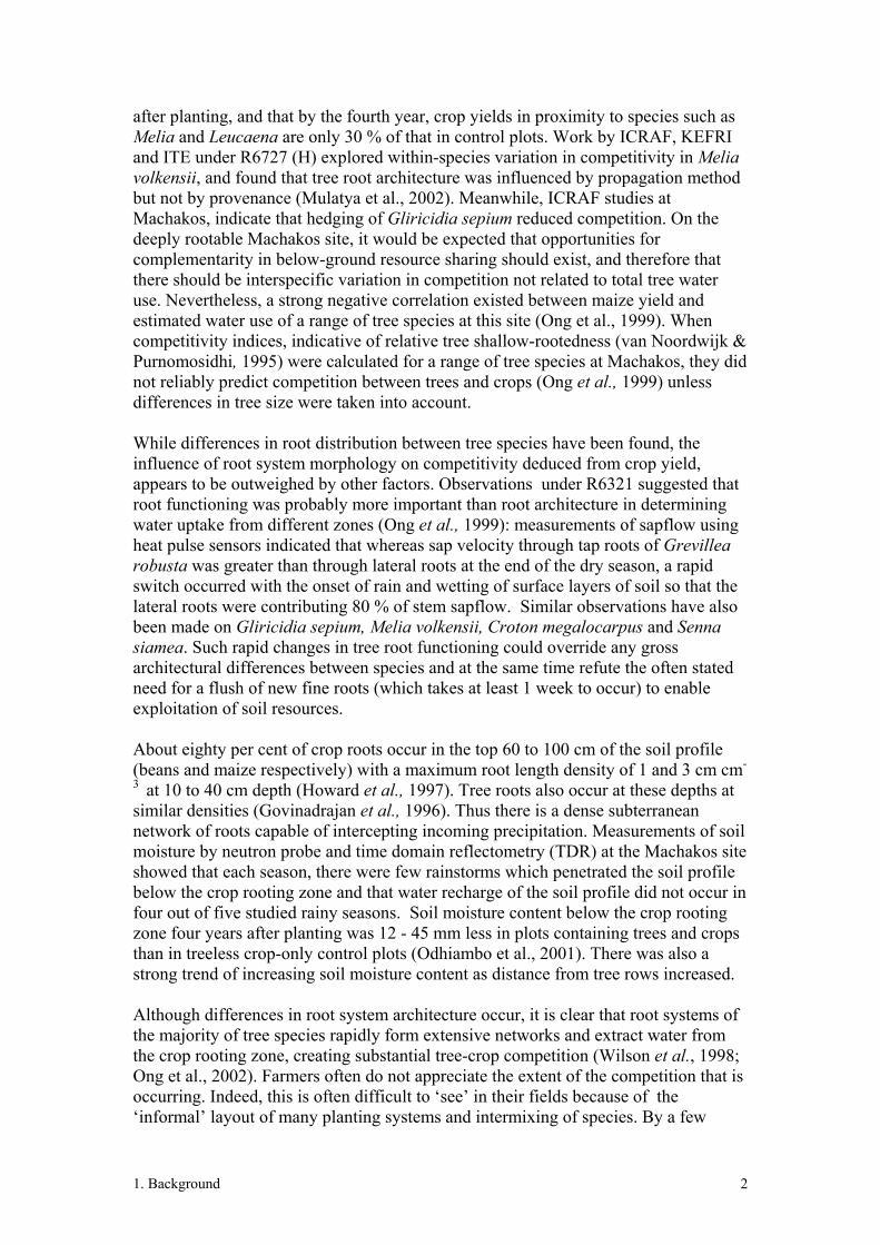
conducted at one site where sufficient trees were available. Timing of pruning was determined by local farmer practice - it was carried out towards the end of the dry season, to minimise potential disturbance to adjacent crops, and when there is labour available. Assessments were made at the sites listed in Table 3.1-1 (Okorio et al. 1994; Peden et al. 1997). At Kabanyolo, assessments focussed on amounts of biomass removed at pollarding and subsequent survival, while at the other sites, subsequent growth was also assessed. Table 3.1-1 Sites used for large tree pruning studies
Country Location Annual rainfall (mm) and temperature
Planting date
Design Tree species available for the study
Uganda Kabanyolo 1 University Farm, Mpigi. (0º 28´ N, 32º 27´ E, 1250 m.a.s.l.)
1400 mm bimodal mean min. 15.7º C max 27.9º C
1988 randomised complete block design, with crop only control, 3 blocks. Plots are 16 x 6 m, with a single row of trees planted 2 m apart along the long axis.
Alnus acuminata, Casuarina equisetifolia , Maesopsis eminii, Markhamia lutea, Melia azederach, Cupressus lusitanica, Cordia abyssinica
Uganda Bushenyi District Farm Institute, Bushenyi. (0º 34´ S, 30º 13´ E, 1610 m.a.s.l.)
1168 mm bimodal mean min. 13.5º C max 25.6º C
19907 5 – 15% slope Linear planting on contour rows, 3 replicate plots, 5 trees per plot
Acacia melanoxylon, Periserianthes falcataria, Alnus acuminata, Causarina cunninghamiana, Casuarina equisetifolia, Casuarina glauca, Eucalyptus grandis, Grevillea robusta, Maesopsis eminii, Polyscias fulva,Cupressus lusitanica, Cordia abyssinica
Uganda Kalengyere Highland Crops Research Station. (1º 15´ S, 29º 45´ E, 2470 m.a.s.l.)
1082 mm bimodal mean min. 11.9º C max 21.2º C
19901 10 – 25 % slope Linear planting on contour rows, 3 replicate plots, 5 trees per plot
Acacia melanoxylon, Periserianthes falcataria, Alnus acuminata, Causarina cunninghamiana, Casuarina glauca, Cedrela odorata, Eucalyptus grandis, Grevillea robusta, Polyscias fulva, Melia azederach, Markhamia lutea
Uganda Kachwekano District Farm Institute (1º 16´ S, 29º 57´ E, 2000 m.a.s.l.)
988 mm bimodal mean min. 10.4º C max 23.8º C
19901 25 – 45 % slope Linear planting on contour rows, 3 replicate plots, 5 trees per plot
Acacia melanoxylon, Periserianthes falcataria, Alnus acuminata, Causarina cunninghamiana, Casuarina glauca, Cedrela odorata, Eucalyptus grandis, Grevillea robusta, Polyscias fulva, Markhamia lutea, Maesopsis eminii
Kenya Siaya Institute of Technology Farm (00 04’N, 340 17’E, 1300 m.a.s.l.)
1200 mm bimodal
19958 Randomised design, 5 basal P treatments x 3 reps x 6 tree species. Plots are 7 m long, 4 trees per plot with a central tree row. Intercropped with sorghum. Plots have never been trenched.
Eucalyptus camaldulensis, Alnus acuminata, Cedrela serrata, Markhamia lutea, Casuarina equisetifolia, Grevillea robusta
7 In 1994, prior to this study, trees in Kalengyere, Bushenyi and Kachwekano trials were cut to the ground for assessment of biomass production and pole quality. 8 Crop assessments were also done at this site

3. Research activities 8
3.1.4 Output 4. Potential of early crown pruning of young trees as a means of controlling competition examined and quantified
While the work under output 3 above examined the effects of pruning large trees, we took over the support of an existing pruning trial at the Kifu site, in which trees have been subjected to different crown pruning treatments from a young age (Kifu 1 Table 3.1-2). Effects of pruning on tree growth and productivity and intercrop yields (mass) (cassava) were determined. Table 3.1-2 Other pruning study sites: early crown pruning at Kifu 1 and root pruning at Kifu 2 and Nyabeda. Country Location Annual
rainfall (mm) Planting date
Design Tree species available for the study
Uganda Kifu 1 Kifu Forest Research Station 0º48´N, 32º 46´ E, 1250 m a.s.l
1400 mm bimodal
1996 Randomized complete block design, 3 blocks, 3 different pruning intensities (removal of bottom 1/3, 2/3 of canopy and pollarding (whole crown removal), with control
Cordia africana, Grevillea robusta, Senna spectabilis
Uganda Kifu 2 Kifu Forest Research Station 0º48´N, 32º 46´ E, 1250 m a.s.l
1400 mm bimodal
1995 Randomised block design, with crop only control 25 trees per plot, 4 blocks with a central tree row. Trees currently at 1 m spacing, due to be thinned in 1999.
Alnus acuminata Grevillea robusta, Maesopsis emininii Casuarina equisetifolia, Markhamia lutea
Kenya Nyabeda School Farm
1800 mm bimodal
1993 Randomised block design, 2 basal P treatments, 1 tree species and crop only control, central tree row, 15 trees per plot.
Grevillea robusta,
3.1.5 Output 5. Potential of root pruning of trees as a means of controlling competition for water and controlling zones of water extraction examined and quantified.
Above ground pruning provides the opportunity to reduce transpirational demand, while below ground pruning would appear to enable manipulation of zones of water uptake so that tree water uptake from horizons exploited by crop plants could be reduced by pruning of surface lateral roots close to the tree's trunk. This would increase complementarity of resource sharing and reduce competition with crops. Our own recent data (R6321) (Ong et al., 1999) suggested that tree roots were capable of adjusting their activity in response to changing conditions, and that most water uptake during the dry season occured through the taproot while much of that during the rains was via the lateral roots. What is not known, is whether, if lateral roots are pruned, the tap root will be able to supply sufficient water to drive tree growth throughout the year and what the impacts of this redistribution of water uptake would be upon deep soil water content and recharge which studies at Machakos have already demonstrated are adversely affected by trees.

3. Research activities 9
Work under output 3 was directed at determining the feasibility of pruning large trees to reduce their competivity after competition has been well-established, work under this output was directed at evaluating the prospects for pruning young trees to regulate their competivity. This work was conducted on sites with trees of similar age, but with differing rainfall. Originally, it was planned to include ICRAF’s experimental farm at Machakos (Kenya) and their trial at Siaya2 as study sites. However, Machakos ceased to be available, and trees at Siaya2 were judged to be too small. Consequently studies were focussed at Kifu2, in Uganda, and Nyabeda (near Siaya). Tree and crop productivity under different pruning regimes were determined, alongside soil moisture and sapflow measurements where appropriate (Table 3.1-2).
3.1.6 Output 6: Potential of severe shoot and root pruning for controlling competition between trees and crops investigated in on-farm trials, with farmer evaluation of pruning effects, and methodologies, consequences and costs. Techniques and information disseminated through ‘farmer days’.
Farmers were directly involved from the start of the project through on-farm experimentation and farmer days at field sites. The main on-farm experimentation was conducted in the Katuna Valley (Kabale region) of Uganda, utilising a completed existing on-farm trial of Grevillea and Alnus. Tree and crop growth were measured and crown and combined crown and root pruning methods were evaluated.
3.1.7 Output 7: Dissemination of results of project by pruning bulletins, farmer days, contract reports, scientific papers and final workshop.
An additional, special item was subsequently added to this category, when representatives of the community in Kabale were taken on a mini-bus visit to farmers in Embu Kenya, to see pruning in action and be exposed to a diversity of farming activities. A video was produced in three languages. This activity was jointly funded by USAID.
3.2 Phase 2
3.2.1 Continuation of Outputs 3 & 5: Improved understanding of tree species’ tolerance (survival and regrowth) of combined crown and root pruning, and the impacts of pruning on tree growth – with extension of studies into drier zones.
This study involved a) continuation of ongoing work at Siaya1 b) new studies at Kitui and Kibwezi which are in drier locations, using some species which have already been studied in wetter zones and some new species and c) studies in Uganda in the Kigezi Highlands (Kabale) where we worked in the main project, and in Masaka District, which is a new area. We knew that the trees survived the treatments at Siaya, but the reason for continuing the studies there was to obtain better information concerning the impacts of pruning on tree growth rates (dbh), which were beginning to show signs of

3. Research activities 10
being affected. Studies at Kitui and Kibwezi would enable us to determine whether the drier climate affects tree species’ response and survival after pruning and also to test out further tree species to assess the ‘universality’ of the techniques, and will have close involvement with farmers. Studies at Masaka were dropped due to difficulties with a subcontractor and effort was redirected at Kabale. Involvement of local people at Kabale, Kibwezi and Kitui was increased through direct involvement of community groups.
3.2.2 Continuation of Output 6: Effects of combined root and crown pruning on crop yield assessed in drier zones
On-farm assessments of crop yield were continued at Kabale and new studies commenced at Kibwezi.
3.2.3 Continuation of Output 5: Improved understanding of root pruning effects on soil moisture profiles
Obtain additional soil water data to determine effects of root pruning on soil moisture profiles, infer impacts of tree root pruning on leaching effects and investigate aspects of root ‘redundancy’ through root regrowth and soil water observations. This will be done using a more widely spaced trial at Siaya 2 (planted 1997), using profile probes to obtain detailed information of water infiltration and recharge on root pruned and unpruned plots of Eucalyptus camaldulensis and Grevillea robusta, with and without crops, and with ‘no tree’ controls.
3.2.4 New Output 1: HyPAR model improved Parameterise HyPAR model and modify to simulate pruning. Once calibrated, analyse patterns of observed and modelled soil water depletion with unpruned trees and their relationship with crop growth. Apply fractal techniques to estimate tree fine root length regrowth and model the relationships with crop growth, utilising data collected previously. Explore how well root ‘redundancy’ and variable ‘uptake efficiency’ are covered in the model. Verify the calibrated model.
3.2.5 New Output 2: Simple economic model developed Identify the factors that can affect income, create the structure for the economic model by using project data. Collect economic unit value required to value all impacts on farmers’ income caused by the implementation of pruning techniques. Quantify the economic changes associated with pruning and assess on economic grounds the reasons for farmers to undertake (or not undertake) tree pruning.
3.2.6 New Output 3: A biophysical assessment of the situations in which pruning is likely to be effective and the socioeconomic circumstances in which it is likely to be adopted
Using data collected under 1, 4, 5 and 6 and taking into account global distributions of agroclimatic zones, farming patterns etc, produce an assessment of circumstances where pruning is likely to be effective and adoptable.

3. Research activities 11
3.2.7 New Output 4: Survey of farmer uptake of pruning regimes Farmer uptake of pruning regimes will be obtained by re-surveying sites active under the main project R7342, and monitoring farmer response to work ongoing under this project extension.
3.2.8 Continuation of Output 7: dissemination of results and promotion of pruning
In this report, presentation of results from Phase 1 and 2 will be combined where appropriate.

Results 4.1 – Summary of findings 12
4 Results and discussion
4.1 Summary of findings
4.1.1 Pre-project tree pruning practices in Kenya and Uganda
Pruning practices At the Kenyan sites, pruning was widely practiced, and a variety of pruning methods were used. At Siaya, farmers practiced side pruning, pollarding or both, mainly in order to
reduce competition with crops. 63 % had observed that crop growth was improved by pruning, and the majority of farmers gave root competition rather than shading as the reason for this. However only 5 % of farmers had cut roots to control them.
At Embu, all farmers used pruning, the majority combining side pruning and pollarding. All farmers observed a positive response by crops to pruning and recognised root competition as a problem. In this district there were more attempts at manage root competition and 39 % of farmers had cut roots or dug trenches. Pruning of timber species such as Grevillea, Eucalyptus, Melia and Markhamia was commonly practiced to reduce shading, improve stem quality and provide wood for household needs.
At Kibwezi was selected for comparison since tree pruning was more developed at this site. Farmers recognized that competition occurred between trees and crops, and that crop yield was reduced. 88 % of farmers pruned branches to manage competition, and 2 % pollarded.
At the Ugandan sites pruning was less widely practiced and developed. At Kabale in particular, pruning was less prevalent, although Eucalyptus was
commonly pruned in the early years of growth to give a straight bole. Trees were rarely pruned severely and most took ‘a fraction’ of the branches. Of those who pruned, 34 % also pruned Grevillea to produce a straight stem. The most usual reason given for not pruning was lack of labour, although tree-climbing dangers, lack of time and tools, crop damage and harmful insects were also cited.
At Mukono pruning was more prevalent, with 58 % of farmers pruning their trees in order to reduce competition and improve crop yield. Species pruned included Artocarpus, Ficus, and Maesopsis.
Farmer views of pre-project pruning practices Effects on crop yield:
• 90% of farmers in the Kenyan study sites (Siaya and Embu) observed positive changes on crops after crown pruning, however they still found fields with trees to perform less than those without. The majority recognized the problem as root interference with crops, although most did not take any measures to manage the problem because they did not know of any solutions. A few farmers used trenches to avoid tree roots spreading in to the crop fields.
• At Mukono half of respondents did not know whether pruning produced positive or negative effects on crop growth, although almost 40% reported that pruning conferred positive effects.

Results 4.1 – Summary of findings 13
Effects on trees:
• Almost all farmers observed that pollarding Grevillea, Markhamia, Melia and Eucalyptus species resulted in coppicing afterwards, and some observed faster growth after pollarding.
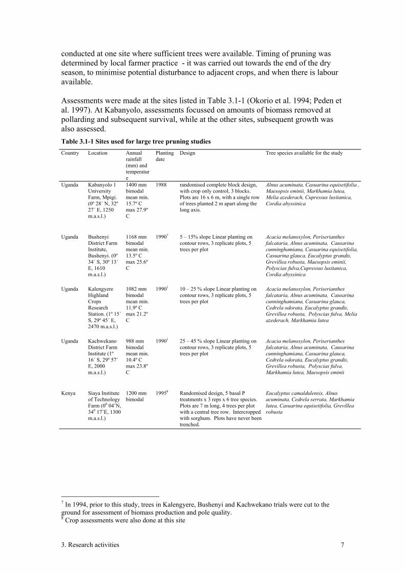
Other benefits of pruning In Siaya and Embu most farmers used tree prunings as firewood, and bigger
branches for building houses. More than a quarter of farmers with surplus prunings sold the wood and used the proceeds for household needs. Some farmers left tree branches on farm as mulch and manure.
At Kibwezi by contrast, where pruning is widely practiced, tree prunings are not sold, but used for fuelwood, poles, fodder or mulch.
At Kabale, the majority used prunings for firewood or stakes, although the shortage of firewood was not met with increased pruning because there was a belief that pruning some species would lead to tree death.
Comparison of farmers’ pre-project tree pruning practices All sites were similar in the timing of pruning: one annual prune falling at the end of the dry season before crop planting, or at the
beginning of the wet season when shade cast by the trees was becoming a limitation on crop growth.
Pruning at all sites was largely the responsibility of male household members, generally the male head of household or a male child.
A surprising finding of the study was the extent of the differences between sites, which covered almost all aspects of tree management. The Kenyan sites were in general more knowledgeable and experienced in their use of pruning to manage competition between crops and trees, and had more developed pruning methods including root pruning, used a wider variety of tools, and employed pruning materials more widely on-farm or to generate income. The Ugandan sites, Kabale in particular, were less knowledgeable and experienced in pruning techniques, although there was consistent practice of pruning to manage timber quality. Differences in tree management practices will arise for a number of reasons, including the extent to which knowledge about tree management has been passed down through the generations, training and dissemination activities at different locations, pressures on land, availability of off farm income, the likelihood of crop failure, and the uses to which trees are put. At Kabale in Uganda, over a quarter of farmers said that they had learned about trees in 1994, 96 and 98, which coincides with ICRAF/AFRENA activities in the area when extension organizations were training farmers on tree management on-farm. Most stated that they had learnt in childhood, or never learned. It was observed from the study that although some pruning was practiced, there seemed to be little understanding of reasons for pruning. By contrast, at Kibwezi where crown pruning was widely practiced and also some root pruning, 17 % of farmers had received specific training in crown pruning, and 10 % in root pruning.

Results 4.1 – Summary of findings 14
4.1.2 Impacts of pruning on tree growth and survival When ‘old and large’ trees > 9 years old were pollarded, substantial amounts of biomass were produced. At Kalengyere, Kachwekano and Bushenyi, where some trees had been coppiced 5 years previously, tree size and biomass yielded were reduced by about 50 % when trees had been previously coppiced. At two sites, (Kachewekano and Bushenyi) survival of some species after pollarding was considerably reduced when they had been previously coppiced. These trials had a chequered management history and the data need to be treated with a degree of caution, however it is clear that previous coppicing had considerable long-term effects on tree growth and when large trees were pruned, some species were more resilient than others. Survival rates will be influenced by site conditions and tree vigour, but data from these sites and Kabanyolo, suggest that although Acacia melanoxylon, Alnus acuminata, Casuarina spp. and Cupressus lusitanica showed reasonable vigour before pollarding, their survival may be affected by cutting and it should not be recommended that they are pruned for the first time at this age, under similar site conditions. Many conifers do not respond well to severe pruning and while Cupressus can be side pruned to produce a clear bole, it should probably not be pollarded. When ‘young and small’ trees, 4 – 6 years old were pollarded (at Siaya, Kifu 1, Kifu 2, Nyabeda, and on-farm at Kabale) no problems of tree survival were encountered with any of the species studied. Effects on dbh developed gradually and significant reductions of 10 – 25 % were observed 1 – 2.5 years after pollarding. With repeated pruning, considerable reductions in tree growth will occur. While root pruning was less damaging to tree growth, and is often effective at removing competition with crops, crown pruning yields valuable products against which the reduction in tree growth rate must be weighed. Data from Kabale suggest that large numbers of trees could be planted on farms to produce wood products and that they could be managed to minimise competition with crops, but longer term studies are needed to gain a better picture of survival and biomass production with repeated pollarding. Data from Kabanyolo and Siaya highlight the large numbers of epicormic shoots produced by some species after pollarding, which need to be reduced to preserve bole quality and yield useful stakes and poles. Although the first pollarding of large trees may take 20 – 30 minutes per tree and root pruning 10 or more minutes depending on method and soil conditions, repeat pruning is much quicker. Pollarding is best accomplished in the dry season when there are no crops to be damaged, and root pruning may be done when land is being prepared for crop sowing.
4.1.3 Impacts of pruning on crops Research station studies With densely planted trees at Siaya, the introduction of pruning enabled the successful production of intercrops, which had not previously been possible for some time. Generally, crown pruning alone, or in combination with root pruning, was more successful than root pruning alone. Root pruning alone was particularly ineffective for Casuarina. Results indicated that at this site, removal of the dense canopy was

Results 4.1 – Summary of findings 15
essential to reduce interception of rainfall. Pruning improved crop yields, especially during the two subsequent seasons, and often resulted in yields similar or greater than those on plots without trees. Crops growing with Eucalyptus were most responsive to pruning. The corresponding soil water studies showed that combined crown and root pruning improved soil water amounts relative to the other pruning treatments, but did not eliminate the effects of trees on soil water. At Kifu1, where different intensities of crown pruning were tested, maize was most responsive to canopy reduction and cassava was the least. When root pruning on one side of tree rows was tested at Kifu2. The yield of crops on the pruned side was considerably increased, but was counteracted by a corresponding reduction in yield on the unpruned side, presumably due to a compensatory increase in root activity on that side. Grevillea was the least competitive species. While these results clearly indicate that one-sided root pruning should only be used in limited circumstances (e.g. trees on roadsides and adjacent to compounds), results from Nyabeda1 indicated that compensatory root activity did not always occur. Results from Nyabeda 2 showed that increased soil water in the surface layers resulting from restriction of tree root activity by root pruning, was quickly utilised by crops, so that effects of root pruning on soil water were only apparent when land was not cropped. From the point of view of optimising crop yields, repruning of crowns and roots should probably be repeated annually, however if farmers wish to use poles or other tree products resulting from pruning, then annual crown pruning would be too frequent. However, rates of root regrowth were such that repeat root pruning annually would be advisable. On-farm studies Two studies were conducted at two sites which were very contrasting climatically, and pruning was effective at both. At Kabale, with 1200 mm rain annually, bean yields in the first season after pruning Alnus acuminata and Grevillea robusta were doubled by pollarding in the 5 m closest to the tree row, and were more than trebled by combined pollarding and root pruning. Tree pruning often resulted in yields which were similar to those on plots without trees. Alnus was the more competitive tree species. Effects diminished as tree regrowth occurred and if maintaining crop yield is the priority, then pruning should probably be repeated annually, while if tree products are more valued, then a wider time interval between pruning would be preferable. Pollarding and root pruning were also successful at reducing competition with Melia volkensii at Kibwezi (500 mm rain annually, bimodal). Combined pollarding and root pruning was the most successful treatment, but treatments applied separately were also effective. Studies at this site were too short term to determine the required frequency of root pruning.
4.1.4 HyPAR modelling Introducing pruning into the model was a challenge, which was not fully accomplished. Pollarding, with removal of part of the trunk cannot be correctly modelled because of inbuilt relationships between trunk diameter and tree height,

Results 4.1 – Summary of findings 16
which proved too complex to alter within the time available in this project, but crown pruning, of up to 90 % of the crown removed from the base up, could be modelled. Similarly, root pruning was difficult to implement dynamically because of inbuilt ratios between foliage and root biomass. However, in disaggregated mode where the tree parameter set has extra values controlling root distribution, it was possible to mimic regular root pruning by setting one of these parameters to a smaller value. Patterns of tree and crop growth were examined with pruned and unpruned trees over a 15 years simulation period, and data were input into the economic model.
4.1.5 Economic modelling The economic modelling highlighted the importance of diversifying farmers’ income through agroforestry, and the need to control tree growth by pruning to enable subsistence farmers to strike a balance between meeting their short and long term needs. Agroforestry systems provide security to farmers especially during times of erratic crop yield and unstable prices. However the profitability of agroforestry systems is very dependent on tree prices and encouragement to plant a diversity of high value trees is important.

Results 4.2 – Pre-project survey of pruning practices 17
4.2 Survey of farmers’ tree pruning practices in Kenya and Uganda (Survey protocol no.1 – see Annex 1)
4.2.1 Objectives • To make a survey of common tree pruning practices on-farms, • To evaluate these practices in the light of local experiences (advantages,
disadvantages and constraints), • To identify similarities and differences in farmers tree pruning practices • To determine why the different areas differ in tree management practices
4.2.2 Background information
Kenya
Embu Embu District is located in Eastern province on the Southeast slope of Mount Kenya with total land area of 2714 square kilometres. The coffee based land use system covers about 15% of the land and harbour about 60% of the population of Embu (Thijssen et al., 1993). Altitude ranges from 1280 to 1340 metres above sea level. The rainfall is bimodal and averages between 950 to 1200 mm per year. The soil is deep Nitisol of medium fertility. Embu has an average farm size of 1.3 hectares and a population density of about 500 person/km2.
Siaya Siaya District is located in Nyanza province of Kenya and is predominantly a crop based land use system. The district has an area of 3,528 square kilometres of which 1,005 square kilometres are under Lakes Sare and Kanyboli, adjoining the Yala swamp, and portion of Lake Victoria (Siaya District Development Plan, 1984/1988). Siaya has an altitude of about 1300 metres above sea level and an average rainfall of about 1200 mm per year. Soils are deep Oxisols. Siaya has an average farm size of 1.4 hectares and a population density of about 400 person/km2. Trees in both districts are found on farm boundaries, home compounds, scattered in crop areas and there are some woodlots.
Kibwezi Kibwezi is a division located in the Makueni District of the Eastern Province of Kenya, south east of Nairobi. It covers an area of 1251 square kilometres and was settled during the 1970’s, and thus has abundant areas still under bushed woodland and thicket bushland. The agricultural land use is predominantly subsistence farming. Rainfall is bimodal and averages 500-600mm per year. The area lies on eroded flood plains, ranging from calcareous and non-saline to extremely calcareous and saline. Kibwezi has a population density of about 30 person/km2.
Uganda
Central Uganda

Results 4.2 – Pre-project survey of pruning practices 18
In central Uganda, two districts were chosen for this survey, namely Mukono and Mpigi district. Both districts are approximately 1200 m above sea level, border Lake Victoria, and receive above 1000 mm of bimodal rainfall annually. The long rains start in February and end in June, while the short rains stretch from September to December. The soils are largely oxisols. The landuse system in the districts is based on coffee and bananas, mixed with a range of other crops. The population density is about 120 person/km2.
Kabale Kabale district has a temperate climate characterized by mean minimum and maximum temperatures of 100 and 230 C respectively. As in central Uganda, the rainfall distribution is also bimodal totalling 1000 mm and above annually. Although the area is mountainous, the favourable climate and the inherently fertile soils coupled with historical factors led to high population densities in the area (about 246 person/km2).
4.2.3 Methodology A survey (using structured questionnaire, see Survey Protocol no. 1) was used with specific objectives of assessing farmers’ tree pruning practices and their observations of tree-crop interactions on-farms. In Kenya, farmers at Siaya and Embu were visited randomly in the months of November, December 1998 and in September 1999. Farmers at Kibwezi were visited early in 2002, during the second phase of the contract. In Uganda the surveys were done in late 1999 and early 2000. Each farm visit and interview lasted between 30-45 minutes. The number of respondents and some of their characteristics in each survey are given in Table 4.2-1.
Table 4.2-1Characteristics of respondents at the different survey sites in Kenya and Uganda
Uganda Kenya Kabale Mukono Siaya Embu Kibwezi
No. respondents 82 54 19 15 42 % male 62 48 - - 53
% female 38 52 - - 47 Age class (%)
20 - 40 34 52 37 40 - 41 - 60 35 33 37 47 -
> 61 25 15 26 13 - Family size 5-8 children
(56 %) 6-10
children (59 %)
- -
Educational attainment (%) No education 16 7 - - - Primary only 46 52 - - -
Secondary 18 32 - - - Higher 20 9 - - -
Land ownership (%) owner 88 69 95 100 -
Tenant 10 28 5 0 - Squatter 1 2 0 0 -
% dependent on on-farm income
75 54 89 - 76
Income from off-farm activities
46 24
- not determined

Results 4.2 – Pre-project survey of pruning practices 19
4.2.4 Results
Socio-economic background
Land holdings In Kabale, where farming is conducted on scattered terrace plots, land holdings were expressed in terms of numbers of plots. 30 % of farmers owned between 1 and 5 plots, while 6 – 10 and 11 – 15 plots were each owned by 23 %. 13% owned 16 – 20 plots and 12% owned between 21 and 60 plots. At Mukono, 41 % of farmers farmed 2-3 acres. Between 1 and 22 of the plots held contained trees, but the majority of farmers (85%) owned between 1 and 4 plots with trees. In Siaya, 58 % farmed between 1 and 3 acres, while at Embu, land holdings were bigger and 80 % of farmers had 1.5 – 6 acres.
Fuel In Kabale, 93 % of farmers used firewood as their primary fuel. Charcoal was the predominant fuel of second choice. Paraffin, crop residues, dung and electricity were of decreasing and lesser importance. One respondent ranked electricity as their primary fuel source. In Mukono, 91 % of farmers ranked firewood first. Charcoal was the second choice, and paraffin was third. 85.2% did not use electricity and just 2 respondents ranked electricity as their primary fuel source. 41 % of Mukono farmers said that they produced their own fuel on their farm, while only 4 % said that they obtained it from the forest reserve. This is a rather low figure, considering that the sub counties selected from Mukono district border the Mabira Forest Reserve.
Tree planting on farms Trees were important to farmers at all locations (Table 4.2-2). Almost all farmers were able to identify niches available for tree planting and to plant trees. The range and number of tree species varied considerably according to location and uses of the tree products. A description of the most commonly planted tree species, their uses and management is given on page 32.

Results 4.2 – Pre-project survey of pruning practices 20
Table 4.2-2 Tree planting on farms at locations in the first survey
Uganda
Kenya
Kabale Mukono Siaya Embu Kibwezi % farmers planting trees
96 98 95 100 100
No. tree species reported
18 24 - - 54
Mean no. tree species per farm
5 6 44 % planted around homesteads and 22 % on fallow lands
- 47 % of farmers only planted within the homestead, 5 % on internal and external boundaries and the remainder planted in all locations.
- 26 % of farmers only planted in the homestead, 14 % on internal and external boundaries and the remainder planted at all locations.
- Home compound, 2 ‘natural’ species, 4 planted species. Grazing land: 2.5 species occur naturally, none are planted. Crop land 2.7 species occur naturally and 2.2 were planted.
Main tree species, and % of farms with species present (% planted by farmers if known)
Eucalyptus grandis 88 % (84 %) Grevillea robusta 46 % (45 % ) Cupressus 46 % (46 %) Avocado 38 % (38 %) Alnus acuminata. 38 % (38 %) Cedrela sp. 38 % (37 % ) Calliandra calothyrsus 34 % (34 %) Acacia mearnsii 32 % (20 %) Markhamia sp. 28 % (17 %) Erythrina sp. 24 % (18 %) Carica papaya 17 % (15 % ) Sesbania sp. 15% (12 % )
Artocarpus heterophyllus 81 % Ficus sp. 77 % Mangifera indica 77 % Avocado 68 % Markhamia 67 % Coffee 27 % Carica papaya 24 % Milicia excelsa 20 % Maesopsis eminii 20 % Sapium 14 % Psidium guajava 13 % Callistemon 7 %
Predominant timber species was Markhamia lutea, which was the only species planted with crops by 74 % of farmers.
80 % of farmers said they only planted Grevillea robusta with crops
In home compounds, 21 % of farmers had no natural trees. Stercula africana occurred naturally in 26 % of cases. All farmers had plamted trees including - Senna siamea (83 % ) & Carica papaya (36 %) In grazing land few trees were planted - Eucalyptus camaldulensis (2 % ); all farms had some natural trees, Adansonia digitata and Acacia tortilis in 7 % of cases. In cropland, Adansonia digitata occurred naturally in 48 % of cases and Melia volkensii in 17 % of cases 7 % of farmers had no natural trees, 24 % of farms had no planted trees. Carica papaya (40 %) Annona squamosa (24%) Psidium guajava (24 %) Mangifera indica (19 %)
The number of tree species occurring in farms, either naturally or planted.
Tree Planting in Central Uganda In Kabale, 50 % of the farmers interviewed did not plant trees, arguing that they did not have enough land or faced difficulties in acquiring planting materials. They however expressed strong interests in tree planting. Asked which species they would want to plant, 23% preferred planting black wattle for charcoal and 50% wanted Calliandra calothyrsus for fodder, contour hedges, tree seed production for sale, stakes for climbing beans and firewood. Few species were viewed by farmers as income generating. Only 18 % said they would plant pines, while 50 % favoured Cupressus lusitanica because of its live fencing qualities. Markhamia lutea was

Results 4.2 – Pre-project survey of pruning practices 21
another desirable species because of its coppicing ability. It is used locally for firewood, climbing stakes and poles for local construction of temporary houses. Of those who plant trees at Kabale, 56 % planted trees in their agricultural fields. When planting along boundaries, 29 % of farmers discussed it with their neighbours, and 13 % gained the agreement of their neighbours. At Mukono, 52 % of farmers planted trees in their agricultural fields. When planting along boundaries only 15 % discussed it with their neighbours and only 6 % had an agreement with their neighbours. Most of the farmers interviewed reported that opportunities existed for them to plant trees on their plots, mainly around homesteads (44.4%) and fallow land (22.2%). Only a very small proportion (2%) indicated that they did not have opportunities to plant trees on their farms. Husbands and wives planted almost an equal number of trees on the farms. For those farmers that planted trees along the boundaries, the majority (approximately 65%) did not discuss with their neighbours before planting trees on the boundaries. A small proportion (15%) discussed with their neighbours before planting trees along boundaries. At Kabale, those who plant Eucalyptus are considered rich farmers who have extra plots of land for establishing separate woodlots. Generally, Acacia mearnsii (Black wattle) and pines are never planted with crops for fear of severe competition. 60 % of the respondents observed that Eucalyptus competed highly with crops for water while Markhamia, Calliandra, Coffee and Erythrina were rated as the least competitive. Alnus and Grevillea were reported to compete moderately for water and light yet farmers still want them because of their very useful products. For Alnus (40 %), Grevillea (40%) and Calliandra (20 %), the main planting niche is in compounds. The responses given by farmers in Kabale on how they benefit from the trees on their farms are summarized in Table 4.2-3, below. Table 4.2-3 Kabale farmers' views on benefits of tree species (% of respondents).
Species
Timber
Fuelwood
Cash
Not applicable
Others
Alnus acuminata 40 7.5 5 35 12.5 Acacia mearnsii 27.5 67.5 5 Calliandra calothyrsus 2.5 2.5 50 45 Cedrela serrata 37.5 5 45 12.5 Cupressuss lusitanica 22.5 2.5 2.5 50 22.5 Erythrina abyssinica 70 30 Eucalyptus grandis 17.5 45 32.5 2.5 2.5 Grevillea robusta 50 10 2.5 25 35 Markhamia lutea 7.5 22.5 57.5 12.5 Pinus patula 12.5 82.5 5 The “Others” column in the table above includes such uses as soil conservation, compost/mulch, fodder, stakes for climbing beans, shade, amenity, fruits and fences. No specific tree species is grown for a single purpose. No farmer mentioned any of the above species as a medicinal tree, however most local people who use medicinal herbs do not like to give “strangers” this information, in order to protect their source of income. Timber production is clearly a priority use for Grevillea robusta and Alnus acuminata. Interestingly, Kabale farmers have not generally practiced timber production, so this demonstrates that they are aware that it is a good income-

Results 4.2 – Pre-project survey of pruning practices 22
generating commodity. This awareness would suggest an understanding of the need to manage them for timber quality.
Tree Planting in Kenya At Siaya, the tree most commonly planted with crops was Markhamia, and 63 % of farmers noted that crops grew less well close to the trees. At Embu, Grevillea was the commonest tree with crops and 80 % of farmers reported heavy competition adjacent to crops. Embu farmers mix mainly maize and beans with trees while farmers in Siaya mix mainly maize. Farmers in Kenya were questioned about recognition of niches for trees on farms: these were identified as homestead9 (91.2%), hedgerow in cropland (29.4%), internal and external boundaries (8.9%) (Table 4.2-4). Farmers who planted trees along agricultural fields observed shading effects on crops regardless of species. Tree planting in Embu and Siaya varied slightly in planting arrangements; Embu district planted trees mainly in line arrangement while Siaya district planted in both scattered and line arrangement. Table 4.2-4 Niches for trees and tree planting arrangements used by respondents in Kenya
Embu and Siaya Kibwezi Niches n % respondents n % respondents
Homestead 31 91.2 - Hedgerow in crop land 10 29.4 -
Internal and external boundaries 20 58.9 36 Total10 61 179.5 -
Arrangements
Line 14 41.7 3 7 Scattered 7 18.4 34 81
Line and scattered 9 28.6 - Other arrangements 2 5.7 3 6
Bench terrace - - 6 14 No response 2 5.6 0 0
- not asked
When questioned about the purposes of tree plantings on farms, farmers in both Embu and Siaya districts grow trees mainly for fuelwood, construction poles, timber, shade, windbreak, boundary demarcation, fencing, fruits, beautification, cash generation, and medicine. Farmers in Embu used tree wood for tobacco curing. Few farmers in Embu reported the use of Grevillea leaves for roofing. The most important and widely grown species in Embu and Siaya are Grevillea robusta and Markhamia lutea respectively. Melia volkensii is common in the lower Embu. In the Kenyan districts, when asked about constraints in growing trees, farmers cited pests, shortage of labour during peak seasons, competition of trees with crops, lack of tree seeds and seedlings as some of the major constraints in Embu and Siaya districts.
9 Around homes 10 n and % came to more than 34 and 100 respectively as farmers used more than one niche for planting.

Results 4.2 – Pre-project survey of pruning practices 23
Knowledge of competition Farmers at Kabale described their trees as competitive more frequently than those at Mukono (Table 4.2-5). 44 % of farmers considered that competition was mainly for water and 20 % considered it to be for light. The most competitive tree was stated as Eucalyptus, followed by Acacia mearnsii, Alnus, Grevillea and Cupressus. 51 % of farmers at Kabale said that crop yield next to trees was a lot less than in the rest of the plot. The species composition is rather different at Mukono, here, the maximum amount of competition (43%) was reported for Sapium, which was rarely planted. Maesopsis and Artocarpus were the next most competitive, followed by mango and Markhamia. Surveys at Siaya and Embu did not assess competition by individual species, but 68 % of farmers at Siaya considered heavy shading by trees to be a problem, and 16 % commented on light shading. At Embu, 80 % of farmers reported heavy shading and only 7 % reported no shading. At Kibwezi, the 2 species most commonly grown on cropland by farmers were Adansonia and Melia, the majority of farmers described both of these trees as competitive. None of the other species were present in sufficient number to firmly allocate competitiveness, but approximately 50 % of farmers considered most of the species to be competitive. Table 4.2-5 Farmers' perceptions of competition by different tree species
% of all farmers who described a species as competitive
Shades crops Competes with crops
% of farmers who planted the species
Propn of growers who found it competitive
Kabale Eucalyptus 12 42 88 61 Grevillea 6 11 46 37 Alnus 8 8 38 42 Erythrina 1 4 24 21 Cedrela 2 4 38 16 Cupressus 4 9 46 33 Calliandra 1 2 34 8 Acacia mearnsii 1 15 32 50 Markhamia 1 1 28 7 Sesbania 1 0 15 7 Avocado 4 2 38 16 Carica papaya 1 0 17 6 Mukono Artocarpus 11 9 81 25 Ficus 9 2 77 14 Mango 11 4 77 19 Avocado 6 2 68 12 Markhamia 2 10 67 18 Coffee 0 0 27 0 Carica papaya 0 0 24 0 Milicia 2 0 20 10 Maesopsis 6 0 20 30 Sapium 2 4 14 43 Guava 0 0 13 0 Calliandra 0 0 7 0 Kibwezi Crop land Adansonia digitata 74 90 0 90 Melia volkensii 45 100 10 100

Results 4.2 – Pre-project survey of pruning practices 24
Tree management
Prevalence of pruning and pruning strategies At Kabale, 72 % pruned their Eucalyptus trees, and 42 % of farmers started pruning within the first two years, and only 6 % pruned trees when they were older, with the stated objective of reducing competition. The usual reason for this early pruning was to give a straight bole. Trees were rarely pruned severely; this was only reported by 5 % of farmers for Eucalyptus and for no other species, and most took ‘a fraction’ of the branches. Of those who pruned, 34 % pruned Grevillea, 11 % of those pruning to produce a straight stem. Only 7 % of farmers thought that Grevillea competed with crops for water, and 15 % thought it was for light. Cupressus was always pruned, usually to give a straight stem. Pruning was not as prevalent at this site compared with Mukono or the Kenyan sites. The most usual reason given for not pruning was lack of labour, although when questioned about this specifically, reasons cited as the major problem were the risks involved in climbing trees. Other problems listed included lack of pruning tools, the fear of damage to crops by falling branches, fear of harmful insects in the foliage, while others indicated that pruning is time consuming. When questioned about the extent of shoot pruning of specific species, the responses were as shown in Table 4.2-6. Table 4.2-6 Pruning of commonly grown tree species by Kabale farmers.
Species Pruned Not pruned Not applicable Alnus acuminata 65.5 7.5 27.5 Cupressuss lucitanica 42.5 2.5 55 Eucalyptus grandis 70 22.5 7.5 Grevillea robusta 62.5 12.5 25 Markhamia lutea 12.5 22.5 65 Pinus patula 7.5 5 87.5
At Mukono 58 % of farmers pruned their trees and 28 % pruned or cut trees down to reduce competition. Farmers had a different approach to pruning, compared with Kabale. At Mukono, there was no emphasis on early pruning, and 39 % of farmers said they started pruning when there were large branches on the tree. 22 % of farmers pruned Artocarpus, mostly (17 %) by removing a fraction of the branches. Although farmers had not rated Ficus as being particularly competitive, 30 % of farmers pruned it and about half these farmers pruned it severely. A few farmers pruned Maesopsis with the objective of producing a clean bole. 21 % of farmers considered that pruning improved crop yield. Interestingly, 48 % of farmers considered that they had problems with tree roots on farms. 18 % avoided planting crops in these areas, while 35 % root pruned or removed trees. 6 % considered that the tree products were more valuable and the same proportion said they could do nothing because the trees were not under their control. At Siaya where Markhamia was the most commonly planted tree with crops, 47 % of farmers side pruned and 36 % pollarded or did both, but only 15 % did this to reduce

Results 4.2 – Pre-project survey of pruning practices 25
competition. 63 % had observed that crop growth was improved by pruning. 63 % also said that they had observed root competition, only 5 % of farmers had cut roots to control them, the remainder did nothing. At Embu, all farmers used pruning on Grevillea, and 67 % combined side pruning and pollarding (Plate 1). All farmers observed a positive response by crops to pruning. 67 % of farmers had observed root competition. There were more attempts at this site to manage root competition and 39 % of farmers had cut roots or dug trenches. Most farmers at the Kenyan sites pruned pole/timber species such as Grevillea, Eucalyptus, Melia and Markhmia trees to reduce shading problems, to improve stem quality and get wood for household needs (Table 4.2-7). The most common types of prunings observed in both districts are side (branch) pruning and pollarding. Side pruning is practiced when farmers need the trees to grow faster and straight. The Embu farmers cut the canopy of Grevillea and Melia, at certain height, for diameter increment. Farmers in Siaya cut Markhamia at the base of the trees for coppicing. Most farmers in both districts do not prune fruit trees and trees planted as fences. They claimed that pruning fruit trees will reduce production, however, lower branches are removed for easy accesses. Some farmers did not completely remove the branches from the tree stem. They said this will ease next climbing for more pruning to take place. They also mentioned it helps trees to sprout faster.
Table 4.2-7 Summary of farmers' tree management activities at Embu and Siaya
Category n % respondents Degree of shading effects: Heavy shading Moderate shading Light shading No shading Could not tell Total
25 1 4 1 3 34
74 3 11 3 9 100
Reasons for pruning: Reduce shading on crops Get firewood & construction materials Improve wood quality and growth increment All (shade, fire wood, construction poles and improve wood quality) Total Types of pruning: Side pruning Pollarding Both side pruning and pollarding No pruning Total Reasons for not pruning: Get more fruit production Shade for human and animals Protection against wind and encroachment No time and labor to prune No response Total
4 2 3 25 34 12 7 12 3 34 16 1 2 4 11 34
11.8 5.9 8.8 73.5 100 35.3 20.6 35.3 8.8 100 47.0 2.9 5.9 11.8 32.4 100
At Kibwezi, many farmers recognized that competition occurred and that crop yield was reduced. 88 % of farmers pruned branches to manage competition, and 2 % pollarded. At this site, the most frequent reason given for pruning was to reduce competition. 59 % of farmers pruned between 25 and 50 % of the crown. 43 % of

Results 4.2 – Pre-project survey of pruning practices 26
farmers were aware of root competition, 10 % of farmers removed trees and the remainder took no action.
Knowledge about tree management At Kabale, 27 % of farmers said that they had learned about trees in 1994, 96 and 98, which coincides with AFRENA activities in the area, when extension organizations were training farmers on tree management on-farm. Of the remainder, 47 % said that they had learned when they were young and 5 % said that they had never learned. At this site in particular, pruning was a relatively new practice, and even where carried out farmers were unsure whether they were pruning for good timber or to control competition. When questioned, few Kabale farmers expressed a clear understanding of the relationship between timber quality and shoot pruning. A small number of farmers stated that they prune to reduce shading of other crops. Although farmers stated that pruning is a new practice at Kabale, these who pruned were not sure of the reasons why they practiced pruning. At Mukono, 46 % of farmers said that they had never been taught anything about trees, while 37 % learnt as a child. By contrast, at Kibwezi where tree pruning and even root pruning were widely practiced, 17 % of farmers had received training in crown pruning, and 10 % in root pruning. In Kabale, no farmer was found to be practicing root pruning at all. All of them thought it was not possible because the tree would die. Asked what they do when they observe problems caused by tree roots on farm, the following were the responses (Table 4.2-8): Table 4.2-8 Responses of farmers to root competition problems in Kabale.
Response % Dig root trenches (root prune) 0 Do not sow close to trees 71.4 Nothing, tree products are more valuable 19.1 No problem observed 9.5
Most farmers (71.4%) would abandon their fields if they observed that trees were competing with crops. Some farmers considered that specific tree species were known as “agroforestry trees” which they perceive as “miracle trees” that are compatible with their crops, and therefore assume that their tree species observed to compete with crops were not “agroforestry trees”. Tree species that farmers rejected for planting with crops included Eucalyptus grandis and Acacia mearnsii (Black wattle). Farmers at Kabale also had varying views on how a particular species competed for resources with crops on their farms (Table 4.2-9).

Results 4.2 – Pre-project survey of pruning practices 27
Table 4.2-9 Kabale farmers' views on competition between crops and tree species.
Species (% of respondents) Competition
Alnus Markhamia Acacia mearnsii
Calliandra Pinus Coffee Cupressus Erythrina Eucalyptus Grevillea
For water 12.5 0 20.0 0 7.5 0 20.0 0 60 15 For light 27.5 0 2.5 12.5 0 0 0 5.0 17.5 22.5
For space 5.0 2.5 0 7.5 0 0 2.5 0 2.5 5 Not aware 20.0 17.5 7.5 10.0 0 2.5 10 10 10.5 20
Not applicable
35.0 80 70.0 70.0 92.5 97.5 67.5 85.0 10.0 37.5
Sixty percent of the farmers reported that Eucalyptus competes highly with crops for water, while Markhamia lutea, Calliandra calothyrsus, Coffee arabica and Erythrina abssynica, were considered non-competitive for water. It is also interesting to observe that Alnus acuminata and Grevillea robusta are reported to be competing for all resources. These are relatively new species in this region and are highly demanded by the local farmers for agroforestry planting because they have been observed to grow very fast with a high potential for pole, timber and firewood production. Alnus acuminata in particular has been ranked as the highest quality firewood species (ICRAF Annual Report, 1995) and so far, the fastest growing species in the Kigezi highlands.
Who prunes? Although women provided most of the labour for farm activities, they play a minor role in tree pruning at all sites (Table 4.2-10). In the Kenyan districts, respondents who said women don’t prune trees gave various reasons. Sixty-eight percent respondents did not know why women are not allowed to prune trees while 20.6% respondents said it is just a tradition. Nine- percent of respondents considered pruning to be a difficult job for women. 3 % of respondents mentioned lack of ownership of trees. They said trees are for men and only men have the right to do what ever they want do with their trees, including tree management. The majority of respondents in Uganda (59.3%) reported that women do not prune trees, the reasons being that women are traditionally not allowed, they are weak and men and children can do it better. With the exception of Siaya, male children played a much stronger part, and at Kabale and Mukono, they did as much pruning as their fathers. Farmers at Siaya and Kabale employed most hired labour. Table 4.2-10 Distribution of pruning labour in farmer households (%)
Uganda Kenya Kabale Mukono Siaya Embu Kibwezi husband 29 42 53 50 55 wife1 5 14 15 11 0 male children 27 40 12 31 37 hired labour 39 4 20 7 8 1 women tended to only prune trees when they were young, unless there was a shortage of male labour
Tools for pruning At all sites, the majority of farmers used pangas for cutting branches (Table 4.2-11). Methods for access varied: farmers at Siaya had an overwhelming preference for using ladders, while at Mukono, farmers preferred to climb their trees. At Kibwezi,

Results 4.2 – Pre-project survey of pruning practices 28
the use of ladders would be impossible and climbing difficult for the very large specimens of Adansonia which are a feature of the landscape. In this situation, pegs are fixed into the trunk and used to provide hand and footholds. Table 4.2-11 Methods used for pruning and access of trees (% of respondents)
Uganda
Kenya
Kabale Mukono Siaya Embu Kibwezi For cutting panga 98 97 84 93 38 saw 2 3 10 0 0 panga and saw 0 0 5 7 0 For accessing high branches
ladders 53 20 89 80 38 tree climbing 26 38 0 131 41 no climbing 21 42 10 7 10 fixed pegs 122
1 ropes are used 2 Adansonia digitata
Timing of pruning, age of tree and costs of pruning At all sites, the majority of farmers pruned once a year, just before the planting season. In Kenya, farmers said trees will have time to utilize the coming rain for growing faster, avoid tree-shading effects on planted crops and damage caused during pruning. Pruning before the rain was also preferred, as farmers will be busy planting during the rain. Some farmers also indicated the importance of drying firewood in the sun and justified the need to do the prunings during the dry seasons. At Kabale, most farmers pruned during the rains, while at Mukono, the majority of farmers pruned Artocarpus and Ficus when they were causing shade rather than at a particular season. In Kenya, farmers start pruning when trees are young (2-3 years) and continue doing so, depending on species, size and age of the trees. Less commercially valuable species are not pruned as frequently as commercially valuable species. Fruit trees were also not usually pruned. The time spent in branch or crown pruning varied from respondents to respondents (Table 4.2-12). Fifteen- percent respondents said that they would prune their trees every 6 months (every season), while most (59%) said every year. Twenty-one percent said it depends on the species, size and age. Few (5.9%) said they would prune every 2 years or more. In Kenya the average cost of pruning was reported to be 29 KSh per tree, although could vary between 10 – 70 KSh depending on the amount of hired labour, size of tree and difficulty of pruning. Table 4.2-12 Time taken to prune a tree at Siaya and Embu
Category
n
% respondents
Less than 30mins 17 50 30-60mins 5 14.7 Depends on species, age and size of trees 6 17.6 Don’t remember 6 17.6 Total 34 100

Results 4.2 – Pre-project survey of pruning practices 29
At Kibwezi where there was a history of tree pruning, 71 % of the respondents did not hire labour for pruning. Only a minority (19%) hired labour. The cost of pruning a tree varies from farm to farm and also depends on the size of tree. On average, 75% of the farms pay KSh 50 per tree, while 13 % pay KSh.40 and another 13 % of the farmers pay KSh 20. 91% of the farmers indicated that only one person is required to prune a tree while the other 9% didn’t know because they have never pruned. Respondents indicated that this activity of pruning mainly takes places during the dry season so that falling branches do not damage crops. This is in the months of August, September and October. It is also the period when farmers have very little activity and therefore can afford to spend their time pruning. This therefore means that pruning does not in any way interfere with the schedule of other farm activities and should therefore be highly promoted.
Farmers’observations of the effects of pruning Ninety- percent farmers in the Kenyan study observed positive changes on crops after crown pruning, however they still found crops with trees to perform less well, compared to the crops without trees and most farmers suspect (76%) the problem as root interference with crops. Although farmers observed tree root competition with crops, most (68.2%) of them did not take any measures to manage the problem, because they did not know what to do with such problems. They think root management needs more time, money and labour. Very few (4.5%) farmers used trenches to avoid tree roots spreading into the crop fields. Some (27%) of farmers believed they may disturb tree roots unknowingly while preparing the land for planting crops. Farmers at Embu observed tree-shading effects on crops by comparing crop yield close to the trees and away from the trees. Seventy-one percent of respondents observed that crop production close to trees was very low compared to crops far away from the trees while 20.6% said production is the same. Eight percent of respondents did not see any difference. Almost all (97.1%) farmers in both districts observed that pollarding Grevillea, Markhamia, Melia and Eucalyptus species resulted in coppicing afterwards. Some respondents (6 %) observed faster growth increment in diameter, and 21 % said pollarded trees had both coppiced and grown faster. The majority of respondents at Mukono (50%) had no idea whether pruning produced positive or negative effects, while 38.9% reported that pruning conferred positive effects; 9.3% thought that pruning had negative effects.
Observed changes on soils under trees Most farmers in Embu observed poor soil fertility under trees while most farmers in Siaya observed rich soils under trees (

Results 4.2 – Pre-project survey of pruning practices 30
Table 4.2-13). Farmers in both Districts made the observations using soil colour, soil moisture and crop performances. Farmers in Embu have more exposure to exotic species and they planted mainly Grevillea but farmers in Siaya still prefer to use indigenous species such as Markhamia.
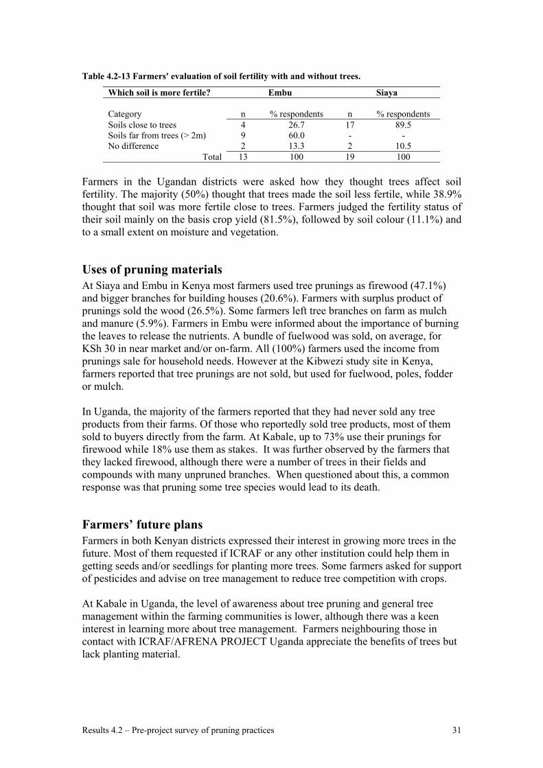
Results 4.2 – Pre-project survey of pruning practices 31
Table 4.2-13 Farmers' evaluation of soil fertility with and without trees.
Which soil is more fertile? Embu Siaya Category
n
% respondents
n
% respondents
Soils close to trees 4 26.7 17 89.5 Soils far from trees (> 2m) 9 60.0 - - No difference 2 13.3 2 10.5
Total 13 100 19 100 Farmers in the Ugandan districts were asked how they thought trees affect soil fertility. The majority (50%) thought that trees made the soil less fertile, while 38.9% thought that soil was more fertile close to trees. Farmers judged the fertility status of their soil mainly on the basis crop yield (81.5%), followed by soil colour (11.1%) and to a small extent on moisture and vegetation.
Uses of pruning materials At Siaya and Embu in Kenya most farmers used tree prunings as firewood (47.1%) and bigger branches for building houses (20.6%). Farmers with surplus product of prunings sold the wood (26.5%). Some farmers left tree branches on farm as mulch and manure (5.9%). Farmers in Embu were informed about the importance of burning the leaves to release the nutrients. A bundle of fuelwood was sold, on average, for KSh 30 in near market and/or on-farm. All (100%) farmers used the income from prunings sale for household needs. However at the Kibwezi study site in Kenya, farmers reported that tree prunings are not sold, but used for fuelwood, poles, fodder or mulch. In Uganda, the majority of the farmers reported that they had never sold any tree products from their farms. Of those who reportedly sold tree products, most of them sold to buyers directly from the farm. At Kabale, up to 73% use their prunings for firewood while 18% use them as stakes. It was further observed by the farmers that they lacked firewood, although there were a number of trees in their fields and compounds with many unpruned branches. When questioned about this, a common response was that pruning some tree species would lead to its death.
Farmers’ future plans Farmers in both Kenyan districts expressed their interest in growing more trees in the future. Most of them requested if ICRAF or any other institution could help them in getting seeds and/or seedlings for planting more trees. Some farmers asked for support of pesticides and advise on tree management to reduce tree competition with crops. At Kabale in Uganda, the level of awareness about tree pruning and general tree management within the farming communities is lower, although there was a keen interest in learning more about tree management. Farmers neighbouring those in contact with ICRAF/AFRENA PROJECT Uganda appreciate the benefits of trees but lack planting material.

Results 4.2 – Pre-project survey of pruning practices 32
Information on trees and their management at Mpigi
Fruit trees Artocarpus heterophyllus (Jackfruit) Found largely in a scattered arrangement, with a high tree density. It is reportedly competitive mainly for light, also for water. Shading of crops was the main reported problem. Mainly used domestically as fruit, also sold and used for fuel wood. The main forms of pruning are pollarding and side-pruning of branches, and the trees are pruned mainly when they shade crops. Carica papaya (Pawpaw): This was found in scattered arrangement. Exclusively used as fruit, mainly domestically, but also sold. Neither competition, nor any other problems were mentioned about it. It is never pruned. Citrus sinensis (Orange) This is planted in a scattered manner, inside homesteads. The majority of farmers visited did not have citrus on their farms. Competition with crops was not reported, and the trees are never pruned. Coffee This is scattered, but also planted in rows. It is used exclusively for cash, and pruned regularly to encourage emergence of vigorous coppices. Husbands do the pruning. Mangifera indica (Mango): Mainly scattered in homesteads. The main problem reported by farmers was shading of crops. It is pruned mainly by cutting a fraction of side branches, while a small fraction of farmers subject it to severe pruning. The pruning is done when trees shade crops. Persea americana (Avocado): This also is mainly found scattered. It is mainly planted but a small fraction regenerates naturally. Competition for moisture and light was reported. It is primarily grown for fruit (hom consumption and sale). No major problems were reported and pruning is done by cutting off a fraction of the side branches. Psidium guajava (Guava): Found in a scattered arrangement, this fruit tree was found on only 15% of the farmers’ plots visited. It is mainly planted, but also regenerates naturally. No problem was reported with the guava, and it is never pruned. Syzygium cuminii (Jambolan): This was a rare tree, for only 9.7% of the farmers visited had jambolan on their farms, where it exists in a scattered arrangement. It is mainly naturally regenerated but a few farmers planted their trees. Compared to the jackfruit whose density reached 10 trees per farm, jambolan density was only 1-2 tree per farm. Severe pruning is done and the tree reportedly competes with crops. Vangueria apiculata:

Results 4.2 – Pre-project survey of pruning practices 33
This was another rare tree, found on only 4% of the farms , where it was scattered within the farms. It is both planted and also regenerates naturally in a 1:1 ratio. Valued for its fruit, no major problems were reported with it. It is never pruned.
Timber trees Maesopsis eminii This is found scattered on the farms. It is valued mainly for timber, followed by fuel wood and shade. No major problems were reported about it, apart from competition with crops and slow growth. Only a small fraction of farmers reportedly prune Maesopsis (being self-pruning), by cutting off side branches. Milicia excelsa This is also found scattered, largely through natural regeneration. Valued for timber, competition with crops was not reported, and the tree is never pruned. It is not common on farmers’ plots (79.6% of farmers did not have it on their farms). Albizia: This was found in a scattered arrangement, with neither competition, nor any other problem reported. It is valued for soil conservation/fertility and shade. Not much pruning is done on it.
Others Markhamia lutea: This is mainly scattered, but also in lines around external boundaries. Mainly planted (46.3%) but also regenerates naturally (20.4%). The tree is planted by the majority of farmers interviewed. Competition for water was reported. It is planted primarily for poles, also firewood and wind breaks. Severe pruning is mainly done, followed by cutting of some branches. Some farmers pollard it. Largely husbands and children do the pruning. Ficus natalensis (Bark cloth tree): This is largely planted in a scattered arrangement (66.7%) and in lines (13%). It is solely planted from cuttings. It is mainly valued for firewood, shade and soil conservation, and bark cloth. The trees are regularly pruned, mainly by cutting side branches; pollarding and lopping are also done. The pruning is done when the trees shade crops, mainly by men and children. Sapium elipticum: This is found scattered on the farms and is almost exclusively naturally regenerated. It reportedly competes with crops for moisture and light. It is mainly kept for fuel wood and it is pruned by cutting a fraction of the branches. Spathodea campanulata: Found scattered on the farms, this tree multiplies through natural regeneration. Competition with crops for light was reported. It is valued largely for fuel wood. Competition with crops and slow growth were the major problems reported.

Results 4.5 – Root studies 34
4.3 Impacts of pruning on trees
4.3.1 Output 3. Effect of extreme crown pruning on large tree growth and survival
Sites in SW Uganda: Kalengyere, Bushenyi and Kachwekano (Experimental protocol no. 2) Previous survival and growth data from these studies is reported in Okorio et al., 1994 and Peden et al., 1996, 1997. During these previous studies, in 1994, the 5 central trees in each plot at Kalengyere, Bushenyi and Kachwekano were cut to ground level to assess biomass and pole production, leaving the 2 ‘guard’ trees at the end of each linear plot uncut. Since then, many of the cut trees had regrown as coppice. Data reported here cover both cut and uncut trees. None of these trials were guarded, and since the last evaluation, some trees had been cut illegally. Consequently, for some species ‘n’ is low and data should be treated with caution. At Kachwekano, Cedrela odorata and Markhamia lutea were originally planted at the site, but were omitted from this study because there were too few trees of these species remaining. Likewise at Kalengyere, Cedrela odorata and Albizia falcataria were omitted. Trees which had been previously cut in 1994 were about half the size of those which had not been cut and consequently, yielded much less biomass when pollarded in 1999. Survival of the pollarding treatment was good in all species at Kachwekano (Table 4.3-1), but at Kalenyere survival was less good for some species, especially for trees which had been cut previously in 1994 (Table 4.3-2), and survival of A. melanoxylon was especially poor. At Bushenyi, Acacia melanoxylon, Cedrela odorata, Cordia africana and Markhamia lutea which had been planted originally were all excluded from this study because of low plant numbers. Of the other species, the low numbers of previously uncut Eucalyptus grandis were due to unauthorised cutting (Table 4.3-3). Data obtained have been distorted to an extent by unauthorised cutting, which may be expected to target favoured species and large trees, though this may not necessarily be the case. Nevertheless, summary data (Figure 4.3-1) of all the species except those listed above, indicate that cutting five years previously reduced height and dbh, typically by about 50 %, and that a history of previous cutting reduced tree survival after pollarding. Previously cut trees produced substantial amounts of coppice regrowth (Figure 4.3-2) but the total biomass removed at pollarding was highest in the previously uncut trees. Of the trees which had not been previously cut, at Kachwekano, Eucalyptus yielded the highest biomass, followed by Grevillea, Albizia and Alnus, while at Kalengjere, Alnus was superior, followed by Eucalyptus. At Bushenyi, Casuarina glauca yielded most, followed by Grevillea.

Results 4.5 – Root studies 35
0.0
5.0
10.0
15.0
20.0
25.0
Kac
hwek
ano
Kal
engj
ere
Bus
heny
i
Kac
hwek
ano
Kal
engj
ere
Bus
heny
ipreviously cut previously uncut
0.0
20.0
40.0
60.0
80.0
100.0
120.0
Height in 1999 [m]dbh in Aug 99 (cm)dbh in Dec 2000 (cm)dbh in May 01 (cm)% survival after 1999
1.0
10.0
100.0
1000.0
Kac
hwek
ano
Kal
engj
ere
Bus
heny
i
Kac
hwek
ano
Kal
engj
ere
Bus
heny
i
previously cut previously uncut
Wt [kg] removed coppice atfirst pruning
Wt (kg) pollarded stem andside branches at firstpruningWt (kg) branches at secondpruning
Total biomass removed atfirst and second prunings
Figure 4.3-1 Mean tree height and dbh at 3 sites in SW Uganda where trees had previously been cut to the ground in 1994 (‘previously cut’), or not cut. All trees pollarded after measurements taken in 1999. (% survival on right hand axis)
Figure 4.3-2 Mean fresh biomass yielded by pollarding at sites in SW Uganda where trees had previously been cut to the ground in 1994 ('previously cut'), or not cut.

Results 4.5 – Root studies 36
Table 4.3-1 Growth, survival and biomass production (fresh mass) of trees at Kachwekano, planted in 1990, some of which were cut in 1994 for biomass and pole assessment (‘cut’), all of which were pollarded in 1999.
Tree Species Acacia
melanoxylon Albizia falcataria Alnus acuminata Casuarina
cunninghamiana Casuarina
glauca Eucalyptus
grandis Grevillea robusta Maesopsis eminii Polyscius fulva uncut cut uncut cut uncut cut uncut cut uncut cut uncut cut uncut cut uncut cut uncut cut No. trees before pollarding# 5 8 5 7 6 12 6 11 6 14 6 12 6 14 4 10 5 13No trees at end of study 5 8 5 7 6 12 6 11 6 14 6 12 6 14 4 8 4 13% survival after 1999 100 100 100 100 100 100 100 100 100 100 100 100 100 100 100 80 80 100Height in 1999 [m] 14.2 10.7 12.7 10.8 14.4 9.2 12.1 8.5 14.1 9.8 26.5 10.2 14.8 13.7 12.2 7.3 10.9 9.2Ht (m)of pollard cut 6.8 4.9 5.0 7.0 5.1 5.3 4.4 5.9 5.0 18.2 5.8 6.5 5.5 5.0 5.4 5.3 4.9dbh in Aug 99 (cm) 19.3 9.6 18.6 20.7 21.7 8.3 8.6 4.9 17.4 8.7 33.5 5.3 19.0 12.3 16.4 9.8 12.3 10.2dbh in Dec 2000 (cm) 21.5 9.0 18.3 11.2 28.3 10.9 12.2 5.4 15.4 8.0 41.9 9.2 18.8 14.0 20.2 11.7 17.8 9.5dbh in May 01 (cm) 22.1 10.1 mv* 12.0 29.0 12.3 12.7 5.7 15.7 8.8 43.4 10.4 24.0 13.3 20.9 12.1 18.7 10.2Wt [kg] removed coppice at first pruning 59.3 mv 15.3 14.0 75.0 1.0 9.8 0.0 27.4 0.0 15.8 1.0 117.5 0.0 11.9 11.2 70.2Wt (kg) pollarded stem and side branches at first pruning 141.3 9.9 229.6 * 215.6 22.9 4.8 64.9 10.1 637.3 22.1 236.7 31.5 100.5 23.0 108.5 *Wt (kg) branches at second pruning 3.9 13.7 12.7 * 52.3 32.5 1.9 3.4 3.8 4.7 37.7 33.4 17.9 15.2 16.4 7.9 12.9 13.4Biomass removed at first and second prunings 145.1 82.9 242.3 15.3 281.9 130.4 2.9 17.9 68.7 42.2 675.0 71.3 255.6 164.1 116.9 42.8 132.6 83.7# the original exptl plan allowed for 6 uncut and 15 cut trees * insufficient regrowth to merit repruning
first assessment and first pruning 26-Aug-
99
* missing value
second assessment (and second pruning)
1-Dec-00
third assessment 7-May-
01

Results 4.5 – Root studies 37
Table 4.3-2 Growth, survival and biomass production (fresh mass) of trees at Kalengyere, planted in 1990, some of which were cut in 1994 for biomass and pole assessment (‘cut’), all of which were pollarded in 1999.
Tree Species Acacia
melanoxylon Alnus acuminata Casuarina
glauca Casuarina
cunninghamiana Eucalyptus
grandis Polyscius fulva Grevillea robusta Markhamia lutea Melia azederach
uncut cut uncut cut uncut cut uncut cut uncut cut uncut cut uncut cut uncut cut uncut cut No. trees before pollarding 4.0 11.0 6.0 15.0 3.0 7.0 3.0 10.0 6.0 12.0 4.0 9.0 6.0 14.0 3.0 5.0 5.0 12.0No trees at end of study 3.0 4.0 6.0 15.0 3.0 5.0 3.0 10.0 6.0 12.0 4.0 7.0 6.0 14.0 3.0 5.0 5.0 9.0% survival after 1999 75.0 36.4 100.0 100.0 100.0 71.4 100.0 100.0 100.0 100.0 100.0 77.8 100.0 100.0 100.0 100.0 100.0 75.0Height in 1999 [m] 9.1 4.5 10.5 6.2 1.9 1.4 2.6 3.6 13.5 9.0 5.4 3.7 7.5 5.4 2.5 1.8 2.4 1.7Ht (m) of pollard cut (m) 7.0 3.4 6.7 4.0 2.5 1.8 4.4 3.1 7.8 6.0 4.3 3.9 4.8 4.7 3.7 2.6 1.8 1.7dbh in Aug 1999 (cm) 22.3 7.8 28.1 11.0 5.8 2.4 4.8 5.5 25.7 16.2 9.2 7.2 12.4 7.7 5.9 3.0 3.5 3.7dbh in Dec 2000 (cm) 25.4 9.7 29.4 11.1 0.0 3.1 4.2 6.1 24.1 14.2 11.1 9.8 13.5 9.5 7.0 3.5 4.2 3.9dbh in June 2001 (cm) 29.2 9.9 30.6 12.4 4.5 3.9 5.3 7.0 26.2 15.9 12.5 11.3 14.3 10.1 5.8 3.4 4.7 4.6Wt[kg] removed coppice at first pruning 0.0 31.5 46.0 45.0 0.0 0.4 0.0 2.9 0.0 19.7 9.8 25.7 65.7 23.5 2.0 0.6 6.0 1.9Wt(kg) pollarded stem and side branches at first pruning (kg) 91.5 18.6 283.3 18.2 5.4 0.6 8.0 6.1 169.0 61.6 3.3 2.4 53.8 14.5 2.2 0.3 1.5 0.9Wt(kg) branches at second pruning (kg) 0.0 1.2 78.3 39.6 0.7 0.5 1.7 2.1 45.3 26.7 11.7 18.9 15.3 9.5 3.8 1.5 1.5 1.3Biomass removed at first and second prunings 91.5 51.2 407.6 102.7 6.1 1.4 9.7 11.1 214.3 108.0 24.7 47.0 134.9 47.5 8.0 2.4 9.0 4.0
first assessment and first pruning 27-Aug-
99 second assessment (and second pruning)
5-Dec-00
third assessment 20-Jun-
01

Results 4.5 – Root studies 38
Table 4.3-3 Growth, survival and biomass production (fresh mass) of trees at Bushenyi, planted in 1990, some of which were cut in 1994 for biomass and pole assessment (‘cut’), all of which were pollarded in 1999. 1st assessment and pruning 31/8/99, 2nd assessment and pruning Dec 00, final assessment July 01.
Tree Species Albizia falcataria Alnus acuminata Casuarina
cuninghamiana Casuarina
cuninghamianaT5 Casuarina
equisetifolia(T6) Casuarina glauca(T2)
Casuarina glauca(T4)
Cedrela serrata(T5)
Cupressus lusitanica(T7)
uncut cut uncut cut uncut cut uncut cut uncut cut uncut cut uncut cut uncut cut uncut cut No. trees before pollarding 6.0 4.0 5.0 13.0 6.0 5.0 5.0 2.0 5.0 2.0 6.0 7.0 6.0 7.0 6.0 12.0 5.0 0.0No trees at end of study 6.0 3.0 3.0 9.0 6.0 1.0 4.0 2.0 5.0 2.0 5.0 6.0 6.0 2.0 4.0 4.0 3.0 0.0% survival after 1999 100.0 75.0 60.0 69.2 100.0 20.0 80.0 100.0 100.0 100.0 83.3 85.7 100.0 28.6 66.7 33.3 60.0 0.0Height in 1999 [m] 9.0 4.0 6.3 3.9 13.2 4.6 10.6 5.8 15.0 10.0 12.2 7.6 9.8 2.6 5.0 1.8 11.0 0.0Ht of pollard cut [m] 5.9 4.0 3.5 3.3 7.8 10.0 6.0 4.5 8.4 6.5 7.6 5.5 5.7 3.3 0.0 0.0 8.2 0.0dbh in Aug 1999 (cm) 15.1 6.9 9.9 4.8 23.4 10.2 10.2 5.4 22.0 1.3 21.0 6.1 12.1 1.1 9.3 2.7 30.4 0.0dbh in Dec 2000 (cm) 16.4 8.0 11.6 6.0 19.6 15.6 14.8 5.0 18.9 7.2 21.8 7.6 9.5 3.3 11.0 3.3 23.8 0.0dbh in July 2001 (cm) 16.5 9.2 11.8 6.2 20.3 16.0 15.1 5.0 17.7 9.2 22.2 8.9 10.2 3.7 12.2 4.2 23.8 0.0Wt [kg] removed coppice at first pruning 0.0 32.6 0.0 14.0 0.0 36.9 0.0 30.0 0.0 51.1 0.0 30.4 0.0 1.0 0.0 0.7 0.0 0.0Wt (kg) pollarded stem & side branches 1st pru 42.1 6.1 16.0 6.0 83.8 50.4 34.4 1.7 58.9 1.8 149.3 6.0 22.8 6.7 0.0 0.0 157.1 0.0Wt [kg] branches at second pruning 0.0 0.0 8.4 4.5 0.0 0.0 0.0 0.0 0.0 0.0 0.0 0.0 0.0 0.0 0.0 0.0 0.0 0.0Biomass removed at first and second prunings 42.1 38.7 24.4 24.5 83.8 87.3 34.4 31.7 58.9 52.8 149.3 36.4 22.8 7.7 0.0 0.7 157.1 0.0
Eucalyptus grandis(T8)
Grevillea robusta(T10R)
Grevillea robusta(T7)
Grevillea robusta(T8K)
Grevillea robusta(T9I)
Maesopsis eminii(T2)
Melia azedarach(T12)
Polyscius fulva(T3)
uncut cut uncut cut uncut cut uncut cut uncut cut uncut cut uncut cut uncut cut No. trees before pollarding 2.0 12.0 6.0 9.0 6.0 10.0 6.0 12.0 6.0 11.0 5.0 3.0 2.0 2.0 3.0 2.0 No trees at end of study 0.0 7.0 6.0 9.0 4.0 6.0 6.0 11.0 6.0 10.0 5.0 2.0 2.0 1.0 3.0 0.0 % survival after 1999 0.0 58.3 100.0 100.0 66.7 60.0 100.0 91.7 100.0 90.9 100.0 66.7 100.0 50.0 100.0 0.0 Height in 1999 [m] 4.0 9.1 10.1 7.0 11.2 7.5 13.0 7.2 12.9 7.7 10.0 5.5 4.4 2.3 8.3 2.5 Ht of pollard cut [m] 0.0 6.2 6.8 4.7 7.3 4.7 6.3 4.7 6.7 4.3 7.2 4.0 3.0 0.0 6.1 2.6 dbh in Aug 1999 (cm) 3.0 8.7 22.7 9.1 23.5 4.6 28.0 7.4 25.7 8.8 16.0 6.8 8.9 6.3 7.0 21.0 dbh in Dec 2000 (cm) 0.0 11.6 19.5 9.7 21.5 8.5 26.9 8.9 22.5 10.4 16.9 7.4 9.8 7.2 11.0 7.0 dbh in July 2001 (cm) 0.0 13.2 20.1 10.5 20.9 9.1 27.1 10.0 23.3 10.4 16.6 9.3 9.9 7.7 11.1 0.0 Wt [kg] removed coppice at first pruning 0.0 23.0 0.0 20.0 0.0 16.0 0.0 17.9 0.0 29.6 0.0 0.4 0.0 0.0 7.0 16.0 Wt (kg) pollarded stem & side branches 1st pru 0.0 20.2 111.4 13.0 145.0 10.4 275.4 10.2 169.9 12.5 49.5 5.7 26.0 0.0 11.5 3.8 Wt [kg] branches at second pruning 0.0 0.0 21.3 11.4 19.3 7.6 34.9 9.8 27.1 13.7 0.0 0.0 0.0 0.0 0.0 0.0 Biomass removed at first and second prunings 0.0 43.2 132.7 44.4 164.3 34.0 310.3 37.9 197.0 55.7 49.5 6.1 26.0 0.0 18.5 19.8

4.3 – Impacts of pruning on trees 39
Site at Mpigi, Uganda: Kabanyolo (Experimental protocol no. 2) At Kabanyolo, Alnus acuminata was excluded from the study because the trees were not considered large enough to be pollarded. Survival of Casuarina and Cupressus after pollarding was poor. Maesopsis and Cupressus yielded the largest amounts of biomass at pollarding (Table 4.3-4). Table 4.3-4 Biomass yield (fresh mass) at pollarding, and survival and sprouting pattern 6 months after pollarding at Kabanyolo, Uganda. Trees planted in 1988, pollarded in September 1999 and survival and regrowth assessed in April 2000.
Casuarina
equisetifolia Cordia
abyssinica Cupressus lusitanica
Maesopsis eminii
(Kakamega)
Maesopsis eminii
(Undanji) Markhamia
lutea Melia
azederach No. trees before pollarding 14.0 14.0 4.0 11.0 14.0 14.0 12.0No. trees at end of study 5.0 14.0 1.0 11.0 13.0 14.0 12.0% survival after pollarding 35.7 100.0 25.0 100.0 92.9 100.0 100.0Wt (kg) woody biomass removed at pollarding 88.3 107.1 119.9 217.9 201.9 122.1 167.5Wt. (kg) leafy biomass removed at pollarding 18.3 17.5 98.5 27.0 26.9 20.1 27.6Total biomass removed (kg) 106.5 121.8 218.4 244.9 228.7 143.4 195.0Length of bole covered in sprouts (cm) 396.2 415.6 160.0 360.7 365.0 414.6 439.1No. of sprouts 38.6 18.5 18.0 12.0 10.5 15.1 32.9
Siaya, Kenya (Experimental protocol no. 5) (Plate 2-Plate 5) At Siaya, two species, Cedrela odorata and Alnus acuminata were excluded from the study due to their poor growth rate. Survival of the remaining four species (Casuarina equisetifolia, Eucalyptus grandis, Grevillea robusta and Markhamia lutea) was excellent, close to 100%, irrespective of pruning treatment, although some Eucalyptus and Markhamia were lost due to unauthorised cutting. However, effects of treatment on growth rate started to become apparent two years after pruning (Table 4.3-5, Figure 4.3-3), so that unpruned trees tended to have the largest dbh values and trees receiving crown pruning or combined crown and root pruning tended to be smallest. Grevillea, Casuarina and Markhamia were less affected by root pruning than by treatments involving crown pruning, and Grevillea was the species which was most sensitive to crown pruning.

Results 4.5 – Root studies 40
Table 4.3-5 Effect of pruning treatment on dbh of trees at Siaya, Kenya. Trees were pruned in March 99 at 48 months old and crown pruning was repeated in Aug 99, Feb 02 and Oct 02. (letters indicate significant differences between pruning treatments within a species at a particular time)
Species Pruning Treatment Mar 99 Dec 99 Feb 01 Feb 02 Oct 02 % of
unprunedCasuarina crown pruned 14.4a 14.6a 16.1a 15.6b 16.9c 75 root pruned 13.2a 15.9a 17.6a 17.0b 21.0b 93 crown and root pruned 13.4a 13.9a 15.2a 15.9b 16.5c 73 not pruned 12.6a 15.8a 17.9a 21.5a 22.5a 100Eucalyptus crown pruned 18.3a 21.2a 22.8a 20.4a 27.7b 81 root pruned 15.8b 21.5a 19.6b 19.9a 24.0b 70 crown and root pruned 19.8ab 21.0a 22.8a 20.5a 25.4b 74 not pruned 17.2ab 20.9a 24.0a 23.8a 34.3a 100Grevillea crown pruned 10.0a 10.7cb 11.6b 12.9cb 13.4b 69 root pruned 10.7a 12.8ab 14.5ab 15.2ab 19.0a 98 crown and root pruned 9.2a 9.5c 12.5b 10.8c 11.2b 58 not pruned 11.4a 14.1a 15.5a 16.8a 19.4a 100Markhamia crown pruned 7.8a 8.6a 10.4a 12.7ab 13.2bc 89 root pruned 7.6a 9.2a 10.4a 12.4ab 13.8b 93 crown and root pruned 6.8a 7.6a 8.9a 10.1b 10.8c 73 not pruned 8.0a 10.2a 11.5a 13.1a 14.8a 100 Although the dbh of crown and combined crown and root pruned treatments were not significantly different within a species, there are strong indications that pruned biomass was affected (Table 4.3-6). Combined crown and root pruning yielded less biomass than crown pruning on its own.

Results 4.5 – Root studies 41
Figure 4.3-3 Effects of pruning treatment on diameter at breast height (cm) of tree species at Siaya, Kenya (note Eucalyptus on different scale)
Casuarina equisetifolia
0.0
5.0
10.0
15.0
20.0
25.0
Mar 99 Dec-99 Feb-01 Feb-02 Oct-02
crow n pruned
root pruned
crow n and root pruned
not pruned
Eucalyptus camaldulensis
0.0
5.0
10.0
15.0
20.0
25.0
30.0
35.0
40.0
Mar 99 Dec-99 Feb-01 Feb-02 Oct-02
Grevillea robusta
0.0
5.0
10.0
15.0
20.0
25.0
Mar 99 Dec-99 Feb-01 Feb-02 Oct-02
M arkhamia lutea
0.0
5.0
10.0
15.0
20.0
25.0
Mar 99 Dec-99 Feb-01 Feb-02 Oct-02

Results 4.5 – Root studies 42
Table 4.3-6 Biomass (air dry) yielded by different pruning treatments at Siaya, Kenya. First pruning was done when trees were 48 months old, and trees then repruned at 53, 83 and 91 months.
kg 'stems+twigs+leaves' Mar 99 Aug 99 Feb 02 Oct 02 month 48 53 83 91 Total biomassCasuarina crown 31.5 2 45 1.5 80.0 crown + root 31.5 2 38 2.0 73.5Eucalyptus crown 107 10 120 12.7 249.7 crown + root 107 10 75 8.2 200.2Grevillea crown 18 3 38 1.9 60.9 crown + root 18 3 23 1.9 45.9Markhamia crown 5.5 4 23 2.5 35.0 crown + root 5.5 4 17 1.4 27.9
Time taken to prune The amount of time taken for tree pruning varied according to species, reflecting the size of the trees (Table 4.3-7). Root pruning was much more time consuming than crown pruning. At this site, root pruning was done in a circle around the tree base, which was awkward to do in dry ground with the tools available. Table 4.3-7 Time taken for tree pruning at Siaya, western Kenya (first pruning, at 48 months after planting).
Species Time taken (minutes/tree)1 Crown Root Total Casuarina equisetifolia 14c 85b 99b Eucalyptus grandis 30a 96a 126a Grevillea robusta 20b 77c 97b Markhamia lutea 6d 44d 50c Prob > F-ratio 0.0001 0.0001 0.0001 Lsd2 3.13 7.30 8.22 1Values in the same column followed by different letters are significantly different (P < 0.05). 2Lsd = Least significant difference.
Results 4.5 – Root studies 43
Plate 1 Pruning of Grevillea trees as practised by farmers at Embu (not part of the project). Many boundary trees are pruned. Projecting side branches are left to provide access for climbing. Cut branch stumps on main bole are undesirably long.

Results 4.5 – Root studies 44
Plate 2 Tree regrowth after the first pruning at Siaya. A good maize crop was produced after pruning

Results 4.5 – Root studies 45
Plate 3 Repruning at Siaya in February 2002. Regrowth after the previous pollarding has been cut at the original pollarding height.

Results 4.5 – Root studies 46
Plate 4 Eucalyptus poles cut at Siaya in February 2002 from the pollarding regrowth

Results 4.5 – Root studies 47
Plate 5 Regrowth of Casuarina and Eucalyptus in June 2002, after repruning in February 2002. Casuarina tended to produce regrowths more slowly than other species at this site.
4.3.2 Output 4 Impacts of pruning on young (small) trees While work under output 3 examined the effects of pruning large trees, the impacts of pruning of young trees is also important as tree-crop competition sets in early in many agroforestry systems. Studies at Kifu 1 examined effects of different crown pruning techniques on tree growth, while studies at Kifu 2 and Nyabeda evaluated root pruning on one side of tree rows. On farm experimentation at Kabale (output 6) evaluated crown and combined crown and root pruning. The characteristics of the study sites are as Table 3.1-2 Other pruning study sites: early crown pruning at Kifu 1 and root pruning at Kifu 2 and Nyabeda. . At Siaya, root pruning in a ring around the tree was evaluated, whereas at Nyabeda, Kifu and Kabale, the more straight forward approach of root pruning in a straight line along one side of a row of trees was evaluated.
Kifu 1, Uganda (Experimental protocol no. 4) At Kifu, intensity of crown pruning significantly affected tree dbh and height (p<0.001) at both 2 and 4 years after the first pruning (Table 4.3-8).

Results 4.5 – Root studies 48
Table 4.3-8 Effect of intensity of crown pruning on dbh and height (cm) of trees at Kifu 1, 2 and 4 years after first pruning.
Un-pruned 1/3 pruned 2/3 pruned Pollarded
2 years after first pruning dbh ht dbh ht dbh ht dbh ht Cordia 11 498 9.4 403 8.5 346 9 266 Grevillea 8.1 566 7.8 571 5.8 502 5.8 317 Senna 9.3 464 7.2 604 7.4 593 7.1 592 4 years after first pruning Cordia 14.5 1080 11.9 727 10 539 11.5 330 Grevillea 15.3 1203 14.5 1123 11.2 982 8.4 338 Senna 12.9 1223 11.7 1107 11.2 957 11 893
Effects of pruning were apparent at the first measurement, 2 years after pruning. All species were affected, and growth was reduced most with the more severe treatments. Generally, Senna appears less affected by treatment severity.
Kifu 2, Uganda (Experimental protocol no.2) At Kifu, significant main effects of root pruning on tree dbh and height occurred. The effect on dbh became apparent 13 months after pruning (Table 4.3-9). Species x pruning interactions were not significant, and pruning reduced the dbh of Casuarina, Grevillea, Maesopsis, Alnus and Markhamia by 12, 5, 6, 10, and 4% respectively.
Table 4.3-9 Effects of root pruning on DBH (cm) at Kifu 2 (averaged over the different species) over the study period.
Months after planting 43 50 56 60 63 66 69
Pruned trees 9.5 11.8 13.1 13.7 14.1 14.5 15.4
Un-pruned trees 9.9 12.4 13.9 14.5 15.1 15.6 16.5
SED 0.67 0.51 0.41 0.39 0.40 0.42 0.43
P 0.60 0.26 0.06 0.04 0.02 0.02 0.02
In this trial, where crown pruning was not imposed, significant main effects of root pruning on tree height were also observed, from 13 months after the first pruning (Table 4.3-10). Species x pruning interactions were not significant, and the heights of Casuarina, Grevillea, Maesopsis, Alnus and Markhamia were reduced by 8, 0, 9, 3, and 4% respectively.

Results 4.5 – Root studies 49
Table 4.3-10 Effects of root pruning on height (m) of trees at Kifu 2 (averaged over the different species) during the period when pruned and un-pruned trees were significantly different in height.
Months after planting 56 60 63 66 69 Pruned trees 10.6 11.5 12.0 12.3 12.8 Un-pruned trees 11.0 11.9 12.5 12.9 13.3 SED 0.21 0.23 0.23 0.24 0.25 p 0.05 0.06 0.03 0.02 0.04
No adverse effects of pruning on survival of any of the species were observed.
Nyabeda, Kenya (Experimental protocol no. 6) Tree growth at Nyabeda was measured before pruning and 12 months later. Before pruning, there was no significant difference between the groups of trees allocated to the different pruning treatments. Twelve months later, there was still no significant difference in height or dbh. However, whereas unpruned trees had gained 0.5 m in height, the pruned trees were the same height as 12 months previously. Trees in both treatments had made similar increases in stem diameter (Table 4.3-11). All trees survived the experimental treatments. Table 4.3-11 Growth of Grevillea robusta at Nyabeda, Kenya, determined at 72 months after planting, before pruning was imposed, and 12 months later. Pruned trees had been root pruned along one side of the tree row.
Months after planting 72 months 84 months Height (m) Pruned trees 12.9 12.9 Unpruned trees 13.2 13.7 SED 0.33 0.55 P 0.483 0.271 DBH (cm) Pruned trees 13.5 15.5 Unpruned trees 14.0 15.9 SED 0.47 0.24 P 0.347 0.171
4.3.3 Output 6. On farm experimentation in Uganda (Experimental protocol no. 1)
In this study, Grevillea robusta and Alnus acuminata, planted in farmers’ fields in 1994, were pruned, 5 years later, in 1999, and repruned two years later in 2001. Pollarding and combined pollarding and root pruning were compared against unpruned controls. Significant effects of pruning treatment on dbh were apparent from 10 months after the first pruning. Growth of both species was reduced by pruning and both treatments reduced growth to the same extent . No significant effects of species or pruning treatment were found on pruning biomass Figure 4.3-4). At the first pruning, pollarding and side pruning produced about 22 kg

Results 4.5 – Root studies 50
fresh biomass of twigs and branches and the second pruning, 2 years later, produced about 12 kg (Table 4.3-12). No effects of pruning treatment on survival were observed.
LSD
10
11
12
13
14
15
16
0 10 20
Months after pruning
DB
H (c
m)
pollarded
pollarded and rootprunednot pruned
Table 4.3-12 Crown biomass (branches and twigs, kg per tree) removed during pruning of Alnus and Grevillea trees planted at Kabale, Uganda. Trees were planted in 1995 and were first pruned (T0) in 1999 at 4 years of age, second crown pruning was 24 months later (T24). P1 = pollarding, P2 = pollarding and root pruning on one side of the tree row.
Mean of Grevillea and Alnus P1 P2
Fresh mass T0 21.3 24.5 Dry mass T0 10.2 11.9 Fresh mass T24 12.8 12.1 Dry mass T24 6.2 5.9
Prior to this study, trees had been lightly managed by farmers to remove low branches, which interfered with crops. At five years of age, when this study started, Alnus was taller than Grevillea and had greater volume. This is not reflected in the biomass removed at first pruning because some Alnus were of sufficient length to yield two logs and proportionately less material was removed, so both tree species yielded similar amounts of biomass from the pollarding and side pruning, and repruning 24 months later yielded about half the original amount. Farmers judged the prunings to be useful as stakes, especially for climbing beans, which are an important local crop, and fuel. In a study in the same locality (David and Raussen 2003), farmers considered that firewood from 2-year old Alnus acuminata from a rotational fallow was superior to locally produced Eucalyptus. Alnus acuminata and Grevillea robusta have similar calorific values (19250 kJ kg-1 and 19460 kJ kg-1) (CATIE 1986; Jain and Singh 1999).
Figure 4.3-4 Effects of pollarding and root pruning on tree diameter at breast height (cm). Trees were 63 months old at the time of first pruning. Data for Grevillea and Alnus combined. Bar is LSD between treatments at a particular time.

Results 4.5 – Root studies 51
Household wood fuel use in Uganda has been estimated at 2.18 kg/cap/day (Yevich and Logan, in press) and a family meal can be cooked with 1.6 kg of wood (14 % moisture content) on a sheltered 3-stone stove, with lidded cooking pot (George, 2002). These two figures give somewhat different impressions of daily household use, but this is highly variable and there are many strategies for reducing consumption when resources are scarce. Based on the above stove measurements, and making an allowance of 10 % for wastage, each tree at first pruning would cook about 8 family meals and at second pruning would provide fuel for about four family meals.
Potential wood production on farm With an average land holding of 2.06 ha, assuming an average terrace width of 10 m (Siriri, pers. com.), a household would have approximately 2000 m of terrace edge available, on which 1000 trees could be planted at 2 m spacing. If 200 trees were planted in each of the first 5 years, and first and second cuts followed the pattern adopted in this study, the trees would start to yield significant quantities of wood at year 5, and from the seventh year onwards, yields of 2500 – 4500 kg per farm per year would be achieved, which should meet most domestic fuel requirements. Additionally, the trunk would be available for harvest when the farmer required. The long term productivity of such a system is a matter for speculation as the tree’s response to repeated cutting is not known. Trunk increment has already been reduced by the pruning treatments. The vigour with which trees will continue to regrow after pollarding is likely to be influenced by pruning frequency. When coppicing, Sims et al. (1999) found that mortality of several Eucalyptus species increased with successive harvests, and Hytönen and Issakainen (2001) found that frequency of coppicing of Betula pubescens affected biomass production and the species’ ability to resprout. Pollarding removes the same amount of photosynthetic material as coppicing, but less woody material, which should leave greater carbohydrate reserves for regeneration, and it allows a mature trunk to be harvested at the end of the rotation. In this pollarding study, tree survival was excellent and unaffected by treatment. Compared with the first cut when coppicing, pollarding wounds will be of smaller diameter and should recover more quickly, and regrowth from pollarding will be less damaged by uncontrolled grazing as sprouts will be out of reach of animals. Compared with felling and replanting, the pollarding system has lower establishment and maintenance costs – new plants do not have to be produced, weeded, or protected from animals, and a long knot-free trunk should be produced. A negative aspect of pollarding is that the trees must be climbed or ladders used, which requires training. On a per tree basis, labour requirements for pruning are small (Table 4.3-7), but as the number of trees per farm increases, it could impinge on other activities, but families must obtain wood from somewhere, and the availability of a steady fuel supply on farm is regarded as an asset by many households. Pruning in this study was conducted in the dry season, when land beneath the trees was clear of crops and when trunks were not slippery. While women felt that root pruning could be easily tackled as part of the land

Results 4.5 – Root studies 52
preparation process, they preferred to leave any crown pruning which involved tree climbing to male members of their families.
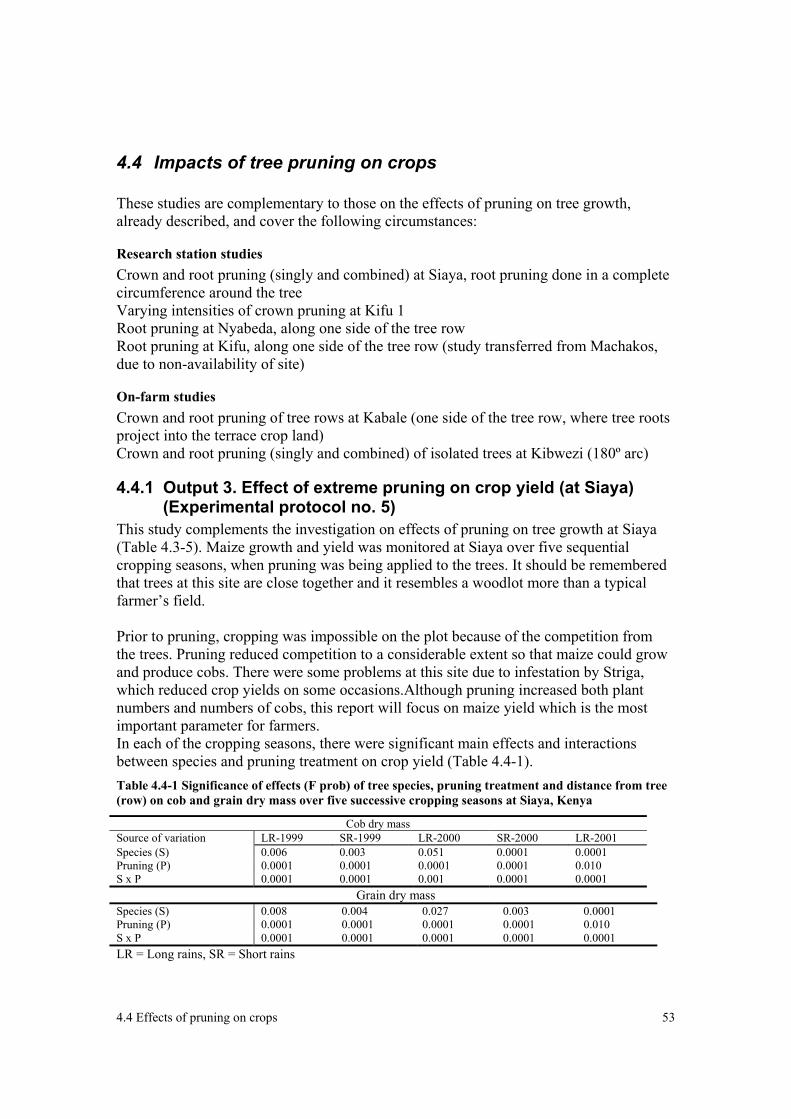
4.4 Effects of pruning on crops 53
4.4 Impacts of tree pruning on crops These studies are complementary to those on the effects of pruning on tree growth, already described, and cover the following circumstances:
Research station studies Crown and root pruning (singly and combined) at Siaya, root pruning done in a complete circumference around the tree Varying intensities of crown pruning at Kifu 1 Root pruning at Nyabeda, along one side of the tree row Root pruning at Kifu, along one side of the tree row (study transferred from Machakos, due to non-availability of site)
On-farm studies Crown and root pruning of tree rows at Kabale (one side of the tree row, where tree roots project into the terrace crop land) Crown and root pruning (singly and combined) of isolated trees at Kibwezi (180º arc)
4.4.1 Output 3. Effect of extreme pruning on crop yield (at Siaya) (Experimental protocol no. 5)
This study complements the investigation on effects of pruning on tree growth at Siaya (Table 4.3-5). Maize growth and yield was monitored at Siaya over five sequential cropping seasons, when pruning was being applied to the trees. It should be remembered that trees at this site are close together and it resembles a woodlot more than a typical farmer’s field. Prior to pruning, cropping was impossible on the plot because of the competition from the trees. Pruning reduced competition to a considerable extent so that maize could grow and produce cobs. There were some problems at this site due to infestation by Striga, which reduced crop yields on some occasions.Although pruning increased both plant numbers and numbers of cobs, this report will focus on maize yield which is the most important parameter for farmers. In each of the cropping seasons, there were significant main effects and interactions between species and pruning treatment on crop yield (Table 4.4-1). Table 4.4-1 Significance of effects (F prob) of tree species, pruning treatment and distance from tree (row) on cob and grain dry mass over five successive cropping seasons at Siaya, Kenya
Cob dry mass Source of variation LR-1999 SR-1999 LR-2000 SR-2000 LR-2001 Species (S) 0.006 0.003 0.051 0.0001 0.0001 Pruning (P) 0.0001 0.0001 0.0001 0.0001 0.010 S x P 0.0001 0.0001 0.001 0.0001 0.0001
Grain dry mass Species (S) 0.008 0.004 0.027 0.003 0.0001 Pruning (P) 0.0001 0.0001 0.0001 0.0001 0.010 S x P 0.0001 0.0001 0.0001 0.0001 0.0001 LR = Long rains, SR = Short rains

Results 4.5 – Root studies 54
In the absence of pruning, yields were very low. Tree pruning had beneficial effects on crop yield (Table 4.4-2). Generally, crown pruning or combined crown and root pruning were more beneficial than root pruning. Root pruning alone was particularly ineffective for Casuarina. Although root pruning would be expected to displace tree root activity below the cropping zone, the beneficial effects of this may only be realized if the dense crown canopy, which intercepts rain, is removed or reduced. Table 4.4-2 Effects of tree pruning treatments on maize cob yield (dry mass) (kg/ha) over five cropping seasons at Siaya, western Kenya. Trees were pruned in March 99 at 48 months old (just before the first cropping season) and crown pruning was repeated in Aug 99 (before the second cropping season). Further repruning was not done until after completion of the cropping study.
Treatments Cropping seasons Long rain
1999 Short rain 1999
Long rain 2000
Short rain 2000
Long rain 2001
Casuarina equisetifolia Crown pruning 770.6b 2578.7a 437.7b 468.4b 738.8b Root pruning 211.2c 1045.9c 76.1c 252.81c 287.4c Crown + Root 887.2a 2554.5a 760.2a 708.3a 866.7a Control 255.0c 1546.8b 122.0c 312.3c 349.6c Lsd 70.5 159.9 74.4 68.1 66.8 Sole maize 781.2 2263.4 1494.6 944.1 1036.8 Eucalyptus grandis Crown pruning 1547.8a 2699.8a 419.0c 573.8b 874.6b Root pruning 732.9c 2121.1b 783.5a 670.8a 1119.8a Crown + Root 1010.6b 2338.7b 536.0b 559.7b 799.5c Control 166.5d 898.1c 158.4d 393.4c 924.2b Lsd 154.7 212 100.4 94.0 74 Sole maize 781.2 2263.4 1494.6 944.1 1036.8 Grevillea robusta Crown pruning 602.6b 1788.3b 539.9b 502.8b 727.8b Root pruning 982.1a 1702.2b 327.2c 301.9c 683.4b Crown + Root 621.5b 2361.9a 719.8a 906.1a 911.3a Control 360.8c 1397.9c 240.1d 298.8c 608.2c Lsd 101.8 155.0 73.0 55.3 82.2 Sole maize 781.2 2263.4 1494.6 944.1 1036.8 Markhamia lutea Crown pruning 990.8a 2657.8a 707.8a 590.3b 845.8b Root pruning 841.1a 1931.4b 506.6b 598.8b 1040.3a Crown + Root 553.7b 2725.2a 643.9a 602.2b 1016.8a Control 226c 1874.0b 298.1c 804.8a 895.2b Lsd 168.1 168 101.8 76.2 105.2 Sole maize 781.2 2263.4 1494.6 944.1 1036.8 Lsd = Least significant difference; for each species, values in the same column followed by different letters are significantly different (P < 0.05). Shortly after the first pruning, 15 % more rain was collected in rain gauges at ground level on crown pruned, compared with unpruned plots. One year later, as crowns regrew, 7 % more rain was collected and by late 2001, there was no difference in collected rainfall amount.

Results 4.5 – Root studies 55
Crop yield on tree plots receiving different pruning treatments relative to plots without trees is summarised in Figure 4.4-1. Pruning improved crop yields, especially during the first two seasons after pruning, and often resulted in crop yields similar or greater than those of plots without trees. Crops with Casuarina were unresponsive to root pruning on its own. Effects of other trees were variable according to season and time since pruning. There are indications that combined crown and root pruning was more effective and long lasting than crown pruning alone and that root pruning alone was less effective than treatments which included crown pruning. Crops growing with Eucalyptus were most responsive to pruning. The corresponding soil water studies (Figure 4.6-3, Figure 4.6-4) showed that combined crown and root pruning improved soil water amounts relative to the other pruning treatments, but did not eliminate the effects of trees on soil water. Extent of root regrowth was assessed on a subset of trees in February 2001 (Table 4.5-1). Root regrowth of Eucalyptus was significantly less than that of the other species.

Results 4.5 – Root studies 56
Figure 4.4-1 Effects of different pruning methods on yields of crops grown with different tree species, expressed as a % of crop growth without trees. (LR = long rains, SR = short rains)
Casuarina equisetifolia
0
50
100
150
200
250
LR1999
SR1999
LR2000
SR2000
LR2001
Grevillea robusta
0
50
100
150
200
250
LR1999
SR1999
LR2000
SR2000
LR2001
Eucalyptus grandis
0
50
100
150
200
250
LR1999
SR1999
LR2000
SR2000
LR2001
Markhamia lutea
0
50
100
150
200
250
LR1999
SR1999
LR2000
SR2000
LR2001
Crown pruningRoot pruningCrown + Root pruningsControl (not pruned)
Gra
in d
wt a
s % o
f sol
e m
aize
Maize cropping season
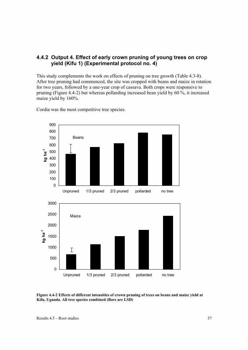
Results 4.5 – Root studies 57
4.4.2 Output 4. Effect of early crown pruning of young trees on crop yield (Kifu 1) (Experimental protocol no. 4)
This study complements the work on effects of pruning on tree growth (Table 4.3-8). After tree pruning had commenced, the site was cropped with beans and maize in rotation for two years, followed by a one-year crop of cassava. Both crops were responsive to pruning (Figure 4.4-2) but whereas pollarding increased bean yield by 60 %, it increased maize yield by 160%. Cordia was the most competitive tree species.
0
100
200
300
400
500
600
700
800
900
Unpruned 1/3 pruned 2/3 pruned pollarded no tree
kg h
a-1
Beans
Figure 4.4-2 Effects of different intensities of crown pruning of trees on beans and maize yield at Kifu, Uganda. All tree species combined (Bars are LSD)
0
500
1000
1500
2000
2500
3000
Unpruned 1/3 pruned 2/3 pruned pollarded no tree
kg h
a-1
Maize

Results 4.5 – Root studies 58
When cassava was grown (Figure 4.4-3), Cordia and Senna were most competitive and the greatest crop responses to pruning were found with these species. With Grevillea, increasing pruning to > 1/3 of crown did not confer benefits on crop yield, whereas maximum yield with Cordia and Senna was achieved with 2/3 crown pruning.
This is the only site at which cassava was grown, and at which a wider range of crown pruning treatments was tested. These results indicate that to maximise yields of some crops, in some environments, extreme crown pruning may be unnecessary and an intermediate intensity of pruning, which will be more advantageous to tree growth, may be suitable. This will depend upon water availability, light requirements and irradiance at different sites.
4.4.3 Output 5. Effect of root pruning on crop growth (Kifu 2 & Nyabeda) (Experimental protocol nos. 3 & 6)
Kifu Crops were planted at Kifu as follows
• In April 1999, 2 months after the first root pruning (maize) • In December 1999, 1 month after the second root pruning (beans) • In May 2000, 6 months after the second root pruning (maize) • In November 2000, immediately after the third root pruning (beans) • In June 2001, 7 months after the third root pruning (maize)
Figure 4.4-3 Effects of tree species and pruning intensity on yield of cassava at Kifu, Uganda
0
5
10
15
20
25
30
35
Control Cordia Grevillea SennaCas
sava
tube
r yi
elds
(Kg/
10
m r
ow)
Zero pruning1/3 crown pruning2/3 crown pruningPollarding of crown

Results 4.5 – Root studies 59
For brevity, this report will focus on the last 3 crops. Full details of the experimental design are provided in the Experimental Protocol. Crop production is considered in two ways: A. in terms of the pruning treatment received by the trees at the tree plot level, combining crop growth from both sides of trees: TP1 = root pruned one side TP2 = not root pruned (see Figure 4.4-4) B. In terms of the side of the tree on which the crop was growing
P1 = root pruned plot, the side of the tree where root pruning was done P2 = unpruned plot (measured on the same side of the tree row as P3) P3 = root pruned plot, the side of the tree where root pruning was not done. (see Figure 4.4-5)
Figure 4.4-4 Location of the tree root pruning subplots at Kifu – ‘pruning’
TP1
TP2

Results 4.5 – Root studies 60
Maize yield in the first cropping season on 2000 This crop was sown when the trees were 56 months old, 6 months after the second root pruning. Significant effects of tree species and ‘side’ occurred up to 4.5 m from the tree for the former, and up to 7.5 m from the tree for the latter (Table 4.4-3). Note the lack of effect of ‘pruning’, which will be investigated further. Table 4.4-3 Significance of effects of species, 'pruning' and 'side' on maize grain yield at different distances from the tree rows in 2000, sown 6 months after second root pruning
1.5 m 3.0 m 4.5 m 6.0m 7.5 m 9.0 m Species 0.018* 0.004** 0.008* 0.085 0.337 0.357 Pruning 0.773 0.177 0.790 0.210 0.944 0.612 Sp x pruning 0.625 0.993 0.556 0.664 0.602 0.572 Side 0.008* <.0.001*** 0.002** 0.003** 0.013* 0.218 Species x Side 0.995 0.680 0.390 0.287 0.946 0.950
Overall, Grevillea was the least competitive species close to the trees (Table 4.4-4).
Table 4.4-4 Effect of tree species on maize grain yield (kg /pair of 6m rows) at different distances from tree plots for the 2000 maize crop (pruned and unpruned treatments combined)
Species 1.5 m 3.0 m 4.5 m 6.0 m 7.5 m 9 m Casuarina 1.6b 3.0b 4.1bc 5.3 6.2 6.9 Grevillea 3.9a 4.0a 4.6b 5.0 5.4 5.8 Maesopsis 2.4b 2.8b 3.9b 5.0 5.8 5.9 Alnus 2.7b 4.6a 5.6a 5.9 6.1 6.1 Markhamia 2.8ab 3.0b 3.5c 4.9 5.7 6.3 No tree = 6.4 SED 0.6 0.4 0.5 0.4 ns 0.4 ns 0.6 ns
* Numbers with same letters within a column are not significantly different
Figure 4.4-5 Location of the pruning sub-sub plots at Kifu, relative to the ‘side’ of the tree
Tree row Line of root pruning
P1
P2
P3

Results 4.5 – Root studies 61
When effects of pruning ‘side’ were examined (Table 4.4-5), the yield of crops on the side where root pruning had been applied (P1) was significantly greater than the other treatments, and the effects of root pruning extended up to 7.5 m from the trees. However, the yield on P3, the plot on the unpruned side of the pruned trees, was the lowest of all three treatments although the root system would be expected to be similar in quantity and extent to that on the P2 plot.
Table 4.4-5 Effects of 'side' (Figure 4.4-5) on maize grain yield (kg/pair of 6 m row) at different distances from the tree line (all tree species combined) for the 2000 maize crop
Pruning ‘side’ 1.5 m 3 m 4.5 m 6 m 7.5 m 9 m P1 2.4a 3.2a 4.0a 4.6a 4.9a 4.9 P3 1.6c 2.0c 2.5c 3.3c 3.9b 4.3 P2 2.0b 2.6b 3.3b 3.9b 4.4ab 4.6 SED 0.19 0.20 0.29 0.28 0.28 0.32
* Numbers with same letters within a column are not significantly different This pattern of P1 >P2>P3 was consistent across all tree species (Table 4.4-6). As at Siaya, crop yield with Casuarina was relatively poor. Although crops planted with it showed a substantial response to root pruning, yields remained lower than with other tree species. Table 4.4-6 Maize yields (kg / pair of 6 m rows) on different ‘sides’ (Figure 4.4-5), and at different distances from the tree line during the maize cropping season in 2000
Distance 1.5 m 3.0 m 4.5 m 6.0 m 7.5 m 9.0m P1 Casuarina 1.7 3.1 4.2 4.7 5.1 5.7 Grevillea 3.2 3.4 4.1 4.4 4.6 4.9 Maesopsis 2.2 2.7 3.7 4.4 5.0 4.3 Alnus 2.4 3.7 4.1 4.3 4.7 4.8 Markhamia 2.5 2.9 3.9 5.1 5.1 5.0 P3 Casuarina 0.7 1.4 2.0 3.3 4.2 4.7 Grevillea 2.7 2.6 2.8 3.1 3.5 3.8 Maesopsis 1.3 1.4 2.3 3.1 3.7 4.5 Alnus 1.7 3.2 4.2 4.5 4.4 4.3 Markhamia 1.7 1.5 1.4 2.2 3.5 4.4 P2 Casuarina 1.2 2.2 3.1 4.0 4.6 5.2 Grevillea 3.0 3.0 3.4 3.7 4.0 4.3 Maesopsis 1.8 2.1 3.0 3.7 4.4 4.4 Alnus 2.0 3.5 4.2 4.4 4.6 4.5 Markhamia 2.1 2.2 2.7 3.7 4.3 4.7 SED 0.5 0.5 0.6 0.6 0.6 0.7
Overall, the effects of P1 and P3 are illustrated in Plate 6.

Results 4.5 – Root studies 62
While there was a significant effect of ‘side’, the effects of ‘pruning’ were not significant. Similar effects were also observed in other cropping seasons. These results indicate that the gains in crop yield from root pruning on one side of the trees were offset by losses in crop yield on the opposite side of the same trees, presumably arising from increased root activity on the unpruned side of the trees.
Nyabeda Studies at Nyabeda focussed on Grevillea. Root pruning had a significant effect on crop yield for the first two seasons and fourth season after pruning. However, whereas the results at Kifu clearly indicated redirection of root activity after root pruning, the results at Nyabeda do not show this (Table 4.4-7). In the first season after root pruning, when effects would be expected to be strongest, the yields from P1 and P3 were higher than from P2. In the following season (Long rains 2000), P1 was higher than P3 and P2, and in the short rains 2000, no effects were observed. Referring back to the Kifu study, it is evident that Grevillea was the least competitive of all the species studied (Table 4.4-6), even though it was one of the largest species.
Plate 6 ‘Side’ effects of root pruning on growth of maize with Maesopsis at Kifu. P1 is on the left, and P3 on the right

Results 4.5 – Root studies 63
Table 4.4-7 Maize yield at Nyabeda, after root pruning of Grevillea prior to the short rains of 1999
Treatments
Cropping seasons
Short rain 1999 Long rain 2000 Short rain 2000 Cob dry mass kg / ha
One side root pruned ‘P1’
476.0b 924.6b 591.9a
The other side un-pruned ‘P3’
504.3b 783.9c 602.2a
Both sides un-pruned control ‘P2’
353.8c 743.1c 621.2a
Sole maize 674.7a 1013.0a 611.3a Lsd 58 62.8 59.1
Grain dry mass kg / ha P1 566.5b 743.9b 479.6a P3 512b 652.2c 493.3a P2 391.3c 619.8c 500.8a Sole maize 678.9a 827.6a 485.7a Lsd 58 52.08 48.2
Lsd = Least significant difference, Values in the same column followed by different letters under each species category are significantly different (P < 0.05)

Results 4.6 – Soil water studies 64
4.5 Root studies At Kifu 2, root studies were conducted to determine tree root regrowth after pruning and root architecture. Root regrowth after pruning was first investigated by reopening the pruning trench (Plate 7), carefully excavating using small hand tools to avoid causing damage. This was done in March 2001 and November 2001, approximately 6 and 12 months after the third pruning. Only blocks 1 and 2 were reopened, selecting 3 adjacent trees of each species. Numbers and cross sectional diameters of ‘main roots’ (those which had originally been cut) and root regrowth (termed ‘coppice roots’) were determined. Six months after pruning, when the main trench was reopened, Grevillea had most main roots (Table 4.5-2), but there were no differences in the other variables which were measured. By 12 months after planting, the situation had changed and Alnus had the most main roots. Maesopsis had fewest roots, which were individually of greater diameter and collectively had the greatest cross-sectional area per tree. There was a considerable amount of coppice root growth between 6 and 12 months. Maesopsis had developed the fewest and Alnus the most. The cross sectional area of coppice roots was greatest for Maesopsis and least for Grevillea. The low cross sectional area of root regrowth for Grevillea corresponds with the low competition observed between trees and crops with this tree species (Table 4.4-6). Furthermore, the comparatively low impact of root pruning on the growth of this species (Table 4.3-9) indicates that root pruning has less impact on its ability to access resources than it does with other species. Root regrowth at Siaya is given in Table 4.5-1. Substantial amounts of root regrowth had occurred since the root pruning treatment in March 1999. At this stage, effects of root pruning on crop yield had diminished (Table 4.4-2), although effects with Eucalyptus were apparent in the preceding short rains in 2000 and with all species except Casuarina in the following 2001 long rains. Table 4.5-1 Cross-sectional area of root regrowth at Siaya, in the original pruning trench expressed as % of cross sectional area of original roots. Assessment in February 2001 after ‘short rains 2000’. Data were arc sine transformed for analysis.
Tree species Cross sectional area of root regrowth
Casuarina equisetifolia 35.85a Eucalyptus grandis 26.99b Grevillea robusta 37.29a Markhamia lutea 36.75a Prob > F-ratio 0.038 SED 2.12 LSD 4.25 Values in the same column followed by different letters are significantly different (P < 0.05).

Results 4.6 – Soil water studies 65
Plate 7 Root regrowth ‘coppice roots’ by Grevillea robusta in the pruning trench at Kifu2, 6 months after root pruning
Table 4.5-2 Mean number, diameter and total root cross sectional area per tree of main and coppice roots, 6 and 12 months after root pruning (mean of 3 trees per species)
6 months after pruning Species Main roots Casuarin
a Grevillea Maesopsi
s Alnus Markhami
a P LSD
No. main roots per tree 6.2b 11.7a 4.7b 5.8b 8.0ab 0.011* 3.94 Mean diameter (mm) 18.3 10.6 16.7 13.1 9.1 0.154 Cross-sectional area per tree (mm2)
1952 1715 2116 997 1381 0.845
Regrowth No. lateral roots per tree
21.7 31.5 13.7 19.0 20.0 0.132
Mean diameter (mm) 3.0 1.65 2.30 2.37 2.02 0.254 Cross sectional area per tree (mm2)
127 99 91 88 106 0.909
12 months after pruning
Main roots No. main roots per tree 6.7b 7.8b 4.8b 11.7a 5.2b 0.002 3.25 Mean diameter (mm) 17.9b 15.4b 33.9a 12.3b 20.2b 0.004 10.6 Cross-sectional area per tree (mm2)
2819b 2215b 7038a 2003b 1883b 0.003 2699
Regrowth No. lateral roots per tree
64.7ab 36.7bc 31.3c 84.2a 33.7bc 0.011 33.2
Mean diameter (mm) 2.67bc 2.60bc 5.56a 2.14c 4.32ab 0.003 1.77 Cross sectional area per tree (mm2)
784ab 368b 1069a 571b 768a 0.034 431

Results 4.6 – Soil water studies 66
4.6 Soil water studies.
Effects of crown and root pruning on soil water at Siaya Soil water was assessed by theta probe, which measured soil water in the top 30 cm of soil during the first 3 cropping seasons after pruning. Subsequently, to capture processes further down the soil profile, access tubes were installed and measurements were taken by neutron probe. This report will focus on these latter measurements. Soil moisture measurements by neutron probe were started during the third cropping season after pruning (long rains 2000) and continued until the end of the short rains 2000. Differences in the total amounts of soil water and patterns of depletion were observed according to tree species and pruning treatment. The soil profile under Casuarina was significantly driest on all assessment occasions and soil depths. Markhamia had the second highest water content, after the sole maize plot, in all measurement occasions and soil profiles. Profiles with all tree species were drier than crop only plots (Figure 4.6-1, Figure 4.6-2) all the way down the soil profile. Effects of different pruning treatments varied according to tree species. When soil profile was driest, root pruned treatments had higher water content at the top 20-60 cm than crown pruned treatments. Although persistent differences in soil water content were observed to the bottom of the profile, it must be remembered that trees were closely planted in this study and that wider spaced plantings might have behaved differently.

Results 4.6 – Soil water studies 67
Figure 4.6-1 Mean volumetric soil water content (%) under each tree species by pruning treatment and soil depth at Siaya during April-May of long rain 2000 (3rd maize growing season). SED1 = Standard error of the means between depths in a treatment SED2 = Standard error of the means between treatments for a given depth of soil profile
G re v i l le a ro b u s ta
2 0
4 0
6 0
8 0
1 0 0
1 2 0
1 4 0
1 6 0
1 8 0
2 0 0
2 0 2 2 2 4 2 6 2 8 3 0 3 2 3 4 3 6
C ro w n p ru n in gR o o t p ru n in gC ro w n + R o o t p ru n in g sU n -p ru n e d c o n tro lS o le -m a iz e
S E D 1 0 .1 8S E D 2 0 .2 1
Casuarina equisetifolia
20
40
60
80
100
120
140
160
180
200
20 22 24 26 28 30 32 34 36
%VSWC
Soil
dept
h (c
m)
SED1 0.21SED2 0.22
E u c a ly p tu s g ra n d is
2 0
4 0
6 0
8 0
1 0 0
1 2 0
1 4 0
1 6 0
1 8 0
2 0 0
2 0 2 2 2 4 2 6 2 8 3 0 3 2 3 4 3 6
S E D 1 0 .1 7S E D 2 0 .1 9
M a r k h a m ia lu t e a
2 0
4 0
6 0
8 0
1 0 0
1 2 0
1 4 0
1 6 0
1 8 0
2 0 0
2 0 2 2 2 4 2 6 2 8 3 0 3 2 3 4 3 6
S E D 1 0 .1 7S E D 2 0 . 2 0

Results 4.6 – Soil water studies 68
Figure 4.6-2 Mean volumetric soil water content (%) under each tree species by pruning treatment and soil depth at Siaya during June – July of long rain 2000 (3rd maize growing season). SED1 = Standard error of the means between depths in a treatment SED2 = Standard error of the means between treatments for a given depth of soil profile
Casuarina equisetifolia
20
40
60
80
100
120
140
160
180
200
20 22 24 26 28 30 32 34 36
%VSWC
Soil
dept
h (c
m)
SED1 0.19SED2 0.22
Grevillea robusta
20
40
60
80
100
120
140
160
180
200
20 22 24 26 28 30 32 34 36
Cro wn pruningRoo t pruningCro wn + Roo t pruningsUn-pruned contro lSo le-maize
SED1 0.21SED2 0.22
Eucalyptus grandis
20
40
60
80
100
120
140
160
180
200
20 22 24 26 28 30 32 34 36
Soi
l dep
th (c
m)
SED1 0.19SED2 0.24
M a r k h a m ia lu t e a
2 0
4 0
6 0
8 0
1 0 0
1 2 0
1 4 0
1 6 0
1 8 0
2 0 0
2 0 2 2 2 4 2 6 2 8 3 0 3 2 3 4 3 6
S E D 1 0 . 1 6S E D 2 0 . 1 8

Results 4.6 – Soil water studies 69
020406080
100120140160180200
29 30 31 32 33 34 35 36VSWC (%)
Dep
th (c
m)
Crown prunedRoot prunedCrown & root prunedUnprunedSole maize
Figure 4.6-3 Effects of pruning treatment and depth on volumetric soil water content (%) (average of readings taken during long rains 2000).
The long rains of 2000 were poor. Only about half of the rainfall for the two preceding seasons was received. At the same time, a year had elapsed since the first crown and root pruning, and there had been regrowth since the second crown pruning during the previous season. Despite this, when soil water values determined for the different tree species were combined and averaged over the whole cropping season (Figure 4.6-3), a clear effect of tree pruning was seen. Plots without trees were wettest, throughout the profile. Of the plots with trees, those which had received combined crown and root pruning were wettest (reduced tree canopy interception of rainfall, reduced transpirational demand, and removal of active surface roots), and those which had not been pruned were driest (high canopy interception, high transpirational demand and no modification of root architecture). Notwithstanding the apparent variation between tree species in the response of crops to pruning, a significant regression between maize yield and soil moisture was found (Figure 4.6-4). A 1 % reduction in soil moisture in the profile, corresponded with the loss of 975 kg ha-1 of maize.
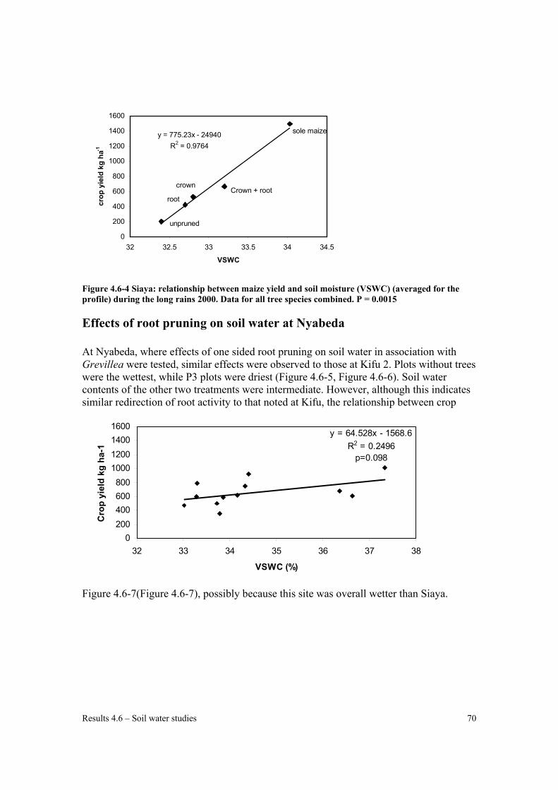
Results 4.6 – Soil water studies 70
y = 775.23x - 24940R2 = 0.9764
0
200
400
600
800
1000
1200
1400
1600
32 32.5 33 33.5 34 34.5
VSWC
crop
yie
ld k
g ha
-1
sole maize
Crown + rootcrown
root
unpruned
Figure 4.6-4 Siaya: relationship between maize yield and soil moisture (VSWC) (averaged for the profile) during the long rains 2000. Data for all tree species combined. P = 0.0015
Effects of root pruning on soil water at Nyabeda At Nyabeda, where effects of one sided root pruning on soil water in association with Grevillea were tested, similar effects were observed to those at Kifu 2. Plots without trees were the wettest, while P3 plots were driest (Figure 4.6-5, Figure 4.6-6). Soil water contents of the other two treatments were intermediate. However, although this indicates similar redirection of root activity to that noted at Kifu, the relationship between crop
y = 64.528x - 1568.6R2 = 0.2496
p=0.098
0200400600800
1000120014001600
32 33 34 35 36 37 38
VSWC (%)
Cro
p yi
eld
kg h
a-1
Figure 4.6-7(Figure 4.6-7), possibly because this site was overall wetter than Siaya.

Results 4.6 – Soil water studies 71
Figure 4.6-5 Effects of soil depth and tree root pruning on percent volumetric soil water content (%) pooled for all distances ( 0 – 7.8 m) from Grevillea tree line during the short rain 1999, long rain 2000 and short rain 2000 at Nyabeda, western Kenya. SED1 = Standard error of the means between depths in a treatment. SED2 = Standard error of the means between treatments for a given depth of soil profile.
1st season SR 1999
20406080
100120140160180200
20 25 30 35 40 45
SED1 = 0.78SED2 = 0.85
2nd season LR 2000
20406080
100120140160180200
20 25 30 35 40 45
One side rootprunedThe other sideun-prunedBoth sides un-pruned controlSole maize
SED1 = 0.13SED2 015
3rd season SR 2000
20406080
100120140160180200
20 25 30 35 40 45
SED1 = 0.16SED2 = 0.18

Results 4.6 – Soil water studies 72
30
31
32
33
34
35
36
37
38
39
Janu
ary
Februa
ryMarc
hMay
June Ju
ly
Augus
t
Septem
ber
Octobe
r
Novem
ber
Decem
ber
Janu
ary
Months
%V
SW
C
One-side root pruned The other side un-pruned Both sides un-pruned control Sole maize
Figure 4.6-6 Mean trends of % VSWC pooled for all soil depths and distances from the tree line over threee cropping seasons at Nyabeda, western Kenya
y = 64.528x - 1568.6R2 = 0.2496
p=0.098
0
200
400
600800
1000
1200
1400
1600
32 33 34 35 36 37 38
VSWC (%)
Cro
p yi
eld
kg h
a-1
Figure 4.6-7 Relationship between crop yield and soil moisture at Nyabeda, Kenya, during the short rains 99, long rains 2000 and short rains 2000

Results 4.6 – Soil water studies 73
Effects of root pruning on soil water at Kifu 2 Soil water was assessed, by neutron probe, at Kifu 2 in parallel with the crop studies. This report will focus on the April – July 2000 growing season, six months after the 2nd root pruning. Crop data for this season are provided in Table 4.4-3. Examination of the soil water data will concentrate on the 30 – 60 cm soil depths, where losses by evaporation are minimised and where tree and crop root distributions overlap and are in competition. Generally, soil was driest close to trees, and there was more soil moisture on the pruned side. Species effects were observed in April, June and July. Effects of ‘side’ and ‘pruning’ were similar to those observed on crops, with sub-sub plots which had been root pruned, showing significant effects in all months except June, whereas tree sub-plots which had been root pruned on one side, rarely showed effects. Effects of pruning on soil moisture at different depths are illustrated in Figure 4.6-8 and Figure 4.6-9. Highest values occurred in the pruned sub-sub plots and lowest on the opposite side of the row of the same trees. There was considerable variation in water use between the different plots: the crop only control used least, while Casuarina and Markhamia used most (Figure 4.6-10).

Results 4.6 – Soil water studies 74
Figure 4.6-8 Effects of pruning on sub-sub plot soil moisture in the 30-60 cm depth at 4.8 m distance from the tree in the April-July 2000 growing season.
Figure 4.6-9 Soil moisture content on the sub-sub plots at 30 – 60 cm depths, 4.8 m from the tree row during April to July 2000. Error bar represents SED
(a) April
0
20
40
60
80
25 30 35 40
Percent soil moisture
Soil
dept
h (c
m)
(b) May
0
20
40
60
80
25 30 35 40
Percent soil moisture
Soil
dept
h (c
m)
(c) June
0
20
40
60
80
25 30 35 40
Percent soil moisture
Soil
dept
h (c
m)
P3
P1
P2
(d) July
0
20
40
60
80
25 30 35 40
Percent soil moisture
Soil
dept
h (c
m)
252729313335373941
April May June July
Perc
ent s
oil m
oist
ure
P3P1P2

Results 4.6 – Soil water studies 75
Second phase – improved understanding of root pruning effects on soil moisture profiles These studies were conducted at a more widely spaced trial at Nyabeda2, and focussed on the two largest species on the site, Eucalyptus and Grevillea. New profile probes (Delta T Devices) were purchased for this study. Unfortunately, we encountered problems with these; many of the probes rapidly developed a fault so that readings at the maximum depth (1 m) were unobtainable. Furthermore, when probes were attached to the data logger, many readings were erratic and some were impossible (for instance, many of the probes indicated a diurnal variation in soil water at 1 m depth). Initial testing of the probes in the laboratory did not reveal these problems, which only became apparent when the equipment was installed in the field, where it was very difficult to track down the faults. We had extensive consultations with the manufacturer, who eventually shipped out some replacement probes (in March 03). The problem with unobtainable readings at 1.00m was tracked down to a cabling problem, while the problems with data logging appeared to have many causes. Despite many efforts with changing loggers and rewiring, the problems were never completely resolved. Because of these difficulties, the dynamic study of water movement in the profile was not possible, and the soil water data presented here are only from hand-held profile probe readings.
Figure 4.6-10 Soil water use by different tree species (difference in the % soil moisture between the wettest and driest months, during the April – July cropping season. Error bar represents SED.
0
2
4
6
8
10
12
Casuarina Grevillea Maesopsis Alnus Markhamia Control
Perc
ent w
ater
use

Results 4.6 – Soil water studies 76
Tree root dimensions in the root pruning zone Root pruning was first done in April 2002, before the first crop was sown, and was repeated in October 2002, before sowing of the second crop. Numbers of roots and their dimensions were recorded on each occasion (Table 4.6-1). Table 4.6-1 Number and cross-sectional area of roots in 15m long x 0.3 m deep root pruning trench at time of first root pruning (April 2002), and at repruning in October 2002 at Nyabeda 2, western Kenya (mean of 2 plots)
No. roots in 15 m of trench
No. roots > 1 cm diameter
Cross sectional area (cm2) of cut roots > 1 cm diameter
First root pruning April 02
Grevillea 248 129 1455 Eucalyptus 329 162 2230 Repeat root pruning October 02
No. roots in 15 m of trench
No. roots > 1 cm diameter
Cross sectional area (cm2)of all cut roots
Grevillea with crop 41 7 13 Grevillea without crop
42 4 7
Eucalyptus with crop 30 1 4 Eucalyptus without crop
32 0 5
Before first root pruning, both species had a considerable cross-sectional area of root in the top 30 cm of soil. The area of Eucalyptus root was 60 % greater than that of Grevillea. Six months later, root numbers had recovered to a certain extent, but roots were of small diameter and their total cross sectional area was negligible. There were indications that regrowth of Eucalyptus was proceeding more slowly than that of Grevillea, both in terms of root numbers and size. Root parameters were not measured on the untrenched plots, because of the risks of causing root damage.
Soil water and crop yield With Eucalyptus, on plots which were not cropped, soil water was consistently greater on the root pruned side, particularly at 3 m from the tree, indicating that less water was being extracted by the tree, and lower on the unpruned side (Figure 4.6-11). In the cropped plot, soil moisture was similar on both pruned and unpruned sides.

Results 4.6 – Soil water studies 77
Figure 4.6-11 Mean volumetric soil water content (m3m-3) in the top 0.5 m of the soil profile. Sequential readings in the same access tubes from August 02 to February 03.Trees are planted at 0 on the x axis and root pruning is at + 0.5 m from the tree (indicated by vertical line). Plots are with (upper) or without (lower) crops.
Crop yields were consistently higher on the root pruned side of Eucalyptus trees compared with the unpruned side (data not shown). Nevertheless there was still a strong gradient of declining crop yield towards the tree. The improved soil water status on the pruned side of uncropped plots represents the situation where tree root activity has been restricted, and there is no other vegetation to exploit the soil water which is available. By contrast where root pruned plots are cropped,
Eucalyptus cropped
0.00
0.02
0.04
0.06
0.08
0.10
0.12
0.14
0.16
0.18
-6 -4 -2 0 2 4 6
DIstance (m) from tree row
VSW
C m
3m3
08-Aug-02
09-Oct-02
19-Nov-02
25-Nov-02
13-Dec-02
20-Dec-02
03-Jan-03
17-Jan-03
12-Feb-03
22-Feb-03
Eucalyptus uncropped
0
0.02
0.04
0.06
0.08
0.1
0.12
0.14
0.16
0.18
-6 -4 -2 0 2 4 6
Di st a nc e ( m) f r om t r e e r ow
8-Aug-02
9-Oct-02
19-Nov-02
25th Nov
13-Dec-02
20-Dec-02
3-Jan-03
17th Jan 2003
12-Feb-03
20-Feb-03

Results 4.6 – Soil water studies 78
the water which has become available through restriction of tree root activity, has been largely utilised by the crop plants.

Results 4.8 – Pruning effects on crop yields in on-farm studies 79
4.7 Output 5. Tree root function After the Machakos site was no longer available, sapflow studies were conducted at Kifu, Siaya and Nyabeda. Studies at Kifu focussed on changes in sapflow immediately after root pruning, whereas studies at the Kenyan sites were conducted some time after pruning was done. At Kifu, when lateral roots on one side of Grevillea trees were cut, there was a significant reduction (p < 0.001) in sap flow through the trunk, but five days later, sap flow had recovered to the original levels Figure 4.7-1.
Figure 4.7-1 Effects of root pruning on mean daily sap flow in stems of Grevillea robusta at Kifu. Data are sapflow in stems of pruned trees divided by sap flow in stems of unpruned trees. On pruned trees, half of the lateral roots within 30 cm of the soil surface were cut on day 3.
However, not all species responded in the same manner: Maesopsis eminii at the same site showed no significant change in sap flow (Figure 4.7-2). In the prevailing environmental conditions at Kifu, it was not the unsevered lateral roots which compensated for the reduction in water absorbing area after root pruning, because sap flow through the remaining lateral roots did not change (Figure 4.7-3). Consequently, it seems that roots which were located more deeply increased their rates of sap flow to satisfy transpirational demand from the atmosphere. However, while that may have been the case at the time that this sap flow study was conducted, evidence from the crop yield studies (Table 4.4-6,Table 4.4-7) and soil water studies (Figure 4.6-9) indicates that there was redirection of activity to remaining lateral roots at other times of year.

Results 4.8 – Pruning effects on crop yields in on-farm studies 80
Figure 4.7-2 Effects of root pruning on mean daily sap flow in the stems of Maesopsis eminii trees at Kifu. Data are sap flow in stems of root pruned trees divided by the sap flow in stems of unpruned trees. On pruned trees, half of the lateral roots within 30 cm of the soil surface were pruned close to the root collar on day 3.
Figure 4.7-3 Sap flow through intact lateral roots of four tree species at Kifu, as a percentage of sap flow in the stem before and after severing about 50 % of the lateral roots.

Results 4.8 – Pruning effects on crop yields in on-farm studies 81
4.8 Output 6. On farm experimentation
4.8.1 Uganda – pruning effects on crop yields (Kabale) (Experimental protocol no. 1)
First season after pruning In this season, yields of beans were compared in crown, crown and root and unpruned plots. Measurements were taken on the 10 rows of crop nearest the tree and significant effects of pruning on yield occurred at each distance (Table 4.8-1). There was no significant difference between tree species. Over the whole cropping area, yield with combined crown and root pruning was 344% greater than that of the unpruned plots, while crown pruning alone doubled crop yield. Both pruning treatments affected yield across the whole plot, but the effect of combined pruning was stronger than crown only as distance increased. Table 4.8-1 Effects of pruning on bean yield (kg ha-1): first season after pruning, at different distances from tree rows
crown crown and root no prune 0 - 1 m 232.7a* 253.7a 87.3b1 - 2 m 279.7a 403.7a 97.0b2 - 3 m 381.0b 577.7a 149.7c3 - 4 m 233.3b 510.0a 123.3c4 - 5 m 250.0b 463.3a 183.3cmean 275.3b 441.7a 128.1c * values followed by different letters are significantly different within a particular distance from the tree row Although pruning had an effect all the way across the plot (Figure 4.8-1), a peak effect was apparent with both pruning treatments at 2 – 3 m from the tree row.
0.0
100.0
200.0
300.0
400.0
500.0
600.0
700.0
0 - 1 m 1 - 2 m 2 - 3 m 3 - 4 m 4 - 5 m
crow n
crow n and root
no prune
Figure 4.8-1 Effects of pruning treatment on crop yield (kg ha-1)at different distances from tree row

Results 4.8 – Pruning effects on crop yields in on-farm studies 82
Second season after pruning The following season, root pruning was repeated before the crop (maize) was planted. Crop yields were measured over a greater distance than the preceding season, and a ‘no tree’ plot was included. Species x treatment interactions were present up to 7.5 m away from the tree line (Table 4.8-2; Figure 4.8-2). There were very wide error bars on the data. Alnus was the more competitive species, for this species, combined crown and root pruning was more effective in controlling competition than only crown pruning. Grevillea was less competitive, and combined crown and root pruning was no more effective than crown pruning on its own. With no tree, yields were comparatively high at the lower side of the terrace where trees were normally present. However, at the upper side of the terrace, yields tended to be higher on plots with pruned trees than in the other treatments. Table 4.8-2 Effects of pruning on maize yield (kg ha-1) at different distances from the tree row, second season after main pruning, root pruning repeated before this season
Alnus Grevillea crown crown & root no prune crown crown & root no prune no tree p 0 - 1.5 m 904ab* 1277a 513b 988ab 1173a 1006ab 1462a 0.051.5 - 3 m 1057ab 1224a 653b 1346a 1513a 991ab 1571a 0.013 - 4.5 m 1044bcd 1535ab 762d 1622a 1580a 902cd 1313abc 0.0044.5 - 6.0 m 1173b 1984a 1182b 1480ab 1220b 986b 1842a 0.0026 - 7.5 m 1011c 1682a 940c 1575ab 1264bc 1177bc 1286abc 0.006 Mean 0 – 4.5 m 1002ab 1345a 643b 1319a 1422a 939ab 1449a <0.001Mean 0 - 7.5m 1038bc 1492a 806c 1403a 1350ab 996c 1497a <0.001* values followed by different letters are significantly different within a particular distance from the tree row Figure 4.8-2 Effects of pruning on maize yield (kg ha-1) at different distances from the tree row, second season after main pruning, root pruning repeated before this season

Results 4.8 – Pruning effects on crop yields in on-farm studies 83
Third season after pruning In the subsequent beans season, yields were generally low and the benefits of pruning were diminishing as trees regrew. Overall, Alnus was more competitive than Grevillea. Pruning effects were not significant at several of the distances from the trees, nevertheless, at the plot level, a significant reduction in crop growth by unpruned Alnus was apparent. Pruning treatments were effective in reducing the competition by Alnus, but there was no difference between them (Table 4.8-3). The effects were less clearcut with Grevillea, however, yields on plots with crown-pruned trees were still significantly higher than with unpruned trees. Yields on unpruned Alnus plots were significantly lower than plots without trees. Table 4.8-3 Effects of pruning on bean yield (kg ha-1) at different distances from the tree row, third season after main pruning
Alnus Grevillea No tree crown crown & root unpruned crown crown & root unpruned p 0 - 1 m 101.7b 111.3ab 20.3c 189.3a 160.3ab 14.7c 87.7bc 0.0011 - 2 m 115.7 162.3 19.7 169.0 114.3 140.3 156.0 ns2 - 3 m 236.3ab 254.7ab 64.3c 355.3a 223.7ab 167.7bc 307.0ab 0.0093 - 4 m 215.3 233.3 116.7 337.7 260.7 196.7 254.3 ns4 - 5 m 230.0 275.7 189.3 314.0 299.7 264.7 250.3 ns5 - 6 m 246.3 211.7 229.0 332.7 409.0 236.3 276.0 ns6 - 7m 355.7 243.3 257.0 300.0 334.7 202.3 289.0 ns7 - 8 m 446.7a 353.0ab 277.0ab 372.3ab 446.0ab 256.0b 315.0ab 0.015 rows 0 - 5m
180.0abc 207.3ab 82.0c 273.3a 203.3ab 156.7bc 249.3ab 0.007
rows 0 - 8 m 243.3ab 230.8abc 146.7c 296.3a 275.8a 185.0bc 242.1ab 0.035
0.0
500.0
1000.0
1500.0
2000.0
2500.0
0 - 1.5m
1.5 - 3m
3 - 4.5m
4.5 -6.0 m
6 - 7.5m
7.5 - 9m
9 -10.5 m
Alnus crownAlnus crown and rootAlnus no pruneGrev crownGrev crown and rootGrev no pruneno tree

Results 4.8 – Pruning effects on crop yields in on-farm studies 84
Figure 4.8-3 Effects of pruning on bean yield (kg ha-1) at different distances from the tree row, third season after main pruning
0
50
100
150
200
250
300
350
400
450
500
0 - 1 m 1 - 2 m 2 - 3 m 3 - 4 m 4 - 5 m 5 - 6 m 6 - 7m 7 - 8 m
Alnus crownAlnus crown and rootAlnus no pruneGrev crownGrev crown and rootGrev no pruneno tree

Results 4.8 – Pruning effects on crop yields in on-farm studies 85
Discussion It should be noted that in this study, there was no trenching between the experimental plots and therefore tree roots will have spread between plots. At the same time, there will have been shading between plots. Both these factors will have contributed to the high variability of some of the data, and will probably have minimised the apparent effects of pruning. Figure 4.8-4 Summary of crop yield in the different cropping seasons: yield (kg ha-1) at 0 – 5 m from trees (beans) and 0- 4.5 m from trees (maize) after different pruning treatments in comparison with no tree control
Table 4.8-4 (a) Ratio of crop yield in the pruning treatments to the respective unpruned control and (b) ratio of crop yield in the combined crown and root pruning treatment to yield when the trees were only root pruned
Alnus Grevillea a. Crown Crown & root Crown Crown & root Beans1 0 – 5m 2.5 4.8 2.1 3.0 Maize 0 – 4.5m 1.6 2.1 1.4 1.5 Beans2 0 – 5m 2.2 2.5 1.7 1.3 b. c&r:r c&r:r Beans1 0 – 5m 1.9 1.4 Maize 0 – 4.5m 1.3 1.1 Beans2 0 – 5m 1.2 0.7
Effects of the pruning treatments followed similar patterns in all three cropping seasons (Figure 4.8-4). Combined crown and root pruning was more effective in
0.0
50.0
100.0
150.0
200.0
250.0
300.0
350.0
400.0
450.0
500.0
crown crownandroot
noprune
crown crownandroot
noprune
Alnus Grev No
Bea
ns k
g ha
0.0
200.0
400.0
600.0
800.0
1000.0
1200.0
1400.0
1600.0
Mai
ze k
g ha Beans 1
Beans 2Maize

Results 4.8 – Pruning effects on crop yields in on-farm studies 86
controlling competition than crown pruning alone. Unpruned Alnus tended to be more competitive than unpruned Grevillea. Alnus is an N fixer and might have expected to promote better crop growth than Grevillea after competition had been removed. However, although the improvement in yield relative to unpruned control was greater with Alnus (Table 4.8-4), the actual yields were no larger, indicating that the trees were not contributing to crop yield through N fixation. Another study in the locality (David and Raussen 2003) found that tree fallows on the lower part of the terrace did not increase soil nitrogen or crop yield, whereas on the poorer soil conditions on the upper terrace, some species did improve soil nitrogen and yield. In their study, Alnus acuminata did not improve soil N, and although it improved crop yield, other species, especially Calliandra and Sesbania, were more effective. Relative improvement in yield was greatest in the first cropping season after pruning, whereas the second and third seasons were similar to each other, despite the repetition of root pruning before the second season. Average crop yields were very low. The average yield of beans in the second season on the no tree plots was about 0.25 tonnes ha-1, while maize yield on no tree plots was about 1.5 tonnes ha-1. For Kabale District, the average yield of beans is 0.75 tonnes ha-1 and for maize is maize is 1.2 tonnes ha-1, well below the potential yield of 4 tonnes ha-1 (NEMA 1996). However, the limitations of the plots in this study should be noted, particularly the lack of trenching between them. In Kabale, like much of Uganda, increasing agricultural production appears to have been achieved by increasing the area of land under production (Carswell 2002) rather than increasing yields per plot. Growing trees and crops together enables exploitation of unused niches within existing fields, and David and Raussen (2003) have shown the potential for tree planting on the upper slope of terraces. The tree management techniques described here clearly reduce competition and enable the farmers to balance their requirements for wood and crop production through manipulation of the trees. Furthermore, increasing tree cover will protect slopes and contribute to C sequestration. If tree planting on terraces is to be encouraged as part of the local land management system, the trees must be managed if crop yields are not to be compromised. By 7 years after tree planting , maize and bean crop yields on the unpruned plots were approximately half those on the no tree plots. Tree pruning enables farmers to substantially regain crop yield, and at the same time obtain useful products from the trees (fuel and stakes). Although tree growth is reduced (Table 4.3-5), management by pruning appears to offer a good compromise between the production of short and long term components of the cropping system. The frequency of repruning will be determined by the costs and benefits. Effects of pruning were strongest for the first cropping season after pruning and were smaller, but similar during the next two seasons, during which regrowth of roots and crowns was occurring. Combined crown and root pruning was more effective for Alnus than Grevillea, and it may be less cost effective to do root pruning on the latter species (although it takes very little time). First crown pruning of the trees took an average of 20 minutes per tree, and root pruning took 10 minutes. Repeat crown and root pruning took less time because there is less material, of smaller diameter, to cut (the second crown pruning

Results 4.8 – Pruning effects on crop yields in on-farm studies 87
took 10 minutes per tree). Root pruning could easily be repeated at cultivation time each season. These trials have indicated the way forward for farmers in the Kabale area and they are now adapting these methods to suit their individual purposes.
4.8.2 Uptake of pruning Surveys were conducted at the end of the project at Kabale and Siaya where studies continued throughout the project. These indicated contrasting attitudes to pruning. While farmers at both locations had seen that pruning could improve crop yields, few farmers at Siaya showed any sign of putting the work into practice, while adoption was evident with Kabale farmers. Because there were many differences between approaches at the two sites, it is not possible to disentangle the reasons for the difference in adoption, however it is worth noting that studies at Kabale were conducted on farm, the local partners had excellent links with the local community and the trees in the study were relatively small. By contrast, at Siaya, studies were not on farm (although local farmers were involved in management) the trees were much bigger and therefore more difficult to prune and there was less of a project presence in the area as the local HQ was some distance away.

Results 4.8 – Pruning effects on crop yields in on-farm studies 88
4.8.3 On-farm experimentation in Kenya – pruning effects on crop yield at Kibwezi (Experimental protocol no. 7)
Location Effects of pruning were examined in on-farm studies at Kibwezi in eastern Kenya. This location usually receives bimodal rainfall averaging 500 mm annually although there are great variations within seasons. The altitude at trial site is 850 - 900 m asl. The soils are well drained and sandy. Melia volkensii was selected as the target tree species, and studies encompassed seven farms.
Plant material Crop yields were evaluated around isolated trees (at least 30 m from adjoining trees), where other influences were minimized. A total of 27 trees of mixed ages and sizes were included in the study. Pruning treatments were randomly allocated to individual trees. The diameter ranges of the trees in each treatment were as follows; control (trees un-pruned) (13.1-34.9 cm), crown pruning (17.4- 43.5 cm), crown & root pruning (21.2 – 29.2 cm) and root pruning (17.3 – 37.0 cm). Experimental details Maize seed (DH1 variety) was supplied to the farmers to establish maize intercrop around the selected trees. Thereafter, each of the selected trees was subjected to one of the four pruning treatments:
• P1 = Severe crown pruning 90-95% (Cr); • P2 = Root pruning (Rt); • P3= Severe crown pruning + Root pruning (Cr+Rt) and • P4 = Control (Co), (neither crown nor root pruning were done).
The pruning operations were done before the rains. For the crown, the branches spread and crown sizes were determined on each standing tree. 90 - 95% of the crown (side branches) was then subjectively removed using a panga but the top of the tree was not lopped. The root pruning was done either as an arc or as a line trench on one side of the tree where crop growth along a transect could be assessed. The trench was dug using a jembe and panga to cut off roots within 30 cm depth at 50cm from the tree trunk. In both types of root pruning, roots were severed from an arc of approximately 180. Once pruned, roots were removed and the trench was refilled before maize planting. After pruning treatments were applied, the maize crop was planted at spacing of 100cm * 30cm up to 15m from the tree trunk. Assessment/Measurements

Results 4.8 – Pruning effects on crop yields in on-farm studies 89
Tree diameter at breast height (DBH) was taken at every rain season during pruning operations. Biomass of the removed branches was measured for dry matter production. Crop growth and yields were measured along the transect away from the tree bole at distance intervals of 2m starting at 1m from the tree. At each sampling distance, the five nearest maize plants were assessed. Results Plots which were crown pruned, or crown & root pruned had significantly higher crop yields than control (unpruned) or root pruned plots. Only control plots showed a treatment x distance interaction (p=0.046). Regression lines of yield vs distance were parallel for Cr, Rt and Cr+Rt treatments, indicating that the effect of distance from the tree on maize crop yield was similar for these treatments (Figure 4.8-5). Combined crown and root pruning had the highest intercept, indicating that competition from the tree was least in this treatment.
Figure 4.8-5 Regression of maize crop yield against distance from Melia volkensii trees for the different experimental treatments. (green = unpruned control), red = crown pruned, dark blue = root pruned, sky blue = crown and root pruned).
No effects of pruning on tree growth rate were observed during the period of this study. These assessments, and further evaluations of effects of pruning on crop yield at this site are being continued by KEFRI.


Results 4.9 – HyPAR modelling 91
4.9 Report on HyPAR modelling Deena C. Mobbs, Centre for Ecology & Hydrology HyPAR was tested by running with ‘bare soil’, ‘crop only’, ‘tree only’ and ‘agroforestry’ options. At each stage the results were compared with field data from Siaya. Standard maize parameters were used for the crop and Grevillea parameters for the trees at this site. The tree growth parameters were calibrated with Siaya data (dbh, height). Crown pruning was available as an option in the model. Various approaches were explored to add new management options relating to root pruning and more extensive crown pruning, but (because of the structure of the model) these proved to be very difficult. Extensive model methodology changes and recoding would have been required to properly implement the changes. Patterns of tree and crop growth were examined with unpruned and pruned trees over a simulated period of 15 years. Soil water and nutrient content data were recorded but not compared with field data. Output from the model included crop yield data, tree dimension and carbon content data for pruned and unpruned trees. These can be used to derive financial equivalents.
4.9.1 Summary HyPAR is an agroforestry model created by combining two models such that the tree-specific routines from Hybrid are used to grow trees with an understorey of crop based on routines from PARCH. Biophysical models of agroforestry such as HyPAR describe competition in time and space for light, water and nutrients and can be used to estimate the crop yield in a range of soil, weather, management and tree/crop combinations. Year to year comparisons of yield give an indication of the risk to a farmer and the likely long-term productivity decline due to soil impoverishment or climate change. This type of model can predict economic outputs in terms of grain yield, crop residue, timber volume and tree-fodder. The intention is to use HyPAR to generate long-term yield predictions using different tree density and crop combinations with management methods including crown and/or root pruning. Outputs that can be used directly for financial estimates such as long-term wood and grain yields, fodder and risks of failure would then be integrated with non-biophysical data (e.g. income requirements, labour availability and costs, food requirements, food-security preferences, land availability etc.) to predict the multiple costs and benefits arising from a range of agroforestry management options. The project is based in two countries, Kenya and Uganda, with a total of eight field sites. The Kenyan site at Siaya was chosen as the primary site in this exercise because the available data were more complete for climate, soil, tree and crop at the time the modelling was carried out. After preparing the climate input, the soil profile, initial conditions and selecting appropriate hydrology routines HyPAR was used to model tree and crop growth for Siaya. First, trees were grown on their own, then sole crop and finally the full agroforestry simulation of crops and trees growing simultaneously. Simulations with trees were carried out with and without management options applied. Trees: The tree species chosen was Grevillea and four trees were planted in a field of 7m by 8m to simulate typical conditions at Siaya with an initial ‘diameter at breast height’ (dbh) of 1.5cm. The trees were grown for 15 years with and without management, the runs being repeated 10 times with random daily climate variation. All results presented are average values for the 10 replicate runs. HyPAR allows two alternative light interception routines, known as ‘uniform’ or ‘disaggregated’. In uniform mode, the trees are assumed to be randomly placed within the field, their canopies cast a uniform shadow across the whole field and the roots are

Results 4.9 – HyPAR modelling 92
assumed to extend throughout the field with a uniform distribution horizontally and a declining vertical distribution. In disaggregated mode the field is divided into a number of square plots and trees are placed in a specific plot. The individual tree canopies are assumed to be elliptical and the roots extend away from the tree with exponentially declining density as well as the vertical decline with depth. While the same light absorption method is used to calculate tree assimilation in each mode, the tree growth will differ due to varying availability of water and nutrients in the soil cells. In uniform mode, all trees in the field will grow at the same rate when starting from the same initial size as they experience an identical environment. The trees reach a height of approximately 19m with a crown height of approximately 12m (i.e. height to base of crown is 7m) and dbh of 22cm. Most of the biomass carbon is held in sapwood. In disaggregated mode, HyPAR was used to grow four evenly spaced trees and tree growth is the same as in previous simulations for the first 5 to 6 years but then diverges with the ‘uniform’ tree growing a larger trunk and a more compact crown. Analysis of the results show that the C:N ratio for the tree compartments is much higher in the ‘disaggregated’ tree suggesting that the tree was unable to take up sufficient nitrogen compared with a ‘uniform’ tree. Crop: For Siaya, the crop chosen is maize. Maize plants were planted at a density of 40000 per hectare in a field of 7m by 8m to simulate typical conditions at Siaya. Two crops are grown per year with earliest planting dates set at Julian day 63 (3rd March) and 239 (26th August). The exact planting dates for each run are dictated by soil water conditions, planting will not occur unless the top 40cm of soil contains at least 22mm of water. The crop seasons were simulated for 15 years, the runs being repeated 10 times with a different seed to generate a random variation for the climate. The early crop generally has a higher yield (mean 0.75 t/ha) than the late season crop (mean 0.51 t/ha) The late season crop generally takes up more resources from the soil over the course of the growing season than the early crop but the conditions are not suitable to turn this into grain. Agroforestry: Both tree and crop grow well individually when driven by the simulated Siaya climate data. HyPAR is used to grow both tree and crop in the same field to simulate a simple agroforestry experiment – the plants compete for water and nutrient in the soil and the trees shade the crop. In uniform mode the trees are assumed to be spread randomly in the field and their roots and crowns extend evenly across the whole area. Thus all crop plants are affected equally by the presence of the tree overstorey. Unmanaged trees grow rapidly so that after just 5 years the crop is unable to grow under the intense competition. The amount of water taken up by young trees is an order of magnitude less than that taken by the crop and the trees extract their water from lower in the soil profile, especially towards the end of the year after the rains. Similarly, the amount of nitrogen taken up by young trees is small compared with the crop but the presence of the crop roots forces the tree to extract N from the lowest soil layer in the late season when N is in short supply. Older trees extract more resources to the exclusion of crop. In disaggregated mode, the crop yields for three rows of crop are combined and averaged over 10 runs to give an average figure for yield relative to distance from a tree. Close to the tree the crop yield declines rapidly from 0.4t/ha to zero after 5 years. At a distance of 10m from the tree, the crop continues to yield grain for approximately 13 years although the amount is small. Further from the tree (outside the range of the tree roots) the yield does not decline with time. The total for the whole field indicates

Results 4.9 – HyPAR modelling 93
that although the crop cannot grow under the tree, the farmer would obtain some crop product from this area of land. Management Options: Initially, four management schemes were defined: ‘crown pruning’ with either 50% or 90% of the crown removed every two years starting in year 5 on a day just prior to when the first crop would be planted, ‘pollarding and pruning’ by removing the top part of the crown down to 4m height followed by pruning 90% of the foliage from the base up every two years starting in year 5 on a day just prior to when the crop would be planted, and ‘root pruning’ to 30cm depth every year from year 5 on a day before the crop season. Crown pruning is carried out in the model by removing the lower portion of the canopy foliage and an appropriate fraction of the wood biomass to represent lost branches on the specified day. When foliage is removed, the root biomass is automatically reduced by the model because there is an assumption that the two values are in a user-defined fixed ratio. Investigation of the HyPAR code revealed that pollarding cannot be correctly modelled in the current version. If the height of the tree is truncated while leaving the stem dbh unaltered, the daily carbon allocation subroutine immediately recalculates the height from dbh thereby ‘growing’ the tree back to its original height on the same day as the pollarding took place. This cannot be changed without major changes to the methodology in the model. Similarly, root pruning proved very difficult to implement dynamically. Each model day, the foliage growth is estimated based on photosynthesis rates, subsequent growth gains and expected litter fall losses, the fine root biomass is set based on a user-defined parameter that gives the ratio between foliage and root biomass, and finally this biomass is distributed in the soil layers depending on the user-defined half-depth parameter (disaggregated mode also has a ‘half-width’ parameter). As with pollarding, if the roots are removed the growth routines immediately ‘regrow’ them back to the expected values cancelling out the pruning action. Different methods were examined to implement dynamic root growth but each would require extensive code and model design modification. There was insufficient time to achieve this in this project and as HyPAR is no longer being developed elsewhere, extensive code modifications was not appropriate. Tree management simulations were therefore limited to crown pruning for uniform mode. In disaggregated mode, the tree parameter set includes four extra values controlling root distribution. The maximum range away from the tree reached by the roots is a function of a parameter and the current tree height. A simple method to model root pruning is to change the parameter to a smaller value thus restricting root expansion to mimic regular manual cutting. Tree crown pruning in HyPAR, with these soil and climate conditions, has little effect on the overall height of the tree, the trees reach a height of approximately 19m with a dbh of 22cm. However, the pruning events alter the distribution of carbon and relative sizes of the tree compartments compared with the unmanaged simulations. The trees have more heartwood and less sapwood, the difference increasing with pruning intensity. The trees are first crown-pruned in the 5th year, and again in years 7, 9, 11 and 13. By this time, the trees have grown so large that crown pruning has little effect on crop yield in these simulations although there is some grain yield return in time following the 90% pruning events. In disaggregated mode, crown pruning increases the total (per field) yield in the later years by increasing the yield closer to the tree although yield away from the tree may be reduced. To examine the effects of root pruning, simulations were carried out in which the tree root horizontal distribution width parameter was reduced to 0.1. This means that the

Results 4.9 – HyPAR modelling 94
tree roots were restricted to a radius of 0.1 times the tree height. Crop growth increases further than 1m away from the tree but this is not entirely due to the absence of tree roots – with restricted root growth the tree grows more slowly and reaches only 17m in height with a crown of radius of just 3.7m. With restricted roots and 90% crown pruning applied, the effects of the tree on the crop is reduced. Rainfall: In order to simulate the possible impact of climate change at Siaya, and to explore the effect of management on agroforestry in drier locations, a set of simulations were carried out with the Siaya environment and reduced rainfall. Reduced rainfall for a given site can be achieved by decreasing the number of wet days per month (that the plants experience more days with no rain) or by reducing the rain per wet day (less intense rain events). The stress placed on the tree and crop growth will be different so the plants will respond in different ways. In the standard simulations the average sole crop yield is 0.63 t/ha and a 20% drop in rainfall by reducing the rain intensity leads to a corresponding drop in yield to 0.48 t/ha. However, a 20% reduction in rainfall created by reducing the rainfall frequency leads to a small increase in yield to 0.64 t/ha. This may be due to reduced evaporation from the soil, a different infiltration pattern into the soil or timing of the rainfall events relative to the crop season. When trees are added to the simulation (unmanaged or crown pruned at 50% and 90% as before) a similar pattern is seen – the reduced rainfall intensity leads to a 20% drop in yield whereas a reduced rainfall frequency increases crop yield by up to 45% compared with the sole crop simulations. Movement of water through the soil also influences nutrient availability making comparisons between sites very complex.

Results 4.9 – HyPAR modelling 95
4.9.2 Modelling tree-crop competition Managing dryland tree-crop competition for water is crucial for maintaining crop yield and agroforestry adoption. Studies under R7342 showed that tree - crop competition at sites in Kenya and Uganda with 1000 – 1400 mm annual rainfall could be substantially reduced by crown and root pruning, separately and in combination. Concentrating on combined crown and root pruning, this extension will broaden studies on tree survival and crop yield into drier marginal farmland in Kenya (650 mm rainfall), and will consolidate previous studies in the 1200 mm rainfall zone. Data will be used to improve HyPAR, develop an economic model able to assess the impact of pruning on farmers’ income, and determine the ‘envelope’ of suitability of this approach. Close collaboration with NGOs and CBOs will reveal barriers to adoption and demonstrate the development potential of the technology at various socio-economic conditions and spatial scales.
4.9.2.1 HyPAR HyPAR (Mobbs et al. 1998) is an agroforestry model created by combining the models Hybrid (Friend et al. 1997) and PARCH (Bradley and Crout 1996). The tree routines from Hybrid are used to grow trees from saplings with an understorey of crop based on routines from PARCH with crop development regulated by thermal time and drought stress. HyPAR v1.0 was driven by daily climate, either historical or computer-generated, calculated light interception and water use by a horizontally-uniform tree canopy (which was always above the crop), annual tree biomass increment (net primary productivity), the light and water available to an understorey crop and hence crop growth and potential annual grain yield. It included the soil water movement and uptake routines of PARCH, and utilised those parts of Hybrid which determine light interception, water use, tree productivity and biomass partitioning. Leaf-shedding or tree death can occur in response to sustained negative net photosynthesis or water stress. Hybrid v1.0 was used by Cannell et al (1998) to predict the 50-year mean 'potential' sorghum yields and overstorey net primary productivity in nine climates (348mm - 2643mm rainfall) with uniform overstorey leaf area indices of 0 to 1.5. They concluded that simultaneous agroforestry may enable more light and water to be 'captured' than sole cropping. However, in regions with less than 800 mm rainfall it is difficult to increase total productivity without jeopardising food security because of low water use efficiency of trees and sensitivity of crops to shading. The authors recognised that conclusions from this early version of HyPAR ignored the soil fertility relations of trees, their potential access to deep water-tables, and other economic benefits such as shade, fuel and fodder. Tree management such as pruning was not possible in this early version of the model. HyPAR v2.0 introduced competition for nitrogen and was used by Lott et al (1998) to test predictions of maize growth in Kenya. Later versions included improved soil water routines and options for management of the tree canopy including simple crown pruning (from the base upwards) and tree thinning (reducing the number of trees growing in the modelled area). Biophysical models of agroforestry systems must pay particular attention to root architecture because tree roots have a capacity to absorb water and nutrients from great depths and horizontal distances. The current version of HyPAR (v3.0, see Figure 4.9-1) includes daily rather than annual allocation of tree photosynthate, routines to represent disaggregated (i.e. clumped) canopy light interception and competition for water and nutrients between the roots of trees and

Results 4.9 – HyPAR modelling 96
crops in a horizontal as well as vertical direction if used in ‘disaggregated mode’. Below-ground competition for water is simulated by describing vertical water movement, soil water status, crop root growth, crop and tree root distributions and water abstraction in up to 15 soil layers. However, the tree roots do not ‘grow’ from day to day in the model. On each simulation day the total fine root biomass is estimated to be directly proportional to leaf biomass and this root biomass is distributed in the soil according to the defined rules.
Figure 4.9-1 Illustration (not using strict system dynamics notation) of the main flows of carbon, water and nitrogen in HyPAR v3.0. Dashed lines represent influences on the crop assimilation processes. Solid lines are flows between compartments. Water contents and pools of different half-lives are calculated for up to 15 soil layers. Tree and crop management options, and horizontally disaggregated light interception and resource uptake are also provided.
Biophysical models of agroforestry such as HyPAR describe competition in time and space for light, water and nutrients, and can be used to estimate the crop yield in a large range of soil, weather, management and tree-species combinations. Year to year comparisons of yield give an indication of the risk to a farmer, and the likely long-term productivity decline due to soil impoverishment. This type of model can therefore predict economic outputs in terms of grain yield, crop residue, timber volume and tree-fodder, but they do not address other issues of importance to the farmer - such as input costs, labour requirements, or land-availability. The intention is to use HyPAR v3.x to generate long-term yield predictions using different tree density and crop combinations with management methods including crown and/or root pruning. Outputs that can be used directly for financial estimates such as long-term wood and grain yields, fodder and risks of failure would then be integrated with non-biophysical data (e.g. income requirements, labour availability

Results 4.9 – HyPAR modelling 97
and costs, food requirements, food-security preferences, land availability etc.) to predict the multiple costs and benefits arising from a range of agroforestry management options.
4.9.3 Project Sites The project is based in two countries, Kenya and Uganda, with seven locations used for field work (Table 4.9-1). Table 4.9-1 Field site location and description
Country Site name Rainfall 1 Kabale Bimodal 1000 – 1500
mm Uganda
2 Kifu Bimodal 1400 mm 3 Machakos Bimodal 650 mm 4 Kibwezi /
Kitui Bimodal 650 - 700 mm
5 Siaya Bimodal 1200 mm 6 Nyabeda 1 Bimodal 1600 mm
Kenya
7 Nyabeda 2 Bimodal 1600 mm
4.9.4 HyPAR Simulations
4.9.4.1 Climate Selection HyPAR requires input in the form of daily weather data including precipitation, solar radiation, maximum and minimum temperature. Thus before any simulations can be carried out we need to provide adequate climate data. Daily weather data can be supplied from meteorological records or by generating daily from monthly means using the built-in weather generating program (Richardson and Wright 1984, Geng et al. 1986). The generator is driven by mean monthly values for sunshine, precipitation and temperature. Monthly values are available for half-degree gridded ‘pixels’ globally, these data are more fully described by Friend (1998).
4.9.4.1.1 Siaya The Kenyan site at Siaya was chosen as the primary site because the available data were more complete for climate, soil, tree and crop. Figure 4.9-2 shows available rainfall data for the Siaya area. Data recorded at the site (grey bars) were measured over 3 years (Tefera 2003) and gave an annual total of 1120mm while the black bars show the long-term average measured over 28 years for the local region (862mm a-1). Rainfall data from the nearest half-degree pixel (00N 340E) taken from Friend’s database are shown by the open bars and give an annual total of 1126mm. The long-term and gridded data are based on averages over a large area, which includes the field site, while the recorded data are based on a short time period. For the simulations a mean monthly data set is required from which daily data can be generated for 15 years or more with an appropriate overall average for both monthly variation and annual total. An adjusted monthly mean data set was created and is shown in Figure 4.9-2.

Results 4.9 – HyPAR modelling 98
Figure 4.9-2: Monthly rainfall data for Siaya, showing data measured between April 1998 and July 2000, the long-term average (measured over 28 years for the region) and the monthly mean data for the pixel at 00N 340E.
Insufficient data were available to repeat this process for the other climate variables. Values for these were taken from the half-degree pixel 00N 340E, as shown in Table 4.9-2. For the simulation runs described below, results presented are mean values output from 10 simulations runs each with different generated climate. Mean monthly rainfall generated by the model is shown in Figure 4.9-3, total annual rainfall varied from 978mm to 1072mm, similar random daily, monthly and annual variation is generated for all climate variables.
0
50
100
150
200
Jan Feb Mar Apr May Jun Jul Aug Sep Oct Nov Dec
Month
Rainfallmm
Field data Long-term average Gridded data Adjusted

Results 4.9 – HyPAR modelling 99
Table 4.9-2: Mean monthly climate data used as input to the HyPAR simulations for Siaya.
Figure 4.9-3: Ten simulation runs of monthly rainfall generated by HyPAR, using the values in Table 4.9-2 as input. Daily variation is generated for each simulation day.
4.9.4.2 Soil Characteristics Having selected the climate data for a site, the second task (before running crop or tree simulations) is to select the soil environment as defined within HyPAR and the most suitable hydrology and pedotransfer function routines for that soil.
Month Fraction of wet days
Rain per wet day mm
Total Rainfall mm
Max. temp. oC
Min. temp. oC
Solar Radiation W/m2
Relative humidity
Jan 0.27 5.45 45.63 27.90 17.71 234.40 69.24 Feb 0.31 6.97 60.09 28.29 17.91 244.10 69.88 Mar 0.45 8.22 115.11 28.15 18.05 243.96 72.34 Apr 0.63 9.68 183.29 27.55 17.45 236.61 75.38 May 0.61 9.27 175.29 27.00 17.00 222.78 75.02 Jun 0.35 7.28 76.88 26.60 16.41 216.35 70.63 Jul 0.30 6.04 55.21 25.86 16.14 214.95 69.67 Aug 0.28 5.59 47.96 26.02 16.58 223.15 70.56 Sep 0.28 5.75 47.57 26.66 16.75 237.00 70.52 Oct 0.29 5.83 53.12 27.60 17.60 238.50 70.92 Nov 0.41 8.06 99.11 27.55 17.45 233.38 71.63 Dec 0.37 7.28 83.10 27.54 17.26 231.27 70.92
1042.36 mm a-1 22.3 oC annual mean 231.7 Wm-2
annual mean
71.4 annual mean
0
50
100
150
200
250
Jan Feb Mar Apr May Jun Jul Aug Sep Oct Nov Dec
Month
Total rainfall for month,
mm

Results 4.9 – HyPAR modelling 100
The soil profile in HyPAR is divided into a number of discrete layers (maximum 15), with narrower layers near the surface where changes are more dynamic, and wider layers at depth. Each soil layer may have a different soil type as defined by the sand, silt and clay content and the bulk density. If the disaggregated canopy option is selected, the field is also divided into a number of horizontal grids and the vertical soil profile within each grid is independent (nutrients and water flow vertically only) although tree roots may extend across the whole field. Individual crop plant roots are confined to one grid. For each model timestep, in addition to the physical properties of depth and soil type, a soil layer has the following dynamic properties: water content (mm, divided into amounts available or unavailable for plant uptake), mineral nitrogen content (mg/kg), fresh organic matter (C and N, kg/ha) divided into five pools with differing decomposition rates, humus (C and N, kg/ha) and root length per unit volume for a crop and, potentially, several trees (mm/mm3). Within each soil layer the processes of water movement, leaching, soil organic matter decomposition, mineralisation of organic nitrogen, the immobilisation of mineral nitrogen and uptake by plants are simulated as daily incremental transfers. HyPAR offers several hydrology and pedotransfer function options, making a total of 13 possible combinations. Some combinations are better suited for sandy soils while others were designed for clay soils (Arah and Hodnett 1997a). All options require information about total soil depth, number of layers and the sand, silt and clay composition of each layer together with initial water and nutrient content (fresh organic matter, humus and mineral nitrogen). Other information required by some options includes bulk density, crack depth, crusting and macropore distribution. To select the optimum hydrology and pedotransfer function routines at each site, and the optimum starting conditions, basic information for soil depth, layer structure and soil composition is obtained and used to drive the model for a 30-year run with ‘bare soil’ i.e. with no tree or crop growing. Over this time scale, the water content in each layer will reach an equilibrium depending on the soil composition and total rainfall. The equilibrium soil water content is compared with field measurements and the most appropriate combination of hydrology model and pedotransfer functions chosen. All further simulations (for the site) use the chosen submodel options.
Siaya – Soil Structure The soil at Siaya is 3m deep and, for best performance in HyPAR, has been divided into 9 layers. The surface layers should be narrow to allow the infiltration and evaporation routines to function effectively. Table 4.9-3 shows the soil layer widths and composition, from Tefera (2003).

Results 4.9 – HyPAR modelling 101
Table 4.9-3: Soil structural characteristics for Siaya
% composition Layer Width, mm
Depth, mm Soil type Clay Silt Sand
Bulk density
1 20 0-20 1 2 40 20-60 1 3 90 60-150 1
58.0 26.5 15.5 1.32
4 150 150-300 2 67.2 21.3 11.5 1.32 5 200 300-500 3 75.8 15.7 8.5 1.32 6 500 500-1000 4 78.0 13.2 8.8 1.3 7 500 1000-1500 5 78.3 11.8 9.9 1.3 8 500 1500-2000 6 9 1000 2000-3000 6 76.0 13.7 10.3 1.3
Other structural parameters required by HyPAR were set as follows: Soil is free-draining and not sloped Macropore depth 0.5m and macropore factor 1.0 Crust depth is 0.01m and crusting factor 1.0 Crack depth is 1m and crack fraction at the surface 0.05 m2m-2 The plot or field size was set to 7m by 8m as given by Tefera (2003).
Siaya – Soil Water HyPAR was set up to run for 30 years driven by the variable climate, described above, without tree or crop routines activated. Each combination of soil water submodel was tested. Some combinations failed – if the estimates calculated for field capacity and saturated capacity are unrealistic, HyPAR terminates with an appropriate error message – the valid and invalid combinations are shown in Table 4.9-4. Further details about the different options can be found in Brooks & Corey (1964) and Arah & Hodnett (1997b). Table 4.9-4: Hydrology and pedotransfer function options available. A cross or tick indicate where the combination is invalid/valid for the soil type. (If the PARCH hydrology option is selected, no pedotransfer method need be specified.)
Hydrology model Pedotransfer function method
PARCH Tipping bucket (TB)
Brooks-Corey (BC)
van Genuchten (VG)
Campbell (C ) Mishra (M) Rawls-Brakensiek (RB) Tomasella-Hodnett (TH)
New simulations were carried out with the valid hydrology options, this time with different initial water content. After 30 years (bare soil) starting with high or low initial water content it was found that the soil water reached an ‘equilibrium’ level depending on the submodel choice. These values are shown in Figure 4.9-4, together with field data (Tefera 2003).

Results 4.9 – HyPAR modelling 102
Figure 4.9-4: Final water content of each of nine soil layers after 30 years simulation of bare soil with variable weather (see Figure 4.9-3). Black squares are field data. See Table 4.9-4 for key to hydrology submodel names.
The field data were measured where there had been crops and trees so it is reasonable to expect the values to be lower than those modelled for bare soil. The Brooks-Corey hydrology model with pedotransfer functions estimated using the method of Tomasella & Hodnett (BC TH) was chosen as the most appropriate for the soil at Siaya. The soil water content values for ‘BC TH’ shown above were used as the initial water contents in all simulations described below for Siaya. The calculated permanent wilt point, field and saturated capacity and maximum available water (for plant uptake) is shown in Table 4.9-5. Table 4.9-5: Siaya soil water holding capacity estimates
Layer Perm. Wilt point
mm/mm
Field capacity mm/mm
Saturated capacity mm/mm
MaxAW mm/mm
Initial mm/mm
1 0.277 0.431 0.502 0.154 0.28
2 0.277 0.431 0.502 0.154 0.31
3 0.277 0.431 0.502 0.154 0.32
4 0.304 0.441 0.502 0.137 0.34
5 0.328 0.447 0.502 0.119 0.38
6 0.332 0.443 0.509 0.111 0.42
7 0.33 0.437 0.509 0.107 0.42
8 0.324 0.437 0.509 0.113 0.42
9 0.324 0.437 0.509 0.113 0.43
Siaya – Soil Nutrient
0.1
0.2
0.3
0.4
0.5
0.6
0 500 1000 1500 2000 2500Depth (mm)
Final watercontentmm/mm
PARCH TB TH BC THVG C VG M VG RBVG TH DATA (April-May)

Results 4.9 – HyPAR modelling 103
Soil organic matter (SOM) is divided into 5 pools, plus humus, and all pools are repeated in each of the modelled soil layers. SOM has a different potential decomposition half-life for each pool. Mineralisation is the total decomposition from the 5 SOM pools, plus humus, limited by temperature, soil moisture and C:N functions. Nitrogen uptake is dependent on the concentration of nitrate in each layer, the root density, the water content, and nutrient stress of the crops or trees. For these simulations, the initial nutrient content of the soil is shown on Table 4.9-6. The initial organic matter and mineral N values given are evenly distributed in the surface within the given plough depth. Below this there is an exponential decline. During a simulation run the soil nutrient content varies in each vertical soil layer (and horizontal cell with the disaggregated option) but it is not possible to set different initial content values explicitly or vary these with distance from a tree. Inorganic fertilizers and manures can be either ploughed in before planting or added as a top dressing but no fertiliser applications were specified here. Table 4.9-6: Initial soil organic matter and mineral nitrogen content for the Siaya simulations.
Value Units Description 5.0 % Initial soil organic matter (humus) 5.0 mg/kg Initial soil mineral N concentration
150.0 Mm Plough depth 1000.0 Kg Mass of initial fresh organic matter
80.0 ratio C:N ratio of fresh organic matter 0.0 fraction Pool 1 (1.5 day decomposition rate) 0.5 fraction Pool 2 (20 day) 0.5 fraction Pool 3 (100 day) 0.0 fraction Pool 4 (400 day) 0.0 fraction Pool 5 (5 year)
4.9.4.3 Tree Growth Having prepared the model climate input and the soil profile, initial conditions and appropriate routines, HyPAR can be used to model plant growth. First trees are grown on their own, then sole crop and finally the full agroforestry simulation of crops and trees growing simultaneously. HyPAR includes tree growth routines based on the Hybrid model. HyPAR has been modified to allow two alternative light interception routines, known as ‘uniform’ or ‘disaggregated’.
• In uniform mode, the trees are assumed to be randomly placed within the field, their canopies cast a uniform shadow across the whole field and the roots are assumed to extend throughout the field with a uniform distribution horizontally and a declining vertical distribution.
• In disaggregated mode the field is divided into a number of square plots (maximum 400) and trees can be placed in a specific plot (one per plot only). The canopies are assumed to be elliptical and the roots extend away from the tree with exponentially declining density as well as the vertical decline with depth.
Results 4.9 – HyPAR modelling 104
While the same light absorption method is used to calculate tree assimilation in each mode, the tree growth will differ due to varying availability of water and nutrients in the soil cells. Uniform mode should always be used in the first instance to test the behaviour of the model with the chosen inputs and plant species.
Siaya – Uniform mode A number of simulations were carried out to examine the growth of trees for the Siaya soil (as described above). The tree species chosen was Grevillea, the species-specific parameters are shown in Table 4.9-7 in the Appendices. . Four trees were planted in a field of 7m by 8m to simulate the conditions at Siaya as reported by Tefera. The initial dbh is 1.5cm. The trees were grown for 15 years (designated 2000-2014) with and without management, the runs being repeated 10 times with a different seed to generate random variation for the climate.
Unmanaged The average growth of all trees over the 10 runs in uniform mode is shown in Figure 4.9-5. In uniform mode, all trees in the field will grow at the same rate when starting from the same initial size. The trees reach a height of approximately 19m with a crown height of approximately 12m (i.e. height to base of crown is 7m) and dbh of 22cm. Most of the carbon is held in sapwood. At Siaya the Grevillea trees at 4 years old had a mean height of 8.87 m and a dbh of 10.31 cm (Tefera 2003)

Results 4.9 – HyPAR modelling 105
(a)
0.00
5.00
10.00
15.00
20.00
25.00
2000 2002 2004 2006 2008 2010 2012 2014 2016
Year
Treedimensions
ht m t001 hbc m t001 DBH cm Unm.
(b)
0.00
10.00
20.00
30.00
40.00
50.00
60.00
2000 2005 2010 2015Year
Kg C per tree
Chwood kg t001 Cswood kg t001 Cbark kg t001 Cfroots kg t001 Cfoliage kg t001
Figure 4.9-5: Average tree growth over 10 simulation runs of 15 years. (a) shows height (ht), height to base of crown (hbc) and stem diameter at breast height (dbh) (b) shows biomass of each carbon compartment (kg per tree)
For unmanaged trees, foliage and fine root litter is lost daily by the trees. Root litter enters the soil pools where it decomposes whereas foliage litter is assumed to be removed from the site. The carbon biomass and associated nitrogen lost in natural litter (per tree) is shown in Figure 4.9-6a while total standing biomass and LAI is shown in Figure 4.9-6b. LAI rises to about 5 after 10 years unmanaged growth but then declines due to self-shading.

Results 4.9 – HyPAR modelling 106
0.0
0.5
1.0
1.5
2.0
2.5
3.0
3.5
2000 2001 2002 2003 2004 2005 2006 2007 2008 2009 2010 2011 2012 2013 2014 2015
Year
Litter(C, kg/tree/year)
0.000
0.005
0.010
0.015
0.020
0.025
0.030
0.035
0.040
Unmanaged Litter-folC Unmanaged Litter-wdC Unmanaged Litter-folN Unmanaged Litter-wdN
(a)
0
1
2
3
4
5
6
2000 2001 2002 2003 2004 2005 2006 2007 2008 2009 2010 2011 2012 2013 2014 2015
Year
LeafAreaIndex
0
20
40
60
80
100
120
140
Total TreeBiomass(kgC/ha)
LAI Biomass
(b)
Figure 4.9-6 Unmanaged trees. (a) shows carbon and nitrogen loss in litter as foliage (fol) or wood
(wd), (b) shows values for standing biomass and leaf area index (LAI).
The daily pattern of water and nutrient uptake by the trees through a typical year is illustrated in Figure 4.9-7 and Figure 4.9-8. Figure 4.9-7 shows the first year of a typical simulation run. The tree is growing rapidly so the root length increases steadily during the year. Uptake of water and nutrient increase during the year as the tree demand grows and most of the uptake is taking place from the lower soil layers and depends on rainfall events. Figure 4.9-8 shows the same variables from the final (15th) year of the simulation. The trees are fully grown so taking up larger quantities of the resources from all layers.

Results 4.9 – HyPAR modelling 107
0.0E+001.0E-032.0E-033.0E-034.0E-035.0E-036.0E-037.0E-038.0E-039.0E-031.0E-02
1 12 23 34 45 56 67 78 89 100
111
122
133
144
155
166
177
188
199
210
221
232
243
254
265
276
287
298
309
320
331
342
353
364
D ay
Totaln itrogenuptake
bytrees(m m )
NO 3upt-tr kg/ha Layer 9NO 3upt-tr kg/ha Layer 8NO 3upt-tr kg/ha Layer 7NO 3upt-tr kg/ha Layer 6NO 3upt-tr kg/ha Layer 5NO 3upt-tr kg/ha Layer 4NO 3upt-tr kg/ha Layer 3NO 3upt-tr kg/ha Layer 2NO 3upt-tr kg/ha Layer 1
0 .0E + 005.0E -031 .0E -021 .5E -022 .0E -022 .5E -023 .0E -023 .5E -024 .0E -02
1 12 23 34 45 56 67 78 89 100
111
122
133
144
155
166
177
188
199
210
221
232
243
254
265
276
287
298
309
320
331
342
353
364
D ay
To ta lw a te r
up takeby trees
(m m )
W up t-tree m m Laye r 9W up t-tree m m Laye r 8W up t-tree m m Laye r 7W up t-tree m m Laye r 6W up t-tree m m Laye r 5W up t-tree m m Laye r 4W up t-tree m m Laye r 3W up t-tree m m Laye r 2W up t-tree m m Laye r 1
0 .0 E + 0 05 .0 E -0 31 .0 E -0 21 .5 E -0 22 .0 E -0 22 .5 E -0 23 .0 E -0 23 .5 E -0 24 .0 E -0 2
1 12 23 34 45 56 67 78 89 100
111
122
133
144
155
166
177
188
199
210
221
232
243
254
265
276
287
298
309
320
331
342
353
364
D a y
T re e ro o ts(c m /c m 3 )
R o o ts -tre c m /c m 3 L a y e r 9R o o ts -tre c m /c m 3 L a y e r 8R o o ts -tre c m /c m 3 L a y e r 7R o o ts -tre c m /c m 3 L a y e r 6R o o ts -tre c m /c m 3 L a y e r 5R o o ts -tre c m /c m 3 L a y e r 4R o o ts -tre c m /c m 3 L a y e r 3R o o ts -tre c m /c m 3 L a y e r 2R o o ts -tre c m /c m 3 L a y e r 1
Figure 4.9-7: Data from the first year (2000) from a typical simulation run with 4 trees, showing total nitrogen and water uptake by tree roots in each soil layer and tree root density (cm/cm3). Note that the X-axis shows simulation day (1 = Julian day 50)

Results 4.9 – HyPAR modelling108
0.000.100.200.300.400.500.600.700.800.90
1 12 23 34 45 56 67 78 89 100
111
122
133
144
155
166
177
188
199
210
221
232
243
254
265
276
287
298
309
320
331
342
353
364
Day
Total nitrogenuptake bytrees (mm)
NO3upt-tr kg/ha Layer 9NO3upt-tr kg/ha Layer 8NO3upt-tr kg/ha Layer 7NO3upt-tr kg/ha Layer 6NO3upt-tr kg/ha Layer 5NO3upt-tr kg/ha Layer 4NO3upt-tr kg/ha Layer 3NO3upt-tr kg/ha Layer 2NO3upt-tr kg/ha Layer 1
0.00
1.00
2.00
3.00
4.00
5.00
1 12 23 34 45 56 67 78 89 100
111
122
133
144
155
166
177
188
199
210
221
232
243
254
265
276
287
298
309
320
331
342
353
364
Day
Total wateruptake bytrees (mm)
Wupt-tree mm Layer 9
Wupt-tree mm Layer 8
Wupt-tree mm Layer 7
Wupt-tree mm Layer 6
Wupt-tree mm Layer 5
Wupt-tree mm Layer 4
Wupt-tree mm Layer 3
Wupt-tree mm Layer 2
Wupt-tree mm Layer 1
0.00
1.00
2.00
3.00
4.00
5.00
6.00
1 12 23 34 45 56 67 78 89 100
111
122
133
144
155
166
177
188
199
210
221
232
243
254
265
276
287
298
309
320
331
342
353
364
Day
Tree roots(cm/cm3)
Roots-tre cm/cm3 Layer 9Roots-tre cm/cm3 Layer 8Roots-tre cm/cm3 Layer 7Roots-tre cm/cm3 Layer 6Roots-tre cm/cm3 Layer 5Roots-tre cm/cm3 Layer 4Roots-tre cm/cm3 Layer 3Roots-tre cm/cm3 Layer 2Roots-tre cm/cm3 Layer 1
Figure 4.9-8: Data from the final year (2014) from a typical simulation run with 4 trees, showing total nitrogen and water uptake by tree roots in each soil layer and tree root density (cm/cm3). Note that the X-axis shows simulation day (1 = Julian day 50)

Results 4.9 – HyPAR modelling 109
Management Options Initially, four management schemes were defined. (All aboveground litter and pruned material is assumed to be removed from the site.)
1. Crown pruning – 50% of the crown removed from the base up in years 5, 7, 9, 11 and 13 on day 60. (just prior to when the first crop would be planted)
2. Crown pruning – 90% of the crown removed from the base up in years 5, 7, 9, 11 and 13 on day 60.
3. Pollarding and pruning - Removing the top part of the crown down to 4m height on day 58 followed by pruning 90% of the foliage from the base up on day 60, in years 5, 7, 9, 11 and 13. Investigation of the HyPAR code revealed that pollarding cannot be correctly modelled in the current version. If the height of the tree is truncated while leaving the dbh unaltered, the daily carbon allocation subroutine immediately recalculates the height from dbh thereby ‘growing’ the tree back to its original height on the same day as the pollarding took place. This cannot be changed without major changes to the methodology in the model.
4. Root pruning to 30cm depth every year from year 5, on day 60. Root pruning proved very difficult to implement in the current version of HyPAR. Each model day, the foliage growth is estimated based on photosynthesis rates, subsequent growth gains and expected litter fall losses. The fine root biomass is then set based on a user-defined parameter that gives the ratio between foliage and root biomass (1:1 here), and finally this biomass is distributed in the soil layers depending on the user-defined half-depth parameter (in uniform mode, disaggregated mode also has a ‘half-width’ parameter). As with pollarding, if the roots are removed, the growth routines immediately ‘regrow’ them back to the expected values. One simple way to mimic the effects of root pruning is to stop the existing tree roots from taking up water (and/or nutrients) by not deducting the transpired water from the soil pool. In this case, the roots would still take up space in the soil (limiting crop root growth) and decay and deposit nutrients in the soil in the normal litter process. An alternative is to include an alternative root distribution routine that would be called on days after ‘pruning’ has taken place – the root biomass would be distributed only in layers below the pruning depth (30cm). In this case, the tree would not lose roots but they would be redistributed in deeper soil. In both methods, the roots would not grow back into the surface layers and to implement this would require extensive code modification. HyPAR is no longer being developed so extensive code modifications is not appropriate. In disaggregated mode, the tree parameter set includes four values controlling root distribution.
0.125 roothd Factor for root distribution half depth0.5 rootdf Factor for rooting depth from height 0.125 roothw Factor for root distribution half width0.5 rootwf Factor for rooting width from dbh
The maximum range (m) away from the tree reached by the roots is set by multiplying the parameter rootwf with the current tree height and the ‘halfwidth’ i.e. the distance from the tree within which half the roots will be distributed is given by the maximum range multiplied by roothw. A simple

Results 4.9 – HyPAR modelling 110
method to model root pruning is to change the rootwf parameter to a smaller value thus restricting root expansion to mimic manual cutting.
The average growth of the trees over the 10 runs in uniform mode is shown in Figure 4.9-9. In uniform mode, all trees in the field will grow at the same rate when starting from the same initial size. Crown pruning is carried out in the model by removing the lower portion of the canopy foliage and an appropriate fraction of the wood biomass to represent branches. Further growth of the tree can only occur in the remaining crown – the height to base of crown (hbc) will not decrease once it has been increased by pruning. Crown pruning in HyPAR with these soil and climate conditions has little effect on the overall height of the tree, the trees reach a height of approximately 19m with a dbh of 22cm (not shown). However, the pruning events alter the distribution of carbon and relative sizes of the tree compartments. The trees have more heartwood and less sapwood, the difference increasing with pruning intensity.

Results 4.9 – HyPAR modelling 111
0
2
4
6
8
10
12
14
16
18
20
2000 2001 2002 2003 2004 2005 2006 2007 2008 2009 2010 2011 2012 2013 2014 2015
Year
Height, HBC (m)
ht m Unm. hbc m Unm. ht m Pruned 50%hbc m Pruned 50% ht m Pruned 90% hbc m Pruned 90%
(a)
0.0
10.0
20.0
30.0
40.0
50.0
60.0
70.0
2000 2001 2002 2003 2004 2005 2006 2007 2008 2009 2010 2011 2012 2013 2014 2015
Year
Kg Cper tree
Chwood kg Pruned 50% Cswood kg Pruned 50% Cbark kg Pruned 50%Cfroots kg Pruned 50% Cfoliage kg Pruned 50% Chwood kg Pruned 90%Cswood kg Pruned 90% Cbark kg Pruned 90% Cfroots kg Pruned 90%Cfoliage kg Pruned 90%
(b)
Figure 4.9-9 Average tree growth over 10 simulation runs of 15 years. (a) shows height (ht), height to base of crown (hbc) (b) shows biomass of each carbon compartment (kg per tree) for managed trees (c.f. Figure 4.9-5).
For managed trees, foliage and fine root litter is lost daily by the trees but in addition there will be pruned material. Above-ground prunings are assumed to be removed from the site. The carbon biomass lost from the standing biomass per tree is shown in Figure 4.9-10a while total standing biomass and LAI is shown in Figure 4.9-10b. Note that each Figure shows point values for 1 day per year (day 50), the actual biomass and LAI will vary daily and drop on the day of pruning events.

Results 4.9 – HyPAR modelling 112
0.0
1.0
2.0
3.0
4.0
5.0
6.0
7.0
2000 2001 2002 2003 2004 2005 2006 2007 2008 2009 2010 2011 2012 2013 2014 2015
Year
Litter(C, kg/tree/year)
Unmanaged Litter-folC Pruned 50% Litter-folC Pruned 90% Litter-folCUnmanaged Litter-wdC Pruned 50% Litter-wdC Pruned 90% Litter-wdC
(a)
0
1
2
3
4
5
6
2000 2001 2002 2003 2004 2005 2006 2007 2008 2009 2010 2011 2012 2013 2014 2015
Year
LeafAreaIndex
0
20
40
60
80
100
120
140
Total Treebiomass,kgC/tree
Unmanaged LAI Pruned 50% LAI Pruned 90% LAIUnmanaged Biomass Pruned 50% Biomass Pruned 90% Biomass
(b)
Figure 4.9-10 Managed trees. (a) shows carbon and nitrogen loss in litter as foliage (fol) or wood (wd), (b) shows values for standing biomass and leaf area index (LAI).
Figure 4.9-11 shows total nitrogen and water uptake by tree roots in each soil layer and tree root density (cm/cm3) during the first year in which 90% crown pruning takes place from a typical simulation run with 4 trees. When foliage is removed, the root biomass is automatically reduced by the model because of the assumption that the two values are in a fixed ratio.

Results 4.9 – HyPAR modelling 113
0.000.100.200.300.400.500.600.700.80
1 12 23 34 45 56 67 78 89 100
111
122
133
144
155
166
177
188
199
210
221
232
243
254
265
276
287
298
309
320
331
342
353
364
Day
Total nitrogenuptake bytrees (mm)
NO3upt-tr kg/ha Layer 9NO3upt-tr kg/ha Layer 8NO3upt-tr kg/ha Layer 7NO3upt-tr kg/ha Layer 6NO3upt-tr kg/ha Layer 5NO3upt-tr kg/ha Layer 4NO3upt-tr kg/ha Layer 3NO3upt-tr kg/ha Layer 2NO3upt-tr kg/ha Layer 1
0.000.501.001.502.002.503.003.504.004.50
1 12 23 34 45 56 67 78 89 100
111
122
133
144
155
166
177
188
199
210
221
232
243
254
265
276
287
298
309
320
331
342
353
364
Day
Total wateruptake bytrees (mm)
Wupt-tree mm Layer 9
Wupt-tree mm Layer 8
Wupt-tree mm Layer 7
Wupt-tree mm Layer 6
Wupt-tree mm Layer 5
Wupt-tree mm Layer 4
Wupt-tree mm Layer 3
Wupt-tree mm Layer 2
Wupt-tree mm Layer 1
0 .0 01 .0 02 .0 03 .0 04 .0 05 .0 06 .0 07 .0 0
1 12 23 34 45 56 67 78 89 100
111
122
133
144
155
166
177
188
199
210
221
232
243
254
265
276
287
298
309
320
331
342
353
364
D a y
T re e ro o ts(c m /c m 3 )
R o o ts - tre c m /c m 3 L a y e r 9R o o ts - tre c m /c m 3 L a y e r 8R o o ts - tre c m /c m 3 L a y e r 7R o o ts - tre c m /c m 3 L a y e r 6R o o ts - tre c m /c m 3 L a y e r 5R o o ts - tre c m /c m 3 L a y e r 4R o o ts - tre c m /c m 3 L a y e r 3R o o ts - tre c m /c m 3 L a y e r 2R o o ts - tre c m /c m 3 L a y e r 1
Figure 4.9-11: Data from the first year in which 90% crown pruning takes place (2006) on Julian day 60 from a typical simulation run with 4 trees, showing total nitrogen and water uptake by tree roots in each soil layer and tree root density (cm/cm3).Note that the x-axis shows simulation day (1 = Julian day 50)

Results 4.9 – HyPAR modelling 114
4.9.4.3.1 Siaya - Disaggregated Canopy mode To test the model, HyPAR was set up in disaggregated mode to grow four evenly spaced trees in a field of 7m x 8m (with grid cells of size 1m x 1m) as described above for uniform mode. Some differences in growth are expected as the root distribution is spatially explicit (exponential decline away from the tree) so the resource environment is not the same as in the uniform case. Figure 4.9-12 shows the height, height to base of crown (hbc) and diameter at breast height (dbh) for one of the four trees grown for 15 years in the same field under the same climate in uniform and disaggregated mode. Tree growth is the same for the first 5 to 6 years but then diverges with the ‘uniform’ tree growing a larger trunk and a more compact crown. Analysis of the results reveals that the C:N ratio for the tree compartments is much higher in the ‘disaggregated’ tree suggesting that the tree was unable to take up sufficient nitrogen compared with a ‘uniform’ tree.
0
5
10
15
20
25
2000 2002 2004 2006 2008 2010 2012 2014 2016
Year
ht, m (uni)hbc, m (uni)DBH, cm (uni)ht, m (dis)hbc, m (dis)DBH, cm (dis)
Figure 4.9-12: A single tree height, hbc and dbh from a simulation of 4 trees growing in 56m2, comparing results from HyPAR in uniform or disaggregated mode.
Running HyPAR with 56 grid cells and four trees for 15-year simulations is time consuming and can generate hundreds of output files if daily output is required. To examine the effect of tree roots on crop growth we need to look at a transect away from a tree. This can be achieved by running HyPAR in disaggregated mode for a ‘field’ of size 15m x 3m (with grid cells of size 1m x 1m) with one tree planted in the end row. This is equivalent to 222 trees per ha.
Unmanaged Figure 4.9-13 shows a diagrammatic representation of the field and the extent of unmanaged tree growth after 15 years in a typical simulation run.
Figure 4.9-13: A field of 3m x 15m divided into 1m x 1m grid cells with one tree positioned in a grid cell near one end. The hatched cells indicate the maximum size reached by the crown and the shaded cells indicate the maximum extent reached by the roots after 15 years.

Results 4.9 – HyPAR modelling 115
Management options The crown pruning experiments were repeated in disaggregated mode to check that the model functioned correctly.
0
5
10
15
20
25
30
35
2000 2002 2004 2006 2008 2010 2012 2014 2016
ht, m (unm)ht, m (50% prun.)ht, m (90% prun.)hbc, m (unm)hbc, m (50% prun.)hbc, m (90% prun.)DBH, cm (unm)DBH, cm (50% prun.)DBH, cm (90% prun.)
Figure 4.9-14: Typical results for tree height, hbc and dbh in disaggregated mode and crown pruning options.
Figure 4.9-14 illustrates typical results showing that the model behaves as expected with tree growth being reduced by crown pruning.
4.9.4.4 Crop growth HyPAR incorporates crop growth routines based on the PARCH model (Bradley and Crout 1996). For Siaya, the crop chosen is maize. The standard parameter set for simulating maize growth is shown in the Appendices (Table 4.9-8). HyPAR uniform or disaggregated mode applies only to simulations including trees. When the field is divided into grid cells in disaggregated mode, the cells are independent for the crop so without the influence of the trees each cell grows the same way (as they have the same weather input and soil structure).
4.9.4.4.1 Siaya A number of simulations were carried out to examine the growth of maize crops for the Siaya soil. Maize plants were planted at a density of 40000 per hectare in a field of 7m by 8m to simulate the conditions at Siaya as reported by Tefera. Two crops are grown per year with earliest planting dates set at day 63 (3rd March) and 239 (26th August). The exact planting dates are dictated by soil water conditions, planting will not occur unless the top 40cm of soil contains at least 22mm of water. The crop seasons were simulated for 15 years (designated 2000-2014), the runs being repeated 10 times with a different seed to generate a random variation for the climate (the same sequence as used for the tree growth above). Aboveground leaf litter is assumed to be left on the soil. Figure 4.9-15 shows the average grain yield (t/ha), aboveground dry weight (t/ha) and grain number for 10 replicate runs of the early and late crops over 15 years. The early crop generally has a higher yield (mean 0.75 t/ha) than the late season crop (mean 0.51 t/ha) Figure 4.9-16 shows the water and nutrient uptake for the same series of crop growth. The late season crop takes up more resources over the course of the growing season but the conditions are not suitable to turn this into grain. Figure 4.9-17 shows data from the final year for one of the simulation runs. Total nitrogen and water uptake by crop roots is shown in each soil layer and the crop root density (cm/cm3). For the run and year chosen, the late crop fails. This figure, when compared with Figure 4.9-8, shows the timing and amount of uptake relative to the trees. During the peak growth period the crop has half

Results 4.9 – HyPAR modelling 116
the amount of roots but takes up three times the amount of N and the same amount of water as the four established trees.
0
1
2
3
4
5
6
7
8
1e 2e 3e 4e 5e 6e 7e 8e 9e 10e 11e 12e 13e 14e 15e 1l 2l 3l 4l 5l 6l 7l 8l 9l 10l 11l 12l 13l 14l 15l
Season (early/late)
Yield t/ha ADW t/ha Grain x100/m2 Figure 4.9-15: Mean crop grain yield, above ground dry weight and grain number over 10 simulation runs each of 15 years with an early and late cropping season.
0
50
100
150
200
250
300
1e 2e 3e 4e 5e 6e 7e 8e 9e 10e 11e 12e 13e 14e 15e 1l 2l 3l 4l 5l 6l 7l 8l 9l 10l 11l 12l 13l 14l 15l
Season (early/late)
Water uptake mm Nutrient uptake kg/ha Figure 4.9-16: Mean values of total water and nutrient uptake per season over 10 simulation runs each of 15 years.

Results 4.9 – HyPAR modelling117
0.00E+00
5.00E-01
1.00E+00
1.50E+00
2.00E+00
2.50E+00
3.00E+00
1 29 57 85 113 141 169 197 225 253 281 309 337 365
Day
Tota
l nitr
ogen
upt
ake
by c
rop
(mm
)NO3upt-cr kg/ha Layer 9NO3upt-cr kg/ha Layer 8NO3upt-cr kg/ha Layer 7NO3upt-cr kg/ha Layer 6NO3upt-cr kg/ha Layer 5NO3upt-cr kg/ha Layer 4NO3upt-cr kg/ha Layer 3NO3upt-cr kg/ha Layer 2NO3upt-cr kg/ha Layer 1
0.00E+005.00E-011.00E+001.50E+002.00E+002.50E+003.00E+003.50E+004.00E+004.50E+005.00E+00
1 29 57 85 113 141 169 197 225 253 281 309 337 365
Day
Tota
l wat
er u
ptak
e by
cro
p (m
m)
Wupt-crop mm Layer 9Wupt-crop mm Layer 8Wupt-crop mm Layer 7Wupt-crop mm Layer 6Wupt-crop mm Layer 5Wupt-crop mm Layer 4Wupt-crop mm Layer 3Wupt-crop mm Layer 2Wupt-crop mm Layer 1
0.00E+00
5.00E-01
1.00E+00
1.50E+00
2.00E+00
2.50E+00
1 29 57 85 113 141 169 197 225 253 281 309 337 365
Day
Crop
root
s(cm
/cm3)
Roots-cro cm/cm3 Layer 9Roots-cro cm/cm3 Layer 8Roots-cro cm/cm3 Layer 7Roots-cro cm/cm3 Layer 6Roots-cro cm/cm3 Layer 5Roots-cro cm/cm3 Layer 4Roots-cro cm/cm3 Layer 3Roots-cro cm/cm3 Layer 2Roots-cro cm/cm3 Layer 1
Figure 4.9-17 Data from the final year (2014) from a typical simulation run with crop only, showing total nitrogen and water uptake by crop roots in each soil layer and crop root density (cm/cm3). Note that the x-axis shows simulation day (1 = Julian day 50)

Results 4.9 – HyPAR modelling 118
4.9.4.5 Agroforestry The previous sections show results from HyPAR simulations runs for bare soil, tree only and crop only. Both tree and crop grow well driven by the simulated Siaya climate data. In agroforestry mode, HyPAR is used to grow both tree and crop in the same ‘field’ – the plants compete for water and nutrient in the soil and the trees shade the crop.
4.9.4.5.1 Competition below-ground Every simulation day, the tree and crop components of the model independently calculate the optimum uptake (or demand) of water and nitrogen by the plants. The actual uptake is the minimum of the demand, the available resource and a maximum uptake rate in each soil cell. The maximum uptake rate for water (mm (water) mm-1 soil d-1) is
maxmax
i
fc
ipoti U
awawX =
ρρ
2
,
where awi is the available water in layer i, awfc is the available water when the soil is at field capacity, ρi is the total (tree and crop) root length density in the layer i, ρmax is the maximum root length density and Umax is the maximum uptake rate of water per unit depth of soil. Starting at the soil surface layer (in each plot independently in disaggregated mode), the actual uptake is compared with the total demand. If the supply is limited then all of the available water is removed from the soil and any unfulfilled demand is added to the demand from the next soil layer. This enables deep roots to extract more water if necessary. The extracted water is partitioned to trees and crop in proportion to their demand. When competition for water occurs, the crop suffers stress (although this is not the only source of stress). The tree responds the following day through the effect of a change in soil water potential on stomatal conductance. The maximum uptake rate for nitrogen by the trees and crop roots together is
( )2
max,
5.025.0][09.0exp(1(07.0
fc
iiiNi
aw
awNUρ
ρ−−=
where [Ni] is the nitrate concentration in the layer i. If there is sufficient resource to meet the demand of all the trees and crop, then the full amount is removed from the soil and there is no direct competition. If the sum of the demands in any soil cell is greater than that available, or the combined extraction exceeds a maximum rate, then competition for resources takes place in that cell. Starting at the soil surface layer (in each plot independently in disaggregated mode), the actual nitrogen uptake is compared with the demand. If there is sufficient, then the full amount is removed from the soil and added to the tree and crop internal storage pools prior to reallocation. If the supply is limited then all of the available N is removed from the soil and apportioned to each tree and the crop in proportion to their demand. Unfulfilled demand in any one layer is passed down to the layer below allowing extraction from depth where possible.
4.9.4.5.2 Siaya – Uniform mode In uniform mode the trees are assumed to be spread randomly in the field and their roots and crowns extend evenly across the whole area. Thus all crop plants are affected equally by the presence of the tree overstorey.
Unmanaged Figure 4.9-18 and Figure 4.9-19 shows results for crop growth over the standard 10 replicate runs of 15 years and are directly comparable with Figure 4.9-15 and Figure 4.9-16 respectively. The trees grow rapidly so after 5 years the crop is unable to grow under the intense competition.

Results 4.9 – HyPAR modelling 119
0
1
2
3
4
5
6
7
8
1e 2e 3e 4e 5e 6e 7e 8e 9e 10e 11e 12e 13e 14e 15e 1l 2l 3l 4l 5l 6l 7l 8l 9l 10l 11l 12l 13l 14l 15l
Season (early/late)
Yield t/ha ADW t/ha Grain x100/m2
Figure 4.9-18: Mean crop grain yield, above ground dry weight and grain number over 10 simulation runs each of 15 years with an early and late cropping season, with unmanaged trees (to same scale as Figure 4.9-15).
0
50
100
150
200
250
300
1e 2e 3e 4e 5e 6e 7e 8e 9e 10e 11e 12e 13e 14e 15e 1l 2l 3l 4l 5l 6l 7l 8l 9l 10l 11l 12l 13l 14l 15l
Season (early/late)
Water mm Nutrients kg/ha Figure 4.9-19: Mean values of total water and nutrient uptake per season over 10 simulation runs each of 15 years, with unmanaged trees (to same scale as Figure 4.9-16).
Figure 4.9-19 shows the water uptake by crop for a typical agroforestry simulation. The amount of water taken up by the young trees (year 2, Figure 4.9-20) is an order of magnitude less than that taken by the crop. The trees extract their water from lower in the soil profile, especially towards the end of the year (day 1 of the simulation is Julian day 50). Figure 4.9-21 shows the nutrient uptake by trees and crop during the same simulation. The amount of N taken up by the young trees is small compared with the crop but the presence of the crop roots forces the tree to extract N from the lowest soil layer in the late season when N is in short supply.

Results 4.9 – HyPAR modelling 120
0.00E+00
2.00E-02
4.00E-02
6.00E-02
8.00E-02
1.00E-01
1.20E-01
1.40E-01
1.60E-01
1 29 57 85 113 141 169 197 225 253 281 309 337 365
Day
Tota
l wat
er u
ptak
e by
tree
s (m
m)
Wupt-tree mm Layer 9Wupt-tree mm Layer 8Wupt-tree mm Layer 7Wupt-tree mm Layer 6Wupt-tree mm Layer 5Wupt-tree mm Layer 4Wupt-tree mm Layer 3Wupt-tree mm Layer 2Wupt-tree mm Layer 1
0.00E+00
1.00E+00
2.00E+00
3.00E+00
4.00E+00
5.00E+00
6.00E+00
7.00E+00
8.00E+00
9.00E+00
1 29 57 85 113 141 169 197 225 253 281 309 337 365
Day
Tota
l wat
er u
ptak
e by
crop
(mm
)
Wupt-crop mm Layer 9Wupt-crop mm Layer 8Wupt-crop mm Layer 7Wupt-crop mm Layer 6Wupt-crop mm Layer 5Wupt-crop mm Layer 4Wupt-crop mm Layer 3Wupt-crop mm Layer 2Wupt-crop mm Layer 1
Figure 4.9-20: Water uptake for a typical agroforestry simulation (run 1,2001). The amount of water taken up by the young trees is an order of magnitude less than that taken by the crop. The trees extract their water from lower in the soil profile, especially towards the end of the year. (day 1 = Julian day 50)

Results 4.9 – HyPAR modelling 121
0.00E+00
5.00E-03
1.00E-02
1.50E-02
2.00E-02
2.50E-02
3.00E-02
3.50E-02
1 29 57 85 113 141 169 197 225 253 281 309 337 365
Day
Tota
l nitr
ogen
upt
ake
by tr
ees
(mm
)
NO3upt-tr kg/ha Layer 9NO3upt-tr kg/ha Layer 8NO3upt-tr kg/ha Layer 7NO3upt-tr kg/ha Layer 6NO3upt-tr kg/ha Layer 5NO3upt-tr kg/ha Layer 4NO3upt-tr kg/ha Layer 3NO3upt-tr kg/ha Layer 2NO3upt-tr kg/ha Layer 1
0.00E+00
5.00E-01
1.00E+00
1.50E+00
2.00E+00
2.50E+00
1 29 57 85 113 141 169 197 225 253 281 309 337 365
Day
Tota
l nitr
ogen
upt
ake
by c
rop
(mm
)
NO3upt-cr kg/ha Layer 9NO3upt-cr kg/ha Layer 8NO3upt-cr kg/ha Layer 7NO3upt-cr kg/ha Layer 6NO3upt-cr kg/ha Layer 5NO3upt-cr kg/ha Layer 4NO3upt-cr kg/ha Layer 3NO3upt-cr kg/ha Layer 2NO3upt-cr kg/ha Layer 1
Figure 4.9-21: Nutrient uptake by trees and crop during a typical agroforestry simulation (run 1,2001). The amount of N taken up by the young trees is small and the presence of the crop forces the tree to extract N from the lowest soil layer in the late season when N is in short supply.
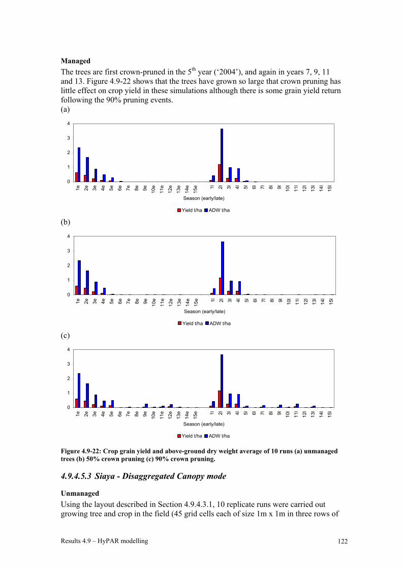
Results 4.9 – HyPAR modelling 122
Managed The trees are first crown-pruned in the 5th year (‘2004’), and again in years 7, 9, 11 and 13. Figure 4.9-22 shows that the trees have grown so large that crown pruning has little effect on crop yield in these simulations although there is some grain yield return following the 90% pruning events. (a)
0
1
2
3
4
1e 2e 3e 4e 5e 6e 7e 8e 9e 10e
11e
12e
13e
14e
15e 1l 2l 3l 4l 5l 6l 7l 8l 9l 10l
11l
12l
13l
14l
15l
Season (early/late)
Yield t/ha ADW t/ha
(b)
0
1
2
3
4
1e 2e 3e 4e 5e 6e 7e 8e 9e 10e
11e
12e
13e
14e
15e 1l 2l 3l 4l 5l 6l 7l 8l 9l 10l
11l
12l
13l
14l
15l
Season (early/late)
Yield t/ha ADW t/ha
(c)
0
1
2
3
4
1e 2e 3e 4e 5e 6e 7e 8e 9e 10e
11e
12e
13e
14e
15e 1l 2l 3l 4l 5l 6l 7l 8l 9l 10l
11l
12l
13l
14l
15l
Season (early/late)
Yield t/ha ADW t/ha Figure 4.9-22: Crop grain yield and above-ground dry weight average of 10 runs (a) unmanaged trees (b) 50% crown pruning (c) 90% crown pruning.
4.9.4.5.3 Siaya - Disaggregated Canopy mode
Unmanaged Using the layout described in Section 4.9.4.3.1, 10 replicate runs were carried out growing tree and crop in the field (45 grid cells each of size 1m x 1m in three rows of

Results 4.9 – HyPAR modelling 123
15). The crop yields for the three rows are combined and averaged over the 10 runs to give an average figure for the yield as it varies with distance from the tree. Figure 4.9-23 illustrates these results at sample point 1m, 5m, 10m and 14m away from the tree and the total yield for the entire field (i.e. all 45 cells combined). Close to the tree the crop yield declines rapidly to zero after 5 years. At a distance of 10m from the tree, the crop continues to yield grain for approximately 13 years although the amount is small. Further from the tree (outside the range of the tree roots) the yield does not decline with time. The shaded bar in Figure 4.9-23 shows the total for the whole field and indicates that although the crop cannot grow under the tree, the farmer would obtain some crop product from this area of land.
Management options Figure 4.9-24 illustrates the effect of tree crown pruning (90%) on crop yield over the 15-year simulations. By comparison with Figure 4.9-23 crown pruning can be seen to increase the total yield in the later years by increasing the yield closer to the tree (darker bars) although yield away from the tree may be reduced. To examine the effects of root pruning, a simulation was carried out (10 replicate runs of 15 years as before) in which the tree root width parameter was reduced to 0.1. This means that the tree roots were restricted to a radius of 0.1 times the tree height. Figure 4.9-25 shows the crop grain yield at the same distances from a tree with the total for the field. Crop growth increases further than 1m away from the tree but this is not entirely due to the absence of tree roots – with restricted root growth the tree grows more slowly and reaches only 17m in height with a crown of radius 3.7m. With restricted roots and 90% crown pruning applied, the effects of the tree on the crop is reduced as shown in Figure 4.9-26.
0.00
0.20
0.40
0.60
0.80
1.00
1.20
1.40
1e 2e 3e 4e 5e 6e 7e 8l 9e 10e 11e 12e 13e 14e 15e 1l 2l 3l 4l 5l 6l 7l 8l 9l 10i 11l 12l 13l 14l 15l
Year (early/late season)
Crop grainyield (t/ha)
1 m 5m 10m 14m Total for field
Figure 4.9-23: Crop grain yield at sample distances from an unmanaged tree (1m, 5m, 10m and 14m) with the total for the field.

Results 4.9 – HyPAR modelling 124
0.00
0.20
0.40
0.60
0.80
1.00
1.20
1.40
1e 2e 3e 4e 5e 6e 7e 8l 9e 10e 11e 12e 13e 14e 15e 1l 2l 3l 4l 5l 6l 7l 8l 9l 10i 11l 12l 13l 14l 15lYear (early/late season)
Crop grainyield (t/ha)
1 m 5m 10m 14m Total for field
Figure 4.9-24: Crop grain yield at sample distances from a pruned tree (1m, 5m, 10m and 14m) with the total for the field. The tree had 90% crown pruning applied in years 5, 7, 9, 11 and 13 on day 60.
0.00
0.20
0.40
0.60
0.80
1.00
1.20
1.40
1e 2e 3e 4e 5e 6e 7e 8l 9e 10e 11e 12e 13e 14e 15e 1l 2l 3l 4l 5l 6l 7l 8l 9l 10i 11l 12l 13l 14l 15l
Year (early/late season)
Crop grainyield (t/ha)
1 m 5m 10m 14m Total for field
Figure 4.9-25: Crop grain yield at sample distances (1m, 5m, 10m and 14m) from a tree with the total for the field. The tree roots had their growth restricted to a radius of 0.1 times the tree height.
0.00
0.20
0.40
0.60
0.80
1.00
1.20
1.40
1e 2e 3e 4e 5e 6e 7e 8l 9e 10e 11e 12e 13e 14e 15e 1l 2l 3l 4l 5l 6l 7l 8l 9l 10i 11l 12l 13l 14l 15l
Year (early/late season)
Crop grainyield (t/ha)
1 m 5m 10m 14m Total for field
Figure 4.9-26: Crop grain yield at sample distances (1m, 5m, 10m and 14m) from a tree with the total for the field. The tree roots had their growth restricted to a radius of 0.1 times the tree height and the tree crown was pruned by 90% in years 5, 7, 9, 11 and 13 on day 60.
4.9.4.6 Reduced Rainfall at Siaya The daily weather generator within HyPAR has two input variables controlling rainfall, the fraction of wet days per month and the rain per wet day. Reduced rainfall for a given site can therefore be achieved by decreasing either variable separately or both simultaneously. Reducing the number of wet days per month means that the plants experience more days with no rain at all whereas reducing the rain per wet day results in less intense rain events. The stress placed on the tree and crop growth will be different so the plants will respond in different ways.

Results 4.9 – HyPAR modelling 125
In order to simulate the possible impact of climate change at Siaya, or to explore the effect of management on agroforestry in drier locations a set of simulations were carried out with the Siaya environment and reduced rainfall (see section 4.9.4.1.1). In one case the rain fall amounts were reduced and in the other simulations the number of wet days was reduced while in both cases the average annual total rainfall was approximately 830mm. Figure 4.9-27 shows crop grain yield for (a) standard rainfall (b) 20% reduction in rain per wet day (c) 20% reduction in number of wet days per month. (a)
0.0
0.2
0.4
0.6
0.8
1.0
1.2
1.4
1e 1l 2e 2l 3e 3l 4e 4l 5e 5l 6e 6l 7e 7l 8e 8l 9e 9l 10e 10
l11
e 11l
12e 12
l13
e 13l
14e 14
l15
e 15l
Crop only Yield t/ha Prune 90% Yield t/ha Prune 50% Yield t/ha Unmanaged Yield t/ha
(b)
20% reduction in rain per wet day
0.00.20.40.60.81.01.21.4
1e 1l 2e 2l 3e 3l 4e 4l 5e 5l 6e 6l 7e 7l 8e 8l 9e 9l 10e 10
l11
e 11l
12e 12
l13
e 13l
14e 14
l15
e 15l
Crop only Yield t/ha Prune 90% Yield t/ha Prune 50% Yield t/ha Unmanaged Yield t/ha
(c)
20% reduction in number of wet days
0.00.20.40.60.81.01.21.4
1e 1l 2e 2l 3e 3l 4e 4l 5e 5l 6e 6l 7e 7l 8e 8l 9e 9l 10e 10
l11
e 11l
12e 12
l13
e 13l
14e 14
l15
e 15l
Crop only Yield t/ha Prune 90% Yield t/ha Prune 50% Yield t/ha Unmanaged Yield t/ha
Figure 4.9-27: Mean crop grain yield (t/ha) over 10 simulation runs in uniform mode each of 15 years with unmanaged trees or 50% and 90% crown pruning in years 5, 7, 9, 11 and 13. (a) Standard rainfall (b) 20% reduction in rain per wet day (c) 20% reduction in number of wet days per month.

Results 4.9 – HyPAR modelling 126
The amount of water available to the crop during the growing season depends on several factors including rainfall seasonality, frequency and intensity and soil draining properties. In these simulations (Figure 4.9-27) the average crop yield in the standard run is 0.63 t/ha (a, hatched bars) and a 20% drop in rainfall by reducing the rain intensity leads to a corresponding drop in yield to 0.48 t/ha (b, hatched bars). However, a 20% reduction in rainfall created by reducing the rainfall frequency leads to a small increase in yield to 0.64 t/ha (c, hatched bars). This may be due to reduced evaporation from the soil, a different infiltration pattern into the soil or timing of the rainfall events relative to the crop season. When trees are added to the simulation (unmanaged or crown pruned at 50% and 90% as before) a similar pattern is seen – the reduced rainfall intensity leads to a 20% drop in yield whereas a reduced rainfall frequency increases crop yield by up to 45% compared with the sole crop simulations. Movement of water through the soil also influences nutrient availability making comparisons between sites very complex.

Results 4.9 – HyPAR modelling 127
4.9.5 Tree and Crop Parameters Table 4.9-7: Tree species parameters for Grevillea
Value Name Description 0.65 kpar PAR extinction coefficient 0.48 ksw SW extinction coefficient 0.05 rhop PAR reflection coefficient 0.2 rhos SW reflection coefficient 1 fturn turnover rate of foliage (proportion yr-1) 0.01 wturn turnover rate of wood (proportion yr-1) 2 rturn turnover rate of fine roots (proportion yr-1) 25.524 sla specific leaf area (m2 kg C-1) 0.033 bark ratio of dbh to bark thickness (mm-1) 4208 lasa ratio between leaf area and sapwood area (m2m-2) 33.918 ah Allometry a parameter for dbh (m) to height (m) 0.374 bh Allometry b parameter for dbh (m) to height (m) 0.464 ch Allometry c parameter for crown diameter (m) 0.22 stf proportion of woody biomass below ground (proportion) 1 rlratio biomass ratio between fine roots and foliage 0.5 frcoeff foliage nitrogen retranslocation coefficient (proportion) 1 rrcoeff fine root nitrogen retranslocation coefficient (proportion) 0.05 rmf reserve mobilisation factor (proportion) 220.43 woodd mean wood and bark specific gravity (kg C m-3) 0.58 formf tree form factor (dimensionless) 0.145 fsr ratio between C:N ratios of foliage and sapwood+ 0.86 frr ratio between C:N ratios of foliage and fine roots 0.142 live proportion of sapwood alive (proportion) 0.67 storef maximum proportion of live sapwood used as C storage 0.036 nupc N uptake parameter (m2 kg C-1 d-1) 1433 ngr maximum leaf conductance to CO2 (m s-1) 4.81E-05 gmin cuticular conductance to CO2 (m s-1) 0.67 pruba proportion of foliage nitrogen bound in Rubisco (proportion) 9.13 nrc proportion of foliage nitrogen bound in chlorophyll (proportion) 0.04 d_leaf leaf characteristic dimension (m)
3 ptype potential species vegetation type (1=grass;2=EVGR;3=CD;4=DD;5=DDG)
0.75 rgf factor to allow for growth respiration (proportion) 0.1 wmf factor for calculating minimum wood mass increment 1.5E-07 TreeRWL root weight per unit length (kg cm-1) 0.125 roothd Factor for root distribution half depth 0.5 rootdf Factor for rooting depth from height

Results 4.9 – HyPAR modelling 128
0.125 roothw Factor for root distribution half width 0.5 rootwf Factor for rooting width from dbh Table 4.9-8: Crop cultivar parameters for ‘maize’: Full descriptions are given in the HyPAR manual (Mobbs et al. 2001).
Value Name Value Name
3.01 VERTEST 0.4 Lrollmax
54 CULTNUM 24 SLA1
0.1 minFL 20 SLA2
0.8 maxFL 0.5 maxPlantArea
0.1 maxFH 1 Lifec
0.25 OFBG1 2.5 Photosynth1
0.2 TransPot 2.3 Photosynth3
0.05 DayTransPot 0.47 K
9 Germination 0.009 qD
15 Juvenile 17 GNC
7 GrainSetTime 0.042 maxGW
23 PartitionTime 20 RDmin
7 Tb 45 RRmax
48 Tm 5 RLVmax
24 Tbplateau 6 emRWLfactor
41 Tmplateau 4 emRDfactor
0.1 GS1ttFactor 1.5E-07 RWLfactor
0 GS3ttFactor 12 FineRoot
365 GS1tt 0.1 maxUptakeRate
680 GS2tt 250 Rdist
609 GS3tt 1800 maxRdepth
4 STindex 45 PWiltP
0.5 Recovery 0.95 WLsat
0 STransReduct 2 WLdamage
0.7 SLAstress 1.1 WLrecover
0.09 LeafStress 5 WLsuscept
0.4 RstressFBG 0.1 WLdeath
0.8 maxRstress 0 FractRoot

Results 4.9 – HyPAR modelling 129
4.9.6 References Arah, J., and M. Hodnett. 1997a. Approximating soil hydrology in agroforestry
models. Agroforestry Forum 8:17-20.
Arah, J., and M. Hodnett. 1997b. Chapter 4: Handling soil hydrology in agroforestry models. Pages 36-42 in Annual Report (July 1996- June 1997) Agroforestry Modelling and Research Co-ordination Project Report to DFID-FRP. Centre for Ecology & Hydrology.
Bradley, R. G., and N. M. J. Crout. 1996. PARCH-User Guide. Tropical Crops Research Unit University of Nottingham.
Brooks, R. H., and A. T. Corey. 1964. Hydraulic properties of porous media. 3, Civil Engineering Dept. Colorado State Univ., Fort Collins, Colorado.
Cannell, M. G. R., D. C. Mobbs, and G. J. Lawson. 1998. Complementarity of light and water use in tropical agroforests - II. Modelled theoretical tree production and potential crop yield in arid to humid climates. Forest Ecology and Management 102:275-282.
Friend, A. D. 1998. Parameterisation of a global daily weather generator for terrestrial ecosystem modelling. Ecological Modelling 109:121-140.
Friend, A. D., A. K. Stevens, R. G. Knox, and M. G. R. Cannell. 1997. A process-based, terrestrial biosphere model of ecosystem dynamics (Hybrid v3.0). Ecological Modelling 95:249-287.
Geng, S., F. P. d. Vries, and I. Supit. 1986. A simple method for generating daily rainfall data. Agricultural and Forest Meteorology 36:363-376.
Lott, J. E., C. R. Black, and C. K. Ong. 1998. Comparison of output from HyPAR with observed maize yields in CIRUS. R5810, Nottingham University, Sutton Bonnington.
Mobbs, D. C., M. G. R. Cannell, N. M. J. Crout, G. J. Lawson, A. D. Friend, and J. Arah. 1998. Complementarity of light and water use in tropical agroforests - I. Theoretical model outline, performance and sensitivity. Forest Ecology and Management 102:259-274.
Mobbs, D. C., G. J. Lawson, A. D. Friend, N. M. J. Crout, J. Arah, and M. G. Hodnett. 2001. HyPAR v4.5 Technical Manual. Technical Manual Centre for Ecology and Hydrology, Edinburgh.
Richardson, C. W., and D. A. Wright. 1984. WGEN: A Model for Generating Daily Weather Variables. ARS-8, U.S. Department of Agriculture, Agricultural Research Service.

Results 4.9 – HyPAR modelling 130
Tefera, A. 2004. Crown and root pruning of four year old boundary trees at Siaya and Nyabeda in western Kenya: socioeconomics, utilization of soil water, and maize and wood yields. Sokoine University of Agriculture, Tanzania. 277pp.

4.10 Socioeconomic modelling 131
4.10 Socio economic analysis of pruning in Kenya
Anna Maria Giacomello (CEH Wallingford)
4.10.1 Summary The main finding of the economic analysis is that it is essential for farmers to diversify their sources of income through agroforestry and the application of severe pruning is necessary to reduce competition. Although the agroforestry scenario with severe pruning provides the lowest returns with respect to the other agroforestry and forestry scenarios, it is an attractive option for subsistence farmers since it reduces the risk for farmers to lose their yield, and the returns over the 15 year rotation are higher than the arable (crops only) system. For subsistence farmers, planting trees alone is an unsustainable option as they need to have either access to credits or other sources of income to be able to support themselves during the rotation period. If they had access to credits, forestry and agroforestry systems would become less profitable options as the interest rate increases. The possible solution in this case would be to shorten the rotation or to select trees with a shorter optimal rotation. It was clear that the more crop prices are unstable, the more agroforestry systems provide financial security to the farmer. However, the profitability of agroforestry is very sensitive to changes in tree prices. To avoid the collapse of tree prices during a drought when everyone begins to sell the same trees on the local market, it is important for farmers to diversify the type of trees grown so that a reduction in value in one tree is compensated by the value of another one. Root pruning has lower marginal additional costs than crown pruning and these costs are exceeded by the benefits from a higher crop yield. Such a practice would integrate easily in farming routine as farmers do not need to have special plans for root pruning; they could do it when they prepare their land for planting crops (Tefera 2002). Most of the farmers from the different study areas are aware of the advantage of agroforestry. Farmers in different areas selected different types of trees, which may reflect differences in their food security although a number of other factors could also be involved. In drought-prone Kibwezi, farmers often select fruit trees, which provide continuous returns, whereas Siaya farmers often plant trees that have long-term returns in the form of poles and timber. Depending on the type of trees grown, farmers have a different propensity towards practising severe pruning. Farmers choosing to grow fruit trees next to crops cannot crown prune as this reduces fruit production. In this instance, farmers must accept a certain level of trade-off between fruits and crop yield, making them even more vulnerable to droughts. Farmers growing timber trees see a twofold advantage in pruning, not only do they reduce the tree competition with crops but also they obtain firewood and actually a better timber bole. The main problem for subsistence farmers is that they do not have enough savings and access to a cash economy to wait for the revenues from timber in few years time; the risk of losing their crop yield is too high for them. The risk increases as the crop plot available for farmers reduces.

4.10 Socioeconomic modelling 132
4.10.2 Introduction Kenya’s population is concentrated in rural areas where rain-fed agriculture is the main occupation. However, only a small proportion of the country (less than 20%) is suitable for rain-fed crops; in most areas agricultural production is very risky due to the erratic amount of rainfall. Increasing demand for agricultural products and land, driven by high population growth, has pushed farming towards more marginal areas even less suitable for rain-fed agriculture. In these areas of especially high risk of crop failure, it is especially important for farmers to diversify their sources of income to be able to cope with droughts. One option to diversify investments is agroforestry, which provides not only a crop yield in the short term but a longer term added income from tree harvests. However, increasing competition between trees and crop as trees age, reduces crop yields which may not be desirable for farmers who rely on regular crop harvests. Therefore, for the agroforestry system to be attractive it has to ensure a minimum constant crop yield throughout the rotation period because lack of savings and difficulty in accessing the cash economy make it difficult for farmers to cope with lower yields. One way to make agroforestry more productive and thus more attractive to farmers is to reduce competition through crown and root pruning. This process reduces the shade and water competition between trees and crop, leading not only to better yields but to additional returns in the form of firewood, charcoal and improved bole quality. An economic model was constructed to represent an agro-forestry system in terms of farmers’ cash flow and the impact that different intensities of pruning would have on the farmers’ income. Sensitivity analysis was carried out to assess the way in which economic and biophysical variations could affect the farmer’s decision to implement an agroforestry system with or without pruning with respect to the arable system. In the next section an overview of the Kenyan economy is presented, with particular emphasis given to the agricultural sector contribution to the national economy, the current constraints, and the way forward. The economic model structure is explained in section 4.10.3; results of the simulations and sensitivity analysis are then discussed. A summary of results of the survey carried out in Siaya can be found in Appendix C. A more extensive presentation of survey data is provided in 4.1.1.
Overview of Kenyan economy Although Kenya currently has the largest economy in East Africa, Uganda and Tanzania are both providing increasingly serious competition. Furthermore, the economic situation in Kenya has deteriorated over the past decade because of the slow pace of structural reform, failure to sustain prudent macro-economic policies, and a deteriorating infrastructure and inefficient parastatal sector. As a consequence poverty has increased11 and social indicators deteriorated12.
11 In 2000 it has been estimated that 50% of population is below the poverty line (source: CIA 2003) 12 The Kenya population and housing census in 1999 have highlighted that life expectancy at birth has reduced over the last 10 years from 61.9 years to 56.6 years (Source Central Bureau of Statistics 2003); and in 1998 the UNICEF representative in Nairobi revealed that Kenya’s child mortality rate has increased by over 20% since the early 1990s, a consequence of declining health services, widespread poverty and the spread of AIDS/HIV infection.

4.10 Socioeconomic modelling 133
In 2000, for the first time since independence in 1963, Kenya’s economy contracted with a GDP growth rate falling to - 0.2%. The Central Bank of Kenya highlighted the prolonged drought and severe power rationing as the major factors contributing to this slow down in the economy. The bank pointed out that poor infrastructure, the continued mismanagement of key agricultural institutions and insecurity have also played a role. Despite the return of heavy rains in 2001, Kenya’s economic growth has been limited to 1.2% because of weak commodity prices, endemic corruption, and low investment. In contrast the growth rate in neighbouring Uganda and Tanzania has been around 5%. Growth fell still further to 1.1% in 2002 because of erratic rains, and uncertainty about the general election. The situation was reflected by: a) low demand for imports; b) low demand for credit; and c) donors waiting for Kenya’s decision before releasing funds.
Table 4.10-1 - Real GDP growth rate 2000 2001 2002 Kenya - 0.2% 1.2% 1.1% Tanzania 5.1% 5.6% 5.8% Uganda 5% 5.6% 5.7%
Source: Central Bureau of Statistics 2003 Although the contribution of agriculture to the economy of Kenya has fallen over the past 40 years it still accounts for around 26% of GDP and 18% of waged employment in both agriculture and agro-industries. Almost half of all output is for subsistence and not marketed. The sector output recorded a growth of 0.7% in 2002 compared to 1.3% in 2001; this decline was mainly due to poor weather conditions that led to a decline in the production of tea and coffee. However, food security was supported by previous stocks. The growth in the agricultural sector was due to an increase in horticultural exports from 98.9 thousand tonnes in 2001 to 121.1 thousand tonnes in 2002. The expansion of the horticultural sector since the 1980s has been impressive, particularly over the past five years during which the rate of growth has doubled. In 1999 it became the second largest export earner after tea, with flowers making up the largest contribution.
Table 4.10-2 – Sectoral Share of GDP (%) Sector 1998 1999 2000 2001 2002 Agriculture, Fishing & Forestry 27 26.9 26.5 26.5 26.4 Industry 19.2 19.1 18.9 18.8 18.8 Services 53.8 53.9 54.6 54.7 54.8 Total 100 100 100 100 100 Source: Central Bureau of Statistics 2003 Kenya is the most industrially developed country in East Africa. Industry accounts for 19% of GDP in 2002 and employs 8% of the labour force. The sector is dominated by food-processing industries, most of which are located in the urban centres. The sector faces a number of difficulties, notably a weak infrastructure, rising costs and import competition. During the 1990s the government’s industrial policy shifted away from import substitution and protectionism towards liberalisation and privatization. In practice, this has led to the gradual removal of tariff barriers, encouraging competition and recognizing the role of the informal Jua Kali13 industrial sector. 13 This term is used to indicate the informal sector. Jua kali means ‘hot sun’ in Kiswahili and refers to the very small-scale entrepreneurs who typically work outdoors under the hot sun for want of a shed or workshop.
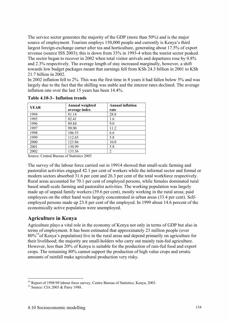
4.10 Socioeconomic modelling 134
The service sector generates the majority of the GDP (more than 50%) and is the major source of employment. Tourism employs 150,000 people and currently is Kenya’s third largest foreign-exchange earner after tea and horticulture, generating about 17.5% of export revenue (source ISS 2003); this is down from 33% in 1993-4 when the tourist sector peaked. The sector began to recover in 2002 when total visitor arrivals and departures rose by 0.8% and 2.3% respectively. The average length of stay increased marginally, however, a shift towards low budget packages meant that earnings fell from KSh 24.3 billion in 2001 to KSh 21.7 billion in 2002. In 2002 inflation fell to 2%. This was the first time in 8 years it had fallen below 5% and was largely due to the fact that the shilling was stable and the interest rates declined. The average inflation rate over the last 15 years has been 14.4%.
Table 4.10-3– Inflation trends
YEAR Annual weighted average index
Annual inflation rate
1994 81.14 28.8 1995 82.41 1.6 1996 89.84 9.0 1997 99.90 11.2 1998 106.53 6.6 1999 112.65 5.8 2000 123.86 10.0 2001 130.99 5.8 2002 133.56 2
Source: Central Bureau of Statistics 2003 The survey of the labour force carried out in 19914 showed that small-scale farming and pastoralist activities engaged 42.1 per cent of workers while the informal sector and formal or modern sectors absorbed 31.6 per cent and 26.3 per cent of the total workforce respectively. Rural areas accounted for 70.1 per cent of employed persons, while females dominated rural based small-scale farming and pastoralist activities. The working population was largely made up of unpaid family workers (39.6 per cent), mostly working in the rural areas; paid employees on the other hand were largely concentrated in urban areas (33.4 per cent). Self-employed persons made up 23.8 per cent of the employed. In 1999 about 14.6 percent of the economically active population were unemployed.
Agriculture in Kenya Agriculture plays a vital role in the economy of Kenya not only in terms of GDP but also in terms of employment. It has been estimated that approximately 23 million people (over 80%15of Kenya’s population) live in the rural areas and depend primarily on agriculture for their livelihood; the majority are small-holders who carry out mainly rain-fed agriculture. However, less than 20% of Kenya is suitable for the production of rain-fed food and export crops. The remaining 80% cannot support the production of high value crops and erratic amounts of rainfall make agricultural production very risky.
14 Report of 1998/99 labour force survey, Centre Bureau of Statistics, Kenya, 2003. 15 Source: CIA 2003 & Parry 1988.

4.10 Socioeconomic modelling 135
In Kenya, 90% of rain falls within two distinct wet seasons, which represent the two growing seasons. However, both seasons are highly variable and the date at which they begin, and the duration and amount of rain, fluctuate widely from season to season. The low level of technology makes each of the cultivation practices required for successful crop production extremely labour-intensive. In certain areas labour can be a constraint to improving agricultural production as the peak demand for labour to carry out different types of operations arises almost simultaneously, particularly in March when planting and harvesting can occur at the same time. In addition, parents increasingly recognise the value of education, so there is a reduction in child labour on the farm, and those who have been educated beyond primary school rarely return to work on the farm. The economic situation of Kenya is particularly vulnerable to climate variability as a severe drought may not only have a negative impact at livelihood level but also on the entire economy of the country, given that more than a quarter of GDP is from agriculture. The types of household that are least vulnerable to drought are those with access to a variety of non-agricultural market exchanges. They will experience the effect of drought through the local and national economy as it affects prices and food supply in the local markets. However, climate variability has a direct impact on households that rely on their own production to meet their subsistence needs. For those households in this category with small holdings, poor soils, and insufficient labour and capital, the effect of drought may be acute. In addition to climatic vulnerability Kenya is facing a high population growth, which, despite declining over the last decade, still stands at more than 2%16 per year. One of the major consequences of population growth is that as the demand for both agricultural products and land rises, the size of holding tends to reduce and the number living on marginal lands increases. This process further exposes large numbers to the risk of reduced production caused by the low productivity of these areas, creating an even more vulnerable situation for Kenya’s economy. Better policy at macro level and better methods and systems at micro level are needed to improve the reliability of production and yield in these areas.
Macro-economic policies Despite agriculture being the crucial sector for the economies of many African countries, it carries an implicit and explicit burden. The implicit burden is caused by those macro-economic policies designed to promote industrial activities (by means of tariff protection, quotas, subsidies, government investment, etc.) and the resulting overvalued exchange rates. The explicit burden consists of such things as taxes on agricultural exports and major price disparities where marketing boards are responsible for buying and selling. These and other price interventions have resulted in unfavourable internal terms of trade between agriculture and other sectors. Rather than sectoral policies, the major determinants of agricultural prices have been exchange rates, trade and tariff policies. Protection of the industrial sector has raised the prices of inputs used in agricultural markets, while taxation and currency overvaluation have
16 Population annual growth rate has slowed down, in 1970-90 it was 3.6% and now in 1990-2001 is 2.6% (Unicef 2003). It has been estimated that the growth rate will drop down to 1.8% in the next 10 years without taking into account of AIDS, with AIDS the growth has been estimated to be 0.6% (source: ISS 2003).

4.10 Socioeconomic modelling 136
led to low prices for farm products. The anti-agricultural bias in the macro-policy in most of the developing world has left a clear mark on the sector’s performance. In fact, advances in productivity growth slowed down in much of the 1970s and 1980s and the gap between agricultural and other income continued to widen. As a much larger population lives on agriculture returns, macro-economic policies targeted to strengthen the agriculture sector are urgently required if poverty reduction targets have to be met.
Micro-economic activities At the farm level it is important to introduce farming practices that increase farmer financial security. Agroforestry systems bring this benefit by enabling farmers to diversify their investments in the short and long term thus reducing the financial risk. In general, diversification of investments provides financial advantages, although it also introduces the need for additional management expertise to deal with the added complexity of the system. Three general economic benefits are typically associated with agro-forestry: spreading (sharing) of fixed costs because of the joint-production relationship; reducing the initial time period required to produce income from land devoted exclusively to tree production; and diversifying income sources, in effect spreading the risk generally associated with a monoculture, especially in areas where crop failure is frequent. To be of economic interest agro-forestry has to ensure that over the rotation period the benefits from each additional tree are greater than the benefits lost by the reduction in crop yield due to shade and water competition with trees and reduced space for crop planting. By adopting pruning practices such as crown and root pruning farmers can reduce the water and shade competition between trees and crop and have added value in terms of firewood and better quality of poles. From an operational standpoint, agro-forestry to some extent increases flexibility in agricultural operations since many pruning practices may be delayed with little or no detrimental effect until free time is available; whereas activities such as crop sowing and weeding cannot be delayed. The aim of the economic model described in section 4.10.3 is to examine whether and in what circumstances pruning practices are economic for farmers. If this is the case, the implementation of agroforestry systems would find a wider application since until now it has been constrained by the threat of farmers losing crop yield and in the inability to manage tree and crop competition.
Overview of case study in Kenya The economic model and analysis focuses on the Kenya site at Siaya. Out of the 8 sites where field work was carried out, Siaya was chosen because of its average climate condition with respect to the other sites and the availability of more complete sets of climate, soil, tree, crop and economic data. Siaya is located in the Nyanza province in western Kenya. In Siaya as the rest of Kenya there is a land shortage problem, so subsistence farmers cannot afford to allocate part of their land only to trees. The option left for them is to plant trees next to crop and prune them to reduce the water and shade competition between trees and crop. However, in Siaya although farmers had noted a reduction in crop yield next to trees, they did not know how to manage the competition. They coped with the problem by either accepting a reduction in crop yield or

4.10 Socioeconomic modelling 137
removing the trees from the land increasing in both cases their economic vulnerability (Tefera 2002). From a welfare point of view household heads in Siaya have a mean monthly wage income lower than average for rural household head (see Table 4.10-27 page 172). On average in Siaya 57 % of households’ income is generated from their own farming activities, this is more than the average rural household (48%). In Siaya farmers spend almost half of their income to buy food (41%), especially maize, meat and sugar.
4.10.3 Economic model
Introduction One of the aims of this project was to design an economic model able to represent an agro-forestry system in terms of farmers’ cash flow and the impact that different intensities of pruning would have on farmers’ income. The model has been based on the BEAM model and adapted to suit the data availability and pruning practice considered in this project. The model combines the outputs from HyPAR (i.e. crop yield) with the economic data obtained from the local survey and relevant literature. In the current version of HyPAR the simulation of root pruning has been difficult to implement, so the economic model as HyPAR focuses on the effect of crown pruning only. The general aims of this economic model are to: Compare, at a field level, profitability and cash-flow of agroforestry with respect to the returns and cash flow that a farmer could get by growing only crops or trees. Determine the effects that pruning practices have on an existing farm in terms of production, profitability and cash-flow. The model calculates the net margins for each of the farming systems. The net margins are derived by subtracting variable costs (i.e. seeds, fertilisers and water) and fixed costs (labour and tools) from the revenue17. Both the annual and the cumulative net margins for each of the farming systems are provided. The approaches to derive the annual benefits associated with crop production are mainly two: the annual net margins and the annual discounted net margins. The first approach derives the annual benefit by dividing the total net margins over the production cycle by the length of the rotation in years. However, this approach does not consider the timing of the expenditures and revenues, which usually do not occur at the same time. Therefore this could lead to a biased estimation of the annual benefits. This bias depends on how long it takes to gain the first returns from the plantation. For example, forestry plantations have a long rotation and the harvest occur only at the end of the rotation compared to field crops where harvests occur annually. The second approach (annual discounted net margins) takes account of the timing by discounting18 the cash flow over the entire rotation and it divides them by the length of the rotation in years. The annual discounted net margins approach estimates the present worth of a crop that will be harvested in the future. Due to lack of information about the future trends in prices, the annual discounted net margins can be calculated by either using constant prices or projection trends derived observing the past; these are strong assumptions. In the model 17 By calculating the revenue they would get by selling their yield, even if farmers are consuming all their harvest, we are calculating their imputed income. 18 See APPENDIX B for explanation of discounting.

4.10 Socioeconomic modelling 138
prices have been set constant, due to lack of data on price trends. The model calculates both the annual net margins and the annual discounted net margins. The cumulative net margins can be calculated by either including the discounting rate (the cumulative discounted net margins obtained by calculating the net present value of the cash flow of each of the farming systems) or not (by simply summing up the returns from each year of the rotation). The model calculates both of them. However we are presenting only the annual net margins as they can be compared more easily to the annual household income.
Model structure The model had been constructed using an Excel spreadsheet and it comprises 8 worksheets. Worksheet Name Data 1 Options Input data 2 Results Output data 3 Scenarios Input data 4 Crop biophysical data Input data 5 Tree biophysical data Input data 6 Financial data Input data 7 Hectare results Output data 8 Farm results Output data
In the sections that follow the contents of each worksheet are described in more detail.
Worksheet 1 – OPTIONS In this worksheet the user can change the following options: Size of the farm: The user can set the size of the farm. In the case of Siaya the farm has been set at
2 hectares as from the survey it came out that on average farmers cultivate 4.9 acres.
Scenario: This cell is set as a drop down menu from which the user can select a scenario out of 13 possible options; see worksheet 3 for the list of scenarios.
Percentage of land that is cultivated with crops:
This is proportional to the number of trees that are planted on a hectare; currently with 179 tree per hectare the proportion of land cultivated has been set at 90%.
The discounting rate: The initial value of the discounting rate has been set at 3% and then at different rates to carry out some sensitivity analysis.
Crop type: This cell is organised as a drop down menu; it could contain different crops, at present it is set to different prices of maize: a) “maize” with this option the price is set at KSh18/kg (source: Mulatya 2000); b) “maize pr av” in this case the price is set at KSh 11.6/kg, this is an average of the monthly prices of maize over one year (source: Kiptot 2002); and c) “maize pr ses” in this case the maize price is set at KSh 7.5/kg if the crop is harvested early in the year or if at KSh 18.9/kg if it is a late harvest (source: Kiptot 2002).
Tree species: This cell is organised as drop down menu; it could contain different trees, but for the moment is used to set different value of trees. The set of data available were the average price of Melia at different tree age, but there was not relation to the m3; so to convert the price available to a m3 price we had to make some assumptions (see Appendices APPENDIX A - Prices (maize, trees)). The option “Melia jk” lists the price of Melia tree without relation to the volume (source: Mulatya 2000); the option “Melia pr (m3)” lists prices that are expressed in terms of volume; this has been obtained by using “Melia jk” prices and the standing tree volume from HyPAR simulation (Appendices APPENDIX A - Prices (maize, trees)).
4.10 Socioeconomic modelling 139
Crop price reduction: This cell is organised as a drop down menu; the user can select from a range of crop price reduction only when the crop type cell is set at the “maize” option.
Tree price reduction: This cell is organised as a drop down menu; the user can select from a range of tree price reduction only when the cell on tree specie is set at the “Melia pr (m3)” option.
By changing the options above the user can see in the Result worksheet the effects of these choices in terms of profitability and production. The results of some of the possible changes are presented in sections 4.10.4 and 4.10.5.
Worksheet 2 - RESULTS In this worksheet the agroforestry returns at farm scale are compared with those of forestry and agriculture (see Figure 4.10-1). The returns are expressed in terms of both actual annual net margins and annual discounted net margins. For each of the farming systems, the numbers of years during which the farmers are in loss are counted. In the agricultural system section, the average annual crop yield and the number of years without any crop yield are also shown. In the forestry system section we have listed the total harvested timber volume, the annual average carbon sequestered, the total pruning and firewood obtained over the 15 years. In the particular case of scenario 5 in Figure 4.10-1, the farmer is growing both trees and crops on his land, but he is leaving the trees unmanaged. The total firewood in the ‘tree result’ section is obtained by the farmer at the end of the rotation period then he fells his trees.

4.10 Socioeconomic modelling 140
Figure 4.10-1 – Example of Worksheet 2 results SCENARIO 5
CROP RESULTS TREE RESULTSin 2 hectare over 15 years in 2 hectare over 15 years
Annual discounted net margin 1,724- Ksh/yr Annual discounted net margin 40,755 Ksh/yr
Annual net margins 3,216- Ksh/yr Annual net margins 61,861 Ksh/yr
Average annual Crop yield 0.5 t/yr Number of yr at loss 14 no
Number of yrs with no crop 9 no Total harvested volume 481 m3
Number of yr at loss 10 no Average carbon sequestered 58,937 Kg C/yr
Total firewood 42,441 Kg
AGROFORESTRY RESULTSin 2 hectare over 15 years
Annual discounted net margin 39,032 Ksh/yr
Annual net margins 58,645 Ksh/yr
Number of yr at loss 10 no
Worksheet 3 - SCENARIOS This worksheet shows in more detail the characteristics of the 13 scenarios used to analyse the impact of average and severe crown pruning on farming income. However the model is designed so that it can contain up to 37 scenarios. The first scenario represents the situation where farmers grow only crops on their farm. The scenarios, which in the table below are highlighted in green, are those referring to farms where only forestry systems are carried out; and the scenarios, which in the table below are highlighted in orange, are those referring to agroforestry systems. HyPAR has been run assuming a tree density of 179 trees per hectare. The scenarios from 1 to 7 are based only on HyPAR outcomes, while scenarios 8 to 13 adjust the HyPAR biophysical outcomes to include expert judgments based on actual farm yields. Pruning is carried out after year 5, every 2 years. The HyPAR simulations show a limited crop yield response to crown pruning, although field studies carried out in the same area do show improved crop yields after crown pruning. Based on these findings, it has been assumed that the total crop yield over the 15 years when the trees are crown pruned at 50%, is 40% higher than when trees are unmanaged; when the trees are crown pruned at 90% the crop yield is 80% higher than when trees are unmanaged. Scenario 8, 9, 12 and 13 are based on these assumptions.

4.10 Socioeconomic modelling 141
Table 4.10-4 – List of pre-set scenarios
Scenario Type of system Crown
% Root
%
Tree density
(tree/ha) Felling at 4yr
Felling at 7yr
Felling at 15yr
Re-planting
1
Crop only 0 0 0 0 0 0 0
2 Tree only
unmanaged 0 0 179 0 0 100 0
3 Tree only -
50% pruned 50 0 179 0 0 100 0
4 Tree only –
90% pruned 90 0 179 0 0 100 0
5 Tree & Crop -
unmanaged 0 0 179 0 0 100 0
6 Tree & Crop - 50% pruned 50 0 179 0 0 100 0
7 Tree & Crop - 90% pruned 90 0 179 0 0 100 0
8
TC - 50% P - TM CNM 50 0 179 0 0 100 0
9
TC - 90% P - TM CNM 90 0 179 0 0 100 0
10
TC - 50% P - TNM CM 50 0 179 0 0 100 0
11
TC - 90% P - TNM CM 90 0 179 0 0 100 0
12
TC - 50% P - TCM 50 0 179 0 0 100 0
13
TC - 90% P - TCM 90 0 179 0 0 100 0
The standing volume of a tree reduces when tree are pollarded (shortening of bole, loss of branches), although, as already indicated, HyPAR does not reflect this because of difficulties with its structure. Consequently, it was decided to reduce the standing volume from HyPAR simulations by 20% over 15 years when trees are 50% pruned, and 50% when the trees are 90% pruned. Scenarios 10, 11, 12 and 13 consider these tree standing volume changes. Scenario 12 and 13 include both the crop and tree changes. The acronyms for scenarios 8 to 13 in column 2 of Table 4.10-4 stand for: No Acronym Description 8 TC - 50% P - TM
CNM Trees and crops are grown on the same plot; trees are pruned at 50%; HyPAR tree standing volume simulation have been modified; while HyPAR crop simulations have not been Modified.
9 TC - 90% P - TM CNM
Similar to the scenario above except for the pruning level that in this case is at 90%.
10 TC - 50% P - TNM CM
Trees and crops are grown on the same plot; trees are pruned at 50%; HyPAR tree standing volume simulation have not been modified; while HyPAR crop simulations have been modified.
11 TC - 90% P - TNM CM
Similar to the scenario above except for the pruning level that in this case is at 90%.
12 TC - 50% P - TCM Trees and crops are grown on the same plot; trees are pruned at 50%; both HyPAR tree standing volume and crop simulations have been modified.
13 TC - 90% P - TCM Similar to the scenario above except for the pruning level that in this case is at 90%.

4.10 Socioeconomic modelling 142
Worksheet 4 - CROP BIOPHYSICAL DATA This worksheet contains biophysical data on the 15 year annual crop yield (tonne/ha) obtained from the HyPAR model. HyPAR has been run assuming two crop seasons, one early season with a harvest between May and July and a late crop season with harvest between November and January. For the crop-only and the agroforestry scenarios there are two annual average crop yields: Crop yield s1 (the early harvest) and the Crop yield s2 (the late harvest). HyPAR has been run assuming that the only crop type grown in both seasons was maize; this matches the findings of the survey, where over 50% of farmers prefer to grow only maize next to trees. Scenarios 8, 9, 12, and 13 adjust the crop yield from the HyPAR simulation based on expert judgement (see Worksheet 3 section).
Worksheet 5 - TREE BIOPHYSICAL DATA This worksheet contains the following tree biophysical data from HyPAR for each rotation year: Tree height (metre) Stand volume (m3/tree) Carbon (kg C/tree) Trees harvested (tree/ha) Pruning volume (kg/tree) Tree volume has been obtained using the following formula:
58.02
2
∗∗
∗ heightdiamwπ
where diamw = dbh * (1.0 – (2.0 * 0.033) The tree species simulated in HyPAR is Grevillea which, except for Markhamia, is the most commonly grown tree in Siaya. The assumed rotation period is 15 years. Scenarios 10, 11, 12, and 13 adjust the standing tree volume from the HyPAR simulation based on expert judgement (see Worksheet 3 section)
Worksheet 6 - FINANCIAL DATA This is the worksheet containing the economic data. The worksheet is organised in three sections: 1) general financial data, 2) crop financial data; and 3) tree financial data. 1) General financial data This section includes labour costs and discounting rate. The data used for the labour cost are the following: 6.2 KSh/hr is the minimum wage for unskilled work for people below 18 yrs. (Source: Report on Labour force in Kenya 2003) 15 KSh/hr is based on survey results carried out in Kibwezi. 13.4 KSh/hr is based on the minimum wage rate set at $30/month19 (Source: ISS 2003). Sensitivity analysis (see section 4.10.4 and 4.10.5) has been carried out by setting labour cost at these different levels including zero when no opportunity cost is assumed.
19 Mean exchange rate Ksh 77.15=$1.

4.10 Socioeconomic modelling 143
Discounting rate is based on the interest rate for average savings set at 3% on August 2003 (source: Central Bank of Kenya). 2) Crop financial data This section is subdivided into three parts: the revenue, the variable costs and the fixed costs. Revenue: this comprises the income the farmer can obtain from crop product and the by-product (if any). In our case only crop production was considered, but two crop seasons were included: one early crop season with a harvest between June and July and a late crop season with a harvest between December and January. Price crop combinations can be selected: The “maize” combination assumes the same price for both the early and late season crop; the price is set at KSh18/kg (source: Mulatya 2000). The “maize pr av” combination assumes the same price for both the early and late season crops but in this case the price is set at KSh 11.6/kg, the average of the monthly prices of maize over one year (source: Kiptot 2002). The “maize pr ses” combination assumes different prices for the early and late season crops. For the early harvest crop the price is set at KSh 7.5/kg and for the late harvest crop at KSh 18.9/kg (source: Kiptot 2002). Sensitivity analysis can be carried out by selecting the different crop price combinations. Variable costs: these include seed, fertilizer, and water costs. Note that the inclusion of an aggregate value will override itemised values. In our case only seed costs are considered, as fertilisers are too expensive to use, and crops are only rain-fed. Subsistence farmers, in the best of the case they purchase seed but usually they use the grain from the previous harvest. For this reason the seed price is set at the highest opportunity cost of KSh 18/kg for all the three price crop combinations. The maize seed rate (t/ha) has been set at 30kg/ha, based on David (2003). Fixed costs: the fixed costs include the “assignable” costs of machinery (machete) where applicable and the labour associated with each crop. Note that the inclusion of an aggregate value will override itemised values. In our case only the labour costs were considered. The labour costs have been divided into the following categories: ploughing, planting, 1st weeding, 2nd weeding and harvesting cost. Ploughing cost was set at KSh 1500/ha (source: Kiptot 2002); Planting cost was set at KSh 855/ha by assuming 8 man-days per hectare at the minimum wage rate; 1st weeding cost was set at KSh 1200/ha (source: Kiptot 2002); 2nd weeding cost was set at KSh 1000/ha (source: Kiptot 2002); and Harvesting cost was set at KSh 855/ha by assuming 8 man-days per hectare at the minimum wage rate. 3) Tree financial data This section is subdivided into a tree value and tree cost section. Tree value Prices can be entered for firewood, charcoal, by-products (such as carbon sequestration service) and timber. The timber value should be expressed on a price-size (KSh/m3) basis. Tree price data was first input for Melia (a high value tree). Subsequently, values for Grevillea were employed. (see Appendices

4.10 Socioeconomic modelling 144
APPENDIX A - Prices (maize, trees)). Figure 4.10-2 shows the two tree price options: a) the option “Melia jk” when the prices do not relate to the volume (source: Jackson 2000); and b) the option “Melia pr (m3)” where the prices are expressed in terms of volume.
Figure 4.10-2 – Standing value of Melia tree over 15 years rotation
0
500
1000
1500
2000
2500
3000
3500
1 2 3 4 5 6 7 8 9 10 11 12 13 14 15
Melia pr (m3) Melia jk
The firewood price has been set at KSh 1.2/kg, based on a 25 kg head load costing KSh 30. The charcoal price has been set at KSh 1.44/kg based on the assumption that charcoal is 20% more valuable than firewood. It is also possible to enter the proportion of pruning and felled trees used for firewood, charcoal and other uses. From the survey it emerges that the majority of farmers use prunings for firewood, so the following proportions have been assumed: 80% of pruning are used for firewood; 15% of pruning are used for charcoal; and 5% of pruning are used for other purposes. Felled trees are mainly used for timber so in this case the following proportions have been assumed: 70% of felled tree is used for timber; 20% of felled tree is used for firewood; and 10% of felled tree is used for charcoal. Tree costs The tree costs are subdivided in establishment costs, pruning costs and clear felling costs. Establishment costs: these are one-off costs at the beginning of the rotation and include costs for ploughing, planting, tree protection and weeding. Note that the inclusion of an aggregate value for establishment costs will override itemised values. For the agroforestry scenarios the ploughing and weeding costs of the area where trees are planted have been set as a proportion of the ploughing and weeding costs listed in the crop cost section. The proportion is equal to one minus the proportion of land that is

4.10 Socioeconomic modelling 145
cultivated with crops. When only trees are cultivated the ploughing and weeding costs coincide with those when only crops are cultivated, however in the case of agroforestry scenarios, weeding is carried out only during the first two years. Tree protection costs: it has been assumed that it takes 20 minutes to protect each tree. Pruning costs have been calculated at KSh10.4/tree. This is obtained assuming that on average it takes 30 minutes to prune a tree (this is based on survey findings) and 30% of the time farmers hire labour (this is based on survey findings) to prune trees at a rate of KSh 25/tree; and for the remaining 70% of the time; 70% of the labour is carried out by children and 30% by adults. Clear-felling costs: these are divided up into the time required for felling and removing trees. It has been assumed that it takes one hour to both fell and remove a tree from the land. Therefore, the total clear-felling costs are KSh 27/tree.
Worksheet 7 - HECTARE RESULTS This worksheet undertakes the bulk of the calculations, it models the economics of arable, forestry and agroforestry systems at a hectare scale. For each of these systems it calculates the net margins, the cumulative net margins, the discounted net margins and the cumulative discounted net margins.
Worksheet 8 - FARM RESULTS This worksheet models the economics of arable, forestry and agroforestry systems at the farm scale. The results of the hectare results worksheet are multiplied by the size of the farm, in this case by 2 (ha), as in the survey farmers stated to cultivate on average 4.9 acres. The results for each of the scenarios are shown in sections 4.10.4 and 4.10.5.
4.10.4 Analysis of Results In this section the results from the first 7 scenarios are analysed and compared. The scenarios from 8 to 13 are used to see how more drastic changes of the biophysical data could affect the farmers’ income; these are analysed in the section ’sensitivity analysis’. The basic assumption of this economic model is that the farmers start their agroforestry and forestry system with bare land and trees are all planted at the same time and all harvested after a 15 years rotation period. However, farmers often already have trees planted (or naturally grown) on their land and they can harvest trees much earlier than the optimal rotation time to overcome unexpected expenses (such as illnesses). The model thus produces a conservative estimation of farmers’ income because in reality farmers can rely on existing trees and harvest trees more often.

4.10 Socioeconomic modelling 146
Scenario 1 – Crop only In this scenario farmers only grow crops. It is assumed that the maize price is KSh18/kg and the labour cost is set at the minimum wage rate of KSh13.4/hr. The results for scenario 1 are as follows: Annual net margins (KSh/yr) 33,876
Annual discount net margins (KSh/yr) 27,540
Average annual yield (t/yr) 2.6
Number of yrs at loss 0 In the section ’sensitivity analysis’ the impact of changes in crop price and labour costs on farmers’ income is analysed.
Scenarios 2 to 4 - Trees only In this set of scenarios farmers grow only trees on their land. In scenario 2 trees are left unmanaged, while in scenarios 3 and 4 farmers crown prune at 50 and 90% respectively. When it is assumed that the tree value is equal to the Melia value without price reductions, and labour cost is set at the minimum rate of KSh13.4/hr, the results for the scenario 2 (trees unmanaged) are the following: Annual net margins (KSh/yr) 63,072
Annual discount net margins (KSh/yr) 41,404
Total volume harvested (m3) 494
Total firewood (kg) 43,561
Average carbon sequestered (kg C/yr) 60,741
Number of yrs at loss 14
For scenario 3 (50% crown pruning) are:
Annual net margins (KSh/yr) 63,804
Annual discount net margins (KSh/yr) 41,854
Total volume harvested (m3) 497
Total firewood (kg) 62,695
Average carbon sequestered (kg C/yr) 57,226
Number of yrs at loss 11
For scenario 4 (90% crown pruning) are:
Annual net margins (KSh/yr) 61,223
Annual discount net margins (KSh/yr) 40,242
Total volume harvested (m3) 468
Total firewood (kg) 71,864
Average carbon sequestered (kg C/yr) 50,317
Number of yrs at loss 11

4.10 Socioeconomic modelling 147
Of the forestry scenarios, scenario 3 (where farmers prune 50% of crown) shows the highest returns. This is because, compared to scenario 2, farmers can gain additional income by pruning trees, and with respect to scenario 4 they do not lose as much income due to lower tree standing volume. Although pruning at the 90% level provides a larger quantity of pruning than a 50% pruning, the returns from pruning are not enough to compensate for the lost timber returns due to a larger reduction in timber volume. It is possible to observe that the cumulative discounted net margins, received by the farmer, from the forestry system have fallen substantially (34%) because the trees are not harvested until year 15. In fact, if the discounting rate is different from zero, future income is generally worth less than income that is available immediately. The higher the discount rate, the lower the value from future income. If the discount rate is zero, then the value of money is assumed to remain constant over time, in this case discounted net margins are equal to the net margins. The effect of a discount rate different from zero is more pronounced in systems such as forestry where much of the revenue is obtained towards the end of the project, than in arable systems where the revenue is generally consistent throughout the project. In fact in scenario 1, the cumulative discounted net margins are only 19% lower than the cumulative net margins.
Scenarios 5 to 7 – Agroforestry In this set of scenarios, farmers grow both crop and trees on the same land. The only difference is that in scenario 5 trees are left unmanaged, while in scenario 6 and 7 farmers prune the crown of trees at 50 and 90% respectively. When it is assumed that tree value is equal to the Melia value without price reductions, maize price is KSh18/kg and labour costs are set at the minimum wage rate of KSh13.4/hr, the results for the scenario 5 (trees unmanaged) are as follows: Crops Trees Agroforestry
Annual net margins (KSh/yr) -3,216 61,861 58,645
Annual discount net margins (KSh/yr) -1,724 40,755 39,032
Average annual yield (t/yr) 0.5 - 0.5
Total tree volume harvested (m3) - 481 481
Total firewood (kg) - 42,441 42,441
Average carbon sequestered (kg C/yr) - 58,937 58,937
Number of yrs at loss 9 14 10
Scenario 6 (50% crown pruning) Crops Trees Agroforestry
Annual net margins (KSh/yr) -3,826 63,712 59,887
Annual discount net margins (KSh/yr) -2,264 41,943 39,679
Average annual yield (t/yr) 0.4 - 0.4
Total tree volume harvested (m3) - 493 493
Total firewood (kg) - 62,043 62,043
Average carbon sequestered (kg C/yr) - 56,384 56,384
Number of yrs at loss 9 11 11

4.10 Socioeconomic modelling 148
Scenario 7 (90% crown pruning) Crops Trees Agroforestry
Annual net margins (KSh/yr) -2,493 58,996 56,503
Annual discount net margins (KSh/yr) -1,187 38,907 37,720
Average annual yield (t/yr) 0.5 - 0.5
Total tree volume harvested (m3) - 449 449
Total firewood (kg) - 68,405 68,405
Average carbon sequestered (kg C/yr) - 47,552 47,552
Number of yrs at loss 10 11 8 When crops are grown together with trees, the crop yield starts to be affected. In the Siaya region 70% of farmers interviewed stated that crops within 2 metres of trees yield much less than in the rest of the plot (see survey results). For the three agroforestry scenarios the net margins are negative, for most of the 15 years rotation period farmers are in deficit with their crop production.
It is interesting to observe that the crop discounted net margins are now higher than the crop net margins (different from scenario 1). This is because with a discounting rate different from zero, costs that occur far in the future are generally worth less than costs coming up in the near future. As crop losses take place in the latter part of the rotation period, they are discounted much more than the profits gained during the first years of the rotation period.
As for the forestry scenarios, the most profitable agroforestry scenario is that where farmers prune their tree at 50% for the same reasons seen for the forestry option.
The two pictures below compare respectively the net discounting margins and net margins from the arable, forestry and agroforestry systems when the crowns of trees have been pruned 90% (scenario 7). The agroforestry and forestry net discounted margin for year 15 have not been included because the net margins for this year are so high that it would mask the changes in the arable and pruning net margins. Figure 4.10-3 shows that the tails of each of the three curves are more squeezed towards the x axis than in Figure 4.10-4, this is a consequence of the discounting rate; this is even more noticeable as the discounting rate increases (see section ’sensitivity analysis’).

4.10 Socioeconomic modelling 149
Figure 4.10-3 – The annual discounting net margins with 90% pruning (scenario 7)
Farm Net Discounted Margins over 15 years
-10,000
-5,000
-
5,000
10,000
15,000
20,000
1 2 3 4 5 6 7 8 9 10 11 12 13 14 15
Arable disc margins Forestry disc margins Agroforestry disc margins
Figure 4.10-4 – The annual net margins with 90% pruning (scenario 7)
Farm Net Margins over 15 years
-15,000
-10,000
-5,000
-
5,000
10,000
15,000
20,000
1 2 3 4 5 6 7 8 9 10 11 12 13 14 15
Arable margins Forestry margins Agroforestry margins
Table 4.10-5 compares the annual net margins and annual discounted net margins from each of the 7 scenarios. On the ground of profitability alone scenario number 3, where 50% crown

4.10 Socioeconomic modelling 150
pruning is carried out, is the best. In this case farmers earn most of their income in the last year of the rotation period. However, for subsistence farmers this is an impractical option because they would have to have access either to credits or other sources of income to be able to support themselves during the rotation period. However, this is not the case for most of the subsistence farmers in Kenya, so this option has to be discounted.
Table 4.10-5 - Comparison of scenarios 1 - 7 Crops Trees Agro-forestry
scenarioAnnual disc net
marginAnnual net
marginAnnual disc net
marginAnnual net
marginAnnual disc net
marginAnnual net
margin
1 27,540 33,876 - - 27,540 33,876
2 - - 41,404 63,072 41,404 63,072
3 - - 41,854 63,804 41,854 63,804
4 - - 40,242 61,223 40,242 61,223
5 - 1,724 - 3,216 40,755 61,861 39,032 58,645
6 - 2,264 - 3,826 41,943 63,712 39,679 59,887
7 - 1,187 - 2,493 38,907 58,996 37,720 56,503
From the seven scenarios, scenario 1 (the arable system) has the lowest returns, but it provides a constant annual income to farmers. This probably explains why this option has been chosen most often by subsistence farmers. However, because the net margins are not high enough for the farmers to put much savings aside to cope with future possible losses in drought years, the arable system is quite a vulnerable system that relies on good years.
Despite scenario 7 providing the lowest returns with respect to the other agroforestry and forestry scenarios, it is an attractive option for subsistence farmers since it provides higher returns than the arable system and reduces the years the farmers are at in deficit with respect to the agroforestry and forestry system. .
Table 4.10-13 shows that the returns from crops are all negative in the agroforestry scenarios. These results are based on the biophysical data obtained from HyPAR simulations where crops seem not to respond much even to severe crown pruning. So in the sensitivity analysis section the crops’ response to pruning is changed, based on expert judgement, to represent a better response to assess how much of the overall farmers’ income would improve in terms of profitability and number of years in deficit.
4.10.5 Sensitivity analysis The worksheet “Options” allows the user to determine the sensitivity of the value of the different systems to changes in the relative values of physical production, prices, labour costs and discounting rate.
The sensitivity analysis has been carried out looking at the following changes:
biophysical changes

4.10 Socioeconomic modelling 151
crop changes
tree changes
crop & tree changes
price changes
crop price changes
tree price changes
crop & tree price changes
labour value changes
discounting rate changes
Biophysical changes Changes in crop biophysical data Since the crop yield based on the outcomes from the HyPAR simulations were not responding to crown pruning as much as the field work experiments indicated, the HyPAR crop yields have been changed based on expert judgements.
The changes carried out are the following:
when trees are crown pruned at 50%, the total crop yield over the 15 years has been set to be 40% higher than the crop yield with trees unmanaged; scenario 8 is based on this change;
when trees are crown pruned at 90%, the total crop yield over the 15 years has been set to be 80% higher than the crop yield with trees unmanaged; scenario 9 is based on this change.
Table 4.10-6 compares scenarios 8 and 9 with 1 – 7. As expected the crop returns in both scenario 8 and 9 have increased, in particular with scenario 9. The agroforestry returns in scenario 9 are now higher than the agroforestry returns when trees are unmanaged, which was not the case with scenario 7. This means an 80% increase in crop yield is required to compensate for the loss due to reduction in tree volume (scenario 7). Table 4.10-6 – Impacts on farmers’ income due to changes in crop biophysical data
C ro p s T re e s Ag ro -fo re stry
sc e n a rioA n n u a l d isc n e t
m arg inA n n u a l n e t
m arg inA n n u a l d isc n e t
m arg inA n n u a l n e t
m arg inA n n u a l d isc n e t
m arg inA n n u a l n e t
m arg in
1 2 7 ,5 4 0 3 3 ,8 7 6 - - 2 7 ,5 4 0 3 3 ,8 7 6
2 - - 4 1 ,4 0 4 6 3 ,0 7 2 4 1 ,4 0 4 6 3 ,0 7 2
3 - - 4 1 ,8 5 4 6 3 ,8 0 4 4 1 ,8 5 4 6 3 ,8 0 4
4 - - 4 0 ,2 4 2 6 1 ,2 2 3 4 0 ,2 4 2 6 1 ,2 2 3
5 - 1 ,7 2 4 - 3 ,2 1 6 4 0 ,7 5 5 6 1 ,8 6 1 3 9 ,0 3 2 5 8 ,6 4 5
6 - 2 ,2 6 4 - 3 ,8 2 6 4 1 ,9 4 3 6 3 ,7 1 2 3 9 ,6 7 9 5 9 ,8 8 7
7 - 1 ,1 8 7 - 2 ,4 9 3 3 8 ,9 0 7 5 8 ,9 9 6 3 7 ,7 2 0 5 6 ,5 0 3
8 5 2 6 - 1 6 7 4 1 ,9 4 3 6 3 ,7 1 2 4 2 ,4 6 9 6 3 ,5 4 5
9 2 ,7 6 5 2 ,7 2 9 3 8 ,9 0 7 5 8 ,9 9 6 4 1 ,6 7 3 6 1 ,7 2 5

4.10 Socioeconomic modelling 152
Changes in tree biophysical data Adjustments to tree volumes were made as follows:
20% over 15 years when trees are pruned 50% (scenario 10) and
50% when the trees are pruned 90% (scenario 11)
Table 4.10-7 shows that a reduction in tree volume has a large negative impact on farmers’ returns, in fact for each reduction in m3 of tree volume there is a loss of KSh 2560 of revenue for the farmers (see page 166).
In this case an agroforestry system with 90% pruning shows similar profitability to the crop only system with the draw back that farmers face a higher number of years in deficit.
Table 4.10-7 - Impacts on farmers’ income due to changes in tree biophysical data
Crops Trees Agro-forestry
scenarioAnnual disc net
i
Annual net margin
Annual disc net margin
Annual net margin
Annual disc net margin
Annual net margin
1 27,540 33,876 - - 27,540 33,876
2 - - 41,404 63,072 41,404 63,072
3 - - 41,854 63,804 41,854 63,804
4 - - 40,242 61,223 40,242 61,223
5 - 1,724 - 3,216 40,755 61,861 39,032 58,645
6 - 2,264 - 3,826 41,943 63,712 39,679 59,887
7 - 1,187 - 2,493 38,907 58,996 37,720 56,503
10 - 2,264 - 3,826 33,500 50,973 31,236 47,147
11 - 1,187 - 2,493 25,932 39,443 24,745 36,950
Changes in crop and tree biophysical data In this case both the changes in the crop and tree response to pruning are assumed.
Scenario 12 assumes that with 50% pruning the crop yield is now 40% higher than the crop yield with trees unmanaged and the tree volume is 20% lower than with un-pruned trees.
Scenario 13 assumes that with 90% pruning the crop yield is 80% higher than the crop yield with trees unmanaged and the tree volume is 50% lower than with un-pruned trees.
Both scenarios 12 and 13 produce the lowest returns for the forestry and agroforestry systems. In this case the 80% increase in crop yield is insufficient to compensate for the deficit due to reduction in tree volume when trees are pruned at 90%.

4.10 Socioeconomic modelling 153
Severe pruning is thus not economic in the long run, but it is justified on the grounds that it reduces the number of years with economic losses.
Table 4.10-8 - Impacts on farmers’ income due to changes in both crop and tree biophysical data
Crops Trees Agro-forestry
scenarioAnnual disc net
i
Annual net margin
Annual disc net margin
Annual net margin
Annual disc net margin
Annual net margin
1 27,540 33,876 - - 27,540 33,876
2 - - 41,404 63,072 41,404 63,072
3 - - 41,854 63,804 41,854 63,804
4 - - 40,242 61,223 40,242 61,223
5 - 1,724 - 3,216 40,755 61,861 39,032 58,645
6 - 2,264 - 3,826 41,943 63,712 39,679 59,887
7 - 1,187 - 2,493 38,907 58,996 37,720 56,503
12 526 - 167 33,500 50,973 34,026 50,806
13 2,765 2,729 25,932 39,443 28,698 42,172
Price changes In this section the impact that changes in crop and tree value have on arable, forestry and agroforestry systems’ returns is analysed.
Crop price changes
Currently maize has been set at 18 KSh/kg; the following crop prices changes have been analysed:
1. 11.6 KSh/kg (36% reduction in price): the average annual price (see Appendices
2. APPENDIX A - Prices (maize, trees)); by selecting the option “maize pr av” in the worksheet 1, the maize price is set at this level;
3. 7.5 KSh/kg for the early crop and 18.9 KSh/kg for the late crop (see Appendices
4. APPENDIX A - Prices (maize, trees)); by selecting the option “maize pr ses” in the worksheet 1, the maize price is set at these two levels;
5. 10.8 KSh/kg: 60% of 18 KSh/kg; this price reduction is obtained by selecting the option “maize” and setting the crop price reduction at 60% in the worksheet 1.
1 - The crop price reduced by 36% (11.6 KSh/kg)

4.10 Socioeconomic modelling 154
The last two right columns in Table 4.10-9 show the per cent reduction in farmer income in response to a 36% reduction in maize price. The arable system is the system that is most greatly affected by this change. So, if there is a risk that crop prices might fall, the agroforestry system scenarios become more attractive as they provide farmers with the opportunity to diversify their income sources, and in this way spread the risks generally associated with a monoculture, especially in areas where crop failure is frequent. Even scenario 11, where a 50% reduction in tree volume is assumed, is becoming much more attractive than the arable system.
Table 4.10-9 – Maize price set at 11.6 KSh/kg (a 36% reduction in price)
Crops Trees Agro-forestry % change
scenarioAnnual disc net
marginAnnual net
marginAnnual disc net
marginAnnual net
marginAnnual disc net
marginAnnual net
marginAnnual disc net
marginAnnual net
margin
1 14,429 17,939 - - 14,429 17,939 48% 47%
2 - - 41,404 63,072 41,404 63,072 0% 0%
3 - - 41,854 63,804 41,854 63,804 0% 0%
4 - - 40,242 61,223 40,242 61,223 0% 0%
5 - 3,982 - 5,575 40,755 61,861 36,773 56,286 6% 4%
6 - 4,330 - 5,968 41,943 63,712 37,613 57,745 5% 4%
7 - 3,636 - 5,109 38,907 58,996 35,271 53,887 6% 5%
8 - 2,532 - 3,610 41,943 63,712 39,411 60,102 7% 5%
9 - 1,089 - 1,744 38,907 58,996 37,818 57,252 9% 7%
10 - 4,330 - 5,968 33,500 50,973 29,170 45,005 7% 5%
11 - 3,636 - 5,109 25,932 39,443 22,296 34,334 10% 7%
12 - 2,532 - 3,610 33,500 50,973 30,968 47,363 9% 7%
13 - 1,089 - 1,744 25,932 39,443 24,843 37,699 13% 11% 2 - Assuming seasonal prices for maize The fact that there is seasonality in farmer incomes due to yield differences between the two cropping seasons and the different maize prices at the time the two crops are harvested, is not shown in this model, since returns are calculated on an annual and not monthly or quarterly basis.
Thus the returns obtained in Table 4.10-10 are equivalent to a reduction in maize price of 27%, as the average of 7.5 KSh/kg and 18.9 KSh/kg is 13.2 KSh/kg, 27 percent less than 18 KSh/kg.

4.10 Socioeconomic modelling 155
Table 4.10-10 - Maize price set at seasonal prices Crops Trees Agro-forestry % change
scenarioAnnual disc net
marginAnnual net
marginAnnual disc net
marginAnnual net
marginAnnual disc net
marginAnnual net
marginAnnual disc net
marginAnnual net
margin
1 15,115 18,848 - - 15,115 18,848 45% 44%
2 - - 41,404 63,072 41,404 63,072 0% 0%
3 - - 41,854 63,804 41,854 63,804 0% 0%
4 - - 40,242 61,223 40,242 61,223 0% 0%
5 - 3,613 - 5,223 40,755 61,861 37,142 56,638 5% 3%
6 - 4,103 - 5,776 41,943 63,712 37,840 57,936 5% 3%
7 - 3,241 - 4,723 38,907 58,996 35,666 54,273 5% 4%
8 - 1,968 - 2,977 41,943 63,712 39,975 60,735 6% 4%
9 - 349 - 899 38,907 58,996 38,558 58,097 7% 6%
10 - 4,103 - 5,776 33,500 50,973 29,397 45,197 6% 4%
11 - 3,241 - 4,723 25,932 39,443 22,691 34,720 8% 6%
12 - 1,968 - 2,977 33,500 50,973 31,532 47,996 7% 6%
13 - 349 - 899 25,932 39,443 25,583 38,544 11% 9%
In this case, even if the maize price reduction is lower than the case before, agroforestry system returns are still much more attractive than arable system ones with respect to the case when crop price is at 18 KSh/kg. The difference between arable system returns and agroforestry returns increases as the crop price reduces.
So the more unstable the crop prices, the more agroforestry systems provide financial security to farmers. Severe pruning even if it is the less economical option over a 15 year period is the option that most reduces the risk for farmers to incur deficits over the 15 year period compared to the forestry and other agroforestry scenarios without pruning, or with less severe pruning.
3 - Crop price reduced by 60%
If the maize price is 60% lower, agroforestry becomes an indispensable option for survival of subsistence farmers.

4.10 Socioeconomic modelling 156
Table 4.10-11 - Price of maize reduced by 60% Crops Trees Agro-forestry % change
scenarioAnnual disc net
marginAnnual net
marginAnnual disc net
marginAnnual net
marginAnnual disc net
marginAnnual net
marginAnnual disc net
marginAnnual net
margin
1 5,015 6,328 - - 5,015 6,328 82% 81%
2 - - 41,404 63,072 41,404 63,072 0% 0%
3 - - 41,854 63,804 41,854 63,804 0% 0%
4 - - 40,242 61,223 40,242 61,223 0% 0%
5 - 6,018 - 7,787 40,755 61,861 34,737 54,074 11% 8%
6 - 6,234 - 8,031 41,943 63,712 35,709 55,681 10% 7%
7 - 5,803 - 7,497 38,907 58,996 33,104 51,499 12% 9%
8 - 5,118 - 6,567 41,943 63,712 36,825 57,145 13% 10%
9 - 4,223 - 5,409 38,907 58,996 34,684 53,587 17% 13%
10 - 6,234 - 8,031 33,500 50,973 27,266 42,942 13% 9%
11 - 5,803 - 7,497 25,932 39,443 20,129 31,946 19% 14%
12 - 5,118 - 6,567 33,500 50,973 28,382 44,406 17% 13%
13 - 4,223 - 5,409 25,932 39,443 21,709 34,034 24% 19% Tree price changes In this section we consider the impact that changes in the tree value might have on farmer returns under the three different farming systems, using prices for (highly valued) Melia as a starting price:
1. Tree price reduced by 20%
2. Tree price reduced by 40%
3. Tree price reduced by 60%
As we might expect, the scenario least affected by these changes in terms of percentage is scenario 13, this being the scenario that among all the other agroforestry scenarios has the highest returns from crop production (see Table 4.10-12, Table 4.10-13 and Table 4.10-14).
1 - Tree price reduced of 20%
If tree value reduces by 20% the forestry and agroforestry scenarios up to scenario 9 are still more financially profitable than the arable systems. However, already with a price reduction of 20% scenario 10 – 13 are as profitable as the arable system if not less. Scenario 13, which probably represents the most realistic situation in terms of tree and crop data, is less profitable than the arable systems when it comes to discounted net margins, since the cumulative returns from tree harvesting occur much later than the cumulative returns from the arable system and as in this case in addition to the 20% reduction in tree value, the tree volume has reduced by 50% due to severe pruning.

4.10 Socioeconomic modelling 157
Table 4.10-12 - Value of trees reduced by 20% Crops Trees Agro-forestry % change
scenarioAnnual disc net
marginAnnual net
marginAnnual disc net
marginAnnual net
marginAnnual disc net
marginAnnual net
marginAnnual disc net
marginAnnual net
margin
1 27,540 33,876 - - 27,540 33,876 0% 0%
2 - - 33,600 51,268 33,600 51,268 19% 19%
3 - - 34,011 51,941 34,011 51,941 19% 19%
4 - - 32,849 50,041 32,849 50,041 18% 18%
5 - 1,724 - 3,216 33,153 50,361 31,429 47,145 19% 20%
6 - 2,264 - 3,826 34,162 51,943 31,898 48,117 20% 20%
7 - 1,187 - 2,493 31,817 48,271 30,630 45,778 19% 19%
8 526 - 167 34,162 51,943 34,688 51,776 18% 19%
9 2,765 2,729 31,817 48,271 34,582 51,000 17% 17%
10 - 2,264 - 3,826 27,226 41,483 24,962 37,657 20% 20%
11 - 1,187 - 2,493 21,127 32,174 19,940 29,681 19% 20%
12 526 - 167 27,226 41,483 27,752 41,316 18% 19%
13 2,765 2,729 21,127 32,174 23,892 34,903 17% 17% 2 - Tree price reduced by 40%
With a reduction in tree value of 40% the discounted net margins of all forestry and agroforestry scenarios are lower than the arable discounted net margins, only the net margins are bigger than the arable ones (with exception for scenario 10 -13).

4.10 Socioeconomic modelling 158
Table 4.10-13 - Value of trees reduced by 40% Crops Trees Agro-forestry % change
scenarioAnnual disc net
marginAnnual net
marginAnnual disc net
marginAnnual net
marginAnnual disc net
marginAnnual net
marginAnnual disc net
marginAnnual net
margin
1 27,540 33,876 - - 27,540 33,876 0% 0%
2 - - 25,797 39,465 25,797 39,465 38% 37%
3 - - 26,169 40,078 26,169 40,078 37% 37%
4 - - 25,456 38,859 25,456 38,859 37% 37%
5 - 1,724 - 3,216 25,550 38,861 23,826 35,645 39% 39%
6 - 2,264 - 3,826 26,381 40,173 24,117 36,348 39% 39%
7 - 1,187 - 2,493 24,727 37,546 23,540 35,054 38% 38%
8 526 - 167 26,381 40,173 26,907 40,006 37% 37%
9 2,765 2,729 24,727 37,546 27,492 40,276 34% 35%
10 - 2,264 - 3,826 20,952 31,992 18,688 28,167 40% 40%
11 - 1,187 - 2,493 16,322 24,906 15,135 22,414 39% 39%
12 526 - 167 20,952 31,992 21,478 31,826 37% 37%
13 2,765 2,729 16,322 24,906 19,087 27,635 33% 34%
3 - Tree reduced by 60% If the tree value reduces by 60%, then both the discounted net margins and the net margins of all forestry and agroforestry scenarios are lower than the arable ones.
Table 4.10-14- Value of trees reduced by 60% Crops Trees Agro-forestry
scenarioAnnual disc net
marginAnnual net
marginAnnual disc net
marginAnnual net
marginAnnual disc net
marginAnnual net
marginAnnual disc net
marginAnnual net
margin
1 27,540 33,876 - - 27,540 33,876 0% 0%
2 - - 17,994 27,662 17,994 27,662 57% 56%
3 - - 18,326 28,216 18,326 28,216 56% 56%
4 - - 18,064 27,677 18,064 27,677 55% 55%
5 - 1,724 - 3,216 17,947 27,361 16,223 24,145 58% 59%
6 - 2,264 - 3,826 18,600 28,404 16,336 24,578 59% 59%
7 - 1,187 - 2,493 17,637 26,822 16,450 24,329 56% 57%
8 526 - 167 18,600 28,404 19,126 28,237 55% 56%
9 2,765 2,729 17,637 26,822 20,402 29,551 51% 52%
10 - 2,264 - 3,826 14,678 22,502 12,414 18,676 60% 60%
11 - 1,187 - 2,493 11,517 17,638 10,330 15,145 58% 59%
12 526 - 167 14,678 22,502 15,204 22,335 55% 56%
13 2,765 2,729 11,517 17,638 14,282 20,367 50% 52%

4.10 Socioeconomic modelling 159
Tree and crop price changes
As price reductions for crops and trees could happen simultaneously, we have considered the case for a tree and crop price reduction of 40%.
Table 4.10-15 - Value of trees and maize reduced by 40% Crops Trees Agro-forestry % change
scenarioAnnual disc net
marginAnnual net
marginAnnual disc net
marginAnnual net
marginAnnual disc net
marginAnnual net
marginAnnual disc net
marginAnnual net
margin
1 12,457 15,510 - - 12,457 15,510 55% 54%
2 - - 25,797 39,465 25,797 39,465 38% 37%
3 - - 26,169 40,078 26,169 40,078 37% 37%
4 - - 25,456 38,859 25,456 38,859 37% 37%
5 - 4,587 - 6,263 25,550 38,861 20,963 32,598 46% 44%
6 - 4,911 - 6,629 26,381 40,173 21,470 33,544 46% 44%
7 - 4,265 - 5,829 24,727 37,546 20,462 31,717 46% 44%
8 - 3,237 - 4,434 26,381 40,173 23,144 35,739 46% 44%
9 - 1,893 - 2,696 24,727 37,546 22,834 34,850 45% 44%
10 - 4,911 - 6,629 20,952 31,992 16,041 25,363 49% 46%
11 - 4,265 - 5,829 16,322 24,906 12,057 19,077 51% 48%
12 - 3,237 - 4,434 20,952 31,992 17,715 27,558 48% 46%
13 - 1,893 - 2,696 16,322 24,906 14,429 22,210 50% 47% Based on the analysis of the changes in crop and tree values farmers should select trees with the highest value, but also diversify the type of trees so that a reduction in value in one tree is compensated by the value of another tree. Diversification should not be only between crops and trees but also between trees. In our case we have run HyPAR simulations assuming a high tree density (179 trees). However, a more sustainable option would probably be to have a lower number of trees per hectare to ensure a higher crop yield success, and severe pruning should be a common practice to reduce crop-tree competition and provide a constant source of income in terms of pruning returns.
Labour costs changes Subsistence farming is often carried out by members of the household whose work is not paid. Even if they are not remunerated, in the model we have considered the opportunity cost of their labour, setting the hourly rate at minimum wage rate. However, it could be assumed that there is no opportunity cost as is often the case in rural areas where unemployment rates are high.
Labour cost = 0 has been set only for the members of the household helping out in the farm; the cost of hired labour has not been changed (based on the survey 30% of jobs are carried out by hired labour).
Crop production and severe pruning require more labour than unmanaged forestry systems, so a reduction in labour cost has a bigger positive impact on arable and agroforestry systems with severe pruning (see table below).
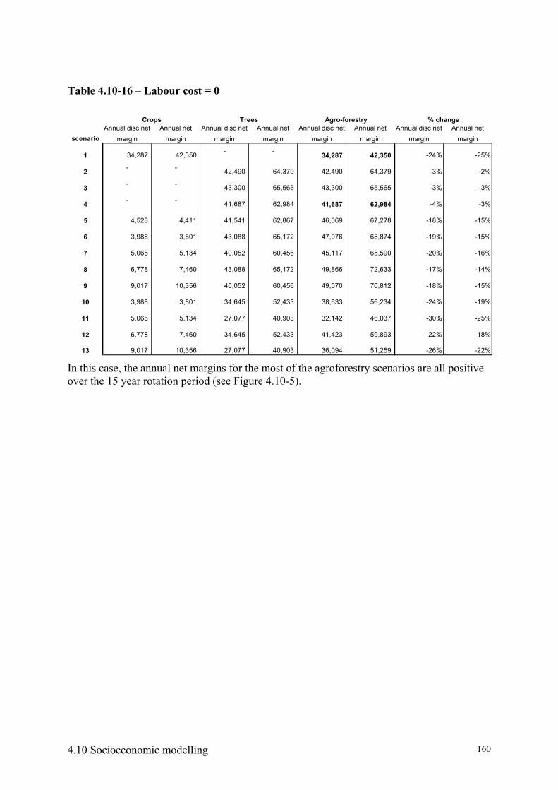
4.10 Socioeconomic modelling 160
Table 4.10-16 – Labour cost = 0
Crops Trees Agro-forestry % change
scenarioAnnual disc net
marginAnnual net
marginAnnual disc net
marginAnnual net
marginAnnual disc net
marginAnnual net
marginAnnual disc net
marginAnnual net
margin
1 34,287 42,350 - - 34,287 42,350 -24% -25%
2 - - 42,490 64,379 42,490 64,379 -3% -2%
3 - - 43,300 65,565 43,300 65,565 -3% -3%
4 - - 41,687 62,984 41,687 62,984 -4% -3%
5 4,528 4,411 41,541 62,867 46,069 67,278 -18% -15%
6 3,988 3,801 43,088 65,172 47,076 68,874 -19% -15%
7 5,065 5,134 40,052 60,456 45,117 65,590 -20% -16%
8 6,778 7,460 43,088 65,172 49,866 72,633 -17% -14%
9 9,017 10,356 40,052 60,456 49,070 70,812 -18% -15%
10 3,988 3,801 34,645 52,433 38,633 56,234 -24% -19%
11 5,065 5,134 27,077 40,903 32,142 46,037 -30% -25%
12 6,778 7,460 34,645 52,433 41,423 59,893 -22% -18%
13 9,017 10,356 27,077 40,903 36,094 51,259 -26% -22% In this case, the annual net margins for the most of the agroforestry scenarios are all positive over the 15 year rotation period (see Figure 4.10-5).

4.10 Socioeconomic modelling 161
Figure 4.10-5 – Annual net margins with zero labour opportunity costs (scenario 13)
Farm Net Margins over 15 years
-5,000
-
5,000
10,000
15,000
20,000
25,000
30,000
1 2 3 4 5 6 7 8 9 10 11 12 13 14 15
Arable margins Forestry margins Agroforestry margins
Discounting rate changes Increasing the discount rate from 3 to 15%, reduces the annual discounted net margin of the arable system from KSh 27,540 to KSh 14,468 (a reduction of 47%). By contrast the reduction in the annual discounted net margins of the forestry system (scenario 2) from KSh 41,404 to KSh 8,175 is equivalent to an 80% reduction. The effect of a high discount rate is more pronounced in systems such as forestry where much of the revenue is obtained towards the end of the rotation period, than in arable systems where the revenue is generally consistent throughout the rotation period. The effect of a higher discounting rate is graphically visible by comparing Figure 4.10-6 with Figure 4.10-3. In the former, the tails of the curves are almost flat.
So with a high discounting rate, forestry and agroforestry scenarios become a much less attractive option for farmers. The possible solution is to shorten the rotation or to select trees with a shorter optimal rotation.

4.10 Socioeconomic modelling 162
Table 4.10-17 – Discounting rate at 15% Crops Trees Agro-forestry % change
scenarioAnnual disc net
marginAnnual net
marginAnnual disc net
marginAnnual net
marginAnnual disc net
marginAnnual net
marginAnnual disc net
marginAnnual net
margin
1 14,468 33,876 - - 14,468 33,876 47% 0%
2 - - 8,175 63,072 8,175 63,072 80% 0%
3 - - 8,187 63,804 8,187 63,804 80% 0%
4 - - 7,951 61,223 7,951 61,223 80% 0%
5 903 - 3,216 8,389 61,861 9,292 58,645 76% 0%
6 558 - 3,826 8,556 63,712 9,114 59,886 77% 0%
7 1,075 - 2,493 8,003 58,996 9,078 56,503 76% 0%
8 1,623 - 167 8,556 63,712 10,179 63,545 76% 0%
9 2,550 2,729 8,003 58,996 10,553 61,725 75% 0%
10 558 - 3,826 6,728 50,973 7,286 47,147 77% 0%
11 1,075 - 2,493 5,175 39,443 6,249 36,950 75% 0%
12 1,623 - 167 6,728 50,973 8,351 50,806 75% 0%
13 2,550 2,729 5,175 39,443 7,724 42,172 73% 0%
Figure 4.10-6 - The net discounting margins with 90% pruning (scenario 7) when discounting rate is 15%
Farm Net Discounted Margins over 15 years
-10,000
-5,000
-
5,000
10,000
15,000
20,000
1 2 3 4 5 6 7 8 9 10 11 12 13 14 15
Arable disc margins Forestry disc margins Agroforestry disc margins

4.10 Socioeconomic modelling 163
4.10.6 Conclusions In a country where pressure on land and agricultural products is constantly increasing and where the majority of the population relies on the outcomes of their own production for survival, consistent and good productivity of farming systems are essential. As land is a scarce resource and the area of land per household is reducing over time, farmers have to maximise the outcome they can get from each hectare.
In this case farmers are faced with two types of trade-off: 1) they have to decide if it is better for them to plant trees or crops, or a combination of them; and then 2) they have to decide which type of tree to plant.
From the surveys in Siaya and Kibwezi it emerged that the majority of farmers accepted a certain level of trade off between crop and trees. They realised that they cannot rely only on crop yield, particularly in Kibwezi where the risk of crop failure is high.
Agroforestry systems provide more financial security to farmers than pure arable and forestry systems because they can spread their investments in the short term in the form of crop yield and in the long term in the form of tree harvest. However, for the agroforestry system to be attractive to subsistence farmers it has to be not only more profitable than the arable system but also to be able to ensure food security.
The economic model simulations showed that
• If we had to choose the scenario solely on the ground of profitability we would choose the forestry system with crown pruning at 50%. In this case farmers will earn most of their income on the last year of the rotation period. However, for subsistence farmers this is an unsustainable option as they would need either access to credits or other sources of income to be able to support themselves during the rotation period. As this is not the case for most of the subsistence farmers in Kenya, this option has to be disregarded.
• Although the agroforestry scenario with 90% pruning provides the lowest returns with respect the other agroforestry and forestry scenarios, it is an attractive option for subsistence farmers since it reduces the years the farmers are in deficit before the trees are harvested, and the returns over the 15 year rotation are higher than the arable system. However, even in the best scenarios with a higher response of crops to pruning the returns from crop production were negative for the last few years.
• When crop prices are unstable, agroforestry systems provide better financial security to the farmer.
• From the analysis of tree price changes, it is clear that farmers should select trees with the highest value, but they should also diversify the type of trees so that a reduction in value in one tree is compensated by the value of another tree. So there should be diversification not only between crops and trees but also between trees. It is important to advocate tree diversity on crop land to reduce the losses if the tree price collapses. In fact if only one species of tree is grown, there is a high probability that during a drought when everyone begins to sell their trees on the local market, this quickly becomes saturated and prices fall. The option of transporting trees outside the affected area could be too costly for farmers themselves. Actions which increase the value of

4.10 Socioeconomic modelling 164
timber products to the farmer, e.g. community-operated portable saw mills, could also be an effective way of increasing the value of tree products.
• Forestry and agroforestry systems become a much less attractive option for farmers when the discounting rate is high. The possible option in this case would be to shorten the rotation or to select trees with a shorter optimal rotation, but this would depend on whether they became more competitive, and their value.
In our case we have run HyPAR simulations assuming a high tree density (179 trees ha-1) when probably a more sustainable option would be to have a lower number of trees per hectare to ensure a higher crop yields. Severe pruning should be a common practice to reduce crop-tree competition and provide an additional source of income in the form of pruning returns.
Although we did not simulate the root pruning, it is clear that such a practice would integrate easily in the farming routine. Farmers do not need to have special plans for root pruning; they can do it when they prepare their land for planting crops (Tefera 2002). When done correctly it is very quick. As it is easily done by women, it potentially draws on a wider labour pool than crown pruning and there will be less requirement for hire of labour.
From the field experiments, no trees died from root pruning and even if the tree standing volume reduced as in scenario 13, the agroforestry option would be still a more profitable option than the arable one with the advantage of reducing the years the farmers is in deficit with respect to the other farming systems. Overall the marginal additional costs spent root pruning would be lower than the benefits from a higher crop yield.
Once farmers decide to plant trees, they must decide which tree to plant. The choice is made not only on the basis of the revenue that they could get from harvesting them in few years time, but also in terms of food security and a source of constant returns. It should be noted that if decisions are taken to plant fruit trees, these will require different management requirements, as crown pruning will reduce fruiting (not tested in this project). However, root pruning may be beneficial to fruiting.
The results of the surveys showed that there was a difference between the Kibwezi and Siaya answers in deciding which tree to plant. In Kibwezi, farmers select the trees that provide them with continuous returns in the form not only of fuel and shade but in particular of fruits, rather than trees that have long-term returns in the form of pole and timber.
Instead when farmers grow timber trees they can see a twofold advantage in pruning. Not only do they reduce the tree competition with crops but also they obtain firewood and actually a better timber bole.
The main problem for subsistence farmers is that they do not have enough savings and access to a cash economy to wait for the revenues from timber in few years time; the risk is too high for them. The risk is highest on small farms. A possible solution is for farmers to locate fruit trees more on the compound and in the grazing land, and fuel wood and pole/timber trees on the cropland, since the pruning of these trees to reduce shading and returns from these trees (clear bole, fuelwood….) are complementary. However, this will be possible only to a certain extent, depending on the compound size and shading properties of fruit trees. High value trees are often planted close to compounds because of the risks of theft and damage by grazing animals on unsupervised plots.

4.10 Socioeconomic modelling 165
It is important to point out that the results of the economic models have to be interpreted as indicative of the dynamics existing between the three farming systems and not to be interpreted literally in terms of magnitude. More simulations should be done by considering different tree density and including root pruning.
References 1. Central Bureau of Statistics, Kenya facts and figures 2002, Nairobi, Kenya. 2. CIA (http://www.cia.gov/cia/publications/factbook/geos/ke.html) 2003
3. David S. and Raussen T (2003), “The agronomic and economic potential of tree fallows on scoured terrace benches in the humid highlands of Southwestern Uganda”, Agriculture Ecosystems & Environment.
4. Dosman D. and Luckert M.K. (1998), “A Micro-economic Primer for Agroforestry related issues in Developing Countries”, IES Special Report No 6.
5. Kiptot E. (2002) personal communication. 6. Kurtz, W.B., Garrett H.E. and Slusher J.P. (2003) “Economics of Agroforestry”,
University Extension, university of Missouri-Colombia.
7. ISS (http://www.iss.co.za/AF/profiles/Kenya/kenya1.html) 2003
8. Morse, K. (1996), “A review of soil and water management research in semi-arid of southern and eastern Africa”. Chatham, UK: Natural Research Institute (NRI)
9. Mulatya J., (2000) “Tree root development and interactions in drylands: focusing on Melia volkensii with socio-economic evaluations, PhD Thesis. University of Dundee.
10. Parry M. L., Carter T.R. and Konijn N.T. (1988) The impact of climatic variations on agriculture, volume 2: assessments in semi-arid regions, Kluwer Academic Publishers
11. Report of 1998/99 Labour force survey in Kenya, Executive summary. 2003
12. Tefera Almaz T., Ong C., Wilson J. and Mugasha A.G., (2002) “Crown and root pruning of four year old boundary trees and their growth at Siaya, western Kenya”.
13. van Keulen Herman, Arie Kuyvenhover and Ruerd Ruben (1998). “Sustainable Land Use and food Security in Developing Countries: DLV’s Approach to Policy Support”, Agricultural Systems, Vol. 58, No. 3.
14. Unicef (http://www.unicef.org/infobycountry/kenyastatistics.html#1) 2003
15. Welfare Monitoring Survey, Central Bureau of Statistics, Kenya 1993.
16. Wilson J. 2003 (Personal communication)

4.10 Socioeconomic modelling 166
4.10.7 Appendices
APPENDIX A - Prices (maize, trees) Tree prices The average price per rotation year20 (column 3 in Table 4.10-18) have been converted to price per volume (column 4 in Table 4.10-18) assuming that the volume obtained from HyPAR simulation (second column in Table 4.10-18) are the average standard tree volume. The tree prices used in the economic model have been obtained by multiplying the tree volume in column 2 with the price per volume for year 15 in column 4 (2560). Figure 4.10-2 uses the price in columns 3 (“Melia jk”) and 5 (“Melia pr (m3)”).
Table 4.10-18 – Tree prices and volume over the 15 year rotation period
year m3/tree KSh/tree KSh/m3 KSh/tree 1 0.00 0 0 2 2 0.00 5 2759 5 3 0.01 28 4887 15 4 0.02 110 5252 54 5 0.07 380 5343 182 6 0.22 650 3005 554 7 0.41 870 2124 1049 8 0.56 1100 1948 1445 9 0.70 1500 2137 1797
10 0.84 1800 2133 2160 11 0.96 2100 2182 2463 12 1.06 2500 2355 2718 13 1.17 2800 2393 2995 14 1.26 3100 2461 3224 15 1.37 3500 2560 3500
Crop prices The maize price is set in Mulatya (2000) at 18 KSh/kg. This price has been used in the combination “maize”; this assumes the same price for both the early and late season crop. The average monthly maize prices for a bag of 90 kg are listed in column 2 of Table 4.10-19 (Source: Kiptot 2002). The average price over a year was calculated (11.6 KSh/kg) and used in the combination “maize pr av”; this combination assumes the same price for both the early and late season crops. As the early harvest is carried out between Jun and July, the maize price for the early crop was set at 7.5 KSh/kg (the average of June and July prices). The late harvest is carried out mainly between November and January, so the maize price for the late crop was set at 18.9 KSh/kg (the average of November and January prices). The combinations “maize pr ses” assumes these two prices.
20 Source: Mulatya 2000

4.10 Socioeconomic modelling 167
Table 4.10-19 - Average monthly maize prices.
month Price (KSh) KSh/kg
Jan 1700 18.9 Feb 1500 16.7 Mar 600 6.7 Apr 500 5.6 May 600 6.7 Jun 650 7.2 Jul 700 7.8 Aug 700 7.8 Sep 1100 12.2 Oct 1300 14.4 Nov 1500 16.7 Dec 1700 18.9
Average 1045.8 11.6

4.10 Socioeconomic modelling 168
APPENDIX B – Discounting The discounted value (or present value) of A KSh that I will gain in t years from now is:
trAPV
)1( += (B.1)
Where r is the discounting factor, often equal to the interest rate.. The formula (B.1) tells us how much the amount A earned in a specific year is “worth” today. For example, KSh 2000 paid in 3 years is worth KSh 1504 today, when the discounting factor is 10%. In fact, I could obtain KSh 2000 in three years times by putting KSh 1504 in a bank and earning 10% per year. Therefore if r increases the present value reduces. In other words, I need to put an amount less than KSh 1504 in the bank, to still obtain KSh 2000 in 3 years. This implies that as r increases more depreciation of natural resources will occur. This is because it is more convenient to harvest, for example a forest, now and put the money earned selling the yield in a bank, rather than leaving the wood to grow more. The concept of discounting is used as the fundamental basis for the CBA (Cost-Benefits Analysis) and CE (Cost-Effectiveness) techniques. Discounting is used to compare combinations of costs and benefits occurring at times in the future. The future streams of costs and benefits are discounted to the present:
∑= +
=T
tt
t
rB
BPV0 )1(
)( and ∑= +
=T
tt
t
rC
CPV0 )1(
)(
Where Bt is the benefit occurring in the year t; and Ct is the cost occurring in the year t. In this way costs and benefits occurring further into the future are given less weight than those that are currently occurring (see Figure 6 page 161). As the discount rate increases the greater is the weight given to costs and benefits occurring in the near future. As the discount rate reduces the greater is the weight given to costs and benefits occurring in the distant future. In CBA analysts evaluate which project to choose using the net present value (NPV) criterion. By definition, the NPV of a project is equal to the present value of the benefits minus the present value of the costs:
∑∑== +
−+
=T
tt
tT
tt
t
rC
rB
NPV00 )1()1(
(B.2)
APPENDIX C - Analysis of survey carried out in Siaya and Embu
Introduction The survey was carried out in 1999. 33 farmers were interviewed in Siaya and Embu. The scope of the survey was to obtain data on the type of trees that were grown on crop land and to assess whether and how pruning was carried out by farmers in these areas. Some comparison with Kibwezi was carried out.
Analysis of survey answers The majority of farmers in Siaya and Embu (97%) own their land. On average farmers hold 4.9 acres of land, in Siaya farmers hold slightly less (4.2 acres) than in Embu (6.8 acres).
The majority of farmers (97%) have trees adjacent to crops. The trees that are more often adjacent to crops are timber trees such as Grevillea and Markhamia (see Table 4.10-20), in

4.10 Socioeconomic modelling 169
Siaya the tree that is most frequently found next to crop is Markhamia. Kibwezi farmers had far more fruit trees planted with crops than farmers at Siaya and Embu. This may relect climatic and economic differences, or differences in opportunity to obtain species at the different sites. The low rainfall at Kibwezi increases the risk of crop failure. Table 4.10-20 Trees adjacent to crops
Frequency Percent Grevillea 12 35% Markhamia 14 41% Eucalyptus 1 3% Fruit trees 1 3% All 5 15% No trees adjacent to crops 1 3% Total 34 100%
Maize was the crop most often grown next to trees. In Siaya almost all farmers plant only maize next to trees (Table 4.10-21). The same is true for Kibwezi, even though this area is generally more suited to grow crops such as millet and sorghum (Parry 1988). Table 4.10-21– Preferred crops with trees
Frequency Percent Maize 19 57% Maize and beans 12 35% Don’t mind, any crop 3 9% Total 34 100%
Farmers recognise that there is competition between trees and crop, as 71% of them stated that crop yield within 2m of trees is a lot less than elsewhere (Table 4.10-22), and 73.5% of farmers described trees next to crops as being heavily shading.. Table 4.10-22 – Yield of crops within 2m of the trees
Frequency Percent About the same as in other plots 7 20% A lot less than in other plots 24 71% Can’t tell 3 9% Total 34 100%
All farmers that were aware of competition between trees and crop either prune or pollard their trees. However only one farmer stated that he prunes all species of trees including fruit trees. The rest of the farmers prune only species of trees that are for timber and poles. In fact the main reason for pruning is not only to reduce shade, but also to get good quality pole/timber and firewood/construction poles; few farmers stated that they were pruning only to reduce shade (Table 4.10-23). Table 4.10-23 – Reasons for pruning
Frequency Percent Reduce shading 4 12% Get firewood/construction poles 2 6%

4.10 Socioeconomic modelling 170
Get quality pole/timber 3 9% All (the reasons above) 25 73% Total 34 100%
Of farmers who gave reasons for not pruning, most of them knew that pruning would reduce fruit production (Table 4.10-24); and17% cited labour shortages. However, many farmers gave no reasons why trees should not be pruned (Table 4.2-7) Table 4.10-24 – Reasons for not pruning
Frequency Percent Get more fruits 16 70% Shade 1 4% More protection against encroachment 2 9% No time or labour to prune 4 17% Total 23 100%
Hire of labour for pruning was more common at Siaya than Kibwezi (Table 4.2-10) On average farmers at Siaya paid KSh 25 per each tree pruned, KSh 20 less than in the Kibwezi area. Tree pruning at Siaya usually took less than thirty minutes. Most of the farmers (60%) pruned trees once a year, and at Siaya, most farmers (85%) used a ladder to climb big trees. Pangas are the most common (88%) tool used for pruning. Men and boys are the ones mainly (80%) responsible to prune trees. Women traditionally are not expected to be responsible to prune trees, if women prune, they only prune young trees. 50% of farmers used prunings only for fuelwood, 22% used prunings both for fuelwood and timber/poles, and 28% of farmers also sold prunings. The average sale price of a bundle of firewood was KSh 28. Most of the farmers that sell their pruning do not need to go to the local market, as buyers came to them. The cash from the sale is used for household needs. The survey carried out in Siaya and Embu was a much shorter version than the one carried out in Kibwezi. For example, in Siaya farmers were not asked what was their main source of income. As the findings from the Kibwezi survey about the difference existing between farmers with off-farm and on-farm income in their decision to plant trees are quite interesting, it is worthwhile to expand a bit on them. In Kibwezi farmers whose income is mainly from on-farm have twice as many natural trees on their farm than farmers whose income source is from off-farm (Table 4.10-25), and farmers whose income is from off-farm plant almost twice as many trees. This is true across all different type of farmers’ land: compound, grazing land and cropland. Farmers with off-farm income seem to be more actively selecting the type of trees they want on their farm by planting them. As farmers with off-farm income have easier access to the cash economy, they can probably buy more easily small tree plants.

4.10 Socioeconomic modelling 171
Table 4.10-25 Income source and frequency of planted and natural trees
Total farm Natural trees Planted trees on-farm off-farm on-farm off-farm Average 101 49 48 85StDev 238 71 59 75Min 0 7 2 1Max 1356 232 271 204Mode 27 13 14 Median 34.5 17.5 20.5 70N. zero 1 0 0 0 Farmers with off-farm income risk less by planting trees on their cropland, the higher risk of crop failure due to competition between trees and crop is not so devastating for this type of household because their main source of income is from off farm. So even if they lose crop yield they are still able to buy food on the local market. Farmers whose source of income is only from on-farm use trees for more purposes than the farmers whose source of income is from off farm. They try to get the most they can from each tree, so they will select those trees that can provide more than one service.

4.10 Socioeconomic modelling 172
APPENDIX D - Welfare tables about Siaya Table 4.10-26 – Mean monthly wage income of household head by socio-economic group (KSh/month) Socio-economic group Own Public
Sector Private Sector
Employer Other All categories
Export farmer-male headed 5,994 11,887 7,165 3,469 2,262 6,272
Export farmer-female headed 3,613 4,300 3,456 12,563 8,579 4,287
Food crop farmer-male headed 4,421 13,420 7,442 1,919 4,839 5,042
Food crop farmer-female headed 3,528 3,297 4,860 1,103 20,154 4,525
Subsistence farmer-male headed 4,957 4,658 3,096 1,223 2,027 4,457
Subsistence farmer-female headed 6,132 10,873 9,185 - 5,328 6,196
Pastoralist 7,385 5,044 17,889 7,597 13,803 8,676 Public sector urban 19,140 12,294 14,104 6,338 7,188 12,917 Public sector rural 3,473 8,229 13,854 6,414 3,723 8,808 Formal sector urban 22,236 18,996 14,643 28,482 21,924 16,015 Formal sector rural 17,728 9,603 8,609 10,231 9,497 10,290 Informal sector urban 37,004 8,532 11,032 14,274 9,832 21,059 Informal sector rural 7,930 8,233 4,542 13,596 5,430 6,813 Income from other sources 6,020 4,836 8,708 2,339 2,544 5,958
Welfare Monitoring survey, Centre Bureau of Statistics, 1993. (Prices inflated to year 2002)
Table 4.10-27 – Mean monthly wage income of household head by region and district Region/district Own Public
Sector Private Sector
Employer Other
All household 8,004 10,074 9,893 10,381 6,325 Rurak 5,772 8,829 6,855 8,115 5,297 Eastern rural 6,866 8,723 4,192 2,780 4,270 Embu 4,186 5,044 2,905 5,301 1,942 Kitui 5,443 4,336 3,473 3,863 16,814 Machakos, Makweni 9,944 13,769 5,922 4,595 7,913 Siaya 3,846 7,750 4,514 848 2,706 Welfare Monitoring survey, Centre Bureau of Statistics, 1993. (Prices inflated to year 2002)

4.10 Socioeconomic modelling 173
Table 4.10-28 – Mean share of household income by source of income and by socio-economic group Socio-economic group Export
crops Food crop sold
Livestock sold
Food crop consumed
Livestock consumed
Wage employment
Self employment
Cash transfers
Remits Other sources
Total income
Export farmer-male headed 26 7 13 17 1 13 14 2 1 3 100 Export farmer-female headed 27 6 16 19 2 8 9 7 1 5 100 Food crop farmer-male headed 29 39 17 2 3 5 3 0 3 100 Food crop farmer-female headed 22 43 18 2 1 3 7 0 3 100 Subsistence farmer-male headed 11 7 64 5 2 3 5 0 3 100 Subsistence farmer-female headed 10 6 64 4 1 2 10 0 3 100 Pastoralist 1 3 50 6 11 3 19 3 2 4 100 Public sector urban 0 0 0 0 85 10 1 2 2 100 Public sector rural 3 5 5 1 77 7 1 1 1 100 Formal sector urban 0 0 1 0 83 13 1 1 1 100 Formal sector rural 2 4 4 0 72 15 1 1 1 100 Informal sector urban 0 0 0 0 54 43 1 1 1 100 Informal sector rural 3 5 7 1 36 44 3 1 2 100 Income from other sources 4 8 15 3 3 5 31 9 22 100 Welfare Monitoring survey, Centre Bureau of Statistics, 1993.
Table 4.10-29 – Mean share of household income by source of income and by region/district Region/district Export
crops Food crop sold
Livestock sold
Food crop consumed
Livestock consumed
Wage employment
Self employment
Cash transfers
Remits Other sources
Total income
All household 4 8 12 17 2 29 16 6 1 4 100 Rurak 6 10 15 21 2 19 18 7 1 5 100 Eastern rural 100 Embu 9 4 16 30 3 15 6 9 1 7 100 Kitui 0 6 27 17 3 29 14 8 0 5 100 Machakos, Makweni 4 5 14 21 2 25 19 6 1 3 100 Siaya 0 8 10 37 2 4 24 10 2 3 100 Welfare Monitoring survey, Centre Bureau of Statistics, 1993.

4.10 Socioeconomic modelling 174
Table 4.10-30 - Percent share of household expenditures by type of expenditure and by socio-economic group (percentage) Socio-economic group Food Own
produced consumption
Basic education
Higher education
Health Non-food Non-consumption
Total Expenditure
Export farmer-male headed 37 17 4 5 2 31 4 100 Export farmer-female headed 41 16 3 5 2 29 5 100 Food crop farmer-male headed 37 18 4 4 2 31 4 100 Food crop farmer-female headed 41 17 4 5 2 26 5 100 Subsistence farmer-male headed 38 29 3 2 1 24 3 100 Subsistence farmer-female headed 38 33 2 3 1 20 3 100 Pastoralist 47 11 3 2 2 28 7 100 Public sector urban 41 0 3 4 1 45 6 100 Public sector rural 37 7 4 6 1 40 6 100 Formal sector urban 38 1 3 3 1 49 6 100 Formal sector rural 44 6 4 5 1 35 5 100 Informal sector urban 44 0 2 2 2 47 4 100 Informal sector rural 49 9 3 2 1 32 4 100 Income from other sources 50 8 3 4 1 30 4 100 Welfare Monitoring survey, Centre Bureau of Statistics, 1993.
Table 4.10-31 - Percent share of household expenditures by type of expenditure and by region/district (percentage) Region/district Food Own
produced consumption
Basic education
Higher education
Health Non-food Non-consumption
Total Expenditure
All household 42 12 3 4 1 33 5 100 Rural 42 15 3 4 1 20 4 100 Eastern rural 45 17 3 4 1 28 4 100 Embu 44 20 3 3 1 24 4 100 Kitui 51 8 4 4 1 29 2 100 Machakos, Makweni 52 14 3 5 1 22 4 100 Siaya 41 28 1 2 2 23 4 100 Welfare Monitoring survey, Centre Bureau of Statistics, 1993.

4.10 Socioeconomic modelling 175
Table 4.10-32 – Percent share of annual household food expenditures by type of expenditure and by socio-economic group (%)
Socio-economic group Own
produced food
Maize Cereal Vegetable Meat Dairy Sugar Oil & fats Roots Other foods
Total food
Export farmer-male headed 30 15 7 6 12 5 13 7 2 2 100 Export farmer-female headed 27 18 7 6 10 5 14 9 1 1 100 Food crop farmer-male headed 32 13 5 6 12 4 17 8 1 1 100 Food crop farmer-female headed 30 15 7 6 10 5 16 8 2 1 100 Subsistence farmer-male headed 41 15 4 5 10 5 12 6 1 1 100 Subsistence farmer-female headed 45 13 6 5 9 5 10 5 1 1 100 Pastoralist 19 25 5 8 8 3 21 8 2 1 100 Public sector urban 1 19 9 13 17 13 10 8 3 6 100 Public sector rural 16 16 7 9 16 8 15 8 2 3 100 Formal sector urban 1 20 8 14 18 13 10 8 2 5 100 Formal sector rural 13 19 8 9 13 10 14 10 1 3 100 Informal sector urban 1 18 10 13 18 14 10 7 3 6 100 Informal sector rural 16 21 7 10 12 8 15 8 2 2 100 Income from other sources 11 22 8 9 13 8 16 9 2 2 100 Welfare Monitoring survey, Centre Bureau of Statistics, 1993.
Table 4.10-33 – Percent share of annual household food expenditures by type of expenditure and by region/district (%) Region/district Own
produced food
Maize Cereal Vegetable Meat Dairy Sugar Oil & fats Roots Other foods
Total food
All household 21 18 7 8 13 8 14 8 2 2 100 Rural 26 17 6 7 12 6 16 8 2 2 100 Eastern rural 27 22 9 9 13 5 15 6 1 2 100 Embu 30 21 6 11 4 7 12 6 1 1 100 Kitui 12 28 9 18 7 4 14 7 1 1 100 Machakos, Makweni 21 24 12 10 7 7 10 6 1 1 100 Siaya 37 15 6 4 14 3 13 6 1 1 100 Welfare Monitoring survey, Centre Bureau of Statistics, 1993.

4.11 Biophysical assessment 176
4.11 A biophysical assessment of the situations in which pruning is likely to be effective and the circumstances for adoption
Within the current project, the pruning of trees was shown to improve crop yield under a variety of circumstances: research station studies at Siaya (sub humid, 1200 mm bimodal), Kifu 1 and Kifu 2 (sub humid, 1400mm bimodal) and Nyabeda (sub humid, 1800 mm bimodal) all showed beneficial effects of trees on crop growth, as did on-farm studies at Kabale (cool highlands with 1200 mm rainfall) and Kibwezi (hot, semi-arid with 500 mm rainfall bimodal). Studies elsewhere also show effectiveness across a range of environments, from monsoonal Bangladesh (Hocking and Islam 1997) to Australian sites with Mediterranean climate and 525 mm unimodal rainfall (Sudmeyer et al. 2002) and sites in Nebraska with 750 mm annual rainfal (Hou et al., 2003). Studies at Kifu 1 (4.4.2) indicated that the increase in crop yield was proportional to the extent of canopy pruning, and studies at Kifu 2 (4.4.3) highlighted the risks to crop yield of only root pruning on one side of the tree, although similar studies at Nyabeda with higher rainfall and soil water did not reveal such a problem. While root pruning on its own sometimes produced remarkable increases in crop yield, this was not always the case, and crown pruning was a more reliable approach, which in addition produces a direct return for the labour expended (firewood). Combined crown and root pruning, as studied at Siaya, Kabale and Kibwezi, was the most effective treatment, but the increase compared with crown only pruning was quite variable according to site and farmers would need to decide whether the effort was justified. Root pruning reduced tree growth less than crown pruning, and combined pruning produced the greatest reduction in tree dbh. Respondents to our surveys and participants in our workshops indicated that crown pruning was largely a ‘man’s job’, whereas women considered that root pruning could be easily incorporated into their land preparation tasks. Biophysically, pruning was an effective treatment in all these environments. Hence it could be used as a management technique in considerable areas of the tropics (and also temperate zones). In agroforestry systems, we are seeking complementarity between different plant components. Cannell et al., 1998 and Huxley 1999 highlighted the importance of controlling competition between trees and crops in locations with 500 – 1100 mm rainfall, where crop yields are very dependent on season, and we have found clear benefits of pruning within these limits. When rainfall is higher, (1100 – 2000 mm) crops can be expected to do well, but shading may become an issue in limiting the growth of C4 plants such as maize, and at higher rainfall, both trees and crops may be light-limited. Hence crown pruning could be of value in these environments to reduce shade, but the merits of root pruning also should not be ignored, as, while water may appear to be generally plentiful, the timing and distribution of its availability are important. The root systems of developing crops occupy the topmost soil layers where evaporation and drainage occur, even when rainfall is high, local soil moisture deficits may arise in these soil layers, especially when soils are free-draining. Root pruning improves the spatial separation between tree and crop roots in this zone and prevents short term competition even where total rainfall appears adequate. The economic attractiveness to farmers will depend on the size of their landholdings and pressures for production of different commodities, relative values of tree and crop products and availability of labour. It certainly offers a means for farms to be managed flexibly, and farmers should be encouraged to try it. While these studies showed that pruning of a wide

4.11 Biophysical assessment 177
range of tree species was effective, it should be remembered that the studies on older trees showed that survival of some species and with repeated cutting could be poor and further investigations are needed to determine the frequency and period of cutting which is possible without causing tree death.

5. Contribution and promotion of outputs 178
5 Contribution of outputs towards DFID’s developmental goals and promotion of results
This project contributes to Millenium Development Goals 1 and 7. It contributes to eradication of poverty and hunger by providing farmers with simple low cost methods of farm management, which enable them to maintain a balance between perennial and annual components of their systems and it contributes to environmental sustainability by enabling trees to be maintained on farms where they might otherwise be removed.
5.1.1 Promotion strategy for R7342 Stakeholder and process diagram
Research team
Other staff in team’s insitutions
DFID – FRP and local advisers
Other projects in which team members
are involved
Farmers involved in farm and research
station trials
Meetings, leaflets, visits, publications
Stakeholders
Mechanisms
District officers, community groups
etc
Exchange visits, video, workshops, practical
demonstrations, leaflets, posters
Global scientific community
Publications and presentations at
meetings
Wider local community
Visits, video, posters and leaflets
The promotion process has been cautious because the true effects of experimental treatments (eg pruning and repeated pruning impacts on tree growth rates and survival, root pruning

5. Contribution and promotion of outputs 179
impacts on tree stability) can be expected to take some time to manifest themselves. The degree of involvement with the community varied with location and objectives of studies at that location. Details are given below:
Uganda 1. At Kabale, much of the experimentation was on farm and so farmers were directly
involved in the execution and management of the studies. At the same time, there was also close involvement of community groups, especially in the second phase of the project when they set up and ran their own experimental and training areas. On farm trials test the effects of pollarding and combined pollarding and root pruning. Because of fears about the loss of stability resulting from root pruning, most of the direct promotion work (at least in the early stages of the project) focused on the promotion of pollarding rather than root pruning, and farmers were left to judge root pruning for themselves.
There are very good links between the local project managers and community groups in Kabale and the opportunity was taken to build on these and take a small group of community leaders to Embu in Kenya, for them to learn how farmers working in a similar environment cope – learning not only about pruning, but also about all aspects of farm life including diversification of crops, establishment of on-farm nurseries, milk production and biogas production. A video and leaflets / wall planners were produced to use as training tools for a wider pool of farmers. The video was produced in 3 languages: Rukiga for use in SW Uganda, Swahili for use in Kenya and English for general use). The wall planner was produced in Rukiga for local use and English for general use. In the second phase of the project, there was direct involvement of a local CBO, the Ndorwa Agroforestry Association, which set up on farm demonstration plots and nurseries and conducted training in their own communities. Especially in the second phase of the project, there was intensive training, both of local groups and also through visits to individual farmers, using the materials produced. A local drama group developed a theatrical training presentation. In addition, a small booklet was produced, outlining the reasons for tree management. Formal workshops were run at the project planning stage at the start and finish of the contract. Participants were a mix of scientists (project and non-project), policy makers and community groups.
2. Kifu. Studies here were restricted to research station plots where the main focus of the work was in understanding effects of root pruning, therefore promotion was on a much reduced level relative to Kabale. There was no outreach training, but there were several station visits by farmers to see on-site demonstrations and a workshop involving farmers, and local institutions and policy makers.
Kenya 3. Siaya. Studies at Siaya focussed on pruning relatively large trees. Local farmers were
employed and trained to assist with the pruning and much of the site management. Regular site visits were organised with local farmer groups to demonstrate pruning

5. Contribution and promotion of outputs 180
and show the outcomes of it. A workshop was held at the end of the project to which local farmers, representatives of local and national organisations and staff and students of the Siaya Technical Institute which hosted the field study were invited.
4. Kibwezi / Kitui. These sites were added in the second phase of the project. There are
excellent links between project staff and the local community in these areas, through a series of projects. Trials at Kibwezi are on farm and particular farmers are being targeted as ‘farmer trainers’ in the local community, and local community groups (Masocud, Vinya wa ititi). Training materials were produced and disseminated and the video was used in local dissemination sessions.
Broader scientific community The outputs of the project will be promoted through publications in scientific journals and conference presentations where possible. Several publications are in preparation (2 from Kabale, 2 from Kifu and 2 from Kenya). Furthermore, the work is now being followed up through other projects in East and West Africa in which CEH has an involvement. In Kenya, KEFRI are continuing with evaluations of pruning effects in drylands and in Uganda, the work is being promoted by FORRI at both Kifu and Kabale. During this project, scientific and technical staff received a considerable amount of training at a variety of levels. Two PhDs have been awarded (Wajja-Musukwe 2003; Tefera 2004) and field data from the Kabale part of the project was used as the basis of a Master’s thesis (Sande 2002). There has been much additional training, especially in data collection, analysis and evaluation.
Outputs are listed in Annex 2.

6. References 181
6 References Cannell, MGR, van Noordwijk, M, & Ong, CK (1996) The central agroforestry hypothesis: the tree must acquire resources that the crop would not otherwise acquire. Agroforestry Systems 34: 27-31. Carswell G. 2002. Farmers and fallowing: agricultural change in Kigezi District, Uganda. The Geographical Journal 168(2): 130 – 140. Cooper, PJM, Leakey, RRB, Rao, MR & Reynolds, L (1996) Agroforestry and the mitigation of land degradation in the humid and sub-humid tropics of Africa. Exptl. Agric. 32: 235-290. Corlett, JE, Black, CR, Ong, CKand Monteith, JLM. (1992) Above and below-ground interactions in a leucaena/millet alley cropping system.2.Light interception and dry matter production. Agricultural and Forest Meteorology 60: 73-90. Daniel, J.N.,Ong,C.K.and Kumar,M.S. (1991) Growth and resource utilisation of perennial pigeonpea ( Cajanus cajan (L) Millsp) at the tree-crop interface. Agroforestry Systems 16:177-192. David S. and Raussen T. 2003. The agronomic and economic potential of tree fallows on scoured terrace benches in the humid highlands of Southwestern Uganda. Agriculture Ecosystems and Environment 95: 359 – 369. Digby, P., Galwey, N and Lane, P. (1989) Genstat 5 A Second Course. Oxford University Press. 233 pp. George E. 2002. Woodstoves for Uganda: testing stoves and finding better designs. Ministry of Energy and Mineral Development. GTZ. 37 pp. Hocking, D. (1998) Trees in wetland rice fields: a successful tree management technology through participatory action-research in Bangladesh. Agroforestry Today, July – Sept 1998, 4 – 6 Hocking, D, and Islam, K. (1997) Trees on farms in Bangladesh: 5 Growth of top- and root-pruned trees in wetland rice fields and yields of understorey crops. Agroforestry Systems 39: 101 – 115. Hou, Q, Brandle, J, Hubbard K, Schoeneberger, M., Nieto, C., and Francis, C. 2003. Alteration of soil water content consequent to root-pruning at a windbreak/crop interface in Nebraska, USA. Agroforestry Systems 57: 137 – 147. Howard, SB, Ong, CK, Black, CR and Khan, AAH (1997) Using sap flow gauges to quantify water uptake by tree roots from beneath the crop rooting zone in agroforestry systems. Agroforestry Systems 35: 15-29.

6. References 182
Hytonen J. and Issakainen J. 2001. Effect of repeated harvesting on biomass production and sprouting of Betula pubescens. Biomass and Bioenergy 20 (4): 237 – 245. Ingleby, K, Diagne, O, Deans, JD, Lindley, DK, Neyra, M and Ducousso, M (1997) Distribution of roots, arbuscular mycorrhizal colonisation and spores around fast-growing tree species in Senegal. For. Ecol and Manage. 90: 19-27 Jain R.K. and Singh B. 1999. Fuelwood characteristics of selected indigenous tree species from central India. Bioresource Technology 68: 305-308. Jones, M and Sinclair, F (1995) Differences in root system responses of two semi-arid tree species to crown pruning. Agroforestry Forum 7(2): 24-27. Khan, AAH and Ong, CK (1995) A low cost heat pulse method for measuring tree root water uptake. Agroforestry Forum 7(2): 19-21. Korwar, GR and Radder, GD (1994) Influence of root pruning and cutting interval of Leucaena hedgerows on performance of alley cropped rabi sorghum. Agroforestry Systems 25: 95-111. Lott, JE, Khan, AAH, Ong, CK and Black, CR 1996. Sap flow measurements of lateral tree roots in agroforestry systems.Tree Physiology 16: 995-1001. Mulatya, J.M., Wilson, J., Ong, C.K., Deans, J.D., and Sprent, J.I. 2002 Root architecture of provenances, seedlings and cuttings of Melia volkensii: implications for crop yield in dryland agroforestry. Agroforestry Systems 56: 65-72. Odhiambo HO, Ong CK, Wilson J, Deans JD, Broadhead J and Black CR (1999). Tree-crop interactions for below ground resources in dry lands: root structure and function. Annals of Arid Zone 38: 221-237 Odhiambo, H.O., Ong, C.K., Deans J. D., Wilson, J., Khan, A.A.H., and Sprent, J.I. (2001) Roots, soil water and crop yield: tree crop interactions in a semi-arid agroforestry system in Kenya. Plant and Soil 235: 221 – 233. Okorio J (2000). Light interception and water use in boundary planting agroforestry systems. Unpublished PhD thesis, University of Reading, UK. Okorio, J, Byenka, S, Wajja, N and Peden, D (1994) Comparative performance of seventeen upperstorey tree species associated with crops in the highlands of Uganda. Agroforestry Systems 26: 185-203. Ong, CK, Deans, JD, Wilson, J, Mutua, J, Khan, AAH & Lawson, EM (1999) Exploring below-ground complementarity in agroforestry using sapflow and root fractal techniques. Agroforestry Systems.

6. References 183
Ong, CK, Corlett, JE, Singh, RP and Black, CR (1991) Above and below ground interactions in agroforestry systems. For. Ecol. Manage. 45: 45 - 57. Ong, CK and Khan, A.A.H (1993) The direct measurement of water uptake by individual tree roots. Agroforestry Today 5: 2-5. Ong, CK (1995) The 'dark side' of intercropping: manipulation of soil resources. In: Ecophysiology of Tropical Intercropping. Conference Proceedings, Guadeloupe, INRA, France. Ong, C.K., Wilson, J., Deans, J.D., Mulatya, J.M., Raussen, T., and Wajja-Musukwe, N. 2002. Tree-crop interactions: manipulation of water use and root function. Agricultural Water Management 53(1-3) 171-186. Peden, DG, Okorio, J, Wajja-Musukwe, N (1996) Commercial pole production in linear agroforestry systems. Agroforestry Systems 33: 177 – 186 Peden, D.G., Wajja-Musukwe, N., and Okorio J. 1997. Crop and upperstorey tree production in linear agroforestry systems in Uganda. ICRAF AFRENA report no. 116. 28 pp. Schroth, G. (1995) Tree root characteristics as criteria for species selection and system in agroforestry. Agroforestry Systems 30: 125-143. Sims R.E.H., Senelwa K., Maiava T. and Bullock B.T. 1999. Eucalyptus species for biomass energy in New Zealand – Part II: Coppice performance. Biomass and Bioenergy 17(4): 333 – 343. Singh, RP, Ong, CK and Saharan, N (1989) Above and below-ground interactions in alley cropping in semi-arid India. Agroforestry Systems : 259-274. Sudmeyer, RA, Hall, DJM, Eastham, J, Adams, MA 2002. The tree-crop interface: the effects of root pruning in south-western Australia. Australian Journal of Experimental Agriculture 42: 763 – 772. Tyndall, B. 1996 a The anatomy of innovative adoption: The case of successful agroforestry in east Africa. Ph.D Thesis, Colorado State University. Tyndall, B. 1996 b. The socioeconomics of Grevillea robusta within the coffee land-use system of Kenya. AFRENA report, September 1996, 71 pp. van Noordwijk, M, Spek, LY & de Willigen, P (1994) Proximal root diameter as predictor of total root soze for fractal branching methods. Plant and Soil 164: 107 - 117 van Noordwijk, M & Purnomosidhi, P (1995) Root architecture in relation to tree-soil-crop interactions and shoot pruning in agroforestry. Agroforestry Systems 30: 161 - 173.

6. References 184
Wajja-Musukwe, N., Bamwerinde, W., Siriri, D. and Mbalule, M. 1998. Research on upperstorey trees for the Kigezi Highlands. In ‘AFRENA Uganda Project. Progress report September 1996 – December 1997. AFRENA report no. 121, pp. 10 – 16. Wilson, J, Deans, JD, Ong, CK, Khan, AH, Odhiambo, HO (1998) Comparison of tree: intercrop interactions of Gliricidia and Grevillea in semi-arid Kenya. Final Technical Report July 1995 – March 1998. DFID contract no. R6321 Wilson, J., Deans, JD, Wajja-Musukwe, N., Raussen, T., and Ong, CK. (1999) Project Intitiation Workshop – Pruning effects on root function, Kabale, Uganda 19 – 21st January 1999. Yevich R. and Logan J.A. in press. An assessment of biofuel use and burning of agricultural waste in the developing world. Global Biogeochemical Cycles.

Annex 1: research design and data analysis
J. Wilson, CEH Edinburgh
Annex 1: Research design and data analysis
Final Technical Report to DFID
ZF0094 / R7342
Annex 1: research design and data analysis i
1.1 Certification..............................................................................................................ii
1.2 Introduction to Experimental Protocols ................................................................1
A1.1 Experimental protocol no. 1....................................................................................5
A1.2 Experimental protocol no. 2....................................................................................8
A1.3 Experimental protocol no. 3....................................................................................9
A1.4 Experimental Protocol no 4...................................................................................13
A1.5 Experimental Protocol no 5...................................................................................15
A1.6 Experimental Protocol no 6...................................................................................17
A1.7 Experimental Protocol no 7...................................................................................18
A1.8 Survey protocol no 1. To gather baseline information on pruning practices in Kenya and Uganda.................................................................................................................20
A1.9 Survey protocol no 2. To gather baseline information on pruning practices at Kibwezi 28
A1.10 Survey protocol no. 3 .........................................................................................33

Annex 1: research design and data analysis ii
6.1 Certification A letter from Richard Coe, principal biometrician at ICRAF, is attached.

United Nations Avenue, Gigiri | PO Box 30677-00100 Nairobi, Kenya | Ph: 254 20 524236 or via USA 1 650 833 6645 Fax: 254 20 524001 or via USA 1 650 833 6646 | Email:[email protected] | http: www.worldagroforestrycentre.org
iii
05 November 2003 Research Protocols for R 7342 : 'Pruning to improve spatial complementarity in utilization of below ground resources' I have reviewed the protocols for 7 experiments and 3 surveys carried out under this project. The designs and methods described are appropriate for the objectives and are generally efficient ways of generating the required information. They are statistically valid The requirement to have the protocols reviewed by a biometrician was introduced after these studies had been conducted. However I was able to make suggestions on both how the trials were described and on appropriate methods of analysis, both of which have been adopted.
Richard Coe Principal Biometrician and Head, Research Support Unit.

Annex 1: research design and data analysis 1
6.2 Introduction to Experimental Protocols A previous DFID FRP project (R6321) with CEH, ICRAF and others, highlighted the importance of below-ground competition between trees and crops and indicated that the selection of trees with uncompetitive root architecture was unlikely to be an option, because even a few tree roots in the crop rooting zone can be highly competitive. A proposal to FRP was drawn up to test the effects of tree pruning and the project outputs were defined as below (extract from project memorandum).
A start-up workshop was held in Uganda under R7321 to gain views of target institutions and stakeholders. A key output of that workshop was a narrowing of the focus of this project, to concentrate on extreme crown pruning methods and on root pruning, and rejecting less extreme crown pruning methods (Wilson et al., 1999). As a result of that workshop, the project outputs were defined as follows: ‘…..
1. Current farmer pruning practices and factors influencing the use of pruning analysed in 2 communities in Uganda and 2 in Kenya.
This provides the data against which the subsequent impact of the project can be judged, the methodologies currently employed by farmers and the reasons why they currently prune or do not prune.
2. Views of farmer groups and NGOs at an interactive workshop held early in the project on the relevance and applicability of different pruning techniques obtained and the proposal modified.
This output ensures that the proposed activities have the support and meet the needs of farmers and NGOs.
3. Potential of extreme crown pruning of large trees for controlling competition between trees and crops examined and quantified.
4. Potential of early crown pruning of young trees as a means of controlling competition examined and quantified.
5. Potential of root pruning of trees as a means of controlling competition for water and controlling zones of water extraction examined and quantified.
Through these outputs we will increase our understanding of how trees react to pruning, how this impacts on tree and crop productivity and the consequences for soil moisture in and below the crop rooting zone.
6. Potential of severe shoot and root pruning for controlling competition between trees and crops investigated in on-farm trials, with farmer evaluation of pruning effects, and methodologies, consequences and costs. Techniques and information disseminated through ‘farmer days’.
Farmer managed experiments should ensure relevance of approaches, improve dissemination and feedback, and will enable comparison of research station / on farm results. There will be a feedback loop between 3 – 5 and 6 to ensure that research directions meet farmer needs.
7. Dissemination of results of project by pruning bulletins, farmer days, contract reports, scientific papers and final workshop.

Annex 1: research design and data analysis 2
Previous studies at Machakos indicated that some tree species were already highly competitive, 30 months after planting. In order to study the impacts of pruning on reducing competition, within the confines of a 3-year project, it was necessary to identify sites which already had trees of sufficient age to be competitive with crops. At the same time, because trees of different ages and species might be expected to recover differently from pruning it was important to test the methods on as wide a range of species and ages as was practicable. Furthermore, in order to determine the general applicability of the approaches to different climates, it was desirable to conduct studies across a range of sites differing in rainfall. Needless to say, budgetary limitations were also important in selecting the range of sites and activities to be conducted at them. In the first phase of the project, sites were identified as in Error! Reference source not found.. However, Machakos became unavailable due to changes in site management, and planned activities (primarily related to sapflow studies) were relocated to other sites. It was recognised that this removed the driest site from the study, and when the project was extended by a year, the opportunity was taken to introduce drier sites at Kitui and Kibwezi (Error! Reference source not found.). Table A1-1 Research plots in Uganda and Kenya: Phase 1
Country Location Annual rainfall (mm)
Planting date
Design Tree species available for the study
Uganda Kabanyolo1 1400 mm bimodal
1988 randomised complete block design, with crop only control, 3 blocks. Plots are 16 x 6 m, with a single row of trees planted 2 m apart along the long axis.
Alnus acuminata, Casuarina equisetifolia , Maesopsis eminii, Markhamia lutea, Melia azederach, Cupressus lusitanica, Cordia abyssinica
Uganda Kifu 1 1400 mm bimodal
Randomized complete block design, 3 blocks, 3 different pruning intensities (removal of bottom 1/3, 2/3 of canopy and pollarding (whole crown removal), with control
Cordia africana, Grevillea robusta, Senna spectabilis
Uganda Kifu 2 1400 mm bimodal
1995 Randomised block design, with crop only control 25 trees per plot, 4 blocks with a central tree row. Trees currently at 1 m spacing, due to be thinned in 1999.
Alnus acuminata Grevillea robusta, Maesopsis emininii Casuarina equisetifolia, Markhamia lutea
Uganda Bushenyi 1168 mm bimodal
1990 5 – 15% slope Linear planting on contour rows, 3 replicate plots, 5 trees per plot
Acacia melanoxylon, Periserianthes falcataria, Alnus acuminata, Causarina cunninghamiana, Casuarina equisetifolia, Casuarina glauca, Eucalyptus grandis, Grevillea robusta, Maesopsis eminii, Polyscias fulva,Cupressus lusitanica, Cordia abyssinica
Uganda Kalengyere 1082 mm bimodal
1990 10 – 25 % slope Linear planting on contour rows, 3 replicate plots, 5 trees per plot
Acacia melanoxylon, Periserianthes falcataria, Alnus acuminata, Causarina cunninghamiana, Casuarina glauca, Cedrela odorata, Eucalyptus grandis, Grevillea robusta, Polyscias fulva, Melia azederach, Markhamia lutea

Annex 1: research design and data analysis 3
Uganda Kachwekano 988 mm bimodal
1990 25 – 45 % slope Linear planting on contour rows, 3 replicate plots, 5 trees per plot
Acacia melanoxylon, Periserianthes falcataria, Alnus acuminata, Causarina cunninghamiana, Casuarina glauca, Cedrela odorata, Eucalyptus grandis, Grevillea robusta, Polyscias fulva, Markhamia lutea, Maesopsis eminii
Kenya Machakos 740 bimodal 1993 randomised complete block design, with crop only control, 4 blocks. Plots are 18 x 18 m with a central single tree row. Interplot root competition has been prevented by repeated trenching around the plots.
Senna siamea, Melia volkensii, Grevillea robusta, Gliricidia sepium, Casuarina equisetifolia, Croton megalocarpus, Leucauena leucocephala, leucaena collinsii
Kenya Siaya 1 1200 mm bimodal
1995 Randomised design, 5 basal P treatments x 3 reps x 6 tree species. Plots are 7 m long, 4 trees per plot with a central tree row. Intercropped with sorghum. Plots have never been trenched.
Eucalyptus camaldulensis, Alnus acuminata, Cedrela serrata, Markhamia lutea, Casuarina equisetifolia, Grevillea robusta
Kenya Siaya 2 1200 mm bimodal
1997 Randomised block design, 2 basal P treatments, x 4 tree species and crop only control, 4 blocks.
Grevillea robusta, Eucalyptus camaldulensis, Cedrela serrata, Markhamia lutea
Kenya Nyabeda 1800 mm bimodal
Randomised block design, 2 basal P treatments, 4 tree species and crop only control, central tree row, 15 trees per plot.
Grevillea robusta, Eucalyptus camaldulensis, Cedrela serrata, Markhamia lutea
Table A1-2 Additional research plots in Kenya, Phase 2.
Location Annual rainfall (mm)
Design Tree species available for the study
Kitui* 700 mm bimodal
On farm Melia volkensii
Kibwezi 650 mm bimodal
On farm Melia volkensii
Kitui and Kibwezi
On station. Randomised block design, 10 trees per plot.
Acacia polyacantha Grevillea robusta Senna spectabilis Melia azedirach
Recognising the interest raised at the start up workshop in extreme crown pruning techniques led us to adopt variations of the crown pruning method which many farmers use in Embu on boundary trees. In this, most of the side branches are removed every 18 – 24 months and the top is lopped. Many Embu farmers prune the side branches very crudely, missing the opportunity to improve timber quality by reducing knots. Although this side pruning and lopping technique appears very severe – virtually no leaf is left on the tree after pruning and substantial amounts of biomass are removed, the experience of farmers at Embu is that it works and enables them to obtain regular yields of poles and firewood. Many of them are less certain about its role in reducing tree competition with crops. There is very little practice or awareness of root pruning, but studies in Bangladesh (Hocking 1998; Hocking and Islam, 1998) have demonstrated its ability to improve compatibility with crops, even where soil water appears abundant.

Annex 1: research design and data analysis 4
In terms of selection of tree species, it was necessary to work with what was available in sufficient numbers to permit reasonable replication. Because old trials were often used, the species cover those which have previously been considered to be worth testing for the particular locations, and many of them are widely planted by farmers. One species, Grevillea robusta, occurred at most sites, and so observations on this provide a certain amount of insight into whether species’ reponse may vary according to environment. Impacts of crown and root pruning on crop growth are likely to depend upon the extent to which tree presence exacerbates water stress of the crop. The impacts of root pruning may vary according to whether the trees are shallow rooted or not. Current knowledge on this subject is limited and the contribution of species, provenance and site to root architecture is not understood.

Annex 1: research design and data analysis 5
A1.1 Experimental protocol no. 1 Effects of pollarding, side pruning and root pruning on tree growth and crop yield in farmers’ fields in SW Uganda Justification for: Trees planted in small terraced farmers’ fields in SW Uganda reduce crop yield substantially. Pruning may provide a simple method to reduce tree competition and therefore allow farmers to manage their land to obtain a better balance between tree and crop production. Logic supporting: Crop yield is affected by competition for water, light and nutrients. Crown pruning of trees reduces demand for water by reducing transpirational area and reduces shade. Root pruning is expected to displace tree root activity below the main crop rooting zone. Experimental design: For tree growth, 2 tree species and 3 pruning treatments. Tree species: T1 = Alnus acuminata T2 = Grevillea robusta Pruning treatments:P1 = pollarding and side pruning
P2 = pollarding, side pruning and root pruning P3 = no pruning
Farm sites: An on-farm trial, with rows of A. acuminata and G. robusta, previously planted by AFRENA (in 1994) in the Katuna Valley was used (Wajja-Musukwe et al., 1998). In this trial, rows of individual tree species, at 2 m spacing, were planted, with adjacent control, no tree plots. Most of the rows were planted along the lower edges of terraces, a few were planted along the upper edge, and a very few across the middle (when terraces were wide). Utilising this existing on-farm trial meant that we could test out the techniques on two tree species which are being promoted in the area, and engage farmers directly in the process. Eucalyptus is the only other species widely planted in this area, which is already managed in woodlots by coppicing. Neither Alnus nor Grevillea are being managed, apart from some removal of lower branches. Initially, 45 groupings of trees were selected, however some were later removed from the study due to damage by grazing and other difficulties. Ultimately, detailed tree evaluations were conducted with 14 farmers, across 5 subcounties. The trees were located in 19 fields within these farms, in 37 groupings where Alnus and Grevillea were planted along the same row and one group where Alnus was alone. Of the 37 groups, 30 were at the lower edges of terraces (where trees are most commonly planted), 2 were at the upper side of the terrace and the remainder were in intermediate postions. The additional Alnus group was also at the lower side. Pruning treatments: Tree rows typically had 6 – 8 trees of a species. Pruning treatments were applied to pairs of adjacent trees, which were selected at random from within the tree rows.

Annex 1: research design and data analysis 6
P1 was done as follows: The top was removed (pollarding) by a slanting cut. The height of cut was determined in consultation with the farmers. The standard length of timber in Kabale is 4.7 m, so the height of pollarding was usually set at approximately 5m, unless the tree was of sufficient height to enable two lengths to be obtained. At the same time, virtually all the branches were removed, except for a few which were cut back to stumps to allow access for future pruning, and a few stumps just below the lopping point (side pruning).
P2 as P1, with the addition of root pruning on one side of the tree. At 50 cm distance from the
tree row, and on the side of the tree on which crops are planted, a trench 50 cm deep was dug and all the tree roots in the trench were cut, and the trench refilled.
P3 no pruning treatments imposed
Tree assessments Height before pruning was measured, as well as diameter at breast height and root collar diameter. These last two were also measured at intervals during the duration of the experiment. Biomass of prunings, and time taken to prune were also determined as appropriate. Crop evaluations were conducted in 2000 (beans) on 3 lower, 3 upper and 2 intermediate tree positions, with Grevillea and Alnus together at each location. In this season, replication of the treatments was poor and crop growth in the absence of trees was not evaluated. In 2001 (maize), better replication was possible in some locations and 6 lower, 3 upper and 2 intermediate positions were used, all with controls and all with Alnus and Grevillea together. Crop growth and yield were assessed in different rows at different distances away from the trees, which had received the different pruning treatments. Harvesting and sampling was done on an area of 3 m x 1 m (3 m2) for beans and 3 m x 1.5 m (4.5 m2) for maize, i.e. two adjacent crop rows were combined for each harvest. The influence of distance from trees on crop yield was measured from 1 m to 5 m in the first bean season. In the second maize season, harvesting was extended to 8 m away from trees. In each harvesting plot, bean pods were collected and shelled in the field to obtain seeds, and maize cobs were shelled and bean seed and maize grain fresh weights were recorded to the nearest 1 g. Oven dry weights were then obtained by drying subsamples to constant mass at 70oC.
Data analysis
Tree growth Because tree growth data was unbalanced, REML was used in preference to ANOVA to determine the effects of pruning treatments on tree growth. Within Genstat, the repeated measures option was selected and the following options were then set: data in multiple variates; time points evenly spaced. The autoregressive order 1 model was selected in

Annex 1: research design and data analysis 7
preference to the ‘split-plot in time’ option because preliminary ANOV of this data indicated that data from adjacent time points was more closely correlated than data from non-adjacent points. Treatments were set as tree species*pruning. Data will be checked for heterogeneity of variances and transformed if necessary. If transformation is not suitable, consider using glms that do not assume constant variance. The first set of measurements was taken before the treatments are imposed, analysis of these data shows that the sizes of trees allocated to the different treatments were not significantly different.
Crop Yield Nb. Even in the absence of trees, crop growth is not uniform on these fields because they are steeply sloping and the most fertile and deepest soil is at the lower end of the slope. So, when trees are planted at the bottom of the slope, the effect of the tree in reducing crop growth in its proximity, may be counterbalanced by the effects of improved fertility and soil depth in this area. Conversely, when trees are planted at the top of the slope, the effects of competition may exacerbate the effects of poor soil. The effects of location on soil fertility will be apparent from the control plot crop data. Whereas it appears reasonable to analyse effects of pruning on trees without regard to the position of the trees on the terrace, this is not the case for the crop growth, where tree position on terrace effects are likely to be important. Because of the poor replication on the upper and intermediate parts of the slope, the analysis will focus on the lines of trees at the ‘lower’ position. The layout is a split plot for tree species. Yields will be considered at the subplot level and not broken down further to evaluate distance effects, because farmers are interested in total yield, not in the distribution of the yield. Because pruning treatments may have different effects on crop yield according to tree species, the analysis will be set up to compare the different pruning treatments within a tree species against the no tree control. Block = line of trees ( Alnus and Grevillea) in farmers fields, containing P1, P2 and P3 and no tree control (C ) Splitplot = defining the two tree species and control ( = ‘species’) SubPlot = defining the different pruning treatments and the no-tree control ‘treat’ So in Genstat Block Block/splitplot/subplot/ Treat Species*Treat For ANOVA, a probability of 0.05 or less was accepted as indicating that treatment effects were occurring. If significant effect did occur, means were distinguished by Fisher’s Least Significant Difference (LSD).

Annex 1: research design and data analysis 8
A1.2 Experimental protocol no. 2 Impacts of extreme crown pruning of large trees on tree growth, recovery and survival in Uganda Objectives: To determine impacts of severe lopping and side pruning on ‘mature’ trees. This study was intended to be of short duration, extreme pruning treatments would be imposed, survival assessed, and tree species characterised for their size etc. This study utilises trials at Bushenyi, Kalengyere and Kachwekano (SW Uganda) set up in 1990 by AFRENA (Peden et al., 1997), and also a trial set up at Kabanyolo at Makerere University Farm. Bushenyi, Kalengyere and Kachwekano: At each site, rectangular plots consisting of a single contour row of upperstorey trees planted lengthwise along the middle of the plot. Intra-row spacing was 2 m. There were five trees per plot, excluding two guard trees. Plots were laid out in a completely randomised design with 3 replications. Peden et al., 1977 observed growth and biomass production for 41 months. During this time, trees were managed by side pruning the lower third. In 1994, the central 5 trees in each plot at each site were cut for determination of growth and biomass. In our study, all seven trees on the plot were measured, pollarded and side pruned, thus obtaining an estimate of the response to severe pruning when there had been no previous history of significant pruning, and also when the trees had been previously coppiced. At start of our measurements, trees were thinned to one coppice stem and the growth of this one was followed. Trees 1 and 7 had never been cut before, the rest had been coppiced by Peden. After the thinning was done, the thinnings were weighed and then the remaining shoot was pollarded and the prunings weighed. Then regrowth of the single remaining stem was measured. Kabanyolo: This trial was planted in 1988, 3 blocks, 7 tree species in plots with (usually) 5 trees per plot. Trees were pollarded at 5 m and side pruned in 1999. Biomass offtake, tree size and tree recovery were recorded. Data analysis: Because of the mixed history of the site, only simple analysis is appropriate, or necessary. % survival of species (and tree size) and biomass offtake will be calculated.

Annex 1: research design and data analysis 9
A1.3 Experimental protocol no. 3 Effects of root pruning on tree growth, crop yield and soil water at Kifu, Uganda. Tree species: Grevillea robusta, Casuarina equisetifolia, Maesopsis eminii, Markhamia lutea and Alnus acuminata Justification for: Evidence from Okorio (2000) indicates that crop yield at this research station site is substantially reduced close to trees. Although his data implicates shading as the causal factor, there is reasonable preliminary evidence from Machakos (Odhiambo et al., 1999, 2001) to indicate the importance of below ground competition. This study evaluates the effect of root pruning on one side of trees only on crop and tree growth. Logic supporting: Crop yield is affected by competition for water, light and nutrients. Root pruning is expected to displace tree root activity below the main crop rooting zone, or, as these trees are pruned on one side only, increase root activity on the unpruned side. Experimental design: Five tree species and crop only control and 3 pruning treatments Tree species: T1 = Grevillea robusta T2 = Casuarina equisetifolia T3 = Maesopsis eminii T4 = Markhamia lutea T5 = Alnus acuminata T6 = crop only Pruning treatments: For analysis, the pruning treatments need to be considered in different ways, depending on whether it is tree growth that is being assessed, or whether it is crop growth, root growth and soil water. For tree growth TP1 = root pruned one side TP2 = not root pruned For crop growth, root growth and soil water
P1 = root pruned plot, the side of the tree where root pruning was done P2 = unpruned plot (measured on the same side of the tree row as P3) P3 = root pruned plot, the side of the tree where root pruning was not done.
Site At FORRI’s Kifu Research Station (0° 48´ N, 32° 46´W, 1250 m a.s.l.) Mukono district, central Uganda. Using a pre-existing trial (Okorio 2000) which was planted in September 1995. A row of seedlings at 1 m spacing was planted along the central short axis of each 25 x 30 m plot. In 1998, alternate trees were removed, so that there was 2 m between trees at the time of this study, which commenced in 1999.

Annex 1: research design and data analysis 10
There were 4 blocks. Root pruning was done by digging a trench 30 cm deep by 30 cm wide on one side of the tree line, 30 cm away from the base of the tree. This was done on one side of the tree row, on half the length of the plot. Tree growth Block = contains all 5 tree species, which have been subjected to two different pruning treatments, in a split plot design Plot = Species Sub plot = pruning treatments - TP1, TP2 The layout is a split plot for pruning treatment. Therefore in Genstat Block Block/Plot/Sub-plot Treat Species*Pruning Data will be checked for heterogeneity of variances and transformed if necessary. The first set of measurements was taken before the treatments are imposed, and these will be checked to see if the sizes of the trees in the (future) treatments were nsd. If they do differ, then an appropriate covariate (ht, dbh before treatments commenced) will be applied when analysing data. Comparison of growth measured at different times on the same trees is a repeated measure. If comparison between different times is needed, the procedure AREPMEASURES in Genstat will be selected. Because of the requirement for uniformity of the variance structure at different times, Box’s test for the symmetry of the covariance matrix will be applied. Alternatively, where the question is simply to what extent does pruning reduce tree growth, this can be determined from a straightforward ANOVA conducted on data collected at a particular time, using covariates (see above) as appropriate. Crop yield The aims of the analysis of crop yield were to show
1. if there were differences between the tree species and the crop only control in terms of crop yield
2. if there were differences in the yield of crops harvested from the two halves (TP1 and TP2) of the plot (this will test whether pruning on one side of the trees, affects the overall yield on both sides of the tree)
3. if there were differences in the yield of crops harvested from P1, P2 and P3 4. whether the differences seen above were consistent at different distances from the tree
rows For 1, crop yield data from the unpruned tree plots TP2 were compared with the crop only plots.
Block = contains all 5 tree species and the no tree control plots Plot = Species, T1 – T6
Annex 1: research design and data analysis 11
Treatment = TP2 and no tree control only Therefore in Genstat
Block Block/Plot Treat Species
For 2, data from the tree plots which had received TP1 and TP2 treatments were compared, viz.
Block = contains all 5 tree species, which have been subjected to two different pruning treatments, in a split plot design Plot = Species, T1 – T5 Sub plot = pruning treatments - TP1, TP2 The layout is a split plot for pruning treatment. Therefore in Genstat Block Block/Plot/Subplot Treat Species*Pruning
For 3, data from the tree plots receiving P1, P2 and P3 were compared, viz.
Block = contains all 5 tree species, which have been subjected to three different pruning treatments, in a split plot design Plot = Species, T1 – T5 Sub plot = pruning treatments – P1, P2, P3 The layout is a split plot for pruning treatment. Therefore in Genstat Block Block/Plot/Subplot Treat Species*Pruning
For 1, 2 and 3 above, analyses were initially run using crop data collected from each species plot or pruning sub plot, subsequently, some analyses were re-run with an additional factor, distance, as a split plot, or split-split plot, as appropriate (for 4). An alternative approach follows Digby et al., 1989. In this, a third factor ‘tree’ with levels absent and present can be applied. The Genstat statements then become
Block Block/Plot Treat Tree/(species*pruning)
Soil moisture Soil moisture was measured with neutron probe at different distances from the tree line and depths from the surface in each of the sub-subplots of the tree plots.

Annex 1: research design and data analysis 12
The structure for analysis of soil moisture is similar to that for analysing crop growth, except there is an additional factor, depth, which also must be treated as a repeated measure. Understanding the effects of trees and pruning on the amount of soil water which is available in the crop rooting zone is an important part of this study and several analyses consider the total amount of soil water in the 0 – 60 cm soil layer, rather than the soil water measurements at individual depths within the soil profile.
Root regrowth Root regrowth and distribution after pruning was assessed by profile wall studies. Because of their labour intensive nature, studies were restricted to the P1 and P3 treatments of each tree species, working on one plot only, which was selected from either block 1 or 2, where soils were deeper than blocks 3 and 4. Trenches were cut at two distances (1.5 and 6 m) and counts of different root size classes were done on adjacent 30 cm x 30 cm squares (5 squares at each of 0 – 30, 30 – 60, 60 – 90, 90 – 120, 120 – 150, 150 – 180 cm depths). Count data were transformed as necessary to ensure conformity with the requirements of ANOVA. Because of the lack of replication within species, the data need treating with caution, but they provide valuable information on the amount of regrowth after a pruning event and its extension away from the trees. Effects of pruning on root numbers can be assessed using a split-plot ANOVA approach, recognising that no statistical comparisons of species differences will be possible. For example Block “no blocking” Treat pruning/distance/depth Additional data analysis In addition to the ANOVA approaches outlined above, multiple regression approaches were also used to evaluate the contribution of light and soil water to crop growth on pruned and unpruned sides of tree rows.

Annex 1: research design and data analysis 13
A1.4 Experimental Protocol no 4 Effects of different crown pruning intensities on tree growth and crop yield at Kifu, Uganda Justification for: This study tests the impact of different amounts of crown pruning on tree growth and crop yield, to enable farmers to be given guidance on their options for managing tree and crop growth. Logic supporting: Intensity of crown pruning will affect tree growth and crop yield. Because different strata of tree canopies vary in their physiological activity, impacts on growth and yield may not necessarily be proportional to the pruning intensity. Treatments: This experiment was inherited from a previous project. It contained factorial combinations of Tree species: T1 = Cordia africana
T2 = Greviilea robusta T3 = Senna spectabilis T4 = no tree control
Pruning intensity: P1 = no pruning P2 = removing lower 1/3 of crown P3 = removing lower 2/3 of crown P4 = pollarding entire crown Site: Kifu Experimental Station Experimental design: A randomised block design with 3 blocks was used. Each tree species x pruning combination was applied to the middle seven trees in a plot of nine trees planted in a single row, at 2 m spacing. Each plot measured 8 x 16 m. Before cropping, trenching was done between plots to reduce root interference. Trees were first pruned when their canopy diameters attained 2 m, which was at about 6 months after planting for Cordia and 12 months after planting for the other species. Subsequently, pruning was repeated when canopy diameters regained 2 m diameter. At each cropping season, crops were sown in rows parallel to the tree rows. Two seasons of beans were followed by two seasons of maize and one season of cassava. The central 10 m of each row was harvested and subsamples taken for dry weight determination, and yield per plot calculated. Tree growth, crop yield and pruned biomass were determined. Leafy biomass was returned to the plots. Data analysis: Tree growth: Tree species (excluding no tree control) and pruning treatment are factors Block Block

Annex 1: research design and data analysis 14
Treat Species*pruning Growth of individual trees measured over time is a repeated measure. Crop yield: Average values were calculated for each plot, and the structure of the analysis was as for tree growth.

Annex 1: research design and data analysis 15
A1.5 Experimental Protocol no 5 Effects of pollarding, side pruning and root pruning on tree growth, crop yield and soil water at Siaya, Western Kenya Justification for: Trees planted in farmers’ fields often reduce crop yield substantially. Pruning may provide a simple method to reduce tree competition and therefore allow farmers to manage their land to obtain a better balance between tree and crop production. Logic supporting: Crop yield is affected by competition for water, light and nutrients. Crown pruning of trees reduces demand for water by reducing transpirational area and reduces shade. Root pruning is expected to displace tree root activity below the main crop rooting zone. This study makes use of a pre-existing species and fertilizer trial (planted 1995) (AFRENA progress report No. 122, pp 53-56), and enables the effects of pruning on survival and regrowth of large trees to be evaluated. Experimental design and treatments The experimental design was a 4 x 4 factorial combination of tree species and pruning treatments laid out as a randomized complete block design (RCBD), with three replications. Treatments and their respective levels were as follows: Tree species (Provenance)
T1 Casuarina equisetifolia (ex Kitale) T2 Eucalyptus grandis (ex Muguga) T3 Grevillea robusta (ex Meru) T4 Markhamia lutea (ex Bwazri)
Pruning treatments P1 Crown pruning (pollarding and side pruning) P2 Root pruning (all the way round each tree) P3 P1 and P2 combined
P4 Control (no pruning) Experimental layout Each block measured 40 m x 100 m, within it, there were 4 plots (7 x 8m) of each tree species (which had previously received different fertilizer treatments). Each plot contained a single row of four trees planted at 2 m spacing. At the start of this study, trees were measured to determine whether there was a residual fertilizer effect. No effects were found and so the pruning treatments were randomly allocated to each plot. Description of pruning treatments
P1 was done as follows: The main stem was pollarded at 4 m above ground level, all side branches were removed up to 3 m above ground level, and branches between 3–4 m were cut to 30 cm from the tree stem.

Annex 1: research design and data analysis 16
P2: Root pruning - tree roots were cut in a circle at 30 cm distance and 30 cm depth from the base of the tree in all directions. P3: P1 and P2 pruning treatments were combined P4: no pruning treatment was applied
Assessments: Trees Periodic measurements of height, dbh, branch number, and biomass of prunings were made, and time taken to prune. Root regrowth was assessed on a limited number of trees. Crops Plots were very small and so data need to be treated with caution, but the usual parameters of crop growth were collected at different distances from the tree rows (within a plot there were 4 rows of crop on each side of the tree rows) Data analysis Tree growth ANOVA can be used to determine effects of pruning treatments on tree growth. Using Genstat, the structure of the ANOV will be as follows. The experiment has 3 blocks, tree species and pruning treatment are factors Therefore in Genstat Block Block Treat Species*pruning Growth measured over time is a repeated measure, and the option for this in Genstat will be selected, when appropriate, as in previous studies. Crop Yield Average values were calculated for each plot, and the structure of the analysis follows that for tree growth

Annex 1: research design and data analysis 17
A1.6 Experimental Protocol no 6 Effects of root pruning on tree growth, crop yield and soil water at Nyabeda, Western Kenya Site An existing experiment, which was originally planted for studies of “effects of trees on nutrient competition and capture” (Livesley, 1999), was used. We are using only one tree species in this study. Trees were planted in March 1993 in single rows, at 1 m spacing, along the central axis of plots measuring 20 x 20 m. For this new study, the plots were split in to 2 subplots, to which the pruning treatments were applied. Root pruning was done on one side of the tree row only, tree roots were cut at 30 cm distance from the base of the tree and to 30 cm depth. This experiment is a smaller version of that described in Experimental protocol no. 3, at Kifu, but having only one tree species instead of several. It tests the effects of pruning on one side of tree rows on tree growth, crop yield and soil water. Climate and soil are different to that at Kifu. Experimental design: One tree species and crop only control and 3 pruning treatments, replicated 4 times Tree species: T1 = Grevillea robusta
T2 = crop only Pruning treatments: For analysis, the pruning treatments need to be considered in different ways, depending on whether it is tree growth that is being assessed, or whether it is crop growth, root growth and soil water. For tree growth ‘whether trees pruned’ TP1 = root pruned one side TP2 = not root pruned For crop growth, root growth and soil water, ‘pruning side’
P1 = root pruned plot, the side of the tree where root pruning was done P2 = unpruned plot P3 = root pruned plot, the side of the tree where root pruning was not done
The data analysis then follows the structure outlined in protocol no. 3, except that there is only one tree species.

Annex 1: research design and data analysis 18
A1.7 Experimental Protocol no 7 Effects of crown and root pruning on growth of trees and crops on farms in Kibwezi and Kitui (drylands of eastern Kenya) Effects of severe crown pruning, root pruning on tree growth and crop growth and yields in farmer’s fields in drylands of Easten Kenya Rationale for the study – as before Justification for this particular study – Kibwezi and Kitui represent areas that are considerably drier than the other study sites. This enables an evaluation of the value of pruning in a different environment. The study focussed on Melia volkensii, which is the most common species on farms. Unlike other experimental sites, trees were scattered individuals on farms, which influences the approach to data analysis. Experimental design: One tree species and 4 pruning treatments Tree species: Melia volkensii Pruning treatment P1 = Severe crown pruning 90-95% P2 = Root pruning P3 = P1 + P2 P4 = Control, no pruning
P5 = Moderate crown pruning (65%) (Kitui only)
Farm sites: 7 farms in Kibwezi 5 farms in Kitui To allow for proper assessment of the impacts of pruning on crop growth, trees were selected which were at least 30 m apart, and which were growing on sites which on visual assessment appeared uniform in terms of soil fertility, vegetation and slope. Farms contained at least three trees on sites that met these criteria. Where all four treatments could not be located on a single farm, the treatments were spread across adjacent farms. Occasionally, some treatments were repeated on a single farm where there were >4 trees. Pruning treatments P1: The crown was side pruned to remove 90% of the branches, leaving the leading shoot
and a few young branches at the top uncut. Prior to imposition of these treatments, farmers had already cleared the lowest 3 – 4 m of the tree bole.
P2: Root pruning was done on one side of the tree, before maize planting, where the
maize crop would be assessed. An 180° arc was dug at a distance of 0.5m from the tree and all roots removed to a depth of 30cm. The trench was refilled. The re-growth of roots was assessed in the next season by excavation before another maize crop was planted.

Annex 1: research design and data analysis 19
P3: This treatment was a combination of P1 and P2. P4: This was control; neither crown nor root pruning were imposed. P5 This was applied only at Kitui, and was a less severe version of P1, with only 65 % of
the crown being removed. Crops Maize was planted at a spacing of 100 cm (between row) x 30cm (within row), with rows perpendicular to the transect line. Where root pruning had been imposed, the transect line ran from the tree base, bisected the arc of root pruning and extended 15 m from the tree. Crop Sampling: Maize plants: 5 plants closest to each point on the transect were marked at 1m from the tree and then at 2 m intervals from the first transect point. Root collar diameter and height were measured every three weeks. The final maize yields were obtained by oven dry weights at 70º C. Tree assessment: DBH measurement was taken at the beginning of experiment and again 6 months later. Biomass of the prunings was determined. Crop yields: Two maize crops were grown during this study. The first season crop failed and thus only dry biomass, with no cobs, was assessed. The second season was fairly successful and maize growth parameters and grain yields were both measured. At each of the sampling distances, maize cobs were shelled, and dried before weighing. Data analysis Tree growth Given the difficulties of accurately measuring dbh, and the short time intervals between assessments, treatment effects on dbh are not expected. DBH will be used as a factor in the crop yield analysis. Crop yields The effects of trees on crops at varying distances was analysed by regression analysis, using generalized linear models. The factors applied were farm, distance from tree and pruning treatment, and distance x pruning interaction. The use of farm as a factor was employed as an indicator of soil fertility.

Annex 1: research design and data analysis 20
A1.8 Survey protocol no 1. To gather baseline information on pruning practices in Kenya and Uganda
Objectives:
1. To gather information on farmer pruning practices at the start of the project. 2. To generate baseline data against which the impacts of the project can be judged. 3. To determine farmers’ tree planting habits and pruning methods at different locations.
The questionnaire was developed with Dr Steve Franzel to cover the following aspects: 1. household characterization 2. tree planting, niches or patterns of tree planting on farms 3. farmers’ tree pruning (management) practices and their observation/understanding
of tree-crop interactions 4. farmers’ future plans and their constraints in growing trees with crops on their
farms.
A crude sampling frame was defined for the survey, as ‘rural locations in Kenya and Uganda within 20 km of future on-farm or on-station pruning studies and dissemination’. Hence, the survey was conducted in the target study areas of Siaya District of western Kenya, and in Mukono/Mpigi and Kabale districts of Uganda. However, because prior observations showed that these locations used little or no pruning, an additional site was incorporated for comparison, in the Embu district of Kenya where farmers’ tree management practices appear more sophisticated, to see whether any insights could be gained concerning the reasons for pruning / not pruning. Pilot versions of the survey were conducted with 10 households at each main site and refinements made to the questionnaire in response to this. The study was carried out in selected villages in each location. Within each village, 5-10 farmers were selected for the survey and efforts were made to ensure that the survey covered a range of social and economic groups (gender, land holdings, education, income sources etc), which were used to stratify the survey. Additionally, at Kabale, where ICRAF/AFRENA are working intensively with farmers in some areas, the survey was also stratified to cover farmers exposed to ICRAF/AFRENA activities and those not exposed, viz: 1. Areas where AFRENA has been active, i.e. Sub counties Buhara and Kamuganguzi 2. Areas near those where AFRENA was active, and thought to have been influenced as a result, i.e. Subcounty of Kitumba 3. Areas away from AFRENA's influence, i.e. Sub counties Muko and Bufundi. In practice, when conducting the survey, the first criteria of selection used were sex of the respondent and economic standing (determined provisionally by the interviewer from household characteristics – tin or thatch roof, household goods, personal knowledge etc). Other characteristics e.g. educational level and sources of income may affect farmers’ approaches to land husbandry and so are pertinent to the survey, but they were not used as discriminators to determine who was interviewed. Household characterisation in terms of land ownership was also important because of its potential influence on freedom to manage

Annex 1: research design and data analysis 21
trees, and also interest in long term rather than short term land husbandry. Types and niches of trees will also influence attitudes to tree management. The English language version of the survey is given here, but the actual survey was conducted in whatever language the interviewee was most comfortable. Surveys were conducted by locally-based staff, with previous training in interviewing techniques. Local interpreters were also present where necessary. NB. Farmers often attribute competition between trees and crops to problems with ‘shade’. This term was often used in questionnaires to describe competition. At a later date, when KEFRI became participants in the project, the survey, with some modifications to determine more about costs was extended to Kibwezi Division of Makueni district, which is drier. Farmers were selected from the 4 administrative divisions of Kibwezi namely; Utithi, Masongaleni, Kikumbulyu and Kinyambu.

Annex 1: research design and data analysis 22
Questionnaire no.1. Enumerator’s Name…..................................................................... Date of this interview…................................................................... SECTION 1. PERSONAL DETAILS ON INTERVIEWEE 1. Farmers Name.....................................................Sex...................…………… 2. Province........................District.....................Village...................…………… 3. Case number (Code).....................................................................…………… 4. Age...............................................................................................…………… 5. Marital status:
Married…......... 1 Divorced.…....... 3 Single.……...…. 2 Widowed…........ 4
6. Number of children…….…………………………………………..………. 7. If male headed household, how many wives……………………………….. 8. Tribe………………………………………………………………………… 9. Interview conducted with…............................................................…………
Male head and the Wife….......................... 1 Female head (husband lives away)............ 2 Female head husband died........................ 3 Others (specify).…..................................... 4
10. Status of interviewee Owner............ 1 Squatter.......... 3 Tenant............ 2 Other.............. 4 11. Who is the decision maker of the farm activities?..........................……….. Male head .................... 1 Female head ................ 2 Others (Specify)............ 3 12. What is the age class of the decision maker?...................................………. 20-30.......... 1 51-60.......... 4 31-40.......... 2 61-70.......... 5 41-50.......... 3 70+ ............ 6 13. Have you ever been to school? Yes......1 No......... 2 14. If yes, up to what level?…………………………………………………….. Adult education………………. 1 Secondary……………… 3 Primary….…………………….. 2 Higher (specify)……..... 4 15. What is the major occupation of the decision maker and where does he/she
live?.........................................................................................…………….. Major occupation Live Farming...........………..................................... 1 On-farm....... 1 Farming and cottage industries…………......... 2 Off-farm....... 2 Schooling...................….................................. 3 On-farm employment.….................................. 4 Off-farm employment.….................................. 5 16. What is the approximate size of your holding?…………………………….. 17. What is the main source of income of the household?................………………… Source of income Wealth Group From the farm....... 1 Low income.….................... 1 Off-farm................ 2 Medium income......….…..... 2 Others................... 3 Above average income..….. 3 18. What is the size of the household (family size)?........................….……………… SECTION 2. 1. Existing trees on-farm Plot Common trees on farm No. of

Annex 1: research design and data analysis 23
(Species/Local name) trees Purpose Niche Natural Planted 1 2 3 4 5 6
Key for Niche:
HI: Inside homestead...................................…....... 1 Hedge, Live fence and individual trees HI: Hedgerow in cropland...........................…........ 2 FL: Fallowland............................................…........ 3 GR: Grazing land .................................................. 4 EX: External border............................................... 5 IB: Internal border................................................. 6 OT: Others............................................................. 7
Purpose: Fuelwood............................. 1 Fodder................…..................... 8 Poles/Timber........................ 2 Cash generation..…..................... 9 Fences.................................. 3 Fruits...................…................... 10 Boundary demarcation........ 4 Shade..….................................... 11 Soil conservation................. 5 Amenity...…................................ 12 Compost or mulch................ 6 Protection (animals/thieves)...... 13 Windbreak............................ 7 2. What are the opportunities for tree planting on your farm?.................. Opportunities: Availability of planting site............... 1 Inside homestead Hedgerow in cropland Fallowland Grazingland External border Internal border Availability of seeds/seedlings............ 2
Forest service NGO’s Women’s group Own nursery Neighbors Other sources
3. Who planted the trees? Husband..........…......… 1 Wife.............…..........… 2 Children......…............. 3 Hired labor….............. 4
4. Does he/she face any constraints in tree planting? Yes..............1 No...............2 5. If yes what are the constraints? Availability of tree seeds...........................………... 1 Availability of tree seedlings......................……….. 2 Difficulties in raising seedlings...................………. 3 Availability of water…………………..……………… 4 Availability of nursery materials..…………………. .5 Lack of knowledge.......................................………. 6 Stray cattle...................................................………. 7 Termite........................................................……….. 8 Availability of labor..............…...................………. 9

Annex 1: research design and data analysis 24
Land tenure.................................................………. 10 6. What efforts have you taken to overcome the above constraints? Obtain own seeds..............................................…...... 1 Raise own seedlings.....................................…........... 2 Advice and help from government and NGO’s…...... 3 Control animal movement......................................... 4 Enforcement of community laws…............................ 5 Hire labor..……........................................................ 6 Apply pesticides......................................................... 7 7. What are the pests and diseases observed affecting trees? SPECIES PESTS DISEASES 8. Farmers view on tree planting.....................................................………………………………………… Very much interested…............................…..…… 1 Moderately interested…….........................….…... 2 Interested only with external help…..........…….... 3 Not interested in planting trees…….............…..... 4 9. Farmers Knowledge of trees and their preference: Species FU (1) PO
(2) FE (3)
FO (4)
TB (5)
SH (6)
SC (7)
FR (8)
WB (9)
BD (10)
OT (11)
1 2 3 4 5 6 7 8 9 10 Key:
FU = Fuelwood SH = Shade OT = Others PO = Poles SC = Soil conservation FE = Fences FR = Fruits FO = Fodder WB = Windbreaks TB = Timber BD = Boundary plantings
12. How do you full fill your demand of wood?.......................………………………………………… Collect........................................................................….... 1 Buy...........................................................................…...... 2 Produce..................................................................…........ 3 A combination of all (collect, buy and produce)..…......... 4
Others (Specify)……………………………………..………. 5 13. Rank the following energy types in terms of their extent of use for household cooking (1 indicates the highest priority) Source Rank Quantity/year Firewood (1) Charcoal (2) Paraffin (3) Dung (4) Crop residues (5) Electricity (6) Others, specify (7)

Annex 1: research design and data analysis 25
14. Which are the first five tree species you would prefer to grow and in which niche? Species Niche Uses 1 2 3 4 5
Niche: Use same code as above 19. Do you grow trees adjacent to crops?........................... Yes................1 No...............2 20. If Yes, Which tree and crop species do you intercrop? in which Niche and Arrangement? Tree species Crop species Arrangement ...................................... ..................................... ……………. ...................................... ...................................... ……………. ...................................... ...................................... ……………. ………………………… ………………………… ……………. Niche (use above code) Arrangement: Line (1), Scattered (2), Block (3) 21. If you plant trees along agricultural fields, how many rows of trees are there?...............................and what is the length of the border..........…… 22. If you plant trees along the boundary, was there any discussion between the neighbors ? Yes……….1 No……….2 23. If yes, any agreement made?………………………………………… …………………………………………………………………………… 24. If no, please explain why?…………………………………………… 25. What is the average distance between rows?..................................…. 26. What is the in-row spacing?..........................................................….. 27. What is the approximate height of the trees?................................…… 24. After how many years did you cut your trees for poles?……………... 28. How much do trees shade the adjacent crop?...............................…… Heavy shading................. 1 Light shading...................…....... 3 Moderate shading........... 2 No shading (trees are small)..… 4 29. How do you express crop production in the two meters next to trees A lot greater than in the rest of the plot.….….……….. 1 Somehow greater than in the rest of the plot.………… 2 About the same as in the rest of the plot..…………….. 3 A lot less than in the rest of the plot.…………………. 4 No adjacent crop..……….……………………………… 5 30. How is shade managed? Not at all, won’t need..................…………………….. 1 Not at all, not big enough yet......…………………….. 2 Side pruning for shade mgmt......…………………….. 3 Canopy control...........................…………………... 4 Pollarding..................................……………………… 5 Others (specify.)........................……………………… 6 31. If you prune your trees, which species do you prune? Why do you prune some species and not others? Prune Do not prune Reasons for pruning Reasons for not pruning 31. When do you prune trees?……………………………………………. 32. How often do you prune your trees?………………………………….

Annex 1: research design and data analysis 26
33. How do you prune (how do you climb up high, especially when you prune taller trees)? ………………………………………………………………………………. ………………………………………………………………………………. 34. Which tools do use for tree pruning?…………………………………… ………………………………………………………………………………. 35.Who does the pruning?……………………………………………….…. 36. Do women prune trees?………………………………………………….
Yes…………………1 No………………………2 37. If the answer is no what is the reason?…………………………………. …………………………………………………………………………….… 38. What is the time spent in tree pruning? (estimate per tree)…………….. 39. Why do you leave branches on the stem (not cut close to the stem)? ………………………………………………………………………………. ………………………………………………………………………………. 41. How do trees react to prunings?………………………………………… 42. Do you hire labor for pruning trees?………………………………….…
Yes……………….1 No………………2 43. If yes, how much do you pay? (estimate per tree)………………………. 44. What use did you make of the prunings? Fuelwood……….........................….. 1 Building poles/timber……….…...…. 2 Fodder...……............................….... 3 Mulch/Fertilizer............................… 4 Sold…..….....................................… 5 To replacement as stakes...………... 6 45. If you sell prunings, what are the selling prices of the wood products? Species Price, Kshs/(specify unit) …………………………… …………………….. …………………………… …………………….. …………………………… …………………….. …………………………… …………………….. …………………………… …………………….. 46. If You sold tree products what did you use the cash for? Not applicable...................... 1 School fees........................... 2 Household needs.................. 3 Medical expenses................. 4
Other (specify)..................... 5 47. Where do you sell your tree products?……………………………… Buyers come and collect..……….. 1 Local market near by……………. 2 Near by sawmills..……………………. 3 48. After tree pruning and pollarding, do you observe any changes in crop yields adjacent to trees…? Yes……………1 No……………2 49. If yes, is the change positive or negative?……………………. 50. If negative, what do you think is the problem? Root competition…………….………………….…………… 1
- for nutrients - for water - for space
Branches left still cast shade……………..………………… 2 Trees produce toxic chemicals to crops..…….…………… 3 51. If you observe root competition how do you manage the problem? Dig root trenches.………………………..………………..………... 1 Leave the area close to tree roots open (no crops)…...………… 2 Don’t mind (value tree products).…………………………………. 3
Others specify…………….…..……………………………………... 4 52. How do you express soil fertility? Color………………………………………………………………….. 1 Soil moisture content………………………………………………... 2

Annex 1: research design and data analysis 27
Others (specify)……….……………………………………………… 3 53. How does soil fertility differ with distance from the tree?……………………………. …………………………………………………………………………………………….. SECTION 3. CASH GENERATION SOURCE
1ST PRIORITY 2ND PRIORITY 3RD PRIORITY
Crops (1) Livestock (2) Trees (3) Fruits (4) Off-farm employment (5) Hire out labor (6) Others, specify (7) SECTION 4. OPINIONS: 1. Farmer:
a) What is your general opinion about your farm? ……………………………………………………………………………………………………………………………………………………………………………………………………………………………………………………………………………………………………………………………………………………… b) What is your opinion about the village extension services? ………………………………………………………………………………………………………………………………………………………………………………………………………………………… c) What are the major constraints you encounter? ………………………………………………………………………………………………………………………………………………………………………………………………………………………… 2. Enumerator: .................................................................................................................……………………………………...

Annex 1: research design and data analysis 28
A1.9 Survey protocol no 2. To gather baseline information on pruning practices at Kibwezi
During phase 2 of the project, an additional study site was introduced (at Kibwezi, Kenya) to enable the impacts of pruning to be evaluated under conditions of lower rainfall. A questionnaire, based on those used previously, was developed, which included additional questions on labour costs and values of tree products. TREE PRUNING PRACTICES IN KIBWEZI Enumerator’s name…………………………………… Date of interview ……………………………. Section 1: General information 1.District…………………………… 2.Division…………………………… 3.Location………………………….. 4.Sublocation…………………………… 5.Farmer’s name………………………. 6.Interview conducted with Male head and wife…………1 Wife (husband not present) ………………2 Female head (husband engaged in off-farm activities)…………..3 Female head (widow)…………………………..4 7. What is the main source of income of the household?
From the farm…………….1 Off-farm…………………...2 Others (specify)……………3
Section 2: Trees on-farm 1.Name the trees that you have on your parcel of land
Trees on-farm Purpose Niche Natural Planted
No. of trees
Key for Niche: HC: Home compound CL: Cropland GL: Grazing land B: Boundary O : Others (Please specify):………………………………..

Annex 1: research design and data analysis 29
2. Purpose: Fuelwood…………..1 Poles/Timber……….2 Hedge……………….3 Boundary…………….4 Windbreak…………….5 Fodder…………………6 Fruits…………………..7 Shade………………….8 Amenity………………..9 3. Do you have trees in the cropland? Yes………..1 No……………….2 4. If yes, which trees do you have in the cropland? Tree species arrangement ………………….. ………………………… …………………… …………………………. ………………….. …………………………… …………………… …………………………. 4. Do you have any trees along the boundary with your neighbour?
Yes…………1 No…………2
5. If yes, have you had any conflicts with your neighbour about the effects of your trees on his land?
Yes………….1 No……………2
6. If yes, how did you resolve the conflict? Pruning the trees on the neighbours side……...1 Cutting down the trees…………………………….2 Did nothing……………………………………3 Any other, please specify……………………..4
7. How much do your trees shade the adjacent crop? Tree species Shading effect KEY

Annex 1: research design and data analysis 30
Heavy shading……………………….1 Moderate shading…………………….2 Light shading…………………………3 No shading (trees small)………………4 8. How do you express crop production in the two metres next to the trees? Tree species Crop production
Key for crop production
A lot greater than in the rest of the plot………………1 Greater than in the rest of the plot…………………….2 About the same as in the rest of the plot………………3 A lot less than in the rest of the plot…………………...4
9. How do you manage shading?
Pruning of branches……………….1 Pollarding………………………….2 Do nothing…………………………3
10. If you prune trees, what are the reasons for pruning? Get a clean bole for timber……….1 Fuelwood………………………….2 Poles……………………………….3 Fodder…………………………….4
Control shading……………………………5 Any other, please specify…………………6
11 At what age do you start pruning the trees? 12. How often do you prune your trees?……………………………….. 13. How do you prune especially when the trees are very tall?…………….. 14.Which tools do you use for tree pruning?……………………………… 15. Who does the pruning? …………………………………………… 16. Do women prune the trees?
Yes ……….1 No……………..2 17.How many hours per person are required to prune a tree? 18. How many people are required to prune a tree?

Annex 1: research design and data analysis 31
19. How many members of the household help in pruning? Households members No. Men Women Children 20. Do you at times hire labour for pruning? Yes……..1 No………….. 21. If yes, how much do you pay per tree or per day……………………………………………………………………… 22.What do you use the prunings for? Fuelwood ………….1 Poles ………………..2 Fodder……………….3 Mulch……………….4 Sell………………….5 23. If you sell the prunings, what are the selling prices of the wood products Fuelwood
Poles 24. Where do you sell your tree products?
Buyers come and collect…………….1 Local market…………………………2 Near by sawmills…………………….3
25. After tree pruning and pollarding, do you observe any changes in crop yield adjacent to trees? Yes………1 No……………2 26. If yes, is the change positive or negative? …………………………………………………………. 27 If negative, what do you think is the problem?
Root competition……..1 Branches left still cast shade……………2
Trees produce toxic resins ………………………3 Don’t know……………………………………..4
28. Are you aware of root competition between trees and crops? Yes ………….1 No……………2 29. If yes, how do you manage root competition on your farm?
Dig root trenches ……….1 Leave the area close to the trees roots without crops……..2

Annex 1: research design and data analysis 32
Do nothing (Don’t mind crop loss)………….3 Do nothing (Don’t know how to manage root competition)…4

Annex 1: research design and data analysis 33
A1.10 Survey protocol no. 3 Objective: to determine the influence of the project on pruning practices and gather further information on pruning costs and value of products Follow-up surveys were conducted at Kabale, where there had been an intensive programme of dissemination and training, and at Siaya, where there had been less formal training, but local farmers had worked as casual labourers on the Siaya experimental plot and learned how to prune, and seen the impacts of it. Embu was not resurveyed because there were few formal activities in that area, and the Kibwezi part of the project had not been running for long enough to justify resurveying. Farmers were selected from among groups which had been exposed to training, and groups which had not been exposed. QUESTIONNAIRE ON TREE PRUNING PRACTICES IN KABALE Enumerators name………………………………. Date of interview………………………………… Section 1 General Information
1. District……………………………. 2. Sub County.………………………… 3. Parish………………………….. 4. Village………………………. 5. Farmer’s name…………………… 6. Gender. Male………..1. Female……….2 7. Age………………..
8. Interview conducted with Male head and wife…………….1 Wife (husband not present)……………….2 Female head (husband engaged in off-farm activities)…3 Female head (widow)…………………………4 Male head……………………………………….5 9. What is the main source of income of the household?
From the farm…………….1 Off-farm……………………2 Others (specify)…………..3
Section 2 Adoption of Pruning a. Do you have trees on farm? Yes……………………..1 go to b No……………………..2 b. If yes, which trees, how are they planted, and what is their purpose?
Tree type Planting niche Purpose

Annex 1: research design and data analysis 34
Key for Niche
HC: Home compound B: Boundary CL: Cropland O: Others (Please specify) GL: Grazing land
Purpose
Fuelwood…………………..1 Poles/Timber………………2 Soil Conservation…………3 Boundary…………………..4 Windbreak………………….5 Fodder………………………6 Fruits………………………..7 Shade……………………….8 Amenity……………………..9 Soil fertility………………….10
c. Do you prune trees? Yes…………………..1 go to e. No…………………..2 go to d d. If no, what are your reasons for not pruning? Lack of Knowledge……………..1 See no Importance………………2 Lack of time……………………..3 Lack of labour……………………4 Other (specify)……………………5 e. If yes, which trees do you prune and why?
Tree type pruned Reason for pruning
f. From whom did you acquire the knowledge on pruning? From neighbour………………………1 NGO (specify)………………………..2 Farmer group (specify)……………….3 Other (specify)………………………..4 g. When was your first pruning date? h. How many people have you talked to about pruning? i. Do you have trees in the cropland? Yes………..1 go to j No…2
j. If yes, which trees do you have in the cropland?
Tree type Arrangement

Annex 1: research design and data analysis 35
k. Do you have any trees along the boundary with your neighbour? Yes……………..1 go to l No………………2
l. If yes, have you had any conflicts with your neighbour about the effects of your trees on his land?
Yes…………..1 go to m No……………2
m. If yes, how did you resolve the conflict? Pruning the trees on the neighbours side………..1 Cutting down the trees………………………………2 Did nothing…………………………………………….3 Any other, please specify…………………………….4
Section 3. Socio-economics of pruning 1.How often do you prune your trees?………………………… 2.At what age do you start pruning the trees? 3.How do you prune especially when the trees are tall?………..
4.Give the rank of your reason of pruning
1.Get a clean bole for timber………………. 2.Fuelwood……………………………………. 3.Poles…………………………………………. 4.Fodder………………………………………… 5.Control shading………………………………. 6.Any other (specify)……………………………..
5.Which tools do you use for tree pruning?……………………….
6.Who does the pruning?………………………………………….. 7.Do women prune the trees?
Yes…………….1 No……………………2
8. If you have trees on cropland how much does your tree shade the adjacent crop?
Tree type Shading effect
KEY
Heavy shading………………………1 Moderate shading……………………2 Light shading………………………….3

Annex 1: research design and data analysis 36
No shading (trees small)……………..4
9. How do you express crop production in the two metres next to the trees?
Tree species Crop production
Key for crop production
A lot greater than in the rest of the plot………………………..1 Greater than in the rest of the plot………………………………2 About the same as the rest of the plot…………………………..3 A lot less than in the rest of the plot………………………………4
10. How many hours per person are required to prune a tree? 11. How many people are required to prune a tree? 12. How many members of the household help in pruning?
Households members Number Men Women Children
13. Do you at times hire labour for pruning?
Yes………..1 No……………2
14. If yes how much do you pay per tree, or per day? ……………………………………………………..
15. What do you use the prunings for? Fuelwood………………..1 Poles……………………..2 Fodder……………………3 Mulch……………………..4 Sell………………………..5 go to 16 Stakes…………………….8
16. If you sell the prunings, what are the selling prices of the wood products 1 Fuel wood……………… 2 Poles…………………..
17. Where do you sell your tree products? Buyers come and collect…………………1 Local market……………………………….2 Near by sawmills…………………………,,,3
18. After tree pruning and pollarding; do you observe any changes in crop yield adjacent to trees? Yes……………1 go to 19 No………………….2
19.If yes, is the change positive or negative? ………………………………………………
20. If negative, what do you think is the problem? Root competition……………1 Branches left still cast shade………………2 Trees provide toxic resins…………………..3
Don’t know……………………………………4

Annex 1: research design and data analysis 37
21. Are you aware of root competition between trees and crops? Yes……………….1 No…………………2
22. If yes, how do you manage root competition on your farm? Dig root trenches………………1 Leave the area close to the trees roots without crops…2 Do nothing (Don’t mind crop loss)……………………………3 Do nothing (Don’t know how to manage root competition)…. 4
23. Enumerators’ observations.

Annex 1: research design and data analysis 38
Siaya followup questionnaire Enumerator’s name: Date of interview: Start time……………. End time……………..
a) Name of household head ………………………………………. b) Respondent’s name ……………………………………………. c) Relationship of Respondent to Household Head …………….. d) District…………………………………..Village……………… e) Respondent’s age ……………………………………………… f) Household size ……………..Above 18 …….. Under 18 …….
1. Household type
a) Male headed b) Female headed (husband away) c) Female headed, (widow) d) Male headed (widower) e) Other (specify)
2. Land ownership type: a) Own land b) Tenant c) Squatter d) Other (specify)
3. Does the household own any trees on the farm? Yes……………………. Estimate the no…………….. If yes, type of tree products from the farm……………. No……………………………………………………... 4. Who makes decisions on farm activities? 5. What is the major occupation of the decision maker and where does he/she live? 6. Occupation
a) Farming b) Farming and cottage industries c) Schooling d) On-farm employment e) Off-farm employment f) Other
7. Living a) On-farm b) Off-farm
8. What is the approximate size of your land holding?……………….. 9. What is the main source of income of the household?……………..
a) From the farm b) Off-farm c) Other
SECTION TWO 8. Why do you do pruning to your trees?

Annex 1: research design and data analysis 39
a) To reduce conflict with neighbours b) Fuel wood c) To give poles or timber d) Improve timber quality e) Animal fodder f) To reduce shade g) To reduce competition below ground h) Other
9. Which trees can be pruned? 10. Has anyone talked to you about pruning? If yes, who? 11. Has anyone shown you how to do it? 12. What methods did they show you? Crown? Root? 13. What size of trees do you do the pruning? SECTION THREE Application of pruning 14. Does someone prune your trees? 15. How do they or you do it? If crown pruning 16.
a) When do you prune? (Time of year) …… b) How often do you prune the same tree within a year?
17. a) Which species do you prune? b) Which ones don’t you prune and why?
18. At what age or height do you do the pruning? 19. How do you do the pruning? (How extreme do you go?) 20. Which tools do you use? 21. Who does the pruning?
a) Family male b) Family female c) Hired labour d) Other (specify)
22. What is the cost of pruning per tree if hired labour is used? If root pruning 23. When do you do the pruning? (Time of the year and how often)………… 24. Which species do you prune? 25. Which ones don’t you prune? 26. What size of trees do you prune? (Age and height) How deep does the pruning go? (How far away from the tree, all the way round, or just one side.)

Annex 1: research design and data analysis 40
27. Which tools are used? 28. Who does it?
Family men? Family female? Hired labour?
29. What is the cost of pruning? INFLUENCE OF THE PROJECT 30. Is this the same way you have always done the pruning? Or different? 31. Is this something new, which you have never done before?
Do you think pruning is worthwhile?………………..Why? 32. Are you going to carry on doing it?………………….Why? 33. If you don’t prune, why?………………… 34. Have any of your neighbours taken up pruning? SECTION FOUR Concerns about pruning 35. Does anything worry you about pruning?
a) Safety b) Too heavy work c) Death of trees d) Loss of tree products e) Not worth the effort f) No time g) Lack of trees h) Other
ECONOMIC INFORMATION 36. Which tree products have you purchased in the last two months?
a) Fire wood b) Building and construction materials c) Fodder d) Other
37. What prices do you pay per unit? ……………………………………….. 38. Which wood products have you sold in the last 12 months?
a) Firewood b) Construction materials c) Fodder d) Other
39. What prices do you get? (per unit) 40. Which tree products from your farm do you sell?

Annex 1: research design and data analysis 41
41. What are the other products from the farm that you sell? 42. What are the selling prices of maize and beans? Maize………………. Beans………………. 43. What are the local buying prices for different sizes and species of?
i) Poles ii) Bundles of firewood iii) Charcoal
44. What are the buying prices of locally grown?
i) Maize ii) Beans
Enumerator’s comments ………..

Annex 2: Dissemination and training materials
Final Technical Report to DFID
ZF0094 / R7342


1
The following items have been produced during the project. Many of these items have previously been provided in hard copy to FRP. Those items which have not been previously provided are enclosed with this report. Academic dissertation
• Wajja-Musukwe, TN 2003 Management of below-ground competition in simultaneous agroforestry systems. University of Dundee. PhD thesis. 237 pp.
• Tefera, AT 2004 Crown and root pruning of four-year old boundary trees at Siaya and Nyabeda in Western Kenya: socioeconomics, utilization of soil water, and maize and wood yields. University of Sokoine. PhD thesis 277pp.
• Sande, BD 2002 Pollarding and root pruning as management options for tree-crop competition and firewood production. MSc thesis. University of Stellenbosch. 114 pp.
Book contribution
• Rao, MR, Schroth, G, Williams S, Namirembe S, Schaller, M and Wilson, J. in press. Chapter 15: Managing Belowground Interactions in Agroecosystems. Eds van Noordwijk, M., Cadisch, G., Ong, CK. CABI.
Briefing notes
• Odee, DW, Mulatya J, Muchiri D, Kiptot E, Kimondo J and Wilson J. 2004. Tree pruning technologies for farms in Kenyan ASALs. 2pp.
• Wajja-Musukwe N, Sande BD and Wilson J. 2004. Tree management on farms in Uganda. 2pp.
Conference and workshop reports
• Wilson J, Deans JD, Wajja-Musukwe N, Raussen T, Ong CK. 1999. Project initiation workshop: pruning effects on root function. Kabale, Uganda 19 pp.
• Bamwerinde WM, Sande BD, Musiime J and Raussen T. 1999. Sharing local knowledge: Farmers from Kabale (Uganda) study tree - pruning systems and agroforestry in Embu (Kenya): Report of a visit by Kabale farmers to Kenya in May 1999
• Mulatya J, Tefera A and Wilson J. 2000. Farmers To Farmers Extension Workshop, organized by Kenya Forestry Research Institute (KEFRI) & International Centre For Research In Agroforestry (ICRAF) at KEFRI Kibwezi Research Station, Farmers’ Fields, & ICRAF Machakos Research Station 26th - 29th March 2000. 11 pp.
• Siriri D. Sande BD, Kukundakwe M, and Wajja-Musukwe N. Report of Final Workshop, Kabale, Uganda, October 2003. 21pp.
• Mulatya D, Muchiri D, Wilson J. 2003. On farm trees and their management – presentation to farmers. Siaya Institute of Technology. Workshop 19th March 2003.
• Leaflet
• Pruning trees growing in the cropland. Tree management for farming. Technical Bulletin no. 3. FORRI.

2
Internal project reports
• Sande BD. 1999. Root and Shoot Pruning Experience at the Vi Agroforestry Project - Masaka. Trip Report.
Journal paper
• Ong CK., Wilson, J., Deans, JD., Mulatya, J., Raussen, T., Wajja-Musukwe, N. 2002. Tree crop interactions: manipulation of water use and root function. Agricultural Water Management 53: 171-186
• Odhiambo, HO., Ong, CK., Wilson, J., Deans, JD., Broadhead, J., and Black, C. 1999. Tree-crop interactions for below ground resources in drylands: root structure and function.
• Several more papers are in preparation – currently 2 concerning tree and crop growth in Kabale, 2 for tree and crop growth at Kifu, 1 on tree growth for Siaya and one on tree and crop growth for Kibwezi.
Articles
• Pruning gets to the root of the problem: J Wilson and JD Deans NERC Winter 2000: 6-7.
• Give them a smaller fork! Contribution to DFID FRP 2002-3 report, Ch 4.
Posters and Wallplanners
• How to reduce competition between trees and crops: poster. KEFRI. • Tree pruning to improve timber value: poster. KEFRI. • How to prune trees for good timber: poster. KEFRI. • Okukonera emiti eri omuntabire n’ebindi bihingwa: (Rukiga) wall
planner. FORRI. Training materials
• Deans JD and Wilson J. Training materials on understanding and managing competition and pruning – used and adapted many times in different workshops in Kenya and Uganda
• Mulatya J. Masomo ma undu miti isindanaa na mimea ya liu miundaani. Training materials for nursery management and tree pruning workshops: Kikamba. KEFRI
Models
• Giacomello A-M. Socioeconomic analysis of agroforestry. Videos
• Food and wood: video 39 minutes • Kilimo Mseto: video (Swahili) 33 minutes • Endeberera y’emiti omumusiri: video (Rukiga) 34 minutes

3

Annex 1: Research design and data analysis
Final Technical Report to DFID
ZF0094 / R7342
J. Wilson, CEH Edinburgh
Annex 1: research design and data analysis

1.1 Certification..............................................................................................................ii
1.2 Introduction to Experimental Protocols ................................................................1
A1.1 Experimental protocol no. 1....................................................................................5
A1.2 Experimental protocol no. 2....................................................................................8
A1.3 Experimental protocol no. 3....................................................................................9
A1.4 Experimental Protocol no 4...................................................................................13
A1.5 Experimental Protocol no 5...................................................................................15
A1.6 Experimental Protocol no 6...................................................................................17
A1.7 Experimental Protocol no 7...................................................................................18
A1.8 Survey protocol no 1. To gather baseline information on pruning practices in Kenya and Uganda.............................................................................................................20
A1.9 Survey protocol no 2. To gather baseline information on pruning practices at Kibwezi................................................................................................................................28
A1.10 Survey protocol no. 3 .........................................................................................33
Annex 1: research design and data analysis i

1.1 Certification A letter from Richard Coe, principal biometrician at ICRAF, is attached.
Annex 1: research design and data analysis ii

United Nations Avenue, Gigiri | PO Box 30677-00100 Nairobi, Kenya | Ph: 254 20 524236 or via USA 1 650 833 6645 Fax: 254 20 524001 or via USA 1 650 833 6646 | Email:[email protected] | http: www.worldagroforestrycentre.org
iii
05 November 2003 Research Protocols for R 7342 : 'Pruning to improve spatial complementarity in utilization of below ground resources' I have reviewed the protocols for 7 experiments and 3 surveys carried out under this project. The designs and methods described are appropriate for the objectives and are generally efficient ways of generating the required information. They are statistically valid The requirement to have the protocols reviewed by a biometrician was introduced after these studies had been conducted. However I was able to make suggestions on both how the trials were described and on appropriate methods of analysis, both of which have been adopted.
Richard Coe Principal Biometrician and Head, Research Support Unit.

1.2 Introduction to Experimental Protocols A previous DFID FRP project (R6321) with CEH, ICRAF and others, highlighted the importance of below-ground competition between trees and crops and indicated that the selection of trees with uncompetitive root architecture was unlikely to be an option, because even a few tree roots in the crop rooting zone can be highly competitive. A proposal to FRP was drawn up to test the effects of tree pruning and the project outputs were defined as below (extract from project memorandum).
A start-up workshop was held in Uganda under R7321 to gain views of target institutions and stakeholders. A key output of that workshop was a narrowing of the focus of this project, to concentrate on extreme crown pruning methods and on root pruning, and rejecting less extreme crown pruning methods (Wilson et al., 1999). As a result of that workshop, the project outputs were defined as follows: ‘…..
1. Current farmer pruning practices and factors influencing the use of pruning analysed in 2 communities in Uganda and 2 in Kenya.
This provides the data against which the subsequent impact of the project can be judged, the methodologies currently employed by farmers and the reasons why they currently prune or do not prune.
2. Views of farmer groups and NGOs at an interactive workshop held early in the project on the relevance and applicability of different pruning techniques obtained and the proposal modified.
This output ensures that the proposed activities have the support and meet the needs of farmers and NGOs.
3. Potential of extreme crown pruning of large trees for controlling competition between trees and crops examined and quantified.
4. Potential of early crown pruning of young trees as a means of controlling competition examined and quantified.
5. Potential of root pruning of trees as a means of controlling competition for water and controlling zones of water extraction examined and quantified.
Through these outputs we will increase our understanding of how trees react to pruning, how this impacts on tree and crop productivity and the consequences for soil moisture in and below the crop rooting zone.
6. Potential of severe shoot and root pruning for controlling competition between trees and crops investigated in on-farm trials, with farmer evaluation of pruning effects, and methodologies, consequences and costs. Techniques and information disseminated through ‘farmer days’.
Farmer managed experiments should ensure relevance of approaches, improve dissemination and feedback, and will enable comparison of research station / on farm results. There will be a feedback loop between 3 – 5 and 6 to ensure that research directions meet farmer needs.
7. Dissemination of results of project by pruning bulletins, farmer days, contract reports, scientific papers and final workshop.
Annex 1: research design and data analysis 1

Previous studies at Machakos indicated that some tree species were already highly competitive, 30 months after planting. In order to study the impacts of pruning on reducing competition, within the confines of a 3-year project, it was necessary to identify sites which already had trees of sufficient age to be competitive with crops. At the same time, because trees of different ages and species might be expected to recover differently from pruning it was important to test the methods on as wide a range of species and ages as was practicable. Furthermore, in order to determine the general applicability of the approaches to different climates, it was desirable to conduct studies across a range of sites differing in rainfall. Needless to say, budgetary limitations were also important in selecting the range of sites and activities to be conducted at them. In the first phase of the project, sites were identified as in Error! Reference source not found.. However, Machakos became unavailable due to changes in site management, and planned activities (primarily related to sapflow studies) were relocated to other sites. It was recognised that this removed the driest site from the study, and when the project was extended by a year, the opportunity was taken to introduce drier sites at Kitui and Kibwezi (Error! Reference source not found.). Table A1-1 Research plots in Uganda and Kenya: Phase 1
Country Location Annual rainfall (mm)
Planting date
Design Tree species available for the study
Uganda Kabanyolo1 1400 mm bimodal
1988 randomised complete block design, with crop only control, 3 blocks. Plots are 16 x 6 m, with a single row of trees planted 2 m apart along the long axis.
Alnus acuminata, Casuarina equisetifolia , Maesopsis eminii, Markhamia lutea, Melia azederach, Cupressus lusitanica, Cordia abyssinica
Uganda Kifu 1 1400 mm bimodal
Randomized complete block design, 3 blocks, 3 different pruning intensities (removal of bottom 1/3, 2/3 of canopy and pollarding (whole crown removal), with control
Cordia africana, Grevillea robusta, Senna spectabilis
Uganda Kifu 2 1400 mm bimodal
1995 Randomised block design, with crop only control 25 trees per plot, 4 blocks with a central tree row. Trees currently at 1 m spacing, due to be thinned in 1999.
Alnus acuminata Grevillea robusta, Maesopsis emininii Casuarina equisetifolia, Markhamia lutea
Uganda Bushenyi 1168 mm bimodal
1990 5 – 15% slope Linear planting on contour rows, 3 replicate plots, 5 trees per plot
Acacia melanoxylon, Periserianthes falcataria, Alnus acuminata, Causarina cunninghamiana, Casuarina equisetifolia, Casuarina glauca, Eucalyptus grandis, Grevillea robusta, Maesopsis eminii, Polyscias fulva,Cupressus lusitanica, Cordia abyssinica
Uganda Kalengyere 1082 mm bimodal
1990 10 – 25 % slope Linear planting on contour rows, 3 replicate plots, 5 trees per plot
Acacia melanoxylon, Periserianthes falcataria, Alnus acuminata, Causarina cunninghamiana, Casuarina glauca, Cedrela odorata, Eucalyptus grandis, Grevillea robusta, Polyscias fulva, Melia azederach, Markhamia lutea
Annex 1: research design and data analysis 2

Uganda Kachwekano 988 mm bimodal
1990 25 – 45 % slope Linear planting on contour rows, 3 replicate plots, 5 trees per plot
Acacia melanoxylon, Periserianthes falcataria, Alnus acuminata, Causarina cunninghamiana, Casuarina glauca, Cedrela odorata, Eucalyptus grandis, Grevillea robusta, Polyscias fulva, Markhamia lutea, Maesopsis eminii
Kenya Machakos 740 bimodal 1993 randomised complete block design, with crop only control, 4 blocks. Plots are 18 x 18 m with a central single tree row. Interplot root competition has been prevented by repeated trenching around the plots.
Senna siamea, Melia volkensii, Grevillea robusta, Gliricidia sepium, Casuarina equisetifolia, Croton megalocarpus, Leucauena leucocephala, leucaena collinsii
Kenya Siaya 1 1200 mm bimodal
1995 Randomised design, 5 basal P treatments x 3 reps x 6 tree species. Plots are 7 m long, 4 trees per plot with a central tree row. Intercropped with sorghum. Plots have never been trenched.
Eucalyptus camaldulensis, Alnus acuminata, Cedrela serrata, Markhamia lutea, Casuarina equisetifolia, Grevillea robusta
Kenya Siaya 2 1200 mm bimodal
1997 Randomised block design, 2 basal P treatments, x 4 tree species and crop only control, 4 blocks.
Grevillea robusta, Eucalyptus camaldulensis, Cedrela serrata, Markhamia lutea
Kenya Nyabeda 1800 mm bimodal
Randomised block design, 2 basal P treatments, 4 tree species and crop only control, central tree row, 15 trees per plot.
Grevillea robusta, Eucalyptus camaldulensis, Cedrela serrata, Markhamia lutea
Table A1-2 Additional research plots in Kenya, Phase 2.
Location Annual rainfall (mm)
Design Tree species available for the study
Kitui* 700 mm bimodal
On farm Melia volkensii
Kibwezi 650 mm bimodal
On farm Melia volkensii
Kitui and Kibwezi
On station. Randomised block design, 10 trees per plot.
Acacia polyacantha Grevillea robusta Senna spectabilis Melia azedirach
Recognising the interest raised at the start up workshop in extreme crown pruning techniques led us to adopt variations of the crown pruning method which many farmers use in Embu on boundary trees. In this, most of the side branches are removed every 18 – 24 months and the top is lopped. Many Embu farmers prune the side branches very crudely, missing the opportunity to improve timber quality by reducing knots. Although this side pruning and lopping technique appears very severe – virtually no leaf is left on the tree after pruning and substantial amounts of biomass are removed, the experience of farmers at Embu is that it works and enables them to obtain regular yields of poles and firewood. Many of them are less certain about its role in reducing tree competition with crops. There is very little practice or awareness of root pruning, but studies in Bangladesh (Hocking 1998; Hocking and Islam, 1998) have demonstrated its ability to improve compatibility with crops, even where soil water appears abundant.
Annex 1: research design and data analysis 3

In terms of selection of tree species, it was necessary to work with what was available in sufficient numbers to permit reasonable replication. Because old trials were often used, the species cover those which have previously been considered to be worth testing for the particular locations, and many of them are widely planted by farmers. One species, Grevillea robusta, occurred at most sites, and so observations on this provide a certain amount of insight into whether species’ reponse may vary according to environment. Impacts of crown and root pruning on crop growth are likely to depend upon the extent to which tree presence exacerbates water stress of the crop. The impacts of root pruning may vary according to whether the trees are shallow rooted or not. Current knowledge on this subject is limited and the contribution of species, provenance and site to root architecture is not understood.
Annex 1: research design and data analysis 4
A1.1 Experimental protocol no. 1 Effects of pollarding, side pruning and root pruning on tree growth and crop yield in farmers’ fields in SW Uganda Justification for: Trees planted in small terraced farmers’ fields in SW Uganda reduce crop yield substantially. Pruning may provide a simple method to reduce tree competition and therefore allow farmers to manage their land to obtain a better balance between tree and crop production. Logic supporting: Crop yield is affected by competition for water, light and nutrients. Crown pruning of trees reduces demand for water by reducing transpirational area and reduces shade. Root pruning is expected to displace tree root activity below the main crop rooting zone. Experimental design: For tree growth, 2 tree species and 3 pruning treatments. Tree species: T1 = Alnus acuminata T2 = Grevillea robusta Pruning treatments:P1 = pollarding and side pruning
P2 = pollarding, side pruning and root pruning P3 = no pruning
Farm sites: An on-farm trial, with rows of A. acuminata and G. robusta, previously planted by AFRENA (in 1994) in the Katuna Valley was used (Wajja-Musukwe et al., 1998). In this trial, rows of individual tree species, at 2 m spacing, were planted, with adjacent control, no tree plots. Most of the rows were planted along the lower edges of terraces, a few were planted along the upper edge, and a very few across the middle (when terraces were wide). Utilising this existing on-farm trial meant that we could test out the techniques on two tree species which are being promoted in the area, and engage farmers directly in the process. Eucalyptus is the only other species widely planted in this area, which is already managed in woodlots by coppicing. Neither Alnus nor Grevillea are being managed, apart from some removal of lower branches. Initially, 45 groupings of trees were selected, however some were later removed from the study due to damage by grazing and other difficulties. Ultimately, detailed tree evaluations were conducted with 14 farmers, across 5 subcounties. The trees were located in 19 fields within these farms, in 37 groupings where Alnus and Grevillea were planted along the same row and one group where Alnus was alone. Of the 37 groups, 30 were at the lower edges of terraces (where trees are most commonly planted), 2 were at the upper side of the terrace and the remainder were in intermediate postions. The additional Alnus group was also at the lower side. Pruning treatments: Tree rows typically had 6 – 8 trees of a species. Pruning treatments were applied to pairs of adjacent trees, which were selected at random from within the tree rows.
Annex 1: research design and data analysis 5

P1 was done as follows: The top was removed (pollarding) by a slanting cut. The height of cut was determined in consultation with the farmers. The standard length of timber in Kabale is 4.7 m, so the height of pollarding was usually set at approximately 5m, unless the tree was of sufficient height to enable two lengths to be obtained. At the same time, virtually all the branches were removed, except for a few which were cut back to stumps to allow access for future pruning, and a few stumps just below the lopping point (side pruning).
P2 as P1, with the addition of root pruning on one side of the tree. At 50 cm distance from the
tree row, and on the side of the tree on which crops are planted, a trench 50 cm deep was dug and all the tree roots in the trench were cut, and the trench refilled.
P3 no pruning treatments imposed
Tree assessments Height before pruning was measured, as well as diameter at breast height and root collar diameter. These last two were also measured at intervals during the duration of the experiment. Biomass of prunings, and time taken to prune were also determined as appropriate. Crop evaluations were conducted in 2000 (beans) on 3 lower, 3 upper and 2 intermediate tree positions, with Grevillea and Alnus together at each location. In this season, replication of the treatments was poor and crop growth in the absence of trees was not evaluated. In 2001 (maize), better replication was possible in some locations and 6 lower, 3 upper and 2 intermediate positions were used, all with controls and all with Alnus and Grevillea together. Crop growth and yield were assessed in different rows at different distances away from the trees, which had received the different pruning treatments. Harvesting and sampling was done on an area of 3 m x 1 m (3 m2) for beans and 3 m x 1.5 m (4.5 m2) for maize, i.e. two adjacent crop rows were combined for each harvest. The influence of distance from trees on crop yield was measured from 1 m to 5 m in the first bean season. In the second maize season, harvesting was extended to 8 m away from trees. In each harvesting plot, bean pods were collected and shelled in the field to obtain seeds, and maize cobs were shelled and bean seed and maize grain fresh weights were recorded to the nearest 1 g. Oven dry weights were then obtained by drying subsamples to constant mass at 70oC.
Data analysis
Tree growth Because tree growth data was unbalanced, REML was used in preference to ANOVA to determine the effects of pruning treatments on tree growth. Within Genstat, the repeated measures option was selected and the following options were then set: data in multiple variates; time points evenly spaced. The autoregressive order 1 model was selected in
Annex 1: research design and data analysis 6
preference to the ‘split-plot in time’ option because preliminary ANOV of this data indicated that data from adjacent time points was more closely correlated than data from non-adjacent points. Treatments were set as tree species*pruning. Data will be checked for heterogeneity of variances and transformed if necessary. If transformation is not suitable, consider using glms that do not assume constant variance. The first set of measurements was taken before the treatments are imposed, analysis of these data shows that the sizes of trees allocated to the different treatments were not significantly different.
Crop Yield Nb. Even in the absence of trees, crop growth is not uniform on these fields because they are steeply sloping and the most fertile and deepest soil is at the lower end of the slope. So, when trees are planted at the bottom of the slope, the effect of the tree in reducing crop growth in its proximity, may be counterbalanced by the effects of improved fertility and soil depth in this area. Conversely, when trees are planted at the top of the slope, the effects of competition may exacerbate the effects of poor soil. The effects of location on soil fertility will be apparent from the control plot crop data. Whereas it appears reasonable to analyse effects of pruning on trees without regard to the position of the trees on the terrace, this is not the case for the crop growth, where tree position on terrace effects are likely to be important. Because of the poor replication on the upper and intermediate parts of the slope, the analysis will focus on the lines of trees at the ‘lower’ position. The layout is a split plot for tree species. Yields will be considered at the subplot level and not broken down further to evaluate distance effects, because farmers are interested in total yield, not in the distribution of the yield. Because pruning treatments may have different effects on crop yield according to tree species, the analysis will be set up to compare the different pruning treatments within a tree species against the no tree control. Block = line of trees ( Alnus and Grevillea) in farmers fields, containing P1, P2 and P3 and no tree control (C ) Splitplot = defining the two tree species and control ( = ‘species’) SubPlot = defining the different pruning treatments and the no-tree control ‘treat’ So in Genstat Block Block/splitplot/subplot/ Treat Species*Treat For ANOVA, a probability of 0.05 or less was accepted as indicating that treatment effects were occurring. If significant effect did occur, means were distinguished by Fisher’s Least Significant Difference (LSD).
Annex 1: research design and data analysis 7

A1.2 Experimental protocol no. 2 Impacts of extreme crown pruning of large trees on tree growth, recovery and survival in Uganda Objectives: To determine impacts of severe lopping and side pruning on ‘mature’ trees. This study was intended to be of short duration, extreme pruning treatments would be imposed, survival assessed, and tree species characterised for their size etc. This study utilises trials at Bushenyi, Kalengyere and Kachwekano (SW Uganda) set up in 1990 by AFRENA (Peden et al., 1997), and also a trial set up at Kabanyolo at Makerere University Farm. Bushenyi, Kalengyere and Kachwekano: At each site, rectangular plots consisting of a single contour row of upperstorey trees planted lengthwise along the middle of the plot. Intra-row spacing was 2 m. There were five trees per plot, excluding two guard trees. Plots were laid out in a completely randomised design with 3 replications. Peden et al., 1977 observed growth and biomass production for 41 months. During this time, trees were managed by side pruning the lower third. In 1994, the central 5 trees in each plot at each site were cut for determination of growth and biomass. In our study, all seven trees on the plot were measured, pollarded and side pruned, thus obtaining an estimate of the response to severe pruning when there had been no previous history of significant pruning, and also when the trees had been previously coppiced. At start of our measurements, trees were thinned to one coppice stem and the growth of this one was followed. Trees 1 and 7 had never been cut before, the rest had been coppiced by Peden. After the thinning was done, the thinnings were weighed and then the remaining shoot was pollarded and the prunings weighed. Then regrowth of the single remaining stem was measured. Kabanyolo: This trial was planted in 1988, 3 blocks, 7 tree species in plots with (usually) 5 trees per plot. Trees were pollarded at 5 m and side pruned in 1999. Biomass offtake, tree size and tree recovery were recorded. Data analysis: Because of the mixed history of the site, only simple analysis is appropriate, or necessary. % survival of species (and tree size) and biomass offtake will be calculated.
Annex 1: research design and data analysis 8

A1.3 Experimental protocol no. 3 Effects of root pruning on tree growth, crop yield and soil water at Kifu, Uganda. Tree species: Grevillea robusta, Casuarina equisetifolia, Maesopsis eminii, Markhamia lutea and Alnus acuminata Justification for: Evidence from Okorio (2000) indicates that crop yield at this research station site is substantially reduced close to trees. Although his data implicates shading as the causal factor, there is reasonable preliminary evidence from Machakos (Odhiambo et al., 1999, 2001) to indicate the importance of below ground competition. This study evaluates the effect of root pruning on one side of trees only on crop and tree growth. Logic supporting: Crop yield is affected by competition for water, light and nutrients. Root pruning is expected to displace tree root activity below the main crop rooting zone, or, as these trees are pruned on one side only, increase root activity on the unpruned side. Experimental design: Five tree species and crop only control and 3 pruning treatments Tree species: T1 = Grevillea robusta T2 = Casuarina equisetifolia T3 = Maesopsis eminii T4 = Markhamia lutea T5 = Alnus acuminata T6 = crop only Pruning treatments: For analysis, the pruning treatments need to be considered in different ways, depending on whether it is tree growth that is being assessed, or whether it is crop growth, root growth and soil water. For tree growth TP1 = root pruned one side TP2 = not root pruned For crop growth, root growth and soil water
P1 = root pruned plot, the side of the tree where root pruning was done P2 = unpruned plot (measured on the same side of the tree row as P3) P3 = root pruned plot, the side of the tree where root pruning was not done.
Site At FORRI’s Kifu Research Station (0° 48´ N, 32° 46´W, 1250 m a.s.l.) Mukono district, central Uganda. Using a pre-existing trial (Okorio 2000) which was planted in September 1995. A row of seedlings at 1 m spacing was planted along the central short axis of each 25 x 30 m plot. In 1998, alternate trees were removed, so that there was 2 m between trees at the time of this study, which commenced in 1999.
Annex 1: research design and data analysis 9
There were 4 blocks. Root pruning was done by digging a trench 30 cm deep by 30 cm wide on one side of the tree line, 30 cm away from the base of the tree. This was done on one side of the tree row, on half the length of the plot. Tree growth Block = contains all 5 tree species, which have been subjected to two different pruning treatments, in a split plot design Plot = Species Sub plot = pruning treatments - TP1, TP2 The layout is a split plot for pruning treatment. Therefore in Genstat Block Block/Plot/Sub-plot Treat Species*Pruning Data will be checked for heterogeneity of variances and transformed if necessary. The first set of measurements was taken before the treatments are imposed, and these will be checked to see if the sizes of the trees in the (future) treatments were nsd. If they do differ, then an appropriate covariate (ht, dbh before treatments commenced) will be applied when analysing data. Comparison of growth measured at different times on the same trees is a repeated measure. If comparison between different times is needed, the procedure AREPMEASURES in Genstat will be selected. Because of the requirement for uniformity of the variance structure at different times, Box’s test for the symmetry of the covariance matrix will be applied. Alternatively, where the question is simply to what extent does pruning reduce tree growth, this can be determined from a straightforward ANOVA conducted on data collected at a particular time, using covariates (see above) as appropriate. Crop yield The aims of the analysis of crop yield were to show
1. if there were differences between the tree species and the crop only control in terms of crop yield
2. if there were differences in the yield of crops harvested from the two halves (TP1 and TP2) of the plot (this will test whether pruning on one side of the trees, affects the overall yield on both sides of the tree)
3. if there were differences in the yield of crops harvested from P1, P2 and P3 4. whether the differences seen above were consistent at different distances from the tree
rows For 1, crop yield data from the unpruned tree plots TP2 were compared with the crop only plots.
Block = contains all 5 tree species and the no tree control plots Plot = Species, T1 – T6
Annex 1: research design and data analysis 10

Treatment = TP2 and no tree control only Therefore in Genstat
Block Block/Plot Treat Species
For 2, data from the tree plots which had received TP1 and TP2 treatments were compared, viz.
Block = contains all 5 tree species, which have been subjected to two different pruning treatments, in a split plot design Plot = Species, T1 – T5 Sub plot = pruning treatments - TP1, TP2 The layout is a split plot for pruning treatment. Therefore in Genstat Block Block/Plot/Subplot Treat Species*Pruning
For 3, data from the tree plots receiving P1, P2 and P3 were compared, viz.
Block = contains all 5 tree species, which have been subjected to three different pruning treatments, in a split plot design Plot = Species, T1 – T5 Sub plot = pruning treatments – P1, P2, P3 The layout is a split plot for pruning treatment. Therefore in Genstat Block Block/Plot/Subplot Treat Species*Pruning
For 1, 2 and 3 above, analyses were initially run using crop data collected from each species plot or pruning sub plot, subsequently, some analyses were re-run with an additional factor, distance, as a split plot, or split-split plot, as appropriate (for 4). An alternative approach follows Digby et al., 1989. In this, a third factor ‘tree’ with levels absent and present can be applied. The Genstat statements then become
Block Block/Plot Treat Tree/(species*pruning)
Soil moisture Soil moisture was measured with neutron probe at different distances from the tree line and depths from the surface in each of the sub-subplots of the tree plots.
Annex 1: research design and data analysis 11

The structure for analysis of soil moisture is similar to that for analysing crop growth, except there is an additional factor, depth, which also must be treated as a repeated measure. Understanding the effects of trees and pruning on the amount of soil water which is available in the crop rooting zone is an important part of this study and several analyses consider the total amount of soil water in the 0 – 60 cm soil layer, rather than the soil water measurements at individual depths within the soil profile.
Root regrowth Root regrowth and distribution after pruning was assessed by profile wall studies. Because of their labour intensive nature, studies were restricted to the P1 and P3 treatments of each tree species, working on one plot only, which was selected from either block 1 or 2, where soils were deeper than blocks 3 and 4. Trenches were cut at two distances (1.5 and 6 m) and counts of different root size classes were done on adjacent 30 cm x 30 cm squares (5 squares at each of 0 – 30, 30 – 60, 60 – 90, 90 – 120, 120 – 150, 150 – 180 cm depths). Count data were transformed as necessary to ensure conformity with the requirements of ANOVA. Because of the lack of replication within species, the data need treating with caution, but they provide valuable information on the amount of regrowth after a pruning event and its extension away from the trees. Effects of pruning on root numbers can be assessed using a split-plot ANOVA approach, recognising that no statistical comparisons of species differences will be possible. For example Block “no blocking” Treat pruning/distance/depth Additional data analysis In addition to the ANOVA approaches outlined above, multiple regression approaches were also used to evaluate the contribution of light and soil water to crop growth on pruned and unpruned sides of tree rows.
Annex 1: research design and data analysis 12

A1.4 Experimental Protocol no 4 Effects of different crown pruning intensities on tree growth and crop yield at Kifu, Uganda Justification for: This study tests the impact of different amounts of crown pruning on tree growth and crop yield, to enable farmers to be given guidance on their options for managing tree and crop growth. Logic supporting: Intensity of crown pruning will affect tree growth and crop yield. Because different strata of tree canopies vary in their physiological activity, impacts on growth and yield may not necessarily be proportional to the pruning intensity. Treatments: This experiment was inherited from a previous project. It contained factorial combinations of Tree species: T1 = Cordia africana
T2 = Greviilea robusta T3 = Senna spectabilis T4 = no tree control
Pruning intensity: P1 = no pruning P2 = removing lower 1/3 of crown P3 = removing lower 2/3 of crown P4 = pollarding entire crown Site: Kifu Experimental Station Experimental design: A randomised block design with 3 blocks was used. Each tree species x pruning combination was applied to the middle seven trees in a plot of nine trees planted in a single row, at 2 m spacing. Each plot measured 8 x 16 m. Before cropping, trenching was done between plots to reduce root interference. Trees were first pruned when their canopy diameters attained 2 m, which was at about 6 months after planting for Cordia and 12 months after planting for the other species. Subsequently, pruning was repeated when canopy diameters regained 2 m diameter. At each cropping season, crops were sown in rows parallel to the tree rows. Two seasons of beans were followed by two seasons of maize and one season of cassava. The central 10 m of each row was harvested and subsamples taken for dry weight determination, and yield per plot calculated. Tree growth, crop yield and pruned biomass were determined. Leafy biomass was returned to the plots. Data analysis: Tree growth: Tree species (excluding no tree control) and pruning treatment are factors Block Block
Annex 1: research design and data analysis 13

Treat Species*pruning Growth of individual trees measured over time is a repeated measure. Crop yield: Average values were calculated for each plot, and the structure of the analysis was as for tree growth.
Annex 1: research design and data analysis 14

A1.5 Experimental Protocol no 5 Effects of pollarding, side pruning and root pruning on tree growth, crop yield and soil water at Siaya, Western Kenya Justification for: Trees planted in farmers’ fields often reduce crop yield substantially. Pruning may provide a simple method to reduce tree competition and therefore allow farmers to manage their land to obtain a better balance between tree and crop production. Logic supporting: Crop yield is affected by competition for water, light and nutrients. Crown pruning of trees reduces demand for water by reducing transpirational area and reduces shade. Root pruning is expected to displace tree root activity below the main crop rooting zone. This study makes use of a pre-existing species and fertilizer trial (planted 1995) (AFRENA progress report No. 122, pp 53-56), and enables the effects of pruning on survival and regrowth of large trees to be evaluated. Experimental design and treatments The experimental design was a 4 x 4 factorial combination of tree species and pruning treatments laid out as a randomized complete block design (RCBD), with three replications. Treatments and their respective levels were as follows: Tree species (Provenance)
T1 Casuarina equisetifolia (ex Kitale) T2 Eucalyptus grandis (ex Muguga) T3 Grevillea robusta (ex Meru) T4 Markhamia lutea (ex Bwazri)
Pruning treatments P1 Crown pruning (pollarding and side pruning) P2 Root pruning (all the way round each tree) P3 P1 and P2 combined
P4 Control (no pruning) Experimental layout Each block measured 40 m x 100 m, within it, there were 4 plots (7 x 8m) of each tree species (which had previously received different fertilizer treatments). Each plot contained a single row of four trees planted at 2 m spacing. At the start of this study, trees were measured to determine whether there was a residual fertilizer effect. No effects were found and so the pruning treatments were randomly allocated to each plot. Description of pruning treatments
P1 was done as follows: The main stem was pollarded at 4 m above ground level, all side branches were removed up to 3 m above ground level, and branches between 3–4 m were cut to 30 cm from the tree stem.
Annex 1: research design and data analysis 15

P2: Root pruning - tree roots were cut in a circle at 30 cm distance and 30 cm depth from the base of the tree in all directions. P3: P1 and P2 pruning treatments were combined P4: no pruning treatment was applied
Assessments: Trees Periodic measurements of height, dbh, branch number, and biomass of prunings were made, and time taken to prune. Root regrowth was assessed on a limited number of trees. Crops Plots were very small and so data need to be treated with caution, but the usual parameters of crop growth were collected at different distances from the tree rows (within a plot there were 4 rows of crop on each side of the tree rows) Data analysis Tree growth ANOVA can be used to determine effects of pruning treatments on tree growth. Using Genstat, the structure of the ANOV will be as follows. The experiment has 3 blocks, tree species and pruning treatment are factors Therefore in Genstat Block Block Treat Species*pruning Growth measured over time is a repeated measure, and the option for this in Genstat will be selected, when appropriate, as in previous studies. Crop Yield Average values were calculated for each plot, and the structure of the analysis follows that for tree growth
Annex 1: research design and data analysis 16

A1.6 Experimental Protocol no 6 Effects of root pruning on tree growth, crop yield and soil water at Nyabeda, Western Kenya Site An existing experiment, which was originally planted for studies of “effects of trees on nutrient competition and capture” (Livesley, 1999), was used. We are using only one tree species in this study. Trees were planted in March 1993 in single rows, at 1 m spacing, along the central axis of plots measuring 20 x 20 m. For this new study, the plots were split in to 2 subplots, to which the pruning treatments were applied. Root pruning was done on one side of the tree row only, tree roots were cut at 30 cm distance from the base of the tree and to 30 cm depth. This experiment is a smaller version of that described in Experimental protocol no. 3, at Kifu, but having only one tree species instead of several. It tests the effects of pruning on one side of tree rows on tree growth, crop yield and soil water. Climate and soil are different to that at Kifu. Experimental design: One tree species and crop only control and 3 pruning treatments, replicated 4 times Tree species: T1 = Grevillea robusta
T2 = crop only Pruning treatments: For analysis, the pruning treatments need to be considered in different ways, depending on whether it is tree growth that is being assessed, or whether it is crop growth, root growth and soil water. For tree growth ‘whether trees pruned’ TP1 = root pruned one side TP2 = not root pruned For crop growth, root growth and soil water, ‘pruning side’
P1 = root pruned plot, the side of the tree where root pruning was done P2 = unpruned plot P3 = root pruned plot, the side of the tree where root pruning was not done
The data analysis then follows the structure outlined in protocol no. 3, except that there is only one tree species.
Annex 1: research design and data analysis 17

A1.7 Experimental Protocol no 7 Effects of crown and root pruning on growth of trees and crops on farms in Kibwezi and Kitui (drylands of eastern Kenya) Effects of severe crown pruning, root pruning on tree growth and crop growth and yields in farmer’s fields in drylands of Easten Kenya Rationale for the study – as before Justification for this particular study – Kibwezi and Kitui represent areas that are considerably drier than the other study sites. This enables an evaluation of the value of pruning in a different environment. The study focussed on Melia volkensii, which is the most common species on farms. Unlike other experimental sites, trees were scattered individuals on farms, which influences the approach to data analysis. Experimental design: One tree species and 4 pruning treatments Tree species: Melia volkensii Pruning treatment P1 = Severe crown pruning 90-95% P2 = Root pruning P3 = P1 + P2 P4 = Control, no pruning
P5 = Moderate crown pruning (65%) (Kitui only)
Farm sites: 7 farms in Kibwezi 5 farms in Kitui To allow for proper assessment of the impacts of pruning on crop growth, trees were selected which were at least 30 m apart, and which were growing on sites which on visual assessment appeared uniform in terms of soil fertility, vegetation and slope. Farms contained at least three trees on sites that met these criteria. Where all four treatments could not be located on a single farm, the treatments were spread across adjacent farms. Occasionally, some treatments were repeated on a single farm where there were >4 trees. Pruning treatments P1: The crown was side pruned to remove 90% of the branches, leaving the leading shoot
and a few young branches at the top uncut. Prior to imposition of these treatments, farmers had already cleared the lowest 3 – 4 m of the tree bole.
P2: Root pruning was done on one side of the tree, before maize planting, where the
maize crop would be assessed. An 180° arc was dug at a distance of 0.5m from the tree and all roots removed to a depth of 30cm. The trench was refilled. The re-growth of roots was assessed in the next season by excavation before another maize crop was planted.
Annex 1: research design and data analysis 18

P3: This treatment was a combination of P1 and P2. P4: This was control; neither crown nor root pruning were imposed. P5 This was applied only at Kitui, and was a less severe version of P1, with only 65 % of
the crown being removed. Crops Maize was planted at a spacing of 100 cm (between row) x 30cm (within row), with rows perpendicular to the transect line. Where root pruning had been imposed, the transect line ran from the tree base, bisected the arc of root pruning and extended 15 m from the tree. Crop Sampling: Maize plants: 5 plants closest to each point on the transect were marked at 1m from the tree and then at 2 m intervals from the first transect point. Root collar diameter and height were measured every three weeks. The final maize yields were obtained by oven dry weights at 70º C. Tree assessment: DBH measurement was taken at the beginning of experiment and again 6 months later. Biomass of the prunings was determined. Crop yields: Two maize crops were grown during this study. The first season crop failed and thus only dry biomass, with no cobs, was assessed. The second season was fairly successful and maize growth parameters and grain yields were both measured. At each of the sampling distances, maize cobs were shelled, and dried before weighing. Data analysis Tree growth Given the difficulties of accurately measuring dbh, and the short time intervals between assessments, treatment effects on dbh are not expected. DBH will be used as a factor in the crop yield analysis. Crop yields The effects of trees on crops at varying distances was analysed by regression analysis, using generalized linear models. The factors applied were farm, distance from tree and pruning treatment, and distance x pruning interaction. The use of farm as a factor was employed as an indicator of soil fertility.
Annex 1: research design and data analysis 19

A1.8 Survey protocol no 1. To gather baseline information on pruning practices in Kenya and Uganda
Objectives:
1. To gather information on farmer pruning practices at the start of the project. 2. To generate baseline data against which the impacts of the project can be judged. 3. To determine farmers’ tree planting habits and pruning methods at different locations.
The questionnaire was developed with Dr Steve Franzel to cover the following aspects: 1. household characterization 2. tree planting, niches or patterns of tree planting on farms 3. farmers’ tree pruning (management) practices and their observation/understanding
of tree-crop interactions 4. farmers’ future plans and their constraints in growing trees with crops on their
farms.
A crude sampling frame was defined for the survey, as ‘rural locations in Kenya and Uganda within 20 km of future on-farm or on-station pruning studies and dissemination’. Hence, the survey was conducted in the target study areas of Siaya District of western Kenya, and in Mukono/Mpigi and Kabale districts of Uganda. However, because prior observations showed that these locations used little or no pruning, an additional site was incorporated for comparison, in the Embu district of Kenya where farmers’ tree management practices appear more sophisticated, to see whether any insights could be gained concerning the reasons for pruning / not pruning. Pilot versions of the survey were conducted with 10 households at each main site and refinements made to the questionnaire in response to this. The study was carried out in selected villages in each location. Within each village, 5-10 farmers were selected for the survey and efforts were made to ensure that the survey covered a range of social and economic groups (gender, land holdings, education, income sources etc), which were used to stratify the survey. Additionally, at Kabale, where ICRAF/AFRENA are working intensively with farmers in some areas, the survey was also stratified to cover farmers exposed to ICRAF/AFRENA activities and those not exposed, viz: 1. Areas where AFRENA has been active, i.e. Sub counties Buhara and Kamuganguzi 2. Areas near those where AFRENA was active, and thought to have been influenced as a result, i.e. Subcounty of Kitumba 3. Areas away from AFRENA's influence, i.e. Sub counties Muko and Bufundi. In practice, when conducting the survey, the first criteria of selection used were sex of the respondent and economic standing (determined provisionally by the interviewer from household characteristics – tin or thatch roof, household goods, personal knowledge etc). Other characteristics e.g. educational level and sources of income may affect farmers’ approaches to land husbandry and so are pertinent to the survey, but they were not used as discriminators to determine who was interviewed. Household characterisation in terms of land ownership was also important because of its potential influence on freedom to manage
Annex 1: research design and data analysis 20

trees, and also interest in long term rather than short term land husbandry. Types and niches of trees will also influence attitudes to tree management. The English language version of the survey is given here, but the actual survey was conducted in whatever language the interviewee was most comfortable. Surveys were conducted by locally-based staff, with previous training in interviewing techniques. Local interpreters were also present where necessary. NB. Farmers often attribute competition between trees and crops to problems with ‘shade’. This term was often used in questionnaires to describe competition. At a later date, when KEFRI became participants in the project, the survey, with some modifications to determine more about costs was extended to Kibwezi Division of Makueni district, which is drier. Farmers were selected from the 4 administrative divisions of Kibwezi namely; Utithi, Masongaleni, Kikumbulyu and Kinyambu.
Annex 1: research design and data analysis 21

Questionnaire no.1. Enumerator’s Name…..................................................................... Date of this interview…................................................................... SECTION 1. PERSONAL DETAILS ON INTERVIEWEE 1. Farmers Name.....................................................Sex...................…………… 2. Province........................District.....................Village...................…………… 3. Case number (Code).....................................................................…………… 4. Age...............................................................................................…………… 5. Marital status:
Married…......... 1 Divorced.…....... 3 Single.……...…. 2 Widowed…........ 4
6. Number of children…….…………………………………………..………. 7. If male headed household, how many wives……………………………….. 8. Tribe………………………………………………………………………… 9. Interview conducted with…............................................................…………
Male head and the Wife….......................... 1 Female head (husband lives away)............ 2 Female head husband died........................ 3 Others (specify).…..................................... 4
10. Status of interviewee Owner............ 1 Squatter.......... 3 Tenant............ 2 Other.............. 4 11. Who is the decision maker of the farm activities?..........................……….. Male head .................... 1 Female head ................ 2 Others (Specify)............ 3 12. What is the age class of the decision maker?...................................………. 20-30.......... 1 51-60.......... 4 31-40.......... 2 61-70.......... 5 41-50.......... 3 70+ ............ 6 13. Have you ever been to school? Yes......1 No......... 2 14. If yes, up to what level?…………………………………………………….. Adult education………………. 1 Secondary……………… 3 Primary….…………………….. 2 Higher (specify)……..... 4 15. What is the major occupation of the decision maker and where does he/she
live?.........................................................................................…………….. Major occupation Live Farming...........………..................................... 1 On-farm....... 1 Farming and cottage industries…………......... 2 Off-farm....... 2 Schooling...................….................................. 3 On-farm employment.….................................. 4 Off-farm employment.….................................. 5 16. What is the approximate size of your holding?…………………………….. 17. What is the main source of income of the household?................………………… Source of income Wealth Group From the farm....... 1 Low income.….................... 1 Off-farm................ 2 Medium income......….…..... 2 Others................... 3 Above average income..….. 3 18. What is the size of the household (family size)?........................….……………… SECTION 2. 1. Existing trees on-farm Plot Common trees on farm No. of
Annex 1: research design and data analysis 22

(Species/Local name) trees Purpose Niche Natural Planted 1 2 3 4 5 6
Key for Niche:
HI: Inside homestead...................................…....... 1 Hedge, Live fence and individual trees HI: Hedgerow in cropland...........................…........ 2 FL: Fallowland............................................…........ 3 GR: Grazing land .................................................. 4 EX: External border............................................... 5 IB: Internal border................................................. 6 OT: Others............................................................. 7
Purpose: Fuelwood............................. 1 Fodder................…..................... 8 Poles/Timber........................ 2 Cash generation..…..................... 9 Fences.................................. 3 Fruits...................…................... 10 Boundary demarcation........ 4 Shade..….................................... 11 Soil conservation................. 5 Amenity...…................................ 12 Compost or mulch................ 6 Protection (animals/thieves)...... 13 Windbreak............................ 7 2. What are the opportunities for tree planting on your farm?.................. Opportunities: Availability of planting site............... 1 Inside homestead Hedgerow in cropland Fallowland Grazingland External border Internal border Availability of seeds/seedlings............ 2
Forest service NGO’s Women’s group Own nursery Neighbors Other sources
3. Who planted the trees? Husband..........…......… 1 Wife.............…..........… 2 Children......…............. 3 Hired labor….............. 4
4. Does he/she face any constraints in tree planting? Yes..............1 No...............2 5. If yes what are the constraints? Availability of tree seeds...........................………... 1 Availability of tree seedlings......................……….. 2 Difficulties in raising seedlings...................………. 3 Availability of water…………………..……………… 4 Availability of nursery materials..…………………. .5 Lack of knowledge.......................................………. 6 Stray cattle...................................................………. 7 Termite........................................................……….. 8 Availability of labor..............…...................………. 9
Annex 1: research design and data analysis 23

Land tenure.................................................………. 10 6. What efforts have you taken to overcome the above constraints? Obtain own seeds..............................................…...... 1 Raise own seedlings.....................................…........... 2 Advice and help from government and NGO’s…...... 3 Control animal movement......................................... 4 Enforcement of community laws…............................ 5 Hire labor..……........................................................ 6 Apply pesticides......................................................... 7 7. What are the pests and diseases observed affecting trees? SPECIES PESTS DISEASES 8. Farmers view on tree planting.....................................................………………………………………… Very much interested…............................…..…… 1 Moderately interested…….........................….…... 2 Interested only with external help…..........…….... 3 Not interested in planting trees…….............…..... 4 9. Farmers Knowledge of trees and their preference: Species FU (1) PO
(2) FE (3)
FO (4)
TB (5)
SH (6)
SC (7)
FR (8)
WB (9)
BD (10)
OT (11)
1 2 3 4 5 6 7 8 9 10 Key:
FU = Fuelwood SH = Shade OT = Others PO = Poles SC = Soil conservation FE = Fences FR = Fruits FO = Fodder WB = Windbreaks TB = Timber BD = Boundary plantings
12. How do you full fill your demand of wood?.......................………………………………………… Collect........................................................................….... 1 Buy...........................................................................…...... 2 Produce..................................................................…........ 3 A combination of all (collect, buy and produce)..…......... 4
Others (Specify)……………………………………..………. 5 13. Rank the following energy types in terms of their extent of use for household cooking (1 indicates the highest priority) Source Rank Quantity/year Firewood (1) Charcoal (2) Paraffin (3) Dung (4) Crop residues (5) Electricity (6) Others, specify (7)
Annex 1: research design and data analysis 24

14. Which are the first five tree species you would prefer to grow and in which niche? Species Niche Uses 1 2 3 4 5
Niche: Use same code as above 19. Do you grow trees adjacent to crops?........................... Yes................1 No...............2 20. If Yes, Which tree and crop species do you intercrop? in which Niche and Arrangement? Tree species Crop species Arrangement ...................................... ..................................... ……………. ...................................... ...................................... ……………. ...................................... ...................................... ……………. ………………………… ………………………… ……………. Niche (use above code) Arrangement: Line (1), Scattered (2), Block (3) 21. If you plant trees along agricultural fields, how many rows of trees are there?...............................and what is the length of the border..........…… 22. If you plant trees along the boundary, was there any discussion between the neighbors ? Yes……….1 No……….2 23. If yes, any agreement made?………………………………………… …………………………………………………………………………… 24. If no, please explain why?…………………………………………… 25. What is the average distance between rows?..................................…. 26. What is the in-row spacing?..........................................................….. 27. What is the approximate height of the trees?................................…… 24. After how many years did you cut your trees for poles?……………... 28. How much do trees shade the adjacent crop?...............................…… Heavy shading................. 1 Light shading...................…....... 3 Moderate shading........... 2 No shading (trees are small)..… 4 29. How do you express crop production in the two meters next to trees A lot greater than in the rest of the plot.….….……….. 1 Somehow greater than in the rest of the plot.………… 2 About the same as in the rest of the plot..…………….. 3 A lot less than in the rest of the plot.…………………. 4 No adjacent crop..……….……………………………… 5 30. How is shade managed? Not at all, won’t need..................…………………….. 1 Not at all, not big enough yet......…………………….. 2 Side pruning for shade mgmt......…………………….. 3 Canopy control...........................…………………... 4 Pollarding..................................……………………… 5 Others (specify.)........................……………………… 6 31. If you prune your trees, which species do you prune? Why do you prune some species and not others? Prune Do not prune Reasons for pruning Reasons for not pruning 31. When do you prune trees?……………………………………………. 32. How often do you prune your trees?………………………………….
Annex 1: research design and data analysis 25

33. How do you prune (how do you climb up high, especially when you prune taller trees)? ………………………………………………………………………………. ………………………………………………………………………………. 34. Which tools do use for tree pruning?…………………………………… ………………………………………………………………………………. 35.Who does the pruning?……………………………………………….…. 36. Do women prune trees?………………………………………………….
Yes…………………1 No………………………2 37. If the answer is no what is the reason?…………………………………. …………………………………………………………………………….… 38. What is the time spent in tree pruning? (estimate per tree)…………….. 39. Why do you leave branches on the stem (not cut close to the stem)? ………………………………………………………………………………. ………………………………………………………………………………. 41. How do trees react to prunings?………………………………………… 42. Do you hire labor for pruning trees?………………………………….…
Yes……………….1 No………………2 43. If yes, how much do you pay? (estimate per tree)………………………. 44. What use did you make of the prunings? Fuelwood……….........................….. 1 Building poles/timber……….…...…. 2 Fodder...……............................….... 3 Mulch/Fertilizer............................… 4 Sold…..….....................................… 5 To replacement as stakes...………... 6 45. If you sell prunings, what are the selling prices of the wood products? Species Price, Kshs/(specify unit) …………………………… …………………….. …………………………… …………………….. …………………………… …………………….. …………………………… …………………….. …………………………… …………………….. 46. If You sold tree products what did you use the cash for? Not applicable...................... 1 School fees........................... 2 Household needs.................. 3 Medical expenses................. 4
Other (specify)..................... 5 47. Where do you sell your tree products?……………………………… Buyers come and collect..……….. 1 Local market near by……………. 2 Near by sawmills..……………………. 3 48. After tree pruning and pollarding, do you observe any changes in crop yields adjacent to trees…? Yes……………1 No……………2 49. If yes, is the change positive or negative?……………………. 50. If negative, what do you think is the problem? Root competition…………….………………….…………… 1
- for nutrients - for water - for space
Branches left still cast shade……………..………………… 2 Trees produce toxic chemicals to crops..…….…………… 3 51. If you observe root competition how do you manage the problem? Dig root trenches.………………………..………………..………... 1 Leave the area close to tree roots open (no crops)…...………… 2 Don’t mind (value tree products).…………………………………. 3
Others specify…………….…..……………………………………... 4 52. How do you express soil fertility? Color………………………………………………………………….. 1 Soil moisture content………………………………………………... 2
Annex 1: research design and data analysis 26

Others (specify)……….……………………………………………… 3 53. How does soil fertility differ with distance from the tree?……………………………. …………………………………………………………………………………………….. SECTION 3. CASH GENERATION SOURCE
1ST PRIORITY 2ND PRIORITY 3RD PRIORITY
Crops (1) Livestock (2) Trees (3) Fruits (4) Off-farm employment (5) Hire out labor (6) Others, specify (7) SECTION 4. OPINIONS: 1. Farmer:
a) What is your general opinion about your farm? ……………………………………………………………………………………………………………………………………………………………………………………………………………………………………………………………………………………………………………………………………………………… b) What is your opinion about the village extension services? ………………………………………………………………………………………………………………………………………………………………………………………………………………………… c) What are the major constraints you encounter? ………………………………………………………………………………………………………………………………………………………………………………………………………………………… 2. Enumerator: .................................................................................................................……………………………………...
Annex 1: research design and data analysis 27

A1.9 Survey protocol no 2. To gather baseline information on pruning practices at Kibwezi
During phase 2 of the project, an additional study site was introduced (at Kibwezi, Kenya) to enable the impacts of pruning to be evaluated under conditions of lower rainfall. A questionnaire, based on those used previously, was developed, which included additional questions on labour costs and values of tree products. TREE PRUNING PRACTICES IN KIBWEZI Enumerator’s name…………………………………… Date of interview ……………………………. Section 1: General information 1.District…………………………… 2.Division…………………………… 3.Location………………………….. 4.Sublocation…………………………… 5.Farmer’s name………………………. 6.Interview conducted with Male head and wife…………1 Wife (husband not present) ………………2 Female head (husband engaged in off-farm activities)…………..3 Female head (widow)…………………………..4 7. What is the main source of income of the household?
From the farm…………….1 Off-farm…………………...2 Others (specify)……………3
Section 2: Trees on-farm 1.Name the trees that you have on your parcel of land
Trees on-farm Purpose Niche Natural Planted
No. of trees
Key for Niche: HC: Home compound CL: Cropland GL: Grazing land B: Boundary O : Others (Please specify):………………………………..
Annex 1: research design and data analysis 28

2. Purpose: Fuelwood…………..1 Poles/Timber……….2 Hedge……………….3 Boundary…………….4 Windbreak…………….5 Fodder…………………6 Fruits…………………..7 Shade………………….8 Amenity………………..9 3. Do you have trees in the cropland? Yes………..1 No……………….2 4. If yes, which trees do you have in the cropland? Tree species arrangement ………………….. ………………………… …………………… …………………………. ………………….. …………………………… …………………… …………………………. 4. Do you have any trees along the boundary with your neighbour?
Yes…………1 No…………2
5. If yes, have you had any conflicts with your neighbour about the effects of your trees on his land?
Yes………….1 No……………2
6. If yes, how did you resolve the conflict? Pruning the trees on the neighbours side……...1 Cutting down the trees…………………………….2 Did nothing……………………………………3 Any other, please specify……………………..4
7. How much do your trees shade the adjacent crop? Tree species Shading effect KEY
Annex 1: research design and data analysis 29
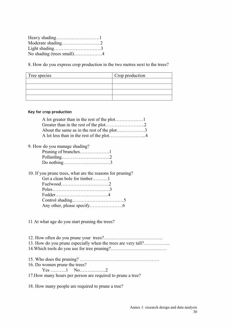
Heavy shading……………………….1 Moderate shading…………………….2 Light shading…………………………3 No shading (trees small)………………4 8. How do you express crop production in the two metres next to the trees? Tree species Crop production
Key for crop production
A lot greater than in the rest of the plot………………1 Greater than in the rest of the plot…………………….2 About the same as in the rest of the plot………………3 A lot less than in the rest of the plot…………………...4
9. How do you manage shading?
Pruning of branches……………….1 Pollarding………………………….2 Do nothing…………………………3
10. If you prune trees, what are the reasons for pruning? Get a clean bole for timber……….1 Fuelwood………………………….2 Poles……………………………….3 Fodder…………………………….4
Control shading……………………………5 Any other, please specify…………………6
11 At what age do you start pruning the trees? 12. How often do you prune your trees?……………………………….. 13. How do you prune especially when the trees are very tall?…………….. 14.Which tools do you use for tree pruning?……………………………… 15. Who does the pruning? …………………………………………… 16. Do women prune the trees?
Yes ……….1 No……………..2 17.How many hours per person are required to prune a tree? 18. How many people are required to prune a tree?
Annex 1: research design and data analysis 30

19. How many members of the household help in pruning? Households members No. Men Women Children 20. Do you at times hire labour for pruning? Yes……..1 No………….. 21. If yes, how much do you pay per tree or per day……………………………………………………………………… 22.What do you use the prunings for? Fuelwood ………….1 Poles ………………..2 Fodder……………….3 Mulch……………….4 Sell………………….5 23. If you sell the prunings, what are the selling prices of the wood products Fuelwood
Poles 24. Where do you sell your tree products?
Buyers come and collect…………….1 Local market…………………………2 Near by sawmills…………………….3
25. After tree pruning and pollarding, do you observe any changes in crop yield adjacent to trees? Yes………1 No……………2 26. If yes, is the change positive or negative? …………………………………………………………. 27 If negative, what do you think is the problem?
Root competition……..1 Branches left still cast shade……………2
Trees produce toxic resins ………………………3 Don’t know……………………………………..4
28. Are you aware of root competition between trees and crops? Yes ………….1 No……………2 29. If yes, how do you manage root competition on your farm?
Dig root trenches ……….1 Leave the area close to the trees roots without crops……..2
Annex 1: research design and data analysis 31

Do nothing (Don’t mind crop loss)………….3 Do nothing (Don’t know how to manage root competition)…4
Annex 1: research design and data analysis 32

A1.10 Survey protocol no. 3 Objective: to determine the influence of the project on pruning practices and gather further information on pruning costs and value of products Follow-up surveys were conducted at Kabale, where there had been an intensive programme of dissemination and training, and at Siaya, where there had been less formal training, but local farmers had worked as casual labourers on the Siaya experimental plot and learned how to prune, and seen the impacts of it. Embu was not resurveyed because there were few formal activities in that area, and the Kibwezi part of the project had not been running for long enough to justify resurveying. Farmers were selected from among groups which had been exposed to training, and groups which had not been exposed. QUESTIONNAIRE ON TREE PRUNING PRACTICES IN KABALE Enumerators name………………………………. Date of interview………………………………… Section 1 General Information
1. District……………………………. 2. Sub County.………………………… 3. Parish………………………….. 4. Village………………………. 5. Farmer’s name…………………… 6. Gender. Male………..1. Female……….2 7. Age………………..
8. Interview conducted with Male head and wife…………….1 Wife (husband not present)……………….2 Female head (husband engaged in off-farm activities)…3 Female head (widow)…………………………4 Male head……………………………………….5 9. What is the main source of income of the household?
From the farm…………….1 Off-farm……………………2 Others (specify)…………..3
Section 2 Adoption of Pruning a. Do you have trees on farm? Yes……………………..1 go to b No……………………..2 b. If yes, which trees, how are they planted, and what is their purpose?
Tree type Planting niche Purpose
Annex 1: research design and data analysis 33

Key for Niche
HC: Home compound B: Boundary CL: Cropland O: Others (Please specify) GL: Grazing land
Purpose
Fuelwood…………………..1 Poles/Timber………………2 Soil Conservation…………3 Boundary…………………..4 Windbreak………………….5 Fodder………………………6 Fruits………………………..7 Shade……………………….8 Amenity……………………..9 Soil fertility………………….10
c. Do you prune trees? Yes…………………..1 go to e. No…………………..2 go to d d. If no, what are your reasons for not pruning? Lack of Knowledge……………..1 See no Importance………………2 Lack of time……………………..3 Lack of labour……………………4 Other (specify)……………………5 e. If yes, which trees do you prune and why?
Tree type pruned Reason for pruning
f. From whom did you acquire the knowledge on pruning? From neighbour………………………1 NGO (specify)………………………..2 Farmer group (specify)……………….3 Other (specify)………………………..4 g. When was your first pruning date? h. How many people have you talked to about pruning? i. Do you have trees in the cropland? Yes………..1 go to j No…2
j. If yes, which trees do you have in the cropland?
Tree type Arrangement
Annex 1: research design and data analysis 34

k. Do you have any trees along the boundary with your neighbour? Yes……………..1 go to l No………………2
l. If yes, have you had any conflicts with your neighbour about the effects of your trees on his land?
Yes…………..1 go to m No……………2
m. If yes, how did you resolve the conflict? Pruning the trees on the neighbours side………..1 Cutting down the trees………………………………2 Did nothing…………………………………………….3 Any other, please specify…………………………….4
Section 3. Socio-economics of pruning 1.How often do you prune your trees?………………………… 2.At what age do you start pruning the trees? 3.How do you prune especially when the trees are tall?………..
4.Give the rank of your reason of pruning
1.Get a clean bole for timber………………. 2.Fuelwood……………………………………. 3.Poles…………………………………………. 4.Fodder………………………………………… 5.Control shading………………………………. 6.Any other (specify)……………………………..
5.Which tools do you use for tree pruning?……………………….
6.Who does the pruning?………………………………………….. 7.Do women prune the trees?
Yes…………….1 No……………………2
8. If you have trees on cropland how much does your tree shade the adjacent crop?
Tree type Shading effect
KEY
Heavy shading………………………1 Moderate shading……………………2 Light shading………………………….3
Annex 1: research design and data analysis 35

No shading (trees small)……………..4
9. How do you express crop production in the two metres next to the trees?
Tree species Crop production
Key for crop production
A lot greater than in the rest of the plot………………………..1 Greater than in the rest of the plot………………………………2 About the same as the rest of the plot…………………………..3 A lot less than in the rest of the plot………………………………4
10. How many hours per person are required to prune a tree? 11. How many people are required to prune a tree? 12. How many members of the household help in pruning?
Households members Number Men Women Children
13. Do you at times hire labour for pruning?
Yes………..1 No……………2
14. If yes how much do you pay per tree, or per day? ……………………………………………………..
15. What do you use the prunings for? Fuelwood………………..1 Poles……………………..2 Fodder……………………3 Mulch……………………..4 Sell………………………..5 go to 16 Stakes…………………….8
16. If you sell the prunings, what are the selling prices of the wood products 1 Fuel wood……………… 2 Poles…………………..
17. Where do you sell your tree products? Buyers come and collect…………………1 Local market……………………………….2 Near by sawmills…………………………,,,3
18. After tree pruning and pollarding; do you observe any changes in crop yield adjacent to trees? Yes……………1 go to 19 No………………….2
19.If yes, is the change positive or negative? ………………………………………………
20. If negative, what do you think is the problem? Root competition……………1 Branches left still cast shade………………2 Trees provide toxic resins…………………..3
Don’t know……………………………………4
Annex 1: research design and data analysis 36

21. Are you aware of root competition between trees and crops? Yes……………….1 No…………………2
22. If yes, how do you manage root competition on your farm? Dig root trenches………………1 Leave the area close to the trees roots without crops…2 Do nothing (Don’t mind crop loss)……………………………3 Do nothing (Don’t know how to manage root competition)…. 4
23. Enumerators’ observations.
Annex 1: research design and data analysis 37

Siaya followup questionnaire Enumerator’s name: Date of interview: Start time……………. End time……………..
a) Name of household head ………………………………………. b) Respondent’s name ……………………………………………. c) Relationship of Respondent to Household Head …………….. d) District…………………………………..Village……………… e) Respondent’s age ……………………………………………… f) Household size ……………..Above 18 …….. Under 18 …….
1. Household type
a) Male headed b) Female headed (husband away) c) Female headed, (widow) d) Male headed (widower) e) Other (specify)
2. Land ownership type: a) Own land b) Tenant c) Squatter d) Other (specify)
3. Does the household own any trees on the farm? Yes……………………. Estimate the no…………….. If yes, type of tree products from the farm……………. No……………………………………………………... 4. Who makes decisions on farm activities? 5. What is the major occupation of the decision maker and where does he/she live? 6. Occupation
a) Farming b) Farming and cottage industries c) Schooling d) On-farm employment e) Off-farm employment f) Other
7. Living a) On-farm b) Off-farm
8. What is the approximate size of your land holding?……………….. 9. What is the main source of income of the household?……………..
a) From the farm b) Off-farm c) Other
SECTION TWO 8. Why do you do pruning to your trees?
Annex 1: research design and data analysis 38

a) To reduce conflict with neighbours b) Fuel wood c) To give poles or timber d) Improve timber quality e) Animal fodder f) To reduce shade g) To reduce competition below ground h) Other
9. Which trees can be pruned? 10. Has anyone talked to you about pruning? If yes, who? 11. Has anyone shown you how to do it? 12. What methods did they show you? Crown? Root? 13. What size of trees do you do the pruning? SECTION THREE Application of pruning 14. Does someone prune your trees? 15. How do they or you do it? If crown pruning 16.
a) When do you prune? (Time of year) …… b) How often do you prune the same tree within a year?
17. a) Which species do you prune? b) Which ones don’t you prune and why?
18. At what age or height do you do the pruning? 19. How do you do the pruning? (How extreme do you go?) 20. Which tools do you use? 21. Who does the pruning?
a) Family male b) Family female c) Hired labour d) Other (specify)
22. What is the cost of pruning per tree if hired labour is used? If root pruning 23. When do you do the pruning? (Time of the year and how often)………… 24. Which species do you prune? 25. Which ones don’t you prune? 26. What size of trees do you prune? (Age and height) How deep does the pruning go? (How far away from the tree, all the way round, or just one side.)
Annex 1: research design and data analysis 39

27. Which tools are used? 28. Who does it?
Family men? Family female? Hired labour?
29. What is the cost of pruning? INFLUENCE OF THE PROJECT 30. Is this the same way you have always done the pruning? Or different? 31. Is this something new, which you have never done before?
Do you think pruning is worthwhile?………………..Why? 32. Are you going to carry on doing it?………………….Why? 33. If you don’t prune, why?………………… 34. Have any of your neighbours taken up pruning? SECTION FOUR Concerns about pruning 35. Does anything worry you about pruning?
a) Safety b) Too heavy work c) Death of trees d) Loss of tree products e) Not worth the effort f) No time g) Lack of trees h) Other
ECONOMIC INFORMATION 36. Which tree products have you purchased in the last two months?
a) Fire wood b) Building and construction materials c) Fodder d) Other
37. What prices do you pay per unit? ……………………………………….. 38. Which wood products have you sold in the last 12 months? 1. Firewood 2. Construction materials 3. Fodder 4. Other
4.1. What prices do you get? (per unit)
4.2. Which tree products from your farm do you sell?
Annex 1: research design and data analysis 40

4.3. What are the other products from the farm that you sell?
4.4. What are the selling prices of maize and beans? Maize………………. Beans………………. 43. What are the local buying prices for different sizes and species of?
i) Poles ii) Bundles of firewood iii) Charcoal
44. What are the buying prices of locally grown?
i) Maize ii) Beans
Enumerator’s comments ………..
Annex 1: research design and data analysis 41

5. References 42

Annex 2: Dissemination and training materials
Final Technical Report to DFID
ZF0094 / R7342

The following items have been produced during the project. Many of these items have previously been provided in hard copy to FRP. Those items which have not been previously provided are enclosed with this report. Academic dissertation
• Wajja-Musukwe, TN 2003 Management of below-ground competition in simultaneous agroforestry systems. University of Dundee. PhD thesis. 237 pp.
• Tefera, AT 2004 Crown and root pruning of four-year old boundary trees at Siaya and Nyabeda in Western Kenya: socioeconomics, utilization of soil water, and maize and wood yields. University of Sokoine. PhD thesis 277pp.
• Sande, BD 2002 Pollarding and root pruning as management options for tree-crop competition and firewood production. MSc thesis. University of Stellenbosch. 114 pp.
Book contribution
• Rao, MR, Schroth, G, Williams S, Namirembe S, Schaller, M and Wilson, J. in press. Chapter 15: Managing Belowground Interactions in Agroecosystems. Eds van Noordwijk, M., Cadisch, G., Ong, CK. CABI.
Briefing notes
• Odee, DW, Mulatya J, Muchiri D, Kiptot E, Kimondo J and Wilson J. 2004. Tree pruning technologies for farms in Kenyan ASALs. 2pp.
• Wajja-Musukwe N, Sande BD and Wilson J. 2004. Tree management on farms in Uganda. 2pp.
Conference and workshop reports
• Wilson J, Deans JD, Wajja-Musukwe N, Raussen T, Ong CK. 1999. Project initiation workshop: pruning effects on root function. Kabale, Uganda 19 pp.
• Bamwerinde WM, Sande BD, Musiime J and Raussen T. 1999. Sharing local knowledge: Farmers from Kabale (Uganda) study tree - pruning systems and agroforestry in Embu (Kenya): Report of a visit by Kabale farmers to Kenya in May 1999
• Mulatya J, Tefera A and Wilson J. 2000. Farmers To Farmers Extension Workshop, organized by Kenya Forestry Research Institute (KEFRI) & International Centre For Research In Agroforestry (ICRAF) at KEFRI Kibwezi Research Station, Farmers’ Fields, & ICRAF Machakos Research Station 26th - 29th March 2000. 11 pp.
• Siriri D. Sande BD, Kukundakwe M, and Wajja-Musukwe N. Report of Final Workshop, Kabale, Uganda, October 2003. 21pp.
• Mulatya D, Muchiri D, Wilson J. 2003. On farm trees and their management – presentation to farmers. Siaya Institute of Technology. Workshop 19th March 2003.
• Leaflet
• Pruning trees growing in the cropland. Tree management for farming. Technical Bulletin no. 3. FORRI.
1

Internal project reports
• Sande BD. 1999. Root and Shoot Pruning Experience at the Vi Agroforestry Project - Masaka. Trip Report.
Journal paper
• Ong CK., Wilson, J., Deans, JD., Mulatya, J., Raussen, T., Wajja-Musukwe, N. 2002. Tree crop interactions: manipulation of water use and root function. Agricultural Water Management 53: 171-186
• Odhiambo, HO., Ong, CK., Wilson, J., Deans, JD., Broadhead, J., and Black, C. 1999. Tree-crop interactions for below ground resources in drylands: root structure and function.
• Several more papers are in preparation – currently 2 concerning tree and crop growth in Kabale, 2 for tree and crop growth at Kifu, 1 on tree growth for Siaya and one on tree and crop growth for Kibwezi.
Articles
• Pruning gets to the root of the problem: J Wilson and JD Deans NERC Winter 2000: 6-7.
• Give them a smaller fork! Contribution to DFID FRP 2002-3 report, Ch 4.
Posters and Wallplanners
• How to reduce competition between trees and crops: poster. KEFRI. • Tree pruning to improve timber value: poster. KEFRI. • How to prune trees for good timber: poster. KEFRI. • Okukonera emiti eri omuntabire n’ebindi bihingwa: (Rukiga) wall
planner. FORRI. Training materials
• Deans JD and Wilson J. Training materials on understanding and managing competition and pruning – used and adapted many times in different workshops in Kenya and Uganda
• Mulatya J. Masomo ma undu miti isindanaa na mimea ya liu miundaani. Training materials for nursery management and tree pruning workshops: Kikamba. KEFRI
Models
• Giacomello A-M. Socioeconomic analysis of agroforestry. Videos
• Food and wood: video 39 minutes • Kilimo Mseto: video (Swahili) 33 minutes • Endeberera y’emiti omumusiri: video (Rukiga) 34 minutes
2