Embed Size (px)
Citation preview
Properties of Superconducting Accelerator Cavities
Zachary Conway
July 10, 2007
2
Overview
My background is in heavy-ion superconducting accelerator structures. AKA low and intermediate-velocity accelerator resonators
Outline– RF Superconductivity– RF Superconductivity in accelerators– Part 2
3
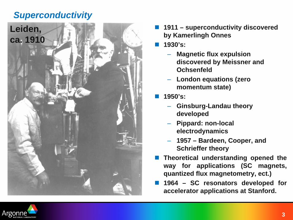
Superconductivity1911 – superconductivity discovered by Kamerlingh Onnes1930’s:
– Magnetic flux expulsion discovered by Meissner and Ochsenfeld
– London equations (zero momentum state)
1950’s:– Ginsburg-Landau theory
developed– Pippard: non-local
electrodynamics– 1957 – Bardeen, Cooper, and
Schrieffer theoryTheoretical understanding opened the way for applications (SC magnets, quantized flux magnetometry, ect.)1964 – SC resonators developed for accelerator applications at Stanford.
Leiden, ca. 1910
4
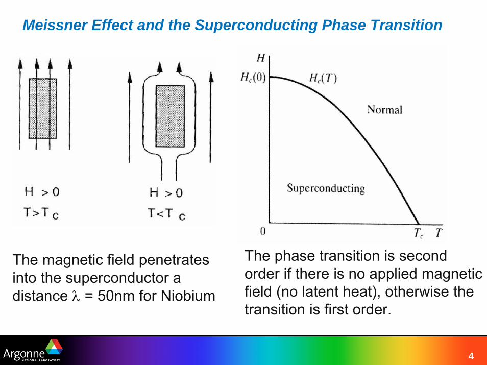
Meissner Effect and the Superconducting Phase Transition
The magnetic field penetrates into the superconductor a distance λ = 50nm for Niobium
The phase transition is second order if there is no applied magnetic field (no latent heat), otherwise the transition is first order.
5
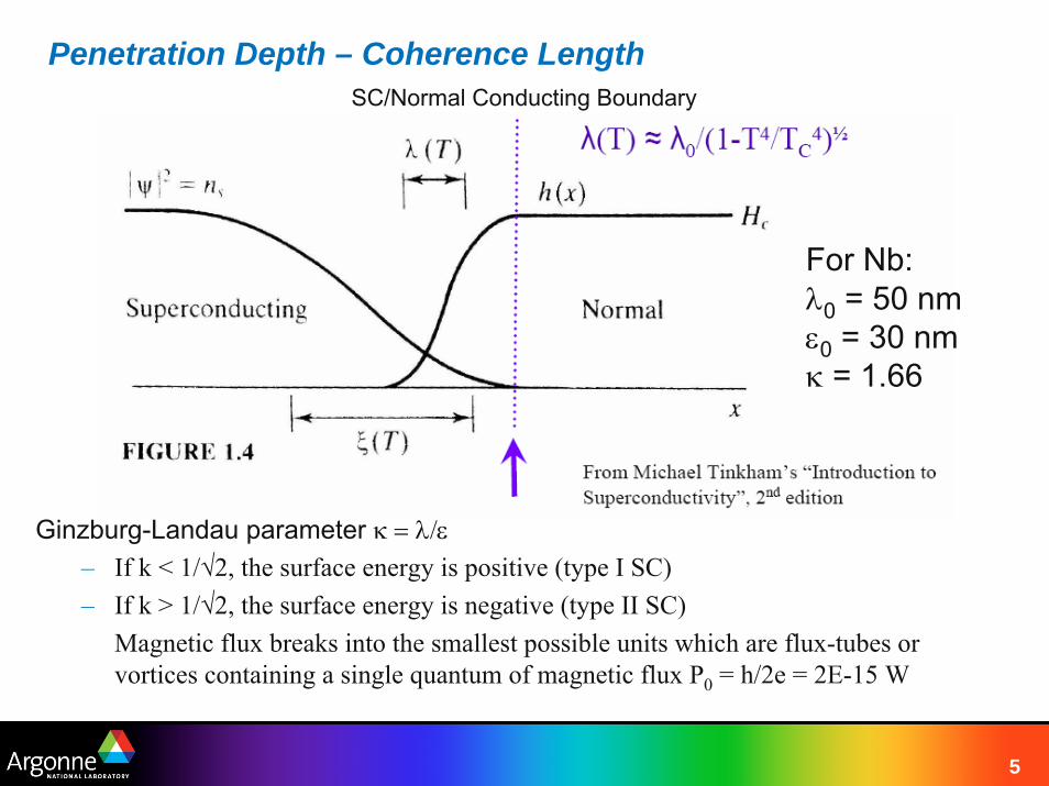
Penetration Depth – Coherence Length
Ginzburg-Landau parameter κ = λ/ε– If k < 1/√2, the surface energy is positive (type I SC)– If k > 1/√2, the surface energy is negative (type II SC)
Magnetic flux breaks into the smallest possible units which are flux-tubes or vortices containing a single quantum of magnetic flux P0 = h/2e = 2E-15 W
SC/Normal Conducting Boundary
For Nb:λ0 = 50 nmε0 = 30 nmκ = 1.66
6
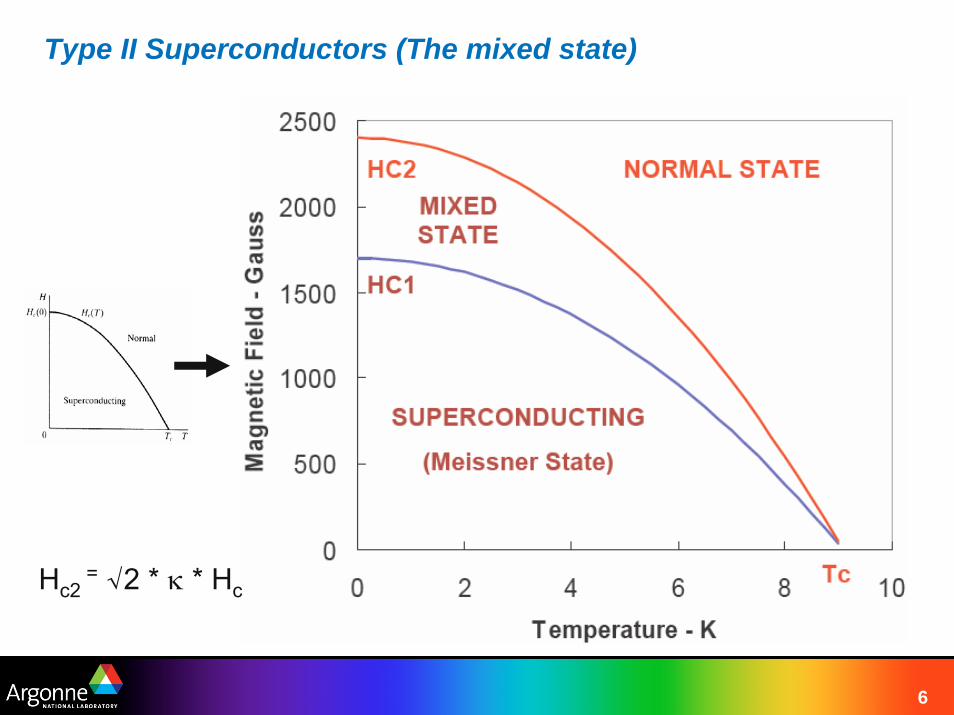
Type II Superconductors (The mixed state)
Hc2= √2 * κ * Hc
7
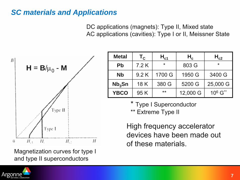
SC materials and Applications
Magnetization curves for type I and type II superconductors
H = B/μ0 - MMetal TC Hc1 Hc Hc2
Pb 7.2 K * 803 G *
Nb 9.2 K 1700 G 1950 G 3400 G
Nb3Sn 18 K 380 G 5200 G 25,000 GYBCO 95 K ** 12,000 G 106 G**
* Type I Superconductor** Extreme Type II
DC applications (magnets): Type II, Mixed state AC applications (cavities): Type I or II, Meissner State
High frequency accelerator devices have been made out of these materials.
8
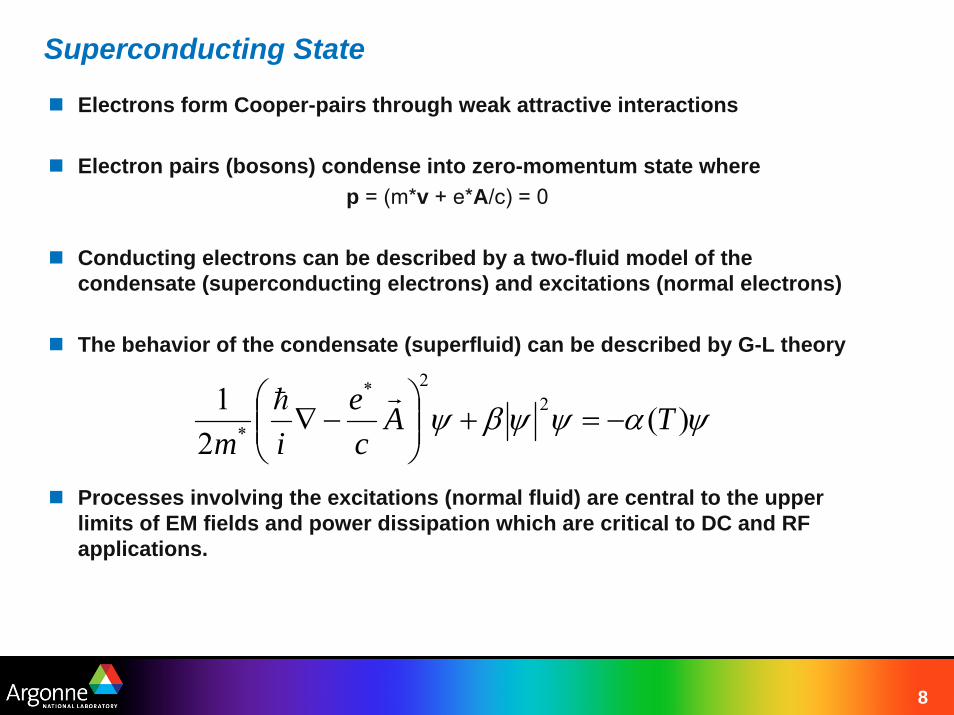
Superconducting State
Electrons form Cooper-pairs through weak attractive interactions
Electron pairs (bosons) condense into zero-momentum state wherep = (m*v + e*A/c) = 0
Conducting electrons can be described by a two-fluid model of the condensate (superconducting electrons) and excitations (normal electrons)
The behavior of the condensate (superfluid) can be described by G-L theory
Processes involving the excitations (normal fluid) are central to the upper limits of EM fields and power dissipation which are critical to DC and RF applications.
ψαψψβψ )(2
1 22*
* TAce
im−=+⎟⎟
⎠
⎞⎜⎜⎝
⎛−∇
rh
9
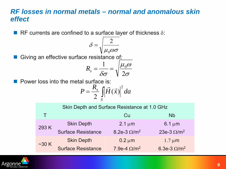
RF losses in normal metals – normal and anomalous skin effect
RF currents are confined to a surface layer of thickness δ:
Giving an effective surface resistance of:
Power loss into the metal surface is:
ωσμδ
0
2=
σωμ
δσ 21 0==sR
∫=S
s daxHP )(2
rR 2r
Skin Depth and Surface Resistance at 1.0 GHzT Cu Nb
Skin Depth 2.1 μm 6.1 μmSurface Resistance 8.2e-3 Ω/m2 23e-3 Ω/m2
Skin Depth 0.2 μm 1.7 μmSurface Resistance 7.9e-4 Ω/m2 6.3e-3 Ω/m2
~30 K
293 K
10
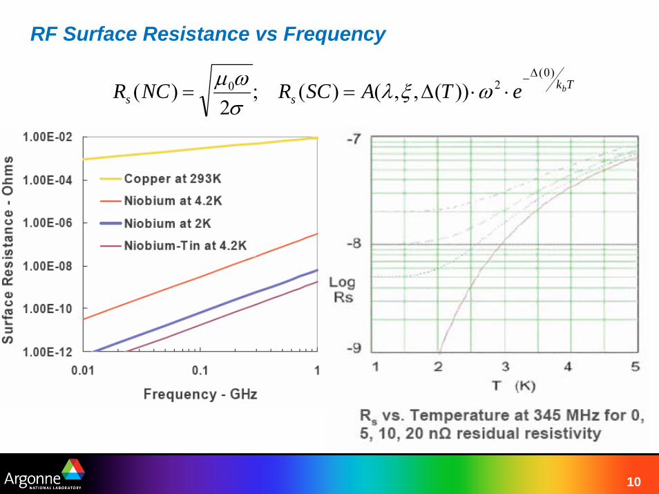
RF Surface Resistance vs Frequency
Tkss
beTASCRNCR)0(
20 ))(,,()(;2
)(Δ−
⋅⋅Δ== ωξλσωμ
11
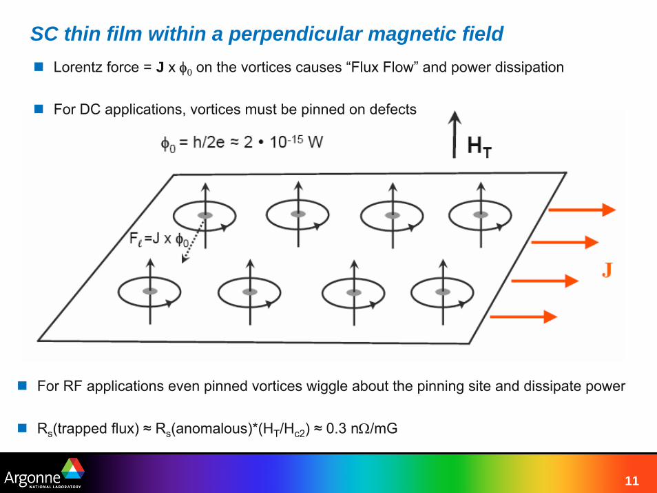
SC thin film within a perpendicular magnetic fieldLorentz force = J x φ0 on the vortices causes “Flux Flow” and power dissipation
For DC applications, vortices must be pinned on defects
For RF applications even pinned vortices wiggle about the pinning site and dissipate power
Rs(trapped flux) ≈ Rs(anomalous)*(HT/Hc2) ≈ 0.3 nΩ/mG
12
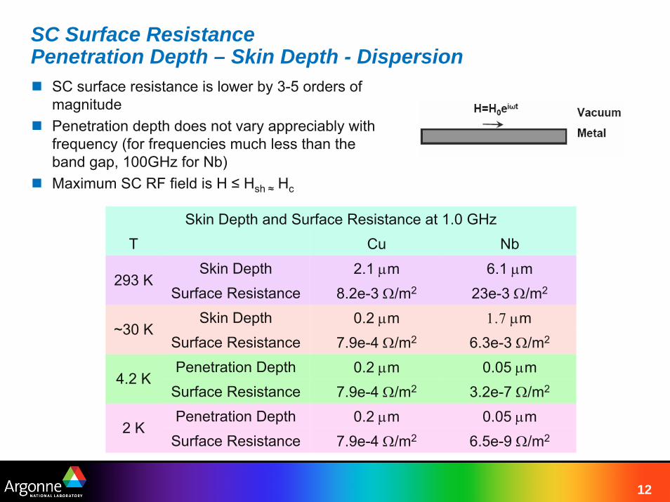
SC Surface ResistancePenetration Depth – Skin Depth - Dispersion
SC surface resistance is lower by 3-5 orders of magnitudePenetration depth does not vary appreciably with frequency (for frequencies much less than the band gap, 100GHz for Nb)Maximum SC RF field is H ≤ Hsh ≈ Hc
Skin Depth and Surface Resistance at 1.0 GHzT Cu Nb
Skin Depth 2.1 μm 6.1 μmSurface Resistance 8.2e-3 Ω/m2 23e-3 Ω/m2
Skin Depth 0.2 μm 1.7 μmSurface Resistance 7.9e-4 Ω/m2 6.3e-3 Ω/m2
Penetration Depth 0.2 μm 0.05 μmSurface Resistance 7.9e-4 Ω/m2 3.2e-7 Ω/m2
Penetration Depth 0.2 μm 0.05 μmSurface Resistance 7.9e-4 Ω/m2 6.5e-9 Ω/m2
2 K
4.2 K
~30 K
293 K
13
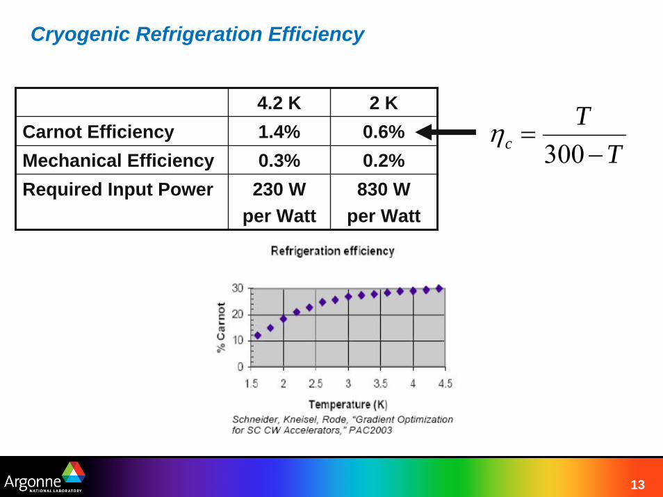
Cryogenic Refrigeration Efficiency
4.2 K 2 KCarnot Efficiency 1.4% 0.6%Mechanical Efficiency 0.3% 0.2%Required Input Power 230 W
per Watt830 W
per Watt
TT
c −=
300η
14
Summary So Far
Depending on the frequency and temperature we can reduce RF losses by a factor of 104 to 106 by going from room temperature cooper to niobium at 2-4 K.Given the efficiency of present cryogenic refrigerators, the net wall-plug power savings can be in the range of 30 – 1000
Playing the SC game might be worth while...– Field limits and breakdown– Detuning: microphonics and Lorentz detuning
For the next 16 slides we will discuss basis features of cavities, SC cavities, and the nomenclature of SCRF
We will wrap today up with an intensive review of R&D work dealing with matching the cavity RF field phase with the charged particle beam bunch
15
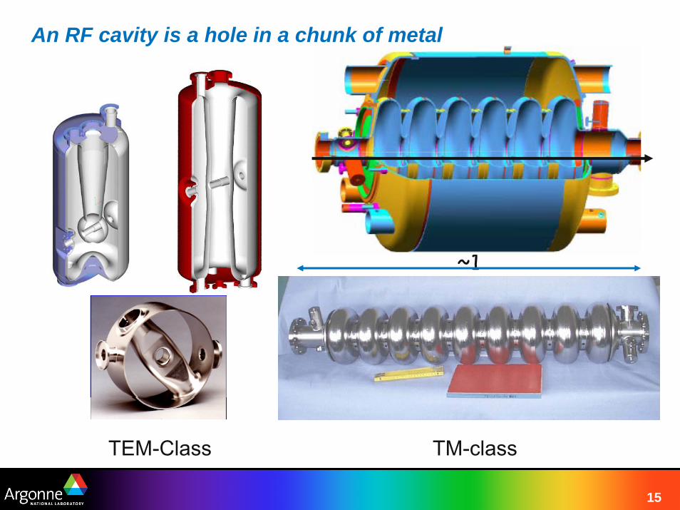
An RF cavity is a hole in a chunk of metal
~1m
TEM-Class TM-class
16
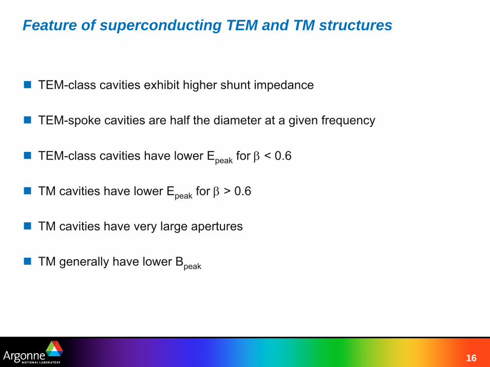
Feature of superconducting TEM and TM structures
TEM-class cavities exhibit higher shunt impedance
TEM-spoke cavities are half the diameter at a given frequency
TEM-class cavities have lower Epeak for β < 0.6
TM cavities have lower Epeak for β > 0.6
TM cavities have very large apertures
TM generally have lower Bpeak
17
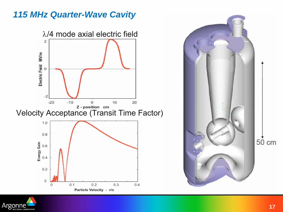
115 MHz Quarter-Wave Cavity
Velocity Acceptance (Transit Time Factor)
λ/4 mode axial electric field
18
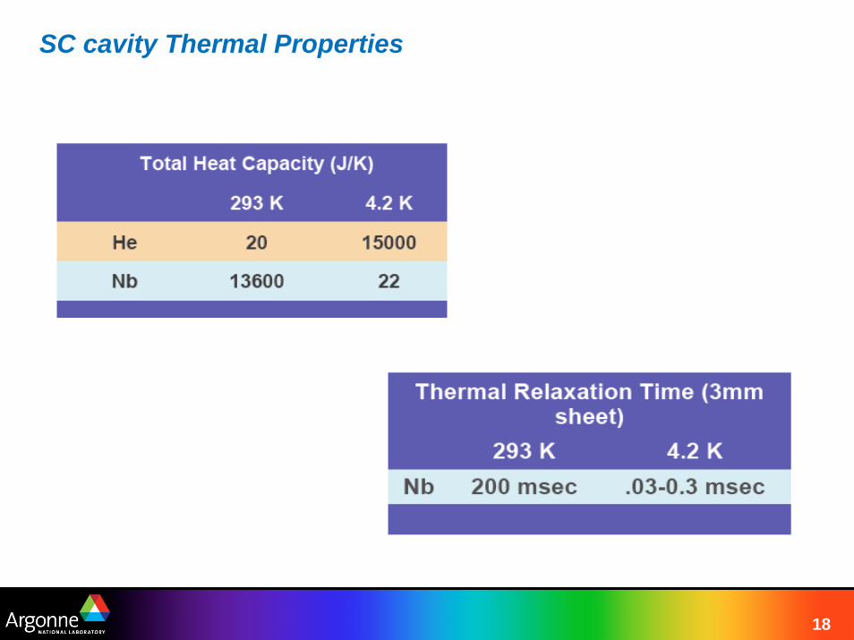
SC cavity Thermal Properties
19
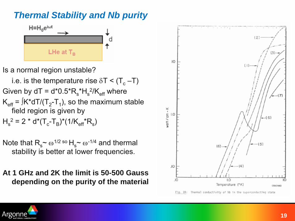
Thermal Stability and Nb purity
Is a normal region unstable?i.e. is the temperature rise δT < (Tc –T)
Given by dT = d*0.5*Rs*Hs2/Keff where
Keff = ∫K*dT/(T2-T1), so the maximum stable field region is given by
Hs2 = 2 * d*(Tc-TB)*(1/Keff*Rs)
Note that Rs~ ω1/2 so Hs~ ω-1/4 and thermal stability is better at lower frequencies.
At 1 GHz and 2K the limit is 50-500 Gauss depending on the purity of the material
20
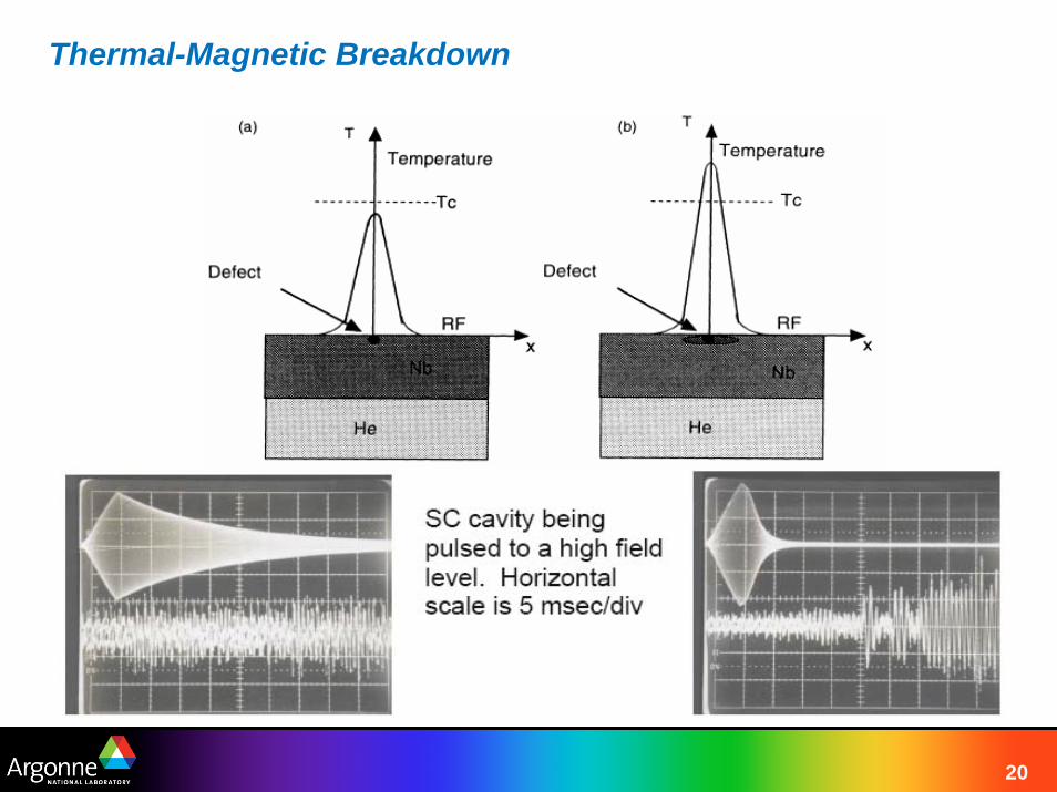
Thermal-Magnetic Breakdown
21
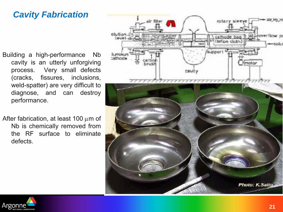
Cavity Fabrication
Building a high-performance Nb cavity is an utterly unforgiving process. Very small defects (cracks, fissures, inclusions, weld-spatter) are very difficult to diagnose, and can destroy performance.
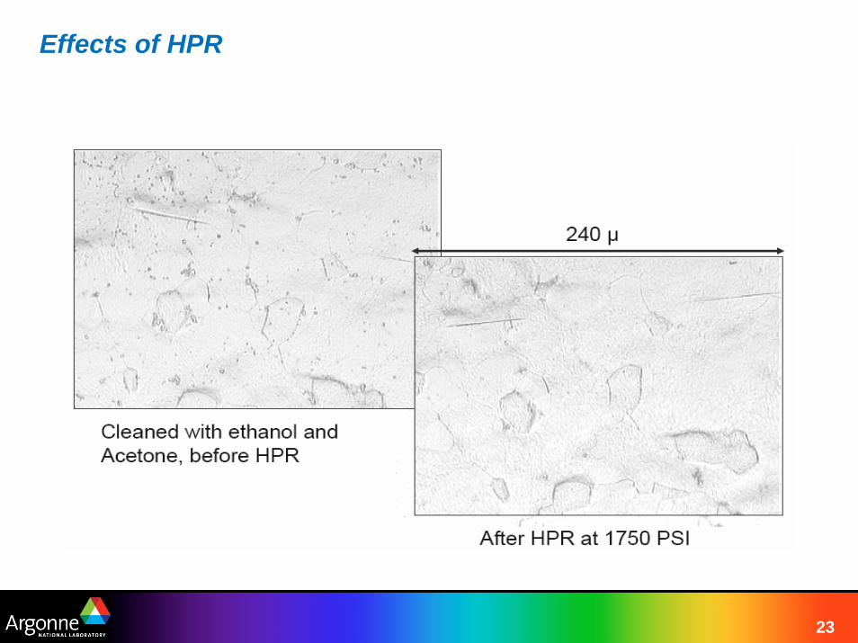
After fabrication, at least 100 μm of Nb is chemically removed from the RF surface to eliminate defects.

22
High-Pressure water rinsing
23
Effects of HPR
24
Cavity parameters all refer to a single eigenmode – the one used to accelerate particles
ω = resonant frequency of the cavity
l0 = effective length of the cavity ( = n*β*λ/2 or (n-1)*β*λ/2)
Eacc = the accelerating gradient: the energy gain per unit charge for a synchronous particle divided by the effective length of the cavity
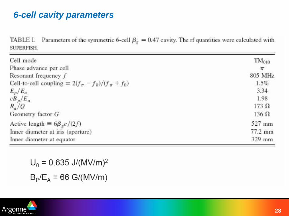
U0 = the electromagnetic energy content of the cavity at Eacc= 1.0 MV/m: in general U(Eacc) = U0 * Eacc
2
Q = δω/ω = ωτ where δω = the -3dB cavity bandwidth and τ = the decay time for the rf energy in the cavity (Power = Stored Energy / τ)

25
Cavity parameters continued
Q = δω/ω = ωτ where δω = the -3dB cavity bandwidth and τ = the decay time for the rf energy in the cavity (Power = Stored Energy / τ)
G = Q * Rs = geometric factor for the cavity: relates the cavity Q to the RF surface resistance of the cavity
Zshunt (sometimes labled as R or Rs) = V2/P and is usually given in the form Zshunt/Q or R/Q, notice that R/Q = l02/ω*U0
Notice that the RF power dissipated in the cavity walls is given by:
⎟⎠⎞
⎜⎝⎛ ⎟
⎠⎞⎜
⎝⎛⋅
⋅=
QRR
ElGPS
acc2
0 )(
26
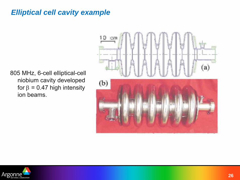
Elliptical cell cavity example
805 MHz, 6-cell elliptical-cell niobium cavity developed for β = 0.47 high intensity ion beams.
27
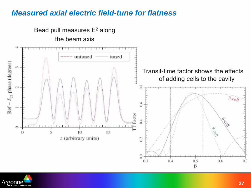
Measured axial electric field-tune for flatness
Bead pull measures E2 alongthe beam axis
Transit-time factor shows the effects of adding cells to the cavity
28
6-cell cavity parameters
29
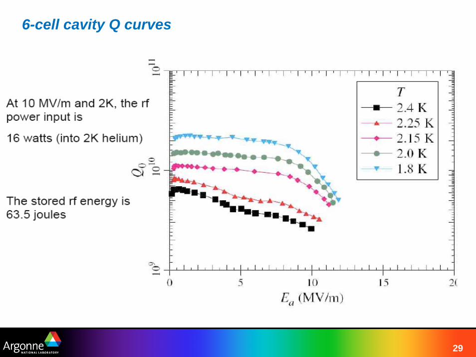
6-cell cavity Q curves
30
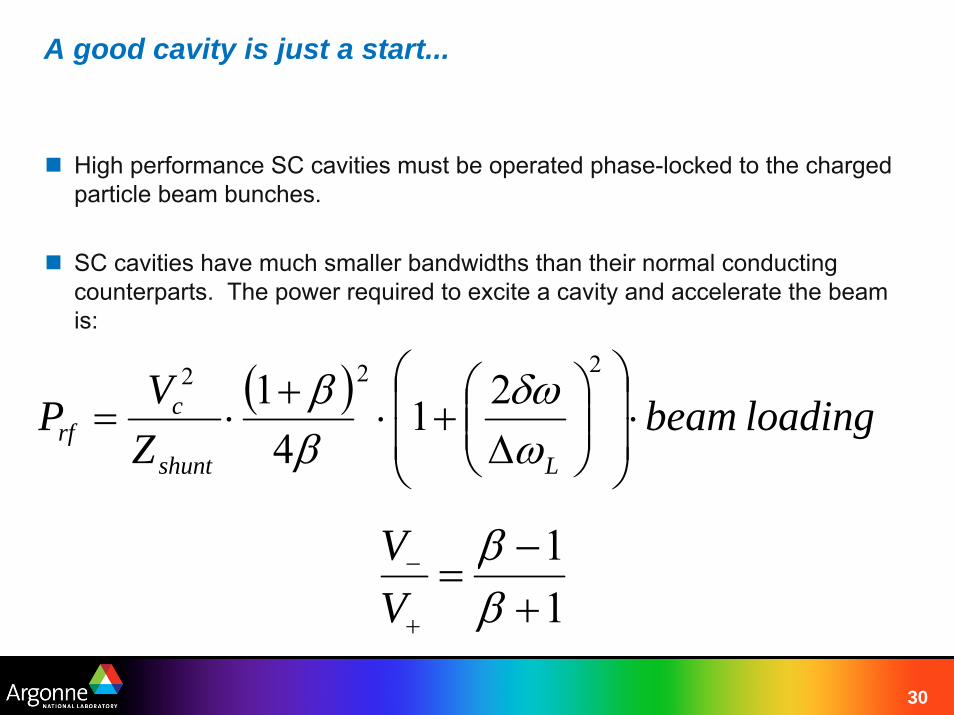
A good cavity is just a start...
High performance SC cavities must be operated phase-locked to the charged particle beam bunches.
SC cavities have much smaller bandwidths than their normal conducting counterparts. The power required to excite a cavity and accelerate the beam is:
( ) loadingbeamZVP
Lshunt
crf ⋅
⎟⎟
⎠
⎞
⎜⎜
⎝
⎛⎟⎟⎠
⎞⎜⎜⎝
⎛Δ
+⋅+
⋅=222 21
41
ωδω
ββ
11
+−
=+
−
ββ
VV
31
Break
20 minutes
32
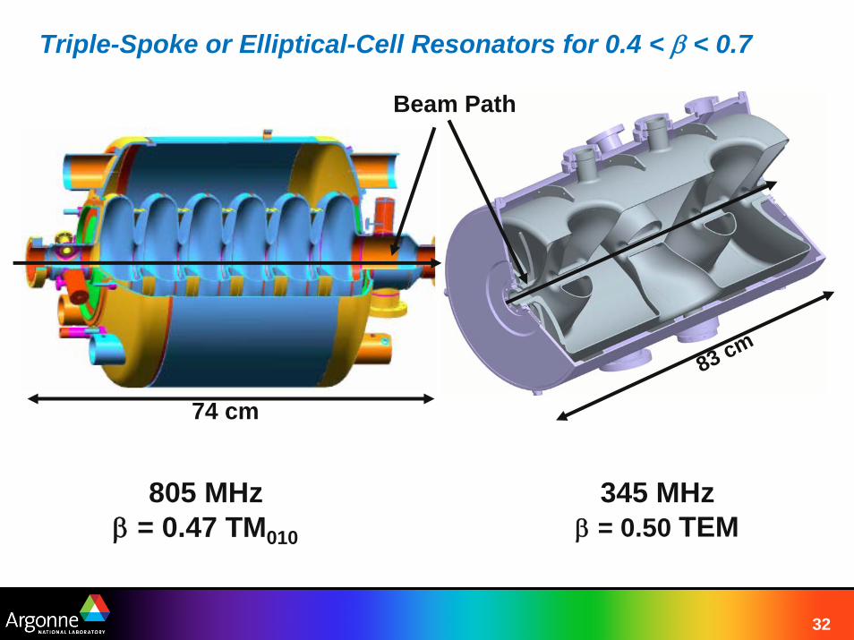
Triple-Spoke or Elliptical-Cell Resonators for 0.4 < β < 0.7
805 MHzβ = 0.47 TM010
345 MHzβ = 0.50 TEM
83 cm
Beam Path
74 cm

33
Triple-Spoke or Elliptical-Cell Resonators for 0.4 < β < 0.7
The transverse size of TM structures is of the order of 0.9 λwhile for TEM structures it is on the order of 0.5 λ, λ = c/f.
At a fixed transverse size TEM structures operate at approximately half the frequency, this has several important consequences:– Lower BCS surface resistance– A TEM structure will have half the number of cells of a
TM cavity of the same length and therefore will have a broader velocity acceptance.
– Improved beam dynamics
Improved mechanical stability
34
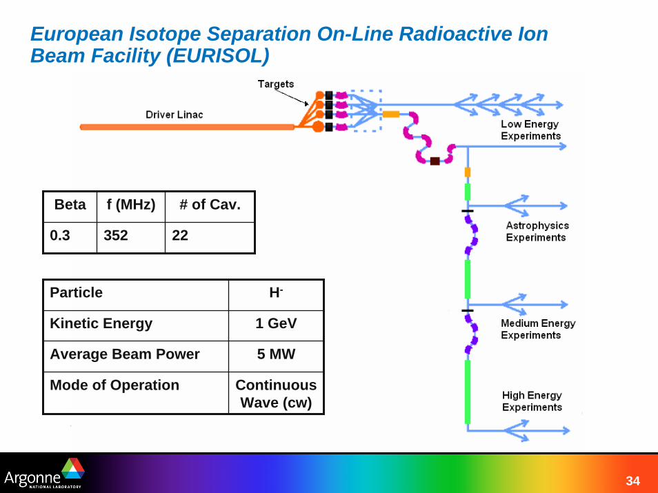
European Isotope Separation On-Line Radioactive Ion Beam Facility (EURISOL)
Particle H-
Kinetic Energy 1 GeV
Average Beam Power 5 MW
Mode of Operation Continuous Wave (cw)
Beta f (MHz) # of Cav.
0.3 352 22
35
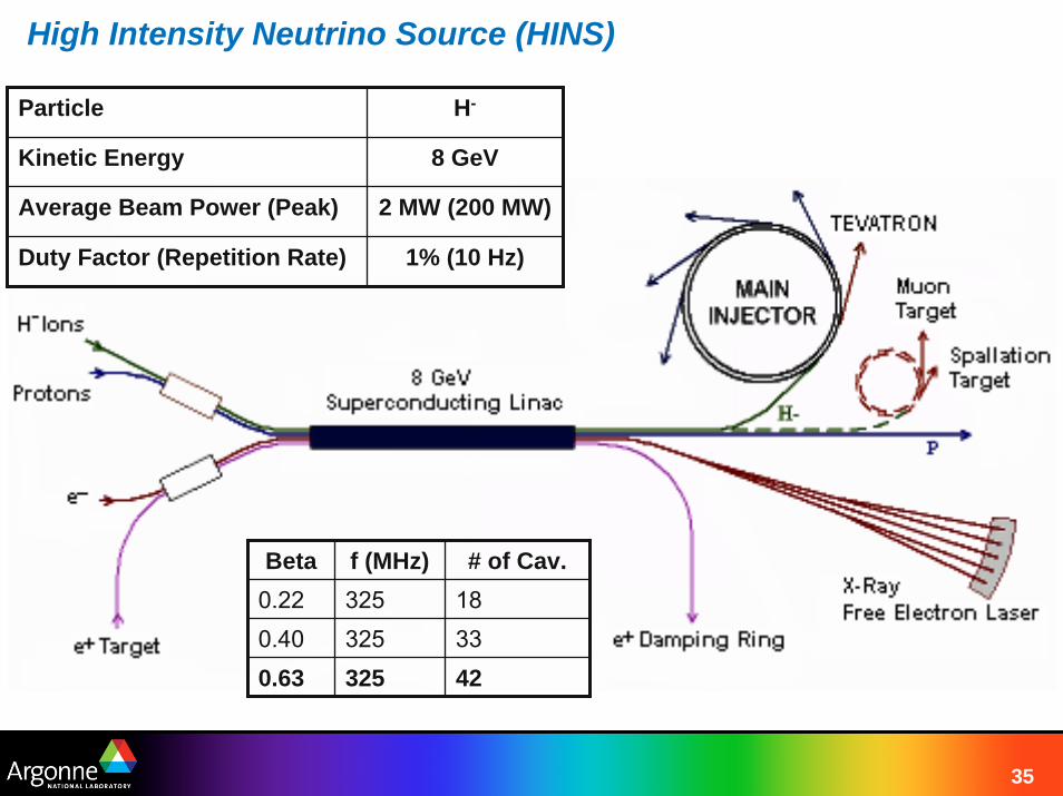
High Intensity Neutrino Source (HINS)
Particle H-
Kinetic Energy 8 GeV
Average Beam Power (Peak) 2 MW (200 MW)
Duty Factor (Repetition Rate) 1% (10 Hz)
Beta f (MHz) # of Cav.0.22 325 180.40 325 330.63 325 42
36
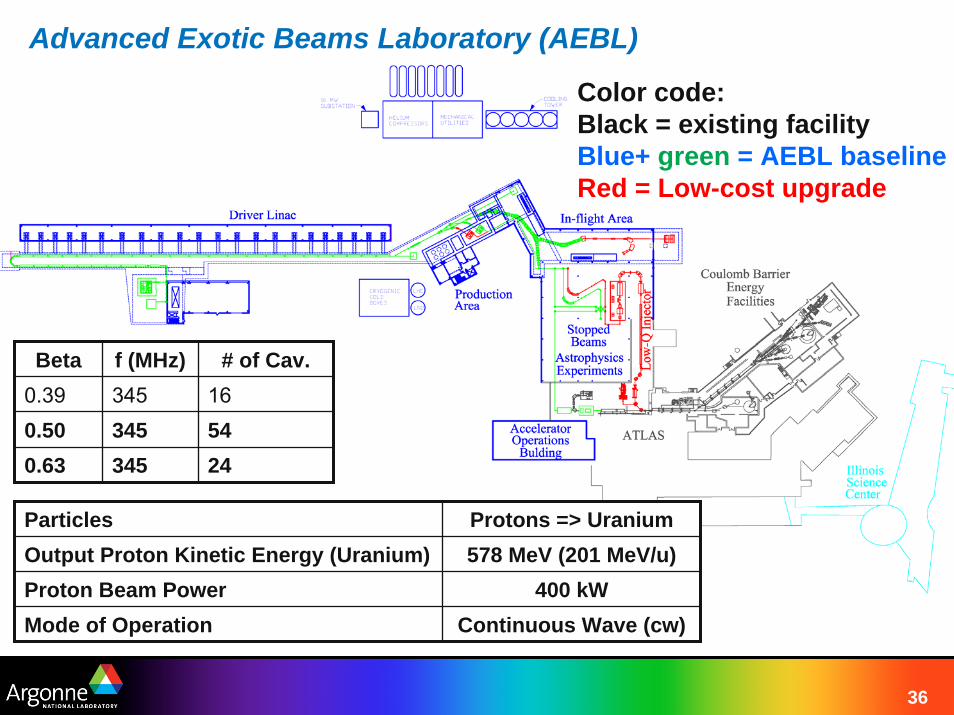
Advanced Exotic Beams Laboratory (AEBL)
Beta f (MHz) # of Cav.0.39 345 160.50 345 540.63 345 24
Color code:Black = existing facilityBlue+ green = AEBL baselineRed = Low-cost upgrade
Particles Protons => UraniumOutput Proton Kinetic Energy (Uranium) 578 MeV (201 MeV/u)Proton Beam Power 400 kWMode of Operation Continuous Wave (cw)

37
ANL Triple-Spoke Cavities
β= 0.50Triple-Spoke Cavity
345 MHz
β= 0.63Triple-Spoke Cavity
345 MHz
102 cm83 cm
38
Cavity RF Performance
The RF power required to operate a cavity RF field phase-locked to the beam bunches is a function of:– The power delivered to the beam
– The power required to control the cavity RF field phase and amplitude errors.
– The power required to energize the cavity
Dramatic improvements in the power required to energize and operate spoke-loaded cavities operating at a fixed beam current have been realized from 6 years of spoke-loaded cavity development
39
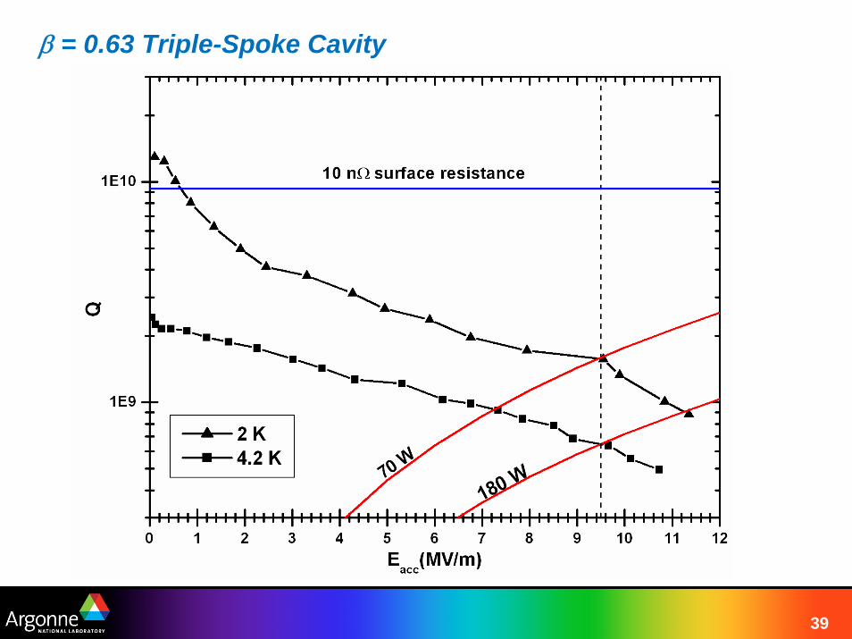
β = 0.63 Triple-Spoke Cavity

40
β = 0.63 Triple-Spoke Cavity
41
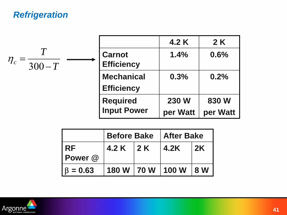
Refrigeration
4.2 K 2 KCarnot Efficiency
1.4% 0.6%
MechanicalEfficiency
0.3% 0.2%
Required Input Power
230 Wper Watt
830 Wper Watt
Before Bake After BakeRF Power @
4.2 K 2 K 4.2K 2K
β = 0.63 180 W 70 W 100 W 8 W
TT
c −=
300η
42
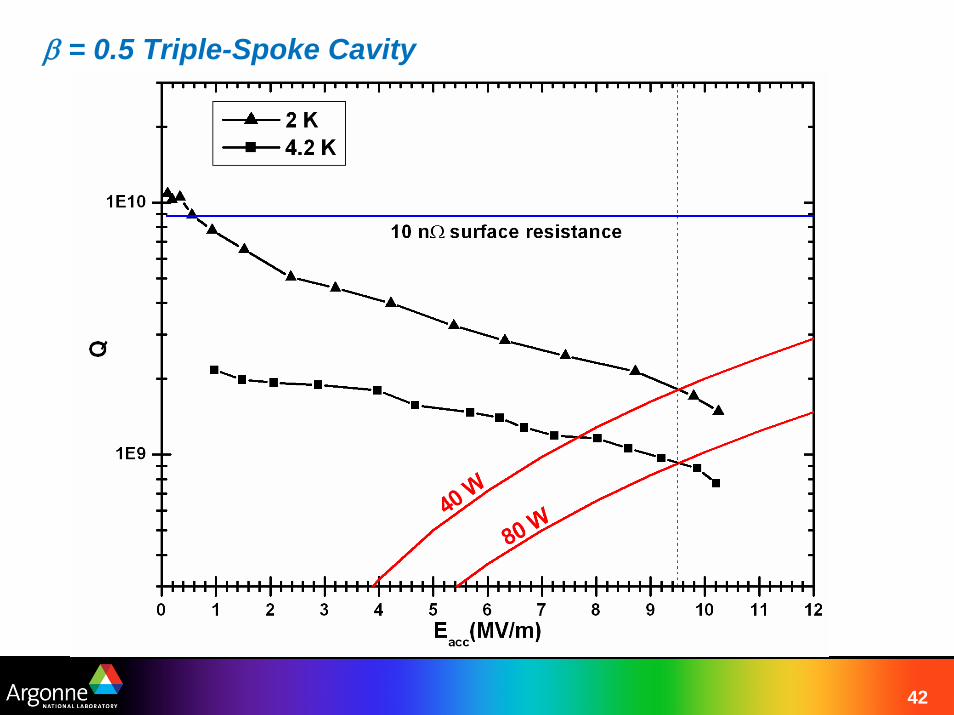
β = 0.5 Triple-Spoke Cavity
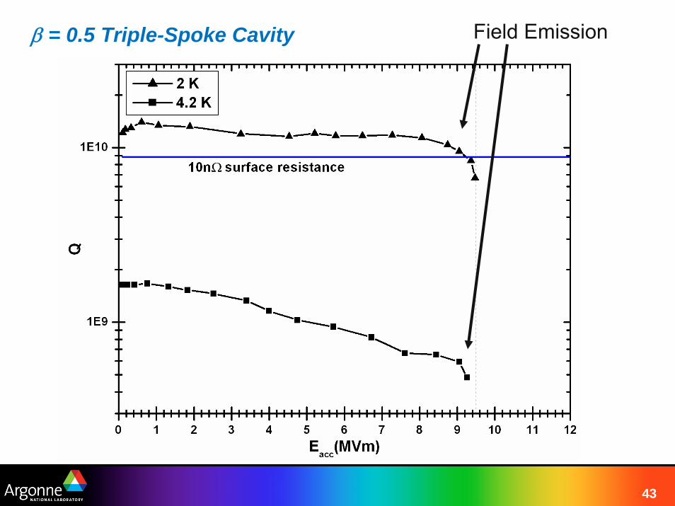
43
β = 0.5 Triple-Spoke Cavity Field Emission
44
Cavity RF Power Requirements
The power required to energize and cool a cavity is only one part of the power required to operate a cavity.
Cavity RF frequency variations generate phase errors between the cavity RF field and the particle beam bunches.
More RF power is required to control the cavity RF field amplitude and phase when the RF frequency variations are a large fraction of the beam loaded cavity bandwidth.
Cavity RF frequency variations are do to external forces coupling to the cavity RF field.
45
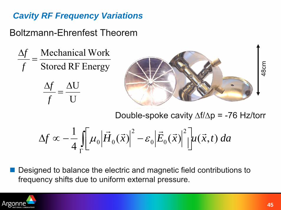
Cavity RF Frequency Variations
Designed to balance the electric and magnetic field contributions to frequency shifts due to uniform external pressure.
datxuxExHf ),()()(41 2
00
2
00rrrrr
∫Γ
⎥⎦⎤
⎢⎣⎡ −−∝Δ εμ
Energy RF Stored WorkMechanical
=Δff
Boltzmann-Ehrenfest Theorem
UUΔ
=Δff
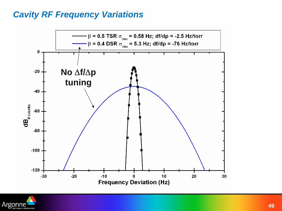
Double-spoke cavity Δf/Δp = -76 Hz/torr
48cm
46
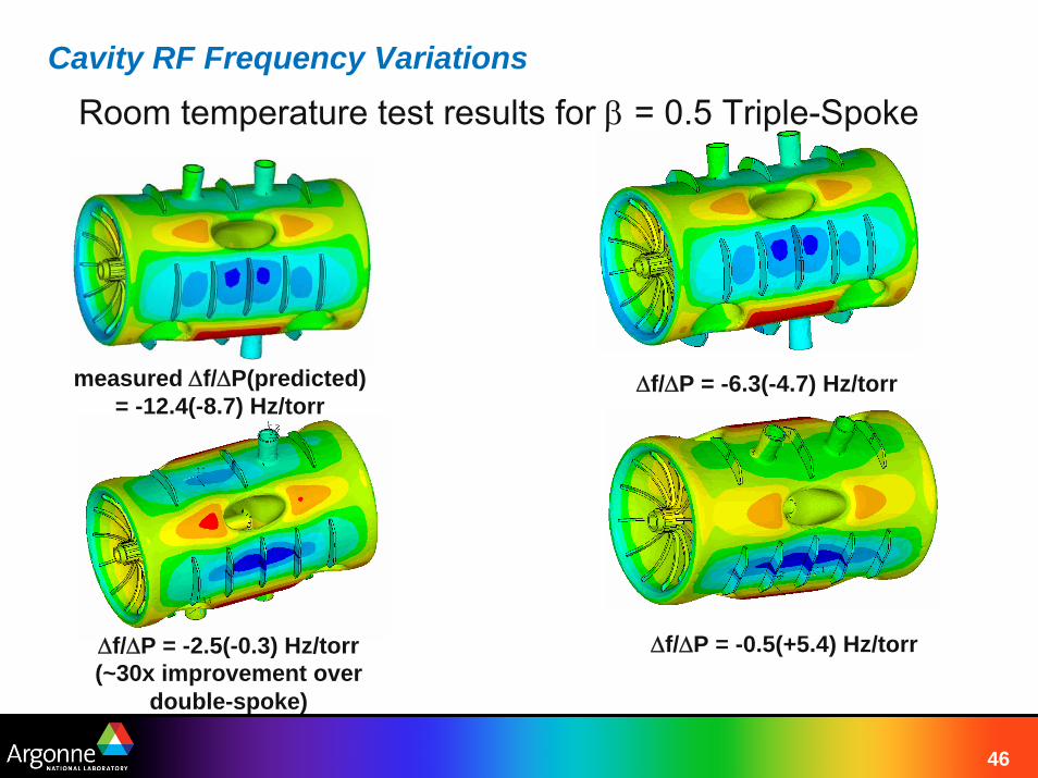
Cavity RF Frequency Variations
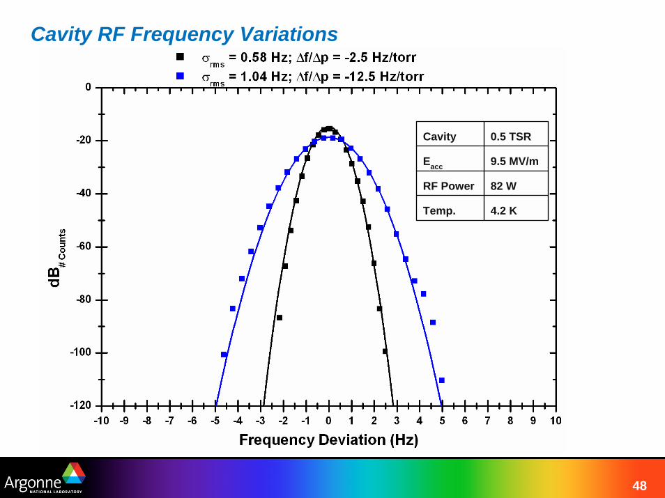
measured Δf/ΔP(predicted) = -12.4(-8.7) Hz/torr
Δf/ΔP = -2.5(-0.3) Hz/torr (~30x improvement over
double-spoke)
Room temperature test results for β = 0.5 Triple-Spoke
Δf/ΔP = -6.3(-4.7) Hz/torr
Δf/ΔP = -0.5(+5.4) Hz/torr
47
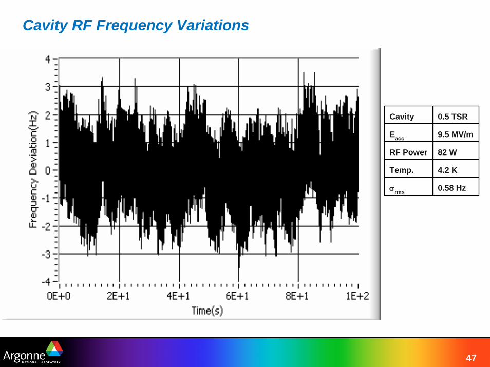
Cavity RF Frequency Variations
Cavity 0.5 TSR
Eacc 9.5 MV/m
RF Power 82 W
Temp. 4.2 K
σrms 0.58 Hz
48
Cavity RF Frequency Variations
Cavity 0.5 TSR
Eacc 9.5 MV/m
RF Power 82 W
Temp. 4.2 K
49
Cavity RF Frequency Variations
No Δf/Δptuning
50
Cavity RF Frequency Variations
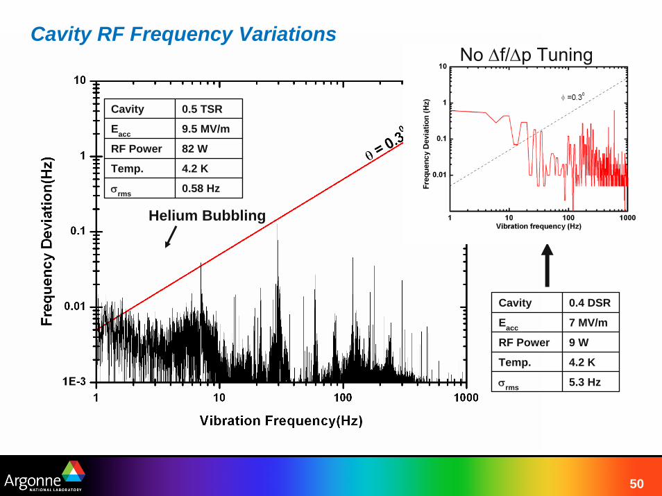
Cavity 0.5 TSR
Eacc 9.5 MV/m
RF Power 82 W
Temp. 4.2 K
σrms 0.58 Hz
Helium Bubbling
5.3 Hzσrms
4.2 KTemp.
9 WRF Power
7 MV/mEacc
0.4 DSRCavity
No Δf/Δp Tuning

51
Cavity RF Frequency Variations
Over-couple to the cavity with the power coupler– RF Power = N x δωrms x U
Fast Reactive Tuners– Damp the cavity bandwidth requiring additional RF power
Fast Mechanical Tuners– No additional RF power requirements
ANL 20 kW Triple-Spoke Fundamental Power Coupler
23.8”
52
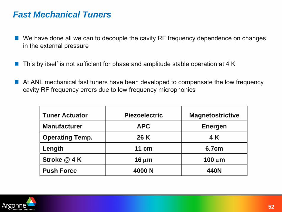
Fast Mechanical Tuners
We have done all we can to decouple the cavity RF frequency dependence on changes in the external pressure
This by itself is not sufficient for phase and amplitude stable operation at 4 K
At ANL mechanical fast tuners have been developed to compensate the low frequency cavity RF frequency errors due to low frequency microphonics
Tuner Actuator Piezoelectric Magnetostrictive
Manufacturer APC Energen
Operating Temp. 26 K 4 K
Length 11 cm 6.7cm
Stroke @ 4 K 16 μm 100 μmPush Force 4000 N 440N
53
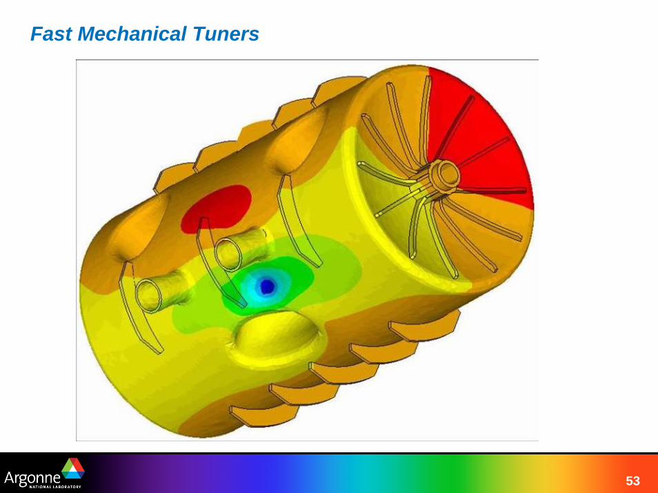
Fast Mechanical Tuners

54
Magnetostrictive Actuated Fast Tuner
Magnetostrictive actuator designed and built by Energen, Inc.
Response time ~6ms.
Magnetostrictive rod coaxial with an external solenoid operating at 4K.
Not designed for high frequency operation.
4.6”
9”
55
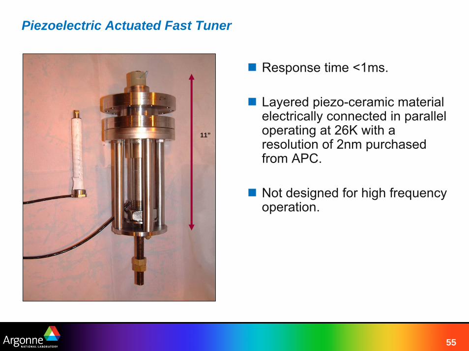
Piezoelectric Actuated Fast Tuner
Response time <1ms.
Layered piezo-ceramic material electrically connected in parallel operating at 26K with a resolution of 2nm purchased from APC.
Not designed for high frequency operation.
11”
56
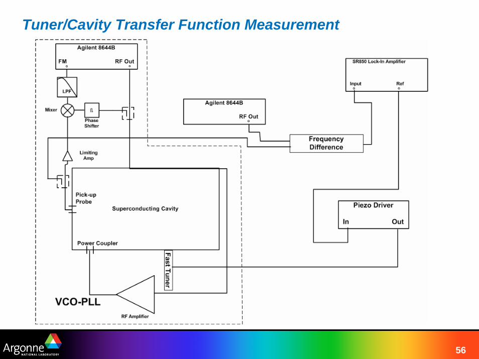
Tuner/Cavity Transfer Function Measurement
57
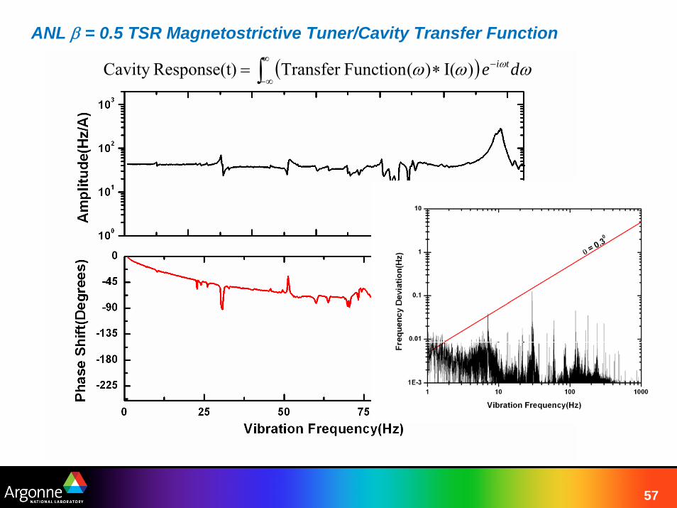
ANL β = 0.5 TSR Magnetostrictive Tuner/Cavity Transfer Function
( ) ωωω ω de ti−∞
∞−∫ ∗= )I()(FunctionTransfer )Response(tCavity
58
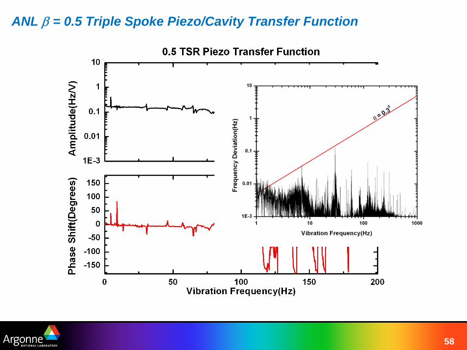
ANL β = 0.5 Triple Spoke Piezo/Cavity Transfer Function
59
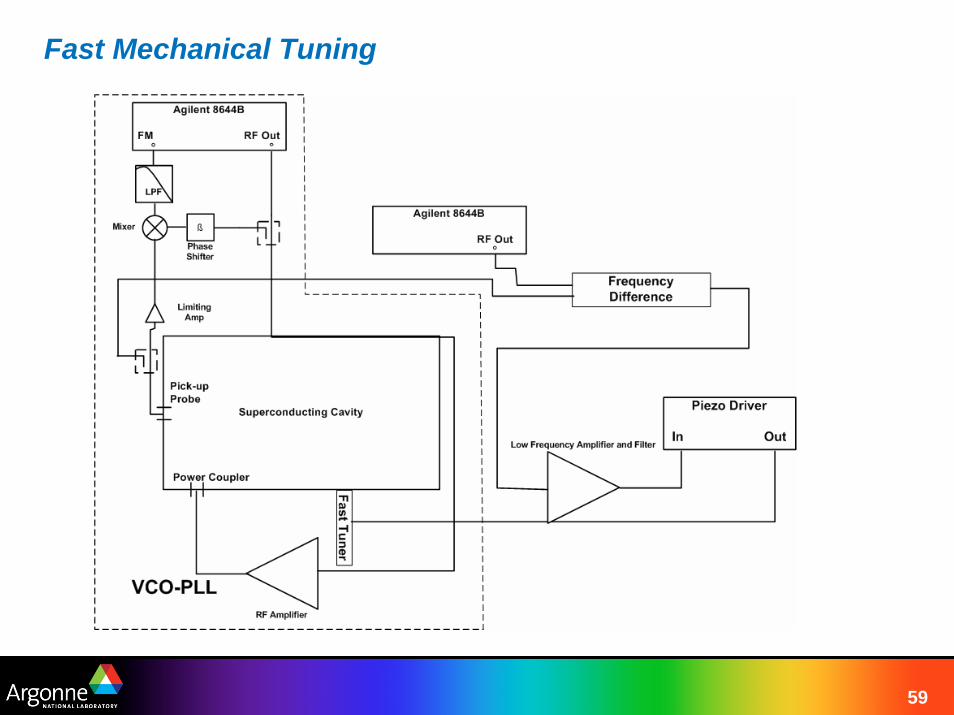
Fast Mechanical Tuning
60
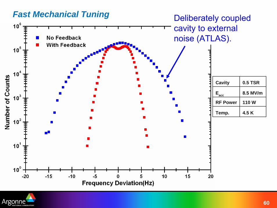
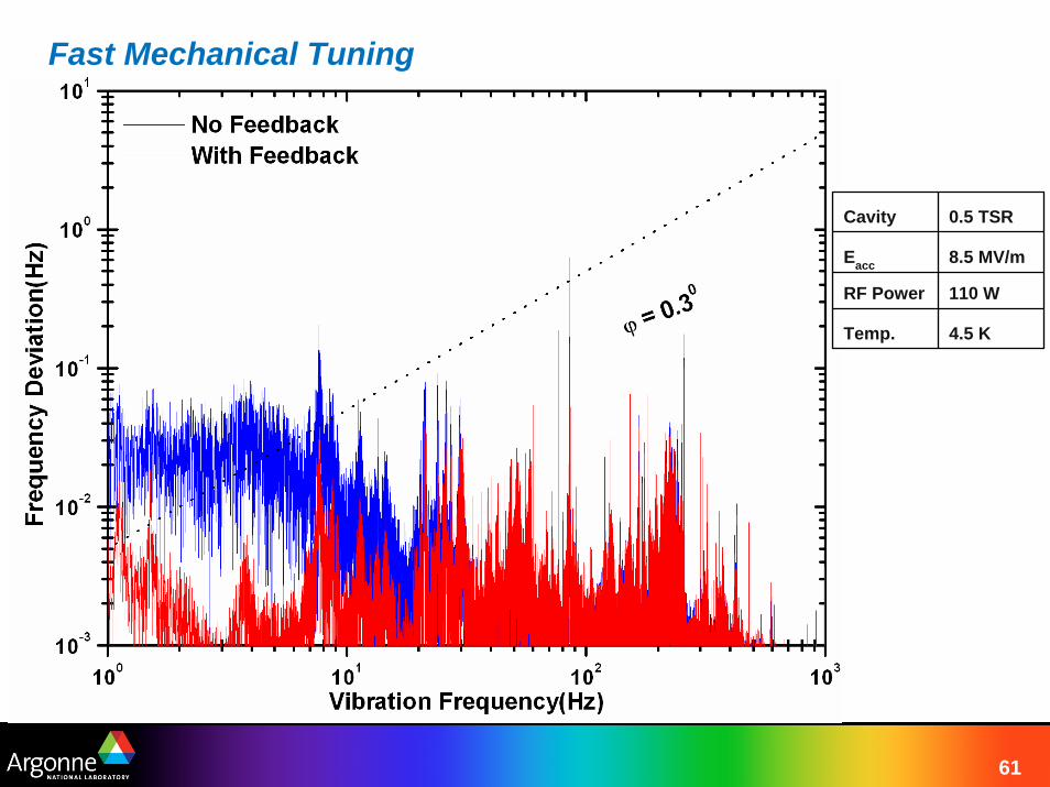
Fast Mechanical Tuning
Cavity 0.5 TSR
Eacc 8.5 MV/m
RF Power 110 W
Temp. 4.5 K
Deliberately coupled cavity to external noise (ATLAS).
61
Fast Mechanical Tuning
Cavity 0.5 TSR
Eacc 8.5 MV/m
RF Power 110 W
Temp. 4.5 K
62
Lorentz Detuning
Systems to control RF field phase errors in cw operation due to low frequency noise have been developed.
Pulsed accelerators have an additional force detuning the cavities, the dynamic Lorentz force
The Lorentz force is due to the cavity RF surface fields interacting with the RF surface currents
The Lorentz force can cause cavity ringing at much higher frequencies than the cw helium bath bubbling

63
SCRF Cavity Frequency Variations
FNAL βgeo = 0.63 triple-spoke cavity loaded-bandwidth ~ 800 Hz
– Ipk(Iave) = 40 (25) mA– Eacc = 10.5 MV/m– Stored Energy ~ 600 mJ
• Largest stored energy of all the spoke-loaded cavities– Effective Length ~ 0.8 m
Externally Driven Frequency Variations?– Microphonics?– Lorentz Force Detuning?
Tests performed at ANL on a βgeo = 0.5 triple spoke cavity yield:– Microphonics ~ 0.58 Hzrms
– Lorentz Force Detuning ~ 1 kHz @ 10.5 MV/m
64
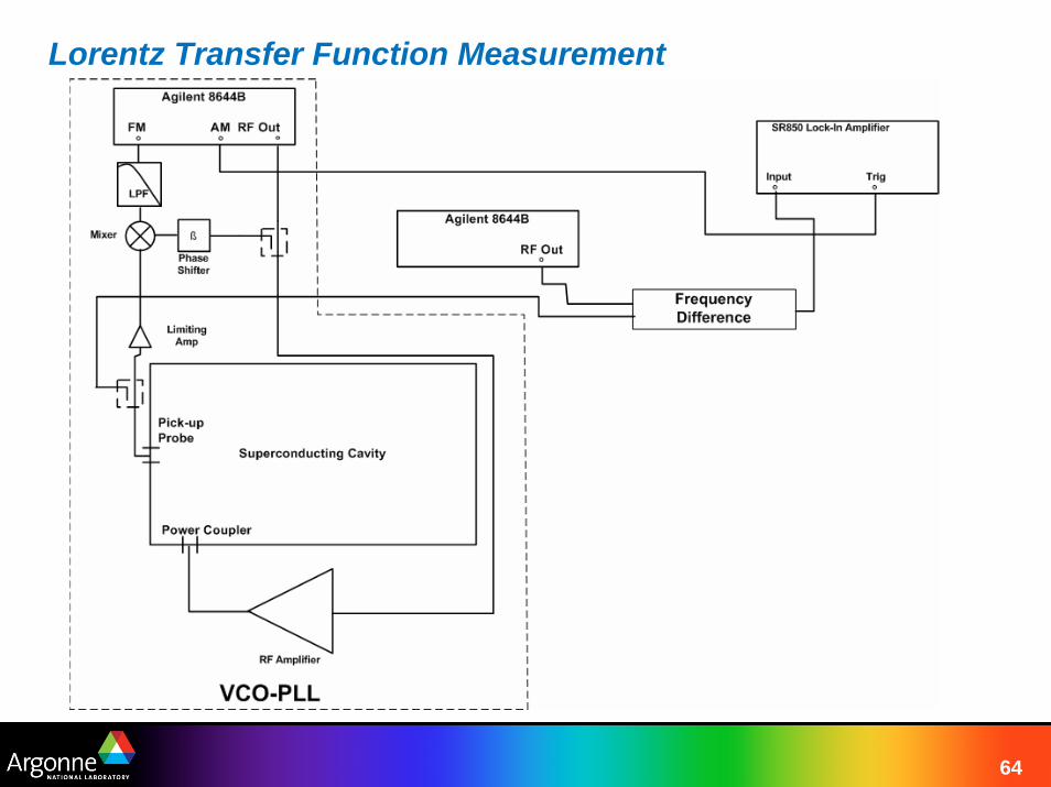
Lorentz Transfer Function Measurement
65
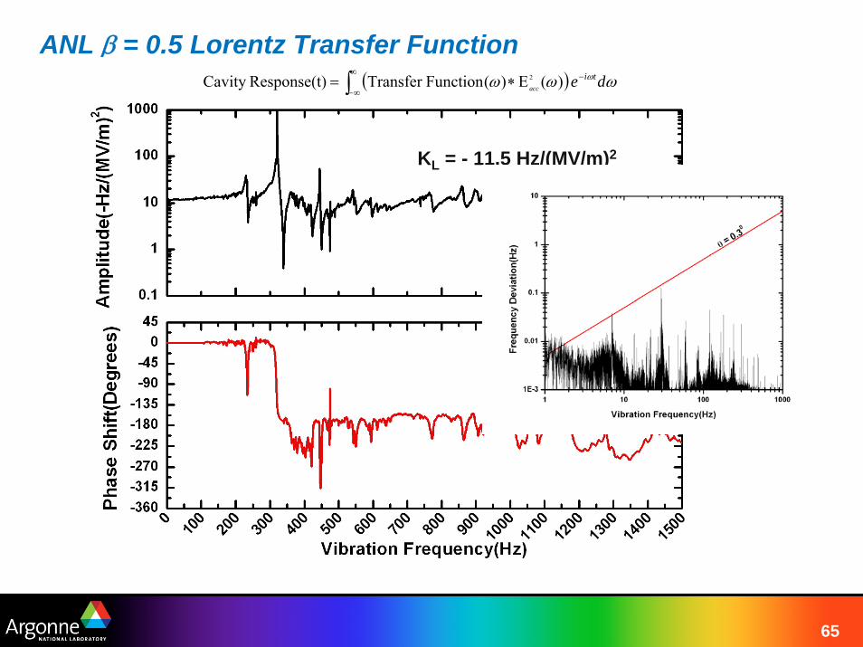
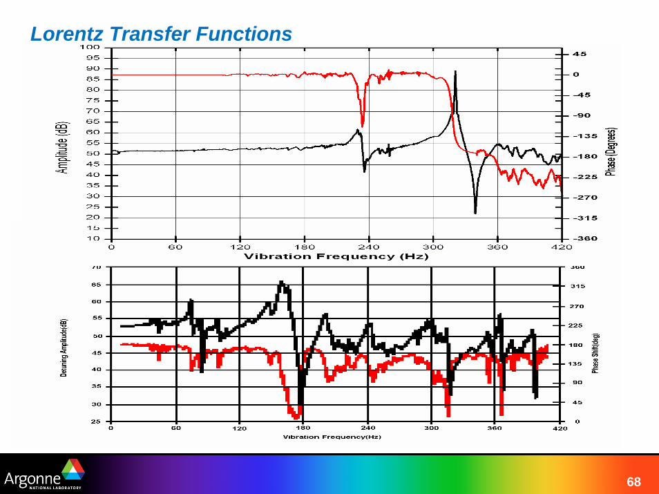
ANL β = 0.5 Lorentz Transfer Function
KL = - 11.5 Hz/(MV/m)2
( ) ωωω ω de tiacc
−∞
∞−∫ ∗= )(E)(FunctionTransfer )Response(tCavity 2

66
ANL β = 0.5 TSR Pulsed Operation( ) ωωω ω de ti
acc
−∞
∞−∫ ∗= )(E)(FunctionTransfer )Response(tCavity 2

67
ANL β = 0.5 TSR Pulsed Operation
68
Lorentz Transfer Functions
69
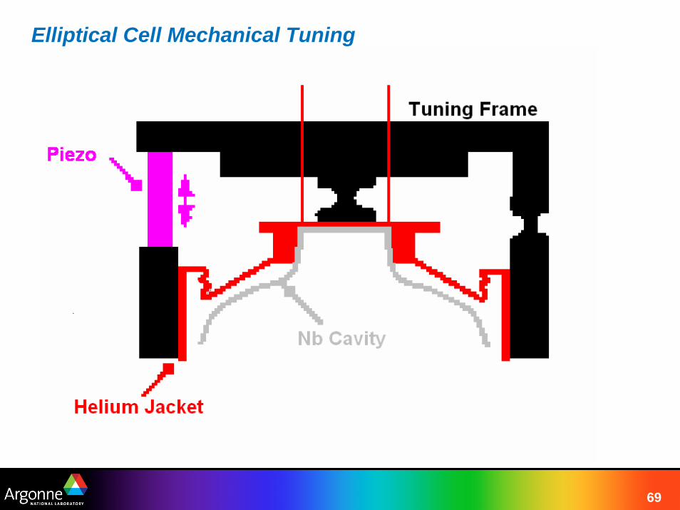
Elliptical Cell Mechanical Tuning
70
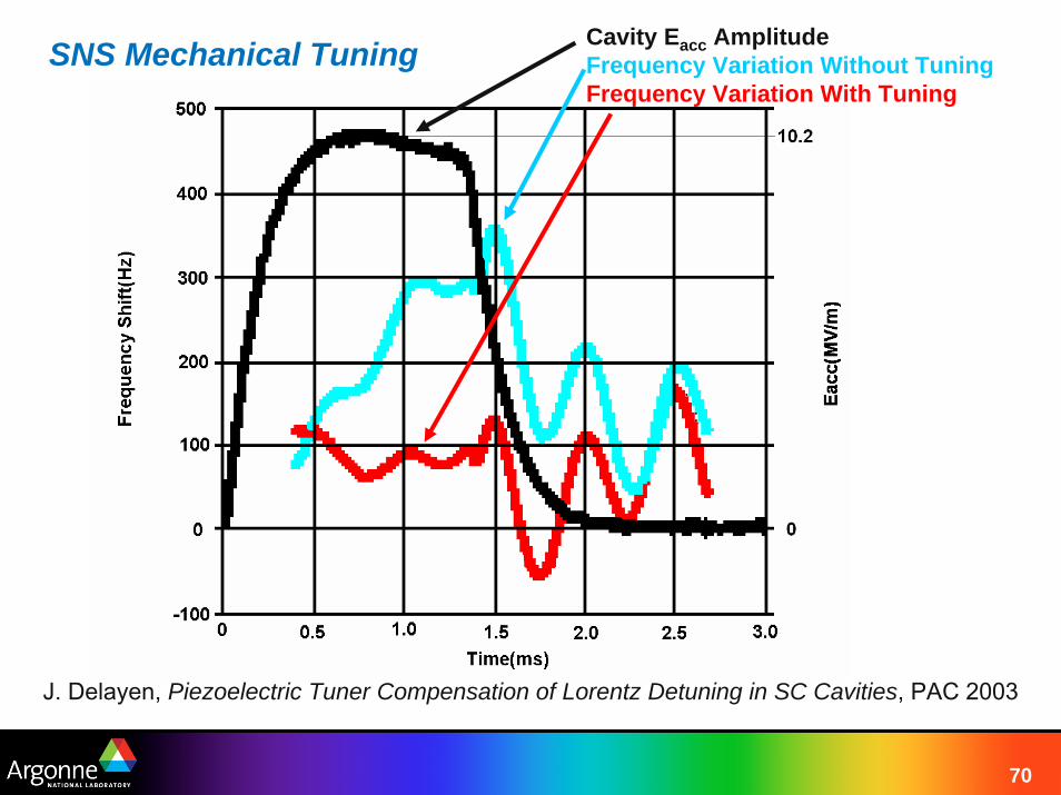
SNS Mechanical Tuning
J. Delayen, Piezoelectric Tuner Compensation of Lorentz Detuning in SC Cavities, PAC 2003
Cavity Eacc AmplitudeFrequency Variation Without TuningFrequency Variation With Tuning
71
FNAL Proton Driver Pulsed Operation
RF power required to phase and amplitude stabilize the ANL β = 0.5 TSR when pulsed to 10.5 MV/m would be much greater than 200kWpeak
Design changes may help– Cavity frequency variations due to the Lorentz force may decrease by
a factor of 2 or 3– This will not improve by a factor of 10
A mechanical fast tuner is necessary
72
Conclusions
Superconducting triple-spoke-loaded cavity technology RF performance exhibits surface resistances < 10 nΩ at 2K after hydrogen degassing.
Tuners still need to be developed to compensate the dynamic RF frequency variations due to pulsed operation of superconducting triple-spoke-loaded cavities
Other mechanical fast tuner solutions were developed for specific SCRF applications– Pulsed operation: DESY X-FEL and SNS– Spoke cavity cw operation: AEBL
This constitutes the only work (I know of) to date on pulsed spoke cavity operation
73
BLANK
BLANK
74
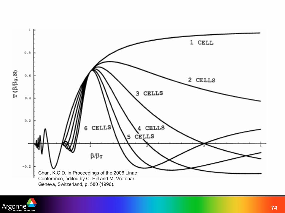
Chan, K.C.D. in Proceedings of the 2006 Linac Conference, edited by C. Hill and M. Vretenar, Geneva, Switzerland, p. 580 (1996).
75
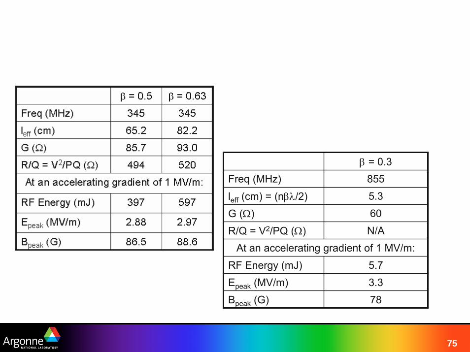
β = 0.3Freq (MHz) 855leff (cm) = (nβλ/2) 5.3G (Ω) 60R/Q = V2/PQ (Ω) N/A
At an accelerating gradient of 1 MV/m:RF Energy (mJ) 5.7Epeak (MV/m) 3.3Bpeak (G) 78
76
Intermediate-Velocity Accelerator Cavities (0.2 < β < 0.7)
Before 1990– Copper Accelerator Structures
• Long structures with a narrow velocity acceptance• Require lots of power to operate cw• Peak fields limited by power dissipation in cavity (100kW/m2)
– Drift tube linacs• Long structures optimized for a single ion species• Not flexible
– Coupled cavity linacs• Long structure optimized for a single ion species• Not flexible
After 1990– Structure were needed
77
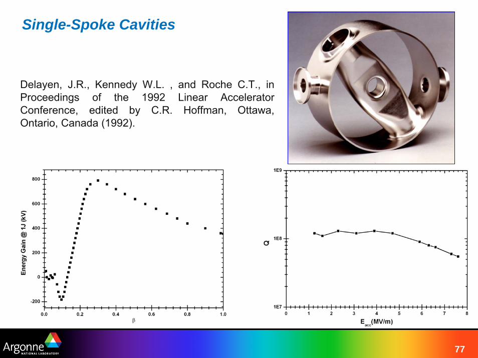
Single-Spoke Cavities
Delayen, J.R., Kennedy W.L. , and Roche C.T., in Proceedings of the 1992 Linear Accelerator Conference, edited by C.R. Hoffman, Ottawa, Ontario, Canada (1992).
78
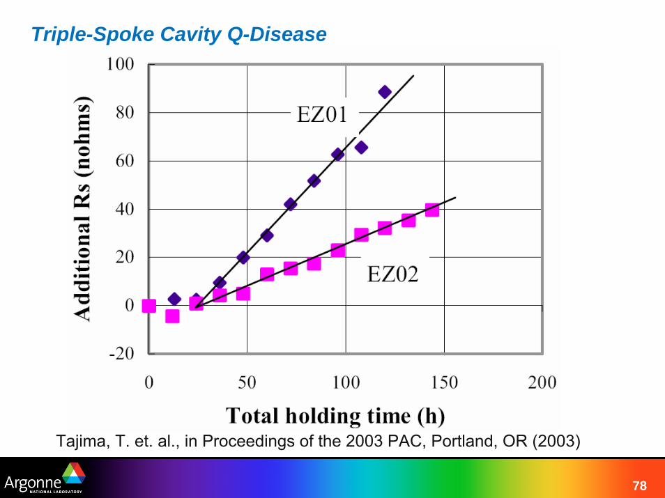
Triple-Spoke Cavity Q-Disease
Tajima, T. et. al., in Proceedings of the 2003 PAC, Portland, OR (2003)
79
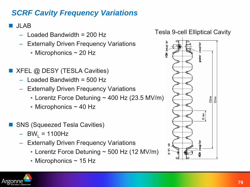
SCRF Cavity Frequency VariationsJLAB– Loaded Bandwidth = 200 Hz– Externally Driven Frequency Variations
• Microphonics ~ 20 Hz
XFEL @ DESY (TESLA Cavities)– Loaded Bandwidth = 500 Hz– Externally Driven Frequency Variations
• Lorentz Force Detuning ~ 400 Hz (23.5 MV/m)• Microphonics ~ 40 Hz
SNS (Squeezed Tesla Cavities)– BWL = 1100Hz– Externally Driven Frequency Variations
• Lorentz Force Detuning ~ 500 Hz (12 MV/m)• Microphonics ~ 15 Hz
Tesla 9-cell Elliptical Cavity
80
AEBL
Original RIA design called for the production of triple-spoke cavities with residual surface resistances on the order of 30 nΩ.
After 6 years of spoke-loaded cavity development triple-spoke cavities can now be produced with residual surface resistances < 10 nΩ.
( ) resBCSs RTfRR +Δ= ,,
81
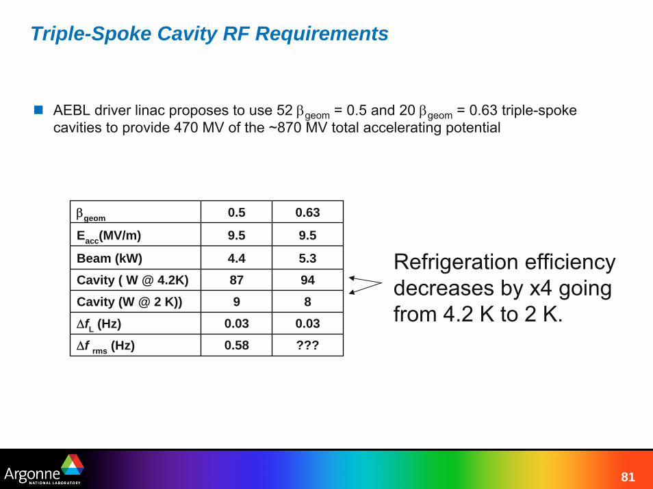
Triple-Spoke Cavity RF Requirements
AEBL driver linac proposes to use 52 βgeom = 0.5 and 20 βgeom = 0.63 triple-spoke cavities to provide 470 MV of the ~870 MV total accelerating potential
βgeom 0.5 0.63
Eacc(MV/m) 9.5 9.5
Beam (kW) 4.4 5.3Cavity ( W @ 4.2K) 87 94Cavity (W @ 2 K)) 9 8ΔfL (Hz) 0.03 0.03Δf rms (Hz) 0.58 ???
Refrigeration efficiencydecreases by x4 goingfrom 4.2 K to 2 K.
82
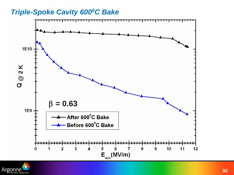
Triple-Spoke Cavity 6000C Bake
β = 0.63
@ 2
K
83
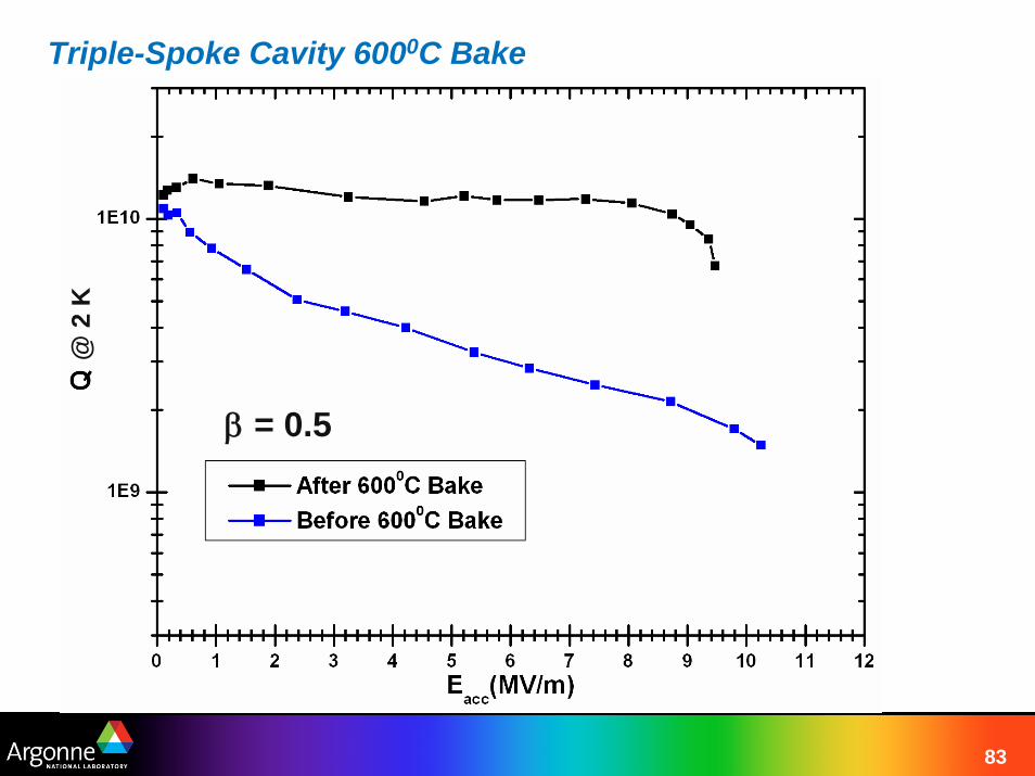
Triple-Spoke Cavity 6000C Bake
β = 0.5
@ 2
K

84
Triple-Spoke Cavity 6000C Bake@
2 K
85
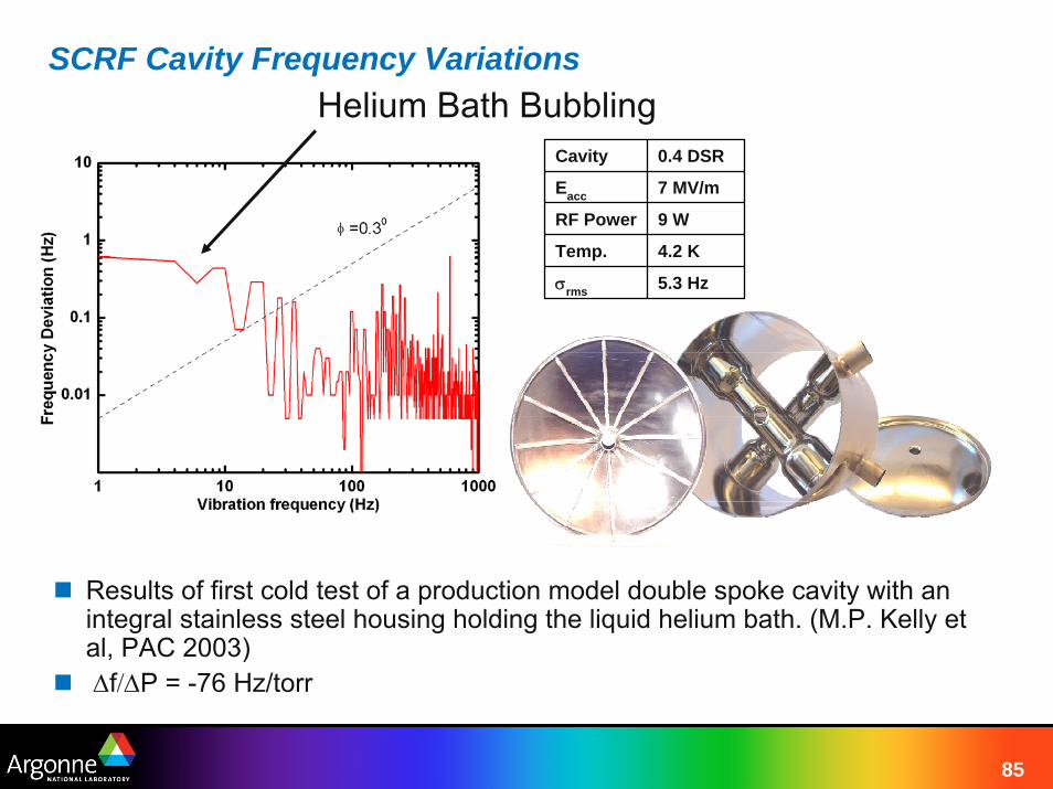
SCRF Cavity Frequency Variations
Results of first cold test of a production model double spoke cavity with an integral stainless steel housing holding the liquid helium bath. (M.P. Kelly et al, PAC 2003)Δf/ΔP = -76 Hz/torr
Cavity 0.4 DSR
Eacc 7 MV/m
RF Power 9 W
Temp. 4.2 K
σrms 5.3 Hz
Helium Bath Bubbling
86
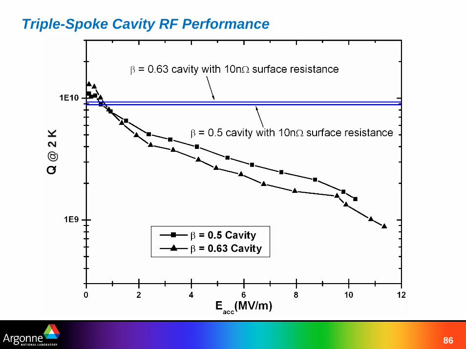
Triple-Spoke Cavity RF Performance
@ 2
K
87
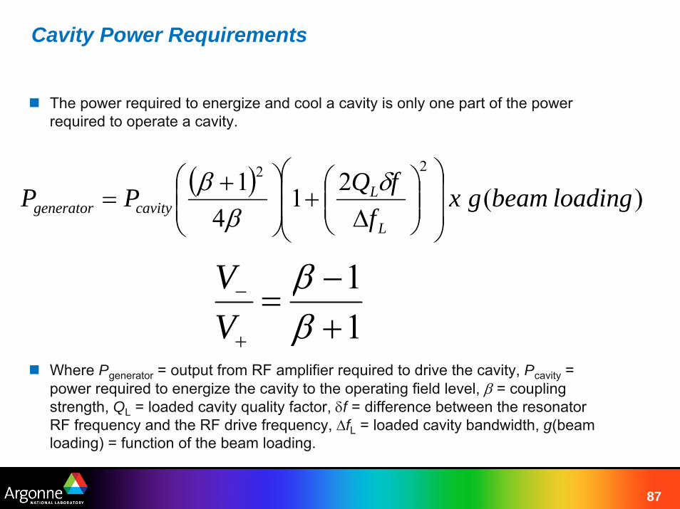
Cavity Power Requirements
The power required to energize and cool a cavity is only one part of the power required to operate a cavity.
( ) )(214
122
loadingbeamgxf
fQPPL
Lcavitygenerator ⎟
⎟
⎠
⎞
⎜⎜
⎝
⎛⎟⎟⎠
⎞⎜⎜⎝
⎛Δ
+⎟⎟⎠
⎞⎜⎜⎝
⎛ +=
δβ
β
Where Pgenerator = output from RF amplifier required to drive the cavity, Pcavity = power required to energize the cavity to the operating field level, β = coupling strength, QL = loaded cavity quality factor, δf = difference between the resonator RF frequency and the RF drive frequency, ΔfL = loaded cavity bandwidth, g(beamloading) = function of the beam loading.
11
+−
=+
−
ββ
VV

88
SCRF Cavity Frequency Variations
βgeo = 0.5 Triple-Spoke-Loaded Cavity
Frequency 345.23 MHz
βgeom 0.5
L(3βλ/2) 65.2 cm
QRs (G) 88.5 Ω
R/Q 492 Ω
below for EACC = 1.0 MV/m
RF Energy 0.398 j
BPEAK 86 G
EPEAK 2.79
89
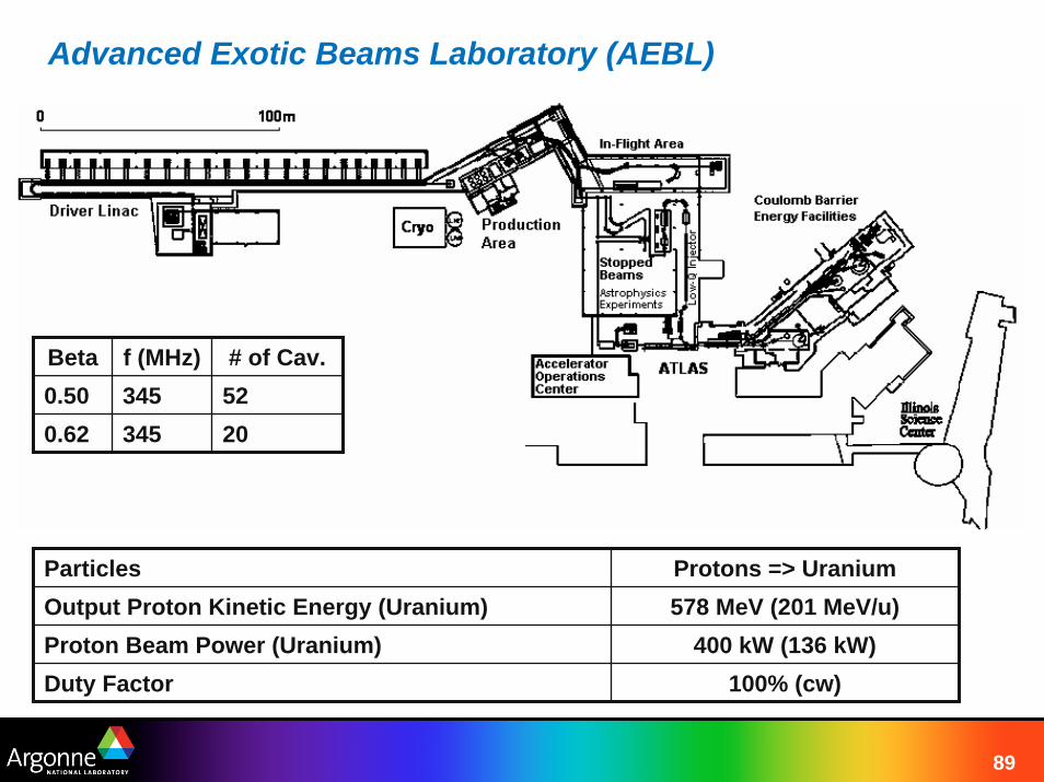
Advanced Exotic Beams Laboratory (AEBL)
Particles Protons => UraniumOutput Proton Kinetic Energy (Uranium) 578 MeV (201 MeV/u)Proton Beam Power (Uranium) 400 kW (136 kW)Duty Factor 100% (cw)
Beta f (MHz) # of Cav.0.50 345 520.62 345 20
90
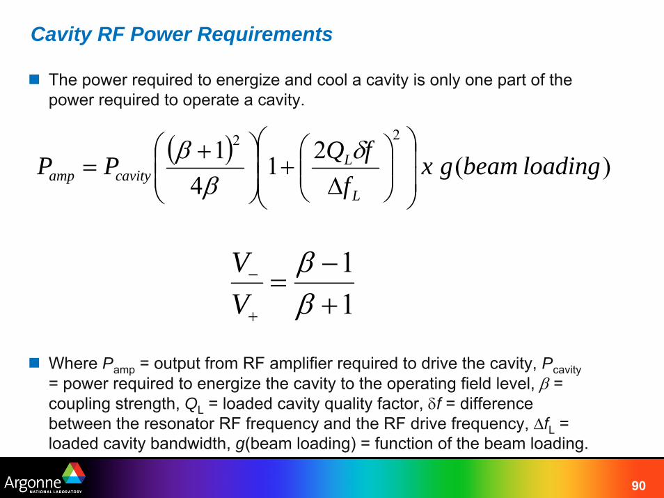
Cavity RF Power Requirements
The power required to energize and cool a cavity is only one part of the power required to operate a cavity.
( ) )(214
122
loadingbeamgxf
fQPPL
Lcavityamp ⎟
⎟
⎠
⎞
⎜⎜
⎝
⎛⎟⎟⎠
⎞⎜⎜⎝
⎛Δ
+⎟⎟⎠
⎞⎜⎜⎝
⎛ +=
δβ
β
Where Pamp = output from RF amplifier required to drive the cavity, Pcavity= power required to energize the cavity to the operating field level, β = coupling strength, QL = loaded cavity quality factor, δf = difference between the resonator RF frequency and the RF drive frequency, ΔfL = loaded cavity bandwidth, g(beam loading) = function of the beam loading.
11
+−
=+
−
ββ
VV

![1.1 The Advanced Superconducting Test …lss.fnal.gov/archive/2014/pub/fermilab-pub-14-285-ad-apc.pdf1.1 The Advanced Superconducting Test Accelerator (ASTA) at Fermilab [] Elvin Harms,](https://img.dokumen.tips/doc/110x75/5b065e3d7f8b9a58148cbdf3/11-the-advanced-superconducting-test-lssfnalgovarchive2014pubfermilab-pub-14-285-ad-apcpdf11.jpg)