Project planning with alternative technologies in

doi:10.1016/j.ejor.2014.11.014 • www.stefancreemers.be • [email protected]

Project planning with alternative technologies in

uncertain environments

Stefan CreemersBert De Reyck

Roel Leus

Abstract - We investigate project scheduling with stochastic activity durationsto maximize the expected net present value. Individual activities also carry arisk of failure, which can cause the overall project to fail. In the project planningliterature, such technological uncertainty is typically ignored and project plansare developed only for scenarios in which the project succeeds. To mitigatethe risk that an activity’s failure jeopardizes the entire project, more than onealternative may exist for reaching the project’s objectives. We propose a modelthat incorporates both the risk of activity failure and the possible pursuit ofalternative technologies. We find optimal solutions to the scheduling problemby means of stochastic dynamic programming. Our algorithms prescribe whichalternatives need to be explored, and how they should be scheduled. We alsoexamine the impact of the variability of the activity durations on the project’svalue.

Keywords - project scheduling, uncertainty, net present value, alternative tech-nologies, stochastic activity durations

1 Introduction

Projects in many industries are subject to considerable uncertainty, due to many possiblecauses. Factors influencing the completion date of a project include activities that arerequired but that were not identified beforehand, activities taking longer than expected,activities that need to be redone, resources being unavailable when required, late deliveries,etc. In research and development (R&D) projects, there is also the risk that activities mayfail altogether, requiring the project to be halted completely. This risk is often referred toas technical risk. In this text, we focus on two main sources of uncertainty in R&D projects,namely uncertain activity durations and the possibility of activity failure: we incorporatethe concept of activity success or failure into the analysis of projects with stochastic activitydurations, where the successful completion of an activity can correspond to a technologicaldiscovery or scientific breakthrough. We examine the impact of these two factors on optimalplanning strategies that maximize the project’s value, and on its value itself.

This work is a continuation of De Reyck and Leus [12], where an algorithm is developedfor project scheduling with uncertain activity outcomes and where project success is achievedonly if all individual activities succeed. Reference [12] constituted the first description of anoptimal approach for handling activity failures in project scheduling, but neither stochastic

1

http://dx.doi.org/10.1016/j.ejor.2014.11.014

http://www.stefancreemers.be

mailto:[email protected]


activity durations nor the possibility of pursuing multiple alternatives for the same result,and the inherent possibility of activity selection, were accounted for. Earlier work studiedoptimal procedures for special cases; see Chun [8], for instance. Other references relevant tothis text stem from the discipline of chemical engineering, mainly the work by Grossmannand his colleagues (e.g., [33, 21]), who studied the scheduling of failure-prone new-productdevelopment (NPD) testing tasks when non-sequential testing is admitted. They point outthat in industries such as chemicals and pharmaceuticals, the failure of a single required en-vironmental or safety test may prevent a potential product from reaching the marketplace,which has inspired our modeling of possible activity and project failure. Therefore, our mod-els are also of particular interest to drug-development projects, in which stringent scientificprocedures have to be followed in distinct stages to ensure patient safety, before a medicinecan be approved for production. Such projects may need to be terminated in any of thesestages, either because the product is revealed not to have the desired properties or becauseof harmful side effects. Illustrations of modeling pharmaceutical projects, with a focus onresource allocation, can be found in Gittins and Yu [16] and Yu and Gittins [39].

Due to the risk of activity failure resulting in overall project failure, it has been suggestedthat R&D projects should explore multiple alternative ways for developing new products(Sommer and Loch [35]). To mitigate the risk that an individual activity’s failure jeopar-dizes the entire project, we model projects in which the same (intermediate or final) outcomecan be pursued in several different ways, where one success allows the project to continue.The different attempts can be multiple trials of the same procedure or the pursuit of differentalternative ways to achieve the same outcome, e.g., the exploration of alternative technolo-gies. Following Baldwin and Clark [3], a unit of alternative interdependent tasks with adistinguished deliverable will be called a module.

Project profitability is often measured by the project’s net present value (NPV), thediscounted value of the project’s cash flows. This NPV is affected by the project scheduleand therefore, the timing of expenditures and cash inflows has a major impact on the project’sfinancial performance, especially in capital-intensive industries. The goal of this article is tofind optimal scheduling strategies that maximize the expected NPV (eNPV) of the projectwhile taking into account the activity costs, the cash flows generated by a successful project,the variability in the activity durations, the precedence constraints, the likelihood of activityfailure and the option to pursue multiple trials or technologies. Thus, this article extends thework of Buss and Rosenblatt [6], Benati [5], Sobel et al. [34] and Creemers et al. [10], whofocus on duration risk only, and of Schmidt and Grossmann [33], Jain and Grossmann [21] andDe Reyck and Leus [12], who look into technical risk only (although Schmidt and Grossmann[33] also explore the possibility of introducing multiple discrete duration scenarios).

Our contributions are fourfold: (1) we introduce and formulate a generic model for op-timal scheduling of R&D activities with stochastic durations, non-zero failure probabilitiesand modular completion subject to precedence constraints; to the best of knowledge, sucha model has never been studied before; (2) we develop a dynamic-programming recursionto determine an optimal policy for executing the project while maximizing the project’seNPV, extending the algorithm of Creemers et al. [10] with activity failures, multiple trialsand phase-type (PH) distributed activity durations instead of exponentials; (3) we conductnumerical experiments to demonstrate the computational capabilities of the algorithm; and(4) we examine the impact of activity duration risk on the optimal scheduling policy and

2





project values. Interestingly, our findings indicate that higher operational variability doesnot always lead to lower project values, meaning that (sometimes costly) variance reductionstrategies are not always advisable. To the best of our knowledge, this is the first article tonumerically support such a recommendation.

The remainder of this text is organized as follows. In Section 2, we provide the necessarydefinitions and a detailed problem statement. We produce solutions by means of a backwarddynamic-programming recursion for a Markov decision process, which is discussed in Sec-tion 3. Section 4 reports on our computational performance on a representative set of testinstances. In Section 5, a computational experiment is described in which we examine theeffect of activity duration variability on the eNPV of a project and Section 6 evaluates twodifferent choices for the policy class to be considered. Section 7 contains a brief summary ofthe text.

2 Definitions and problem statement

2.1 Stochastic project scheduling

A project consists of a set of activities N = {0, . . . , n}. The execution of a project withstochastic components (in our case, stochastic activity outcomes and durations) is a dynamicdecision process. A solution, therefore, cannot be represented by a schedule but takes theform of a policy : a set of decision rules defining actions at decision times, which maydepend on the prior outcomes. Decision times are typically the start of the project andthe completion times of activities; a tentative next decision time can also be specified bythe decision maker. An action entails the start of a precedence-feasible set of activities(see Section 2.2 for a statement of the precedence constraints). In this way, a schedule isconstructed gradually as time progresses. Next to the information available at the start of theproject, a decision at time t can only use information on duration realizations and activityoutcomes that has become available before or at time t; this is the so-called non-anticipativityconstraint. Activities should be executed without interruption.

Each activity i ∈ N\{n} has a probability of technical success pi; we assume that p0 = 1.We do not consider (renewable or other) resource constraints and assume the outcomes ofthe different tasks to be independent. We define a success (state) vector as an n-componentbinary vector x = (x0, x1, . . . , xn−1), with one component associated with each activity inN \ {n}. We let Xi represent the Bernoulli random variable with parameter pi as successprobability for each activity i, and we write X = (X0, X1, . . . , Xn−1). Information on anactivity’s success (the realization of Xi) becomes available only at the end of that activity.We say that x is a realization or scenario of X. The duration Dj ≥ 0 of each activity j is alsoa stochastic variable; the vector (D0, D1, . . . , , Dn) is denoted by D. We use lowercase vectord = (d0, . . . , , dn) to represent one particular realization of D, and we assume Pr[D0 = 0] =Pr[Dn = 0] = 1.

We assume that all activity cash flows during the development phase are non-positive,which is typical for R&D projects: the (known) cash flow associated with the executionof activity i ∈ N\{n} is represented by the integer value ci ≤ 0 and is incurred at thestart of the activity. We choose c0 = 0. If the project is successful (see Section 2.2 for the

3





specific conditions under which this is true) then the final activity n can be executed. Thiscorresponds with obtaining an end-of-project payoff C ≥ 0, which is received at the startof activity n (which is also its completion time). The value si ≥ 0 represents the startingtime of activity i; we call the (n + 1)-vector s = (s0, s1, . . . , sn) a schedule, with si ≥ 0 forall i ∈ N . We assume s0 = 0 in what follows: the project starts at time zero. The valuesi = +∞ means that activity i will not be executed at all.

We follow Igelmund and Radermacher [20], Mohring [27] and Stork [36], who study projectscheduling with resource constraints and stochastic activity durations, in interpreting everyscheduling policy Π as a function Rn−1

≥ × Bn → Rn+1≥ , with R≥ the set of non-negative

reals and B = {0, 1}. The function Π maps given samples (d,x) of activity durations andsuccess vectors to vectors s(d,x; Π) of feasible activity starting times (schedules). For agiven duration scenario d, success vector x and policy Π, sn(d,x; Π) denotes the makespanof the schedule, which coincides with project completion. Note that not all activities need tobe completed (or even started) by sn, nor that the realization of all Xi’s needs to be known.

We compute the NPV for schedule s as

f(s) = Ce−rsn +n−1∑i=1si 6=∞

cie−rsi , (1)

with r a continuous discount rate chosen to represent the time value of money: the presentvalue of a cash flow c incurred at time t equals ce−rt, where e is the base of the naturallogarithm. Our goal in this article is to select a policy Π∗ that maximizes E[f(s(D,X; Π))],with E[·] the expectation operator with respect to D and X; we write E[f(Π)], for short.The generality of this problem statement suggests that optimization over the class of allpolicies is probably computationally impractical. We therefore restrict our optimization to asubclass that has a simple combinatorial representation and where decision points are limitedin number: our solution space P consists of all policies that start activities only at the endof other activities (activity 0 is started at time 0). The solution space also contains policyΠ0, which corresponds with immediate abandonment of the project (formally, all startingtimes apart from s0 are set to infinity), which will be preferable when C is not large enoughcompared to the costs of the activities: then it is better simply not to undertake the projectat all, with objective value 0.

2.2 Modular projects

Modularity means splitting the design and production of technologies into independent sub-parts [3]. This has benefits towards inventory management for mass-produced items viatechniques such as commonality and postponement [7], but also with respect the durationand chances of success of a product development project by itself: in this setting, a module isa set of alternative development activities that pursue a similar target, representing repeatedtrials or technological alternatives. Lenfle [24] provides a thorough literature review of themanagement of projects via modules, and he points out that different alternatives can bepursued either in parallel or sequentially, or following a mix of both strategies. Obviously,management can also decide not to pursue certain alternatives, for instance because theircost is too high compared to their expected benefits.

4





Lenfle refers to the Manhattan Project as one prime example where such techniques wereapplied (for instance, multiple alternative bomb assembly designs were tested simultane-ously). Weitzman [38] brings up the evaluation and selection of alternative suppliers forsome commodity as one possible practical application. Nelson [29] cites a RAND workingpaper on the development of a new microwave relay system at Bell Telephone Laboratories,where the eventual success of the development was greatly facilitated by running multipleapproaches in parallel to solving some of the encountered development problems. Granotand Zuckerman [17] refer to the development of nylon at DuPont, where numerous poly-mers were tested one by one before the discovery of a suitable polyamide. Abernathy andRosenbloom [1] evaluate the merits of a parallel strategy at a critical point in a million-dollaradvanced power-supply development project. In the context of the development of an AIDSvaccine, Ding and Eliashberg [13] note that ‘In many new product development (NPD) situ-ations, the development process is characterized by uncertainty, and no single developmentapproach will necessarily lead to a successful product. To increase the likelihood of havingat least one successful product, multiple approaches may be simultaneously funded at thevarious NPD stages.’

In this text, we will take the modular structure of the project as given, assuming thatan appropriate project network design and initial selection of development alternatives havealready been set out. Formally, the set of modules is M = {0, . . . ,m}; each module i ∈ Mcontains the activities Ni ⊂ N , and the set of modules constitutes a partition of N : N =⋃i∈M Ni and Ni ∩ Nj = ∅ if i 6= j. A is a (strict) partial order on M , i.e., an irreflexive

and transitive relation, which represents technological precedence constraints. (Dummy)modules 0 and m represent the start and the end of the project, respectively; they are the(unique) least and greatest element of the partially ordered set (M,A) and are assumedto contain only one (dummy) activity, indexed by 0 and n, respectively. On the activitieswithin each module i, we also impose a partial order Bi, to allow for modeling precedencerequirements between these activities. In drug development, for example, when a certainmodule is needed to show the effectiveness of a drug, two precedence-related activities couldrepresent the repeated measurement of the beneficial effects of the drug: the first test isperformed after one week; the effects after two weeks will only be measured if first theeffects after one week are inconclusive [9]. Alternatively, trials may be repeated in differentdoses and with different test subjects [19]. Precedence constraints within modules may alsorepresent fallback options for project failure, as ‘contingency plans’: plans devised for anoutcome different from expected. Comparable modeling choices were made in Coolen etal. [9] and in Huysmans et al. [19], but without discounting the cash flows, in which casedurations become irrelevant and scheduling all activities sequentially is a dominant choice.

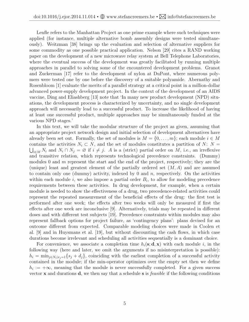
For convenience, we associate a completion time hi(s; d,x) with each module i, in thefollowing way (here and later, we omit the arguments if no misinterpretation is possible):hi = minj∈Ni|xj=1{sj + dj}, coinciding with the earliest completion of a successful activitycontained in the module; if the min-operator optimizes over the empty set then we definehi := +∞, meaning that the module is never successfully completed. For a given successvector x and durations d, we then say that a schedule s is feasible if the following conditions

5





are fulfilled:

hi ≤ sj ∀(i, k) ∈ A,∀j ∈ Nk (2)

si + di ≤ sj ∀k ∈M,∀(i, j) ∈ Bk (3)

Equations (2) are inter-module precedence constraints, which imply that a necessary condi-tion for the start of an activity j ∈ Nk is success for all the predecessor modules i of themodule k to which j belongs, where a module is said to be successful if at least one of itsconstituent activities succeeds. Equations (3) are intra-module constraints: an activity j canonly be started when all predecessor activities i in the same module have been completed,and its execution would obviously be useful only if all those predecessors failed. An activity’sstarting time equal to infinity corresponds to not executing the activity and therefore notincurring any related expenses, or in case of activity n, not receiving the project payoff.Consequently, the project payoff is achieved (sn 6=∞) only if every module is successful.

The classic PERT problem [2, 14, 23, 26] aims at characterizing the random variablesn(D,1; ΠES), where policy ΠES starts all activities as early as possible, each module containsonly one activity, and 1 is an n-vector with value 1 in all components. Contrary to themakespan, however, NPV is a non-regular measure of performance: starting activities asearly as possible is not necessarily optimal, since the ci are usually negative.

2.3 Illustration

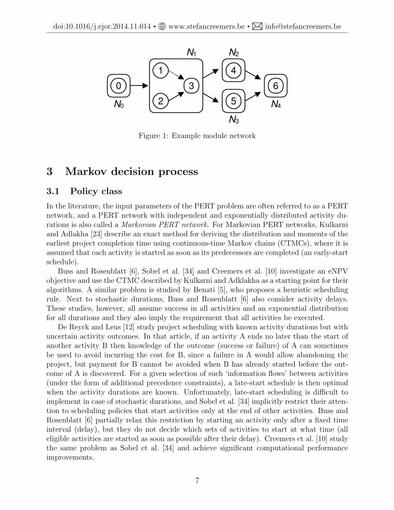
Figure 1 illustrates the foregoing definitions and problem statement. This project consistsof seven activities, N = {0, 1, 2, 3, 4, 5, 6}, where 0 and n = 6 are dummies. There are fivemodules, so m = 4 : N0 = {0} , N1 = {1, 2, 3} , N2 = {4}, N3 = {5} and N4 = {6}. In theexample, B1 = {(1, 3), (2, 3)}. Note that Figure 1 actually shows the transitive reductionof A: the order relation A also contains elements such as (0, 2) and (1, 4), while the arcsN0 → N2 and N1 → N4 are not included in the figure.

A policy Π12 for this project is the following: start the project at time 0 (s0 = 0) andimmediately initiate activities 1 and 2 (s1 = s2 = 0). If X1 = X2 = 0 then abandon theproject: set s3 = s4 = s5 = s6 = +∞. Otherwise, module N1 completes successfully. Inthat case, start both activities 4 and 5 upon the successful completion of activity 1 or 2(whichever is the earliest), and terminate the project if either 4 or 5 fails. Note that underpolicy Π12, activity 3 is never started, and we effectively include activity selection as part ofthe decisions to be made. Represented as a function, Π12 entails the following mapping:

(d1, d2, d3, d4, d5, x0, x1, x2, x3, x4, x5)7→

(0, 0, 0,∞, h1, h1,max{h2;h3}),

with h1 = minj=1,2;xj=1{dj} and h1 =∞ if x1 = x2 = 0, h2 = h1 + d4 if x4 = 1 and h2 =∞if x4 = 0, and h3 = h1 + d5 if x5 = 1 and h3 =∞ if x5 = 0.

6





N0

4

N1 N2

N3

N4

6

5

0

1

2

3

Figure 1: Example module network

3 Markov decision process

3.1 Policy class

In the literature, the input parameters of the PERT problem are often referred to as a PERTnetwork, and a PERT network with independent and exponentially distributed activity du-rations is also called a Markovian PERT network. For Markovian PERT networks, Kulkarniand Adlakha [23] describe an exact method for deriving the distribution and moments of theearliest project completion time using continuous-time Markov chains (CTMCs), where it isassumed that each activity is started as soon as its predecessors are completed (an early-startschedule).

Buss and Rosenblatt [6], Sobel et al. [34] and Creemers et al. [10] investigate an eNPVobjective and use the CTMC described by Kulkarni and Adklakha as a starting point for theiralgorithms. A similar problem is studied by Benati [5], who proposes a heuristic schedulingrule. Next to stochastic durations, Buss and Rosenblatt [6] also consider activity delays.These studies, however, all assume success in all activities and an exponential distributionfor all durations and they also imply the requirement that all activities be executed.

De Reyck and Leus [12] study project scheduling with known activity durations but withuncertain activity outcomes. In that article, if an activity A ends no later than the start ofanother activity B then knowledge of the outcome (success or failure) of A can sometimesbe used to avoid incurring the cost for B, since a failure in A would allow abandoning theproject, but payment for B cannot be avoided when B has already started before the out-come of A is discovered. For a given selection of such ‘information flows’ between activities(under the form of additional precedence constraints), a late-start schedule is then optimalwhen the activity durations are known. Unfortunately, late-start scheduling is difficult toimplement in case of stochastic durations, and Sobel et al. [34] implicitly restrict their atten-tion to scheduling policies that start activities only at the end of other activities. Buss andRosenblatt [6] partially relax this restriction by starting an activity only after a fixed timeinterval (delay), but they do not decide which sets of activities to start at what time (alleligible activities are started as soon as possible after their delay). Creemers et al. [10] studythe same problem as Sobel et al. [34] and achieve significant computational performanceimprovements.

7





In this article, we also propose to restrict the attention to policies that start activities atthe completion time of other activities. This can be seen to be a dominant set of policies forthose cases in which the project payoff is sufficiently large relative to the costs associatedwith the intermediate activities, because the benefit of delaying the payment of an activitywould then be more than offset by the disadvantage of the higher possibility of delay inobtaining the payoff; this reasoning holds for any discount rate r > 0. The generalization inwhich activity starting times are delayed by a fixed offset beyond their earliest starting timeposes significant computational challenges (cf. [6]). The models and algorithms in this articlecan be extended so that activities can also be started when other activities are ‘underway,’and in Section 6, we describe our findings for an experiment where we consider the possiblestart of new activities after each phase in the PH distribution of each ongoing activity (asetting that gives rise to a larger policy class, hence a larger search space). The experimentindicates that the average improvement in the objective function is minor (up to 0.3% of thepayoff at most, depending on the settings). We recognize that the practical relevance of thislarger policy class can obviously be questioned, and the experiment should merely be seen asan approximation of the setting where activities can be started whenever the decision makerchooses. We conclude that only starting activities at the completion time of other activitiesis not a very restrictive decision, under the settings tested.

Below, we extend the work of Creemers et al. [10] to accommodate PH-distributed activitydurations, possible activity failures and a modular project network, allowing also for activityselection. We first study the special case of exponential activity durations (Section 3.2),followed by an illustration (Section 3.3) and by a treatment of more general distributions(Section 3.4).

3.2 The exponential case

For the moment, we assume each duration Di to be exponentially distributed with rateparameter λi = 1/E[Di] (i = 1, . . . , n− 1); we consider more general distributions in Section3.4. At any time instant t, an activity’s status is either idle (not yet started), active (beingexecuted), or past (successfully finished, failed, or considered redundant because its moduleis completed). Let I(t), Y (t) and P (t) represent the activities in N that are idle, active andpast, respectively; these three sets are mutually exclusive and I(t) ∪ Y (t) ∪ P (t) = N . Thestate of the system is defined by the status of the individual activities and is representedby a triplet (I, Y, P ). State transitions take place each time an activity becomes past andare determined by the policy at hand. The project’s starting conditions are Y (0) = {0} andI(0) = N \ {0}, while the condition for successful completion of the project is P (t∗) = N ,where t∗ represents the project completion time.

The problem of finding an optimal scheduling policy corresponds to optimizing a dis-counted criterion in a continuous-time Markov decision chain (CTMDC) on the state spaceQ, with Q containing all the states of the system that can be visited by the transitions(which are called feasible states); the decision set is described below. We apply a backwardstochastic dynamic-programming (SDP) recursion to determine optimal decisions based onthe CTMC described in Kulkarni and Adlakha [23]. The key instrument of the SDP recur-sion is the value function F (·), which determines the expected NPV of each feasible state atthe time of entry of the state, conditional on the hypothesis that optimal decisions are made

8





in all subsequent states and assuming that all ‘past’ modules (with all activities past) weresuccessful. In the definition of the value function F (I, Y ), we supply sets I and Y of idleand active activities as parameters (which uniquely determines the past activities). Whenan activity finishes, three different state transitions can occur: (1) activity j ∈ Ni completessuccessfully; (2) activity j ∈ Ni fails and another activity k ∈ Ni is still idle or active; (3)activity j ∈ Ni fails and all other activities k ∈ Ni have already failed (or it is the onlyactivity in the module).

We define the order B∗ on set N to relate activities that do not necessarily belong to thesame module, as follows:

(i, j) ∈ B∗ ⇔ (∃Bm : (i, j) ∈ Bm) ∨ (∃(l,m) ∈ A : i ∈ Nl ∧ j ∈ Nm).

We call an activity j eligible at time t if j ∈ I(t) and ∀(k, j) ∈ B∗ : k ∈ P (t). LetE(I, Y ) ⊂ N be the set of eligible activities for given sets I and Y of idle and activeactivities. Upon entry of a state (I, Y, P ) ∈ Q, a decision needs to be made whether or notto start eligible activities in E(I, Y ) and if so, which. If no activities are started, a transitiontowards another state occurs at the first completion of an element of Y . Not starting anyactivities while there are no active activities left, corresponds to abandoning the project.Let λ =

∑k∈Y λk. The probability that activity j ∈ Y completes first among the active

activities equals λj/λ (competing expontials; see our working paper [11] for more details).

The expected time to the first completion is λ−1 time units (the length of this timespan isalso exponentially distributed) and the appropriate discount factor to be applied for this

timespan is λ/(r + λ

)(see working paper). In state (I, Y, P ) ∈ Q, the expected NPV to be

obtained from the next state on condition that no new activities are started equals

F0(I, Y ) =λ

r + λ

∑j∈Y

pjλj

λF (I \Ni, Y \Ni)+

λ

r + λ

∑j∈Y :Ni\{j}6⊂P

(1− pj)λjλ

F (I, Y \ {j}),(4)

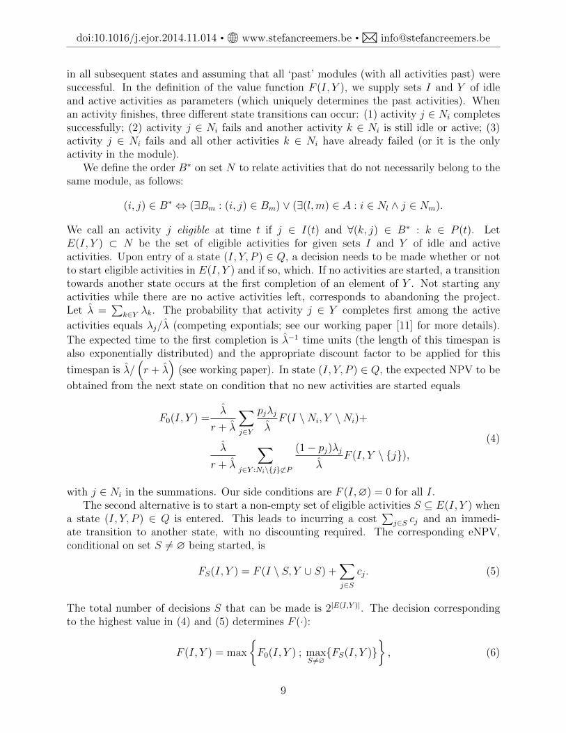
with j ∈ Ni in the summations. Our side conditions are F (I,∅) = 0 for all I.The second alternative is to start a non-empty set of eligible activities S ⊆ E(I, Y ) when

a state (I, Y, P ) ∈ Q is entered. This leads to incurring a cost∑

j∈S cj and an immedi-ate transition to another state, with no discounting required. The corresponding eNPV,conditional on set S 6= ∅ being started, is

FS(I, Y ) = F (I \ S, Y ∪ S) +∑j∈S

cj. (5)

The total number of decisions S that can be made is 2|E(I,Y )|. The decision correspondingto the highest value in (4) and (5) determines F (·):

F (I, Y ) = max

{F0(I, Y ) ; max

S 6=∅{FS(I, Y )}

}, (6)

9





for feasible state (I, Y,N \ (I ∪ Y )).The computation of the backward SDP recursion (6) starts in state (∅, {n}, N \ {n}).

Subsequently, the value function is evaluated stepwise for all other states. The optimalobjective value maxΠ∈P E[f(Π)] is obtained as F (N \ {0}, {0}). We should note that thepolicies from which one with the best objective function is chosen, do not consider the optionof starting activities at the end of activities that are redundant (past) because anotheractivity already made their module succeed.

3.3 Illustration

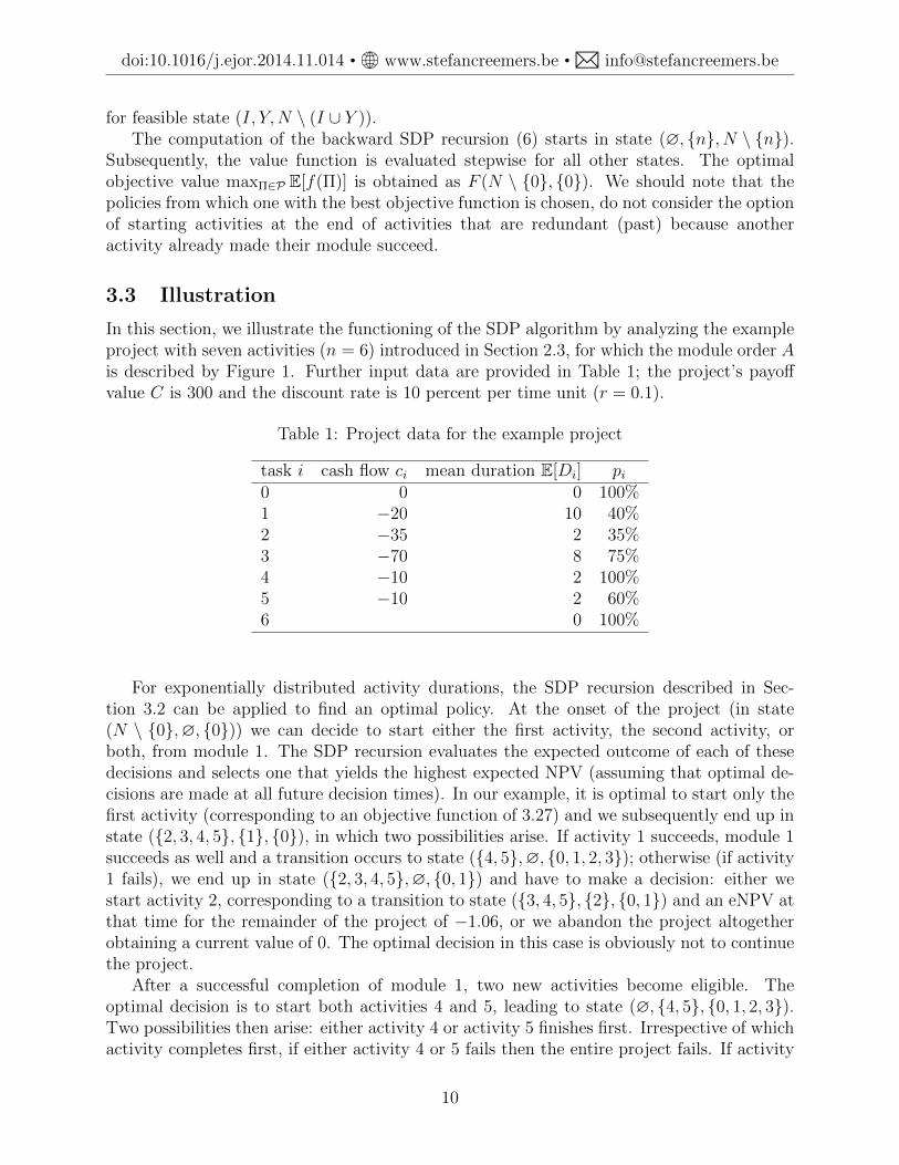
In this section, we illustrate the functioning of the SDP algorithm by analyzing the exampleproject with seven activities (n = 6) introduced in Section 2.3, for which the module order Ais described by Figure 1. Further input data are provided in Table 1; the project’s payoffvalue C is 300 and the discount rate is 10 percent per time unit (r = 0.1).

Table 1: Project data for the example project

task i cash flow ci mean duration E[Di] pi0 0 0 100%1 −20 10 40%2 −35 2 35%3 −70 8 75%4 −10 2 100%5 −10 2 60%6 0 100%

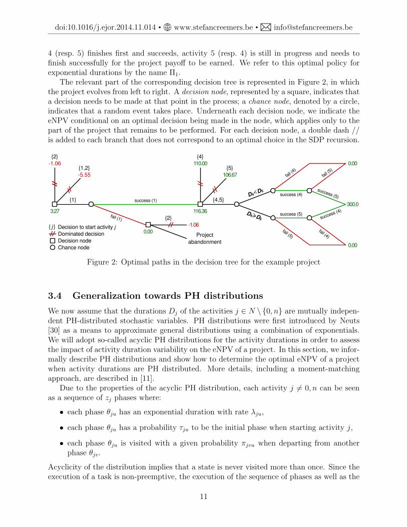
For exponentially distributed activity durations, the SDP recursion described in Sec-tion 3.2 can be applied to find an optimal policy. At the onset of the project (in state(N \ {0},∅, {0})) we can decide to start either the first activity, the second activity, orboth, from module 1. The SDP recursion evaluates the expected outcome of each of thesedecisions and selects one that yields the highest expected NPV (assuming that optimal de-cisions are made at all future decision times). In our example, it is optimal to start only thefirst activity (corresponding to an objective function of 3.27) and we subsequently end up instate ({2, 3, 4, 5}, {1}, {0}), in which two possibilities arise. If activity 1 succeeds, module 1succeeds as well and a transition occurs to state ({4, 5},∅, {0, 1, 2, 3}); otherwise (if activity1 fails), we end up in state ({2, 3, 4, 5},∅, {0, 1}) and have to make a decision: either westart activity 2, corresponding to a transition to state ({3, 4, 5}, {2}, {0, 1}) and an eNPV atthat time for the remainder of the project of −1.06, or we abandon the project altogetherobtaining a current value of 0. The optimal decision in this case is obviously not to continuethe project.

After a successful completion of module 1, two new activities become eligible. Theoptimal decision is to start both activities 4 and 5, leading to state (∅, {4, 5}, {0, 1, 2, 3}).Two possibilities then arise: either activity 4 or activity 5 finishes first. Irrespective of whichactivity completes first, if either activity 4 or 5 fails then the entire project fails. If activity

10





4 (resp. 5) finishes first and succeeds, activity 5 (resp. 4) is still in progress and needs tofinish successfully for the project payoff to be earned. We refer to this optimal policy forexponential durations by the name Π1.

The relevant part of the corresponding decision tree is represented in Figure 2, in whichthe project evolves from left to right. A decision node, represented by a square, indicates thata decision needs to be made at that point in the process; a chance node, denoted by a circle,indicates that a random event takes place. Underneath each decision node, we indicate theeNPV conditional on an optimal decision being made in the node, which applies only to thepart of the project that remains to be performed. For each decision node, a double dash //is added to each branch that does not correspond to an optimal choice in the SDP recursion.

-1.06

-5.55

3.27

{1}

{1,2}

{2}

{2}

{4}

{4,5}

0.00

-1.06

success (1)

116.36

success (4)

success (5)

300.0

0.00

0.00

106.67

{5}110.00

success (5)

success (4)

fail (4)

fail (5)

fail (1)

Decision node

Chance node

Dominated decision

{ j } Decision to start activity j

Project

abandonment

D4>D

5

D4<D5

fail (5)

fail (4)

Figure 2: Optimal paths in the decision tree for the example project

3.4 Generalization towards PH distributions

We now assume that the durations Dj of the activities j ∈ N \ {0, n} are mutually indepen-dent PH-distributed stochastic variables. PH distributions were first introduced by Neuts[30] as a means to approximate general distributions using a combination of exponentials.We will adopt so-called acyclic PH distributions for the activity durations in order to assessthe impact of activity duration variability on the eNPV of a project. In this section, we infor-mally describe PH distributions and show how to determine the optimal eNPV of a projectwhen activity durations are PH distributed. More details, including a moment-matchingapproach, are described in [11].

Due to the properties of the acyclic PH distribution, each activity j 6= 0, n can be seenas a sequence of zj phases where:

• each phase θju has an exponential duration with rate λju,

• each phase θju has a probability τju to be the initial phase when starting activity j,

• each phase θju is visited with a given probability πjvu when departing from anotherphase θjv.

Acyclicity of the distribution implies that a state is never visited more than once. Since theexecution of a task is non-preemptive, the execution of the sequence of phases as well as the

11





execution of a phase itself should be uninterrupted. Therefore, upon completion of a phaseθju:

• activity j completes with probability πju0 (absorption is reached in the underlyingMarkov chain),

• phase v is started with probability πjuv.

The exponential distribution for activity j ∈ N \{0, n} is then a PH distribution with zj = 1,τj1 = 1 and λj1 ≡ λj.

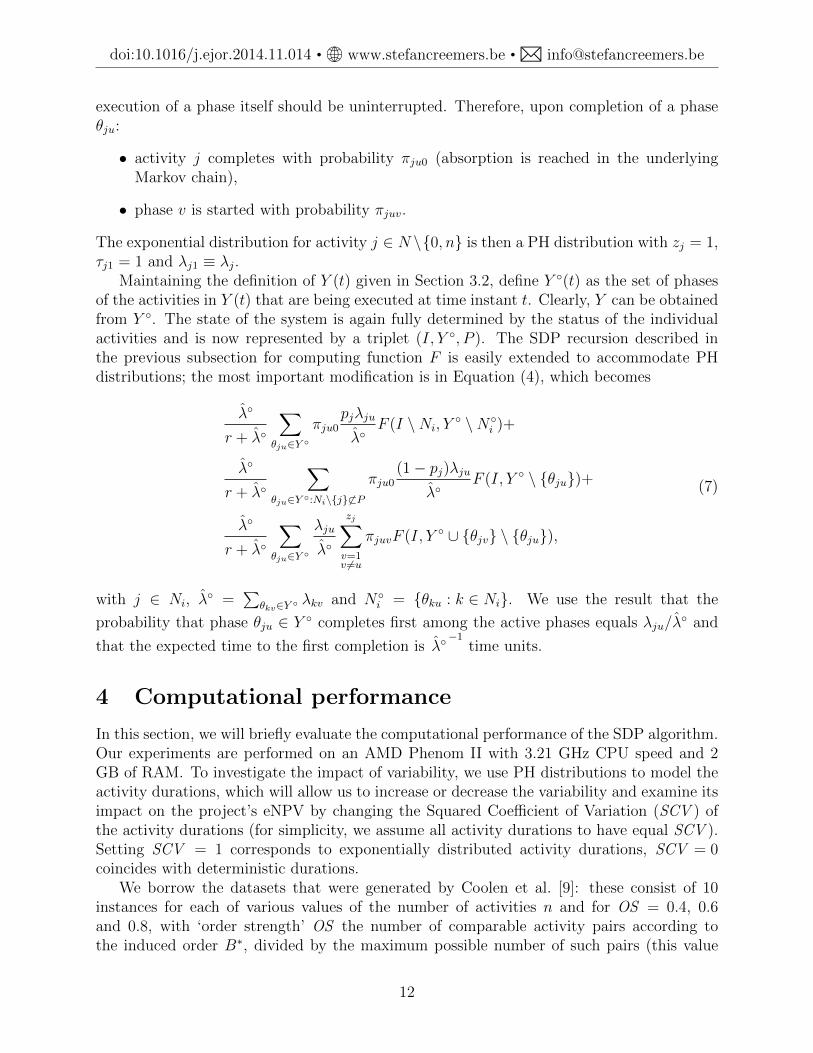
Maintaining the definition of Y (t) given in Section 3.2, define Y ◦(t) as the set of phasesof the activities in Y (t) that are being executed at time instant t. Clearly, Y can be obtainedfrom Y ◦. The state of the system is again fully determined by the status of the individualactivities and is now represented by a triplet (I, Y ◦, P ). The SDP recursion described inthe previous subsection for computing function F is easily extended to accommodate PHdistributions; the most important modification is in Equation (4), which becomes

λ◦

r + λ◦

∑θju∈Y ◦

πju0pjλju

λ◦F (I \Ni, Y

◦ \N◦i )+

λ◦

r + λ◦

∑θju∈Y ◦:Ni\{j}6⊂P

πju0(1− pj)λju

λ◦F (I, Y ◦ \ {θju})+

λ◦

r + λ◦

∑θju∈Y ◦

λju

λ◦

zj∑v=1v 6=u

πjuvF (I, Y ◦ ∪ {θjv} \ {θju}),

(7)

with j ∈ Ni, λ◦ =

∑θkv∈Y ◦ λkv and N◦i = {θku : k ∈ Ni}. We use the result that the

probability that phase θju ∈ Y ◦ completes first among the active phases equals λju/λ◦ and

that the expected time to the first completion is λ◦−1

time units.

4 Computational performance

In this section, we will briefly evaluate the computational performance of the SDP algorithm.Our experiments are performed on an AMD Phenom II with 3.21 GHz CPU speed and 2GB of RAM. To investigate the impact of variability, we use PH distributions to model theactivity durations, which will allow us to increase or decrease the variability and examine itsimpact on the project’s eNPV by changing the Squared Coefficient of Variation (SCV ) ofthe activity durations (for simplicity, we assume all activity durations to have equal SCV ).Setting SCV = 1 corresponds to exponentially distributed activity durations, SCV = 0coincides with deterministic durations.

We borrow the datasets that were generated by Coolen et al. [9]: these consist of 10instances for each of various values of the number of activities n and for OS = 0.4, 0.6and 0.8, with ‘order strength’ OS the number of comparable activity pairs according tothe induced order B∗, divided by the maximum possible number of such pairs (this value

12





is only approximate). Average activity durations are not used by Coolen et al. [9] andare additionally generated for each activity, for each instance separately; each such averageduration is a uniform integer random variate between 1 and 15. In the generated instances,all activities apart from the final one have negative cash flows and the final activity has apositive payoff (which is also significantly larger in absolute value); we refer to the appendixof [9] for more details.

For exponential durations, an upper bound on |Q| is 3n. Enumerating all these 3n statesis not recommended, as the majority of the states typically do not satisfy the precedenceconstraints. For PH durations, the bound becomes

∏j∈N 3zj . In order to minimize storage

and computational requirements, we adopt the techniques proposed by Creemers et al. [10]:as the algorithm progresses, the information on the earlier generated states will no longerbe required for further computation and therefore the memory occupied can be freed. Thisprocedure is based on a partition of Q, allowing for the necessary subsets to be generatedand deleted when appropriate.

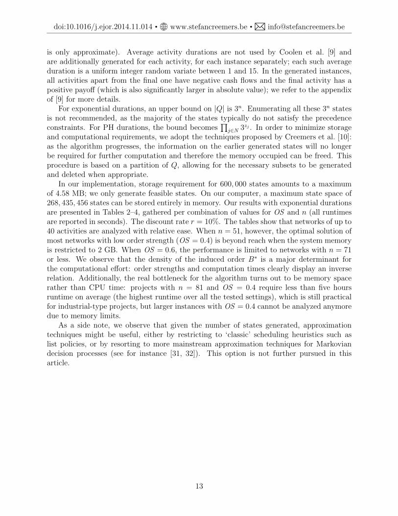
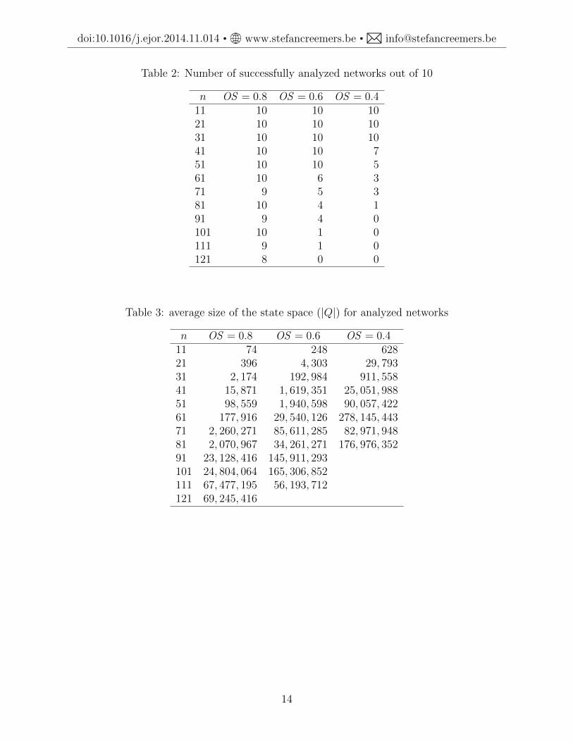
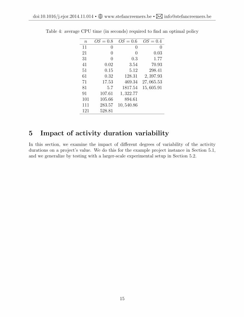
In our implementation, storage requirement for 600, 000 states amounts to a maximumof 4.58 MB; we only generate feasible states. On our computer, a maximum state space of268, 435, 456 states can be stored entirely in memory. Our results with exponential durationsare presented in Tables 2–4, gathered per combination of values for OS and n (all runtimesare reported in seconds). The discount rate r = 10%. The tables show that networks of up to40 activities are analyzed with relative ease. When n = 51, however, the optimal solution ofmost networks with low order strength (OS = 0.4) is beyond reach when the system memoryis restricted to 2 GB. When OS = 0.6, the performance is limited to networks with n = 71or less. We observe that the density of the induced order B∗ is a major determinant forthe computational effort: order strengths and computation times clearly display an inverserelation. Additionally, the real bottleneck for the algorithm turns out to be memory spacerather than CPU time: projects with n = 81 and OS = 0.4 require less than five hoursruntime on average (the highest runtime over all the tested settings), which is still practicalfor industrial-type projects, but larger instances with OS = 0.4 cannot be analyzed anymoredue to memory limits.

As a side note, we observe that given the number of states generated, approximationtechniques might be useful, either by restricting to ‘classic’ scheduling heuristics such aslist policies, or by resorting to more mainstream approximation techniques for Markoviandecision processes (see for instance [31, 32]). This option is not further pursued in thisarticle.

13





Table 2: Number of successfully analyzed networks out of 10

n OS = 0.8 OS = 0.6 OS = 0.411 10 10 1021 10 10 1031 10 10 1041 10 10 751 10 10 561 10 6 371 9 5 381 10 4 191 9 4 0101 10 1 0111 9 1 0121 8 0 0

Table 3: average size of the state space (|Q|) for analyzed networks

n OS = 0.8 OS = 0.6 OS = 0.411 74 248 62821 396 4, 303 29, 79331 2, 174 192, 984 911, 55841 15, 871 1, 619, 351 25, 051, 98851 98, 559 1, 940, 598 90, 057, 42261 177, 916 29, 540, 126 278, 145, 44371 2, 260, 271 85, 611, 285 82, 971, 94881 2, 070, 967 34, 261, 271 176, 976, 35291 23, 128, 416 145, 911, 293101 24, 804, 064 165, 306, 852111 67, 477, 195 56, 193, 712121 69, 245, 416

14





Table 4: average CPU time (in seconds) required to find an optimal policy

n OS = 0.8 OS = 0.6 OS = 0.411 0 0 021 0 0 0.0331 0 0.3 1.7741 0.02 3.54 70.9351 0.15 5.12 298.4161 0.32 128.31 2, 397.9371 17.53 469.34 27, 065.5381 5.7 1817.54 15, 605.9191 107.61 1, 322.77101 105.66 894.61111 283.57 10, 540.86121 528.81

5 Impact of activity duration variability

In this section, we examine the impact of different degrees of variability of the activitydurations on a project’s value. We do this for the example project instance in Section 5.1,and we generalize by testing with a larger-scale experimental setup in Section 5.2.

15





5.1 Impact of duration variability in the example instance

0 1 2 3 4 5 6 7 8 9 10 11 12 13 Time10

11 12 13 Time10

1-20

0Project

abandonment

300

5-10

4-10100%

60%

40%

60%

(a) Policy Π1

0 1 2 3 4 5 Time2

3 4 5 Time2

2-35

0Project

abandonment

300

5-10

4-10100%

60%

35%

65%

(b) Policy Π2

Figure 3: Policies with deterministic durations

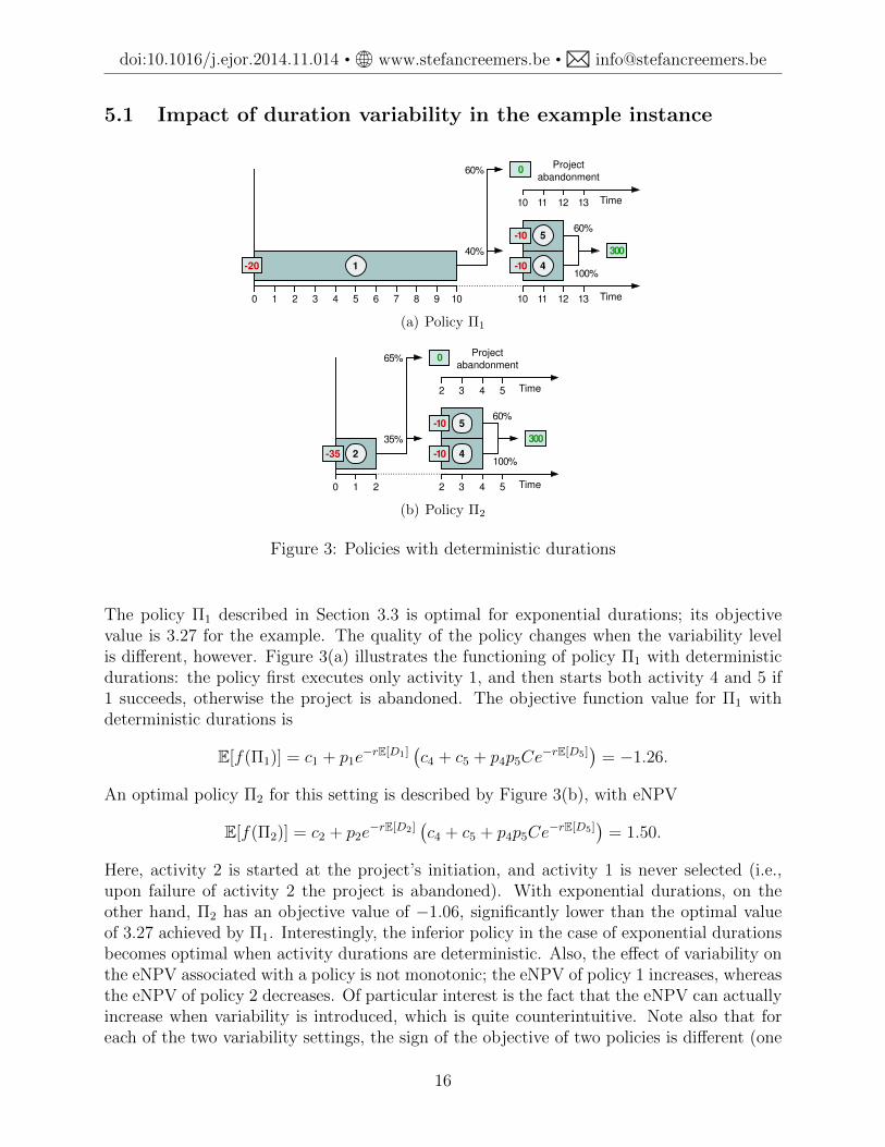
The policy Π1 described in Section 3.3 is optimal for exponential durations; its objectivevalue is 3.27 for the example. The quality of the policy changes when the variability levelis different, however. Figure 3(a) illustrates the functioning of policy Π1 with deterministicdurations: the policy first executes only activity 1, and then starts both activity 4 and 5 if1 succeeds, otherwise the project is abandoned. The objective function value for Π1 withdeterministic durations is

E[f(Π1)] = c1 + p1e−rE[D1]

(c4 + c5 + p4p5Ce

−rE[D5])

= −1.26.

An optimal policy Π2 for this setting is described by Figure 3(b), with eNPV

E[f(Π2)] = c2 + p2e−rE[D2]

(c4 + c5 + p4p5Ce

−rE[D5])

= 1.50.

Here, activity 2 is started at the project’s initiation, and activity 1 is never selected (i.e.,upon failure of activity 2 the project is abandoned). With exponential durations, on theother hand, Π2 has an objective value of −1.06, significantly lower than the optimal valueof 3.27 achieved by Π1. Interestingly, the inferior policy in the case of exponential durationsbecomes optimal when activity durations are deterministic. Also, the effect of variability onthe eNPV associated with a policy is not monotonic; the eNPV of policy 1 increases, whereasthe eNPV of policy 2 decreases. Of particular interest is the fact that the eNPV can actuallyincrease when variability is introduced, which is quite counterintuitive. Note also that foreach of the two variability settings, the sign of the objective of two policies is different (one

16





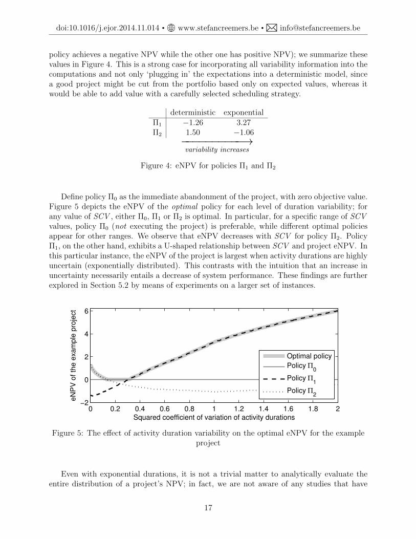
policy achieves a negative NPV while the other one has positive NPV); we summarize thesevalues in Figure 4. This is a strong case for incorporating all variability information into thecomputations and not only ‘plugging in’ the expectations into a deterministic model, sincea good project might be cut from the portfolio based only on expected values, whereas itwould be able to add value with a carefully selected scheduling strategy.

deterministic exponentialΠ1 −1.26 3.27Π2 1.50 −1.06

−−−−−−−−−−→variability increases

Figure 4: eNPV for policies Π1 and Π2

Define policy Π0 as the immediate abandonment of the project, with zero objective value.Figure 5 depicts the eNPV of the optimal policy for each level of duration variability; forany value of SCV , either Π0, Π1 or Π2 is optimal. In particular, for a specific range of SCVvalues, policy Π0 (not executing the project) is preferable, while different optimal policiesappear for other ranges. We observe that eNPV decreases with SCV for policy Π2. PolicyΠ1, on the other hand, exhibits a U-shaped relationship between SCV and project eNPV. Inthis particular instance, the eNPV of the project is largest when activity durations are highlyuncertain (exponentially distributed). This contrasts with the intuition that an increase inuncertainty necessarily entails a decrease of system performance. These findings are furtherexplored in Section 5.2 by means of experiments on a larger set of instances.

0 0.2 0.4 0.6 0.8 1 1.2 1.4 1.6 1.8 2−2

0

2

4

6

Squared coefficient of variation of activity durations

eN

PV

of th

e e

xam

ple

pro

ject

Optimal policy

Policy Π0

Policy Π1

Policy Π2

Figure 5: The effect of activity duration variability on the optimal eNPV for the exampleproject

Even with exponential durations, it is not a trivial matter to analytically evaluate theentire distribution of a project’s NPV; in fact, we are not aware of any studies that have

17





attempted to achieve this directly. More work is available on the analytical evaluation ofproject makespan in the context of the PERT problem. It turns out that, with discreteindependent durations, computing the expected makespan, and computing a single point ofthe distribution function, are both #P-complete (any #P-complete problem is polynomiallyequivalent to counting the number of Hamiltonian cycles of a graph and thus in particularNP-complete) [18, 28]. Since project NPV is a function of project makespan, this is at leastclear indication that evaluating NPV analytically is probably highly intractable for generalduration distributions, and we therefore resort to simulation as a means to approximate theNPV distribution.

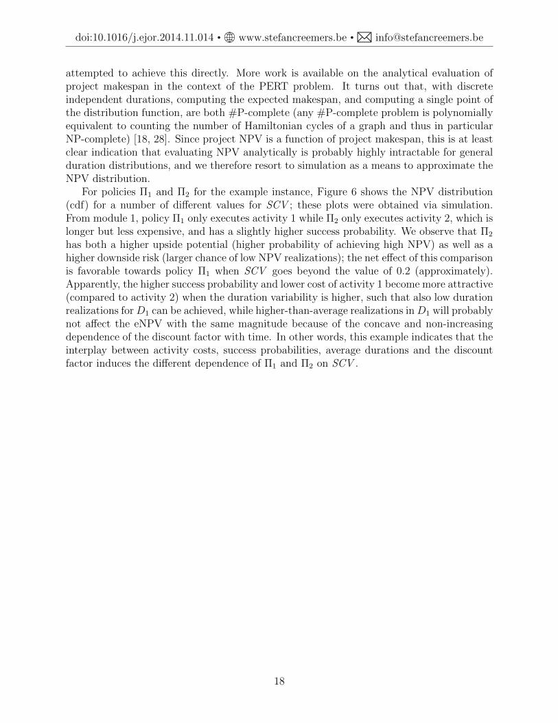
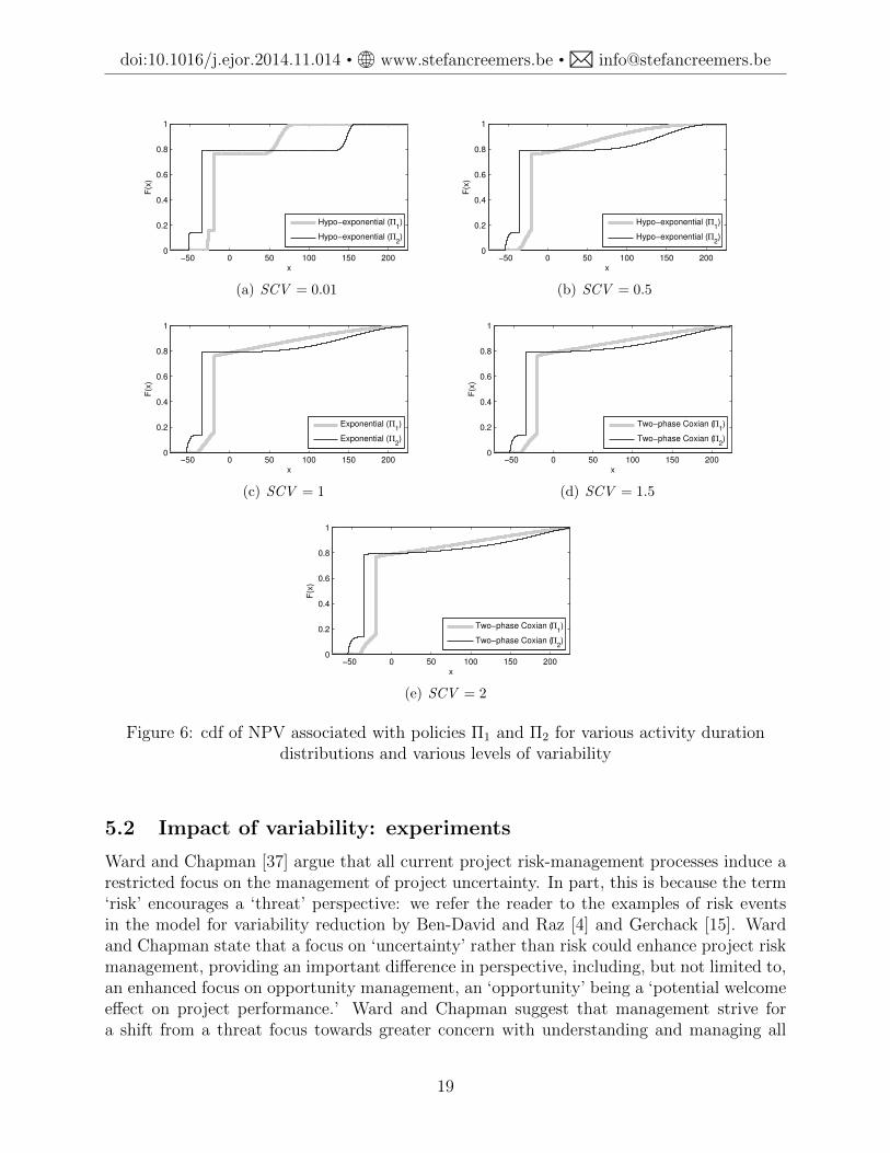
For policies Π1 and Π2 for the example instance, Figure 6 shows the NPV distribution(cdf) for a number of different values for SCV ; these plots were obtained via simulation.From module 1, policy Π1 only executes activity 1 while Π2 only executes activity 2, which islonger but less expensive, and has a slightly higher success probability. We observe that Π2

has both a higher upside potential (higher probability of achieving high NPV) as well as ahigher downside risk (larger chance of low NPV realizations); the net effect of this comparisonis favorable towards policy Π1 when SCV goes beyond the value of 0.2 (approximately).Apparently, the higher success probability and lower cost of activity 1 become more attractive(compared to activity 2) when the duration variability is higher, such that also low durationrealizations forD1 can be achieved, while higher-than-average realizations inD1 will probablynot affect the eNPV with the same magnitude because of the concave and non-increasingdependence of the discount factor with time. In other words, this example indicates that theinterplay between activity costs, success probabilities, average durations and the discountfactor induces the different dependence of Π1 and Π2 on SCV .

18





−50 0 50 100 150 2000

0.2

0.4

0.6

0.8

1

x

F(x

)

Hypo−exponential (Π1)


(a) SCV = 0.01

−50 0 50 100 150 2000

0.2

0.4

0.6

0.8

1

x

F(x

)



(b) SCV = 0.5

−50 0 50 100 150 2000

0.2

0.4

0.6

0.8

1

x

F(x

)

Exponential (Π1)

Exponential (Π2)

(c) SCV = 1

−50 0 50 100 150 2000

0.2

0.4

0.6

0.8

1

xF

(x)

Two−phase Coxian (Π1)


(d) SCV = 1.5

−50 0 50 100 150 2000

0.2

0.4

0.6

0.8

1

x

F(x

)



(e) SCV = 2

Figure 6: cdf of NPV associated with policies Π1 and Π2 for various activity durationdistributions and various levels of variability

5.2 Impact of variability: experiments

Ward and Chapman [37] argue that all current project risk-management processes induce arestricted focus on the management of project uncertainty. In part, this is because the term‘risk’ encourages a ‘threat’ perspective: we refer the reader to the examples of risk eventsin the model for variability reduction by Ben-David and Raz [4] and Gerchack [15]. Wardand Chapman state that a focus on ‘uncertainty’ rather than risk could enhance project riskmanagement, providing an important difference in perspective, including, but not limited to,an enhanced focus on opportunity management, an ‘opportunity’ being a ‘potential welcomeeffect on project performance.’ Ward and Chapman suggest that management strive fora shift from a threat focus towards greater concern with understanding and managing all

19





sources of uncertainty, with both up-side and down-side consequences, and explore andunderstand the origins of uncertainty before seeking to manage it. They suggest using theterm ‘uncertainty management,’ encompassing both ‘risk management’ and ‘opportunitymanagement.’ See also Loch et al. [25] for examples of how downside risks can sometimesbe turned into upside opportunity (e.g., p. 5 and p. 20).

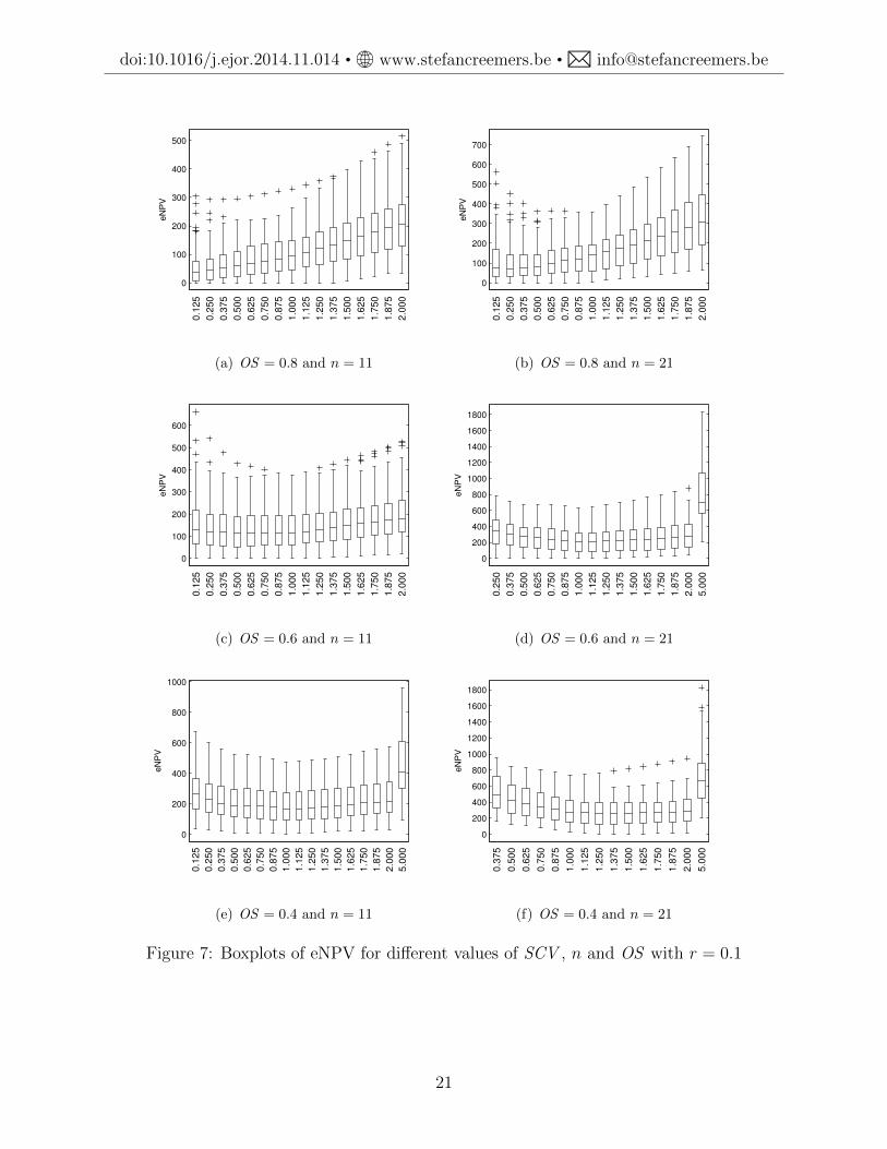
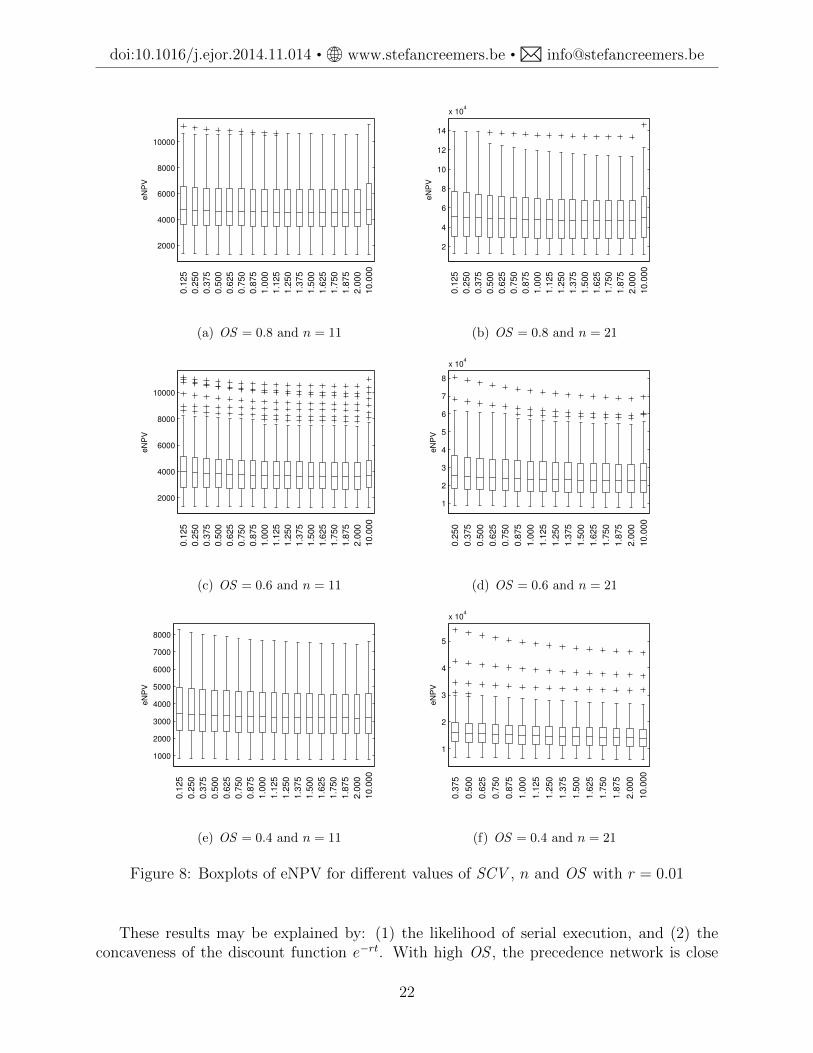
In order to examine the impact of duration variability on the value of a project in amore structured fashion, we have generated new instances in line with [9], with n ∈ {11, 21}and OS ∈ {0.4, 0.6, 0.8} but now we generate 100 instances per combination of parametersettings, and there is no activity failure nor modular completion of the project (each activityconstitutes a separate module). The payoff value C is (uniform) randomly chosen frominterval [0.9C0; 2C0], where C0 is the payoff value that associates objective value 0 (break-even) with the early-start policy ΠES for SCV = 1. We consider a wide range of SCV values;for more details on the generation of the duration distributions, see [11]. The results aregraphically summarized in Figure 7 for r = 10% and in Figure 8 for r = 1%. We investigatethe effect of different variability levels (different values of SCV ) on the value of the project.We observe that variability reduction is systematically not beneficial for the project’s valueas measured by eNPV in the cases where the precedence network is rather dense and thediscount rate is high; this corresponds with Figures 7(a), 7(b) and 7(c).

20





0

100

200

300

400

500

0.1

25

0.2

50

0.3

75

0.5

00

0.6

25

0.7

50

0.8

75

1.0

00

1.1

25

1.2

50

1.3

75

1.5

00

1.6

25

1.7

50

1.8

75

2.0

00

eN

PV

(a) OS = 0.8 and n = 11

0

100

200

300

400

500

600

700

0.1

25

0.2

50

0.3

75

0.5

00

0.6

25

0.7

50

0.8

75

1.0

00

1.1

25

1.2

50

1.3

75

1.5

00

1.6

25

1.7

50

1.8

75

2.0

00

eN

PV

(b) OS = 0.8 and n = 21

0

100

200

300

400

500

600

0.1

25

0.2

50

0.3

75

0.5

00

0.6

25

0.7

50

0.8

75

1.0

00

1.1

25

1.2

50

1.3

75

1.5

00

1.6

25

1.7

50

1.8

75

2.0

00

eN

PV

(c) OS = 0.6 and n = 11

0

200

400

600

800

1000

1200

1400

1600

1800

0.2

50

0.3

75

0.5

00

0.6

25

0.7

50

0.8

75

1.0

00

1.1

25

1.2

50

1.3

75

1.5

00

1.6

25

1.7

50

1.8

75

2.0

00

5.0

00

eN

PV

(d) OS = 0.6 and n = 21

0

200

400

600

800

1000

0.1

25

0.2

50

0.3

75

0.5

00

0.6

25

0.7

50

0.8

75

1.0

00

1.1

25

1.2

50

1.3

75

1.5

00

1.6

25

1.7

50

1.8

75

2.0

00

5.0

00

eN

PV

(e) OS = 0.4 and n = 11

0

200

400

600

800

1000

1200

1400

1600

1800

0.3

75

0.5

00

0.6

25

0.7

50

0.8

75

1.0

00

1.1

25

1.2

50

1.3

75

1.5

00

1.6

25

1.7

50

1.8

75

2.0

00

5.0

00

eN

PV

(f) OS = 0.4 and n = 21

Figure 7: Boxplots of eNPV for different values of SCV , n and OS with r = 0.1

21





2000

4000

6000

8000

10000

0.1

25

0.2

50

0.3

75

0.5

00

0.6

25

0.7

50

0.8

75

1.0

00

1.1

25

1.2

50

1.3

75

1.5

00

1.6

25

1.7

50

1.8

75

2.0

00

10.0

00

eN

PV

(a) OS = 0.8 and n = 11

2

4

6

8

10

12

14

x 104

0.1

25

0.2

50

0.3

75

0.5

00

0.6

25

0.7

50

0.8

75

1.0

00

1.1

25

1.2

50

1.3

75

1.5

00

1.6

25

1.7

50

1.8

75

2.0

00

10.0

00

eN

PV

(b) OS = 0.8 and n = 21

2000

4000

6000

8000

10000

0.1

25

0.2

50

0.3

75

0.5

00

0.6

25

0.7

50

0.8

75

1.0

00

1.1

25

1.2

50

1.3

75

1.5

00

1.6

25

1.7

50

1.8

75

2.0

00

10.0

00

eN

PV

(c) OS = 0.6 and n = 11

1

2

3

4

5

6

7

8

x 104

0.2

50

0.3

75

0.5

00

0.6

25

0.7

50

0.8

75

1.0

00

1.1

25

1.2

50

1.3

75

1.5

00

1.6

25

1.7

50

1.8

75

2.0

00

10.0

00

eN

PV

(d) OS = 0.6 and n = 21

1000

2000

3000

4000

5000

6000

7000

8000

0.1

25

0.2

50

0.3

75

0.5

00

0.6

25

0.7

50

0.8

75

1.0

00

1.1

25

1.2

50

1.3

75

1.5

00

1.6

25

1.7

50

1.8

75

2.0

00

10.0

00

eN

PV

(e) OS = 0.4 and n = 11

1

2

3

4

5

x 104

0.3

75

0.5

00

0.6

25

0.7

50

0.8

75

1.0

00

1.1

25

1.2

50

1.3

75

1.5

00

1.6

25

1.7

50

1.8

75

2.0

00

10.0

00

eN

PV

(f) OS = 0.4 and n = 21

Figure 8: Boxplots of eNPV for different values of SCV , n and OS with r = 0.01

These results may be explained by: (1) the likelihood of serial execution, and (2) theconcaveness of the discount function e−rt. With high OS , the precedence network is close

22





to serial, and an increase in duration variability results in an increase in the probabilityof completing the activity after a short amount of time. Due to the concave shape of thediscount function, the gain in the objective associated with low duration realizations canoffset the loss associated with higher duration realizations, and this is more pronounced forhigher r. Low OS , by contrast, will imply that activities are more often executed in parallel,and then the start of new activities is more frequently defined by the maximum of multipleactivity durations, the so-called merge (bias) effect [22]. This merge effect is less likelyto give rise to short completion times even in the event that some activity durations arelow, and thus reduces the benefits associated with the concave discount function. Optimalscheduling policies will indeed tend to execute some of the activities in parallel rather thanserially when possible (low OS ), because this reduces the project makespan and thus leadsto earlier project payoff.

Thus, investing in variability reduction becomes more interesting if: (1) r is low, (2) OSis low, and (3) variability can almost be eliminated. With a higher number n of activities,ceteris paribus, the project duration will also typically also be higher and there will be morechances for merge bias, so we would expect variability reduction to be more beneficial; this isalso confirmed by the experimental results. The figures also show that very high variabilityoften exhibits increased eNPV, but this phenomenon only occurs for unrealistically highSCV values (SCV = 10) in some of the settings. Similar patterns arise when activityfailures are included and when there may be more than one activity in the same module(which is not the case in the datasets to which the plots pertain). The effects are also notdependent on the PH-type character of the distributions: we have found comparable behaviorin simulations with lognormal and gamma distributions. As a final remark, we underlinethat all the observations made in this section pertain exclusively to expected NPV; obviously,lower duration variability is likely to induce lower variability in the NPV realizations as well,which may or may not be of significant importance to management, depending for instanceon whether an entire portfolio of projects or rather only one individual project is beingmanaged.

6 Policy class: experiments

Following up on the discussion in Section 3.1, we further examine the possible choices for thepolicy class. Table 5 contains the results for an experiment with which we evaluate whetherthe consideration of policies that start activities only at the end of other activities, is veryrestrictive. The experiments were run on the datasets with n = 11 and 21 that were usedin Section 5.2. We consider SCV ∈ {0.125, 0.25, 0.375, 0.5, 0.625, 0.75, 0.875, 1}. For n = 21and OS = 0.4, we do not report results for networks with SCV ∈ {0.125, 0.25}, and we alsodo not cover the combination n = 21, OS = 0.6 and SCV = 0.125. The reason for excludingsome combinations is that lower SCV requires more phases to model the activity durations:SCV = 0.25, for instance, requires four phases for each activity, which results in a networkof 4n phases. With r = 0.1 and for each value of SCV and OS , Table 5 reports the decreasein the objective value by optimizing over the restricted policy class as compared to the moregeneral class that also considers starting new activities after the completion of each phase ofeach ongoing activity; the decrease is expressed as a proportion of the payoff C and averaged

23





over the 100 instances.We conclude that the benefits of allowing activity start also at other times than only at

the completion of other activities are minor, and nowhere higher than around 0.3% of thepayoff. The benefits are higher especially when variability is low; this is logical, since thereare more phases and hence more decision times with lower SCV . The observation is alsoin line with the fact that for deterministic durations, late-start scheduling is optimal (seeSection 3.1). When SCV = 1, the two classes coincide. At the same time, there were nosignificant differences in the computational effort for finding an optimal member in the largerpolicy class. In other words, from a computational viewpoint, there is no real downside toallowing decisions to be made during the execution of activities, but the benefits are alsoquite limited. Other values of r have also been tested, with similar findings.

Table 5: Comparison of policy classes: average difference in eNPV as a proportion of thepayoff

SCV0.125 0.25 0.375 0.5 0.625 0.75 0.875 1

OS = 0.8 0.001 0.001 0.001 0.000 0.000 0.000 0.000 0.000n = 11 OS = 0.6 0.001 0.001 0.001 0.001 0.001 0.001 0.000 0.000

OS = 0.4 0.003 0.002 0.002 0.001 0.002 0.001 0.001 0.000OS = 0.8 0.000 0.000 0.000 0.000 0.000 0.000 0.000 0.000

n = 21 OS = 0.6 — 0.000 0.000 0.000 0.000 0.000 0.000 0.000OS = 0.4 — — 0.000 0.000 0.000 0.000 0.000 0.000

7 Summary and conclusions

Project planning with traditional tools typically ignores technological and duration uncer-tainty. In this article, we have explained how to model scheduling decisions in a morepractical environment with considerable uncertainty, and we illustrate how decision makingbased only on expected values can lead to inappropriate decisions. We have developed ageneric model for the optimal scheduling of R&D-project activities with stochastic dura-tions, non-zero failure probabilities and multiple trials subject to precedence constraints.We assess the effect of different degrees of activity duration variability on the expected NPVof a project. We also refute the intuition that an increase in uncertainty necessarily entailsa decrease of system performance, which seconds the proposal to focus also on ‘opportunitymanagement’ rather than only on ‘risk management’: we illustrate that higher operationalvariability does not always lead to lower project values, meaning that (sometimes costly)variance reduction strategies are not always advisable.

References

[1] W. J. Abernathy and R. S. Rosenbloom, “Parallel strategies in development projects,”Management Science, vol. 15, no. 10, pp. 486–505, 1969.

24





[2] V. G. Adlakha and V. G. Kulkarni, “A classified bibliography of research on stochasticPERT networks,” INFOR, vol. 27, no. 3, pp. 272–296, 1989.

[3] C. Y. Baldwin and K. B. Clark, Design Rules: The Power of Modularity. Cambridge,MA, USA: The MIT Press, 2000.

[4] I. Ben-David and T. Raz, “An integrated approach for risk response development inproject planning,” Journal of the Operational Research Society, vol. 52, no. 1, pp. 14–25,2001.

[5] S. Benati, “An optimization model for stochastic project networks with cash flows,”Computational Management Science, vol. 3, no. 4, pp. 271–284, 2006.

[6] A. H. Buss and M. J. Rosenblatt, “Activity delay in stochastic project networks,” Oper-ations Research, vol. 45, no. 1, pp. 126–139, 1997.

[7] S. Chopra and P. Meindl, Supply Chain Management: Strategy, Planning, and Operation,New Jersey, USA: Prentice Hall, 2013.

[8] Y. H. Chun, “Sequential decisions under uncertainty in the R&D project selection prob-lem,” IEEE Transactions on Engineering Management, vol. 41, no. 4, pp. 404–413, 1994.

[9] K. Coolen, W. Wei, F. Talla Nobibon, and R. Leus, “Scheduling modular projects on abottleneck resource,” Journal of Scheduling, vol. 17, no. 1, pp. 67–85, 2014.

[10] S. Creemers, R. Leus, and M. Lambrecht, “Scheduling Markovian PERT networks tomaximize the net present value,” Operations Research Letters, vol. 38, no. 1, pp. 51–56,2010.

[11] S. Creemers, B. De Reyck, and R. Leus, “Project planning with alternative technologiesin uncertain environments,” KU Leuven, Faculty of Business and Economics, Departmentof Decision Sciences and Information Management working paper #1314, 2013.

[12] B. De Reyck and R. Leus, “R&D-project scheduling when activities may fail,” IIETransactions, vol. 40, no. 4, pp. 367–384, 2008.

[13] M. Ding and J. Eliashberg, “Structuring the new product development pipeline,” Man-agement Science, vol. 48, no. 3, pp. 343–363, 2002.

[14] S. Elmaghraby, Activity Networks: Project Planning and Control by Network Models,New York, NY, USA: John Wiley & Sons Inc, 1977.

[15] Y. Gerchak, “On the allocation of uncertainty-reduction effort to minimize total vari-ability,” IIE Transactions, vol. 32, no. 5, pp. 403–407, 2000.

[16] J. Gittins and J. Y. Yu, “Software for managing the risks and improving the profitabil-ity of pharmaceutical research,” International Journal of Technology Intelligence andPlanning, vol. 3, no. 4, pp. 305–316, 2007.

25





[17] D. Granot and D. Zuckerman, “Optimal sequencing and resource allocation in researchand development projects,” Management Science, vol. 37, no. 2, pp. 140–156, 1991.

[18] J. N. Hagstrom, “Computational complexity of PERT problems,” Networks, vol. 18, pp.139–147, 1988.

[19] M. Huysmans, K. Coolen, F. Talla Nobibon and R. Leus, “A fast greedy heuristic forscheduling modular projects,” KU Leuven, Faculty of Business and Economics, Depart-ment of Decision Sciences and Information Management working paper #1227, 2012.

[20] G. Igelmund and F. J. Radermacher, “Preselective strategies for the optimization ofstochastic project networks under resource constraints,” Networks, vol. 13, no. 1, pp.1–28, 1983.

[21] V. Jain and I. E. Grossmann, “Resource-constrained scheduling of tests in new productdevelopment,” Industrial & Engineering Chemistry Research, vol. 38, no. 8, pp. 3013–3026, 1999.

[22] A.R.Jr. Klingel, “Bias in Pert project completion time calculations for a real network,”Management Science, vol. 13, no. 4, pp. B-194–B-101, 1966.

[23] V. Kulkarni and V. Adlakha, “Markov and Markov-regenerative PERT networks,” Op-erations Research, vol. 34, no. 5, pp. 769–781, 1986.

[24] L. Lenfle, “The strategy of parallel approaches in projects with unforeseeable uncer-tainty: The Manhattan case in retrospect,” International Journal of Project Manage-ment, vol. 29, no. 4, pp. 359–373, 2011.

[25] C. H. Loch, A. DeMeyer, and M. T. Pich, Managing the Unknown: A New Approach toManaging High Uncertainty and Risk in Projects, Hoboken, NJ, USA: Wiley, 2006.

[26] A. Ludwig, R. M. Mohring, and F. Stork, “A computational study on bounding themakespan distribution in stochastic project networks,” Annals of Operations Research,vol. 102, pp. 49–64, 2001.

[27] R. H. Mohring, “Scheduling under uncertainty: Optimizing against a randomizing ad-versary,” Lecture Notes in Computer Science, vol. 1913, pp. 15–26, 2000.

[28] R. H. Mohring, “Scheduling under uncertainty: Bounding the makespan distribution,”Lecture Notes in Computer Science, vol. 2122, pp. 79–97, 2001.

[29] R. R. Nelson, “Uncertainty, learning, and the economics of parallel research and devel-opment efforts,” The Review of Economics and Statistics, vol. 43, no. 4, pp. 351–364,1961.

[30] M. F. Neuts, Matrix-Geometric Solutions in Stochastic Models, Baltimore, MD, USA:Johns Hopkins University Press, 1981.

[31] W. B. Powell, “What you should know about Approximate Dynamic Programming,”Naval Research Logistics, vol. 56, pp. 239–249, 2009.

26





[32] M. Puterman, Markov Decision Processes: Discrete Stochastic Dynamic Programming,John Wiley & Sons Inc, 1994.

[33] C. W. Schmidt and I. E. Grossmann, “Optimization models for the scheduling of testingtasks in new product development,” Industrial & Engineering Chemistry Research, vol.35, no. 10, pp. 3498–3510, 1996.

[34] M. J. Sobel, J. G. Szmerekovsky, and V. Tilson, “Scheduling projects with stochasticactivity duration to maximize expected net present value,” European Journal of Opera-tional Research, vol. 198, no. 1, pp. 697–705, 2009.

[35] S. C. Sommer and C. H. Loch, “Selectionism and learning in projects with complexityand unforeseeable uncertainty,” Management Science, vol. 50, no. 10, pp. 1334–1347,2004.

[36] F. Stork, “Stochastic resource-constrained project scheduling,” Technische UniversitatBerlin, PhD Thesis, 2001.

[37] S. Ward and C. Chapman, “Transforming project risk management into project uncer-tainty management,” International Journal of Project Management, vol. 21, pp. 97–105,2003.

[38] M. L. Weitzman, “Optimal search for the best alternative,” Econometrica, vol. 47, no.3, pp. 641–654, 1979.

[39] J. Y. Yu and J. Gittins, “Models and software for improving the profitability of phar-maceutical research,” European Journal of Operational Research, vol. 189, no. 2, pp.459–475, 2008.

27




Documents

Project planning with alternative technologies in