Project Number: WMC 2228

COMSOL Assisted Modeling of a Climbing Film Evaporator

A Major Qualifying Project Report

Submitted to the Faculty

of the

WORCESTER POLYTECHNIC INSTITUTE

in partial fulfillment of the requirements for the

Degree of Bachelor of Science

by

_______________________________________

Miguel A Herrera

Date: April 30, 2010

Approved:

_________________________________________

Professor William M. Clark, Project Advisor

i

Abstract The aim of this project was to create a computer model of a climbing film evaporator using COMSOL Multiphysics. We used the designed climbing film evaporator lab for CHE 4402 to structure our lab experiment and to collect lab data about the change of composition in the evaporator feed solution. The data was then used to create a simulation model using COMSOL Multiphysics. COMSOL approximated the experimental data very well predicting a product concentration of 12.8 percent glycerol in water whereas in the experiment the measured concentration was 12 percent. The energy balance results did not match very closely with COMSOL reporting 5758 W of heat given by the steam whereas in the experiment the calculated heat given by the steam was 7384 W. We concluded that COMSOL can be an effective way for simulating a climbing film evaporator given the correct heat transfer coefficients, heat flux expressions, boundary conditions, and concentrations and we developed recommendations, which we present regarding future modeling and experimentation.

ii

Acknowledgements

The success of our project depended on the contributions of two individuals over the past four months. We would like to take time to thank all of those who have helped and supported us in this process.

First, we want to thank our advisor, Professor William M. Clark for his guidance throughout the project. His supervision during the laboratory experiment and his inputs on the development of the COMSOL model were invaluable.

Next, we would like to thank Mr. Jack Ferraro for setting the experiment for us and always being available for assistance.

iii

Contents Abstract .......................................................................................................................................................... i

Acknowledgements ....................................................................................................................................... ii

Introduction .................................................................................................................................................. 1

Background and Theory ................................................................................................................................ 2

Methodology ................................................................................................................................................. 7

Part 1: Conducting the experiment on the Climbing Film Evaporator ..................................................... 7

Theory behind the calculations ............................................................................................................... 10

Part 2: Modeling the process on COMSOL ............................................................................................. 16

Results and Discussion ................................................................................................................................ 30

Part 1: Results for the Mass Balance on the Climbing Film Evaporator ................................................. 30

Part 2: Results for the Energy Balance on the Climbing Film Evaporator ............................................... 33

Part 3: Overall Heat Transfer Coefficient results .................................................................................... 35

Part 4: Results for Evaporator Economy and Capacity ........................................................................... 39

Part 5: COMSOL Modeling Results .......................................................................................................... 41

Conclusions ................................................................................................................................................. 44

Recommendations ...................................................................................................................................... 45

References .................................................................................................................................................. 46

Appendix A- Sample Calculations ........................................................................................................... 47

Appendix B- COMSOL Model Report ...................................................................................................... 57

Appendix C- Extra Graphs and Tables ..................................................................................................... 70

Appendix D- Raw Data and Spreadsheet containing calculations .......................................................... 71

iv

Table of Figures

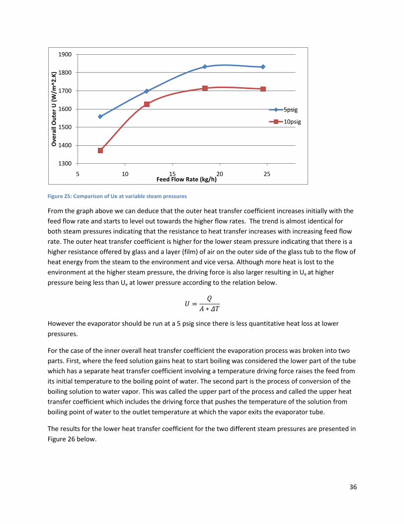
Figure 1: Example of concentrating a liquid by using evaporation as a unit operation. .............................. 2 Figure 2: Image of a climbing film evaporator. ............................................................................................. 3 Figure 3: Schematic showing the flow of liquid and vapor in the CFE .......................................................... 4 Figure 4: Different modules available in COMSO ......................................................................................... 6 Figure 5: Schematic of the Climbing Film Evaporator ................................................................................... 7 Figure 6: Block diagram of the evaporator (Mass Balance) ........................................................................ 10 Figure 7: Block diagram of the CFE for energy balance calculations ......................................................... 12 Figure 8: Model Navigator Screen .............................................................................................................. 17 Figure 9: Draw Object Screen ..................................................................................................................... 18 Figure 10: Geometry ................................................................................................................................... 19 Figure 11: COMSOL Constants .................................................................................................................... 20 Figure 12: COMSOL Global Expressions ...................................................................................................... 21 Figure 13: chcd Subdomain Settings ........................................................................................................... 22 Figure 14: chcc Subdomain Settings ........................................................................................................... 23 Figure 15: chcc2 Subdomain Settings ......................................................................................................... 24 Figure 16: chcd Boundary Conditions ......................................................................................................... 25 Figure 17: chcc Boundary Conditions ......................................................................................................... 26 Figure 18: chcc2 Boundary Conditions ....................................................................................................... 27 Figure 19: Extrusion Coupling Values.......................................................................................................... 28 Figure 20: Experimental results comparing glycerol concentration at different steam pressures ............ 31 Figure 21: Comparison of experimental and theoretical glycerol in the product @10 psig ...................... 32 Figure 22: Trend followed by QP at variable steam pressures ................................................................... 33 Figure 23: Trend followed by QE for variable steam pressure and feed flow rate ..................................... 34 Figure 24: Comparison of QP and QE with varying flow rates at 5 psig ..................................................... 35 Figure 25: Comparison of Ue at variable steam pressures ......................................................................... 36 Figure 26: Comparison of the Ulower at different steam pressures .......................................................... 37 Figure 27: Comparison of the U(upper) at different steam pressures ....................................................... 38 Figure 28: Comparison of U lower and U upper at 10 psig ......................................................................... 38 Figure 29: Evaporator Economy at variable steam pressures .................................................................... 39 Figure 30: Evaporator Economy at variable steam pressures .................................................................... 40 Figure 31: Concentration of glycerol throughout the length of the climbing film evaporator .................. 41 Figure 32: Glycerol in water concentration profile ..................................................................................... 42 Figure 33: Temperature profile ................................................................................................................... 43 Figure 34: Percentage glycerol v/s feed flow rate at 5 psig ........................................................................ 70 Figure 35: Comparison of QP and QE with varying flow rate at 10 psig ..................................................... 71 Figure 36: Comparison of Ulower at different steam pressures ................................................................ 71

v

Table of Tables Table 1: Calculated values for input and output flow rates @ 5 psig ......................................................... 30 Table 2: Calculated values for input and output flow rates @ 10 psig ....................................................... 30 Table 3: Calculated values for percentage glycerol in the condenser solution .......................................... 30 Table 4: Calculated values for heat gained by the process and heat lost to the environment. ................. 33 Table 5: Experimental and COMSOL results Qs and Ws ............................................................................. 42 Table 6: Experimental and COMSOL Heat Transfer Coefficients ................................................................ 43

1

Introduction With the development of technology powerful simulation softwares have become more readily

available to the public. Computer simulation makes it easier for people to better understand complicated physical phenomena that occur in apparatuses used to design certain chemical engineering processes. This is possible because these simulations are able to provide visual representation of otherwise hard to picture concepts such as, concentration gradients, velocity profiles and temperature gradients. Although running these processes first hand in the laboratory is an excellent way to complement theoretical knowledge and understand the basic principles and theories behind these unit operations it can be very useful to have digital simulations that virtually model these processes and provide illustrations of basic chemical engineering principles virtually. One such software is COMSOL Multiphysics. COMSOL is a finite element analysis and solver software package for coupled phenomena or Multiphysics. It is particularly good at modeling chemical engineering apparatus since it is specifically designed to easily combine transport phenomena, computational fluid dynamics and mass and energy transport to chemical reaction kinetics. COMSOL has the ability to solve multiple non linear PDE’s simultaneously and the models can be generated and solved in one, two or even three dimensions [13]. COMSOL Multiphysics is a very helpful tool as the models are very interactive and user friendly and ideal tools to complement theoretical knowledge in classrooms, lab tutorials and study guides.

The objective of this project was to create a COMSOL model for a climbing film evaporator. In brief, a climbing film evaporator is a unit operation in which a solution is concentrated by removing a part of the solvent in the form of vapor [3]. The most commonly used solvent is water and the latent heat of evaporation is usually supplied by condensing steam. Heat from the steam is transmitted to the solution by conduction and convection through the glass wall of the evaporator. When the solvent starts boiling the bubbles inside the tube create an upward flow that causes the mixture to rise [6] and finally sloshes over to a container were the concentrated solution is collected. Similarly, the vaporized solvent is collected in a separate container after going through a condenser. Climbing film evaporators are widely used in the food and drink industry as means to concentrate fruit juices, coffee and tea. They are also used to recover expensive solvents from solutions that otherwise would be wasted.

In order to create the model, first we performed an experiment using the climbing film evaporator located in the Unit Operations Laboratory following the designed experiment guidelines for course CHE 4402. In short, for the experiment we had a solution of 10 percent glycerol in water that was fed to the evaporator. Several runs were performed using different feed flow rates and steam pressures. We recorded the concentration of the product as well as the flow rate, the flow rate of the condensate, and the flow rate of the condenser solution. We performed mass balances and energy balances on the system to calculate heat transfer coefficients, heat lost to the environment and heat given by the steam. The results obtained from the experimental calculations were then used to create a COMSOL model of our climbing film evaporator. This project explains and illustrates the climbing film evaporation process and strives to model the same behavior using COMSOL Multiphysics to aid future users in understanding the process.

2

Background and Theory

Background for Climbing Film Evaporator

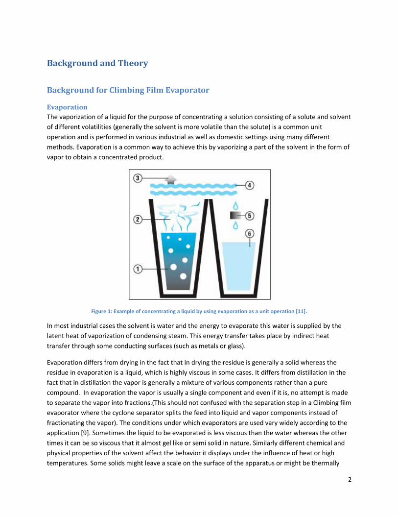
Evaporation The vaporization of a liquid for the purpose of concentrating a solution consisting of a solute and solvent of different volatilities (generally the solvent is more volatile than the solute) is a common unit operation and is performed in various industrial as well as domestic settings using many different methods. Evaporation is a common way to achieve this by vaporizing a part of the solvent in the form of vapor to obtain a concentrated product.

Figure 1: Example of concentrating a liquid by using evaporation as a unit operation [11].

In most industrial cases the solvent is water and the energy to evaporate this water is supplied by the latent heat of vaporization of condensing steam. This energy transfer takes place by indirect heat transfer through some conducting surfaces (such as metals or glass).

Evaporation differs from drying in the fact that in drying the residue is generally a solid whereas the residue in evaporation is a liquid, which is highly viscous in some cases. It differs from distillation in the fact that in distillation the vapor is generally a mixture of various components rather than a pure compound. In evaporation the vapor is usually a single component and even if it is, no attempt is made to separate the vapor into fractions.(This should not confused with the separation step in a Climbing film evaporator where the cyclone separator splits the feed into liquid and vapor components instead of fractionating the vapor). The conditions under which evaporators are used vary widely according to the application [9]. Sometimes the liquid to be evaporated is less viscous than the water whereas the other times it can be so viscous that it almost gel like or semi solid in nature. Similarly different chemical and physical properties of the solvent affect the behavior it displays under the influence of heat or high temperatures. Some solids might leave a scale on the surface of the apparatus or might be thermally

3

unstable or damageable under the influence of heat energy. These variations in the chemical compound behaviors and the applications of the process (industrial or domestic) have led to various types of designs for evaporators.

Evaporator types can be classified as [2]:

• Jacketed Vessels

• Coils

• Horizontal tube evaporators

• Short tube vertical evaporators

• Long tube vertical evaporators o Forced circulation o Upward flow (climbing film) o Downward flow (falling film)

• Forced Circulation Evaporators

• Flash Evaporators

Climbing Film Evaporator A climbing film evaporator is a type of long tube vertical evaporator. A CFE is a shell and tube heat exchanger mounted to a vapor/liquid separator [6].

Figure 2: Image of a climbing film evaporator [6].

These evaporators are generally operated under vacuum in order to reduce the boiling point of the feed solution and increase the heat flux. The principle behind the CFE is that any kind of vapor (steam in our case) flowing at a higher velocity than the liquid (glycerol solution in our case) flows into the cavity

4

between the two glass tubes of the evaporator causing the liquid to rise up the inner tube in a film[6]. The feed solution enters the bottom of the inner tube and flows upwards as a result of forced circulation due to a pump. In the lower section of the tube the feed solution is heated up to the boiling point of the solvent. At some height in the inner tube bubbles start to form indicating that the more volatile substance has attained its boiling point. This height is called the boiling height of the liquid. The ascending force of the water vapor produced during boiling causes the liquid and the vapor to rise upwards in parallel flow. At the same time the production of water vapor increases and the product starts to form a thin film on the walls of the inner tube of the evaporator and the liquid mixture begins to rise upwards. This co-current flow of the liquid and the vapor against gravity creates a high degree of turbulence in the liquid. This results higher linear velocity and rate of heat transfer and is beneficial during evaporation of highly viscous products or products that have a tendency to foul the surface of the evaporator [8]. In this boiling zone a mixture of vapor and liquid tend to rise quickly to the top of the tube and are discharged at high velocity from the top. They are sent into the cyclone separator which then separates them to be sent to the product line or condenser.

Figure 3: Schematic showing the flow of liquid and vapor in the CFE [10]

A lot of times this type of evaporator is used with product recirculation, where some of the concentrated product is recycled back into the feed solution (just like in cases of distillation) in order to concentrate the product further and produce sufficient liquid loading inside the heating tubes.

Advantages of using the climbing film evaporator include [6]:

• Reduced floor space requirements

• Higher heat transfer coefficient due to partial two-phase flow

• Ability to handle foamy liquids

5

• Low residence time which permits the use of CFE’s for heat sensitive materials such as food products or thermally unstable chemicals.

• Another advantage of using the climbing film evaporator is the low cost of construction.

The disadvantages include:

• Higher pressure drop through the tube compared to other tubular evaporators

• High head- room requirements

Multitube CFE’s are often used in the industry to concentrate solutions such as fruit juices that can be damaged by prolonged heat. Some of the most common uses of the CFE include concentration of cane

sugar syrups, black liquor in paper plants, nitrates and electrolytic tinning liquors [2].

Each climbing film evaporator is set with certain major and minor equipment which are as follows [2]:

• A condenser

• Vacuum producing pump

• Condensate removing steam traps

• Process Pumps

• Process Piping

• Safety and Relief Equipment such as valves

• Thermal Insulation

• Process Vessels

• Electronic monitors and flow meters

Background for COMSOL There are various unit operations which are used to design certain chemical engineering process whether they are in the industry or small scale laboratories. Although running these processes first hand in the laboratory is an excellent way to complement theoretical knowledge and understand the basic principles and theories behind these unit operations it can be very useful to have digital simulations that virtually model these processes and provide illustrations of basic chemical engineering principles.

One such programming package used to simulate various chemical engineering processes is COMSOL Multiphysics. This is a finite element analysis and solver software package for coupled phenomena or Multiphysics [13]. There is a special chemical engineering module which is a great tool for process related modeling. It is specifically designed to easily combine transport phenomena, computational fluid dynamics and mass and energy transport to chemical reaction kinetics. COMSOL has the ability to solve multiple non linear PDE’s simultaneously and the models can be generated and solved in one, two or even three dimensions [13]. COMSOL Multiphysics is a very helpful tool as the models are very interactive and user friendly and ideal tools to complement theoretical knowledge in classrooms, lab tutorials and study guides.

6

Figure 4: Different modules available in COMSOL [13]

The following are the basic steps to create a model in COMSOL:

Generate the geometry of the process that you want to simulate. This geometry can also be imported from other sources. Different geometries can be selected based on the dimensions of the process model. The geometry then requires to be meshed in order to create a grid of small, simple shaped data points that the program can solve. The size and type of mesh depend on the desired final process. After creating a meshed geometry the physics of the process being solved can be defined in the sub domain settings and then known values and constants can be entered to solve the model. Once the program has solved the model the post processing of the results enables the user to generate variation profiles, maps and plots of process variables. These can be extrapolated or interpolated in time or beyond parametric solutions.

7

Methodology

Part 1: Conducting the Experiment on the Climbing Film Evaporator

Schematic of the Climbing Film Evaporator

Figure 5: Schematic of the Climbing Film Evaporator [12]

Equipment Summary The climbing film evaporator is a tower consisting of two concentric glass tubes. The dimensions of the CFE in Goddard Hall 116 were measured and the inner diameter was found to be 1 inch, the outer diameter was 2.5 inches and the length of the glass tubes was measured to be 9 ft. The evaporator is connected to a pump and rotameter which supply the feed solution to be concentrated into the inner tube of the evaporator valves control the flow of liquids through these pipes into the glass tube. There is a line which supplies steam to the cavity between the inner and outer tubes and valves and a pressure gauge control the flow of this steam. As part of the feed vaporizes it exits the tube and enters a cyclone separator which separates the vapor and sends it to the condenser and sends the liquid to the product tank to be collected. The product line is also equipped with valves to control the flow and collection of liquid. The vapor that enters the condenser is condensed and sent to the condensate tank to be collected. The steam that exits the outer tube goes into a steam trap where it condenses and this condensate is constantly drained to avoid buildup.

8

Operating the climbing film evaporator The main objective of this experiment was to determine the effect of varying the feed flow rate and steam pressure on the performance of the evaporator which is evaluated by heat transfer coefficients and the concentration of glycerol in the product solution.

The climbing film evaporator present in Goddard Hall 116 was used to conduct this experiment in two trials. During the first run the operating steam pressure was maintained constant at a certain value and the feed flow rates were varied. During the second trial the steam pressure was varied and same feed flow rates, as trial 1, were used again. Since the maximum steam pressure available in the Goddard Hall evaporator is 25 psig, operating pressure was always maintained below this value.

Procedure 1. Opened the valves connected to the steam supply line to drain any water that might have

condensed and could possibly skew our data. Once the water had been drained the valve was closed.

2. Recorded the values of room temperature, steam temperature and atmospheric pressure. 3. Took a sample out of the feed tank and used the density meter provided to measure the specific

gravity and hence the percentage glycerol of the feed solution. (This step was carried out just to verify t he composition of the feed solution which is indicated to be 10%).

4. Weighed the steam condensate collection bucket, the product solution bucket and the condenser solution bucket and placed them under their respective tanks.

5. Opened the valve on the cooling water line for the condenser to start the supply of cooling water to the process.

6. Opened the valve on the steam supply line to start pumping steam into the evaporator’s outer glass tube. Selected a pressure of steam (5psig) and let it be constant for the rest of the experiment.

7. Turned on the pump and set a volumetric flow rate value (120 ml/min in the digital flow meter). Once the process had started we could observe steam going into the glass evaporator tube and the feed solution being pumped into the inner tube.

8. To ensure that the evaporator actually works smoothly and ensure that the process attains steady state a couple of runs were made without taking any data and analysis of the product and condenser solutions collected. We let the process run for around ten minutes to ensure that operating steam pressure, feed flow rate etc were constant throughout the runs.

9. After ensuring the process runs smoothly we started collecting data. Waited for a while to let the system attain steady state. (This time is variable for each flow rate and steam pressure but can be approximated to a minimum of 20 minutes for each run).

10. Started draining the product solution by opening the valve at the base of the product collection line. After completely draining the product reservoir, the valve was closed again for a period of two minutes and product was allowed to collect in the product tank. This interval was timed using a stop watch and the end of two minutes the valve was opened again to drain the collected product into an empty bucket that had already been weighed.

11. Weighed this product to determine the mass flow rate of the product.

9

12. Drained the condenser solution by opening the valve at the base of the condenser line. After draining the valve was closed again and an interval of two minutes was timed to collect condenser solution over. At the end of two minutes the valve was opened and water collected in the condenser reservoir was drained into a pre-weighed empty bucket.

13. Weighed this condenser solution to determine the condenser mass flow rate. 14. Collected the steam condensate over a period of two minutes and weighed it to determine the

steam flow rate into the process. 15. Took a sample from the hot product solution into a beaker and immersed it into an ice bath to

be cooled to ambient (room temperature). 16. Measured the specific gravity of this cooled sample using the density meter and determined the

corresponding percentage of glycerol in the product from the water- glycerol solution specific gravity chart provided.

17. Repeated the above process for three other feed flow rates (200 ml/min, 300 ml/min and 400 ml/min) keeping everything else constant.

Day 2

1. Repeated the entire process above at a constant steam pressure of 10 psig and four different flow rates of (120, 200, 300 and 400 ml/min).

Shutdown Procedure

To ensure the safe shut down of the apparatus make sure the following steps are taken:

• Close the feed supply line by closing the valve it is equipped with.

• Close the steam control valve and all the other steam valves.

• Stop the feed pump.

• Open all valves at the bottom of product and condenser lines to drain any excess liquid.

• Leave the cooling water running even after the process has been shut down

Safety Precautions In order to maintain a safe working environment in the laboratory the following safety precautions were taken:

• Check that all the valves are working properly and no air or water inlets/ outlets are blocked.

• Ensure that the pump and the flow meter are functioning correctly.

• Ensure that the steam trap is functioning correctly in order to avoid any steam or hot condensate being trapped.

• The maximum steam pressure that can be supplied to the evaporator is 25 psig. Ensure that the operating steam pressure never exceeds this value.

• Since this is a very energy intensive experiment a lot of heat is lost to the environment through the apparatus. Consequently a lot of the equipment gets extremely hot. Ensure that gloves are worn at all times when touching such equipment and to avoid contact with hot surfaces as much as possible.

10

• The steam condensate and the product solution both exit the apparatus at extremely high temperatures. Wear thick gloves whenever collecting these two liquids. Be very careful during the collection since the hot liquid or steam can splash and cause burns and injuries.

• Leave the cooling water flow on even after closing the steam line and feed supply line. Cooling water cools down the apparatus after the experiment is over to ensure that there is no overheating of equipment causing potential damage or safety concerns.

• Wear hard hats and goggles and appropriate lab safety equipment at all times in the lab.

Theory behind the calculations

Mass Balance Calculations One of the major objectives of this experiment was to understand how the feed flow rate affects the final concentration of the product solution. In order to estimate the affect of varying feed flow rate on the other variables and parameters of the climbing film evaporator mass balance was calculated on the evaporator and the relevant theory and procedures are outlined below.

The structure of the climbing film evaporator can be basically broken down into a simple block diagram showing the major streams going in and out of the evaporator. The basic diagram for the evaporator looks as follows:

In order to calculate the mass balance we need the mass flow rates of all the inlet and outlet streams. Since we recorded the feed flow rate using a flow meter it is a volumetric flow rate with units (ml/min) and need to be converted to mass flow rate. Since the solution is a mixture of water and glycerol its

Figure 6: Block diagram of the evaporator (Mass Balance)

11

density would be a combination of the densities of water and glycerol. The equation below was used to perform this conversion.

�𝜌𝜌𝑓𝑓𝑓𝑓𝑓𝑓𝑓𝑓 � = (𝜌𝜌𝐺𝐺𝐺𝐺𝐺𝐺 ∗ 𝑥𝑥𝑓𝑓𝑔𝑔𝐺𝐺𝐺𝐺 ) + (𝜌𝜌𝑤𝑤 ∗ 𝑥𝑥𝑓𝑓𝑤𝑤 ) (1)

Where:

𝜌𝜌𝑓𝑓𝑓𝑓𝑓𝑓𝑓𝑓 = 𝐴𝐴𝐴𝐴𝑓𝑓𝐴𝐴𝐴𝐴𝑔𝑔𝑓𝑓 𝑓𝑓𝑓𝑓𝑑𝑑𝑑𝑑𝑑𝑑𝑑𝑑𝐺𝐺 𝑜𝑜𝑓𝑓 𝑑𝑑ℎ𝑓𝑓 𝑓𝑓𝑓𝑓𝑓𝑓𝑓𝑓 𝑑𝑑𝑜𝑜𝐺𝐺𝑠𝑠𝑑𝑑𝑑𝑑𝑜𝑜𝑑𝑑 �𝑔𝑔𝑐𝑐𝑐𝑐3�

𝜌𝜌𝐺𝐺𝐺𝐺𝐺𝐺 = 𝐷𝐷𝑓𝑓𝑑𝑑𝑑𝑑𝑑𝑑𝑑𝑑𝐺𝐺 𝑜𝑜𝑓𝑓 𝑔𝑔𝐺𝐺𝐺𝐺𝑐𝑐𝑓𝑓𝐴𝐴𝑜𝑜𝐺𝐺 �𝑔𝑔𝑐𝑐𝑐𝑐3�

𝑥𝑥𝑓𝑓𝑔𝑔𝐺𝐺𝐺𝐺 = 𝑊𝑊𝑓𝑓𝑑𝑑𝑔𝑔ℎ𝑑𝑑 𝑓𝑓𝐴𝐴𝐴𝐴𝑐𝑐𝑑𝑑𝑜𝑜𝑑𝑑 𝑜𝑜𝑓𝑓 𝑔𝑔𝐺𝐺𝐺𝐺𝑐𝑐𝑓𝑓𝐴𝐴𝑜𝑜𝐺𝐺 𝑑𝑑𝑑𝑑 𝑑𝑑ℎ𝑓𝑓 𝑑𝑑𝑜𝑜𝐺𝐺𝑠𝑠𝑑𝑑𝑑𝑑𝑜𝑜𝑑𝑑

𝜌𝜌𝑤𝑤 = 𝐷𝐷𝑓𝑓𝑑𝑑𝑑𝑑𝑑𝑑𝑑𝑑𝐺𝐺 𝑜𝑜𝑓𝑓 𝑤𝑤𝐴𝐴𝑑𝑑𝑓𝑓𝐴𝐴 �𝑔𝑔𝑐𝑐𝑐𝑐3�

𝑥𝑥𝑓𝑓𝑤𝑤 = 𝑊𝑊𝑓𝑓𝑑𝑑𝑔𝑔ℎ𝑑𝑑 𝑓𝑓𝐴𝐴𝐴𝐴𝑐𝑐𝑑𝑑𝑜𝑜𝑑𝑑 𝑜𝑜𝑓𝑓 𝑔𝑔𝐺𝐺𝐺𝐺𝑐𝑐𝑓𝑓𝐴𝐴𝑜𝑜𝐺𝐺 𝑑𝑑𝑑𝑑 𝑑𝑑ℎ𝑓𝑓 𝑑𝑑𝑜𝑜𝐺𝐺𝑠𝑠𝑑𝑑𝑑𝑑𝑜𝑜𝑑𝑑 The next step was to convert the volumetric flow rate into mass flow rate as shown in Equation 2 below.

�̇�𝑐𝑓𝑓 = �̇�𝑉 ∗ 𝜌𝜌𝑓𝑓𝑓𝑓𝑓𝑓𝑓𝑓 (2)

Where:

�̇�𝑐𝑓𝑓 = 𝑀𝑀𝐴𝐴𝑑𝑑𝑑𝑑 𝐹𝐹𝐺𝐺𝑜𝑜𝑤𝑤 𝑅𝑅𝐴𝐴𝑑𝑑𝑓𝑓 𝑜𝑜𝑓𝑓 𝑑𝑑ℎ𝑓𝑓 𝐹𝐹𝑓𝑓𝑓𝑓𝑓𝑓 �𝑘𝑘𝑔𝑔ℎ �

�̇�𝑉 = 𝑉𝑉𝑜𝑜𝐺𝐺𝑠𝑠𝑐𝑐𝑓𝑓𝑑𝑑𝐴𝐴𝑑𝑑𝑐𝑐 𝐹𝐹𝐺𝐺𝑜𝑜𝑤𝑤 𝑅𝑅𝐴𝐴𝑑𝑑𝑓𝑓 𝑜𝑜𝑓𝑓 𝑑𝑑ℎ𝑓𝑓 𝐹𝐹𝑓𝑓𝑓𝑓𝑓𝑓 (𝑐𝑐𝐺𝐺𝑐𝑐𝑑𝑑𝑑𝑑

)

For the purpose of calculating mass balance we are going to assume that the condenser solution flow rate that we measured was accurate and use those values to calculate the mass balance. We assumed that the product flow rate we measured was not quite accurate owing to the fact that we collected it only over a period of 2 minutes and the fact that the sloshing over of the liquid might have been very erratic and not uniform (it might have sloshed over a lot of solution consecutively and the next minute there might have been very low amount of liquid. We have to take an average of these to find the correct flow rate and for that we should have collected the product over a longer period of time (maybe around 4-5 minutes).

Keeping this in mind we calculated the product flow rate with Equation [1] given below.

�̇�𝑐𝑃𝑃 = �̇�𝑐𝑓𝑓 − �̇�𝑐𝐴𝐴 (3)

Where:

�̇�𝑐𝑃𝑃 = 𝑀𝑀𝐴𝐴𝑑𝑑𝑑𝑑 𝐹𝐹𝐺𝐺𝑜𝑜𝑤𝑤 𝑅𝑅𝐴𝐴𝑑𝑑𝑓𝑓 𝑜𝑜𝑓𝑓 𝑑𝑑ℎ𝑓𝑓 𝑝𝑝𝐴𝐴𝑜𝑜𝑓𝑓𝑠𝑠𝑐𝑐𝑑𝑑 �𝑘𝑘𝑔𝑔ℎ�

�̇�𝑐𝐴𝐴 = 𝑀𝑀𝐴𝐴𝑑𝑑𝑑𝑑 𝐹𝐹𝐺𝐺𝑜𝑜𝑤𝑤 𝑅𝑅𝐴𝐴𝑑𝑑𝑓𝑓 𝑜𝑜𝑓𝑓 𝑑𝑑ℎ𝑓𝑓 𝑐𝑐𝑜𝑜𝑑𝑑𝑓𝑓𝑓𝑓𝑑𝑑𝑑𝑑𝑓𝑓𝐴𝐴 𝑑𝑑𝑜𝑜𝐺𝐺𝑠𝑠𝑑𝑑𝑑𝑑𝑜𝑜𝑑𝑑 �𝑘𝑘𝑔𝑔ℎ�

Using similar balances as Equation 3 above us calculated the concentration of glycerol and water in the condenser and product solutions [1].

�̇�𝑐𝑝𝑝𝑔𝑔𝐺𝐺𝐺𝐺 = �̇�𝑐𝑓𝑓𝑔𝑔𝐺𝐺𝐺𝐺 − �̇�𝑐𝐴𝐴𝑔𝑔𝐺𝐺𝐺𝐺 (4)

Where:

12

�̇�𝑐𝑝𝑝𝑔𝑔𝐺𝐺𝐺𝐺 = 𝑀𝑀𝐴𝐴𝑑𝑑𝑑𝑑 𝐹𝐹𝐺𝐺𝑜𝑜𝑤𝑤 𝑅𝑅𝐴𝐴𝑑𝑑𝑓𝑓 𝑜𝑜𝑓𝑓 𝑑𝑑ℎ𝑓𝑓 𝑔𝑔𝐺𝐺𝐺𝐺𝑐𝑐𝑓𝑓𝐴𝐴𝑜𝑜𝐺𝐺 𝑑𝑑𝑑𝑑 𝑑𝑑ℎ𝑓𝑓 𝑝𝑝𝐴𝐴𝑜𝑜𝑓𝑓𝑠𝑠𝑐𝑐𝑑𝑑 �𝑘𝑘𝑔𝑔ℎ�

�̇�𝑐𝑓𝑓𝑔𝑔𝐺𝐺𝐺𝐺 = 𝑀𝑀𝐴𝐴𝑑𝑑𝑑𝑑 𝐹𝐹𝐺𝐺𝑜𝑜𝑤𝑤 𝑅𝑅𝐴𝐴𝑑𝑑𝑓𝑓 𝑜𝑜𝑓𝑓 𝑑𝑑ℎ𝑓𝑓 𝑔𝑔𝐺𝐺𝐺𝐺𝑐𝑐𝑓𝑓𝐴𝐴𝑜𝑜𝐺𝐺 𝑑𝑑𝑑𝑑 𝑑𝑑ℎ𝑓𝑓 𝑓𝑓𝑓𝑓𝑓𝑓𝑓𝑓 �𝑘𝑘𝑔𝑔ℎ�

�̇�𝑐𝐴𝐴𝑔𝑔𝐺𝐺𝐺𝐺 = 𝑀𝑀𝐴𝐴𝑑𝑑𝑑𝑑 𝐹𝐹𝐺𝐺𝑜𝑜𝑤𝑤 𝑅𝑅𝐴𝐴𝑑𝑑𝑓𝑓 𝑜𝑜𝑓𝑓 𝑑𝑑ℎ𝑓𝑓 𝑔𝑔𝐺𝐺𝐺𝐺𝑐𝑐𝑓𝑓𝐴𝐴𝑜𝑜𝐺𝐺 𝑑𝑑𝑑𝑑 𝑑𝑑ℎ𝑓𝑓 𝐴𝐴𝐴𝐴𝑝𝑝𝑜𝑜𝐴𝐴 �𝑘𝑘𝑔𝑔ℎ�

And similarly calculated the mass balance on water within the process [1]

�̇�𝑐𝑝𝑝𝑊𝑊 = �̇�𝑐𝑓𝑓𝑊𝑊 − �̇�𝑐𝐴𝐴𝑊𝑊 (5)

Where:

�̇�𝑐𝑝𝑝𝑊𝑊 = 𝑀𝑀𝐴𝐴𝑑𝑑𝑑𝑑 𝐹𝐹𝐺𝐺𝑜𝑜𝑤𝑤 𝑅𝑅𝐴𝐴𝑑𝑑𝑓𝑓 𝑜𝑜𝑓𝑓 𝑑𝑑ℎ𝑓𝑓 𝑤𝑤𝐴𝐴𝑑𝑑𝑓𝑓𝐴𝐴 𝑑𝑑𝑑𝑑 𝑑𝑑ℎ𝑓𝑓 𝑝𝑝𝐴𝐴𝑜𝑜𝑓𝑓𝑠𝑠𝑐𝑐𝑑𝑑 𝑑𝑑𝑑𝑑𝐴𝐴𝑓𝑓𝐴𝐴𝑐𝑐 �𝑘𝑘𝑔𝑔ℎ�

�̇�𝑐𝑓𝑓𝑊𝑊 = 𝑀𝑀𝐴𝐴𝑑𝑑𝑑𝑑 𝐹𝐹𝐺𝐺𝑜𝑜𝑤𝑤 𝑅𝑅𝐴𝐴𝑑𝑑𝑓𝑓 𝑜𝑜𝑓𝑓 𝑑𝑑ℎ𝑓𝑓 𝑔𝑔𝐺𝐺𝐺𝐺𝑐𝑐𝑓𝑓𝐴𝐴𝑜𝑜𝐺𝐺 𝑑𝑑𝑑𝑑 𝑑𝑑ℎ𝑓𝑓 𝑓𝑓𝑓𝑓𝑓𝑓𝑓𝑓 𝑑𝑑𝑑𝑑𝐴𝐴𝑓𝑓𝐴𝐴𝑐𝑐 �𝑘𝑘𝑔𝑔ℎ�

�̇�𝑐𝐴𝐴𝑊𝑊 = 𝑀𝑀𝐴𝐴𝑑𝑑𝑑𝑑 𝐹𝐹𝐺𝐺𝑜𝑜𝑤𝑤 𝑅𝑅𝐴𝐴𝑑𝑑𝑓𝑓 𝑜𝑜𝑓𝑓 𝑑𝑑ℎ𝑓𝑓 𝑔𝑔𝐺𝐺𝐺𝐺𝑐𝑐𝑓𝑓𝐴𝐴𝑜𝑜𝐺𝐺 𝑑𝑑𝑑𝑑 𝑑𝑑ℎ𝑓𝑓 𝐴𝐴𝐴𝐴𝑝𝑝𝑜𝑜𝐴𝐴 𝑑𝑑𝑑𝑑𝐴𝐴𝑓𝑓𝐴𝐴𝑐𝑐 �𝑘𝑘𝑔𝑔ℎ�

The next step was to calculate the theoretical percentage of glycerol (as predicted by theory) in the product solution to compare it to the experimental results obtained.

�̇�𝑐𝑓𝑓 ∗ 𝑥𝑥𝑓𝑓𝑔𝑔𝐺𝐺𝐺𝐺 = �̇�𝑐𝑝𝑝 ∗ 𝑥𝑥𝑝𝑝𝑔𝑔𝐺𝐺𝐺𝐺 (6)

Energy Balance Calculations The next step is to calculate the energy balance to see how much energy is utilized by the evaporator to vaporize water and concentrate glycerol and how much of the energy supplied is lost to the environment. This will not only help us to calculate the energy loss but also help us evaluate the economy and efficiency of the climbing film evaporator. This information will help us weigh the performance of the evaporator against the energy losses and help us decide whether the process is economically feasible or not.

Figure 7: Block diagram of the CFE for energy balance calculations

13

The heat lost by the steam is given by the following relations [1]:

𝑄𝑄𝑆𝑆 = �̇�𝑐𝑑𝑑𝜆𝜆𝑑𝑑 (7)

Where:

�̇�𝑐𝑑𝑑 = Condensate mass flow rate (𝑘𝑘𝑔𝑔𝑑𝑑𝑓𝑓𝑐𝑐

)

𝜆𝜆𝑑𝑑 = 𝐿𝐿𝐴𝐴𝑑𝑑𝑓𝑓𝑑𝑑𝑑𝑑 𝐻𝐻𝑓𝑓𝐴𝐴𝑑𝑑 𝑜𝑜𝑓𝑓 𝐴𝐴𝐴𝐴𝑝𝑝𝑜𝑜𝐴𝐴𝑑𝑑𝑣𝑣𝐴𝐴𝑑𝑑𝑑𝑑𝑜𝑜𝑑𝑑 𝑜𝑜𝑓𝑓 𝑑𝑑ℎ𝑓𝑓 𝑑𝑑𝑑𝑑𝑓𝑓𝐴𝐴𝑐𝑐 �𝑘𝑘𝑘𝑘𝑘𝑘𝑔𝑔�

𝑄𝑄𝑆𝑆 = 𝑄𝑄𝑝𝑝 + 𝑄𝑄𝐸𝐸 (8)

𝑄𝑄𝑆𝑆 = �̇�𝑐𝐴𝐴𝜆𝜆 + �̇�𝑐𝑓𝑓𝐶𝐶𝑝𝑝𝑓𝑓𝛥𝛥𝛥𝛥 + 𝑄𝑄𝐸𝐸 (9)

Where: 𝑄𝑄𝐸𝐸 = 𝐸𝐸𝑑𝑑𝑓𝑓𝐴𝐴𝑔𝑔𝐺𝐺 𝐺𝐺𝑜𝑜𝑑𝑑𝑑𝑑𝑓𝑓𝑑𝑑 𝑑𝑑𝑜𝑜 𝑑𝑑ℎ𝑓𝑓 𝑓𝑓𝑑𝑑𝐴𝐴𝑑𝑑𝐴𝐴𝑜𝑜𝑑𝑑𝑐𝑐𝑓𝑓𝑑𝑑𝑑𝑑 (W)

𝜆𝜆 = 𝐿𝐿𝐴𝐴𝑑𝑑𝑓𝑓𝑑𝑑𝑑𝑑 𝐻𝐻𝑓𝑓𝐴𝐴𝑑𝑑 𝐶𝐶𝐴𝐴𝑝𝑝𝐴𝐴𝑐𝑐𝑑𝑑𝑑𝑑𝐺𝐺 𝑜𝑜𝑓𝑓 𝑑𝑑ℎ𝑓𝑓 𝑑𝑑𝑜𝑜𝐺𝐺𝑠𝑠𝑑𝑑𝑑𝑑𝑜𝑜𝑑𝑑 �𝑘𝑘𝑘𝑘𝑘𝑘𝑔𝑔�

𝐶𝐶𝑝𝑝𝑓𝑓 = 𝐴𝐴𝐴𝐴𝑓𝑓𝐴𝐴𝐴𝐴𝑔𝑔𝑓𝑓 𝑆𝑆𝑝𝑝𝑓𝑓𝑐𝑐𝑑𝑑𝑓𝑓𝑑𝑑𝑐𝑐 𝐻𝐻𝑓𝑓𝐴𝐴𝑑𝑑 𝐶𝐶𝐴𝐴𝑝𝑝𝐴𝐴𝑐𝑐𝑑𝑑𝑑𝑑𝐺𝐺 𝑜𝑜𝑓𝑓 𝑑𝑑ℎ𝑓𝑓 𝑓𝑓𝑓𝑓𝑓𝑓𝑓𝑓 𝑑𝑑𝑜𝑜𝐺𝐺𝑠𝑠𝑑𝑑𝑑𝑑𝑜𝑜𝑑𝑑 (𝑘𝑘

𝑘𝑘𝑔𝑔 ∗ 𝐾𝐾)

𝛥𝛥𝛥𝛥 = �𝛥𝛥𝑏𝑏𝑜𝑜𝑑𝑑𝐺𝐺𝑑𝑑𝑑𝑑𝑔𝑔 −𝛥𝛥𝑓𝑓𝑓𝑓𝑓𝑓𝑓𝑓 � (𝐾𝐾) In equation 8 given above the latent heat of vaporization (𝜆𝜆) is not the latent heat of condenser solution as we would expect it to be but is rather the latent heat for the feed solution. This latent heat is not constant and varies as the concentration of glycerol (any solute) in water varies. The values of this hence not taken to be 2769 kJ/kg but rather found out to be 1600 kJ/kg as given by Pacheco and Frioni [4]. (The heat gained by the process was then calculated using the Equation 10 [1] below:

𝑄𝑄𝑝𝑝 = [�̇�𝑐𝑓𝑓𝐶𝐶𝑝𝑝𝑓𝑓 ∗ �𝛥𝛥𝑏𝑏 − 𝛥𝛥𝑓𝑓�] + [�̇�𝑐𝐴𝐴𝜆𝜆𝑓𝑓] (10)

Where: 𝑄𝑄𝑝𝑝 = 𝐸𝐸𝑑𝑑𝑓𝑓𝐴𝐴𝑔𝑔𝐺𝐺 𝑔𝑔𝐴𝐴𝑑𝑑𝑑𝑑𝑓𝑓𝑓𝑓 𝑏𝑏𝐺𝐺 𝑑𝑑ℎ𝑓𝑓 𝑝𝑝𝐴𝐴𝑜𝑜𝑐𝑐𝑓𝑓𝑑𝑑𝑑𝑑 (𝑊𝑊)

𝜆𝜆𝑓𝑓 = 𝐿𝐿𝐴𝐴𝑑𝑑𝑓𝑓𝑑𝑑𝑑𝑑 𝐻𝐻𝑓𝑓𝐴𝐴𝑑𝑑 𝐶𝐶𝐴𝐴𝑝𝑝𝐴𝐴𝑐𝑐𝑑𝑑𝑑𝑑𝐺𝐺 𝑜𝑜𝑓𝑓 𝑑𝑑ℎ𝑓𝑓 𝑓𝑓𝑓𝑓𝑓𝑓𝑓𝑓 𝑑𝑑𝑜𝑜𝐺𝐺𝑠𝑠𝑑𝑑𝑑𝑑𝑜𝑜𝑑𝑑 �𝑘𝑘𝑘𝑘𝑘𝑘𝑔𝑔�

The heat lost to the environment was calculated using the overall energy balance for the evaporator given in Equation 11[1].

𝑄𝑄𝑆𝑆 = 𝑄𝑄𝑝𝑝 + 𝑄𝑄𝐸𝐸 (11)

𝑄𝑄𝐸𝐸 = 𝑄𝑄𝑆𝑆 − 𝑄𝑄𝑝𝑝

14

Heat Transfer Coefficient Calculations

Calculating the outer heat transfer coefficient In the climbing film evaporator energy is constantly being exchanged between the steam and the process through convection and phase change between glass and the atmosphere and the glass and the feed solution. The overall heat transfer coefficient is the ability of a series of resistive materials or boundaries to transfer heat [1].

The overall heat transfer coefficient takes into account the individual heat transfer coefficients of each stream and the resistance of the pipe material. It can be calculated as the reciprocal of the sum of a series of thermal resistances such as:

𝑄𝑄𝑆𝑆 = 𝑄𝑄𝑝𝑝 + 𝑄𝑄𝐸𝐸 (11)

1𝑈𝑈𝐴𝐴

=1

ℎ𝑑𝑑 ∗ 𝐴𝐴𝑑𝑑+

𝑞𝑞𝑘𝑘𝑞𝑞 ∗ 𝐴𝐴

+1

ℎ𝑜𝑜 ∗ 𝐴𝐴𝑜𝑜 (12)

For the process of concentrating glycerol using the climbing film evaporator there is an outer overall heat transfer coefficient which is given by the expression [1]:

𝑄𝑄𝐸𝐸 = 𝑈𝑈𝑂𝑂𝐸𝐸 ∗ 𝐴𝐴𝑂𝑂 ∗ ∆𝛥𝛥𝐿𝐿𝑀𝑀 (13)

Where: 𝑈𝑈𝑂𝑂𝐸𝐸 = 𝑂𝑂𝑠𝑠𝑑𝑑𝑓𝑓𝐴𝐴 ℎ𝑓𝑓𝐴𝐴𝑑𝑑 𝑑𝑑𝐴𝐴𝐴𝐴𝑑𝑑𝑑𝑑𝑓𝑓𝑓𝑓𝐴𝐴 𝑐𝑐𝑜𝑜𝑓𝑓𝑓𝑓𝑓𝑓𝑑𝑑𝑐𝑐𝑑𝑑𝑓𝑓𝑑𝑑𝑑𝑑 (𝑊𝑊/(𝑐𝑐2.𝐾𝐾) 𝐴𝐴𝑂𝑂 = 𝑂𝑂𝑠𝑠𝑑𝑑𝑓𝑓𝐴𝐴 𝑑𝑑𝑠𝑠𝐴𝐴𝑓𝑓𝐴𝐴𝑐𝑐𝑓𝑓 𝐴𝐴𝐴𝐴𝑓𝑓𝐴𝐴 𝑜𝑜𝑓𝑓 𝑑𝑑ℎ𝑓𝑓 𝑓𝑓𝐴𝐴𝐴𝐴𝑝𝑝𝑜𝑜𝐴𝐴𝐴𝐴𝑑𝑑𝑜𝑜𝐴𝐴 (𝑐𝑐2) ∆𝛥𝛥𝐿𝐿𝑀𝑀 = 𝑑𝑑𝑑𝑑 𝑑𝑑ℎ𝑓𝑓 𝐿𝐿𝑜𝑜𝑔𝑔 𝑐𝑐𝑓𝑓𝐴𝐴𝑑𝑑 𝑑𝑑𝑓𝑓𝑐𝑐𝑝𝑝𝑓𝑓𝐴𝐴𝐴𝐴𝑑𝑑𝑠𝑠𝐴𝐴𝑓𝑓 𝑓𝑓𝑑𝑑𝑓𝑓𝑓𝑓𝑓𝑓𝐴𝐴𝑓𝑓𝑑𝑑𝑐𝑐𝑓𝑓 ( 𝑤𝑤ℎ𝑑𝑑𝑐𝑐ℎ 𝑑𝑑𝑑𝑑 𝑑𝑑ℎ𝑑𝑑𝑑𝑑 𝑐𝑐𝐴𝐴𝑑𝑑𝑓𝑓 𝑑𝑑𝑑𝑑 𝑗𝑗𝑠𝑠𝑑𝑑𝑑𝑑 (𝛥𝛥𝑑𝑑 − 𝛥𝛥𝐴𝐴))

Using the already calculated values the energy lost to the environment from Equation 11 we can rearrange Equation 13 [1]:

𝑈𝑈𝑂𝑂𝐸𝐸 =𝑄𝑄𝐸𝐸

𝐴𝐴𝑂𝑂 ∗ (𝛥𝛥𝑑𝑑 − 𝛥𝛥𝐴𝐴) (14)

Calculating the inner heat transfer coefficient In case of the evaporator process the inner heat transfer can be calculated in two ways:

• Consider the entire tube as a whole and neglect the phase change happening in the tube and consider the driving force to be between the feed inlet temperature and the outlet temperature

• Break down the tube into two processes o One where the feed gets heated and the height of the evaporator is taken to be the

height at which the glycerol solution starts boiling. The heat transfer coefficient using these conditions is called the lower overall heat transfer coefficient.

15

o And the rest of the process where the water starts to evaporate (the height is considered to be the total height minus the boiling height) is used to calculate the upper heat transfer coefficient.

𝑄𝑄𝑃𝑃 = 𝑈𝑈𝐺𝐺 ∗ 𝐴𝐴𝐺𝐺 ∗ ∆𝛥𝛥𝐿𝐿𝑀𝑀 + 𝑈𝑈𝑠𝑠 ∗ 𝐴𝐴𝑠𝑠 ∗ ∆𝛥𝛥𝐿𝐿𝑀𝑀 (15)

Where: 𝑈𝑈𝐺𝐺 = 𝐿𝐿𝑜𝑜𝑤𝑤𝑓𝑓𝐴𝐴 ℎ𝑓𝑓𝐴𝐴𝑑𝑑 𝑑𝑑𝐴𝐴𝐴𝐴𝑑𝑑𝑑𝑑𝑓𝑓𝑓𝑓𝐴𝐴 𝑐𝑐𝑜𝑜𝑓𝑓𝑓𝑓𝑓𝑓𝑑𝑑𝑐𝑐𝑑𝑑𝑓𝑓𝑑𝑑𝑑𝑑 𝑓𝑓𝑜𝑜𝐴𝐴 𝑑𝑑ℎ𝑓𝑓 𝑝𝑝𝐴𝐴𝑜𝑜𝑐𝑐𝑓𝑓𝑑𝑑𝑑𝑑 (𝑊𝑊/(𝑐𝑐2.𝐾𝐾) 𝐴𝐴𝐺𝐺 = 𝐴𝐴𝐴𝐴𝑓𝑓𝐴𝐴 𝑜𝑜𝑓𝑓 𝑑𝑑ℎ𝑓𝑓 𝐺𝐺𝑜𝑜𝑤𝑤𝑓𝑓𝐴𝐴 𝑝𝑝𝐴𝐴𝐴𝐴𝑑𝑑 𝑜𝑜𝑓𝑓 𝑑𝑑ℎ𝑓𝑓 𝑑𝑑𝑠𝑠𝑏𝑏𝑓𝑓 (𝑐𝑐2) ∆𝛥𝛥𝐿𝐿𝑀𝑀 = 𝑑𝑑𝑑𝑑 𝑑𝑑ℎ𝑓𝑓 𝐿𝐿𝑜𝑜𝑔𝑔 𝑐𝑐𝑓𝑓𝐴𝐴𝑑𝑑 𝑑𝑑𝑓𝑓𝑐𝑐𝑝𝑝𝑓𝑓𝐴𝐴𝐴𝐴𝑑𝑑𝑠𝑠𝐴𝐴𝑓𝑓 𝑓𝑓𝑑𝑑𝑓𝑓𝑓𝑓𝑓𝑓𝐴𝐴𝑓𝑓𝑑𝑑𝑐𝑐𝑓𝑓 (𝐾𝐾) 𝑈𝑈𝑠𝑠 = 𝑈𝑈𝑝𝑝𝑝𝑝𝑓𝑓𝐴𝐴 ℎ𝑓𝑓𝐴𝐴𝑑𝑑 𝑑𝑑𝐴𝐴𝐴𝐴𝑑𝑑𝑑𝑑𝑓𝑓𝑓𝑓𝐴𝐴 𝑐𝑐𝑜𝑜𝑓𝑓𝑓𝑓𝑓𝑓𝑑𝑑𝑐𝑐𝑑𝑑𝑓𝑓𝑑𝑑𝑑𝑑 𝑓𝑓𝑜𝑜𝐴𝐴 𝑑𝑑ℎ𝑓𝑓 𝑝𝑝𝐴𝐴𝑜𝑜𝑐𝑐𝑓𝑓𝑑𝑑𝑑𝑑 (𝑊𝑊/(𝑐𝑐2.𝐾𝐾) 𝐴𝐴𝑠𝑠 = 𝐴𝐴𝐴𝐴𝑓𝑓𝐴𝐴 𝑜𝑜𝑓𝑓 𝑑𝑑ℎ𝑓𝑓 𝑠𝑠𝑝𝑝𝑝𝑝𝑓𝑓𝐴𝐴 𝑝𝑝𝐴𝐴𝐴𝐴𝑑𝑑 𝑜𝑜𝑓𝑓 𝑑𝑑ℎ𝑓𝑓 𝑑𝑑𝑠𝑠𝑏𝑏𝑓𝑓 (𝑐𝑐2)

We can break down the inner tube into lower and upper tubes and the heat gained by the process also gets divided in a similar manner. The heat gained by the process in the lower part of the tube is given by Equation 16 [1].

𝑄𝑄𝐺𝐺 = �̇�𝑐𝑓𝑓 ∗ 𝐶𝐶𝑝𝑝 ∗ �𝛥𝛥𝑏𝑏 − 𝛥𝛥𝑓𝑓� (16)

Where: 𝑄𝑄𝐺𝐺 = 𝐻𝐻𝑓𝑓𝐴𝐴𝑑𝑑 𝑔𝑔𝐴𝐴𝑑𝑑𝑑𝑑𝑓𝑓𝑓𝑓 𝑏𝑏𝐺𝐺 𝑑𝑑ℎ𝑓𝑓 𝑓𝑓𝑓𝑓𝑓𝑓𝑓𝑓 𝑑𝑑𝑑𝑑 𝑑𝑑ℎ𝑓𝑓 𝐺𝐺𝑜𝑜𝑤𝑤𝑓𝑓𝐴𝐴 𝑝𝑝𝐴𝐴𝐴𝐴𝑑𝑑 𝑜𝑜𝑓𝑓 𝑑𝑑ℎ𝑓𝑓 𝑑𝑑𝑠𝑠𝑏𝑏𝑓𝑓 (𝑊𝑊) Once the heat gained has been calculated we can now utilize this value to calculate the inner heat transfer coefficient in the lower part of the tube:

𝑄𝑄𝐺𝐺 = 𝑈𝑈𝐺𝐺 ∗ 𝐴𝐴𝐺𝐺 ∗ ∆𝛥𝛥𝐿𝐿𝑀𝑀 (17)

Where: 𝑈𝑈𝐺𝐺 = 𝐿𝐿𝑜𝑜𝑤𝑤𝑓𝑓𝐴𝐴 ℎ𝑓𝑓𝐴𝐴𝑑𝑑 𝑑𝑑𝐴𝐴𝐴𝐴𝑑𝑑𝑑𝑑𝑓𝑓𝑓𝑓𝐴𝐴 𝑐𝑐𝑜𝑜𝑓𝑓𝑓𝑓𝑓𝑓𝑑𝑑𝑐𝑐𝑑𝑑𝑓𝑓𝑑𝑑𝑑𝑑 𝑓𝑓𝑜𝑜𝐴𝐴 𝑑𝑑ℎ𝑓𝑓 𝑝𝑝𝐴𝐴𝑜𝑜𝑐𝑐𝑓𝑓𝑑𝑑𝑑𝑑 (𝑊𝑊/(𝑐𝑐2.𝐾𝐾) 𝐴𝐴𝐺𝐺 = 𝐴𝐴𝐴𝐴𝑓𝑓𝐴𝐴 𝑜𝑜𝑓𝑓 𝑑𝑑ℎ𝑓𝑓 𝐺𝐺𝑜𝑜𝑤𝑤𝑓𝑓𝐴𝐴 𝑝𝑝𝐴𝐴𝐴𝐴𝑑𝑑 𝑜𝑜𝑓𝑓 𝑑𝑑ℎ𝑓𝑓 𝑑𝑑𝑠𝑠𝑏𝑏𝑓𝑓 (𝑐𝑐2) ∆𝛥𝛥𝐿𝐿𝑀𝑀[1] = 𝑑𝑑𝑑𝑑 𝑑𝑑ℎ𝑓𝑓 𝐿𝐿𝑜𝑜𝑔𝑔 𝑐𝑐𝑓𝑓𝐴𝐴𝑑𝑑 𝑑𝑑𝑓𝑓𝑐𝑐𝑝𝑝𝑓𝑓𝐴𝐴𝐴𝐴𝑑𝑑𝑠𝑠𝐴𝐴𝑓𝑓 𝑓𝑓𝑑𝑑𝑓𝑓𝑓𝑓𝑓𝑓𝐴𝐴𝑓𝑓𝑑𝑑𝑐𝑐𝑓𝑓 (𝐾𝐾) which in this case is given by the equation below:

∆𝛥𝛥𝐿𝐿𝑀𝑀 =��𝛥𝛥𝑑𝑑 − 𝛥𝛥𝑓𝑓� − (𝛥𝛥𝑑𝑑 − 𝛥𝛥𝑏𝑏)�

ln��𝛥𝛥𝑑𝑑 − 𝛥𝛥𝑓𝑓�𝛥𝛥𝑑𝑑 − 𝛥𝛥𝑏𝑏

� (18)

Where: 𝛥𝛥𝑑𝑑 = 𝛥𝛥𝑓𝑓𝑐𝑐𝑝𝑝𝑓𝑓𝐴𝐴𝐴𝐴𝑑𝑑𝑠𝑠𝐴𝐴𝑓𝑓 𝑜𝑜𝑓𝑓 𝑑𝑑ℎ𝑓𝑓 𝑑𝑑𝑑𝑑𝑓𝑓𝐴𝐴𝑐𝑐 (𝐾𝐾) 𝛥𝛥𝑓𝑓 = 𝛥𝛥𝑓𝑓𝑐𝑐𝑝𝑝𝑓𝑓𝐴𝐴𝐴𝐴𝑑𝑑𝑠𝑠𝐴𝐴𝑓𝑓 𝑜𝑜𝑓𝑓 𝑑𝑑ℎ𝑓𝑓 𝑓𝑓𝑓𝑓𝑓𝑓𝑓𝑓 (𝐾𝐾) 𝛥𝛥𝑏𝑏 = 𝛥𝛥𝑓𝑓𝑐𝑐𝑝𝑝𝑓𝑓𝐴𝐴𝐴𝐴𝑑𝑑𝑠𝑠𝐴𝐴𝑓𝑓 𝐴𝐴𝑑𝑑 𝑤𝑤ℎ𝑑𝑑𝑐𝑐ℎ 𝑑𝑑ℎ𝑓𝑓 𝑓𝑓𝑓𝑓𝑓𝑓𝑓𝑓 𝑑𝑑𝑜𝑜𝐺𝐺𝑠𝑠𝑑𝑑𝑑𝑑𝑜𝑜𝑑𝑑 𝑑𝑑𝑑𝑑𝐴𝐴𝐴𝐴𝑑𝑑𝑑𝑑 𝑑𝑑𝑜𝑜 𝑏𝑏𝑜𝑜𝑑𝑑𝐺𝐺 (𝐾𝐾) The heat gained by the process in the upper part of the tube is given by Equation 19 [1].

16

𝑄𝑄𝑠𝑠 = �̇�𝑐𝐴𝐴 ∗ 𝜆𝜆 (19)

Where: 𝑄𝑄𝑠𝑠 = 𝐻𝐻𝑓𝑓𝐴𝐴𝑑𝑑 𝑔𝑔𝐴𝐴𝑑𝑑𝑑𝑑𝑓𝑓𝑓𝑓 𝑏𝑏𝐺𝐺 𝑑𝑑ℎ𝑓𝑓 𝑓𝑓𝑓𝑓𝑓𝑓𝑓𝑓 𝑑𝑑𝑑𝑑 𝑑𝑑ℎ𝑓𝑓 𝑠𝑠𝑝𝑝𝑝𝑝𝑓𝑓𝐴𝐴 𝑝𝑝𝐴𝐴𝐴𝐴𝑑𝑑 𝑜𝑜𝑓𝑓 𝑑𝑑ℎ𝑓𝑓 𝑑𝑑𝑠𝑠𝑏𝑏𝑓𝑓 (𝑊𝑊) 𝜆𝜆 𝑑𝑑 = 𝐿𝐿𝐴𝐴𝑑𝑑𝑓𝑓𝑑𝑑𝑑𝑑 ℎ𝑓𝑓𝐴𝐴𝑑𝑑 𝑜𝑜𝑓𝑓 𝐴𝐴𝐴𝐴𝑝𝑝𝑜𝑜𝐴𝐴𝑑𝑑𝑣𝑣𝐴𝐴𝑑𝑑𝑑𝑑𝑜𝑜𝑑𝑑 𝑜𝑜𝑓𝑓 𝑑𝑑𝑑𝑑𝑓𝑓𝐴𝐴𝑐𝑐 And once this energy has been calculated we can easily determine the upper heat transfer coefficient by the relation below [1]:

𝑄𝑄𝑠𝑠 = 𝑈𝑈𝑠𝑠 ∗ 𝐴𝐴𝑠𝑠 ∗ ∆𝛥𝛥𝐿𝐿𝑀𝑀 (20)

𝑈𝑈𝑠𝑠 = 𝑈𝑈𝑝𝑝𝑝𝑝𝑓𝑓𝐴𝐴 ℎ𝑓𝑓𝐴𝐴𝑑𝑑 𝑑𝑑𝐴𝐴𝐴𝐴𝑑𝑑𝑑𝑑𝑓𝑓𝑓𝑓𝐴𝐴 𝑐𝑐𝑜𝑜𝑓𝑓𝑓𝑓𝑓𝑓𝑑𝑑𝑐𝑐𝑑𝑑𝑓𝑓𝑑𝑑𝑑𝑑 𝑓𝑓𝑜𝑜𝐴𝐴 𝑑𝑑ℎ𝑓𝑓 𝑝𝑝𝐴𝐴𝑜𝑜𝑐𝑐𝑓𝑓𝑑𝑑𝑑𝑑 (𝑊𝑊/(𝑐𝑐2.𝐾𝐾) 𝐴𝐴𝑠𝑠 = 𝐴𝐴𝐴𝐴𝑓𝑓𝐴𝐴 𝑜𝑜𝑓𝑓 𝑑𝑑ℎ𝑓𝑓 𝑠𝑠𝑝𝑝𝑝𝑝𝑓𝑓𝐴𝐴 𝑝𝑝𝐴𝐴𝐴𝐴𝑑𝑑 𝑜𝑜𝑓𝑓 𝑑𝑑ℎ𝑓𝑓 𝑑𝑑𝑠𝑠𝑏𝑏𝑓𝑓 (𝑐𝑐2) ∆𝛥𝛥𝐿𝐿𝑀𝑀 = 𝑑𝑑𝑑𝑑 𝑑𝑑ℎ𝑓𝑓 𝐿𝐿𝑜𝑜𝑔𝑔 𝑐𝑐𝑓𝑓𝐴𝐴𝑑𝑑 𝑑𝑑𝑓𝑓𝑐𝑐𝑝𝑝𝑓𝑓𝐴𝐴𝐴𝐴𝑑𝑑𝑠𝑠𝐴𝐴𝑓𝑓 𝑓𝑓𝑑𝑑𝑓𝑓𝑓𝑓𝑓𝑓𝐴𝐴𝑓𝑓𝑑𝑑𝑐𝑐𝑓𝑓 (𝐾𝐾) which in this case is given by the equation below:

∆𝛥𝛥𝐿𝐿𝑀𝑀 =[(𝛥𝛥𝑑𝑑 − 𝛥𝛥𝑏𝑏)− (𝛥𝛥𝑑𝑑 − 𝛥𝛥𝑜𝑜)]

ln �(𝛥𝛥𝑑𝑑 − 𝛥𝛥𝑏𝑏)𝛥𝛥𝑑𝑑 − 𝛥𝛥𝑜𝑜

� (21)

Where: 𝛥𝛥𝑜𝑜 = 𝛥𝛥𝑓𝑓𝑐𝑐𝑝𝑝𝑓𝑓𝐴𝐴𝐴𝐴𝑑𝑑𝑠𝑠𝐴𝐴𝑓𝑓 𝐴𝐴𝑑𝑑 𝑤𝑤ℎ𝑑𝑑𝑐𝑐ℎ 𝑑𝑑ℎ𝑓𝑓 𝑐𝑐𝑑𝑑𝑥𝑥𝑑𝑑𝑠𝑠𝐴𝐴𝑓𝑓 𝑓𝑓𝑥𝑥𝑑𝑑𝑑𝑑𝑑𝑑 𝑑𝑑ℎ𝑓𝑓 𝑓𝑓𝐴𝐴𝐴𝐴𝑝𝑝𝑜𝑜𝐴𝐴𝐴𝐴𝑑𝑑𝑜𝑜𝐴𝐴 (𝐾𝐾)

Capacity and Economy Calculations In order to evaluate the performance and cost benefit analysis of using the climbing film evaporator as the unit operation for concentrating a glycerol solution we need to calculate the evaporator economy and capacity.

Equation 22 was used to calculate the evaporator capacity.

𝐶𝐶𝐴𝐴𝑝𝑝𝐴𝐴𝑐𝑐𝑑𝑑𝑑𝑑𝐺𝐺 = �̇�𝑐𝐴𝐴 (22)

And evaporator economy was calculated using Equation 23.

𝐸𝐸𝑐𝑐𝑜𝑜𝑑𝑑𝑜𝑜𝑐𝑐𝐺𝐺 =𝐶𝐶𝐴𝐴𝑝𝑝𝐴𝐴𝑐𝑐𝑑𝑑𝑑𝑑𝐺𝐺�̇�𝑐𝑑𝑑𝑑𝑑𝑓𝑓𝐴𝐴𝑐𝑐

(23)

Part 2: Modeling the process on COMSOL As discussed earlier it is extremely helpful to model unit operations. A climbing film evaporator is a typical distributed parameter system, characterized by its inputs, outputs and system states being dependent not only on time but also spatial position, up the height of the evaporator tube. For a rigorous description, it should be modeled by a set of partial differential equations in space and time [5]. We used COMSOL to model the evaporator and in this section we are going to discuss the steps that we followed to create the COMSOL model for the climbing film evaporator using the data obtained in the laboratory.

17

1. First start COMSOL Multiphysics 3.5a and click Multiphysics. 2. In the Model Navigator, select Axial Symmetry (2D) from the space dimension tab. 3. From the Application Mode list, select Chemical Engineering Module>Mass Transport>

Convection and Diffusion. 4. In the dependent variables edit field, type the concentration variables: Cg, Cw and Cwv and

click Add. 5. Select again from the Applications Modes list, Chemical Engineering Module>Mass Transport>

Convection and Diffusion. 6. In the Dependent Variables edit field, type the temperature variable: T and click Add. 7. For the third time select the Applications Modes list, Chemical Engineering Module>Mass

Transport> Convection and Diffusion. 8. In the Dependent Variables edit field, type the temperature variable: T2 and click Add. 9. Select Lagrange-Quadratic from the Elements list for all three modes 10. It should look like Figure 8. Click OK.

Figure 8: Model Navigator Screen

Where Cg Cw and Cwv correspond to the concentration of glycerol, water and water vapor inside the inner tube, T corresponds to the temperature inside the inner tube of the evaporator and T2 is the temperature of the steam in the outer tube.

After clicking Ok, COMSOL will start and a blank screen with a dotted line called the axis of revolution will appear.

18

The next step is to draw the geometry of the climbing film evaporator.

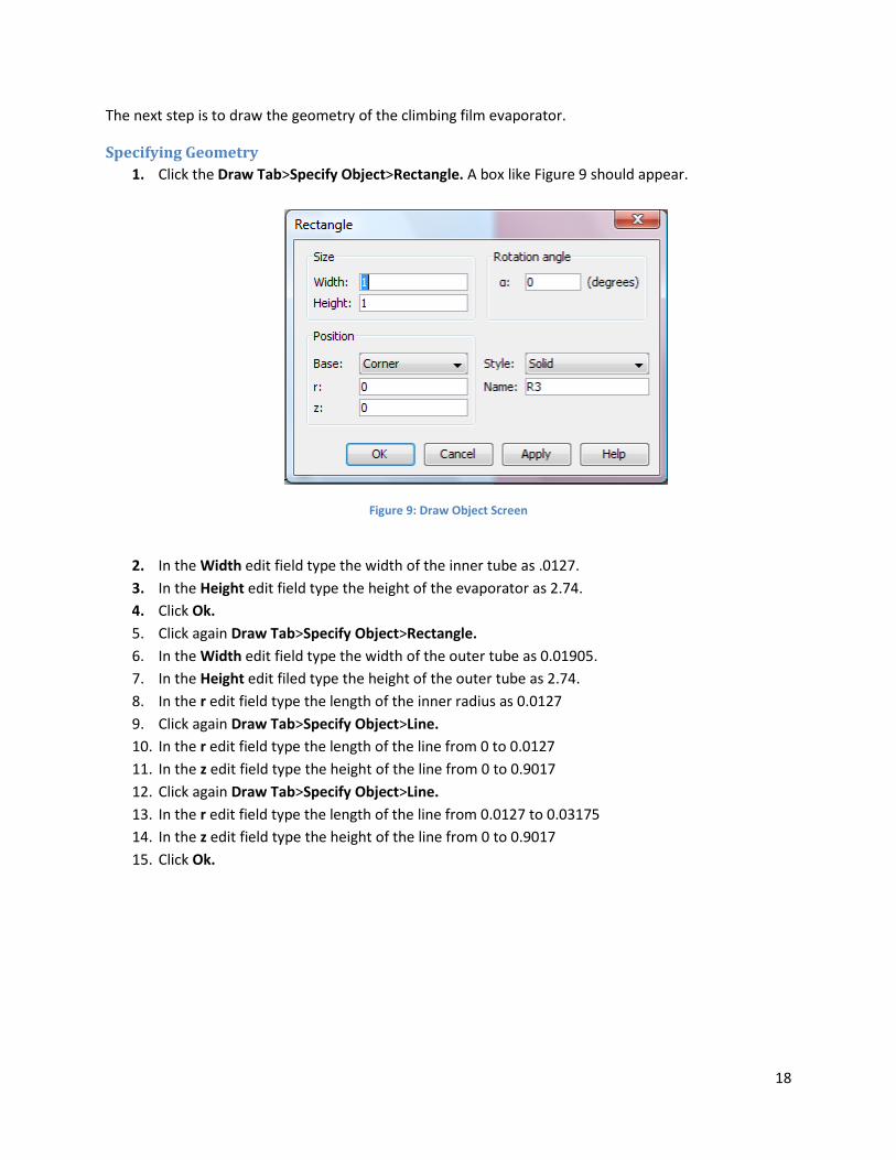
Specifying Geometry 1. Click the Draw Tab>Specify Object>Rectangle. A box like Figure 9 should appear.

Figure 9: Draw Object Screen

2. In the Width edit field type the width of the inner tube as .0127. 3. In the Height edit field type the height of the evaporator as 2.74. 4. Click Ok. 5. Click again Draw Tab>Specify Object>Rectangle. 6. In the Width edit field type the width of the outer tube as 0.01905. 7. In the Height edit filed type the height of the outer tube as 2.74. 8. In the r edit field type the length of the inner radius as 0.0127 9. Click again Draw Tab>Specify Object>Line. 10. In the r edit field type the length of the line from 0 to 0.0127 11. In the z edit field type the height of the line from 0 to 0.9017 12. Click again Draw Tab>Specify Object>Line. 13. In the r edit field type the length of the line from 0.0127 to 0.03175 14. In the z edit field type the height of the line from 0 to 0.9017 15. Click Ok.

19

The geometry should look like Figure 10.

Figure 10: Geometry

The dimensions of the climbing film evaporator were based on the actual size of the climbing film evaporator located in the Unit Operations Laboratory in Goddard Hall. We measured the height of the apparatus to be 9 feet, the inner tube radius to be 1 inch and the outer tube radius to be 2.5 inches. All values were converted to meters to agree with COMSOL since it uses the metric system.

The line that divides the evaporator represents the height at which boiling starts occurring under this particular conditions and it was determined experimentally at 0.9017 m.

20

The next step is to setup the constants and global expression that were used to model the experiment.

Constant set up 1. - Click the Options Tab>Constants and input the constants seen in Figure 10.

Figure 11: COMSOL Constants

Where D and Dg stand for water and gas diffusivity respectively and are in the units of m2/s. K is the thermal conductivity constant in W/K*m. Cp is the heat capacity of water in J/m*K. Rho is the density of the mixture and was measured in kg/m3. Ue is the heat transfer coefficient to the environment in W/ (m2K). Ul and Uu are the lower and upper heat transfer coefficients for the evaporator in W/ (m2K). Tf, Ts, Ta and Tb are the initial temperature of the mixture, the temperature

21

of the steam in the outer side, the ambient temperature and the boiling temperature of the mixture all in degrees Kelvin. Fr is the volumetric flow rate in ml/min. vin is the initial velocity of the feed and was calculated using the volumetric flow rate and has units of m/s. vst is the initial velocity of the steam in m/s. Cw0, Cg0 and Cwv0 are the initial concentrations of water, glycerol and water vapor in mol/m3 refer to appendix A for calculations. Lt is the total height of the evaporator in m. for purposes of modeling Ll is the height at which boiling occurs and Lu is the difference between the total height and the boiling height both in m. r1 and r2 are the inner tube radius and outer tube radius un m. lam is the heat of vaporization lambda in kJ/kg. saiu, sail, saou and saol are the inside upper surface area, inside lower surface area, outside upper surface area and outside lower surface area all in m2. Vuj and Vlj are the upper and lower volumes in m3.aiu, aou, ail and aol are surface areas over volume ratios used for modeling purposes all in m.

Expressions set up 1. Click the Options Tab>Expressions>Global Expressions and input the equations seen in Figure

12.

Figure 12: COMSOL Global Expressions

These expressions are used to calculate additional parameters that make the model function. Ql is the heat gained by the process from the steam in the lower part of the evaporator in watts. Qu is the heat gained by the process from the steam in the upper part of the evaporator in watts. Ql and Qu are necessary because we have to take into account that the upper and lower parts of the evaporator have different heat transfer coefficients due to the boiling that occurs inside the evaporator. Qe is the heat lost by the steam to the environment in watts. erate is the rate of vaporization of water inside the inner tube in mol/m3*s. Wg is the weight fraction of glycerol inside the inner tube. Qrate is the rate of heat lost by the upper part of the inner tube to the steam.

22

The next step is to set the physics of the model which include the subdomain settings and the boundary conditions settings.

Subdomain settings

Convection and Diffusion (chcd) 1. Select from the toolbar Multiphysics> 1 Convection and Diffusion (chcd). 2. Click from the toolbar Physics>Subdomain Settings. A box like Figure 13 should appear.

Figure 13: chcd Subdomain Settings

3. Select from the subdomain selection list subdomain 1. 4. Select from the tabs Cw. 5. Type D in the diffusion coefficient box and vin in the z-velocity box. 6. Select from the tabs Cg. 7. Type D in the diffusion coefficient box and vin in the z-velocity box. 8. Select from the tabs Cwv. 9. Type Dg in the diffusion coefficient box and vin in the z-velocity box. 10. Select from the tabs Init. 11. Type Cw0, Cg0 and Cwv0 in the initial concentrations boxes. 12. Select from the subdomain selection list subdomain 2. 13. Repeat steps 4 through 11. Additionally in step 5 type in the reaction rate box –erate and in

step 9 type in the reaction rate box erate.

In order to simplify the model we are treating the evaporation of water as a reaction. We are assuming that water in the liquid phase is disappearing (evaporating) at a rate equal to Uu*a*(Ts-Tb)/(lam*18)

23

and its appearing in the gas phase at the same rate. Hence the terms erate and –erate in the reaction rate boxes for Cw and Cwv.

Convection and Diffusion (chcc) 1. Select from the toolbar Multiphysics> 2 Convection and Diffusion (chcc). 2. Click from the toolbar Physics>Subdomain Settings. A box like Figure 14 should appear.

Figure 14: chcc Subdomain Settings

3. Select from the subdomain selection list subdomain 1. 4. Select from the tabs Physics. 5. Click the K (anisotropic) box in the upper left corner of the square type 6000 and in the lower

left right of the square type .006 as the thermal conductivities. Type rho in the density box. Type Cp in the heat capacity box and type vin in the velocity field box.

6. Select from the tabs init. 7. Type Tf as the initial temperature. 8. Select from the subdomain selection list subdomain 2. 9. Select from the tabs Physics. 10. Click the K (anisotropic) box in the upper left corner of the square type 6000 and in the lower

left right of the square type .006 as the thermal conductivities, type rho in the density box, type Cp in the heat capacity box, type –Qrate in the heat source box and type vin in the velocity field box.

11. Select from the tabs init. 12. Type Tb as the initial temperature. 13. Click OK.

24

For modeling purposes we are assuming that the mixture will maintain the same temperature once it starts boiling, we achieve this by implementing the term –Qrate in the upper part of the evaporator. Additionally, we make the thermal conductivity K in the r direction very big and K in the z direction very small. To ensure that all the resistance to heat transfer is lumped into the heat transfer coefficient that appears in the boundary condition.

Convection and Diffusion (chcc2) 14. Select from the toolbar Multiphysics> 3 Convection and Diffusion (chcc2). 15. Click from the toolbar Physics>Subdomain Settings. A box like Figure 14 should appear.

Figure 15: chcc2 Subdomain Settings

16. Select from the subdomain selection list subdomain 3. 17. Select from the tabs Physics. 18. Click the K (isotropic) box input 25000 as the thermal conductivity, type 0.6 in the density box,

type 2058 in the heat capacity box, type Ql*ail-Qe*aol in the heat source expression and type vst in the velocity field box.

19. Select from the tabs init. 20. Type Ts as the initial temperature. 21. Select from the subdomain selection list subdomain 4. 22. Select from the tabs Physics. 23. Click the K (isotropic) box input 25000 as the thermal conductivity, type 0.6 in the density box,

type 2058 in the heat capacity box, type Qu*aiu-Qe*aou in the heat source expression and type vst in the velocity field box.

24. Select from the tabs init. 25. Type Ts as the initial temperature.

25

26. Click OK.

For modeling purposes we are assuming that the steam running in the outer tube of the evaporator has uniform temperature. To model this behavior we decided to include the heat source terms in order to maintain the temperature of the steam as constant as possible.

Boundary settings

Convection and Diffusion (chcc) 1. Select from the toolbar Multiphysics> 2 Convection and Diffusion (chcd). 2. Click from the toolbar Physics>Boundary Settings. A box like Figure 16 should appear.

Figure 16: chcd Boundary Conditions

3. From the boundary selection list click boundary 1. 4. From the boundary condition drop down menu select Axial Symmetry. 5. From the boundary selection list click boundary 2. 6. From the boundary condition drop down menu select Concentration. 7. Click the concentration edit field and type Cw0 as the initial concentration. 8. Select from the tabs Cg. 9. From the boundary condition drop down menu select Concentration. 10. Click the concentration edit field and type Cg0 as the initial concentration. 11. Select from the tabs Cwv. 12. From the boundary condition drop down menu select Concentration. 13. Click the concentration edit field and type Cwv0 as the initial concentration. 14. From the boundary selection list click boundary 3. 15. From the boundary condition drop down menu select Axial Symmetry. 16. From the boundary selection list click boundary 5. 17. From the boundary condition drop down menu select Convective Flux. 18. From the boundary selection list click boundary 6. 19. From the boundary condition drop down menu select Insulation/symmetry.

26

20. From the boundary selection list click boundary 8. 21. From the boundary condition drop down menu select Insulation/symmetry. 22. Click OK.

The boundary conditions represent the physical phenomena occurring in every side of the rectangle. For this particular case, the boundary conditions specified correspond to the mixture inside the evaporator. Boundaries 1 and 3 are located on the axis of symmetry and are specified as such. Boundary 2 is where the mixture enters the evaporator and is denoted as Concentration. Boundary 5 is the exit of the evaporator and is specified as Convective Flux. Boundaries 6 and 8 are the side of the evaporator that is in contact with the steam and are specified as insulation/symmetry.

Convection and Diffusion (chcc) 1. Select from the toolbar Multiphysics> 2 Convection and Diffusion (chcc). 2. Click from the toolbar Physics>Boundary Settings. A box like Figure 17 should appear.

Figure 17: chcc Boundary Conditions

3. From the boundary selection list click boundary 1. 4. From the boundary condition drop down menu select Axial Symmetry. 5. From the boundary selection list click boundary 2. 6. From the boundary condition drop down menu select Temperature. 7. Select the Temperature edit field and type Tf. 8. From the boundary selection list click boundary 3. 9. From the boundary condition drop down menu select Axial Symmetry. 10. From the boundary selection list click boundary 4. 11. From the boundary condition drop down menu select Continuity. 12. From the boundary selection list click boundary 5. 13. From the boundary condition drop down menu select Convective Flux. 14. From the boundary selection list click boundary 6. 15. From the boundary condition drop down menu select Heat Flux.

27

16. Select the Inward Heat Flux edit field type in Ql. 17. From the boundary selection list click boundary 8. 18. From the boundary condition drop down menu select Heat Flux. 19. Select the Inward Heat Flux edit field type in Qu. 20. Click Ok.

These boundary conditions correspond to the physical phenomena interacting with the temperature in the inner tube of the evaporator. Boundaries 1 and 3 are located on the axis of symmetry. Boundary 2 is the initial temperature of the mixture entering the evaporator. Boundary 4 represents the height at which boiling starts occurring. Boundary 5 is the temperature of the mixture exiting the evaporator. Boundaries 6 and 8 represent the interaction between the temperature of the mixture in the inner tube with the temperature of the steam running in the outer tube of the evaporator.

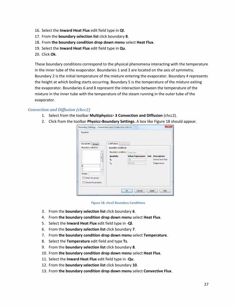
Convection and Diffusion (chcc2) 1. Select from the toolbar Multiphysics> 3 Convection and Diffusion (chcc2). 2. Click from the toolbar Physics>Boundary Settings. A box like Figure 18 should appear.

Figure 18: chcc2 Boundary Conditions

3. From the boundary selection list click boundary 6. 4. From the boundary condition drop down menu select Heat Flux. 5. Select the Inward Heat Flux edit field type in -Ql. 6. From the boundary selection list click boundary 7. 7. From the boundary condition drop down menu select Temperature. 8. Select the Temperature edit field and type Ts. 9. From the boundary selection list click boundary 8. 10. From the boundary condition drop down menu select Heat Flux. 11. Select the Inward Heat Flux edit field type in -Qu. 12. From the boundary selection list click boundary 10. 13. From the boundary condition drop down menu select Convective Flux.

28

14. From the boundary selection list click boundary 11. 15. From the boundary condition drop down menu select Heat Flux. 16. Select the Inward Heat Flux edit field type in Qe. 17. From the boundary selection list click boundary 12. 18. From the boundary condition drop down menu select Heat Flux. 19. Select the Inward Heat Flux edit field type in Qe. 20. Click Ok.

These boundary conditions correspond to the physical phenomena interacting with the temperature of the steam in the outer tube of the evaporator. Boundaries 6 and 8 represent the interaction between the temperature of the steam in the outer tube and the temperature of the mixture in the inner tube. Boundary 7 is the initial temperature if the steam. Boundary 10 is the outlet temperature of the steam at the top of the tube. Boundaries 11 and 12 represent the heat lost of the steam to the environment. The flow of steam out the top in the model does not correspond to the actual situation in the lab but helps maintain the steam temperature uniform in our model.

Extrusion coupling values In order to make the model work we have to define some extrusion coupling variables. For example, to implement a boundary condition with a temperature difference across the boundary, the value of temperature in both sides of the boundary needs to be solved within each subdomain. Thus the value of T on one side is stored in a new variable, Ti and extruded to the other side of the boundary.

1. Click from the toolbar Options>Extrusion Coupling Values>Subdomain Extrusion Values a screen like Figure 19 should be prompted.

Figure 19: Extrusion Coupling Values

2. From the Subdomain selection list select subdomain 1. 3. Under the Name edit field write the variable Ti and under the Expression edit field write the

variable T. 4. Click the Destination tab. 5. From the Subdomain selection list check 3. 6. Click the Source Vertices tab. 7. From the Vertex selection list select 1 and 2. 8. Click the Destination Vertices tab.

29

9. From the Vertex selection list select 4 and 5. 10. Click Ok.

Mesh Generation With all the components of the model defined and specified, the only thing left to solve the model is to specify the mesh criteria.

1. From the toolbar select Mesh>Refine Mesh three times. 2. From the toolbar select Solve>Solve Problem.

Postprocessing 1. From the toolbar select Postprocessing> Plot Parameters. Click on the Surface tab and type Wg en

the Expression edit field.

30

Results and Discussion

Part 1: Results for the Mass Balance on the Climbing Film Evaporator The summarized results of both the runs (evaporator running at 5psig steam pressure and evaporator running at 10 psig steam pressure) to concentrate a glycerol solution using a climbing film evaporator are presented in Tables 1 and 2. Detailed sample calculations are shown in Appendix A.

Feed Rate (kg/hr)

Mass Flow Rate of steam(kg/h)

Condenser Rate (kg/h)

Product Rate ( kg/h)

% glycerol in the product solution(measured)

7.37 7.5 3.3 4.07 16 12.2 8.1 2.7 9.585 13

18.4 9 2.4 16.027 11

24.6 9.3 1.8 22.77 10.5 Table 1: Calculated values for input and output flow rates and percentage glycerol in product @ 5 psig

Feed Rate (kg/hr)

Mass Flow Rate of steam(kg/h)

Condenser Rate (kg/h)

Product Rate ( kg/h)

% glycerol in the product solution(measured)

7.37 7.8 4.2 3.17 17 12.2 9 3.9 8.385 14 18.4 9.6 3.3 15.127 12 24.6 9.9 2.7 21.870 11

Table 2: Calculated values for input and output flow rates and percentage glycerol in product @ 10 psig

The tabular results presented above help us compare certain numerical values right away. We can see that as the steam pressure increases the flow rate of steam increases along with the condenser solution flow rates and percentage glycerol in the product. An important thing to note here is that as the steam pressure and flow rate increase the product solution flow rate decreases. The reason this happens is because as the steam flow rate increases more energy is given off by the steam which in turn helps to evaporate more water from the feed solution. Thus a higher quantity of water vapor is generated which then condenses and exits through the condenser solution leaving less water in the product stream resulting in a higher glycerol concentration. A graphical representation of the effect of higher steam pressure on the percentage glycerol in the product is shown below in Table 3.

Feed Flow Rate (kg/h) Mass of Glycerol @ 5 psig

Mass of Glycerol @ 10 psig

7.3 0.085736 0.198025 12.2 0.01755 0.054595 18.4 0.079723 0.027446 24.5 0.066149 0.051298

Table 3: Calculated values for percentage glycerol in the condenser solution

31

The values given in the table above where obtained by measuring the concentration of glycerol in the condensate and validate an important assumption that the condenser solution is considered to be 100% water with no or negligible glycerol present.

This assumption helps in calculating the mass balance and composition of the product solution and is generally used for climbing film evaporator calculations. The values given above are clearly very small with exception of the one at 7.3 kg/hr and 10psig. The deviation in this particular value can be attributed to human error while performing the mass balances or failing to attain steady state. The overall trend supports that it is right to assume there is no glycerol the condenser solution.

Figure 20: Experimental results comparing glycerol concentration in the product at different steam pressures

The main objective of this lab was to use the climbing film evaporator to increase the percentage of glycerol from 10 % in the feed solution to 16% or higher in the product solution .The graph above (figure 20) makes it very obvious that as the steam pressure is increased the concentration of glycerol in the product solution increases.

We can also deduce that at any given steam pressure when the feed flow rate is increased the percentage glycerol in the product decreases. This happens because when the steam pressure is held constant and feed flow rate is increased more of the heat transfer from the steam is required to heat the feed to the boiling point and less is available for evaporation. The energy provided by the heat to the process does increase and the condensate flow rate also increases, but since the feed is flowing at a higher rate the contact time between the feed and the steam decreases. This results in less water (than should have actually evaporated had the flow rate not increased by a big margin) being evaporated and ending up in the product stream which gets diluted. Heat given off by the steam is calculated by:

𝑄𝑄𝑆𝑆 = �̇�𝑐𝑑𝑑𝜆𝜆𝑑𝑑

10

11

12

13

14

15

16

17

18

7 12 17 22

Perc

enta

ge G

lyve

rol

Feed Flow Rate (kg/h)

5 psig

10 psig

32

Mathematically as �̇�𝑐𝑓𝑓 increases �̇�𝑐𝑑𝑑 and hence 𝑄𝑄𝑆𝑆 also increase but not enough to increase �̇�𝑐𝐴𝐴, meaning

feed flow rate has a larger effect on evaporation rate than condensate flow rate. This problem can be solved by increasing the height of the evaporator so that there is enough contact time and area for the steam to vaporize more water.

According to the results above for our given tube height and surface area we need to run the evaporator at a high steam pressure and low flow rates to obtain a more concentrated product.

Comparison to Theoretical Data

Figure 21: Comparison of experimental and theoretical percentage of glycerol in the product @10 psig

The experimental data obtained for the percentage of glycerol in the produt solution was compared to the theoretical values of percentage glycerol in the product. Detailed information and calculations infromation regarding the theoretical values are given in Apppendix A. The graph above compares the theoretical and experimental values at a steam pressure of 10 psig. The trend for both experimental and theoretical curves seems to be the same i.e the percentage glycerol of the product goes down as the feed flow rate increases as stated earlier. However, the theoretical curve is slightyl higher than the experimental curve in most cases which leads us to conclude that the slight difference in values can be attributed to various experimental errors such as mistakes in reading the percentages off the specific gravity chart, mistakes in measuring the condensate flow rate etc. The first experimental data point (17%) is however much lower than the theoretical value (23%). This large difference is most possibly due to the fact that the measurements were made before the evaporator systeam had attained steady state. If this is the case then the heating and vaporization in the tube had not yet become uniform resulting in uneven sloshing over of liquid into the product stream corrupting the data measurements. The solution to this is to wait longer for the system to come to steady state and figure out a way to estimate the time required for that so that measurements are made at proper intervals.

11

13

15

17

19

21

23

25

6 8 10 12 14 16 18 20 22 24

% G

lyce

rol i

n th

e co

nc s

oln

Feed Flow Rate (kg/h)

Experimental

Theoretical

33

Part 2: Results for the Energy Balance on the Climbing Film Evaporator

The values in the table above help us to directly compare 𝑄𝑄𝑝𝑝 and 𝑄𝑄𝐸𝐸 at different steam pressures and as

the feed flow rate increases. We can see that as the feed flow rate increases the heat gained slightly increases indicating that as more solution is fed into the more energy is gained by it. However, as it was stated earlier that when the feed flow rate increases vaporization of water does increase but not a lot since the residence time of the solution in the evaporator tube decreases. Similarly heat gained by the process does increases but not by a big margin since the residence time gets shorter.

Figure 22: Trend followed by QP at variable steam pressures

When the steam pressure is increased and a similar pattern of flow rates are used the energy gained by the process increases. This result is intuitive since we know that when steam pressure increases the

2000

2200

2400

2600

2800

3000

3200

7 12 17 22

Ener

gy g

aine

d by

the

pro

ces(

Wat

ts)

Feed flow Rate( kg/h)

QP at 5psig

QP at 10 psig

Steam Pressure (psig)

Feed Flow Rate (kg/h)

Heat gained by the process Qp(kW)

Heat loss to the environment QE (kW)

5 7.3710 2.0659 3.7011 5 12.285 2.1977 4.0325 5 18.427 2.5689 4.3531 5 24.570 2.8030 4.3501

10 7.3710 2.47947 3.52 10 12.285 2.75088 4.1716 10 18.427 2.98725 4.3967 10 24.570 3.2275 4.3873

Table 4: Calculated values for heat gained by the process and heat lost to the environment at variable steam pressures.

34

condensate flow rate increases. The reason for this is that at a higher steam pressure the heat transfer to the process fluid changes to use more heat from the available steam. Changing or increasing the steam pressure at a given feed flow rate results in a higher condensate flow rate because the driving force for heat transfer in the evaporator (Ts-Tp) and (Ts-Ta) increases with an increase in pressure. This trend is depicted in Figure 22 above.

On the other hand as the feed flow rate is increased, the condensate (steam) flow rate also increases and thus the energy available increases. Since only a small fraction of this excess energy is gained by the process, a chunk of this energy is lost to the environment due to lack of insulation, conduction through the glass tube etc. Hence the heat lost to the environment also increases slightly with an increase in the feed flow rate and for practical purposes is considered to be more or less constant. As the operating pressure of the steam being supplied is increased the energy gained by the process increases since steam at a higher pressure has a higher temperature and therefore more heat energy available. Similarly heat lost to the environment also increases as the steam pressure is increased. This trend is depicted in Figure 23 below.

Figure 23: Trend followed by QE for variable steam pressure and feed flow rate

We can see from the graph above that the QE at 10 psig is higher than QE at 5 psig in three of the four data points which agrees with the above explanation. However, for the very first data point (lowest flow rate) the heat loss is higher at 5 psig. This is an anomaly and should not be the case and the possible explanation for this deviation from the trend is that at 5 psig the process had not yet reached steady state when we made the measurements and recorded the data. When the system is not at steady state there is uneven heating and vaporization of water which results in erratic energy lost and energy utilized values.

3400

3600

3800

4000

4200

4400

4600

7 9 11 13 15 17 19 21 23 25

Ener

gy lo

st t

o th

e en

viro

nmen

t(W

atts

)

Feed flow Rate( kg/h)

QE at 5psig

QE at 10 psig

35

Comparison of QP and QE For a constant flow rate and constant steam pressure 𝑄𝑄𝐸𝐸 is higher than 𝑄𝑄𝑃𝑃 and is illustrated in the Figure 24 below.

Figure 24: Comparison of QP and QE with varying flow rates at 5 psig

This indicates that our climbing film evaporator is thermally inefficient. The reason for this is that our evaporator is not insulated and made of glass. This has been done to enable users to see the process through the glass walls. If the evaporator was insulated which most of them generally are, the heat loss to the environment would have been lesser and the evaporator would be more efficient.

Part 3: Overall Heat Transfer Coefficient Results One objective of the experiment was to determine how the glass and the atmosphere offer resistance to heat transfer from steam to the feed solution. An outer heat transfer coefficient would be the measure of the resistance that the air and glass present to transfer of heat from the steam to the environment. This was calculated considering the entire tube as a whole and the results are presented in Figure 25 below.

1500

2000

2500

3000

3500

4000

4500

5000

7 12 17 22

Hea

t gai

ned

by t

he p

roce

ss Q

P (W

)

Feed Flow Rate (kg/h)

QE

QP

36

Figure 25: Comparison of Ue at variable steam pressures

From the graph above we can deduce that the outer heat transfer coefficient increases initially with the feed flow rate and starts to level out towards the higher flow rates. The trend is almost identical for both steam pressures indicating that the resistance to heat transfer increases with increasing feed flow rate. The outer heat transfer coefficient is higher for the lower steam pressure indicating that there is a higher resistance offered by glass and a layer (film) of air on the outer side of the glass tub to the flow of heat energy from the steam to the environment and vice versa. Although more heat is lost to the environment at the higher steam pressure, the driving force is also larger resulting in Ue at higher pressure being less than Ue at lower pressure according to the relation below.

𝑈𝑈 =𝑄𝑄

𝐴𝐴 ∗ 𝛥𝛥𝛥𝛥

However the evaporator should be run at a 5 psig since there is less quantitative heat loss at lower pressures.

For the case of the inner overall heat transfer coefficient the evaporation process was broken into two parts. First, where the feed solution gains heat to start boiling was considered the lower part of the tube which has a separate heat transfer coefficient involving a temperature driving force raises the feed from its initial temperature to the boiling point of water. The second part is the process of conversion of the boiling solution to water vapor. This was called the upper part of the process and called the upper heat transfer coefficient which includes the driving force that pushes the temperature of the solution from boiling point of water to the outlet temperature at which the vapor exits the evaporator tube.

The results for the lower heat transfer coefficient for the two different steam pressures are presented in Figure 26 below.

1300

1400

1500

1600

1700

1800

1900

5 10 15 20 25

Ove

rall

Out

er U

(W/m

^2.K

)

Feed Flow Rate (kg/h)

5psig

10psig

37

Figure 26: Comparison of the Ulower at different steam pressures

The overall lower heat transfer coefficient is lower for lower steam pressure, a trend which is the complete opposite of the outer heat transfer coefficient. The explanation for this result is that at higher P we have higher Ts so (Ts-Ta) is higher so we get more steam condensate. This increased steam condensate runs down the glass wall and provides more resistance to heat transfer between the steam and the process fluid thus making Ul increase with increasing pressure. All these factors indicate that less heat is being transferred to the solution due to convective resistances resulting in an increase in the overall heat transfer coefficient for a higher pressure.

The lower heat transfer coefficients for both steam pressures show an increase with increasing feed flow rate. This trend is due to the fact that the boundary layer that offers the main resistance inside the tube gets smaller with increasing velocity thereby increasing the lower heat transfer coefficient as the feed flow rate increases. This explanation is supported by Figure 26 except for the value at the highest feed flow rate at 5 psig which dips unexpectedly. This could be due to experimental error possibly an error in the measurement of the boiling height for the lower tube since even a difference of 5 inches in the boiling height changes the heat transfer coefficient by around a 100 W/m2.K.

And just like the case above the upper heat transfer coefficient at the higher steam pressure is higher indicating the resistance to heat transfer also increases as we increase the steam pressure. This result is also expected due to the well known fact predicted by the Dittus Boelter equation that heat transfer coefficient increase with increasing fluid velocity. However, the upper heat transfer coefficients in our case don’t exactly follow this prediction very well due to violent and erratic slugging-walls not wetted uniformly. This result is illustrated on Figure 27 below.

700

750

800

850

900

950

1000

1050

1100

1150

5 10 15 20 25 30

Low

er O

vera

ll U

(W/m

^2.K

)

Feed Flow Rate(kg/h)

U lower 10 psig

Ulower at 5psig

38

Figure 27: Comparison of the U(upper) at different steam pressures

The trends for this graph are also more or less constant only increasing within a small range indicating that the heat transfer coefficient doesn’t change much with an increase in the feed flow rate however the operating pressure of steam has a significant effect on both the upper and lower heat transfer coefficients as raising the pressure by 5 psig increases U lower and U upper by a magnitude of around 100 W/m2.K. Both Ul and Uu are lower at lower steam pressure because of slight T dependence of viscosity and other factors that influence a heat transfer coefficient and usually make them increase slightly with higher pressure.

Comparison of U lower and U upper

Figure 28: Comparison of U lower and U upper at 10 psig

400

420

440

460

480

500

520

540

560

580

600

5 10 15 20 25 30

Upp

er U

(W/m

^2.K

)

Feed Flow Rate (kg/h)

U upper 10 psig

U upper at 5psig

400

500

600

700

800

900

1000

1100

1200

5 10 15 20 25 30

U lower 10 psig

Uupper at 10psig

39

As already evident by Figure 26 and 27 both the upper and lower heat transfer coefficients show a slight variation (numerical increase) with an increased feed flow rate however this increase not so significant and they can be considered more or less constant as illustrated by Figure 28 above.

Part 4: Results for Evaporator Economy and Capacity

The success of any process is totally dependent on a cost-benefit analysis. If the cost of the process exceed the profit then the process is considered to be inefficient and uneconomic and if the benefits are higher than the costs the process if considered to be beneficial and efficient. The results of evaporator capacity are presented in Figure 29 below.

Figure 29: Evaporator Economy at variable steam pressures

The graph above illustrates that as the feed flow rate increases the evaporator capacity decreases which makes sense since capacity is directly the measure of the amount of water evaporated from the feed solution. As discussed earlier the condenser solution flow rate decreases with increased feed flow due to smaller contact time between steam and feed and also because it takes more energy and surface area to heat the feed to the boiling point when there is more feed to be heated. The capacity however increases as the steam pressure is increased (agrees with the results of condenser solution flow rate) as discussed in Section 1 Table 1 and 2.

The most important measure of the success of the evaporator is its economy and as stated earlier our evaporator would be more efficient if it was insulated. The results of evaporator economy are discussed below in Figure 30.

1

1.5

2

2.5

3

3.5

4

4.5

5 10 15 20 25 30

Evap

orat

or C

apac

ity

Feed Flow Rate (kg/h)

5 psig

10 psig

40

Figure 30: Evaporator Economy at variable steam pressures

The graph above indicates that just like capacity evaporator economy also decreases with an increase in feed flow rate. The economy is higher for a higher steam pressure compared to a lower steam pressure. This can be explained by the fact that at higher flow rates less water is being vaporized and therefore the product solution is less concentrated and at higher steam pressures and constant flow rate more water is vaporized from the feed solution resulting in a more concentrated product.

In conclusion, the way to elicit the best performance from the climbing film evaporator is to operate it at low flow rates and high pressure as this would result in a more concentrated result and better economy. The flip side is that we have to operate the evaporator for longer times since it takes longer for the process to attain steady state at lower flow rates. This will also result in a higher resistance to heat transfer in the form of higher heat transfer coefficients at higher pressures. In the end a balance has to be maintained between operating time and energy and product specifications and economy.

0.1

0.15

0.2

0.25

0.3

0.35

0.4

0.45

0.5

0.55

0.6

5 10 15 20 25 30

Evap

orat

or E

cono

my

Feed Flow Rate(kg/h)

5 psig

10 psig

41

Part 5: COMSOL Modeling Results

Material balance results From Figure 31 we can see the concentration of glycerol throughout the length of the climbing film evaporator. The mixture enters at the bottom of the evaporator with a concentration of 10 percent glycerol in water and exits at the top with a concentration of 12.8 percent glycerol in water. In accordance with the behavior seen in the experimental run, we can see from Figure 32 that the concentration of glycerol in the solution starts increasing only once it reaches the boiling temperature of water, which is attained at the boiling height in the tube denoted by the horizontal line in Figure 31. Our experimental data showed an entering mixture composition of 10 percent glycerol in water and an exit composition of 12 percent glycerol in water. Thus, we can conclude that the results from the lab experiment and COMSOL model are comparable.

Figure 31: Concentration of glycerol throughout the length of the climbing film evaporator

42

Figure 32: Glycerol in water concentration profile

Energy balance results Using COMSOL boundary integration we solved for the total heat given by the steam and using formula [7] we solved for the steam trap flow rate. Results are presented in table 5.

The results suggest that there is a 22% error in the total heat given in the steam. We speculate that the reason for an error this large is because COMSOL models the experiment ideally whereas in real life there could be a leak from the steam to the environment or the ambient temperature could be higher or lower than what we specified in COMSOL. The percent error in the steam trap flow was only 5%. Thus, we concluded that by finding better heat transfer coefficients to use in the COMSOL model we can simulate the experiment with more accuracy.

COMSOL Experimental %Error

Qs (W) 5758.36 7384 -0.22016

Ws (Kg/s) 9.1 9.6 -0.05208

Table 5: Experimental and COMSOL results Qs and Ws

43

Figure 33 represents the temperature profile of the mixture inside the inner tube with respect to the height of the evaporator. The graph illustrates how the temperature of the mixture inside the inner tube increases exponentially until reaching the boiling height measured at 0.9017m. The temperature then levels off and remains constant at 372.8 Kelvin. This result agrees with the fact that temperature doesn’t increase when there is a phase change.

Figure 33: Temperature profile

Heat Transfer Coefficient Results Table 6 presents the heat transfer coefficients used in COMSOL and the ones calculated in the experiment.

COMSOL Experimental

Uu (W/K*m2 ) 800 503

Ul (W/K*m2 ) 500 1093 Table 6: Experimental and COMSOL Heat Transfer Coefficients

The variables used for COMSOL are adjustable but this particular set of values provided a reasonable match with the experimental glycerol concentration. The large difference between the COMSOL and the experimental heat transfer coefficients might be because COMSOL models the experiment ideally. Additionally, in the experiment there is the formation of a liquid film caused by the condensation of water in the steam side that affects significantly the upper heat transfer coefficient causing it to decrease. In COMSOL this behavior is not modeled.

44

Conclusions Based on our results from the experiment we can conclude that as we increase the operating

steam pressure the flow rate of the product stream decreases however the concentration of glycerol in the product stream increases. The concentration of the glycerol in the product decreases with an increase in the feed flow rate. Hence we can safely conclude that in order to get the highest possible product concentration we should run the evaporator on high steam pressure and low feed flow rates. Our results also validated the assumption that the condenser solution is in its totality water with negligible glycerol present. We also concluded that the concentration profile for glycerol in the product obtained experimentally is in accordance with theoretical predictions expected for the run at 120 ml/min. This anomaly was attributed the system not being at steady state when the data was recorded.

From our energy balance results we concluded that the heat gained by the process as well as the heat lost to the environment both increased slightly with an increase in steam pressure and feed flow rate. We concluded that the heat gained by the process shows a linear increase at both steam pressures whereas the energy lost to environment showed an increase for the initial flow rates and then levels out at the higher flow rates.

From our heat transfer coefficient results we concluded that the overall outer heat transfer coefficient increases initially and levels out at the end for the higher feed flow rates. This seems to be the trend at both operating steam pressures however the outer heat transfer coefficient is higher for the lower steam pressure leading us to assume that there is a lower resistance offered by the steam film formed on the glass surface to the flow of heat energy form steam to the environment. At the lower pressure less steam condenses resulting in a thinner film which offers less resistance to heat transfer compared to the higher pressure. The overall lower as well as upper heat transfer coefficients increase with an increase of steam pressure which leads to the conclusion that as the steam flow rate and pressure increase the size of the steam film on the wall increases which results in a higher resistance being offered to the flow of heat. Both the inner heat transfer coefficients show an increase with an increase in the feed flow rate however this change is very small and they can be considered reasonably constant over our range of feed flow rates. We also concluded that the inner heat transfer coefficients are very sensitive to the height at which the phase change in the feed occurs. Even a change of five inches in this height can change the coefficients by an order of magnitude of 102.

From the evaporator performance results we can conclude that the evaporator capacity decreases with an increase in the feed flow rate due to the reduced contact time between steam and the feed solution. The capacity increases with increasing steam pressure. The most important measure of the performance of the evaporator is the evaporator economy. We concluded that the evaporator economy decreases with an increase in feed flow rate and increases with an increasing operating steam pressure. This conclusion validates our first assumption that in order to get the best results we should run the evaporator at lower feed flow rates and higher operating steam pressures. For the feed rate of 300 ml/min, COMSOL approximated very well predicting a product concentration of 12.8 percent glycerol in water whereas in the experiment the measured concentration was 12 percent. The energy balance results did not match that closely with COMSOL reporting 5758 W of heat given by the steam whereas in the experiment the calculated heat given by the steam was 7384 W. We attribute this difference to the fact that COMSOL models the experiment ideally whereas in the actual experiment there could have been factors such as a leak from the steam to the environment that

45

could have affected the calculations. The temperature profile of the feed generated by COMSOL matched well with the profile predicted in our calculations. There was not a good agreement between the lower heat transfer coefficients calculated in the experiment and COMSOL. We believe this difference is due to the fact that in the experiment a thin film liquid forms on the glass wall caused by the condensation of water in the steam side that affects significantly the upper heat transfer coefficient causing it to decrease. In COMSOL this behavior is not modeled. Based on our COMSOL results and the experimental data, we can conclude that COMSOL can be an effective way for simulating a climbing film evaporator given the correct heat transfer coefficients, heat flux expressions, boundary conditions, and concentrations.

Recommendations The accuracy of the data obtained from this experiment can be increased by implementing new process conditions or changing some preexisting ones. First, more time should be allowed for each run to attain steady state. We waited 20 minutes for each run before recording the data. Although, this time might have been enough for some runs it might have been insufficient for others. We recommend future experimenters to measure the concentration of glycerol in the product every 10 minutes and once the concentration stops changing steady state would have been attained for sure. We also recommend doing additional runs using more feed flow rates and steam pressures in order to verify the trends shown by data. The model that was generated on COMSOL was a basic simulation of the evaporator process. In reality the climbing film evaporator is a complex unit operation. For simplicity in our model we specified the height at which the feed boils instead of asking COMSOL to model it. We also provided the upper and lower heat transfer coefficients instead of letting the model calculate these according from the process conditions that we input. For future models we suggest to find ways of making COMSOL calculate the heat transfer coefficients and the boiling height.

46

References

[1] McCabe, W. L., Smith, J. C. & Harriott, P. (2005). Unit Operations of Chemical Engineering (7th edition). In (E. D. Glandt, M. T. Klein & T. F. Edgar, Eds.). USA: Mc-Graw Hill.

[2] Minton, Paul.E. (1986). Handbook of Evaporation Technology. ( 1st edition). Noyes Publication. Park Ridge, New Jersey.

[3] Ribiero, C.P & Andrade Cano M.H.(2001). A heat transfer model for the steady-state simulation of climbing –falling –film plate evaporators. Journal of Food Engineering. Pages 309-320.

[4] Pacheco, C.R.F & Frioni L.S.M. (2001=3). Experimental results for evaporation of sucrose solution using a climbing film evaporator. Journal of Food Engineering. Pages 471-480.

[5] Young, B.R & Allen, R.M (1995) Multi-Input, Multi Output Identification of a Pilot- Plant Climbing Film Evaporator. Control Engineering Practice. Pages 1067-1-73

[6] Glover, William B. (2004). Chemical Engineering Progress- Selecting Evaporators for Process Applications. AIChE Journal. Pages 26-33.

[7] Sheikholesami, Roya., Yu, Hong, Doherty, William.(2004).Flow Boiling Heat Transfer of Water and Sugar Solutions in an Annulus. AIChE Journal Vol 50, No. 6. Pages 1119-1-1128.

[8] Haiyuan Biological. Rising thin film evaporator. Retrieved on April 24, 2010, from http://www.wxhysh.com/products/prod12.htm

[9] Author Stream. Evaporation. Retrieved on April 27, 2010, from http://www.authorstream.com/Presentation/jitpatel21-352080-evaporation-science-technology-ppt-powerpoint/

[10] Genemco. Aloe Vera Processing Equipment- Rising Film Evaporator. Retrieved on April 28, 2010, from http://www.genemco.com/aloe/rising.html

[11] Filter Machinec Manufacturers. Water Distillers. Retrieved on April 28, 2010, from http://www.filters-machines.com/water-distillers.html

[12] De Dietrich Process Systems. Evaporation-Climbing Film and Natural Circulation Evaporator. Retrieved on April 27, 2010, from http://www.ddpsinc.com/TeachingUnits/qts4.html

[13] COMSOL Multiphysics. Chemical Engineering Module-Water Treatment. Retrieved on April 25, 2010, from http://www.comsol.com/products/chem/

47

Appendices

Appendix A- Sample Calculations

Sample Calculations for Mass Balance

To calculate the mass balance we first need the mass flow rate of the feed solution. Since we measured the flow rate of the feed using a flow meter, it is in the units of ml/min and we need to convert it to kg/h. The first step to achieve this is to find the density of the feed solution. Since the solution is a mixture of water and glycerol, the density of this solution will be a combination of the densities of water and glycerol. The calculations are as follows:

𝐷𝐷𝑓𝑓𝑑𝑑𝑑𝑑𝑑𝑑𝑑𝑑𝐺𝐺 𝑜𝑜𝑓𝑓 𝐺𝐺𝐺𝐺𝐺𝐺𝑐𝑐𝑓𝑓𝐴𝐴𝑜𝑜𝐺𝐺 𝐴𝐴𝑑𝑑 25𝑜𝑜𝐶𝐶 (𝜌𝜌𝐺𝐺𝐺𝐺𝐺𝐺 ) = 1.261𝑔𝑔𝑐𝑐𝑐𝑐3

% 𝑜𝑜𝑓𝑓 𝐺𝐺𝐺𝐺𝐺𝐺𝑐𝑐𝑓𝑓𝐴𝐴𝑜𝑜𝐺𝐺 𝑑𝑑𝑑𝑑 𝑑𝑑ℎ𝑓𝑓 𝑓𝑓𝑓𝑓𝑓𝑓𝑓𝑓 𝑑𝑑𝑜𝑜𝐺𝐺𝑠𝑠𝑑𝑑𝑑𝑑𝑜𝑜𝑑𝑑 (𝑥𝑥𝑓𝑓) => 10% = 0.1

𝐷𝐷𝑓𝑓𝑑𝑑𝑑𝑑𝑑𝑑𝑑𝑑𝐺𝐺 𝑜𝑜𝑓𝑓 𝑊𝑊𝐴𝐴𝑑𝑑𝑓𝑓𝐴𝐴 𝐴𝐴𝑑𝑑 25𝑜𝑜𝐶𝐶 (𝜌𝜌𝑤𝑤 ) = 0.9974𝑔𝑔𝑐𝑐𝑐𝑐3

% 𝑜𝑜𝑓𝑓 𝑊𝑊𝐴𝐴𝑑𝑑𝑓𝑓𝐴𝐴 𝑑𝑑𝑑𝑑 𝑑𝑑ℎ𝑓𝑓 𝑑𝑑𝑜𝑜𝐺𝐺𝑠𝑠𝑑𝑑𝑑𝑑𝑜𝑜𝑑𝑑 (𝑥𝑥𝑓𝑓𝑤𝑤 ) => ( 1 − 0.1) = 0.9

𝐷𝐷𝑓𝑓𝑑𝑑𝑑𝑑𝑑𝑑𝑑𝑑𝐺𝐺 𝑜𝑜𝑓𝑓 𝑑𝑑ℎ𝑓𝑓 𝑑𝑑𝑜𝑜𝐺𝐺𝑠𝑠𝑑𝑑𝑑𝑑𝑜𝑜𝑑𝑑 �𝜌𝜌𝑓𝑓𝑓𝑓𝑓𝑓𝑓𝑓 � = (𝜌𝜌𝐺𝐺𝐺𝐺𝐺𝐺 ∗ 𝑥𝑥𝑓𝑓𝑔𝑔𝐺𝐺𝐺𝐺 ) + (𝜌𝜌𝑤𝑤 ∗ 𝑥𝑥𝑓𝑓𝑤𝑤 )

𝐷𝐷𝑓𝑓𝑑𝑑𝑑𝑑𝑑𝑑𝑑𝑑𝐺𝐺 𝑜𝑜𝑓𝑓 𝑑𝑑ℎ𝑓𝑓 𝑑𝑑𝑜𝑜𝐺𝐺𝑠𝑠𝑑𝑑𝑑𝑑𝑜𝑜𝑑𝑑 �𝜌𝜌𝑓𝑓𝑓𝑓𝑓𝑓𝑓𝑓 � = (1.261 ∗ 0.1) + (0.9974 ∗ 0.9) = 𝟏𝟏.𝟎𝟎𝟎𝟎𝟎𝟎𝟎𝟎𝟎𝟎 𝑔𝑔𝑐𝑐𝑐𝑐3

Calculating the Mass Flow Rate of the Feed:

𝑉𝑉𝑜𝑜𝐺𝐺𝑠𝑠𝑐𝑐𝑓𝑓𝑑𝑑𝐴𝐴𝑑𝑑𝑐𝑐 𝐹𝐹𝐺𝐺𝑜𝑜𝑤𝑤 𝑅𝑅𝐴𝐴𝑑𝑑𝑓𝑓 𝑜𝑜𝑓𝑓 𝑑𝑑ℎ𝑓𝑓 𝐹𝐹𝑓𝑓𝑓𝑓𝑓𝑓 (𝑉𝑉)̇ = 300𝑐𝑐𝐺𝐺𝑐𝑐𝑑𝑑𝑑𝑑

𝐷𝐷𝑓𝑓𝑑𝑑𝑑𝑑𝑑𝑑𝑑𝑑𝐺𝐺 𝑜𝑜𝑓𝑓 𝑑𝑑ℎ𝑓𝑓 𝑑𝑑𝑜𝑜𝐺𝐺𝑠𝑠𝑑𝑑𝑑𝑑𝑜𝑜𝑑𝑑 �𝜌𝜌𝑓𝑓𝑓𝑓𝑓𝑓𝑓𝑓 � = 1.02376

𝑀𝑀𝐴𝐴𝑑𝑑𝑑𝑑 𝐹𝐹𝐺𝐺𝑜𝑜𝑤𝑤 𝑅𝑅𝐴𝐴𝑑𝑑𝑓𝑓 𝑜𝑜𝑓𝑓 𝑑𝑑ℎ𝑓𝑓 𝐹𝐹𝑓𝑓𝑓𝑓𝑓𝑓 (�̇�𝑐𝑓𝑓) = �̇�𝑉 ∗ 𝜌𝜌𝑓𝑓𝑓𝑓𝑓𝑓𝑓𝑓

𝑀𝑀𝐴𝐴𝑑𝑑𝑑𝑑 𝐹𝐹𝐺𝐺𝑜𝑜𝑤𝑤 𝑅𝑅𝐴𝐴𝑑𝑑𝑓𝑓 𝑜𝑜𝑓𝑓 𝑑𝑑ℎ𝑓𝑓 𝐹𝐹𝑓𝑓𝑓𝑓𝑓𝑓 ��̇�𝑐𝑓𝑓� = 300 𝑐𝑐𝐺𝐺 𝑐𝑐𝑑𝑑𝑑𝑑

∗ 1.02376𝑔𝑔𝑐𝑐𝑐𝑐3 ∗

𝑐𝑐𝑐𝑐3

𝑐𝑐𝐺𝐺= 307.128

𝑔𝑔𝑐𝑐𝑑𝑑𝑑𝑑

𝑀𝑀𝐴𝐴𝑑𝑑𝑑𝑑 𝐹𝐹𝐺𝐺𝑜𝑜𝑤𝑤 𝑅𝑅𝐴𝐴𝑑𝑑𝑓𝑓 = 204.752𝑔𝑔𝑐𝑐𝑑𝑑𝑑𝑑

∗60 𝑐𝑐𝑑𝑑𝑑𝑑 ∗ 𝑘𝑘𝑔𝑔1000 𝑔𝑔 ∗ ℎ

= 18.427𝑘𝑘𝑔𝑔ℎ

𝑀𝑀𝐴𝐴𝑑𝑑𝑑𝑑 𝑜𝑜𝑓𝑓 𝑔𝑔𝐺𝐺𝐺𝐺𝑐𝑐𝑓𝑓𝐴𝐴𝑜𝑜𝐺𝐺 𝑑𝑑𝑑𝑑 𝑑𝑑ℎ𝑓𝑓 𝑓𝑓𝑓𝑓𝑓𝑓𝑓𝑓 �𝑐𝑐𝑓𝑓𝑔𝑔𝐺𝐺𝐺𝐺 � = 0.10 ∗ 12.285𝑘𝑘𝑔𝑔ℎ

= 1.8427𝑘𝑘𝑔𝑔ℎ

𝑀𝑀𝐴𝐴𝑑𝑑𝑑𝑑 𝑜𝑜𝑓𝑓 𝑤𝑤𝐴𝐴𝑑𝑑𝑓𝑓𝐴𝐴 𝑑𝑑𝑑𝑑 𝑑𝑑ℎ𝑓𝑓 𝑓𝑓𝑓𝑓𝑓𝑓𝑓𝑓�𝑐𝑐𝑓𝑓𝑤𝑤 � = 0.90 ∗ 12.285 = 16.585𝑘𝑘𝑔𝑔ℎ

48

Calculating the Mass Flow Rate of the Condenser Solution:

𝑀𝑀𝑓𝑓𝐴𝐴𝑑𝑑𝑠𝑠𝐴𝐴𝑓𝑓𝑓𝑓 𝑀𝑀𝐴𝐴𝑑𝑑𝑑𝑑 𝐹𝐹𝐺𝐺𝑜𝑜𝑤𝑤 𝑅𝑅𝐴𝐴𝑑𝑑𝑓𝑓 𝑜𝑜𝑓𝑓 𝑑𝑑ℎ𝑓𝑓 𝑐𝑐𝑜𝑜𝑑𝑑𝑓𝑓𝑓𝑓𝑑𝑑𝑑𝑑𝐴𝐴𝑑𝑑𝑓𝑓(�̇�𝑐𝐴𝐴) = 55𝑔𝑔𝑐𝑐𝑑𝑑𝑑𝑑

𝑀𝑀𝐴𝐴𝑑𝑑𝑑𝑑 𝐹𝐹𝐺𝐺𝑜𝑜𝑤𝑤 𝑅𝑅𝐴𝐴𝑑𝑑𝑓𝑓 𝑜𝑜𝑓𝑓 𝑑𝑑ℎ𝑓𝑓 𝑐𝑐𝑜𝑜𝑑𝑑𝑓𝑓𝑓𝑓𝑑𝑑𝑑𝑑𝐴𝐴𝑑𝑑𝑓𝑓(�̇�𝑐𝐴𝐴) = 180𝑔𝑔𝑐𝑐𝑑𝑑𝑑𝑑

∗60 𝑐𝑐𝑑𝑑𝑑𝑑 ∗ 𝑘𝑘𝑔𝑔1000 𝑔𝑔 ∗ ℎ

= 3.3𝑘𝑘𝑔𝑔ℎ

Calculating the Mass Flow Rate of the Concentrated Glycerol Solution (Product): (with 12 % glycerol concentration)

𝑀𝑀𝐴𝐴𝑑𝑑𝑑𝑑 𝑓𝑓𝐺𝐺𝑜𝑜𝐴𝐴 𝐴𝐴𝐴𝐴𝑑𝑑𝑓𝑓 𝑜𝑜𝑓𝑓 𝑑𝑑ℎ𝑓𝑓 𝑝𝑝𝐴𝐴𝑜𝑜𝑓𝑓𝑠𝑠𝑐𝑐𝑑𝑑 𝑑𝑑𝑜𝑜𝐺𝐺𝑠𝑠𝑑𝑑𝑑𝑑𝑜𝑜𝑑𝑑(�̇�𝑐𝑃𝑃) = �̇�𝑐𝑓𝑓 − �̇�𝑐𝐴𝐴

𝑀𝑀𝐴𝐴𝑑𝑑𝑑𝑑 𝑓𝑓𝐺𝐺𝑜𝑜𝐴𝐴 𝐴𝐴𝐴𝐴𝑑𝑑𝑓𝑓 𝑜𝑜𝑓𝑓 𝑑𝑑ℎ𝑓𝑓 𝑝𝑝𝐴𝐴𝑜𝑜𝑓𝑓𝑠𝑠𝑐𝑐𝑑𝑑 𝑑𝑑𝑜𝑜𝐺𝐺𝑠𝑠𝑑𝑑𝑑𝑑𝑜𝑜𝑑𝑑 = 18.427𝑘𝑘𝑔𝑔ℎ− 3.3

𝑘𝑘𝑔𝑔ℎ

= 15.1277𝑘𝑘𝑔𝑔ℎ

𝑀𝑀𝐴𝐴𝑑𝑑𝑑𝑑 𝑜𝑜𝑓𝑓 𝑔𝑔𝐺𝐺𝐺𝐺𝑐𝑐𝑓𝑓𝐴𝐴𝑜𝑜𝐺𝐺 𝑑𝑑𝑑𝑑 𝑑𝑑ℎ𝑓𝑓 𝑝𝑝𝐴𝐴𝑜𝑜𝑓𝑓𝑠𝑠𝑐𝑐𝑑𝑑 𝑑𝑑𝑜𝑜𝐺𝐺𝑠𝑠𝑑𝑑𝑑𝑑𝑜𝑜𝑑𝑑 �𝑐𝑐𝑝𝑝𝑔𝑔𝐺𝐺𝐺𝐺� = 0.12 ∗ 15.1277

𝑘𝑘𝑔𝑔ℎ

= 1.815𝑘𝑘𝑔𝑔ℎ

𝑀𝑀𝐴𝐴𝑑𝑑𝑑𝑑 𝑜𝑜𝑓𝑓 𝑤𝑤𝐴𝐴𝑑𝑑𝑓𝑓𝐴𝐴 𝑑𝑑𝑑𝑑 𝑑𝑑ℎ𝑓𝑓 𝑝𝑝𝐴𝐴𝑜𝑜𝑓𝑓𝑠𝑠𝑐𝑐𝑑𝑑 𝑑𝑑𝑜𝑜𝐺𝐺𝑠𝑠𝑑𝑑𝑑𝑑𝑜𝑜𝑑𝑑�𝑐𝑐𝑝𝑝𝑤𝑤� = 15.1277− 1.815 = 13.312

𝑘𝑘𝑔𝑔ℎ

Going back to the calculations for the condenser solution we can now calculate the mass of water and glycerol in the solution that condenses out of the evaporator

𝑀𝑀𝐴𝐴𝑑𝑑𝑑𝑑 𝑜𝑜𝑓𝑓 𝑔𝑔𝐺𝐺𝐺𝐺𝑐𝑐𝑓𝑓𝐴𝐴𝑜𝑜𝐺𝐺 𝑑𝑑𝑑𝑑 𝑑𝑑ℎ𝑓𝑓 𝑐𝑐𝑜𝑜𝑑𝑑𝑓𝑓𝑓𝑓𝑑𝑑𝑑𝑑𝐴𝐴𝑑𝑑𝑓𝑓 �𝑐𝑐𝑔𝑔𝐺𝐺𝐺𝐺 � = 𝑐𝑐𝑓𝑓𝑔𝑔𝐺𝐺𝐺𝐺 − 𝑐𝑐𝐴𝐴𝑔𝑔𝐺𝐺𝐺𝐺

𝑀𝑀𝐴𝐴𝑑𝑑𝑑𝑑 𝑜𝑜𝑓𝑓 𝑔𝑔𝐺𝐺𝐺𝐺𝑐𝑐𝑓𝑓𝐴𝐴𝑜𝑜𝐺𝐺 𝑑𝑑𝑑𝑑 𝑑𝑑ℎ𝑓𝑓 𝑐𝑐𝑜𝑜𝑑𝑑𝑓𝑓𝑓𝑓𝑑𝑑𝑑𝑑𝑓𝑓𝐴𝐴 𝑑𝑑𝑜𝑜𝐺𝐺𝑠𝑠𝑑𝑑𝑑𝑑𝑜𝑜𝑑𝑑 �𝑐𝑐𝑔𝑔𝐺𝐺𝐺𝐺 � = 1.8427𝑘𝑘𝑔𝑔ℎ− 1.815

𝑘𝑘𝑔𝑔ℎ

= 0.0275𝑘𝑘𝑔𝑔ℎ

𝑀𝑀𝐴𝐴𝑑𝑑𝑑𝑑 𝑜𝑜𝑓𝑓 𝑤𝑤𝐴𝐴𝑑𝑑𝑓𝑓𝐴𝐴 𝑑𝑑𝑑𝑑 𝑑𝑑ℎ𝑓𝑓 𝑐𝑐𝑜𝑜𝑑𝑑𝑓𝑓𝑓𝑓𝑑𝑑𝑑𝑑𝑓𝑓𝐴𝐴 𝑑𝑑𝑜𝑜𝐺𝐺𝑠𝑠𝑑𝑑𝑑𝑑𝑜𝑜𝑑𝑑 (𝑐𝑐𝑤𝑤𝐴𝐴𝑑𝑑𝑓𝑓𝐴𝐴 ) = 3.3𝑘𝑘𝑔𝑔ℎ− 0.0275

𝑘𝑘𝑔𝑔ℎ

= 3.2725𝑘𝑘𝑔𝑔ℎ

% 𝑜𝑜𝑓𝑓 𝑤𝑤𝐴𝐴𝑑𝑑𝑓𝑓𝐴𝐴 𝑑𝑑𝑑𝑑 𝑑𝑑ℎ𝑓𝑓 𝑐𝑐𝑜𝑜𝑑𝑑𝑓𝑓𝑓𝑓𝑑𝑑𝑑𝑑𝑓𝑓𝐴𝐴 𝑑𝑑𝑜𝑜𝐺𝐺𝑠𝑠𝑑𝑑𝑑𝑑𝑜𝑜𝑑𝑑 =3.2725𝑘𝑘𝑔𝑔ℎ

3.3𝑘𝑘𝑔𝑔ℎ

∗ 100 = 99.17%

The above calculation supports the assumption made in these kinds of experiments that the solution that condenses out from the evaporator is just water and we can see there is only a minimal quantity of glycerol (0.8%) in the condenser solution. This is an intuitive assumption since we are only heating the feed solution to the boiling point of water and hence water is the only liquid in the feed solution that actually evaporates. The little quantity of glycerol that is present in this solution could be attributed to the fact that maybe there was some glycerol already present in the tube or the bucket that was used to collect the solution.

Checking the Mass Balances:

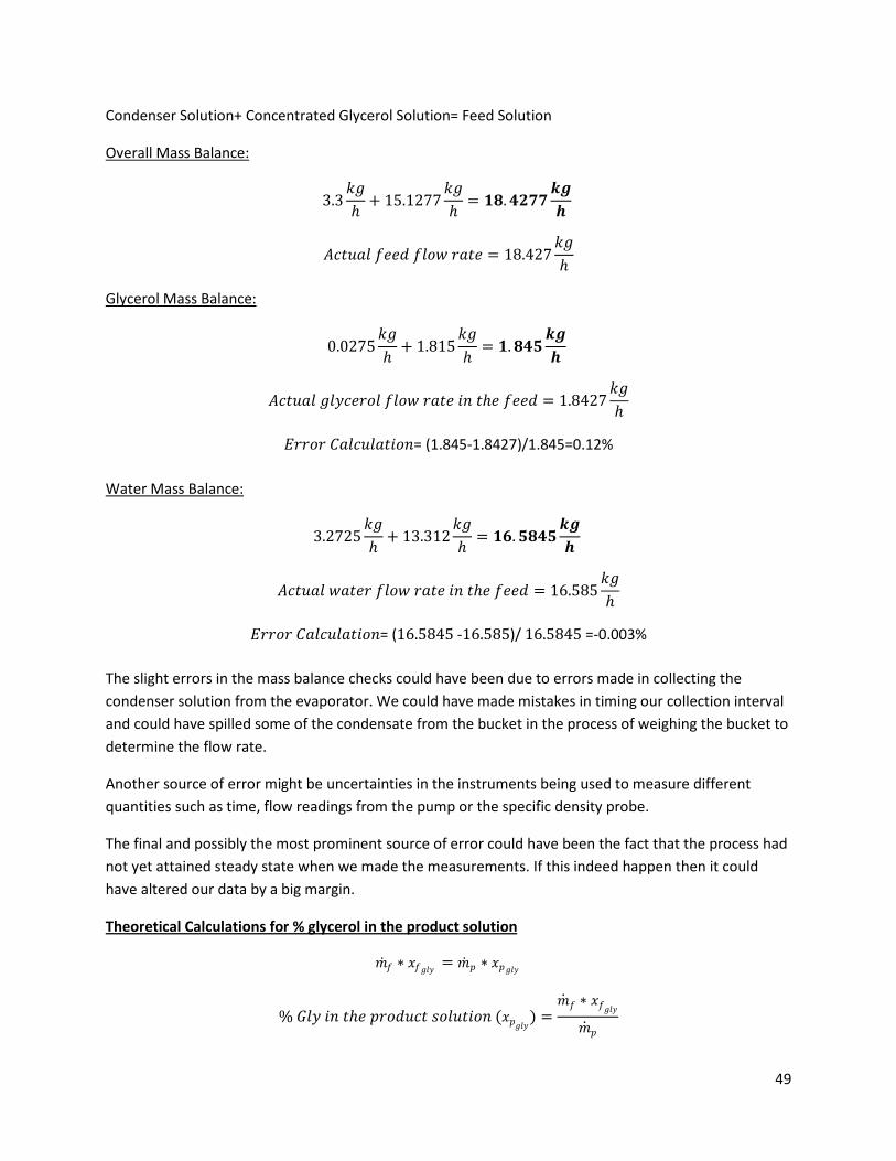
49

Condenser Solution+ Concentrated Glycerol Solution= Feed Solution

Overall Mass Balance:

3.3𝑘𝑘𝑔𝑔ℎ

+ 15.1277𝑘𝑘𝑔𝑔ℎ

= 𝟏𝟏𝟏𝟏.𝟒𝟒𝟎𝟎𝟎𝟎𝟎𝟎𝒌𝒌𝒌𝒌𝒉𝒉

𝐴𝐴𝑐𝑐𝑑𝑑𝑠𝑠𝐴𝐴𝐺𝐺 𝑓𝑓𝑓𝑓𝑓𝑓𝑓𝑓 𝑓𝑓𝐺𝐺𝑜𝑜𝑤𝑤 𝐴𝐴𝐴𝐴𝑑𝑑𝑓𝑓 = 18.427𝑘𝑘𝑔𝑔ℎ

Glycerol Mass Balance:

0.0275𝑘𝑘𝑔𝑔ℎ

+ 1.815𝑘𝑘𝑔𝑔ℎ

= 𝟏𝟏.𝟏𝟏𝟒𝟒𝟖𝟖𝒌𝒌𝒌𝒌𝒉𝒉

𝐴𝐴𝑐𝑐𝑑𝑑𝑠𝑠𝐴𝐴𝐺𝐺 𝑔𝑔𝐺𝐺𝐺𝐺𝑐𝑐𝑓𝑓𝐴𝐴𝑜𝑜𝐺𝐺 𝑓𝑓𝐺𝐺𝑜𝑜𝑤𝑤 𝐴𝐴𝐴𝐴𝑑𝑑𝑓𝑓 𝑑𝑑𝑑𝑑 𝑑𝑑ℎ𝑓𝑓 𝑓𝑓𝑓𝑓𝑓𝑓𝑓𝑓 = 1.8427𝑘𝑘𝑔𝑔ℎ

𝐸𝐸𝐴𝐴𝐴𝐴𝑜𝑜𝐴𝐴 𝐶𝐶𝐴𝐴𝐺𝐺𝑐𝑐𝑠𝑠𝐺𝐺𝐴𝐴𝑑𝑑𝑑𝑑𝑜𝑜𝑑𝑑= (1.845-1.8427)/1.845=0.12%

Water Mass Balance:

3.2725𝑘𝑘𝑔𝑔ℎ

+ 13.312𝑘𝑘𝑔𝑔ℎ

= 𝟏𝟏𝟎𝟎.𝟖𝟖𝟏𝟏𝟒𝟒𝟖𝟖𝒌𝒌𝒌𝒌𝒉𝒉

𝐴𝐴𝑐𝑐𝑑𝑑𝑠𝑠𝐴𝐴𝐺𝐺 𝑤𝑤𝐴𝐴𝑑𝑑𝑓𝑓𝐴𝐴 𝑓𝑓𝐺𝐺𝑜𝑜𝑤𝑤 𝐴𝐴𝐴𝐴𝑑𝑑𝑓𝑓 𝑑𝑑𝑑𝑑 𝑑𝑑ℎ𝑓𝑓 𝑓𝑓𝑓𝑓𝑓𝑓𝑓𝑓 = 16.585𝑘𝑘𝑔𝑔ℎ

𝐸𝐸𝐴𝐴𝐴𝐴𝑜𝑜𝐴𝐴 𝐶𝐶𝐴𝐴𝐺𝐺𝑐𝑐𝑠𝑠𝐺𝐺𝐴𝐴𝑑𝑑𝑑𝑑𝑜𝑜𝑑𝑑= (16.5845 -16.585)/ 16.5845 =-0.003%

The slight errors in the mass balance checks could have been due to errors made in collecting the condenser solution from the evaporator. We could have made mistakes in timing our collection interval and could have spilled some of the condensate from the bucket in the process of weighing the bucket to determine the flow rate.

Another source of error might be uncertainties in the instruments being used to measure different quantities such as time, flow readings from the pump or the specific density probe.

The final and possibly the most prominent source of error could have been the fact that the process had not yet attained steady state when we made the measurements. If this indeed happen then it could have altered our data by a big margin.

Theoretical Calculations for % glycerol in the product solution

�̇�𝑐𝑓𝑓 ∗ 𝑥𝑥𝑓𝑓𝑔𝑔𝐺𝐺𝐺𝐺 = �̇�𝑐𝑝𝑝 ∗ 𝑥𝑥𝑝𝑝𝑔𝑔𝐺𝐺𝐺𝐺

% 𝐺𝐺𝐺𝐺𝐺𝐺 𝑑𝑑𝑑𝑑 𝑑𝑑ℎ𝑓𝑓 𝑝𝑝𝐴𝐴𝑜𝑜𝑓𝑓𝑠𝑠𝑐𝑐𝑑𝑑 𝑑𝑑𝑜𝑜𝐺𝐺𝑠𝑠𝑑𝑑𝑑𝑑𝑜𝑜𝑑𝑑 (𝑥𝑥𝑝𝑝𝑔𝑔𝐺𝐺𝐺𝐺) =�̇�𝑐𝑓𝑓 ∗ 𝑥𝑥𝑓𝑓𝑔𝑔𝐺𝐺𝐺𝐺

�̇�𝑐𝑝𝑝

50

% 𝐺𝐺𝐺𝐺𝐺𝐺 𝑑𝑑𝑑𝑑 𝑑𝑑ℎ𝑓𝑓 𝑝𝑝𝐴𝐴𝑜𝑜𝑓𝑓𝑠𝑠𝑐𝑐𝑑𝑑 𝑑𝑑𝑜𝑜𝐺𝐺𝑠𝑠𝑑𝑑𝑑𝑑𝑜𝑜𝑑𝑑 �𝑥𝑥𝑝𝑝𝑔𝑔𝐺𝐺𝐺𝐺� =18.427 ∗ 0.1

15.1277= 12.2%

The theoretical % of glycerol in the product solution is slightly higher than the % glycerol actually measured in the product solution. This slight discrepancy can be attributed to experimental error. We might have made mistakes in cooling down the product solution to 25oC *(we might have over or under cooled) which might have given us faulty readings. We also could have made a mistake in reading off the % of glycerol from the percentage-specific gravity charts.

Sample Calculations for Energy Balance

Heat Flow from Steam to Water (Q)

𝑄𝑄𝑆𝑆 = �̇�𝑐𝑑𝑑𝜆𝜆𝑑𝑑

𝑄𝑄𝑆𝑆 = 𝑄𝑄𝑝𝑝 + 𝑄𝑄𝐸𝐸

𝑄𝑄𝑆𝑆 = �̇�𝑐𝐴𝐴𝜆𝜆 + �̇�𝑐𝑓𝑓𝐶𝐶𝑝𝑝𝛥𝛥𝛥𝛥 + 𝑄𝑄𝐸𝐸

Where: 𝑄𝑄𝐸𝐸 = 𝐸𝐸𝑑𝑑𝑓𝑓𝐴𝐴𝑔𝑔𝐺𝐺 𝐺𝐺𝑜𝑜𝑑𝑑𝑑𝑑𝑓𝑓𝑑𝑑 𝑑𝑑𝑜𝑜 𝑑𝑑ℎ𝑓𝑓 𝑓𝑓𝑑𝑑𝐴𝐴𝑑𝑑𝐴𝐴𝑜𝑜𝑑𝑑𝑐𝑐𝑓𝑓𝑑𝑑𝑑𝑑 �̇�𝑐𝐴𝐴𝐹𝐹𝐺𝐺𝑜𝑜𝑤𝑤 𝐴𝐴𝐴𝐴𝑑𝑑𝑓𝑓 𝑜𝑜𝑓𝑓 𝑑𝑑ℎ𝑓𝑓 𝑐𝑐𝑜𝑜𝑑𝑑𝑓𝑓𝑓𝑓𝑑𝑑𝑑𝑑𝑓𝑓𝐴𝐴 𝑑𝑑𝑜𝑜𝐺𝐺𝑠𝑠𝑑𝑑𝑑𝑑𝑜𝑜𝑑𝑑 𝜆𝜆 = 𝐿𝐿𝐴𝐴𝑑𝑑𝑓𝑓𝑑𝑑𝑑𝑑 𝐻𝐻𝑓𝑓𝐴𝐴𝑑𝑑 𝐶𝐶𝐴𝐴𝑝𝑝𝐴𝐴𝑐𝑐𝑑𝑑𝑑𝑑𝐺𝐺 𝑜𝑜𝑓𝑓 𝑑𝑑ℎ𝑓𝑓 𝑑𝑑𝑜𝑜𝐺𝐺𝑠𝑠𝑑𝑑𝑑𝑑𝑜𝑜𝑑𝑑 �̇�𝑐𝑓𝑓 = 𝑀𝑀𝐴𝐴𝑑𝑑𝑑𝑑 𝑓𝑓𝐺𝐺𝑜𝑜𝑤𝑤 𝐴𝐴𝐴𝐴𝑑𝑑𝑓𝑓 𝑜𝑜𝑓𝑓 𝑑𝑑ℎ𝑓𝑓 𝑓𝑓𝑓𝑓𝑓𝑓𝑓𝑓 𝑑𝑑𝑜𝑜𝐺𝐺𝑠𝑠𝑑𝑑𝑑𝑑𝑜𝑜𝑑𝑑 𝐶𝐶𝑝𝑝 = 𝑆𝑆𝑝𝑝𝑓𝑓𝑐𝑐𝑑𝑑𝑓𝑓𝑑𝑑𝑐𝑐 𝐻𝐻𝑓𝑓𝐴𝐴𝑑𝑑 𝐶𝐶𝐴𝐴𝑝𝑝𝐴𝐴𝑐𝑐𝑑𝑑𝑑𝑑𝐺𝐺 𝑜𝑜𝑓𝑓 𝑑𝑑ℎ𝑓𝑓 𝑓𝑓𝑓𝑓𝑓𝑓𝑓𝑓 𝑑𝑑𝑜𝑜𝐺𝐺𝑠𝑠𝑑𝑑𝑑𝑑𝑜𝑜𝑑𝑑 𝛥𝛥𝛥𝛥 = �𝛥𝛥𝑏𝑏𝑜𝑜𝑑𝑑𝐺𝐺𝑑𝑑𝑑𝑑𝑔𝑔 −𝛥𝛥𝑓𝑓𝑓𝑓𝑓𝑓𝑓𝑓 � The heat flowing from the steam to the feed solution (𝑄𝑄𝑃𝑃 heat gained by the process) is expressed in watts and calculated from an energy balance on the feed and the outgoing streams which are:

• Product( saturated hot liquid phase liquid leaving the evaporator) • Condensate ( saturated vapor leaving the evaporator, then being condensed and cooled)

To calculate the energy balance we first need to calculate the latent heat for the solution which comes out of the condenser.(Cite paper here). Latent heat calculations for solution with water as a solvent are not as straightforward as taking an average of the latent heat capacities of the components of the solution. From a paper we are going to us 1600 kj/kg as the heat capacity of the feed solution. We first need to calculate the percentage of water and glycerol in the solution. The calculations are given below:

𝐿𝐿𝐴𝐴𝑑𝑑𝑓𝑓𝑑𝑑𝑑𝑑 𝐻𝐻𝑓𝑓𝐴𝐴𝑑𝑑 𝑜𝑜𝑓𝑓 𝑑𝑑ℎ𝑓𝑓 𝑑𝑑𝑜𝑜𝐺𝐺𝑠𝑠𝑑𝑑𝑑𝑑𝑜𝑜𝑑𝑑 (𝜆𝜆𝑑𝑑𝑜𝑜𝐺𝐺𝑑𝑑 ) = 𝟏𝟏𝟎𝟎𝟎𝟎𝟎𝟎𝑘𝑘𝑘𝑘𝑘𝑘𝑔𝑔

Converting the latent heat of the solution from kJ/kg to J/kg

𝐿𝐿𝐴𝐴𝑑𝑑𝑓𝑓𝑑𝑑𝑑𝑑 𝐻𝐻𝑓𝑓𝐴𝐴𝑑𝑑 𝑜𝑜𝑓𝑓 𝑑𝑑ℎ𝑓𝑓 𝑑𝑑𝑜𝑜𝐺𝐺𝑠𝑠𝑑𝑑𝑑𝑑𝑜𝑜𝑑𝑑 (𝜆𝜆𝑑𝑑𝑜𝑜𝐺𝐺𝑑𝑑 ) = 𝟏𝟏𝟎𝟎𝟎𝟎𝟎𝟎𝟎𝟎𝟎𝟎𝟎𝟎𝑘𝑘𝑘𝑘𝑔𝑔

51

Step 2: Calculating the specific heat capacity of the concentrated glycerol solution:

𝑀𝑀𝐴𝐴𝑑𝑑𝑑𝑑 𝑓𝑓𝐺𝐺𝑜𝑜𝑤𝑤 𝐴𝐴𝐴𝐴𝑑𝑑𝑓𝑓 𝑜𝑜𝑓𝑓 𝑑𝑑ℎ𝑓𝑓 𝑓𝑓𝑓𝑓𝑓𝑓𝑓𝑓 𝑑𝑑𝑜𝑜𝐺𝐺𝑠𝑠𝑑𝑑𝑑𝑑𝑜𝑜𝑑𝑑 ��̇�𝑐𝑓𝑓� = 18.427 𝑘𝑘𝑔𝑔ℎ

% 𝑜𝑜𝑓𝑓 𝐺𝐺𝐺𝐺𝐺𝐺𝑐𝑐𝑓𝑓𝐴𝐴𝑜𝑜𝐺𝐺 𝑑𝑑𝑑𝑑 𝑑𝑑ℎ𝑓𝑓 𝑓𝑓𝑓𝑓𝑓𝑓𝑓𝑓 𝑑𝑑𝑜𝑜𝐺𝐺𝑠𝑠𝑑𝑑𝑑𝑑𝑜𝑜𝑑𝑑 �𝑥𝑥𝑓𝑓𝑔𝑔𝐺𝐺𝐺𝐺� = 10% = 0.10

𝑆𝑆𝑝𝑝𝑓𝑓𝑐𝑐𝑑𝑑𝑓𝑓𝑑𝑑𝑐𝑐 𝐻𝐻𝑓𝑓𝐴𝐴𝑑𝑑 𝐶𝐶𝐴𝐴𝑝𝑝𝐴𝐴𝑐𝑐𝑑𝑑𝑑𝑑𝐺𝐺 𝑜𝑜𝑓𝑓 𝑔𝑔𝐺𝐺𝐺𝐺𝑐𝑐𝑓𝑓𝐴𝐴𝑜𝑜𝐺𝐺 = 221.9𝑘𝑘

𝑐𝑐𝑜𝑜𝐺𝐺 ∗ 𝐾𝐾

Converting the specific heat capacity of glycerol from J/mol.K to J/kg.K

𝑀𝑀𝑜𝑜𝐺𝐺𝑓𝑓𝑐𝑐𝑠𝑠𝐺𝐺𝐴𝐴𝐴𝐴 𝑀𝑀𝐴𝐴𝑑𝑑𝑑𝑑 𝑜𝑜𝑓𝑓 𝐺𝐺𝐺𝐺𝐺𝐺𝑐𝑐𝑓𝑓𝐴𝐴𝑜𝑜𝐺𝐺 = 92.09 𝑔𝑔𝑐𝑐𝑜𝑜𝐺𝐺

𝑆𝑆𝑝𝑝𝑓𝑓𝑐𝑐𝑑𝑑𝑓𝑓𝑑𝑑𝑐𝑐 𝐻𝐻𝑓𝑓𝐴𝐴𝑑𝑑 𝐶𝐶𝐴𝐴𝑝𝑝𝐴𝐴𝑐𝑐𝑑𝑑𝑑𝑑𝐺𝐺 𝑜𝑜𝑓𝑓 𝑔𝑔𝐺𝐺𝐺𝐺𝑐𝑐𝑓𝑓𝐴𝐴𝑜𝑜𝐺𝐺 =221.992.09

𝑘𝑘

𝑔𝑔𝑐𝑐 ∗ 𝐾𝐾

𝑆𝑆𝑝𝑝𝑓𝑓𝑐𝑐𝑑𝑑𝑓𝑓𝑑𝑑𝑐𝑐 𝐻𝐻𝑓𝑓𝐴𝐴𝑑𝑑 𝐶𝐶𝐴𝐴𝑝𝑝𝐴𝐴𝑐𝑐𝑑𝑑𝑑𝑑𝐺𝐺 𝑜𝑜𝑓𝑓 𝑔𝑔𝐺𝐺𝐺𝐺𝑐𝑐𝑓𝑓𝐴𝐴𝑜𝑜𝐺𝐺 = 2.409 𝑘𝑘

𝑔𝑔𝑐𝑐 ∗ 𝐾𝐾

𝑆𝑆𝑝𝑝𝑓𝑓𝑐𝑐𝑑𝑑𝑓𝑓𝑑𝑑𝑐𝑐 𝐻𝐻𝑓𝑓𝐴𝐴𝑑𝑑 𝐶𝐶𝐴𝐴𝑝𝑝𝐴𝐴𝑐𝑐𝑑𝑑𝑑𝑑𝐺𝐺 𝑜𝑜𝑓𝑓 𝑔𝑔𝐺𝐺𝐺𝐺𝑐𝑐𝑓𝑓𝐴𝐴𝑜𝑜𝐺𝐺 = 2.409 ∗ 1000 𝑘𝑘

𝑘𝑘𝑔𝑔 ∗ 𝐾𝐾

𝑆𝑆𝑝𝑝𝑓𝑓𝑐𝑐𝑑𝑑𝑓𝑓𝑑𝑑𝑐𝑐 𝐻𝐻𝑓𝑓𝐴𝐴𝑑𝑑 𝐶𝐶𝐴𝐴𝑝𝑝𝐴𝐴𝑐𝑐𝑑𝑑𝑑𝑑𝐺𝐺 𝑜𝑜𝑓𝑓 𝑔𝑔𝐺𝐺𝐺𝐺𝑐𝑐𝑓𝑓𝐴𝐴𝑜𝑜𝐺𝐺 = 2409.499 𝑘𝑘

𝑘𝑘𝑔𝑔 ∗ 𝐾𝐾

% 𝑜𝑜𝑓𝑓𝑤𝑤𝐴𝐴𝑑𝑑𝑓𝑓𝐴𝐴 𝑑𝑑𝑑𝑑 𝑑𝑑ℎ𝑓𝑓 𝑓𝑓𝑓𝑓𝑓𝑓𝑓𝑓 𝑑𝑑𝑜𝑜𝐺𝐺𝑠𝑠𝑑𝑑𝑑𝑑𝑜𝑜𝑑𝑑 �𝑥𝑥𝑓𝑓𝑔𝑔𝐺𝐺𝐺𝐺� = 90% = 0.90

𝑆𝑆𝑝𝑝𝑓𝑓𝑐𝑐𝑑𝑑𝑓𝑓𝑑𝑑𝑐𝑐 𝐻𝐻𝑓𝑓𝐴𝐴𝑑𝑑 𝐶𝐶𝐴𝐴𝑝𝑝𝐴𝐴𝑐𝑐𝑑𝑑𝑑𝑑𝐺𝐺 𝑜𝑜𝑓𝑓 𝑤𝑤𝐴𝐴𝑑𝑑𝑓𝑓𝐴𝐴 = 4186 𝑘𝑘

𝑘𝑘𝑔𝑔 ∗ 𝐾𝐾

𝑆𝑆𝑝𝑝𝑓𝑓𝑐𝑐𝑑𝑑𝑓𝑓𝑑𝑑𝑐𝑐 𝐻𝐻𝑓𝑓𝐴𝐴𝑑𝑑 𝐶𝐶𝐴𝐴𝑝𝑝𝐴𝐴𝑐𝑐𝑑𝑑𝑑𝑑𝐺𝐺 𝑜𝑜𝑓𝑓 𝑝𝑝𝐴𝐴𝑜𝑜𝑓𝑓𝑠𝑠𝑐𝑐𝑑𝑑 𝑑𝑑𝑜𝑜𝐺𝐺𝑠𝑠𝑑𝑑𝑑𝑑𝑜𝑜𝑑𝑑 = �0.90 ∗ 4186 𝑘𝑘

𝑘𝑘𝑔𝑔 ∗ 𝐾𝐾� + �0.10 ∗ 2409.499

𝑘𝑘𝑘𝑘𝑔𝑔 ∗ 𝐾𝐾

�

𝑆𝑆𝑝𝑝𝑓𝑓𝑐𝑐𝑑𝑑𝑓𝑓𝑑𝑑𝑐𝑐 𝐻𝐻𝑓𝑓𝐴𝐴𝑑𝑑 𝐶𝐶𝐴𝐴𝑝𝑝𝐴𝐴𝑐𝑐𝑑𝑑𝑑𝑑𝐺𝐺 𝑜𝑜𝑓𝑓 𝑑𝑑ℎ𝑓𝑓 𝑓𝑓𝑓𝑓𝑓𝑓𝑓𝑓 𝑑𝑑𝑜𝑜𝐺𝐺𝑠𝑠𝑑𝑑𝑑𝑑𝑜𝑜𝑑𝑑(𝐶𝐶𝑝𝑝𝑓𝑓) = 𝟒𝟒𝟎𝟎𝟎𝟎𝟏𝟏.𝟎𝟎𝟖𝟖𝑱𝑱

𝒌𝒌𝒌𝒌 ∗ 𝑲𝑲

Step 3: Calculating the temperature difference

𝐵𝐵𝑜𝑜𝑑𝑑𝐺𝐺𝑑𝑑𝑑𝑑𝑔𝑔 𝑑𝑑𝑓𝑓𝑐𝑐𝑝𝑝𝑓𝑓𝐴𝐴𝐴𝐴𝑑𝑑𝑠𝑠𝐴𝐴𝑓𝑓 𝑓𝑓𝑜𝑜𝐴𝐴 𝑑𝑑ℎ𝑓𝑓 𝑓𝑓𝑓𝑓𝑓𝑓𝑓𝑓 𝑑𝑑𝑜𝑜𝐺𝐺𝑠𝑠𝑑𝑑𝑑𝑑𝑜𝑜𝑑𝑑(𝛥𝛥𝑏𝑏) = 376.15 𝐾𝐾

𝐼𝐼𝑑𝑑𝐺𝐺𝑓𝑓𝑑𝑑 𝑑𝑑𝑓𝑓𝑐𝑐𝑝𝑝𝑓𝑓𝐴𝐴𝐴𝐴𝑑𝑑𝑠𝑠𝐴𝐴𝑓𝑓 𝑓𝑓𝑜𝑜𝐴𝐴 𝑑𝑑ℎ𝑓𝑓 𝑓𝑓𝑓𝑓𝑓𝑓𝑓𝑓 𝑑𝑑𝑜𝑜𝐺𝐺𝑠𝑠𝑑𝑑𝑑𝑑𝑜𝑜𝑑𝑑�𝛥𝛥𝑓𝑓� = 84 𝐹𝐹

𝑑𝑑𝐺𝐺𝑓𝑓𝑑𝑑 𝑑𝑑𝑓𝑓𝑐𝑐𝑝𝑝𝑓𝑓𝐴𝐴𝐴𝐴𝑑𝑑𝑠𝑠𝐴𝐴𝑓𝑓 𝑓𝑓𝑜𝑜𝐴𝐴 𝑑𝑑ℎ𝑓𝑓 𝑓𝑓𝑓𝑓𝑓𝑓𝑓𝑓 𝑑𝑑𝑜𝑜𝐺𝐺𝑠𝑠𝑑𝑑𝑑𝑑𝑜𝑜𝑑𝑑�𝛥𝛥𝑓𝑓� = 302.04 𝐾𝐾

𝛥𝛥𝑓𝑓𝑐𝑐𝑝𝑝𝑓𝑓𝐴𝐴𝐴𝐴𝑑𝑑𝑠𝑠𝐴𝐴𝑓𝑓 𝑓𝑓𝑑𝑑𝑓𝑓𝑓𝑓𝑓𝑓𝐴𝐴𝑓𝑓𝑑𝑑𝑐𝑐𝑓𝑓 �𝛥𝛥𝑏𝑏 − 𝛥𝛥𝑓𝑓� = 373.15 𝐾𝐾 − 302.04 𝐾𝐾 = 71.94𝐾𝐾

Step 4: Calculating the heat gained by the process:

52

𝑄𝑄𝑝𝑝 = [�̇�𝑐𝑓𝑓𝐶𝐶𝑝𝑝𝑓𝑓 ∗ �𝛥𝛥𝑏𝑏 − 𝛥𝛥𝑓𝑓�] + [�̇�𝑐𝐴𝐴𝜆𝜆𝑓𝑓]

𝑄𝑄𝑝𝑝 = (18.427𝑘𝑘𝑔𝑔ℎ∗ 4008.35

𝑘𝑘𝑘𝑘𝑔𝑔 ∗ 𝐾𝐾

∗ (71.94𝐾𝐾) + �3.3𝑘𝑘𝑔𝑔ℎ∗ 1600000

𝑘𝑘𝑘𝑘𝑔𝑔�

𝑄𝑄𝑝𝑝 = 10754015 𝑘𝑘ℎ

Converting this from Joules/ hour to Watts:

𝑄𝑄𝑝𝑝 =10754015 𝑘𝑘ℎ

3600 𝑑𝑑𝑓𝑓𝑐𝑐ℎ= 2987.251 𝑊𝑊𝐴𝐴𝑑𝑑𝑑𝑑𝑑𝑑

𝑄𝑄𝑝𝑝 = 𝟎𝟎.𝟗𝟗𝟏𝟏𝟎𝟎𝟎𝟎 𝒌𝒌𝒌𝒌

Step 5: Calculating the heat lost by the steam:

𝑄𝑄𝑆𝑆 = �̇�𝑐𝑑𝑑𝜆𝜆𝑑𝑑

Where:

�̇�𝑐𝑑𝑑 is the condensate mass flow rate

𝜆𝜆𝑑𝑑 is the latent heat of vaporization for steam

𝐶𝐶𝑜𝑜𝑑𝑑𝑓𝑓𝑓𝑓𝑑𝑑𝑑𝑑𝐴𝐴𝑑𝑑𝑓𝑓 𝑀𝑀𝐴𝐴𝑑𝑑𝑑𝑑 𝐹𝐹𝐺𝐺𝑜𝑜𝑤𝑤 𝑅𝑅𝐴𝐴𝑑𝑑𝑓𝑓 (�̇�𝑐𝑑𝑑) = 9.6𝑘𝑘𝑔𝑔ℎ

𝐶𝐶𝑜𝑜𝑑𝑑𝑓𝑓𝑓𝑓𝑑𝑑𝑑𝑑𝐴𝐴𝑑𝑑𝑓𝑓 𝑀𝑀𝐴𝐴𝑑𝑑𝑑𝑑 𝐹𝐹𝐺𝐺𝑜𝑜𝑤𝑤 𝑅𝑅𝐴𝐴𝑑𝑑𝑓𝑓 (�̇�𝑐𝑑𝑑) = 0.002667𝑘𝑘𝑔𝑔𝑑𝑑𝑓𝑓𝑐𝑐

𝑄𝑄𝑆𝑆 = 0.002667𝑘𝑘𝑔𝑔𝑑𝑑𝑓𝑓𝑐𝑐

∗ 2769000𝑘𝑘𝑘𝑘𝑔𝑔

𝑄𝑄𝑆𝑆 = 7384 𝑊𝑊𝐴𝐴𝑑𝑑𝑑𝑑𝑑𝑑

Calculating the heat lost to the environment using the overall energy balance for the evaporator:

𝑄𝑄𝑆𝑆 = 𝑄𝑄𝑝𝑝 + 𝑄𝑄𝐸𝐸

𝑄𝑄𝐸𝐸 = 𝑄𝑄𝑆𝑆 − 𝑄𝑄𝑝𝑝

𝑄𝑄𝐸𝐸 = 7384 𝑊𝑊− 2987.251𝑊𝑊 = 4396.75 𝑊𝑊𝐴𝐴𝑑𝑑𝑑𝑑𝑑𝑑

Q to boil

Q to evaporate

53

𝑄𝑄𝐸𝐸 = 4.396 𝑘𝑘𝑊𝑊

Step 1: Calculating the quality of the steam

𝐸𝐸𝑑𝑑𝑑𝑑ℎ𝐴𝐴𝐺𝐺𝑝𝑝𝐺𝐺 𝑜𝑜𝑓𝑓 𝑆𝑆𝑠𝑠𝑝𝑝𝑓𝑓𝐴𝐴ℎ𝑓𝑓𝐴𝐴𝑑𝑑𝑓𝑓𝑓𝑓 𝑆𝑆𝑑𝑑𝑓𝑓𝐴𝐴𝑐𝑐 �𝐻𝐻𝑑𝑑𝑠𝑠𝑝𝑝𝑓𝑓𝐴𝐴 � = 1157.42

𝐸𝐸𝑑𝑑𝑑𝑑ℎ𝐴𝐴𝐺𝐺𝑝𝑝𝐺𝐺 𝑜𝑜𝑓𝑓 𝑆𝑆𝐴𝐴𝑑𝑑𝑠𝑠𝐴𝐴𝐴𝐴𝑑𝑑𝑓𝑓𝑓𝑓 𝑆𝑆𝑑𝑑𝑓𝑓𝐴𝐴𝑐𝑐 (𝐻𝐻𝑑𝑑𝐴𝐴𝑑𝑑 ) = 1150.5

𝐸𝐸𝑑𝑑𝑑𝑑ℎ𝐴𝐴𝐺𝐺𝑝𝑝𝐺𝐺 𝑜𝑜𝑓𝑓 𝑑𝑑ℎ𝑓𝑓 𝑐𝑐𝑜𝑜𝑑𝑑𝑓𝑓𝑓𝑓𝑑𝑑𝑑𝑑𝐴𝐴𝑑𝑑𝑓𝑓 (𝐻𝐻𝑐𝑐𝑜𝑜𝑑𝑑𝑓𝑓 ) = 180.16

𝑄𝑄𝑠𝑠𝐴𝐴𝐺𝐺𝑑𝑑𝑑𝑑𝐺𝐺 𝑜𝑜𝑓𝑓𝑓𝑓 𝑆𝑆𝑑𝑑𝑓𝑓𝐴𝐴𝑐𝑐 (𝑋𝑋) =𝐻𝐻𝑐𝑐𝑜𝑜𝑑𝑑𝑓𝑓 − 𝐻𝐻𝑑𝑑𝑠𝑠𝑝𝑝𝑓𝑓𝐴𝐴𝐻𝐻𝑐𝑐𝑜𝑜𝑑𝑑𝑓𝑓 − 𝐻𝐻𝑑𝑑𝐴𝐴𝑑𝑑

𝑄𝑄𝑠𝑠𝐴𝐴𝐺𝐺𝑑𝑑𝑑𝑑𝐺𝐺 𝑜𝑜𝑓𝑓𝑓𝑓 𝑆𝑆𝑑𝑑𝑓𝑓𝐴𝐴𝑐𝑐 (𝑋𝑋) =180.16− 1157.42180.16− 1150.5

= 1.000334

Table of heat loss and gain values at two different operating pressures:

Sample Calculations for Heat Transfer Coefficients

1𝑈𝑈𝐴𝐴

=1

ℎ𝑑𝑑 ∗ 𝐴𝐴𝑑𝑑+

𝑞𝑞𝑘𝑘𝑞𝑞 ∗ 𝐴𝐴

+1

ℎ𝑜𝑜 ∗ 𝐴𝐴𝑜𝑜

For the process of concentrating glycerol using the climbing film evaporator there is an outer overall heat transfer coefficient which is given by the expression:

𝑄𝑄𝐸𝐸 = 𝑈𝑈𝑂𝑂𝐸𝐸 ∗ 𝐴𝐴𝑂𝑂 ∗ ∆𝛥𝛥𝐿𝐿𝑀𝑀

Where:

𝑈𝑈𝑂𝑂𝐸𝐸 is the outer heat transfer coefficient

𝐴𝐴𝑂𝑂 is the outer surface area of the evaporator

Pressure(psig) Feed Flow Rate (kg/h) Q gained by the process (QP)

Q loss to the environment (QE)

5 7.3710 2.0659 3.7011 5 12.285 2.1977 4.0325 5 18.427 2.5689 4.3531 5 24.570 2.8030 4.3501 10 7.3710 2.47947 3.52 10 12.285 2.75088 4.1716 10 18.427 2.98725 4.3967 10 24.570 3.2275 4.3873

54

∆𝛥𝛥𝐿𝐿𝑀𝑀 is the Log mean temperature difference or the driving force with steam on the inside and air outside( which in this case is just (𝛥𝛥𝑑𝑑 − 𝛥𝛥𝐴𝐴)

Since we already calculated the energy lost to the environment we can rearrange the equation to

𝑈𝑈𝑂𝑂𝐸𝐸 =𝑄𝑄𝐸𝐸

𝐴𝐴𝑂𝑂 ∗ (𝛥𝛥𝑑𝑑 − 𝛥𝛥𝐴𝐴)

𝐻𝐻𝑓𝑓𝐴𝐴𝑑𝑑 𝑓𝑓𝑑𝑑𝑓𝑓𝐴𝐴𝑔𝑔𝐺𝐺 𝐺𝐺𝑜𝑜𝑑𝑑 𝑑𝑑𝑜𝑜 𝑑𝑑ℎ𝑓𝑓 𝑓𝑓𝑑𝑑𝐴𝐴𝑑𝑑𝐴𝐴𝑜𝑜𝑑𝑑𝑐𝑐𝑓𝑓𝑑𝑑𝑑𝑑(𝑄𝑄𝐸𝐸) = 4396.75 𝑊𝑊𝐴𝐴𝑑𝑑𝑑𝑑𝑑𝑑

𝛥𝛥𝑓𝑓𝑐𝑐𝑝𝑝𝑓𝑓𝐴𝐴𝐴𝐴𝑑𝑑𝑠𝑠𝐴𝐴𝑓𝑓 𝑜𝑜𝑓𝑓 𝑑𝑑ℎ𝑓𝑓 𝑑𝑑𝑑𝑑𝑓𝑓𝐴𝐴𝑐𝑐 𝑑𝑑𝑠𝑠𝑝𝑝𝑝𝑝𝐺𝐺𝑑𝑑𝑓𝑓𝑓𝑓 𝐴𝐴𝑑𝑑 10 𝑝𝑝𝑑𝑑𝑑𝑑𝑔𝑔 (𝛥𝛥𝑑𝑑) = 388.15 𝐾𝐾

𝛥𝛥𝑓𝑓𝑐𝑐𝑝𝑝𝑓𝑓𝐴𝐴𝐴𝐴𝑑𝑑𝑠𝑠𝐴𝐴𝑓𝑓 𝑜𝑜𝑓𝑓 𝑑𝑑ℎ𝑓𝑓 𝐴𝐴𝑑𝑑𝐴𝐴 𝑜𝑜𝑠𝑠𝑑𝑑𝑑𝑑𝑑𝑑𝑑𝑑𝑓𝑓𝑓𝑓 𝑑𝑑ℎ𝑓𝑓 𝑓𝑓𝐴𝐴𝐴𝐴𝑝𝑝𝑜𝑜𝐴𝐴𝐴𝐴𝑑𝑑𝑜𝑜𝐴𝐴 (𝛥𝛥𝐴𝐴) = 298.15 𝐾𝐾

𝛥𝛥𝑓𝑓𝑐𝑐𝑝𝑝𝑓𝑓𝐴𝐴𝐴𝐴𝑑𝑑𝑠𝑠𝐴𝐴𝑓𝑓 𝑓𝑓𝑑𝑑𝑓𝑓𝑓𝑓𝑓𝑓𝐴𝐴𝑓𝑓𝑑𝑑𝑐𝑐𝑓𝑓 (𝛥𝛥𝑑𝑑 − 𝛥𝛥𝐴𝐴) = 388.15 𝐾𝐾 − 298.15 𝐾𝐾 = 90 𝐾𝐾

Step 1: Calculating the outer surface area of the evaporator:

𝐷𝐷𝑑𝑑𝐴𝐴𝑐𝑐𝑓𝑓𝑑𝑑𝑓𝑓𝐴𝐴 𝑜𝑜𝑓𝑓 𝑑𝑑ℎ𝑓𝑓 𝑑𝑑𝑑𝑑𝑑𝑑𝑓𝑓𝐴𝐴 𝑑𝑑𝑠𝑠𝑏𝑏𝑓𝑓 ( 𝐷𝐷𝑑𝑑) = 1 𝑑𝑑𝑑𝑑

𝐷𝐷𝑑𝑑𝐴𝐴𝑐𝑐𝑓𝑓𝑑𝑑𝑓𝑓𝐴𝐴 𝑜𝑜𝑓𝑓 𝑑𝑑ℎ𝑓𝑓 𝑜𝑜𝑠𝑠𝑑𝑑𝑓𝑓𝐴𝐴 𝑑𝑑𝑠𝑠𝑏𝑏𝑓𝑓 ( 𝐷𝐷𝑜𝑜) = 2.5 𝑑𝑑𝑑𝑑

𝐷𝐷𝑑𝑑𝐴𝐴𝑐𝑐𝑓𝑓𝑑𝑑𝑓𝑓𝐴𝐴 𝑜𝑜𝑓𝑓 𝑑𝑑ℎ𝑓𝑓 𝑜𝑜𝑠𝑠𝑑𝑑𝑓𝑓𝐴𝐴 𝑑𝑑𝑠𝑠𝑏𝑏𝑓𝑓 ( 𝐷𝐷𝑜𝑜) =2.5 𝑑𝑑𝑑𝑑12 𝑑𝑑𝑑𝑑

∗ 𝑓𝑓𝑑𝑑 = 0.208 𝑓𝑓𝑑𝑑

𝐿𝐿𝑓𝑓𝑑𝑑𝑔𝑔ℎ𝑑𝑑 𝑜𝑜𝑓𝑓 𝑑𝑑ℎ𝑓𝑓 𝑓𝑓𝐴𝐴𝐴𝐴𝑝𝑝𝑜𝑜𝐴𝐴𝐴𝐴𝑑𝑑𝑜𝑜𝐴𝐴 (𝐿𝐿) = 9 𝑓𝑓𝑑𝑑

𝑂𝑂𝑠𝑠𝑑𝑑𝑓𝑓𝐴𝐴 𝐴𝐴𝐴𝐴𝑓𝑓𝐴𝐴 𝑜𝑜𝑓𝑓 𝑑𝑑ℎ𝑓𝑓 𝑓𝑓𝐴𝐴𝐴𝐴𝑝𝑝𝑜𝑜𝐴𝐴𝐴𝐴𝑑𝑑𝑜𝑜𝐴𝐴 (𝐴𝐴𝑂𝑂) =𝜋𝜋 ∗ 𝐷𝐷𝑜𝑜2 ∗ 𝐿𝐿

4

𝑂𝑂𝑠𝑠𝑑𝑑𝑓𝑓𝐴𝐴 𝐴𝐴𝐴𝐴𝑓𝑓𝐴𝐴 𝑜𝑜𝑓𝑓 𝑑𝑑ℎ𝑓𝑓 𝑓𝑓𝐴𝐴𝐴𝐴𝑝𝑝𝑜𝑜𝐴𝐴𝐴𝐴𝑑𝑑𝑜𝑜𝐴𝐴 (𝐴𝐴𝑂𝑂) = 0.306796 𝑓𝑓𝑑𝑑2

𝑂𝑂𝑠𝑠𝑑𝑑𝑓𝑓𝐴𝐴 𝐴𝐴𝐴𝐴𝑓𝑓𝐴𝐴 𝑜𝑜𝑓𝑓 𝑑𝑑ℎ𝑓𝑓 𝑓𝑓𝐴𝐴𝐴𝐴𝑝𝑝𝑜𝑜𝐴𝐴𝐴𝐴𝑑𝑑𝑜𝑜𝐴𝐴 (𝐴𝐴𝑂𝑂) = 0.028502 𝑐𝑐2

Step 1: Calculating the overall outer HT coefficient:

𝑈𝑈𝑂𝑂𝐸𝐸 =4396.75 𝑊𝑊𝐴𝐴𝑑𝑑𝑑𝑑𝑑𝑑

0.028502 𝑐𝑐2 ∗ 90 𝐾𝐾= 𝟏𝟏𝟎𝟎𝟏𝟏𝟒𝟒

𝒌𝒌𝒎𝒎𝟎𝟎 ∗ 𝑲𝑲

Calculating the inner heat transfer coefficient

In case of the evaporator process the inner heat transfer can be calculated in two ways:

• Consider the entire tube as a whole and neglect the phase change happening in the tube and consider the driving force to be between the feed inlet temperature and the outlet temperature

• Break down the tube into two processes

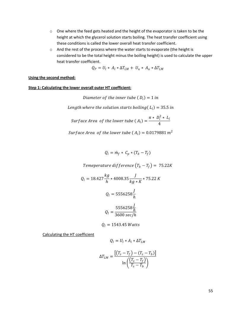
55

o One where the feed gets heated and the height of the evaporator is taken to be the height at which the glycerol solution starts boiling. The heat transfer coefficient using these conditions is called the lower overall heat transfer coefficient.

o And the rest of the process where the water starts to evaporate (the height is considered to be the total height minus the boiling height) is used to calculate the upper heat transfer coefficient.

𝑄𝑄𝑃𝑃 = 𝑈𝑈𝐺𝐺 ∗ 𝐴𝐴𝐺𝐺 ∗ ∆𝛥𝛥𝐿𝐿𝑀𝑀 + 𝑈𝑈𝑠𝑠 ∗ 𝐴𝐴𝑠𝑠 ∗ ∆𝛥𝛥𝐿𝐿𝑀𝑀

Using the second method:

Step 1: Calculating the lower overall outer HT coefficient:

𝐷𝐷𝑑𝑑𝐴𝐴𝑐𝑐𝑓𝑓𝑑𝑑𝑓𝑓𝐴𝐴 𝑜𝑜𝑓𝑓 𝑑𝑑ℎ𝑓𝑓 𝑑𝑑𝑑𝑑𝑑𝑑𝑓𝑓𝐴𝐴 𝑑𝑑𝑠𝑠𝑏𝑏𝑓𝑓 ( 𝐷𝐷𝑑𝑑) = 1 𝑑𝑑𝑑𝑑

𝐿𝐿𝑓𝑓𝑑𝑑𝑔𝑔𝑑𝑑ℎ 𝑤𝑤ℎ𝑓𝑓𝐴𝐴𝑓𝑓 𝑑𝑑ℎ𝑓𝑓 𝑑𝑑𝑜𝑜𝐺𝐺𝑠𝑠𝑑𝑑𝑑𝑑𝑜𝑜𝑑𝑑 𝑑𝑑𝑑𝑑𝐴𝐴𝐴𝐴𝑑𝑑𝑑𝑑 𝑏𝑏𝑜𝑜𝑑𝑑𝐺𝐺𝑑𝑑𝑑𝑑𝑔𝑔( 𝐿𝐿𝐺𝐺) = 35.5 𝑑𝑑𝑑𝑑

𝑆𝑆𝑠𝑠𝐴𝐴𝑓𝑓𝐴𝐴𝑐𝑐𝑓𝑓 𝐴𝐴𝐴𝐴𝑓𝑓𝐴𝐴 𝑜𝑜𝑓𝑓 𝑑𝑑ℎ𝑓𝑓 𝐺𝐺𝑜𝑜𝑤𝑤𝑓𝑓𝐴𝐴 𝑑𝑑𝑠𝑠𝑏𝑏𝑓𝑓 ( 𝐴𝐴𝐺𝐺) =𝜋𝜋 ∗ 𝐷𝐷𝑑𝑑2 ∗ 𝐿𝐿𝐺𝐺

4

𝑆𝑆𝑠𝑠𝐴𝐴𝑓𝑓𝐴𝐴𝑐𝑐𝑓𝑓 𝐴𝐴𝐴𝐴𝑓𝑓𝐴𝐴 𝑜𝑜𝑓𝑓 𝑑𝑑ℎ𝑓𝑓 𝐺𝐺𝑜𝑜𝑤𝑤𝑓𝑓𝐴𝐴 𝑑𝑑𝑠𝑠𝑏𝑏𝑓𝑓 ( 𝐴𝐴𝐺𝐺) = 0.0179881 𝑐𝑐2

𝑄𝑄𝐺𝐺 = �̇�𝑐𝑓𝑓 ∗ 𝐶𝐶𝑝𝑝 ∗ (𝛥𝛥𝑏𝑏 − 𝛥𝛥𝑓𝑓)

𝛥𝛥𝑓𝑓𝑐𝑐𝑓𝑓𝑝𝑝𝑓𝑓𝐴𝐴𝐴𝐴𝑑𝑑𝑠𝑠𝐴𝐴𝑓𝑓 𝑓𝑓𝑑𝑑𝑓𝑓𝑓𝑓𝑓𝑓𝐴𝐴𝑓𝑓𝑑𝑑𝑐𝑐𝑓𝑓 �𝛥𝛥𝑏𝑏 − 𝛥𝛥𝑓𝑓� = 75.22𝐾𝐾

𝑄𝑄𝐺𝐺 = 18.427𝑘𝑘𝑔𝑔ℎ∗ 4008.35

𝑘𝑘𝑘𝑘𝑔𝑔 ∗ 𝐾𝐾

∗ 75.22 𝐾𝐾

𝑄𝑄𝐺𝐺 = 5556258𝑘𝑘ℎ

𝑄𝑄𝐺𝐺 =5556258 𝑘𝑘ℎ3600 𝑑𝑑𝑓𝑓𝑐𝑐/ℎ

𝑄𝑄𝐺𝐺 = 1543.45 𝑊𝑊𝐴𝐴𝑑𝑑𝑑𝑑𝑑𝑑

Calculating the HT coefficient 𝑄𝑄𝐺𝐺 = 𝑈𝑈𝐺𝐺 ∗ 𝐴𝐴𝐺𝐺 ∗ ∆𝛥𝛥𝐿𝐿𝑀𝑀

∆𝛥𝛥𝐿𝐿𝑀𝑀 =��𝛥𝛥𝑑𝑑 − 𝛥𝛥𝑓𝑓� − (𝛥𝛥𝑑𝑑 − 𝛥𝛥𝑏𝑏)�

ln��𝛥𝛥𝑑𝑑 − 𝛥𝛥𝑓𝑓�𝛥𝛥𝑑𝑑 − 𝛥𝛥𝑏𝑏

�

56

∆𝛥𝛥𝐿𝐿𝑀𝑀 =[(388.15− 300.92)− (388.15− 376.15)]

ln �(388.15− 300.92)388.15− 376.15 �

∆𝑻𝑻𝑳𝑳𝑳𝑳 = 𝟎𝟎𝟏𝟏.𝟎𝟎 𝑲𝑲

𝑈𝑈𝐺𝐺 =𝑄𝑄𝐺𝐺

𝐴𝐴𝐺𝐺 ∗ ∆𝛥𝛥𝐿𝐿𝑀𝑀

𝑈𝑈𝐺𝐺 =1543.45 𝑊𝑊𝐴𝐴𝑑𝑑𝑑𝑑𝑑𝑑

0.0179881 𝑐𝑐2 ∗ 78.7 𝐾𝐾

𝑈𝑈𝐺𝐺 = 1090.21𝑊𝑊𝐴𝐴𝑑𝑑𝑑𝑑𝑑𝑑𝑐𝑐2 ∗ 𝐾𝐾

Step 2: Calculating the upper overall outer HT coefficient:

𝐷𝐷𝑑𝑑𝐴𝐴𝑐𝑐𝑓𝑓𝑑𝑑𝑓𝑓𝐴𝐴 𝑜𝑜𝑓𝑓 𝑑𝑑ℎ𝑓𝑓 𝑑𝑑𝑑𝑑𝑑𝑑𝑓𝑓𝐴𝐴 𝑑𝑑𝑠𝑠𝑏𝑏𝑓𝑓 ( 𝐷𝐷𝑑𝑑) = 1 𝑑𝑑𝑑𝑑

𝐿𝐿𝑓𝑓𝑑𝑑𝑔𝑔𝑑𝑑ℎ 𝑤𝑤ℎ𝑓𝑓𝐴𝐴𝑓𝑓 𝑑𝑑ℎ𝑓𝑓 𝑑𝑑𝑜𝑜𝐺𝐺𝑠𝑠𝑑𝑑𝑑𝑑𝑜𝑜𝑑𝑑 𝑑𝑑𝑑𝑑𝐴𝐴𝐴𝐴𝑑𝑑𝑑𝑑 𝑏𝑏𝑜𝑜𝑑𝑑𝐺𝐺𝑑𝑑𝑑𝑑𝑔𝑔( 𝐿𝐿𝐺𝐺) = 72.5 𝑑𝑑𝑑𝑑

𝑆𝑆𝑠𝑠𝐴𝐴𝑓𝑓𝐴𝐴𝑐𝑐𝑓𝑓 𝐴𝐴𝐴𝐴𝑓𝑓𝐴𝐴 𝑜𝑜𝑓𝑓 𝑑𝑑ℎ𝑓𝑓 𝐺𝐺𝑜𝑜𝑤𝑤𝑓𝑓𝐴𝐴 𝑑𝑑𝑠𝑠𝑏𝑏𝑓𝑓 ( 𝐴𝐴𝐺𝐺) =𝜋𝜋 ∗ 𝐷𝐷𝑑𝑑2 ∗ 𝐿𝐿𝐺𝐺

4

𝑆𝑆𝑠𝑠𝐴𝐴𝑓𝑓𝐴𝐴𝑐𝑐𝑓𝑓 𝐴𝐴𝐴𝐴𝑓𝑓𝐴𝐴 𝑜𝑜𝑓𝑓 𝑑𝑑ℎ𝑓𝑓 𝐺𝐺𝑜𝑜𝑤𝑤𝑓𝑓𝐴𝐴 𝑑𝑑𝑠𝑠𝑏𝑏𝑓𝑓 ( 𝐴𝐴𝐺𝐺) = 0.3673 𝑐𝑐2

𝑄𝑄𝑠𝑠 = �̇�𝑐𝐴𝐴 ∗ 𝜆𝜆

𝑄𝑄𝑠𝑠 = 3.3𝑘𝑘𝑔𝑔ℎ∗ 1600

𝑘𝑘𝑘𝑘𝑘𝑘𝑔𝑔

𝑄𝑄𝑠𝑠 = 1466.67 𝑊𝑊𝐴𝐴𝑑𝑑𝑑𝑑𝑑𝑑

Calculating the HT coefficient 𝑄𝑄𝑠𝑠 = 𝑈𝑈𝑠𝑠 ∗ 𝐴𝐴𝑠𝑠 ∗ ∆𝛥𝛥𝐿𝐿𝑀𝑀

∆𝛥𝛥𝐿𝐿𝑀𝑀 =[(𝛥𝛥𝑑𝑑 − 𝛥𝛥𝑏𝑏)− (𝛥𝛥𝑑𝑑 − 𝛥𝛥𝑜𝑜)]

ln �(𝛥𝛥𝑑𝑑 − 𝛥𝛥𝑏𝑏)𝛥𝛥𝑑𝑑 − 𝛥𝛥𝑜𝑜

�

∆𝑻𝑻𝑳𝑳𝑳𝑳 = 𝟎𝟎𝟗𝟗.𝟎𝟎𝟎𝟎 𝑲𝑲

𝑈𝑈𝑠𝑠 =𝑄𝑄𝑠𝑠

𝐴𝐴𝑠𝑠 ∗ ∆𝛥𝛥𝐿𝐿𝑀𝑀

57

𝑈𝑈𝐺𝐺 =1466.67 𝑊𝑊𝐴𝐴𝑑𝑑𝑑𝑑𝑑𝑑

0.3673 𝑐𝑐2 ∗ 79.22 𝐾𝐾

𝑈𝑈𝐺𝐺 = 503.95𝑊𝑊𝐴𝐴𝑑𝑑𝑑𝑑𝑑𝑑𝑐𝑐2 ∗ 𝐾𝐾

Sample Calculations for Capacity and Economy

To calculate the evaporator capacity the relation used is

𝐶𝐶𝐴𝐴𝑝𝑝𝐴𝐴𝑐𝑐𝑑𝑑𝑑𝑑𝐺𝐺 = �̇�𝑐𝐴𝐴

𝐶𝐶𝐴𝐴𝑝𝑝𝐴𝐴𝑐𝑐𝑑𝑑𝑑𝑑𝐺𝐺 = 3.3 𝑘𝑘𝑔𝑔ℎ

To calculate the evaporator economy the relation used is:

𝐸𝐸𝑐𝑐𝑜𝑜𝑑𝑑𝑜𝑜𝑐𝑐𝐺𝐺 =𝐶𝐶𝐴𝐴𝑝𝑝𝐴𝐴𝑐𝑐𝑑𝑑𝑑𝑑𝐺𝐺�̇�𝑐𝑑𝑑𝑑𝑑𝑓𝑓𝐴𝐴𝑐𝑐

𝐸𝐸𝑐𝑐𝑜𝑜𝑑𝑑𝑜𝑜𝑐𝑐𝐺𝐺 =3.3 𝑘𝑘𝑔𝑔ℎ9.6 𝑘𝑘𝑔𝑔ℎ

= 0.34375

𝐸𝐸𝑐𝑐𝑜𝑜𝑑𝑑𝑜𝑜𝑐𝑐𝐺𝐺 = 34.4%

This means that for every kg/h of steam supplied to the 34.4 % of water is evaporated and glycerol is concentrated in the product stream.

As the flow rate of the steam increases the economy decreases.

Appendix B- COMSOL Model Report

1. Table of Contents • Title - COMSOL Model Report • Table of Contents

58

• Model Properties • Constants • Global Expressions • Geometry • Geom1 • Extrusion Coupling Variables • Solver Settings • Postprocessing • Variables

2. Model Properties Property Value Model name Author Company Department Reference URL Saved date Apr 24, 2010 12:31:56 PM Creation date Apr 23, 2010 3:36:33 PM COMSOL version COMSOL 3.5.0.603

File name: R:\comsol model v3.mph

Application modes and modules used in this model:

• Geom1 (Axial symmetry (2D)) o Convection and Diffusion (Chemical Engineering Module) o Convection and Conduction (Chemical Engineering Module) o Convection and Conduction (Chemical Engineering Module)

3. Constants Name Expression Value Description D 1e-9 Diffusivity Dg 1e-5 Gas diffusivity K .6 thermal conductivity Cp 4180 Heat capacity rho 1020 Density Ue 50 Heat transfer coefficient to atmosphere Ul 500 Lower heat transfer coefficient

59

Uu 800 Upper heat transfer coefficient Tf 300.9 Initial temperature Ts 116+273.15 Steam temperature Fr 300 Flow rate Ai pi*(2.54/200)^2 inner area vin Fr/(60*100^3)/Ai Velocity in vst 100 Velocity steam Ta 298 Ambient temperature Cw0 rho*.9*1000/18 Initial concentration of water Cg0 rho*.1*1000/92 Initial concentration of glycerol Cwv0 0 Initial concentration of water vapor Tb 101+273.15 Boiling temperature Lt 2.74 Height Ll 35.5*2.54/100 Boiling height Lu Lt-Ll Upper height r1 .0127 Inner tube radius r2 (1.25-.5)*2.54/100+.0127 Outer tube radius a 2/r1 surfarea1/vol1 a2 2*r2/(r2^2-r1^2) surfarea2/vol2 lam 1600 lambda saiu 2*pi*r1*Lu inside upper surface area sail 2*pi*r1*Ll inside lower surface area saou 2*pi*r2*Lu outside upper surface area saol 2*pi*r2*Ll outside lower surface area Vuj pi*(r2^2-r1^2)*Lu Vlj pi*(r2^2-r1^2)*Ll aiu saiu/Vuj aou saou/Vuj ail sail/Vlj aol saol/Vlj

4. Global Expressions Name Expression Unit Description Ql Ul*(Ts-Tp) Qu Uu*(Ts-Tb) Qe Ue*(Ta-Ts) erate Uu*a*(Ts-Tb)/(lam*18) Wg Cg*92/(Cg*92+Cw*18) 1 Qrate Uu*(Ts-Tb)*a

60

5. Geometry Number of geometries: 1

5.1. Geom1

5.1.1. Point mode

61

5.1.2. Boundary mode

62

5.1.3. Subdomain mode

6. Geom1 Space dimensions: Axial symmetry (2D)

Independent variables: r, phi, z

6.1. Expressions 6.1.1. Subdomain Expressions

Subdomain 1 3 Tp T Ti

63

6.2. Mesh 6.2.1. Mesh Statistics

Number of degrees of freedom 68993 Number of mesh points 8121 Number of elements 15104 Triangular 15104 Quadrilateral 0 Number of boundary elements 1788 Number of vertex elements 9 Minimum element quality 0.704 Element area ratio 0.065

6.3. Application Mode: Convection and Diffusion (chcd)

64

Application mode type: Convection and Diffusion (Chemical Engineering Module)

Application mode name: chcd

6.3.1. Application Mode Properties

Property Value Default element type Lagrange - Quadratic Analysis type Stationary Equation form Non-conservative Equilibrium assumption Off Frame Frame (ref) Weak constraints Off Constraint type Ideal

6.3.2. Variables

Dependent variables: Cw, Cg, Cwv

Shape functions: shlag(2,'Cw'), shlag(2,'Cg'), shlag(2,'Cwv')

Interior boundaries not active

6.3.3. Boundary Settings

Boundary 1, 3 2 5 Type Axial symmetry Concentration Convective flux Concentration (c0) mol/m3 {0;0;0} {Cw0;Cg0;Cwv0} {0;0;0} Boundary 6, 8 Type Insulation/Symmetry Concentration (c0) mol/m3 {0;0;0}

6.3.4. Subdomain Settings

Subdomain 1 2 Diffusion coefficient (D) m2/s {D;D;Dg} {D;D;Dg} Reaction rate (R) mol/(m3⋅s) {0;0;0} {-erate;0;erate} z-velocity (v) m/s {vin;vin;vin} {vin;vin;vin} Subdomain initial value 1 2 Concentration, Cw (Cw) mol/m3 Cw0 Cw0 Concentration, Cg (Cg) mol/m3 Cg0 Cg0 Concentration, Cwv (Cwv) mol/m3 Cwv0 Cwv0

65

6.4. Application Mode: Convection and Conduction (chcc) Application mode type: Convection and Conduction (Chemical Engineering Module)

Application mode name: chcc

6.4.1. Scalar Variables

Name Variable Value Unit Description Rg Rg_chcc 8.31451 J/(mol*K) Universal gas constant

6.4.2. Application Mode Properties

Property Value Default element type Lagrange - Quadratic Analysis type Stationary Species diffusion Inactive Turbulence model None Predefined multiphysics application Off Frame Frame (ref) Weak constraints Off Constraint type Ideal

6.4.3. Variables

Dependent variables: T

Shape functions: shlag(2,'T')

Interior boundaries active

6.4.4. Boundary Settings

Boundary 1, 3 2 4, 9-10 Type Axial symmetry Temperature Continuity Inward heat flux (q0) W/m2 0 0 0 Temperature (T0) K 273.15 Tf 273.15 Boundary 5 8 7 Type Convective flux Heat flux Temperature Inward heat flux (q0) W/m2 0 Qu 0

66

Temperature (T0) K 273.15 273.15 Ts Boundary 11-12 6 Type Continuity Heat flux Inward heat flux (q0) W/m2 -Ue*(Ts-Ta) Ql Temperature (T0) K 273.15 273.15

6.4.5. Subdomain Settings

Subdomain 1 2 Thermal conductivity (k) W/(m⋅K) K K Thermal conductivity (ktensor) W/(m⋅K) {6000,0;0,.006} {6000,0;0,.006} ktype aniso aniso Density (rho) kg/m3 rho rho Heat capacity at constant pressure (C) J/(kg⋅K) Cp Cp Heat source (Q) W/m3 0 -Qrate z-velocity (v) m/s vin vin Subdomain initial value 1 2 Temperature (T) K Tf Tb

6.5. Application Mode: Convection and Conduction (chcc2) Application mode type: Convection and Conduction (Chemical Engineering Module)

Application mode name: chcc2

6.5.1. Scalar Variables

Name Variable Value Unit Description Rg Rg_chcc2 8.31451 J/(mol*K) Universal gas constant

6.5.2. Application Mode Properties

Property Value Default element type Lagrange - Quadratic Analysis type Stationary Species diffusion Inactive Turbulence model None Predefined multiphysics application Off Frame Frame (ref)

67

Weak constraints Off Constraint type Ideal

6.5.3. Variables

Dependent variables: T2

Shape functions: shlag(2,'T2')

Interior boundaries not active

6.5.4. Boundary Settings

Boundary 6 7 8 Type Heat flux Temperature Heat flux Inward heat flux (q0) W/m2 -Ql 0 -Qu Temperature (T0) K 273.15 Ts 273.15 Boundary 10 11-12 Type Convective flux Heat flux Inward heat flux (q0) W/m2 0 Qe Temperature (T0) K 273.15 273.15

6.5.5. Subdomain Settings

Subdomain 3 4 Thermal conductivity (k) W/(m⋅K) 25000 25000 Density (rho) kg/m3 0.6 0.6 Heat capacity at constant pressure (C) J/(kg⋅K) 2058 2058 Heat source (Q) W/m3 Ql*ail-Qe*aol Qu*aiu-Qe*aou z-velocity (v) m/s vst vst Subdomain initial value 3 4 Temperature (T2) K Ts Ts

7. Extrusion Coupling Variables

7.1. Geom1 7.1.1. Source Subdomain: 1

Name Value Expression T

68

Transformation type Linear Destination Subdomain 3 (Geom1) Source vertices 1, 2 Destination vertices 4, 5 Name Ti

8. Solver Settings Solve using a script: off

Analysis type Stationary Auto select solver On Solver Stationary Solution form Automatic Symmetric auto Adaptive mesh refinement Off Optimization/Sensitivity Off Plot while solving Off

8.1. Direct (UMFPACK) Solver type: Linear system solver

Parameter Value Pivot threshold 0.1 Memory allocation factor 0.7

8.2. Stationary Parameter Value Linearity Automatic Relative tolerance 1.0E-6 Maximum number of iterations 25 Manual tuning of damping parameters Off Highly nonlinear problem Off Initial damping factor 1.0 Minimum damping factor 1.0E-4 Restriction for step size update 10.0

69

8.3. Advanced Parameter Value Constraint handling method Elimination Null-space function Automatic Automatic assembly block size On Assembly block size 1000 Use Hermitian transpose of constraint matrix and in symmetry detection Off Use complex functions with real input Off Stop if error due to undefined operation On Store solution on file Off Type of scaling Automatic Manual scaling Row equilibration On Manual control of reassembly Off Load constant On Constraint constant On Mass constant On Damping (mass) constant On Jacobian constant On Constraint Jacobian constant On

70

9. Postprocessing

Appendix C- Extra Graphs and Tables

Figure 34: Percentage glycerol v/s feed flow rate at 5 psig

9

10

11

12

13

14

15

16

17

18

19

5 10 15 20 25 30

% G

ly in

the

con

c so

ln

Feed Flow Rate(kg/h)

% Gly v/s Feed Flow Rate

Experimental

Theoretical

71

Figure 35: Comparison of QP and QE with varying flow rate at 10 psig

Figure 36: Comparison of Ulower at different steam pressures

Appendix D- Raw Data and Spreadsheet containing calculations

1500

2000

2500

3000

3500

4000

4500

5000

7 12 17 22

QP

QE

400

500

600

700

800

900

1000

5 10 15 20 25

Ulower at 5 psig

U lower at 10 psig

72

73

74

75

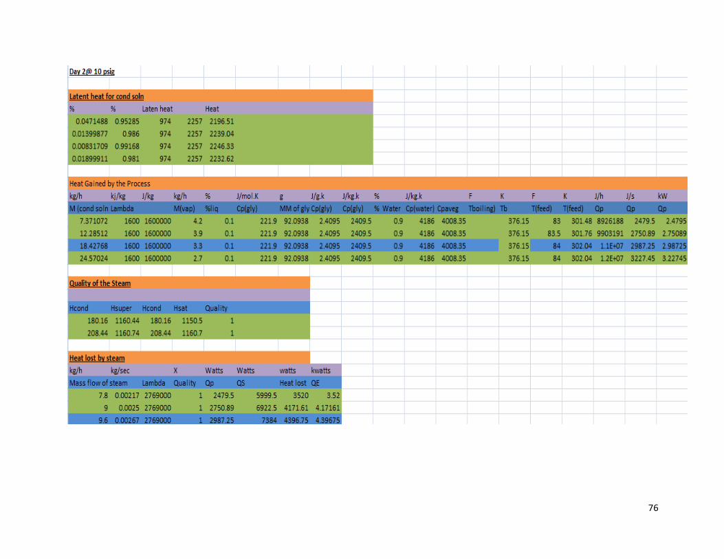
76

77

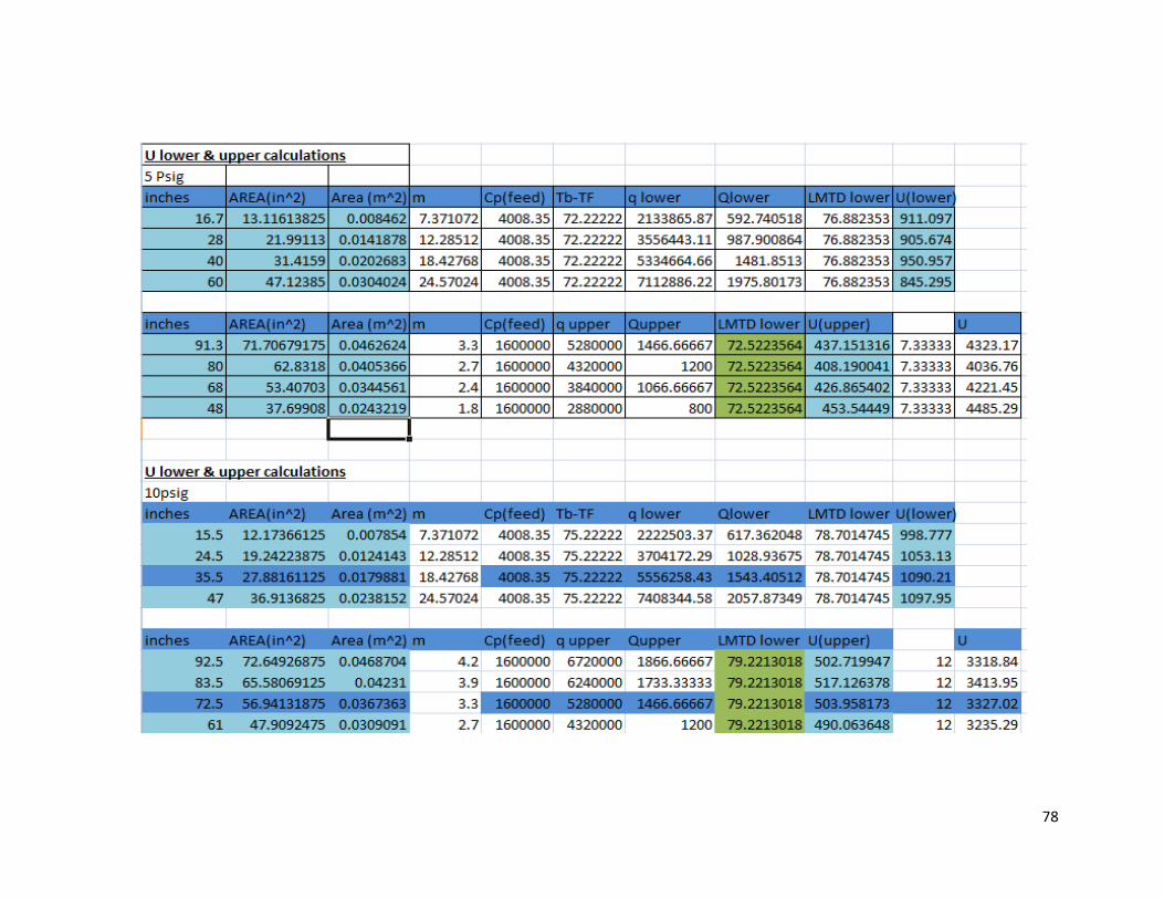
78

79