Embed Size (px)
Citation preview

1
Project Narrative (≤20 pages)
1. Background/Introduction
Shallow and deep convection strongly interact with large-scale atmospheric processes and local land surface, atmospheric boundary layer (ABL), and aerosols. They also strongly affect precipitation and the radiative balance of the atmosphere and land surface. The understanding and model representation of convective processes have been improved in recent decades; for instance, as reflected by the rapidly expanding number of publications using the ARM facilities and data. In fact, a simple search (on 1 January 2016) of journal articles with words “ARM” and “convective” yield 445 and 148 articles, respectively, from the ARM publications database (http://www.arm.gov/publications/db).
This improved understanding and model representation of convective processes are also reflected by the evolution of parameterizations of relevant processes in the atmospheric component of the Community Earth System Model (CESM), the Community Atmospheric Model (CAM), which is the basis of the atmospheric component of version 0 of the DOE Accelerated Climate Model for Energy (ACME). For instance, in the current version 5 (CAM5), the previous ABL turbulence scheme (Holtslag and Boville 1993) was replaced by a moist turbulence scheme that can be applied anywhere in the atmosphere where the moist Richardson number is greater than a critical value (Bretherton and Park 2009). Additionally, a new shallow convection parameterization (Park and Bretherton 2009) that works with this new moist turbulence scheme was implemented. While the parameterization of deep convection (Zhang and McFarlane 1995) was retained, it has been improved over the years by the inclusion of convective momentum transport (Richter and Rasch 2008) and of moist entropy conservation and mixing methods by Raymond and Blyth (1986, 1992). Convection and microphysics were further refined in CAM5.5 by the inclusion of an updated large-scale microphysics (Gettelman and Morrison 2015) and the Cloud Layers Unified by Binormals (CLUBB) scheme (Golaz et al. 2002; Larson et al. 2012; Bogenschutz et al. 2012) which would unify the turbulence, shallow convection, and large-scale clouds. While CLUBB is preferred for both CAM6 and ACME1, the Unified Convection Scheme (UNICON, Park 2014), which would unify shallow and deep convection, is still being considered for inclusion.
Despite this progress, two critical knowledge gaps and challenges remain:
Overarching Question (OQ) 1: What are the different roles of wind shear in convective precipitation over midlatitude versus tropical land?
OQ2: What are the diurnal and seasonal variations of the land-convection interactions and the responsible mechanisms over midlatitude versus tropical land?
For the OQ1, the effect of vertical wind shear (VWS), defined as the difference between the wind vectors at different heights, on convective development has been studied for decades (e.g., Pastushkov 1975; Cotton and Anthes 1989). VWS affects convection through the modification of the vertical transport of horizontal momentum (e.g., Wu and Yanai 1994). It is also well known that VWS has a negative correlation with intensity change in tropical cyclones at all stages of their life cycle (Gray 1968).
In an environment without shear, convective downdrafts bring low-entropy air from the mid-troposphere down to near the surface, which then forms a surface-based cold pool. This is detrimental to further convective development by cutting off the supply of relatively warm and moist air, so that isolated cumulus clouds usually form over mid-latitude land under such a condition.
When the environment is sheared (in wind magnitude or direction), the cold pool does not overlap with the updraft region of the convection and hence does not cut off the supply of moisture. Furthermore, the cold pool can propagate horizontally as a density current which uplifts environmental boundary layer air to its level of free convection and may trigger new convective cells. Therefore, when the VWS in the lower troposphere is weak, single cell and short-lived storms occur. When the VWS is moderate, multicell storms (with a total storm lifetime of many hours) arise; when the VWS is even stronger, a supercell

2
storm may develop, often producing heavy rain, hail, and damaging tornadoes (Cotton and Anthes 1989; Holton 2004). In contrast, a strong VWS is unfavorable for tropical cyclone initiation and development (e.g., Emanuel 1994).
Fan et al. (2009) also found that VWS plays a dominant role in regulating aerosol effects on isolated deep convective clouds: increasing aerosol loadings suppress convection under strong wind shear and invigorate convection under weak wind shear until this effect saturates at an optimal aerosol loading. They suggested that the physical basis for the difference in the two wind shear conditions was rooted in the competition between condensational heating and evaporative cooling as a function of aerosol loading.
Despite its importance, the effect of VWS on convection has largely been ignored in parameterization schemes for large-scale models (e.g., Liu and Moncrieff 2001). The only exception is in regard to convective momentum transport (Richter and Rasch 2008) which was added to the CAM5 deep convection scheme. Liu and Moncrieff (2001) also found that convective heating and drying, mass fluxes, and cloud fraction are greatly impacted by VWS. These effects still have not been included in the CAM5 convective parameterizations which may cause biases in quantities that directly regulate energy balance, such as cloud fraction, optical depth, and radiative fluxes (e.g., Anber et al. 2014).
Motivated by these and other observational and modeling studies, two questions can be raised:
What is the relationship between VWS and convection over the midlatitude versus tropical land based on field campaign and long-term comprehensive ARM data?
Over these two regions, how does the DOE ACME model perform against the above observational analyses?
For the OQ2, land and atmosphere interact with each other at diurnal, seasonal, and longer time scales. Convective precipitation over continental areas usually has a large diurnal variation, most commonly peaking in the afternoon, as expected from local vertical thermodynamic processes. However, it also has a nocturnal maximum in some locations, most notably over the U.S. Southern Great Plains (SGP) (including the ARM SGP sites) in summer (Wallace 1975; Balling 1985; Higgins et al. 1997). This nocturnal maximum of precipitation may be attributed to three main forcings: i) the passage of eastward-propagating rainfall systems with origins near the Continental Divide; ii) a nocturnal reversal of the mountain–plains circulation (which is associated with widespread nighttime ascent over the plains); and iii) the transport of energetic air and moisture convergence by the SGP low-level jet (LLJ) (Carbone et al. 2002; Jiang et al. 2006; Carbone and Tuttle 2008).
Carbone et al. (2002) found that the phase speed of precipitation episodes commonly exceeds the phase speed of upper tropospheric anomalies and often exceeds zonal steering winds in the low- to mid-troposphere, which is suggestive of a convectively generated propagation mechanism. Furthermore, Matsui et al. (2010) found that rainfall horizontal propagation speeds are better linked to the convective available potential energy (CAPE) than to ABL dryness.
Most current global and regional climate models show deficiencies in reproducing the nocturnal precipitation signal over the Great Plains primarily due to deficiencies in the deep convection scheme (e.g., Dai et al. 1999; Liang et al. 2004). Lee et al. (2007) also suggested that improvements to the diurnal cycle in their model require improvements to the parameterized deep convection scheme, including the coupling with the ABL, the characteristic timescale of convection adjustment, and the triggering process for nocturnal precipitation. Dirmeyer et al. (2012) found that increasing resolution alone (from a grid spacing of 125 km to 39 km and 16 km) has little impact on the timing of daily rainfall in the European Centre for Medium-range Weather Forecasts (ECMWF) model with parameterized convection, yet the amplitude of the diurnal cycle does improve along with the representation of mean rainfall. They also suggested that the distinctive treatments of model physics accounted for the differences in representing the diurnal cycle of precipitation among different models.

Fmoisture)precipitatiprevious precipitatidifferent precipitatiBrubaker and Bras al. 2006; isotope dKurita etvapor traDruyan Bosilovic2002); idpathways precipitatiDirmeyer land-precistrength 2010). Inparameteret al. (201and usefuthe resultregional r
TnumerousAtmospheanomalies2006; Guoof land-atWang et a
Aperspectivframeworand Eltahthe precievapotrandaytime Aand Barrointeractionthe SGP rmorning etriggeringfrequency
M
Figure 1 summ, ABL (turbion at differe
studies onion couplin
cation recyclinget al. 1993;
1996; DominLamb et al.
data analysit al. 2004);acer analysisand Koster h and Sdentification
for the ion coupling
et al. 200ipitation c(e.g., Zeng
n particular, tr proposed b10) provides aul index to qts from glob
reanalyses as w
To directly adds studies. In ere Coupling s in land surfo et al. 2006)tmosphere coal. 2007; Nota
At shorter tives. For instark to diagnosehir (2003) foupitation, dep
nspiration andABL growth. os (2014) usns can influenregion. Airesenvironmentag potential, any and intensity
Motivated by t
marizes the rbulent mixinent time sca
n land-ng into egories: g (e.g.,
Eltahir nguez et . 2012); s (e.g., ; water s (e.g.,
1989; Schubert
of the land-
g (e.g., 9); and
coupling et al.
the new by Zeng a simple quantify bal and well as region
dress the landparticular,
Experiment face (e.g., so. While theseoupling, sevearo 2008; Zha
ime scales, ance, Santanee the contribu
und that soil mpending on td hence moistFurthermore,sed a regionnce the eastws et al. (2014al conditions (nd low-level y.
these and othe
FBB
relevant mechng), atmosphles. At mont
nal and globa
d-precipitationtwelve globa(GLACE) thil moisture) c
e GLACE studeral limitationang et al. 200
land-atmospello et al. (20utions from smoisture anomthe atmosphten the ABL,, the ABL top
nal model toward propagati4) developed (as representehumidity de
er observation
Figure 1. SchBetts and SilvBetts et al. (1
3
hanisms involheric dynamithly and sea
al climate mod
n coupling, real modeling hat focused ocan affect sudies representns have also 8).
here interac009, 2011) dsurface energymalies may peric profile: , while decrep entrainment
o evaluate wion of nocturna framework
ed by the surfficit) and sub
nal and mode
hematic of lanva Dias (20101996).
lving land (vics, and aer
asonal scales,
deling.
egional and ggroups part
on the quantifummertime rat a crucial advbeen noted
ctions have developed a ly fluxes and produce a pos
wet soil meased sensiblet is also impo
whether and hnal deep convk to evaluate face turbulentbsequent afte
eling studies,
nd-surface-atm0) as an updat
vegetation, sorosols, cloud, Zeng et al.
global modelsticipated in fication of thainfall generavancement in(e.g., Senevi
been studielocal land-atmentrainment sitive or a ne
moisture maye heat flux mortant for ABhow daytimevection in the
the relationst fluxes partiternoon conve
three question
mosphere coute of the origi
oil temperaturds, radiation,. (2010) clas
s have been uthe Global L
he degree to wation (Koster n the understairatne et al.
ed from difmosphere coufrom aloft. F
egative respony increase sumay slow dowBL growth. Ere land-atmos
e warm seasonship between tioning, convective precipi
ns can be rais
upling from inal figure in
re and , and ssified
sed in Land-which et al.
anding 2006;
fferent upling
Findell nse in urface
wn the rlingis sphere n over
early ective itation
sed:

4
What is the co-evolutionary nature of all relevant features (land, ABL, aerosols, clouds, radiation, and precipitation) at diurnal and seasonal time scales over midlatitude versus tropical land?
What are the processes responsible for the diurnal and seasonal variations of key quantities?
How does ACME perform against the above observational analyses over these regions?
Relevant to these OQs are aerosol-cloud-precipitation interactions, which are linked to the largest single source of uncertainty in current estimates of the total anthropogenic radiative forcing (IPCC 2013). Beyond the direct effect of aerosols on climate via interactions with solar radiation, aerosols also indirectly affect climate due to their role in altering cloud properties. The physical basis for aerosol effects on cloud microphysics and precipitation rests on three principles: (i) an increase in aerosol results in more numerous, but smaller droplets (all else being equal) (Twomey 1977); (ii) the collision-coalescence efficiency between these small droplets is significantly reduced and therefore the primary warm rain precipitation-generation mechanism is suppressed (Warner 1968; Albrecht 1989); and (iii) the efficiency of riming of these small droplets by ice particles is significantly reduced (Borys et al. 2000; Saleeby et al. 2013). The relationship between aerosols and deep convective clouds is even more complex with evidence that under certain conditions aerosol particles of varying physicochemical nature can invigorate convection and even increase rainfall (Khain et al. 2005; Lynn et al. 2005; Seifert and Beheng 2006; van den Heever et al. 2006; Khain 2009).
Our strategy here is to include aerosols as an integrated part of our efforts in addressing the above OQs (rather than focus on the aerosol-cloud-precipitation interactions themselves); this effort is further motivated by recent findings demonstrating that there is a complex interconnection between wind shear, aerosol particles, convective strength, and cloud properties (e.g., Lee et al. 2008; Fan et al. 2009). Relevant to these OQs is the evaluation of the atmospheric and land model components of the ACME and pathways for model improvement.
Our objectives will be presented in Section 2, while the relevance of the proposed work to DOE will be discussed in Section 3. The data and model will be described in Section 4.1. The two overarching questions (OQs) will be addressed in Sections 4.2-4.4, and the uncertainty quantifications will be presented in Section 4.5. Deliverables, management, and timeline will be presented in Section 4.6.
2. Project Objectives
Our overall objectives are: (a) to address these OQs using the ARM data over midlatitude and tropical continents, and (b) to evaluate and improve the representation of convective processes in the DOE ACME model. Direct measurements and value-added ARM data from the MC3E and GOAmazon field campaigns, and long-term comprehensive ARM data at the SGP sites will be used. Complementary in situ and satellite data as well reanalysis data will also be used. Our objectives will be addressed through three data-model integrated tasks along with uncertainty quantifications:
Task 1 (Section 4.2): to quantify the diurnal and seasonal variations of land-convection interactions over midlatitude versus tropical land (including any time-delayed relationship) from observations and to document the ACME model deficiencies;
Task 2 (Section 4.3): to quantify the differing roles of vertical shear of horizontal wind vector in convective precipitation over midlatitude versus tropical land (including the favorable environmental conditions for shallow and deep convection initiation and development) from observations and to document the ACME model deficiencies; and
Task 3 (Section 4.4): to quantify the contribution of individual processes to key quantities (e.g., liquid and ice water content and aerosol) through data analysis and model sensitivity tests and to provide the pathways for ACME model improvement.

5
3. Relevance to the DOE ASR program
The scientific benefits of this project are represented by the two final deliverables: (a) a better understanding of convective processes by quantifying the role of vertical wind shear and local land-atmosphere interactions in convective processes; and (b) pathways for improved model representation of convective and related processes over different climate regimes through atmospheric variable budget analysis and model sensitivity tests.
This project directly addresses “convective processes using results from ARM campaigns” – one of the four focus areas of this DOE Funding Opportunity Announcement (FOA). Our evaluations of the DOE ACME model for its improvement in the convective processes are consistent with the priorities in the FOA. The project also directly addresses two goals [“Synthesize new process knowledge and innovative computational methods advancing next-generation, integrated models of the human-Earth system” and “Enhance the unique capabilities and impacts of the ARM and EMSL scientific user facilities and other BER community resources to advance the frontiers of climate and environmental science”] of the DOE Climate and Environmental Science Division (CESD).
4. Proposed Research and Methods
We will address the above objectives through three tasks in Sections 4.2-4.4. As a data-model integrated project, both data analysis and modeling will be emphasized in each task. Uncertainty quantifications (Section 4.5) will also be emphasized in each task. First, Section 4.1 presents the data and model that will be used in our research.
4.1 ARM data and model descriptions
ARM data. Unlike other types of observational datasets, ARM provides the advantage of a high inventory of in-situ data over our regions of interest to examine relationships such as (but not limited to) between aerosols and convection as a function of other environmental factors (e.g., humidity, wind shear, and aerosol properties). We will make extensive use of the ARM field campaigns data from MC3E (Midlatitude Continental Convective Clouds Experiment) over the Southern Great Plains (SGP) during the April to May 2011 period and GOAmazon (Green Ocean Amazon) over the Amazon from January 2014 to December 2015.
MC3E (http://www.arm.gov/campaigns/mc3e/) was a joint field program involving NASA Global Precipitation Measurement (GPM) Program and ARM investigators. The experiment leveraged the unprecedented observing infrastructure available in the central United States, combined with an extensive sounding array, to provide a complete characterization of convective cloud systems and their environment. Several different components of convective processes tangible to the convective parameterization problem were targeted, such as pre-convective environment and convective initiation, updraft/downdraft dynamics, condensate transport and detrainment, precipitation and cloud microphysics, influence on the environment and radiation, and a detailed description of the large-scale forcing. The intensive observation period used a new multi-scale observing strategy with the participation of a network of distributed sensors (both passive and active). The approach was to document in 3D not only precipitation, but also clouds, winds, and moisture in an attempt to provide a holistic view of convective clouds and their feedback with the environment. Both ground-based and airborne measurements are available. Value-added data, including the single-column model forcing data developed by our project collaborator Shaocheng Xie, are also available (https://www.arm.gov/campaigns/sgp2011midlatcloud).
GOAmazon (http://campaign.arm.gov/goamazon2014/) was a DOE-supported field campaign over the Amazon in collaboration with Brazilian and German organizations to better understand the coupled atmosphere-cloud-terrestrial tropical systems. The experiment was designed to enable the study of how aerosols and surface fluxes influence cloud cycles under clean conditions, as well as how aerosol and cloud life cycles, including aerosol-cloud-precipitation interactions, are influenced by pollutant

6
outflow from a tropical megacity. Both ground-based and airborne measurements are available. We have done preliminary analysis of these field campaign data, and as an example, Figure 2 shows the seasonal cycle of various atmospheric variables over the Amazon.
Besides these field campaign data, we will also use the long-term comprehensive ARM data at the Southern Great Plains (SGP) sites (https://www.arm.gov/sites/sgp). This was the first field measurement site in north-central Oklahoma established by the ARM Program with measurements starting from 1992. More than 30 instrument clusters have been placed at the SGP Central Facility and at Boundary, Extended, and Intermediate Facilities. These data include: 1) aerosol physicochemical characteristics, 2) cloud geometry and water content, 3) thermodynamic and wind profiles (including ABL height), 4) precipitation type, amount and drop size distribution, 5) surface meteorology, radiation and turbulent fluxes, and 6) soil moisture and temperature.
Considering the large amount and large variety of ARM data available, we will focus on value-added products. Only when such products are not available, will we use data from direct measurements (e.g., various aerosol quantities). Airborne ARM data are not central to the project and will only be used as needed for case studies of potential interest. We will use the value-added ARM best estimate (ARMBE) data product developed by our collaborator (Shaocheng Xie) (Xie et al. 2010) for model evaluations. This dataset contains information on the atmosphere, wind, clouds, radiation, precipitation, latent and sensible heat fluxes, and were obtained using the different instrumental observations covering the periods 1994-2012 for SGP. Xie’s group has also developed the gridded and station based surface/land data at SGP for the MC3E field campaign period of April-June 2011(www.arm.gov/data/eval/94), which will also be used.
Complementary data. Besides the ARM data, we will also use the hourly 4 km radar/gauge merged Stage-IV precipitation data (Seo 1998; Lin and Mitchell 2005) over the U.S. Such data and 120 rain gauge data over a 200 km × 200 km area within the state of Ohio have been used in our previous study (Kursinski and Zeng 2006) to address the precipitation spatial heterogeneity issue.
Over the Amazon, there is a low density of surface precipitation measurement instruments (e.g. rain gauges and weather radar). In order to obtain information on the larger scale characteristics and propagating nature of precipitation, we will use the 3-hourly 0.25° TRMM satellite data (since 1998; Kummerow et al. 2000) and the 0.5-hourly 0.1° x 0.1° Integrated Multi-satellitE Retrievals for GPM (IMERG) satellite data. These datasets have been used before within this region and were able to provide
Figure 2. Example of GOAmazon observations. Top panel: Relative humidity in lowest 10 km of the atmosphere (from rawinsondes). Lower panel: Wind direction and speed at 5-km elevation (from rawinsondes), rainfall intensity (from rain gauge) and CCN observations (from the Aerosol Observing System, AOS). Blue and red rectangles in the lower panel indicate hot-wet and hot-dry season, respectively, as used in Figs. 4 and 5.

7
reasonable precipitation estimates in comparison with a large-scale rain gauge network (Buarque et al. 2011; Clarke et al. 2011).
Furthermore, we will use the Modern Era Retrospective-analysis for Research and Applications version 2 (MERRA2) (Bosilovich et al. 2015; Rienecker et al. 2011) from 1979 to present at 0.5° latitude x 0.625° longitude grids with 72 vertical layers from the surface up to 0.01 hPa. Its modeling components include the Goddard Earth Observing System (GEOS-5) atmospheric general circulation model (Lucchesi 2012) coupled with the Catchment land model (Koster et al. 2000), as driven by observed sea surface temperature and sea ice (Reynolds and Smith 1995). MERRA2 provides hourly two-dimensional fields (typically surface and top of the atmosphere fields) at 0.5° x 0.625° grids and 3-hourly three-dimensional fields also at 0.5° x 0.625° grids on 42 pressure levels (Lucchesi 2012). These latter fields include tendencies of atmospheric quantities. For quantities like specific humidity and temperature, the contribution from the analysis increment is also included. All of these tendencies are also provided for vertical integrals of various quantities. MERRA has been extensively evaluated (e.g., see the MERRA Special Collection in Journal of Climate: http://journals.ametsoc.org/page/MERRA), including using the ARM data (e.g., Kennedy et al. 2011).
In this project, we will use the MERRA2 reanalysis data for atmospheric budget analysis (in Section 4.4) and to quantify large-scale weather patterns for all tasks. The availability of individual contributions to various tendencies is a major reason for using MERRA2 (rather than other reanalysis products). MERRA products have been widely used in our prior research (e.g., Wang and Zeng 2013; Brunke et al. 2014).
ACME model. ACME is a modeling project launched by DOE in July 2014 to develop a branch of the CESM to advance a set of science questions for the near-term time horizon (1970-2050) based on high resolution coupled climate simulations (15-25 km), with adaptable grids <10 km, using advanced software and the next and successive generations DOE Leadership Class computers, both hybrid and multi-core, through exascale (http://climatemodeling.science.energy.gov/projects/accelerated-climate-modeling-energy). Over 100 researchers are involved in ACME model development, with most of them from eight DOE Laboratories. This project is particularly relevant to one of the three science drivers for the ACME development (Water cycle: How do the hydrological cycle and water resources interact with the climate system on local to global scales? What are the processes and factors governing precipitation and the water cycle today and how will precipitation evolve over the next 40 years?).
ACME Version 0 (ACME0) is based on CESM1, and ACME1 has been frozen for evaluation and tuning and will be released in 2017. At the same time, ACME2 is under development now. Our team was just approved by the ACME Council in December 2015 to become an official ACME collaborator with access to the ACME codes (expected in late January 2016). This approval and the inclusion of Ruby Leung (ACME Chief Scientist) and Shaocheng Xie (ACME Atmospheric Model Co-Lead) as our project collaborators give us the confidence that we will be able to get access to the ACME codes and model outputs from day 1 of this project. Furthermore, we are very familiar with CESM (which is the basis of ACME). PI Zeng was the coordinator for the development of the initial version of CLM (Zeng et al. 2002; Dai et al. 2003), and his group has also been heavily involved in the subsequent CLM development. Therefore, we decide to focus on ACME in this project and hence directly contribute to this new DOE modeling initiative, even though many details of ACME remain unclear at present.
The ACME atmospheric model is based on the scalable spectral element dynamical core for the CAM5 (Dennis et al. 2011). ACME will also include improved aerosols and clouds over CAM5 (e.g., aerosol deposition on ice and snow; convective aerosol transport, activation, removal). While UNICON was preferred at the ACME All-Hands Fall Meeting in November 2015 (where PI Zeng attended as an ACME collaborator), CLUBB is preferred for ACME1 right now (Phil Rasch, personal communication, January 2016). For our project, we will evaluate ACME results with both CLUBB and UNICON. As an example, Figure 3 illustrates the physical processes in UNICON. In contrast to the traditional regime-

8
dependent parameterization in Fig. 3a, local transport is parameterized by a moist turbulence scheme in CAM5 that simulates both dry and saturated turbulent transport in all atmospheric layers (Fig. 3b). The remaining non-local transport is performed by UNICON that consists of three parts: (a) subgrid convective updrafts originating from the surface, typically in an unsaturated state, but that eventually become saturated above the lifting condensation level (LCL) with corresponding compensating subsidence; (b) subgrid convective downdrafts that are generated from convective updrafts and can penetrate into ABL when sufficiently cooled by evaporation of convective precipitation; and (c) subgrid mesoscale organized flow driven by convective downdrafts and evaporation of convective precipitation, which feeds back to convective updrafts.
The ACME Land Model (ALM) is based on the Community Land Model (CLM; Oleson et al. 2013) with improvements in hydrology (e.g., watershed delineation), biogeochemistry (e.g., competition representation for nutrients N and P), and vegetation (e.g., root and leaf traits for nutrient acquisition and use).
4.2 Diurnal and seasonal variations of land-convection interactions (Task 1)
First we will analyze the summertime hourly precipitation diurnal cycle using the ARM SGP data and the MC3E data, precipitation propagation using the Stage-IV precipitation data following previous studies (e.g., Carbone et al. 2002; Jiang et al. 2006; Carbone and Tuttle 2008; Matsui et al. 2010), and large-scale convergence and synoptic weather pattern using the MERRA2 data in Task 1. These analyses will then be expanded to the GOAmazon sites where datasets are less comprehensive than those at the SGP sites. These analyses will quantify the differences in precipitation diurnal cycle and propagation in different climate regimes.
There are two unique aspects of our analysis in Task 1: one is the inclusion of the precipitation propagation that enables us to document the relative contributions of horizontal propagation of precipitation versus local vertical column processes to the precipitation diurnal cycle climatology in the ARM hourly precipitation data over these regions; another is to repeat the above analyses for the convective and stratiform precipitation separately. Previous studies emphasized the diurnal cycle of total precipitation (e.g., Matsui et al. 2010) and radar reflectivity (e.g., Carbone et al. 2002; Carbone and Tuttle 2008). Convective and stratiform precipitation generally differ in vertical wind velocity, rainfall intensity (largest for convective), microphysics, latent heating and temporal extent (Houze 1993; Yuter and Houze Jr. 1995; Hazenberg et al. 2014), and diurnal cycle (e.g. Berenguer et al. 2012; Giangrande et al. 2014). Significant progress has been made to separate total precipitation into its convective and stratiform
Figure 3. Diagrams illustrating subgrid vertical transport in atmospheric models with (a) the traditional view in CAM5 and (b) the alternative view that is adopted by UNICON with CAM5 (Fig. 1 in Park 2014).

9
components (Tokay and Short 1996; Bringi et al. 2003; Lang et al. 2003; Hazenberg et al. 2014). This has also been applied at the different ARM sites (Lang et al. 2003; Giangrande et al. 2013, 2014; Deng et al. 2014). Co-I Hazenberg has worked with both volumetric radar data as well as in situ observations (both rain gauge and disdrometer) to differentiate convective and stratiform rainfall. Many of these methods use the information from both cloud and precipitation radar information and surface disdrometer and rain gauge measurements.
We will do this analysis in Task 1 by using the MC3E campaign datasets (including video and Parsivel disdrometer data, radar data, and 3D wind fields derived from radar measurements; all available at http://www.arm.gov/campaigns/sgp2011midlatcloud). If needed, we may also use additional measurements at the SGP sites (e.g., the value added K-band scanning cloud radar KAZR corrected data, the Precipitation Radar Moments mapped to a Cartesian grid, and Scanning ARM Cloud Radar Corrections (SACRCOR) products). For the GOAmazon campaign, differentiation between convective and stratiform precipitation will be obtained using vertically scanning radar observations (i.e., radar wind profiler, W-band ARM cloud radar WACR) and surface observations (i.e., Parsivel laser disdrometer, rain gauge, and surface meteorological instrumentation).
In Task 1, we will also quantify the relationship of precipitation with drop size distribution (DSD) using the disdrometer observations (impact and video disdrometer). As an example, Figure 4 shows the seasonal variability of this relationship as observed during the GOAmazon campaign. Furthermore, precipitation rate is closely related to the vertical evolution of the raindrop size distribution under influences of 1) collision-induced breakup and coalescence processes, 2) aerodynamic breakup and the impact of up- and down-drafts (Young 1975; Testik and Barros 2007), and 3) below-cloud evaporation (Rosenfeld and Ulbrich 2003; Kumjian and Rhyzkov 2010). The last process would result in a reduction of the number of small droplets and overall water content of precipitation, while evaporative cooling can result in the generation of downdrafts (Srivastava 1985, 1987; Kumjian and Rhyzkov 2010). To better understand the impact of this, we will make use of the value added data (K-band scanning cloud radar KAZR corrected for SGP and WACR observations for GOAmazon).
Such analyses of precipitation will enable us to address many first-order questions such as: What is the difference in the diurnal cycle of stratiform and convective precipitation? How does this change with season (as seen in Fig. 4 for the Amazon)? What is the difference in the relative contributions of horizontal versus vertical processes to stratiform and convective precipitation?
To address the seasonal cycle, we will also do a detailed analysis of processes and parameters that contribute to the averaged diurnal cycle of clouds and precipitation in each month from spring to summer and to fall over the SGP sites in Task 1. For instance, the nocturnal precipitation maximum over the SGP region is most pronounced in mid-summer (June and July) (e.g., Carbone et al. 2002). Over tropical land,
Figure 4. Distribution of observed DSD concentration and the shape parameter μ and slope parameter λ (Brawn and Upton 2008) of the gamma distribution used to represent the DSD distribution. Results are based on the GOAmazon Parsivel laser distrometer measurements correcting with Raupach and Berne (2015) for convective precipitation with 1-minute intensity >10 mm h-1 (Uijlenhoet et al. 2003).
10
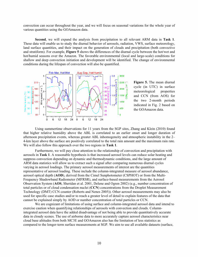
convection can occur throughout the year, and we will focus on seasonal variations for the whole year of various quantities using the GOAmazon data.
Second, we will expand the analysis from precipitation to all relevant ARM data in Task 1. These data will enable us to study the diurnal behavior of aerosols, radiation, VWS, surface meteorology, land surface quantities, and their impact on the generation of clouds and precipitation (both convective and stratiform). For example, Figure 5 shows the differences of the diurnal cycle between the hot/wet and hot/humid seasons over the Amazon. The favorable environmental (local and large-scale) conditions for shallow and deep convection initiation and development will be identified. The change of environmental conditions during the lifespan of convection will also be quantified.
Using summertime observations for 11 years from the SGP sites, Zhang and Klein (2010) found that higher relative humidity above the ABL is correlated to an earlier onset and longer duration of afternoon precipitation events, whereas greater ABL inhomogeneity and atmospheric instability in the 2–4-km layer above the surface are positively correlated to the total rain amount and the maximum rain rate. We will also follow this approach over the two regions in Task 1.
Furthermore, we will pay close attention to the relationship of convection and precipitation with aerosols in Task 1. A reasonable hypothesis is that increased aerosol levels can reduce solar heating and suppress convection depending on dynamic and thermodynamic conditions, and the large amount of ARM data statistics will allow us to extract such a signal after comparing numerous diurnal cycles varying in aerosol loadings. The primary aerosol measurements of interest are the quantities representative of aerosol loading. These include the column-integrated measure of aerosol abundance, aerosol optical depth (AOD), derived from the Cimel Sunphotometer (CSPHOT) or from the Multi-Frequency Shadowband Radiometer (MFRSR), and surface-based measurements from the Aerosol Observation System (AOS, Sheridan et al. 2001, Delene and Ogren 2002) (e.g., number concentration of total particles or of cloud condensation nuclei (CCN) concentrations from the Droplet Measurement Technology (DMT) CCN counter (Roberts and Nenes 2005)). Other aerosol measurements may also be used for specific case studies and/or to reach a greater level of detail to explain features of the data that cannot be explained simply by AOD or number concentration of total particles or CCN.
We are cognizant of limitations of using surface and column-integrated aerosol data and intend to exercise caution when quantifying relationships of aerosols with convection and clouds. Column-integrated aerosol data have the added disadvantage of not being able to provide quantitatively accurate data in cloudy scenes. The use of airborne data to more accurately capture aerosol characteristics near cloud base altitudes from both MC3E and GOAmazon also has the limitation of less statistics as compared to the longer-term surface measurements at SGP. We aim to use all available datasets (surface,
Figure 5. The mean diurnal cycle (in UTC) in surface meteorological properties and CCN (from AOS) for the two 2-month periods indicated in Fig. 2 based on the GOAmazon data.

11
airborne, reanalysis, satellite) to rely on the strengths of each tool to robustly calculate aerosol-convection interactions as they relate to cloud processes and precipitation.
Diurnal profiles of aerosol characteristics have been documented already at both the SGP and Amazon sites, giving us confidence in the high potential of finding a relationship between aerosol loading and convection. As an example for the SGP sites, Iziomon and Lohmann (2003) used multi-year data to show a pronounced diurnal cycle of submicron aerosol concentration, with minimum and maximum amounts in the morning and afternoon, respectively. At the GOAmazon site, a number of studies have examined how environmental parameters vary seasonally and diurnally. Aerosol concentrations and sources differ markedly between the dry (~June – October) and wet seasons (~February – May) (see Fig. 5), with biomass burning and fossil-fuel combustion emissions being more significant in the former, leading to higher concentrations and scattering and absorption coefficients (Andreae et al. 2015).
Third, we will run ACME driven by the observed sea surface temperature and sea ice from 2011-2015 to cover the periods of both MC3E (in 2011) and GOAmazon (in 2014-2015) in Task 1. ACME has already set up various protocols for ACME simulations, including ACME simulations at the development resolution of 100 km (in the horizontal direction) with 30, 64, and 72 vertical layers and production resolution of 25 km (in the horizontal direction) with 72 vertical layers and the model top at ~60 km. If the model outputs at hourly (or at least 3-hourly) frequency are available, we will compare them with the above observational data.
If such high-frequency outputs are unavailable, we will repeat the simulations ourselves at three horizontal and vertical resolutions (with all model simulations summarized in Table 2 in Section 4.5):
Base simulation (Test0) at 25 km with 72 layers (same as the ACME production resolution)
Sensitivity Test1 at 100 km with 72 layers (same as one ACME development resolution)
Sensitivity Test2 at 100 km with 30 layers (same as another ACME development resolution)
We have done similar simulations extensively in the past (e.g., Barlage and Zeng 2004). We will then save hourly output of relevant variables for all tasks. We will pay particular attention to the following issues in our model-data comparisons.
It is well known that coarse-resolution global models (e.g., with 100 km grid boxes) have difficulty in realistically simulating the propagation of convective precipitation. Therefore, we will explore in Task 1 how the quadrupling of resolution would affect the propagation of convective precipitation in ACME (based on Test0 versus Test1).
Besides the diurnal precipitation timing, the precipitation intensity and frequency will also be emphasized, as motivated by our previous data analyses (e.g., Chen et al. 1996; Kursinski and Zeng 2006; Stillman et al. 2013).
Furthermore, because global models treat stratiform and convective precipitation separately, we will compare the diurnal cycle of stratiform and convective precipitation in ACME with observations. The dependence of these model results on the model horizontal resolution will also be explored (based on Test0 versus Test1).
Lee et al. (2008) examined the role of convection triggers in the simulation of the diurnal cycle of precipitation over the Great Plains in a climate model, and found that the nighttime elevation of the convection starting level (defined as the maximum level of moist static energy from the surface) above the ABL inversion provides the condition favorable for the development of nocturnal precipitation. Lee et al. (2007, 2008) also found that convection schemes sensitive to upward motion produce the nocturnal maximum, but those responding primarily to surface heating simulate only afternoon peaks. This issue will also be addressed using ACME.
Motivated by these studies, we hypothesize that vertical resolution will be important in capturing nocturnal convection when the ABL is shallow. Also, there is a need for consistent vertical and horizontal

12
resolutions (Lindzen and Fox-Rabinovitz 1989). We will then test this hypothesis by comparing results from Test0, Test1, and Test2 with observations and prior studies (e.g., Lee et al. 2007, 2008) in Task 1.
Besides the model sensitivity to horizontal and vertical resolutions, we will also address the impact of aerosols on convective processes by comparing the base simulation (Test0) with modern-era (~year 2000) emissions against a sensitivity run [Test3, same as Test0 except using pre-industrial (~year 1850) emissions] in Task 1. This is similar to what was done by Gettelman et al. (2013).
Through these model evaluations, we hope to gain insights on model deficiencies in Task 1. For instance, we have analyzed the hourly output of an earlier version of the NCAR climate model and found that the model contained a spurious cycle: too much drizzle was produced; the drizzle then evaporated in the ABL, never reaching the surface for soil moisture; and this maintained a relatively moist ABL, producing drizzle again. An interesting question we will address is: does ACME have an excessive drizzle problem? Does the model treat the below-cloud evaporation properly? These analyses and the insights gained through them will provide the basis for subsequent tasks.
4.3 The different roles of wind shear in convection over midlatitude versus tropical land (Task 2)
First, we will analyze the hourly precipitation data for individual storm events from late spring to early fall versus the vertical wind shear (VWS) in the lower troposphere using the MC3E and SGP data in Task 2. The GOAmazon data for the entire year will also be analyzed. VWS here includes the vertical difference of both horizontal wind magnitude and direction. Both instrumental (i.e., wind profiler and sounding data) as well as MERRA2 reanalysis data will be applied for this task. We will pay particular attention to the following questions:
What is the relationship between VWS and precipitation (amount and intensity) over the SGP and GOAmazon sites?
Does the relationship change between daytime and nighttime over the SGP and GOAmazon sites?
How does the relationship change from the SGP sites (over midlatitudes) to the GOAmazon sites (over tropics)?
What are the appropriate levels (e.g., between first model level above surface and 850, 700, 600, or 500 mb; between 900 mb and 700, 600, or 500 mb) to define VWS (in both magnitude and direction)?
For instance, Figure 6 shows that the mean wind shear at SGP for 5.5 days in April 2011 during MC3E is higher than it generally is in the Amazon at ~5 m s-1 km-1. Precipitation tends to be higher during for 24 and 25 April when maximum wind shear is at its highest. The value-added ARM best estimate product (Xie et al. 2010) would be best-suited for such an analysis. As this is only available at the SGP Central Facility, we will also have to rely on rawinsondes from MC3E and GOAmazon and the surface meteorological instrumentation at SGP Extended Facilities and GOAmazon.
Second, the favorable environmental (local and large-scale) conditions for shallow and deep convection initiation and development will be identified in Task 2. The change of environmental conditions during the lifespan of convection will also be quantified. As mentioned in Section 1, while weak VWS is favorable for the development of tropical convection, strong VWS is favorable for the development of organized convection over midlatitudes.
We also plan to use the ARM data over the two regions to test the modeling-based findings of Fan et al. (2009) on the suggested dominant role of VWS in regulating aerosol effects on isolated deep convective clouds (and other cloud types) in Task 2. The analyses will test their results that more aerosol suppresses (enhances) convection under strong (weak) wind shear, and that in conditions of weak wind

shear, thewhere thestrength (AOD) as the analys
Ta functionleveragingTask 1, band conveand tropic
Tsimulation
Dth
Hev
Hli
H(b
Hst
Wversus froprecipitaticycle of tFor instandata? An the hot/huthan over
Figure 6componeCentral Fthe maxirate deriv
enhancemene aerosol eff(e.g., with pra function ofsis.
To robustly can of other eng the long-teresides the totective precipical continenta
Third, we willns from Task
Does the ACMhe tropics and
How does modvent life cycle
How does modfe cycle (base
How do aerosobased on Test
How do modeltratiform and
We will also eom observatioion over the the VWS versnce, is this reinitial look at
umid (or dry) the SGP regi
6. (a, b) The 6ents of wind aFacility (CF) imum and minved from the
nt of convectiofect saturatesroxies such af wind shear, h
alculate the mnvironmentalrm SGP datatal (stratiformitation versus al areas using
l repeat the abk 1. We will pME model reald midlatitudesdel horizontale (based on Tdel vertical reed on Test1 vol emissions at0 versus Tesl horizontal anconvective pr
evaluate the ons. For instaSGP sites frosus precipitatlation the samt the GOAmaseason than i
ion (Fig. 6).
6-hourly meaand (c) the totand from the nimum shearsrain gauges a
on due to aero. We will spas precipitatiohumidity, and
magnitude and parameters,
aset as compam + convective
VWS in TasMC3E/SGP
bove analysespay particular listically simus (based on Tel resolution af
Test0 versus Tesolution affecversus Test2)?affect the relat3)? nd vertical rerecipitation s
diurnal cycleance, is this rom the MC3Etion relation ime during theazon data suggin the hot/wet
an shear betwetal wind speedadditional so
s for each 6-hat CF and the
13
osol continuepecifically loon intensity) d potentially
sign of relatistatistics are
ared to short-e) precipitatiosk 2. The anaand GOAmaz
s using the hoattention to t
ulate the relatest0)? ffect the relatiTest1)? ct the relation?
ationship betw
solutions affeeparately (ba
e of the VWSrelation the saE and SGP dain the model e wet season gests that VWt season. Eve
een near-surfad magnitude
ounding statioh period. (d) TExtended Fac
es up until a sook at the re
versus aerosother influen
ionships betwe critical and-term durationon, we will sealysis will be zon data, resp
ourly ACME mthe following tionship betw
ionship betwe
nship between
ween VWS an
ect the relatiosed on Test0
S versus precame for afterata? Similarlyversus from versus the dr
WS over the Aen so, VWS i
face and 850 hfrom rawinso
ons during MCThe hourly arcility location
sufficiently hielationship besol (e.g., wit
ntial factors th
ween aerosolsd this is the n field deployeparately evaldone separat
pectively.
model outputquestions in
ween convectio
een VWS and
n VWS and p
nd precipitatio
onship betweeversus Test1
cipitation relarnoon showery we will evaobservations
ry season usinAmazon is sligis still smalle
hPa in the indondes launcheC3E. Also shrea-average mns.
igh aerosol loetween conveth proxies suhat are identif
s and convecticentral bene
yments. Folloluate the strattely for midla
t from all fourTask 2: on and VWS
d precipitation
recipitation e
on event life c
en VWS and 1 and Test2)?
ation in the mrs versus nocaluate the seaover the Am
ng the GOAmghtly higher dr over the Am
dividual ed from the SGhown in (a-c) mean precipita
oading ective
uch as fied in
ion as efit of owing tiform atitude
r
over
n
event
cycle
model turnal asonal
mazon. mazon during mazon
GP is
ation

Wbetween Vthe water observatiowhich ocprecipitati
4.4 Atmo
Tasks 1 observatioComplemthe modeanalysis.
FGOAmazof any dia(i.e., adveThere is a
For exammicrophythese tendeach layeprovided and qice (canalysis (Lucchesi
Acompares physics ancloud liqu16, 200CAM5/CLcontaininglook at thbecause available January 2increased advected dynamicatop row)bottom roto bring cwhereas remove clof 3-hour
With all relevVWS and prevapor flux th
ons or high-reccurred on thion efficiency
ospheric bu
and 2 addreons? how do
mentary to theel contribute
First, we willon sites in Taagnosed quanection) (/t)also another te
mple, the closical, convec
dencies are prer contributesonly for the dcloud ice mixtendencies ai 2012).
As an examthe vertical
nd dynamicaluid water mix00 from LM4 for g the SGP Cehe CAM5/CLthe ACMEfor us to
2016. Cloud wby physicalaway from
al processes in). In CAM5ow), howevercloud water iphysical proloud water exr periods. Al
vant ACME mecipitation effhrough the besolution mohe High Plaiy with the dec
udget analys
ess “how” (eoes daytime lse tasks, hereto a specific
analyze the ask 3, compa
ntity can sim)dyn and physiendency term
ud liquid wactive, and turbrovided for hos to the verticdynamical, moxing ratio). F
are also prov
mple, Figurl column of l tendencies o
xing ratio for AMERRA
the grid entral FacilityLM4 results
E model is run as of
water is genel processes bthe grid bo
n MERRA (F5/CLM4 (Figr, dynamics tinto the grid ocesses genexcept for a coso, CAM5/C
model variabficiency, defiase of a cloudeling (e.g.,ins of Northcrease of VW
sis and path
.g., how doeland-atmosph
e we will addrc phenomeno
MERRA2 3-aring such tenmply be brokeics (i.e., all of
m from the ana
ater mixing bulent procesourly means cal integrals, oist, and turbu
For quantitiesvided
re 7 total
of the April
and box
y. We here,
not early
erally but is x by ig. 7, g. 7, tends box,
erally ouple
CLM4
FigumodoverMER
14
bles saved, inned as the ra
ud system, in Gao and Li 2
h America, MWS.
hways for m
es ACME simhere couplingress “why” inn?) through
-hourly atmondencies withen down intof those paramalysis increme
ratio tendencsses. If is tin MERRA2we would h
ulent tendencs like tempera
ure 7. Cloud del physics (ler the grid boxRRA (top) an
n Task 2 weatio of the pre
comparison 2011). For inMarwitz (197
model improv
mulate diurnag affect the n Task 3 (e.ga useful too
ospheric variah those outputo the sum of tmeterized sub-ent (/t)ana.
cy (qliq/t)ph
the vertical in(Lucchesi 20
have to go tocies for 3-houature, wind,
liquid water eft), and dynax containing thnd CAM5/CL
e will evaluatecipitation ratwith previou
nstance, using72) found th
vement (Ta
al precipitationocturnal pre
g., what do spl: atmospher
able tendencietted from ACtwo tendencie-grid scale pr. Thus
hy includes cntegral of, sa012). Howeveo the full 3-Durly means forand specific
tendencies inamics (right) ohe SGP Centr
LM4 (bottom)
te the relatiote at the surfa
us studies basg 14 thundershe increase o
ask 3)
on comparedecipitation pe
pecific procesic variable b
es at the SGPCME. The tendes due to dynrocesses) (/
contributions ay, qliq, all threr, to find ouD fields whicr quantities likhumidity, th
n g kg-1h-1 dueon 16 April 2ral Facility in.
onship face to sed on storms of the
d with eak?).
sses in budget
P and dency
namics /t)phy.
from ree of
ut how ch are ke qliq e 3-D
e to 2000 n

15
water clouds occur throughout the day, being deeper during the day, whereas MERRA water clouds only exist at night. This would suggest that convection in MERRA is being controlled by nocturnal processes on this particular day, whereas it is being controlled by daytime heating in CAM5/CLM4. While this may suggest a problem with the convective triggering in CAM5/CLM4, it is also possible that the synoptic situation in the climate model may not be the same as that assimilated into MERRA.
To reduce the impact of synoptic weather pattern differences between ACME and MERRA2 on the interpretation of our budget analysis (e.g., in Fig. 7), we will focus on comparing the monthly-averaged diurnal cycle of the budget terms in Task 3. We will also further break down the physical contributions to quantities (e.g., liquid and ice water content) from different processes. The total physics tendencies in MERRA (Fig. 7, top row) are a combination of the moist physical and turbulent tendencies. ACME (e.g., in Test0) can provide more specific tendencies from each of the processes in the large-scale cloud microphysics scheme, turbulence, and shallow and deep convection.
Figure 7 also shows that the relative contributions of dynamic and physical processes change with time (or change with the life cycle of the cloud system). Therefore, for atmospheric convection, we will do the budget analysis and identify the dominant processes for convection triggering, convection, and post-convection periods separately in Task 3.
Similarly, we will analyze the tendency equation in the mass of an individual aerosol species (e.g., black carbon and dust) in Task 3. It is contributed by the sum of tendencies due to dynamics and chemistry, the emission rate of the species, and the loss due to (dry and wet) deposition. While these tendencies are not currently provided by MERRA2, they can be outputted by ACME. We will pay particular attention to the change of individual terms in the tendency equation in the sensitivity run using the pre-industrial versus modern-era emissions (Test0 versus Test3).
Qualitatively, the relative contributions of individual processes to the tendencies would change with the model horizontal resolution. In Task 3 we will quantify these relative contributions using results from Test0 and Test1.
Second, we will explore the pathways for the ACME model improvement based on the analyses and comparisons in Tasks 1-3. If the tendencies in the example given in Fig. 7 continue into the climatologies from ACME, are the net cloud water losses from physics caused by too much evaporation or too much conversion of cloud water to precipitation? If so, is it coming from the large-scale or convective microphysics? We can further relate inconsistencies in the convective and large-scale microphysical parameterizations to consequences in simulated macrophysical (e.g., liquid water path or cloud fraction) and radiative properties. For instance, if precipitation does not reach the land surface in the model (e.g., due to evaporation below clouds), what is the effect on the maintenance of the clouds and what is the main feedback loop? This will be aided by comparisons of these properties with ARM measurements. Similar analysis using the ACME model results will shed new lights on the relative roles of the CLUBB or UNICON convection parameterization and ACME parameterizations of other processes in the life cycle of convective systems.
For convective clouds, we will pay attention to not only precipitation itself but also cloud cover and cloud liquid water in Task 3. For instance, if the model has too much cloud cover, this would result in reduced surface solar radiation and hence reduce the temperature diurnal cycle. This, in turn, might affect the initiation of convection. Furthermore, we will pay attention to the criteria for the onset of moist convection in the model. If the criteria are too weak, moist convection would occur too frequently, which would have several potential consequences: (1) keep the model atmosphere from building up high convective available potential energy (CAPE) and prevent intense precipitation from occurring, (2) lock the precipitation diurnal cycle at a given location with a maximum occurrence frequency at a certain time (e.g., in the afternoon over the SGP sites), and/or (3) fail to model the precipitation propagation.

16
To further explore this issue, we will do sensitivity tests using the ACME model: Test4 (same as Test0 except with stronger criteria for the onset of moist convection) and Test5 (same as Test0 except with weaker criteria for the onset of moist convection).
Furthermore, following Tasks 1 and 2, we will evaluate both convective precipitation and the model’s capability to properly simulate the regional and large-scale circulation, especially the low-level convergence field, and in producing realistic cloud cover evolution and cloud liquid water in Task 3 so that the diurnal cycle of land surface energy and water balance can be captured correctly.
Third, we will explore the mechanisms for land-atmosphere coupling. As this project focuses on the convection over midlatitudes and tropical land, we take convection not as a pure atmospheric process but as a land-atmosphere coupled process. In general, precipitation and solar radiation drive land surface processes, and land processes, in turn, may affect precipitation through water vapor recycling and through different pathways via ABL and cloud processes (e.g., as summarized in Fig. 1 in Section 1). Therefore, the relationships between concurrent surface and atmospheric quantities do not imply causality (or more reflect the influence of atmosphere on land processes than reflect the feedback from land to atmosphere).
In Task 3, we will explore possible mechanisms for land-atmospheric convection coupling by evaluating the time-delayed relationship between surface and subsurface quantities and subsequent development of convection using the ARM data from MC3E, GOAmazon, and SGP. This process is not linear or unidirectional. For instance, a soil moisture anomaly may produce a positive or negative response in the precipitation, depending on the atmospheric profile (Findell and Eltahir 2003): wet soil moisture may increase surface evapotranspiration and hence moisten the ABL, while decreased sensible heat flux may slow down the daytime ABL growth. Furthermore, ABL top entrainment is important for ABL growth. Such connections can be made by analyzing mixing diagrams according to the Santanello et al. (2009, 2011) framework using surface meteorology data. For instance, at the SGP Central Facility during MC3E, the mixing diagrams generally suggest diurnal ABL evolution forced by entrainment as with modeled dry soils in Santanello et al. (2011), but the observed volumetric soil moisture varies little throughout this period at ~0.28 m3 m-3. How these processes compete to affect convection (e.g., as represented in Figures 1 and 2) will be emphasized.
The budget analysis (in Task 3), such as the 3-hourly budget terms of temperature, humidity, and cloud water and ice available at MERRA2, would help us to better understand and identify the land-atmosphere coupling processes during the daytime and the role of the SGP low-level jet (LLJ) in the nocturnal precipitation peak (e.g., over the SGP sites). The stratification of the results based on horizontal propagation of precipitation (in Task 1) and VWS (in Task 2), and the analysis of all relevant quantities (in Task 3) will also provide new angles and hence provide a good potential for new ideas on the mechanisms for land-atmosphere coupling. In addition, including midlatitudes and tropical land enables us to address not only the impact of daytime land-atmosphere coupling on the nocturnal precipitation (e.g., over the SGP sites) but also the impact of early morning land-atmosphere coupling on the afternoon precipitation over the Amazon.
Then ACME’s capability in reproducing these mechanisms will be evaluated in Task 3. From these analyses, we also expect to come up with potential ideas for model improvement related to the coupling processes. For instance, Kim et al. (2010) found that aerosols could affect the amplitude, but not the phase, of the precipitation diurnal cycle over West Africa, and we will test this idea over the SGP region and the Amazon.
Besides the normal conditions, we will pay attention to short-term climate extremes (such as excessive drought and wet periods). In particular, we will explore if and how the land-atmosphere coupling mechanisms differ for extreme conditions and normal conditions. For instance, in the WRF regional modeling sensitivity tests over the SGP region, Pei et al. (2014) found that under short-term climate extremes, the land surface model plays a more important role in modulating the land–atmosphere

17
water budget, and thus the entire regional climate, than the cumulus parameterization under current model configurations.
Finally, building upon our recent progress in our DOE ESM-SciDAC project in the development of global high-resolution land data (Broxton et al. 2014a,b) and hybrid 3-D hydrological model (Hazenberg et al. 2015) (also see Appendix 6c), we will perform ACME sensitivity tests to evaluate the impact of these data and the new hydrological model on the land-atmosphere coupling in Task 3.
Historically, many climate models have focused on the vertical interaction of the land surface with the atmosphere (Niu et al. 2005). While the impact of subgrid variation of vegetation is included, the horizontal movement of water within and between grid boxes (primarily driven by topography) is not accounted for (Wood et al. 2011). As part of our just-completed DOE ESM-SciDAC project, we have improved the representation of subsurface processes by developing the global 1 km bedrock depth data (e.g., Fig. 8, 3rd column) and by revising CLM4.5 for the use of this dataset (Brunke et al. 2016). Figure 8 (3rd and 4th columns) demonstrates the spatial heterogeneities of both bedrock depths and elevations over the two regions. In contrast, CLM4.5 does not consider such bedrock depth heterogeneity; instead it assumes a constant vertical soil depth of 3.8 m connected to an unconfined aquifer with a total water storage of 5000 mm. This has been removed in CLM4.5 with the inclusion of variable soil thickness in Brunke et al. (2016).
To improve the interaction between the land surface and atmosphere, we have developed a global 1 km hybrid 3-D hydrological model for implementation in CLM4.5 and ACME. This model specifically considers hillslopes, riparian zones, wetlands and larger scale groundwater systems (Hazenberg et al.
Figure 8. Spatial variability of vegetation type (1st column) and fraction (2nd column) as obtained from MODIS (Broxton et al. 2014a,b), the estimated depth to bedrock (3rd column; Pelletier et al. 2016) and surface elevation (last column) using the ASTER dataset at 0.00833o x 0.00833o resolution for the CAM5/CLM4.5 grid box corresponding to the two ARM locations: SGP (top) and GOAmazon (bottom).

18
2015). The implementation of this model (including the 1 km bedrock depth and 90 m elevation data) into CLM4.5 was done under our just-completed ESM-SciDAC project. Its implementation into ACME is currently supported by a one–year (November 2015 – October 2016) project from the DOE Earth System Modeling Program. Leveraging these modeling efforts, we will do sensitivity tests using ACME in Task 3 to explore the full dynamic coupling between groundwater, surface unsaturated zone, and atmospheric processes over the SGP and GOAmazon regions: Test6 (same as Test0 except using the hybrid 3D hydrological model from Hazenberg et al. 2015).
Figure 8 (1st and 2nd columns) also demonstrates the spatial variability of land cover type and vegetation fraction (Broxton et al. 2014a, b). The mean vegetation fractions are 91.4% and 84.0% for SGP and GOAmazon grid boxes, respectively, while CLM4.5 assumes values of 89.7% and 81.5%, respectively. The change of land cover type would directly affect roughness length, vegetation root distribution, surface albedo, and dust and biogenic volatile organic compounds (BVOC) emissions, while the change of vegetation fraction would directly affect all grid box land quantities based on the weighted average between vegetated and bare soil quantities. Therefore, both datasets are expected to directly affect the land-atmosphere coupling, and this effect will be explored in a sensitivity test using ACME: Test7 (same as Test0 except using the new land cover and green vegetation fraction data from Broxton et al. 2014a,b) with a focus on regions with large differences in land cover type or vegetation fraction between ACME and the satellite data from Broxton et al. (2014a,b).
It needs to be emphasized that convective parameterization in global models is an extremely challenging issue, and progress has been very slow in the past decades despite many field campaigns and numerous observational and modeling studies. We hope our comprehensive evaluations of the ARM data from MC3E, GOAmazon, and SGP (e.g., precipitation diurnal cycle, precipitation propagation, relationship between VWS and precipitation, land-precipitation coupling, budget analysis) and comprehensive ACME sensitivity tests (summarized in Table 2 in Section 4.5) will provide new ideas on the improvement of ACME in the parameterization of convection and related processes. Our experiences in model and data development (including the implementation of our land and ocean surface parameterizations and global land datasets in CESM, NCEP and ECMWF operational models, and WRF; the implementation of our global bedrock depth data in CESM and ACME; and the planned implementation of our hybrid 3D hydrological model in ACME) will also be helpful towards this goal.
4.5 Uncertainty quantifications
As emphasized earlier, uncertainty quantification will be an integrated part of each task. For observational data, besides the measurement uncertainty, an equally important issue is the representativeness of these data in evaluating ACME grid box output. This issue has been widely recognized in the ARM community. For instance, our collaborator (Shaocheng Xie) developed the climate modeling best estimate dataset (Xie et al. 2010). We will pay special attention to this issue for all the observational data, and we have relevant experiences. For instance, we have recently evaluated 22 precipitation products and 23 soil moisture products using the in situ data over a 150 km2 area in southeastern Arizona. We have also evaluated the dependence of grid box averaged precipitation on grid sizes from 0.1o to 2.5o using high resolution precipitation data (Stillman et al. 2016).
With regard to the treatment of aerosols in this project, there is uncertainty with regard to how well surface measurements of aerosol proxies are reflective of the vertical column and spatial surroundings in the lower troposphere. To deal with this issue, we will use multiple surface proxies for aerosol concentration, including AOD in addition to airborne in-situ data for periods of time when such data are available. Another uncertainty associated with analyses focusing on relationships between aerosols and other environmental parameters and processes (e.g., convection, clouds, wind shear, precipitation) is whether causal relationships explain the results or whether other factors that co-vary with aerosols are actually responsible for a specific process (e.g., convection). We will minimize this issue by

19
leveraging large amounts of statistics to hold fixed other co-varying factors when possible. Still, uncertainty may remain and we can further examine data analysis results with modeling to provide more confidence in cause-and-effect relationships.
For the MERRA2 reanalysis data, a key uncertainty is provided by the tendency term due to the analysis increment (i.e., from the data assimilation due to the inconsistency between model state and observations). This term is particularly affected when new satellite data are ingested (Bosilovich et al. 2011). Thus, we will pay particular attention to this term (relative to other budget terms) in using the MERRA2 data to evaluate model output (e.g., in Task 3).
To address the uncertainty in observations and observationally based data (including their representativeness of model grid box values), we will adopt useful approaches from our prior experiences. First, we will use data from different groups. For instance, besides the 4 km radar/gauge merged Stage-IV precipitation data, we will use the hourly 0.073° CMORPH satellite precipitation data for the precipitation propagation analysis over continental U.S. Second, we will use observational data of multiple variables (rather than just one variable) (e.g., Task 1) to provide better constraints. For instance, a cloud fraction formulation based on lower tropospheric stability (as used in the earlier versions of CAM/CLM) may partially improve the cloud climatology but it may cause spurious behaviors (e.g., existence of clouds without cloud liquid/ice water).
Besides the base simulation of ACME (Test0), we will also perform seven sensitivity tests (Table 2). These tests will help quantify model uncertainties.
Table 2. Summary of ACME simulations (driven by the observed sea surface temperature and sea ice from 2011-2015 to cover the periods of MC3E and GOAmazon) discussed in Tasks 1-3. Note that some of the model configurations in the table may change based on the final version of ACME1.
Horizon. resolution
Vertical layers
Aerosol emission Convection onset criteria
Hybrid 3D hydro. model
New land data
Test0 25 km 72 Modern era Default No No
Test1 100 km 72 Modern era Default No No
Test2 100 km 30 Modern era Default No No
Test3 25 km 72 Pre-industrial Default No No
Test4 25 km 72 Modern era Stronger No No
Test5 25 km 72 Modern era Weaker No No
Test6 25 km 72 Modern era Default Yes No
Test7 25 km 72 Modern era Default No Yes
For uncertainty quantification, we will also pay attention to the selection of metrics. For instance, we introduced a modified Nash-Sutcliffe coefficient of efficiency and found it to be more reliable in model evaluations than the original coefficient of efficiency or the correlation coefficient for the monthly prediction of river flow with a strong seasonal cycle (Zeng et al. 2012).
4.6 Deliverables, management, and timeline
The final deliverables of this project include
a better understanding of convective processes by quantifying the role of vertical wind shear and local land-atmosphere interactions in convective processes; and

20
pathways for improved model representation of convective and related processes over different climate regimes through atmospheric variable budget analysis and model sensitivity tests.
Management. The team at the University of Arizona has worked closely in recent years. The collaborations with Drs. Shaocheng Xie and Ruby Leung will be strengthened by the annual visit of a team member to LLNL and PNNL, respectively (as included in the budget). PI Zeng will also visit PNNL each year through his service on the PNNL Earth & Biological Sciences Directorate Advisory Committee. Therefore, the project management is straightforward and will follow the current successful practices, including monthly research meetings, monthly progress reports, research showcase once per year, and other individual meetings and discussions. Individual roles include:
Xubin Zeng (PI and overall coordinator) will supervise all tasks. He is an expert on land and ocean surface model development and global high-resolution data development, and is well known for his success in transitioning research into major modeling systems (e.g., at NCAR, NCEP, ECMWF). He also coordinated the development of the initial version of the NCAR CESM land component (i.e., CLM).
Armin Sorooshian (Co-PI) will lead the aerosol-convection-cloud interaction research. He has previously used ARM data to examine aspects of aerosol-cloud interactions (Sorooshian et al. 2009) and has expertise in detailed measurements on aircraft and surface platforms related to aerosols, clouds, and precipitation. He has conducted measurements in 10 airborne field campaigns and was the mission PI for three of them, and is in charge of a long-term surface aerosol monitoring site in Tucson, Arizona.
Michael Brunke (Co-PI) will lead the modeling efforts as well as the MERRA2 analysis. He is experienced in analyzing and intercomparing large climate datasets such as surface observations and reanalyses. He is also proficient in using and evaluating global climate models, especially CAM/CLM.
Pieter Hazenberg (Co-PI) will lead the observational analysis efforts. He is experienced in integrating radar with disdrometers and rain gauge measurements. He is also the primary developer of the global hybrid 3-D hydrological model.
Shaocheng Xie (Collaborator) will collaborate with our team on ACME atmospheric model evaluation and improvement using the ARM data. He co-chairs the ACME Atmospheric Model Working Group and is an expert on objective data analysis, climate model evaluation, and cumulus parameterizations.
Ruby Leung (Collaborator) will collaborate with our team on land-atmospheric convection interaction using the ARM data. She is the ACME Chief Scientist and is an expert on regional and global hydrological cycle and climate modeling.
One graduate student (to be hired) will work with the above team members to help evaluate model results using a variety of observational data.
Timeline. All three tasks will start in Year 1. We will finish Task 1 in Year 2 and finish Tasks 2 and 3 in Year 3. Because all tasks involve both data analysis and modeling, all project members will participate in most of the tasks. The coordinating scientists for Tasks 1-3 are Sorooshian, Hazenberg, and Brunke, respectively.