Progress in Oceanography 91 (2011) 34–49

Contents lists available at ScienceDirect

Progress in Oceanography

journal homepage: www.elsevier .com/locate /pocean

The Regional Ocean Modeling System (ROMS) 4-dimensional variational dataassimilation systemsPart I – System overview and formulation

Andrew M. Moore a,⇑, Hernan G. Arango b, Gregoire Broquet c, Brian S. Powell d, Anthony T. Weaver e,Javier Zavala-Garay b

a Department of Ocean Sciences, University of California, 1156 High Street, Santa Cruz, CA 95064, United Statesb Institute of Marine and Coastal Sciences, Rutgers University, 71 Dudley Road, New Brunswick, NJ 08901-8521, United Statesc Laboratoire des Sciences du Climat et de l’Environnement, CEA-Orme des Merisiers, F-91191 GIF-SUR-YVETTE CEDEX, Franced Department of Oceanography, University of Hawai’i at Manoa, Honolulu, HI 96822, United Statese Centre Européen de Recherche et de Formation Avancée en Calcul Scientifique, Toulouse, France

a r t i c l e i n f o a b s t r a c t

Article history:Received 14 November 2010Received in revised form 20 May 2011Accepted 31 May 2011Available online 7 June 2011

0079-6611/$ - see front matter � 2011 Elsevier Ltd. Adoi:10.1016/j.pocean.2011.05.004

⇑ Corresponding author. Tel.: +1 831 459 4632; faxE-mail address: ammoore@ucsc.edu (A.M. Moore).

The Regional Ocean Modeling System (ROMS) is one of the few community ocean general circulationmodels for which a 4-dimensional variational data assimilation (4D-Var) capability has been developed.The ROMS 4D-Var capability is unique in that three variants of 4D-Var are supported: a primal formula-tion of incremental strong constraint 4D-Var (I4D-Var), a dual formulation based on a physical-space sta-tistical analysis system (4D-PSAS), and a dual formulation representer-based variant of 4D-Var (R4D-Var). In each case, ROMS is used in conjunction with available observations to identify a best estimateof the ocean circulation based on a set of a priori hypotheses about errors in the initial conditions, bound-ary conditions, surface forcing, and errors in the model in the case of 4D-PSAS and R4D-Var. In the primalformulation of I4D-Var the search for the best circulation estimate is performed in the full space of themodel control vector, while for the dual formulations of 4D-PSAS and R4D-Var only the sub-space of lin-ear functions of the model state vector spanned by the observations (i.e. the dual space) is searched. Inoceanographic applications, the number of observations is typically much less than the dimension ofthe model control vector, so there are clear advantages to limiting the search to the space spanned bythe observations. In the case of 4D-PSAS and R4D-Var, the strong constraint assumption (i.e. that themodel is error free) can be relaxed leading to the so-called weak constraint formulation. This paperdescribes the three aforementioned variants of 4D-Var as they are implemented in ROMS. Critical com-ponents that are common to each approach are conjugate gradient descent, preconditioning, and errorcovariance models, which are also described. Finally, several powerful 4D-Var diagnostic tools are dis-cussed, namely computation of posterior errors, eigenvector analysis of the posterior error covariance,observation impact, and observation sensitivity.

� 2011 Elsevier Ltd. All rights reserved.

1. Introduction

Data assimilation is used in meteorology and oceanography tocombine observations and numerical models to obtain the best lin-ear unbiased estimate (BLUE) of the circulation, and for other re-lated applications, such as parameter estimation. The circulationestimates are usually defined as those which minimize, in aleast-squares sense, the difference between the model state andthe observations and a background (or prior) subject to a priorihypotheses about errors in the background, model, and observa-tions. If the errors are truly Gaussian, the BLUE corresponds to a

ll rights reserved.

: +1 831 459 4882.

maximum likelihood estimate. Excellent reviews and seminal textson data assimilation include Bengtsson et al. (1981), Tarantola(1987), Daley (1991), Ghil and Malanotte-Rizzoli (1991), Bennett(1992, 2002) and Wunsch (1996, 2006).

A common method used to identify the best least-squares esti-mate is the calculus of variations, and some of the first notableapplications in meteorology and oceanography are those of Lewisand Derber (1985), Derber (1987), Le Dimet and Talagrand (1986),Talagrand and Courtier (1987), Courtier and Talagrand (1987),Thacker and Long (1988) and Thacker (1989). Three-dimensionalvariational data assimilation (3D-Var) attempts to identify the bestcirculation estimate at a single time using observations from a nar-row time window. On the other hand, 4-dimensional variationaldata assimilation (4D-Var) identifies the best circulation estimate

A.M. Moore et al. / Progress in Oceanography 91 (2011) 34–49 35

over a finite time interval using all observations available duringthe interval, and uses a model to dynamically interpolate informa-tion in space and time (see also Talagrand, 1997).

Both 3D-Var and 4D-Var are used routinely in oceanography.For example, Stammer et al. (2002) have applied a 4D-Var ap-proach for ocean state estimation using the MITgcm as part ofthe ‘‘Estimating the Circulation and Climate of the Ocean’’ (ECCO)project. An incremental 3D-Var and 4D-Var approach are both usedin the Ocean Parallelise (OPA) model as described by Weaver et al.(2003). The incremental 4D-Var system described here for the Re-gional Ocean Modeling System (ROMS) closely parallels that usedin OPA. A 3D-Var approach has been developed independentlyfor ROMS by Li et al. (2008). Bennett (1992, 2002) describes a var-iant of 4D-Var based on the method of representers which has beenapplied in a wide range of ocean models (Muccino et al., 2008),including ROMS (Di Lorenzo et al., 2007; Kurapov et al., 2009).The representer-based method of 4D-Var described in this paperclosely follows that of Chua and Bennett (2001).

This paper is the first in a three part sequence which servesfirstly as a review of modern data assimilation methods and diag-nostic analyses that are currently available to the oceanographiccommunity, and second as an indispensable reference and demon-stration of the power and utility of the ROMS 4D-Var system for re-gional analyses of the ocean. In this Part I of the sequence, themethods and algorithms employed in ROMS will be described insufficient detail so as to be understandable by readers with a back-ground in ocean data assimilation. While the algorithmic descrip-tions presented here are not exhaustive, the reader is referredwhere appropriate to other, more comprehensive sources. Whilesome aspects of the ROMS incremental 4D-Var system are summa-rized elsewhere (Powell et al., 2008; Powell and Moore, 2009; Bro-quet et al., 2009a; Broquet et al., 2009b; Broquet et al., 2011), thispaper represents the only comprehensive description of the entiresystem, particularly in the case of the ROMS 4D physical-space sta-tistical analysis system (PSAS), and the community code version ofthe ROMS representer-based 4D-Var system. In two companion pa-pers, Moore et al. (in press-a), Moore et al. (in press-b), we presenta comparison of the performance of all three ROMS 4D-Var algo-rithms applied to the California Current System.

The paper begins with a brief overview of ROMS and introducesthe notation that will be used throughout. The three ROMS 4D-Varalgorithms are introduced in Section 3 based on a search for thebest circulation estimate in either the space spanned by the controlvector or in the dual space spanned by the observations. The searchfor the best circulation estimate is facilitated using the Lanczos for-mulation of the conjugate gradient method and is discussed in Sec-tion 4. A critical component of each 4D-Var algorithm is the modelof background error covariance matrices which is discussed in Sec-tion 5. Preconditioning of the Lanczos algorithm is discussed inSection 6, and some powerful 4D-Var diagnostic tools are de-scribed in Section 7.

2. The Regional Ocean Modeling System (ROMS)

ROMS is an hydrostatic, primitive equation, Boussinesq oceangeneral circulation model designed primarily for coastal applica-tions. Terrain-following vertical coordinates are employed whichallow for greater vertical resolution in shallow water and regionswith complex bathymetry. Orthogonal curvilinear coordinates areused in the horizontal allowing for increased horizontal resolutionin regions characterized by irregular coastal geometry. Eventhough ROMS is designed with coastal applications is mind, ithas also been applied in deep water regions (e.g. Curchitser et al.,2005), on basin scales (e.g. Haidvogel et al., 2000), and to the globalocean (Auad, 2009, personal communication).

One particularly powerful feature of ROMS is the extensive suiteof numerical algorithms that are available for solving themomentum and tracer equations. In addition, a wide variety ofstate-of-the-art physical parameterizations for horizontal and ver-tical mixing are available, and ROMS has several options for openboundary conditions. A complete description of ROMS is beyondthe scope of this paper, however thorough descriptions of thenumerical schemes, physical parameterizations, and open bound-ary condition options can be found in Shchepetkin and McWilliams(2003), Shchepetkin and McWilliams (2005), Marchesiello et al.(2001), and Haidvogel et al. (2008).

In the following sections, it will be necessary to refer explicitlyto the nonlinear ROMS equations. This will be done symbolically sothat subsequent mathematical developments are less cumber-some, and where possible, we will follow the notation recom-mended by Ide et al. (1997). A complete list of the mathematicalsymbols used and their definition is given in Table 1. The ROMSprognostic variables are potential temperature (T), salinity (S), hor-izontal velocity (u,v), and sea surface displacement (f). When theprimitive equations are discretized and arranged on the ROMS grid,the individual gridpoint values at time ti define the components ofa state-vector x(ti) = (T,S,f,u,v)T where superscript T denotes thevector transpose. The state-vector is propagated forward in timeby the discretized nonlinear ocean model subject to surface bound-ary conditions, denoted f(ti), for momentum, heat and freshwaterfluxes, and lateral open boundary conditions, denoted b(ti). Follow-ing Daget et al. (2009), the surface forcing and boundary conditionscan be written as time-tendency terms on the right-hand side (rhs)of the discretized model equations, and the state-vector evolvesaccording to:

xðtiÞ ¼ Mðti; ti�1Þðxðti�1Þ; fðtiÞ;bðtiÞÞ ð1Þ

where M(ti, ti�1) represents nonlinear ROMS acting on x(ti�1), andsubject to forcing f(ti), and boundary conditions b(ti) during thetime interval [ti�1, ti]. Eq. (1) will hereafter be referred to as NLROMSwith initial conditions x(t0), surface forcing f(t), and open boundaryconditions b(t). The time interval under consideration is [t0, tN].

In order to apply 4D-Var, three other versions of ROMS are re-quired, all derived directly from the discretized version of NLR-OMS. All of the 4D-Var data assimilation algorithms currentlyemployed in ROMS are based on departures of the state-vector,surface forcing, and open boundary conditions from a referencebackground solution, also referred to as the prior. Specifically:

xðtiÞ ¼ xbðtiÞ þ dxðtiÞfðtiÞ ¼ fbðtiÞ þ dfðtiÞbðtiÞ ¼ bbðtiÞ þ dbðtiÞ

ð2Þ

where xb(ti), fb(ti) and bb(ti) are the background fields for the circu-lation, surface forcing, and open boundary conditions respectively.The increments dx, df and db are assumed to be small comparedto the background fields, in which case they are approximately de-scribed by a first-order Taylor expansion of NLROMS in (1), namely:

xbðtiÞ þ dxðtiÞ ¼ Mðti; ti�1Þðxbðti�1Þ þ dxðti�1Þ; fbðtiÞ þ dfðtiÞ;bbðtiÞþ dbðtiÞÞ ’ Mðti; ti�1Þðxbðti�1Þ; fbðtiÞ;bbðtiÞÞþMðti; ti�1Þduðti�1Þ

so that:

dxðtiÞ ’Mðti; ti�1Þduðti�1Þ: ð3Þ

Here du(ti�1) = (dxT(ti�1), dfT(ti), dbT(ti))T, and M(ti, ti�1), representsthe perturbation tangent linear model for the time interval [ti�1, ti],linearized about the time evolving background xb(ti�1) with forcingfb(ti) and boundary conditions bb(ti). Eq. (3) will hereafter be

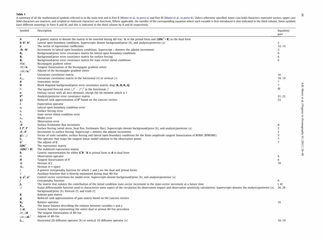
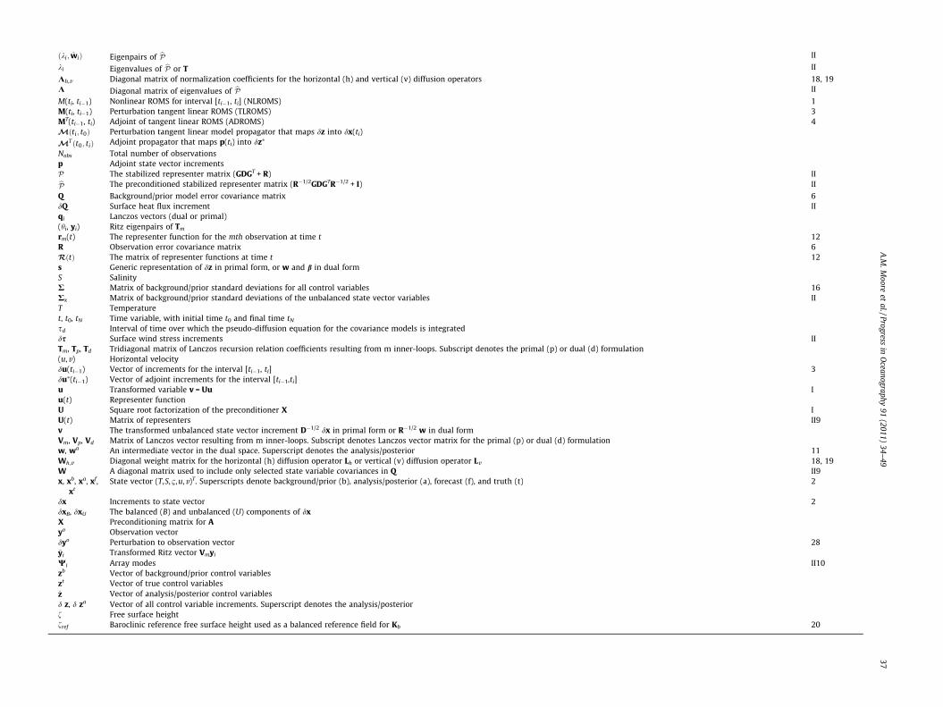
Table 1A summary of all the mathematical symbols referred to in the main text and in Part II (Moore et al., in press-a) and Part III (Moore et al., in press-b). Unless otherwise specified, lower case bold characters represent vectors, upper casebold characters are matrices, and scripted or italicized characters are functions. Where applicable, the number of the corresponding equation where each variable is first introduced is also indicated in the third column. Some symbolshave different meanings in Parts II and III, and this is indicated in the third column by II and III respectively.

Symbol Description Equation/part

A A generic matrix to denote the matrix to be inverted during 4D-Var; H in the primal form and (GDGT + R) in the dual formb, bb, ba Lateral open boundary conditions. Superscripts denote background/prior (b), and analysis/posterior (a) 2b The vector of representer coefficients 12, 13db, db⁄ Increments to lateral open boundary conditions. Superscript ⁄ denotes the adjoint increments 2Bb Background/prior error covariance matrix for lateral open boundary conditions 6Bf Background/prior error covariance matrix for surface forcing 6Bx Background/prior error covariance matrix for state vector initial conditions 6B(x) Biconjugate gradient solver@B=@x Tangent linearization of the biconjugate gradient solver

ð@B=@xÞT Adjoint of the biconjugate gradient solver

C Univariate correlation matrix 16Ch,v Univariate correlation matrix in the horizontal (h) or vertical (v) 18, 19d Innovation vector 7D Block diagonal background/prior error covariance matrix, diag (Bx,Bf,Bb,Q) 7es The squared forecast error ðJ f � J tÞ2 in the functional J III

ei Unitary vector with all zero elements, except the ith element which is 1Ea Analysis/posterior error covariance matrix 21, 22eEa Reduced rank approximation of Ea based on the Lanczos vectors 23

E Expectation operatoreb Lateral open boundary condition erroref Surface forcing errorei State vector initial condition errorem Model erroreo Observation errordF Surface freshwater flux increment IIf, fb, fa Surface forcing (wind stress, heat flux, freshwater flux). Superscripts denote background/prior (b), and analysis/posterior (a) 2df, df⁄ Increments to surface forcing. Superscript ⁄ denotes the adjoint increments 2g(ti�1) Vector of state variables, surface forcing and lateral open boundary conditions for the finite amplitude tangent linearization of ROMS (RPROMS) 5G The operator that maps the tangent linear model solution to the observation points 7GT The adjoint of G 7GDGT The representer matrix(GDGT + R) The stabilized representer matrixh Generic representation for either GTR�1d in primal form or d in dual formH Observation operator 6H Tangent linearization of H 6H Hessian of J 10Hv Hessian in v-spaceI A generic cost/penalty function for which I and J are the dual and primal formsI Auxiliary function that is directly minimized during dual 4D-Varg, gb, ga Control vector corrections for model error. Superscripts denote background/prior (b), and analysis/posterior (a)J Cost/penalty function 6J0 The matrix that isolates the contribution of the initial condition state-vector increment to the state-vector increment at a future time I, IIIJ Scalar differentiable function used to characterize some aspect of the circulation for observation impact and observation sensitivity calculations. Superscripts denotes the analysis/posterior (a),

background/prior (b), forecast (f), and truth (t)26, 28

K Kalman gain matrixeK Reduced rank approximation of gain matrix based on the Lanczos vectors

Kb Balance operator 16Kxy The linear balance describing the relation between variables x and yKðdÞ Generic function representing the entire dual or primal 4D-Var procedure@K=@d The tangent linearization of 4D-Var

ð@K=@dÞT Adjoint of 4D-Var

Lh,v Horizontal 2D diffusion operator (h) or vertical 1D diffusion operator (v) 18, 19

36A

.M.M

ooreet

al./Progressin

Oceanography

91(2011)

34–49

ðki; wiÞ Eigenpairs of bP II

ki Eigenvalues of bP or T II

Kh,v Diagonal matrix of normalization coefficients for the horizontal (h) and vertical (v) diffusion operators 18, 19K Diagonal matrix of eigenvalues of bP II

M(ti, ti�1) Nonlinear ROMS for interval [ti�1, ti] (NLROMS) 1M(ti, ti�1) Perturbation tangent linear ROMS (TLROMS) 3MT(ti�1, ti) Adjoint of tangent linear ROMS (ADROMS) 4Mðti; t0Þ Perturbation tangent linear model propagator that maps dz into dx(ti)MT ðt0; tiÞ Adjoint propagator that maps p(ti) into dz⁄

Nobs Total number of observationsp Adjoint state vector incrementsP The stabilized representer matrix (GDGT + R) IIbP The preconditioned stabilized representer matrix (R�1/2GDGTR�1/2 + I) II

Q Background/prior model error covariance matrix 6dQ Surface heat flux increment IIqi Lanczos vectors (dual or primal)(hi, yi) Ritz eigenpairs of Tm

rm(t) The representer function for the mth observation at time t 12R Observation error covariance matrix 6RðtÞ The matrix of representer functions at time t 12s Generic representation of dz in primal form, or w and b in dual formS SalinityR Matrix of background/prior standard deviations for all control variables 16Rx Matrix of background/prior standard deviations of the unbalanced state vector variables IIT Temperaturet, t0, tN Time variable, with initial time t0 and final time tN

sd Interval of time over which the pseudo-diffusion equation for the covariance models is integratedds Surface wind stress increments IITm, Tp, Td Tridiagonal matrix of Lanczos recursion relation coefficients resulting from m inner-loops. Subscript denotes the primal (p) or dual (d) formulation(u,v) Horizontal velocitydu(ti�1) Vector of increments for the interval [ti�1, ti] 3du⁄(ti�1) Vector of adjoint increments for the interval [ti�1,ti]u Transformed variable v = Uu Iu(t) Representer functionU Square root factorization of the preconditioner X IU(t) Matrix of representers II9v The transformed unbalanced state vector increment D�1/2 dx in primal form or R�1/2 w in dual formVm, Vp, Vd Matrix of Lanczos vector resulting from m inner-loops. Subscript denotes Lanczos vector matrix for the primal (p) or dual (d) formulationw, wa An intermediate vector in the dual space. Superscript denotes the analysis/posterior 11Wh,v Diagonal weight matrix for the horizontal (h) diffusion operator Lh or vertical (v) diffusion operator Lv 18, 19W A diagonal matrix used to include only selected state variable covariances in Q II9x, xb, xa, xf,

xtState vector (T,S,1,u,v)T. Superscripts denote background/prior (b), analysis/posterior (a), forecast (f), and truth (t) 2

dx Increments to state vector 2dxB, dxU The balanced (B) and unbalanced (U) components of dxX Preconditioning matrix for Ayo Observation vectordyo Perturbation to observation vector 28yi Transformed Ritz vector Vmyi

Wi Array modes II10zb Vector of background/prior control variableszt Vector of true control variablesz Vector of analysis/posterior control variablesd z, d za Vector of all control variable increments. Superscript denotes the analysis/posteriorf Free surface heightfref Baroclinic reference free surface height used as a balanced reference field for Kb 20

A.M

.Moore

etal./Progress

inO

ceanography91

(2011)34–

4937

38 A.M. Moore et al. / Progress in Oceanography 91 (2011) 34–49

referred to as TLROMS, and with initial conditions dx(t0), forcingdf(t) and open boundary conditions db(t).

An operator of central importance to 4D-Var is MT(ti�1, ti) thematrix transpose of the tangent linear model which is integratedbackwards, hence the order of the time arguments for MT is re-versed. The transpose of TLROMS represents the matrix adjointwith respect to the L2 inner-product, and is associated with the ad-joint equation:

du�ðti�1Þ ¼MTðti�1; tiÞpðtiÞ ð4Þ

where du�ðti�1Þ ¼ ðpTðti�1Þ; df�TðtiÞ; db�TðtiÞÞT with p being the ad-joint state-vector increment, and df⁄ and db⁄ the adjoint of the sur-face forcing and open boundary condition increments. Eq. (4) willhereafter be referred to as ADROMS, and integrations of ADROMSalways start with p(tN) = 0.

While the incremental approach to 4D-Var described later relieson NLROMS in (1) to propagate xb forward in time, the representermethod of Bennett (2002) employs a finite-amplitude linearizationof ROMS. Specifically, if xk denotes the kth member of a linear se-quence of k-iterates (identified later as ‘‘outer-loops’’), then:

xkðtiÞ ¼ Mðti; ti�1Þðxk�1ðti�1Þ; fk�1ðtiÞ;bk�1ðtiÞÞ þMk�1ðti; ti�1Þ� ðgkðti�1Þ � gk�1ðti�1ÞÞ ð5Þ

where Mk�1 is TLROMS linearized about xk�1 over the time interval[ti�1, ti]. Eq. (5) is linear in gk = (xk

T, fkT,bk

T)T, and represents the fi-nite-amplitude tangent linearization of ROMS, hereafter referredto as RPROMS. The linear sequence described by (5) is also com-monly referred to as Picard iterations (Bennett, 2002) and moregenerally is used to establish the existence of solutions of nonlineardifferential equations. If we denote (gk(ti�1) � gk�1(ti�1)) as dgk(ti�1),then the second term on the rhs of (5) is of the formMk�1(ti, ti�1)dgk(ti�1) which is mathematically equivalent to TLROMSin (3). RPROMS therefore differs from TLROMS by the addition of thefirst term on the rhs of (5) which represents the NLROMS operatorsapplied to the previous iterate gk�1. A detailed discussion of RPROMSis beyond the scope of this paper, although some additional informa-tion can be found in Di Lorenzo et al. (2007). The linearization em-ployed in RPROMS is not unique and there are several possiblechoices as discussed by Bennett (2002) where illustrative examplesare also presented. In the case of ROMS, RPROMS is constructed byadding to TLROMS the appropriate NLROMS terms computed fromgk�1.

TLROMS, ADROMS and RPROMS currently exist for all of thecommonly used numerical and physical options employed inROMS. Notable exceptions include most of the vertical mixingand turbulence closure schemes where some of the tangent linearterms must be excluded to prevent the growth of highly unstablemodes. The tangent linear and adjoint versions of the surface bulkflux formulations are also linearly unstable in many cases, so aregenerally not used. TLROMS and ADROMS are described in moredetail by Moore et al. (2004).

3. Incremental 4D-Var

The goal of 4D-Var is to identify the best estimate circulation,also commonly referred to as the analysis or posterior, namelyxa(t), that minimizes in a least-squares sense, the difference be-tween the model and the observations and a background, subjectto prior hypotheses about errors and possibly additional con-straints. The solution, x(ti), of NLROMS that describes xa will de-pend upon the choice of initial conditions, x(t0), surface forcing,f(t), and boundary conditions, b(t), all of which are subject to errorsand uncertainties. As such, x(t0), f(t) and b(t) are referred to as con-trol variables, and the problem in 4D-Var is reduced to identifyingthe appropriate combination of control variables that yield the best

estimate xa(t). In general, there will be other sources of error anduncertainty associated with the model dynamics and numerics,and unresolved scales of motion (see Daley (1991) and Cohn(1997) for in-depth discussions), which we collectively denote as�m(ti), and introduce an additional vector of control variables g(ti)on the rhs of (1) depending on the 4D-Var approach adopted. To ac-count for model errors, the vector of increments du in (3) is aug-mented so that du(ti�1) = (dx(ti�1)T, dfT(ti), dbT(ti), gT(ti))T, and thetangent linear operator M(ti, ti�1) also advances the correction formodel error forward in time, assuming a background correctiongb(ti) = 0. Similarly, the adjoint vector associated with (4) is givenby du�ðti�1Þ ¼ ðpTðti�1Þ; df�TðtiÞ; db�TðtiÞ;g�TðtiÞÞT .

The development of incremental 4D-Var presented here isbased on Courtier et al. (1994) and Courtier (1997), but in an ex-panded form in which the uncertainties in the surface forcingand lateral boundary conditions are explicitly identified followingDaget et al. (2009). The incremental approach to 4D-Var consistsof minimizing an objective function, J, given by:

Jðdxðt0Þ; dfðt1Þ; . . . ; dfðtkÞ; . . . ; dbðt1Þ; . . . ; dbðtkÞ; . . . ;gðt1Þ; . . . ;gðtkÞ; . . .Þ

¼ 12

dxTðt0ÞB�1x dxðt0Þ þ

12

XN

k¼1

XN

j¼1

dfTðtkÞB�1f ðtk; tjÞdfðtjÞ

n

þdbTðtkÞB�1b ðtk; tjÞdbðtjÞ þ gTðtkÞQ�1ðtk; tjÞgðtjÞ

oþ 1

2

Xn

i¼0

Xn

l¼0

ðHidxðtiÞ � diÞT R�1i;l ðHldxðtlÞ � dlÞ ð6Þ

where from (2) the increment dx(tk) = x(tk) � xb(tk), and ti and tl areidentified here as the n observation times. The innovation vectordi ¼ yo

i � HiðxbðtiÞÞ represents the difference between the vector ofobservations yo

i at time ti and the model analogue of the observa-tions computed from the background circulation xb(ti) accordingto the observation operator Hi. In general, Hi will be nonlinear andserves to transform the model state vector to observed variablesand to interpolate them to observation points in space and time. Er-rors arising from Hi are included in R Janjic and Cohn (2006), andthe operator Hi is the tangent linearization of Hi. While the se-quence of times tk and tj associated with the forcing, boundary con-ditions and model errors will, in general, correspond to each of theN model timesteps spanning the assimilation interval, in practice tk

and tj are typically evaluated less frequently than every timestep.If �i, �f(t), �b(t), �o and �m(t) denote errors in xb(t0), fb(t), bb(t), yo

and the model respectively, then implicit in (6) is the assumptionof random, unbiased errors so that E(�i) = 0, E(�f(t)) = 0,E(�b(t)) = 0, E(�m(t)) = 0 and E(�o) = 0, where E denotes the expecta-tion operator. The associated error covariances are denoted:E �i�T

i

� �¼ Bx, the initial condition background error covariance ma-

trix; Eð�f ðtkÞ�Tf ðtjÞÞ ¼ Bf ðtk; tjÞ, the surface forcing background error

covariance matrix; Eð�bðtkÞ�TbðtjÞÞ ¼ Bbðtk; tjÞ, the lateral boundary

condition background error covariance matrix; Eð�mðtkÞ�TmðtjÞÞ ¼

Q ðtk; tjÞ, the model error covariance matrix; and Eð�oðtiÞ�ToðtjÞÞ ¼

Ri;j, the observation error covariance matrix. In addition, it is as-sumed that the individual sources of error are uncorrelated, so thatE �i�T

f ðtkÞ� �

¼ 0, E �i�TbðtkÞ

� �¼ 0, E(�ig

T(tk)) = 0, E �i�ToðtkÞ

� �¼ 0,

E �f ðtjÞ�TbðtkÞ

� �¼ 0, etc. Finally, we assume no temporal autocorre-

lations, and time invariant background error covariances in whichcase Bf(tk, tj) = dk, jBf, Bb(tk, tj) = dk, jBb, Q(tk, tj) = dk, jQ, and Ri, l = di, lRi,and the double summations in (6) are replaced by a single summa-tion. These statements about the error statistics of the background,observations, forcing, boundary conditions and model represent aprecise statement about our prior hypotheses.

The objective function J in (6) is referred to as the cost function(or penalty function), and it is customary to write (6) in a morecompact form (Courtier, 1997) by introducing the vectordz = (dx(t0)T, dfT(t1), . . . ,dfT(tk), . . . ,bT(t1), . . . ,dbT(tk), . . . ,gT(t1), . . . ,gT(tk). . .)T which describes all of the control variable increments.

A.M. Moore et al. / Progress in Oceanography 91 (2011) 34–49 39

The increment vector dz differs from du(t) introduced earlier inthat dz is comprised of all the elements of the control vector, whiledu(t) describes only a subset of the control vector elements. Fur-thermore, the interpolated and/or transformed increments Hidx(ti)can be expressed as HiMðti; t0Þdz ¼ Gidz, where Mðti; t0Þ is analternative form of the tangent linear operator that isolates thestate vector increment as described in the appendix. Finally, we

introduce the following: the matrix G ¼ . . . ;GTi ; . . .

� �T; the vector

d ¼ . . . ;dTi ; . . .

� �Tof innovations of length Nobs; the block diagonal

matrix R with blocks Ri; and the block diagonal matrix D withblocks Bx, Bf, Bb and Q. The cost (penalty) function can then be writ-ten as:

JðdzÞ ¼ 12

dzT D�1dzþ 12ðGdz� dÞT R�1ðGdz� dÞ: ð7Þ

The desired analysis increment, dza, that minimizes (7) corre-sponds to the solution of the equation @J/@dz = 0, and is given by:

dza ¼ ðD�1 þ GT R�1GÞ�1GT R�1d ð8Þ¼ DGTðGDGT þ RÞ�1d: ð9Þ

Eq. (9) is algebraically equivalent to optimum interpolation (Lorenc,1986), and is referred to as the dual form, while (8) is some timesreferred to as the primal form. If the vector zb = (xbT, fb(t1)T, . . . ,fb(tk)T, . . . ,bb(t1)T, . . . ,bb(tk)T, . . . ,0T)T represents the background con-trol vector, then the best estimate of the circulation is given byz ¼ zb þ dza.

3.1. Strong versus weak constraint 4D-Var

It is common in 4D-Var to neglect errors in the model, in whichcase �m(tk) = 0. In addition, the assumption is often made that thesurface and lateral boundary conditions are error-free, in whichcase �f(tk) = 0 and �b(tk) = 0 also. Following Sasaki (1970), suchapplications of 4D-Var are subject to a ‘‘strong constraint’’ imposedby the model dynamics which amounts to neglecting the secondterm on the rhs of (6). In oceanographic applications, the term‘‘strong constraint’’ is also generally used when only model erroris neglected, and we will adopt this convention here. When modelerrors are admitted (�m(tk) – 0), 4D-Var is said to be subject to a‘‘weak constraint’’ imposed by the model dynamics. Additional re-cent discussions of the issues surrounding model error and weakconstraint 4D-Var can be found in Trémolet (2006, 2007).

3.2. Model space versus observation space

Consider Eq. (8) where identifying dza is equivalent to solvingthe linear equation Hdza ¼ GT R�1d where:

H ¼ ðD�1 þ GT R�1GÞ ð10Þ

is the Hessian of J. In practice, the estimate of dza is computed iter-atively by minimizing the cost (penalty) function in (7), which recallcorresponds to finding dz that satisfies @J/@dz = 0. According to (8),this is a very challenging problem because the dimension nz of dzis very large, especially in the case of weak constraint 4D-Var wherethe correction for model error g(tk) must be identified, in principle,for every model timestep. For this reason, Eq. (8) is usually em-ployed only for strong constraint 4D-Var, in which case the dimen-sion of dz is equal to the number of model gridpoint variables plusall the points in space and time that define the surface and lateralboundary conditions. Strong constraint 4D-Var using (8) thereforeinvolves a search for the optimal circulation estimate in the spacespanned by the model control vector.

3.2.1. Incremental strong constraint 4D-Var (I4D-Var)It is important to realize that while (8) is written in terms of a

series of matrix operations, the matrices are never explicitly com-puted. Instead, matrix–vector products are evaluated using theappropriate model components, including the covariance matricesthat are modeled as solutions of diffusion equations as discussed inSection 5. Thus the solution of (8) can be expressed as an iterativesequence of matrixless operations as illustrated in Fig. 1 (see alsoCourtier, 1997). The solution of (8) proceeds by solving an equiva-lent system of linear equations using a preconditioned Lanczos for-mulation of the conjugate gradient method, and the steps in Fig. 1associated with the ‘‘Lanczos algorithm’’ and ‘‘preconditioner’’ aredescribed in Sections 4 and 5. Steps (ii)–(vi) in Fig. 1 are referredto as an inner-loop, and when repeated represent the minimizationof J in the space spanned by the control vector in the vicinity of zb.

To account for nonlinearities, it is often advantageous to also re-fine the nonlinear model solution about which TLROMS and ADR-OMS are initialized. In this case, then using (2), step (vii) of Fig. 1is performed with the new initial condition xk(t0) = xb(t0) + dxk(t0),fk(t) = fb(t) + dfk(t) and bk(t) = bb(t) + dbk(t), where k refers to thenew run of NLROMS, and dxk(t0), dfk(t) and dbk(t) are the incre-ments computed during step (vi) of the previous inner-loop. Step(vii) is referred to as an outer-loop, and TLROMS and ADROMSare linearized about xk during the next sequence of inner-loops.A subscript k is therefore also implied for G and GT but has beenomitted for the sake of clarity. It is also important to note thatthe innovation vector d is always computed relative to the back-ground circulation xb(t) and is not updated between outer-loops.This aspect of 4D-Var in ROMS follows Bennett (2002) and differsfrom the practice followed in some other models where d is some-times updated between outer-loops.

3.2.2. A physical-space statistical analysis system (4D-PSAS)The best estimate increment dza is also given by the dual form

(9), which can be written equivalently as dza = DGTwa where wa

is a vector in the dual of x and satisfies:

ðGDGT þ RÞwa ¼ d: ð11Þ

The dual form has the advantage that the dimension of wa is equalto the number of observations which, in oceanographic applica-tions, is typically several orders of magnitude smaller than thedimension of the control vector. Therefore, solving (11) may befar less challenging than solving (8). Once wa has been identified,dza = DGTwa can be computed by a single integration of ADROMS,GT, followed by a multiplication by the error covariance matrix D.

More importantly, however, the dimension of wa is indepen-dent of the strong and weak constraint; despite the enormous dif-ference in the dimension of dza when comparing the strong andweak constraint case, wa always has the dimension of the numberof observations. The dual form (9) therefore involves a search forthe best circulation estimate in the space of linear functions (i.e.G) of the state vector dx spanned only by the observations, whichmakes the weak constraint estimation problem more tractable.

Since (8) and (9) are equivalent, the primal and dual formula-tions yield identical solutions dza. Courtier (1997) notes thatthe solution of (11) minimizes the function IðwÞ ¼ 1

2 wT

ðGDGT þ RÞw�wT d which is equivalent to the physical-space sta-tistical analysis system (PSAS) proposed by Da Silva et al. (1995).The solution of (9) via (11) (i.e. by minimizing of Iðw)) in the pres-ence of either the weak or strong constraint proceeds iteratively asshown in Fig. 2. Repeated application of the inner-loops (steps (ii)–(vi)), followed by steps (vii) and (viii) is equivalent to minimizationof J but now in observation space. Analogous to I4D-Var, the ‘‘out-er-loop’’ step (ix) may be repeated to update the circulation aboutwhich TLROMS and ADROMS are linearized, but d is alwayscomputed relative to the background xb(t).

Fig. 1. A flow chart illustrating the strong constraint ROMS I4D-Var algorithm. The individual model components NLROMS, TLROMS and ADROMS are all identified, and theArabic numbers in parentheses refer to the appropriate equation numbers in the main text. The Roman numerals refer to the different components of the inner- and outer-loops described in Section 3.2.1. The calling sequence of the sub-algorithms for the covariance model, Lanczos algorithm and preconditioner in relation to the integration ofeach model component is also indicated, and § indicates the section number in the main text where each sub-algorithm is described. The arrows to the left (right) of the boxesdenote inputs (outputs) associated with the individual model components. The integer m (k) refers to the number of inner- (outer-) loops, and all symbols are defined in themain text and Table 1.

40 A.M. Moore et al. / Progress in Oceanography 91 (2011) 34–49

3.2.3. The method of representers (R4D-Var)Bennett (1992) describes an alternative approach to dual 4D-

Var where the best estimate state-vector xa is expressed as:

xaðtÞ ¼ xbðtÞ þ RðtÞb ð12Þ

where each column of the matrix RðtÞ is a representer function de-noted rm(t), with one representer function associated with each ofthe m = 1, . . . ,Nobs observations, and b is the (Nobs � 1) vector ofrepresenter coefficients. If ~xðtÞ denotes the response of the modelto random forcing with statistics that are consistent with the priorhypotheses of Section 3, then each representer rm(t) describes thecovariance between the circulation ~xðtÞ sampled at the space–timelocation of the mth observation and the field ~xðtÞ at all other pointsand times (Bennett, 2002, Sections 2.2 and 2.4).

Computation of each column of R requires one integration ofADROMS and one integration of TLROMS, so if Nobs is large, it isnot practical to compute all of the representers explicitly. How-ever, Eq. (12) indicates that all that is required is the productRðtÞb which can be cleverly evaluated using the indirect repre-senter method introduced by Egbert et al. (1994). The vector ofrepresenter coefficients, b, is in fact the solution of:

ðGDGT þ RÞb ¼ d ð13Þ

(Chua and Bennett, 2001), where (13) is analogous to (11). Theprocedure for solving (13) subject to either the strong or weak con-straint is illustrated in Fig. 3, and is similar to that used for 4D-PSASexcept now x(t) about which TLROMS and ADROMS are linearized is

computed using RPROMS. Fig. 3 shows that RPROMS is run at step(ii) and step (x) which mark the start and end of each outer-loop,k. The RPROMS solution at step (ii) is always obtained using thebackground initial condition, xb(t0), surface forcing, fb(t), andboundary conditions, bb(t). Therefore during the first outer-loop(k = 1) the RPROMS solution at step (ii) and the NLROMS solutionxðtÞ at step (i) (about which step (ii) is linearized when k = 1) areidentical, in which case (11) and (13) are equivalent and 4D-PSASand R4D-Var yield the same inner-loop solutions. Therefore duringthe first outer-loop, step (ii) is redundant, but is included in Fig. 3for completeness. Conversely, at step (x) in Fig. 3 the incrementscomputed at the end of the last inner-loop are applied to RPROMS,which yields a new outer-loop circulation estimate xk(t) accordingto (5). It is at this point that solutions of R4D-Var and 4D-PSAS di-verge. During outer-loops k > 1, RPROMS at steps (ii) and (x) is lin-earized about the circulation xkðtÞ ¼ xbðtÞ þ dxkðtÞ identified at theend of the previous inner-loop, and forced by fk(t) = fb(t) + dfk(t)and subject to bk(t) = bb(t) + dbk(t).

The matrix GDGT is referred to as the representer matrix and isthe covariance between the model fields sampled at each observa-tion space–time location. For closely spaces observations, such assatellite data, GDGT may be poorly conditioned in which case theaddition of the observation error covariance matrix R improvesthe conditioning of (13), and (GDGT + R) is called the stabilizedrepresenter matrix.

As discussed by Bennett (1992, 2002), the best circulation esti-mate xa(t) given by (12) satisfies the nonlinear Euler–Lagrangeequations, and the R4D-Var algorithm summarized above

Fig. 2. A flow chart illustrating the ROMS 4D-PSAS algorithm. The individual model components NLROMS, TLROMS and ADROMS are all identified, and the Arabic numbers inparentheses refer to the appropriate equation numbers in the main text. The Roman numerals refer to the different components of the inner- and outer-loops described inSection 3.2.2. The calling sequence of the sub-algorithms for the covariance model, Lanczos algorithm and preconditioner in relation to the integration of each modelcomponent is also indicated, and § indicates the section number in the main text where each sub-algorithm is described. The arrows to the left (right) of the boxes denoteinputs (outputs) associated with the individual model components. The integer m (k) refers to the number of inner- (outer-) loops, and all symbols are defined in the maintext and Table 1.

A.M. Moore et al. / Progress in Oceanography 91 (2011) 34–49 41

represents a linear iterative approach for solving the nonlinearEuler–Lagrange equations for ROMS. The outer-loops of R4D-Varare based on Picard iterates, commonly used to establish the exis-tence of a solution to a nonlinear differential equation (Gesztesyand Sticka, 1998), and it is in this sense that R4D-Var fundamen-tally differs from 4D-PSAS of Section 3.2.2. During R4D-Var, boththe inner- and outer-loops are linear, and during the outer-loopsdynamical information is conveyed using RPROMS. As discussedin detail by Bennett (2002), a complete linearization of the problemis essential for identifying the true optimal circulation estimate.This is in contrast to 4D-PSAS where NLROMS is used in the out-er-loops, in which case a suboptimal estimate will result.

4. Conjugate gradients and the Lanczos Algorithm

Identification of the best circulation estimate using either I4D-Var, 4D-PSAS or R4D-Var involves the solution of a sequence of lin-ear least-squares minimizations. Each 4D-Var algorithm attemptsto solve a linear equation by minimizing the cost (penalty) func-tional J in (7). In I4D-Var J is minimized directly in the full spacespanned by the control vector, while in 4D-PSAS and R4D-Varthe minimum of J is identified indirectly by minimizing an auxill-iary function I (via (11) or (13)) in observation space. Both J andI can be written in a generic quadratic form as IðsÞ ¼12 sT As� sT hþ c. The minimum of I corresponds to the condition

@I/@s = 0 for which s satisfies the linear equation As = h. For I4D-Var, inspection of (7) shows that s = dz, h = GTR�1d, c ¼ 1

2 dT R�1d,and A ¼H ¼ ðD�1 þ GT R�1GÞ the Hessian of J given by (10). Eqs.(11) and (13) show that for 4D-PSAS and R4D-Var, s is equivalentto the intermediate solution in observation space given by w andb respectively, and in both cases c = 0, h = d and A = (GDGT + R),the stabilized representer matrix.

In ROMS, a conjugate gradient descent method recast in theform of a Lanczos algorithm is employed to solve As = h in all threecases (Fisher and Courtier, 1995). The close connection betweenthe conjugate gradient descent method and the Lanczos algorithmwas first made by Paige and Saunders (1975) and is discussed atlength by Golub and van Loan (1989). The Lanczos algorithm is fa-vored here because it offers tremendous additional utility to ROMS4D-Var, as described in Section 7 and the companion papers Mooreet al. (in press-a), Moore et al. (in press-b).

Following Lanczos (1950), a reduced rank factorization of thesymmetric, positive definite matrix A can be found which satisfiesthe recurrence relation given by:

AVm ¼ VmTm þ cmqmþ1eTm ð14Þ

where Vm = (. . .,qi, . . .), i = 1, . . . ,m, is a matrix composed of theorthonormal vectors qi, referred to as the Lanczos vectors. Thematrix T is a (m �m) symmetric tridiagonal matrix with leadingdiagonal elements di, i = 1, . . . ,m, and off-diagonal elements ci,

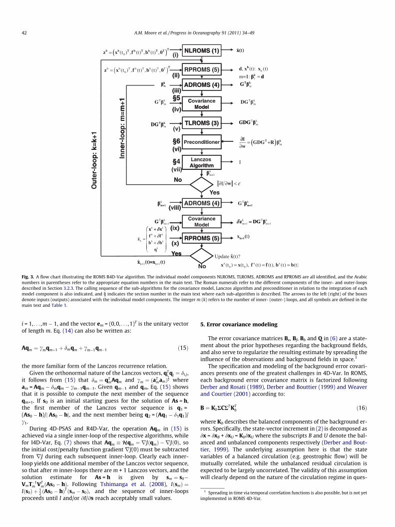
Fig. 3. A flow chart illustrating the ROMS R4D-Var algorithm. The individual model components NLROMS, TLROMS, ADROMS and RPROMS are all identified, and the Arabicnumbers in parentheses refer to the appropriate equation numbers in the main text. The Roman numerals refer to the different components of the inner- and outer-loopsdescribed in Section 3.2.3. The calling sequence of the sub-algorithms for the covariance model, Lanczos algorithm and preconditioner in relation to the integration of eachmodel component is also indicated, and § indicates the section number in the main text where each sub-algorithm is described. The arrows to the left (right) of the boxesdenote inputs (outputs) associated with the individual model components. The integer m (k) refers to the number of inner- (outer-) loops, and all symbols are defined in themain text and Table 1.

42 A.M. Moore et al. / Progress in Oceanography 91 (2011) 34–49

i = 1, . . . ,m � 1, and the vector em = (0,0, . . . ,1)T is the unitary vectorof length m. Eq. (14) can also be written as:

Aqm ¼ cmqmþ1 þ dmqm þ cm�1qm�1 ð15Þ

1 Spreading in time via temporal correlation functions is also possible, but is not yetplemented in ROMS 4D-Var.

the more familiar form of the Lanczos recurrence relation.Given the orthonormal nature of the Lanczos vectors, qT

i qj ¼ di;j,it follows from (15) that dm ¼ qT

mAqm and cm ¼ ðaTmamÞ

12 where

am = Aqm � dmqm � cm�1qm�1. Given qm�1 and qm, Eq. (15) showsthat it is possible to compute the next member of the sequenceqm+1. If s0 is an initial starting guess for the solution of As = h,the first member of the Lanczos vector sequence is q1 =(As0 � h)/j As0 � hj, and the next member being q2 = (Aq1 � d1q1)/c1.

During 4D-PSAS and R4D-Var, the operation Aqm in (15) isachieved via a single inner-loop of the respective algorithms, whilefor I4D-Var, Eq. (7) shows that Aqm �Hqm ¼ rJðqmÞ � rJð0Þ, sothe initial cost/penalty function gradient rJ(0) must be subtractedfrom rJ during each subsequent inner-loop. Clearly each inner-loop yields one additional member of the Lanczos vector sequence,so that after m inner-loops there are m + 1 Lanczos vectors, and thesolution estimate for As = h is given by sm ¼ s0�VmT�1

m VTmðAs0 � hÞ. Following Tshimanga et al. (2008), IðsmÞ ¼

Iðs0Þ þ 12 ðAs0 � hÞTðsm � s0Þ, and the sequence of inner-loops

proceeds until I and/or @I/@s reach acceptably small values.

5. Error covariance modeling

The error covariance matrices Bx, Bf, Bb and Q in (6) are a state-ment about the prior hypotheses regarding the background fields,and also serve to regularize the resulting estimate by spreading theinfluence of the observations and background fields in space.1

The specification and modeling of the background error covari-ances presents one of the greatest challenges in 4D-Var. In ROMS,each background error covariance matrix is factorized followingDerber and Rosati (1989), Derber and Bouttier (1999) and Weaverand Courtier (2001) according to:

B ¼ KbRCRT KTb ð16Þ

where Kb describes the balanced components of the background er-rors. Specifically, the state-vector increment in (2) is decomposed asdx = dxB + dxU = KbdxU where the subscripts B and U denote the bal-anced and unbalanced components respectively (Derber and Bout-tier, 1999). The underlying assumption here is that the statevariables of a balanced circulation (e.g. geostrophic flow) will bemutually correlated, while the unbalanced residual circulation isexpected to be largely uncorrelated. The validity of this assumptionwill clearly depend on the nature of the circulation regime in ques-

im

A.M. Moore et al. / Progress in Oceanography 91 (2011) 34–49 43

tion, but experience shows that it is a useful approximation forpractical purposes. The balance operator Kb in (16) is therefore de-fined so that the unbalanced components dxU are approximatelymutually uncorrelated, in which case the correlation matrix C ofthe unbalanced component of the errors in (16) is block diagonal,univariate, with standard deviations given by the diagonal matrixR.

At scales of the ocean mesoscale and larger, the dominantdynamical balances for the circulation initial condition increments,dx(t0) = x(t0) � xb(t0), are geostrophic balance and hydrostatic bal-ance, while the properties of characteristic water masses provideuseful correlations between T and S (Ricci et al., 2005; Weaveret al., 2005). This information can be used to construct informativebalance operators Kb for the initial condition background errorcovariance matrix Bx. From (2), similar balance requirements canbe imposed on the increments db(t) = b(t) � bb(t) described by Bb

at open boundaries since the open boundary conditions are typi-cally derived from another model calculation in a larger model do-main. Surface forcing is usually derived from operationalatmospheric forecast model products for which estimates of theanalysis error may be available, and such information may proveuseful for characterizing the error statistics of surface forcingincrements, df(t) = f(t) � fb(t), described by Bf. Similarly, the domi-nant dynamical balances of the generally stable atmospheric mar-ine boundary layers that control the fluxes of momentum, heat,and freshwater across the air-sea interface can also be used as pro-cess model priors for the Kb component of Bf. In the current ROMS4D-Var systems, we account only for the balance constraints on theinitial condition and model error increments.

Various approaches for modeling error covariance matrices aredocumented in the scientific literature, and each has associatedadvantages and drawbacks. The method used in ROMS followsthe diffusion operator approach of Weaver and Courtier (2001)and is summarized next, although there is nothing to precludethe use of alternative approaches in the future.

5.1. The background error correlations, C

It is well known that the action of a correlation matrix C on avector x can be expressed as the solution of a diffusion equation(see Egbert et al. (1994), Weaver and Courtier (2001), and Bennett(2002), p. 64, for a detailed treatment). Specifically, consider thetwo-dimensional diffusion equation for a scalar quantity h:

@h=@s ¼ jr2h ð17Þ

where j is a spatially invariant diffusion coefficient, and r2 is theLaplacian operator in Cartesian coordinates. If (17) is discretizedon the model grid, and the grid point values arranged as a vectorh, solutions of (17) over the interval s = [0,sd] can be representedas hðsÞ ¼ ð4pjsÞ�

12Chð0Þ, where the correlation matrix C is associ-

ated with a time invariant, isotropic, homogeneous, Gaussian corre-lation function, with a squared correlation length scale L2 = 2jsd.The initial conditions h(0) are the field on which the correlation ma-trix operates, appropriately scaled to preserve the properties of acorrelation function (see below). Generalizations of the solution of(17) on a sphere are considered by Weaver and Courtier (2001)who show that L2 � 2jsd still holds to good approximation.

In three dimensions, it is usual to factorize the correlation ma-trix so that C = ChCv assuming that the horizontal (Ch) and vertical(Cv) correlation matrices are separable. This is typically done forcomputational convenience although there is no overwhelmingevidence to suggest that the correlations of the real ocean are sep-arable. Nonetheless, Cv can be modeled in the same way as Ch bysolving a 1-dimensional diffusion equation. In the case of the openboundary conditions for ROMS, the horizontal correlation of the

background error covariance matrix Bb is replaced by a 1D correla-tion along the boundary. If time dependence of the correlationmatrices in (6) is treated as separable from the spatial correlations,it can be modeled as an autoregression process (Bennett, 2002, p.65). However, as noted earlier, time dependent correlations arenot yet a part of ROMS 4D-Var.

Eqs. (6) and (7) for the cost (penalty) function suggest that theinverse covariance matrices are required. However, in practice thisis usually not the case; in the space of the control vector the needto invert D is circumvented by a transformation of variable (seeSection 6.1), while in observation space the best estimate givenby (9) involves the solution of a linear equation involving D notits inverse (see Section 4).

The practical implementation of (17) is somewhat involved be-cause of the grid dependence of the calculation. Since the modelgrid spacing is usually not uniform in the horizontal and vertical,it is necessary to account for variations in the grid cell dimensionswhen modeling Ch and Cv in order to preserve the properties of acorrelation function. In practice, Ch and Cv are further factorizedfollowing Weaver and Courtier (2001) so that:

Ch ¼ KhL12hW�1

h L12h

� �TKh ¼ C

12h C

12h

� �Tð18Þ

Cv ¼ KvL12vW�1

v L12v

� �TKv ¼ C

12v C

12v

� �Tð19Þ

where W is a diagonal matrix with elements corresponding to thegrid box areas in the case of Wh and level thicknesses in the caseof Wv; L represents the action of the matrix obtained by solvingeither a 1D (for Lv) or 2D (for Lh) diffusion equation; and K is a diag-onal matrix of normalization coefficients required to ensure that therange of Ch and Cv is ±1. A square root factorization is used in (18)and (19) to ensure that Ch and Cv remain symmetric in the presenceof the inevitable rounding errors that occur during each operation,and the square roots are achieved by integrating (17) over the inter-val s = [0,sd/2].

The most costly part of covariance modeling is the evaluation ofthe normalization factors K. However, if the horizontal and verticalcorrelation lengths do not change from one assimilation cycle tothe next, K need only be computed once. Determination of the ex-act normalization factors is generally computationally demandingbut possible, and in ROMS the elements of K can also be estimatedusing the randomization method introduced by Fisher and Courtier(1995).

At the present time, ROMS 4D-Var supports only homogeneous,isotropic correlation functions. However, these assumptions can berelaxed by replacing jr2h in (17) with a diffusion tensor formula-tion and a coordinate rotation as demonstrated by Weaver andCourtier (2001). This option will be available in a future releaseof ROMS 4D-Var. An alternative approach based on the Kroneckerproduct is discussed in Li et al. (2008).

5.2. The linear balance operator Kb

In ROMS, the set of linear balance relationships relating the bal-anced (dxB) and unbalanced (dxU) components of the analysisincrements dxa parallel those described by Weaver et al. (2005).Because of the controlling influence of temperature on the oceancirculation via density over much of the ocean (except perhaps atthe low temperatures of the deep ocean or high latitudes), all ofthe balance relations between the variables are based on dT, thetemperature increment, and, after all, temperature observationsare typically the most abundant observation type in the ocean.For practical purposes, the resulting balance operator Kb is a lowerblock triangular matrix which has the advantage that it is easy toinvert. Recalling that dx = (dT,dS,df,du,dv)T, Weaver et al. (2005)show that the linear balance equations can be written as:

44 A.M. Moore et al. / Progress in Oceanography 91 (2011) 34–49

dTk ¼ dTk

dSk ¼ Kk�1ST dTk þ dSU

dfk ¼ KfTdTk þ KfSdSk þ dfU

duk ¼ KuTdTk þ KuSdSk þ Kufdfk þ duU

dvk ¼ KvTdTk þ KvSdSk þ Kvfdfk þ dvU

where k refers to the number of the outer-loops, and Kxy representsthe linear balance relation between variable x and y. The balanceKk�1

ST is based on the water mass properties of the ocean statexb + dxk�1 of the previous outer-loop, while KfT and KfS are derivedfrom the density anomalies computed from the linearized equationof state dqk = �ak�1dTk + bk�1dSk. Refinements of this approach arediscussed by Haines et al. (2006) and Balmaseda et al. (2008).

Following Weaver et al. (2005), it is assumed that the balancedand unbalanced components of f correspond to the baroclinic andbarotropic components of the circulation respectively. The baro-clinic contribution to the free surface height, (denoted fref), duringouter-loop k satisfies:

r � Hrfref ¼ �r �Z 0

�H

Z 0

zrqkðz0Þ=q0dz0dz

�r �Z 0

�Hðuk � rukiþ uk � rvkjÞdzþr �

Z 0

�HFkdz

ð20Þ

where u is the velocity vector, i and j are unit vectors in the zonaland meridional directions, F represents the net influence of forcingand dissipation, and H is the ocean depth (Fukumori et al., 1998).The field fref is computed in ROMS using a biconjugate gradient(BCG) method to solve (20), and can be expressed as fref ¼ Bðxk

UÞ,where B describes the BCG procedure. The function B is nonlinearsince it involves dot-products of the BCG vectors, and because thesecond term on the rhs of (20) is nonlinear. According to theassumptions of the incremental approach to 4D-Var, the balancedincrements dfB� fref, where dfB ’ ð@BðxÞ=@xjxk

BÞdx and @BðxÞ=@xjxk

Bdenotes the tangent linearization of the BCG algorithm and solvesa tangent linear form of (20). The current default in ROMS 4D-Varis to retain only the first term on the rhs of (20), and this is the casefor the experiments presented in the companion papers Moore et al.(in press-a, in press-b). However in general, the other terms may beretained in the tangent linearization @BðxÞ=@xjxk

Bat the discretion of

the user, depending on the importance of the contributions of eachterm on the rhs of (20).

The balance relations KxT, KxS and Kxf for x = u and x = v are com-puted based on the assumption of geostrophic balance, while@BðxÞ=@x describes any ageostrophic contributions that may beimportant to the balance. According to (16), the transpose of thebalance operator is required when computing the action of B onthe model state-vector, so the adjoint of the BCG algorithm,ð@BðxÞ=@xÞT jxk

B, is also used.

6. Preconditioning

As described in Section 4, the primal and dual forms of 4D-Varare equivalent to minimizing a function of the formIðsÞ ¼ 1

2 sT As� sT hþ c. For I4D-Var, I is the cost (penalty) function(7), while for 4D-PSAS and R4D-Var, I is an auxiliary function. Ineither case, A is a symmetric, positive-definite matrix with orthog-onal eigenvectors that represent linearly independent directions inthe space defined by A. In both control space or observation space,I(s) represents a parabola with an aspect ratio determined by theeigenvalues of A. If the eigenvalues are widely separated, thenI(s) will be characterized by a parabola that is steep-sided in somedirections, and gently sloping in others. In this situation, A is con-

sidered to be poorly conditioned, and the conjugate gradient algo-rithm will generally converge rapidly in the directions associatedwith the largest eigenvalues of A, and slowly in other directions,particularly if the largest and smallest eigenvalues differ by manyorders of magnitude.

If A is an (N � N) matrix then the conjugate gradient algorithm isguaranteed with exact arithmetic to converge to the minimum of I inat most N iterations (Golub and van Loan, 1989). The goal of precon-ditioning is to achieve convergence in�N iterations, which can befacilitated by transforming A into a new matrix XTA that yields thesame minimum solution for I but has clustered eigenvalues and asmaller condition number (i.e. the ratio of the largest to the smallesteigenvalues of XTA). In this case the aspect ratio of the parabolic sur-face I is very similar in many or all directions. The preconditioningmatrix X is symmetric, positive-definite and can be factorized asX = UUT, where U is usually referred to as the square-root precondi-tioner. As noted in Section 4, identifying the minimum of I(s) corre-sponds to solving the linear system As = h, so by defining the changeof variable s ¼ Us, the preconditioned system can be written asUT AUs ¼ UT h. It is beyond the scope of this paper to discuss the re-quired properties of preconditioners, but there are many excellenttreatises on the subject (e.g. Golub and van Loan, 1989; Benzi,2002; Tshimanga, 2007; Tshimanga et al., 2008).

6.1. First-level preconditioning

In 4D-Var, it is customary to apply two levels of preconditioningwhen minimizing I(s). In the case of I4D-Var, I(s) � J(dz) given by(7), and A is the Hessian matrix, H, of J. A beneficial first-level ofpreconditioning is a transformation of variable v ¼ D�

12dxU via

the prior error covariance matrix (Lorenc, 2003), where dxU arethe unbalanced components of the increment (Weaver et al.,2005), which are assumed to be mutually uncorrelated. With thistransformation all of the transformed variables are then of thesame order, and the Hessian in v-space becomes Hv ¼ðIþ D

12GT R�1GD

12Þ. Clearly, the lower bound for eigenvalues of Hv

is 1, and if the number of observations Nobs is small compared tothe dimension of Hv (the usual case in oceanographic applica-tions), the eigenvalues will be clustered around 1, and the first-le-vel preconditioner U ¼ D�

12 possesses the desired quality. In

general, it is necessary to evaluate the action of both U and U�1

on a vector. However, as shown by Courtier et al. (1994), ifdx � v = 0 is chosen as the starting guess for each outer-loop ofI4D-Var, then only the action of U�1 ¼ D

12 on the state-vector is re-

quired and can be readily computed using the methods describedin Section 5.

For 4D-PSAS and R4D-Var, A � (GDGT + R), and the first-levelpreconditioner is chosen according to the change of variable

v ¼ R12w (Courtier, 1997) which transforms the problem into one

of solving R�12GDGT R�

12 þ I

� �v ¼ R�

12d with a lower bound of 1 for

the eigenvalues.

6.2. Second-level preconditioning

The convergence of the conjugate gradient algorithm to theminimum of I(s) may be further accelerated by a second level ofpreconditioning applied to v. Two second-level preconditionersare available in ROMS: the first is based on estimates of the eigen-vectors of A and follows Fisher and Courtier (1995), and the secondis based on the Ritz vectors of A and parallels Tshimanga et al.(2008). Tshimanga (2007) refers to these approaches as ‘‘spectral’’preconditioning and ‘‘Ritz’’ preconditioning respectively, and weadopt the same nomenclature here.

Estimates of the eigenvectors and Ritz vectors of A can be com-puted with little extra computational effort during execution of the

A.M. Moore et al. / Progress in Oceanography 91 (2011) 34–49 45

Lanczos algorithm described in Section 4 (Golub and van Loan,1989). Consider the eigenpairs (hi,yi) of the tridiagonal matrix Tm

in (14) after m inner-loops of either I4D-Var, 4D-PSAS or R4D-Var. Post-multiplying (14) by the eigenvector yi shows that:

Ayi ¼ hiyi þ cmqmþ1 eTmyi

� �where yi ¼ Vmyi. Clearly, ðhi; yiÞ are good approximations of theeigenpairs of A when li ¼ kcmqmþ1ðeT

myiÞk is small, and as m ap-proaches the dimension of A, then li ? 0 and the eigenpairs ðhi; yiÞare exact.

The approximate Hessian eigenpairs (hi,yi) are also referred toas Ritz pairs, and Fisher and Courtier (1995) show how they canbe used as effective second-level preconditioners during 4D-Var.Following the nomenclature and notation of Tshimanga (2007)and Tshimanga et al. (2008), spectral preconditioning is achievedby a change of variable v = Uu, where:

Uj ¼Ymi¼1

I� 1� hji

� �12

� �yj

i yji

� �T� �

U�1j ¼

Y1

i¼m

I� 1� hji

� ��12

� �yj

i yji

� �T� �

Here hji; y

ji

� �are the Ritz pairs that arise from each sequence of in-

ner-loops i = 1, . . . ,m during outer-loop j. Therefore, each outer-loopyields a new second-level preconditioner Uj that can be used to pre-condition subsequent outer-loops, and the resulting sequence ofpreconditioners Uj, j = 1,2, . . . ,k � 1 is applied sequentially duringouter-loop k via the change of variable vk ¼

Qk�1j¼1 Ujuk. However,

as Tshimanga et al. (2008) demonstrate, spectral preconditioningis only effective if li is sufficiently small. In practice, only those Ritzvectors for which �i ¼ Ayj

i � hjiy

ji

��� ���=hj1 ¼ li=h

j1 is sufficiently small

should be used, otherwise the second-level preconditioner mayactually degrade the convergence of the inner-loops.2

As an alternative, Tshimanga et al. (2008) propose Ritz precon-ditioning for which the error li associated with each yj

i is formallyincluded in Uj. Following Tshimanga (2007), the associated changeof variable vk ¼

Qk�1j¼1 Ujuk is given by:

Uj ¼Ymi¼1

I� 1� hji

� �12

� �yj

i yji

� �Tþ hj

i

� ��12

eTmyj

i

� �cmyj

iqTmþ1

� �

U�1j ¼

Y1

i¼m

I� 1� hji

� ��12

� �yj

i yji

� �T� hj

i

� ��1eT

myji

� �cmyj

iqTmþ1

� �

Tshimanga et al. (2008) demonstrate that Ritz preconditioning isless restrictive and more forgiving than spectral preconditioning be-cause even using relatively inaccurate Ritz vectors, as measured by�i, can lead to a significant reduction in the number of inner-loopsrequired to reduce I(s) to a given level.2

7. Tools for 4D-Var post-processing

A number of very useful tools are available for post-processingthe output of ROMS 4D-Var. These include estimates of the analysis(posterior) error variance, empirical orthogonal functions (EOFs) ofthe posterior error covariance matrix, and the adjoint of the entire4D-PSAS and R4D-Var system for computing the impact of obser-vations on the analysis-forecast system as well as the sensitivityto variations in the observations.

2 The same is true in ROMS as described at http://myroms.org/wiki/index.php/Variational_Data_Assimilation.

7.1. Analysis error estimates

If we denote by zt the vector describing the true state vector,surface forcing, and boundary conditions, then the analysis errorcovariance matrix is given by Ea = E((zb + dza � zt)(zb + dza � zt)T).Proceeding from (8), Ea can be expressed as:

Ea ¼ ðD�1 þ GT R�1GÞ�1 ð21Þ

which is the inverse of the Hessian of the cost (penalty) function gi-ven by (10). Alternatively, proceeding from the dual form (9), theanalysis error covariance can be written as:

Ea ¼ ðI� KGÞDðI� KGÞT þ KRKT ð22Þ

where K = DGT(GDGT + R)�1 is the Kalman gain matrix.The dimension of Ea is very large and it is computationally pro-

hibitive to calculate and save the full matrix. However, the Lanczosvector expansions of the Hessian in (10) and the stabilized repre-senter matrix in (9) can be used to compute a reduced rankapproximation to Ea. According to Section 4, a reduced rankapproximation eEa of Ea in (21) resultng from the primal formula-tion can be expressed as:

eEaM ¼ D

12VpT�1

p VTp D

12

� �Tð23Þ

where Vp is the matrix of primal Lanczos vectors of the Hessian H

resulting from a single outer-loop and M preconditioned inner-loops of I4D-Var, and Tp is the associated M �M tridiagonal matrix.Alternatively, using (22) and the dual formulation:

eEaM ¼ ðI� eKGÞD ð24Þ

¼ I� DGT R�12VdT�1

d VTd R�

12

� �TG

� �D ð25Þ

where eK ¼ DGT R�12VdT�1

d VTd R�

12

� �T, hereafter referred to as the prac-

tical gain matrix, is an approximation of the true gain matrix K; Vd

is the matrix of dual Lanczos vectors of the stabilized representermatrix resulting from a single outer-loop and M preconditioned in-ner-loops of 4D-PSAS or R4D-Var, and Td is the associated M �Mtridiagonal matrix. Eq. (24) is simpler than the Joseph form (22) be-cause the space spanned by the uncomputed Lanczos vectors in thesequence (14) for m > M is orthogonal to the space spanned by Vd. Ifthe dual 4D-Var is run to convergence with M = Nobs then eK ¼ K and(24) has a familiar form (Daley, 1991).

The diagonal elements of eEaM represent estimates of the ex-

pected analysis (posterior) error variance and can be readily com-puted from (23) or (25) during ROMS 4D-Var. In fact any column(or row) of eEa

M can be computed to yield posterior cross-covarianceinformation as well. In addition, the leading eigenpairs, so calledprincipal components and empirical orthogonal functions (EOFs),can also be readily computed during 4D-Var using (23) or (25)and yield information about patterns of uncertainty in the estimatez ¼ zb þ dza.

7.2. Observation impact

It is of considerable interest to determine which observations orobservation platforms have the greatest impact on the circulationestimate during an analysis or forecast cycle. This has recently at-tracted considerable attention in meteorology for routine monitor-ing of observing systems (Langland and Baker, 2004; Cardinaliet al., 2004; Zhu and Gelaro, 2008; Daescu, 2008). With this inmind, consider the scalar differentiable function J ðxðtiÞÞ thatquantifies some aspect of the circulation (e.g. transport, heat con-tent, forecast error) during an analysis-forecast cycle. For illustra-tion, we will consider here a function of x at a single time ti,although functions involving x at multiple times (e.g. time

46 A.M. Moore et al. / Progress in Oceanography 91 (2011) 34–49

integrals) can also be used as described in Moore et al. (in press-b).The increment in J due to assimilating observations is given byDJ ¼ J ðxðtiÞÞ � J ðxbðtiÞÞ where xðtiÞ ¼ xaðtiÞ if ti lies within theanalysis cycle, and xðtiÞ ¼ xf ðtiÞ if ti lies within the forecast cycle.

According to (8) and (9), z ¼ zb þ eKd where eK is the practicalgain matrix introduced in Section 7.1. Assuming that the analysisincrements eKd are small compared to zb, then using the tangentlinear assumption, xðtiÞ ¼ xbðtiÞ þMðti; t0ÞeKd where Mðti; t0Þ isthe tangent linear operator defined in the appendix. The incrementDJ can then be written as:

DJ ’ J ðxbðtiÞ þMðti; t0ÞeKdÞ � J ðxbðtiÞÞ

’ dT eKTMTðt0; tiÞ@J =@xjxb ¼ dT g ð26Þ

which follows from a first-order Taylor expansion of J ðxðtiÞÞ. Eq.(26) shows that DJ can be expressed as the projection of the inno-vation vector d (via the dot-product) onto the vector

g ¼ eKTMT@J =@xjxb . Since both d and g have dimension of Nobs,the contribution of each observation to DJ can be identified (Errico,2007). The computation of g is greatly simplified using the Lanczos

vector expansion of eK, in which case g ¼ R�1GD12VpT�1

p

VTp D

12

� �TMT@J =@xjxb in the case of I4D-Var, and g ¼ R�

12Vd

T�1d VT

dðR�1

2ÞT GDTMT@J =@xjxb in the case of 4D-PSAS and R4D-Var.In any case, the contribution of each observation to DJ can be com-puted for any ROMS analysis-forecast cycle using the saved Lanczosvectors, although an additional run of the adjoint model, MT , appro-priately forced by @J =@xjxb , is required. When J is a function of x atmultiple times MT@J =@xjxb is replaced by a convolution in timeMT

H@J =@xjxb . The evaluation of g also requires an additional inte-gration of the tangent linear model, G, sampled at the observationpoints, so the computation of g requires the same computational ef-fort as a single inner-loop, as illustrated in Fig. 4.

7.3. Observation sensitivity

The sensitivity of the circulation analyses arising from 4D-Varto changes in the observations or observation array is also of con-siderable interest. The best estimate circulation increments are gi-ven by (8) or (9), and in both cases the matrix inverse of theHessian H or stabilized representer matrix is solved using theLanczos algorithm as described in Section 4. The Lanczos algorithm

(a)

Fig. 4. A flow chart illustrating the ROMS observation impact algorithm based on (a) thethe right of each box represent the total resulting operation at that stage of the algorith

is a nonlinear function of the innovation vector d in the sense thatit involves the computation and manipulation of dot-products oflinear functions of d. We can therefore express (8) and (9) generi-cally as:

dza ¼ KðdÞ ð27Þ

where the nonlinear function KðdÞ represents the entire I4D-Varprocedure in the case of (8) and 4D-PSAS or R4D-Var in the caseof (9).

The innovation vector d = yo � H(xb), and a change dyo in theobservations will yield the first-order change ð@K=@dÞjxb dyo in thecontrol vector, where ð@K=@dÞjxb represents the tangent lineariza-tion of 4D-Var. Consider again the scalar function J ðxðtiÞÞ, intro-duced in Section 7.2, describing some aspect of the circulation.To first-order, the change in J due to a change dyo in the observa-tions is given by:

dJ ¼ dyoT @K@d

� �Tzb

MTðt0; tiÞjzb H@J@x

� �xa

� dyoTð@J =@yoÞ ð28Þ

where ð@J =@yoÞ ¼ ð@K=@dÞT jzbMTðt0; tiÞjzb Hð@J =@xÞjxa is the sensi-

tivity of J to variations in the observations. Eq. (28) shows thatð@J =@yoÞ can be computed by integrating MT

Hð@J =@xÞxa throughthe adjoint of 4D-Var. At the present time, however, the adjoint of4D-Var is only available in ROMS for 4D-PSAS and R4D-Var.

It is important to realize that the change in J given by (28) isfundamentally different to that described by the observation im-pact of (26) in Section 7.2. In the case of the observation impact,(26) quantifies the contribution of each individual observation tothe actual increment DJ that results from assimilating a givenset of observations. Conversely, dJ in (28) is the expected changein J based on the observation sensitivity ð@J =@yoÞ as a result ofa change dyo in the observation values.

8. Summary

This paper describes a comprehensive and unique communityregional ocean model 4D-Var analysis system. All of the 4D-Varapplications described here run on parallel computer architecturesand can be applied to very large computational domains (Broquetet al., 2009a; Broquet et al., 2009b; Broquet et al., 2011). While 4D-Var systems have been developed for other models, as described in

(b)

primal formulation of 4D-Var, and (b) the dual formulation of 4D-Var. The arrows tom.

A.M. Moore et al. / Progress in Oceanography 91 (2011) 34–49 47

Section 1, the ROMS system offers users the option to apply three4D-Var approaches to a specific data assimilation application, onein the space of the control vector, Incremental 4D-Var (I4D-Var),and two in observation space, a physical-space statistical analysissystem (4D-PSAS) and the indirect representer method (R4D-Var). The choice of approach is problem dependent, and will be dic-tated by considerations such as strong versus weak constraint, thenumber of observations, and the linear stability properties of thecirculation under investigation.

The control vector space search algorithm of I4D-Var is the onemost commonly used by the meteorological community, and iswell documented in the literature. Relaxing the strong constraintin I4D-Var is challenging, however, because of the very large in-crease in the dimension of the problem. For weak constraint prob-lems it is therefore advantageous to search for the best circulationestimate in observation space.

The two approaches to weak constraint data assimilation thathave been used are R4D-Var and 4D-PSAS. In the case of R4D-Var, the approach is to formally solve the nonlinear Euler–Lagrangeequations for the circulation. This proceeds via a sequence of Pi-card iterations based on a finite-amplitude linearization of thenonlinear model to generate background circulation estimates.For sufficiently high Rossby number flows, such linearizationscan become linearly unstable, at which point the search for the cir-culation estimate fails (see also Bennett, 2002, Section 5.3.3). How-ever, steps can be taken to stabilize the Picard iterations, such asreducing the length of the assimilation window, or relaxing thesolution towards the previous Picard iterate (Chua and Bennett,2000). The latter necessarily leads to sub-optimal estimates ofthe circulation but which, nonetheless, may be acceptable. In thecase of 4D-PSAS, the iteration procedure is stabilized by usingthe nonlinear model to generate background circulation estimatesinstead of the finite-amplitude linearization employed in R4D-Var.While both approaches provide suboptimal circulation estimatesin the case of linearly unstable flows, it is by no means clearwhether one approach is superior. One advantage of 4D-PSAS,however, is that like I4D-Var the outer-loops will also be stableirrespective of the Rossby number. In all cases however, the linearstability of the inner-loops of 4D-Var cannot be guaranteed, andadditional steps may be required to stabilize the algorithm (e.g. re-duced model resolution in the inner-loops, simplified inner-loopmodel physics, increased dissipation, etc.).

A powerful aspect of the ROMS 4D-Var data assimilation algo-rithms is that they allow adjustments to the surface forcing andopen boundary conditions to be made in addition to correctionsin the initial conditions. In addition, using 4D-PSAS and R4D-Varthe influence of model error can be included in any estimate ofthe ocean circulation.

Computation of analysis (posterior) error estimates is unique toROMS. A common criticism of 4D-Var methods is that they typi-cally do not provide information about the error or confidence inthe resulting circulation estimates. This is because the posterior er-ror covariance matrix Ea has a very large dimension and is compu-tationally prohibitive to compute. However, for modest additionaleffort it is possible to compute the diagonal of a reduced rankapproximation, eEa, and its leading eigenvectors which may provideuseful information about relative levels of uncertainty in each statevariable and the dominant patterns of error.

The observation impact and observation sensitivity features ofROMS are also unique in the oceanographic modeling community,and provide the ability to quantify the impact of individual obser-vations and observation types on the analysis and forecast cycle.

Each of the 4D-Var algorithms described here have been appliedto ROMS configured for the California Current System (CCS).Specific case studies that compare the performance of I4D-Var,4D-PSAS and R4D-Var and the resulting circulation estimates are

presented in the companion paper by Moore et al. (in press-a),along with illustrative diagnostic calculations. The second compan-ion paper Moore et al. (in press-b) presents examples of the 4D-Varobservation impact and observation sensitivity in the CCS.

While the ROMS 4D-Var system is comprehensive, it is by nomeans complete, and additional refinements are planned andunderway. Some of the most pressing issues include the optionfor non-isotropic, inhomogeneous correlation functions for theprior and observation errors, including correlations in time; imple-mentation of an effective initialization method to suppress gravitywaves arising from initialization shocks; and a restart option foreach 4D-Var algorithm. It should be clear from the foregoing dis-cussions that the prior error and observation error covariancesare a critically important and integral component of 4D-Var. Themethods used here to model the error covariances may not neces-sarily be the best, and were chosen because of the considerableexperience that already exists within the meteorological andoceanographic communities. However, it is clear that additionalflexibility in ROMS to use other approaches, such as EOF basedmethods, would be desirable. These options will also be consideredin the future.

Finally we note that there are few systematic comparisons ofthe performance characteristics of the primal and dual formula-tions of 4D-Var, and none that we are aware of for ocean mesoscalecirculation environments. ROMS therefore offers the ocean model-ing community a comprehensive laboratory in which to exploresome of these issues in complex settings, and develop muchneeded experience and expertise in state-of-the-art ocean dataassimilation techniques.

Acknowledgements

The authors are indebted to the unwavering support of the Of-fice of Naval Research (N00014-01-1-0209, N00014-06-1-0406,N00014-08-1-0556, N00014-10-1-0322). Development of R4D-Var was also supported by the National Science Foundation(OCE-0121176, OCE-0121506). Any opinions, findings, and conclu-sions or recommendations expressed here are those of the authorsand do not necessarily reflect the views of the National ScienceFoundation. We are also indebted to the generosity of Mike Fisherat ECMWF for endless discussions and guidance about various as-pects of the algorithms described in this paper.

Appendix A

Following the notation of Section 3, the incremental form of thecontrol vector is given by dz = (dxT(t0),dfT(t1), . . ., dfT(tk), . . .,dbT(t1), . . . ,dbT(tk), . . . ,gT(t1), . . . ,gT(tk),. . .)T where dx(t0) is the initialcondition increment, df(t) is the surface forcing increment, db(t) isthe open boundary condition increment, and g(t) are the correc-tions for model error. If at each ROMS timestep there are nm modelgridpoint variables, nf gridpoint surface variables, and nb gridpointboundary variables, then dz has the dimensions nz � 1 wherenz = nm + N(nf + nb + nm) and N is the number of timesteps in theassimilation interval [t0, tN]. However, it is often advantageous toreorder the elements of dz, and/or isolate particular elements suchas the state-vector increment dx. With this goal in mind, we intro-duce the reordered vector dz0 = Sdz where dz0 ¼ ðdxTðt0Þ;dfTðt1Þ; dbTðt1Þ;gTðt1Þ; . . . ; dfTðtNÞ; dbTðtNÞ;gTðtNÞÞT and S simplyreorders the elements of dz in ascending time. Consider now thematrix P(ti, ti�1) which transforms the (ni�1 � 1) vector hi�1 intothe (ni � 1) vector hi where hi ¼ ðduTðtiÞ; dfTðtiþ2Þ; dbTðtiþ2Þ;gTðtiþ2Þ; . . . ; dfTðtNÞ; dbT

bðtNÞ;gTðtNÞÞT , the vector dimensionni = nz � i(nf + nb + nm), and du(ti�1) = (dxT(ti�1),dfT(ti),dbT(ti), gT(ti))T

introduced in Section 3. Specifically hi = P(ti, ti�1)hi�1 and:

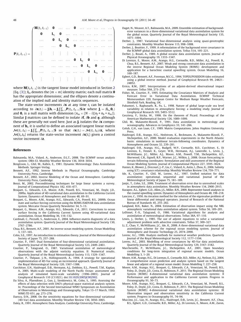
48 A.M. Moore et al. / Progress in Oceanography 91 (2011) 34–49

Pðti; ti�1Þ ¼

Mðti; ti�1Þ 0 . . . . . . 0 . . . . . . . . . . . . . . .

0 Inf0 . . . . . . . . . . . . . . . . . . . . .

. . . 0 Inb0 . . . . . . . . . . . . . . . . . .

. . . . . . 0 Inm 0 . . . . . . . . . . . . . . .

..

. ... ..

. ... . .

. ... ..

. ... ..

. ...

. . . . . . . . . . . . 0 Inf0 . . . . . . . . .

. . . . . . . . . . . . . . . 0 Inb0 . . . . . .

. . . . . . . . . . . . . . . . . . 0 Inm 0 . . .

..

. ... ..

. ... ..

. ... ..

. ... . .

. ...

0BBBBBBBBBBBBBBBBBBBBBB@

1CCCCCCCCCCCCCCCCCCCCCCA

where M(ti, ti�1) is the tangent linear model introduced in Section 2(Eq. (3)); Im denotes the (m �m) identity matrix; each null matrix 0has the appropriate dimensions; and the ellipses denote a continu-ation of the implied null and identity matrix sequences.

The state-vector increments dx at any time ti can be isolatedaccording to dxðtiÞ ¼ Jihi ¼ Ji

Qik¼1Pðtk; tk�1ÞSdz where Ji ¼ ðInm 0cÞ

and 0c is a null matrix with dimension (nm � (N � i)(nf + nb + nm)).Similar J matrices can be defined to isolate df, db and g, althoughthese are generally not used here. Just as Ji isolates the dx compo-nent of hi, it is useful to define an associated tangent linear matrixMðti; t0Þ ¼ Ji

Qik¼1Pðtk; tk�1ÞS so that dxðtiÞ ¼Mðti; t0Þdz, where

M(ti, t0) returns the state-vector increment dx(ti) given a controlvector increment dz.

References

Balmaseda, M.A., Vidard, A., Anderson, D.L.T., 2008. The ECMWF ocean analysissystem: ORA-S3. Monthly Weather Review 136, 3018–3034.

Bengtsson, L., Ghil, M., Kallen, E., 1981. Dynamic Meteorology: Data AssimilationMethods. Springer-Verlag.

Bennett, A.F., 1992. Inverse Methods in Physical Oceanography. CambridgeUniversity Press, Cambridge.

Bennett, A.F., 2002. Inverse Modeling of the Ocean and Atmosphere. CambridgeUniversity Press, Cambridge.

Benzi, M., 2002. Preconditioning techniques for large linear systems a survey.Journal of Computational Physics 182, 418–477.

Broquet, G., Edwards, C.A., Moore, A.M., Powell, B.S., Veneziani, M., Doyle, J.D.,2009a. Application of 4D-variational data assimilation to the California CurrentSystem. Dynamics of Atmospheres and Oceans 48, 69–91.

Broquet, G., Moore, A.M., Arango, H.G., Edwards, C.A., Powell, B.S., 2009b. Oceanstate and surface forcing correction using the ROMS-IS4DVAR data assimilationsystem. Mercator Ocean Quarterly Newsletter 34, 5–13.

Broquet, G., Moore, A.M., Arango, H.G., Edwards, C.A., 2011. Corrections to oceansurface forcing in the California Current System using 4D-variational dataassimilation. Ocean Modelling 36, 116–132.

Cardinali, C., Pezzulli, S., Andersson, E., 2004. Influence-matrix diagnostic of a dataassimilation system. Quarterly Journal of the Royal Meteorological Society 130,2767–2786.

Chua, B.S., Bennett, A.F., 2001. An inverse ocean modeling system. Ocean Modelling3, 137–165.

Cohn, S.E., 1997. An introduction to estimation theory. Journal of the MeteorologicalSociety of Japan 75, 257–288.

Courtier, P., 1997. Dual formulation of four-dimensional variational assimilation.Quarterly Journal of the Royal Meteorological Society 123, 2449–2461.

Courtier, P., Talagrand, O., 1987. Variational assimilation of meteorologicalobservations with the adjoint vorticity equation. II: Numerical results.Quarterly Journal of the Royal Meteorological Society 113, 1329–1347.

Courtier, P., Thépaut, J.-N., Hollingsworth, A., 1994. A strategy for operationalimplementation of 4D-Var using an incremental approach. Quarterly Journal ofthe Royal Meteorological Society 120, 1367–1388.

Curchitser, E.N., Haidvogel, D.B., Hermann, A.J., Dobbins, E.L., Powell, T.M., Kaplan,A., 2005. Multi-scale modeling of the North Pacific Ocean: assessment andanalysis of simulated basin-scale variability (1996–2003). Journal ofGeophysical Research 110 (C11021). doi:10.1029/2005JC002902.

Da Silva, A., Pfaendtner, J., Guo, J., Sienkiewicz, M., Cohn, S., 1995. Assessing theeffects of data selection with DAO’s physical-space statistical analysis system.In: Proceedings of the Second International WMO Symposium on Assimilationof Observations in Meteorology and Oceanography, Tokyo 13–17 March, 1995.WMO.TD 651, pp. 273–278.

Daescu, D.N., 2008. On the sensitivity equations for four-dimensional variational(4D-Var) data assimilation. Monthly Weather Review 136, 3050–3065.

Daley, R., 1991. Atmospheric Data Analysis. Cambridge University Press, Cambridge.

Daget, N., Weaver, A.T., Balmaseda, M.A., 2009. Ensemble estimation of background-error variances in a three-dimensional variational data assimilation system forthe global ocean. Quarterly Journal of the Royal Meteorological Society 135,1071–1094.

Derber, J., 1987. Variational four-dimensional analysis using quasi-geostrophicconstraints. Monthly Weather Review 115, 998–1008.

Derber, J., Bouttier, F., 1999. A reformulation of the background error covariance inthe ECMWF global data assimilation system. Tellus 51A, 195–221.

Derber, J., Rosati, A., 1989. A global oceanic data assimilation system. Journal ofPhysical Oceanography 19, 1333–1347.

Di Lorenzo, E., Moore, A.M., Arango, H.G., Cornuelle, B.D., Miller, A.J., Powell, B.,Chua, B.S., Bennett, A.F., 2007. Weak and strong constraint data assimilation inthe inverse Regional Ocean Modeling System (ROMS): development andapplication for a baroclinic coastal upwelling system. Ocean Modelling 16,160–187.

Egbert, G.D., Bennett, A.F., Foreman, M.C.G., 1994. TOPEX/POSEIDON tides estimatedusing a global inverse method. Journal of Geophysical Research 99, 24821–24852.

Errico, R.M., 2007. Interpretations of an adjoint-derived observational impactmeasure. Tellus 59A, 273–276.

Fisher, M., Courtier, P., 1995. Estimating the Covariance Matrices of Analysis andForecast Error in Variational Data Assimilation. ECMWF TechnicalMemorandum 220, European Centre for Medium Range Weather Forecasts,Shinfield Park, Reading, UK.

Fukumori, I., Raghunath, R., Fu, L., 1998. Nature of global large-scale sea levelvariability in relation to atmospheric forcing: a modeling study. Journal ofGeophysical Research 103, 5493–5512.

Gesztesy, F., Sticka, W., 1998. On the theorem of Picard. Proceedings of theAmerican Mathematical Society 126, 1089–1099.

Ghil, M., Malanotte-Rizzoli, P., 1991. Data assimilation in meteorology andoceanography. Advances in Geophysics 33, 141–266.

Golub, G.H., van Loan, C.F., 1989. Matrix Computations. Johns Hopkins UniversityPress.

Haidvogel, D.B., Arango, H.G., Hedstrom, K., Beckmann, A., Malanotte-Rizzoli, P.,Shchepetkin, A.F., 2000. Model evaluation experiments in the North Atlanticbasin: simulations in nonlinear terrain-following coordinates. Dynamics ofAtmospheres and Oceans 32, 239–281.

Haidvogel, D.B., Arango, H.G., Budgell, W.P., Cornuelle, B.D., Curchitser, E., DiLorenzo, E., Fennel, K., Geyer, W.R., Hermann, A.J., Lanerolle, L., Levin, J.,McWilliams, J.C., Miller, A.J., Moore, A.M., Powell, T.M., Shchepetkin, A.F.,Sherwood, C.R., Signell, R.P., Warner, J.C., Wilkin, J., 2008. Ocean forecasting interrain-following coordinates: formulation and skill assessment of the RegionalOcean Modeling System. Journal of Computational Physics 227, 3595–3624.

Haines, K., Blower, J., Drecourt, J.-P., Liu, C., Vidard, A., Astin, I., Zhou, X., 2006. Salinityusing S(T): covariance relationship. Monthly Weather Review 134, 759–771.

Ide, K., Courtier, P., Ghil, M., Lorenc, A.C., 1997. Unified notation for dataassimilation: operational, sequential and variational. Journal of theMeteorological Society of Japan 75, 181–189.

Janjic, T., Cohn, S.E., 2006. Treatment of observation error due to unresolved scalesin atmospheric data assimilation. Monthly Weather Review 134, 2900–2915.

Kurapov, A.L., Egbert, G.D., Allen, J.S., Miller, R.N., 2009. Representer-based analyses inthe coastal upwelling system. Dynamics of Atmospheres and Oceans 48, 198–218.

Lanczos, C., 1950. An iteration method for the solution of the eigenvalue problem oflinear differential and integral operators. Journal of Research of the NationalBureau of Standards 45, 255–282.

Langland, R.H., Baker, N., 2004. Estimation of observation impact using the NRLatmospheric variational data assimilation adjoint system. Tellus 56, 189–201.

LeDimet, F.-X., Talagrand, O., 1986. Variational algorithms for analysis andassimilation of meteorological observations. Tellus 38A, 97–110.

Lewis, J., Derber, J., 1985. The use of adjoint equations to solve a variationaladjustment problem with advective constraints. Tellus 37, 309–327.

Li, Z., Chao, Y., McWilliams, J.C., Ide, K., 2008. A three-dimensional variational dataassimilation scheme for the regional ocean modeling system. Journal ofAtmospheric and Oceanic Technology 25, 2074–2090.

Lorenc, A.C., 1986. Analysis methods for numerical weather prediction. QuarterlyJournal of the Royal Meteorological Society 112, 1177–1194.

Lorenc, A.C., 2003. Modelling of error covariances by 4D-Var data assimilation.Quarterly Journal of the Royal Meteorological Society 129, 3167–3182.

Marchesiello, P., McWilliams, J.C., Shchepetkin, A.F., 2001. Open boundaryconditions for long-term integration of regional oceanic models. OceanModelling 3, 1–20.

Moore, A.M., Arango, H.G., Di Lorenzo, E., Cornuelle, B.D., Miller, A.J., Neilson, D.J., 2004.A comprehensive ocean prediction and analysis system based on the tangentlinear and adjoint of a regional ocean model. Ocean Modelling 7, 227–258.

Moore, A.M., Arango, H.G., Broquet, G., Edwards, C.A., Veneziani, M., Powell, B.S.,Foley, D., Doyle, J.D., Costa, D., Robinson, P., 2011. The Regional Ocean ModelingSystem (ROMS) 4-dimensional variational data assimilation systems: IIPerformance and application to the California Current system. Progress inOceanography 91, 50–73.

Moore, A.M., Arango, H.G., Broquet, G., Edwards, C.A., Veneziani, M., Powell, B.S.,Foley, D., Doyle, J.D., Costa, D., Robinson, P., 2011. The Regional Ocean ModelingSystem (ROMS) 4-dimensional variational data assimilation systems: IIIObservation impact and observation sensitivity in the California Currentsystem. Progress in Oceanography 91, 74–94.

Muccino, J.C., Luo, H., Arango, H.G., Haidvogel, D.B., Levin, J.C., Bennett, A.F., Chua,B.S., Egbert, G.D., Cornuelle, B.D., Miller, A.J., Di Lorenzo, E., Moore, A.M., Zaron,

A.M. Moore et al. / Progress in Oceanography 91 (2011) 34–49 49

E.D., . The inverse ocean modeling system. Part II: Applications. Journal ofAtmospheric and Oceanic Technology 25, 1623–1637.

Paige, C.C., Saunders, M.A., 1975. Solution of sparse indefinite systems of linearequations. SIAM Journal on Numerical Analysis 12, 617–629.

Powell, B.S., Arango, H.G., Moore, A.M., Di Lorenzo, E., Milliff, R.F., Foley, D., 2008.4DVAR data assimilation in the intra-Americas Sea with the Regional OceanModeling System (ROMS). Ocean Modelling 25, 173–188.

Powell, B.S., Moore, A.M., 2009. Estimating the 4DVAR analysis error from GODAEproducts. Ocean Dynamics 59, 121–138.

Ricci, S., Weaver, A.T., Vialard, J., Rogel, P., 2005. Incorporating state-dependenttemperature-salinity constraints in the background-error covariance ofvariational ocean data assimilation. Monthly Weather Review 133, 317–338.

Sasaki, Y., 1970. Some basic formulations in numerical variational analysis. MonthlyWeather Review 98, 875–883.

Shchepetkin, A.F., McWilliams, J.C., 2003. A method for computing horizontalpressure-gradient force in an oceanic model with a nonaligned vertical grid.Journal of Geophysical Research 108 (C3). doi:10.1029/2001/JC001047.

Shchepetkin, A.F., McWilliams, J.C., 2005. The regional oceanic modeling system(ROMS): a split explicit, free-surface, topography-following-coordinate oceanicmodel. Ocean Modelling 9, 347–404.

Stammer, D., Wunsch, C., Giering, R., Eckert, C., Heimbach, P., Marotzke, J., Adcroft,A., Hill, C.N., Marshall, J., 2002. The global ocean circulation during 1992–1997estimated from ocean observations and a general circulation model. Journal ofGeophysical Research 107. doi:10.1029/2001JC000888.

Talagrand, O., Courtier, P., 1987. Variational assimilation of meteorologicalobservations with the adjoint vorticity equation. I: Theory. Quarterly Journalof the Royal Meteorological Society 113, 1321–1328.

Talagrand, O., 1997. Assimilation of observations, an introduction. Journal of theMeteorological Society of Japan 75, 191–209.

Thacker, W.C., 1989. The role of the hessian matrix in fitting models tomeasurements. Journal of Geophysical Research 94, 6177–6196.

Thacker, W.C., Long, R.B., 1988. Fitting dynamics to data. Journal of GeophysicalResearch 93, 1227–1240.

Tarantola, A., 1987. Inverse Problem Theory: Methods for Data Filtering and ModelParameter Estimation. Elsevier, Amsterdam.

Trémolet, Y., 2006. Accounting for an imperfect model in 4D-Var. Quarterly Journalof the Royal Meteorological Society 132, 2483–2504.

Trémolet, Y., 2007. Model-error estimation in 4D-Var. Quarterly Journal of the RoyalMeteorological Society 133, 2671280.

Tshimanga, J., 2007. On a Class of Limited Memory Preconditioners for Large-scaleNonlinear Least-squares Problems. PhD Thesis, Facultés Universitaires Notre-Dame de la Paix, Namur, Belgium.

Tshimanga, J., Gratton, S., Weaver, A.T., Sartenaer, A., 2008. Limited-memorypreconditioners with application to incremental variational data assimilation.Quarterly Journal of the Royal Meteorological Society 134, 751–769.

Weaver, A.T., Courtier, P., 2001. Correlation modelling on the sphere using ageneralized diffusion equation. Quarterly Journal of the Royal MeteorologicalSociety 127, 1815–1846.

Weaver, A.T., Deltel, C., Machu, E., Ricci, S., Daget, N., 2005. A multivariate balanceoperator for variational ocean data assimilation. Quarterly Journal of the RoyalMeteorological Society 131, 3605–3625.

Weaver, A.T., Vialard, J., Anderson, D.L.T., 2003. Three- and four-dimensionalvariational assimilation with a general circulation model of the tropical PacificOcean. Part I: Formulation, internal diagnostics and consistency checks.Monthly Weather Review 131, 1360–1378.

Wunsch, C., 1996. The Ocean Circulation Inverse Problem. Cambridge UniversityPress, Cambridge.

Wunsch, C., 2006. Discrete Inverse and State Estimation Problems: WithGeophysical Fluid Applications. Cambridge University Press, Cambridge.

Zhu, Y., Gelaro, R., 2008. Observation sensitivity calculations using the adjoint of thegridpoint statistical interpolation (GSI) analysis system. Monthly WeatherReview 136, 335–351.