Progress in Nonlinear Differential Equations and Their Applications Volume 9

Editor

Haim Brezis Universite Pierre et Marie Curie Paris and Rutgers University New Brunswick, N.J.

Editorial Board

A. Bahri, Rutgers University, New Brunswick John Ball, Heriot-Watt University, Edinburgh Luis Cafarelli, Institute for Advanced Study, Princeton Michael Crandall, University of California, Santa Barbara Mariano Giaquinta, University of Florence David Kinderlehrer, Carnegie-Mellon University, Pittsburgh Robert Kohn, New York University P. L. Lions, University of Paris IX Louis Nirenberg, Ncw York University Lambertus Peletier, University of Leiden Paul Rabinowitz, University of Wisconsin, Madison

Manuel D. P. Monteiro Marques

Differential Inclusions in Nonsmooth Mechanical Problems

Shocks and Dry Friction

1993 Springer Basel AG

Manuel D. P. Monteiro Marques Centro de Matematica e Aplica<;6es Fundamentais Av. Prof. Gama Pinto, 2 1699 Lisboa Codex Portugal

A CIP catalogue record for this book is available from the Library of Congress, Washington D.C., USA

Deutsche Bibliothek Cataloging-in-Publication Data Monteiro Marques, Manuel D. P.: DifferentiaJ inclusions in nonsmooth mechanical problems : shocks and dry friction / Manllel D. P. Monteiro Marques. -Basel ; Boston ; Berlin : Birkhăuser, 1993

(Progress in nonlinear differential eqllations and their applications ; Val. 9)

NE:GT

ISBN 978-3-0348-7616-2 ISBN 978-3-0348-7614-8 (eBook)

DOI 10.1007/978-3-0348-7614-8

This work is subject ta copyright. Al! rights are reserved, whether the whole ar part of the material is concerned, specifical!y the rights of translation, reprinting, re-use of il!llstrations, broadcasting, reproduction on microfilms ar in other ways, and storage in data banks. For any kind of use permission of the copyright owner must be obtained.

© 1993 Springer Base! AG Originally pub!ished by Birkhăuser Verlag Base! in 1993 Camera-ready copy prepared by the authar Printed on acid-free paper produced from ch1arine-free pulp

9 8 7 6 5 432 1

Contents

lntroduction

Chapter 0

Preliminaries

0.1 Functions of bounclecl varia.tion

0.2 Compactness results for functions of boundecl variation

0.3 Convergence in the sense of fillecl-in graphs

0.4 Geometrical inequalities

Chapter 1

Regularization and Graph Approximation of a Discontinuous Evolution

VII

1

10

15

20

1.1 Introcluction 27

1.2 Preliminary estimates 30

1.3 Limit functions 35

1.4 The solution 39

1.5 Graph convergence 42

Chaptcr 2

Swccping Processes by Convcx Sets with Noucrnpty Intcrior

2.1 Introcluction 45

2.2 Continuous convex set in iirbitrary clinwnsion: prdimin<t.ry results 46

2.3 Continuous conn·x sct in arbitntry dinwnsion: algorithm ancl existence 50

2.4 Lower scmicoutimwus convex sct in fi1titc dimeusion 59

Chapter 3

Inclastic Shocks wit.h or without Fridion: Exist.cncc Rcsults

3.1 Introcluction

3.2 Frictionless inelastic slwcks

3.3 Inelastic slwcks with friction

Chaptcr 4

Extcrnally Induccd Dissip<tt.ivc Collisions

4.1 Formulation of tJw prohlcm

4.2 Existence of a solutiou

4.3 Complements

72

82

95

112

117

126

Chapter 5

Further Applications and Related Topics

5.1 A dass of second-order differential inclnsions

5.2 Lipschitz approximations of sweeping processes

5.3 An application of differential inclusions to quasi-statics

5.4 Additional references

Bibliography

Index

Index of Notation

132

141

155

162

167

177

179

Introduction

This book is devoted to the sndy of some clifferentia.l inclusions

motivated by Mechanics and of existcnce rcsults for the dynamics of systems

with inelastic shocks, with or without friction. This ensures a certain unity of

subject, techniques and applications, at the price of not including some earlier

works [Mon 1-4] .

In the introductory Chapter 0, sevcral essentia.l mathematical tools

(either recent or recently rediscoven~d) are presented. l\1ainly they concern

functions of bouncled variation defincd in real interva.ls ( deriva.tion of Stieltjcs

measures, compactness results. convergencrc in tlw sense of graphs) a.ncl

geometrical inequa.lities.

In Chapters 1 and 2, Ivforea.u' s swecpiug process is considcred; this is a

first-order differential inclusion

(1)

where the right-ha.nd siele is tla:' outw<~nl uormal cone to a convex sct C( t) a.t a

point u( t) of a rea.l Hilhert SJMCe H. This a.h.-;tr<•.ct formulation encompasses

several practical sitnations iu lVIeclwuics, sucl! as water falling in a. cavity

[Mor 1], the dynamics of syst.ems with perfect unilatera.l constraints

[Mor 15, 16], pla.sticity and the evolntiou of dastoplastic systems [Mor 3, 17].

In Chapter 1, hased on [1vion 5], it is assumed tha.t the rnoving convex

set, 1. e., the multifunction t-> C( t) has rigl!t-contiuuous hounded variation

(iri short, it is said tobe rcbv). Thcn i\ uuique rcbv solution of (1) is known to

exist, for any prescribed admissihle iuit.ia.l valne. It is provccl here that even in

this case the regulariza.tion tecl!uiqn<' of Yosida ( or l\Iorean- Y osida) still gi ves

a sequence of absolutely continuous functions that couverge to the solution.

Since the latter ma.y be discontinnous, iu geueral thc convergence is not

uniform but "in the sense of filled-in graphs". This numerically meaningful

notion of convergence, previously introduced in Chapter 0, looks bouncl to gain

importance, as more and more discontinuous problems are currently being

treatecl. Several other technical results ou conV<'l")!,ence i\Te given.

Chapter 2, which is basecl on (Mon 6, 7], eieals with the case of a convex

set C( t) which is not necessarily of boundecl variation in time but has

nonempty interior insteacl. The existence of a cbv ( continuous with boundecl

variation), respectively of an rcbv solution, is proved for two cases: a) the

multifunction t -+ C( t) is continuous in the sense of Hausdorff distance and the

Hilbert space has a.rbitrary dimension; b) the convex set 1s lower

semicontinuous from the right ancl H is finite dimensional. Although the

starting point is the well-known discrctization technique of Moreau ( the

catching-up algorithm) the proofs are substantially different and recent

technical aclvances are needecl. Cliapter 2 also contains a raueiom or

parametrized version of inclusion (1), as weil as some a priori bounds and a

study of the dependence on tl1e clata.

Chapter 3, partially basecl on (!\Ion S], is concerned with the problem of

the dynamics of a mechanical systcm vvith a finite number of clegrees of

freeclom, subject to a unique unilateral constraint and experiencing inelastic

shocks. The constraint is expressed by an inequality f( q) ::::; 0, defining a region

L. In the frictionless case, the synthetic modern formulation of Moreau

(Mor 11 J gives rise to the second-order differential inclusion:

(2) p(t, q(t)) dt- duE NV(q(t))(u(t)),

where u=q 1s the rcbv velocity, p is a force fiele! ancl V(q(t)) is the (convex)

tangent cone to L at the position q( t). The existence of a solution to (2) is

proved by constructing a suitable sequence ( qn) of approximants of the motion

and extracting a uniformly convergcnt subsequence. The rather long proof uses

some of the techniques of Cl1aptPr 2, thus explaining a somewhat weak

regularity assumption on L (its houuda.ty only neecls to be e1 ).

With a similar approach, it is shown that there exists at least one

solution to the problem with Coulomb' s isotropic friction, expressed by a

differential inclusion that can lw writtt'll as:

(3) - u(t)E projT(q(l)) NC(q(t))(d11.-p(t, q(t)) dt),

where C(q(t)) is the friction cone and T(q(t)) is the tangenthyperplane to L at

q( t). In this currently active research field there remain many open problems,

e. g., to find conclitions ensming uniqueness of the solution and to prove

existence in the presence of more than one unilateral constraint.

In Chapter 4, it is stuclied a problem clerivecl from (2) and involving

what may be called externally induced collisions ( or shocks or contacts ). An

"activation multifunction" t-> A( t) 1s given, with values in a finite set

{1, ... , z;} and which selects among the constraints J1 ( q) :<::; 0, ... , fv( q) :<::; 0

those that are active at time t. The corresponding differential inclusion is the

following:

(4) p(t,q(t))dt-d·nc NW(A,I,q(t))(u.(t)),

where W(A, t, q(t)) is a convex set, lower semicontinuous with respect to t,

associated to A. By exploit.ing the introcluccd techniques and fixed point

theorems, the existencc of solution is obta.ined, although not the uniqueness.

The relation between the problems of iuelastic shocks ancl of inducecl collisions

is also cliscussed.

In the final Chaptcr 5, some directions of rcsearch tha.t can be linked to

the present exposition are reviewed. A short presentation is ma.clc of three

works: 1) existence for some second-orcler differential inclusions by C. Castaing;

2) the approximation techniques for differential inclusions recently devcloped

by M. Valadier ancl A. Gavioli; ancl 3) a.pplication of lower semicontinuous

differential inclusions to qua.si-statics by Chraibi. In sect.ion 5.4 the list of

references on related subjects is expancled.

It is assumed that the reader is fa.miliar with hasic concepts of Real

Analysis, General Topology ancl some Functicmal Anillysis. In particular, a

preliminary knowledge of cvolntion equotions a.ncl of set-va.lued analysis is

aclvisable. Nevertheless, sonw effort was clone in orclPr to render the reading as

self-contained as possible (in wha.t gocs hcyoncl stanclard text books).

I am deeply gra.teful to Prof. .Jeau .Jacques Moreau (Montpellier), who

introduced me to the fielcl ancl snggest.ed most of t!te rcsearc!t problems, for his

warm-hearted support ancl enlight<~uecl scieutific gnicl<mce.

I am also gratefnl to Profs. Clt<ules Castaing ancl l'v1ichel Valadier

(Montpellier) for stimulating disr:ussious on the suhject; to Prof. Pana.giotis

Panagiotopoulos (Thessaloniki ancl Aaclwn) for encouraging me to write the

book; to E. F. Beschler (Birkhiinser) ancl to my colleagues Owen Brison, .Joäo

Martins (IST), Augusto Franeo de Olivcira, Lnis Saraiva ancl Luis Trabucho

for helping improve my Euglish; to Bntto Lumo and Armanclo Macha.do for

their help with hardware aucl software; ancl to colleagues ancl friencls at the

Mathematical Department of the Science Faculty FCUL (Faculdacle de

Ciencias da Universidade cle Lisboa) ancl at the Research Center CMAF

(Centro de Matematica e Aplica~öes Funclamentais) for creating such a warm

and joyful work environment, even uncler sometimes adverse circumstances.

I am indebted to several institutions that supported this research at

different stages throughout the years, namely to FCUL, to the French

Government, to Funcla<;a.o Calouste Gulbenkian (Lisboa) ancl to the former

INIC (Instituto Nacional de Investiga<;äo Cientifica).

I have great pleasure m thanking the publishers for fruitful

collaboration, in particular by Dr. Thomas Hintermann.

Lisboa, March 1993 JVIanuel D. P. Monteiro Marques

Chapter 0

Preliminaries

0.1. Fundions of bounded variation In this section, we gather some information on functions of bounded variation

of a single real variable. For a detailed study, we refer to [Mor 10] which we

use extensively.

Let I be a nonempty real interval and H be a real Hilbert space, with

norm II II ( although for part of the results we coulcl take, more generally, a

real Banach space or a metric space). We consider functions u: I-;H. For

every t different from the possible right end of the interval, ·u+( t) denotes the

righ t-limi t

<t+(t) =lim 5_ 1, 5 > 1 ·u.(s),

if it exists. The left-limit 11.-(t) is clefinecl similarly. If t is the right endpoint of

I, we agree to write v+(t)=<t(t). If t is the left enclpoint, we write u-(t)=u(t);

if u(t) is an initial datum, say an initial velocity, this convention means that

u( t) convcys some abridgecl informa.tion on the system history before t.

If they are clefinecl everywhere in an open interval, then u+ is a right­

continuous function ancl u- is a lcft-continuous function, i.e., ( u+)+ = u+ and

(u-)-o.cu-. Also, (u-)+=·u+ and (u+)-=u-.

The variation of ·u. in a subinterval J of I is the nonnegative extencled

real number

(1) 11

va.r(u., J)= sup .L llu(t;) -u(ti-1) II , i=l

where the supremum is taken in [0, +=] with respcct to all the finite sequences

io < t1 < ... < tn of points of J ( n is arbi trary). For any singleton,

var( u, { t}) = sup 0 = 0. More generally, var("u., J) = 0 if and only if u is constant

on J. We also wri te var( u; a., b) insteatl of va.r( u.; [ a., b]) , wi th the property that

var(u; a, c)=var(u; a., b) + var(<Lj b, c).

The function u: I_., H is saicl of bmmded variation on I if and only if

var( u, I) < +oo. We often say that ·u. is bv or is a bv function and write

u E b1J(I, H) . The set of functions of bouncled variation is a linear space, since

2 Chnpter 0: Preli1ninarics

var(>.u+ßv; I) S:: I AI var(u, I)+ I jJ I var('u, I). If 11 is bv, the above aclclition

rule implies that there exists a. nondecreasing function Vu: I---> IR ( called a

variation function of u) such that

(2) li[a., b] C I: var(n; a., b) = V11(b)- Vu(a);

for instance, Vu( a) = var(·u; c, a) (resp. - var( u; a., c)) if a ~ c (resp. if a < c)

where CE I is fixecl. Conversely, (2) implies that u is of locally bounded

variation (lbv for short), that is, u has finite va.riation on any compact

subinterval of I. If 1l is Lipschitz-continuous (resp. absolutely continuous) then

Vu is Lipschi tz-continuous ( resp. absolutcly continuous) ancl conversely. In

fact, assuming for example that Vu is Lipsdlitz-continnous with constant k,

then

II u(b)-u(a.) II S:: var('u; a, b)= V11(b)- Vu(a) S:: k I b-al.

A bv function u clcfinecl on [0, T] possesses left-limits in ]0, T] and right­

limits in [0, T[. A variation fnnct.ion V 11 is ldt, or right or simply continuous

at t if and only if the same holcls with the function lt. This is a consequence of

formttlas such as ( see [lVIor 10] Prop.4.3):

limsTi /11t(s)--u.(t) II = lim,llva.r(u; s, t)= Vu(t)- vu-(t).

As it is well known that a nonclecreasing real function, such as Vu, has

a countableset of cliscontinuit.y point.s, tlw Sillllf' is true for any bv function 1t.

It can be shown that, if u is hv, tlwn ·u.- ancl n+ are hoth bv functions,

wi th for instance

We now clcfine the integra.l witl1 rcspect to the differential measure of u

of a continuous real function rp on I wlwse 'illJlport, rcla.tive to I, is compact;

we may write <jJE'JG(I). vVe clmote by '1' the sct of finite subsets of I. If P

belongs to '1', its elements, which we call nodes, ma.y be ordered, say P:

fv < t1 < ... < t". The elements of '1' are themselves orclered by inclusion:

P ~ Q iff P :J Q. Hence, '1' bccomes a directecl set ancl we can ta.ke Iimits of

families indexed on '1', that is of nets or generalizecl sequences. Let us say that

8 is an intercala.tor if it associates with evny P f '1' and every i an element

8 P,iE [ ti-l, tJ If 1l is a bv function ancl (} is an intercalator, we may define the

(Riemann-Stieltjes) sums, indexed by PE '1',

(3)

0.1 Functions of bonnded variation 3

and prove that they converge to a limit, which IS independent of the

intercalator; moreover, the convergence is uniform with respect to 8. We

define:

(4) j rfidu. =limP<':P S(rjJ,P,8; u).

If [ a, b] is a compact subinterval of I containing the support of r/J, then it

follows from the above definition that:

(5) II j rP du II :S ma.x I rP I var(u; a, b).

This shows that the linear map r/J-> J r/J du from %(I) to His continuous and so

is a vector measme on I, in the sense of Bombaki. This H-valuecl measure is

called the differential measure or Stieltjes measure of the function u E bv( I, H) and denoted by d·u. To approxima.te the va.lue of the integral (4) we may use

the following: let E > 0 and let an intcrval [ a, b] contain the support of r/J; by

uniform continuity of ifJ on [ a, b], we choose P with nodes so close that

I rfi(t)-rfi(s) I :S E, for every i ancl every s, t in [ti-l• ti] ; then, P' ::::> P with P'=(t'i) implies that ([Mor 10], (6.10)):

(6) II j ,Pdu- i~l r/!(BP')(u(t';)-·u.(t'i-l)) II :SE var(u.; a,b).

The map u-> du is linear, wi th v a.l ues in the real linear space of all H­

valued measures. If the vector functiou 11. is a constant, then du= 0. The

converse is true if u is right-continuous (a.lternatively, left-continuous) in the

interior of I.

If u is a step function, there is PE 'P such that ·u is constant on every

interval of P. In this case, the integral ( 4) is given by

(7)

Only the nodes containecl in the support of rP need to be considered in (7). In

other words, the differential mea.sure d·u equa.ls the sum of a finite collection of point (Dirac) measures, placecl at the cliscontinuity points of u, their values

being the respective jumps of ·u.:

(8)

This is also true for loca.l step functions: in tha.t case we get in (8) a locally

finite collection of point nwasmes. Tlw fonnula also shows that we may

change the value of 11. at an intcrior point, sa.y tk, without changing the

differential mea.sure.

4 Chapt.er 0: Preliminaries

We next recall some concepts ancl properties of general vector

measures.

A vector measure m on I is majorable iff there exists a nonnegative real

measure p on I such that, for every <PE%(!):

(9) II j <P dm II :::: j I <P I dp .

By the usual decomposition of a function as a clifference of nonnegative

functions, it suffices to verify (9) for nonnegative functions </;t:%+(1). If H has

finite dimension, then any H-valued measnre is majorable.

Consider a majorable H-valued measure, where H is a (real) Hilbert

space. For fixed x EH, the linear map t/>-+ x. J tj> dm from %(I) to !Ii! is a real

measure, denoted by x. m. If II x II :::; 1, we have:

(10) w [ %+(!) : X. J rP dm. :::; II XII J rP dlt :::; J rP dp )

so that x. m. :::; J.l in the sense of the ordering of real measures. The supremum

of the measures x. m with II x II :::; 1 is then a nonnegative real measure :::; p;

it is called the m.odulus or absolute value of m and it is clenoted by I m I or

I dm I . In case H = !Ii!, this is the usual absolute value of a real signecl measure.

By definition, X. J <P dm:::; J t/> I dm I; taking X= II J rP dm II-I J rP dm' we have

(11) II j <P dm II :::; j <P I dm I , W [%+(I).

Consequently, (9) ancl (10) hold with djt replacecl by I dm 1-

A real function h: I-+ !Ii! is sca.la:rly ·integra.ble with respect to m if it is

integrable wi th respect to all real measures x. m, wi th x EH. The integral of h

is then clefined as the element J h dm of H for which

(12) j hd(x.m)=x. j hdm, VuH,

if it exists. This is always the case if m is majorable ancl ht: 1 1( I, I m I ; !Ii!) ancl

then:

(13) II j h dm II :::; j I h I I dm I .

An extension of the dom:inatcd con:uer·gence theorem asserts the

following: let (hn) C 1 1(!, Im I; !Ii!) converge Im. I- almost everywhere to h ancl

let lhn(t)l:::; g(t) for Jml-almost evcry t in I, with gt:l1(I,Im.J;Ifi!+); then

the Iimit h is also an integrable fnnctioa with respect to I m I and

(14) lii,v j h11 rlm= j hdm,

in the sense of the nonn of H.

0.1 Funct ions of boundecl variat.ion 5

An important example of a majorahle H-valuecl meas.ure is the product

of a real measure JL ancl a locally integrable vcctor function m~ c; Lfoc (I, JL; H).

vVe denote i t by m = m~, ;t or dm = m.~, d;t ancl we define:

(15) j <f;dm= j </; m.~,dJl, Y<f;c:'JG(J).

In these circumstances, we say that m admits m.;, as a density relative to fl. Of

course, we may replace m~, by auy ;t-equivalent H-valuecl function: a density

of m may be consiclered as a uniquely clefinecl element of Lfoc (I, f1; H). If JL is

nonnegative, the moclulus measure is given hy I m;, JLI = II m.~ II Jl.

Since any Hilbert space l1as the so-called Raclon-Nikoclym property, it is

true that every majorablc measnre m. is of the ahove form (15) with p equal to

the modulus measure of m.; in ot.her worcls, m ha.s a density with respect to

I ml. For instance, let m=ah 1 , wit.h aEH\{0}, so that J hdm.=h(t)a; then

Jl = I ml = II a II 0 t aud m~, = II all -l a ·

In the special case of a Sticltjes measure d1t of a bv function u it is

known that du is majora.ble and that, in the sense of the ordering of real

rneasures:

(16) I du. I s dVlt.

In fact, for </;c'JG+(I),we haveii5(</;,P,IJ;u.)ll S L,<f;(IJp,;)llu(t;)-1t(t;_])ll

< L,<jJ(IJp,;)(V11(t;)-V11(t;_ 1))=5(</!,P,IJ;V"). This implies that, in the

Iimit with rcspect toP, II .f qJ du II S f ([J dVu , wl1ence f 0 I d·nl S f <P dVu ,

by definition of I d:u I . Notice th<tt, iu geueral, the equality does not hold in

(16): take u collSta.nt except at au interior point of I and obtain

I du I = 0 I d vlt . However' if u. l!as aligned jnmps, i .e.' if for every t c I the

value u( t) belongs to the line segmeut with mdpoints u-(t) ancl n+(t), then

(1 7) I dnl = dV1,.

Conversely, ( 17) implies that ·u. has aligrwcl j umps, because H has a strictly

convex norm. It is clear t.ha.t ( 17) applies to right-continuous bv functions. The

rneasure I du I is also callccl tlw mws11.re of total va.riation of u ( compare (17)

and (2) to obtain J I dnl =var(n) ).

Like real measures, vector measurcs are uniquely deterrnined by the

values they take on compact subinterYals, that is by the integrals of the

respective characteristic functious. These are usually denotecl hy the letter X:

XA ( x) = 1, if x c; A ancl 0 otherwise. For Stidtjes measures, we have:

6 Cl!itpt.er 0: Prelirninaries

(18) J d·tL = j \[ b] du. = ·u.+( b)- ·u.-( a.) , [ a, b] a,

with the particular case of a singleton:

(19) J du= u+( a)- u-( a) . {a}

This follows by approaching the cha.ra.cteristic function by a sequence of

continuous functions and applying the dominated convergence theorem. Since

X[a, bJ =X{ a} +X Ja, bJ , (18) and ( 19) imply that

(20) j Ja, bJ d1L = 1L+( b)- 1L+( a) .

By similar reasonings,

(21) J du=·u-(b)-·tqa.), [a, h[

(22) j d11. = ·u-(b)- ·u.+(a.) . Ja, I•[

A consequence of this and of (1L+)+=u+ a.nd (·u.-)-=u- is that

du+= du (if u is right-continuous at the left end of I) and du-= du (if u is left-

continuous at the right end of I).

Let J be a nonempty subinterval of I. \Ve denote by uJ the restriction

of u to J; d( u J) is the differential measure of u J . Let '(!; be the extension of

.p E. %( J) to I with zero va.lue outside J (notice that '(!; belongs to

1 1(!, I du I; IR)). The meas·nn ·indu.ced by du. on J is denoted by ( du.)J and has

the defini tion:

(23) j .P (du) J = j '(!; du , V .P E. %( J) .

It can be shown that (du)J equals the sum of d(uJ) and the following measures

on J: (a) the measure {-LL(a)-u-(a))•.\1 , if J contains its left end a; (b) the

measure (u+(b)-u(b))o 6 if J contains its right end b. The conventions about

endpoints of I apply here. In the pa.rticular case of a singleton J={a} (a=b)

we have ( du)J = ( 11.+( a)- 1L-( a.)) <\., wherea.s d( 11.J) = 0. While ( du)J -:j:. d( uJ) may look inconvenient, everything runs smoothly with the variation:

var(u, J)=var(uJ, J).

The Bourbaki construction of a Z-va.lued measure through a bilinear

map <P: X x Y---> Z involving three Ba.na.ch spa.ces ca.n be specialized to the case

where <P: HxH-.IR is the scalar product <P(x,y)=x.y. If m is a majorable

H-valued measure, we sta.rt by defining the integral J f. dm as a linear

continuous function of f E. 1 1(!, I m I ; H) with values in IR. Since the linear

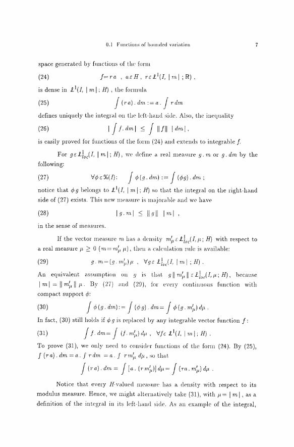
0.1 Fuuctious of houuded variat.iou 7

space generated by functions of tlw form

(24) f= ra , a.~ H, rc1. 1(l, I ml ; IR) ,

is densein 1 1(I, I ml; H) , the fonnula

(25) j (·ra). drn := a.. j rdm

defines uniquely the integra.l on tlw left-hand side. Also, the inequality

(26) I j f. dml ~ j IIJII I dml,

is easily provecl for functions of the form ( 24) and extencls to integrable f.

For gcl}0 c(I, I ml; H), we define a real mea.sure g. m or g. dm by the

following:

(27) \ltjJE.'.JG(I): j ~(.q.dm) := j (</Jg).dm.;

notice that ~ g belongs to 1 1(1, Im I; H) so that the integral on the right-hancl

siele of (27) exists. This new mea.sure is majora.hle a.ncl we have

(28) I g. ml ~ II r1 II I m I , in the sense of mea.sures.

If the vector measure m has a. clensity m~1 t:l}0 c(I, tt; H) with respect to

a real measure p ~ 0 ( m. = rn.;1 Jt), theu a. calcnlation rnle is a.va.ila.ble:

(29) g.m=(g.m.;1)p, Vgt:l)0 c(I, lml ;H).

An equiva.lent a.ssumption on !J IS that g II m.;, II t:l!oc(I, p; H), because

I m.l = II m~ II p. By (27) ancl (29), for every contiuuous function with

compact support </J:

(30) j </J(g.dm):= j (<f!g).dm= j </J(g.m.~,)dp. In fact, (30) still holcls if 4> g is repla.cecl by a.ny integra.ble vector function f:

(31) j f. dm.= j (f. rn;,) d11, Vfc: L1(I, I ml; H) .

To prove (31), we only neecl to consider functions of the form (24). By (25),

I (ra). dm = a. I rdrn = a. I rm;, dft, so tha.t

j (1·a.).dm.= j[a. (nn.;,)Jdft= j (Ta .. m.;,)dJt.

Notice that every H-va.lued mea.sure ha.s a density with respect to its

modulus measure. Hence, we might a.lterna.tively ta.ke (31 ), with JL = I m I , as a

definition of the integral in its left-ha.nd siele. As an example of the integral,

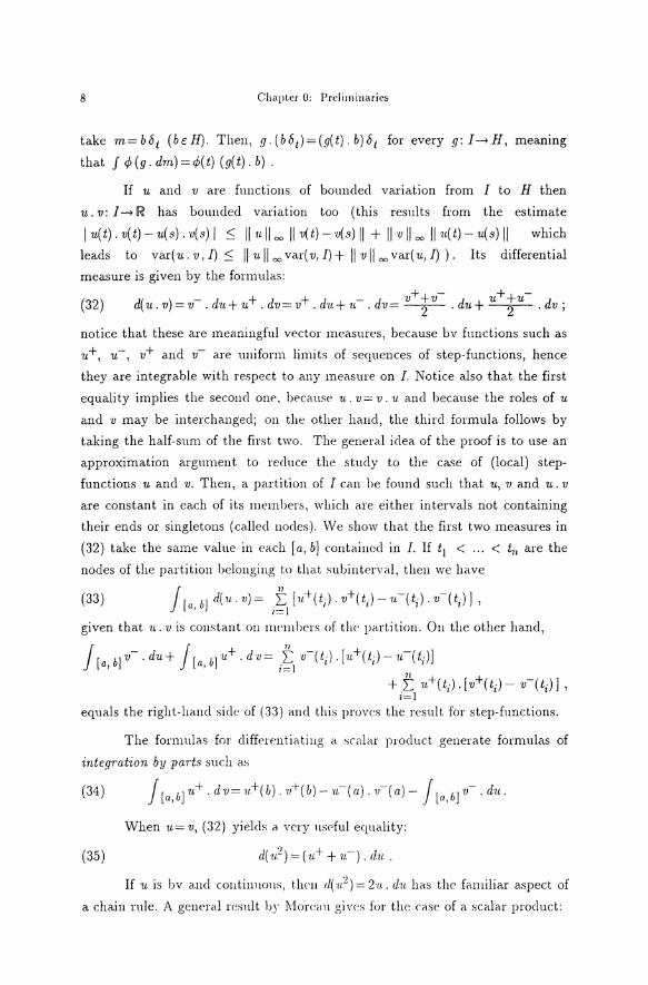
8 Chapt.er 0: Preliminaries

take m=b81 (bcH). Then, g.(b8 1)=(g(t).b)81 for every g:I--"H, meaning

that J</J(g.dm)=<P(t) (g(t).b).

If u and v are functions of bouncled variation from I to H then

u. v: I__" IR ha.s bounded variation too (this results from the estimate

1 u(t). v(t)- u(s). v(s) I s; II ·nll = II v(t)- ·u(s) II + II v II = i11t(t)- u(s) II which

leads to va.r( u. v, I) s; II u II = var( v, I)+ II v II = var( u, I) ) . Its differential

measure is given by the formulas:

d( ) - - d + d - + d· - d - v+ +v- d u+ +u- d · (32) u.v-v. u+u. v-v .. n+1t. v---2-. u+--2-. v,

notice that these are mea.ningful vector measures, because bv fnnctions such as

u+, u-, v+ a.nd v- are uniform limits of sequences of step-functions, hence

they are integra.ble with respect to any measure on I. Notice also that the first

equality implies the seconcl onP, bPcause n. v= ·u. ·u. ancl because the roles of u

and v may be interchanged; on the other hand, the third formula follows by

taking the ha.lf-sum of the first two. The genera.l idea of the proof is to use an

approximation argument to recluce the study to the case of (local) step­

functions u and v. Then, a partition of I c<m be found such that u, v and u. v

are constant in each of its members, wl1ich are either intervals not containing

their ends or singletons ( ca.lled nocles ). W e show tha.t the first two measures in

(32) take the same value in each [ a, b] containecl in I. lf t1 < ... < t,, are the

nodes of the partition belanging to that subinterval, then we have

(33) j 11 + + - -[ b) d( 1/ . . V) = L [ Ii ( t i) , V ( t;) - V. ( t;) . V ( t;) ] 1 a, i=l

given that 1t. v is consta.nt on members of tlw partition. On the other hand,

j [a, b] v-. du+ j [a, b] ·u+. dv= i~l v-(tJ. [·u+(ti)- u-(t;)]

n + + -+ L 1/. ( t;) . [V (t;) - V ( t;) l ) i=l

equals the right-ha.nd siele of (33) and this proves the result for step-functions.

The formulas for differentiatiug a sc;1lar procluct generate formulas of

integration by parts such as

(34) j[a,b(n+.d·u=u+(b).·n+(b)-u.-(a).n-(a.)- Jra,b]v-.du.

(35)

When u= v, (32) yields a very nsdul equality:

d( u2 ) = ( v+ + 11.-) . du .

lf u is bv and continnons, th<·n d("u2 ) = 2n. du has the familiar aspect of

a chain rule. A gent>ral resnlt by JVIor<'<lll gives for the cast> of a. scala.r product:

0.1 Funrtious of bouuded va.riation 9

(36)

To prove this, in view of (35) and of the approximation technique it suffices to

show that u+ . du 2: u- . d1t , for every step-function u; with nodes chosen as

above, we have in fact:

j [a, b] ( u+- u-). du = i~l [·u+( t;)- 1/.-(tJ]. [ u+(ti)- 11.-(ti)] 2: 0 .

Let us end this section with the Moreau-Valaclier extension to Banach­

valued measures of Jeffery' s result on the clerivation of real measures [Jef].

Theorem 1.1 [Mor-Val 3] Let I be a real -interval, X a real Banach space, dJ.L a

nonnegative (Radon) measu.re on I and d1; an X-valued meas1tre on I admitt·ing

a density ddv c L11 (1, dtt; X). Then, for dft-a.lmost every t in I:

fL oc

(37) d1; ( ) J' d1;( [ t, t+E]) J' d1;([ t-E, t]) - t = lll1 = 1111 --;--77-:---~ dp dO dp([t, t+c]) dO dp([t-E, t])

Proof. [Mor-Val 3] Let us prove for exa.rnple the first equality.

If t=t,. (the possible right encl of I) ancl dft({t,.})=O, thcn we Iet t1• belang to

the excluded dp-null subset. If dtt( {Ir})> 0 then, for any positive E and with a

natural convention, we have dtt([ t,., t,. + f]) = dft([ t1., t,. + E] n I)= dp( { t,.}) and

similarly dll([ t,. , t,.+E]) = dll( { t,.}), while precisely

rfr; ( ) _ dr;( { iJl ! t,. - ! , lfl l.ft({t,.))

thus proving the formula in tl1is cöse.

If t c I is not the right end, tlwn for f smcdl cnough we have [ t, t+E] C I. To

avoid dividing by zero, we must exclncle those t belanging to

I,.= { tE: I: dft([t, t+a])=O for somc a > 0},

which is a dp-null sct. To see this, Iet I0 be the greatest open subsct of I in

restriction to which dp vanishes ancl \\'rite I0 as a countable union of clisjoint

subintcrvals J" = ]t11 , s 11 [ . Thc-u I,. is th<· uniou of !0 and possibly s01ne of the

lcft ends t"; since t11 :: I,. \I0 implies dlt({t11 })=0, by clcfinition of I,., it follows

that dp(I,.) = dp(I0 ) =0.

Let h be a representat.ive of tlw density dr; /dil ancl Z be a separable subspacc

of X, with dense sequcnce (z11 ), snch tlwt h(t)::Z for dtt-almost every t. We

may apply Jeffe·ry 's theorem to every nonnegative measure

dll 11 : = II h(.)- Zn II dp , obtaining a dft-null set Nn C I such that:

(38) llh(t) II d1111 (t) II.Ill dr;n([t,t+t]) wt N -z" =--;r;; = f!U dft([t,t+E]) 'v "- 11

10 Chaptcr 0: I'rcliminaries

The umon of all the sets Nn with the set { t: h( t) ~ Z} 1s a dJ.L-null set

N and we prove that

(39) d11([ t, t+E j)

Vt~N: dp([t,t+E])-> h(t), as ELO.

Fix t~N and an arbitrary TJ > 0. \Ve choose n suchthat IIZn-h(t)ll S TJ·

Writing Ie instead of ( t, t+E], we have, by definition of

density, dv(I() = J 1 h(s) dp(s) . Hence, (

dv(I() II II dv(I() II 1 I j [ l ( II II dp,(I()-h(t) < dJ.t{Ie)-z11 +TJ S dlt{I() I I h(s)-Zn dp, s) +TJ, (

and so

Letting dO and using (38), we obtain that the limsup of the left-hand side is

less than or equal to II h( t)- z11 II + 11 S 211 • In view of TJ being arbitrary, this

implies (39) and proves the result. D

In [Mor-Va.l 1] is given a different proof, which does not depend on

Jeffery' s result. It proceeds by "unfolcling the jumps" of a function of bounded

variation ancl reducing the problem to the study of differential measures of

Lipschitz functions (to which the results on Lebesgue points may be applied).

We must point out tha.t the earlier "hila.teral" version due to Daniell

(1918), namely that

(40) d11 ( ) [' d11([ t-€, t+E]) - t = 1111 ' dfL 1'[0 dJt(( t-€, t+E j) sometimes is not enough for our stucly of differential inclusions. Weshall often

refer to Theorem 1.1 simply as .Jeffery' s theorem.

0.2. Compactness results for functions of bounded variation We prove some properties, ueeded in the sequel, concerning extraction of

convergent subsequences of functions of bounclecl variation.

Theorem 2.1. Let ( 1Ln) be a. seq·u.ence of fu.nctions from the interval I= [0, T] to a

Hilbert space H. Assurne that ( ll 11 ) is uniformly bounded in norm and in

variation, i.e., that there exist L, M> 0 such that:

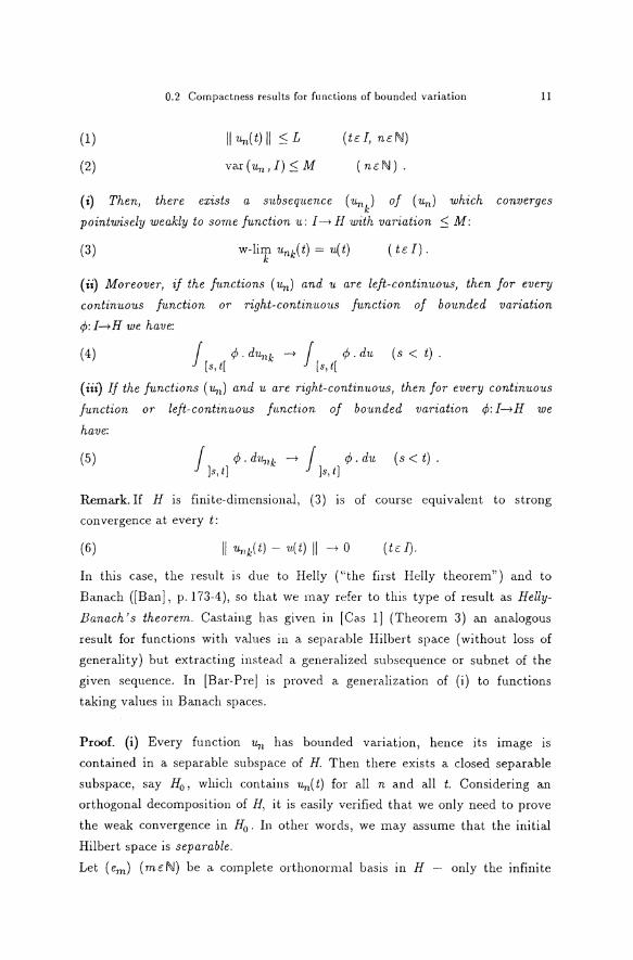
(1)

(2)

0.2 Compactness results for functions of bounded variation

II ~Ln( t) II :::; L (tc: I, nc:N)

(nc:N).

11

( i) Then, there exists a subseqnence ("u11 ) of ("u11 ) which converges k

pointwisely weakly to sorne function u: I-> H with variation :::; M:

(3) w-lim Unk( t) = ·u( t) k

(tc:I).

( ii) M oreover, if the j1mctions ( u11 ) and u are left-continuous, then for every

continuous function or right-contin-u.ous function of bounded variation

cp: I->H we have:

(4) J cp.dun/,;-> j cp.du (s < t). [ s, t[ [ s, t[

( iii) Ij the functions ( u11 ) and u are right-continuous, then for every continuous

function or left-continuous fnnction of bo·unded variation cp: I->H we

have:

(5) J cp . d1t11 k -> j cp . du ( s < t) . Js, t] ]s, t]

Remark. If H is finite-dimensional, (3) is of course equivalent to strong

con vergence at every t:

(6) II U 11 J,;( t) - 1l( t) II -> 0 (tc: I).

In this case, the result is due to Helly ( "the first Helly theorem") and to

Banach ((Ban], p. 173-4), so that we may refer to this type of result as Helly­

Banach 's theorern. Castaing has given in [ Cas 1] (Theorem 3) an analogous

result for functions with values in a separahle Hilbert space ( without loss of

generality) but extracting instea.cl a generalized subsequence or subnet of the

given sequence. In (Bar-Pre] is proved a generalization of (i) to functions

taking values in Banach spaces.

Proof. (i) Every function u11 has bouncled variation, hence its image is

contained in a separable subspace of H. Then there exists a closed separable

subspace, say H0 , which contains 1t11 ( t) for all n and all t. Considering an

orthogonal decomposition of H, it is easily verified that we only need to prove

the weak convergence in H0 . In other worcls, we may assume that the initial

Hilbert space is separable.

Let ( em) ( rnc: N) be a complete orthonormal basis in H - only the infinite

12 Chnpt.cr 0: Preliminaries

dimensional case, not treated in [Ban] , interests us here. For every m, the real

functions ttn( t) . em ( n c: N) a.re uniformly bounded by L and uniformly

bounded in variation by M.

Banach' s result, as mentioned above, implies that there is a subsequence j 1

suchthat ttn(t). e1 (for ttnc:j 1) converges everywhere to a bv function fr(t); and then there exists a subsequence 12 of 11 such that u71 ( t) . e2 converges

pointwisely to a bv function h( t) a.long 12 ; and so on. The classical

diagonalization procedure furnishes in this manner a subsequence (Unk) of ( ttn) for which

1tnk( t) · em ---+ !,11( t),

where Um) is a sequence of bv functions from I to IR.

For every t in I, T(h) := limk ·tt11k(t) . h. defines a continuous linear functional

on H, with T{ em) = !,11 ( t) and I T( h.) I :::; L II hll . By Riesz representation

theorem, there is a unique ·u.(t)t:H such tha.t T(h)=u(t).h holds for every

hc: H. Then ( u11k) converges pointwisely weakly to this function u: I---+ H. Moreover, u has bounded va.ria.tion. In fact, given any choice of nodes in I, we

have, by the lower semicontinuity of the norm in the weak topology of H:

p

< lim L llunk(t;)- '1L11 k(ti-l) II :::; lim var(u71k 1 I):::; M, i-')

whence var( u; I) :::; M.

(ii) We assume that ~ is continuous or tha.t ~ is right-continuous and of

bounded variation. Given any f > 0 let us take a partition Ji = [si 1 si+1[ of

J= [s1 t[ (with i=O, ... , m) such tha.t the oscillation of ~in every subinterval

IS not greater than f. The right-continuous step-function 1/J, defined

by 1/J( T) : = ~ ( si) ifT c: Ji , sa.tisfies II V'- <P II = :::; f and

J ·lj;. dunk = L </>(sj) . j du11k . 1 0~1~m [si• 5 i+1[

Because the functions ~~ and u are left-continuous and by (3), we have:

lim j k [si,si+l[

and so

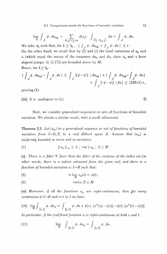
0.2 Compactness results for funct.ions of bounded variation 13

lim j 1); . dunk = L </;( si) . j du = j 1); . du. k J o::;z::;m [si• 5i+l[ J

We take ko such that, for k ?: ko , I I J 1);. dunk - I J 1); · du I :S € ·

On the other hand, we recall that by (2) and (i) the total variations of Un and

u (which equal the norms of the measures dun and du, since u11 and u have

aligned jumps; cf. (1.17)) are bounded above by M.

Hence, for k ?: ko :

I j J </; . dunk- j J </; • du I :<::; j J II <P -1); II I dunk I + I j J 1); . dunk- j J 1);. du I + j J 111);-<f; 111 du! :S (2M+l) €,

proving (4).

(iii) It is analogaus to (ii). 0

Next, we consider genera.lized sequences or nets of functions of bounded

variation. We obtain a similar result, with a small refinement.

Theorem 2.2. Let ( ua) be a gen.eralized seqnen.ce or n.et of function.s of bounded

variation from I=[O, T] to a real Hilbert space H. Assurne that (ua) is

uniformly bounded in norm a.nd ·in 1Ja.riu.tion:

(7) II 'Ilex !I 00 :<::; L ; var ( 'Ua ; I) :<::; M .

( i) There is a filter '3' finer tlwn the filtcr of thc sections of the index set (in

other words, there is a subnet extracted from the given net) and there is a

function of bounded variat-ion u: I-+H such that:

(8)

(9)

w-lim 1/.c;(t) = ·u(t), "J

var(u;IJ :<::; M.

(ii) Moreover, if all the fv.nctions ·u0 a.re right-continuous, then for every

continuous <f;: I-+H and s<t in I we have:

(10) limj </;. dua = j q>. d1L + <f;(s). [v+(s) -1L(s)]- <f;(t). [u+(t)- u(t)]. <J ]s, t] Js, t]

In particular, if the (sub )Iimit function n is right-cont·inuous at both s and t:

(11) lim <J

j </; . d1Ln = j </; . du . ]s, I] ]s, I]

14 Chapter 0: Preliminaries

Proof. (i) Since the net is uniformly bounded and balls are weakly compact in

H, it follows from Tychonoff's theorem that ( u0 ) is relatively compact in the

topology of pointwise weak convergence. Thus, there exist '?J and u satisfying

(8). lnequality (9) is obtained as in the preceding theorem.

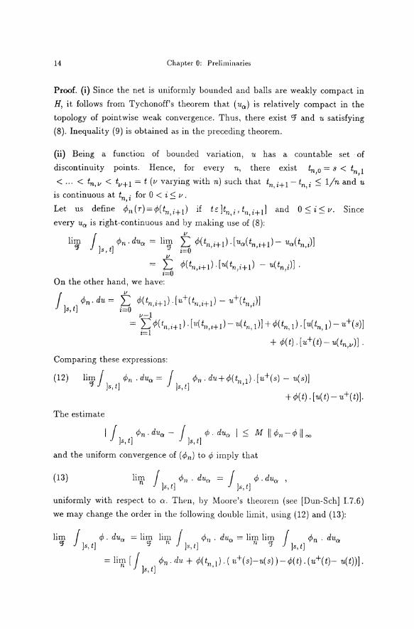
(ii) Being a function of bounded variation, u has a countable set · of

discontinuity points. Hence, for every n, there exist ln,o = s < tn,l

< ... < tn,v < tv+ 1 = t (v varying with n) suchthat tn,i+l- tn,i :=:; 1/n and u is continuous at tn, i for 0 < i :=:; 11 •

Let us define cPn(r)=cf;(tn,i+1) if tc:Jtn,i,tn,i+d and O:S:i:S:v. Since

every u0 is right-continuous and by making use of (8):

!im j cPn. dua = !im t cf;( tn i+1). [ ua( tn i+1)- ua( tn i)] ~ ]s, t] ~ i=O ' ' '

V

= L cf;(tn,i+l) · [u(tn,i+1) - u(tn)J · i=O

On the other hand, we have:

J cPn·du= t cf;(tni+1).[·u+(tni+l)-u+(tni)J ]s, t] i=O ' ' '

v-1 = 2:cf;(t1l i+l).[11.(tn t+rJ-u(tn rll+cf;(tn rl-[u(tn 1)-u+(sJJ

i=l J ' ' , '

+ cf;(t).[u+(t)-u(tn,v)J.

Comparing these expressions:

(12) limj c/; 71 .du0 = J cPn·du+cf;(t111 ).[u+(s)-u(s)] ~ ]s, t] ]s, t] '

+ cf;( t). [ u( t)- u+(t)].

The estimate

I j cPn · dua - J cP · dua I :S: M II <Pn- cf;JI = ]s, t] ]s, t]

and the uniform convergence of ( <Pn) to <P imply that

(13) liW j <Pn . dua = j <P . du-a , ]s, t] ]s, t]

uniformly with respect to o:. Then, hy Moore's theorem (see [Dun-Sch] 1.7.6)

we may change the order in the following double Iimit, using (12) and (13):

!im j cf; . dua = !im !im j c/; 11 • dua = !im !im j <Pn . dua ~ ]s,t] ~ 71 Js,t] 11 ~ ]s,t]

=!im rj <Pn.d"U. + cf;(tn 1).(u+(s)-·n(s))-cf;(t).(1t+(t)- u(t))]. n ]s, t] '

0 .. 3 Convergence in the sense of fillecl-in graphs 15

To conclude it suffices to rema.rk that c/;(tn 1)----* c/;(s), because c/; is continuous '

and I tn,l- s I :::; 1/n, and that J ]s, t] !/in. dn----* J ]s, t] <P. du is obtained in the

same way as (13). D

We leave it to the reader to formulate and prove the analogue of (ii) for

functions of bounded variation which are left-continuous.

0.3. Convergence in the sense of filled-in graphs In this section, we introcluce a notion of convergence which seems well-aclapted

to the stucly of cliscontinuous functions, by provicling a reasonable substitute

for uniform convergence. In view of the applications we have in mind, we shall

restriet ourselves to consiclering right-continuous functions of bounded

variation, rcbv funct·ions for short.

Let f: I ---> H be an rcbv function from a real interval I= [0, T] to a

Hilbert space H. W e define the Jillcd-in graph gr* f by aclcling, if necessary,

some line segments to the graph of f in such a way that all its gaps, if any, are

filled. To be precise,

gr* != { (t, x): 0:::; t :::; T ancl XE [ r(t), fit)]}'

where [y, z] stands for the line segment between two points in H ancl J-(t) is

the left limit of f at point t. Here, by convention, f-(0) = f( 0).

Fillecl-in graphs of snch rcbv functions are closed bounclecl suhsets of

the procluct space I x H; hence, we may consicler the Hausclorff distance

between any two of them with respect to a suitable metric, for instance,

b ((t,x),(s,y)) = max {I t-s I, II x-y II }.

Recall that in a metric space ( X, b ) the Hausdorff distance between

two (non-empty closecl) subsets A ancl Bis clefinecl by

h(A,B)=max{ e(A,B), e(B,A)},

where e ( A, B) is the excess or separation of A from B which is given by

e(A,B) = sup { clist( a, B): at:A} = sup inf b( a, b). at:A beB

If fand gare two rcbv functions, we clefine

h*(f,g) := h(gr·* f, gr* g),

16 Chapter 0: Prelimi11aries

that is, the Hausdorff clistance between their filled -in graphs with respect to

the metric 8 introduced above. This is a metric in rcbv( I, H), because of the

general properties of Hausclorff distances a.ncl of the following:

Proposition 3.1. IJ f and g are rcbv fnnctions such that h *(J, g)

f=g.

0, then

Proof. Suppose, by contradiction, that f{f-o) 1- g(ta) for some ta in (O,T(. Since

both functions are right-continuous, there is t > 0 such that if both t and s

belong to 1= ]ta, ta+t[, then llfi.t)-fi.ta) II < 8 and llg(s)-g(ta) II < 8 where

8 = II J( ta)- g( ta) II /3. It follows that II g-( s)- g( ta) II :S: 8. Hence, if ( s, x) c gr* g

with sc J, i. e., Xe [g-(s), g(s)], then II x- g(ta) II :S: 8 ; so that II x- J(t) II 2: 8,

for every t in J. Let t1 = ta + t/2. If ( s, x) belongs to the filled-in graph of g,

then either s~J and so ls-t1 1 2:t/2; or scl ancl then llx-f{t1)11 2:8. We

conclude that

h*(J,g) 2: dist((t1, fi.t 1)), gr*g) 2: min { t/2, 8} > 0,

which contradicts the initial hypothcsis.

We have shown so far that f= g on [0, T[, which also implies J-( T) = g-( T).

Suppose that f is left-continuous at T. Since clist (( T, g( T)), gr*J) = 0 , by

hypothesis, then there exist sequences tn-'> T and Xn c u-(tn), fi. tn)l with

x71 -'> g( T). Both f-(t71 ) and fi. t71 ) converge to J-( T) = fi. T), ancl this forces x71

to do the same. Hence J( T) = g( T); in particular, g is also left-continuous at T.

Finally, we suppose that f and g are both cliscontinuous at T. Let

x c ]f-(T), fi.T)] (in an obvious sense) a.ncl consider a sequence (t71 , x71 ) in gr*g

which converges to ( T, x). Then t11 = T for all n !arge enough, otherwise x71

would converge to f-(T) 1- x. Hence x71 belongs to [g-(T), g(T)] and so does

the Iimit x. From the previous considerations and exchanging the roles of fand

g we infer that line segments [r(T), fi.T)] ancl (g-(T), g(T)] = [r(T),g(T)]

are the same, whence fi. T) = g( T). 0

The next simple result relates convergence m the sense of filled-in

graphs with uniform convergence.

Proposition 3.2. If f and g are rcbv functions, then

(1) h.*U, g) ::::: II f- g II oo .

Thus, every sequence of rcbv functions wh.ich converges un·iformly to an rcbv

function also converges in the sense of filled-in graphs to the same function.

0.3 Convergence in the sense of fillecl-in graphs 17

Proof. Let r= II f- g II 00 , the sup norm. For every t in I, II ./( t)- g( t) II :S r.

Since the same is true for every s < t, we ha.ve II f-( t)- g( t) II < r. Hence:

h( [r(t),j(t)] 1 [g-(t), g(t)]) :::; T' 1

with respect to the norm metric of H a.ncl ( 1) follows ea.sily. D

This notion of convergence of filled-in gra.phs presents an inconvenient

feature, already detected for the convergence of graphs, as introduced by

Moreau [Mor 4]: a sequence of filled-in gra.phs ma.y converge in I x H, in the

sense of Hausdorff distance, to a. limit set L without L being the filled-in graph

of an rcbv function.

The followiilg example shows tltis a.nd also makes it clear that, in

genera.l, from a sequence of rcbv functions, which are uniformly bounded both

in norm and in variation, it is not possible to extra.ct a. subsequence which

converges in the sense of filled-in graphs to an rcbv (or simply bv) function,

even if the functions ta.ke their va.lues in a. finite dimensional spa.ce.

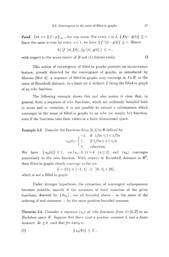
Example 3.3. Consicler the functions from [0, 1] to IR defined by

-1 if lj3n :S t < 1/2n

u11 (t)= { 1, ' if 1/2n :S t < 1/n

0, othcrwise.

We have llu.11(t)ll :S1, var(n11 ; 0,1)=4 (n~2} ancl (u11 ) converges

pointwisely to the zero function. \Vith respect to Hausdorff distance in IR2,

their fillecl-in gra.phs clearly converge to the sct

L={O}x[-1,1] U ]0,1]x{O},

which is not a filled-in graph.

Under stronger hypotheses the extraction of convergent subsequences

becomes possible, namely if the mea.sures of total va.ria.tion of the given

functions, denoted by I d·u11 I , a.re a.ll houncled above - in the sense of the

ordering of real measures - by the same positive bounded mea.sure.

Theorem 3.4. Cons·ider a seqnence ('u. 11 ) of rcbv fu.nctions from. I=[O,T] to an

Euclidian space E. Suppose that there cxist a positive constant L and a finite

measure dv ~ 0 such that for eue7"!J n:

(2) 111tn(O) II < L ,

18

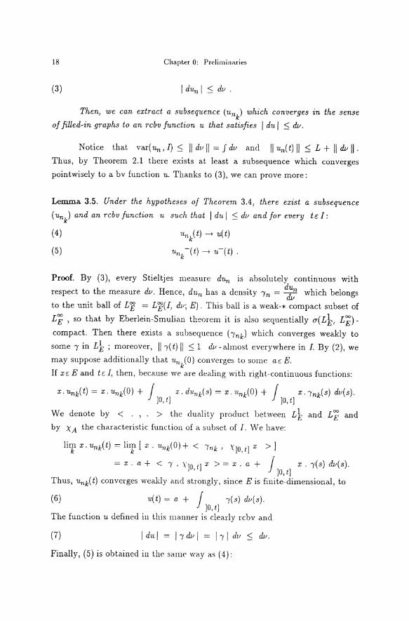
(3)

Chapter 0: Preliminaries

Then, we can extract a subsequence (u 11 ) which converges in the sense k

of filled-in graphs to an rcbv function u that satisfies I du I S: dv.

Notice that var( un, I) S: Jl dz; II = f dv and II Un( t) II S: L + II dv II . Thus, by Theorem 2.1 there exists at least a subsequence which converges

pointwisely to a bv function u. Tha.nks to (3), we can prove more:

Lemma. 3.5. Under the hypotheses of Theorem 3.4, there exist a subsequence

( Un ) and an rcbv function 11. su.ch that I dn I S: dz; and for every t c: I: k

(4)

(5)

·n11k(t)-> u(t)

1t11 -(t)-> u-(t) . k

Proof. By (3), every Stieltjes mea.sure du11 is a.bsolutely continuous with

respect to the measure dv. Hence, dun has a density ln = dd~1 which belongs

to the unit ball of LE = LE(I, dl!; E). This ball is a weak-* compact subset of

L';; , so that by Eberlein-Smulia.n theorem it is also sequentially a( Lb, L';;)­compact. Then there exists a subsequence ( lnk) which converges weakly to

some 1 in Lk ; moreover, Jll( t) II S: 1 dz;- almost everywhere in I. By (2), we may suppose additionally that Un (0) converges to some aE E.

k If xc: E and tc I, then, because we are dealing with right-continuous functions:

x.u11 k(t) = x.u11 k(O) + j x.du71 k(s) = X.1t71 k(O) + j X·lnk(s) dz;(s). ]0, I] ]0, I]

We derrote by < . , . > the clua.lity product between L} and L';; and by XA the characteristic function of a subset of I. We have:

lim x.u11 k(t) = lim [ x. ·u.11 k(0)+ < lnk, X]o I] x >] k k ,

= x. a + < ~I , X]o t] x > = x . a + j x. 1(s) dv(s). , . ]0, t]

Thus, unk( t) converges weakly and strongly, since Eis finite-dimensional, to

(6) u.(t) = a + j 1(s) dz;(s). ]0, t]

The function u defined in this manner is clearly rcbv and

(7) I d·u I = l1 dz; I = II I dz; < dz;.

Finally, (5) is obta.inecl in the same way as (4):

0.3 Convergence in t!Je sense of Ii IIed-in graphs

lim x.unk-(t) =lim[x.u11k(O)+ j X·ink(s)dv(s)] k k ]0, t[

= x . [ a + j 1( s) dll( s) J = x . u- ( t) . ]01 t[

This section ends with the:

19

0

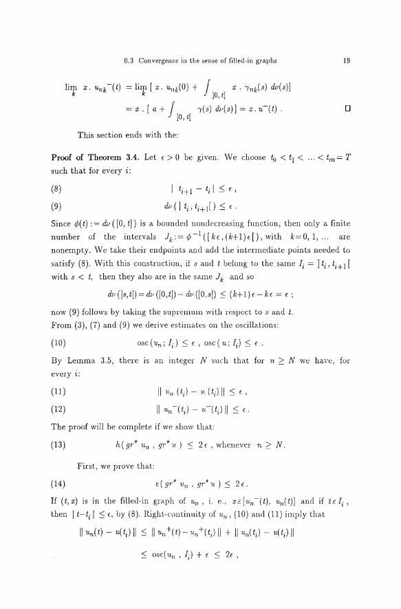
Proof of Theorem 3.4. Let E > 0 be gi ven. W e choose lo < t1 < ... < tm = T

such that for every i:

(8)

(9)

I t;+ 1 - t; I :::; " ,

dll ( l t; I ti +I [ ) :::; t .

Since <fJ(t): = dv ( [01 t]) is a bounclecl nonclecreasing function, then only a finite

number of the intervals Jk:=<P-1 ([kt,(k+1)f[),with k=0,1, ... are

nonempty. We take their endpoints and adcl the intermediate points neecled to

satisfy (8). With this construction, if s ancl t belang to the same I; = ] t; 1 ti+ 1 [

with s < t, then they also are in the same Jk and so

diJ(]s 1 t])=di/([0 1 tj)-diJ([O,s]):::; (k+1)c-kc = E;

now (9) follows by taking the supremnm wit!J respect to s ancl t.

From (3), (7) and (9) we derive estimates on the oscillations:

(10)

By Lemma 3.5, there is an integer N such that for n 2:: N we haYe, for

every i:

(11)

(12)

II 11" ( t;) - ·u ( t; J II :::; c ,

II un-(t;l - u-(t;) II :::; c.

The proof will be complete if we show that:

(13) h(gr* u11 , gr*·u.) :::; 2c, whenever n 2:: N.

First, we prove that:

(14) e ( gr * 11.71 , gr * 1L ) :::; 2 E •

If (t1 x) is in the fillecl-in graph of 1L11 , i. e., xE: [11.11-(t) 1 11.n(t)] and if t;: I;,

then I t-t; I :::; E, by (8). Right-contirmity of 11.11 , (10) and (11) imply that

II u11 ( t) - u( t;) II < ll1t71 +( t)- u,/( t;) II + 111t11 ( t;) - u( t;) II

< osc( u11 , I;) + c :::; 2c ,

20 Chapter 0: Preliminaries

and analogously II Un -( t)- u( t;) II S 2E. This implies II x- u( t;) II S 2 E and so

dist( ( t,x), gr*u) :S b ( ( t,x), ( t;, v.( t;))) :S max { E, 2E'} = 2E .

If t is one of the points t;, then x belongs to the segment ( un -( t;), un( t;)] whose

Hausdorff distance in E to [u-(t;), u(t;)] is not greater than €, by (11)

and (12). It follows easily that

dist((t;,x),gr*u) :S dist((t;,x),{t;} x [u-(t;),u(t;)]) :S ~:,

thus ending the proof of (14 ).

We conclude by proving that, symetrically:

(15) e ( gr* u , gr* v.n ) S 2 €.

If ( t;, x) E gr* u, then as above:

dist ( (t;, x), gr*un) S dist ( (t;, x), {ti} X [ Un -(t;), un(t;)])

S h( [ tt-(t;), ·u.(t;)], [un-(t;), un(t;)]) S E.

If tc I; and x E [u-(t), u(t)], then I t- t; I < E and

II u- ( t)-un(t;) II S II u- ( t)-u+(tJ II + II u( t;)-un( t;) II S osc( u; I) + E S 2E.

Similarly, II u( t)- un( t;) II S 2 E.

D

0.4. Geometrical inequalities The first inequality presentecl here concerns the Hausdorff clistance h between

subsets of a Hilbert space H. It implies that if a continuous rectifiable arc l has

length not much greater than that of a certain line segment and if the

respective endpoints are not very far apart, then the Ha.usdorff distance

between arc a.nd segment is small. We clo not a.im at giving the optimal

quantification of this property.

Lemma 4.1. Let [x1 , ~] be a line segment in H. Let l be a continuous

rectifiable arc with length lll not greater than II x1-~ II + 11 and with

endpoints y1 and Y2 such that II Y1- xl II S b and II Y2- ~ II S T). Here v, b

and T) are nonnegative numbers s·u.ch that v+b+ry :S 1. Then

(1)

0.4 Geometrie~] inequalities 2I

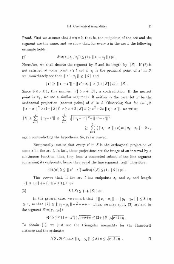
Proof. First we assume that b = TJ = 0, that is, the endpoints of the arc and the

segment are the same, and we show that, for every z in the arc l, the following

estimate holds:

(2)

Hereafter, we shall denote the segment by S and its length by I SI . If (2) is

not satisfied at some point z 'c; l ancl if xi is the proximal point of z' in S,

we immediately see that II z '- x2 II ~ I SI and

Since 0:::; v:::; 1, this implies 111 >I/+ I SI , a contracliction. If the nearest

point is x2 , we use a similar argument. If neither is the case, Iet x' be the

orthogonal projection (nearest point) of z' in S. Observing that for i= 1, 2

II z'- x' 11 2 > (1+ I SI )2 r; ~ v + 2 I SIr; ~ r;2 + 2r; II xi- x 'II , we write:

2 ~ L ( II xi-x'll +v)= II xi-~ II +2v,

i=I

again contradicting the hypothcsis. So, (2) is proved.

Reciprocally, notice that every x' in S is the orthogonal projection of

some z' in the arc I. In fad, these projections are the ima.ge of an interva.l by a

continuous function; thus, they form a connected subset of the line segrnent

containing its endpoints, hence they equal the line scgment itself. Therefore,

dist(x', l):::; II x'- z'll =dist(z',S)::::; (1+ I SI )\[V.

This proves that, if the arc l has enclpoints x1 and ~ and length

lll < ISI+v(O::::;r;::::;1),then:

(3) h( l, S) ::::; ( 1+ I s I ) \[17 .

In the generat case, we remark that I II x1 - ~ II - II Y1- Y2ll I ::::; b + TJ

::::; 1, so that 111 ::::; II y1 - y2 II + b + TJ + 11. Thus, we may apply (3) to land to

the segment S '= [yl, Y2J :

h(l, S')::::; (1 +I S'l )~v+O+ry::::; (2+ I SI )~v+O+ry.

To obtain (1 ), we just use the triangular inequality for the Hausdorff

distance and the estimate:

h(S', S)::::; max II xi- Yi II ::::; O+ry::::; ~v+O+ry 0

22 Chapt.er 0: PrelimiuRrics

The next set of results, by l\1oreau and Valadier, is essential in order to

estimate the variation of the solutions to a new dass of sweeping processes.

Lemma 4.2. [Mor 8] Let S be a contraction from a subset D of a Hilbert space

into itself. Assurne that P, the set of fixed points of S, contains some

closed ball B( a, r) , r > 0. Then, for euery x c: D, we have:

(4)

Proof. Let y be such that II y II = 1 ancl x- S(x) = II x- S(x) II y. Since a+ ryc: P

and since S is a contraction, it follows that II a+ ry- x 11 2 2 II a.+ ry- S(x) 11 2 ,

i. e.,

Then,

i r ( II x- a II 2 - II S( x) - a II 2) 2 y . ( x - S( x)) = II x - S( x) II . 0

An easy consequence of Lt>mma. 4.2 is:

Lemma 4.3. In a Hilbert space H, we cons·ider a closed convex set C which

contains a closed ball B( a, r) ( r > 0) . Let u H Then:

(5) II x- proj(x, C) II ::; d-1• ( 1/1:- a f - II proj(x, C)- a 11 2 ) .

Proof. [Val 2] It suffices to apply the prececling Iemma to the projection of best

approximation on C, S(x):= proj(x, C) (st>e p. 26). In fact, S is a contraction

of H having C as set of fixecl points. 0

For iterative proceclures we may use the following estimates.

Lemma 4.4. Let C1 , ... , C" be closed con·uex subsets of H all of them

containing a fixed closed ball B( a, r) ( r > 0). If Xo c: H and if x1 , ... , Xn are

defined inductively by xi=proj(xi-l, C;), then:

(6)

(7)

Proof. [Val 2] Inequalities (6), which hold even if r=O, result from the fact

0.4 Geomctrical inequalities

that projections are contractions:

llx1-all = llproj(Xo,C1)-proj(a,Cl)ll < IIXo-all

and so on.

Since C; :::) B( a, r) , then by the preceding Iemma we know that

llx;-xi-111 ~ 21r(11xi-l-all 2 -llx;-all 2 )

for i= 1, ... , n; adding up these inequalities we obtain (7).

R.emarks.

1) Tobemore precise, we can prove that ([Val 2])

n 1 2 ? (8) ~ II x;- xi-1ll ~ max { 0, 2r ( II Xo- all -r")} ·

z=l

23

0

In fact, either II Xo- a II ~ r ancl then X;= Xo for every i, so that (8) is trivial;

or II Xo- a II > r ancl it is easily verified tha.t II x71 - a II 2': r, hence (8) follows

from (7).

Notice that

is the length of the arc of the "developpante" of the circle with radius r

( centered at a) lying between this circle a.ncl the circle of radius II Xo- a II ( this is a curve drawn by the end of a rigid bar rolling without sliding on a circle

with radius r). It was under this form tha.t Valadier initially stated the

property (see [Cas 1] appendix ancl [Val1]). His first proof, although more

complicated, is nevertheless still interesting because of the underlying intuitive

geometrical consiclerations. If H =IR, a better estimate is given in [Val 2].

2) This type of inequality had alreacly been used by Moreau in [Mor 9] ((5.2),

p. 31) and [Mor 8] (remark 2, p.l44). In the former, the sweeping process by a convex set having bouncled but not necessarily continuous variation and containing the ball B( a, r) is consiclered; it is shown that the total variation of the solution is bounded above by II x0 - a 11 2 /r, where Xo is the initial value. In

the latter, which concerns the sweeping process by a convex set with

absolutely continuous variation, it is provecl that the absolutely continuous

solution u satisfies a. e.

II du II < - l.. ..4 II a- u 11 2 · dt - 2r dt ' by integration, this yielcls an estimate ecptiva.lent to (7):

24 Chapter 0: Preliminaries

v ar( u; 0, T) ::; 2\ ( II a - u( 0) II 2 - II a - u( T) II 2 ) .

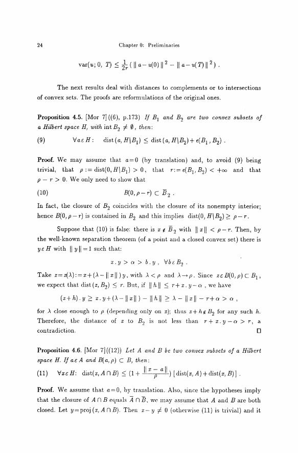
The next results deal with distances to complements or to intersections

of convex sets. The proofs are reformulations of the original ones.

Proposition 4.5. [Mor 7] ((6), p.173) IJ B1 and B2 are two convex subsets of

a Hilbert space H, with int B2 I- 0, then:

Proof. We may assume that a=O (by translation) and, to avoid (9) being

trivial, that p := dist(O, H\B1) > 0, that r:= e(B1, B2) < +oo and that

p - r > 0. We only need to show that

(10) B(O,p-r)cB 2 .

In fact, the closure of B2 coincides with the closure of its nonempty interior;

hence B(O,p-r) is contained in B2 and this implies dist(O,H\B2)::::: p-r.

Suppose that (10) is false: there is x ~ B 2 with II x II < p- r. Then, by

the well-known separation theorem ( of a point and a closed convex set) there is

yc H with II y II = 1 such that:

Take z=z(>-):=x+(>--llxll)y,with A<p and A-->p. Since zcB(O,p)CB1 ,

we expect that dist (z, B2) ::; T. But, if II h II ::; r+ x. y- a , we have

(z+ h). y ::::: x. y+ (A -II x II)- II h II ::::: A- II x II - r+ a > a ,

for ). close enough to p (clepencling only on x); thus z+ h'lc B2 for any such h.

Therefore, the distance of z to B2 is not less than r + x. y - a > r, a

con tradiction. 0

Proposition 4.6. [Mor 7]((12)) Let A and B be two convex subsets of a Hilbert

space H. IJ ac A and B( a, p) C B, then:

(11) Vxc H: dist(x, An B) :::: (1 + II X; a II) [ dist(x, A) + dist(x, B) J .

Proof. We assume that a=O, hy translation. Also, since the hypotheses imply

that the closure of A n B equals A n B, we may assume that A and B are both

closed. Let y=proj(x,AnB). Then x-y I- 0 (otherwise (11) is trivial) and it

0.4 Geollletrical inequalities 25

belongs to the outwa.rd normal cone to An B at y. Under our assumptions on

a, this cone is the sum of the two normal cones to A ancl B. Usual notations

for the outward normal cone are NA(y) or ()1j.JA(y), the subdifferential of the

indicator function 1/J A ( x) = 0, if XE A ancl + oo otherwise. A well-known result

from Convex Analysis implies that:

o!jJ A n B = 8( 1/J A + 1/J B) = o'lj; A + o'lj; B ,

since both indicator functions are finite at a, one being continuous. Hence,

x-y = p+q , pt:NA(y), qt:NB(Y).

If p = 0, then y = proj ( x, B), clist ( x, An B) = clist ( x, B) ancl (11) is trivial.

Similar remark if q=O. Take ·u= II x- vll-l p ancl v= II x- vll-l q so that

x-y= llx-vll (u+v), llu+vll =1. Since ut:NA(y) and Ot:A, we have

u. (y- 0) 2: 0; ancl ·vt: N8 (y), B(O, p) C B imply that

·v.(y- Pwl:::: o. Hence:

(12) u. y 2: 0 , ·v. y 2: p II v II

We show that:

(13) (x- y).u::; llu-11 dist(x,A).

In fact, A is contained in the half-space H(A) = { z: (z- y). u ::; 0} and the

projection of x in H( A) is z: = x - ,\ 11, where ,\: = ll1t 11-2 ( x - y) . 1L is positive

(otherwise (13) is trivial). Hence, dist(l:, A) 2: II x- z II and (13) follows,

because II x - z II = ,\ llu II = I Iu II -l ( x - y) . u .

implies

Similarly, ( x - y) . ·v ::; II u II dist( x, B) . Then

dist(x,AnB)= llx- Yll =(x- y). (u+v)

(14) clist(x, An B) ::; 111t II clist(x, A) + II VII clist(x, B) ,

and also, in view of (12),

0 ::; clist( X, An B) ::; X. ( u + v) - y. V ::; II XII - p II VII . Thus:

II v II ::; J4lL , II u II ::; 1 + II ·u II ::; 1 + II ; II , so that the result follows from ( 14 ). D

26 Chapter 0: Preliminaries

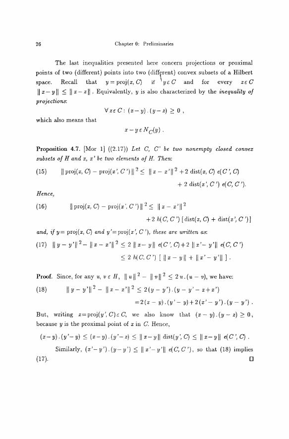
The last inequalities presentecl here concern projections or proximal

points of two (different) points iJ.1to two ( diffrent) convex subsets of a Hilbert

space. Recall that y = proJ(X, C) if yc C and for every zt: C

II x- y II ~ II x- z II . Equivalently, y is also characterized by the inequality of

projections:

'</zcC: (x-y).(y-z) ~ 0,

which also means that

X -y~::Nc(y).

Proposition 4.7. [Mor 1] ((2.17)) Let C, C' be two nonempty closed convex

subsets of Hand x, x' be two elements of H. Then:

(15) II proj(x, C)- proj(x', C ') 11 2 ~ II x- x'll 2 +2 dist(x, C) e(C ', C)

+ 2 dist(x', C') e(C, C').

Hence,

(16) II proj(x, C)- proj(x', C ') 11 2 :S II x- x'll 2

+ 2 h( C, C ') [ dist( x, C) + dist( x ', C ')]

and, ify= proj(x, C) and y'=proj(x', C'), these are wrdten as:

(17) IIY- y'll 2-llx- x'll 2 ~ 2llx- Yll e(C',C)+2IIx'- y'll e(C,C')

::; 2 h( C, c ') [ II X - y II + II X'- y 'II l .

2 •J Proof. Since, for any u, v c H, II u II - II v 11- ~ 21t. ('u- v), we have:

(18) !!y-y'll 2 -llx-x'!l 2 ~2(y-y').(y-y'-x+x')

=2(x- y).(y'- y)+2(x'- y').(y- y').

But, writing z=proj(y', C)t: C, we also know that (x- y). (y- z) ~ 0,

because y is the proximal point of x in C. Hence,

(x-y).(y'-y) :S (x-y).(y'-z) :S llx-yll clist(y',C)::; llx-yll e(C',C).

Similarly, (x'- y'). (y- y') ~ II x'- y'll e(C, C '), so that (18) implies

(17). 0

Chapter 1

Regularization and Graph Approximation of a Discontinuous Evolution

1.1. Introduction Moreau has shown that a Yosida-type regularization procedure can be used in

order to prove the existence of a solution to the so-called sweeping process or

evolution problem associatecl with a. moving convex set (see e.g. [Mor 3]). If

this set is supposecl to be Lipschitz-continuous in the sense of Ha.usdorff

dista.nce, then the solution to the problem it defines is also Lipschitz­

continuous with respect to a real variable t. The Yosida or Moreau-Yosida

a.pproximants, that is, the absolutely continuous solutions to the regularized

differential equations clerivecl from the initial problem, then converge

uniformly to the solution to the sweeping process.

If we try to carry out a similar program for a cliscontinuous evolution,

say one that is determined by a convex set with bouncled variation, it is clear

that uniform convergence is not to be expected since the Iimit solution is not

necessarily a continuous function. Insteacl, a reasonable substitute is found in

the concept of graph convergence, to be precise, convergence of filled-in graphs

with respcct to Hausdorff clistance (§0.3). In this way, we account for

uncertainties both in the values and in thc arguments of the concerned

functions, a feature that will certainly appea.l to the numcrical ana.lyst.

We present here the genera.l resnlt concerning evolutions in arbitrary

Hilbert spaces, which appea.recl in [Mon 5] - a previous preprint version dealt

only with the finite-dimensional case. Notice the additional compactness

hypothesis on the moving convex set, not needed in Moreau's theory (even for

Yosida approximation of an absolutely continnous evolution, [Mor 3], § 5.g).

Example 1.3 below also shows that we cannot extend the results to

multifunctions with right-continuous retraction.

Let H be a real Hilbert space with scalar product denoted by a dot and

I be a compact interval [0, T] of the real line. We consider a multifunction

(that is, a set-valued function) C: t --t C( t) from I to nonempty closed convex

subsets of H. This multifunction, also referrecl as C(.) or C, can be interpreted

28 Chapter 1: Regularization and Graph Approximation of a Discontinuous Evolution

as describing the evolution of a convex "mobile" (moving set) between the

instants t = 0 and t = T. We suppose that Cis of bounded variation and right­

continuous, rcbv for short; this means that its variation function v(.) is right­

continuous and finite on I. For our purposes, it 1s enough

to recall that v( t): = var ( C; 0, t) is nondecreasing and satisfies

(I) h(C(s),C(t))~v(t)-v(s) (O~s~t),

where the h refers to Hausdorff distance between subsets of H, with respect to

the norm metric.

Definition 1.1. A right-continuous function of bounded variation w: I --t His a

solution to the sweeping process by the convex moving set C(.) with initial

value ac: C(O) if it satisfies the following conditions:

(2)

(3)

w(O) = a;

w(t) c:C(t) (tel);

and there exists a positive measure dp. on I relative to which the Stieltjes

measure dw of w has a density ul c: L1(I, dp.; H) , i. e., dw = ul dp., such that :

(4) -ul(t)c: NC(t) (w(t)), for d1t-almost every t in I.

This is written shortly as:

(5) -dw c: NC(t) (w(t)).

We propose to approximate the solution to this differential inclusion,

which is known to exist and to be unique [Mor 1], by solutions to suitable

differential equations.

Definition 1.2. Given .A>O, the respective Yosida approximant is the unique absolutely continuous solution to the Cauchy problem:

(6)

(7)

d:/' (t) + ± [ 1LA(t)- proj ( v.A(t), C(t))]

·uA(O) = a,

O· '

where (6) is to be satisfied by almost every t in I, in the sense of Lebesgue

measure. In (6), proj(x, C(t)) clenotes the point of C(t) which is closest to x,

usually called the projection or the proximal point of x in C( t).

1.1 lntroduction 29

As we have remarked already, in general the Y osida approximants do

not converge uniformly to the solution w of the sweeping process, when ..\--> 0;

in fact, they are continuous and w is possibly discontinuous. We illustrate this

with two simple examples. First, we recall that a function r is a retraction

function, or better said a "super-retraction" of a multifunction C if the excess

of C( s) with respect to C( t) satisfies

e(C(s),C(t))::::; r(t) -1·(s), Vs::::; t.

Example 1.3. Let H =IR and define C on the interval I= [0,2] :

C(t)=[0,2] ift:f1; C(1)=[1,2].

Then C has right-continuous retraction: r( t) = 0, for t < 1 and r( t) = 1 for

t 2: 1. Take a = 0 as initial value. It is easily seen that u). = 0 for any ..\>0,

while the solution to the sweeping process is w( t) = 0, if t < 1, and w( t) = 1, if

t 2: 1 . In this case, there is no convergence of ( u).) to w in any reasonable

(Hausdorff) topology.

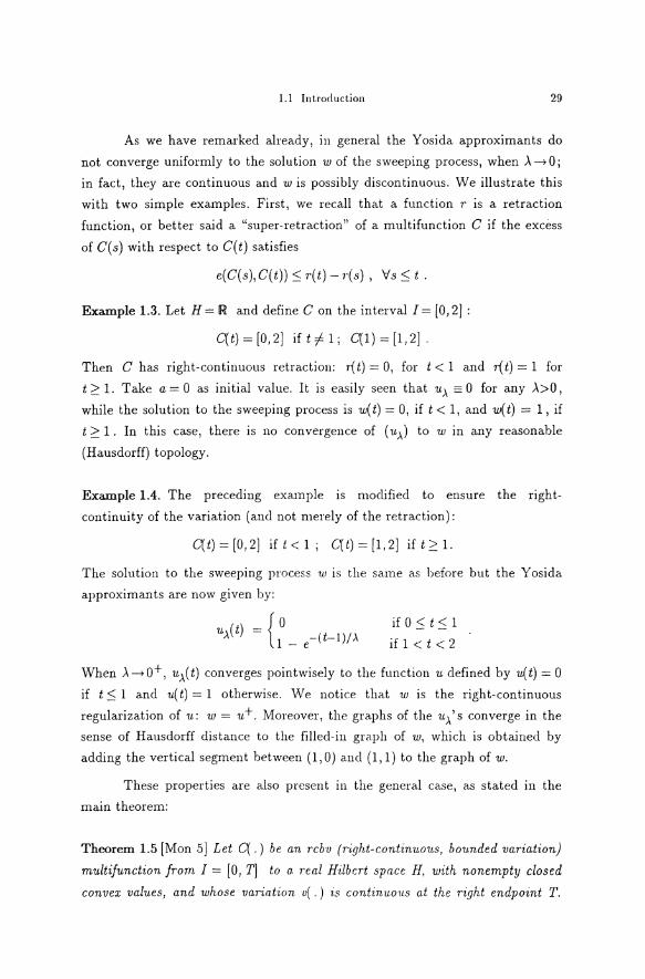
Example 1.4. The preceding example is moclified to ensure the right­

continuity of the variation (and not merely of the retraction):

C(t)=[0,2] ift<l; C(t)=[1,2] ift2:1.

The solution to the sweeping process w is the same as before but the Yosida

approximants are now given by:

e-(t-1)/.A if 0::::; t::::; 1

if 1 < t < 2

When .\-->0+, u).(t) converges pointwisely to the function u defined by u(t) = 0

if t::::; 1 and u( t) = 1 otherwise. We notice that w is the right-continuous

regularization of u: w = u+. Moreover, the graphs of the u).'s converge in the

sense of Hausdorff distance to the filled-in graph of w, which is obtained by

adding the vertical segment between ( 1, 0) ancl (1, 1) to the graph of w.

These properties are also presen t in the genera.l case, a.s stated in the

main theorem:

Theorem 1.5 [Mon 5] Let C(.) be an rcbu (right-contin·uous, bounded va.riation}

multifunction from I = [0, T] to a. 1·eal Hdbcrt spnce H, with nonempty closed

convex values, and whose varintion u( . ) is contin·uo·us a.t the right endpoint T.

30 Chapter 1: Regularization and Graph Approximation of a Discontinuous Evolution

Moreover, suppose that, denoting by B the open unit ba~l of H:

(8) C(t) n rB is strongly compact, for ever-y tc I and every r > 0.

Let aE: C(O) and consider the respective Yosida approximants uA (..X> 0).

a) When ..X-; 0, uA converges po·intwisely to w-, where w is the solution to

the sweeping process (2)-( 4) (see Definit·ion 1.1):

(9)

b) When .,X-;0, uA converges to w in the sense of filled-in graphs, that is:

(10) h(gr uA , gr* w) -; 0 ;

c) When .,X-;0, there is a strong convergence, ·uniformly on I:

(11) proj(uA(t), C(t))-; w(t) (tel).

The proof runs as follows. Since IR is metrizable, it suffices to assume that ..X takes a sequence of positive va.lues converging to zero. In section 2, we

give some estimates on the L1-uonn of the derivatives of the Yosida

approximants. This allows extraction of a subsequence which is weakly

pointwisely convergent to a bv function u, which turns out to be left­

continuous. In section 3, several properties of u and u+ are established; in

particular, strong pointwise convergence is derivecl from hypothesis (8). In

section 4, it is shown that u+ is the solution to the sweeping process and by

uniqueness the first part follows. In section 5, we study the graph convergence

of (uA) and prove (10) and (11) with a similar technique. Notice that theorem

0.3.4 on the extraction of convergent subsequences, in the sense of filled-in

graphs, does not apply here, tlms forcing some Ievel of complexity on the

proof.

1.2. Preliminary estimates duA We aim at obtaining an upper bound of the Hilbert norm of dt (t) using to

that effect some approximations of uA .

Let v : I-; IR be the variation function of C ( or more generally a

"super-variation", i. e., a function that satisfies (1.1 )) . By assumption, v has

bounded variation (since v is nondecreasing, this is equivalent to v( T) c IR), it is

1.2 Prelirninary estimates 31

right-continuous on I and continuous at T: v-( T) = v( T). Hence, for every

€ > 0, it is possible to find a partition Pf of the interval I:

io=O< t1 < ... < tm < T= tm+l

such that, putting I;= [t; 1 ti+l[ for 0 S:: i < m and Im = [tm 1 T], we have, for every i:

(1) length( I;) :::; € , osc( v,I;) :::; €.

To Pi we associate a step-multifunction Cf defined by

which satisfies, for every t:

(2) h( Cf(t) 1 C(t)) = h.( C(t;) 1 C(t)) S:: v(t)- v(t;) S:: € •

For technical reasons, we shall tempora.rily consider an arbitrary initial

value ae Hand denote by u,\, respectively by uf,,\, the absolutely continuous

solution of (1.6)-(1.7), respectively of

duE, ,\ 1 .. (3) ~ (t) + 'X [uE,,\(t)- proJ( 1Lf,,\(t), Cf(t))] 0, a. e. on I

wi th the ini tial condi tion uf ,\ ( 0) = a. '

From the elementary theory of orclina.ry differential equations follow

the equivalent integral formulations [Bre 1]:

(4) u,\(t) = e-tf,\ a + -!; jt e(s-t)f,\ proj(u,\(s) 1 C(s)) ds;

0

(5) u~;,,\(t) = e-tf,\ a + ± jt e(s-t)f,\ proj(uf,,\(s) 1 Cf(s)) ds.

0

The latter ca.n be computed explicitly. Let

b = proj( a, C(O)).

Since Cf( t) = C(O) for 0 S:: t < t1 , we guess that, for these values of t, uf, ,\( t) must belong to the segment [a1 b], i.e., ui,,\(t) = b + 1/;(t)(a-b), with

0:::; tjJ(t):::; 1 and t/J(O) = 1. This reduces equa.tion (3) to

dt/J 1 dt(t) (a-b) + 'X t/J(t)(a-b) = 0 a. e.,

smce proj( u" ,\( t) 1 C(O)) = b. Solving this Ca.uchy problern for t/J, m the nontrivial cas~ af. b, gives 1/;(t) = e-tf,\; so, for tei0 ,

uf ,\(t) = b + e-tf,\ (a-b). '

32 Chapter 1: Regularization and Graph Approxirna.t.ion of a Discontinuous Evolution

Proceeding in the sa.me ma.nuer wheu we consider the other

subintervals, it is easily checked tha.t, if xi = u,,,A(ti) = (u,,.A)- (ti) and

Yi = proj(xi, C(ti)) (in particula.r, x0 = a, y0 = b), then, for tc; Ii:

(6)

(7)

-(1-1·)/.A u,,,A(t) = Yi + e ' (x;-vj).

We want to show tha.t these functions uc, .A converge to u.A as E----t 0.

With this aim, we prove the following inequa.lity for tc: Ii:

II uc ,A(t)-proj(u, ,A(t), C,(t)) II :S e-I/.A II a-b II ' '

i -(1-1·)/.A + L e J (r(tj)-r(tj_ 1)),

j=1

where r(.) is a retraction function of C, or a. "super-retra.ction", meaning that:

e( C(s), C(t)) :S r(t)- r(s) (s::; t) .

Proof of (7). Since u,,.A is continuous, (6) implies

-(t +1-t )/.A II xj+l- Yj II = e J J II xj - Yj II ·

Moreover, if j ~ 1, then since Yj- 1 c C(tj-l) we have

and so

llxj-Yjll clist(xj,C(tj)) :S II xj-Yj- 1 11 + dist(Yj-l•C(tj))

-(lj-lj-1)/.A < e II xj-1- Yj-III + r(tj)-r(tj-l) ·

-1 /.A Therefore,forj=l, llx1-v1 11 :Se 1 lla-bll +r(t1)-r(la); forj=2,

II xrY2II :S e-(I2- 11 )/.A[ e-ll/.A II a-b II + r(tl)-r(la)] + r(t.2)-r(t1)

= e-12/)...11 a-b II + e-(12-11)/.A[r(tl)-r(la)] + e-(12-12)/.A[r(~)-r(t1)]'

and by induction

-1·/.A i -(1--1 ·)/.A llxi-Yill :Se' lla-bll + L e ' 1 [r(tj)-r(tj-1)].

j=1

This inequality implies (7) beca.use, if we consider tc: Ii, then by (6) we have:

-(1-1 )/.A II u,,..\(t)- proj(u,jt), C,(t)) II = ll·u,,.A(t)-y;ll = e 1 II xi-Yi II- D

Note that in (7):

1.2 Preliminary estimatcs 33

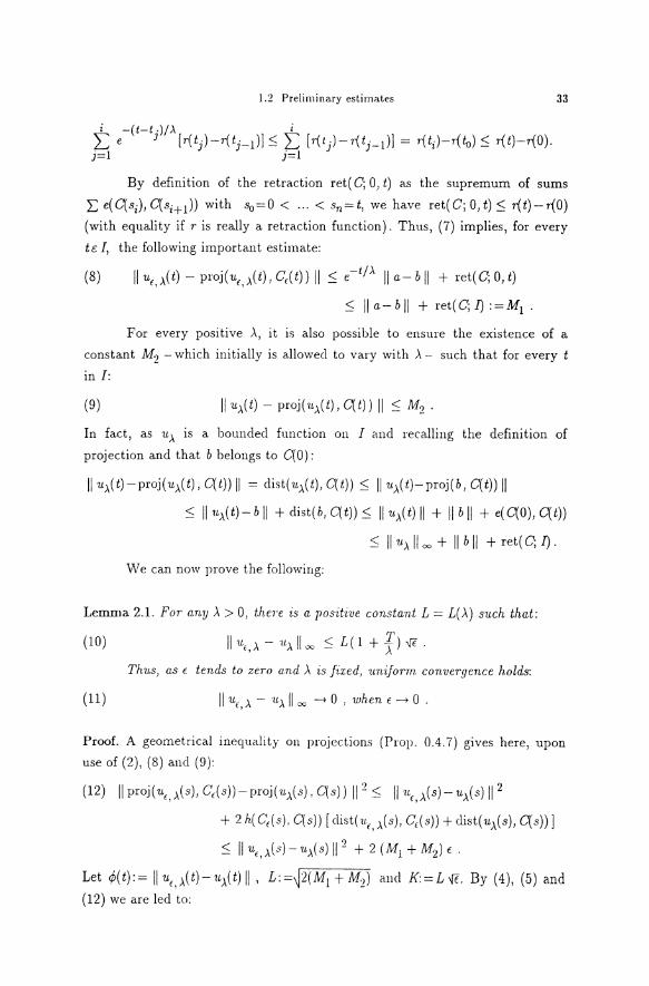
By definition of the retraction ret( C; 0, t) as the supremum of sums

I; e(C(si),C(si+l)) with s0 =0 < ... < sn=t, we have ret(C;O,t)~ r(t)-r(O) (with equality if r is really a retraction function). Thus, (7) implies, for every

tE: I, the following important estimate:

(8) llut.\(t)-proj(ut.\(t),C,(t))ll::::; e-tj>.lla-bll + ret(C;O,t) ' '

::::; II a-b II + ret(C; I) :=M1 .

For every positive ..\, it is also possible to ensure the existence of a

constant M2 - which initially is allowecl to vary with ,\- such that for every t

in I:

(9) II u>.(t)- proj(1t>.(t), C(t)) II ::::; M2 .

In fact, as u). 1s a bouncled function on I ancl recalling the definition of

projection and that b belongs to C(O):

II u>.(t)-proj(u>.(t), C(t)) II = dist(1t>.(t), C(t))::::; II u>.(t)-proj(b, C(t)) II ::::; 111t>.(t)- b II + c!ist(b, C(t))::::; II u>.(t) II + 11 b II + e(C(O), C(t))

::::; II u>.ll = + II b II + ret( C; I).

W e can now prove the following:

Lemma 2.1. For any ,\ > 0, ther·e is a positive constant L = L(A) such that:

(10) ll·u,,>.- ·u>.lloo ::=:; L(l +fJ fE ·

Thv.s, as c tends to zero and ,\ is fixed, 1mijorm convergence holds:

(11) II u, ). - u>.ll = ---> 0 , when f ---> 0 . ,

Proof. A geometrical inequality on projections (Prop. 0.4.7) gives here, upon

use of (2), (8) and (9 ):

(12) II proj(u,,>.(s), C,(s))-proj(u>.(s), C(s)) 11 2 ::::; lln,,>.(s)-n>.(s) 11 2

+ 2 h( C,(s), C(s)) [ clist{v,,>.(s), C,(s)) + clist(n>.(s), C(s))]

::=:; II u,,).(s)-1t).(s) 11 2 + 2 (M1 + M2) E.

Let rf;( t): = II u,, >.( t)- u>.(t) II , L: =~2( M1 + M2) ancl K: = L '{f.. By ( 4), (5) and (12) we are lecl to:

34 Chapter 1: Regularization and Graph Approximation of a Discontinuous Evolution

hence,

<P(t) :=:; ± jt e(s-t)f>. ~ </J(s)2 + L2f ds, 0

<fJ(t) :=:; L {E (1- e-tf>.) + jt ± e(s-t)f>.</J(s)ds :=:; K + 7/;(t),

0 where 7/;( t) derrotes the last integral. Since 7/;(0) = 0 and

d'lj; - 1 (A.. ·'·) < K I dl - "X 'f'- 'f' _ T a. e. on ,

it follows that

whence (10). 0

Denoting by dr the differential or Stieltjes measure of the retraction

function r, we state:

Theorem 2. 2. For every m I and every positive >., the following estimate

holds:

(13) :=;e-tf>.iia-bll + 1 e(s-t)f>.dr(s) [0, t]

:=:; iia-bll +ret(C;O,t).

Proof. When f ---7 0, C{( t) converges to C( t) in the sense of Hausdorff distance,

as is clear from (2), whereas by (11 ), uf, >.( t) converges strongly in H to u>.( t).

Hence the left-hand side of inequality (7) converges to the left-hand side of (13)

(see (12) or use the continuity of the projection into a fixed convex set). We

further remark that the sum appea.ring in the right-hand siele of (7) is bounded

above by

t e(tj-t)j>.[r(tj)-1'(tj-l)] + p-t)f>. [r(t)-r(tj)]. j==l

This is a Stieltjes sum for the integra.l over [0, t] of the continuous function s---7 e(s-t)/).. with respect to the differential measure dr. Since by construction

the subdivision Pf = { l:o, ... , tm+l} satisfies (1), we have dr(int Ii) = osc( r, Ii) :=:; osc( v, Ii) :=:; f and these Stieltjes sums converge to the sa.id integral when f

tends to zero. So, inequality (7) implies the first inequa.lity in (13).

The second inequality in (13) is now immediate, because

1 e(s-t)f>. dr(s) :=:; 1 dr\s) = r{t)-r(O). (0, t] (0, t]

0

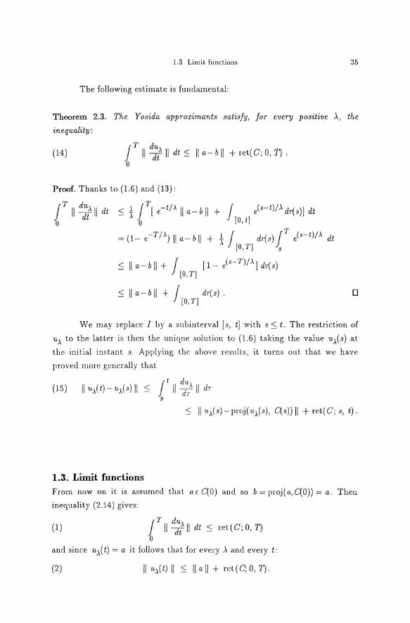
1.3 Limit functions 35

The following estimate is fundamental:

Theorem 2.3. The Yosida approximants satisfy, for every positive )., the

inequality:

(14) JT II d~~>. II dt:::; II a-b II + ret(C; 0, T). 0

Proof. Thanks to (1.6) and (13):

jr II d:t II dt 0

:::; ± jT[ e-t/>. II a-b II + j e(s-t)/>. dr(s)] dt 0 [0' t]

= (1- e-Tj>.) II a-b II + ± j dr(s) JT e(s-t)J>. dt [O,T] s

:::; lla-bll+ j [1-e(s-T)j>.]dr(s) [O,T]

:::; II a-b II + j dr(s). [O,T]

0

We may replace I by a subinterval [s, t] with s:::; t. The restriction of

u>. to the latter is then the unique solution to (1.6) taking the value u>.(s) at

the initial instaut s. Applying thc a.bove results, it turns out that we have

proved more gencrally that

(15) II u>.(t)-11>.(s) II :::; j 1 II d~~;., II dr s

:::; ll11>.(s)-proj(u>.(s), C(s)) II + ret(C; s, t).

1.3. Limit functions From now on it is assumed that ac C(O) and so b = proj(a,C(O)) = a. Then

inequa.lity (2.14) gives:

(1) JT du II d/ II dt :::; ret ( C; 0, T)

0

and since u >. ( t) = a i t follows that for eveq ). ancl every t:

(2) ll1t>.(t) II :::; II a II + ret(C; 0, T).

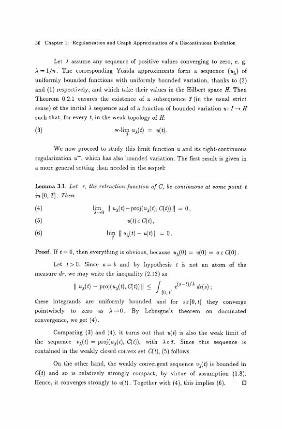
36 Chapter 1: Regularization and Graph Approximation of a Discontinuous Evolution

Let ). assume any sequence of positive values converging to zero, e. g.

). = 1/n. The corresponding Yosida approximants form a sequence (uA) of

uniformly bounded functions with uniformly bounded variation, thanks to (2) and (1) respectively, and which take their values in the Hilbert space H. Then Theorem 0.2.1 ensures the existence of a subsequence :f (in the usual strict

sense) of the initial ). sequence and of a function of bounded variation u: I---+ H such that, for every t, in the weak topology of H:

{3) w-lim uA( t) = u( t). ':1

We now proceed to study this Iimit function u and its right-continuous

regularization u+, which has also bouncled variation. The first result is given in

a more general setting than neecled in the sequel:

Lemma 3.1. Let r, the retraction function of C, be continuous at some point t in [0, J1. Then:

(4)

(5)

(6)

l{~o /1 uA( t)- proj( uA( t), C( t)) II == 0,

u(t).o C(t),

!im II uA(t)- u(t) II == o. 'i

Proof. lf t == 0, then everything is obvious, because uA(O) == u(O) == a c C(O).

Let t > 0. Since a == b and by hypothesis t is not an atom of the

measure dr, we may write the inequality (2.13) as

II uA(t)- proj(uA(t), C(t)) II :::; j e(s-t)j>. dr(s); [0, t[

these integrands are uniformly bounded and for sc [0, t[ they converge

pointwisely to zero as .>.---+ 0. By Lebesgue's theorem on dominated

convergence, we get (4).

Comparing (3) and (4), it turns out that u(t) is also the weak Iimit of

the sequence vA( t) == proj( uA( t), C( t)), with ). c :f. Since this sequence is

contained in the weakly closed convex set C(t), (5) follows.

On the other hand, the weakly convergent sequence vA(t) is bounded in

C( t) and so is relatively strongly compact, by virtue of assumption (1.8).

Hence, it converges strongly to u(t). Tagether with (4), this implies (6). 0

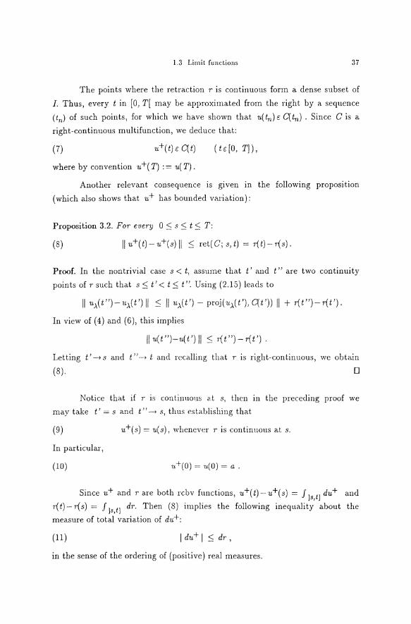
1.3 Limit. functions 37

The points where the retraction r is continuous form a dense subset of

I. Thus, every t in [0, T[ may be approximatecl from the right by a sequence

(tn) of such points, for which we have shown that u( tn) E C( tn) . Since Cis a

right-continuous multifunction, we decluce that:

(7) (tc:[O, T]),

where by convention u+( T) : = u( T).

Another relevant consequence 1s given m the following proposition

(which also shows that u+ has bounclecl varia.tion):

Proposition 3.2. For e-very 0 :=::; s :=::; t :=::; T:

(8) II u+(t)-·u+(s) II :=::; ret(C; s, t) = r{t)-r{s).

Proof. In the nontrivial ca.se s < t, asslune that t' ancl t" are two continuity

points of r suchthat s :=::; t' < t :=::; t". Using (2.15) leacls to

II u,\(t")- u,\(t') II :=::; 111t;,(t')- proj(u;,(t'), C(t')) II + r{t")- r{t').

In view of (4) ancl (6), this implies

II u(t")-u(t') 11 :=::; 1'(t")- r{t').

Letting t' --t s ancl t "--t t a.ncl reca.lling that r is right-continuous, wc obtain

(8). D

Notice that if r is continuous at s, then in the preceding proof we

rnay take t' = s and t "--t s, tlms establishing that

(9) u+(s) = u(s), whenever r is continuous at s.

In particular,

(10)

Since u+ a.nd r a.re both rcbv functions, u+(t)- u+( s) = J ]s,t] du+ and

r{t)-r{s) = f]s,t] dr. Then (8) implies the following inequality about the

rneasure of total va.riation of du+:

(11) I du+ I :=::; dr,

in the sense of the orclering of (positive) real measures.

38 Chapter 1: Regularization and Graph Approximation of a Discontinuous Evolution

Proposition 3.3. The pointwise Iimit function u is left-continuous:

(12)

and strong convergence holds:

(13) lim II u..\(t)-u(t) II = 0 'j

(tel)

(te I) .

Proof. In view of (3) and by uniqueness of Iimits we only need to prove that:

(14) (td).

If t = 0, (12) holds by convention and (14) is obvious. If te )0, T), given an

arbitrary € > 0 we choose s < t such that r is continuous at s and

r-(t)-r(s)5€. By Lemma 3.1, for sufficiently smal(>. in the subsequence 1

the following inequalities hold simulta.neously:

Then, for any t'in [s,4, recalling (2.15):

II u..\(t')-u..\(s) II 5 € + r(t')-r(s) 5 f.+r-(t)-r(s) 5 2€.

Together with (8) and (9) this now gives:

(15) II u..\(t~-u+(t~ II 5 II u..\(t~-u..\(s) II + II u..\(s)-u(s) II + II u+(s)-u+(t~ II 5 3€+r(t~-r(s) 5 4€.

Fixing>. in the afore-mentioned conditions, we take Iimits as t'--+ t, obtaining:

because u..\ is continuous a.nd (u+)- = u- . Hence (14) holds. D

From (8) and (12) we readily infer that:

(16)

We end this section with a statement which is more precise than (7):

Proposition 3.4. For every t in I, we have

(17) u+(t) = proj(u(t), C(t)) .

Proof. If t = T, this is clear by (7) and the convention thereafter. If t < T, Iet

t'> t. By (2.15), II u..\(t~- u..\(t) II 5 dist(u..\(t), C(t))+ret(C; t, t1.

Taking Iimits with respect to the subsequence j and profiting from (13) and

1.4 The solution 39

from the strong continuity of the distance to a fixed set, we get:

II u(t')-u(t) II ~ c!ist(1t(t), C(t))+r(t')-r(t).

Letting t' converge to t and remembering that r is right-continuous, this

implies that

II u+(t)-u(t) II ~ dist(u(t), C(t)).

Since u+( t) c C( t) (by (7) ), this characterizes u+( t) as the projection of u( t). D

1.4. The solution We shall prove that w: = u + is thc solution to the sweeping process (1.2)-(1.3)

urith initial value a.

We know that w has bounded variation (3.8) a.nd is of course right­

continuous. In view of (3.10), it satisfies the prescribed initial conclition and

(3.7) - or (3.17) - means that w(t)c- C(t) for every t in I. Hence all we have

to show is (1.4), that is, choosing dJt= I du+ I:

(1)

for I du+ I -almost every t in I. Notice that the measures du and du+ are equal

on I and have no atoms at the endpoii1ts t = 0 and t = T, because of (3.10)

and since u-(T) = u(T), by (3.12).

If tc-]0, T[ is an atom of du+= d11,, we have by (3.12) a.nd (3.17):

_ dn+_ (t) = __ ·u+(t)-·u-(t) u(t)-proj(u.(t),C(t)) !du+! llu+(t)-1L-(t)ll - llu(t)-proj(u(t),C(t))ll ·

By the property of projections, this vector belongs to the outward normal cone

to the convex set C(t) at the point 1t+(t) = proj(u(t), C(t)). So, we have

established that ( 1) holds at every atom.

Next, we shall consicler the points at which 11+ (and hence u) is

continuous. Tobe precise, because (1) is tobe verified only du+-a.]most

everywhere, we only neecl to consider the points t where the retraction r is

continuous. This exclucles a countable set, possibly formecl by: 1) the atoms of

du= du+, already stucliecl, ancl 2) a subset of continnity points for u+ (hence

du+-null points) which is then d·u+-null itself.

40 Chapter 1: Regularization and Graph Approximation of a Discontinuous Evolution

The following lemma is usecl to obtain ( 1 ).

Lemma 4.1. If an rcbv function </>: [t, tj ~ H zs a selection of C (i.e.,

<f>(s) t: C(s) for every s in the interva~ then:

(2) J </> · du ?. ~ ( Jl u( t ') 11 2 - II u( t) 11 2 ) · (t, t'( -

Proof. Recall that here J [t,t '[ </>.du:= J [t,t '[ (</>. I~: I ) I du I t: IR, where the

density I~~ I belongs to 1.1(!, I du I; H) .

We still use the notation vA(s) = proj(uA(s), C(s)). By definition (1.6), the

Yosida approximants satisfy, for (Lebesgue) almost every s: du, d:i"(s) = ! (vA(s)-uA(s)).

Since <f>(s)t: C(s) ancl ,\ is positive, this implies by a well-known property of

projections:

Then

and since

du [<f>(s)-vA(s)]. dsA(s)?. 0, a.e. in [ t, t '].

duA duA dnA 1 duA vA. ds = (vA-uA). ds +"!LA. ds = (-uA-uA). [x(vA-uA)]+ uA "ds

it follows that

and

J t' j t' d·uA 2 ? </J.duA ?_ uA.dsds= 1(11uA(t')JI -JiuA(t)JI-).

t t

We take Iimits with respect to >.. Since the continuous functions uA converge

pointwisely weakly to the left-continuous function u and since </> is right­

continuous with bounded variation, we may apply Theorem 0.2.l.(ii) to

the left-hand siele of the last inequa.lity, obta.ining:

t' j </>. duA = j </>. duA ~ j </>. du . t [ t, t'( [t, t '[

Recalling (3.13) yields the desired property. 0

1.4 The solution 41

Let t be a continuity point of the retraction r.

By (3.8), u+ is also continuous at t. For every x in the convex set C( t) we pick an rcbv selection of C defined in [ t, T], say </>, such that </>( t) = x. This

can be clone, for instance, by considering the sweeping process with this initial

condition and applying the results obtained so far. Notice that the "obvious"

choice s--+ proj(x, C(s)) rnay have unbounded variation. By (2), if f > 0 is

sufficiently srnall, we have

J </>.du ;::: !( II u( t+c) 11 2 -II u(t) 11 2 ) = ~[u(t+c) + u( t)]. [u(t+c)-u(t)]. [t, t+([ -

We write </> = x-(x-<1>) and choose f in such a way that u is also

continuous at t+E, so that du([ t, t+c[) = ·u( t+E )-u( t) = du([ t, t+E]). We get

x. du([ t, t+c]) ;::: ~[ u( t+c) + u( t)]. du([ t,t+c]) + j ( x- </>).du, - [t, t+(]

whence

( x - ! [ u( t+E) + u( t)] ) . du([ t, t+E]) ;::: - osc( </>, [ t, t + f]) I du I ([ t, t + f]) .

Divide by I du I ([t, t+c]) (with the convention 0/0 = 0) and let c--+0, picking

only continuity points t+c. By virtue of Jeffery's theorern on the densities of

rneasures (Theorem 0.1.1), this gives:

lirp (x-![u(t+t)+u(t)]). ~~~~(t) ;:::-lirposc(,P,[t, t+c]),

for I du I -alrnost every t satisfying the above conditions. So, because u 1s

continuous at t and </> is right-continuous:

(x-1t(t)). I ~~I (t) ;::: o, for every x in C( t). This is equivalent to

- I~:~ I (t)c NC(t)(u(t)),

which expresses precisely the sarne as (1), since t is a continuity point.

In short, we have shown so far that, if .A takes any sequence of positive

values converging to zero and if 1 is any subsequence ensuring the pointwise

weak convergence of the Yosicla approxirnants (u,\) with .Ac1, then these

approxirnants converge pointwisely strongly to ·u = w- (see (3.13)) where

w = u+ is the unique solution to the sweeping process. A standard reasoning

shows that, for every t and every xc H, w-( t). x is the unique sublirnit and

hence the lirnit of the relatively compact sequence of real nurnbers ( u,\( t). x).

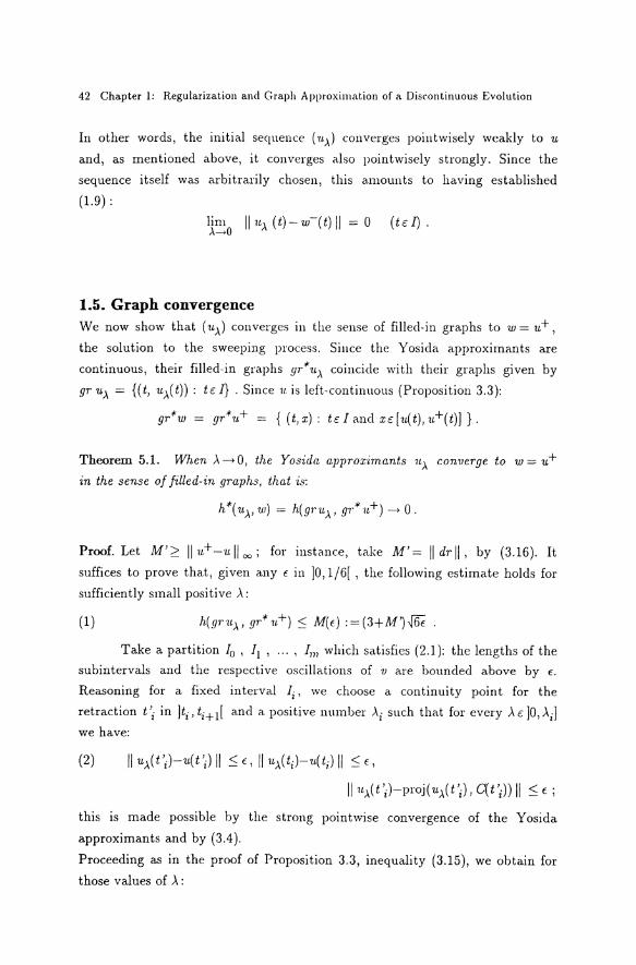
42 Chapter 1: Regularization and Graph Approximation of a Discontinuous Evolution

In other words, the initial sequence (u-') converges pointwisely weakly to u

and, as mentioned above, it converges also pointwisely strongly. Since the

sequence itself was arbitrarily chosen, this amounts to having established

(1.9):

1.5. Graph convergence We now show that (1t-') converges in the sense of filled-in graphs to w = u+,

the solution to the sweeping process. Siuce the Y osicla approximants are

continuous, their filled-in graphs gr*1t-' coincide with their graphs given by

gr u-' = {(t, u-'(t)): tc I} . Since 1t is left-continuous (Proposition 3.3):

gr*w = gr*·u+ = { ( t, x) : tc! and Xe [ u( t), u+( t)] } .

Theorem 5.1. When >.--> 0, the Yos-ida a.pprox-im.ants u-' converge to w = u+

in the sense of Jilled-in graphs, that is:

h*(u-',w) = h(g7"u-', gr*·u+)--> 0.

Proof. Let M'?_ ll·u+-ulloo; for iustance, take M'= lldrll, by (3.16). It

suffices to prove that, given any E in ]0, 1/6[ , the following estimate holds for

sufficiently small positive ). :

(1)

Take a partition I0 , I 1 , ... , I 171 which satisfies (2.1): the lengths of the

subintervals and the respective oscillations of ·v are bounded above by E.

Reasoning for a fixed interval I;, we choose a continuity point for the

retraction t '; in ]t;, ti+l[ and a positive number \ such that for every ). c ]0, >.;] we have:

(2) llu-'(t';)-u(t';)ll ~E, llu-'(t;)-u(t;)ll ~E,

111t-'(t';)-proj(u-'(t';), C(t'i)) II ~ E;

this is made possible by the strong pointwise convergence of the Yosida

approximants and by (3.4).

Proceeding as in the proof of Proposition 3.3, inequality (3.15), we obtain for

those values of ). :

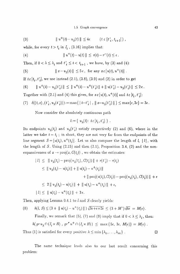
1.5 Graph convergence 43

(3)

while, for every t > ti in Ii , (3.16) implies that:

(4)

Then, if 0 < ,\ :S ,\i and t'i :S t < ti+l , we have, by (3) and (4):

(5) llx-u,x(t)ll :S5E, foranyxc[u(t),u+(t)].

If tc:[ti,t';], we use instead (2.1), (3.8), (3.9) ancl (2) in order to get

(6) 11 u+(t)- u_x(t'J II ::::; II u+(t)- u+(t';) 11 + 11 u(t'j)- u_x(t'j) 11 ::::; 2€.

Together with (2.1) and (4) this gives, for xc:[u(t), u+(t)] and tc: ]ti, t'J (7) 6((t,x),(t';,u,x(t';))):=max{lt-t';l, llx-u,x(t'i)II}:Smax{E,3E}=3E.

N ow consider the absolutely continuous path

Its endpoints u,x( t;) and u,x( t ';) satisfy respectively (2) and (6), where in the

latter we take t = t; ; in short, they are not very far from the endpoints of the

line segment S = [u( t;), u+(t;)]. Let us also compare the length of l, lll, with

the length of S. Using (2.15) and then (2.1 ), Proposition 3.4, (2) and the non­

expansiveness of x-> proj(x, C(t;)) , we obtain the estimates:

111 ::::; 11 u_x(t;) -proj(11_x(t;), C(t;ll 11 + r(t';)- r(t;)

::::; lln,x(t;l- 1t( t;) II +I Iu( t;)- 11+( t;) II

+ II proj( u( t;), C( t;))- proj( u,x( t;), C( t;)) II + E

< 2lln_x( t;)- 11( t;) II + II u( t;)- n+(t;) II + €,

lll ::::; lln( t;)- 1t+(t;) II + 3 €.

Then, applying Lemma 0.4.1 to I and S clearly yielcls:

Finally, we remark that (5 ), (7) ancl (8) imply that if 0 < ,\ :S \, then:

h(grn,xn(I;xHJ, gr*v+n(I;xfi))::::; max{5E, 3E, M(c)} = M(c).

Th us ( 1) is satisfied for every positive ,\ :S min {,\0 , ... , Am} . 0

The samc techniquc Ieads also to our last result concerning this

problem:

44 Chapter 1: Regularization and Graph Approximation of a Discontinuous Evolution

Theorem 5.2. The projections of the Yosida approximants, denoted by

v_x(t):=proj(u,x(t), C(t)), converge uniformly in the norm of H to the solution to

the sweeping process w = u+, as A-->0.

Proof. Let 0 < € < ~ be given and choose any partition ( Ii) of the interval I satisfying (2.1). We have seen that (3) and (8) hold for every i and every

sufficiently small .\. We consider two cases separately.

If tc[t'i, ti+l[, then by (3.7) ancl (3):

(9) II v_x(t)- u+(t) II II proj(u_x(t), C(t))- proj(u+(t), C(t)) II

< lju._x(t) -1L+(t) II :S 4€.

Let now tc[ti, t'i]. In view of (8), u,x(t) is not far from the line segment

S; to be precise, there exists xc: [ u( ti), u +( ti)] such that

II u_x( t)- x 11 2 :::; 6(3 + M')2 E.

But u+(ti), which by (3.17) is the projection of u( ti) in C( t;), is clearly also the

projection of x. Hence, by application of (2.2), (2.13), (3.8) and of the

inequality on projections (Prop. 0.4. 7):

II v_x(t)- u+(t) II :S II proj(u_x(t), C(t))- proj(x, C(t;)) II + II u+(t;)- u+(t) II

:S~IIu_x(t)-xll 2 +2h(C(t),C(t;))[liu_x(t)-v_x(t)li + llx-u+(t;)IIJ + €

:S ~6(3 + M')2 f + 2 € [ II dr II + M'] + € .

This is an upper bouncl which is inclepenclent of >. ancl which converges to zero

asE-+0.

From this ancl (9) the result is reaclily obtainecl. D

Chapter2

Sweeping Processes by Convex Sets with N onempty Interior

2.1. Introduction In this Chapter, weshall deal with the sweeping process (Definition 1.1.1) by a

moving convex set t--t C(t) with nonempty interior. Sometimes the convex set

C( t) may be decomposed in the form

C(t) = v(t) + r(t),

where V is a function taking values in a separable Hilbert space H and r is a

multifunction with closed convex values having nonempty interior in H. If v is

continuous and r is Lipschitz-continuous in the sense of Hausdorff distance,

then the first proof of existence of a solution is due to Castaing ([Cas 1] Th. 6).

It generalizes a previous statement by Tanaka [Tan], where r is constant and

H is finite-dimensional. Since C need not have a bounded retraction, the

assumption on the interior of the convex set is essential. For instance, if we

take r( t) = {0}, then only the function v coulcl be a solution to the sweeping

process, but v may have unbounded Variation.

More generally, we establish here the existence of a solution m the

following two cases:

a) C( t) is Hausdorff-continuous ancl H JS a Hilbert space of arbitrary

dimension (sections 2 and 3 );

b) C(t) is lower semicontinuous (from the right) and H JS finite-

dimensional (section 4).

Uniqueness follows from the monotonicity of the outward normal cone;

see [Mor 1, 5] and [Mor 6] (Prop. (6.b)). A random or parametric version of the sweeping process is also studied (Theorem 3.8).

In the implicit kynematical interpretation of this mathematical

problem, the fundamental result achievecl is that, in both the above cases, the driven ( swept) system has a bounded variation motion even if the driving

(sweeping) system has not.

Proofs are based on the catching-up algorithm conveniently adapted to

this new type of assumption.

46 Chapter 2: Sweeping Processes by Convex Sets with Nonempty Interior

2.2. Continuous convex set in arbitrary dimension: preliminary results

Consider I= [0, T], a real Hilbert space H with arbitrary dimension and a

multifunction t--> C( t) defined on I whose values are closed convex subsets of

H with nonempty interior. It is assumed that Cis Hausdorff-continuous, i. e.,

continuous in the sense of the Hausdorff distance h relative to the metric

associated with the Hilbert norm of H. This means that, for any s in I:

(1) h( C(t), C(s))--> 0, as t--> s.

Note that this condition does not require that the convex sets be bounded, but

clearly implies that h( C( t), C( s)) be finite for every s and t.

We prove that the sweeping process by such a moving convex set C has

a solution.

Theorem 2.1. Under the given hypotheses, for every initial value ~ c C(O) there

is one and only one cbv ( continuous with bounded variation) function u: I--> H

such that:

(2)

(3)

(4)

u(O) = ~;

u( t) c C( t) ( t c I) ;

- i ~~~ (t) c NC(t) (u(t)), I dul-a. e ..

Note that the solution to the sweepmg process by C(t) is also the

solution to the sweeping process by C(t) n B(O, R), where R > II u II 00 (see the

proof of Lemma 4.2.2). Hence, if some a priori estimate is available, then we

may replace the initial multifunction by a bounded one, choosing an

appropriate R. This means that assumption ( 1) may be replaced by the

weaker:

(5) t--'>s=? h(C(t)nB(O,R),C(s)nB(O,R))-->0,

for every positive R.

In the general formulation of sweeping problems, it is only required that

the bv solution be right-continuous. The above theorem ensures that the

solution is continuous if the moving convex set is Hausdorff-continuous. That

this is true can be shown immediately:

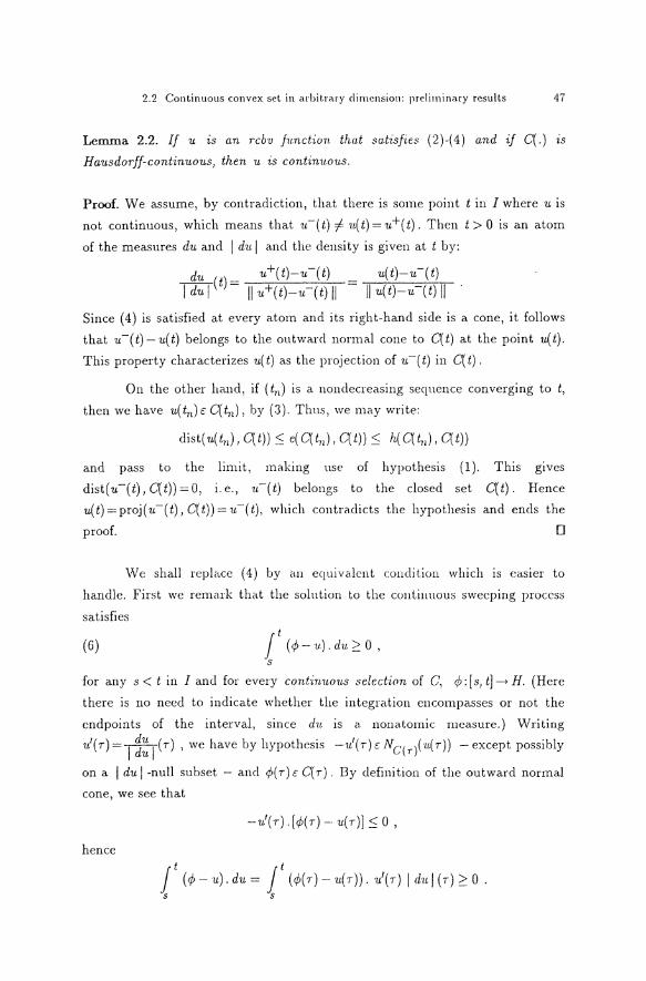
2.2 Continuous convex set in arbitrary dirncnsion: preliminary rcsults 47

Le=a 2.2. If u is an rcbv function that sa.tisfies (2)-(4) and if C(.) ts

Hausdorff-continuous, then u is contimw·us.

Proof. vVe assume, by contracliction, that there is some point t in I where u is

not continuous, which means that 1t-( t) oJ 11.( t) = u+( t). Then t > 0 is an atom

of the measures du ancl I d1t I ancl the clensity is given at t by:

Since (4) is satisfied at every atom and its right-hancl siele is a cone, it follows

that u-(t)-u(t) belongs to the outward normal cone to C(t) at the point u(t).

This property characterizes u( t) as the projection of u-( t) in C( t).

On the other hancl, if ( t11 ) is a nonclecrea.sing sequence converging to t,

then we have u(t71 )c: C(t11 ), by (3). Thus, we may write:

clist(u(t11), C(t))::; e(C(t11 ), C(t))::; h(C(t11 ), C(t))

and pass to the Iimit, maling use of hypothesis (1). This g1ves

dist(u-(t),C(t))=O, i.e., 1t-(t) belongs to the closecl set C(t). Hence

u(t)=proj(u-(t), C(t))=u-(t), which contra.dicts the hypothesis and encls the

proof. D

We shall replace (4) by au equivalcnt condition which is cas1er to

handle. First we remark that the solution to the contiuuous sweeping process

satisfies

(6) j 1 (<P-u.). du?. 0 , s

for any s < t in I and for every cont-irwons selection of C, <P: [ s, t]-> H. (Here

there is no neecl to indicate whether the integration encompasses or not the

cnclpoints of the interval, since du is a nonatomic measure.) Writing

u1(r)= I~~ I (r), we have by hypothesis -u'(r)c: NC(r{u(r)) - except possibly

on a I du I -null subset - a.ncl cp( T) E C( T). By definition of the outward normal

cone, we see that

hence

j t ( cp - ·u) . du = j t ( q\( T) - n( T)) . u1 ( T) I d1t I ( T) ?. 0 . s s

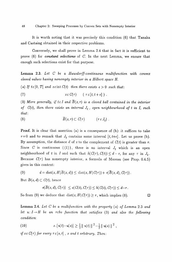
48 Chapter 2: Sweeping Processes by Convex Sets with Nonempty Interior

It is worth noting that it was precisely this condition (6) that Tanaka

and Castaing obtained in their respective problems.

Conversely, we shall prove in Lemma 2.4 that in fact it is sufficient to prove (6) for constant selections of C. In the next Lemma, we ensure that

enough such selections exist for that purpose.

Lemma 2.3. Let C be a Hausdorff-continuous multifunction with convex

closed values having nonempty interior in a Hilbert space H.

(a) IJ tc[O, T[ and zeint C(t) then there exists t: > 0 such that:

(7) zc C(r) ( TC [ t, t + t: j ) .

(b) More generally, if tt: I and B(z, r) is a closed ball contained in the interior

of C( t), then there exists an interval Jt , open neighbourhood of t in I, such

that:

(8) B(z, r) C C( r)

Proof. It is clear that assertion ( a) is a consequence of (b ): i t suffices to take

r= 0 and to remark that Jt contains some interval [ t, t+t:]. Let us prove (b ). By assumption, the dista.nce d of z to the complement of C( t) is greater than r.

Since C is continuous ( (1)), there is an interval Jt which is an open

neighbourhood oft in I and suchthat h(C(r), C(t)) ::=; d- r, for any Tin Jt· Because C(r) has nonempty interior, a formula of Moreau (see Prop. 0.4.5)

gives in this context:

(9) d = dist(z, H\B(z, d)) ::=; dist(z, H\ C(r)) + e(B(z, d), C(r)).

But B(z, d) C C( t), hence

e(B(z, d), C(r)) ::=; e(C(t), C(r)) ::=; h(C(t), C(r)) ::=; d-r.

So from (9) we deduce that dist( z, H\ C't T)) ~ r, which implies (8). D

Lemma 2.4. Let C be a multifnnction with the property ( a) of Lemma 2.3 and

let u: I-+ H be an rcbv function tha.t satisfies (3) and also the following

condition:

(10)

if zc C( T) for every TC [ s, t] , s and t n.rbitrary. Then:

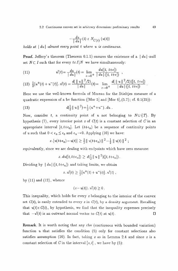
2.2 Continuous convex set in arbitrary dimcnsion: preliminary results 49

-I~~ I (t) c: NC(t) (u.(t))

holds at I du / -almost euery point t where u is continuous.

Proof. Jeffery's theorem (Theorem 0.1.1) ensures the existence of a /du /-null

set Ne !such that for every tc:I\N we have simultaneously:

(11) u1(t)= _ifu_(t) = lim du([t, t+c]) I du I ,_,0+ I du I ([ t, t+c]) '

? 2 l[u+(t)+u-(t)].u1(t)=d(llull-;2)(t)= lim d(llu/1 ;2)([t,t+c]) 2 /du/ <-->O+ /du/([t,t+c])

(12)

Here we use the well-known formula of Moreau for the Stieltjes measure of a

quadratic expression of a bv function ([Mor 5] and [Mor 6],(5.7); cf. 0.1(35)):

(13)

Now, consider t, a continuity point of u not belonging to NU { T}. By

hypothesis (7), every interior point z of C( t) is a constant selection of C in an

appropriate interval [ t, t+c0]. Let ( t+cn) be a sequence of continuity points

of u such that 0 < En::::; E0 and € 11 --+ 0. Applying (10) we have:

z. [ u( t+En)- u( t)] ~ ~ II ·u.( t+cn) 11 2 -! 1/ u( t) 1/ 2 ;

cquivalently, since we are dealing with endpoints which have zero measure:

l I 2 z. du([ t, t+c" ) ~ d(2// u II )([ t, t+cn]).

Dividing by / du/ ([ t, t+cnlJ ancl taking Iimits, we obtain

z. u1( t) ~ Hn+( t) + u-(t)].1t1( t) ,

by (11) and (12), whence

(z- u(t)). ·u-'(t) ~ 0.

This inequality, which holds for every z belonging to the interior of the convex

set C( t), is easily extended to every z in C( t), by a density argument. Recalling

that u( t) c: C( t), by hypothesis, we find that the inequality expresses precisely

that -u1( t) is an outward normal vector to C( t) at u( t). 0

R.emark. It is worth noting that any cbv (continuous with bounclecl variation)

function u that satisfies the condition (5) only for constant selections also

satisfies assumption (10). In fact, taking z as in Lemma 2.4 and since z is a

constant selection of Gin the interval [s, t], we have by (5):

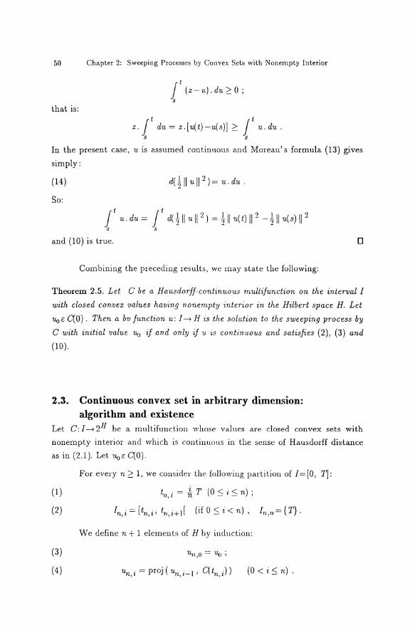
50 Chapter 2: Sweeping Processes by Convex Sets with Nonempty Interior

jt (z-u.).du~O; s

that is:

z. jt du= z.[u(t)-u(s)] ~ jt u.du. s s

In the present case, u is assumed continuous and Moreau' s formula (13) gives

simply:

(14)

So:

Jt Jt J I ? I ? u. du = d(! II u II ~ l = 2ll u( t) II - - 2ll u( s l II -

s s

and (10) is true. 0

Combining the preceding results, we may state the following:

Theorem 2.5. Let C be a Ha.1tsdorff-continuo'!Ls m1tltij1tnction on the interval I

with closed convex val'lLes having nonem.pty ·interior in the Hilbert space H. Let

Uot:C(O). Then a bvfnnction 'lL: !->His the soZ.ution to the sweeping process by

C with initial value 111l if a.nd only ·if ·u ·is contintwv.s and sa.tisfies (2), (3) and

(10).

2.3. Continuous convex set in arbitrary dimension: algorithm and existence

Let C: I---> 2H be a multifunction whose valnes are closed convex sets with

nonempty interior ancl which is continuous in the sense of Hausdorff distance

as in (2.1). Let 1J.ot:C(O).

(1)

(2)

(3)

(4)

For every n ~ 1, we consider the following partition of 1=[0, T]:

t · = .l T (0 < ·i < n) · n,z n - - '

In i = [ tn i , tn i + 1 [ ( i f 0 S i < n) , !11 , 71 = { T} . , ' '

We define n + 1 elements of H by induction:

11·n,o = 'Uo ;

(0 < i Sn) .

2.3 Continuous convex set in arbitrary dimension: algorithm and existence 51

These u 1• are used to define a right-continuous step-function u11 , n,

which is an approximant of the sohttion we are looking for:

(5) u11(t) = U 11 ,; , if tc 111 ,; (0:::; i:::; n) .

We also define a continuous piecewise affine approxima.nt v11 , given by:

t- tn i v (t) - u · + ' ( u · 1 - ·u ·) n - n, z t . 1 _ t . n, z+ n, z

n,t+ n,z (6) iftcl11 ,i (O:=;i<n)

and of course v11(T)=Un 71 , by continuity. I

We prove the following existence a.nd approxima.tion theorem:

Theorem 3.1. Both ( u11 ) and ( v11 ) conver·ge unijoTmly to u 1 the unique solution

to the sweeping pTocess (2.2)- (2.4).

First, we verify that ( 1t71 ) a.nd ('v71 ) do ha.ve the same uniform limit, if it

exists. In fact, v11( T) = u11 ( T) a.nd for t /= T it is clear that:

t- t . llvn(t)-un(t)ll=llt. :'~ _(un,i+!-un,JII:::; llun,i+l-un,ill

n1 ·t+l n,z

and I tn i - tn i+ I I ' '

(7)

where we put

=dist(1L11 ,; 1 C(tn,i+l)):::; h( C(t11 ,;), C(tn,i+l))

Tjn. Hence

II Vn- 1Ln II = :::; l 1n ,

(8) p 71 := sup { h( C(s), C(t)): t1 sei, I t- s I :::; Tjn} .

Notice tha.t (p11 ) is a nonincrea.sing sequence tha.t converges to zero:

(9) 0,

thanks to assumption (2.1) ancl to a. cla.ssica.l a.rgument invoking the

compa.ctness of the interva.l I. Combining (9) with (7) we get the expected

result.

The next step is to obtain estima.tes for the functions u11 and their

variations ( and which also hold for the continuous approximants v11):

Lemma 3.2. (a) There exist posit-i·ve constants L and M such that1 for every n:

(10) II un( t) II :::; L ( tc: I) ;

52 Chapter 2: Sweeping Processes by Convex s~t.s with Nonempty Interior

(11) var(u,,; I) :::; M.

(b) More precisely, if all the con-uex sets C( t) contain the ball B( a, r),

we may take

(12) L = II ·u'O II + II ·llv- a II ,

(13) M= ~r, II u.o- a II ):= max{o, II u.o- ;;1 2- r2}:::; 2\11 u.o- a 11 2.

Proof. (b) Since C(t71 ) ::J B(a, r), we deduce from (4) and Lemma 0.4.4(6) that

II u,,,o- a II 2': ll·un,l - a II 2': ··· 2': llun,n- a II · Hence llu11(t)-all:::; llu71 , 0 -all=ll1t.a-all a.ncl so llu11(t)ll:::; L, with

L = II a II + II u.o- a II· On the other hand, from the same Lemma 0.4.4 ancl 0.4.(8) it follows that

11

var(•L ,·I) = '"' II u 1t II -n ~ n,i- n,i-1 i=l

:::; max {0, ir( ll1t11 , 0 - a 11 2 - r2)} = l(r, II u.o- a II) =M.

(a)By Lemma 2.3.(b), for every t in I we take an interval Jt, which is

an open neighbourhood oft in I, such that a.ll the convex sets C(s) with s in

Jt contain some fixecl closed ball. Since I is a compact set, there is a finite

collection of such intervals that still covers I. Then we can find points

s0 =0 < s1 < ... < sp= T ancl closecl ba.lls B(ak,rk) (k= 1, ... ,p) suchthat

(14) C(t) ::J B(ak,1·k) (tf.Jk:= [sk_1,sk] ).

From (b ), we know that, in J 1 , llun( t) II :::; II a1 II + ll11o- a1 II : = L1 and

var( Un ,Jl) ::S 2~ II Uo- al II 2: = Ml . 1

Hence in J2 we have

II Un( t) II :::; II Un( sl) II + II ·u,,( sl)- a.2 II ::S 2 II ·u.,,( sl)il + II a.2 II

::::: 2 Ll + II ~ II : = L2 and

In this manner, we obtain constants (not depending on n) L1, ... , Lp and

M1, ... , Mp. In (10) and (11), we take L=max; Lj and M=max; Mj. 0 J J

2.3 Continuous convex set in arbitrary dirnension: algorithm and existence 53

Compactness results for functions of bounded variation such as

Theorem 0.2.1 would already enable extraction from ( un) of a subsequence

converging pointwisely weakly to a bv function. However that would not suit

our purposes: the much stronger result of uniform convergence of the whole

sequence ( un) is needed. To prove uniform convergence1 we shall use the fact

that these approximants are actually exact solutions to some sweeping

processes by step-multifunctions 1 which are discretizations of the initial one;

with that in mind 1 we obtain an estimate similar to Moreau 1 s result on the

dependence of solutions on the data [Mor 1] (2.16).

Le=a 3.3. Jf m is a m1tlt-iple of n, then for every tc: I the following

inequality holds ( with the above nota.tion):

(15) II un(t)- um(t) 11 2 ~ 2p11 [ var(n11 ; 0, t)+var(um;0 1 t)]

Proof. In the first subinterval Im,o = [01 tm 11 [ 1 (15) is obvious 1 because

u11(t)=um(t)=Uo. We suppose by induction that (15) is satisfied in [0 1 tm)

and prove it for tc:Im,i=[t171 ,i 1 tm,i+l[ Um,m={T} is dealt with analogously).

Let j besuchthat l 111 ,;Cl11 ,j 1 whence u11(t)=un 1j. There are two

possible cases. If tm, ;= l 111 j 1 then 11.n( l1111 i_ 1) = 11.11,j-1 and we have the

formula:

(16) u11(t) = proj ( '1111 ( trn i-1) 1 C(t71 1·)) . I I

If tm,i o/- tn 1 j 1 then u11(tm,i- 1) = 1t111 j E: C(t11,jl and (16) still holds true.

On the other hand 1 we also have u111 ( t) = u · = proj (um ._11 C(t ·)). m,z Jt m,t

Thus 1 we may apply to u11 ( t) and um( t) an inequality of Moreau on projections

into convex sets (see Proposition 0.4.7):

By induction hypothesis, (15) holds for t= tm,i-! which belongs to

[0 1 tm) . Moreover, h( C( tn), C( t111 )) ~ fln because I t111 j- tm1 i I s; T /n.

Then:

II u11( t)- um( t) 11 2 ~ 2 ~t 11 [ var( 1t71 ; 0, tm,i-1) + var( um;O, tm1i_1) J

+ 2 fln [ II '1Ln(t)-1tn(tm,i-1) II + llum(t)-um(tm 1i-1) IIJ

54 Chapter 2: Sweeping Processes by Convex Sets with Nonempty Interior

and so

by definition of variation. D

Corollary 3.4. The approximants ( un) form a Cauchy sequence m the metric

of uniform convergence.

Proof. In fact, given an arbitrary t > 0, thanks to (9) we pick n such that

f.ln ~ t 2 /(16M), where M is an upper bound as in (11 ). If p ~ n , we consider

m, the least common multiple of p ancl m; then the prececling Iemma and (11)

imply:

and also ~ €2 Jlup-umll:, ~4ftpM~4JtnM~4;

whence II un- up II = ~ t , for every p ~ n. D

So ( un) converges uniformly to a function 1L: I-----+ H and, as we have

remarked, the same happens with the continuous approximants ( vn). We shall

complete the proof of Theorem 3.1 by establishing the following Lemma.

Lemma 3.5. (a) The function u: I-----+ H defined by:

(17) v.( t) = liW ·u.11 ( t) = liW vn( t)

is the cbv solution to the sweeping process (2.2)-(2.4).

(b) Moreover, if for every t in I, the convex set C(t) contains the ball

B( a, r), then we have the estimates (sec (13)):

(18) var( u; I) ~ l( r, II vv- a II ) ~ Ir II 'llv- a II 2 .

Proof. By (11), the uniform Iimit ·n must also be a function of bounded

variation with var(u; I)~ M. In particular, (18) follows from (13). As u is the

uniform Iimit of the continuous functions Vn, it is also continuous. Since

Un(O)=un o='lJ.v, in the Iimit we have u(0)=11v, i. e. (2.2). '

We write tc D if t= (pjq) T with p, q E N. If n is a multiple of q, then

there exists i such that t = tn, i ancl so

2.3 Continuous convex set in arbit.rary dimension: algorithm and existence 55

since C(t) is a closed set, in the Iimit we get 1L(t)c: C(t). Now, Dis a dense

subset of I; so, for any tc: I a sequence ( t11 ) C D can be found such that t11 __, t. Recalling that the multifunction C is Hausdorff-continuous and using the

continuity of 1L we have then:

dist( 1L( t), C( t)) = liiJ,l clist( 1L( t11 ), C(t71 )) = 0 ;

hence 1L( t) c; C( t) for every t in I, as requirecl by (2.3).

According to Theorem 2.5 we are now recluced to proving (2.10).

Let zc C( T) for every T in [ s, t]. If n is fixecl, Iet us derrote by j,

j+1, ... , k the values of i such that s < tn, i ~ t. By construction, 1L71 , i is the

projection of 1L71 ,;_ 1 on C(t") ancl this set contains z; the property of

projections implies that:

(19)

On the other hand, a simple computation shows that in any real Hilbert space:

(20)

Wehave k

z.[u11(t)-1L11(s)] = z.(1L11 ,1.:-nn,j-J) = ?=. z.(u11 ,;-U11,i-l), 2=)

so that by (19) ancl (20): 1.:

(21) z.[nn(tJ-un(s)] :2: L 11n,i·(ull,i- 11",i-1) 1.: i=j

> ?=(! 111Ln, i 11 2 - ~ 11 1111 , i-1 11 2) = ~ 111Ln,l.: 11 2 -! II un,j-1 11 2 !=)

1 ,, 1 •) = 2ll Un(t) 11-- :zii1Ln(s) 11-.

Taking (strong) Iimits as n-too we finally obtain (2.10):

. 1 . 2 I 2 z. [u.(t)- n(s)] :2: 2ll u.(t) II - :zllu.(s) II D

Remark 3.6. Let us suppose that the multifunction C is defined in a

noncompact interval I= [0, +oo[ , that C is Hausdorff-continuous and its

values are closed convex subsets with nonempty interior in H. If 1lo is given in

C(O) then, for every n, Theorem 3.1 ensures the existence of exactly one

solution to the sweeping process, clefined in the interval [0, n] and with initial

value 1lo; Iet us denote it hy 1171 . U11iqneness allows the following non­

ambiguous definition, for t :2: 0:

56 Chapter 2: Sweeping Processes by Convex Sets with Nonempty lnterior

(any n?: t).

This function u is continuous and has locally bounded variation and it clearly

is the solution to the sweeping process in (0, +oo( ( conveniently reformulated:

du and I du I are now er-finite measures ).

If, as in [Mor 9) (Prop.5.b, p.30), we assume that eventually the moving

convex set contains a fixed ball:

t?: T1 =} C(t) :J B(a,r),

then we easily deduce from (18) that var(u;[T1,+oo[) ::=; l(r, II u(T1)-all) and

hence that u has bounded total variation. Therefore there exists a strong limit

as t-++oo:

1L00 : = !im 1t( t). t~+oo

It can be shown (Mor 9] that 1L00 belongs to the closure of the set of points that

C eventually contains, i.e., to the closure of

u n C(t). T 2': 0 t 2': T

In the next theorem we stucly the behaviour of solutions with respect to

changes in the initial values ancl in the consiclered multifunctions.

Theorem 3.7. Let C and C be two Hausdorff-continuous multifunctions from

1=[0, T] to closed convex sets having nonempty interior in a Hilbert space H.

Let ~ c: C(O) and ilo c: C(o). Let 1t ( respect·ively ü) be the cbv solution to the

sweeping process by C ( resp. by C) with indial val·ue ~ ( resp. ilo). We assume

that for every t in /:

(22) C(t) :J B(a,r), C{t) :J B(ä,r).

We define:

(23) Jt(t) := sup h(C(s), C(s)) O<s:St

Then:

(24) II u( t)- ü( t) II 2 :::; II ~- ilo II 2 + p.( t) f ~ II ~- a II 2 + ~ II ilo- a II 2 l .

Proof. As the interval may be shrunk arbitrarily, it is enough to consider the

case t= T. Defining uni by (3.3)-(3.4) and Ü71 i in a similar manner, we already , ' know that u( T) = lim u71 , 71 and ü( T) = lim Ün,n .

2.3 Continuous convex set in arbitrary diutcnsion: algorithrn and existence 57

By Moreau's inequality on projections (Prop. 0.4.7), we have for

1 :::; i:::; n:

II un,i- iln,i 11 2 :S II proj(un,i-1' C(tn))- proj(~i.n,i-1' C(tn)) 11 2

:::; llun,i-1-ii.n,i-111 2

+ 2 ( II un, ;- ·un, i-1 II + ll·ün, i- ·ün, i-1 II ) h( C(tn,i)' C(tn,i));

thus

II un,i-un,i 11 2 :S II un,i-1-ii.n,i-111 2

+2 Jt(T) ( II un,i- 1tn,i-111 + II 'li.n,i- ün,i-111) ·

Adding up these inequalities from ·i= 1 to n, we obtain after simplification:

(25) II Un,n- Un,n 11 2 :::; II Un,o- uii,O 11 2

7/.

+2p(T)?:: ( ll·nn,i- 11n,i-JII + ll 1i.n,i-un,i-III) z=l

< II ~'v- Üv 11 2 + 2!t( T)[va.r('u11 ; 0, T) + var( Ü11 ;0, T)]

< II 'llo-·!iv 11 2 +2p( T)[M+M],

where M is given by {13) and similarly M = II 'Üo- ii.ll /( 2 r) ; this is a consequence of hypothesis (22). Passing to the Iimit in (25) immediately

produces (24) for the case t= T. 0

This section ends with a ra.nclom or paramctrizcd verswn of thc

sweeping process. This type of problem was studied for example by Castaing

[Cas 2-5].

Let I= [0, T] and H be a separable Hilbert spa.ce. Consider a measurable

space (f!, .A) and a multifunction

C:Ixf!-->H

with closed convex va.lues ha.ving nonempty intcrior in H. We assume that C satisfies the following conditions:

( i) For every w c: f!, the multifunct·ion t--> C( t, w) L~ Hausdorff-contimwus on I;

( ii) For ever·y tc: I, the multifunction w--> C( t, w) is .A-measurable (see for

instance (Cas-Val], Def. III-10).

We denote by ~(S) the CT-field of the borelian subsets of a topological

space S.

58 Chapter 2: Sweeping Processes by Convex Sets with Nonempty Interior

The initial condition is now a (..A., GJ,(H))-measurable function

suchthat

(iii) For every wen, Uo(w)e C(O,w).

In other words, Uo is a measurable selection of w--+ C(O, w).

Theorem 3.8. Under the hypotheses ( i)-( iii), there exists one and only one

(GJ,(l)®..A.,'~B(H))-measurable junction u: Ixn--+H such that, for every wen

the Junction uw( t): = u( t, w) is cbv and:

(26)

(27)

(28)

u(O, w) = Uo(w)

u(t,w)e C(t,w)

-~~:~l(t)eNC(t,w)(u(t,w))

(wen);

((t,w)dxn);

(wen, I duw 1-a. e. tel).

Proof. Using the partition (1 )-(2) of the interval I, for every n we define the

following function Un: I X n--+ H:

{ Uo(w)

(29) Un(t,w) = proj ( Un(tn i-1 'w) ' C( tn i' w) ) , ,

if te In,o

if te:In i , i?. 1. '

If w is fixed, t--+ u,1(t,w) is a right-continuous step-function. On the

other hand, if te In,o , then w -+ u"( t, w) = Uo( w) is a (..A., GJ,(H))-measurable function, by hypothesis (iii); a.nd if, by induction, this is assumed to be true

for te In i-1 , then it will also be true for t in I 11 i , because the measurability of ' '

Un(tni-1•·) and of C(tni•·) (see (ii)) implies measurability of ' '

proj(Un(tn i-1•·),C(tn i,.)), by (Cas-Val] Theorem III-30. In short, un is , ' separately right-continuous in t and measurable in w. It follows that Un is a

(GJ,(l) ® ..A., GJ,(H))-measurable function - see e.g. (Cas 4] p.15.9 or (Cas-Val]

Lemma III-14 (which applies here hecause 11.,1 is "piecewise continuous" in t). We fix w in n. Comparing the definition of Un with (3)-(5) and applying

Theorem 3.1, thanks to assumption (i), we obtain that:

lim u11(t,w):= ·uw(t) 11

uniformly on I, where v.w: I--+ H is a cbv function, unique solution to the

sweeping process by t--+ C(t,w) with initial value Uo(w). In other words:

(30)

(31)

(32)

2.4 Lower semicontinuous convex set in finite dimension

uw(t)c: C(t,w)

- I~:: I (t) C: NC(t,w)(uw(t))

( tc: I) ;

( I duw I -a. e. tc: I) .

59

The function u(t,w):= uw(t) is the pointwise limit of ('j),(I)0..A, 'j),(H))­

measurable functions ( un); hence it is also measurable and it clearly satisfies

(26)-(28).

Uniqueness is a consequence of the uniqueness of Uw, for every w. 0

2.4. Lower semicontinuous convex setinfinite dimension Let E be an Euclidian space, that is, a finite dimensional Hilbert space. Recall

that a multifunction C from I= [0, T] to E is lowcr semicontinuous (in short,

lsc), respectively right lower semicontinuous, at the poillt fv c; I if, for every

opell set U C E for which C( t0 ) n U f= 0, there exists some t > 0 such that

C( t) n U f= 0 for every t in [ fo-E, fo+E] n I , respectively in [ fo, fv+t] n I. If this is

true at every point of I, then we say that Cis lsc, respectively right lsc Oll I.

These defillitions are easily extellcled to multifunctions defined Oll arbitrary

topological spaces (see [Ber]).

The main result of this section is the following existence theorem.

Theorem 4.1. Let C be a m1tlt·ifttnction defincd on I with closed convex values

having nonempty interior in E. Let ·uvc: C(O). We assmne tha.t C satisfies one of

the following conditions ( A) or ( B):

( A) C is right lsc on I and there exist a t: E and r > 0 such that:

(1) C( t) ::J B( a, r) ( t;; I).

(B) Cis lsc on I.

Then the sweeping process (2.2)-(2.4) ha.s one and only one rcbv so/ution

u:I_.E. Moreover, under a.ssu.mption (1), the estimate (3.18) ofthe total

variation of the sohdion holds.

The proof is again based on thc catching-up algorithm and on some

prelimillary results. The first of these is of geometrical nature alld is related to

60 Chapter 2: Sweeping Processes by Convex Sets with Nonempty Interior

Lemma 2.3; in the Iiterature we may find similar restilts, e. g. [Rol], Lemmas

4 and 5.

Lemma 4.2. Let C be a multifunction with ( closed) convex values having

nonempty interior in an Eucl-idia.n space E and a.ssume that C is lsc at a point

t of some topological space. Let B(z, R) be a. closed ball contained in the

interior of C(t). Then there exists a neighbourhood V oft such that:

(2) C(r):JB(z,R) (rEV).

Proof. Let r' besuch that R < r' < dist(z, E\ C(t)) and take u: ]0, r'-R[. The

compact set B(z,r') can be coverecl by a finite Illlmber of open balls B(x;,t:/2)

with xi E B(z, r'), i = 1, ... , N. Since xi E C(t) n B(x;, t:/2) and by definition of

lower semicontinuity, we may then consicler a neighbourhood V of t such that

C( T) n B( X;, t:/2) =/0, for every r in V ancl for every i. Then, if xc B( xi, t:/2) we

have dist ( x, C( r)) < t:; tlms,

N e(B(z,r'),C(r)) S: e( U B(xi,t:/2),C(r)) S:t:.

i=l

Since B(z, r') and C(r) are convex sets with nonempty interior, we may apply

an inequality by Moreau (see Prop. 0.4.5 ), obtaining in this case:

r'=dist(z, E\B(z, 1·')) S: clist(z, E\ C(r)) + e(B(z, r'), C(r)).

Thus, if TE V, we have clist(z, E\ C( r)) 2': r'- t: > R and (2) is proved. 0

Corollary 4.3. If C satisfies the hypotheses of Theorem 4.1, then C ha.s the

property (a.) of Lemma 2.3.

Proof. Given tc[O, 71 and ZEint C(t), we may consicler a closed ball

B(z, R) C int C( t) . By hypothesis, C is a lsc multifunction on the interval I

with the usual topology of IR (case (B)) or with the right topology (case (A)).

Lemma 4.2 ensures the existence a neighbourhood 11 of t in I satisfying (2).

Since in either case this neighbourhood must contain an interval [t, t+t:] (t: > 0),

(2. 7) follows. 0

Lemma 4.4. Let y belang to a convex S11.bset of E with nonempty interior C'

and let t: > 0. Then, there exist x 'E C' anrl r' > 0 such that:

(3) B(x ', r') C int C ',

2.4 Lower semicontinuous convex set in finite dimension 61

(4)

Proof. If y is an interior point of C ', then take x'= y and r' < dist(y, E\ C ').

If y belongs to the boundary of C ', then take any closed ball B( a, r)

contained in the interior of C' and consider the points a0 := y+8(a-y) with

0 < 8 < 1. We have, by convexity of C ':

B( a0 , 8 r) = (1- 8) y + 8 B( a, r) C irrt C '.

It suffices to take x' = a0 and r'= 8 r, with 8 so small that

D

As in the case of a continuous moving convex set, we shall obtain the

solution as the limit of right·continuous step-functions, constructed by a

discretization of "time" t. Since in general the solution presents some

discontinuities at points which we do not know a priori, it is crucial that the

approximants be defined for every possible subdivision of the interval

I= [0, T]. These subdivisions have the form:

P={tP,i: 0::; i::; n(P)}, with tP,o = 0 < tP,l < ... < tP,n(P) = T.

In the set 'P of such subdivisions we consider the usual order: P 2: P' if and

only if P ~ P', that is, if all the nodes of P' are also nodes of P. To each Pt: 'P

we associate a finite sequence ( up) of elemeuts of E, which are recursively

dcfined by the formulas:

(5)

(6) ( 1 ::; i ::; n( P))

Then, we define a right-continnons step-function 1Lp:

(7) { Up.

up(t): = ,z

uP,n(P)

Weshall prove the following:

if tc:[tp,;, tP,i+l[ and 0::; i < n(P)

if t= T.

Theorem 4.5. IJ C satisfies assumption (A) of theorem 4.1, then the generalized

sequence ( or net) ( up) Pt:'P converges pointwisely to the solution to the sweeping

process by C with initial value 1LtJ. F1trthermore, this solution satisfies the

estimate (3.18).

62 Chapter 2: Sweeping Processes by Conv~x Sets with Nonempty Interior

Proof. By hypothesis (1 ), we ha.ve C( lp) ::::> B( a, 1·) for every P and i. Then,

Lemma 0.4.4 and the definition of llp ensure that

n(P)

(8) var(up;I)= L lluPi-1LPi-III :S: l(r,II·Uv-aii):=M:S:J I!Uo-all 2 , i=l ' ' T

(9) up(l)=u'O.

Hence,

llup(t)ll :S: IIUoii+M:=L ·

Thus the generalized sequence (-u.p) is bou!l(led in the uniform norm and in

total variation. Applying Theorem 0.2.2, we know that there is a filter ':F finer

than the filter of sections of 'P and tha.t there is a function of bouncled

variation u: I--+ E which is the weak pointwise Iimit of ('np) with respect to ':F.

In other words, and since E is finite-dimensional, u is a strong pointwise

generalized sublimit of ( up):

(10) Vtt:: I: !im II up( t)- ·u( t) II = 0 . "}

Also, by the same theorem, 0.2(9), we have var(v.;I) :S: M, that is (3.18).

We now prove that u is the solnt·ion to the sweeping process (2.2)-(2.4),

unique by the classical monotonicity argument.

1°) From (9) and (10) it is clear that ·u.(O) = 1'-o, i. e. (2.2).

2°) On the other hand, for every tE ]0, T], whenever P belongs to the

section determined by the subdivision P0 = {0, t, T}, that is, if P ::::> P0 , then t is one of the nodes in P and hy definition of 1Lp (see (G) ancl(7)) it follows that

up(t)E C(t). Now, (10) and closedness of C(t) imply th<tt:

u(t) E C(t).

This being obvious for t = 0, because of l 0 ), we have fully established (2.3).

3°) We prove that u is right-contirmous:

(11) ( tE[O, T[ ) .

For fixed t and arbitrary € > 0, since 11.( t) belougs to the convex set with

nonempty interior C( t) we ma.y take some x 'E C( t) and some r' > 0 such that

B(x',r} C intC(t) and l!u(t)-x'll 2/(2r') < c (by Lemma 0.4.4). Thanks to

(10), there is then some Ft.':F such that, for every Pt::F, both tt::P and

II up(t)-x'll 2/(2r') < c are true.

2.4 Lower semicontinuous convex sct in finite dimension 63

By Lemma 4.2 (considering I with the right topology) there is some positive 8

for which t + 8 :=:; T and C(r) :J B(x', r') whenever TE [t, t+8]. Thus, if we take

Xo = up(t) = uP,i (for some i, by definition of up) as the initial value of the

finite sequence in Lemma 0.4.4, we obtain the estimate:

(11 ') var(up;]t,t+8]) :=:; 2~,11up(t)-x'll 2 <t (Pc: F) .

In particular, for every n[t,t+8]: ll·up(r)-11p(t) II < t. Hence, taking Iimits

along c:J using (10), it follows that II u(r)-1t(t) II :=:; t and the proof of (11) is

complete.

4°) We show that:

(12) 'v'tc: ]0, T]: ·u(t) = proj(u-(t), C(t)),

which if combined with (11) ensures th11t:

d1t 1t-(t)- proj('u-(t), C( t)) -~(t) = ll1l (t)-proj(-u (t), C(t)) II 6 NC(t)( 1t(t))'

by a property of projections and similarly to section 1.4.

Let tc: ]0, T] and t > 0. For every xc E, we derrote by D(x) the closed convex

hull of B(a,r)U{x}. Notice that, by assumption (1), if x belongs to C(t) then

D(x) C C(t).

Let x'c:D(1L-(t)) ancl r'>O be such that B(x',r')CintD(u-(t)) ancl

II u-(t)-x'll 2/(2r') < t/3 (by Lemma 4.4). There is t'< t for which

111L(t')-u-(t) II < t/3 and ll·u(t')-x'll 2/(2r') < t/3, by clefinition of left-limit.

Moreover, the multifunction X--t D( x) is clearly Hausclorff-continuous ancl a

fortior·i lower semicontinuous. Thus Lemma 4.2 allows us to choose t' in such a

way that also:

(13) B ( x ', T 'J C D( u( r)) C C( T) (n[t', t[).

On the other haue!, pointwise convergence (10) implies the existence of some

Fc:c:J such that, for all Pc:F, we have t,t'c:P, llup(t')-·u(t'JII <t/3 and

2~,ilup(t)-x'li 2 <t/3. By Lemma 0.4.4, from (13) aud the last inequality

we deduce that, for any such r:

(14)

whence:

(15) II up(r)-u-(t) II <! + II up(t ')-·n(t ') II + lln(t ')-u-(t) II < t. If T is the greatest ip,; contained in tlw intcrval [ t ', t[, then by definition

64 Chapter 2: Sweeping Processes by Convex Sets with Nonempty Interior

up(t) =proj( up(r), C(t)) and we can write, for Pc F:

II up(t)-u-(t) II :S II proj(up(r), C(t))- proj(u-(t), C(t)) II

+ II proj(u-(t), C(t))- u-(t) II < II up(r)- u-(t) II + dist(u-(t), C(t)),

by the nonexpansiveness of projections. Thus, using (10) and (15):

Since u(t)c C(t) and E is arbitrary, this means that u(t) actually 1s the

projection of u-( t) into C( t).

5°) To end the proof, we show that the differential inclusion (2.4) is

satisfied at I du 1- almost every continuity point of u. Thanks to the preceding

properties of u, to Corollary 4.3 and to Lemma 2.4 we only need to verify that

condition (2.10) holds. This is clone, mutatis mutandis, as in the proof of

Lemma 3.5 (see (3.19)-(3.21)).

If zE C(r) for every rc[s, t] then, for any partition P, there exist j and k such

that: k k

(16) z.(up(t)-up(s))= ?:. z.(up,i-uP,i-1) 2 L. up,;-(up,i-uP,i-1) z=J z=J

2! II up(t) 11 2 -! II up(s) 11 2 ,

where we use (6) and a property of projections. Taking Iimits along 'J, we

finally obtain (2.10).

Recall that we began by considering an arbitrary pointwise convergent

(generalized) subsequence of ( up) and we have just shown that its limit is

necessarily the unique solution u to the sweeping process. Since the given

(generalized) sequence is relatively compact for the topology of pointwise

convergence, it follows that (up) itself converges to u:

(17) u(t)=lim up(t) ~

and the theorem is completely establishecl. 0

Remark 4.6. We asstune now that Cis only right lowcr scmicontinuous. By

Lemma 4.2, any closed ball contained in the interior of C(O) will remain in the

interior of C(r) for r in some neighbourhood !0 =[0,8] of t=O. Then, the

preceding theorem may be applied to the restriction of the multifunction C to

2.4 Lower sernicont.inuo\ls convcx setinfinite dirncnsion 65

I0 , thus ensuring the existencc in that intenral of a solution to the sweeping

process, obviously callecl a local solution.

Uncler assumption (ll), that is, if C is lower semicontinuous, we can

paste together a finite nmnber of local solutions ancl obtain a global solution

(clefinecl on the preassigned interval [0, T] )- Let us see how this can be clone.

For each tc: I, we choose by Lemma 4.2 an interval I1 which is an open

neighbourhoocl of t in I ancl is such tha.t every C(s) with SE I 1 contains some

fixecl balL By compactness of I, a finite number of these intervals COVers r By

orclering their respective endpoints, we find s0 < s1 < ___ < sp = T such that in

every interval Jk=[sk-I•'"'k] we ha.ve C(r)-:JB(a.k,rk)- In each Jk, the

multifunction C satisfies assumption (A) of Theorem 4.1. Thus, by Theorem

4.5, in J1 = [0, sj] the sweeping problcm has the rcbv solution u1 , with

u1 (0) = Uo. Next, since ·rt1 ( s1) c: C( s1) we cau solve the sweeping problern on J2

having that initia.l value a.t t= s1 (tlrat zcro is not the left endpoint of the

interval where the solution is to be found is of course irrelevant). We denote

by ~ the rcbv solution with 11.is1)=1t.1(s1). Repeating this argument, we

define the solutions u1 , 11.2 , ... , ·up ou the respective intervals, the "initial"

conditions being uk+ 1 ( sk) = uk( sk).

The solution to the sweeping process on the whole of I is the "pasted" or

"continued" function 11., defincd by

(18) u( t) = 1t1J t) ,

In fact, u 1s clearly a right-continuons function of boundecl variation that

satisfies (2.2) u(O) = 11.;J and (2 .. 3) 11.( t) E C( t) ( tE I). Furthermore, by

construction, for each k,

at I duk 1-almost every t in h ; ancl wc have du= duk in thc (relative) interior

of these intervals. It follows tlrat tlre differential inclusion (2.4) is satisfiecl at

I du 1-almost every point of I\ { s1 , ... , sp-l}. Those of the remaining nodes

where u is continuous have zero measure, hence we only neecl to stucly the case

of a discontinuity occurring at some sk. As u+(sk) = uk+l(sk) = uk(sk) and

u-(sk) = uk -(sk), we have:

(19)

66 Chapter 2: Sweeping Processes by Convex Sets with Nonempty Interior

hence:

thus completing the proof of Theorem 4.1. 0

Remark 4.7. If a multifunction C clefinecl on the noncompact interval

l=[O,+oo[ is otherwise under the conclitions of the theorem, then we may still

ensure the existence of a unique soiution to the sweeping process. This is the

right-continuous function with locally bounded variation defined as in Remark

3.6 or by an obvious version of the "pasting methocl" explained above.

Remark 4.8. If C not only satisfies the assumptions of Theorem 4.1 but is also

left upper semicontinuous (or, to be precise, if its graph is closed in the

topological product of I, with its left-topology, ancl E) then the solution to the

sweeping process is continuous. \Ve only neccl to show that, in this case, u is

also left-continuous. Let tc: ]0, T] ancl take t11 T t ; as (t11 , u(t11 )) c: graph C, their

limit in the afore-mentioned product topology, which is ( t, u-( t)), must also

belong to the graph of C. Tha.t is, u-( t) c: C( t) and by (12) u( t) = u-( t).

Remark 4.9. In Theorem 4.5, the use of the generalized sequence of

approximants ( up) is essential. In fact, consider insteacl a sequence ( u11 ) of

step-functions, clefinecl by (3.3 )-(3 .5 ), w hose cliscretization nodes t11 , i are given

by (3.1) or any other law with diminishing "step" (e. g. tn,i = iT/2"). We

construct a simple multifunction for which this discretization procedure is

useless. Denoting by N the counta.ble set of all the nodes of all the would-be

approximants, there is a]ways some t* I" N. Vve clefine

(20)

[0,3]

C(t)={ [2,3]

[1, 3]

if 0 s: t < t*

if t= t*

if t* < t S: T

this is a lower semicontinuous multifunction with closecl convex values having

nonempty interior in E= lll Choose the ini tial value uv = 0. If tn i is the '

smallest node greater than t*, then 1L11 ( t) = 0 if t < t11 , i and u11( t) = 1, otherwise.

Hence the pointwise Iimit of the sequence ( u11 ) is the function v, given by

v( t) = 0 (if t:::; t*) ancl v( t) = 1 (if t > t*), while the solution is u( t) = 0 (if t < t*)

and u( t) = 2 (if t ?_ t*). Note that even v + is not the solution.

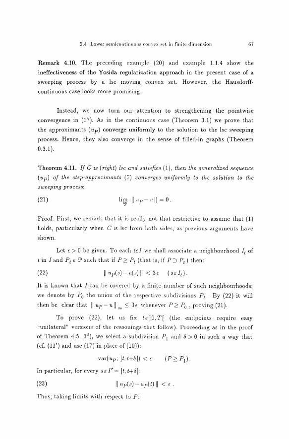
2.4 Lower semicoutinuons convcx sct iu finite clirnension 67

Remark 4.10. The preceding example (20) and example 1.1.4 show the

ineffectiveness of the Yosida regularizat.ion approach in the present case of a

sweeping process by a lsc moving convex set. However, the Hausdorff.

continuous case Iooks more promising.

Instead, we now turn our atteution to strengthening the pointwise

convergence m (17). As in the continuous case (Theorem 3.1) we prove that

the approximants (up) converge uniformly to the solution to the lsc sweeping

process. Hence, they also converge in the sense of filled-in graphs (Theorem

0.3.1).

Theorem 4.11. IJ Cis (rigid) lsc a.nd sa.tisfies (1), then the generalized sequence

( up) of the step-a.pproxim.a.nts (7) con·ucrges 1t.niformly to the solution to the

sweeping process:

(21) !im llup- u.ll = 0. ':)>

Proof. First, we remark that it is really not that restrictive to assume that (1) holds, particularly when C is lsc from hoth sicles, as previous arguments have

shown.

Let c > 0 be given. To eac!J tEl we shall ilssocia.te a ueighbourhood It of

t in I and Pt E 'P such that if P 2' Pt ( tha.t is, if P :=> P1 ) theu:

(22)

It is known that I can be covercd by a fiuite nnmber of such neighbourhoocls;

we clenote by P0 thc union of the respective subdivisions Pt . By (22) it will

then be clear that i11Lp- 1L II oc· :=:; 3 c w!Jenevcr P 2' P0 , proving (21 ).

To prove (22), Iet ns fix tc]O,T[ (the enclpoints require easy

"unilateral" versions of the reasonings tlwt follow). Procceding as in the proof

of Theorem 4.5, 3°), wc select a subclivision P1 ancl 8 > 0 in such a way that

(d. (11') and use (17) in place of (10)):

var(up; ]t.t+8]) < c

In particular, for every sEI*= ]t, t+8]:

(23) llup(s)-1tp(t) II < f.

Thus, taking Iimits with respect to P:

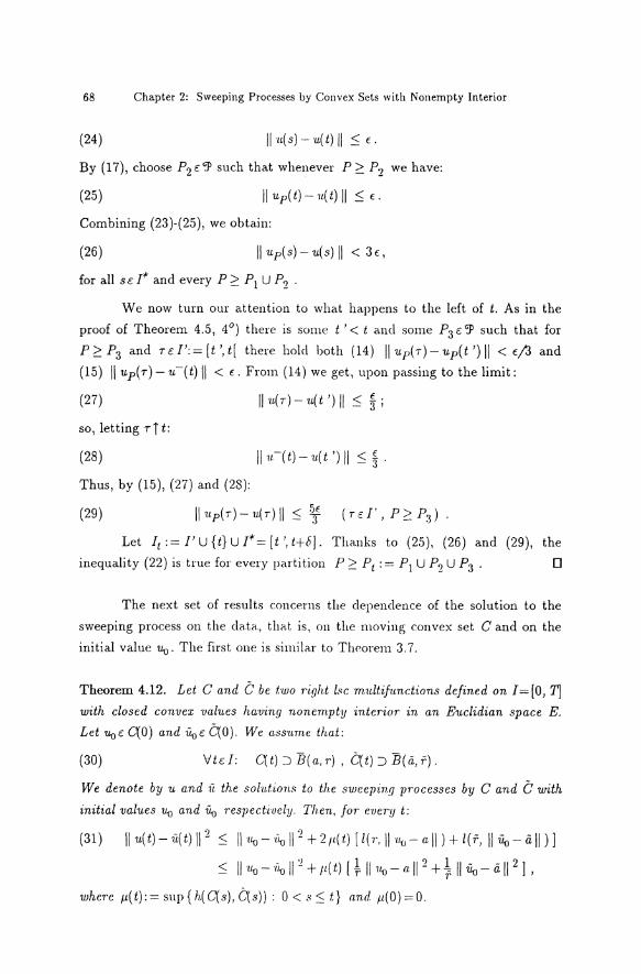
68 Chapter 2: Sweeping Processes by Convex Sets with Nonempty Interior

(24) llu(s)-·u(t)II:S:E. By (17), choose P2 c 'P such that whenever P:::: P2 we have:

(25) II u p( t)- u( t) II :::; c Combining (23)-(25), we obtain:

(26) llup(s)-u(sJII < 3E,

for all sc I* and every P:::: P 1 U P2 .

We now turn our attention to what happens to the left of t. As in the

proof of Theorem 4.5, 4°) there is some t '< t and some P3 c 'P such that for

P::::P3 and ui':=[t',t[ there hold both (14) llup(r)-up(t')ll < E/3 and

(15) II up( r)- u-( t) II < E. From (14) we get, upon passing to the Iimit:

(27) llu(r) -n(t ') II :S: ! ; so, letting r[ t:

(28) II ·u.-(tl -u.(t ') II :::; ! . Thus, by (15), (27) and (28):

(29) llup(r)-u(r)II:S:~ (rE.!',P::::P3 ).

Let I1 : = I' U { t} U I*= [ t ', t+b']. Thanks to (25 ), (26) and (29), the

inequality (22) is true for every partition P:::: P1 : = P1 U P2 U P3 . 0

The next set of results concerns tl1e clependence of the solution to the

sweeping process on the cla.ta, that is, on the moving convex set C and on the

initial value 'llo· The first one is similar to Tlworem 3.7.

Theorem 4.12. Let C and C be two right l8c multifnnctions defined on I=[O, T] with closed convex values having nonempty interior in an Euclidian space E.

Let Uoc C(O) and i4Jc C(O). We ass·nme tha.t:

(30) YtE.!: C(t):JB(a,r), C(t):JB(a,T).

We denote by n and fi the solntions to the sweeping processes by C and C with

initial valnes uD and i4J respectiuely. Then, for every t:

(31) II u(t)- ü(t) 11 2 < lluD- r/D 11 2 +2/t(t) [ l(r. II ·uv- a II) + l(r, II i4J- äll)]

< lluD- 1/D 11 2 + fl( t) [ ~ ll11v- a II 2 + ~ II i4J- ä II 2 ] ,

where f.L(l):= sup{h(C(s), C(s)): 0 < s :S: t} and f.L(Ü)=O.

2.4 Lower semicontinuous convex set in finite dimension 69

Proof. Similar to that of Theorem 3.7. Without loss of generality, we consider

t= T. We have, by (7) and (17), ·u(T)=lim':P nP,n(P) and ü(T)=lim':P üP,n(P)

(analogously defined). By Moreau' s inequality on projections into two convex

sets:

II Up i-l- Üp i-l 11 2 , ,

+2tL(t) ( II Up i-Up i-111 + II Üp i -Üp i-111); '- ' ' '

summing up and simplifying:

II uP,n(P)- üP,n(P) 11 2 ~ II Uo- Üo 11 2 + 2tL(t) [ var(up;I) + var(üp;I)].

These total variations are easily bounckd above, thanks to assumption (30),

Theorem 4.5 and (3.18). Takiug limits we obtain (31) fort= T. 0

Remark 4.13. More generally, we have

(32)

where M and Mare arbitrary upper bouncls of the total Variations of all the

approximants (up) ancl (üp)· But, at least by using this technique, we arenot

allowed to take M=var(u;I) a.nd M=va.r(ü; I) in (32). For instance, from the

vague (i.e., weak-*) convergence of the measures dup to d·u (cf. Theorem

0.2.2(ii)r it does not follow that va.r(up; I)= J I dup I converges to

var(u;I)= J I du I or equivalcntly that limsup var(·np;I) ~ var(u;I).

Theorem 4.12 implies tltc following corollary, which states m a more

direct way the continuous clependcuce of the solntious on the clata:

Corollary 4.14. Let C and C,. ( n;::: 1) be lsc mult~fnnctions from I= [0, T] to

closed convex sets with nonempty interior in an Buclid·ian space E. Let

un,oE C"(O) (n :::0: 1) be s?tch tha.t u 11 , 0 -> ·uuE C(O) a.nd denote by Un and u the

solutions to the sweeping processes by C11 and C with init·ial values un, 0 and Uo

respectively. Suppose that:

(33) lim[sup h(C11(t),C(t))]=O. 11 Iei

Then, ( u11 ) converges to n 1t.n:iformly on I.

Proof. We have already seen tha.t I cau bc partitionecl into a finite m1mber of

intervals Ii = [ ti-l, ti] (1 ~ i ~ p) such that, for some weil chosen closed balls:

70 Chapter 2: Sweeping Processes by Convcx Sets with Nonempty Interior

(34)

Writing J.ln = sup{h(C11(t), C(t)): td} ancl using (33), we choose no suchthat

J.ln-:=; r whenever n 2: n0 . If tc I;, then an inequality by Moreau (Prop. 0.4.5)

ensures that :

hence:

(35)

We prove that uniform convergf'nce holds on the first subinterval

I1 =[lo, t1]=[0, t1]. Given a positive <, the hypotheses show that there exists

n1 2: no such that for every n 2: n1 :

(36)

(37)

ll11·n ,o- 11{) II -::; €/V ,

fln [ 211 'llü- a1ll + €/V] 2 /r-:=; €2/2 . We apply Theorem 4.12 to C71 , C, u.n,o ancl ·uü, taking (34)-(37) into account,

and we obtain from (31) the estimate:

2 . . 2 1 2 1 2 llun(t)-u(tJII-:=; ll 11·n,o-ut.JII +Jln[rll·u.ll,O-a.JII +2riiUrJ-arll]

-::: <2/2 + Jln [ ( II uü- a., II + €/,[2 l2 + II Uv- ar ll 2 l/r -::: € 2 ,

that is,

(38) II ·u.n( t)- 11.( t) II -::; <

The uniform convergence of ( u11 ) to ·u. on I2 = [ t 1 ,t2] is obtained in the

same way because, by (38), the initial valnes at t=t1 satisfy un(t1)-4u(t1).

Thus, we consecutively establish the uniform convergence on each subinterval,

and hence on I. 0

Remark 4.15. The question of existence of a solution to the sweeping process

by a lower semicontinuous moving convex set with nonempty interior in an

infinite-dimensional Hilbert space arises naturally. Let us point out some of

the difficulties inherent in such a generalization to arbitrary climension.

a) Defining the net of approximants ('up) exactly as before, we can now extract

from it a subnet which converges pointwisely weakly to some bv function u

(see 0.2(8)). Reasoning as in the proof of Theorem 4.5, we have u(O) = Uv and

u( t) c C( t) ( tc I) but we are nnable to ohta.in the right-continuity of u (11) or

the condition (12) at jump points (strong pointwise convergence is needed).

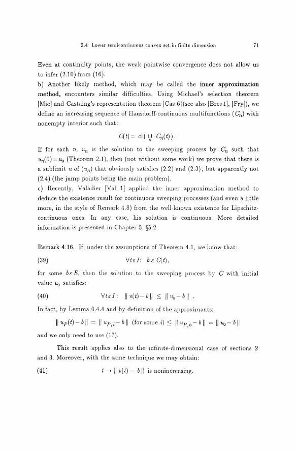
2.4 Lower semicontinuous convex sct in finite rlirnension 71

Even at continuity points, the weak pointwise convergence does not allow us

to infer (2.10) from (16).

b) Another likely method, which may be called the inner approximation

method, encounters similar clifficulties. Using Michael's selection theorem

[Mic] and Castaing's representation theorem [Cas 6](see also [Bres 1], [Fry]), we

define an increasing sequence of Hausclorff-continuous multifunctions ( C11 ) with

nonempty interior such that:

C( t) = cl ( U Cn( t)) . n

If for each n, 1Ln is the solution to the sweeping process by Cn such that

u11(0)=Uo (Theorem 2.1) 1 then (not without some work) we prove that there is

a sublimit u of ( v.n) that obviously satisfies (2.2) ancl (2.3) 1 but apparently not

(2.4) (the jump points being the main problem).

c) Recently, Valaclier [Val 1] appliecl tl1e inner approximation method to

deduce the existence result for continuous swecping processes (and even a little

more, in the style of Remark 4.8) from the well-known existence for Lipschitz­

continuous ones. In any case 1 his solution is continuous. More detailed

information is presentecl in Chapter 51 §5.2.

Remark 4.16. If, under the assumptions of Theorem 4.1 1 we know tha.t:

(39) Vtd: b E C(t) 1

for some bE E 1 then the solntion to the sweeping process by C with initial

value Uo satisfies:

( 40)

In fact, by Lemma 0.4.4 ancl by clefinition of the approxima.nts:

and we only need to use (17).

This result applies also to the infinite-dimensional ca.se of sections 2

and 3. Moreover, with the same technique we ma.y obta.in:

( 41) t ---. !Iu( t) - b II is nonincreasing.

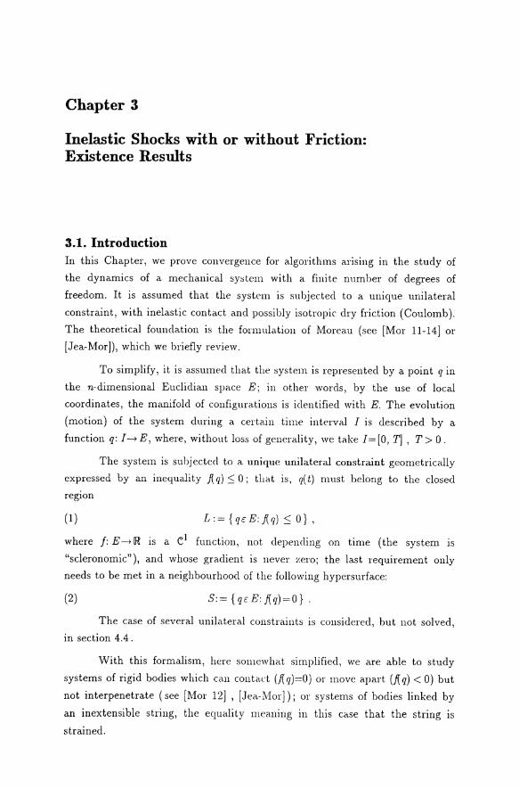
Chapter 3

Inelastic Shocks with or without Friction: Existence Results

3.1. Introduction In this Chapter, we prove convergence for algorithms ansmg in the study of

the dynamics of a mechanical sy~tem with a finite number of degrees of

freedom. lt is assumed that the system is subjected to a unique unilateral

constraint, with inelastic contact and possibly isotropic dry friction (Coulomb).

The theoretical founclation is the fonnulation of Moreau (see [Mor 11-14] or

[Jea-Mor]), which we briefly review.

To simplify, it is assumed that the system is represented by a point q in

the n-dimensional Eucliclian space E; in other worcls, by the use of local

coordinates, the manifolcl of configura.tions is identified with E. The evolution

(motion) of the system cluring a certain time inte1·val I is described by a

function q: I-+E, where, without loss of generality, we take l=[O, T], T> 0.

The system is subjected to a unique unilateral constra.int geometrically expressed by an inequality fi.. q) S 0; that is, q( t) must belong to the closed

region

(1) L:= {qt:E:.f{q) S 0},

where f: E---+ IR is a e1 function, not depending Oll time ( the system is

"scleronomic"), and whose gradient is never zero; the last requirement only needs to be met in a neighbourhood of the following hypersurface:

(2) S:={qt:E:fi..q)=O}.

The case of several unilateral constraints is considered, but not solved,

in section 4.4 .

With this formalism, here somewhat simplifiecl, we are able to stucly

systems of rigid hoclies which can contact (fi..q)=O) or move apart (fi..q) < 0) but

not interpenetrate ( see [Mor 12] , [Jea-IVIor]); or systems of hoclies linked by

an irrextensible string, the equa.lity meaning in this case that the string is

strained.

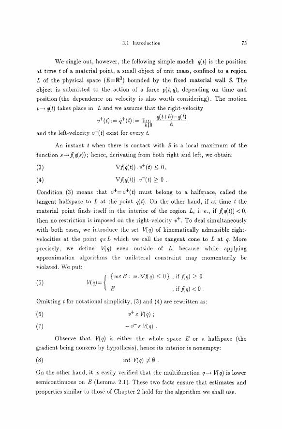
3.1 lnt.roduction 73

We single out, however, the following simple model: q(t) is the position

at time t of a material point, a small object of unit mass, confined to a region

L of the physical space (E=IIi!3) bounded by the fixed material wall S. The

object is submitted to the action of a force p( t, q), depending on time and

position (the dependence on velocity is also worth considering). The motion

t-; q( t) takes place in L and we assume that the right-velocity

v+(t) := q+(t) := lim q(t+h)-q(t) hlO h

and the left-velocity v-( t) exist for every t.

An instant t when there is contact with S is a local maximum of the

function s-; f{ q( s)); hence, derivating from both right and left, we obtain:

(3)

(4)

'Vj(q(t)). v+(t) :::; 0,

'VJ(q(t)). v-(t) ~ 0 .

Condition (3) means that v+ = v+( t) nllist belong to a halfspace, called the

tangent halfspace to L at the point q( t). On the other hand, if at time t the

material point finds itself in the interior of the region L, i. e., if f{q(t)) < 0,

then no restriction is imposed on the right-velocity v+. To deal simultaneously

with both cases, wc introduce the set V( q) of kinematically admissible right­

velocities at the point qc L wllich we call the tangent cone to L at q. More

precisely, we define V( q) even outside of L, because while applying

approximation a.lgorithms the unilateral constra.int may momenta.rily be

violated. Wc put:

(5) { {wo:E: w.'V.f(q):::; 0}, if.f(q) ~ 0

V(q)= E , if f{ q) < 0 .

Omitting t for notational simplicity, (3) and (4) are rewritten as:

(6)

(7)

·v+ E V( q) ;

-11-E V(q).

Observe that V( q) is either the whole spa.ce E or a halfspace ( the

gradient being nonzero by hypothesis), hence its interior is nonempty:

(8) int V( q) =/0 .

On the other ha.nd, it is easily verifiecl that the multifnnction q-; V( q) is lower

semicontinnous on E (Lemmil. 2.1 ). These two facts ensure that estimates and

properties similar to those of Chapter 2 lwld for the algorithm weshall use.

74 Chapter 3: lnelastic Shocks with or wit.hout Friction: Existence Results

If an episode of smooth motion ends at the instaut t with left-velocity

v- E. V(q), that is, if J(q)=O and v-. \lf(q) > 0 then a shock necessarily occurs:

right-velocity is different from left-velocity.

Let us consider first the case of a perfect frictionless contact. The

material point (system, body) then experiences from the part of the "wall" S a

normal reaction force r, pointing inwards to L a.t the contact point q. In other

words, r is suchthat ([Mor 11] (2.2)-(2.3); [Mor 12] (3.7)-(3.8)):

(9)

(10)

3 .>.ciR: r=->.'VJ(q);

). ~ 0 .

This inequality expresses the absence of adhesion to S. By "integrating" the

reaction (or liaison) force r "for the (infinitesima.lly sma.ll) duration of the

shock" and assuming that r does not change direction, we obtain the Iiaison

percussion P. Thanks to (9) ancl (10), P satisfies ([Mor 12] (5.1), (5.2)):

(11) P= v+- v- = -a\lf(q) (a > 0).

Conditions (6) and (11) alone do not univocally determine v+, the

velocity after the shock, once the velocity before the shock v- is known. We

say that it is an ela.stic shock if the (kinetic) energy is conserved; that is, if:

(12)

in the euclidian norm of E, which is chosen so that the kinetic energy is given

by

(13)

Taken together, (11) and (12) imply that v+ is obtained from v- by

geometrical reflection with respect to the tangent hyperplane to L at point q.

The other idea.! extreme case, which is the. object of this study, is that

of a soft or inela.stic shock: the velocity after the shock is tangential, i. e.,

(14) v+.\lf(q)=O.

Accounting for (11), it is geometrically clear that v+ JS the orthogonal

projection of v- into the tangent hyperplane

(15) T(q)={w: w.\lf(q)=O};

in particular,

(16)

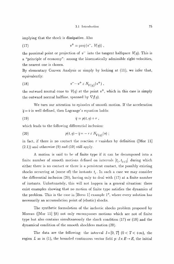
.3.1 Introduction 75

implying that the shock is dissipative. Also

(17) v + = proj ( v-, V( q)) ,

the proximal point or projection of v- into the tangent halfspace V( q). This is

a "principle of economy": among the kinematically admissible right-velocities,

the nearest one is chosen.

By elementary Convex Analysis or simply by looking at (11), we infer that,

equivalently:

(18)

the outward normal cone to V( q) at the point v+, which in this case is simply

the outward normal halfline, spanned by V./( q).

We turn our attention to episodes of smooth motion. If the acceleration

ij = iJ is weil defined, then Lagrange' s equation holcls:

(19) 'rj = p( t, q) + r ,

which Ieads to the following differential inclusion:

(20)

in fact, if there is no contact the reaction r vanishes by definition ((Mor 11]

(2.1)) and otherwise (9) ancl (10) still apply.

A motion is said to be of finite type if it can be clecomposed into a

finite number of smooth motions ddined on intervals ]ti, ti+l[ during which

either there is no contact or there is a persistent contact, the possibly existing

shocks occurring at (some of) the instants ti. In such a casc we may consider

the differential inclusion (20), having only to deal with (17) at a finite number

of instants. Unfortunately, this will not happen in a general situation: there

exist examples showing that no motion of finite type satisfies the dynamics of

the problem. This is the case in [Bress 1] example 1°, where every solution has

necessarily an accumulation point of (elastic) shocks.

The synthetic fonnulation of the inelastic shocks problern proposed by

Moreau ([Mor 11] §8) not only encompa.sses motions which a.re not of finite

type but also contains simultaneously the shock conclition (17) or (18) and the

dynamical conclition of the smooth shockless motion (20).

The clata are the following: the interval 1=[0, T] (0 < T< +oo), the

region L as in (1 ), the bounded continuous vector field p: /x E ~ E, the initial

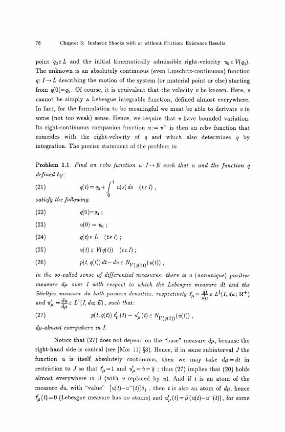
76 Chapter 3: Inelastic Shocks with or wit.hout Friction: Existence Results

point q0 t:: L and the initial kinematically admissible right-velocity 11u € V( q0 ).

The unknown is an absolutely continuous (even Lipschitz-continuous) function

q: I-tL describing the motion of the system (or material point or eise) starting

from q(O)=q0 . Of course, it is equivalent that the velocity v be known. Here, v

cannot be simply a Lebesgue integrable function, defined almost everywhere. In fact, for the formulation to be meaningful we must be able to derivate v in

some (not too weak) sense. Hence, we require that v have bounded variation.

Its right-continuous companion function u:= v+ is then an rcbv function that coincides with the right-velocity of q and which also determines q by

integration. The precise statement of the problern is:

Problem 1.1. Find an rcbv function u: I-tE such that u and the function q

defined by:

(21) q(t)=q0 + jt 11.(s)ds (td), 0

satisfy the following:

{22)

(23)

(24)

(25)

(26)

q(O)=qo;

u(O) = Uo;

q(t)t:: L (tt:: I);

u( t) € V( q( t)) ( t € I) ;

p(t, q(t)) dt- du e NV(q(t))(u(t)),

in the so-called sense of differential measures: there is a ( nonunique) positive

measure dtt over I with respect to which the Lebesgue measure dt and the

Stieltjes measure du both possess densities, respect·ively t'Jl = jt c: L 1(I, dp.; IR+) and u~ = ~; € L 1(I, du; E), such that: fL

(27) p(t, q(t)) ~1 (t)- ·u~1 (t) e NV(q(t))(u(t)),

dtt-almost everywhere in I.

Notice that (27) does not depend on the "base" measure dtt, because the

right-hand side is conical (see [Mor 11] §8). Hence, if in some subinterval J the

function u is itself absolutely continuous, then we may take dtt = dt in

restriction to J so that t'll = 1 ancl ·n~1 = u = ij ; tlms (27) implies that (20) holds

almost everywhere in J (with v repla.cecl by u). And if t is an atom of the

measure du, with "value" [1L(t)-u-(t)]b'1 , then t is also an atom of dtt, hence

t'll ( t) = 0 (Lebesgue measure has no atoms) ancl u~ (t) = ß ( u( t)-u-(t)), for some

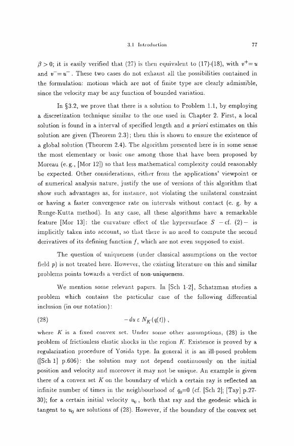
:).1 lntroduction 77

ß > 0; it is easily verifiecl that (27) is then equivalent to (17)-(18), with v+= u

ancl v-= u-. These two cases do not exhaust all the possibilities contained in

the formulation: motions which are not of finite type are clearly admissible,

since the velocity may be any function of bounded variation.

In §3.2, we prove that there is a solution to Problem 1.1, by employing

a discretization technique similar to the one used in Chapter 2. First, a local

solution is found in a interval of specified length and a priori estimates on this

solution are given (Theorem 2.3); then this is shown to ensure the existence of

a global solution (Theorem 2.4). The a.lgorithm presented here is in some sense

the most elementary or basic one among those that have been proposed by

Moreau (e. g., [Mor 12]) so that less mathematical complexity could reasonably

be expected. Other considerations, either from the applications' viewpoint or

of numerical analysis nature, justify the use of versions of this algorithm that

show such advantages as, for instance, uot violating the unilateral constraint

or having a faster convergence rate on intervals without contact (e. g. by a

Runge-Kutta method). In any case, all these algorithms have a remarkable

feature [Mor 13]: the curvature dfect of the hypersurface S - cf. (2)- is

implicitly taken into account, so tha.t thcre is no ncccl to compute the second

derivatives of its defining function /, which arenot even supposed to exist.

The question of uniqucness (und er classical assumptions on the vector

field p) is not treated here. However, the existing literatme on this and similar

prohlerns points towards a verdict of non-uniqueness.

We rnention some relevant papers. In [Sch 1-2], Schatzman studies a

problern which conta.ins the particular case of the following differential

inclusion (in our notation):

(28)

wherc K is a fixed convcx sct. Undcr some othcr assumptions, (28) is the

problern of frictionless ela.stic shocks in thc region K. Existence is proved by a

regularization procedure of Yosicla type. In general it is an ill-posed problem

([Sch 1] p.606): the solution may not depend continuously on the initial

position and velocity and moreovcr it rnay not be unique. An example is given

there of a convex set K on the boundary of which a certain ray is reflected an

infinite nurnber of tirnes in the neighbourhoocl of q0=0 ( cf. [Sch 2]; [Tay] p.27-

30); for a certain initial velocity Uo , both that ray and the geodesie which is

tangent to Uo are solutions of (28). However, if the boundary of the convex set

78 Chapter 3: Inelastic Shocks with or wit.hout Friction: Existence Results

is of dass e2 and its gaussian curvature is strictly positive everywhere, then

the solution is unique and of finite type ([Sch 1] Theorem 2, generalized in [Per]). Another type of nonuniqueness is given by Bressan in [Bress 1],

example 3, and in [Sch 3] there is an example even for L= [0, +oo[. Buttazzo and Percivale treated this kind of problem by means of r-convergence [But­

Per 1-2). A discussion of uniqueness and regularity is found in [Bress 3,4).

Among the many papers dealing with the related question of unilateral

contact between deformable bodies, hence with infinite number of degrees of

freedom, let us ci te [ Ame-Pro] on the vi brating string in the presence of an

obstacle (where nonuniqueness is again possible (Cit]) and [Do] on the

longitudinal dynamics of a bar whose end bumps against an obstacle.

En passant, let us note that several second-order differential inclusions

are treated in the literature; for instance, the following hyperbolic one is a

particular case of [Bar]V.l.l :

(29) - ~~ t: M(u(t)) + A(q(t)),

where M is a fixed time-independent nonlinear monotone multifunction and A is a continuous symmetric linear operator.

Problem 1.1 applies to all situations where it is reasonable to neglect

frictional effects. If this is not the case, the friction usually present at contact

must be incorporatecl in the ana.lysis. This will be clone by adopting the

formulation of Moreau, especially in [.Mor 12] §§ 11, 12.

The classical isotropic Coulomb's law of friction is assumed to hold. To

each point qt: S is associated the so-called fridion cone C=C( q). This is a cone with vertex at the origin and revolving about the inward normal to L at the point q with an angle a(q) t: ]0,7r/2[. The inequality a(q) < 1r/2 means that friction is finite in every direction. Iutroducing the notation

(30) \7 f{ q)

n=n(q)==- II \lf{q) II ' we may describe the friction cone as:

(31) C=C(q)={vt:E: v.n(q)? ii·uiicosa(q)}={vt:E:-v.\lf{q)? c(q)llvll },

where c( q): = II \7 f{ q) II cos a( q) is a real funrtion, positive on Sand continuous

by hypothesis. Without significant loss of generality, we even assume that c(q)

is defined, positive and continuons on thc~ whole spa.ce E.

3.1 In trod uction 79

The friction law stipulates the following:

1 °) The reaction force r belongs to the friction cone:

(32) TE. C;

in particular, it is directed towards the interior of the region L, which means

that there is no adhesion effect.

2°) If there is no contact, then there is no reaction:

(33) J(q) < 0 =} r=O .

3°) If u= g_+ is the right-velocity, then:

(34) u. n > 0 =} r= 0 ,

because in this case the contact necessarily ceases in some time-interval to the

right of the considered instant, hence, by (33), r= 0 on that interval and the

same is true for the right-limit of r.

4°) If u.n=O, that is if 1L belongs to the tangenthyperplane T= T(q), then

the classical form of the friction law is equivalent to the new condition (see

[Mor 12] (11.15) and pp. 75-76):

(35) 1L. n = 0 =} - ·u [. proj T N c( 1') '

the orthogonal projection into T of the outwa.rcl normal conc to C a.t r.

This formula.tion is rema.rka.ble namely for a handoning the usual

decomposition of the reaction into its normal and tangential components.

Notice also tha.t (35) only cletermines the clirection of r: any Ar with ,\ > 0 will

also satisfy (35). This fact is essential to the statement of the problern in terms

of differential measures, as presentecl next.

From La.gra.nge' s equation ( 19), tl1at is, from r= du/dt- p( t, q) it follows

that rdt = du- p( t, q) dt holds in the sense of measures, in every subinterval

where u is smooth. Let us introduce a vector measure which can be called the

reaction measure:

(36) dR=du-p(t, q(t))dt.

We see that r ma.y be replacecl in (32)-(35) by the clensity

(37) ~~ = ddR t: L1(I, dJt; E) , ·ll

where dj.L is a.ny positive mea.sure with respect to which dR IS absolutely

continuous. The sought-for matlwmatica.l formula.tion is then:

80 Chapter 3: Inelastic Shoc.ks with or without Friction: Existence Results

Problem 1.2. Given q0 E L a.rul uv E V( q0 ) , find an rcbv ftmction ( the right­

velocity) u: I-+ E defining a Lipsch:itz-contintwus. motion q: I-+ E by integration

(38) q(t)=q0 +jtu(s)ds (tel), 0

in such a way that:

(39) q(O) = qo ;

(40) u(O) = Uo;

(41) q(t)c. L (tc. I);

(42) u(t) E V(q(t)) (tc. I);

and the following implications n.re tr·u.e dtt-almost everywhere:

(43) f{q(t)) < 0 => r'l'(t)=O;

(44) [f{q(t))=O, u(t). \lj{q(t)) < 0] => 1~1 (t)=0;

(45) [f{q(t))=O, u(t). \lj{q(t))=OJ =>- ·u.(t)c. projT(q(t)) NC(q(t))(r'l'(t)),

where dp. is any positive mea.sure on I such that ~~ can .be defined by (36) and

(37).

Notice that (45) implicitly reqmres that r'l'(t)c.C(q(t)), dp.-almost

everywhere. In case of a shock at time t, the measure dR has an atom at t that

equals (u(t)-u-(t))8t and t is also an atom of the positive measure dp.; since

its right-hand siele is a cone, ( 45) is equiva.lent to

(46)

which in turn is equivalent to the following (see [Mor 12], p. 78-79)

(47) ·u(t)=proj (0, [u.-(t)+C{q(t))]n T(q(t))).

The algorithm of approximation developed in §3.3 is based on the last

condition (see (3.8)). Under the additional a.ssumption that the gradient of f is

a Lipschitz-continuous function of q, it is proved tha.t there exists a solution to

Problem 1.2 ( defined on I). This is tedmically more difficult than the

frictionless case. Let us point out that ( 45) is replaced by a "user-friendlier"

"variational" condition (Lemma 3.13).

Also in this case, we shall not discuss uniqueness or non-uniqueness of

solutions, when the force p is Lipschitz-continuous with respect to q. It has

:3.1 lnt.roduction 81

long been recognized that, when dealing with the dynamics of systems with

dry (Coulomb' s) friction, the uniqueness of the motion for certain initial

values cannot be ensured [Del 2] [Löt 2] [Bress 2]. This question is linked to the

uncertainty concerning the contacts that cease [Del 1] and to the occurence of

shocks namely the so-called tangential shocks ( cliscontinuities of velocity after

smooth motion episocles and without new contacts appearing); here, we refer

of course to the more general case of several unilateral constraints .h ( q) :S:: 0. In

[Del 2] are given some examples where the only possible motions are those

with shocks; see also [Löt 2] and [Jea-Pra], last section. Stick-slip phenomena

appear e. g. in [Jea-Mor] §§ 6, 8.

These difficulties prompted vanous authors to find conditions under

which the system does not experience any shocks or cloes not lose contact, at

least in the beginning of the motion {for instance, [Jea-Pra] [Del 2]). Then,

existence and uniqueness can be establishecl [.Jea-Pra]: the normal component

of the reaction is taken as the unknown ancl a fixecl-point technique is usecl to

solve a quasi-variational inequality. A smooth behaviour of the solution is also

implicitly assumed a priori in [Löt 2], where an algorithm ancl a local existence

result are given. Let us mention other works in this active research field. In

[Löt 1], the emphasis is put on the numerical aspects without studying

existence. In [Löt 3] a less direct algorithm {involving the explicit computation

of some Lagrange multipliers) is exhihited for the motion of a bidimensional

system with unilateral contacts. In [.Jea] is consiclerecl a pla.ne obstacle and a

motion with persistent contact of a system of points, which allows some

simplifications in the algorithm. In [Rio 1, 2] we may find an existence result

for the unidimensional case (one degree of freeclom). In [Mau] the normal

component is assumed to be known as a function of time. Algorithms are also

presented in [Tau 1, 2].

From the theoretical point of view, Curnier shows in [ Cur 1] the same

concern for a coherent formulation, in a setting that goes beyond Coulomb' s

friction, but restrictecl instead to small displacements. Another line of research

arises when Clarke' s normal cone is substituted for the usual cone as in the

works [Pan 1, 2].

To end this introcluction, let us stress that the numerical techniques

proposed by Moreau, namely in [Mor 12], ancl usecl here, overcome some of the

past difficulties in that they deal simultaneously with: 1) the nondifferentiable

82 Chapter 3: Inelastic Shocks with or without. Frictiou: Existence Results

relations induced by the dry friction and the unilaterality of the constraint

( which are physically related features) and 2) smooth motion episodes and

shocks and even possibly duster points of shocks.

3.2. Frictionless inelastic shocks The region L is defined by (1.1 ), that is, by the inequality .!( q):::; 0, where

f: I->IR is a e1 function.with nonzero gradient. We prove the following simple

property:

Lemma 2.1. The multifunction q-> V( q), the tangent cone to L at q ( see (1.5 )) 1

is lower semicontinuous ·in E and ha.s closed convex values with nonempty

interior.

Proof. In the interior of L, the multifunction V is lsc because it is constant,

equal to E. Let .!( q0 ) ~ 0 ancl U be an opeu set that intersects V( q0 ) ancl hence

also the interior of this set. If vve take vr:: U suchthat v. \l.f(q0 ) < 0 , then, by

continuity of the graclient, we may find a. ueighbourhoocl W of q0 ensuring that

V. \l.f(q) < 0 for all qc w' whence un V(q) -10 . 0

To avoicl unessentia.l technical clifficulties, we sha.ll assume that the

external forces satisfy the following assumption.

Assumption 2.2. The contin1t.ons vecto1· field p: I x E-> E is globally bounded1

i. e. 1 there is a. consta.nt M > 0 such thn.t:

(1) //p(t 1 q)//:::; M (tel, qE E).

Theorem 2.3. (Existence of a local solution) Let q0 c L and Uo c: V( q0 ) be the

initial data for t=O. By Lemmas 2.1 and 2.4.2, we take 8 > 0 such that:

(2) int( V(q) )-f 0

and T 1 > 0 defined by:

(3) T 1=min{T, ~,}, M'= /lu0 /l +2TM.

Then1 on the interval I 1 : = [0, T '] 1 Problem 1.1 has at least one solution q with

3.2 Frictionless inda.stic shocks 83

right-velocity u that sat-isfies:

(4) II u(t) II < II·~~ II +Mt

(cf. [Mor 11] §8) and so by (1.21):

(5) II q( t) II :::: II qo II + II Uo II t + ! Mt 2 .

The existence of a global solution is then easily deduced:

Theorem 2.4. (Global existcnce thcorem) The frictionless inelastic shocks'

Problem 1.1 has at least one global solution, th.at is, a sol1dion defined on the

interval I=[O, T].

Proof. We shall prove that T belongs to the set J of all the S in I for which

there exists a solution u5 , q8 of (1.21)-(1.27) clefined on [0, S]. In fact, we show

that J equals I, because it is a. nonempty dosed-open subset of I.

By the preceding Theorem, T 'E J and every solution u5 , q5 can be

continued to the right of S (the theorem is a.ppliecl with initial instant t=S

instead of t = 0, which is irrelevant), so J is open.

In order to show that J is closed, consider a sequence ( Sk) in J

converging to S a.ncl assmne that Sk < S for all k ( otherwise, the limit S

belongs trivially to J). Then, by (5), all the solutions qk, clefinecl on [0, Sk] and

with right-velocities v.k , satisfy the estimilte:

II qk(t) II :::: II qo II + II "~~ II S+ 1MS2 ;

in particular, the sequence of fina.l Ya.lues r/: = qk( Sk) is bounded in E. Let 7j

be a sublimit of ( r/) ancl choose [,* > 0 and an integer k such that:

(6)

(7)

(8)

int( n V(q) ) 7' 0; II q-q II ::: 2v

lll- q II :::: o* ;

s:::; sk + (\* [ ll·uü II + M(S+2 T)]- 1

From (6) and (7) it follows that

int( n II q-lll :::: o·

V( q) ) 7' 0 .

By Theorem 2.3, there is a solutiou q, with velocity il. a.nd with initial values

84 Chapter 3: lnelastic Shocks with or without Friction: Existence Results

ij(Sk) = / and ü(Sk) = uk: = ·uk(Sk), which is defined in the interval

[Sk, min{T, Sk+8*( II uk II +2 TM)- 1} J.

By (4), II uk /1 S: II Uo II + l\1Sk S: II Uo II +MS. Thus, it is clear from (8) that

the above interval contains [Sk, S]. Hence qk and uk can be continued, by

using ij and ü, to give a solution to the inelastic shocks problern which is

defined in [0, S]; i. e., Sc J and J is closed. 0

The proof of Theorem 2.3 will be done in several steps. We begin by

constructing a sequence ( u71 ) of approximants of the velocity and the

corresponding sequence ( q11 ) of approximants of the motion, all defined in the

interval I'. For each positive integer n, let us take h(=h71 )= T'jn and

t71 i = i/h= iT '/n (0 S: i S: n) and let us introduce two finite sequences ( q71 ;) ' , and ( u11 ;) of elements of E: ,

(9) qn,o = qo ;

(10) Un,o =proj (111J + hp(t11 ,o, (}11 ,o), V(qn,o));

(11) qn,i+l = qn,i+ h un,i i

(12) un,i+l = proj(11.n,;+hp(t",i+l, q11 ,i+l), V(qn,i+l)).

Then, we define Un by:

(13) if tt:[tn i, tn i+tf with 0 S: i S: n- 1 , , ,

and u71(T ') = u 71 , 11 • We define q11 by integration:

(14) q11(t) = q0 + jt n"(s) ds. 0

Several properties follow from the definitions above. Notice that:

(15)

From (12) and (1) we know that:

1/un,i+ll/ S lfun,i+hp(tn,i+l•qn,i+l)/1 S lfun,;lf+hM;

and by induction we obtain from ( 10):

(16) llun,J S: /1111)11 +(i+1)hMS: M':= 1f111lll +2TM.

By (2) there can be found a fixed cbsed ball B( a, r) which is contained

in every V(q) provided that II q-q0 II S: 8. Sin('(:' (13), (14) and (16) imply that

3.2 Frict.ionless irwlast.ic shocks 85

(17) 1111-11(s) II ds ~ M't ~ M'T' ~ 5,

it follows from (15) that:

(18)

Le=a 2.5. (a) The total varia.tion of un in [0, t] is bounded above according

to:

(19)

(b)

(20)

. 1 2 M2 2 1 var(n,vO, t) ~ 2r ( llnn,o- a II + hM) + 2r t + Mt(1 +r llnn,o- a II).

There is a constant c > 0 such tho.t:

Vnd\J : var( 11. 11 ; I) ~ c .

Proof. Lemma 0.4.4 (equation 0.4(6)) <~nd conditions (12) and (18) give

llnn,i+l-all ~ ll 11·n,;+hp(t11,i+l,q11,i+l)-all ~ II 1L11,;-all+hM, hence, by induction:

(21) llun,;- 11·11 ~ lln11,0-·all +Mtn,i ·

By the same argument, we deduce from (10) tltat:

(22) llun,o-all ~ ll·uv+hp(O,qu)-a.ll ~ II11D-a.II+Mh.

Writing w = 1L11 , 0 + h p( 111 , 1 , q11 , 1) we prove that, for all i,

2 1 •) ? L llun,j-un,j-111 ~ 2r(llw-all--ll·nn,i-a.1!-) j=l Jyj! 2 1

+ 21--t11,i +Mt",;(1+rllnn,o-a.II)-

(23)

If i = 1, we simply apply Lemma 0.4.3; sinn~ ·un, 1 = proj ( w, V( qu, 1)) and

B( a, r) C V( q11 , 1) (by (18)), we haw:

II un, 1- Un,o II ~ 11 11·11 , 1- ·w II + II w- Un,o II

~ ir( 11 111 - a 11 2 - 111Ln, 1- a 11 2) + Mh.

Assuming that (23) holds by indnction, we remark that, for similar reasons, in

the next step:

II un,i+l- un,i II ~ ir( 111Ln,i + hp(tn,i+1 • rJn,i+1)- a 11 2 - ll·un,i+1- a 11 2)

+Mh;

whence, by (21):

86 Chapter 3: Inelastic Shocks wit.h or wit.hout friction: Existence Results

1 2 2 2,,( II n",;- a.ll -II nn,i+l- a.11 )

lvf2 2 1 + 2T ( h + 2 h tn) + M h ( 1 + r II Un, 0 - a II ) .

Adding this inequality to (23) we obtain the formula corresponding to i+l

( because t11 } + h2 + 2 h t11 , ;= (t11 , i + h)2 = t11 , i+l2 ) and this establishes the

result.

(a) Let now tt:Iand consicler the integer ifor which tt:[t11 ;,t11 i+l[. By (23): . ' , l

var(u11 ;0,t)=?:: llu",j-un,j-JII ;=1 ~ 1 ·) M- ·) 1 S 2,, II w - a. II - + 2 r t- + Mt ( 1 + r II un, o - a II ) ;

and, since II w- a II S II V71 , 0 - a.ll + hM, we get (19).

(b) In particular, take t= T' in (19) ancl take account of (22) and h S T '.

Then it is clear that (20) is sa.tisfied, with e. g.

c=Jr(llno-all +2MT')2+J:f2 T'2 +MT'[1 +t(ll1t'O-a.ll +2MT')J. D

The sequence of Lipschitz-continuous functions ( q") is equicontinuous,

as a consequence of (13), (14) ancl (16):

(24) II q11(t)- q11(s) II II j 1 u,,(r)dr II s M' I t- sl . s

Moreover, for every n:

(25) q11(0) = qo ·

Thus, by Ascoli-Arzela's Theorem, (q11 ) is a relatively compact sequence for

the uniform con vergence topology. W e prove that any sublimi t of ( qn) is a so1ution in I' to the frictionless inelastic shocks' problcm.

Consider then a function q: I'-+ E such that:

(26) !im q11 ( t) = q( t) 'j

uniformly in I', where :f is some increasing sequcnce of positive integers. Since

( Un) is uniformly bounded by M' and it is bouncled in total variation (Lemma

2.5(b )), it follows by Theorem 0.2.1 that it is relatively compact for pointwise

convergence. So, replacing :f by a subsequence if need be, we may assume that:

(27)

where v is a bv fuuction.

\ftt: I': !im u71 ( t) = v( t) , 'j

3.2 frictionles;; inelastic sl10cks 87

vVe define u:= v+, the right-limit of ·u. By tl1e clominated convergence

theorem, (14) and (26)-(27) yield:

(28) q(t) = q0 + jt v(s)ds= q0 + j 1 11.(s)ds, 0 0

i.e., (1.21) and hence (1.22). Postponiug the proof of (1.23), we now show that:

Proposition 2.6. Every q( t) with tc; I' belongs to L, that is:

(29) fi.q(t)) ~ 0 (td ') .

Proof. Let K be an upper bouncl of the norm of the graclient of f in the ball

B ( q0 , 8) and define for every p > 0 :

ry(p):=max{ IIVfi.q)-\lj{q')ll q,q'd3(qo,8)' llq- q'll ~p} ·

Since the gradient of f is uniformly continnons in the consiclered ball, we have:

lim 7J(p)=O. p~O

The next inequa.lity measures m ~ome sense the violation of the

unilateral constraint committecl by the approximant q11 • If tc[O, t 11 ;J, then: '

(30) T' fi.qn(t)) ~ hM'K+t11 ,;M'1J(hM'), h=n

If i= 0, this is trivial because q11 (0) = q0 E L. Assuming that (30) holcls by

incluction, we next consicler an arbitrary t::: ]t1 ·, t 7·+ 1] . 1,t n,

If fi. q11 i) ~ 0, then by (16) and (17):

' Jt t f{q11(t))=f{q11 )+ 1 _Vfi.qn(s)).1L11(s)ds ~ j 1 .11 \lf{q11(s)) II

n,z n,z IIUn(s)ll ds

~ hKM',

whence (30).

On the other hand, if fi. q11 , ;) > 0, then 11 71 , i. \7 fi. q11 , ;) ~ 0, by construction. We

notice also that if sE[tn,;,t] then II q71(s)- q11 ,,:ll =(s- tn) llu",;ll ~ hM'.

Since 77 is nondecreasing, using the incluction hypothesis ancl (15)-(17) we have:

Jt t f{q11(t))=f{q") + t . \7f{q11 ). ·un,i ds+ j t . [\l.~q11 (s))- \7f{q11 )]. un,i ds

n,z n.,1.

~ fi.qn)+M' ;: . 77( II qn(s)- q11 ,; II )ds n,z

~ [hM 'K + tn ;M '17(hM ')] +M 'h17(h.M ') = hM 'K + t .+1M'ry(hM'), , n, z

which proves (30) in [O,tn,i+Jl.

88 Chapter 3: Inelastic Shocks with or without Friction: Existence Results

Taking limits as n--->oo with nt:f in the inequality (30), we obtain (29)

because t11 i:::; T', h= T'/n--->0 and therefore 7J(hM')--->0. D '

We have just established (1.24) q(t)c: L, which implies (see (1.6)) that

(1.25) u( t) c; V( q( t)) holds for every t in I' with the possible exception of T '; for

the right endpoint we adopt the convention:

(31) u(T')=v+(T'):= proj(v-(T'), V(q(T'))).

The next result is essential in order to prove (1.26) and (1.27) at

continuity points of u and v.

Lemma 2.7. Let 0 :::; s :::; t < T' and a.ssume that zc: V(y) for every y in some

neighbourhood of the set q([ s, t]). Th.en:

(32) z.(v(t)-v(s)) 2:: ~( II v(t) 11 2 - II v(s) 11 2) + jt (z-v(r)).p(r,q(r))dr. s

Proof. The uniform convergence in (26) ensures that for n large enough the set

q11([s, t]) is contained in the saicl neighbourhood of q([s, t]). In particular, if the

nodes of the partition tha.t belong to ]s, t] are tn,j < tn,j+l < ... < tn,k (j and k

vary with n) then zc: V( qn,;) (j:::; i:::; k). Since u11 , i is the projection of

uni-l+hp(t11 i,qni) in V(q71 i), then, by the well-known property of ' ' ' '

projections, we may write:

Adding up these inequalities, we have: k k

(33) z · L ( un i - 1Ln, i -I) 2 L ·u.,, i · ('!Ln i -i==j ' i=:j , ,

11·n, i-1)

k + L h(z- u11 i). p(t11 ; 1 q11 i)

i=j ' ' '

The left-hand side equals z.(un,k- un,j-l) = z.(un(t)- u,,(s)), while by using

2.3(20):

k I L uni· (uni -un i-1) 2 'I i=j ' J ' -

Hence (33) implies that:

~ ') ? /..._, ( llnn, ;11-- II '!Ln, i-1 II-) i=j

I 2 k z.(u11(t)-un(s)) 2:: 2( 111tn(t) II - llu.n(s) fJ+ ?::. h(z-u11 ). p(t11 ,i,qn).

l=j

3.2 Frict.ionkss inelastic shocks 89

To obtain (32) it now suffices to Iet n-->oo with nc;:f, use (27) and

prove that

k t (34) liW ~. h(z- u11). p(tn,i, q11 ) = j (z- v( T)). p( T, q(T)) dT.

•=J s

We begin by remarking that, because h = t11 i+l- t11 i , the sum in (34) is , , nothing but the integral

1n, k+l J t . </J 11(T) dT 1

n, J

where <jJ 11(T) :=(z- u11 ) .p(t11 ,;, q11 ,;) =(z- u71(T)) .p(t11 ,; 1 q11 ) ifn[t11,;, tn,i+l[

with j :=:; i :=:; k.

Let us take a compact neighbourhoocl W of the set { ( T, q( T)): Tc[ s, t]} in I x E.

Given t: > 0, by uniform continuity of p in W Iet us choose a positive nurober p

suchthat IIP(T,y)- p(T',y)ll :=:;t: for all (T,y) ancl (T',y') belanging to W

with {IT-T'I, IIY- y'll}<p.

Let no besuchthat T'/nv :=:; min {p, pj(2M'), t:} ancl II q(T)- q11(T) II :=:; p/2

whenever n ~ no and Tc [ s, t]. Defining

1);11(T):= (z-1t11(T)) .p(T, q(T)),

we have, for those values of n ancl T:

I<Pn(T)-'!j;n(T)I :=:; llz-vn(T)II llp(t11 ,;,q"(tn))-p(T,q(T))II :=:;(llzii+M')€,

because I t11 , i- TI :=:; h = T '/n :=:; T '/nv :=:; p ancl, by (24 ):

II qn(t11,;)- q(T) II :=:; II q"(in)- qn(T) II + II qn(T)- q(T) II

:::;M'It11 ,;-TI+p/2 :::;M'T'/no+p/2 :::;p.

Observe that I </J 11(T) I :=:; ( II z II + II1111(T) II) II p(t11 ,;, q71 ,;) II :=:; ( II z II +M')M and similarly:

(35) ll);"(T)I:::; (llzii+M')M.

Since moreover h :S: T '/1lv :S: t , we obtain for n ~ 11v :

!1n,k+l Jt Jt I t . </J 11(T)dT- 1/• 71(T)dTI :S: 1 .19 71 -1);71 1 dT n,J s n, J

J 1n, k+ I J 1n, j + I </Jn I dT + ll);n I dT

t s

:=:; ( II z II + M ') { t:(t- t11 ) + M[(tn,k+l- t) + (tn,j- s)]}

:S: (llzii+M'){~::(t-s)+2Mt:}.

90 Chapter 3: lnela~tic Shocks wit.l1 or wit.hout Friction: Existence Results

As t is arbitrary, it follows that:

1n,k+l lim j cPn( T) dr == lim jt V'n(r) dr == jt (z- v(r)) .p(r,q(r)) dr,

f t . f n,J s s

by the dominated convergence theorem, and using (27) and (35). Hence we

have established (34 ), which ends the proof. 0

Since the formulation of Problem 1.1 allows a certain freedom in the

choice of the "base" measure dp, we ma.y take simply:

djt: == 1 rlu 1 + rlt ,

a. positive measure with respert to which both I du I ancl the Lebesgue

measure dt possess clensities. Theu the measure:

1 d(~ 11 ·u.ll 2) 1 == 1 ~( u+ + u- J. du! == ~ 1!11+ + ·u -II 1 du 1

is also absolutely continuous with r<"spect to djt. \Vriting t!Jl == jt a.ncl u~ == ~u , Jeffery's theorem (see [lVIor-Val1-3] or Theorem 0.1.1) now givt's: J.l

(36)

(37)

(38)

for every t outside some d/t-null snbset N of I'. vVe also consider the set

which is possibly nonempty ( nothing has been said yet about continuity of v),

Notice that N' is a countable set, hPc<msP ·v is a bv function. Since its points

are neither atoms of dv., nor olJviously of dt, then N' is a dp-null set.

Proposition 2.8. IJ tE. I' \(NUN') a.nd u is contimwu.s at t, then (1.27) holds,

that is:

p(t, q(t)) ~,(t)- u~,(t) E NV(r/(t))(u(t)),

ProoL Thanks to the hypothescs, we haw:

(39)

1f z is an interior clirection in V( q( t) ), tlwn tl1e lower semicontinuity of V(.)

3.2 Frictionless inel<~-~tic shocks 91

ensures the existence of an open neighbourhood U of q(t), suchthat ze V(y) for

all y in U; we take t 0 > 0 such that q([ t, t+t0 ]) C U. By Lemma 2. 7, if

0 < t 11 < t 0 then:

1t+f 11

z.(v(t+t11 )-v(t)) :::0: ~(llv(t+<nlll 2 -l/·u(t)11 2 )+ (z-v(T)).p(T,q(T))dT. t

We choose the sequence € 11 l 0 in such a way that every t + <11 satisfies

(39). Observe that v= u Lebesgue-a.lmost everywhere in the above integral.

Thus, the preceding inequality is equiva.lent to:

1 2 1t+<n z. du([t, t+t11 ]) :::0: d(2ll u II )([t, t+t 71 ]) + (z- v.(T)) .p(T, q(T)) dT. t

Dividing by dp([ t, t+t11 ]) ancl passing to the Iimit as n-+ +oo, we obtain:

1 f+<n z. u~(t) :::0: u(t). u~(t) + liil[ [ d ([ 1 ]) (z- u(T)) .p(T, q(T)) dT],

p t, t+tn 1

thanks to (37)-(39); or equiva.lently:

1 t+<n (z-u(t)).u~(t)::::: Ew{ld ([ tn nl u (z-n(T)).p(T,q(T))dTJ}'

p t, t+t 11 n t

By (36) and the formula. for the right-derivative of the integral of a right-

continuous function, we deduce tha.t:

(z- u(t)). v~ 1(t) :::0: ~,(t) (z- ·u(t)) .p(t, q(t)) .

Hence the inequa.li ty

(z-11.(t)).[p(t,q(t)) ~.(t)- u;,(t)J:::; 0

holds for every z in the interior of V( q( t)); by density, it still holds for every z

in the whole of V( q( t)) a.nd this proves the result. 0

We now study the shocks. We write v+=v+(t0 )=u(fo) and

v-= v-(t0 )= u-(la). A shock tal:es place at time fu if v- of. v+. A necessary

(and also sufficient) condition for a shock to ha.ppen is that v- do not belang

to V( q( fu)) since:

Proof. If z is an interior point of V(q(fu)), then by letting sTfu and tlfu in (32)

we get:

92 Chapter 3: lnelast.ic Shock;; witl1 or wit IJout. Frict.ion: Exist.cnce Results

By density, this inequality still holds trne for z = v-, which by assumption

belongs to the cone. Hence,

0 ~ ~( II v+ 11 2 - 2 v+ · v- + II v-11 2 ) =! II v+- v-11 2 ,

that is v+= v-. 0

Remark 2.10. Taking s = ta = 0 ancl ·u- = 11'0, this reasoning shows that

v+(o) = 14J ; that is,

(1.23) u(O) = 14J .

Proposition 2.11. For every tE. I', the right-velocity ·u+(t) is the projection of the

left-velocity v-(t) in V(q(t)); i. e.

( 40) Vtd': 1/.(t)=proj(u.-(t), V(q(t))).

Remark 2.12. In particular, at shock instants, which are precisely the atoms of

du and hence of dJ.l= I du I+ dt, condition (1.27) is satisfied (see §3.1, (1.17)).

So, Propositions 2.8 and 2.11 prove that the inclusion (1.27) holds for dJ.L­

almost every t in I', tlms encling the proof of the Existence Theorem 2.3.

Observe also that the estimate ( 4 ), ancl a. jorti01"i ( 5 ), can be directly verified

for the constructed solution (start from (1.3) ancl (16)).

Proof of Proposition 2.11. If t = 0, tlwn by nPmad-; 2.10 ancl by assumption,

u(0)=14JC: V(q0 ), while by convention, u.-(0) = u(O); thus (40) holds. If t= T',

we just use definition (31).

Taking into account Lemma 2.9, we only neecl to consider the case of a

tac:int!' with v- ~ V(q(ta)). Writing q = q(la) this mcans that:

J( q) = 0 , '/)- . 'V.f( q) > 0 .

We must show that

(41) v+=·iJ:=proj(u-, V(tj)).

Let c > 0. There exists w in the half-space V( ij) such that

(42) B( w, c/2) C int V( ij)

and II ii- w II = c . N otice that if u is close enough to v- and if y is near to ij

and f{y) ~ 0, then, as the graclient of f is a continuous function, we still have

3.2 Frictionless inclnstic shocks 93

u. 'llf{y) > 0; therefore,

proj(u, V(y))=u-(u.'llf{y)) ll'llf{y)ll-2 'llf{y),

a continuous function of u and y. Recalling that V is lower semicontinuous, we

choose p > 0 such that the following conditions hold simultaneously:

(43) O<p<min{ !llv+-v-11, 3c};

(44) [llu-v-11 <3p,f{y)?.O, IIY-iJII <2p]=;o.llrroj(u, V(y))-vll <c;

(45) Vyc B(q, 2p): V(y) ::::J B(w,c/2) .

By definition of siele Iimits and by continuity of q there exists TJ > 0 such that:

(46)

(47)

(48)

(49)

O<ry<min {9l1 11v+-v-ll, 3~}; Vtc[t0 -1),t0[ : llv(t)-v-11 <p;

Vtc]fo,fo+77]: llv(t)-·v+ll <p;

Vtc[fo-77,fo+77]: llq(t)-iJII <p ·

Moreover, since ( q11 ) converges uniformly to q and ( v.11 ) converges pointwisely

to v, there exists an integer

(50) T' no?.l),

such that for any nc 1 greater tha.n 11'0:

(51)

(52)

(53)

II qn( t)- q( t) II < P ( tc[ ta- 17, ta+11D ;

ll·u.n(to+77)-v(fo+77)11 < P;

II un(la- 17)-v(to-rl) II < P ·

Fixing n as above, we deduce from (49) ancl (51) that

(54) Vtc[lo-71,fo+77] : II q71 (t)-iJII < 2p;

whereas (48), (52) and (46) imply:

(55)

and analogously, by (47), (53) aud (46):

(56)

In turn, (55) and (56) ensure that:

(57)

94 Chapter 3: Inelastic Shocks with or without Friction: Existence Results

Let {j,j+1, ... , k} be the set of integers for which tn,i belongs to

]f.o-1],f.o+1J] (it is a nonempty set, because h=T'/n~ T'/no~1J, by (50)).

Then f( q11 ) = .!( q11(t11 )) ~ 0 for at least one such instant. In fact, if it were

not so, then V( q11 i) would equal E and u11 i = u11 i-l + h p( t11 i, q11 i) for all ' , ' , ' those i, whence

by (46), thus contradicting (57).

If t11 i is the first of the t11 i (j ~ i ~ k) for which either there is contact ' 0 '

or the unilateral constraint is violated, tha.t is .!( qn, io) ~ 0, then we show that:

(58) II un i - V II < f · ' 0

Wehave u11 i =proj(u, V(q11 i )), with -u:= -n11 i _ 1 + hp(t11 i ,q11 i) . By 'Ü 'Ü 'Ü 'Ü 'Ü

the preceding argument ancl by (56) ancl ( 46), tt satisfies:

l!u-v-11 ~ llhp(tn,i0 ,qn,i0 )11 + llun,i0 -l-un,j-lll + llun(f.o-1])-v-11

~ Mh + M(t11 i _ 1 - tn J._ 1)+2p ~ 31JM+2p ~ 3p. '·o '

Since j(q11 i) ~ 0, and by (54) II q11 ;- ij II < 2p, we may apply (44). Then, ' 0 '

llproj(u, V(q11 ,i0 ))-vll < f,

that is, (58). In particula.r:

(59) ll·u,, · - wjj < f + II ·u- w 1/ = 2f . ,lo

On the other hand, (54) ancl ( 45) imply that

(60) V( q11 ,;) :J B('w, t/2) ( i = j, ... , k) .

Applying Lemma 2.5(a) to the interval ]t11,i0 ,f.o+7J], with (60) instead

of (18), we obtain: k

(61) var(un;tn,io' f.o+1J) = .Ä !lu.n,i-·nn,i-111

'='o 1 •) tv/2 2

~ f ( II un i - w II + h.MJ- + -f- ( f.o + 17 - tn i ) ' 0 , 0

2 + M ( f.o + 17- tn i ) ( 1 + ( !!un i - 111 II ) ., 0 ' 0

~ 9< + t M2 (217)2 + l01JM ~ 23<,

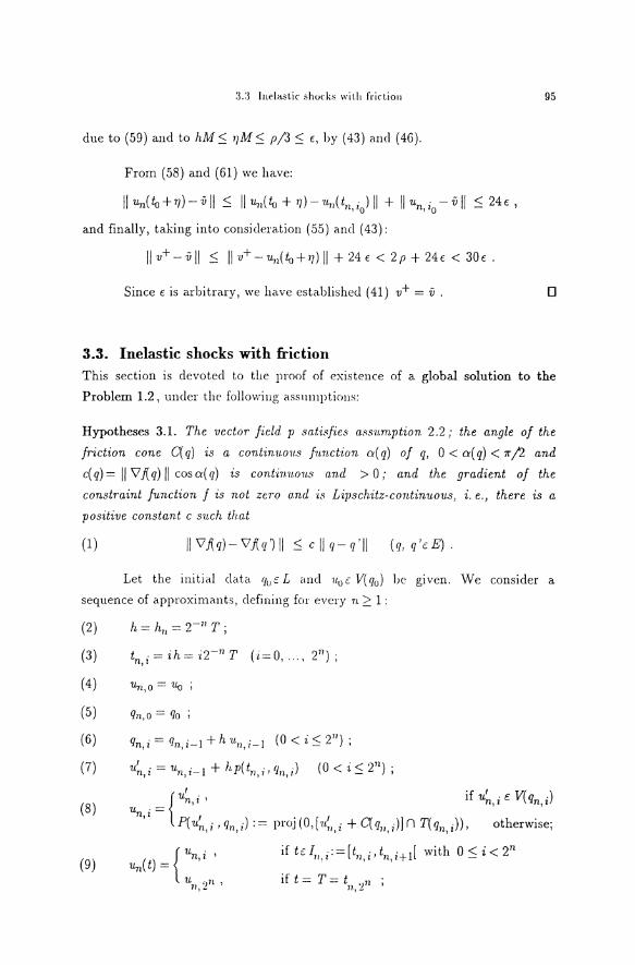
3.:3 lnelast.ic shucks witl. frictiou 95

due to (59) and to hM S 17M S p/3 S t, by ( 43) ancl ( 46).

From (58) and (61) we have:

II Un( lo + 1])- ii II S II Un( ~ + 17)- -nn(tn ; ) II + II un ; - ii II S 24 c ' , ·o ' o

and finally, taking into considera.tion (55) a.nd ( 43):

llv+-vll S llv+-un(io+17JII +24~: < 2p+24t: < 30~:.

Since Eis a.rbitra.ry, we have esta.blished (41) v+ = ii . 0

3.3. Inelastic shocks with friction This section is devoted to the proof of existence of a global solution to the

Problem 1.2, uncler the following assnmptions:

Hypotheses 3.1. The vector field p sa.tisfies a.ssum.ption 2.2; the angle of the

friction cone C( q) is a contin:twus fu.nction o( q) of q, 0 < o( q) < Jr /2 and

c( q) = II V 1{ q) II cos o( q) is continu.ou.s a.nd > 0; and the gradient of the

constraint function f is not zero a.nd ·is Lipsch:itz-continuov.s, i. e., there is a

positive constant c such tha.t

(1) IIVJ{q)-V.f{q'JII s cilq-q'll (q, q'EE).

Let the initial clata IJuf L and "lluf V(q0 ) be g1ven. We consider a

sequence of a.pproximants, defining for evcry n;::: 1 :

(2)

(3)

(4)

(5)

h = h" = 2-n T ;

t ·=ih=-i2-11 T (-i=0, ... ,211 ); n,z

Un,O = Uo ;

(6) qn,i = IJn,i-1 + h '11·n,i-J (0 < i S 2");

(7) u~,;=un,i-l+hp(t11 ,;,1Jn) (0<iS2 71 );

(8)

(9)

{ u~.; , if u~, i c: V( q11 )

un, i = P( 1t~ ; , q11 ;) : = proj (0, [·u.:, i + C( q" ;)] n T( qn ;)) , otherwise; l. '' ' 1 '

if lfl1~,;:=[tn,i•tn,i+l[ with 0 Si< 211

if t = T = t ·)n ; n,_

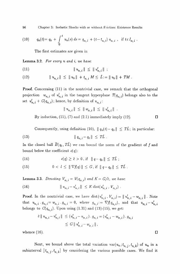
96 Chapter 3: Inelastic Shocks with or without Frietion: Existence Results

(10) q11(t)= q0 + jt U 11(s) ds = q11 ,; + (t- t",;) un,i , if tdn,i. 0

The first estimates a.re given in

Lemma 3.2. For every n and i, we have:

(11)

(12)

II un,; II ~ II ·u~. ;II

II uni II ~ II Uo II + tn j M ~ L:= II Uo II + TM· ' '

Proof. Concerning (11) in the nontrivial case, we remark that the orthogonal

projection w11 i of u;, i in the tangent hyperplane T( q11 ;) belongs also to the ' ' '

set u~ i + C( q11 ;) ; hence, by defini tion of 11.11 i: ' ' '

II un,i II ~ II w",; II ~ II ·u~,i II . By induction, (11), (7) and (2.1) immediately imply (12). D

Consequently, using clefinition ( 10 ), II q11(t)- q0 II < TL; in particular:

(13) II q11,;-qoll ~TL·

In the closed ball B( q0 , TL) we can bound the norm of the gradient of fand

bound below the coefficient c( q):

(14)

(15)

c(q) ;::: c > 0, if II q- q0 II ~ TL;

0 < l ~ IIY'.f(qJII ~ G,if llq-q0 ll ~TL.

Lemma 3.3. Denot-ing V11 ,; = V( q11 ) and K = G /c, we have:

(16) II u" ; - 11.;, ; II ~ K clist( u;, ; , v" ;) . ) ' l ., .,

Proof. In the nontrivial case, we have dist ( u;,, i ' vn, ;) = I Iu~. i - wn, i II . Note

that u11 i .g11 ;= W 11 i .g11 i = 0, where g11 ;:= 'Vj{q11 ;), and that u11 ;-u;, i ' J l l' ' ., ' '

belongs to C(q11 ,;)· Upon using (1.31) and (13)-(15), we get:

~ ( 1L;, i - ·u" i J · 9" i = ( u;, i - wn i ) · 9n i '- 1' ) . ' l '

~ Gllu;,,;-w",;ll,

whence (16). D

Next, we bound above the total variation var( u11 ;tn, j, t11 , k) of 1tn in a

subinterval ] t11 J., t11 k] by considering the various possible cases. We find it ' '

3.3 Inel~st.ic shocks wit.J, frict.ion 97

convenient to say tha.t if ·u.11 ,; = ·u.',,,; thc corrcsponding step ( at the instaut

t . ) is of free type; otherwise, it is a stql of contact type. n,'

Case #1. In the interval J = ]t11 1-, t k] there are only steps of free type. ' n,

Then llun,i-un,i-111 = llhp(t11,;,rzn)11:::; hManclaclclingupfromj+1 tok:

(17)

Case #2. In J only the last step is of contact type.

Then llun,k-l-un,jll:::; var(1t.71 ;t11 ,j,tn,k-l):::; M(tn,k-l-tn,j) (as m (17))

and, by construction, II u.',, k- ·u.11 k-l II :::; hM; whencc ' ,

Using (16) we have:

llun,k-u~,k11:::; Kclist(u',,,k, V11 ,k):::; K[dist(un,j• V11 ,k)+M(t11 ,k-tn)J

and we easily obtain the fonnula:

Case #3. In] only the endpoints a.re of contn.ct type.

Then in (18) we are able to control the clistance from u11 , j to V71 , k ( any

k > j):

(19) -·)

clist(1tn,j• vn,d:::; cy (tll,k-tll,j).

In fact, m the nontrivia.l case, ·u.n,j .!J11 ,k > 0 and, of course, un,j. 9n,j=O,

since u11 , j is a velocity after a. "contact". Elementary ca.lcula.tion shows that:

d' ( ·V )-(1ln,j·!l",A;)<l[- · - ·))<t_ll - ·II ISt un,J' n,k - II 9n,k II - l ull,J .(gn,k !ln,J - I 9n,k 9n,J '

by (12) and (15). On the other hancl (1), (10) ancl (12) imply that:

ll9n,k-9n,jll:::; cllrzn,k-q71 ,jll:::; cL(t11 ,k-tn,) ·

Thus, (19) follows and in this case we may replace ( 18) by the more precise:

(20) var ( U.n; t 71 1- , t11 k ) :::; R ( t71 k- t71 1 ) , ' , J '1

with R := M(1 +K) + KcL2jl (no rela.tion to the rca.ction measure dR).

Lemma 3.4. In the general case, the follo·wing estirnate holds:

(21)

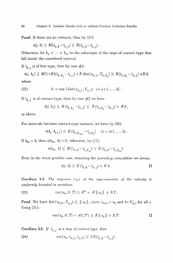
98 Chapter 3: lnelastic Shocks with or without Friction: Existence Results

Proof. If there are no contacts, then by (17)

Otherwise, let k1 < ... < km be the subscripts of the steps of contact type that

fall inside the considered interval.

If tn, j is of free type, then by case #2:

v(j, k1) ~ M(l+K)(tn k -t11 J·J+Kdist(1tn J.' Vn k) S R(tn k -tn J·) +Kd, ' 1 ' ' ' 1 ' 1 '

where

(22) d:=sup {dist(-u.11 1-, V11 ;): i=j+l, ... , k}. ' '

If tn, j is of contact type, then by case #3 we have

v(j, k1) ~ R ( t11 , k 1 - t11 ,j) S R ( t11 , kl- t11 , j) + K d ,

as above.

For intervals between contact-type instants, we have by (20):

v(k;, ki+l) S R(t11 k+ 1 -t11 ~,;) {i=j+l, ... , k). ' l l t

If km= k, then v(km, k) = 0; othenvise, by (17):

v(km, k) S M (t11 k- t" k ) S R (t11 k- tn k ) · 1 1 ru ' , nt

Even in the worst possible case, summing the preceding inequalities we obtain

0

Corollary 3.5. The seq·u.~Cnce ('u.71 ) of the a.pprox·imants of the velocity is

uniformly bounded in va.ria.tion:

(23) var(v.71 ;0, T) S K*:= Kll11v II + R T.

Proof. Wehave dist(ull,OJ vn,il s 111/v II, since 11-n,o = 1lv and Oe: vn,i for all i.

Using(21):

var{11-11 ;0, T) = v(0,211 ) S Kll 'llv II + R T. 0

Corollary 3.6. If t11 , j is a. step of contact tyzJe, then

(24)

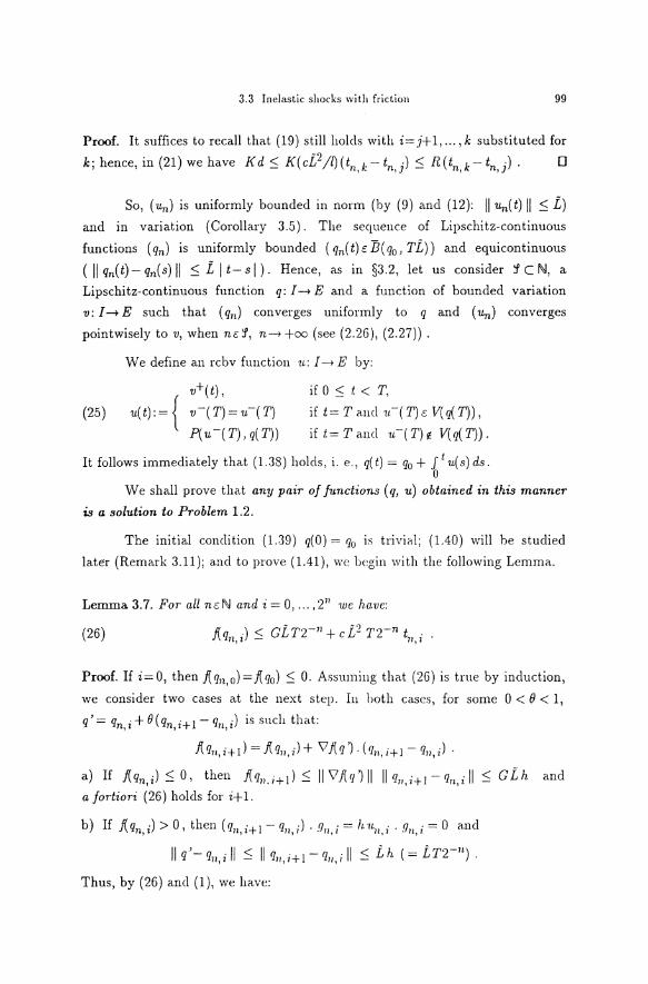
3.3 Inelastic shorks wit.h friction 99

Proof. It suffices to recall that (19) still holds with i= j+ 1, ... , k substituted for

k; hence, in (21) we have Kd S: K(cL2/0(tn,k-tn,j) S: R(tn,k-tn). D

So, ( u11 ) is uniformly bounded in norm (by (9) and (12): II Urr( t) II S: L)

and in variation (Corollary 3.5). The sequence of Lipschitz-continuous

functions ( q11 ) is uniformly bounded ( q11( t) E: B( q0 1 TL)) and equicontinuous

(llq11(t)-q11(s)ll S:Lit-sl). Hence, as in §3.2, let us consider jcN, a

Lipschitz-continuous function q: I-> E and a function of bounded variation

v: I-> E such that ( q11 ) converges uniformly to q and ( Un) converges

pointwisely to v, when nE f, n-> +co (see (2.26), (2.27)) .

(25)

We define an rcbv function 11.: I->E by:

v+( t),

u(t):={ v-(T)=u-(T)

P( u -( T), q( T))

if 0 S: t < T,

if t= T ancl n-( T) t: V( q( T)),

ift=Tand .,.-(T)~ V(q(T)).

It follows immediately that (1.38) holds, i. e., q(t) = q0 + J1u(s)ds. 0

Weshall prove that any pair of functions (q1 u) obtained in this manner

is a solution to Problem 1.2.

The initial condition (1.39) q(O) = q0 is trivial; (1.40) will be studied

later (Remark 3.11); and to prove (1.41), we bcgin with the following Lemma.

Le=a 3.7. For all nt:N and i = 0, ... , 2n we ha:ue;

(26) f\q ·) < GLTT 11 +cL2 TT 11 t . n,z - 11.,1

Proof. If i= 0, then 1\ IJn,o) = 1\ q0 ) S: 0. Assmning that (26) is true by induction,

we consider two cases at the next step. In both cases, for some 0 < B < 1,

1] 1 = 1]11 ;+B(q11 i+l- q11 ;) is such that: , , ,

fiqn i+l) = f{q" ;) + \7j{q') · (q" i+l- fJ11 .;) • ' , - ., ' '

a) H fiqn) S: o, then .f{q"·i+Il s: II \7./(q') II II rJn,i+I- rJ",; II s: GLh and a fortiori (26) holds for i+l.

b) If J\ IJn, ;) > 0, then ( q11 , i+ 1 - fJ11 , i) . .'J11 , i = h n11 , i . .'ln, i = 0 ancl

II I II < II II _< Lh (= LT2-1t). q- rJn,i - rJn,i+l-lfn,i

Thus, by (26) ancl (1 ), we have:

100 Chapter 3: lnelastic Shocks with or without Friction: Existence Results

j{qn,i+l) =J{qn)+ (Vj{q')-gn)·(qn,i+l-qn)

:; [ GLTT11 + c L2 TT 11 tn, ;] + ( cLh) L TT 11

= GLT2-n+ cL2 TTn t . n,1+l

Corollary 3.8. For all t EI, we h.ave .1{ q( t)) :; 0 ; th.at ·is:

(1.41) q(t)E L (tc: I) .

Proof. If t belongs to the set

(27) r . - { t1l' i : n ;::: 1 , 0 ::: i ::: 211 } '

D

then t is one of the nodes tm, j for ev<'ry sufficiently large m in f (in view of

our choice of the partitions ). The prececling Lemma implies that:

fiqm(t)) =fiqm):; T 111 ( GLT+cL2 T2 ).

Passing to the limit as m-. +oo, we obtain j{ q( t)) :; 0 for all tc r. Since r is

a dense subset of I and j{ q(.)) is a continuons function, the result follows. D

Hence (1.42), i.e., u(t)o:V(q(t)) holcls for o:::t< T. For t=T it IS

simply a consequence of definition (25 ).

Next, we prove two Lemmas.

Lemma 3.9. For every fixed XE E, the real function q -t dist(x, V(q)) is upper

semicontinuous.

Proof. Let dv = dist ( x, V( q0 )) and E > 0. The open ba.ll centered at x with

radius lfv + € intersects the convex cone V( q0 ). Since q-t V( q) is a lower

semicontinuous multifunctiou (Lemma 2.1 ), we have, for every q in some

neighbourhood of q0 , B( x, dv + E) n V( q) f= 0 , whence dist ( x, V( q)) < lfv+c. D

Lemma 3.10. Let 0 < t < T a.nd u-( t) E V( q( t)) .

(a) If € > 0, then there exist b > 0 und '~~DEN such tha.t

(28)

( b) The functions u and v are both continuous at t: u( t) = u-( t) = v( t) .

3.3 Inelast.ic shocks wit.h friction 101

Proof. ( a) Let us clenote 1t- = u.-(t) ancl V= V( q( t)). By the prececling Lemma,

we consicler a positive mtmber r such that, whenever II q- q(t) II :::; r,

clist(u- 1 V(q)):::; dist(u- 1 V)+~=~.

Next, we take b'c:]O,t:/2[ such that sc:I(b 1):=[t-D 1 , t+D 1 ] implies that

II q( s)- q( t) II :::; r /2. Moreover, by uniform convergence qn--+ q , we choose no insuchawaythat llqn(s)-q(s)ll:::; r/2 anclso

II qn ( s) - q( t) II :S r ( n ~ n0 ; n c: '.f ; s c:I( b 1 )) •

Picking, if necessary, a smaller b' and a !arger no, we may assume that t- b 1

and t + b ( 0 < b :::; b 1 ) are nocles of the consiclerecl approximants and that they

satisfy:

llv(t-b 1)-u-ll < ~ and ll·n11(t-b 1 )-v(t-D 1 )11 < ~ .

If t-D 1= tn,j ancl t+b= tn,k• we see that ll·un,j -1t-ll < c/2 ancl that, for

every i from j+ 1 to k,

clist(u11,j 1 Vn,;):S llun,j-·u-11 + clist(1t-, V(q 11 ,;)):::; t:.

Applying (21 ), we finally get :

var(un;t-D 1 t+b):::; var(u11 ;t-D 1 , t+b):::; Kt:+R(2b 1):S (K+R)t:.

(b) In particular, (28) implies that II ·u11 (t + b)- lln( t- b) II :::; (K + R) c, for every

!arge enough n c: '.f. Thus,

(29) II v(t+ o)- u(t- 8) II :::; (K+R) t,

by pointwise convergence ·n11 -> ·u. Letting b-> 0 ancl remembering that c is

arbitrary, we find that v+(t) = v-(t), that is, u(t) = u-(t). But (28) also

implies that II v(t+b)-v(t) II :::; (K+R) c and we cleduce similarly that

v+(t)=v(t). 0

Remark 3.11. Taking t = 0 ancl ·u- = vü, the prececling argument JS easily

adaptecl anclleads to the result v+(o) = ·u(O) (= limu11(0)=~). So:

(1.40) u(O) = 11ü .

Last but not the least, we have to cleal with the implications (1.43),

(1.44) and (1.45)- (1.47). Again, we choose the "base" measure:

(30) dp : = 1 d·n 1 + dt .

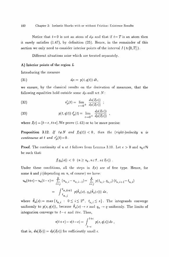
102 Chapter 3: Inelastic Shocks wit.h or without Fricli<m: Exist.cnce Results

Notice that i= 0 is not an atom of dp and that if i= T is an atom then

it surely satisfies (1.4 7), by definition (25 ). Hence, in the remainder of this

section we only need to consider interior points of the interval I ( tc-]0, T[).

Different situations arise which are treated separately.

A) Interior points of the rcgion L

lntroducing the measure

(31) dp:= p(t,q(t)) dt,

we ensure, by the classical results on the derivation of measures, that the

following equalities hold outside some dp-null set N:

(32) 1 ( ) _ 1. du.(/(t)) . 11.,, t - llll -1 ( '( )) '

f~u+ (P. 11 f

.J - . dp(!(t)) p(t, q(t)) &1,(t)- lun d (li( )) ,

f ....... o+ -fl E (33)

where I( E) = [ t- E, t+t ]. W e prove ( 1.43) or to be more precise:

Proposition 3.12. If t~ N and j{q(t)) < 0, th.en the (right-)velocity u zs

continuous at t and r'Jl( t) = 0.

Proof. The continuity of u at t follows from Lemma 3.10. Let E > 0 and 1lo c N

be such that:

f{ q" ( s)) < 0 ( n 2': nv , n E 1 , s d( E)) .

Under these conditions, all the steps in I(t) are of free type. Hence, for

some k and j ( depending on n, of course) we have: k k

'Un(l+t)-u"(t-t)= .L. (1Ln,i-'1111,i-l)= .L. p(tu,i•qu) (tn,i+l-tn,i) •=J •=J

Jt11k+l- -t '. p(B11(s), q11(Bn(s))) ds, n,J

where B"( s): = max { t", i : 0 :S ·i :S 211 , t11 , i :S s} . The integrands converge

uniformly to p(s,q(s)), because B11 (s)-> s ancl qn-> q uniformly. The limits of

integration converge to t- t and t+c Thus,

Jt+( v( t + E) - ·v( t - E) = p( s, q( s)) ds ,

1-f

that is, du(I(t)) = dp(I(t)) for sufficiently small t.

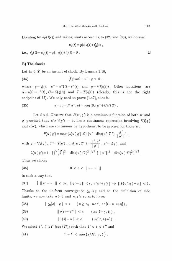
3.3 lnelastic shocks with friction

Dividing by dJ1(I(c)) and taking limits according to (32) and (33), we obtain:

u~( t) = p( t, q( t)) ~/ t) ,

1.e., r'll( t) = u~( t)- p( t, q( t)) t'Jl( t) = 0 .

B) The shocks

Let tc: ]0, 1[ be an instant of shock. By Lemma 3.10,

(34) .f(q)=O, u- .g > 0,

103

D

where q=q(t), u-=u-(t)=·v-(t) and g="V.f(q(t)). Other notations are

u=u(t)=v+(t), C= C(q(t)) ancl T=T(q(t)) (clearly, this is not the right

endpoint of I 1). We only neecl to prove (1.47), that is:

(35) u=z:= P(u-,q)=proj(O,(u-+C)n T).

Let S > 0. Observe that P( u ', q ') is a continuous function of both u' and

q' provided that u 'jO V( q ') - it has a continuous expression involving V!( q ')

and c( q '), which are continuous by hypothesis; to be precise, for those u ':

P(u',q')=max{,\(u',q'),O} [u'-dist(u', T') 11;;

11],

with g'="V.f(q'), T'= T(q'), dist(-u', T ')= ~>ll', c'=c(q') and

A(1L', q') = 1- [ (~~)2 -clist(-u', C')2 ]1/ 2 [ ll11 '11 2 -dist(-u', T')2 ]112 . c

Then we choose

(36) 0 < E < II u- 1L- II in such a way that

Thanks to the uniform convergence q11 -> q ancl to the definition of siele

limits, we now take ry > 0 ancl n0 E N so as to ha.ve:

(38)

(39)

( 40)

II qn( s)- q II < E ( n ?. no • n c f I s c [ t- 1] I t+ry]) '

llv(s)-11--ll < E

II v(s)-·ull < E

(sc:[t-1],t[),

(scjt 1 i+7J]).

We select t', t"c: r (see (27)) such tha.t t 1 < t < t" and

( 41) t "- t ' < mi n { E /MI TJ I S } .

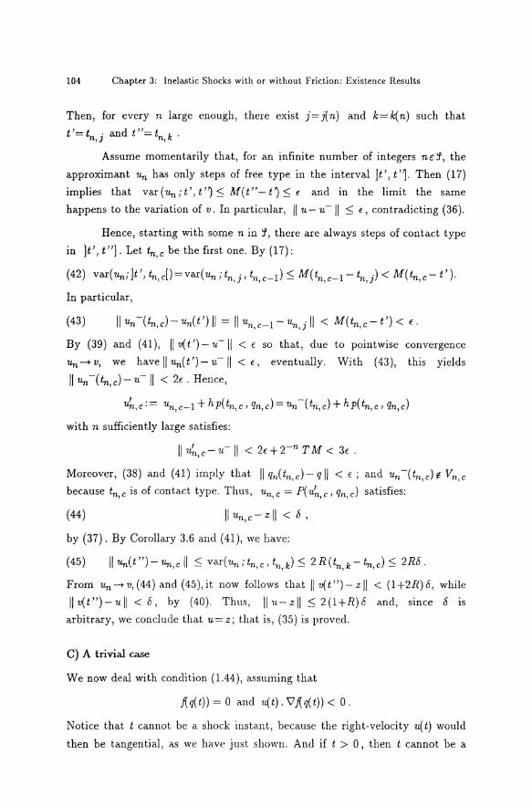
104 Chapter 3: Inelastic Shocks with or without Friction: Existence Results

Then, for every n I arge enough, there exist j = j( n) and k = k( n) such that

t'= tn 1. and t"= tn k . ' '

Assurne momentarily that, for an infinite number of integers nc: j, the

approximant Un has only steps of free type in the interval Jt ', t 'l Then (17)

implies that var(Un;t',t')-5: M(t"-t)-5: € andin the limit the same

happens to the variation of v. In particular, II u- u- II '5: €, contradicting (36).

Hence, starting with some n in j, there are always steps of contact type

m Jt', t"J. Let tn,c be the first one. By (17):

( 42) var( un; ]t ', tn, c[) = var( Un; tn, j, tn, c-l) '5: M( tn, c-1- tn, j) < M(tn, c- t' ).

In particular,

(43) llun-(tn,c)-un(t')ll = llun,c-1-un,jll < M(tn,c-t')< €.

By (39) and (41), II v(t')-u-11 < € so that, due to pointwise convergence

Un--+ v, we have II u11 ( t ')- u- II < €, eventually. With ( 43), this yields

II Un -(in, c)- u-11 < 2€ . Hence,

with n sufficiently large satisfies:

llu:1,c-1L-Ii < 2€+T11 TM< 3€.

Moreover, (38) and (41) imply that II q71(t11 ,c)-qll < €; and u11-(t11 ,c)~ Vn,c

because ln,c is of contact type. Thus, ·u11 ,c = P(u~,c, q11 ,c) satisfies:

(44)

by (37). By Corollary 3.6 and (41), we have:

(45) IIUn(t")-Un,cll '5: var(1L71 ;t11 ,c,tn,k)'5: 2R(tn,k-fn,c)'5: 2R5.

From u11 -+v,(44) ancl (45),it now follows that II v(t")-zll < (1+2R)5, while

llv(t")-ull <5, by (40). Thus, llu-zll '5,2(l+R)5 ancl, since 5 is

arbitrary, we conclude that u = z; that is, (35) is provecl.

C) A trivial case

We now deal with conclition (1.44), assuming t.hat

f{q(t)) = 0 ancl u(t). 'ilf{q(t)) < 0.

Notice that t cannot be a. shock instant, because the right-velocity u( t) would

then be tangential, as we have just shown. Ancl if t > 0, then t cannot be a

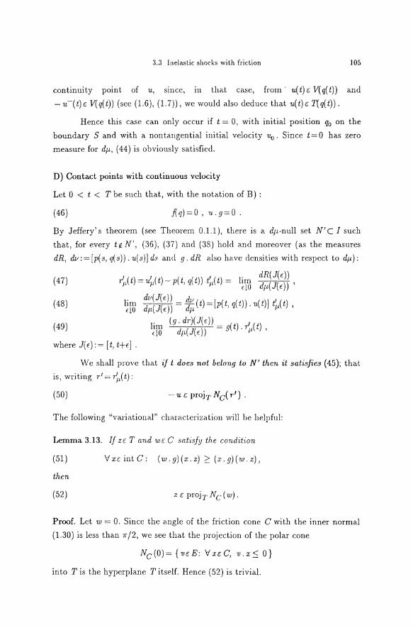
3.3 Inelastic shocks with friction 105

continuity point of u, since, in that case, from · u(t)c- V(q(t)) and

- u-(t)c- V(q(t)) (see (1.6), (1.7)), we would also deduce that u(t)c- T(q(t)).

Hence this case can only occur if t = 0, with initial position q0 on the

boundary S and with a nontangential initial velocity Uo. Since t= 0 has zero

measure for dfl, ( 44) is obviously satisfiecl.

D) Contact points with continuous velocity

Let 0 < t < T besuch that, with the notation of B):

( 46) fi q) = 0 ' 1/ .. g = 0 '

By Jeffery's theorem (see Theorem 0.1.1), there is a dft-null set N'c I such

that, for every t~ N', (36), (37) ancl (38) hold ancl moreover (as the measures

dR, du:= [p( s, q( s)) . u( s)] ds and g. dR also have densi ties wi th respect to df1):

( 47) 1 1 ~ . dR( J( E))

rp(t)=u11(t)-p(t, q(t)) ~Jl(t) = l;lJ dft(l(E)),

(48) du(](€)) du [ ] ,} l{pJ dp(J(E)) = dft (t) = p(t, q(t)). u(t) ~,lt)'

(49) 11.111 (g · dr)(J(E)) = (t) 1 (t) dO dp(J(E)) g . rJl '

where J(E):= [t, t+E].

Weshall prove that if t does not bclong to N' thcn it satisfies (45); that

is, writing r 1 = r'Jl( t):

(50)

The following "variational" characteriza.tion will be helpful:

Lemma 3.13. lf zc T and wc- C satisfv the condition

(51) Vxc int C: (w.g)(x.z) ~ (J:.g)(w.z),

then

(52)

Proof. Let 111 = 0. Since the angle of the friction cone C with the inner normal

(1.30) is less than 1r /2, we see that the projection of the polar cone

Ne (O) = { vc- E: V u c, v. x::::; o}

into T is the hyperplane T itself. Hence (52) is trivial.

106 Chapter 3: lnelastic Shocks with or without friction: Existence Results

Let instead wc:C, w -1-0. Then w.g< 0 ancl, choosing y:= z-::Z:9g, it is clear that z=projyy (since y-z is orthogonaltoT and zc: T). If x is any

interior point of C, then:

y.(x-w)=z.x-::Z:g(g.x)S: z.x-z.x=O,

using (51). By density, this is true for every xc:C. Hence yc:Nc(w) and (52)

follows. 0

Taken together with Lemma 3.13, the next Proposition establishes (50)

and ends the proof of the existence of a solution.

Proposition 3.14. We have:

(53)

(54)

r'c:C;

Proof. a) We prove (53). If 11 =0, it is trivial. If r' -1- 0 then, for every

sufficiently small E, dR(J(t)) -1-0 and dft(l(t)) > 0 (otherwise, (47) and the

convention 0/0 = 0 woulcl give r' = 0). Notice also that t has zero measure for

dp, ancl for dR. We must prove that (see (1.31)):

(55) r'. (- g) ~ c( q) II r' II . Let

(56) 0 < b < c( q)/2 .

Since the sequence of gradients \1 .!( q11 ( s)) converges uniformly to \1 .!( q( s)), which is a continuous function of s, then we may take some t > 0 and some 11o

for which II \7 .!( q11( s))- g II S: b for every s in J( E) and every n ~ 11o. In

particular, all the 9n, i : = \7 .!( q11 ( t")) corresponding to nodes falling inside

]t, t+t J , say those with i = j, ... , k , ·will satisfy

(57) (n ~ nv, nd') .

The coefficient c( q) is also a continuous function of q; so, by the same

argument, we can ensure that:

(58) II c( q")- c( q) II s: b .

By construction, either r 11 i: = ·u11 i- u~ i IS zero or it IS equal to I ") .,

P(u111 i,q11 j)-u~ic:[u~i+C(q11 i)J-u;1 i; hence, r -belongs to C(q11 i)· By

! I I J ., 1 n,'l. I

3.3 Inclastic shocks with frict.ion

definition of the friction cone (1.31) aml adding up from j to k, we obtain:

By (57) and (58), we deduce that

k k L: r71 ;-(-g)+8 L: i=j , i=j

i. e., with Pn i := p(t71 ;, qn ;): , , ,

107

(59) k k L: (un ;- un i-1- hp" ;) · (- g) 2': [c(q)-28] .I: II un,i- un,i-l- hpn,i 11-

i==j ' , , 1.;::::::.)

Let eil: I---> I and Pn: I---> E be defined by BH(O) = 0,

(60)

(61) p,b) := p(B,b),q,,(fJ"(s))) (= P",i, if s.sJtn,i-1,tn,iJ).

Then in (59) we have: k k L: T n i = L: ( u" i - 11·n i -1 - hp" i) i=j ' i=j ' ' 1

1n k = ·u." k-"1/." y-1 + j , Pn(s)ds , , t

n, j-1

!011(t+<) = n11 (t+c)- u. 11(t-E) + , p 71(s) ds.

011( t)

Let us take Iimits with respect to n. Since tn,j-1 ---> t, tn,k---> t+c,

since B11(s) converges uniformly tos ancl p"(s) converges uniformly to p(s, q(s)),

then we obtain in the Iimit:

Jt+c 1L(t+c)- u.-(t) + p(s, q(s)) ds;

t

here, we have used continuity of u a.t t (see Lemma. 3.10 (b)) a.nd also assumed

that u is continuous a.t t+t. Therefore: k

(62) !im L: r11 ;=(d1L- p(s, q(s)) ds) ([t, t+c])= dR(l(<)), 1 i=j ,

hence

(63)

Thanks to (56), ( 62) a.ncl ( 63 ), we infer from (59) that:

dR( J( E)) . (-g) 2': [ c( q) - 28] II dR( J( E)) II , for every small E such tha.t t+< is a. continuity point of u. Dividing by

108 Chapter 3: Inelastic Shocks with or without Friction: Existence Results

dJ.L( J( €)) > 0, letting € go to zero and using ( 4 7), we get:

r'.(-g) ~ [c(q)-28JIIr'll·

As 8--+ 0, this produces (55); that is, r' E C.

(b) In view of proving (54), we consider xcint C(q(t)): x.( -g) > c(q) II xll· If

s is near tot, then we also have x.(-'Vj{q(s))) > c(q(s)) llxll and, by

uniform convergence, this still holds for q11( s) , starting at some n. In other

words, for some 11tJ and c0 :

(64) (0 < € ~ € 0 ; n ~ 11tJ, nd')

provided that t11 ;E ]t, t+c] , which happens for, say, i = j, ... , k. ,

Webegin by establishing the discretized equivalent of (54), namely:

(65)

lf r 11 ;=0, then this is trivial. If not, then we are dealing with a step of contact , type. Thus u~ i. g11 i > 0 and u11 i = proj(O, ( u~ i + C11 ;) n T11 ;) where

' ' ' ' ' ' T11 ;=T(q11 ;)· Moreover, u11 ;-911 ;=0 and 9ni·x<0, by (64). So,

) ' ' ' ' 1

>.:= (r11 ;·9n ;)/(911 ;.x)= -(u;1 ;·9n ;)/(g71 ;-x) is positive and it is readily ' ' ' '' ' '

seen that z: = u~ i +).X belongs to ( u~ i + cn ;) n Tn i (indeed, z. 9n i = 0). ' ., l ' '

Since un,i is, by definition, the proximal point of 0 in this set, we have

u11 i. (z- u11 ;) 2 0, whence: , ,

(66)

Given the definition of >., if we multiply (66) by the negative number g11 ·. x, ,I

then we obtain (65).

Now, we consider any 8 > 0 a.nd obtain a 8-approximate version of (54)

(see (84) below). Recalling that u-(t)=11(t)c V(q(t)), by Lemma 3.10(a) we

choose € 0 > 0 and 11tJ E :f such tha.t

(67) var (1tn; t, t+t:) ~ 2ll8x II '

for every € ~ c0 and every n ~ 11tJ in :f. We can also guarantee that, as in (57):

(68)

and thanks to Lemma 3.10 (b) a.ucl to pointwise convergence ·u11 --+ v :

(69) ll·un(t) -1L II ~ 2 118x II .

3.3 Inelastic shocks with friction 109

From (64) and (68) we get

(70) 0 > 9n, i . X 2=: g . X - 5 .

On the other hand,

(71)

In fact, in the nontrivial case r11 , i # 0, observing that -g11 , i is an interior

point of C( q11), we have by (66):

un i · r n i ~ -), ( un i · 9n i) = 0 · l I -, l

Thanks to (70) and (71), the right-hand siele of (65) JS bounded above as

follows:

(72)

For i=j, ... ,k, from (67) we obtain that llun,i·x-un(t).xll ~ 5/2, while

llu11(t).x-u.xll ~ 5/2 (by (69)); so, u11,;.x~ u.x+5. Since 9n,i·rn,i~O

(rn,ic: cn,il' we have:

(73)

Now, we use (65), (72) and (73) and sum from j to k:

k k (74) (u. x+ 5) .L. g11 ,;. r11 ,; ~ (g. 1:-8) .L ·u.11 ,;. r",;.

!=) I=)

To obtain an upper bound of the right-hancl side of (74) we must give a lower

bound of the sum therein, because g. x- o < 0 (xc: C). With the use of 2.3(20), k k k

(75) .L. u", i · r", i = .L. un, i · (u"' i- ·u"• i-1) - .L. ( un, i · Pn, i) h l=J !=) •=J

t 1 2 1 . 2 J n, k+ 1 ,

2=: (2111tn(t+c) II -211u"(t) II ) - t . Pn(s). un(s) ds, n, J

where p11(s):=p(B11(s), q11(B 77 (s)))=p 71 ; (if sc:[t11 ;,t11 i+d); 077 is clefinecl in the , , , proof of Proposition 3.12.

Let n-> += ( n E f).

The first two terms lll the right-hancl siele of inequality (75) converge to

d(i II u 11 2) (l(t)), if t+t is assuuwcl to he a continuity point of 1L. Regarding the

integral, since llß71(s).1tn(s)ll ~ ML, t11 ,j->t, t11 ,k->t+t, un(s)->v(s) and

p11(s)-> p(s, q(s)), by applying thc clomiua.tecl convergence theorem we obtain

in the limit:

110 Chapter 3: Inelastic Shocks with or without Friction: Existence Results

Jt+f Jt+(

p( s, q( s)) . v( s) ds = p( s, q( s)) . u( s) d~ = dv( J( €)) . t I

Hence (75) implies k

(76) limsup [ (g. x- 8) L u11 i. r11 ;] :-:; (g. x -8) [ d(~ 111tll 2)- dv](J(E)). ":! i=j ' ' -

Turning now to the left-ha.ncl siele of (74), we see that:

(78) g11(s)-> g(s): = 'Vf( q(s)) uniformly on I.

Therefore:

(79) k k L 9n;·(uni-uni-l)= .L . .Iln(t",;).d·nn(Jtn,i-l•tn,i]) i=j , ) l 1=)

= j]t . 1 ] !]71 (s). du71(s)= j]t t+c] g11(s). du11(s). n,;-1' n,k '

By virtue of (67) ancl (78):

(80) 1 j [g11(s)- g(s)J. rlu."(s) I :-:; II !Jn-g II oo ~118 II _, o, ]I,IH] X

when n-> +oo, n remaining in :f. But, by Theorem 0.2.2(ii) [0.2(10)] ancl

recalling that g is a continuous function ancl that both u and v are continuous

at t and at t+c, we see that:

limj g(s).du11(s)=j g(s).dv(s)+g(t).[v+(t)-v(t)] ":! ]t, IH] ]t, l+f]

- g(t+c). [v+(t+E)- v(t+E)]

= j g(s). dn(s) . [I,IH]

If taken together with (79) ancl (80), this implies:

(81) k J lim L g" ;.(u" ;-u" i-tl= g(s).du(s). ":! i=j ' '. ' [t, IH]

The remairring term in (77) may be written in the form:

k k 1n k .L.(9n,i·Pn)h=.L. [gn(t",;).p"(t11 ,;)](t11 ,i-t11 ,i-l)= jt' 9n(s).p,b)ds, I=J z=J n,j-1

hence it can be shown to converge to f /+( g(s). p(s, q(s)) ds (use (78) and so

on). Combining with (77) and (81), it tmns out that:

(82) k J lim L 9n ;·rn ;= g(s).[du(s)-p(s,q(s))ds]=(g.dR)(J(E)). j i=j ' ' [t, l+i]

3.3 Inelastic shocks with friction 111

From (74), (76) and (82) it follows that:

(83) ( u. x + 8) (g. dR)( J( t)) :::; (g. x- 8) [ d(t II u 11 2)- dv ]( J( E)) .

Divide (83) by dJ1.(l(t)) and let t go to zero, always with u continuous at t+c. Thanks to (2.38) and ( 4 7)-( 49), this yielcls

( u. x + 8) (g( t) . r'l-'( t)) :::; (g. x- 8) {! [ u( t)+u-( t)] . u'l-'( t)- [p( t, q( t)) . u( t)] fl-'( t)}

= (g. x- 8) { 1t( t) . [ u~(t)- p( t, q( t)) fl-'( t)] } ,

that is, with the notation introcluced above:

(84) ( U. X+ 8) (g. r') :::; (g. X- 8) ( U. r') .

Letting 8-> 0 in (84), we obtain at last conclition (54):

(u.x)(g.11):::; (g.x)(u.r'). 0

Rcmark 3.15. The assumption 3.1 can be localizecl: if we only assume that the

gradient of J is locally Lipschitz-continuous (e.g. that f is c2) then the sarne

method provieles a local solution to Problem 1.2.

Rcmark 3.16. When it is rea.sonable to neglect the forces acting upon the

considered system, i. e., to take p = 0, tlten we only neecl to assume that f be

of class C1. The main difference is in the search for an upper bound of the total

variations of the velocity a.pproximants: we may proceed in another manner,

closer to the one adoptecl in §3.2.

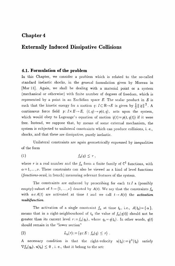
Chapter4

Externally lnduced Dissipative Collisions

4.1. Formulation of the problern In this Chapter, we consider a problern which is related to the so-called

standard inelastic shocks, in the general formulation given by Moreau in [Mor 11]. Again, we shall be dealing with a material point or a system

(mechanical or otherwise) with finite number of degrees of freedom, which is

represented by a point in an Eucliclian space E. The scalar product in E is

such that the kinetic energy for a motion q: I C IR->E is given by ! II q 11 2 . A

continuous force field p: I X E-> E, ( t, q)-> p( t, q), acts upon the system,

which would obey to Lagrange' s equation of motion 'q( t) = p( t, q( t)) if it were

free. Instead, we suppose that, by means of some external mechanism, the system is subjected to unilateral constraints which can produce collisions, i. e.,

shocks, and that these are clissipative, purely inelastic.

Unilateral constraints are again geometrically expressed by inequalities

of the form

(1)

where r is a real number and the fa form a. finite fa.mily of e1 functions, with

a = 1, ... , 11. These constraints can also be viewed as a kind of level functions

(fonctions-seuil, in french) mea.suring relevant features of the system.

The constraints are enforced by prescribing for each tc; I a (possibly

empty) subset of ~: = {1, ... , 11} denotecl hy A( t). We say that the constraints fa with a c; A( t) are activated at time t and we call t-> A( t) the activation mv.ltifv.nction.

The activation of a single constraint fa a.t time to, i.e., A( to) = { a },

means that in a right-neighbourhood of t0 the value of fa( q( t)) should not be

greater than its current level r: = fa( q0 ), where q0 = q( to). In other words, q( t) should remain in the "lower section"

(2) La( r): = { qc: E: fa( q) :::; r} .

A necessary condition is that the right-velocity u( to): = q_+( to) satisfy

'V fa( q0 ) • u( to) :::; 0 , i. e., that i t belong to the set:

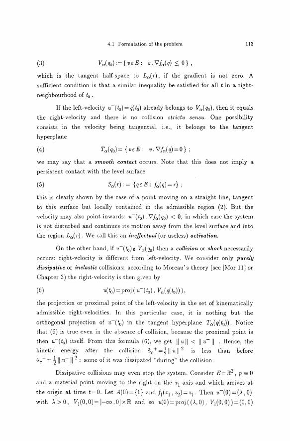
4.1 formulation of the problem 113

which 1s the tangent half-space to La( r), if the gradient IS not zero. A

sufficient condition is that a similar inequality be satisfied for all t in a right­

neighbourhood of fo.

If the left-velocity u-( fo) = q( fo) already belongs to Va( q0 ), then it equals

the right-velocity and there is no collision strictu sensu. One possibility

consists in the velocity being tangential, i.e., it belongs to the tangent

hyperplane

(4)

we may say that a smooth contact occurs. Note that this does not imply a

persistent contact with the Ievel surface

(5) Sa(r):= {qcE: fa(q)=r};

this is clearly shown by the case of a point moving on a straight line, tangent

to this surface but locally conta.inecl in the a.clmissible region (2). But the

velocity may also point inwarcls: 1L-(fo). 'Vfa(q0 ) < 0, in which case the system

is not disturbecl ancl continues its motion awa.y from the level surface and into

the region La(r). We call this an ineffectual (or useless) activation.

On the other hancl, if 1L-(t0 ) ~ V('(( q0 ) then a collision or shock necessarily

occurs: right-velocity is different from left-velocity. We cousider only purely

dissipative or inclastic collisions; a.ccording to Moreau' s theory ( see [Mor 11] or

Chapter 3) the right-velocity is then given by

(6)

the projection or proximal point of the left-velocity in the set of kinematically

a.dmissible right-velocities. In this pa.rticular case, it is nothing but the

orthogonal projection of u-(lo) in the tangent hyperplane Ta(q(fo)). Notice

that (6) is true even in the absence of collision, because the proximal point is

then u-(fo) itself. From this formula (G), we get ll·u II < II u-11 . Hence, the

kinetic energy after the collision ~c + = ~ 1111.11 2 IS less tha.n before

~c- = ~ II u-11 2 : some of it was clissipated "du;.ing" the collision.

Dissipative collisions ma.y even stop the system. Consider E= IR2 , p = 0

and a material point moving to the right on the x1-axis and which arrives at

the origin at time t= 0. Let A(O) = {1} a.ncl h (x1, x'2) = x1. Then u-(0) = (-\, 0)

with -\>0, V1(0,0)=]-=,0]x1R ancl so 1L(0)=proj((,\,O), V1(0,0))=(0,0)

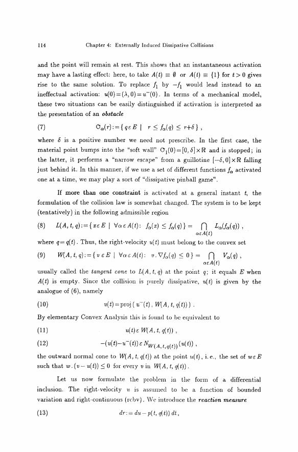
114 Chapter 4: Externally lnduccd Dissipative Collisions

and the point will remain at rest. This shows that an instantaueaus activation

may have a Iasting effect: here, to take A( t) = 0 or A( t) = {1} for t > 0 gives

rise to the same solution. To replace j 1 by -h would Iead instead to an

ineffectual activation: u(O) = (>., 0) = u-(0). In terms of a mechanical model,

these two situations can be easily distinguished if activation is interpreted as

the presentation of an obstacle

(7)

where 8 is a positive number we neecl not prescribe. In the first case, the

material point bumps into the "soft wall" 0 1 (0) = [0, 8] x IR and is stopped; in

the latter, it performs a "narrow escape" from a guillotine [ -8, 0] x IR falling

just behind it. In this manner, if we use a set of different functions fa activated

one at a time, we may play a sort of "dissipative pinba.ll game".

lf more than one constraint is activated at a general instaut t, the

formulation of the collision law is somewhat changed. The system is to be kept

(tentatively) in the following admissible region

(8) L(A,t,q):={xcE/ Vac:A(t): fa(x):S:fa(rz)}= n La(f0 (q)), a<A(t)

where q= q(t). Thus, the right-velocity u(t) must belang to the convex set

(9) W(A,t,q):={vc:E I Vac:A(t): v.\lfa(q):::: 0} = n Va(q)' a<A(t)

usually called the tangent cone to L( A, t, q) at the point q; it equals E when

A( t) is empty. Since the collision is purely clissipative, u( t) is given by the

analogue of (6), namely

(10) u( t) = proj ( u-(t), W(A, t, rz( t))) .

By elementary Convex Ana.lysis this is founcl to be equiva.lent to

(11)

(12)

u(t)c: W(A, t, rz(t)),

-(u(t)-u-(t))c: NW(A,t,q(t)) (u(t)),

the outward normal cone to W(A, t, q(t)) at the point u(t), i.e., the set of wc:E

such that w. ( v- u( t)):::; 0 for every v in W(A, t, q( t)).

Let us now formulate the problern in the form of a differential

inclusion. The right-velocity 11. is assumed to be a function of bounded

variation and right-continuous (rcbv). \Ve introduce the rcaction measure

(13) dr:= du- p(t, rz(t)) dt,

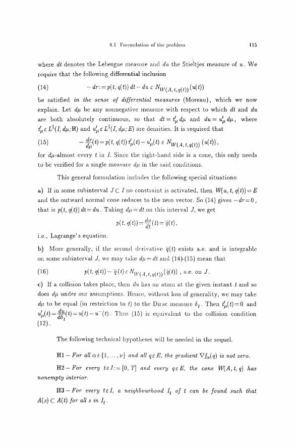
4.1 Fonnulation of the problem 115

where dt denotes the Lebesgue measure a.nd du. the Stieltjes measure of u. We

require that the following differential inclusion

(14) - dr: = p( l1 q( t)) dt- dn c: NW(A, t, q( t)) ( u( t))

be satisfied m the sense of difjeTential meas·ures (Moreau), which we now

explain. Let dfl- be any nonnegative measure with respect to which dt and du

are both absolutely continuous, so that dt = t!Jl dfl- and d·u = u~ dfl-, where

t!Jl c. L1(I1 dfl-;IR) and u.~ c. L1(I1 df1-; E) are densities. It is required that

(15) - ~~(t)=p(t1 q(t))f,,(t)-v.~,(t) c. NW(A,t,q(t)) (u(t)),

for dfl--a.lmost every t in I. Since the right-hand siele is a cone, this only needs

to be verified for a single measure dp in the said conditions.

This general formulation inclucles the following special situations:

a) If in some subinterval J C I no constraint is activated, then W( a1 t1 q( t)) = E

and the outward normal cone recluces to the zero vector. So (14) gives -dr= 0 1

that is p( t1 q( t)) dt =du. Taking d11 = dt on this interval J, we get

p( t, q( t)) = ~~; ( t) = '<j( t)'

1.e., Lagrange' s equation.

b) More generally, if the second derivative 'lj(t) exists a.e. and is integrable

on some subinterval J, wc may take dit=dt a.ncl (14)-(15) mean that

(16) p(t, q(t))- 'tj(t)c: NW(A,t,q(t))(iJ(t)), a.e. on J.

c) If a collision takes place, theu du. has au atom at the givcn instaut t and so

does dJ.L under our assumptions. Hcncc, without loss of generality, we may take

dp to be equal (in restriction to t) to the Dirac measure 51 . Then f,,( t) = 0 and

u;,(t)=j;(t)=u(t)-u-(t). Thus (15) is equivalent to the collision condition

(12). t

The following technical hypotlwses will he needecl in the sequel.

H1 - For all a c.{ 11 ... , v} and a.ll q t. E, th.e gmdient 'V fn:( q) is not zero.

H2- For every tc: I:= [0 1 T] and every qt. E, the cone W(A, l1 q) has

nonempty interior.

H3- For every t c. I, a neighbourhood I1 of t can be found such that

A(s) C A(t) for all s in I1 .

116 Chapt.er 4: Extcmally Induced Dissipative Collisions

H4- The force field p is continuous and bounded:

(17) II p( t, q) II ~ M (tel, qc. E).

H5- The force field is L-ipschitz-cont·inuous with respect to q and there

exists a positive constant k such that:

(18) II p(t, q)- p(t, q') II ~ k II q- q'/1 (tef, qE E) .

Comments. Hypothesis H1 ensures that the level surfaces are really

(hyper)surfaces, which are the topological boundaries of the respective sets

L( a, r), and that the unit outer normal is given by

Hypothesis H2 is a version of the usual cone condition on the regularity of the

boundary and is needecl for instance to .avoicl sharp corners. In Mechanics, this

type of requirement is sometimes callecl a "safe load" condition.

Hypothesis H3 tells us that immecliately before or after any given instant t we

may not activate more constraints tha.n at t. Mathematically, this can be

expressed by saying that the activation multifunction A IS upper

semicontinuous from I (with its usual topology} to {1, ... , v} (with the discrete

topology). This is not a stringent restriction on A. lncleed, it allows the

treatment of more general motions than the classical "finite-type" ones, where

A is piecewise constant; for instance, the accumulation of collision instants is

admissible.

Hypotheses H4 and H5 yield existence ancl uniqueness of solution to Lagrange' s equation. They could possibly be weakened, but that is not the

essential aim of this study.

Also, we could require these hypotheses to be satisfied only for all q in some

neighbourhood of the given initial position q0 ; the following main existence

theorem would then be replaced by a. local existence result.

Theorem 1.1. Assurne H1-H5. Let q0 c. E and an admissible initial velocity

TJ.oE W(A, 0, q0) be given. Then, there exists a Lipschitz-continuous function

q: I-+ E with q(O) = q0 and such that

(19) q(t)=q0 + jt 1t(s)ds 0

(tc. I:=[O, T]),

4.2 Existence of a solution 117

where u: I____, E (the right-velocity) is a. r·ight-contimwus f<mct·ion of bounded

va.ria.tion and sa.tisfies:

(20) u(O)=q+(O)=~

(21) u(t)c W(A, t, q(t)) (tc[);

(22) p(t, q(t)) dt- duc NW(A,t,q(t)) (·u(t)),

in the sense of differential mea.sures expla.ined above.

The proof is given in §4.2 ancl it relies on Schauder' s fixecl point

theorem and on the existence results for lower semicontinuous sweeping

processes of Chapter 2. In §4.3 we discuss the rclation of this problem with the

problem of inelastic shocks alle! also the questions of uniqueness and

clepenclence on the data.

4.2. E:ristence of a solution Let us take A ancl f 01 (o: = l, ... , r;) satisfying tl1e assumptions of Theorem 1.1.

To simplify the notation, we shall omit A in expressions such as W(A, t, q).

Lemma 2.1. ( a.) The rn:nltifu.nction ( t, q) __, W( t, q) ·is lower semicontinuous m

IxE.

( b) If t ____, q( t) is a. continuO'ItS function from I to E, thcn

(1) t____, W(t, q(t))

zs a l. s. c. multifnnction ·in I ·with closed convex va.Z.nes ha.ving nonempty

interior in E.

Proof. (a) Let U be an open subset of E suchthat

(2) un W(t,q) -10.

Hypothesis H2 says that the closed convex set W( t, q) ha.s nonempty interior;

hence, it is equa.l to the closure of its interior. Then (2) implies tha.t U also

intersects int W(t, q). Let Vc u n int W(t, q). By clefinition (1.9) ancl

hypothesis Hl, this implies tha.t

·v. 'Vf01 (q) < 0 (ocA(t)).

118 Chapter 4: Externally Induced Dissipative Collisions

As all the given functions fo: are e1, there exists a neighbourhood U q of

q in E, such that for every y c: Uq :

(3) v. \lfcr(Y) < 0 (ac:A(t)).

By H3, we can choose 11 , a neighbourhoocl of t in I such that

(4) A(s) C A(t) (sdt) .

Then, condition (3) is satisfied for every s in !1 and every a c: A( s) C A( t). Thus, vc: W(s, y) and

(5) W(s,y)n U:j:.0

which proves that W(.,.) is lower semicontinuous in Ix E .

(b) It follows immediately from (a), beca.use the composition of a continuous

function with a lower semicontinuous multifunction gives a lower

semicontinuous multifunction. 0

We now begin to construct a. fixed point scheme inspired by some

remarks by Moreau ([Mor 11], end of §8).

Consider the set

K:={q:J__.E/ q(O)=q0 , llq(t)-q(s)II:SR/t-s/ (t,sd)},

where R: = II Uo II + TM is an a priori bouncl for the right-velocity, as shown

below. It is clear tha.t K is a. convcx set of a.bsolutely (more precisely,

Lipschitz) continuous functions. Since K is by definition equicontinuous,

uniformly bounded ( II q II 00 :S II q0 II + R T) a.nd closed, then by Ascoli­

Arzela' s theorem K is compa.ct in the Banach space of continuous functions

C(I, E) with the uniform convergence norm. The set K may be presented in

another way. Let the prim.itivation opera.tor P: ux'(I, dt; E) __. C(I, E) be

defined by

(6)

We have:

(7)

Pu( t) = q0 + j t u( s) ds .

0

K = {Pu I uc: L=, //u II 00 :S R} .

To every function qE K we associate the multifunction

(8) t

t__.fq(t):= W(t,q(t))- j p(s,q(s))ds. 0

4. 2 Existence of a solu tion 119

By virtue of Lemma 2.1(b) and continuity of the integral term, rq is a lower

semicontinuous multifunction with closed convex values having nonempty

interior. Moreover, ~c: W(O, q0 )=rq(O). Hence the results of Chapter 2, §4

ensure the existence of a unique rcbv function Vq: I--+ E such that

(9)

(10)

(11)

vq(O) = <to ;

vq(t)tTq(t) (tc: I);

- dvq c: Nr q(t) ( vq( t)) ,

in the sense of differential measures. Let us write

It is equivalent to say that the function

(12) uq(t):=vq(t)+ j 1p(s,q(s))ds 0

(td),

satisfies the following three conclitions:

(13)

(14)

(15)

uq(O) = ·u1J

1tq(t)c: W(t, q(t)) (td);

p(t, q(t))dt- dnq c NW(t,q(t))(uq(t)),

again m the sense of Moreatl. In fact, (15) is casily shown, by taking

dp = I dvq I + I duq I + dt and obscrving tha.t duq = p( t, q( t)) dt + dvq and

Nr(v)=Nr+x(v+x), for every x in E and every convex set r.

We now establish 1111 a priori bouncl on the solution to (13)-(15):

(16) II uq( t) II S: R : = II v1J II + TM ·

We denote by ~~ and u~,p the densities of dt and duq with respect to dp. Then,

by (15), we have, for dp-almost every t:

p(t, q(t)) t;Jt)- n~1 , 1 ,(t):: NW(t,q(t)) (uq(t)) .

Since W( t, q( t)) is a convex cone, this gives elementarily:

[p(t,q(t))~,(t)-1t~1,Jl(t)].nq(t)=O,

i.e., uq(t).p(t,q(t))t'p(t)=uq(t).1t~,p(t), dp-almost everywhere. Multiplying by

dp, we obtain the following equality of realmeasures:

(17) 1/.IJ • p( . ' q( . ) ) dt = "U.q • d<tq .

120 Chapter 4: Extemally lnduced Dissipative Collisions

Moreover, the inequality

(18)

holds at the continui ty points of uq ( trivially) . It also holds at any point of

discontinuity, because then ( 15) implies that <tq( t) = proj ( uq -(t), W( t, q( t))) and

we know that the projection is nonexpansive and 0 belongs to the set into

which the projection is macle. Proceecling as in [Mor 11] (8.11)-(8.15), it follows

from (17), (18) ancl H4 that the rcbv function 1/>(t):= II u9(t) II satisfies:

r d4 ~ ~d(l/>2 ) = ~d(uq. uq) ~ Uq. duq ~ 1/>Mdt ~ r Mdt;

whence d4 ~ M dt, in any snbinterval wlwre 1/J- is never zero. More precisely

and without any restriction, we ran decluce, as suggested by the last

inequality, that 1/>(t) ~ 1/>(0)+Mt, i.e.,

ll·uq(t) II ~ ll·1ftl II +Mt

ancl (16) follows.

Fix R' > R. It follows from (12), (14) ancl (16) that vq(t) belongs to the

set

(19) Cq( t) : = [ W( t, q( t)) n B ( 0, R ') ]- j 1 p( s, q( s)) ds , 0

so that, applying the next Lemma, we see that vq is also the solution to the

sweeping process by Cq .

Lemma 2.2. Let C C E be a. closed cm1·uex set a.nd XE. C. If II x II < R ', then

(20)

Proof. If VE. Ne( x), that is, if v. ( y- x) ::; 0 for all yE. C, then the same is true

for every y in the set c ': = cn B(O, R ') 'hence VE. Ne .(x).

Conversely, assume that v.(z-x) ~ 0 for every zcC' and consider an

arbitrary y in C. If fh]0,1[ is sufficiently small, then z8 :=x+B(y-x) still

belongs to the convex set C. Moreover II z0 II < R ', because z8 ---> x when

8---> 0. Thus z8 c C' ancl by hypothesis ·u. (z0 - x) = B v. (y- x) ~ 0 . Since

B>O,wehave v.(y-x) ~ 0 anclso vENC,(x). 0

We prove that the opcrator 0': q---t vq is strongly continuous from K into

Loo.

4.2 Existence of a solution 121

Consider a sequence of functions ( q11 ) C K that converges uniformly to

q€ K. Concerning Hausdorff distances, it will be shown later that

(21) h11(t):=h(W(t,q11(t))nB', W(t,q(t))nB')-->0 uniformlyinJ,

where B'= B(O, R '). Then a simple calculation and H5 yield

h(Cq11(t),Cq(t))~ h11(t)+ II j 1 p(s,q11(s))ds- j 1 p(s,q(s))ds II 0 0

~ h11(t)+ jt kllq11(s)-q(s)ll ds 0

~ h11( t) + k T II q"- q II oo

so, the Hausdorff distances h ( Cq 11( t), Cq( t)) converge uniformly to zero.

Furthermore, since the intersection of I. s. c. multifunctions is still I. s. c. ( see

[Ber], Ch. VI, § 2) both Cq 11 ancl Cq are lower semicontinuous multifunctions

taking closecl convex values with nonempty interior. Then, by Corollary 2.4.14,

the solutions to the respective sweeping processes with initial value ~ satisfy

Vq 11 ( t)--> vq( t) uniformly on I.

The (Picard type) integral operator 'J: K--> L 00 defined by

(22) 'J(q)(t):= j 1p(s,q(s))ds (qcK,tci), 0

is also strongly continuov.s. In fact, by H5:

thus

(23)

II <J(q)(t)-'I(iJ)(t) II ~ k j 1 llq(sJ-iJ(slll ds ~ kTIIq-t1lloo 0

II <J( q)- <J( iJ) II oo ~ k T II q- iJ II oo .

Therefore, the "solution operator" S: K--> Loo clefined by

is strongly continuous.

Notice that the primitivation operator P: L00 --> C defined by (6) is also

strongly (and Lipschitz) continuous:

Jt Jt (24) IIPu-Pulloo=sup llqo+ u(s)ds-(qo+ u(s)ds)ll ~ Tllu-ulloo· t 0 0

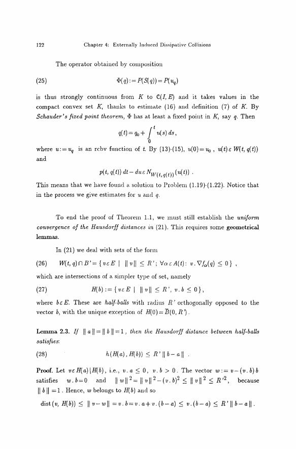
122 Chapter 4: Externally lnduccd Dissipative Collisions

The operator obtained by composition

(25) <I>( q): = P(S( q)) = P( 1tq)

is thus strongly continuous from K to e(J, E) and it takes values in the

compact convex set K, thanks to estimate {16) a.nd definition (7) of K. By

Schauder's fixed point theorem, <I> has a.t least a fixed point in K, say q. Then

t q( t) = q0 + j u( s) ds,

0

where u:=uq is an rcbv function oft. By (13)-(15), u(O)=Uo, u(t)E W(t, q(t))

and

p(t, q(t)) dt- dttE NW(t,q(t)) (u(t)) .

This means that we have found a solution to Problem (1.19)-(1.22). Notice that

in the process we give estima.tes for ·u a.nd q.

To end the proof of Theorem 1.1, we must still establish the uniform

convergence of the Hausdorff distances in {21 ). This requires some geometrica.l

lemma.s.

In (21) we deal with sets of the form

(26) W(t,q)nB'= {vEE I llvll :S: R'; 'iaEA(t): ·u.\lf0 (q) :S: 0},

which are intersections of a simpler type of set, na.mely

(27) H( b) : = { 'V [ E I II VII :s: R , ' 'V. b :s: 0} )

where bE E. These are half-ba.lls with raclius R' orthogonally opposed to the

vector b, with the unique exception of H(O) = B(O, R ').

Lemma 2.3. If II a II = II b II = 1, then the Hausdorff distance between half-balls

satisfies:

(28) h(H(a), H(b)) :S: R' II b- a.ll ·

Proof. Let vEH(a)\H(b), i.e., v.a. :S: 0, v.b > 0. The vector w:= v-(v.b)b

satisfies w.b=O and llwll 2 = llvf-(v.b)2 :S: llvll 2 :S: R'2 , because

II b II = 1 . Hence, w belongs to H( b) and so

dist(v, H(b)) :S: llv-wll =v.b=v.a+v.(b-a) :S: v.(b-a) :S: R'llb-all-

4.2 Existence of a solution 123

We deduce that e(H( a), H( b)) :::; R' Jl b- a Jl. Exchanging b and a, the result

follows. D

The next lemma anses by a detailed inspection of the study of the

intersection of multifunctions clone by Moreau in (Mor 7], § 7.

Lemma 2.4. Let Ai, Bi (1 :::; i:::; n) be convex sets with nonempty interior, all of

them contained in the ball B'=B(O,R'). Let A:=A1n ... nAn and

B: = B1 n ... n Bn .

( a) /f A contains a ball with radius r and if for eveT1J i

(29)

then we have

(30)

(b) /f A contains a ball w-ith radius r and B conta.ins a ball with radius r' and

if for every i

(31)

then the following estimate holds:

(32) h(A,B):::; (~+ 4~')n-l t h(Ai,Bi). - r i=l

Proof. We only need to prove (30), by incluction on n.

For n = 2, our argument is similör to [l\1or 7], Proposition in § 7. Let a

be the center of a ball of radius T contained in the set A = A1 n A2 . In

particular, ac; A1 and dist( a., E\ A2) ;::: r. By (29), there is b1 c; B1 such that

(33)

Since B2 has nonempty interior, we may use (6) in [Mor 7] (see Proposition

0.4.5) and (29) to obtain

(34) dist(a,E\B2);::: clist(a,E\A2)-e(A2,B2) > r-;i=ir.

On the other hand,

(35)

Taking tagether (33)-(35) yields:

(36)

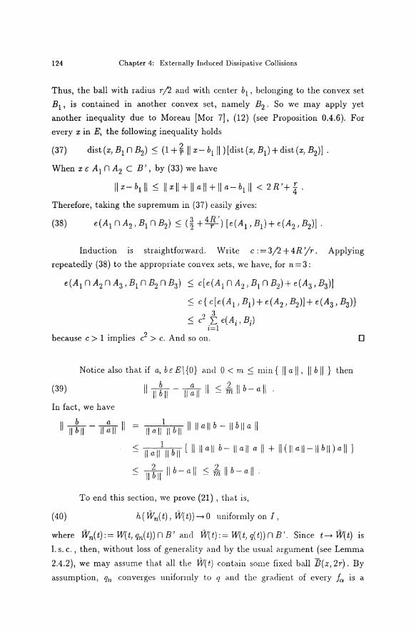
124 Chapter 4: Externally Induced Dissipative Collisions

Thus, the ball with radius r/2 ancl with center b1 , belanging to the convex set

B1 , is contained in another convex set, namely B2 . So we may apply yet

another inequality due to Moreau [Mor 7], (12) (see Proposition 0.4.6). For

every x in E, the following inequality holcls

(37) dist (x, Bl n B2) ~ (1 +~ II x- blll )[clist (x, Bl)+ clist (x, B2)].

When XE Al n A2 c B', by (33) we have

Therefore, taking the supremum in (37) easily gives:

(38)

Induction is straightforwarcl. Write c: = 3/2 + 4R 'jr. Applying

repeateclly (38) to the appropriate convex sets, we ha.ve, for n = 3:

e(A 1 n A2 n A3, B1 n B2 n B3) :::; c[e(A 1 n A2 , B1 n B2) + e(A3 , B3)]

:::; c{c[e(A 1 ,B1)+e(A2 ,B2)]+e(A3 ,B3)}

•) 3 :::; c~ I:: e(Ai,Bi)

i=l because c > 1 implies c2 > c. Ancl so 011. D

Notice also that if a, b E E\ {0} ancl 0 < m :=; min { II a II, II b II } then

(39) II ufrr - II ~: 11 II ::::: -fu II b- a II . In fact, we have

llufrr-11~/111 = llall1 llhllllllallb-llhllall

< II a.11 1 11 b II [ II II a II b- II a II a II + II ( II a 11-11 b II) a II l 2 2 ~ N II b-all ~ m II b-all.

To end this section, we prove (21) , tha.t is,

(40) h ( W11 ( t), W( t))--> 0 uniformly on I,

where W11(t):=W(t,q11(t))nB' ancl W(t):=W(t,q(t))nB'. Since t-->W(t) Js

l. s. c., then, without loss of generality and by the usual argument (see Lemma

2.4.2), we may assume that all the W(t) contain some fixed ball B(x, 2r). By

assumption, q11 converges unifonnly to q ancl the graclient of every fo. is a

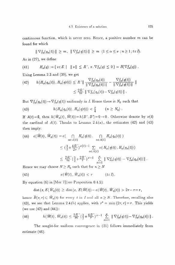
4.2 Exist.ence of a solut.ion 125

continuous function, which is never zcro. Hence, a positive number m can be

found for which

As in (27), we define

{41) Ho.(q) := { 'VE E I II 'VII ~ R', V. \lfcr(q) ~ 0} = H(Vfo.(q)).

Using Lemma 2.3 and (39), we get

V/, (q (t)) Vfa(q(t)) (42) h(Ho.(q11(t)), Ha(q(t))) ~ R 'II II Vf:(q:(t)) II - II Vfo.(q(t)) 11 II

~ 2/J '11 \lfn(!Jn{t))- Vfo.(q(t)) II·

But Vfo.(q11(t))-+ Vfn(q(t)) uniformly in I. Hence there is N0 suchthat

( 43)

If A(t)=0, then h(W11(t), W(t))=h(B',B')=0--+0. Otherwise derrote by v(t)

the cardinal of A( t). Thanks to Lemma 2.4 ( a), the estimates ( 42) and ( 43)

then imply:

(44) e(W(t), Wn(t)) = e( n H(l(q(t)). n Hn(!Jn(t))) crc.-l(i) oc.-1(1)

~ (~+\~') 11 (1}- 1 L e(Hn(q(t)),H0 (q 11(t))) - ~ oEA(t)

~ 2r~·n+ 2rlv-I t IIVJ.}(q(t))-Vfa(q"(t)lll· er=!

Hencc we may choose N ::0: N0 such that for n ::0: N

(45) e( W(t), ~V11 (t)) < r ( tc I).

By equation (6) in [Mor 7] (see Proposition 0.4.5 ):

dist(x,E\Wn(t)) ::0: clist(x, E\W(t))-e(W(t), Wn(t)) > 2r-r=r,

hence B( x, r) C Wn( t) for every t in I and all n :2 N. Therefore, recalling also

(43), we sec that Lemma 2.4(h) applies, with r* = min{2r,r}=r. This yields

(we use (42) ancl (44)):

- - 2R' :l 4R' v-1 v (46) h(W(t), Wn(t)) ~ rn-h+----r) L IIVfo(q(t))-\lfo.(qn(t))ll·

- o=1

The sought-for uniform convcrgcnce iu (21) follows immecliately from

estimate (46).

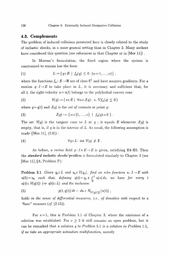
126 Chapter 4: Externally lnduced Dissipative Collisions

4.3. Complements The problern of induced collisions presented here is closely related to the study

of inelastic shocks, in a more general setting than in Chapter 3. Many authors

have considered this question (see references in that Chapter or in [Mor 11]) .

In Moreau' s formulation, the fixecl region where the system is

constrained to remain has the form

(1} L:={qcE I fer(q) :<:; 0 (a=1, ... ,v)},

where the functions fer: E->IR are of dass e1 ancl have nonzero gradients. Fora

motion q: I--> E to take place in L, it is necessary and sufficient that, for

all t, the right-velocity u = u( t) belongs to the polyheclral convex cone

(2} V(q):={vcEI 'Vacl(q): v.\lfer(q) :<:; 0}

where q= q(t) and J(q) is the set of conta.cts at point q:

(3) J(q) := {ac{l, ... ,11} I fer(q)=O} ·

The set V(q) is the tangent cone to L at q ; it equals E whenever J(q) is

empty, that is, if q is in the interior of L. As usual, the following assumption is

made ([Mor 11], (2.6)):

(4) 'Vqc L: int V(q) i 0.

As before, a vector fielcl p: Ix E---> E is given, satisfying H4-H5. Then

the standard inelastic shocks'problcm is formulated similarly to Chapter 3 (see

[Mor 11],§8, Problem P):

Problem 3.1. Given q0 cL and 1/.of V(q0 ), find a.n rcbv function u: J-.E with

u(O)=Uo such tha.t, defining q(t)=q0 + J1 u(s)ds, we ha.ve for every t 0

u( t) c V( q( t)) ( =? q( t) t: L) and the ·incl-usion

(5) p(t, q(t)) dt- du t: NV(q(t)) (u(t)),

holds in the sense of differential m.ea.sures, i. e., of densities with respect to a

"base" m.easure ( cf. (2.15)).

For v = 1, this is Problem 1.1 of Chapter 3, where the existence of a

solution was establishecl. For 11 ;::: 2 it still remains an open problem, but it

can be remarked that a solut·ion q to Problem. 3.1 is a solution to Problem 1.1,

if we take an appropriate activation mult·ifunction, namely

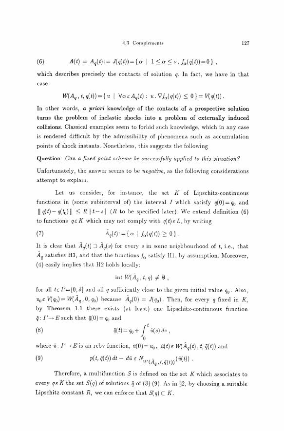
4.:l Co•nplrlllenl.s 127

(6) A(t) = Aq(t):= J(q(t))= {er I 1::; er :S>, JQ(q(t))=O},

which describes precisely the contacts of solution q. In fact, we have in that

case

W( Aq 1 t1 q( t)) = { 1L I V er E Aq( t) : 11.. \1 fo( q( t)) :S 0 } = V( q( t)) .

In other words, a priori knowlcdgc of thc contacts of a prospective solution

turns the problern of inelastic shocks into a problern of cxtcrnally induced

collisions. Classical exarnples seem to forbid such knowledge, which in any case

is rendered difficult by the aclmissibility of phenomena such as accumulation

points of shock instants. Nonetheless, this suggests the following

Question: Can a fixed point scheme be su.ccessfu.lly a.pplied to this situation?

Unfortunately, the answer seems to be negnt-i-ue, as the following considerations

attempt to explain.

Let us consicler, for instance, the set K of Lipschitz-continuous

functions in (some subinterva1 of) the interval I which satisfy q(O) = q0 a.nd

II q(t)-q(la)ll :SR I t-sl (R tobe specified later). We extend definition (6) to functions qc- K which may not comply with q( t) E L, by writing

(7) Äq(t):={er I j 0 (q(t)) 2 0}.

It is clcar that Äq( t) :J Äq( s) for every s in smne ueigh hourhood of t, i .e., that

Äq satisfies H3, ancl tha.t the functions j~ satisfy Hl, by a.ssumption. Moreover,

(4) easily implies tha.t H2 holds locally:

int W(Äq, t, q) fc 0 ,

for all tE 11=[0, .5] a.nd a.ll q sufficiently close to the given initia.l value q0 . Also,

Uo E V( q0 ) = W( Äq, 0, q0 ) beca.use Äq( 0) = J( q0 ) . Then, for every q fixed in K,

by Theorem 1.1 there exists ( at least) one Lipsclli tz-continuous function

q: I'-+E suchthat q(O)= q0 ancl

(8) q(t)=q0 + j 1 1r(s)ds, 0

where u: I'--+ E is an rcbv function, 1/(0) = uv, ü( t) E W( Äq( t) 1 t1 ij( t)) ancl

(9) p(t,ij(t))dt- dil.c- NW(Äq,t,q(t))(1r(t)).

Therefore, a multifunction S is clefinecl on the sct K which associates to

every qE K the set S(q) of solutions q of (8)-(9). As in §2, by choosing a suitable

Lipschitz constant R, we can enforce tha.t S( q) C K.

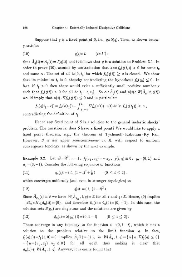
128 Chapter 4: Externally lnduced Dissipative Collisions

Suppose that q is a fixed point of S, i.e., qE S( q). Then, as shown below,

q satisfies

(10) q( t) E L (td');

thus Äq( t) = Aq( t) = J( q( t)) ancl i t follows that q is a solution to Problem 3.1 . In

order to prove (10), assume by contradiction that a: = fa( q( to)) > 0 for some lo and some o:. The set of all tc[O, ta] for which f0 (q(t)) ~ a is closed. We show

that its minimum t1 is 0, thereby contradicting the hypothesis Ja( q0 ) s; 0. In

fact, if t1 > 0 then there woulcl exist a sufficiently small positive number f

such that fa( q( t)) > 0 for all tE [ t1 - f, tj] . So o: f Äq( t) ancl u( t) E W(Äq, t, q( t)) would imply that u( t) . V fa( q( t)) ::; 0 and in particular:

/ 0 (q(tl-t:))= fa(q(tl))- ;;~_, 'V/0 (q(t)). u(t) dt ~ fa(q(tl)) ~ a, I

contradicting the definition of t1.

Hence any fixecl point of S is a solution to the general inelastic shocks'

problem. The question is: docs S have a fixed point? We would like to apply a

fixed point theorem, e.g., the theorem of Tychonoff- Kakutani- Ky Fan.

However, S is not upper sem:icont-in:u.ous on K, with respect to uniform

convergence topology, as shown by the uext example.

Example 3.2. Let E=IR2 ,,;=1; J1(x1 ,2:2)=-:1::2, p(t,q)=:O; q0 =(0,1) and

Uo = (0, -1 ). Consider the following sequence of functions

(11) (0 ::; t s; 2) ,

which converges unifonnly ( ancl even in strougPr topologies) to

(12) q(t):=( t, (1- t)2 ).

Since Äq (t) = 0 we have W(Äq , t, q) = E for all t and qE E. Hence, (9) implies n Jl

-duntNtfun(t))={O}, ancl therefore ·ii.11(t)=ü 11(0)=(0, -1). In this case, the

solution sets S( q11 ) are singletons and the solutions are given by

(13) iin(t)=S(qn)(t)=(O, 1- t) (0 ::; t ::; 2).

These converge in any topology to the function t-+ (0, 1- t), which is not a

solution to the problem relative to thc Iimit function q. In fact,

ft(q(1))=J1(1,0)=0 implies Ä,/1)={1}, so W(Äq,l,q)={ulu.VJ1(q)::; 0}

= { u= ( u1 , u.2) I u2 2 0} for all qE E, thus making it clear that

u11(1) !f. W(Äq, 1, q). Anyway, it is easily founcl tha.t

4.3 Complernents 129

(14) ii( t) = S( q) ( t) = { ((~,·0\,- t), if 0 :::; t :::; 1 if 1 :::; t :::; 2 .

N otice that Äqn ( t) and Aq( t) differ only at t = 1.

This example shows that a sma.ll change in the activation multifunction

t __. A( t) may cause a remarkable change in the solutions to the problern of

induced collisions, say qA . This remark seems to discourage considering an

even bolder fixed point scheme: find an activation multifunction A such that

ÄqA =A.

If we try to solve Problem 3.1 by the discretization techniques of

Chapter 3, then difficulties of simila.r nature arise, which can be traced back to

the fact that the solution to thc gcnr:ml indastic shocks' problern does not

depend continuously on the initial valucs.

Example 3.3. Let E= IR2 , h ( x, y) = - y ancl h( x, y) = x- y; hence the region

where the motion takes place is L={(x,y) : y 2 0, y 2 x}. We take

p(t, q) = 0 ancl u(O) = (1, -1).

If q0(0)=(-1, 1), then the solution q0(t) runs along the cliagonalline in

the second quadrant until it reaches the origin, wherc it remains at rest.

If q,(0)=(-1, 1-c) with 0 < c < 1, then the solution q,(t) runs on a

parallel to that diagonal line, arriving at the axis Ox at the point (1- c, 0),

then follows along this axis up to the origin ancl afterwards it gocs along all the

diagonal line of the first quaclrant.

Hence, if t is large enough, q,(t) does not converge to q0 ( t) as c __. 0.

Concerning the qucstion of uniqucncss of solution for the problern of

induced collisions, similarity with inelastic shocks coulcl suggest that

nonuniqueness is possiblc. On the other hancl, here we cleal with a fixed pre·

assigned activation ( or contact) multifunction, so that uniqueness should not

be discarded right away. The following lines are a unsuccessful attempt to

prove a uniqueness result and are meaut to call attention upon an interesting

technical difficulty.

In order to simplify, we assume that the force fiele! is null p =: 0 and

that the Ievel functions fu belong to e2. Let q = P.u. ancl ij = Pii. be two

130 Chapter 4: Externally Induced Dissipative Collisions

solutions to Problem (1.19)-(1.22). Then q(O) = q(O)= q0 , v.(O)' = ü(O) = Uo and

-duc:NW(t,q(t)/u(t)), -düt:NW(t,q(t))(ü(t)).

Since uniqueness is a local property, without loss of generality we ma.y take

positive numbers k, m, M and r a.nd take ac: E such that, for every t a.nd a:

II u(t) II < M, II ü(t) II < M, 119/o(q(t)) II > m, 119/o(ti(t)) II > m,

llq(t)-q(t)ll < 4kM' l/9fo(q(t))-9/0 (q(t))ll ~ kllq(t)-q(t)ll

and that C( t) ::) B( a, r) and 6( t) ::) B( a, r), where

C(t): = W(t, q(t)) n B(O, M), C(t): = W(t, q(t)) n B(O, M).

These estimates imply that 1L ancl ·ü are also the solutions to the sweeping

processes by C( t) a.ncl C( t). Hence we ma.y a.pply Theorem 2.4.12, inequality

2.4(31 ). Thus:

(15)

where,u(t):=max{h(C(s),C(s)) I O~s~t}.Denoting

Ha(q)={vc:E I llvll ~ M, v.9fa(q) ~ 0},

we notice that, a.s in (2.42)

h(Ha(q(t)), H0 (q(t))) ~ 2rlfll9/o(q(t))-9.fc,(ij(t)) II ~ 2~M II q(t)- q(t) II <;I· Hence, by Lemma 2.4 (b) we get an expression similar to (2.46):

(16) h(C(t),C(t)) ~ 2rlf (~+ 4~Jv-l t ll9fa(q(t))-9fo(ij(t))ll - a=l

~ k* II q( t)- c7( t) II ,

with k*= 2rlf(~+4~)v-lvk.

Define r/J(t):=max { II q(s)- q(s) II : 0 ~ s ~ t}. Then, by (16),

,u( t) ~ k* r/1( t) a.ncl, writing ). : = c k*, ( 15) implies

(17) llu(t)- ü(tJII 2 ~ ).rfJ(tJ.

On the other hancl, we ha.ve

Jt Jt ? l r/1( t) ~ II u( s) - v.( s J II ds ~ ,u [ 11 u( s J - ü( s) II - ds ]2 ,

0 0

by Cauchy-Schwarz inequality. Therefore, using (17):

(18) rjJ(t) 2 ~). t jt rjJ(s) ds.

0

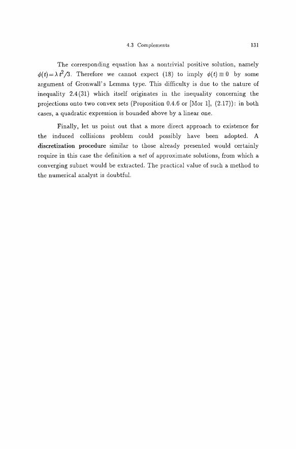
4.3 Complements 131

The corresponding equation has a nontrivial positive solution, namely

<f;(t)=>..t'l!J. Therefore we cannot expect (18) to imply <f;(t):=O by some

argument of Gronwall' s Lemma type. This difficulty is due to the nature of

inequality 2.4 (31) which itself originates in the inequality concerning the

projections onto two convex sets (Proposition 0.4.6 or [Mor 1], (2.17)): in both

cases, a quadratic expression is bounded above by a linear one.

Finally, let us point out that a more direct approach to existence for

the induced collisions problern could possibly have been adopted. A

discretization procedure similar to those alreacly presentecl woulcl certainly

require in this case the clefinition a net of approximate solutions, from which a

converging subnet would be extracted. The practical value of such a methocl to

the numerical analyst is doubtful.

Chapter5

Further Applications and Related Topics

5.1. A dass of second-order differential inclusions Following Castaing [Cas 7], in this section we consider some abstract second­

order differential inclusions to which some of the preceding techniques can be

successfully applied in order to prove existence results. An useful concept is

the following one:

Definition 1.1. A multifunction F from an open suhset D to subsets of the

Hilbert space H is saicl to be anti-monotone if, for all x and y in D and all

uc: F(x) and vc: F(y):

(1) lim llx-y+h(<t-v)ll-llx-yll ::; 0 h...., o- h

or equivalently:

(2) (1L- v). (x- y) ::; 0 (nc: F(x), VE F(y)).

To see that (1) implies (2), write (Iimits are taken as h--> o-):

2( x-y). ( u-v) = lim [ h II n-·u II :! + 2 ( x-y). ('u-v)]

I ·J •J =lim h- ( ll(x-y)+h('u-·u)ll--llx-yii-J

=lim [ II (x-v) + h( u~vl II -11;[:-:v II ( II (x-v) + h( 11.-v) II + II x-y II) l

::; 0.

To see that (2) implies (1) - which is obvious if x= y - assume that

x i= y and wri te as above

!im ll(x-y)+h(<L-u)ll-llx-yll h

I' h II u-v !1 2 + 2 ( x-y). ( u-v) = lnl "II-,( l._._, __ v--;-) --'.+,_,_h(,---·u-.-~v)"l.-1 +"--'-;-;11-'--x---v"'ll

J:-y

= II x-v II . ( u-vJ ::; 0 .

The main existence theorem is the following:

Theorem 1.2. [ Cas 7] Let H be a. Hilbert spo.ce a.nd F: H--> 2H be a

multifunction with nonempty closed con:uex val11.es in H. We assume that F is

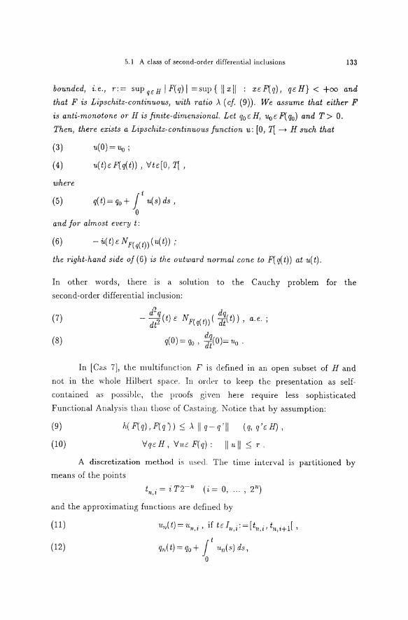
5.1 A class of second-order differential inclusions 133

bounded, i.e., r:= supq<:HIF(q)j =sup{ llxll : xc:F(q), qc:H} < +oo and that F is Lipschitz-continuous, with ratio >. ( cf. (9)). We assume that either F

is anti-monotone or His finite-dimensional. Let q0 c: H, UoC: F( q0 ) and T > 0.

Then, there exists a Lipschitz-continuo·us function u: [0, T[ ~ H suchthat

(3) u(O) = Uo ;

(4) u(t)c:F(q(t)), \ftc:[O, T[,

where t

(5) q(t)=q0 + j u(s)ds, 0

and for almost every t:

(6) - u(t)c: NF(q(t)) (1t(t));

the right-hand side of(6) is the outward normal cone to F(q(t)) at u(t).

In other words, there is a solution to the Cauchy problern for the

second-order differential inclusion:

(7) d2q dq

- dt2 (t) c: NF(q(t)) ( dt(t)) , a.e. ;

(8) q(O) = q0 , ~~(0)= 11ü •

In [Cas 7], the multifunction F is defined in an open subset of Hand

not in the whole Hilbert space. In order to keep the presentation as self­

contained as possible, the proofs given here require less sophisticated

Functional Analysis than those of Ca.staing. Notice that by assumption:

(9)

(10)

h( F(q) 1 F(q')) ~ ). II q- q'll (q, q'd!),

\fqc:H, \f·u.c F(q): II ull ~ r.

A discretization method is used. The time interval is partitioned by

means of the points

... '

and the approximating functions are clcfined by

(11)

(12) q11 (t)=q0 + jt u11 (s)ds, 0

2")

134 Chapter 5: Further Applications and Related Topics

where

(13)

Let us write Bn(t)=tn,i' if t belongs to [tn,i' tn,i+l[. Then, by definition

and from (10)

(14)

So, all the functions qn are Lipschitz-continuous with ratio r and they are also

equibounded: II qn II 00 ~ Q: = II qo II + r T ·

The derivatives un are not Lipschitz-continuous, but the piecewise

affine approximants

(15) vn(t):=un,i+ 2; (t-t 11 ,;)(v.11 ,i+l-u71 ), if tc In,i,

are Lipschitz-continuous, with respective ratios 211 1 1 max II un,i+l- un,i II· Since, by construction, u11 i belongs to F( q11 ( t11 ;) ), we have

' '

so that, by (9) and the above remarks about q11 :

(16) II un,i+l- un)l S: A II qn(tn)- qn(tn,i+l) II ~ -Xrltll,i-tn,i+II=-XrT2-n.

It follows that the Vn are equi-Lipschitz-continuous with ratio Ar:

(17)

From (16) and the definitions it 1s also clear that

II V11(t)- Un(t) II ~ Ar TT 11 , hence

(18) II Vn- "lln II = ---> 0 ·

The anti-monotonicity of the multifunction F is used to pass to the

Iimit, by means of:

Lemma 1.3. IJ F is anti-monotone, then ( q11 ) lS a Ca-uchy sequence for the

metric of uniform convergence.

Proof. Denote by w 111 , 11 ( t) or simply by w( t) tlte quantity ~ II q111(t)-q11( t) 11 2 ,

with m > n. Then:

(tc[O, T[),

5.1 A class of second-orcler clifferent.ial inclusions 135

since Un is the right-clerivative of q". If tc; I)/ in Im]. , then 11-m( t) =um]. belongs ' ' J

to F( qm(tm)) ancl ·u11 ( t) = un,i belongs to P( q11 ( tn:i)). Because F is anti-

monotone (2), it follows that:

( qm( tm)- q11 ( 111 ,;)). (um( t)- ·un( t)) ::::; 0

ancl thus

a;tw ( t) :=::; ( qm( t)- qm( tm)) . ( 1t111( t)- 11-71 ( t)) + ( q11 ( 111,;)- q11(t)) . (Um( t)- Un( t)).

Since (14) holcls ancl since all the q11 have Lipschitz ratio r, we have

d;tw(t)::::; r I t- t111 ,Ji 2r+ r I t11 ,i- t I 2r::::; 2,2 T(2-m+Tn).

Moreover, w(O)=~IIqm(O)-q11 (0)11 2 =0. Hence w(t):s;2,2T(2-m+Tn)t

ancl so 1

II qm- q11 II 00 :=::; 2 r T(Tm + Tn)'l -> 0 ,

when m, n -> + oo , showing that ( qn) is a Cauchy sequence. 0

Before proving Theorem 1.2, let us find an equivalent formulation of

the differential inclusion. In order to do so, we introcluce the following

clefinition:

Definition 1.4. A function ,P: [0, T] x if-> H is callecl an F-selection if it is

measurable, bounded, continuons with rcspect to the H variable and such that

(19) Vtc:[O,T[, Vqc:H: tj;(t,q)c:F(q).

Proposition 1.5. A Lipschitz-contin:rw·ns fnnction u: [0, 7[ -> H which satisfies

conditions (3), (4) and (5) is a sohttion to the differential inclusion (6) if and

only if

(20)

for every F-selection ,P.

JT [,P(t,q(t))-u(t)].it.(t)dt ~ 0, 0

Proof. 1) Let u be a sohttion and ,P be a.n F-selection. Since a.e. - u( t) belongs

to the outward normal cone to F( q( t)) at 11.( t) and since ,P( t, q( t)) c; F( q( t)), it

turns out that

(,P(t, q(t)) -?L(t)). iL(t) ~ 0, a.e.

whence (20).

136 Chapter 5: Further Applicat.ions and Related Topics

2) Assurne that (3)-(5) and (20) hold. We prove (6).

Fix t in [0, 11· For every zc F(q(t)) and every small positive E, we define the

F-selection

<P -{ proj(z, F(q)) (s, q)- proj(u(s), F(q))

if s c [ t, HEl otherwise.

Then <f;(s, q(s))=u(s) if sdt, HE] and (20) implies

Jt+{

t

[proj(z,F(q(s)))-u(s)].u(s)ds ~ 0.

Dividing by E and letting E go to zero, we obtain, for almost every t,

Le.:

[proj(z, F( q( t)))- ·u( t) ]. u( t) ~ 0,

(z-u.(t)).u(t) ~ 0 , a. e ..

Since u(t)c: F(q(t)) and z is arbitrary in F(q(t)), we ma.y conclude that (6)

holds:

-il.(t)c:N F(q(t))(u(t)). D

The first existence result (Theorem 1.2) is provecl next.

Proof of Theorem 1.2. Consicler the approximating sequences ( qn), ( iJn) = ( Un) and ( vn) defined above.

If F is anti-monotone, we have seen (Lemma 1.3) that ( qn) is a Cauchy

sequence for the norm of uniform convergence, hence it converges uniformly to

a Lipschitz-continuous function q.

If H is finite-dimensiona.l, we use instead Ascoli-Arzela' s theorem.

Since ( qn) is a sequence of equi- Lipschitz-continuous functions with the same

initial value, then we may extract from ( q11 ) a sequence that converges

uniformly to a Lipschitz-continuous function q.

Since ( vn) and ( un) are unifonnly bounded in norm and in variation and

since (18) holds, we may suppose (if necessary by taking a subsequence) that

both converge pointwisely weakly to some function u. As every Vn has

Lipschitz ratio .\ r ((17)), we get, using the weak lower semicontinuity of the

norm:

llu(t)-u(s)ll:::; liminfllv11(t)-vn(s)ll·:::; .\rlt-sl;

that is, u is Lipschitz-continuous with ratio .\ r.

5.1 A dass of second-order differential inclusions 137

1. Obviously, u(O)= w-lim u11(0)=·u\J.

2. For every hc: H, q71 • h--) q. h unifonnly, so 11.71 . h= q11 • h --) q. h at least in

the sense of distributions; on the other band, ·n11 • h--) u. h pointwisely, so u= q almost everywhere and (5) holcls.

3. By (9) ancl (14),

dist (u11(t), F(q(t))) ::; h( F(q11(B 71(t))), F(q(t))) ::; A II q11(B 11(t))- q(t) II,

which converges to zero, because B11(t)--) t ancl q11 --) q uniformly. Recalling

that u11 ( t) converges weakly to 11.( t) and that F( q( t)) is a closecl convex set, we

see that ( 4) holds:

u(t) E F(q(t)) .

4. In order to prove (6), we use Proposition 1.5. Let us consider an F-selection

<P and show that (20) holds. Define a 11(t) := tu,i+ 1 if tc:[tn,i, tn,i+d . As

vn( t) = 2n 1 1 ( un,i+l- uu) = 2" 7~ 1 [ proj ( 11n,i · F( IJn( tn,i+1)))- un,i]'

it is clear that - v11 ( t) belongs a.e. to tlw outward normal cone:

N F( qn( tn, i+ 1) )( uu) = NF( qn( er n(t))) ( un( t)) .

By definition of this cone ancl since

</! 11(t) :=1/J(t, q11(a 11 (t))) E F(q71 (a 11(t))),

we have v11( t). [<fn( t)- u11 ( t)] ~ 0 a.e. ancl so:

T T J Vn( t). </J 11 (t) dt ~ J V11 ( t). u11( i) di. 0 0

(21)

Since (v11 ) is bouncled in L=(J, H), we may assume that it convergcs weakly-*

to a function which actually is ·ü.. Moreover, the assumptions on <P and the

convergence q11(a 11(t))--) q(t) imply tha.t <Pn(t)--) <jJ(t, q(t)) =~(t) in L1 norm. It

follows that

and so:

JT v11(t).<jJ"(t)dt--) !Til.(t).<f(t,q(t))dt. 0 0

Concerning the right-hand siele of (21 ), we note that 11.11 - v11 --) 0 uniformly,

v11(t)--) u(t) weakly and v11(0) = 1Jv=1t(O) imply that:

138

T liminf 1

0

Chapter 5: Further Applications and Related Topics

T Vn. Un dt = liminf 1 V11 • Vn dt = liminf ~ ( II vn( T) II 2 - II vn(O) II 2)

0

~~llu(T)II 2 -~IIu(O)II 2 = 1T u(t).u(t)dt. 0

Thus, (21) implies

1r u(t). <P(t, q(t)) dt ~ 0

that is to say (20) . The proof is finished.

1 T u( t) . u( t) dt , 0

0

With standard changes in the rea.soning, a local existence result 1s

obtained for multifunctions defined not in the whole space H, but only in some

open subset of it (see [Cas 7]).

W e give another existence theorem, where the assumptions ( about the

interior) and the techniques remincl us of Chapter 2:

Theorem 1.6. [Cas 7] Let F be a Hausdorff-continuous multifunction from the

Hilbert space H to closed convex subsets with nonempty interior in H. Assurne

that B(a,p)CF(q)CB(O,r), Yqc:H, and that q0 c:H, UoEF(q0 ) and T>O.

Suppose that one of the following conditions -is sa.tisfied:

( a) His finite-dimensional; or

( b) F is anti-monotone.

Then, there exists a continuo·us Junction of bounded variation u: [0, 1{ -t H

suchthat (3) u(O)=vu and (4) u(t)c:F(q(t)) ,\ltc:[O, 1{ hold, where

(5) q(t)=q0 + Jt u(s)ds, andfor I du)-almost every t: 0

(22) - I ~:; 1 (t)c: NF(q(t))(u(t)).

Proof. We define the approxima.nts ( q11 ), ('u.n) and ( vn) as before. Then

II Un(t) II :S: r and the q11 a.re Lipschitz-continuous with constant r and

uniformly bounded by II q0 II + r T. The total variation of un (or vn) 1s

estimated by means of Lemma 0.4.4: since all the sets F( q) contain B( a, p ),

(23) var Un = L II 1tn,i+l- u.n,i II 0:::: i < 211

5.1 A class of second-ordrr differential inclusions 139

If H is finite-dimensional, then by Theorem 0.2.1, Ascoli-Arzela' s

theorem and Lebesgue' s dominated convergence theorem, we may extract a

subsequence, still denoted by ( -un), which converges pointwisely to a bv

function -u (whence -u(O)=~) and suchthat q71(t)=q0 + J~ -u71(s)ds converges

uniformly to a Lipschitz-continuous function q, given by (5). Thus, we have

un( t) c F( qn( Bn( t)) ), un( t) ---> u( t) and also q71 ( B71 ( t)) ---> q( t), because

II qn(Bn(t))- q(t) II ::; II '1n(Bu(t))- '1n(t) II + II qn(t)- q(t) II :Sr I Bn(t)-tl + II q71(t)- q(t) II ---> 0.

These imply ( 4), because Fis continuous.

If H is infinite-dimensional and F is anti-monotone, then Lemma 1.3

yields that ( qn) converges uniformly to a Lipschitz-continuous function

q: [0, T]---> H with ratio r. Extrading a subsequence as in Theorem 0.2.1, we

may assume that u11 = iJ.n converges pointwisely weakly to a bv function u,

which again satisfies (3) and (5 ). Since un( t) converges weakly to u( t),

qn(Bn(t))--->q(t) and Fis continuous with weakly closed values, then

u( t) t: F( q( t)) still holds.

We prove below that in fa.ct (-u.n) converges uniformly to u and that u is

continuous. Thus, as the multifunetiou t---> F( q( t)) is continuous with closed

convex values having nonempty interior, Lemma. 2.2.4 a.pplies: the differential

inclusion (22) is equivalent to

(24) I ·) I ') z.(u(t)-·u.(s))?: 2ll11(t) 11--211 u(s) 11-,

for every s < t and zt: F(q(r)), Vu[s, t].

By continuity of u, we may a.ssume that s a.nd t are multiples of 2-n T

for n !arge enough, so tha.t u11(Bn(s))=n11(s)---> 11.(s) and similarly

Un(Bn(t))---> u(t). Notice also tha.t dist(z,F(q11(r))) :=; h(F(q(r)),F(qn(T)))--->0, uniformly; hence the sequence of functious

cP 11( T): = proj ( z, F( q11( T))) (u[s,t])

converges uniformly to z. For the discretization nodes contained in [ s, t], we

have

(un,i+l-cPn(t",i+l)).(u",i+l-un) :S 0,

since cPn(tn,i+ 1) belongs to F(q71(t11 ,i+l)) and ·un,i+l is the projection of u11,;

in this set. Hence:

140 Chapter 5: Further Applications and Related Topics

z.(Un(t)-un(s)) = z. L: (un,i+l-un)

~ L (z-</>n(tn,i+1)) · ( un,i+1- un) + L un,i+1 · ( un,i+l- un)'

so that, by (23) and §2.3(20):

z.(un(t)-Un(s)) ~ -su~ llz-<f>n(T)II L: llun,i+1-un)l

+ ~ L ( II un,i+l 11 2 - II un,i 11 2)

~- C II z-</>n II oo+~ II Un(t) 11 2 -~ II un(s) 11 2 ·

Passing to the Iimit as n-+oo, we obtain (24) as needed.

In order to complete the proof, Iet us first note that, if ( u11 ) converges

uniformly to u, then so does the sequence of continuous functions ( vn), hence

u is continuous. In fact, we have:

(25) II Vn-Un II oo = max II un i+1- uni II l 'I I

:::; max h(F( qn( t11 )), F( qn( tn,i+l))) -+ 0 . I

Given t > 0, for every t we take 5( t) > 0 such that II x- q( t) II < 5( t) implies h(F(x), F(q(t))) < E/2. The set q([O,T]) is compact, so there isafinite

open covering, denoted by l1 = B(q(t1)1 5(t1)/2) U ... U B(q(tp) 1 5(tp)/2).

Since ( q11 ) converges uniformly to q, then 2-n T < min5( tk)/2r and qn( t) c: l1

for all t and for !arge enough n. Thus, for every i, there is tk such that

II qn(tn)- q( tk) II < 5( tk)/2 , while II q11(tn,i+ J- q11(t11 ) II :::; rTn T < 5( tk) /2.

So, II qn(tn,i+1)- q(tk) II < 5(tk). Hence, for !arge enough n,

h(F(q11(tn,i+l)), F(qn(tn,;))):::; h( F(q11(tn,i+1)), F(q(tk)))+h( F(q(tk)) 1 F(qn(tn1;)))

< €.

This proves (25). The same argument ensures that, if m and n (m > n)

are !arge enough, then

(26)

for every i and j with I11 , j n Im, i =/= 0.

Let t c: [tm,i I tm,i+l[ n [tn,j I tn,j+d. Wehave

um( t) =um i = proj ( um(tm i-l), F( qm(t111 ;))) and J ., '

Un( t) = un, j = proj ( u11 , j-1 1 F( q11 ( t 11 , jl)) = proj ( u11( t111 , i-1) 1 F( q11(t11 ))) ,

smce either tm i = tn 1- and u11(tm i-l) = u11 1-_ 1 or t111 i > tn 1- and 1. J 'I I J J

Un(tm,i- 1)=un,j. Taking (26) into account, the inequality of Moreau about

5.2 Lipschitz approximat.ions of swecping processes 141

projections into convex sets (Proposition 0.4.7) yields :

II um( t)- un( t) II 2 :S II um(tm, i-1)- un(tm, i-1) II 2

+ 2€[ ll·um(t)- ·um(tm i-1) II + II U,l(t)-un(tm i-1) II]. , ,

By induction, we easily see that:

llum(t)-u11(t)11 2 :S 2e[var(·nm;O,t)+var(u11 ;0,t)] :S 4CE.

Hence II um- u11 II 00 --> 0, as m, n--> oo and ('un) converges uniformly. D

5.2. Lipschitz approximations of sweeping processes

Our purpose here is to give an overview of works by Valadier [Vall-3]and by

Gavioli [Gav] on approximations of multifunctions from the interior and from

the exterior, respectively, by more regular ones (c. g. Lipschitz). These

approximations are used to give new proofs of the existence of a solution to a

sweeping process. En passant, we shall need some mathematical tools, unused

in the foregoing; in this context, a reference to [Cas 8] shoulcl be made.

For completeness, Iet us prove existence for the Lipschitz case. The

result is due to Moreau [Mor 2, 9] and the proof is that of [ Cas-Val] Theorem

VII-19 or [Val 2] Theoreme 2.

Theorem 2.1. Let H be a (separablc) Hilbert space, Iet C: [0, T]--> 2H be a

multifunction with nonempty closed convex val11.es and ac; C(O). Assurne that C

is Lipschitz-continuous for the Hausd01jf distance:

h(C(t), C(s)) :SkI t-s I, V t, sc [0, T].

Then there is a unique Lipsch-itz-cont-in-no11.s Jnnct·ion <L: [0, T] --> H such that:

(1) u(O)=a;

(2) \lt,u(t)c;C(t);

(3) -1 ~~~ (t)c;NC(t)(u(t)), a .. e. t.

Moreover, we have:

(4) II ~~t II ::::: k, a.e.

and if, for some zc Hand r > 0, C(t) ::) B(z, r) \lt, then

142 Chapter 5: Further Applicat.ions and Rclated Topics

(5) var(u; 0, T)= j I~~~ I dt :S: l(r, II a-zll) :S: L.ll a-zll 2 .

Proof. Uniqueness is a consequence of the monotonicity of x---> N C(t) (x).

For existence, assmue with no loss of generality that T= 1 (to simplify

some expressions ). For n :::: 1 , define the polygonal function Xn first on the

set Dn of points i2-n by

and then on the intervals ]( i-1 )2- 11 , i 2- 11 [ by affine interpolation. Derrote

un(O)=O, un(t)=i2- 11 if tc; ](i-1)2- 11 ,i2- 11]. In each one of the above open

intervals, the derivative x;1 is consta.nt:

and we have

-x'n(t) c NC(i 2-n)(x11(i2- 11 ))= NC(<Tn(l))(x11(u 11(t))),

II ~(t) II = 211 dist (x11((i-1) 2-"), C( iT")) :S: 211 h( C(( i-1) 2- 71 ), C( iT11))

::; 211 k2-1l = k.

This allows the extra.ction of a. suhsequence ( <t~) from ( :1,1) such that the

sequence of derivatives (u~,) converges u(L1J,L}1) to ·u'cL00(0,l; H) with

II u'( t) II :S: k a.e .. The corresponclent subsequence of ( x71 ) is denoted by ( up)

Let ! I u(t)=a.+ ·u.'(s)ds.

0

If t belongs to D = U D" , theu ·n1A t) E C( t) for every p !arge enough n and, since up(t)---> u(t) weakly, we have u(t)c C(t). Since u and C are

continuous and since D is dense in [0, 1] , we reaclily obta.in property (2).

Denote by 6(x I C) the indicator funct·ion of a convex set C (which IS

zero on C and += outside) and by o*(x' I C) its support function

( = sup { x'. x I xc C} ) . Consider the functionals

I(v) = j 1 6*(-u( t) I C( t)) dt (vc L00(0, 1; HJ), 0

I*(w)= j 1 6(w(t) I C(t)) dt (wcL1(0,l; H)). 0

According to [Roc 1] (for separable H) or [Cas-Val](Theorem VII-14) these are

mutually polar ( conjugate) functionals, hence they are both weakly lower

5.2 Lipschitz approximations of swecping processes 143

semicon tin uous.

If zc: L00 , then 11 z(t). ( 1 t z(s) ds) dt=! II 11 z(t) dt II 2 , by Fubini's 0 0 0

theorem. Thus, the functional

z-+q(z):= 11 z(t).adt+!ll 11 z(t)dt11 2

0 0 1 is weakly lower semicontinuous in 1= and satisfies q( u~) = 1 u~( t). up( t) dt

= < U~ 1 Up >. 0

Let n= np be such that 11.~ = x;,P. We recall that (see e. g. [Cas-Val]

Theorem II-18):

IS*(x'l C)-S*(x'l CJI:::; llx'll h(C,C).

By the assumptions on C, we have:

11 11 I S*(- u~(t) I C(t)) dt- S*(- u.~,(t) I C(an(t))) dt I :::; 0 0 l

:::; k2 1 I an(t)-tl dt j

0 again using II u~( t) II :::; k a.e. , we also have:

11 11 I u'p( t) . up( t) dt- ·u~( t) . up( a n(t)) dt I 0 0

? 11 :::; k- I an( t)- t I dt . 0

Moreover, in the open subintervals, - ·u~(t) belongs to the outward normal

cone to C(an(t)) at up(a11(t))=x11(a"(t)) (where n=np) and this can be

expressed also by the geometrically clear condition

From the above considerations, it follows that:

I(- u~ ) + < u;, '"lf-p > :::; 21.:2 1 I I an( t)- t I dt = T 71 k2 '

0

whence, by the lower semicontinuity of I ancl q:

I(-u')+ < u',u> = 11 [S*(-u'(t) I C(t))+u'(t).u(t)]dt:::; 0. 0

But (2) and the definition of the support function imply that

S*( -u'( t) I C( t)) 2': - u'( t). -u( t). Hence, we must have:

S*( -u'( t) I C( t)) ==- v.'( t) . u( t) a.e. ,

which, taken tagether with (2), means that (3) holcls (by a well-known result

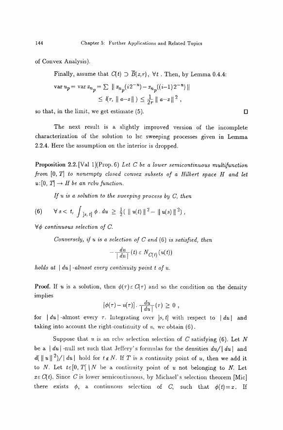
144 Chapter 5: Further Applications and Related Topics

of Convex Analysis).

Finally, assume that C(t) :J B(z,r), Vt. Then, by Lemma 0.4.4:

varup=var:~:n =L: 11:!71 (i2-n)-:~:n ((i-l)Tn)ll p p p

~ l( r, II a-z II ) ~ ir II a-z II 2 ,

so that, in the limit, we get estimate (5). 0

The next result is a slightly improved version of the incomplete

characterization of the solution to lsc sweeping processes given in Lemma

2.2.4. Here the assumption on the interior is dropped.

Proposition 2.2. [Val 1 ](Prop. 6) Let C be a lower semicontinuous multifunction

from [0, T] to nonempty closed convex subsets of a Hilbert space H and let

u:[O, T] ~ H be an rcbv function.

If u is a solution to the sweeping process by C, then

(6) Vs< t, j]s,t]cf>.du ~ !( llu(t)11 2 -llu(s)ll 2),

Vc/> continuous selection of C.

Conversely, if u is a selection of C a.nd (6) is sa.tisfied, then

- I~~: I (t) E NC(t) (1t(t))

holds at I du I -almost every con.t-inuity point t of u.

Proof. If u is a solution, then 4>( r) c: C( r) and so the condition on the density implies

[4>(r)- u(r)J. I~~ I (T) ~ 0 ,

for I du I -almost every T. Integra.ting over ]s, t] with respect to I du I and taking into account the right-continuity of u., we obtain (6).

Suppose that u is an rcbv selection selection of C satisfying (6). Let N be a I du I -null set such that Jeffery' s formulas for the densities du/ I du I and

d( II u 11 2)/1 du I hold for t 1!: N. If T is a continuity point of u, then we add it to N. Let tc:[O, T[ \ N be a continuity point of u not belonging to N. Let

xc: C(t). Since Cis lower semicoutinnous, by lVIichael' s selection theorem [Mic]

there exists 4>, a continuons selcction of C, such that 4>( t) = x. If

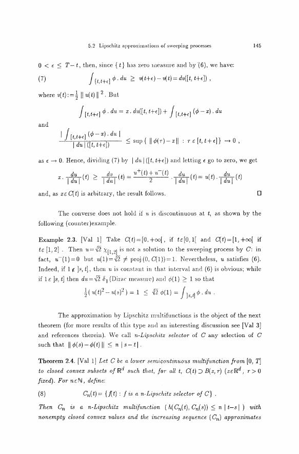
5.2 Lipschitz Rpproxirnat.ions of sweeping processes 145

0 < c :::; T- t, then, since { t} has zero l!leasme and by ·( 6), we have:

(7) j(t,t+t]<jJ.du 2 v(t+c)-v(t)=dv([t,t+c]),

where v(t):=! II u(t) 11 2 . But

j(t,t+t] ,P.du= x.du([t,t+c])+ j(t,t+t] (,P-x).du

and

I J (I, t+t l ( rP - X) . d1t I . I du I ([ t, t+<]) :S; sup { II cP( T)- x II . T c: [ t, t + 1::)} -> 0 ,

as 1::--> 0. Hence, dividing (7) by I du. I ([t, t+c]) and letting c go to zero, we get

du ( dv -u+(t) + ·u.-(t) du ( () du () X.~ t) 2: ~~(t) = 2 ·~ t)= U t ·~ t

and, as xc: C( t) is arbitrary, the result follows. 0

The converse does not hold if 1t is discontinuous at t, as shown by the

following ( counter )example.

Example 2.3. [Val 1] Take C(t)=[O.+oo[, if tc:[0,1[ and C(t)=[1,+oo[ if

tc: [1, 2] . Then u=~ X[t,:2] is not a solntion to the sweeping process by C: in

fact, u-(1)=0 but u(1)={:2 f proj(O,C(1))=1. Nevertheless, u satisfies (6).

Indeed, if 1 f. ]s, t], then u is constant in that iutcrval and (6) is obvious; while

if 1 c: ]s, t] then du= {:2 S 1 (Dirac me<tsme) and cP( 1) 2 1 so that

I ·J ·J rc> J 2( 1t(t)- -1t(s)-) = 1 :S; ~2 </>(1) = ]s,l] ,P. du.

The approximation by Lipschitz multifunctions is the object of the next

theorem (for more results of this type and an interesting cliscussion see [Val 3]

ancl references therein). 'vVe call n-Lipsch:itz selector of C any selection of C

suchthat llci>(s)-<jJ(tJII :S; nls-tl.

Theorem 2.4. [Val 1] Let C be a lower serniqontimta1ts m.ultifunction from. [0, T]

to closed convex subsets of IR!d s-u.ch tlw.t, j&r· oll t, C( t) ::J B( z, r) ( zc: IR!d, r > 0

fixed). For nc:N, define:

(8) C71 ( t) = { f( t) : f is a n-Lipschitz selector of C} .

Then Cn is a n-Lipschitz m.1dtijunct1on ( h(C11(t), C11(s)) :S; n I t-sl) with

nonem.pty closed convex values and the increa.sing sequence ( C11 ) approxim.ates

146 Chapter 5: Further Applical.ions and Related Topics

C in the following sense:

(9) Vt, int C{t) C U Cn(t) C C{t); neN

in particular, C( t) is the closure of the union of all the Cn(t).

Proof. It is obvious that z e C11( t) c C( t) and that C11(t) c Cn+l ( t) .

Since a convex combination of n-Lipschitz selectors of C is still a n­

Lipschitz selector, we see that C11(t) is a convex set. lf x is the limit of (A(t)), where (A) is a sequence of n-Lipschitz selectors, then extracting (by Ascoli­

Arzela' s theorem) a subsequence converging uniformly to some function f and

observing that f is a n-Lipschitz selector of C and x= .!{ t), we prove that Cn(t)

is a closed set.

To show that Cn is a n-Lipschitz multifunction, take an arbitrary

x=J{t)c: Cn(t) and, since dist (x, C';b)) :S II .l{t)- j{s) II :S n I t-s I, conclude

that e( Cn( t), Cn( s)) :S n I t-s I and, by symmetry, h( Cn( t), Cn( s)) :S n I t-s I . It remains to prove that if x is in the interior of C( t) then it belongs to

some Cn(t). Because C is lower semicontinuous, by Lemma 2.4.2 there is a

neighbourhood V oft such that x belongs to the interior of C{s), for all s in V. Let o:: [0, T] --+ [0, 1 J be a Lipschitz-continuous function whose support is

contained in V, with o:(t)=l. Then j{s)=o:(s)x+(l-o:(s))z IS a Lipschitz-

selector of C and .!{ t) = x. 0

We shall also need to approach unifonnly a selection of C by selections

of the approximate multifunctions C11 •

Proposition 2.5. [Cas S](Prop. 2.5) Let ( C11 ) be an increasing sequence of

continuous multifunct-ions from [0, T] to closed convex subsets of fRd, converging

to a multifunction C in the following sense:

C{t)=cl(U C,.(t)), Vt. n

If <P is a continuous selection of C, then there exists a sequence ( <Pn) which

converges uniformly to <P and S1tch. that, for every n, <Pn is a continuous

selection of Cn .

Proof. Define rn(t) = dist (<P(t), C11(t)). These are continuous functions (<P and

Cn are continuous). For every t, r11(t) is a nonincreasing sequence (because

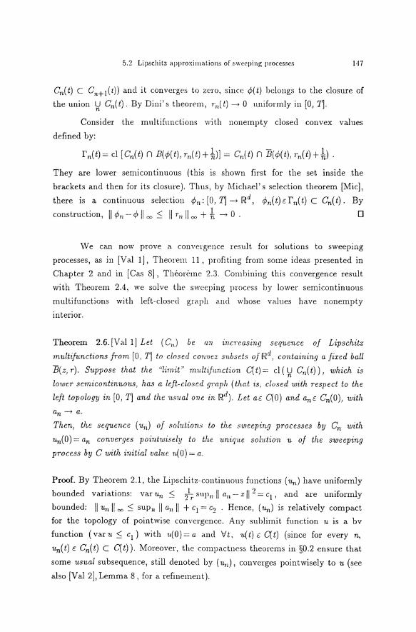
5.2 Lipschitz approxillull.iolls of swerping processes 147

C11(t) C C,.+1(t)) ancl it converges to zero, since <f;(t) hdongs to the closure of

the union U C11(t). By Dini' s theorem, 1'n( t) -> 0 uniformly in [0, T]. n

Consicler the multifunctious with nonempty closecl convex values

clefinecl by:

1 - 1 rn(t)= cl [Cn(t) n B(</;(t), rn(tJ+nJJ = Cn(t) n B(<f;(t), r,.(t)+n;).

They are lower semicontinuous ( this is shown first for the set inside the

brackets ancl then for its closure ). Thus, by lVIichael' s selection theorem [Mic],

there is a continuous selection </; 11 : [0, T] -> IRd, </;11( t) t: rn( t) C C11( t). By

construction, II <Pn- <P II 00 :S II rn II 00 + ~ -> 0 . D

We can now prove a convergence result for solutions to sweeping

processes, as in [Val 1], Theorem 11, profiting from some icleas presentecl in

Chapter 2 ancl in [Cas 8], Theoreme 2.3. Combining this convergence result

with Theorem 2.4, we solve the sweeping process by lower semicontinuous

multifunctions with left-closecl graph and whose values have nonempty

interior.

Theorem 2.6. [Val 1] Let ( C11 ) be an increa.sing seqv.ence of Lipschitz

multifunctions from [0, T] to closed con·uex snbsets of IRd, containing a. fixed ball

B(z, r). Suppose that the "Iimit'" multifu.nction C( t) = cl ( U C71 ( t)), which is n

lower semicontinuous, ha.s a left-closed g1'a.ph ( that is, closed with respect to the

left topology in [0, T] and the 1Lsv.al one in IRd). Let at: C(O) and a11 t: C11(0), with

a11 -> a.

Then, the sequence ( u11 ) of solut·ions to the sweeping processes by C11 with

u,.(O) = a11 converges pointwisely to the unique solution u of the sweeping

process by C with init·ial valv.e 11.( 0) = a.

Proof. By Theorem 2.1, the Lipschitz-continuous functions (1111 ) have uniformly

bounded Variations: var u11 ::; 21 r sup" II a11 - z 11 2 = c1 , and are uniformly

bounded: II u,. II 00 :S sup,. II a.11 II + c1 = c2 . Hence, ( u11 ) is relatively compact

for the topology of pointwise convergence. Any sublimit function u is a bv

function (varu:Scj) with ·u.(O)=a. and Vt, 11.(t)c:C(t) (since for every n,

u,.(t) t: C11(t) C C(t) ). Moreover, tl1e compactness theorems in §0.2 ensure that

some usual subsequence, still clenotecl by (-u11 ), converges pointwisely to u (see

also [Val 2], Lemma 8, for a refinement ).

148 Chapter 5: Further Applications and Related Topics

I) We show that u is right-continuous at every te[0 1 1[.

Let c > 0. Since u( t) c C( t), by Lemma 2.4.4 there is some Xo c C( t) and

some r0 > 0 such that l(r01 l!u(t)-:z:oll) :S 2~ llu(t)-:z:o11 2 < f and - 0 B(:z:o 1 r0 ) C intC(t). The multifunction n---tC71(t), if extended to n=oo by

C=(t)= C(t), is lower semicontinuous at infinity. Then, Lemma 2.4.2 implies

that, for !arge n, C71 ( t) contains the closed ball B( Xo 1 r0 ) in its interior;

moreover, we may ensure that l( r0 1 II u 71 ( t)- Xo II ) < € holds for n ~ N. By

the lower semicontinuity of CN and Lemma 2.4.2, take 8 > 0 in such a way

that CMr) ::J B(:z:o, r0 ) , \h c [t, t+8]. This still holds with N replaced by

n ~ N, so that the estimate in Theorem 2.1 implies:

It follows that

\j T e [ t1 t+8], ll11.( r)- 'U.( t) II :::; va~· ( 1Lj t, t+8) :::; f .

2) We show that u is left-continuous at every t c ]0 1 T].

Taking t71 converging to t from the left, we see that ( fn 1 u( fn)) c graph C

converges to (t1 u-(t)); since the graph of Cis left-closed, we then conclude

that u-(t) c C(t). Let € > 0. The arguments in 1), if applied to u-(t) and to an

interval to the left of t, show that there exists a ball B( x1 1 r1) such that

1h 1 llu-(t)-x1 11) < E and that, for !argen, B(x11 r1)c C71(r), \/rc[t'1 t]

where t 1 < t. Moreover, by taking !arger t' and n if necessary, we have

llu(t')-u-(t)ll < E, l(r1 , 111L(t')-x1 11) < E, llu11(t')-u(t')ll <fand so

(Theorem 2.1) 111L71(t)-u.71 (t')ll :S var(u.n; t,t 1) :S l(rl, llun(t')-xJII)< €.

Then, by the tria.ngle inequality: 111L11 ( t)- u-( t) II < 3 E and, in the Iimit,

II u(t)- u-(t) II :S 3 E. Thus, u-(t) = 1t(t).

3) To end the proof that ·u is the unique solution to the sweeping process

by C starting at a ( and hence that the whole sequence ( u 71 ) has a unique

sublimit and therefore converges pointwisely), we can now apply Proposition

2.2. We only need to establish (6).

Let if;: [0 1 T] ---t IRd be a continuous selection of C and let s < t . From

Proposition 2.5, we may take a sequence ( c/; 71 ) converging uniformly to if;, with

ifin a continuous selection of C11 • Since if; 71 is also a selection of Gm for m ~ n,

then, by the necessary part of Proposition 2.2, ·nm satisfies:

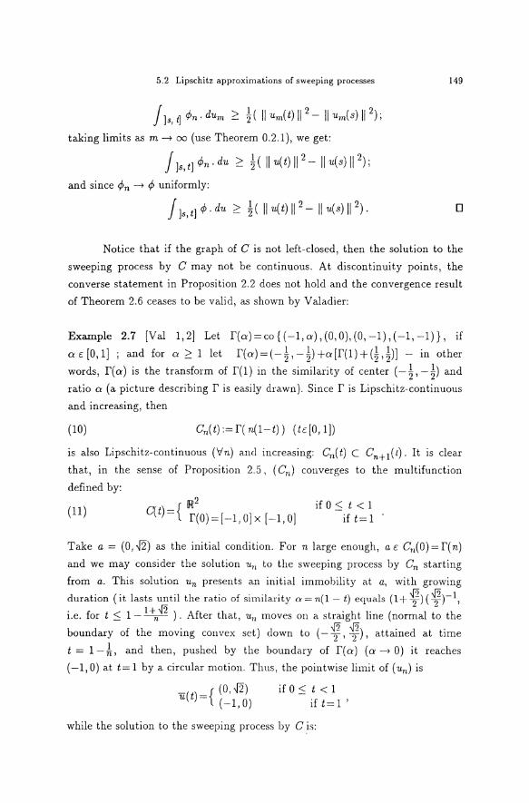
5.2 Lipschitz approximations of sweeping processes

!]s,t] ~n.dum 2.': ~( llum(t)ll 2 -llum(s)ll 2);

taking limits as m ~ oo (use Theorem 0.2.1), we get:

j]s,t]ifJn-du > ~( liu(t)il 2 -llu(s)il 2);

and since ~n ~ ~ uniformly:

j]s,t]~.du > ~( llu(t)il 2 -liu(s)ii 2).

149

0

Notice that if the graph of C is not left-closed, then the solution to the

sweeping process by C may not be continuous. At discontinuity points, the

converse statement in Proposition 2.2 does not hold and the convergence result

of Theorem 2.6 ceases to be valid, as shown by Valadier:

Example 2.7 [Val 1,2] Let f(a)=co{(-1,a),(0,0),(0,-1),(-1,-1)}, if

ac[0,1]; and for a;?:: 1 let f(a)=(-~,-!)+a[r(1)+(!,tlJ- in other

words, r( Q) is the transform of f(1) in the similarity of center (- t)- tl and

ratio a (a picture describing r is easily drawn). Since r is Lipschitz-continuous

and increasing, then

(10) Cn(t):=r( n(1-t)) (tc[O, 1])

is also Lipschitz-continuous (Vn) ancl increasing: C11(t) c Cn+ 1(t). It is clear

that, in the sense of Proposition 2.5, ( Cn) converges to the multifunction

defined by:

(11) IR2

C(t)={ r(0)=[-1,0]x [-1,0] if 0 s t < 1

if t= 1

Take a = (0,{2) as the initial condition. For n !arge enough, ac C11(0)=r(n)

and we may consider the solution <Ln to the sweeping process by Cn starting

from a. This solution Un presents an initial immobility at a, with growing

duration (it lasts until the ratio of similarity o:=n(l- t) equals (1+ ~)(f)- 1 , i.e. for t S 1- l+n..J2 ) . After tha.t, u" moves on a straight line (normal to the

boundary of the moving convex set) down to (- ~, ~), a.tta.ined at time

t = 1-t and then, pushecl by the boundary of -f(aJ (a ~ 0) it reaches

(-1,0) at t=l by a circular motion. Thus, the pointwise Iimit of (un) is

-(t)={ (0,{2) u (-1,0)

if 0 ::; t < 1 if t= 1 '

while the solution to the sweeping process by Cis:

150 Chapter 5: Further Applir.ations and Related Topics

{ (O,.J2) u(t)== (0,0)

if 0 $ t < 1 if t == 1 '

since the projection of (0, .J2) in C( 1) is (0, 0). 0

We now turn our attention to Lipschitz approximations from the

exterior, following Gavioli's work [Gav].

We say that a multifunction Cis rnetrically upper sernicontinuous at t

if r->t implies that e(C(r), C(t))->0, or equivalcntly, iffor every positive e, in

some neighbourhoocl U== U(€) oft:

(12) C(r) C C(t) + d~(O, 1), VTE U.

Theorem 2.8 [Gav] (Theorem 2.1) Let C be a. metrica.lly 1tpper semicontinuous

multifunction from a metric space (I, d) to nonempty bounded closed convex

subsets of a normed spa.ce E. Ass'll.me that C is bou.nded in the sense that

C(t) c B(O, M), V tt: I.

Then, there exist Lipschitz-conti'fi:UO'I/.8 rn:u.ltifnnctions c11 ( n :::: 1 ), of the same

type, with the properties:

(13)

(14)

(15)

C11(t) :> C11+1(t) :> C(t), V te I;

h(C11(t), C(t))-> 0, Vtc I;

h(C11(t), C11 (s)) $ L11 d(t,s), Vt,se I.

The technique is essentia.lly geometrical and the following result JS

needed. For simplicity, we writP B== 73(0.1) .

Lemma 2.9 [Gav] (Lemma 2.1) Let ( ri ); < 1 be a family of nonempty bounded

closed convex subsets of E. Ass-u.me th.a.t all the sets ri contain a fixed ball

B(:ro, h) and write

(16) L==inf lfi-Xol ==infsup llx-:roll 1 xc:f.

I. Then:

(17) n - n L-Ve>O, (fi+eB)c fi+h.eB; id id

i. e., the intersection of enlargcd sets ·is contained in an enlarged intersection of

the sets ri.

5.2 Lipschitz approximat.ions of sweeping processcs 151

Proof. Writing f= n ri and f,= n (fi+cß), we show that, for every u fu I I

there is some X 16 r with II X 1-xll::::; L*, by taking

x 1 := x+ h~c (:ro-x).

In fact, u; r, implies that II x-:ro II ::::; I ri-Xo I +f for every i, hence

llx 1-xll::::; c(h+c)- 1 (L+c)::::; cL/h (since L 2: h). On the other hand, for

every i, there is some xiEfin(x+cB). Then the point zi:=x 1-~(xi-x') satisfies II zi- Xo II = II ~ ( x- xj) II :S h and so zi c r i . Hence, remarking that x 1

is a convex combination of xi and zi, to be precise:

I E + h X = h + E zi h + E Xi '

we conclude that X 1cfi (for every i), i.e., x'c:f. D

The following Lemma contains some properties neecled in the sequel. It

is a particularization of a stanclarcl regnlarization or approximation method for

real functions on metric spa.ces.

Le=a 2.10. Define functions r and rn by r(t1 r):=e(C(t) 1 C(r)) and

rn(t1 r)=~+sup [r(t 1,r)-nd(t,t')]. Thentheysatisfy t 1c I

(18) p > 1'(t, r) =? C(t) C C(r) + p B;

(19) r11(t, r) > r11+ 1(t, r) , 1+2M 2: r11(i1 1) 2: ~+ r(t1 r);

(20) r11 (t. 1) -> e( C(t), C(r));

(21) I rn(t, r)- r11(s, r) I :S n d(t, s) .

Proof. The definition of r( t1 r) as the excess of C( t) over C( r) gives (18). It is

obvious that ( r71 ) is a decreasing sequence. Taking t 1 = t, we obtain

r11(t1 r) 2: ~+r(t,r). Moreover, C(t') U C(r) C B(O,M) implies r(t 1,r)::::; 2M

and so r 71 :S 1 + 2M .

To prove (20), take f > 0 and a positive number {j such that

lr(t 11 r)-r(t1 r)l < E whenever d(t',t)< 8. If n 2: 2Mj8, then d(t'1 t) 2: /j

implies r(t 11 T)-nd(t1 t')::::; 2M-nb::::; 0; so, these t' clo not matter in the

computation of r71 • It follows that

~+r(t,r)::::; r11(t,r)::::; ~+r(t1 r)+c

and eventually I r n( t1 r)- r( t, r) I ::::; 2c, proving convergence.

152 Chapter 5: Further Applications and Related Topics

Writingr71 =r71 -~, we have, for every t'c I:

rn(t,r) ~ r(t',r)-nd(t',t) ~ r(t',r)-nd(t',s)-nd(s,t)'

so that, by taking the supremum

r 71 ( t, r) ~ r 11 ( s, r)- n d( s, t);

exchanging t and s, we obtain I rn(t, r)-r 11(s, r) I :::; nd(s, t) and (21)

follows. 0

We can now proceed with the proof of the approximation theorem.

Proof of Theorem 2.8. Define for every t in the metric space (I, d):

(22) Cn(t)= cl n (C(r)+r11(t,r)B), rcl

a bounded closed convex subset of E.

By the preceding Lemma, (18) ancl (19), r11(t, r) > r(t, r) implies

C11(t) :J C( t). Because r n is nonincrea.sing, the sequence ( C11( t)) is also

nonincreasing, thus proving (13 ).

To prove (14), we fix tc I, < > 0 and, by (20), we choose n so that

r11(t,t) < < for n ~ n. Then C(t) C Cn(t) C cl(C(t)+r11(t,t)B) C C(t)+<B

yields h( C71 ( t), C( t)) :::; t" •

In order to prove that C11 is a Lipschitz-continuous multifunction (claim

(15)) we write

from (21) it follows that:

(23) f 11(s,r) c f 11(t,r)+n d(t,s)B.

The family { r n( t, r) : TE I} fulfils the assumption of Lemma 2.9. Indeed, for

any :rv c C(t), by (18) we have

B( Xv ' 21 ) c C( t) + 21 B c C( T) + ( 1'{ t, T )+ ?1 ) B + 21 B n n _n n

and so, by (1~):

(24) B(:rv,ln) C C(r)+r11(t,r)B=f 11(t,r);

moreover, r 71 ( t, t)- Xo C C( t) + r71( t, t) B- C( t) C [ M + (2M+l) + M] B implies

that:

5.2 Lipschitz approximations of sweeping processes

Hence, by (23) and applying Lemma 2.9 with h= ln and c = n d(t, 8):

n fn(8,T) C n (fn(t,T)+cß) T T

153

c ( n rn(t, T) )+2 nLc B c Cu(t) +2 n2 (4M+ 1) d(t, 8)B. T

Thus Cn( 8) C Cn( t) + Ln d( t, 8) B and a similar inclusion holds when 8 and t

are exchanged. Thus, h( C71(8), C11(t)):::; L11 d(t, 8), with Ln=2 n2 (4M+ 1). 0

According to [Gav], Theorem 2.8 is still true for multifunctions with

"sublinear growth", that is, with I C( t) I :::; M( 1 + d( t, lo)).

A metrica.lly upper semicontinuous multifunction C can thus be

approached by a sequence (C71 ) of Lipschitz-continuous multifunctions for

which there exist solutions (u.11 ) to the sweeping process (Theorem 2.1). If

additionally the multifunction C is Hausclorff-continuous and if C( t) has

nonempty interior (for every t) then it can be shown that ( un) converges

uniformly to the solution to the sweeping process by C:

Theorem 2.11 [Gav](Theorem3.1) Let C be a m·ultiftmction on I=[O, T] with

bounded closed conuex va.lnes in a. sepa.rable Hilbert space H. Assurne that C i8

H ausdorff-contimwus ( i. e., s -> t =? h( C( s), C( t)) -> 0) and that every C( t) ha8

nonempty interior. Take a. scqu.cnce ( Cn) of Lipschitz-continuou8

multifunctions approaching C from the exterior as in Theorem 2.8 and,

a c C(O) being fixed, derwte by 11.11 t!t.e solu.tion to the sweeping proce8s by Cn

with un(O) = a.

Then, ( u11 ) convages 7t.n:iformly on I to a. contimwus bv function u,

which is the solution to the sweepinq proces8 by C with initia.l va.lue u(O) = a.

Proof. As in the proof of Lemma 2.3.2 (b), we may clivide I into a finite

number of intervals Jk = [ tk, tk+ tl such that all the sets C( t) with t in Jk

contain some fixed ball B( a.k , Tk). Since the same can be saicl of Cn( t) - which

contains C(t)- for ncN ancl tt: Jk, then, from Theorem 2.1, (5), we get

var(un,lk):::; (2rk)- 1 1!u11 (t"J-a.kl! 2 . Therefore, it is easily shown by

induction that ( 1L11 ) is unifonnly bonud('d hoth in norm and in variation, say

by M> 0.

We now prove that tlwse Lipschitz-continuous functions converge

uniformly to some function 11., which nmst be continuous and have var u :::; M.

154 Chapter 5: Further Applications and Related Topics

Let m < n. Since um(O) = u11(0) = a, we have

! II U 11(t)-um(t) 11 2 = jt (u11(s)-u 71b)).(u:b)-u:11(s))ds 0

and, by taking um, n( s) to be the projection of um( s) in C11 ( s), we rewrite the

above integral as the following sum:

Jt Jt (25) ( Un(s)- um,n(s)). u~( s) ds + ( Um,n( s)- um( s)). u~( s) ds 0 0 t

+ j (um(s)-Un(s)).u:n(s)ds. 0

The first term is not positive, since ·u.11 solves the sweeping process by C11 and

Um,n is a (continuous) selection of eil (cf. Proposition 2.2). Since

Un(s)c C11(s) C C711(s) ancl um is a solution to the sweeping process by Gm, the

third integral in (25) is also nonpositive. Notice that:

II um,n(s)- um(s) II =clist (u711(s), C11(s))

:=:; clist(u111(s), C(s)) :=:; <Pm(s):= h(Cm(s), C\'s)),

since C11(s) :> C(s) ancl u111(s) c C11b). Tlms, we have

(26) :=:; j t (n111 , 11 (s) -7/."b)). v~1 (s) ds 0

:=:; II <Pm II oo var ( un) :=:; M II <Pm II = ·

The <Pm are continuous functions ( C11 cmd C are continuous multifunctions),

converging monotonically to zero, as m.-+oo (uncler the conclitions of Theorem

2.8, (13), (14)). By Dini's theorem, ll4>mlloo-+ 0. Thus, (26) implies that (Un)

is indeed a uniformly Cauchy hence convergent sequence.

The limi t function 7l satisfies the initial concli tion ancl u( t) c C( t) , since

dist(u(t), C(t))=li;pdist(u11(t), C(t)) :=:; li\ph(C11(t), C(t))=O

and C( t) is closed.

In view of Proposition 2.2, to complete the proof that the cbv function

u is the solution to the sweeping process hy C, we only need to show that (6)

holds for every continuous selcction of C, say yl>. In fact, any such </> is also a

continuous selection of C11 , so:

5.3 An applicat.ion of differential indusions to qua~i-statics 155

Passing to the Iimit (we u~e uniform convergence or Theorem 0.2.1), we get

J I ·J 1 ? ]s,t]fjJ.du 2: 2111t.(t)l!--211u(s)l!-,

as required. D

5.3. An application of differential inclusions to quasi-statics

Following Chraibi [Chr], we study the motion, with respect to an orthonormal

set of Coordinates (0, 71 ,72,73), of a point q(t) (tel:=[O, T]) which is

drawn to a point with knownmotion a(t) by an elastic force F=-k(q(t)-a(t)) where k > 0 is fixed. The point q is to be confined to the half-space

L = { (X 1 ' :z:.1 ' X;j) E IR3 : 2:3 ~ 0 }

by a fixed rigid wall P with eqnation 1::3 = 0. When q comes into contact with

P, we assume that it is suhjectecl to dry friction of Coulomb type, isotropic

but possibly non-homogeneons: the friction coefficient v may clepend on the

position q.

Moreover, we place ourseh·es in a qnasi-statical setting: the mass of q is

taken to be zero. This simplifying a.ssumption is reasonable in many

Engineering applications and it l<·nds to a reduced size of computations.

However, the smoothing efkct of inertia is lost and so the study of the

corresponding mathematical prohkms may neetl some Nonsmooth Analysis.

We prove the existence of a solntion hy showing that the problern is

equivalent to solving a sweeping process by a multifunction which depends on

the actual position of the moving point; thus, we have to find a fixed. point.

Recall that a similar fixecl point sclwme was (unsuccessfully) proposed in

Chapter 4.

First, we give an appropria.te fonnula.tion of the problem.

The regula.rity a.ssnmptions m-e the following: the motion of the center

of attraction a( . ) is absolutcly continuous and the friction coefficient

v: P--+ ]0, +oo[ is a bounded a.ncl Lipschitz-continuous function of q:

v(q) ~ m, lv(q)-11(q') I:=:; 1.~' II q-q'll (wc ma.y suppose that 11 is extended

to the whole space). Let q0 c L he given.

156 Chapter 5: Further Applications and Related Topics

Definition 3.1. We say that an absolutdy continuous function q: I--> 1R3 1s a

solution to Problem QS if:

(1)

and, for some choice of the representative of the derivative q:

(2) (\ftE I)

where eq: I--> 1R3 is the multifunction defined by

(3) { a( t)}

eq( t) = { Dq( t) = D( b( t), a3( t) v( q( t)) ) if a3(t) ~ 0

if a3(t) > 0

Here, Dq( t) denotes the clisk contained in P with center b( t) = ( a1 ( t), G:l( t), 0) and radius a3(t)v(q(t)).

Remark 3.2. We show that this fonnnlation is compatible with the usual one.

We introduce the reaction force R which must equilibrate the force F; i. e.,

F+R=O or

(4) R= k(q- a) .

Notice that (2) implicitly requires that

(5) 11(t)t:eq(t) c L ('Vtt:I).

1) In particular, by the defini tion of e'! , if q( t) belongs to the interior of the

admissible region L (i.e., q3(t) < 0) then a;3(t) < 0 and moreover q(t)= a(t).

That is,

(6) q.3 < 0 =? R = 0 ( and q = a) ,

as prescribed by the friction law.

2) If q( t) E P and there are tn --t t with q( t11 ) '1. P, then, since a( t11 ) = q( t11 ), we

again conclude that q( t) = a.( t) and R( t) = 0. This is compatible with the

friction law, since the reaction belongs to the friction cone at q = q( t):

3) Finally, Iet q(s)t:P in some neighbourhoocl oft (in [0, T]). We must prove

that, in the syntethic formulation of the friction law by Moreau ( compare with

Chapter 3), for almost every such t:

(8) - q(t) E projp N C( q(t)) (R( t)) ,

5.3 An application of differential inclusions to quasi-statics 157

the orthogonal projection into P of the outward normal cone to the friction

cone C( q( t)) at the reaction R( t). First, it is clear that

(9) i;_(t)c:P,

if the derivative exists, which happens for almost every t. By (5), we have

a3(t) ~ 0. Moreover, if a3(t)=O, then R(t)=O as above and it is easily seen

that the outward normal cone to C( q( t)) at R = 0 is a nontrivial cone

(contained in the half-space -L) which projects itself onto P. Thus (8) is

obviously satisfied.

Assume that a3(t) > 0, hence a3(s) > 0 in a neighbourhood of t. By

(5), q(s)c:eq(s)=Dq(s). Two situations may occur.

Stick- If II q(t)-b(t)ll < a3(t) v(q(t)), i.e., if q(t)c:relinteq(t), then (2)

and (9) imply that i;_( t) = 0. On the other hand, the reaction R( t) = k( q( t)- a( t))

is in the interior of the friction cone: in fact, R3( t) =- k a3( t) < 0 and

II (R1(t),R2(t)) II = k II q(t)-b(t)ll < ka.3(t)r;(q(t))=-v(q(t))R3(t). Thus, the

normal cone to C(q(t)) at R(t) is zero and (8) is satisfied.

Slip- Let II q(t)- b(t) II = a.3(t) r/(q(t)) > 0. The computations above

show that the nonzero reaction R( t) belongs to the bounclary of the friction

cone. The projection into P of the outward normal cone NC(q(t))(R(t)) is then

easily found to be the ha.lf-line { ,\ ( R1 ( t), R2( t) 1 0) : ,\ ~ 0} . On the other

h~nd, Ncq(t) ( q( t)) n Pis the ha.if-line spannecl by q( t)- b( t), so that (2) ancl (9)

g1ve

- q( I) = 1d q( t) - b( t)) ( JL > 0) .

Thus -q(t)=p(q1(t)-a1 (t),q2 (t)-a.2 (t) 1 0)=~(R1 (t),R2 (t) 1 0) cloes indeecl

satisfy (8). 0

The formulation of Problem QS is an invitation to a fixed point scheme

and actually this is how we prove the existence theorem that follows ( [Chr],

Ch. IV, although not so clearly statecl). We say that the initial position q0 is

equilibrated if it belongs to eq0(0), that is, q0 = a.(O) if a3(0) s; 0 or

q0 E D(b(O) 1 a3(0) v(q0 )) if a3(0) > 0. Recall that k' is the Lipschitz constant of

v(.) and that a( . ) is an absolutely continuous function.

Theorem 3.3. [ Chr] IJ q0 is equilibrated and 1\.: = k 1 II a3 II 00 < 1 , then Problem

QS has an absolutely continuo11.s sohdion defined on [0, T].

158 Chapter 5: Further Applications and Related Topics

Proof. Consider the set K of continuous functions r from [0, T] to 1R3 such that

r(O) = q0 and

(10) llr(t)-r(s)ll:::; 1 ~,._ var(a;s,t) (VO:::;s:::; t:::; T),

where A is the constant given by Lemma 3.10 below. It is obvious that K is a

nonempty convex set, which is closed for uniform convergence; moreover, it is

equibounded (since llr(t)ll:::; llqoll +A(l-~~:)- 1 var(a;O, T)) and by (10) it

is equicontinuous, since a( . ) is absolutely continuous; thus, by Ascoli-Arzela' s

theorem, K is a compact subset of f.( I, IR3).

Note that if rc: K then r is absolutely continuous and by Lemma 3.10

below, t-> f-r(t) (defined as in (3)) is an ahsolntely continuous multifunction.

To be precise,

(11) var(er; s,t):::; A var(a; s, t)+~~: 1 ~,_ va.r(a; s,t)= 1 ~11: var(a; s,t).

Hence, by Moreau's results on sweepiug processes (see e.g. [Mor 1]), to every

rc: K we may associate r/;( r) = q1• , the unique a.bsolutely continuous solution to

the sweeping process by er( t):

In order to apply Leray-Scha.uder' s fixed point theorem, we have to

prove that rj;( r) f K and tha.t r-> rj;( 1') is continuous in K. In fact, rj;( r) is a

continuous function, rf;(r)(O)=q0 ancl, by [Mor1],§2.c (the variation of the

solution is not greater tl1an tha.t of the multifunction) and by (11 ), the

following estimate holds:

II rf;(r)(s)-rf;(r)(t) II :::; var(e7.; s, t):::; 1 ~K var(a; s, t),

showing that rj;( r) c: K.

To prove that </; is continuons, take a sequence ( r71 ) C K converging

uniformly to rf K. By the resnlts of Moreau on the dependence of solutions to

sweeping processes on the clata (see [l\'Ior1], Prop. 2.g, (2.16)), we have:

II rf;(r11 )(t)-rf;(r)(t) 11 2 < 2tl(t) [var(er ; 0, t)+va.r(er; 0, t)], - n

where p(t) is the least upper bound of the Hausdorff distance h(er (s),er(s)) n

for sc:[O,t]. By Lemma 3.11, !t(t):::; ~~:max{ llr71(s)-r(s)ll: 0:::; s:::; t} :::; 11: II r71 - r II 00 , while (11) gives estima.tes for the variations appearing above.

It follows that

5.3 An application of differential inclusions to quasi-statics 159

111>( rn) -1>( r) II: ::::; i ":_~ nr ( a.; 0, T) II rn- r II 00 •

Hence r11 -+ r, uniformly, implies that <f;(r11 )-+ <f;(r) uniformly on [0, T] .

By Leray-Schauder' s theorem, there is a function qc K such that

4>( q) = q. Clearly, q is a solution to Problem QS. D

Remark 3.4. Notice that the proof yielcls the estimate

(12) llq(t)-q(sJII::::; 1 ~" var(a; s, t).

Remark 3.5. In a 2-dimensional sett.ing, Chraibi ([Chr], Chapter II, §2)

exhibited numerical examples showing t!tat if " > 1 then cliscontinuities of the

motion may appear. The condition ~-.· < 1 - which, roughly put, says that the

normal distance of the attracting point ancl the variation of the friction

coefficient cannot be simultaneously !arge- lus tlms a mechanical ( or at least

a numerical) meaning.

Remark 3.6. If the friction coPfficient 11 is inclepenclent of q ( "homogeneous

friction"), then Problem QS becomes a simple sweeping process:

(13)

where

(14) { {a.(t)} e t ·-().- D(b(t),IIO.;J(t))

if a3(t) ::::; 0 if a.3(t) > 0

1s an absolutely continuous multifunct.ion, as in the proof of the theorem.

Hence ([Chr], Cha.pter I) there is a uniqnP solntion ancl it can be approachecl

by a discretization procedure:

(15)

Remark 3. 7. In [ Chr], Chaptcr II, a two-climensional vers10n of the existence

theorem is given. In that casc, even considcring different "right" ancl "left"

friction coefficients, the simpler Banilclt fixed poiut tlteorem for contractions is

enough to yield existence of a unique solntion.

Remark 3.8. In [Chr], Ch<1.pt.er III, a \"iscosity ·u > 0 1s introduced m the

equation:

(16) ·u iJ+k(q-n)=R.

160 Chapter .5: Further Applications and Related Topics

Assuming a persistent contact, the problem is equivalent ·to a differential

equation:

(17) q(t) = proj( 0, r( i(b(t)- q(t)), ~ a3(t)v(q(t)J))

and existence follows by the Cauchy-Peano theorem. In this context, the

following inequality about projections of a point into two different plane disks

is useful (see [Chr], Annexe III):

(18)

Remark 3.9. If we assume persistent contact (for instance, by taking q0 E: P and

a3( t) > 0, for all t) then we only need to consider the case of the disk in the

definition of eq( t). Therefore, if tl1e attracting point a.( . ) is merely continuous

we may apply the results of ClwptPr 2 on sweeping processes by continuous

convex sets with nonempty interior. These immediately yield existence for the

case of an homogeneaus friction codficient: the solution is ( at least) continuous

with bounded variation.

A further investigation of these quasi-static problems is currently under

way by J. Martins, F. Gastaldi and the author (see [Mar & al] and [Mon 9]).

We end this section wi th two technical lemma.s used in the preceding

proofs.

Lemma 3.10. [Chr] (Annexe IV) There is a positive nv.mber A, depending only

on the friction coefficient 11, s11.ch tha.t

(19) h(er(t), er(s)) s A II a(tJ- a(s) II + te II r(t)- r(s) II , for every function r from I= [0, T] to IR:l and every s, t E I.

Hence, the Variation of t -t e,.( t) ' in the sense of Hausdorff distance, satisfies

(20) var (e,.; s, t) :::; A v;n ( a; s, t) + 1; var ( r; s, t) .

Proof. 1) If both a( t) and a.( s) belong to the aclmissible region L, then

h(er(t),er(s))= II a(t)-a(s) II and(l9)holdswithanyA ~ 1.

2) If a( t) ~ L and a.( s) E L, then the Hausdorff distance between

er( t) = D( b( t), a.3( t) v( r( t))) and e,.( s) = { a( s)} is the greatest distance between

a( s) and a point of the disk. Thus,

5.3 An application of differential inclusions to quasi-statics 161

(21)

Notice that (a(s)-b(t)).(a(t)-b(t))=(a.(s)-b(t)).(0 1 01 a3(t))=a3(s)a3(t):s;O;

therefore, the angle between those two vectors is ::;=: ~ and the opposite siele of

the triangle ( defined by a( s ), b( t) and a( t)) has the greatest length:

(22) lla(s)-b(t)ll::::; lla(s)-a(t)ll· Moreover, a3(s) ::::; 0 and 0 < v(r(s)) ::::; m imply that:

a3(t)v(r(t))::::; a3(t)v(r(t))- a3(s)z;(r(s))

::=; a3(t) lv(1~t)) -11(1{s)) I + I a.3(t)- a.3(s) I v(r(s))

:::; II a3 II = k • ll1{ tJ- r( s J II + m II a( t)- a( s J II . Combining with (21) and (22) ancl recalling that K = II a3 II = k 1

, we see that

(19) holds with A = 1 + m.

3) Assurne that a3( t) ancl a.;3( s) are both positive. Then we have to

consider the Hausdorff clistance h between clisks with centers

b(t)=(a1(t), ~(t),O) and b(s)=(a.1(s), a.2(s),O) and radii p(t)=a3(t)v(r(t)) and

p(s)= a3(s)v(r(s)). It is known (ancl easily seen) that

h= II b(tJ- b(sJ 11 + 1 p(tJ- p(s) 1 ;

smce II b(t)- b(s) II :S II a(t)- a(s) II (from the clefinition of b(.)) and since

I p( t)- p( s) I can be estimatecl as in the seconcl case, it follows that:

h :::; II a(t)- a.(s) 11 + 1-.: 11 r(t)- r(s) II + m 11 a(t)- a(s) 11 ,

and again A = l + m will do the job. 0

Lemma 3.11. Given two functions.,. and q, from 1=[0, T] to IR31 we have:

(23) h(e,.(t), eq(t)) :::; ~>: II r(tJ- q(t) II (Vif; I) .

Proof. If a3( t) :::; 0, then e,.( t) = eq( t) = { a.( t)} ancl the result is obvious.

If a3(t) > 0, then taking p(t)= a.:3(t) z;(r(t)) and p(t)= a3(t) v(q(t)) we

have:

h(er( t) I eq( t)) = h( D( b( t), p( t)), D( b( t), p( t))) = 1 p( t)- p( t) 1

:::; II a.3 11 = k' II r(tJ- q(t) II· o

162 Chapter 5: Further Applicat.ions and RclatPd Topics

5.4 Additional references In this book, we have studied only a very particular dass of differential

inclusions and some of their applications in Mechanics ( dynamical and

quasistatical problems in finite-dimensional settings). The purpose of this

section is to expand somewhat the reference list, in orcler to give a fairer view

of this research field and to suggest further readings of more or less strongly

related subjects. It must be saicl that we do not try to give a complete Iist

( there is no such thing) ancl that only a partial search of our files has been

made, occasionally indulging in quoting references. By way of excuse, it is

hoped that authors not mentioned here are at least cited in some of the works

below.

There are several books treating differential inclusions. They deal

mainly, if not exclusively, with differential inclusions of the generalform

(1) ~I(t)cF(t,:!:(t)), Lebesgue a.. e.,

which have absolutely continuous solutions. Of course, they also contain a Iot

of useful information for the study of the problems presentecl here. Some of the

main references in this context are [Aub-Cel] , [Aub-Fra] , [Cas-Val] , [Dei 1]

ancl [Fil].

Sufficient informa.tion on Convex, Functiona.l a.ncl Set-V a.lued Analysis

and introductions to evolution problems ma.y be found in the above books and

also in [Ber], [Bre 2], [C!a.], [Eke- Tem] ancl [Roc 2].

Sweeping processes by nonconvex sets have also been the subject of

study, namely in [Val 4-6] and [Cas & al]. If the moving set is the complement

of a convex set, then we ma.y say that the point is pushed by the convex set.

For nonsmooth a.ncl not necessarily convex analysis, we may suggest for

instance [Cla] and [Pan 2].

We may also consider perturhations of the sweeping process, with

equation

(2) - ~~ (t) t: N C(t)(x(t)) + F(t, x(t)) ,

where F is a (boundecl) closecl ( convex or nonconvex) va.luecl multifunction.

Researchs on these or similar proh!etns inchtele [Ba.h], [Cel-Mar], [Cel-Sta],

[Col & al], [Dau], [Gam 1, 2], [Kra-Pap], [Lar] ancl [Mon 4]. Perturbations of

evolution equations have been studied at least since [Bre 1] where for instance

5.4 Additional refcrences 163

the following problern is consiclered:

(3) -~~(t)c:Ax(t) + J(t,x(t)),

where A is a maximal monotone operator and f is a Lipschitz-continuous

single-valued perturbation. This was extencled [Att-Dam 1] to multivalued

perturbations, with closecl convex values and upper semicontinuous in the

state variable x. Further extensions, as in the above works, allow A to be

time-dependent ( as in (2)) and the multivalued perturbations to be lower

semicontinuous.

To go back a little further (but not all the way back), let us recall that

much attention has been devotecl to evolution equations in Hilbert or Banach

spaces, in works such as [Ben], [Ben-Bre], [Bre 1], [Cra], [Kat] and [Korn].

The case of a convex set, or more gencra.lly of a clomain depending on time, is

studiecl for instance in [Att-Dam 2], [Bir], [Ken-Ota] ancl [Pera]. Furthermore,

books such as [Bar], [Pav] and [Vra] are also available.

Recently, a combination of these problems and of those in Chapter 2

has been studied in [VIa], which consiclers the following inclusion:

(4)

where At is a set-valued maximal monotone operator in a Hilbert space H. lt

is assumed that the clomain D( A 1) C H may clepend on the time t ancl that its

interior is nonempty:

(5) int D(A 1) f= 0,

similarly to Chapter 2. A dista.nce hetween maximal monotone operators is

introduced which allows the definition of a continuous dependence t-+ At.

Existence of absolutely continuons, cbv or bv solutions to ( 4) is established

under appropriate hypotheses.

The seconcl-order sweepiug process of §5.1 is revisited in [Cas & al].

First, existence is shown in the case of a Lipschitz-continuous anti-monotone

convex-valued multifunction, without a.ssumption on the interior; in that case,

the solution q has an absolutely continuous derivative tt ancl the equation may

be written as follows (compare with (1.22))

(6) - ~~~ ( t) c N F( q( 1) )( tt( t)) ,

Lebesgue a. e .. Then, a. new existence proof for the problem of §5.1 is given,

which relies on the approximatiou from the cxterior by [Ga.v] ( cf. §5.2).

164 Chapter 5: Further Applirations and Related Topics

Second-order differential inclusions appear also in the context of control

or stabilization problemso For instance, [Tat] deals with the problern of

stabilizing the controlled equation

(7) x"+[}cfi(x)3u, Jlu(t)JI::::; 1,

by a feedback law u = 1/;(x') o This has an application to the motion above some

rigid obstacle of an elastic string having a discrete distribution of masseso

An interesting parallel development is the study of elliptic equations

involving measures [Bre 3] o For instance, we may consider [Att & al] :

(8) - 6.u + r(x, u(:r)) 3 p, on D

and u=O on the boundary, where r is a (maximal monotone) multifunction

and p. is a measureo The problern is solved by approximating the measure p by

L2 functions and by passing to the limit in the corresponcling minimization

problems thanks to epiconvergence methods (see [Att])o

The numerical solution of evolution equations such as

(9) - ~:f {t) E [)f(t, :1:(t)) ,

where the effective clomain of f(t, 0) may chauge with t is studied in [Ala]o

Approximation of an upper semicontinuous multifunction with convex

values r by continuous functions fn in the sense of e(grfn,grr)->0 (or

h(grf11 ,grf)->O, in special situations) was obtained by Cellina [Cel 1-2],

while [Cel 3] deals also with nonconvex ca.seso A concept of stability for

approximations of set-valuecl maps was introducecl in [Aub-Wet], where

relations between pointwise a.ncl graph convergence of sequences of

multifunctions are also providedo VVe may find more references (such as [DeB­

Myj] and [Ole]) in [Aub-Fra]o

Differential inclusions depencling on a parameter are the subject of

[Bon-Mar] and [Nas-Ric], among otherso

Stochastic differential equations with reflecting boundary conditions

(such as in [Tan]), also callecl Skorolwcl prohlems, are treated in [Fra] and

references thereino

For the relation between differential indusions and optimal control, we

may suggest [Bla-Fil] and [Kis]o

5.4 Additional references 165

On friction related problems, the survey [Tel] has an impressive Iist of

almost 300 references.

Periodic solutions to one-dimensional dry friction problems are studied

via differential inclusions in [Dei 2] .

The numerical solution of friction problems ( either for systems with a

finite number of degrees of freedom or in the setting of continuum mechanics)

has been studied by many authors. Let us mention just a few works more:

[Ala-Cur], [K!a] and [Ode-Mar], and refer to [Cur 2] for a better perspective of

current research.

An interesting problem is that of a material point moving on a sliding

plane (that has a known motion) ancl subjectecl to percusssion forces, expressed

by measures, and to Coulomb friction. This Ieads to the consideration of

equations with impulses and is studied in [Lag].

The related problem of impulsive control deals for instance with

differential equations of the following type:

m (10) x(t) = J(x(tl) + L 9.;(x(t)J ui(t),

i=l

where the control function u is just a vector function of bounded variation.

This has been stucliecl by several authors among which [Bres 2], [Bres-Ram],

[Lak & al] and [Vin-Per].

An interesting feature of problem (10) is that the interpretation of the

products gi(x(t)) üi(t) which is suppliecl clirectly by measure theory is not

satisfactory for a well-posed treatment of the control evolution problem, as

pointed out in [Haj]. This Ieads to consicler instantaneous evolutions ancl graph

solutions ( [Bres 2], [Bres-Ram]) .

Scattered in the text, we have mentioned some as yet unsolved

problems, which hopefully will interest the reader and receive an answer soon.

A Iot more may surely be founcl in the references above.

Bibliography

The following abbreviations are used: CRAS: Comptes Rendus de l'Academie des Seiences de Paris, USTL: Universite des Seiences et Techniques du Languedoc, SAC: (Travaux du) Seminaire d'Analyse Convexe, USTL,

167

LMGMC: Laboratoire de Mecanique Generale des Milieux Continus, USTL. References are ordered alphabetically by the abbreviations of authors' names.

(Ala] P. ALART, Gontribution d la resolution numerique des inclusions differentielles, These, USTL, Montpellier, 1985.

(Ala-Cur] P. ALART & A. CURNIER, Contact discret avec frottement: unicite de la solution, convergence de l'algorithme, Ecole Polytechnique Federale de Lausanne, 1987.

(Ame-Pro] L. AMERIO & G. PROUSE, Study of the motion of astring vibrat­ing against an obstacle, Rend. Mat., 8 (1975) 563-585.

(Att] H. ATTOUCH, Variational convergence for functions and operators, Pitman, 1984.

(Att-Dam 1] H. ATTOUCH & A. DAMLAMIAN, On multivalued evolution equa­tions in Hilbert spaces, Israel J. Math., 12 (1972) 373-390.

[Att-Dam 2] H. ATTOUCH & A. DAMLAMIAN, Problemes d'evolution dans les 'Hilberts et applications, J. Math. pures et appl., 54 (1975) 53-74.

[Att & al] H. ATTOUCH, G. BOUCHITTE & M. MABROUK, Formulations variationnelles pour des equations elliptiques semi-lineaires avec se­cond membre mesure, CRAS, Serie I, 306 (1988) 161-164.

[Aub-Cel] J. P. AUBIN & A. CELLINA, Differential Inclusions, Springer Ver­lag, Berlin, 1984.

[Aub-Fra] J. P. AUBIN & H. FMNKOWSKA, Set- Valued Analysis, Birkhäuser, Boston, 1990.

[Aub-Wet] J. P. AUBIN & R. J. B. WETS, Stahleapproximations of set-valued maps, Ann. lnst. Henri Poincare, 5 (1988) 519-535.

[Bah] S. BAHI, Perturbations semi-continues inferieurement d'un problerne d'evolution, SAC, Montpellier, 13 (1983) expose no 5.

[Ban] S. BAN ACH, Sur les operations dans les ensembles abstraits et leur application aux equations integrales, Fund. Math., 3 (1922) 133-181.

[Bar] V. BARBU, Nonlinear semigroups and differential equations in Ba­nach spaces, Noordhoff Int. Publ., Leyden, 1976.

[Bar-Pre] V. BARBU & T. PRECUPANU, Convexity and optimization in Ba­nach spaces, 2nd edition, D. Reidel Pub. Co., Dordrecht, 1986.

168 Bibliography

[Ben] P. BENILAN, Equations d'evolution dans un espace de Banach quel­conque et applications, These d'Etat, Universite de Paris XI, Orsay, 1972.

[Ben-Bre] P. BENILAN & H. BREZIS, Salutionsfaibles d'equations d'evolution dans !es espaces de Hilbert, Ann. Inst. Fourier, 22 (1972) 311-329.

[Ber] C. BERGE, Espaces topologiques. Fonctions multivoques, Dunod, Paris, 1959 (2nd edition, 1966).

[Bir] M. BIROLI, Sur les inequations d'evolution avec convexe dependant du temps, Ricerche Mat., 21 (1972) 17-47.

[Bla-Fil] V. I. BLAGODAT-SKIKH & A. F. FILIPPOV, Differential inclu­sions and optimal control, Proceedings of the Steklov Institute of Mathematics, 1986, 199-259.

[Bon-Mar] G. BONANNO & S. A. MARANO, Random differential inclusions depending on a parameter, Journal of Mathematical Analysis and Applications, 161 (1991) 35-49.

[Bre 1] H. BREZIS, Operateurs maximaux monotones et semi-groupes de contractions dans les espaces de Hilbert, Lecture Notes in Math., North-Holland, Amsterdam, 1973.

[Bre 2] H. BREZIS, Analyse Fonctionelle et Applications, Masson, Paris, 1983.

[Bre 3] H. BREZIS, Non linear elliptic equations involving measures, Pit­man, 1983.

[Bres 1] Alberto BRESSAN, On differential relations with lower continuous right-hand side. An existence theorem, Journ. Diff. Equa., 37 (1980) 89-97.

[Bres 2] Alberto BRESSAN, On differential systems with impulsive controls, Rend. Sem. Mat. Univ. Padova, 78 (1987) 227-236.

[Bres-Ram] Alberto BRESSAN & F. RAMPAZZO, On differential systems with veetor-valued impulsive eontrol, Bol!. Un. Mat. Ital. B, 3 (1988) 641-656.

[Bress 1] Aldo BRESSAN, Ineompatibilita dei teoremi di esistenza e di unicita del moto per un tipo molto comune e regolare di sistemi meecaniei, Ann. Scuola Norm. Sup. Pisa, Ser. III, 14 (1960) 333-348.

[Bress 2] Aldo BRESSAN, On the equilibrium in the presenee of frietion I, Rendieanti del Cireolo Matematico di Palermo, Ser. II, 29 (1980) 435-449.

[Bress 3] Aldo BRESSAN, Questioni di regolarita e di unicita del moto in presenza di vincoli olonomi unilaterali, Rend. Sem. Mat. Univ. Padova, 29 (1959) 271-315.

[Bress 4] Aldo BRESSAN, On the equilibrium in the presenee of frietion II, Rendieanti del Cireolo Matematieo di Palermo, Ser. II, 30 ( 1981) 148-156.

Bibliography 169

(But-Per 1] G. BUTTAZZO & D. PERCIVALE, Sull'approssimazione del pro­blema del rimbalzo unidimensionale, Scuola Norm. Sup. Pisa, E. T. S. Pisa (1980).

[But-Per 2] G. BUTTAZZO & D. PERCIVALE, The bounce problern on n­dimensional Riemannian manifolds, Scuola Norm. Sup. Pisa, E. T. S. Pisa (1981 ).

[Cas 1] C. CASTAING, Sur une nouvelle classe d'equation d'evolution dans les espaces de Hilbert, SAC, Montpellier, 13 (1983) expose n° 10.

[Cas 2] C. CASTAING, Version aleatoire du problerne de rafle par un con­vexe variable, CRAS, Serie A-B, 277 (1973) A1057-A1059.

[Cas 3] C. CASTAING, Version aleatoire du problerne de rafle par un con­vexe variable, SAC, Montpellier, 4 (1974) expose n° 1.

[Cas 4] C. CASTAING, Rafle par un convexe aleatoire a variation continue a droite, SAC, Montpellier, 5 (1975) expose no 15.

[Cas 5] C. CASTAING, Rafle par un convexe aleatoire a variation continue a droite, CRAS, Ser. A, 282 (1976) 515-518.

[Cas 6] C. CASTAING, Quelques problemes de mesurabilite lies a la theorie de la commande, CRAS, ser. A, 262 (1966) 409-411.

[Cas 7] C. CASTAING, Quelques problemes d'evolution du second ordre, SAC, Montpellier, 18 (1988) expose n° 5.

[Cas 8] C. CASTAING, Quelques resultats de convergence dans !es inclu­sions differentielles, SAC, Montpellier, 17 (1987) expose n° 12.

[Cas-Va!J C. CASTAING & M. VALADIER, Convex Analysis and Measurable Multifunctions, Lecture Notes in Math. 580, Springer Verlag, Berlin, 1977.

[Cas & a!J C. CASTAING, T. X. DUC HA & M. VALADIER, Evolution equa­tions governed by the sweeping process, submitted.

[Ce! 1] A. CELLINA, Multivalued differential equations and ordinary dif­ferential equations, SIAM J. Appl. Math., 18 (1970) 533-538.

[Cel 2] A. CELLINA, Multivalued functions and multivalued flows, Univ. of Maryland Tech. Note BN-615, 1969.

[Cel 3] A. CELLINA, Approximation of set valued functions and fixed point theorems, Annali di Mat. Pura Appl., 82 (1969) 17-24.

[Cel-Mar] A. CELLINA & M. V. MARCHI, Non-convex perturbations ofmaxi­mal monotone differential inclusions, Israel J. Math., 46 (1983) 1-11.

[Cel-Sta] A. CELLINA & V. STAICU, On evolution equations having mono­tonicities of opposite sign, SISSA, Trieste, Preprint 142M, 1989.

[Chr] M. CHRAIBI KAADOUD, Etude theorique et numerique de proble­mes d'evolution en presence de Liaisons unilaterales et de frottement, These 3eme cycle, USTL, Montpellier, 1987.

170 Bibliography

[Cit] C. CITRIN!, Controesempi all'unicita del moto di una eorda in pre­senza di una parete, Atti Aeead. Naz. Lineei, Rend. Cl. Sei. Fis. Mat. Natur. (8) 67 (1979) 179-185.

[Cla] F. H. CLARKE, Optimization and Nonsmooth Analysis, Wiley-Inter­seienee, 1983.

[Col & al] G. COLOMBO, A. FONDA & A. ORNELAS, Lower semieontinuous perturbations of maximal monotone differential inclusions, Israel J. Math., 61 (1988) 211-218.

[Cra] M. G. CRANDALL, Nonlinear Evolution Equations, Aeademie Press, New York, 1979.

[Cur 1] A. CURNIER, A theory of frietion, Int. J. Solids Struet., 20 (1984) 637-647.

[Cur 2] A. CURNIER (Ed.), Proceedings Contact Mechanics International Symposium, Presses Polyteehniques et Universitaires Romandes, Lau­sanne, 1992.

[Dau] J.-P. DAURES, Un problerne d'existenee de eommandes optimales avee Iiaison sur l'etat, CRAS, 279 (1974) 511-514.

[DeB-Myj] F. DE BLASI & J. MY JAK, On eontinuous approximations for mul­tifunetions, Paeifie J. Math., 123 (1986) 9-31.

[Dei 1] K. DEIMLING, Multivalued differential equations, W. de Gruyter, Berlin, New York, 1992.

[Dei 2] K. DEIMLING, Multivalued differential equations and dry frietion problems, in Delay and Differential Equations, (eds. A. M. Fink, R. K. Millerand W. Kliemann), World Seientifie Publ., Singapore, 1992.

[Dei 1] E. DELASSUS, Memoire sur Ia theoriedes Iiaisons finies unilaterales, Ann. Sei. Eeole Norm. Sup., 34 (1917) 95-179.

[Dei 2] E. DELASSUS, Considerations sur le frottement de glissement, Nouv. Ann. de Mathematiques, 4eme Serie, 20 (1920) 485-496.

[Do] C. DO, On the dynamie deformation of a bar against an obstacle, in Variational Methods in the Mechanics of Bolids (S. Nemat-Nasser Ed.) Pergarnon Press, 1980.

[Dun-Seh] N. DUNFORD & J. T. SCHWARTZ, Linear Operators - Part I, Interscience Publishers, New York, 1967 (41h edition).

[Eke-Tem] I. EKELAND & R. TEMAM, Convex Analysis and Variational Prob­lems, North-Holland, Amsterdam, 1976.

[Fil] A. F. FILLIPOV, Differential Equations with Discontinuous Right­hand Sides, Kluwer Academic Publishers, Dordrecht, 1988.

[Fra] H. FRANKOWSKA, A viability approach to the Skorohod problem, Stochastics, 14 (1985) 227-244.

[Fry] A. FRYSZKOWSKI, Caratheodory-type selectors of set-valued maps of two variables, Bull. Acad. Pol. Sei., 25 (1977) 41-46.

Bibliography 171

[Garn 1] A. GAMAL, Perturbations semi-continues superieurement de cer­taines equations d'evolution, SAC, Montpellier, 11 (1981) exp. n°14.

[Garn 2] A. GAMAL, Perturbation non convexe d'un problerne d'evolution dans un espace hilbertien, SAC, Montpellier, 11 (1981) expose n° 16.

[Gav] A. GAVIOLI, Approximation from the exterior of a multifunction and its applications in the "sweeping process", J. Diff. Equa., 92 (1991) 373-383.

[Haj] 0. HAJEK, Book review, Bull. Amer. Math. Soc., 12 (1985) 272-279.

[Jea] M. JEAN, Un algorithme numerique simple pour un systeme d'oscil­lateurs avec frottement de Coulomb sur un plan, LMGMC, Mont­pellier, Note Technique 85-2, 1985.

[Jea-Mor] M. JEAN & J. J. MOREAU, Dynamics in the presence of unilateral contacts and dry friction: a numerical approach, LMGMC, Mont­pellier, Preprint 85-5, 1985.

[Jea-Pra] M. JEAN & E. PRATT, A system of rigid bodies with dry friction, Int. J. Engineering Sei., 23 (1985) 497-513.

[Jef] R. L. JEFFERY, Non-absolutely convergent integrals with respect to functions of bounded variation, Trans. A.M.S., 34 (1932) 645-675.

[Kat] T. KATO, Nonlinear semigroups and evolution equations, J. Math. Soc. Japan, 19 (1967) 508-520.

[Ken-Ota] N. KENMOCHI & M. ÖTANI, Instability of periodic solutions of some evolution equations governed by time-dependent subdifferen­tial operators, Proc. Japan Acad. Ser. A, 61 (1985) 4-7.

[Kis] M. KISIELEWICZ, Differential Inclusions and Optimal Control, P. W. N., Warsaw and Kluwer Acad. Pub!., Dordrecht/Boston/London, 1991.

[Kla] A. KLARBRING, A mathematical programming approach to three­dimensional contact problems with friction, Comp. Meth. Appl. Mech. Eng., 58 (1986) 175-200.

[Korn] Y. KOMURA, Non linear semigroups in Hilbert spaces, J. Math. Soc. Japan, 19 (1967) 493-507.

[Kra-Pap] D. KRAVVARITIS & N. S. PAPAGEORGIOU, Multivalued pertur­bations of subdifferential type evolution equations in Hilbert spaces, J. Diff. Equa., 76 (1988) 238-255.

[Lag] M. LAGHDIR, Solution des equations regissant le mouvement de particules en contact avec frottement sec et recevant des impulsions, These, USTL, Montpellier, 1987.

[Lak & al] V. LAKSHMIKANTHAM, D. D. BAINOV & P. S. SIMEONOV, Theory of impulsive differential equations, World Scientific Pub!., Singapore, 1989.

172 Bibliography

[Lar] N. LARHRISSI, Perturbation a valeurs faiblement compactes non necessairement convexes d'un problerne d'evolution, SAC, Montpel­lier, 14 (1984) expose n° 14.

[Löt 1] P. LÖTSTEDT, Mechanical systems of rigid bodies subject to uni­lateral constraints, SIAM J. Appl. Math., 42 (1982) 281-296.

[Löt 2] P. LÖTSTEDT, Coulomb friction in two-dimensional rigid body sys­tems, Z. Angew. Math. u. Meeh., 61 (1981) 605-615.

[Löt 3] P. LÖTSTEDT, Numerical simulation of time-dependent contact and friction problems in rigid body mechanics, TRITA-NA-8214, Dept. Numerieal Analysis, Royal Institute of Technology, Stock­holm.

[Mar & al] J. A. C. MARTINS, M. D. P. MONTEIRO MARQUES & F. GAS­TALDI, On an example of non-existence of solution to a quasistatie frictional contact problem, European J. Mechanics A/Solids, to ap­pear.

[Mau] S. MAURY, Un problerne de frottement equivalent a un problerne de poursuite: etude assymptotique, SAC, Montpellier, 4 (1974) expose n° 10.

[Mie] E. MICHAEL, Continuous seleetions I, Ann. Math., 63 (1956) 361-381.

[Mon 1] M. D. P. MONTEIRO MARQUES, Quelques questions d'Analyse et Geometrie posees par la Mecanique des Milieux Continus, These de 3eme eycle, USTL, Montpellier, 1983.

[Mon 2] M. D. P. MONTEIRO MARQUES, Dualite et sous-differentiabilite de fonctionnelles eonstruites au moyen d 'un operateur divergenee, SAC, Montpellier, 13 (1983) expose n° 1.

[Mon 3] M. D. P. MONTEIRO MARQUES, Sur la frontiere d'un eonvexe mobile, Atti della Ace. Naz. dei Lineei, Rend. Cl. Sei. Fis. Mat. Natur. 77 (1984) 71-75.

[Mon 4] M. D. P. MONTEIRO MARQUES, Perturbations convexes semi­eontinues superieurement de problemes d'evolution dans !es espaees de Hilbert, SAC, Montpellier, 14 (1984) expose n° 2.

[Mon 5] M. D. P. MONTEIRO MARQUES, Regularization and graph ap­proximation of a discontinuous evolution problem, J. Diff. Equa., 67 (1987) 145-164.

[Mon 6] M. D. P. MONTEIRO MARQUES, Rafle par un eonvexe semi­eontinu inferieurement d 'interieur non vide en dimension finie, CRAS, Serie I, 299 (1984) 307-310; the complete proof is found in:

[Mon 6a] M. D. P. MONTEIRO MARQUES, Rafle par un convexe semi­continu inferieurement d'interieur non vide en dimension finie, SAC, Montpellier, 14 (1984) expose n° 6.

Bibliography 173

[Mon 7] M. D. P. MONTEIRO MARQUES, Rafle par un convexe continu d'interieur non vide en dimension infinie, SAC, Montpellier, 16 (1986) expose n° 4.

[Mon 8] M. D. P. MONTEIRO MARQUES, Chocs inelastiques standards: un resultat d'existence, SAC, Montpellier, 15 (1985) expose no 4 and LMGMC, preprint n° 85-3, 1985.

[Mon 9] M. D. P. MONTEIRO MARQUES, Approximation methods for a quasistatic twodimensional evolutionproblern with frictional unilat­eral constraint, Advances in Mathematical Seiences and Applica­tions, to appear.

[Mor 1] J. J. MOREAU, Evolution problern associated with a moving convex set in a Hilbert space, J. Diff. Equa., 26 (1977) 347-374.

[Mor 2] J. J. MOREAU, Rafle par un convexe variable: premiere partie, SAC, Montpellier, 1 (1971) expose n° 15.

[Mor 3] J. J. MOREAU, On unilateral constraints, friction and plasticity, in New Variational Techniques in Mathematical Physics (G. Capriz & G. Stampacchia, Ed.) pp. 173-322, C. I.M. E. II Ciclo 1973, Ediz. Cremonese, Roma, 1974.

[Mor 4] J. J. MOREAU, Approximationen graphe d'une evolution discon­tinue, R. A. I. R. 0. Analyse Numerique/Numerical Analysis, 12 (1978) 75-84.

[Mor 5] J. J. MOREAU, Sur les mesures differentielles de fonctions vecto­rielles et certains problemes d'evolution, CRAS, Ser. A-B, 282 (1976) A837-A840.

[Mor 6] J. J. MOREAU, Sur les mesures differentielles des fonctions vec­torielles a Variation localement bornee, SAC, Montpellier, 5 (1975) expose n° 17.

[Mor 7] J. J. MOREAU, Intersection of moving convex sets in a normed space, Math. Scand., 36 (1975) 159-173.

[Mor 8] J. J. MOREAU, Un cas de convergence des iterees d'une contraction d'un espace hilbertien, CRAS, Ser. A, 286 (1978) 143-144.

[Mor 9] J. J. MOREAU, Rafle par un convexe variable (deuxieme partie), SAC, Montpellier, 2 (1972) expose n° 3.

[Mor 10] J. J. MOREAU, Bounded variation in time, in Topics in Non-smooth Mechanics (J. J. Moreau, P. D. Panagiotopoulos, G. Strang, Eds.), Birkhäuser Verlag, Ba.':iel-Boston-Berlin, 1988.

[Mor 11] J. J. MOREAU, Standard inelastic shocks and the dynamics of uni­lateral constraints, in Unilateral Problems in Structural Analysis, ( G. del Piero & F. Maceri, Eds.), C.I.S.M. Coursesand Lectures n° 288, Springer Verlag, Wien, New York, 1985, 173-221; and also LMGMC, Montpellier, Preprint no 84-2, 1984.

174 Bibliography

(Mor 12] J. J. MOREAU, Dynamique de systemes a Iiaisons unilaterales avec frottement sec eventuel: essais numeriques, LMGMC, Montpellier, Note Technique no 85-1, 1985.

(Mor 13] J. J. MOREAU, Une formulation du contact a frottement sec; ap­plication au calcul numerique, CRAS, Ser. II, 302 (1986) 799-801.

(Mor 14] J. J. MOREAU, Liaisons unilaterales sans frottement et chocs inelas­tiques, CRAS, Ser. II, 296 (1983) 1473-1476.

(Mor 15] J. J. MOREAU, Quadratic programming in mechanics: dynamics of one-sided constraints, SIAM J. Control, 4 (1966) 153-158.

(Mor 16] J. J. MOREAU, One-sided constraints in hydrodynamics, in Non­linear Programming (J. Abadie, Ed.) pp. 259-279, North-Holland, Amsterdam, 1967.

(Mor 17] J. J. M 0 REA U, A pplication of convex analysis to the treatment of elastoplastic systems, in Applications of Methods of Functional Analysis to Problems of Mechanics (Joint Symposium IUTAM/IMU, Marseille 1975) (P. Germain & B. Nayroles Eds.) Lecture Notes in Math. 503, Springer Verlag, 1976, pp. 56-89.

(Mor-Val1] J. J. MOREAU & M. VALADIER, Derivation d'une mesure vecto­rielle sur un intervalle, SAC, Montpellier, 14 (1984) expose n° 1.

(Mor-Val 2] J. J. MOREAU & M. VALADIER, Quelques resultats sur les fonc­tions vectorielles a Variation bornee d 'une variable reelle, SAC, Mont­pellier, 14 (1984) expose n° 16.

(Mor-Val3J J. J. MOREAU & M. VALADIER, A chain rule involving vector functions of bounded variation, J. Funct. Anal., 74 (1987) 333-345; and LMGMC, Montpellier, Preprint n° 86-1, 1986.

(Nas-Ric] 0. NASELLI RICCERI & B. RICCERI, Differential inclusions de­pending on a parameter, Bull. Polish Acad. Sei. Math., 37 (1989) 7-12.

(Ode-Mar] J. T. ODEN & J. A. C. MARTINS, Modelsand computational meth­ods for dynamic friction phenomena, Comp. Meth. Appl. Mech. Eng., 52 (1985) 527-634.

(Oie] C. OLECH, Approximation of set-valued functions by continuous functions, Colloq. Math., 19 (1968) 285-293.

(Pan 1] P. D. PANAGIOTOPOULOS, Non-convex superpotentials in the sense of F. H. Clarke and applications, Mech. Res. Comm., 8 ( 1981) 335-340.

(Pan 2] P. D. PANAGIOTOPOULOS, Inequality Problems in Mechanics and Applications, Birkhäuser, Boston, Basel, Stuttgart, 1985.

(Pav] N. H. PAVEL, Nonlinearevolution operators and semigroups, Lec­ture Notes in Math. no 1260, Springer, New York, 1987.

(Per] D. PERCIVALE, Uniqueness in the elastic bounce problem, J. Diff. Equa., 56 (1985) 206-215; 2"d part, J. Diff. Equa., 90 (1991) 304-315.

Bibliography 175

[Pera] J. C. PERALBA, Un problerne d'evolution relatif a un operateur sous-differentiel dependant du temps, CRAS, 275 (1972) 93-96.

[Rio 1] H. RIOS, Etude de certains problemes paraboliques: existence et ap­proximation des solutions, These de Doctorat de Specialite, USTL, Montpellier, 1977.

[Rio 2] H. RIOS, Une etude d'existence sur certains problemes paraboliques, Annales Faculte des Seiences Toulouse, 1 (1979) 235-255.

[Roc 1] R. T. ROCKAFELLAR, Integral functionals, normal integrands and measurable selections, in Nonlinear Operators and the Calculus of Variations (Gossez, Lami Dozo, Mawhin and Waelbroeck, Eds.), Lecture Notes 543, Springer Verlag, Berlin, 1976, pp. 157-207.

[Roc 2] R. T. ROCKAFELLAR, Convex Analysis, Princeton Univ. Press, Princeton, 1970.

[Rol] S. ROLEWICZ, On the minimumtime control problern and contin­uaus families of convex sets, Studia Math., 56 (1976) 39-45.

[Sch 1] M. SCHATZMAN, Le systeme differentiel d2ufdt2 +ß<P(u) 3 f avec conditions initiales, CRAS, Ser. A, 284 (1977) 603-606. ·'<'

[Sch 2] M. SCHATZMAN, A dass of non linear differential equations of second order in time, J. Nonlinear Analysis, Theory, Methods and Applications, 2 (1978) 355-373.

[Sch 3] M. SCHATZMAN, Problemes unilateraux d'evolution du 2eme ordre en temps, These de Doctorat d'Etat, Univ. Pierre et Marie Curie, Paris, 1979.

[Tan] H. TANAKA, Stochastic differential equations with refiecting bound­ary conditions in convex regions, Hiroshima Math. Journ., 9 (1979) 163-177.

[Tat] D. TATARU, Stabilizing second orderdifferential equations, Differ­ential and Integral Equations, 2 (198~) 132-143.

[Tau 1] K. TAUBERT, Differenzverfahren für Schwingungen mit trodkener und zäher Reibung und für Regelungssysteme, Numer. Math., 26 (1976) 379-399.

[Tau 2] K. TAUBERT, Converging multistep methods for initial value prob­lems involving multivalued maps, Computing, 27 (1981) 123-136.

[Tay] H. E. TAYLOR, Grazing rays and refiections of singularities, Comm. Pure Appl. Math., 28 (1975) 1-38.

[Tel] J. J. TELEGA, Topics on unilateral contact problems of elasticity and inelasticity, in Nonsmooth Mechanics and Applications (J. J. Moreau, P. D. Panagiotopoulos, Eds.), CISM Coursesand Lectures n° 302, Springer Verlag, Wien/New York, 1988, p. 340-461.

[Val 1] M. VALADIER, Lipschitz approximation ofthe sweeping ( or Moreau) process, J. Diff. Equa., 88(1990)248-264.

176 Bibliography

[Val 2] M. VALADIER, Quelques n~sultats de base concernant le processus de rafle, SAC, Montpellier, 18 (1988) expose n° 3.

[Val 3] M. VALADIER, Approximation lipschitzienne par l'interieur d'une multifonction s.c.i., SAC, Montpellier, 17 (1987) expose n° 11.

[Val4] M. VALADIER, Quelques probU~mes d'entrainement unilateral en dimension finie, SAC, Montpellier, 18 (1988) expose n° 8.

[Val 5] M. VALADIER, Lignes de descente de fonctions lipschitziennes non pathologiques, SAC, Montpellier, 18 (1988) expose n° 9.

[Val 6] M. VALADIER, Entrainement unilateral, lignes de descente, fonc­tions lipschitziennes non-pathologiques, CRAS, Serie I, 308 (1989) 241-244.

[Vin-Per] R. B. VINTER & F. M. F. L. PEREIRA, A maximum principle for optimal processes with discontinuous trajectories, SIAM J. Control and Optimization, 26 (1988) 205-229.

[Vla] A. A. VLADIMIROV, Nonstationary dissipative evolution equations in a Hilbert space, Nonlinear Analysis, Theory, Methods and Appli­cations, 17 (1991) 499-518.

[Vra] I. I. VRABIE, Compactness methods for nonlinear evolutions, Pit­man Monographs and Surveys in Pure and Appl. Math. 32, Lang­man, 1987.

Index

absolute value of a measure 4

activation multifunction 112

aligned jump 5

anti-monotone 132

approximation theorem 150

"base" measure 101

bounded variation 1

characteristic function 5

collision 113

density 5

dependence on data 68, 69, 129

derivation of real measures 9

differential measure 3

distance 15

dominated convergence theorem 4

elastic shock 74

excess 15

filled-in graph 15

friction cone 78, 156

friction law 79

friction problem 80

frictionless problem 76

F -selection 135

Hausdorff-continuous 46

Hausdorff distance 15

Helly-Banach' s theorem 11

indicator function 25, 142

induced dissipative collisions 115

incluced measure 6

inelastic shock 74

inequality of projections 26

integral 3-4, 6-7, 40

integra.l Operator 121

integra.tion by parts 8

in terca.lator 2

inwa.rcl normal 78

Jeffery' s theorem 9

kinetic energy 74

La.grange' s equation 75, 115

level functions 112

locally boundecl variation 2

lower section 112

lower semicontinuous 59

miljorable vector measure 4

measure of tota.l variation 5

metrically upper semicontinuous 150

moclulus measure 4

motion of finite type 75, 116

multifunction 27

-, rclw 28

nets 2

n-Lipschitz selector 145

nodes 2

177

178

normal cone 25

null set (zero measure) 9, 39

obstacle 114

parametrized sweeping process 57

percussion 74

primitivation operator 118

scalarly integrable 4

second-order differ. inclusion 133, 164

selection 40

separation 15

shock 74

standard inelastic shocks' problern 126

step of contact type 97

step of free type 97

projection, proximal point 21, 26, 28 Stieltjes measure 2

projection into plane disks 160 super-retra.ction 32

purely dissipative collision 113, 114 super-variation 30

quasi-statics, Problem QS 156

reaction 74, 156

reaction measure 79, 114

regularization 151

retraction 29, 32, 33

Riemann-Stieltjes sum 2

right-limit 1

sweeping process 28, 46

tangent cone 73, 114

unilateral constraint 72

uniqueness discussion 77, 80, 129

varia.tion, va.riation function 1, 2

vector measure 4

Y osida a.pproximant 28

Index of Notation

B ( a, r) , closed ball 22

bv(I,H) 1

e, e(I, E) 118, 121

I CI = sup { II x II : xc:C} 133

cbv 46

cl A, A, closure 30, 146

ldml 4

dist(x,A) 15

du, dr 3, 34

1 du 1 s (du)] 6

dVu 5

gr j, graph 30, 42

gr* f 15

h(A,B) 15

h*(f,g) 15

in t, in terior 24, 34

lbv 2

liminf, lim 12, 107

limsup 10, 110

l(r, II x- a II) 23, 52

L 1, 1J 18, 40

LE; 18

lml 4

osc, oscillation of a function 19

'j' 2, 61

pr~(~C) 22,26 1 28

rchv 1 rcb·v(I, H) 15, 16

relint 1 relative interior 157

ret(C1 0, t) 33

u+(t), 1qt) 1

Vilr( u, J) 1 var(u; a, b) 1

1'11 2

w-lim 1 weak Iimit 11 1 36

:r. rn 4

01 a mctric 15

51 1 Dirac measure 31 6

o(.T I C)l inclicator function 142

5*(:r1 I C) 1 support function 142

XA. 5

1f'A I Dl/1A(y) 25

< I > , dnality proeinet 18

J rP du 3

Jh.dm 7

[y 1 z] , line segment 15

179

II II 00 1 uniform, L00 or sup nonn 13, 14

Progress in Nonlinear Differential Equations and Their Applications

Editor Haim Brezis Departement de Mathematiques Universite P. et M. Curie 4, Place J ussieu 75252 Paris Cedex 05 France and Department of Mathematics Rutgers University New Brunswick, NJ 08903 U.S.A.

Progress in Nonlinear and Differential Equations and Their Applications is a book series that lies at the interface of pure and applied mathematics. Many differential equations are motivated by problems arising in such diversified fields as Mechanics, Physics, Differential Geometry, Engineering, Control Theory, Biology, and Economics. This series is open to both the theoretical and applied aspects, hopefully stimulating a fruitful interaction between the two sides. It will publish monographs, polished notes arising from lectures and seminars, graduate Ievel texts. and proceedings of focused and refereed conferences.

We encourage preparation of manuscripts in some form of TeX for delivery in camera-ready copy. which Ieads to rapid publication, or in electronic form for interfacing with Iaser printers or typesetters.

Proposals should be sent directly to the editor or to: Birkhäuser Boston, 675 Massachusetts Avenue. Cambridge, MA 02139

PNLDE 1 Partial Differential Equations and the Calculus of Variations. Volume I Essays in Honor of Ennio De Giorgi F. Colombini, A. Marino. L. Modica, and S. Spagno/o, editors

PNLDE 2 Partial Differential Equations and the Calcu1us of Variations, Volume II Essays in Honor of Ennio De Giorgi F. Colombini, A. Marino, L. Modica, and S. Spagnolo, editors

PNLDE 3 Propagation and Interaction of Singularities in Nonlinear Hyperbolic Problems Michael Beats

PNLDE 4 Variational Methods Henri Berestycki, Jean-Michc/ Coron, and [var Ekeland, editors

PNLDE 5 Composite Media and Homogenization Theory Gianni Da/ Maso and Gian Fausto Dell'Antonio, editors

PNLDE 6 Infinite Dimensional Morse Theory and Multiple Solution Problems Kung-ching Clzang

PNLDE 7 Nonlinear Differential Equations and their Equilibrium Stat<:s, 3 N.G. L/oyd, W.M. Ni, LA. Peletier, J. SetTin, editors

PNLDE 8 An Introduction to I --Convergence Gianni Da/ Maso

PNLDE 9 Differential Inclusions in Nonsmooth Mechanical Problems. Shocks and Dry Friction Manuel D.P. Monteiro Marques

Monographs in Mathematics

Managing Editors:

H. Arnann (Universität Zürich) K. Grove (University of Maryland, College Park) H. Kraft (Universität Basel) P.-L. Lions (Universite de Paris-Dauphine)

Associate Editors:

H. Araki (Kyoto University) J. Ball (Heriot-Watt University, Edinburgh) F. Brezzi (Universita di Pavia) K.C. Chang (Peking University) N. Hitchin (University of Warwick) H. Hafer (Universität Bachurn) H. Knörrer (ETH Zürich) K. Masuda (University af Tokyo) D. Zagier (Max-Pianck-lnstitut, Bann)

Recently published in the series Manographs in Mathernatics:

Volurne 82: V. I. Arnold/S. M. Gusein-Zade/A. N. Varchenko, Singularities of Differentiable Maps - Valurne I. 1985,392 pages, hardcover, ISBN 3-7643-3187-9.

Valurne 83: V. I. Arnold/S. M. Gusein-Zade/A. N. Varchenko, Singularities of Differentiable Maps - Valurne II. 1988, 500 pages, hardcaver, ISBN 3-7643-3185-2.

Volurne 84: Hans Triebe!, Theory of Function Spaces 11. 1992, 380 pages, hardcaver, ISBN 3-7643-2639-5.

Valurne 85: K.R. Parthasarathy, An lntroduction to Quantum Stochastic Calculus. 1992, 380 pages, hardcaver, ISBN 3-7643-2697-2.

Valurne 86: Masao Nagasawa, Schrödinger Equations and Diffusion Theory. 1993, 332 pages, hardcover, ISBN 3-7643-2875-4.

Valurne 87: Jan Prüss, Evolutionary Integral Equations and Applications. 1993, 392 pages, hardcover, ISBN 3-7643-2876-2.