Embed Size (px)
Citation preview


Nonlinear OrdinaryDifferential Equations:Problems and Solutions
A Sourcebook for Scientists and Engineers
D. W. Jordan and P. Smith
1

3Great Clarendon Street, Oxford OX2 6DPOxford University Press is a department of the University of Oxford.It furthers the University’s objective of excellence in research, scholarship,and education by publishing worldwide in
Oxford New YorkAuckland Cape Town Dar es Salaam Hong Kong KarachiKuala Lumpur Madrid Melbourne Mexico City NairobiNew Delhi Shanghai Taipei Toronto
With offices inArgentina Austria Brazil Chile Czech Republic France GreeceGuatemala Hungary Italy Japan Poland Portugal SingaporeSouth Korea Switzerland Thailand Turkey Ukraine Vietnam
Oxford is a registered trade mark of Oxford University Pressin the UK and in certain other countries
Published in the United Statesby Oxford University Press Inc., New York
© D. W. Jordan & P. Smith, 2007The moral rights of the authors have been assertedDatabase right Oxford University Press (maker)
First published 2007
All rights reserved. No part of this publication may be reproduced,stored in a retrieval system, or transmitted, in any form or by any means,without the prior permission in writing of Oxford University Press,or as expressly permitted by law, or under terms agreed with the appropriatereprographics rights organization. Enquiries concerning reproductionoutside the scope of the above should be sent to the Rights Department,Oxford University Press, at the address above
You must not circulate this book in any other binding or coverand you must impose the same condition on any acquirer
British Library Cataloguing in Publication DataData available
Library of Congress Cataloging in Publication DataData available
Typeset by Newgen Imaging Systems (P) Ltd., Chennai, IndiaPrinted in Great Britainon acid-free paper byBiddles Ltd., King’s Lynn, Norfolk
ISBN 978–0–19–921203–3
10 9 8 7 6 5 4 3 2 1

Preface
This handbook contains more than 500 fully solved problems, including 272 diagrams, inqualitative methods for nonlinear differential equations. These comprise all the end-of-chapterproblems in the authors’ textbook Nonlinear Ordinary Differential Equations (4th edition),Oxford University Press (2007), referred to as NODE throughout the text. Some of the questionsillustrate significant applications, or extensions of methods, for which room could not be foundin NODE.
The solutions are arranged according to the chapter names question-numbering in NODE.Each solution is headed with its associated question. The wording of the problems is the sameas in the 4th edition except where occasional clarification has been necessary. Inevitably somequestions refer to specific sections, equations and figures in NODE, and, for this reason, thehandbook should be viewed as a supplement to NODE. However, many problems can be takenas general freestanding exercises, which can be adapted for coursework, or used for self-tuition.
The development of mathematics computation software in recent years has made the subjectmore accessible from a numerical and graphical point of view. In NODE and this handbook,MathematicaTM has been used extensively (however the text is not dependent on this soft-ware), but there are also available other software and dedicated packages. Such programs areparticularly useful for displaying phase diagrams, and for manipulating trigonometric formulae,calculating perturbation series and for handling other complicated algebraic processes.
We can sympathize with readers of earlier editions who worked through the problems, andwe are grateful to correspondents who raised queries about questions and answers. We hopethat we have dealt with their concerns. We have been receiving requests for the solutions toindividual problems and for a solutions manual since the first edition. This handbook attemptsto meet this demand (at last!), and also gave us the welcome opportunity to review and refinethe problems.
This has been a lengthy and complex operation, and every effort has been made to check thesolutions and our LaTeX typesetting. We wish to express our thanks to the School of Computingand Mathematics, Keele University for the use of computing facilities, and to Oxford UniversityPress for the opportunity to make available this supplement to Nonlinear Ordinary DifferentialEquations.
Dominic Jordan and Peter SmithKeele, 2007

This page intentionally left blank

Contents
The chapter headings are those of Nonlinear Ordinary Differential Equations but the pagenumbers refer to this book. The section headings listed below for each chapter are taken fromNonlinear Ordinary Differential Equations, and are given for reference and information.
1 Second-order differential equations in the phase plane 1
Phase diagram for the pendulum equation • Autonomous equations in the phase plane • Mechanical analogyfor the conservative system x = f (x) • The damped linear oscillator • Nonlinear damping: limit cycles • Someapplications • Parameter-dependent conservative systems • Graphical representation of solutions
2 Plane autonomous systems and linearization 63
The general phase plane • Some population models • Linear approximation at equilibrium points • The generalsolution of linear autonomous plane systems • The phase paths of linear autonomous plane systems • Scalingin the phase diagram for a linear autonomous system • Constructing a phase diagram • Hamiltonian systems
3 Geometrical aspects of plane autonomous systems 133
The index of a point • The index at infinity • The phase diagram at infinity • Limit cycles and other closedpaths • Computation of the phase diagram • Homoclinic and heteroclinic paths
4 Periodic solutions; averaging methods 213
An energy-balance method for limit cycles • Amplitude and frequency estimates: polar coordinates • Anaveraging method for spiral phase paths • Periodic solutions: harmonic balance •The equivalent linear equationby harmonic balance
5 Perturbation methods 251
Nonautonomos systems: forced oscillations • The direct perturbation method for the undamped Duffing equa-tion • Forced oscillations far from resonance • Forced oscillations near resonance with weak excitation • Theamplitude equation for the undamped pendulum • The amplitude equation for a damped pendulum • Soft andhard springs • Amplitude-phase perturbation for the pendulum equation • Periodic solutions of autonomousequations (Lindstedt’s method) • Forced oscillation of a self-excited equation • The perturbation method andFourier series • Homoclinic bifurcation: an example
6 Singular perturbation methods 289
Non-uniform approximation to functions on an interval •Coordinate perturbation • Lighthill’s method •Time-scaling for series solutions of autonomous equations • The multiple-scale technique applied to saddle pointsand nodes • Matching approximation on an interval • A matching technique for differential equations

vi Contents
7 Forced oscillations: harmonic and subharmonic response, stability, and entrainment 339
General forced periodic solutions • Harmonic solutions, transients, and stability for Duffing’s equation• The jump phenomenon • Harmonic oscillations, stability, and transients for the forced van der Pol equation• Frequency entrainment for the van der Pol equation • Subharmonics of Duffing’s equation by perturbation• Stability and transients for subharmonics of Duffing’s equation
8 Stability 385
Poincaré stability (stability of paths) • Paths and solution curves for general systems • Stability of time solu-tions: Liapunov stability • Liapunov stability of plane autonomous linear systems • Structure of the solutionsof n-dimensional linear systems • Structure of n-dimensional inhomogeneous linear systems • Stability andboundedness for linear systems • Stability of linear systems with constant coefficients • Linear approximationat equilibrium points for first-order systems in n variables • Stability of a class of nonautonomous linear systemsin n dimensions • Stability of the zero solution of nearly linear systems
9 Stabilty by solution perturbation: Mathieu’s equation 417
The stability of forced oscillations by a solution perturbation • Equations with periodic coefficients (Floquettheory) • Mathieu’s equation arising from a Duffing equation • Transition curves for Mathieu’s equation byperturbation • Mathieu’s damped equation arising from a Duffing equation
10 Liapunov methods for determining stability of the zero solution 449
Introducing the Liapunov method • Topograhic systems and the Poincaré-Bendixson theorem • Liapunovstability of the zero solution • Asymptotic stability of the zero solution • Extending weak Liapunov functionsto asymptotic stability • A more general theory for autonomous systems • A test for instability of the zerosolution: n dimensions • Stability and the linear approximation in two dimensions • Exponential function ofa matrix • Stability and the linear approximation for nth order autonomous systems • Special systems
11 The existence of periodic solutions 485
The Poincaré-Bendixson theorem and periodic solutions • A theorem on the existence of a centre • A theoremon the existence of a limit cycle • Van der Pol’s equation with large parameter
12 Bifurcations and manifolds 497
Examples of simple bifurcations • The fold and the cusp • Further types of bifurcation • Hopf bifircations• Higher-order systems: manifolds • Linear approximation: centre manifolds
13 Poincaré sequences, homoclinic bifurcation, and chaos 533
Poincaré sequences • Poincaré sections for non-autonomous systems • Subharmonics and period doubling• Homoclinic paths, strange attractors and chaos • The Duffing oscillator • A discrete system: the logisticdifference equation • Liapunov exponents and difference equations •Homoclinic bifurcation for forced systems• The horseshoe map • Melnikov’s method for detecting homoclinic bifurcation • Liapunov’s exponents anddifferential equations • Power spectra • Some characteristic features of chaotic oscillations
References 585

1Second-order differentialequations in the phaseplane
• 1.1 Locate the equilibrium points and sketch the phase diagrams in their neighbourhoodfor the following equations:
(i) x− kx=0.
(ii) x−8xx=0.
(iii) x= k(|x| > 0), x=0 (|x|<1).
(iv) x+3x+2x=0.
(v) x−4x+40x=0.
(vi) x+3|x| +2x=0.
(vii) x+ ksgn (x)+ csgn (x)=0, (c > k). Show that the path starting at (x0, 0) reaches((c− k)2x0/(c+ k)2, 0) after one circuit of the origin. Deduce that the origin is a spiralpoint.
(viii) x+ xsgn (x)=0.
1.1. For the general equation x= f (x, x), (see eqn (1.6)), equilibrium points lie on the x axis,and are given by all solutions of f (x, 0)=0, and the phase paths in the plane (x, y) (y= x) aregiven by all solutions of the first-order equation
dydx= f (x, y)
y.
Note that scales on the x and y axes are not always the same. Even though explicit equationsfor the phase paths can be found for problems (i) to (viii) below, it is often easier to compute andplot phase paths numerically from x= f (x, x), if a suitable computer program is available. Thisis usually achieved by solving x= y, y= f (x, y) treated as simultaneous differential equations,so that (x(t), y(t)) are obtained parametrically in terms of t . The phase diagrams shown herehave been computed using Mathematica.
(i) x− kx=0. In this problem f (x, y)= ky. Since f (x, 0)=0 for all x, the whole x axis consistsof equilibrium points. The differential equation for the phase paths is given by
dydx= k.
The general solution is y= kx+C, where C is an arbitrary constant. The phase paths for k >0and k <0 are shown in Figure 1.1.
2 Nonlinear ordinary differential equations: problems and solutions
x
y
k > 0
x
y
k < 0
Figure 1.1 Problem 1.1(i): x − kx.
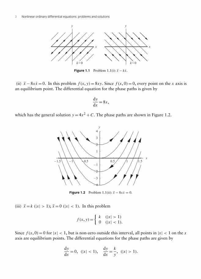
(ii) x−8xx=0. In this problem f (x, y)=8xy. Since f (x, 0)=0, every point on the x axis isan equilibrium point. The differential equation for the phase paths is given by
dydx=8x,
which has the general solution y=4x2+C. The phase paths are shown in Figure 1.2.
– 1.5 – 1 0.5 0.5 1 1.5x
– 4
– 3
– 2
– 1
1
2
3
4y
–
Figure 1.2 Problem 1.1(ii): x − 8xx = 0.
(iii) x= k (|x| > 1); x=0 (|x| < 1). In this problem
f (x, y)=k (|x| > 1)0 (|x| < 1).
Since f (x, 0)=0 for |x| < 1, but is non-zero outside this interval, all points in |x| < 1 on the xaxis are equilibrium points. The differential equations for the phase paths are given by
dydx=0, (|x| < 1),
dydx= ky
, (|x| > 1).

1 : Second-order differential equations in the phase plane 3
– 2 – 1.5 – 1 – 0.5 0.5 1 1.5 2x
1
2
3
y
–3
–2
–1
Figure 1.3 Problem 1.1(iii): x = k (|x| > 1); x = 0 (|x| < 1).
Hence the families of paths are
y=C, (|x| < 1), 12y
2= kx+C, (|x| > 1).
Some paths are shown in Figure 1.3 (see also Section 1.4 in NODE).
(iv) x+3x+2x=0. In this problem f (x, y)=−2x−3y, and there is a single equilibriumpoint, at the origin. This is a linear differential equation which exhibits strong damping (seeSection 1.4) so that the origin is a node. The equation has the characteristic equation
m2+3m+2=0, or (m+1)(m+2)=0.
Hence the parametric equations for the phase paths are
x=Ae−t +Be−2t , y= x= −Ae−t − 2Be−2t .
The node is shown in Figure 1.4.
– 1.5 1.5x
– 1.5
1.5y
Figure 1.4 Problem 1.1(iv): x + 3x + 2x = 0, stable node.

4 Nonlinear ordinary differential equations: problems and solutions
(v) x−4x+40x= 0. In this problem f (x, y)=−40x+4y, and there is just one equilibriumpoint, at the origin. From the results in Section 1.4, this equilibrium point is an unstable spiral.The general solution is
x= e2t [A cos 6t +B sin 6t],from which y can be found. Spiral paths are shown in Figure 1.5.
– 1 1x
– 4
– 2
2
4y
Figure 1.5 Problem 1.1(v): x − 4x + 40x = 0, unstable spiral.
(vi) x+3|x| +2x=0, f (x, y)=−2x−3|y|. There is a single equilibrium point, at the origin.The phase diagram is a combination of a stable node for y >0 and an unstable node for y <0as shown in Figure 1.6. The equilibrium point is unstable.
–1 1x
–1
1y
Figure 1.6 Problem 1.1(vi): x + 3|x| + 2x = 0.
(vii) x+ ksgn (x)+ csgn (x)=0, c > k. Assume that k >0 and x0>0. In this problemf (x, y)=− ksgn (y)− csgn (x), and the system has one equilibrium point, at the origin.

1 : Second-order differential equations in the phase plane 5
By writing
ydydx= 1
2d
dx(y2)
in the equation for the phase paths we obtain
y2=2[−ksgn (y)− csgn (x)]x+C,
where C is a constant. The value of C is assigned separately for each of the four quadrants intowhich the plane is divided by the coordinate axes, using the requirement that the compositephase paths should be continuous across the axes. For the path starting at (x0, 0), its equationin x >0, y <0 is
y2=2(k− c)x+C1.
Therefore C1=2(c− k)x0.Continuity of the path into x <0, y <0 requires
y2=2(k+ c)x+2(c− k)x0.
On the axis y=0, x=−(c− k)x0/(c+ k).The path in the quadrant x <0, y >0 is
y2=2(c − k)x+C2.
By continuity, C2= (c − k)2x0/(c+ k).Finally the path in the quadrant x > 0, y > 0 is
y2=−(c+ k)x+C2.
This path cuts the positive x axis at x= x1= (c− k)2x0/(c+ k)2 as required. Since c > k, itfollows that x1<x0. After n circuits xn= γ nx0 where γ = (c− k)2/(c+ k)2. Since γ <1, thenxn→0. Hence the phase diagram (not shown) is a stable spiral made by matching parabolason the axes.(viii) x+ xsgn (x)=0. The system has a single equilibrium point, at the origin, andf (x, y)=−xsgn (x). The phase paths are given by
y2=−x2+C1, (x >0), y2= x2+C2, (x <0).
The phase diagram is a centre for x >0 joined to a saddle for x <0 as shown in Figure 1.7.

6 Nonlinear ordinary differential equations: problems and solutions
–1 1x
–1
1y
Figure 1.7 Problem 1.1(viii): x + xsgn (x) = 0.
• 1.2 Sketch the phase diagram for the equation x=−x − αx3, considering all values of α.Check the stability of the equilibrium points by the method of Section 1.7.
1.2. x=−x−αx3.Case (i). α >0. The equation has a single equilibrium point, at x=1. The phase paths aregiven by
dydx=−x(1+αx
2)
y,
which is a separable first-order equation. The general solution is given by
∫ydy=−
∫x(1+αx2)dx+C, (i)
so that
12y
2=−12x
2−14x
4+C.
The phase diagram is shown in Figure 1.8 with α=1, and the origin can be seen to be a centre.Case (ii). α <0. There are now three equilibrium points: at x=0 and at x=±1/
√α. The phase
paths are still given by (i), but computed in this case with α=−1 (see Figure 1.9). There is acentre at (0, 0) and saddles at (±1, 0).
This equation is a parameter-dependent system with parameter α as discussed in Section 1.7.As in eqn (1.62), let f (x,α)=−x−αx3. Figure 1.10 shows that in the region above x=0,f (x,α) is positive for all α, which according to Section 1.7 (in NODE) implies that the originis stable. The other equilibrium points are unstable.

1 : Second-order differential equations in the phase plane 7
–2 –1 1 2x
–3
–2
–1
1
2
3
y
Figure 1.8 Problem 1.2: Phase diagram for α=1.
–2 –1 1 2x
–1
1
y
Figure 1.9 Problem 1.2: Phase diagram for α=−1.
–3 –2 –1 1 2 3
1
2x
a
–2
–1
Figure 1.10 Problem 1.2: The diagram shows the boundary x(1−αx2)=0; the shaded regions indicate f (x,α)>0.

8 Nonlinear ordinary differential equations: problems and solutions
• 1.3 A certain dynamical system is governed by the equation x+ x2+ x=0. Show thatthe origin is a centre in the phase plane, and that the open and closed paths are separatedby the path 2y2=1−2x.
1.3. x+ x2+ x=0. The phase paths in the (x, y) plane are given by the differential equation
dydx= −y
2 − xy
.
By putting
ydydx= 1
2d
dx(y2),
the equation can be expressed in the form
d(y2)
dx+2y2=−2x,
which is a linear equation for y2. Hence
y2=Ce−2x − x+ 12 ,
which is the equation for the phase paths.The equation has a single equilibrium point, at the origin. Near the origin for y small,
x+ x≈0 which is the equation for simple harmonic motion (see Example 1.2 in NODE). Thisapproximation indicates that the origin is a centre.
If the constant C <0, then Ce−2x→−∞ as x→∞, which implies that−x+ 12 +Ce−2x must
be zero for a negative value of x. There is also a positive solution for x The paths are closed forC <0 since any path is reflected in the x axis. If C ≥0, then the equation −x+ 1
2 +Ce−2x =0has exactly one solution and this is positive. To see this sketch the line z= x− 1
2 and theexponential curve z=Ce−2x for positive and negative values for C and see where they intersect.The curve bounding the closed paths is the parabola y2=−x+ 1
2 . The phase diagram is shownin Figure 1.11.
• 1.4 Sketch the phase diagrams for the equation x+ ex = a, for a <0, a=0, and a >0.
1.4. x+ ex = a. The phase paths in the (x, y) plane are given by
ydydx= a − ex , (i)

1 : Second-order differential equations in the phase plane 9
–3 –2 –1 1x
–2
–1
1
2y
Figure 1.11 Problem 1.3.
–2 –1 1 2x
–2
–1
1
2y
Figure 1.12 Problem 1.4: a <0.
which has the general solution
12y
2= ax − ex +C. (ii)
Case (a), a < 0. The system has no equilibrium points. From (i), dy/dx is never zero, negativefor y >0 and positive for y <0. Some phase paths are shown in Figure 1.12.Case (b), a=0. The system has no equilibrium points. As in (a), dy/dx is never zero. Somephase paths are shown in Figure 1.13.Case (c), a >0. This equation has one equilibrium point at x= ln a. The potential V(x) (seeSection 1.3) of this conservative system is
V(x)=∫(−a+ ex)dx=−ax+ ex ,
which has the expected stationary value at x= ln a. Since V ′′(ln a)= eln a =a >0, the stationarypoint is a minimum which implies a centre in the phase diagram. Some phase paths are shownin Figure 1.14 for a=2.

10 Nonlinear ordinary differential equations: problems and solutions
–2 –1 1 2x
–2
–1
1
2y
Figure 1.13 Problem 1.4: a=0.
–1 1 2x
–2
–1
1
2y
Figure 1.14 Problem 1.4: a >0.
• 1.5 Sketch the phase diagrams for the equation x− ex = a, for a <0, a=0, and a >0.
1.5. x− ex = a. The differential equation of the phase paths is given by
ydydx= a+ ex ,
which has the general solution
12y
2= ax+ ex +C.
Case (a), a <0. There is a single equilibrium point, at x= ln(−a). The potential V(x) (seeSection 1.3 in NODE) of this conservative system is
V(x)=∫(−a− ex)dx=−ax− ex ,

1 : Second-order differential equations in the phase plane 11
which has the expected stationary value at x= ln(−a). Since
V ′′(ln(−a))=−eln(−a)= a <0,
the stationary point is a maximum, indicating a saddle at x= ln(−a). Some phase paths areshown in Figure 1.15.Case (b), a >0. The equation has no equilibrium points. Some typical phase paths are shownin Figure 1.16.Case (c), a=0. Again the equation has no equilibrium points, and the phase diagram has themain features indicated in Figure 1.16 for the case a >0, that is, phase paths have positive slopefor y >0 and negative slope for y <0.
– –1 1 2x
–2
–1
1
2y
2
Figure 1.15 Problem 1.5: a <0.
–3 –1 1 2x
– 2
– 1
1
2y
Figure 1.16 Problem 1.5: a >0.

12 Nonlinear ordinary differential equations: problems and solutions
• 1.6 The potential energy V(x) of a conservative system is continuous, and is strictlyincreasing for x <−1, zero for |x| ≤1, and strictly decreasing for x >1. Locate theequilibrium points and sketch the phase diagram for the system.
1.6. From Section 1.3, a system with potential V(x) has the governing equation
x=−dV(x)dx
.
Equilibrium points occur where x=0, or where dV(x)/dx=0, which means that all points onthe x axis such that |x| ≤1 are equilibrium points. Also, the phase paths are given by
12y
2=V(x)+C.
Therefore the paths in the interval |x| ≤1 are the straight lines y=C. Since V(x) is strictlyincreasing for x <−1, the paths must resemble the left-hand half of a centre at x=−1. In thesame way the paths for x >1 must be the right-hand half of a centre. A schematic phase diagramis shown in Figure 1.17.
–2 –1 1 2x
1
y
–2 –1 1 2x
–0.2
–0.1
0.1
0.2
v(x)
–1
Figure 1.17 Problem 1.6: This diagram shows some phase paths for the equation with V(x)= x+1, (x <1),V(x)=−x+1, (x >1).
• 1.7 Figure 1.33 (in NODE) shows a pendulum striking an inclined wall. Sketch the phasediagram of this ‘impact oscillator’, for α positive and α negative, when (i) there is no lossof energy at impact, (ii) the magnitude of the velocity is halved on impact.
1.7. Assume the approximate pendulum equation (1.1), namely
θ +ω2θ =0,
and assume that the amplitude of the oscillations does not exceed θ = 12π (thus avoiding any
complications arising from impacts above the point of suspension).
1 : Second-order differential equations in the phase plane 13
u
u ua a
.
u.
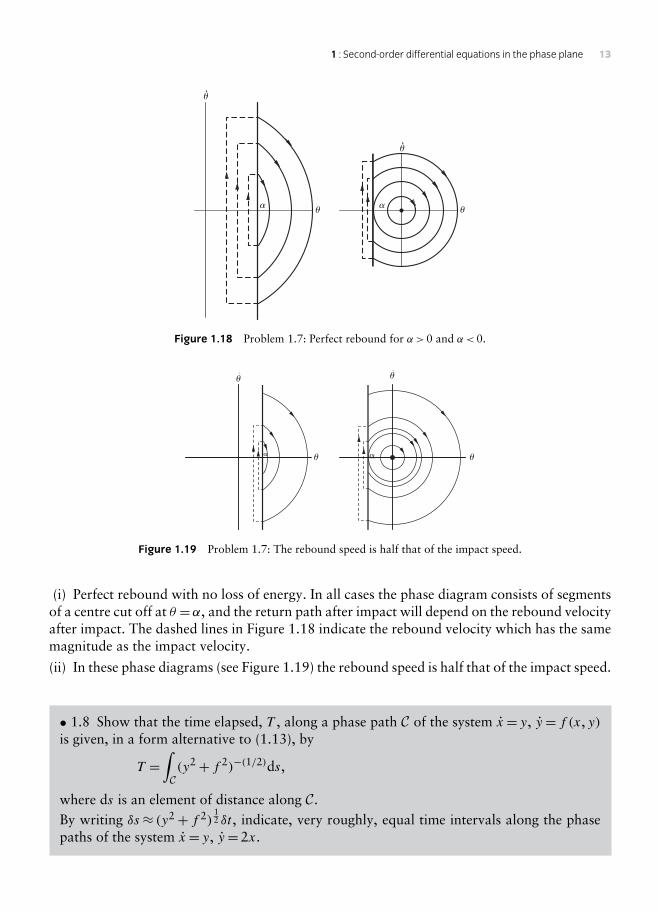
Figure 1.18 Problem 1.7: Perfect rebound for α >0 and α <0.
u u
u.
u.
Figure 1.19 Problem 1.7: The rebound speed is half that of the impact speed.
(i) Perfect rebound with no loss of energy. In all cases the phase diagram consists of segmentsof a centre cut off at θ =α, and the return path after impact will depend on the rebound velocityafter impact. The dashed lines in Figure 1.18 indicate the rebound velocity which has the samemagnitude as the impact velocity.
(ii) In these phase diagrams (see Figure 1.19) the rebound speed is half that of the impact speed.
• 1.8 Show that the time elapsed, T , along a phase path C of the system x= y, y= f (x, y)is given, in a form alternative to (1.13), by
T =∫
C(y2+ f 2)−(1/2)ds,
where ds is an element of distance along C.By writing δs≈ (y2+ f 2)
12 δt , indicate, very roughly, equal time intervals along the phase
paths of the system x= y, y=2x.

14 Nonlinear ordinary differential equations: problems and solutions
–1 1x
1
2y
Figure 1.20 Problem 1.8: The phase path y= (1+2x2)1/2 is shown with equal time steps δt =0.1.
1.8. Let C be a segment of a phase path from A to B, traced out by a representative point Pbetween times TA and tB , and s(t) be the arc length along C measured from A to P . Alongthe path
δs≈[(δx)2+ (δy)2]1/2,
so
δs
δt≈
[(δx
δt
)2
+(δy
δt
)2]1/2
.
In the limit δt→0, the velocity of P is ds/dt given by
dsdt=[x2+ y2]1/2. (i)
The transient time T is given by
T = tB − tA=∫ tB
tA
dt =∫
Cds
ds/dt=
∫C
ds[x2+ y2]1/2 =
∫C(y2+ f 2)−(1/2)ds, (ii)
since x= y and y= f .For the case x= y, y=2x the phase paths consist of the family of hyperbolas y2−2x2=α,
where α is an arbitrary constant. From (i), a small time interval δt corresponds to a step lengthδs along a phase path given approximately by
δs ≈ [x2+ y2]1/2δt = (y2+4x2)1/2δt = (α+6x2)1/2δt .
Given a value of the parameter α, the step lengths for a constant δt are determined by the factor(α+6x2)1/2, and tend to be comparatively shorter when the phase path is closer to the origin.This is illustrated in Figure 1.20 for the branch y= (1− 2x2)1/2.
• 1.9 On the phase diagram for the equation x+ x=0, the phase paths are circles. Use(1.13) in the form δt ≈ δx/y to indicate, roughly, equal time steps along several phasepaths.

1 : Second-order differential equations in the phase plane 15
x
y
Figure 1.21 Problem 1.9.
1.9. The phase paths of the simple harmonic oscillator x+ x=0 are given by dy/dx= − x/y,which has the general solution x2+ y2=C2, C >0. The paths can be represented parametricallyby x=C cos θ , y=C sin θ , where θ is the polar angle. By (1.13), an increment in time isgiven by
δt ≈ δxy= −C sin θδθ
C sin θ=−δθ .
This formula can be integrated to give t =−θ +B. Hence equal time steps are equivalent toequal steps in the polar angle θ . All phase paths are circles centred at the origin and the timetaken between radii subtending the same angle, say α, at the origin as shown in Figure 1.21.
• 1.10 Repeat Problem 1.9 for the equation x+9x=0, in which the phase paths are ellipses.
1.10. The phase paths of x+9x=0 are given by dy/dx=−9x/y, which has the general solu-tion 9x2+ y2=C2, C >0. The paths are concentric ellipses. The paths can be representedparametrically by x= 1
3C cos θ , y=C sin θ , where θ is the polar angle. By (1.13), an incrementin time is given by
δt ≈ δx
y= −(1/3)C sin θδθ
C sin θ=−1
3δθ .
Hence equal time steps are equivalent on all paths to the lengths of segments cut by equal polarangles α as shown in Figure 1.22.

16 Nonlinear ordinary differential equations: problems and solutions
x
y
Figure 1.22 Problem 1.10.
• 1.11 The pendulum equation, x+ω2 sin x=0, can be approximated for moderate ampli-tudes by the equation x+ω2(x− 1
6x3)=0. Sketch the phase diagram for the latter equation,
and explain the differences between it and Figure 1.2 (in NODE).
1.11. For small |x|, the Taylor expansion of sin x is given by
sin x= x − 16x
3+O(x5).
Hence for small |x|, the pendulum equation x+ω2 sin x=0 can be approximated by
x+ω2(x − 1
6x3
)=0.
If x is unrestricted this equation has three equilibrium points, at x=0 and x= ±√6≈±2.45.The pendulum equation has equilibrium points at x= nπ , (n=0, 1, 2, . . .). Obviously, theapproximate equation is not periodic in x, and the equilibrium points at x=±√6 differ con-siderably from those of the pendulum equation. We can put ω=1 without loss since time canalways be rescaled by putting t ′ =ωt . Figure 1.23 shows the phase diagrams for both equationsfor amplitudes up to 2. The solid curves are phase paths of the approximation and the dashed

1 : Second-order differential equations in the phase plane 17
x
–1
1
y
–2 –1 1 2
Figure 1.23 Problem 1.11: The solid curves represent the phase paths of the approximate equation x+ x− 16x
3=0,and the dashed curves show the phase paths of x+ sin x=0.
curves those of the pendulum equation. For |x|<1.5, the phase paths are visually indistin-guishable. The closed phase paths indicate periodic solutions, but the periods will increase withincreasing amplitude.
• 1.12 The displacement, x, of a spring-mounted mass under the action of Coulomb dryfriction is assumed to satisfy
mx+ cx=−F0sgn (x),
where m, c and F0 are positive constants (Section 1.6). The motion starts at t =0, withx= x0>3F0/c and x=0. Subsequently, whenever x=− α, where (2F0/c)− x0<− α <0and x >0, a trigger operates, to increase suddenly the forward velocity so that the kineticenergy increases by a constant amount E. Show that if E>8F 2
0 /c, a periodic motion exists,and show that the largest value of x in the periodic motion is equal to F0/c+E/(4F0).
1.12. The equation for Coulomb dry friction is
mx+ cx=−F0sgn (x)= −F0 x > 0F0 x < 0
.
For x= y <0, the differential equation for the phase paths is given by
mdydx= F0 − cx
y.
Integrating this separable equation, we obtain
12my
2=− 12c (F0 − cx)2+B1= 1
2c (F0 − cx0)2 − 1
2c (F0 − cx)2,

18 Nonlinear ordinary differential equations: problems and solutions
C1
C2
y
C3
xx0x1 –a
Figure 1.24 Problem 1.12:
using the initial conditions x(0)= x0, y(0)=0. This segment of the path is denoted inFigure 1.24 by C1. It meets the x axis again where
F0 − cx=−F0+ cx0, so that x= x1= 2F0
c− x0.
For y >0, phase paths are given by
12my2=− 1
2c(F0+ cx)2+B2. (i)
Denote this segment by C2. It is the continuation into y >0 of C1 from x= x1, y=0. Hence
B2= 12c(F0+ cx1)
2= 12c(3F0 − x0)
2,
so that
x1= 2F0
c− x0.
The condition x1=− x0+ (2F0/c)<−α ensures that the ‘trigger’ operates within the range ofx illustrated.
Denote the segment which meets C1 at x= x0 by C3. From (i), its equation is
12my2 = − 1
2c(F0+ cx)2+B3 = − 1
2c(F0+ cx)2+ 1
2c(F0+ cx0)
2.
At x=−α, the energy on C2 is
E2= 12c[(3F0 − cx0)
2 − (F0 − cα)2],
whilst on C3, the energy is
E3= 12c[(F0+ cx0)
2 − (F0 − cα)2].

1 : Second-order differential equations in the phase plane 19
At x = −α, the energy increases by E. Therefore
E = E3 − E2
= 12c[(F0+ cx0)
2 − (F0 − cα)2] − 12c[(3F0 − cx0)
2 − (F0 − cα)2]
= 12c[(F0+ cx0)
2 − (3F0 − cx0)2]
= 12c[−8F 2
0 +8F0cx0]
A periodic solution occurs if the initial displacement is
x0= E
4F0+ F0
c.
Note that the results are independent of α. For a cycle to be possible, we must have x0>3F0/c.Therefore E and F0 must satisfy the inequality
E
4F0+ F0
c>
3F0
c, or E >
8F 20
c.
• 1.13 In Problem 1.12, suppose that the energy is increased by E at x=−α for both x <0and x >0; that is, there are two injections of energy per cycle. Show that periodic motionis possible if E>6F 2
0 /c, and find the amplitude of the oscillation.
1.13. Refer to the previous problem for the equations of the phase paths in y >0 and y <0.The system experiences an increase in kinetic energy for both y positive and y negative. Theperiodic path consists of four curves whose equations are listed below:
C1: mcy2+ (F0− cx)2= (F0− cx0)2
C2: mcy2+ (F0− cx)2= (F0− cx1)2
C3: mcy2+ (F0+ cx)2= (F0+ cx1)2
C4: mcy2+ (F0+ cx)2= (F0+ cx0)2
The paths, the point (x0, 0) where the paths C1 and C4 meet, and the point (x1, 0) where thepaths C2 and C3 meet are shown in Figure 1.24. At x=−α the energy is increased by E for bothpositive and negative y. The discontinuities at x= − α are shown in Figure 1.25. Therefore, atx= −α,
E= 12c[(F0 − cx1)
2 − (F0+ cα)2 − (F0 − cx0)2+ (F0+ cα)2],
E= 12c[(F0+ cx0)
2 − (F0+ cα)2 − (F0 − cx1)2+ (F0+ cα)2].

20 Nonlinear ordinary differential equations: problems and solutions
x
y
C1C2
C3
C4
x0x1 –a
Figure 1.25 Problem 1.13.
Simplifying these results
E= 12c[−2F0cx1+ c2x2
1 +2F0cx0 − c2x20 ],
E= 12c[2F0cx0+ c2x2
0 − 2F0cx1 − c2x21 ],
Elimination of E gives x1=−x0, and
x0=−x1= E
2F0.
• 1.14 The ‘friction pendulum’ consists of a pendulum attached to a sleeve, which embracesa close-fitting cylinder (Figure 1.34 in NODE). The cylinder is turned at a constant rate>0. The sleeve is subject to Coulomb dry friction through the coupleG=−F0sgn (θ −).Write down the equation of motion, the equilibrium states, and sketch the phase diagram.
1.14. Taking moments about the spindle, the equation of motion is
mga sin θ +F0sgn (θ −)=−ma2θ .
Equilibrium positions of the pendulum occur where θ = θ =0, that is where
mga sin θ − F0sgn (−)=mga sin θ +F0=0,
assuming that >0. Assume also that F0>0. The differential equation is invariant under thechange of variable θ ′ = θ +2nπ so all phase diagrams are periodic with period 2π in θ .
If F0<mga, there are two equilibrium points; at
θ = sin−1(F0
mga
)and π − sin−1
(F0
mga
):
note that in the second case the pendulum bob is above the sleeve.
1 : Second-order differential equations in the phase plane 21
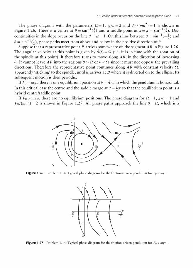
The phase diagram with the parameters =1, g/a=2 and F0/(ma2)=1 is shown in
Figure 1.26. There is a centre at θ = sin−1(12 ) and a saddle point at x=π − sin−1(1
2 ). Dis-continuities in the slope occur on the line θ ==1. On this line between θ = sin−1(−1
2 ) andθ = sin−1(1
2 ), phase paths meet from above and below in the positive direction of θ .Suppose that a representative point P arrives somewhere on the segment AB in Figure 1.26.
The angular velocity at this point is given by θ (t)= (i.e. it is in time with the rotation ofthe spindle at this point). It therefore turns to move along AB, in the direction of increasingθ . It cannot leave AB into the regions θ > or θ < since it must not oppose the prevailingdirections. Therefore the representative point continues along AB with constant velocity ,apparently ‘sticking’ to the spindle, until is arrives at B where it is diverted on to the ellipse. Itssubsequent motion is then periodic.
If F0=mga there is one equilibrium position at θ = 12π , in which the pendulum is horizontal.
In this critical case the centre and the saddle merge at θ = 12π so that the equilibrium point is a
hybrid centre/saddle point.If F0>mga, there are no equilibrium positions. The phase diagram for =1, g/a=1 and
F0/(ma2)=2 is shown in Figure 1.27. All phase paths approach the line θ =, which is a
232
–2
–1
1
2
AB
– 2
.
Ω
Figure 1.26 Problem 1.14: Typical phase diagram for the friction-driven pendulum for F0<mga.
232
–2
–1
1
2.
2 –
Figure 1.27 Problem 1.14: Typical phase diagram for the friction-driven pendulum for F0>mga.

22 Nonlinear ordinary differential equations: problems and solutions
‘singular line’ along which the phase path continues. Whatever initial conditions are impartedto the pendulum, it will ultimately rotate at the same rate as the spindle.
• 1.15 By plotting ‘potential energy’ of the nonlinear conservative system x= x4− x2, con-struct the phase diagram of the system. A particular path has the initial conditions x= 1
2 ,x=0 at t =0. Is the subsequent motion periodic?
1.15. From NODE, (1.29), the potential function for the conservative system defined by
x= x4 − x2
is given by
V(x)=−∫(x4 − x2)dx= 1
3x3 − 1
5x5.
Its graph is shown in the upper diagram in Figure 1.28. The system has three equilibriumpoints: at x=0 and x=±1. The equilibrium point at x=−1 corresponds to a minimum ofthe potential function which generates a centre in the phase diagram, and there is a maximumat x=1 which implies a saddle point. The origin is a point of inflection of V(x). Near theorigin x=− x2 has a cusp in the phase plane. The two phase paths from the origin are given
–1.5 –1 –0.5 0.5 1 1.5x
y
–1 1x
–0.25
0.25
(x)
–1
–0.75
–0.5
–0.25
0.25
0.5
0.75
1
Figure 1.28 Problem 1.15: Potential energy and phase diagram for the conservative system x= x4− x2.

1 : Second-order differential equations in the phase plane 23
by 12y
2=−23x
3 approximately and they only exist for x ≤0. Generally the equations for thephase paths can be found explicitly as
12y
2+V(x)= 12y
2+ 13x
3− 15x
5=C.
A selection of phase paths is shown in the lower diagram of Figure 1.28 including the pathwhich starts at x(0)=− 1
2 , y(0)=0. The closed phase path indicates periodic motion.
• 1.16 The system x+ x=−F0sgn (x), F0>0, has the initial conditions x= x0>0, x=0.Show that the phase path will spiral exactly n times before entering equilibrium (Section 1.6)if (4n−1)F0<x0<(4n+1)F0.
1.16. The system is governed by the equation
x+ x=−F0sgn (x)= −F0 (x > 0)F0 (x < 0.
For y >0, the differential equation of the phase paths is
dydx= −x − F0
y.
Integrating, the solutions can be expressed as
(x+F0)2+ y2=A. (i)
Similarly, for y <0, the phase paths are given by
(x − F0)2+ y2=B. (ii)
For y > 0 the phase paths are semicircles centred at (−F0, 0), and for y <0 they are semicirclescentred at (F0, 0). The equation has a line of equilibrium points for which −1<x <1. Thesemicircle paths are matched as shown in Figure 1.29 (drawn withF0=1), and a path eventuallymeets the x axis between x=−1 and x=1 either from above or below depending on the initialvalue x0. We have to insert a path from (−1, 0) to the origin and a path from (1, 0) to the originto complete the phase diagram.
Let the path which starts at (x0, 0) next cut the x axis at (x1, 0). From (ii) the path is
(x − F0)2+ y2= (x0 − F0)
2, (y < 0).

24 Nonlinear ordinary differential equations: problems and solutions
–3 –2 –1 1 2 3x
– 3
– 2
– 1
1
2
3
y
Figure 1.29 Problem 1.16.
from which it follows that x1=2F0− x0. Assume that 2F0− x0<−F0, that is, x0>3F0 so thatthe path continues. The continuation of the path lies on the semicircle
(x+F0)2+ y2= (x1+F0)
2= (3F0− x0)2, (y > 0).
Assume that it meets the x axis again at x= x2. Hence x2= x0 − 4F0. The spiral will continueif x2>F0 or x0>5F0 and terminate if x0<5F0. Hence just one cycle of the spiral occurs if3F0<x0<5F0.
If the spiral continues then x= x2 becomes the new initial point and a further spiral occurs if
3F0 < x2 < 5F0 or 7F0 < x0 < 9F0.
Continuing this process, a phase path will spiral just n times if
(4n− 1)F0 < x0 < (4n+1)x0.
• 1.17 A pendulum of length a has a bob of mass m which is subject to a horizontal forcemω2a sin θ , where θ is the inclination to the downward vertical. Show that the equation ofmotion is θ =ω2(cos θ − λ) sin θ , where λ= g/(ω2a). Investigate the stability of the equilib-rium states by the method of NODE, Section 1.7 for parameter-dependent systems. Sketchthe phase diagrams for various λ.
1.17. The forces acting on the bob are shown in Figure 1.30. Taking moments about O
mω2a sin θ · a cos θ −mga sin θ =ma2θ ,

1 : Second-order differential equations in the phase plane 25O
a
mg
mv2a sin
Figure 1.30 Problem 1.17.
1 21
2
2
–
–
Figure 1.31 Problem 1.17: The graph of f (θ , λ)=0 where the regions in which f (θ , λ)>0 are shaded.
orθ =ω2(cos θ − λ) sin θ = f (θ , λ),
in the notation of NODE, Section 1.7, where λ/(ω2a). Let ω=1: time can be scaled to eliminateω. The curves in the (θ , λ) given by f (θ , λ)=0 are shown in Figure 1.31 with the regions wheref (θ , λ)>0 are shaded. If λ<1, then the pendulum has four equilibrium points at θ = ± cos−1 λ,θ =0 and θ =π . The diagram is periodic with period 2π in θ so that the equilibrium pointat θ = − π is the same as that at θ =π . Any curves above the shaded regions indicate stableequilibrium points (centres) and any curves below shaded regions indicate unstable equilibriumpoints (saddles). Hence, for λ<1, θ = ± cos−1 λ are stable points, whilst θ =0 and θ =π areboth unstable. The equations of the phase paths can be found by integrating
θdθdθ= sin θ cos θ − λ sin θ .
The general solution isθ2= sin2 θ +2 cos θ +C.
The phase diagram is shown in Figure 1.32 for λ=0.4. As expected from the stabilitydiagram, there are centres at θ =± cos−1 λ and saddles at x=0 and x=π .
If λ ≥ 1, there are two equilibrium point at θ =π (or −π). The phase diagram is shown inFigure 1.33 with λ=2. The origin now becomes a stable centre but θ =π remains a saddle.

26 Nonlinear ordinary differential equations: problems and solutions
–1
1
–
.
Figure 1.32 Problem 1.17: Phase diagram for λ=0.4<1.
–1
1
–
.
Figure 1.33 Problem 1.17: Phase diagram for λ=2>1.
• 1.18 Investigate the stability of the equilibrium points of the parameter-dependent systemx= (x− λ)(x2− λ).
1.18. The equation is
x= (x− λ)(x2− λ)= f (x, λ)
in the notation of NODE, Section 1.7. The system is in equilibrium on the line x= λ and theparabola x2= λ. These boundaries are shown in Figure 1.34 together with the shaded regionsin which f (x, λ)>0.• λ≤0. There is one equilibrium point, an unstable saddle at x= λ.• 0<λ<1. There are three equilibrium points: at x=−√λ (saddle), x= λ (centre) andx=√λ (saddle).
• λ=1. This is a critical case in which f (x, λ) is positive on both sides of x=1. Theequilibrium point is an unstable hybrid centre/saddle.
• λ>1. There are three equilibrium points: at x=−√λ (saddle), x=√λ (centre) and x= λ(saddle).

1 : Second-order differential equations in the phase plane 27
–2 –1 1 2
x
x = x2 =
–2
–1
1
2
Figure 1.34 Problem 1.18.
• 1.19 If a bead slides on a smooth parabolic wire rotating with constant angular velocityω about a vertical axis, then the distance x of the particle from the axis of rotation satisfies(1+ x2)x+ (g−ω2+ x2)x=0. Analyse the motion of the bead in the phase plane.
1.19. The differential equation of the bead is
(1+ x2)x+ (g−ω2+ x2)x=0.
The equation represents the motion of a bead sliding on a rotating parabolic wire with its lowestpoint at the origin. The variable x represents distance from the axis of rotation. Put x= y andg−ω2= λ; then equilibrium points occur where
y=0 and (λ+ y2)x=0.
If λ =0, all points on the x axis of the phase diagram are equilibrium points, and if λ=0 thereis a single equilibrium point, at the origin.
The differential equation of the phase paths is
dydx=− (λ+ y
2)x
(1+ x2)y,
which is a separable first-order equation. Hence, separating the variables and integrating
∫ydyλ+ y2 =−
∫xdx
1+ x2 +C,
or12 ln |λ+ y2| =−1
2 ln(1+ x2)+C,
or(λ+ y2)(1+ x2)=A.

28 Nonlinear ordinary differential equations: problems and solutions
–2 –1 1 2x
y
–2
–1
1
2
Figure 1.35 Problem 1.19: Phase diagram for λ=1.
–2 –1 1 2x
–2
–1
1
2y
Figure 1.36 Problem 1.19: Phase diagram for λ=−1.
• λ>0. The phase diagram for λ=1 is shown in Figure 1.35 which implies that the originis a centre. In this mode, for low angular rates, the bead oscillates about the lowest pointof the parabola.
• λ<0. The phase diagram for λ=−1 is plotted in Figure 1.36 which shows that the originis a saddle. For higher angular rates the origin becomes unstable and the bead will theoret-ically go off to infinity. Note that y= ±1 are phase paths which means, for example, thatthe bead starting from x=0 with velocity y=1 will move outwards at a constant rate.
• λ=1. The phase diagram is shown in Figure 1.37. If the bead is placed at rest at any pointon the wire then it will remain in that position subsequently.

1 : Second-order differential equations in the phase plane 29
–2 –1 1 2x
–2
–1
1
2y
Figure 1.37 Problem 1.19: Phase diagram for λ=0.
• 1.20 A particle is attached to a fixed point O on a smooth horizontal plane by an elasticstring. When unstretched, the length of the string is 2a. The equation of motion of theparticle, which is constrained to move on a straight line through O, is
x=−x+ a sgn (x), |x|>a (when the string is stretched),x=0, |x| ≤ a (when the string is slack),
x being the displacement fromO. Find the equilibrium points and the equations of the phasepaths, and sketch the phase diagram.
1.20. The equation of motion of the particle is
x = −x+ a sgn (x), (|x| > a)x = 0, (|x| ≤ a).
All points in the interval |x| ≤ a, y=0 are equilibrium points. The phase paths as follows.
(i) x >a. The differential equation is
dydx= −x+ a
y,
which has the general solution
y2+ (x − a)2=C1.
These phase paths are semicircles centred at (a, 0).

30 Nonlinear ordinary differential equations: problems and solutions
x
y
a–a
Figure 1.38 Problem 1.20.
(ii) −a≤ x ≤ a. The phase paths are the straight lines y=C2.
(iii) x <−a. The differential equation is
dydx= −x − a
y,
which has the general solutiony2+ (x+ a)2=C3.
These phase paths are semicircles centred at (−a, 0).A sketch of the phase paths is shown in Figure 1.38. All paths are closed which means that
all solutions are periodic.
• 1.21 The equation of motion of a conservative system is x+ g(x)=0, where g(0)=0,and g(x) is strictly increasing for all x, and∫ x
0g(u)du→∞ as x →±∞. (i)
Show that the motion is always periodic.By considering g(x)= xe−x2
, show that if (i) does not hold, the motions are not all necessarilyperiodic.
1.21. The equation for the phase paths is
dydx=−g(x)
y.
The variables separate to give the general solution in the form
12y2=−
∫ x
0g(u)du+C. (i)

1 : Second-order differential equations in the phase plane 31
Write ∫ x
0g(u)du=G(x). (ii)
Then (i) defines two families of paths where C >0;
y=√2C −G(x)1/2 when G(x) < C; (iii)
and the reflection in the x axis;
y=−√2C −G(x)1/2 when G(x) < C. (iv)
Since g(x)<0 when x <0, and g(x)>0 when x >0, then G(x) is strictly increasing to +∞as x→−∞ and x→∞. Also G(x) is continuous and G(0)=0. Therefore, given any value ofC >0, G(x) takes the value C at exactly two values of x, one negative and the other positive.
Consider the family of positive solutions (iii). Take any positive value of the constant C. Atthe two points whereG(x)=C, we have y(x)=0. Between them y(x)>0, and the graph of thepath cuts the x axis at right angles (see Section 1.2). When the corresponding reflected curve(iv) (y <0) is joined to this one, we have a smooth closed curve. By varying the parameter Cthe process generates a family of closed curves nested around the origin (which is therefore acentre), and all motions are periodic.
If g(x)= xe−x2, then G(x)= 1
2 (1− e−x2), which does not go to infinity as x→±∞. The
solutions (iii) and (iv) become
y= ±√2B + 1
2e−x21/2, where B =C− 12 .
If −12 <B <
12 (i.e. if 0<C<1) the above analysis holds; there is a family of closed curves
surrounding the origin. These represent periodic motions. However, ifB > 12 , the corresponding
paths do not meet the x axis, but run from x=−∞ to x=+∞ outside the central region. Theseare not periodic motions.
• 1.22 The wave function u(x, t) satisfies the partial differential equation
∂2u
∂x2 +α∂u
∂x+βu3+ γ ∂u
∂t=0.
where α, β and γ are positive constants. Show that there exist travelling wave solutions ofthe form u(x, t)=U(x − ct) for any c, where U(ζ ) satisfies
d2U
dζ 2 + (α − γ c)dUdζ+βU3=0.
Using Problem 1.21, show that when c=α/γ , all such waves are periodic.

32 Nonlinear ordinary differential equations: problems and solutions
1.22. The wave function u(x, t) satisfies the partial differential equation
∂2u
∂x2 +α∂u
∂x+βu3+ γ ∂u
∂t=0.
Let u(x, t)=U(x− ct) and ζ = x − ct . Then
∂u
∂x= dU
dζ,
∂2u
∂x2 =d2U
dζ 2 ,∂u
∂t=−cdU
dζ,
so that the partial differential equation becomes the ordinary differential equation
d2U
dζ 2 + (α − γ c)dUdζ+βU3=0.
If c=α/γ , the equation becomesd2U
dζ 2 +βU3=0,
which can be compared with the conservative system in Problem 1.21. In this case g(U)=βU3.Obviously g(U)<0 for U <0, g(U)>0 for U >0 and g(0)=0. Also
β
∫ U
0v3dv= β
4U4→∞, as U →±∞.
Therefore by Problem 1.21 these waves are all periodic.
• 1.23 The linear oscillator x+ x+ x=0 is set in motion with initial conditions x=0,x= v, at t =0. After the first and each subsequent cycle the kinetic energy is instanta-neously increased by a constant, E, in such a manner as to increase x. Show that ifE= 1
2v2(1− e4π/
√3), a periodic motion occurs. Find the maximum value of x in a cycle.
1.23. The oscillator has the equation x+ x+ x=0, with initial conditions x(0)=0, x(0)= v.It is easier to solve this equation for x in terms of t rather than to use eqn (1.9) for the phasepaths. The characteristic equation is m2+m+1=0, with roots m= 1
2 (−1±√3i). The general(real) solution is therefore
x(t)= e− 12 t [A cos(1
2
√3t)+ B sin(1
2
√3t)]. (i)
Also we shall require x(t):
x(t)= v√3
e− 12 t [√3 cos(1
2
√3t)− sin(1
2
√3t)]. (ii)

1 : Second-order differential equations in the phase plane 33
x
xv
u
Figure 1.39 Problem 1.23: The limit cycle, with the jump along the y axis.
The first circuit is completed by time t =4π/√
3. x is then equal to u, say, where u isgiven by
u= x(4π/√3)= ve−2π/√
3. (iii)
At this moment(see Figure 1.39) the oscillator receives an impulsive increment E of kineticenergy, of such magnitude as to return the velocity x from its value u to the given initialvelocity v. From (iii)
E= 12v
2 − 12u
2= 12v
2(1− e−4π/√
3). (iv)
The second cycle then duplicates the first, since its initial conditions are physically equivalentto those for the first cycle, and similarly for all the subsequent cycles. The motion is thereforeperiodic, with period T =4π/
√3.
The turning points of x(t) occur where x(t)=0; that is, where tan(√
3/2)=√3 (from (ii)).This has two solutions in the range 0 and 2π . These are
t = 2π
3√
3and t = 4π
3√
3
(by noting that tan−1√
3= 13π ). From (i) the corresponding values of x are
x= ve−π/(3√
3) and x=− ve−2π/(3√
3).
The overall maximum of x(t) is therefore ve−π/(3√
3).
• 1.24 Show how phase paths of Problem 1.23 having arbitrary initial conditions spiral onto a limit cycle. Sketch the phase diagram.

34 Nonlinear ordinary differential equations: problems and solutions
x
yvn–1
vn
Figure 1.40 Problem 1.24: The limit cycle with the jump along the y axis.
1.24. (Refer to Problem 1.23.) The system is the same as that of Problem 1.23, but with theinitial conditions x(0)=0, x(0)= v0>0, where v0 is arbitrary. Suppose the impulsive energyincrement at the end of every cycle is E, an arbitrary positive constant. vn will represent thevalue of x at the end of the nth cycle, following the energy increment delivered at the end ofthat cycle, and it serves as the initial condition for the next cycle (see Figure 1.40).
For the first cycle, starting at x=0, x(0)= v0, we have (as in Problem 1.23)
12v
21 − 1
2v20e−4π/
√3=E,
orv2
1 =2E+ v20e−4π/
√3. (i)
For the second cycle (starting at v1)
v22 =2E+ v2
1e−4π/√
3, (ii)
and so on. For the nth cycle
v2n =2E+ v2
n−1e−4π/√
3. (iii)
By successive substitution we obtain
v2n =2E(1+ e−ρ + · · · + e−(n−1)ρ + v2
0e−nρ), (iv)
in which we have written for brevity ρ=4π/√
3.By using the usual formula for the sum of a geometric series (iv) reduces to
v2n − v2
0 = (1− e−nρ)(
2E1− e−ρ
− v20
)for all n ≥ 1. (v)

1 : Second-order differential equations in the phase plane 35
(A) In the special case when E= 12v
20(1− e−ρ), the right-hand side of (v) is zero, so
v20 = v2
1 = · · · = v2n , which corresponds to the periodic solution in Problem 1.23.
(B) If v20 <2E/(1− e−ρ), the sequence v0, v1, . . . , vn is strictly increasing, and
limn→∞ v2
n =2E
1− e−ρ.
The limit cycle in (A) is approached from inside.
(C) If v20 =2E/(1− e−ρ), the sequence is strictly decreasing and
limn→∞ v2
n =2E
1− eP − ρ ;
so the limit cycle in (A) is approached from the outside.
The more general initial conditions x(0)=X, x(0)=V , where X and V are both arbitrary,correspond to one of the categories (A), (B) or (C); so the same limit (A) is approached.
• 1.25 The kinetic energy, T , and the potential energy, V , of a system with one degree offreedom are given by
T = T0(x)+ xT1(x)+ x2T2(x), V =V(x).Use Lagrange’s equation
ddt
(∂T∂x
)− ∂T∂x=−∂V
∂x
to obtain the equation of motion of the system. Show that the equilibrium points arestationary points of T0(x)−V(x), and that the phase paths are given by the energy equation
T2(x)x2 − T0(x)+V(x)= constant.
1.25. The kinetic and potential energies are given by
T = T0(x)+ xT1(x)+ x2T2(x), V =V(x).
Applying Lagrange’s equation
ddt
(∂T∂x
)− ∂T∂x=−∂V
∂x,
the equation of motion is
ddt(2T2x+ T1)− (T ′2x2+ T ′1x+ T ′0)=−V ′,
or2T2x+ T ′2x2 − T ′0= − V ′. (i)

36 Nonlinear ordinary differential equations: problems and solutions
Equilibrium points, where x= x=0, occur where T ′0−V ′ =0, that is, at the stationary pointsof the energy function T0(x)−V(x). Let y= x. Equation (i) can be expressed in the form
ddx(T2(x)y
2)− T ′0(x)+V ′(x)=0,
which can be integrated to give the phase paths, namely
T2(x)y2 − T0(x)+V(x)=C.
• 1.26 Sketch the phase diagram for the equation x=−f (x+ x), where
f (u)=f0 u ≥ c,f0u/c |u| ≤ c,−f0 u≤ − c
where f0, c are constants, f0>0, and c >0. How does the system behave as c→0?
1.26. The system is governed by the equation x=−f (x+ x), where
f (u)=f0 u > c
f0u/c |u| ≤ c−f0 u < −c
Let y= x. The phase paths are as follows.
• x+ y > c, x=−f0. The equation for the phase paths is
dydx=−f0
y⇒ 1
2y2=−f0x+C1.
The phase paths are parabolas with their axes along the x axis.• |x+ y| ≤ c, x=−f0(x+ x)/c. It is easier to solve the linear equation
cx+ f0x+ f0x=0
parametrically in terms of t . The characteristic equation is
cm2+ f0m+ f0=0.
which has the roots
m1,m2= 12c[−f0 ±√(f 2
0 − 4cf0)].Therefore
x=Aem1t +Bem2t

1 : Second-order differential equations in the phase plane 37
–6 –5 –4 –3 –2 –1 1 2 3x
–1
1
y
x + y = 1
x + y = –1
Figure 1.41 Problem 1.26: The spirals are shown for the parameter values f0=0.25 and c=1. Note that scales onthe axes are not the same in the drawing.
The roots are both real and negative if f0>4c, which means that the phase diagrambetween the lines x+ y= c and x+ y=−c is a stable node. If f0<4c, then the phasediagram is a stable spiral.
• x+ y <−c, x= f0. The phase paths are given by
12y
2= f0x+C2,
which again are parabolas but pointing in the opposite direction.
Figure 1.41 shows a phase diagram for the spiral case. The spiral between the lines x= y=1and x+ y=−1 is linked with the parabolas on either side of the two lines. The total picture isa stable spiral. A similar matching occurs with the stable node.
As c→0, the lines x+ y= c and x+ c=−1 merge and the spiral disappears leaving a centrecreated by the joining of the parabolas.
• 1.27 Sketch the phase diagram for the equation x= u, where
u= −sgn (√
2|x|1/2sgn (x)+ x).(u is an elementary control variable which can switch between +1 and −1. The curve√
2|x|1/2sgn (x)+ y=0 is called the switching curve.)
1.27. The control equation is
x=−sgn [√2|x|1/2sgn (x)+ x].
The equilibrium point satisfies
sgn [√2|x|1/2sgn (x)]=0, or |x|1/2sgn (x)=0,

38 Nonlinear ordinary differential equations: problems and solutions
–6 –4 –2 2 4 6x
–4
–2
2
4y
Figure 1.42 Problem 1.27.
of which x=0 is the only solution. In the phase plane the boundary between the two modes ofthe phase diagram is the switching curve
y=− sgn [√2|x|1/2sgn (x)],
which is two half parabolas which meet at the origin as shown in Figure 1.42. There are distinctfamilies of phase paths on either side of this curve.
• √2|x|1/2sgn (x)+ y >0. The equation is x=−1 so that dy/dx=−1/y and the phase pathsare given by the parabolas y2=−2x+C1
• √2|x|1/2sgn (x)+ y <0. In this case x=1 so that the phase paths are given by y2=2x+C2.
When the parabolic paths reach the switching curve their only exit is along the switching curveinto the equilibrium point at the origin.
• 1.28 The relativistic equation for an oscillator is
ddt
m0x√[1− (x/c)2]
+ kx=0, |x| < c
where m0, c and k are positive constants. Show that the phase paths are given by
m0c2
√[1− (y/c)2] +12kx2= constant.
If y=0 when x= a, show that the period, T , of an oscillation is given by
T = 4c√ε
∫ a
0
[1+ ε(a2 − x2)]dx√(a2 − x2)
√[2+ ε(a2 − x2)] , ε= k
2m0c2 .
The constant ε is small; by expanding the integrand in powers of ε show that
T ≈ π√
2c
(ε−(1/2)+ 3
8ε1/2a2
).

1 : Second-order differential equations in the phase plane 39
1.28. The equation of the oscillator is
ddt
m0x√[1− (x/c)2]
+ kx=0,
which has one equilibrium point at the origin. Also the phase plane is restricted to |x|<c. Lety= x and
f (y)= m0y√[1− (y/c)2] .
Then the equation of the oscillator is
ydf (y)
dy+ kx=0, or yf ′(y)dy
dx+ kx=0.
This is a separable first-order equation with solution
∫yf ′(y)dy=−k
∫dx+C,
which after integration by parts leads to
yf (y)−∫f (y)dy=−1
2kx2+C,
orm0y
2√[1− (y/c)2] −
∫m0ydy√[1− (y/c)2] =−
12kx2+C,
orm0y
2√[1− (y/c)2] +m0c
2√[1− (y/c)2]=−12kx2+C,
so thatm0c
2√[1− (y/c)2] =−
12kx2+C, (i)
as required. A sketch of the phase diagram is shown in Figure 1.43. It can be seen that theorigin is a centre. The particular path through (a, 0) is, from (i),
m0c2
√[1− (y/c)2] =−12kx2+m0c
2+ 12ka2,
or1√[1− (y/c)2] =1+ ε(a2 − x2),

40 Nonlinear ordinary differential equations: problems and solutions
x
y
2
1
–2
–1
Figure 1.43 Problem 1.28: Phase diagram for k=1, c=1 and m0=1.
where ε= k/(2m0c2). Solve this equation for y:
y= dxdt= c√ε√[a2 − x2]√[2+ ε(a2 − x2)]
1+ ε(a2 − x2).
Therefore
T = 4c√ε
∫ a
0
1+ ε(a2 − x2)dx√(a2 − x2)
√[2+ ε(a2 − x2)] ; (ii)
the integral is multiplied by 4 since integration between 0 and a covers a quarter of the period,and the time over each quarter is the same by symmetry.
Expand the integrand in powers of ε for small ε using a Taylor series. Then
1+ ε(a2 − x2)√(a2 − x2)
√[2+ ε(a2 − x2)] ≈ 2−(1/2)[
1√(a2 − x2)
+ 34ε√(a2 − x2)
].
Hence
T ≈ 2√
2c√ε
∫ a
0
[1√
(a2 − x2)+ 3
4ε√(a2 − x2)
]dx
= 2√
2c√ε
[sin−1(x/a)+ 3
8εx√(a2 − x2)+ a2 sin−1(x/a)
]a0
= 2√
2c√ε
(12π + 3
16επa2
)
= π√
2c
(1ε1/2 +
38ε1/2a2
)
as ε→0.

1 : Second-order differential equations in the phase plane 41
• 1.29 A mass m is attached to the mid-point of an elastic string of length 2a and stiffnessλ (see Figure 1.35 in NODE or Figure 1.44). There is no gravity acting, and the tension iszero in the equilibrium position. Obtain the equation of motion for transverse oscillationsand sketch the phase paths.
1.29. Assume that oscillations occur in the direction of x (see Figure 1.44). By symmetry wecan assume that the tensions in the strings on either side ofm are both given by T . The equationof motion for m is
2T sin θ =−mx.
Assuming Hooke’s law,
T = λ× extension= λ[√(x2+ a2)− a].
Therefore
mx=−2kx[√(x2+ a2)− a]√(x2+ a2)
. (i)
There is one expected equilibrium point at x=0. This is a conservative system with potential(see NODE, Section 1.3)
V(x)=2k∫ (
x − ax√(x2+ a2)
)dx= k[x2 − a√(x2+ a2)]. (ii)
The equation of motion (i) can be expressed in the dimensionless form
X′′ =− X√(X2+1)− 1√(X2+1)
after putting x= aX and t =mτ/(2k). The phase diagram in the plane (X,Y =X′) is shown inFigure 1.45. From (ii) the potential energy V has a minimum at x=0 (or X=0) so that theorigin is a centre.
x
mTT
u
Figure 1.44 Problem 1.29.
–2 –1 1 2X
Y
–1
1
Figure 1.45 Problem 1.29: Phase diagram.

42 Nonlinear ordinary differential equations: problems and solutions
• 1.30 The system
x+ x=F(v0 − x)is subject to the friction law
F(u)=
1 u > ε
u/ε −ε < u < ε−1 u < −ε
where u= v0− x is the slip velocity and v0>ε>0. Find explicit equations for the phasepaths in the (x, y= x) plane. Compute a phase diagram for ε=0.2, v0=1 (say). Explainusing the phase diagram that the equilibrium point at (1, 0) is a centre, and that all pathswhich start outside the circle (x − 1)2+ y2= (v0− ε)2 eventually approach this circle.
1.30. The equation of the friction problem is
x+ x=F(v0 − x),where
F(u)=
1 u > ε
u/ε −ε < u < ε−1 u < −ε.
The complete phase diagram is a combination of phase diagrams matched along the linesy= v0+ ε and y= v0 − ε.• y > v0+ ε. In this region F =1. Hence the phase paths satisfy
dydx= − x+1
y,
which has the general solution(x+1)2+ y2=C1.
The phase paths are arcs of circles centred at (−1, 0).• v0 − ε < y < v0+ ε. The differential equation is
x+ x= 1ε(v0 − x), or εx+ x+ εx= v0,
which is an equation of linear damping. The characteristic equation is
εm2+m+ ε=0,
which has the solutions
m1,m2= 12ε[−1±√(1− 4ε2)].

1 : Second-order differential equations in the phase plane 43
–3 –2 –1 1 2 3x
–2
–1
2
y
y = v0 +
y = v0 – 1
Figure 1.46 Problem 1.30: Phase diagram of x+ x=F(v0 − x) for ε=0.2, v0=1.
Since ε is small, the solutions are both real and negative. The general solution is
x=Aem1t +Bem2t + v0
ε.
which is the solution for a stable node centred at (v0/ε, 0).• y < v0 − ε. With F =−1, the phase paths are given by
(x − 1)2+ y2=C2,
which are arcs of circles centred at (1, 0).
Figure 1.46 shows a computed phase diagram for the oscillator with the parameters ε=0.2,v0=1. The equilibrium point at (1, 0) is a centre. The phase paths between y= v0+ ε andy= v0− ε are parts of those of a stable node centred at x= v0/ε=5, y=0. All paths whichstart outside the circle
(x − 1)2+ y2= (v0 − ε)2=0.82,
eventually approach this periodic solution.
• 1.31 The system
x+ x=F(x),where
F(x)=kx+1 x < v00 x= v0−kx − 1 x > v0
,
and k >0, is a possible model for Coulomb dry friction with damping. If k <2, show that theequilibrium point is an unstable spiral. Compute the phase paths for, say, k=0.5, v0=1.Using the phase diagram discuss the motion of the system, and describe the limit cycle.

44 Nonlinear ordinary differential equations: problems and solutions
1.31. The equation for the Coulomb friction is
x+ x=F(x),
where
F(x)=kx+1 x < v00 x= v0−kx − 1 x > v0
For y <v0, the equation of motion is
x − kx+ x=1.
The system has one equilibrium point at x=1 which is unstable, a spiral if k <2 and a node ifk >2. For y >v0, the equation of motion is
x+ kx+ x=−1,
which as part of a phase diagram of a stable spiral or node centred at x=−1. These familiesof paths meet at the line y= v0.
Assume that k <2. For y <v0, the phase paths have zero slope on the line −x+ ky+1=0,which meets the line y= v0 at x= kv0+1. Similarly, the phase paths for y > v0 have zero slopealong the line x+ ky+1=0 which meets the line y= v0 at x=−kv0−1. On the phase diagraminsert a phase path on y= v0 between x=−kv0−1 and x= kv0+1 along which phase pathsmeet pointing in the direction of positive x. In this singular situation the only exit is alongthe line until x= kv0+1 is reached where the path continues for y <v0. See Figure 1.47. Thisparticular path continues as the limit cycle. Paths spiral into the limit cycle from external andinternal points.
The section of phase path on y= v0 corresponds to dry friction in which two surfaces stickfor a time. This occurs in every period of the limit cycle.
–3 –2 –11
2 3x
y
y = v0
–2
–1
1
2
Figure 1.47 Problem 1.31: The phase diagram with k=0.5 and v=1. The thickest curve is the limit cycle.
1 : Second-order differential equations in the phase plane 45
• 1.32 A pendulum with magnetic bob oscillates in a vertical plane over a magnet, whichrepels the bob according to the inverse square law, so that the equation of motion is(Figure 1.36 in NODE)
ma2θ =−mgasinθ +Fh sinφ,
where h>a and F = c/(a2+h2− 2ah cos θ) and c is a constant. Find the equilibrium posi-tions of the bob, and classify them as centres and saddle points according to the parametersof the problem. Describe the motion of the pendulum.
1.32. Take moments about the point of suspension of the pendulum. Then
Fh sinφ −mga sin θ =ma2θ . (i)
where, by the inverse square law,
F = c
a2+h2 − 2ah cos θ, tanφ= a sin θ
h− a cos θ. (ii)
Elimination of f and φ in (i) using (ii) leads to an equation in θ
maθ = ch sin θ(a2+h2 − 2ah cos θ)3/2
−mg sin θ .
There are equilibrium points at θ = nπ , (n=0,±1,±2, . . .) and where
a2+h2 − 2ah cos θ =(ch
mg
)2/3
,
that is where
cos θ = a2+h2 − (ch/mg)2/3
2ah.
This equation has solutions if
−1≤ a2+h2 − (ch/mg)2/3
2ah≤1,
ormg(a − h)3
h≤ c≤ mg(a+h)
3
h. (iii)
If c lies outside this interval then the pendulum does not have an inclined equilibrium position.If it exists let the angle of the inclined equilibrium be θ = θ1 for 0<θ1<π . Obviously θ =−θ1and 2nπ ± θ1 will also be solutions.

46 Nonlinear ordinary differential equations: problems and solutions
This is a conservative system with potential V(θ) (see Section 1.3) such that
V ′(θ)=− ch sin θma(a2+h2 − 2ah cos θ)3/2
+ g sin θa
.
The nature of the stationary points can be determined by the sign of the second derivative ateach point. Thus
V ′′(θ)=− ch cos θma(a2+h2 − 2ah cos θ)3/2
+ 3ch2 sin2 θ
m(a2+h2 − 2ah cos θ)5/2+ g cos θ
a.
• θ = nπ (n even).
V ′′(nπ)=− ch
ma(h− a)3 +g
a.
It follows that θ = nπ is a centre if c <mg(h− a)3/h and a saddle if c >mg(h− a)3/h.• θ = nπ (n odd).
V ′′(nπ)= ch
ma(h+ a)3 −g
a.
Therefore θ = nπ is a centre if c >mg(h+ a)3/h and a saddle if c <mg(h+ a)3/h.• θ = θ1 subject to mg(a − h)3≤ ch≤mg(a+h)3.
V ′′(θ1) = − ch cos θ1ma(a2+h2 − 2ah cos θ1)3/2
+ 3ch2 sin2 θ1
m(a2+h2 − 2ah cos θ1)5/2+ g cos θ1
a
=(mgch
)−(5/3) ch2 sin2 θ1
m
> 0.
Note that V(−θ1) is also positive Therefore, if they exist, all inclined equilibrium points arecentres.
Suppose that the parameters a, h and m are fixed, and that c can be increased from zero. Thebehaviour of the bob is as follows:
• 0<c<mg(a−h)3/h. There are two equilibrium positions: the bob vertically below thesuspension point which is a stable centre, or the bob above which is an unstable saddle,
• c takes the intermediate values defined by (iii). Both the highest and lowest points becomesa saddles. The inclined equilibrium points are centres.
• c >mg(a+h)3/h. The lowest point remains a saddle but the highest point switches backto a saddle.
1 : Second-order differential equations in the phase plane 47
• 1.33 A pendulum with equation x+ sin x=0 oscillates with amplitude a. Show that itsperiod, T , is equal to 4K(β), where β = sin2 1
2a and
K(β)=∫ 1
2π
0
dφ√(1− β sin2 φ)
.
The function K(β)has the power series representation
K(β)= 12π
[1+
(12
)2
β +(
1.32.4
)2
β2+ · · ·]
, |β| < 1.
Deduce that, for small amplitudes,
T =2π(
1+ 116a2+ 11
3072a4
)+O(a6).
1.33. The pendulum equation x+ sin x=0 can be integrated once to give the equation of thephase paths in the form
12 x
2 − cos x=C=− cos a, (i)
using the condition that x= a when x=0. The origin is a centre about which the paths aresymmetric in both the x and y= x axes. Without loss of generality assume that t =0 initially.The pendulum completes the first cycle when x=2π . From (i) the quarter period is
K =∫ K
0dt = 1√
2
∫ a
0
dx√(cos x − cos a)
= 12
∫ a
0
dx√(sin2(1/2)a − sin2(1/2)x)
.
Now apply the substitution sin 12x= sin 1
2a sinφ so that the limits are replaced by φ=0 andφ= 1
2π . Since
12 cos 1
2xdxdφ= sin 1
2a cosφ,
then
K(β)=∫ 1
2π
0
dφ√(1− β sin2 φ)
.
For small β, expand the integrand in powers of β using the binomial expansion so that
K(β) =∫ ( 1
2 )π
0
(1+ 1
2β sin2 φ+ 3
8β2 sin4 φ+ · · ·
)dφ
= 12π + 1
8πβ + 9
128β2π + · · ·

48 Nonlinear ordinary differential equations: problems and solutions
Now expand β in powers of a:
β = sin2 12a= 1
2a − 1
48a3+O(a5).
Finally
T = 4K(β)
= 2π[1+ 1
4
(14a2 − 1
48a4
)+ 9
1024a4+O(a6)
]
= 2π(
1+ 116a2+ 11
3072a4
)+O(a6).
as a→0.
• 1.34 Repeat Problem 1.33 with the equation x+ x− εx3=0 (ε >0), and show that
T = 4√
2√(2− εa2)
K(β), β = εa2
2− εa2 ,
and that
T =2π(
1+ 38εa2+ 57
256ε2a4
)+O(ε3a6)
as εa2 → 0.
1.34. The damped equation x+ x − εx3=0 has phase paths given by
12 x
2= 14εx
4 − 12x
2+C= 14εx
4 − 12x
2 − 14εa
4+ 12a
2,
= 12 (x
2 − a2)(εx2+ εa2 − 2)
assuming that x= a when x=0. The equation has equilibrium points at x=0 and x=±1/√ε.
Oscillations about the origin (which is a centre) occur if a√ε <1. In this case the period T is
given by
T = 4√
2∫ a
0
dx√(a2x2)
√(2− εa2 − εx2)
= 4√
2∫ (1/2)π
0
dφ√(2− εa2 − εa2 sin2 φ)
(substituting x= sinφ)
= 4√
2√(2− εa2)
K(β)

1 : Second-order differential equations in the phase plane 49
where β = εa2/(2− εa2) and
K(β)=∫ (1/2)π
0
dφ√(1− β sin2 φ)
.
From the previous problem, with µ= εa2,
T = 2π√
2√(2− µ)
[1+ µ
4(2− µ) +9µ2
64(2− µ)2 +O(µ3)
]
= 2π√
2√(2− µ)
[1+ 1
8µ
(1+ 1
2µ
)+ 9µ2
256+O(µ3)
]
= 2π
(1+ µ
4+ 3µ2
32
)(1+ µ
8+ 25µ2
256
)+O(µ3)
= 2π
(1+ 3µ
8+ 57µ2
256
)+O(µ3)
as µ→0.
• 1.35 Show that the equations of the form x+ g(x)x2+h(x)=0 are effectively conserva-tive. (Find a transformation of x which puts the equations into the usual conservative form.Compare with NODE, eqn (1.59).)
1.35. The significant feature of the equation
x+ g(x)x2+h(x)=0 (i)
is the x2 term. Let z= f (x), where f (x) is twice differentiable and it is assumed that z= f (x)can be uniquely inverted into x= f−1(z). Differentiating
z= f ′(x)x, z= f ′(x)x+ f ′′(x)x2.
Therefore
x= z
f ′(x), x= z
f ′(x)− f ′′(x)x2
f ′(x)= z
f ′(x)− f ′′(x)z2
f ′(x)3.
Substitution of these derivatives into (i) results in
z− f ′′(x)f ′(x)2
z2+ g(x)
f ′(x)z2+ f ′(x)h(x)=0.

50 Nonlinear ordinary differential equations: problems and solutions
The z2 can be eliminated by choosing f ′(x) so that
f ′′(x)f ′(x)
= g(x).
Aside from a constant we can put
f ′(x)= exp[∫ x
g(u)du]
,
and a further integration leads to
f (x)=∫
exp[∫ x
g(u)du]
dx.
In terms of z the equation becomes
z+p(z)=0,
where p(z)= f ′(f−1(z))h(f−1(z)). Obviously this equation is conservative of the form (1.23).
• 1.36 Sketch the phase diagrams for the following.
(i) x= y, y=0, (ii) x= y, y=1, (iii) x= y, y= y.
1.36. (i) x= y, y=0. All points on the x axis are equilibrium points. The solutions are x= t +Aand y=B. The phase paths are lines parallel to the x axis (see Figure 1.48).(ii) x= y, y=1. There are no equilibrium points. The equation for phase paths is
dydx= 1y
,
whose general solution is given by y2=2x+C. The phase paths are congruent parabolas withthe x axis as the common axis (see Figure 1.48).(iii) x= y, y= y. All points on the x axis are equilibrium points. The phase paths are given by
dydx=1 ⇒ y= x+C,
which are parallel inclined straight lines (see Figure 1.49). All equilibrium points are unstable.

1 : Second-order differential equations in the phase plane 51
x
y
1 2 3x
1
2y
–3 –2 –1
–2
–1
Figure 1.48 Problem 1.36: The phase diagrams for (i) and (ii).
x
y
Figure 1.49 Problem 1.36: The phase diagram (iii).
• 1.37 Show that the phase plane for the equation
x − εxx+ x=0, ε > 0
has a centre at the origin, by finding the equation of the phase paths.
1.37. The differential equation for the phase paths of
x − εxx+ x=0,
is
ydydx− εxy+ x=0.
This is a separable equation having the general solution
ε
∫xdx=
∫ydy
y − ε−1 +C=∫ (
1+ ε−1
y − ε−1
)dy+C,
or
12εx
2= y+ ε−1 ln |y − ε−1| +C, (i)
where C is a constant. Note that there is a singular solution y= ε−1. The system has a singleequilibrium point, at the origin.

52 Nonlinear ordinary differential equations: problems and solutions
To establish a centre it is sufficient to show that all paths in some neighbourhood of the pointare closed, so we may restrict consideration to the region y < ε−1. On this range put
F(y)=−y − ε−1 ln |y − ε−1| =−y − ε−1 ln(ε−1 − y). (ii)
Then from (i) and (ii) we can express the paths as the union of two families of curves:
x=√2ε−(1/2)C − F(y)1/2 ≥ 0, (iii)
andx=−√2ε−(1/2)C − F(y)1/2, (iv)
(wherever C−F(y) is non-negative). The curves in (iv) are the reflections in the y axis of thosein (iii), and the families join up smoothly across this axis.
Evidently, for y < ε−1,F(0)=−ε−1 ln(ε−1) (v)
and
F ′(y)= y
ε−1 − y =< 0 if y < 0zero if y=0> 0 if y > 0
. (vi)
Therefore F(y) has a minimum at y=0. Also F(y) is strictly increasing in both directions awayfrom y=0 and (from (ii)) F(y)→+∞ as y→−∞ and as y→ ε−1 from below.
Consider eqn (iii), using (v) and (vi). If
−ε−1 ln(ε−1) < C <∞ (vii)
there are exactly two values in the range−∞<y <ε−1 at which the factor C−F(y), and hencex, becomes zero, and between these values x >0. The corresponding reflected path segmentgiven by (iv) completes a closed path, having parameter C. A representative phase diagram isgiven in Figure 1.50. The unclosed paths correspond to values of y > ε−1: their boundary is thesingular solution mentioned above.
• 1.38 Show that the equation x+ x+ εx3=0 (ε >0) with x(0)= a, x(0)=0 has phasepaths given by
x2+ x2+ 12εx
4= (1+ 12εa
2)a2.
Show that the origin is a centre. Are all phase paths closed, and hence all solutions periodic?
1.38. The differential equation of the phase paths of
x+ x+ εx3=0, (ε > 0)
1 : Second-order differential equations in the phase plane 53
–1 1x
–1
1
y
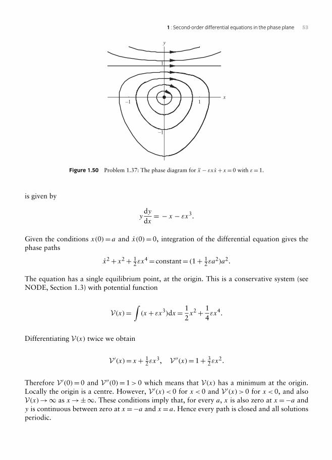
Figure 1.50 Problem 1.37: The phase diagram for x − εxx+ x=0 with ε=1.
is given by
ydydx= − x − εx3.
Given the conditions x(0)= a and x(0)=0, integration of the differential equation gives thephase paths
x2+ x2+ 12εx
4= constant= (1+ 12εa
2)a2.
The equation has a single equilibrium point, at the origin. This is a conservative system (seeNODE, Section 1.3) with potential function
V(x)=∫(x+ εx3)dx= 1
2x2+ 1
4εx4.
Differentiating V(x) twice we obtain
V ′(x)= x+ 12εx
3, V ′′(x)=1+ 32εx
2.
Therefore V ′(0)=0 and V ′′(0)=1>0 which means that V(x) has a minimum at the origin.Locally the origin is a centre. However, V ′(x)<0 for x <0 and V ′(x)>0 for x <0, and alsoV(x)→∞ as x→±∞. These conditions imply that, for every a, x is also zero at x=−a andy is continuous between zero at x=−a and x= a. Hence every path is closed and all solutionsperiodic.

54 Nonlinear ordinary differential equations: problems and solutions
• 1.39 Locate the equilibrium points of the equation
x+ λ+ x3 − x=0.
in the x, λ plane. Show that the phase paths are given by12 x
2+ λx+ 14λx
4 − 12x
2= constant.
Investigate the stability of the equilibrium points.
1.39. Consider the parameter-dependent system
x+ λ+ x3 − x=0.
Using the notation of Section 1.7 (in NODE), let f (x, λ)= x−x3−λ. Equilibrium points occurwhere f (x, λ)=0 which is shown as the curve in Figure 1.51. The function f (x, λ) is positive inthe shaded region. Points on the curve λ= x−x3 above the shaded areas are stable and all otherpoints are unstable. Treating λ as a function of x, x − x3 has stationary points at x=±1/
√3
where λ=±2/√
3 as indicated in Figure 1.51. Therefore if −2/√
3<λ<2/√
3 the equationhas three equilibrium points; if λ= ± 2/
√3 the equation has two; for all other values of λ the
equation has one equilibrium point. The phase paths satisfy the differential equation
ydydx=−x3+ x − λ,
where y= x. Integrating, the phase paths are given by
12y
2+ λx+ 14x
4 − 12x
2= constant.
x
1
–1
f (x, ) > 0
1
–1
Figure 1.51 Problem 1.39: Graph showing equilibrium points on λ= x − x3.
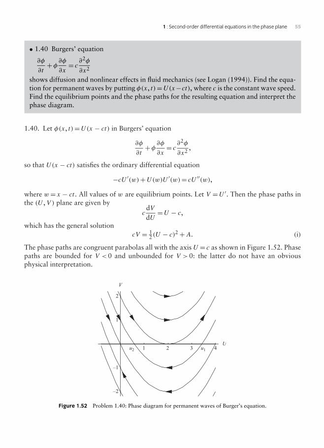
1 : Second-order differential equations in the phase plane 55
• 1.40 Burgers’ equation
∂φ
∂t+φ ∂φ
∂x= c∂
2φ
∂x2
shows diffusion and nonlinear effects in fluid mechanics (see Logan (1994)). Find the equa-tion for permanent waves by putting φ(x, t)=U(x−ct), where c is the constant wave speed.Find the equilibrium points and the phase paths for the resulting equation and interpret thephase diagram.
1.40. Let φ(x, t)=U(x − ct) in Burgers’ equation
∂φ
∂t+φ ∂φ
∂x= c∂
2φ
∂x2 ,
so that U(x − ct) satisfies the ordinary differential equation
−cU ′(w)+U(w)U ′(w)= cU ′′(w),where w= x − ct . All values of w are equilibrium points. Let V =U ′. Then the phase paths inthe (U ,V ) plane are given by
cdVdU
=U − c,which has the general solution
cV = 12 (U − c)2+A. (i)
The phase paths are congruent parabolas all with the axis U = c as shown in Figure 1.52. Phasepaths are bounded for V <0 and unbounded for V >0: the latter do not have an obviousphysical interpretation.
1 2 3 4U
V
u1u2
–2
–1
1
2
Figure 1.52 Problem 1.40: Phase diagram for permanent waves of Burger’s equation.

56 Nonlinear ordinary differential equations: problems and solutions
w
Uu1
u2
Figure 1.53 Problem 1.40: A permanent waveform of Burgers’ equation.
Burgers’ equation describes a convection-diffusion process, and a solution U(x − ct) is theshape of a wavefront. ForU ′ < 0, the wavefront starts atU = u1, say, and terminates atU = u2.We can obtain an explicit form for the wave if we assume that U→ u1 as w→∞, and U→ u2as w→−∞, and U ′ → 0 in both cases, with u2<u1. Hence from (i),
A=−12 (u1 − c)2=−1
2 (u2 − c)2,
so that c= 12 (u1+ u2) and A=− 1
8 (u1 − u2)2. Hence (i) becomes
−cU = (U − u1)(U − u2).
This is a separable equation with solution
w= u1+ u2
u2 − u1
∫ (dU
U − u1+ dUu2 − U
)= u1+ u2
u2 − u1ln
[u2 − UU − u1
].
Solving for U we obtain
U(x − ct)= u1+ u2 − u1
1+ exp[(u2 − u1)(x − ct)/(u1+ u2)] .
The shape of the waveform is indicated in Figure 1.53.
• 1.41 A uniform rod of mass m and length L is smoothly pivoted at one end and held ina vertical position of equilibrium by two unstretched horizontal springs, each of stiffnessk, attached to the other end as shown in Figure 1.37 (in NODE) or Figure 1.54. The rodis free to oscillate in a vertical plane through the springs and the rod. Find the potentialenergy V(θ) of the system when the rod is inclined at an angle θ to the upward vertical. Forsmall θ confirm that
V(θ) ≈ (kL− 14mg)Lθ
2,
Sketch the phase diagram for small |θ |, and discuss the stability of this inverted pendulum.

1 : Second-order differential equations in the phase plane 57
(L sin , LT cos )
L
Figure 1.54 Problem 1.41: Inverted pendulum inclined at angle θ .
1.41. Let the distance between the supports be 2a, and let the origin be at the hinge withhorizontal and vertical axes. The supports have coordinates (a,L) and (−a,L). The potentialenergy includes contributions from the height of the bob and the springs. We assume that thesprings obey Hooke’s law which states that
potential energy= 12 (stiffness)× (extension)2.
Therefore the potential energy is
V(θ) = 12mgL cos θ − 1
2mgL+ 12k√[(a − L sin θ)2+ (L− L cos θ)2] − a2
+ 12k√[(a+L sin θ)2+ (L− L cos θ)2] − a2
defined so that V(0)=0.For |θ | small, use the approximations sin θ ≈ θ and cos θ ≈1− 1
2θ2. Then
V(θ) ≈ −14mgLθ
2+ 12k√[(a − Lθ)2+Lθ2] − a2
+ 12k√[(a+Lθ)2+Lθ2] − a2,
= −14mgLθ2+ 1
2k
a
(1− 2Lθ
a+ 2L2θ2
a2
)1/2
− a
2
+ 12k
a
(1+ 2Lθ
a+ 2L2θ2
a2
)1/2
− a
2
≈ −14mgLθ2+ kL2θ2
as required.

58 Nonlinear ordinary differential equations: problems and solutions
The potential energy is a minimum if Lk > 14mg (springs with strong stiffness) which means
that the bob oscillates about equilibrium in a centre. If Lk < 14mg (weak stiffness) then the
potential energy has a maximum (saddle point in the phase diagram) and the bob is in unstableequilibrium. The phase diagrams are typically those shown in Figure 1.12 in NODE.
• 1.42 Two stars, each with gravitational mass µ, are orbiting each other under theirmutual gravitational forces in such a way that their orbits are circles of radius a. A satelliteof relatively negligible mass is moving on a straight line through the mass centre G suchthat the line is perpendicular to the plane of the mutual orbits of this binary system. Explainwhy the satellite will continue to move on this line. If z is the displacement of the satellitefrom G, show that
z=− 2µz(a2+ z2)3/2
.
Obtain the equations of the phase paths. What type of equilibrium point is z=0?
1.42. Let F be the gravitational force on the satellite S (mass m) due to one of the stars asshown in Figure 1.55. By the inverse square law
F = mµ
z2+ a2 .
Resolution in the direction GS gives
−2µ cos θz2+ a2 =mz,
or2µz
(z2+ a2)32
= z. (i)
Transverse forces balance which means that the satellite will continue to move along the z axis.
FF
G
z
a a
S
Figure 1.55 Problem 1.42.

1 : Second-order differential equations in the phase plane 59
The satellite has a single equilibrium point, at G. The phase paths are given by
12z2= − 2µ
∫zdz
(z2+ a2)3/2= 2µ(z2+ a2)1/2
+C.
From (i), near the origin
z ≈ −3µza3 ,
which indicates that the equilibrium point is a centre.
• 1.43 A long wire is bent into the shape of a smooth curve with equation z= f (x) in afixed vertical (x, z) plane (assume that f ′(x) and f ′′(x) are continuous). A bead of mass mcan slide on the wire: assume friction is negligible. Find the kinetic and potential energiesof the bead, and write down the equation of the phase paths. Explain why the method ofSection 1.3 concerning the phase diagrams for stationary values of the potential energy stillholds.
1.43. The bead and wire are shown in Figure 1.56. The components of the velocity of the beadare given by (x, z= f ′(x)x). The kinetic and potential energies are
T = 12m(x2+ z2)= 1
2m(1+ f ′(x)2)y2, V =mgy=mgf (x),
where y= x in the phase plane.Equilibrium points occur where V ′(x)=0, that is, at the stationary points of the curve
z= f (x). Suppose that a stationary value occurs at x= x1, so that f ′(x1)=0. At the equi-librium point let C1=mgf (x1). Suppose that x= x1 is a minimum. Then for C > C1 butsufficiently close to C1, the phase path will be
y2= 2[C −mgf (x)]m[1+ f ′(x)2] ,
x
x
z
z = f (x) y
m
·
·
Figure 1.56 Problem 1.43.

60 Nonlinear ordinary differential equations: problems and solutions
and y will be zero where x satisfies C1=mgf (x). As in Figure 1.12 (in NODE), the equilibriumpoint will be a centre. Similar arguments apply to the other types of stationary values.
• 1.44 In the previous problem suppose that friction between the bead and the wire isincluded. Assume linear damping in which motion is opposed by a frictional force pro-portional (factor k) to the velocity. Show that the equation of motion of the bead isgiven by
m(1+ f ′(x)2)x+mf ′′(x)x2+ kx(1+ f ′(x)2)+mgf ′(x)=0,
where m is its mass.Suppose that the wire has the parabolic shape given by z= x2 and that dimensions are
chosen so that k=m and g=1. Compute the phase diagram in the neighbourhood of theorigin, and explain general features of the diagram near and further away from the origin.(Further theory and experimental work on motion on tracks can be found in the book byVirgin (2000).)
1.44. Let R be the normal reaction of the bead on the wire and let F be the frictionalforce opposing the motion as shown in Figure 1.57. The horizontal and vertical equations ofmotion are
−R sin θ − F cos θ =mx, (i)
R cos θ −mg − F sin θ =mz, (ii)
where θ is the inclination of the tangent of the curve at the bead. Since z= f (x), then z= f ′(x)xand z= f ′′(x)x2+ f ′(x)x. Eliminate R between (i) and (ii):
−[mg+ kxf ′(x)] sin θ − F(sin2 θ + cos2 θ)=m[f ′′(x)x2+ f ′′(x)x]+mx cos θ , (iii)
where sin θ = f ′(x)/√[1+ f ′(x)2] and cos θ =1/√[1+ f ′(x)2]. The frictional force F is
proportional to the velocity and opposes the motion: therefore
F = − k(x cos θ + z sin θ)= − x√[1+ f ′(x)2].
x
z
m x.
y.
mgF
u
R
z = f (x)
Figure 1.57 Problem 1.44.

1 : Second-order differential equations in the phase plane 61
–2 –1 1 2x
–1
1
y
Figure 1.58 Problem 1.44: Phase diagram for (1+4x2)x+2x2+ x(1+4x2)=−2x.
Finally, the equation of motion is
m(1+ f ′(x)2)x+mf ′′(x)x2+ kx(1+ f ′(x)2)+mgf ′(x)=0.
If f (x)= x2, m= k and g=1, then the equation of motion becomes
(1+4x2)x+2x2+ x(1+4x2)+2x=0.
The phase diagram is shown in Figure 1.58 in the region −2≤ x ≤2, −1.5≤ y ≤1.5. For smallx and y,
x+ x+2x ≈ 0,
neglecting the x2 and y2 terms. Locally the phase diagram is a stable spiral, although furtheraway from the origin the spiral shape is distorted by the nonlinear terms.

This page intentionally left blank
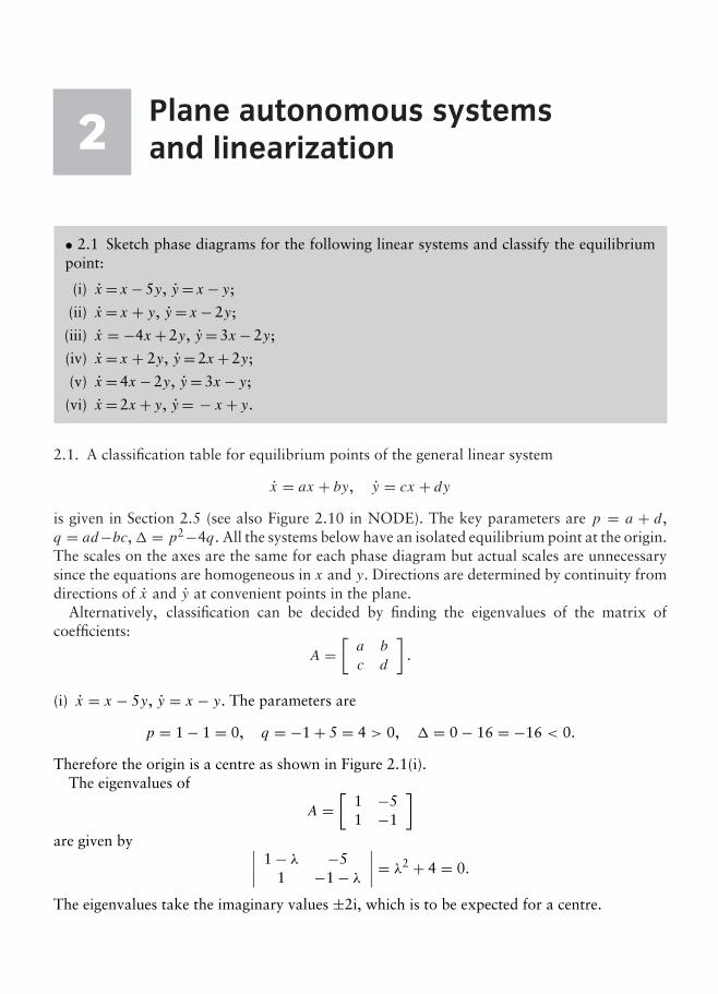
2 Plane autonomous systemsand linearization
• 2.1 Sketch phase diagrams for the following linear systems and classify the equilibriumpoint:
(i) x= x−5y, y= x− y;
(ii) x= x + y, y= x−2y;
(iii) x = −4x+2y, y=3x−2y;
(iv) x= x + 2y, y=2x+2y;
(v) x=4x−2y, y=3x− y;
(vi) x=2x+ y, y= − x+ y.
2.1. A classification table for equilibrium points of the general linear system
x = ax + by, y = cx + dyis given in Section 2.5 (see also Figure 2.10 in NODE). The key parameters are p = a + d,q = ad−bc, = p2−4q. All the systems below have an isolated equilibrium point at the origin.The scales on the axes are the same for each phase diagram but actual scales are unnecessarysince the equations are homogeneous in x and y. Directions are determined by continuity fromdirections of x and y at convenient points in the plane.
Alternatively, classification can be decided by finding the eigenvalues of the matrix ofcoefficients:
A =[a b
c d
].
(i) x = x − 5y, y = x − y. The parameters are
p = 1− 1 = 0, q = −1+ 5 = 4 > 0, = 0− 16 = −16 < 0.
Therefore the origin is a centre as shown in Figure 2.1(i).The eigenvalues of
A =[
1 −51 −1
]are given by ∣∣∣∣ 1− λ −5
1 −1− λ∣∣∣∣ = λ2 + 4 = 0.
The eigenvalues take the imaginary values ±2i, which is to be expected for a centre.

64 Nonlinear ordinary differential equations: problems and solutions
x
y
x
y
Figure 2.1 Problem 2.1(i): x = x − 5y, y = x − y, centre; (ii) x = x + y, y = x − 2y, saddle.
(ii) x = x + y, y = x − 2y. The parameters are
p = 1− 2 = −1 < 0, q = −2− 1 = −3 < 0, = 1+ 12 = 13 > 0.
Therefore the origin is a saddle. Its asymptotes can be found by putting y = mx into theequation for the phase paths which is
dydx= x − 2y
x + y .
The result is
m = 1− 2m1+m , so that m2 + 3m− 1 = 0.
Therefore the slopes of the asymptotes are
m1,m2 = 12 (−3±√13).
The asymptotes and some phase paths are shown in Figure 2.1(ii).
(iii) x = −4x + 2y, y = 3x − 2y. The parameters are
p = −4− 2 = −6 < 0, q = 8− 6 = 2 > 0, = 36− 8 = 28 > 0.
Therefore the origin is a stable node. The radial straight paths are given by y = mx where
m = 3− 2m−4+ 2m
or 2m2 − 2m− 3 = 0.
Hence the radial paths are
y = m1x, y = m2x, where m1,m2 = 12(1±√7).
The radial paths and some phase paths are shown in Figure 2.2(iii).
(iv) x = x + 2y, y = 2x + 2y. The parameters are
p = 1+ 2 = 3 > 0, q = 2− 4 = −2 < 0, = 9+ 8 = 17 > 0.
The origin is a saddle. The slopes of the asymptotes are
m1,m2 = 12 (1±
√17).

2 : Plane autonomous systems and linearization 65
x
y
x
y
Figure 2.2 Problem 2.1(iii) :x = −4x + 2y, y = 3x − 2y, stable node; (iv) x = x + 2y, y = 2x + 2y, saddle.
See Figure 2.2(iv)
(v) x = 4x − 2y, y = 3x − y. The parameters are
p = 4− 1 = 3 > 0, q = −4+ 6 = 2 > 0, = 9− 8 = 1 > 0.
Therefore the origin is an unstable node. The radial paths have slopes m1 = 12 and m2 = 3 and
equationsy = 1
2x, y = 3x.
The phase diagram is shown in Figure 2.3(v).
x
y
x
y
Figure 2.3 Problem 2.1(v): x = 4x − 2y, y = 3x − y, unstable node; (vi) x = 2x + y, y = −x + y, unstable spiral.
(vi) x = 2x + y, y = −x + y. The parameters are
p = 2+ 1 = 3 > 0, q = 2+ 1 = 3 > 0, = 9− 12 = −3 < 0.
The origin is an unstable spiral. Some phase paths are shown in Figure 2.3(vi).
• 2.2 Some of the following systems either generate a single eigenvalue, or a zero eigenvalue,or in other ways vary the types illustrated in Section 2.5. Sketch their phase diagrams
(i) x = 3x − y, y = x + y;
(ii) x = x − y, y = 2x − 2y;
(iii) x = x, y = 2x − 3y;

66 Nonlinear ordinary differential equations: problems and solutions
(iv) x = x, y = x + 3y;
(v) x = −y, y = 2x − 4y;
(vi) x = x, y = y;
(vii) x = 0, y = x.
2.2. Note that the scales on both axes are the same.
(i) x = 3x − y, y = x + y. Using the classification table (See Section 2.5)
p = 3+ 1 = 4 > 0, q = 3+ 1 = 4 > 0, = 16− 16 = 0.
Hence the origin is an unstable degenerate node with a repeated eigenvalue of m = 1. Thestraight line y = x contains radial paths (Figure 2.4).
x
y
x
yy
Figure 2.4 Problem 2.2(i): x = 3x − y, y = x + y, unstable degenerate node; (ii) x = x − y, y = 2x − 2y, parallelpaths.
(ii) x = x − y, y = 2x − 2y. All points on the line y = x are equilibrium points. The phasepaths are given by
dydx= 2 ⇒ y = 2x + C,
which is a family of parallel straight lines (Figure 2.4(ii)).
x
y
x
y
Figure 2.5 Problem 2.2(iii): x = x, y = 2x − 3y, saddle; (iv) x = x, y = x + 3y, unstable node with the y axis asradial paths.

2 : Plane autonomous systems and linearization 67
(iii) x = x, y = 2x − 3y. The parameters are
p = 1− 3 = −2 < 0, q = −3 < 0, = 4+ 12 = 16 > 0,
which implies that the equilibrium point is a saddle. From the first equation, the axis x = 0 isa solution, as also is y = 1
2x. These lines are the asymptotes of the saddle point (Figure 2.5).
(iv) x = x, y = x + 3y. The parameters are
p = 1+ 3 = 4 > 0, q = 3 > 0, = 16− 12 = 4 > 0,
which is an unstable node with radial paths along x = 0 and y = −12x (Figure 2.5).
(v) x = −y, y = 2x − 4y. The parameters are
p = −4 < 0, q = 2 > 0, = 16− 8 = 8 > 0,
This is a stable node but with eigenvalues 2 ± 2√
2 of differing signs. This produces a similarphase diagram to that for Problem 1(iii).
(vi) x = x, y = y. The parameters are
p = 2, q = 1, = 4− 4 = 0,
which makes it a degenerate case between an unstable node and an unstable spiral. The phasepaths are given by
dydx= y
x⇒ y = Cx,
which is a family of radial straight lines as shown in Figure 2.6(vi): it is a it star-shaped phasediagram.
(vii) x = 0, y = x. All points on the y axis are equilibrium points. The parameter values arep = q = = 0 which makes this a degenerate case. The equations can be solved directly to give
x = C, y =∫xdt +D =
∫Cdt +D = Ct +D.
Hence the phase diagram (shown in Figure 2.6(vii)) consists of all lines x = C parallel to they axis.
x
y
x
y
Figure 2.6 Problem 2.2(vi): x = x, y = y, saddle; (vii) x = x, y = x, unstable node with the y axis as radial paths.

68 Nonlinear ordinary differential equations: problems and solutions
• 2.3 Locate and classify the equilibrium points of the following systems. Sketch the phasediagrams: it will often be helpful to obtain isoclines and path directions at other points inthe plane.
(i) x = x − y, y = x + y − 2xy;
(ii) x = yey , y = 1− x2;
(iii) x = 1− xy, y = (x − 1)y;
(iv) x = (1+ x − 2y)x, y = (x − 1)y;
(v) x = x − y, y = x2 − 1;
(vi) x = −6y + 2xy − 8, y = y2 − x2;
(vii) x = 4− 4x2 − y2, y = 3xy;
(viii) x = −y√(1− x2), y = x√(1− x2) for |x| ≤ 1;
(ix) x = sin y, y = − sin x;
(x) x = sin x cos y, y = sin y cos x.
2.3. For the system x = X(x, y), y = Y (x, y), the equilibrium points are given by solutions ofX(x, y) = 0, Y (x, y) = 0. The linear approximations (Section 2.3) near each equilibrium pointare classified using the table in Section 2.5, or Figure 2.10 (both in NODE). Curve sketchingcan be helped by plotting the isoclines Y (x, y) = 0 (phase paths locally parallel to the x axis)and X(x, y) = 0 (phase paths locally parallel to the y axis). Since these problems are nonlinear,scales along the axes are now significant.
(i) x = x − y, y = x + y − 2xy. The equilibrium points are given by
x − y = 0, x + y − 2xy = 0.
There are two equilibrium points, at (0, 0) and (1, 1).
(a) (0, 0). The linear approximation is
x = x − y, y ≈ x + y.
Hence the parameters are
p = 2 > 0, q = 1+ 1 = 2 > 0, = 4− 8 = −4 < 0,
which means that the origin is locally an unstable spiral.
(b) (1, 1). Put x = 1+ ξ and y = 1+ η. The linear approximation is
ξ = ξ − η, η ≈ −ξ − η.
For this linear approximation the parameters are
p = 0, q = −2 < 0, = 0+ 8 = 4 > 0,

2 : Plane autonomous systems and linearization 69
–2 –1 1 2x
–1
1
2y
Figure 2.7 Problem 2.3(i): x = x − y, y = x + y − 2xy.
which means that (1, 1) is locally a saddle point with asymptotes in the directions of the slopes1±√2.
The zero-slope isocline is the curve x + y − 2xy = 0 and the infinite-slope isocline is the liney = x. A computed phase diagram is shown in Figure 2.7.
(ii) x = yey , y = 1− x2. The equilibrium points are given by
yey = 0, 1− x2 = 0.
Therefore there are two equilibrium points, at (1, 0) and (−1, 0).
(a) (1, 0). Put x = 1+ ξ . The linear approximation is
ξ ≈ y, y ≈ −2ξ .
The parameters are
p = 0, q = 2 > 0, = −8 < 0,
from which we infer that the (1, 0) is a centre.
(b) (−1, 0). Put x = −1+ ξ . The linear approximation is
ξ ≈ y, y ≈ 2ξ .
The parameters are
p = 0, q = −2 < 0, = 8 > 0,
which implies that (−1, 0) is a saddle. The phase diagram is shown in Figure 2.8. Notethat the isoclines of zero slope are the straight lines x = ±1.
(iii) x = 1− xy, y = (x − 1)y. The equilibrium points are given by
1− xy = 0, (x − 1)y = 0,

70 Nonlinear ordinary differential equations: problems and solutions
–2 –1 1 2x
–1
1
y
Figure 2.8 Problem 2.3(ii) :x = yey , y = 1− x2.
–1 1 2x
–1
1
2y
Figure 2.9 Problem 2.3(iii): x = 1− xy, y = (x − 1)y.
which has the single solution (1, 1). Let x = 1 + ξ and y = 1 + η. Then the linear approxi-mation is
ξ ≈ −ξ − η, η ≈ ξ .
The parameters are
p = −1 < 0, q = 1 > 0, = 1− 4 = −3 < 0,
which means that (1, 1) is a stable spiral. Note that y = 0 is a phase path. The phase diagramis shown in Figure 2.9.
(iv) x = (1+ x − 2y)x, y = (x − 1)y. The equilibrium points are given by
(1+ x − 2y)x = 0, (x − 1)y = 0.
There are three equilibrium points: at (0, 0), (1, 1) and (−1, 0). Note that the axes x = 0 andy = 0 are phase paths. The straight line x = 1 is an isocline of zero slope.

2 : Plane autonomous systems and linearization 71
(a) (0, 0). The linear approximation is
x ≈ x, y = −y.
The parameters are
p = 0, q = −1 < 0, = −4 < 0,
which implies that (0, 0) is a saddle.
(b) (1, 1). Let x = 1+ ξ and y = 1+ η. The linear approximation is
ξ = (2+ ξ − 2− 2η)(1+ ξ) ≈ ξ − 2η, η = ξ .
The parameters are
p = 1 > 0, q = 2 > 0, = 1− 4 = −3 < 0.
Hence (1, 1) is an unstable spiral
(c) (−1, 0). Let x = −1+ ξ . Then the linear approximation is
ξ ≈ −ξ + 2y, y ≈ −2y.
Hence the parameters are
p = −3 < 0, q = 2 > 0, = 9− 8 = 1 > 0,
which means that (−1, 0) is a stable node.The phase diagram is shown in Figure 2.10.
(v) x = x − y, y = x2 − 1. The equilibrium points are given by
x − y = 0, x2 − 1 = 0.
Therefore the equilibrium points occur at (1, 1) and (−1,−1). The isoclines of zero slope arethe lines x = ±1, and the isocline of infinite slope is the line y = x.
–2 –1 1 2x
–1
1
2y
Figure 2.10 Problem 2.3(iv): x = (1+ x − 2y)x, y = (x − 1)y.

72 Nonlinear ordinary differential equations: problems and solutions
(a) (1, 1). Let x = 1+ ξ and y = 1+ η. The linear approximation is
ξ = ξ − η, η ≈ 2ξ ,
which has the parameters
p = 1 > 0, q = 2 > 0, = 1− 8 = −7 < 0.
Hence (1, 1) is an unstable spiral.
(b) (−1,−1). Let x = −1+ ξ and y = −1+ η. The linear approximation is
ξ = ξ − η, η ≈ −2ξ ,
which has the parameters
p = 1 > 0, q = −2 < 0, = 1+ 8 = 9 > 0.
Therefore (−1,−1) is a saddle point. The phase diagram is shown in Figure 2.11.
(vi) x = −6y + 2xy − 8, y = y2 − x2. The equilibrium points are given by
−3y + xy − 4 = 0, y2 − x2 = (y − x)(y + x) = 0.
If y = −x, the first equation has no real solutions, whilst for y = x, there are two solutions,leading to equilibrium points at (−1,−1) and (4, 4).
(a) (−1,−1). Let x = −1+ ξ and y = −1+ η. The linear approximation is
ξ ≈ −2ξ − 8η, η ≈ 2ξ − 2η,
which has the parameters
p = −4 < 0, q = 20 > 0, = 16− 80 = −64 < 0.
Hence (−1,−1) is a stable spiral.
–2 –1 1 2x
–1
1
2y
Figure 2.11 Problem 2.3(v): x = x − y, y = x2 − 1.

2 : Plane autonomous systems and linearization 73
2 4 6x
–4
–2
2
4
6y
–4 –2
Figure 2.12 Problem 2.3(vi): x = −6x + 2xy − 8, y = y2 − x2: the dashed lines are the isoclines of zero slope.
(b) (4, 4). Let x = 4+ ξ and y = 4+ η. The linear approximation is
ξ ≈ 8ξ + 2η, η ≈ −8ξ + 8η,
which has the parameters
p = 16 > 0, q = 80 > 0, = 256− 320 = −64 < 0.
Hence (4, 4) is an unstable spiral.The phase diagram is shown in Figure 2.12.
(vii) x = 4− 4x2 − y2, y = 3xy. The equilibrium points are solutions of
4− 4x2 − y2 = 0, 3xy = 0.
The complete set of solutions is (0, 2), (0,−2), (1, 0) and (−1, 0). The x axis is a phase path,and the y axis is a zero-slope isocline.
(a) (0, 2). Let y = 2+ η. The linear approximation is
x ≈ −4η, η ≈ 6x,
which has the parameters
p = 0, q = 24 > 0, = −96 < 0.
Hence (0, 2) is a centre.
(b) (0,−2). Let y = −2+ η. The linear approximation is
x ≈ 4η, η ≈ −6x,
which has the parameter values
p = 0, q = 24 > 0, = −96 < 0.
Therefore (0,−2) is also a centre.

74 Nonlinear ordinary differential equations: problems and solutions
–2 2x
2
y
–2
Figure 2.13 Problem 2.3(vii): x = 4− 4x2 − y2, y = 3xy.
(c) (1, 0). Let x = 1+ ξ . Then the linear approximation is
ξ ≈ −8ξ , y ≈ 3y,
which has the parameter values
p = −8+ 3 = −5 < 0, q = −24 < 0, = 25+ 96 = 121 > 0.
This equilibrium point is a saddle.
(d) (−1, 0). Let x = −1+ ξ . The linear approximation is
ξ ≈ 8ξ , y ≈ −3y,
which has the parameter values
p = 8− 3 = 5 > 0, q = −24 < 0, = 25+ 96 = 121 > 0.
The equilibrium point is also a saddle.The phase diagram is shown in Figure 2.13.
(viii) x = −y√(1− x2), y = x√(1− x2), for |x| ≤ 1. The equilibrium points include the origin(0, 0) and all points on the lines x = ±1. The equations are real only in the strip |x| ≤ 1. Thephase paths are given by
dydx= −x
y,
which has the general solution x2 + y2 = C. All phase paths in the strip |x| < 1 are circleswhich means that the origin is a centre. The phase diagram is shown in Figure 2.14.
(ix) x = sin y, y = − sin x. Equilibrium points occur where both sin y = 0 and sin x = 0.Hence there is an infinite set of such points at (mπ , nπ) where m = 0,±1,±2, . . . and n =0 ± 1,±2, . . . . Since the equations are unchanged by the transformations x → x + 2mπ ,

2 : Plane autonomous systems and linearization 75
–1 1x
–2
–1
1
2
y
Figure 2.14 Problem 2.3(viii): x = −y√(1− x2), y = x√(1− x2), for |x| ≤ 1.
y → y+2nπ , the phase diagram is periodic with period 2π in both the x and y directions. Theequations of the phase paths can be found from
dydx= −sin x
sin y.
This is a separable equation with general solution cos x + cos y = C. Note that this systemis Hamiltonian (Section 2.8) from which we infer that any simple equilibrium points will becentres or saddle points. Near the origin
x ≈ y, y ≈ −x,
which indicates a centre. Near (π , 0), let x = π + ξ . Then the linear approximation is
ξ ≈ y, y ≈ ξ ,
which indicates a saddle. In fact the centres and saddles alternate in both the x and y directions.The phase diagram is shown in Figure 2.15.
(x) x = sin x cos y, y = sin y cos x. The consistent pairings of x = 0 and y = 0 are
sin x = 0, sin y = 0, and cos y = 0, cos x = 0.
Therefore there are equilibrium points at
x = mπ , y = nπ , and at x = 12 (2p + 1)π , y = 1
2 (2q + 1)π ,
where m, n,p, q = 0,±1,±2, . . .. There are the obvious singular solutions given by thestraight lines x = rπ and y = sπ , where r, s = 0,±1,±2, . . . . Near the origin the linearapproximation is
x ≈ x, y ≈ yLocally the phase paths are given by
dydx= y
x⇒ y = Cx.

76 Nonlinear ordinary differential equations: problems and solutions
px
–p
–p
y
p
Figure 2.15 Problem 2.3(ix): x = sin y, y = − sin x.
π πx
π
π
y
Figure 2.16 Problem 2.3(x): x = sin x cos y, y = sin y cos x.
Hence the origin (and similarly all other grid points) have locally star-shaped phase diagrams.It can also be verified that the lines y = x + pπ and y = −x + pπ for p = 0,±1,±2, . . .are also phase paths (separatrices) and that these equilibrium points are saddle points. Thephase diagram, which is periodic with period 2π in both the x and y directions, is shown inFigure 2.16.
• 2.4 Construct phase diagrams for the following differential equations, using the phaseplane in which y = x.
(i) x + x − x3 = 0;
(ii) x + x + x3 = 0;
(iii) x + x + x − x3 = 0;
(iv) x + x + x + x3 = 0;
(v) x = (2 cos x − 1) sin x.

2 : Plane autonomous systems and linearization 77
2.4. (i) x + x − x3 = 0, x = y. The system has three equilibrium points: at (−1, 0), (0, 0)and (1, 0). This is a conservative system with potential V(x) = 1
2x2 − 1
4x4, which has a local
minimum at x = 0 and local maxima at x = ±1 (see NODE, Example 1.6). Hence (0, 0) is acentre, and (±1, 0) are saddles. The phase paths are given by
dydx= −x + x3
y⇒ 2y2 = −x4 + 2x2 + C.
The phase diagram is shown in Figure 1.13 (in NODE).(ii) x + x + x3 = 0, x = y. This is a conservative system (see NODE, Section 1.3) with oneequilibrium point at the origin. The potential V(x) = 1
2x2+ 1
4x4 has a local minimum at x = 0.
The origin is therefore a centre. The equation for the phase paths is given by
dydx= −x − x3
y⇒ 2y2 = −x4 − 2x2 + C.
The phase diagram is shown in Figure 2.17.
–2 –1 1 2x
–1
1
2
y
Figure 2.17 Problem 2.4(ii): x = y, y = −x − x3.
(iii) x + x + x − x3 = 0, x = y. This is (i) with damping. The system still has three equilibriumpoints at (−1, 0), (0, 0) and (1, 0).
(a) (−1, 0). Let x = −1+ ξ . Then the linear approximation is
ξ = y, y ≈ 2ξ − y,
which has the parameter values
p = −1 < 0, q = −2 < 0.
Therefore (−1, 0) is a saddle point.
(b) (0, 0). Then x = y and y ≈ −x − y, which has the parameter values
p = −1 < 0, q = 1 > 0, = 1− 4 = −3 < 0.
Therefore (0, 0) is a stable spiral.
(c) (1, 0). As in (a) this equilibrium point is a saddle. The phase diagram is shown in Figure 2.18.

78 Nonlinear ordinary differential equations: problems and solutions
–1 1x
–1
1
y
Figure 2.18 Problem 2.4(iii): x = y, y = −y − x + x3.
–1 1x
–1
y
11
Figure 2.19 Problem 2.4(iv): x = y, y = −y − x − x3.
(iv) x + x + x + x3 = 0, x = y. This is (ii) with damping. The system has one equilibrium pointat the origin, where the linear approximation is x = y, y = −x − y. This implies a stable spiralas shown in Figure 2.19.(v) x = (2 cos x − 1) sin x, x = y. Equilibrium points occur where sin x = 0, and wherecos x = 1
2 , that is, respectively, at
x = nπ , (n = 0,±1,±2, . . .), and x = ±13π + 2mπ , (m = 0,±1,±2, . . .).
This is a conservative system (see Section 1.3) with potential
V(x) = −∫(2 cos x − 1) sin xdx = − sin2 x − cos x.
Its second derivative is given by
V ′′(x) = −2+ 4 sin2 x + cos x.

2 : Plane autonomous systems and linearization 79
–p px
–3
–2
–1
1
2
3y
Figure 2.20 Problem 2.4(v): x = y, y = (2 cos x − 1) sin x.
For the equilibrium points x = nπ ,
V ′′(x) = −2+ cos nπ < 0,
which means that V(x) has maximum values there, giving saddles, whilst at x = (±13π+2mπ),
V ′′(x) = −2+ 4 sin2(±13π + 2mπ)+ cos(±1
3π + 2mπ)
= −2+ 6+ 1 = 5 > 0,
giving centres at these points. Note that the phase diagram shown in Figure 2.20 is periodicwith period 2π in the x direction.
• 2.5 Confirm that the system x = x − 5y, y = x − y consists of a centre. By substitutinginto the equation for the paths or otherwise show that the family of ellipses given by
x2 − 2xy + 5y2 = constant
describes the paths. Show that the axes are inclined at about 13.3o (the major axis) and−76.7o (the minor axis) to the x direction, and that the ratio of major to minor axis lengthis about 2.62.
2.5. The system x= x−5y, y= x− y has also been investigated in Problem 2(i) and the answerincludes the phase diagram which has a centre at the origin. The phase paths are given by
dydx= x − yx − 5y
,
which is a standard homogeneous equation. The substitution y = zx is required. Then in termsof z and x, the equation becomes
xdzdx+ z = 1− z
1− 5z,

80 Nonlinear ordinary differential equations: problems and solutions
or
xdzdx= 5z2 − 2z+ 1
1− 5z.
This is a separable equation with solution
∫(1− 5z)dz
5z2 − 2z+ 1=
∫dxx+ B.
Hence− ln |5z2 − 2z+ 1| = 2 ln |x| + C.
which can be simplified to
x2 − 2xy + 5y2 = D. (i)
This quadratic form defines all the phase paths.Consider orthogonal axes (x′, y′) which are a rotation of (x, y) through an angle α
counterclockwise. Then
x = x′ cosα − y′ sinα, y = x′ sinα + y′ cosα.
Substitute x and y into (i) so that
(x′ cosα − y′ sinα)2 − 2(x′ cosα − y′ sinα)(x′ sinα + y′ cosα)+ 5(x′ sinα + y′ cosα)2 = D,
orx′2(3− sin 2α − 2 cos 2α)+ 2x′y′(2 sin 2α − cos 2α)
+y′2(3+ sin 2α + 2 cos 2α) = D.
The new axes are in the directions of the major and minor axes of the elliptic paths if the coeffi-cient of x′y′ is zero. This is so if tan 2α = 1
2 . Hence the directions of the axes are approximately13.3 and −76.7. In terms of the new coordinates a typical ellipse is
x′2(3−√5)+ y′2(3+√5) = constant.
Hence the ratio of major and minor axes is
√√√√(3+√5
3−√5
)= 2.62.
• 2.6 The family of curves which are orthogonal to the family described by the equation(dy/dx) = f (x, y) is given by the solution of (dy/dx) = −[1/f (x, y)]. (These are calledorthogonal trajectories of the first family.) Prove that the family which is orthogonal to acentre that is associated with a linear system is a node.

2 : Plane autonomous systems and linearization 81
2.6. Let the linear system be x = ax+ by, y = cx+ dy with an equilibrium point at (0, 0). Theorigin is a centre if
p = a + d = 0, q = ad − bc > 0.,
and it follows that = p2 − 4q = −4q < 0. The phase paths are given by the differentialequation
dydx= cx + dyax + by .
The orthogonal phase paths are given by
dydx= −ax + by
cx + dy .
This equivalent to either of the following linear systems:
x = cx + dy, y = −ax − by, or x = −cx − dy, y = ax + by.
In both cases q = ad − bc which is positive, and
= p2 − 4q = (c − b)2 − 4(−a2 − bc) = (c − b)2 + 4a2 > 0.
Therefore from the table in Section 2.5, the orthogonal phase diagram is a node which can beeither stable or unstable.
• 2.7 Show that the origin is a spiral point of the system x= − y− x√(x2+ y2),y= x− y√(x2+ y2), but a centre for its linear approximation.
2.7. The system is
x = −y − x√(x2 + y2), y = x − y√(x2 + y2), (i)
which has one equilibrium point, at the origin. Exact solutions can be found if we switch to polarcoordinates (r, θ) given by x = r cos θ , y = r sin θ . In terms of r and θ , the equations become
r cos θ − r sin θ θ = −r sin θ − r2 cos θ ,
r sin θ + r cos θ θ = r cos θ − r2 sin θ .
Solving for r and θ , we obtain
r = −r2, θ = 1.
The phase paths are given by
drdθ= −r2,
which can be integrated to give the spiral curves r = 1/(θ + C). As θ → ∞, r → 0 whichimplies that the origin is a stable spiral.
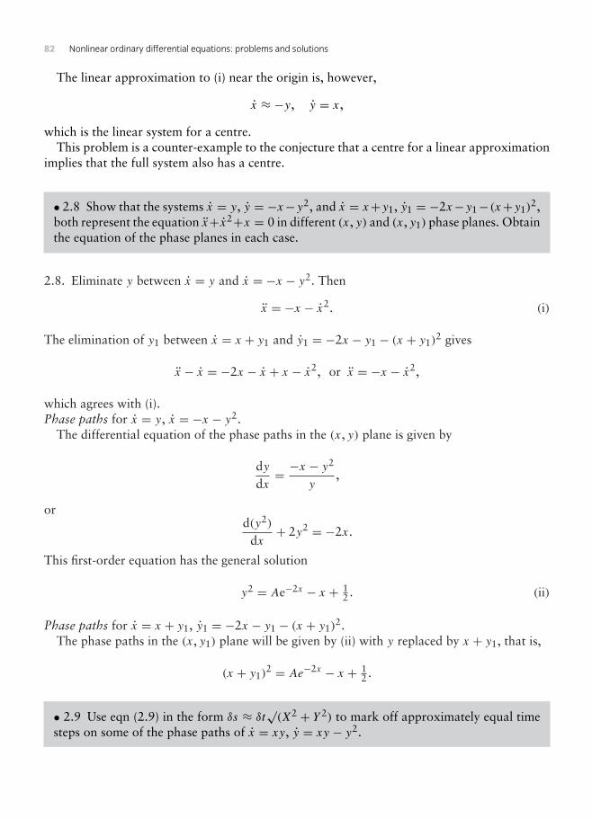
82 Nonlinear ordinary differential equations: problems and solutions
The linear approximation to (i) near the origin is, however,
x ≈ −y, y = x,
which is the linear system for a centre.This problem is a counter-example to the conjecture that a centre for a linear approximation
implies that the full system also has a centre.
• 2.8 Show that the systems x = y, y = −x−y2, and x = x+y1, y1 = −2x−y1−(x+y1)2,
both represent the equation x+x2+x = 0 in different (x, y) and (x, y1) phase planes. Obtainthe equation of the phase planes in each case.
2.8. Eliminate y between x = y and x = −x − y2. Then
x = −x − x2. (i)
The elimination of y1 between x = x + y1 and y1 = −2x − y1 − (x + y1)2 gives
x − x = −2x − x + x − x2, or x = −x − x2,
which agrees with (i).Phase paths for x = y, x = −x − y2.
The differential equation of the phase paths in the (x, y) plane is given by
dydx= −x − y2
y,
ord(y2)
dx+ 2y2 = −2x.
This first-order equation has the general solution
y2 = Ae−2x − x + 12 . (ii)
Phase paths for x = x + y1, y1 = −2x − y1 − (x + y1)2.
The phase paths in the (x, y1) plane will be given by (ii) with y replaced by x + y1, that is,
(x + y1)2 = Ae−2x − x + 1
2 .
• 2.9 Use eqn (2.9) in the form δs ≈ δt√(X2 + Y 2) to mark off approximately equal timesteps on some of the phase paths of x = xy, y = xy − y2.

2 : Plane autonomous systems and linearization 83
1 1x
1
1
(a) (b)y
1x
1
y
a
b
Figure 2.21 Problem 2.9: x = xy, y = xy−y2. (a) Shows the general features of the phase diagram, whilst (b) showsa smaller section of the phase diagram in the first quadrant marked at equal time intervals.
2.9. All points on the x axis are equilibrium points of the system x = xy, y = xy − y2. Thedifferential equation for the phase paths is given by
dydx= xy − y2
xy= x − y
x,
which is the same equation as that for the linear system x = x, y = x − y. The parameters forthis linear system, which has an equilibrium point at the origin, are p = 0, q = −1 < 0 whichsignifies a saddle point. Therefore the phase paths of this saddle point are the same as those ofthe nonlinear equation but the sense of the paths are different as shown in Figure 2.21(a), sincethe x axis is a line of equilibrium points.
In Figure 2.21(b), the formula for an element of arc of length δs ≈ δt√(X2 + Y 2), where
X = xy and Y = xy−y2, has been used. Two sets of equal time steps starting at a : (0.25, 0.125)and b : (0.1, 1) are shown by the succession of dots in the direction of the paths. For these timesteps δt = 1 was chosen.
• 2.10 Obtain approximations to the phase paths described by eqn (2.12) in the neighbour-hood of the equilibrium point x = b/d, y = a/c for the predator–prey problem x = ax−cxy,y = −by+dxy, (a, b, c, d) > 0 (see NODE, Example 2.3). (Write x = b/d+ ξ , y = a/c+η,and expand the logarithms to second-order terms in ξ and η.)
2.10. The phase paths for the predator–prey problem
x = ax − cxy, y = −by + dxy,
are given by (see eqn (2.12))
a ln y + b ln x − cy − xd = C.

84 Nonlinear ordinary differential equations: problems and solutions
The equations have an equilibrium point at (b/d, a/c). Close to this equilibrium point let
x = b
d+ ξ , y = a
c+ η.
Then
a ln y + b ln x − cy − xd
= a ln(ac+ η
)+ b ln
(b
d+ ξ
)− c
(ac+ η
)− d
(b
d+ ξ
)
= ln(ac
)+ a ln
(1+ cη
a
)+ b ln
(b
d
)+ b ln
(1+ dξ
b
)− a − cη − b − dξ
≈ −(a + b)+ a(cη
a− c2η2
2a2
)+ b
(dξ
b− d2ξ2
2b2
)− cη − dξ
= −(a + b)− d2ξ2
2b− c2η2
2a,
using standard Taylor expansions for the logarithms. Therefore close to the equilibrium pointthe phase paths are ellipses with equation
d2ξ2
b+ c2η2
a= constant.
• 2.11 For the system x = ax + by, y = cx + dy, where ad − bc = 0, show that all pointson the line cx + dy = 0 are equilibrium points. Sketch the phase diagram for the systemx = x − 2y, y = 2x − 4y.
2.11. For the linear system x = ax+by, y = cx+dy, the parameters are p = a+d, q = ad−bcand = p2 − 4q = (a + d)2 > 0. Equilibrium points are given by
ax + by = 0, cx + dy = 0.
Since ad − bc = 0, there are solutions other than x = 0, y = 0 which means that x and y cansatisfy both equations. Hence all points on cx + dy = 0 (or, equivalently, ax + by = 0) areequilibrium points.
For the particular problem, x = x − 2y, y = 2x − 4y, ad − bc = −4 + 4 = 0, so that allpoints on the line x − 2y = 0 are equilibrium points. The phase paths are given by
dydx= 2x − 4y
x − 2y= 2,
which has the general solution y = 2x+C. The phase paths are parallel straight lines with thesense of the paths as shown in Figure 2.22.

2 : Plane autonomous systems and linearization 85
–1
–1
1x
1y
Figure 2.22 Problem 2.11: x = x − 2y, y = 2x − 4y: equilibrium points lie on the line x = 2y.
• 2.12 The interaction between two species is governed by the deterministic model H =(a1 − b1H − c1)H , P = (−a2 + c2H)P , where H is the population of the host (prey),and P is that of the parasite (or predator), all constants being positive. (Compare NODE,Example 2.3: the term −b1H
2 represents interference with the host population when it getstoo large.) Assuming that a1c2 − b1a2 > 0, find the equilibrium states for the populations,and find how they vary with time from various initial populations.
2.12. The host(H)–parasite(P ) problem is governed by the model
H = (a1 − b1H − c1P)H , P = (−a2 + c2H)P .
The system is in equilibrium at the points (order (H ,P))
(0, 0),(a1
b1, 0
),
(a2
c2,a1c2 − b1a2
c1c2
)=
(a2
c2,D
c1c2
),
say, where D = a1c2 − b1a2.
I. (0, 0). Near the originH ≈ a1H , P ≈ −a2P .
This is a saddle point with separatrices P = 0 and H = 0.
II. (a1/b1, 0). Let H = (a1/b1)+ ξ . Then near the equilibrium point,
ξ ≈ −a1ξ − c1a1
b1P , P ≈ a1c2 − a2b1
b1.
The parameters for the linear approximation are
p = −a1 + D
b1, q = −a1D
b1< 0.

86 Nonlinear ordinary differential equations: problems and solutions
Hence this equilibrium point is also a saddle point.
III. (a2/c2,D/(c1c2)). LetH = a2
c2+ ξ , P = D
c1c2+ η.
Then
ξ =[a1 − b1
(a2
c2+ ξ
)− c1
(D
c1c2+ η
)](a2
c2+ ξ
)
≈ −a2b1
c2ξ − a2c1
c2η,
andη ≈ D
c1ξ .
The parameters associated with this linear approximation are
p = −a2b1
c2> 0, q = a2D
c2> 0, = a2
2b21
c22
− 4a2D
c2.
Therefore the equilibrium point is
a stable spiral if >a2b
21
4c2, or a stable node if <
a2b21
4c2.
Figure 2.23 shows the phase diagram for the system
H = (2−H − P)H , P = (−1+H)P ,
for which p = −1, q = 1 > 0 and = −3 < 0 at (1, 1). Therefore the equilibrium point islocally a stable spiral.
1 2H
1
2
P
Figure 2.23 Problem 2.12: H = (2−H − P)H , P = (−1+ xH)P .

2 : Plane autonomous systems and linearization 87
• 2.13 With the same terminology as in Problem 2.12, analyze the system H = (a1 − b1H − c1P)H , P = (a2 − b2P + c2H)P , all the constants being positive. (In this modelthe parasite can survive on alternative food supplies, although the prevalence of the hostencourages growth in population.) Find the equilibrium states. Confirm that the parasitepopulation can persist even if the host dies out.
2.13. In this model of host–parasite (H ,P) populations
H = (a1 − b1H − c1P)H , P = (a2 − b2P + c2H)P .
There are equilibrium points at (0, 0), (a1/b1, 0), (0, a2/b2) and
(a1b2 − c1a2
b1b2 + c1c2 ,a2b1 + a1c2
b1b2 + c1c2)
,
provided a1b2 ≥ c1a2.The parasite population can persist if the parameters satisfy a1b2 = c1a2, which is consistent
with the existence of an alternative food supply.
• 2.14 Consider the host–parasite population model H = (a1 − c1P)H , P = (a2 −c2(P /H))P , where the constants are positive. Analyse the system in the H ,P plane.
2.14. In this model of host–parasite (H ,P) populations
H = (a1 − c1P)H , P =(a2 − c2P
H
)P ,
where H > 0. The populations have one equilibrium state, at
(H ,P) =(a1c2
a2c1,a1
c1
).
Note that the P axis is a singular line since P is unbounded there.Let
H = a1c2
a2c1+ ξ , P = a1
c1+ η.
Then
ξ = (a1 − a1 − c1η)(a1c2
a2c1+ ξ
)≈ −a1c2η
a2,

88 Nonlinear ordinary differential equations: problems and solutions
and
η =[a2 − c2
(a1
c1+ η
)(a1c2
a2c1+ ξ
)−1](
a1
c1+ η
)≈ a2
2
c2ξ − a2η.
The parameters associated with this linear approximation are
p = −a2 < 0, q = a1a2 > 0, = a22 − 4a1a2.
Therefore by the table in Section 2.5, the equilibrium point is a stable node if a2 > 4a1 and astable spiral if a2 < 4a1.
• 2.15 In the population model F = −αF +βµ(M)F , M = −αM+γµ(M)F , where α > 0,β > 0, γ > 0, F and M are the female and male populations. In both cases the death ratesare α. The birth rate is governed by the coefficient µ(M) = 1 − e−kM , k > 0, so that forlarge M the birth rate for females is βF and that for males is γF , the rates being unequalin general. Show that if β > α then there are two equilibrium points, at (0, 0) and at(
− β
γ kln
[β − αβ
],−1k
ln[β − αβ
]).
Show that the origin is stable and that the other equilibrium point is a saddle point, accordingto their linear approximations. Verify that M = γF/β is a particular solution. Sketch thephase diagram and discuss the stability of the populations.
2.15. A male–female population is modelled by the birth and death equations
F = −αF + βµ(M)F , M = −αM + γµ(M)F , (i)
where µ(M) = 1− e−kM . Equilibrium occurs where
−F [α + β(1− e−kM)] = 0, −αM + γ (1− e−kM)F = 0.
The equations have two equilibrium points; at
(0, 0) and(− β
γ kln
[β − αβ
],−1k
ln[β − αβ
])
in the (F ,M) plane.I. (0, 0). Near the origin
F ≈ −αF , M ≈ −αM.
The phase paths are given by
dMdF
= M
F,

2 : Plane autonomous systems and linearization 89
so that M = CF , where C is an arbitrary constant. The paths are are straight lines into theorigin, which implies that the origin is stable.
II. For the other equilibrium point, let
(F0,M0) =(− β
γ kln
[β − αβ
],−1k
ln[β − αβ
]).
Let F = F0 + ξ and M = M0 + η Then, from (i),
ξ = −α(F0 + ξ)+ β(1− e−k(M0+η))(F0 + ξ)≈ −αF0 − αξ + β[1− e−kM0(1− kη)](F0 + ξ)= βkF0e−kM0η
= −β(β − α)γ
ln[β − αβ
]η.
η = −α(M0 + η)+ γ (1− e−k(M0+η))(F0 + ξ)≈ −αM0 − αη + γ [1− e−kM0(1− kη)](F0 + ξ)= αγ
βξ + (−α + γ ke−kM0F0)η
= αγ
βξ −
(α + (β − α) ln
[β − αβ
])η.
The parameters associated with this linear approximation are
p = −(α + (β − α) ln
[β − αβ
]), q = α(β − α) ln
[β − αβ
]< 0.
Hence (F0,M0) is a saddle point.
1 2 3F
1
2M
(F0, M0)
Figure 2.24 Problem 2.15: Population model with α = 0.5, β = 1, γ = 0.5 and k = 1.

90 Nonlinear ordinary differential equations: problems and solutions
It can be verified by direct substitution in the differential equations that M = γF/β satisfiesboth equations, and therefore defines two phase paths which are separatrices through the saddlepoint. The phase diagram with parameters α = 0.5, β = 1, γ = 0.5 and k = 1 is shown inFigure 2.24.
• 2.16 A rumour spreads through a closed population of constant size N + 1. At time t thetotal population can be classified into three categories:x persons who are ignorant of the rumour;y persons who are actively spreading the rumour;z persons who have heard the rumour but have stopped spreading it: if two persons whoare spreading the rumour meet then they stop spreading it.The contact rate between any two categories is a constant, µ.Show that the equations
x = −µxy, y = µ[xy − y(y − 1)− yz]give a deterministic model of the problem. Find the equations of the phase paths and sketchthe phase diagram.Show that, when initially y = 1 and x = N , the number of people who ultimately neverhear the rumour is x1, where
2N + 1− 2x1 +N ln(x1/N) = 0.
2.16. In incremental form the equations are the limits as δt → 0 of
δx = −µxyδt , δy = µ[xy − y(y − 1)− yz]δt .
Contact frequencies between any two groups are assumed to be proportional to the product ofthe population sizes. Thus, the decrease in the number of those who do not know the rumour−δx must be proportional to xyδt , and the number δy of those who are actively spreading therumour must increase at a rate proportional to contacts between x and y, and decrease at a rateproportional to meetings between spreaders, y(y − 1), and between y and those who alreadyknow, z. Hence
δy = µ[xy − y(y − 1)− yz]δt ,and the differential equation follows in the limit δt → 0. Since the population has constant sizeN + 1, the third equation is x + y + z = N = 1.
Substitute for z in the differential equations in the question. Then x and y satisfy
x = −µxy, y = µ[xy − y(y − 1)− y(N + 1− x − y)] = µ(2xy −Ny). (i)
Therefore the differential equation for the phase paths is
dydx= y
x= N − 2x
x.

2 : Plane autonomous systems and linearization 91
100 200x
100
200
y
x+y = N+1
Figure 2.25 Problem 2.16: Epidemic model with N = 200.
This is a separable first-order equation with general solution
y =∫ (
N
x− 2
)dx = N ln x − 2x + C, (x > 0). (ii)
The second equation in (i) has the solution y = 0, which must correspondence to a line ofequilibrium points since x = 0 also. In the model this means that no one is spreading therumour, but there may be a (constant) number of individuals who do not know the rumour.Linearization is not really helpful since the points on the x axis will be non-standard equilibriumpoints. The phase paths can be plotted using the curves given by (ii): some phase paths are shownin Figure 2.25. Note that x + y ≤ N , so that the phase diagram is bounded by this line.
If the initial conditions are y = 1 and x = N , then, from (ii)
1 = N lnN − 2N + C, so that C = 2N + 1−N lnN .
Hence on this pathy = N ln x −N lnN − 2x + 2N + 1.
The number of individuals x1 who never hear the rumour occurs where y = 0. Therefore x1satisfies
N ln x1 −N lnN − 2x1 + 2N + 1 = 0.
• 2.17 The one-dimensional steady flow of a gas with viscosity and heat conduction satisfiesthe equations
µ0
ρc1
dvdx= √(2v)[2v −√(2v)+ θ],
k
gRρc1
dθdx= √(2v)
[θ
γ − 1− v +√(2v)− c
],
where v = u2/(2c1)2, c = c22/c
21 and θ = gRT /c2
1 = p/(ρc21). In this notation, x is measured
in the direction of flow, u is the velocity, T is the temperature, ρ is the density, p the pressure,
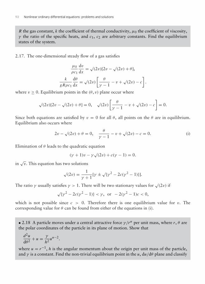
92 Nonlinear ordinary differential equations: problems and solutions
R the gas constant, k the coefficient of thermal conductivity, µ0 the coefficient of viscosity,γ the ratio of the specific heats, and c1, c2 are arbitrary constants. Find the equilibriumstates of the system.
2.17. The one-dimensional steady flow of a gas satisfies
µ0
ρc1
dvdx= √(2v)[2v −√(2v)+ θ ],
k
gRρc1
dθdx= √(2v)
[θ
γ − 1− v +√(2v)− c
].
where v ≥ 0. Equilibrium points in the (θ , v) plane occur where
√(2v)[2v −√(2v)+ θ] = 0,
√(2v)
[θ
γ − 1− v +√(2v)− c
]= 0.
Since both equations are satisfied by v = 0 for all θ , all points on the θ are in equilibrium.Equilibrium also occurs where
2v −√(2v)+ θ = 0,θ
γ − 1− v +√(2v)− c = 0. (i)
Elimination of θ leads to the quadratic equation
(γ + 1)v − γ√(2v)+ c(γ − 1) = 0.
in√v. This equation has two solutions
√(2v) = 1
γ + 1[γ ±√γ 2 − 2c(γ 2 − 1)].
The ratio γ usually satisfies γ > 1. There will be two stationary values for√(2v) if
√γ 2 − 2c(γ 2 − 1) < γ , or − 2(γ 2 − 1)c < 0,
which is not possible since c > 0. Therefore there is one equilibrium value for v. Thecorresponding value for θ can be found from either of the equations in (i).
• 2.18 A particle moves under a central attractive force γ /rα per unit mass, where r, θ arethe polar coordinates of the particle in its plane of motion. Show that
d2u
dθ2 + u =γ
h2uα−2.
where u = r−1, h is the angular momentum about the origin per unit mass of the particle,and γ is a constant. Find the non-trivial equilibrium point in the u, du/dθ plane and classify

2 : Plane autonomous systems and linearization 93
it according to its linear approximation. What can you say about the stability of the circularorbit under this central force?
2.18. In Figure 2.26, the position of the particle of mass m is (r, θ) in polar coordinates. Theradial and transverse equations of motion are, under the influence of the central forcemγ/rα are
−mγrα
= m(r − rθ2), (i)
mddt(r2θ ) = 0. (ii)
From (ii) it follows thatmr2θ = constant = mh, (iii)
say, where mh is the (constant) angular momentum of the particle. Now eliminate θ between(i) and (ii) so that
r − h2
r3 = −γ
rα. (iv)
Using the identity
r = θ ddθ
(θ
drdθ
),
and the change of variable u = 1/r, eqn (iv) can be expressed in the form
d2u
dθ2 + u =γ
h2uα−2.
Let ν = du/dθ . Then the differential equation of the phase paths in the (θ ,p) plane is
dνdθ= k
h2uα−2 −u.
r
m
mr
Figure 2.26 Problem 2.18.

94 Nonlinear ordinary differential equations: problems and solutions
There are equilibrium points; at u = 0 (physically of no interest) and at u = u0 = (h2/k)1/(α−3)
provided α = 3, in which case there is just one equilibrium point at u = 0.Let u = u0 + u′,where |u′| is small. Then
dνdθ= k
h2
(u0 + u′
)α−2 − u0 − u′
≈ k
h2uα−20
[1+ (α − 2)
(u′
u0
)]− u0 − u′
= (α − 3)u′
Hence the linear approximation of the equilibrium point indicates that it is a centre if α < 3,and a saddle point α > 3.
The equilibrium point u = u0, ν = 0 corresponds to a circular orbit of the particle, which isstable if α < 3 and unstable if α > 3. The gravitational inverse-square law gives a stable orbit.
• 2.19 The relativistic equation for the central orbit of a planet is
d2u
dθ2 + u = k + εu2,
where u = 1/r, and r, θ are the polar coordinates of the planet in the plane of its motion. Theterm εu2 is the ‘Einstein correction’, and k and ε are positive constants, with ε very small.Find the equilibrium point which corresponds to a perturbation of the Newtonian orbit.Show that the equilibrium point is a centre in the u, du/dθ plane according to the linearapproximation. Confirm this by using the potential energy method of NODE, Section 1.3.
2.19. The relativistic equation is
d2u
dθ2 + u = k + εu2 (i)
(see Problem 2.19). Aside from the correction term k, the polar equation can be derived as inProblem 2.18 assuming the inverse-square law. The equilibrium points are given by
εu2 − u+ k = 0,
that is,
u =u1u2
= 12ε[1±√(1− 4kε)).

2 : Plane autonomous systems and linearization 95
5 10u
–4
4
5 10u
5
V(u)
V
Figure 2.27 Problem 2.19: The phase diagram for the relativistic equation has been computed for k = 1 and ε = 0.1:the equilibrium points are at u = 1.127 and u = 8.873.
Let ν = du/dθ , and u = ui + u′i , (i = 1, 2), where |u′i | is small. Substituting into (i), we have
d2u′idθ2 = −ui − u′i + k + ε(ui + u′i )2
≈ −ui − u′i + k + u2i + 2uiu′i
= ±√(1− 4kε)u′i
Hence u1 is a saddle, and u2 is a centre, assuming that ε is sufficiently small to make 4kε < 1.In the notation of Section 1.3, the potential associated with eqn (i) is
V(u) = −∫(k + εu2 − u)du = −ku− 1
3εu3 + 1
2u2.
A graph of the potential V(u) and the corresponding phase diagram are shown in Figure 2.27.The equilibrium points correspond to circular orbits. In terms of r =1/u, the inner orbit isunstable whilst the outer orbit is stable.
• 2.20 A top is set spinning at an axial rate n about its pivotal point, which is fixed in space.The equations of its motion, in terms of the angles θ and µ are (see Figure 2.14 in NODE)
Aθ − A(+ µ)2 sin θ cos θ + Cn(+ µ) sin θ −Mgh sin θ = 0,
Aθ2 + A(+ µ)2 sin2 θ + 2Mgh cos θ = E;
where (A,A,C) are the principal moments of inertia about O, M is the mass of the top, his the distance between the mass centre and the pivot, and E is a constant. Show that anequilibrium state is given by θ = α, after elimination of between
A2 cosα − Cn+Mgh = 0, and A2 sin2 α + 2Mgh cosα = E.

96 Nonlinear ordinary differential equations: problems and solutions
Suppose that E = 2Mgh, so that θ = 0 is an equilibrium state. Show that, close to thisstate, θ satisfies
Aθ + [(C − A)2 −Mgh]θ = 0.
For what condition on is the motion stable?
2.20. The equations of the motion of the top in terms of the angles θ and µ are
Aθ − A(+ µ)2 sin θ cos θ + Cn(+ µ) sin θ −Mgh sin θ = 0, (i)
Aθ2 + A(+ µ)2 sin2 θ + 2Mgh cos θ = E. (ii)
µ can be eliminated between these equations to obtain a second-order differential equation inθ . The equilibrium states of the top are then given by putting θ = 0 and θ = 0 in this equationin θ , but this is equivalent to the elimination of between (i) and (ii) with both θ and µ zero,that is, between
(−A2 cos θ + Cn−Mgh) sin θ = 0, (iii)
and
A2 sin2 θ + 2Mgh cos θ = E. (iv)
If E = 2Mgh, then eqn (iv) becomes
A2 sin2 θ = 2Mgh(1− cos θ).
Hence θ = 0 is a solution of this equation and (iii), and must be an equilibrium point in whichthe top spins about its axis; which is vertical. Also in this state = n and µ = 0. For small |θ |,eqn (i) becomes
θ + [(C − A)2 −Mgh]θ ≈ 0.
The vertical spin is stable if (C − A)2 > Mgh.
• 2.21 Three gravitating particles with gravitational masses µ1, µ2, µ3, move in a planeso that they always remain at the vertices of an equilateral triangle P1P2P3 with varyingside-length a(t) as shown in Figure 2.15 (in NODE). The triangle rotates in the plane with

2 : Plane autonomous systems and linearization 97
spin (t) about the combined mass-centre G. If the position vectors of the particles are r1,r2, r3, relative to G, show that the equations of motion are
ri = −µ1 + µ2 + µ3
a3 ri , (i = 1, 2, 3).
If |ri | = ri , deduce the polar equations
ri − ri2 = −µ1 + µ2 + µ3
a3 ri , r2i = constant, (i = 1, 2, 3).
Explain why a satisfies
a − a2 = −µ1 + µ2 + µ3
a2 , a2 = constant = K,
say, and that solutions of these equations completely determine the position vectors. Expressthe equation in non-dimensionless form by the substitutions a = K2/(µ1 + µ2 + µ3),t = K3τ/(µ1 + µ2 + µ3)
2, sketch the phase diagram for the equation in u obtained byeliminating , and discuss possible motions of this Lagrange configuration.
2.21. The configuration is shown in Figure 2.28. Since G is the mass-centre,
µ1r1 + µ2r2 + µ3r3 = 0. (i)
The equation of motion fo P1 is
µ1r1 = −µ1µ2(r2 − r1)a3 − µ1µ3(r3 − r1)
a3 ,
or, using (i),
r1 = − (µ1 + µ2 + µ3)
a3 r1,
with similar equations for r2 and r3.
G
P1
P3
P2
r1
r2r3 1 2u
–0.5
0.5
v
Ω
Figure 2.28 Problem 2.21: Lagrange equilateral configuration for a three-body problem with P1P2 = P2P3 =P3P1 = a(t): phase diagram in (u, v) plane.

98 Nonlinear ordinary differential equations: problems and solutions
In fixed axes let the polar equations of P1 be r1 = |r1| and θ1. Since the triangle rotates withspin , it follows that θ1 = . Similarly for P2 and P3, the other polar angles also satisfyθ2 = θ3 = . The radial and transverse polar equations are therefore
ri − ri θ2i = ri − ri2 = −µ1 + µ2 + µ3
a3 ri , (ii)
andddt(r2i θi ) = 0, which implies r2
i θi = r2i = constant. (iii)
for i = 1, 2, 3.Throughout the motion, the equilateral triangle varies in size as it rotates, but the ratio r1/a
remains constant with time, and similarly for r2/a and r3/a. From (ii) and (iii), it followsthat
a − a2 = −µ1 + µ2 + µ3
a2 , (iv)
anda2 = constant = K, (say). (v)
Elimination of between (iv) and (v) leads to
a − K2
a3 = −µ1 + µ2 + µ3
a2 , (a > 0).
The equation can be expressed in the dimensionless form
d2u
dτ2 = u′′ =1− uu3 , (u > 0),
using the substitutions a = K2u/(µ1 + µ2 + µ3), t = K3τ/(µ1 + µ2 + µ3)2.
If v = u′, then the equation for the phase paths is
vdvdu= 1− u
u3 ,
which has the general solution
v2 = − 1u2 +
2u+ C.
In the (u, v) phase plane, the system has a single equilibrium point at u = 1, which is acentre (see Figure 2.28). This implies that the lengths of the sides of the equilateral triangleoscillate with time. The fixed point corresponds to a Lagrange motion in which the threemasses remain at the vertices of a fixed equilateral triangle as they rotate in circular orbitsaboutG. (For information, in general, the orbits are similar ellipses although this is not provedhere.)

2 : Plane autonomous systems and linearization 99
• 2.22 A disc of radius a is freely pivoted at its centre A so that it can turn in a verticalplane . A spring, natural length 2a and stiffness λ connects a point B on the circumferenceof the disc to a fixed pont O, distance 2a above A. Show that θ satisfies
I θ = −T a sinφ, T = λa[(5− 4 cos θ)1/2 − 2],where T is the tension in the spring, I is the moment of inertia of the disc aboutA, OAB = θ ,and ABO = φ. Find the equilibrium states of the disc, and their stability.
2.22. The configuration of the system is shown in Figure 2.29. Taking moments about A,
−T a sin(π − φ) = I θ , or − T a sinφ = I θ , (i)
where, from triangle ABO, using the sine and cosine rules,
OB
sin θ= 2a
sinφ, OB2 = 4a2 + a2 − 4a2 cos θ .
Elimination of OB between these equations leads to
sinφ = 2a sin θOB
= 2 sin θ√(5− 4 cos θ)
. (ii)
By Hooke’s law the tension,
T = λ(OB − 2a) = λa[√(5− 4 cos θ)− 2]. (iii)
where λ is a constant. Elimination of T and φ between eqns (i), (ii) and (iii) leads to thedifferential equation for θ :
I θ + 2λa2[1− 25− 4 cos θ)−(1/2)] sin θ = 0.
O
A
B
au
f
Figure 2.29 Problem 2.22.
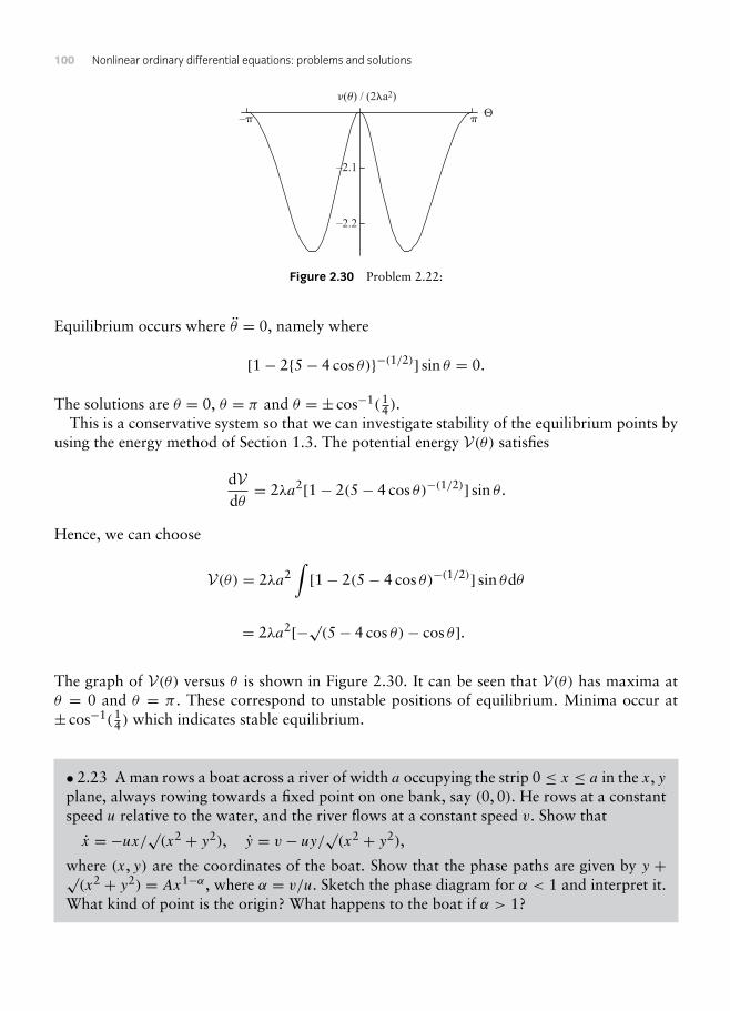
100 Nonlinear ordinary differential equations: problems and solutions
–2.2
–2.1
–
(u) / (2a2)
Θ
Figure 2.30 Problem 2.22:
Equilibrium occurs where θ = 0, namely where
[1− 25− 4 cos θ)−(1/2)] sin θ = 0.
The solutions are θ = 0, θ = π and θ = ± cos−1(14 ).
This is a conservative system so that we can investigate stability of the equilibrium points byusing the energy method of Section 1.3. The potential energy V(θ) satisfies
dVdθ
= 2λa2[1− 2(5− 4 cos θ)−(1/2)] sin θ .
Hence, we can choose
V(θ) = 2λa2∫[1− 2(5− 4 cos θ)−(1/2)] sin θdθ
= 2λa2[−√(5− 4 cos θ)− cos θ ].
The graph of V(θ) versus θ is shown in Figure 2.30. It can be seen that V(θ) has maxima atθ = 0 and θ = π . These correspond to unstable positions of equilibrium. Minima occur at± cos−1(1
4 ) which indicates stable equilibrium.
• 2.23 A man rows a boat across a river of width a occupying the strip 0 ≤ x ≤ a in the x, yplane, always rowing towards a fixed point on one bank, say (0, 0). He rows at a constantspeed u relative to the water, and the river flows at a constant speed v. Show that
x = −ux/√(x2 + y2), y = v − uy/√(x2 + y2),
where (x, y) are the coordinates of the boat. Show that the phase paths are given by y +√(x2 + y2) = Ax1−α, where α = v/u. Sketch the phase diagram for α < 1 and interpret it.
What kind of point is the origin? What happens to the boat if α > 1?

2 : Plane autonomous systems and linearization 101
x
y
O
u
u
v
(x,y)
a
Figure 2.31 Problem 2.23.
2.23. A plan view of the river and the boat is shown in Figure 2.31. If (x, y) are the coordinatesof the boat and the θ is the angle between the x axis and the radius to the boat, then the velocitycomponents (x, y) of the boat are given by
x = −u cos θ = − ux√(x2 + y2)
,
y = v − u sin θ = v − uy√(x2 + y2)
,
since the boat always points towards the origin. The phase paths are given by
dydx= y
x= uy − v√(x2 + y2)
ux.
This is a first-order homogeneous equation for which we use the substitution y = wx. Thereforethe equation becomes, in terms of w and x,
xdwdx+ w = uw − v√(1+ w2)
u,
or
xdwdx
= −vu
√(1+ w2).
This is a separable equation with solution
∫dw√
(1+ w2)= −v
u
∫dxx= −v
uln x + C, (x > 0),

102 Nonlinear ordinary differential equations: problems and solutions
x
y
O
a
Figure 2.32 Problem 2.23: Phase diagram with α = 12 and a = 1.
where C is an arbitrary constant. For the left-hand side use the substitution w = tan θ so that
∫dw√
(1+ w2)=
∫sec θdθ = ln(sec θ + tan θ)
= ln[√(1+ w2)+ w] = [√(x2 + y2)+ y]/x.
Therefore the solution can be expressed in the implicit form
y = −√(x2 + y2)+ Ax1−α. (i)
whereA is a positive constant and α = v/u. The origin is a singular point (i.e. not an equilibriumpoint) where solutions of the differential equations cross. A phase diagram for α = 0.5 anda = 1 is shown in Figure 2.32.
If α > 1, then the river flow speed is greater than the speed of the boat. From (i) it can beseen that the paths no longer pass through the origin. The rower cannot reach the origin fromany point on the opposite bank.
• 2.24 In a simple model of a national economy, I = I − αC, C = β(I − C − G), whereI is the national income, C is the rate of consumer spending and G the rate of governmentexpenditure; the constants α and β satisfy 1 < α < ∞, 1 ≤ β < ∞. Show that if therate of government expenditure G0 is constant there is an equilibrium state. Classify theequilibrium state and show that the economy oscillates when β = 1.
Consider the situation when the government expenditure is related to the national incomeby the ruleG = G0+kI , where k > 0. Show that there is no equilibrium state if k ≤ (α−1)/α.How does the economy then behave?

2 : Plane autonomous systems and linearization 103
Discuss an economy in which G = G0 + kI2, and show that there are two equilibriumstates if G0 < (α − 1)2/(4kα2).
2.24. The economy model is governed by the equations
I = I − αC, C = β(I − C −G). (i)
(i) G = G0. Equilibrium occurs where
I − αC = 0, and I − C −G0 = 0,
which has the solution
C = G0
α − 1, I = αG0
α − 1.
The equations are linear so that we can read off the usual parameters from (i):
p = 1− β < 0, q = −β + αβ > 0,
= (1− β)2 − 4β(α − 1) = (1+ β)2 − 4βα.
From the table in Section 2.5, the equilibrium point is a stablenode if β > 1 and (1+β)2 > 4βα,and a stable spiral if β > 1 and (1+β)2 < 4βα. If β = 1, then the equilibrium point is a centre.In the latter case the economy will oscillate with amplitude which is dependent on the initialconditions.
(ii) G = G0 + kI . The model now becomes
I = I − αC, C = β[(1− k)I − C −G0]. (ii)
Equilibrium occurs where
C = G0
α − 1− kα , I = αG0
α − 1− kα .
If k < (α − 1)/α the equilibrium point is in the first quadrant: otherwise the model has noequilibrium there (since C and I must both be positive). At the equilibrium point the parametervalues are
p = 1− β < 0, q = β(α − 1− αk), = (1− β)2 − 4β(α − 1− αk).
The point is a saddle point if k > (α − 1)/α (in the third quadrant). If k < (α − 1)/α, then theequilibrium point, in the first quadrant, is a stable node if (1− β)2 > 4β(α− 1− k) or a stablespiral if (1− β)2 < 4β(α − 1− k). Two phase diagrams for the case k > (α − 1)/α are shownin Figure 2.33.

104 Nonlinear ordinary differential equations: problems and solutions
I
C(i)
4 8I
4
8
C(ii)
Figure 2.33 Problem 2.24: The phase diagrams are shown for the following parameters: (i) α = 2, β = 1, k = 2,G0 = 1; (ii) α = 2, β = 1, k = 3
4 , G0 = 1. The dashed lines show the isoclines of zero and infinite slopes.
(iii) G = G0 + kI2. The equations become
I = I − αC, C = β(I − C −G0 − kI2).
Equilibrium states are given by
I − αC = 0 β(I − C −G0 − kI2) = 0.
Eliminating I , C satisfies
C = 12kα2 (α − 1)±√[(α − 1)2 − 4G0kα
2]
and I can be found from I = αC. There are two real positive solutions ifG0 < (α−1)2/(4kα2).
• 2.25 Let f (x) and g(y) have local minima at x = a and y = b respectively. Show thatf (x) + g(y) has a minimum at (a, b). Deduce that there exists a neighbourhood (a, b) inwhich all solutions of the family of equations f (x)+g(y) = constant represent closed curvessurrounding (a, b).
Show that (0, 0) is a centre for the system x = y5, y = −x3, and that all paths are closedcurves.
2.25. Define the open intervals I1 : ε > |x − a| > 0 and I2 : ε > |y − b| > 0. Since f (x) has aminimum at x = a, and g(y) has a minimum at y = b, there exists an ε such that f (x) > f (a)for all x ∈ I1, and g(y) > g(b) for all y ∈ I2.
For the function of two variables f (x)+ g(y),f (x)+ g(y) > f (a)+ g(b) for all (x, y) ∈ I1 × I2.
Therefore (a, b) is a local minimum of f (x)+g(y), and for some neighbourhood of (a, b), thereexists a constant c1 > f (a, b) such that the curves f (x) + g(b) = c are closed curves about(a, b) for all C such that f (a, b) < c < c1.

2 : Plane autonomous systems and linearization 105
For the system
x = y5, y = −x3,
which has a single equilibrium point, at (0, 0), the phase paths are given by
dydx= −x
3
y5 .
The solutions are given by16y
6 + 14x
4 = constant.
In the notation above, let f (x) = 14x
4, which has a minimum at x = 0, and let g(y) = 16y
6,which has a minimum at y = 0. By the result above 1
6y6 + 1
4x4 has minimum at (0, 0). Hence,
the origin is surrounded by a nest of closed paths, and is therefore a centre.
• 2.26 For the predator–prey problem in NODE, Section 2.2, show, by using Problem 2.25,that all solutions in x > 0, y > 0 are periodic.
2.26. The predator–prey equations are, from Section 2.2,
x = ax − cxy, y = −by + dxy,
and the equation of the phase paths is
b ln x − dx + a ln y − cy = C,
a constant. Equilibrium occurs at (b/d, a/c). In the notation of Problem 2.25, let f (x) =b ln x − dx and g(y) = a ln y − cy. Since
f ′(x) = b
x− d, f ′′(x) = − b
x2 , g′(y) = a
y− c, g′′(y) = − a
y2 ,
it can be verified that f (x) has a minimum at x = b/d, and that g(y) has a minimum aty = a/c. The level curves of the surface f (x)+g(y) cover the whole of the first quadrant abouta minimum at (b/d, a/c), which is a centre. Hence all solutions are periodic about the centre.
• 2.27 Show that the phase paths of the Hamiltonian system x = −∂H/∂y, y = ∂H/∂x
are given by H(x, y) = constant. Equilibrium points occur at the stationary points ofH(x, y). If (x0, y0) is an equilibrium point, show that (x0, y0) is stable according to thelinear approximation if H(x, y) has a maximum or a minimum at the point. (Assume thatall the second derivatives of H are non-zero at x0, y0.)

106 Nonlinear ordinary differential equations: problems and solutions
2.27. A first-order system is said to be Hamiltonian if there exists a differentiable functionH(x, y) such that
x = −∂H∂y
, y = ∂H
∂x. (i)
The phase paths of the system are given by
dydx= −∂H/∂x
∂H/∂y,
which, using the chain rule, can be expressed in the form
∂H
∂x+ ∂H
∂y
dydx= dH(x, y)
dx= 0,
treating y as a function x. Therefore the general solution is H(x, y) = constant. Equilibriumpoints occur at the stationary points of H(x, y).
Let (x0, y0) be a stationary point of H(x, y). Consider the perturbation x = x0 + x′ andy = y0 + y′. Then eqns (i) become
x = −Hy(x0 + x′, y0 + y′)≈ −[Hy(x0, y0)+Hyx(x0, y0)x
′ +Hyy(x0, y0)y′]
= −Hyx(x0, y0)x′ −Hyy(x0, y0)y
′ = −Bx′ − Cy′,
say, and
y = Hx(x0 + x′, y0 + y′)≈ Hx(x0, y0)+Hxx(x0, y0)x
′ +Hxy(x0, y0)y′
= Hxx(x0, y0)x′ +Hxy(x0, y0)y
′ = Ax′ + By′
say, using the first two terms of the Taylor series in both cases. The second derivative test forfunctions of two variables says that (x0, y0) is a maximum or minimum if the second derivativessatisfy AC−B2 > 0. For the linear approximation above, the parameters are p = −B+B = 0and q = −B2 + AC. For stability we require q > 0 which is the same condition as for astationary maximum or minimum of H(x, y).
• 2.28 The equilibrium points of the nonlinear parameter-dependent system x = y, y =f (x, y, λ) lie on the curve f (x, 0, λ) = 0 in the x, λ plane. Show that an equilibrium point(x1, λ1) is stable and that all neighbouring solutions tend to this point (according to thelinear approximation) if fx(x1, 0, λ1) < 0 and fy(x1, 0, λ1) < 0.Investigate the stability if x = y, y = −y + x2 − λx.

2 : Plane autonomous systems and linearization 107
2.28. Consider the system x = y, y = f (x, y, λ). Equilibrium points occur where y = 0 andf (x, 0, λ). Let x = x1 + x′ and y = y′. The linear approximation is
x′ = y′, y′ = f (x1 + x′, y′, λ) ≈ fx(x1, 0, λ1)x′ + fy(x1, 0, λ)y′.
The parameters of the linear approximation are
p = fy(x1, 0, λ1), q = −fx(x1, 0, λ1).
The equilibrium point is stable if p < 0 and q > 0, which is equivalent to
fy(x1, 0, λ1) < 0, fx(x1, 0, λ1) < 0.
In the example
x = y, y = −y + x2 − λx,
f (x, y, λ) = −y+x2−λx. The equilibrium points are at (0, 0) and (λ, 0). The first derivatives are
fx(x, 0, λ) = 2x − λ, fy(x, 0, λ) = −1.
At (0, 0),
fx(0, 0, λ) = −λ < 0
if λ > 0, and
fy(0, 0, λ) = −1 < 0,
for all λ. Hence (0, 0) is stable if λ > 0.At (λ, 0),
fx
(12λ, 0, λ
)= λ < 0,
if λ < 0, and
fy
(12λ, 0, λ
)= −1.
Therefore the point (λ, 0) is stable if λ < 0.
• 2.29 Find the equations for the phase paths for the general epidemic described(Section 2.2) by the system
x = −βxy, y = βxy − γ y, z = γ y.
Sketch the phase diagram in the (x, y) plane. Confirm that the number of infectives reachesits maximum when x = γ /β.

108 Nonlinear ordinary differential equations: problems and solutions
1 2 3 4x
1
2y
Figure 2.34 Problem 2.29: The phase diagram is drawn for γ /β = 1.
2.29. The general epidemic equations are
x − βxy, y = βxy − γ y, z = γ y
(see Example 2.4). From the first two equations equilibrium occurs at y = 0 for all x ≥ 0. Thephase paths in the x, y plane are given by
dydx= y
x= −βx − γ
βx.
This is a separable equation with general solution
y = −∫βx − γβx
dx = −x + γ
βln x + C,
noting that both x and y must be positive. A phase diagram is shown in Figure 2.34. From theequation y = βxy−γ y, y = 0 where x = γ /β. The maxima lie on the line x = 1 in Figure 2.34where dy/dx = 0.
• 2.30 Two species x and y are competing for a common food supply. Their growthequations are
x = x(1− x − y), y = y(3− x − 32y), (x, y > 0).
Classify the equilibrium points using linear approximations. Draw a sketch indicating theslopes of the phase paths in x ≥ 0, y ≥ 0. If x = x0 > 0, y = y0 > 0 initially, what do youexpect the long-term outcome of the species to be? Confirm your conclusions numericallyby computing phase paths.
2.30. The system
x = x(1− x − y), y = y(3− x − 3
2y)

2 : Plane autonomous systems and linearization 109
is in equilibrium at (0, 0), (0, 2) and (1, 0), the solutions of
x(1− x − y) = 0, and y(3− x − 3
2y)= 0.
• (0, 0). The linear approximation is
x ≈ x, y ≈ 3y,
which is an unstable star-shaped equilibrium point;
• (0, 2). Let x = ξ , y = 2+ η. Then
ξ = ξ [1− ξ − (2+ η)] ≈ −ξ , η = (2+ η)[3− ξ − 3
2(2+ η)
]≈ −2ξ − 3η,
which implies a stable node.
• (1, 0). Let x = 1+ ξ , y = η. The
ξ = (1+ ξ)[1− (1+ ξ)− η] ≈ −ξ − η, η = η[3− (1+ ξ)− 3
2η
]≈ 2η,
which implies a saddle.
The isoclines on which dy/dx=0 are the straight lines y=0 and 3−x− 32y=0, and the isoclines
on which dy/dx=∞ are x = 0 and 1 − x − y=0. These are shown in Figure 2.35 togetherwith the signs of the slopes of the paths between these lines. The computed phase diagram isalso shown in this figure. For any initial point x= x0 > 0, y= y0 > 0, all phase paths approach(0, 2) asymptotically, which means that species x ultimately dies out.
1 2 3x
1
2
y
A B
C
y = 1 – x
3y = 6 – 2x
Figure 2.35 Problem 2.30: The phase diagram for x = x(1− x − y), y = y(3− x − 32y). In the phase diagram, A is
the region in which x > 0, y > 0, B is the region in which x < 0, y > 0 and C is the region in which x < 0, y < 0.

110 Nonlinear ordinary differential equations: problems and solutions
• 2.31 Sketch the phase diagram for the competing species x and y for which
x = (1− x2 − y2)x, y = (54 − x − y)y.
2.31. The competing species equations are
x = (1− x2 − y2)x, y = (1.25− x − y)y.
In the the quadrant x ≥ 0, y ≥ 0, the equilibrium points are given by
(0, 0), (0, 1.250), (1, 0), (0.294, 0.956), (0.956, 0.294).A computed phase diagram is shown in Figure 2.36. The dashed line and arc are respectivelythe isoclines of zero and infinite slopes. From the figure we can see that (0, 0) is a unsta-ble star-shaped point. The points (1, 0) and (0.294, 0.956) are saddle points, and (0, 1) and(0.956, 0.294) are stable nodes. These interpretations from the phase diagram can be confirmedby finding the linear approximations at each equilibrium point.
1x
1
y
A B
Figure 2.36 Problem 2.31: The phase diagram for x = x(1− x2 − y2), y = y(1.25− x − y).
• 2.32 A space satellite is in free flight on the line joining, and between, a planet (mass m1)and its moon (mass m2), which are at a fixed distance a apart. Show that
−γm1
x2 + γm2
(a − x)2 = x,
where x is the distance of the satellite from the planet and γ the gravitational constant.Show that the equilibrium point is unstable according to the linear approximation.

2 : Plane autonomous systems and linearization 111
2.32. If G1 and G2 are the gravitational forces on the satellite due, respectively, to the planetand the moon, then the equation of motion is
−G1 +G2 = mx,
where m is the mass of the satellite. By the law of gravitation,
G1 = γmm1
x2 , G2 = γmm2
(a − x)2 .
Hence x satisfies the equation
−γm1
x2 + γm2
(a − x)2 = x.
Put the equation in dimensionless form by the changes of variable x = az and t = aτ/√(γm2),so that z satisfies
− λz2 +
1(1− z)2 =
d2z
dτ2 = z′′, (i)
say. Equilibrium occurs where
− λz2 +
1(1− z)2 = 0, or (λ− 1)z2 − 2λz+ λ = 0.
Therefore
z = λ±√λλ− 1
= z1,
say, provided λ = 1. If λ = 1 (planet and moon have the same masses) then z = 12 . If λ > 1, then
for equilibrium between the bodies choose the minus sign, so that the solution being consideredis z = (λ−√λ)/(λ− 1). The case λ < 1 can be deduced using the transformations z→ 1− zand λ→ 1/λ.
Let z = z1 + ζ . Then (i) becomes
ζ ′′ = − λ
(z1 + ζ )2 +1
[1− (z1 + ζ )]2
≈ − λz2
1
(1− 2ζ
z1
)+ 1(1− z1)
2
(1+ 2z1ζ
1− z1
)
= 2
(λ
z31
+ z1
1− z31
)ζ
Since 0 < z1 <12 , the coefficient of ζ on the right-hand side of this equation is positive. Hence
the equilibrium is unstable since the solution can have local exponential growth.
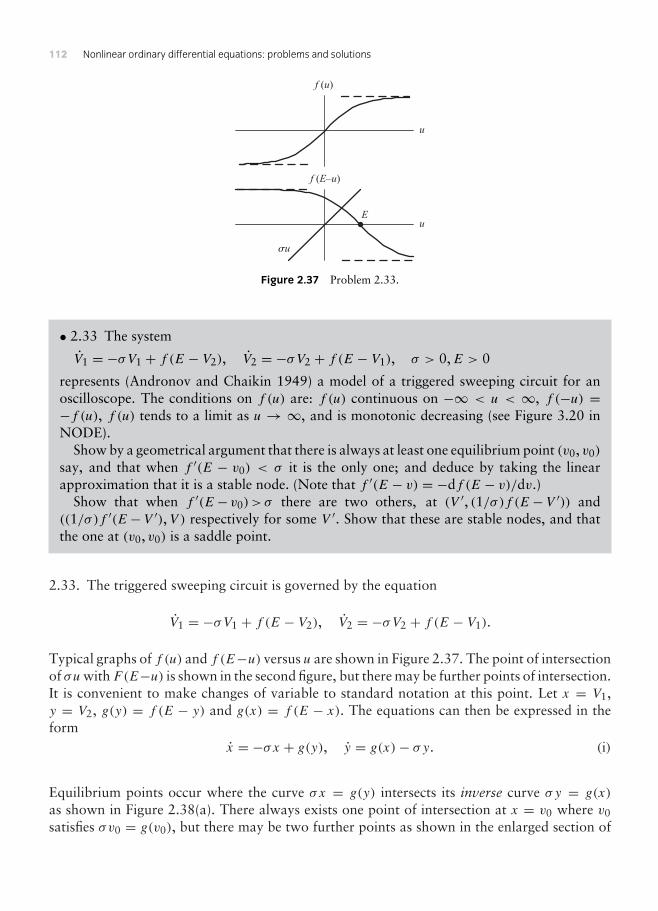
112 Nonlinear ordinary differential equations: problems and solutions
u
f (E–u)
E
su
u
f (u)
Figure 2.37 Problem 2.33.
• 2.33 The system
V1 = −σV1 + f (E − V2), V2 = −σV2 + f (E − V1), σ > 0,E > 0
represents (Andronov and Chaikin 1949) a model of a triggered sweeping circuit for anoscilloscope. The conditions on f (u) are: f (u) continuous on −∞ < u < ∞, f (−u) =−f (u), f (u) tends to a limit as u → ∞, and is monotonic decreasing (see Figure 3.20 inNODE).
Show by a geometrical argument that there is always at least one equilibrium point (v0, v0)
say, and that when f ′(E − v0) < σ it is the only one; and deduce by taking the linearapproximation that it is a stable node. (Note that f ′(E − v) = −df (E − v)/dv.)
Show that when f ′(E− v0)> σ there are two others, at (V ′, (1/σ)f (E−V ′)) and((1/σ)f ′(E−V ′),V ) respectively for some V ′. Show that these are stable nodes, and thatthe one at (v0, v0) is a saddle point.
2.33. The triggered sweeping circuit is governed by the equation
V1 = −σV1 + f (E − V2), V2 = −σV2 + f (E − V1).
Typical graphs of f (u) and f (E−u) versus u are shown in Figure 2.37. The point of intersectionof σuwithF(E−u) is shown in the second figure, but there may be further points of intersection.It is convenient to make changes of variable to standard notation at this point. Let x = V1,y = V2, g(y) = f (E − y) and g(x) = f (E − x). The equations can then be expressed in theform
x = −σx + g(y), y = g(x)− σy. (i)
Equilibrium points occur where the curve σx = g(y) intersects its inverse curve σy = g(x)
as shown in Figure 2.38(a). There always exists one point of intersection at x = v0 where v0satisfies σv0 = g(v0), but there may be two further points as shown in the enlarged section of

2 : Plane autonomous systems and linearization 113
–1 1 2x
–1
1
2y
x = g(y) /s
y = g(x)/s
1x
1y
v2 v0 v1
(b)(a)
Figure 2.38 Problem 2.33: The figures has been drawn with the value σ = 1 and the function g(x) =1.163 tanh[1.2(1 − x)]. The intersections occur at v0 = 0.561, v1 = 0.906 and v2 = 0.130, approximately, asindicated in the enlarged inset shown in (b).
the figure shown in Figure 2.38(b). The latter will occur if the slope of y = g(x)/σ at (v0, v0) isless than −1, since the curves are mutual inverses. Therefore there are three equilibrium pointsif and only if g′(v0) < −σ , and one at x = v0 if g′(v0) > −σ . When there are three such pointsthey are labelled as (v0, v0), (v1, v2) and (v2, v1) as shown in the figure. Since the curves aremutual inverse functions, then σv1 = g(v2) and σv2 = g(v1).
(i) 0 > g′(v0) > −σ . For the only equilibrium point x = v0, let x = v0 + ξ and y = v0 + η.Then the linear approximation of (i) is given by
ξ = −σ(v0 + ξ)+ g(v0 + η) ≈ −σξ + g′(v0)η,
η = g(v0)+ ξ)− σ(v0 + η) ≈ g′(v0)ξ − ση.
The parameters are
p = −2σ < 0, q = σ 2 − g′(v0)2 > 0, = 4g′(v0)
2 > 0.
Therefore (v0, v0) is a stable node.
(ii) g′(v0) < −σ . From (i) the equilibrium point (v0, v0) has the parameter values
p = −2σ < 0, q = σ 2 − g′(v0)2 < 0.
Therefore (v0, v0) is a saddle point.For the point (v1, v2), let x = v1 + ξ and y = v2 + η. Then substitution in (i) leads to
ξ = −σ(v1 + ξ)+ g(v2 + η) ≈ −σξ + g′(v2)η,
η = g(v1)+ ξ)− σ(v2 + η) ≈ g′(v1)ξ −ση.

114 Nonlinear ordinary differential equations: problems and solutions
1x
1
y
Figure 2.39 Problem 2.33: Phase diagram for x = −σx + 1.163 tanh[1.2(1− y)], y = 1.163 tanh[1.2(1− x)] − σywith σ = 1, showing a saddle and two stable nodes.
The parameters of this linear approximation are
p = −2σ < 0, q = σ 2 − g′(v1)g′(v2), = 4g′(v1)g
′(v2) > 0.
Consider the intersection of the curves C1 : y = g(x)/σ and C2 : x = g(y)/σ at x = v1. If theslope of C1 is m1, and of C2 is m2 at x = v1, then m1 > m2 (see Figure 2.38). Therefore, since
m1 = g′(v1)
σand m2 = σ
g′(v2),
it follows that g′(v1)g′(v2) < σ 2 (remember that g′(v1) and g′(v2) are negative which affects
manipulation of the inequalities). Hence for the equilibrium point (v1, v2), q > 0 which meansthat the equilibrium point is a stable node.
A similar argument can be used to show that (v2, v1) is also a node: simply interchange v1and v2 in the analysis above. A phase diagram for case (ii) (three equilibrium points) is shownin Figure 2.39 for the same parameter values as in Figure 2.38.
• 2.34 Investigate the equilibrium points of x = a − x2, y = x − y. Show that the systemhas a saddle and a stable node for a > 0 but no equilibrium points if a < 0. The system issaid to undergo a bifurcation as a increases through a = 0. This bifurcation is an exampleof a saddle-node bifurcation. Draw phase diagrams for a = 1 and a = −1.
2.34. The parameter-dependent system is
x = a − x2, y = x − y.

2 : Plane autonomous systems and linearization 115
Equilibrium points occur where a−x2 = 0 and x−y = 0. If a < 0, then there are no equilibriumpoints. If a > 0, there are equilibrium points at (
√a,√a) and (−√a,−√a).
(a) (√a,√a). Let x = √a + ξ , y = √a + η. Then the linear approximation is
ξ ≈ −2√aξ , η = ξ − η.
The associated parameters are
p = −2√a − 1 < 0, q = 2
√a > 0, = 4
√a + 1 > 0.
Hence (√a,√a) is a stable node.
(b) (−√a,−√a). Let x = −√a + ξ , y = −√a + η. Then the linear approximation is
ξ ≈ 2√aξ , η = ξ − η.
The parameter q is given by q = −2√a < 0, so that (−√a,−√a) is a saddle point.
Some phase paths for the case a = 1 are shown in Figure 2.40.
• 2.35 Figure 2.16 (in NODE) represents a circuit for activating an electric arc Awhich hasthe voltage-current characteristic shown. Show that LI = V −Va(I ), RCV = −RI −V +Ewhere Va(I ) has the general shape shown in Figure 2.16 (in NODE). By forming the linearapproximating equations near the equilibrium points find the conditions on E, L, C, R andV ′a for stable working, assuming that V = E−RI meets the curve V = Va(I )in three pointsof intersection.
–2 –1 1 2x
–2
–1
1
2y
Figure 2.40 Problem 2.34: Phase diagram for x = a − x2, y = x − y for a = 1, showing a stable node at (1, 1) anda saddle point at (−1,−1).

116 Nonlinear ordinary differential equations: problems and solutions
2.35. Consult Figure 2.16 in NODE. For the voltage V , we have on the right- and left-handsides,
V − LdIdt− Va(I ) = 0, (i)
andE − Ri − v = 0. (ii)
For the circuit including the capacitance C and the inductance L,
− 1C
∫(i − I )dt + V = 0, or i = I + C dV
dt. (iii)
Eliminate i between (ii) and (iii) giving
V + 1RC
V = E − RIRC
. (iv)
The required first-order equations are given by (i) and (iv), namely
I = V
L− Va(I )
L, V = − 1
CI − 1
RCV + E
RC. (v)
Let (In,Vn), (n = 1, 2, 3) be the equilibrium points, and consider the perturbations I = In + ξ ,V = Vn + η. Then, from (iv),
ξ = 1L
[Vn − Va(In + ξ)] ≈ − 1LV ′a(In)ξ +
1Lη,
η = − 1C(In + ξ)− 1
RC(Vn + η)+ E
RC= − 1
Cξ − 1
RCη,
where Vn and In satisfy Vn−Va(In) = 0 and −RIn−Vn+E = 0 for each value of n. In generalin the linear approximations the parameters are
p = − 1LV ′a(In)−
1RC
, q = V ′a(In)RCL
+ 1LC
.
• (I1,V1). From Figure 2.41, V ′a(I1) > 0 so that p < 0 and q > 0, which means that theequilibrium is either a stable node or spiral depending on the sign of = p2 − 4q.
• (I2,V2). From Figure 2.41, V ′a(I2) < 0. Stability will depend on the signs of p and q. IfV ′a(I2) < −L, then the equilibrium point is a saddle (and unstable). If Va(I2) < −L/(RC),then p < 0 so that the equilibrium point is an unstable node or spiral. We can combinethese instability conditions into the single condition V ′a(I2) < max(−L,−L/(RC)). IfV ′a(I2) > max(−L,−L/(RC)), then p < 0 and q > 0 which means that (I2,V2) is stable.
• (I3,V3). From Figure 2.41, it can be seen that V ′a(I3) < 0 also. Therefore, the results arethe same as the previous case with I2, V2 replaced by I3, V3.

2 : Plane autonomous systems and linearization 117
I
V
(I3,V3)
(I2,V2)
(I1,V1)
V = Va(I)
V = E – RI
Figure 2.41 Problem 2.35: This figure was plotted using Va(I ) = 0.05 + xe−2.5x and the line V = 0.2 − 0.06I tocreate three points of intersection.
• 2.36 The equation for the current x in the circuit of Figure 2.17(a) (in NODE) is
LCx + RCx + x = I .
Neglect the grid current, and assume that I depends only on the relative grid potentialeg : I = IS (saturation current) for eg > 0 and I = 0 for eg < 0 (see Figure 2.17(b) inNODE). Assume also that the mutual indictance M > 0, so that eg <,> 0 according asx >,< 0. Find the nature of the phase paths. By considering their successive intersectionswith the x axis show that a limit cycle is approached from all initial conditions (assumeR2C < 4L).
2.36. The equation for the current x is
LCx + RCx + x = I ,
where
I =Is x > 00 x < 0
.
The (x, y) phase plane equations with y = x are
x = y, y = −ω2x − 2ky +ω2Is(> 0) y > 00 y < 0
,
where ω2 = 1/(LC) and k = R/(2L).The solutions are (for ω2 > k2, that is, R2C > 4L)
x = Ae−kt cos(t + α) for y < 0,
x = Is + Ae−kt cos(t + α) for y > 0.

118 Nonlinear ordinary differential equations: problems and solutions
x
y
xm xm+1
xm+2
Figure 2.42 Problem 2.36: Three successive intersections xm, xm+1, xm+2 with the x axis.
Consider the sequence of intersections xm, xm+1, xm+2 with the y axis as shown in Figure 2.42.Let t = t0 at x = xm and t = t0 + T , where T = π/, at x = xm+1. Therefore
xm+1 = −e−kT xm.
Similarly
xm+2 = Is − e−kT xm+1 = Is + λxm, (i)
putting λ = e−kT . Let m be an even number, say, 2n− 2. Then iteration of (i) gives
x2n = Is + λ(Is + λ(Is + λ(· · · + λ(Is + λx0)) · · · ))= Is + λIs + · · · + λn−1Is + λnx0
= 1− λn1− λ Is + λ
nx0
→ Is
1− λ
as n→∞ for all x0. Since this limit of x2n exists there must be a limit cycle through x = Is/(1−λ)It cuts the x axis again at x = −λIs/(1− λ).
• 2.37 For the circuit in Figure 2.17(a) (in NODE) assume that the relation between I andeg is as in Figure 2.18 (in NODE); that is I = F(eg + kep), where eg and ep are relativegrid and plate potentials, k > 0 is a constant, and in the neighbourhood of the point ofinflection, f (u) = I0+ au− bu3, where a.0, b > 0. Deduce the equation for x when the DCsource E is set so that the operating point is the point of inflection. (A form of Rayleigh’sequation is obtained, implying an unstable or a stable limit cycle respectively.)

2 : Plane autonomous systems and linearization 119
2.37 As in the previous problem,
LCx + RCx + x = I ,
whereI = I0 + a(eg + kep − E0)− b(eg + kep − E0)
3,
eg = M dxdt
, E − Ldxdt− Rx − ep = 0.
Therefore
eg + kep − E0 = (M − kL)dxdt− kRx + kE − E0 = (M − kL)x − kRx,
when the working point E0 = kE. Finally x satisfies
x + R
Lx + 1
LCx = 1
LC[I0 + a[(M − kL)x − kRx] − b[(M − kL)x − kRx]3].
This can be rearranged in the form
x + Ax + Bx3 + ω2x = D,
where
A = 1LC
[R
L− a(M − kL)
], B = b
LC(M − kL)3, D = I0
LC.
If the right-hand side is reduced to zero by a suitable translation of x, then the result is Rayleigh’sequation (see Example 4.6). It has a stable limit cycle if A < 0 and B > 0, that is, if
R < aL(M − kL) and M > kL.
• 2.38 Figure 2.19(a) (in NODE) represents two identical DC generators connected inparallel, with inductance and resistance L, r. Here R is the resistance of the load. Show thatthe equations for the currents are
Ldi1dt= −(r + R)i1 − Ri2 + E(i1), Ldi2
dt= −Ri1 − (r + R)i2 + E(i2).
Assuming that E(i) has the characteristics indicated by Figure 2.19(b) (in NODE) showthat
(i) when E′(0) < r the state i1 = i2 = 0 is stable and is otherwise unstable;
(ii) when E′(0) < r there is a stable state i1 = −i2 (no current flows to R);
(iii) when E′(0) > r + 2R there is a state with i1 = i2, which is unstable.

120 Nonlinear ordinary differential equations: problems and solutions
2.38. For the upper circuit, through generator E(i1) and resistance R,
E(i1)− Ldi1dt− ri1 − R(i1 + i2) = 0,
and for the lower circuit through the generator E(i2) and resistance R,
E(i2)− Ldi2dt− ri2 − R(i1 + i2) = 0.
These equations can be rearranged into
Ldi1dt= −(r + R)i1 − Ri2 + E(i1),
Ldi2dt= −Ri1 − (r + R)i2 + E(i2).
An equilibrium or steady state occurs when the right-hand sides are zero, or when
E(i1) = (r + R)i1 + Ri2,
E(i2) = Ri1 + (r + R)i2.
Let (i1, i2) = (a, b) be an equilibrium point, and let i1 = a + x, i2 = b + y. Then for small |x|and |y|,
Lx ≈ [−(r + R)+ E′(a)]x − Ry,
Ly ≈ −Rx + [−(r + R)+ E′(b)]y.
The parameters associated with this linear approximation are
p = E′(a)+ E′(b)− 2(r + R), q = [E′(a)− (r + R)][E′(b)− (r + R)] − R2.
(i) The point (0, 0) is always an equilibrium point. At this point
p = 2E′(0)− 2r − 2R, q = (E′(0)− r − R)2 − R2 = (E′(0)− r − 2R)(E′(0)− r).For 0 < E′(0) < r, p < 0 and q > 0 which means that the equilibrium point is stable. Ifr + 2R > E′(0) > r, then q < 0 which implies that the equilibrium point is a saddle point(unstable). If E′(0) > r + 2R, then p > 0 and q > 0 which imply that the equilibrium point iseither an unstable node or unstable spiral.
(ii) Since E(i) is an odd function, the equations for equilibrium are unchanged if i1 is replacedby −i2, and i2 by −i1. Let i1 = −i2 = i0. It follows that (i0,−i0) is an equilibrium state whereE(i0) = ri0. The parameters for the linear approximation are
p = −2(r + R) < 0, q = r2 + 2rR − E′(i0)2 > 0
if E′(0) < r. Hence the equilibrium is a stable node or spiral.

2 : Plane autonomous systems and linearization 121
(iii) If i1 = i2 = i0, say, then both equilibrium equations are the same so that i0 satisfiesE(i0) = (r + 2R)i0. Whether non-zero solutions of this equation exist will depend on the slopeE′(0), which must be less than r + 2R for existence. The parameters in this case are
p = 2[E′(i0)− r − R], q = [E′(i0)− (r + R)]2 − R2 = [E′(i0)− r][E′(i0)− r − 2R].
If r < E′(0) < r + 2R, then p < 0 and q < 0 which implies that the equilibrium point is asaddle point.
• 2.39 Show that the Emden–Fowler equation of astrophysics
(ξ2η′)′ + ξληn = 0
is equivalent to the predator–prey model
x = −x(1+ x + y), y = y(λ+ 1+ nx + y)after the change of variable x = ξη′/η, y = ξλ−1ηn/η′, t = ln |ξ |
2.39. The Emden–Fowler equation is
(ξ2η′)′ + ξληn = 0,
or
2ξη′ + ξ2η′′ + ξληn = 0. (i)
Let
x = ξη′
η, y = ξλ−1ηn
η′, t = ln |ξ |.
Then, since ξ = ξ ,
x = ξ η′
η+ ηη′′ξ
η− ξη′2ξ
η2
= ξη′
η+ ξ2η′′
η− ξ2η′2
η2
= ξη′
η+ 1η[−ξληn − 2ξη′] − ξ2η′2
η2 (using (i))
= −x − x2 − (ξληn−1)
= −x − x2 − xy.

122 Nonlinear ordinary differential equations: problems and solutions
Similarly
y = (λ− 1)ξλ−1ξ ηn
η′+ nξλ−1ηn−1ξ − ξλ−1ηnη′′ξ
η′2
= (λ− 1)ξλ−1ηn
η′+ nξληn−1 + ξλ−1ηn
η′(2ξη′ + ξληn)
= (λ+ 1)y + nxy + y2,
as required.
• 2.40 Show that Blasius’ equation
η′′′ + ηη′′ = 0
is transformed by x = ηη′/η′′, y = η′2/(ηη′′), t = ln |η′| into
x = x(1+ x + y), y = y(2+ x − y).
2.40. The Blasius equation is
η′′′ + ηη′′ = 0, (i)
where η′ = dη/dξ . Let
x = ηη′
η′′, y = η′2
ηη′′, t = ln |η′|, or η′ = et .
Differentiating η′ = et with respect to t , we have
η′′ξ = et = η′, so that ξ = η′
η′′. (ii)
Then
x = η′2ξη′′
+ ηξ − ηη′η′′′ξη′′2
= η′3
η′′2+ ηη′
η′′− ηη′2η′′′
η′′2(using (ii))
= η′3
η′′2+ ηη′
η′′+ η2η′2
η′′2(using (i))
= xy + x + x2 = x(1+ x + y)

2 : Plane autonomous systems and linearization 123
as required. Similarly
y = 2η′ξη− η′3ξη2η′′
− η′2η′′′ξηη′′2
= 2η′2
ηη′′− η′4
η2η′′2− η′3η′′′
ηη′′3(using (ii))
= 2η′2
ηη′′− η′4
η2η′′2+ η′3
η′′2(using (i))
= 2y − y2 + xy = y(2+ x − y).
• 2.41 Consider the family of linear systems
x = X cosα − Y sinα, y = X sinα + Y cosα
where X = ax + by, Y = cx + dy, and a, b, c, d are constants and α is a parameter. Showthat the parameters are
p = (a + d) cosα + (b − c) sinα, q = ad − bc.Deduce that the origin is a saddle point for all α if ad < bc. If a = 2, b = c = d = 1,show that the equilibrium point at the origin passes through the sequence stable node, stablespiral, centre, unstable spiral, unstable node as α varies over range π .
2.41. The linear system is
x = (a cosα − c sinα)x + (b cosα − d sinα)y,y = (a sinα + c cosα)x + (b sinα + d cosα)y.
The parameters associated with the origin of this linear system are
p = (a + d) cosα + (b − c) sinα,
q = (a cosα − c sinα)(b sinα + d cosα)− (b cosα − d sinα)(a sinα + c cosα)
= ad − bc.
If ad − bc < 0, then q < 0, which means that the origin is a saddle point for all α.If a = 2, b = c = d = 1, then p = 3 cosα, q = 1 > 0 and = p2 − 4q = 9 cos2 α − 4.
The different stabilities can be seen most easily by sketching the graphs of p and against αas shown in Figure 2.43. The nature of the equilibrium at the origin changes where either p or changes sign at A, B and C (q > 0 so that a saddle is not possible). The classification is asfollows:
• Interval OA: p > 0, > 0, unstable node.• Point A: p > 0, = 0, degenerate unstable node.• Interval AB: p > 0, < 0, unstable spiral.
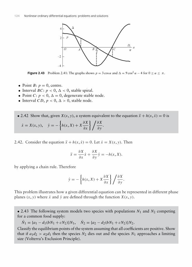
124 Nonlinear ordinary differential equations: problems and solutions
p2
pa
–4
–2
2
4
p
O BD
CA
Figure 2.43 Problem 2.41: The graphs shows p = 3 cosα and = 9 cos2 α − 4 for 0 ≤ α ≤ π .
• Point B: p = 0, centre.• Interval BC: p < 0, < 0, stable spiral.• Point C: p < 0, = 0, degenerate stable node.• Interval CD, p < 0, > 0, stable node.
• 2.42 Show that, given X(x, y), a system equivalent to the equation x + h(x, x) = 0 is
x = X(x, y), y = −h(x,X)+X∂X
∂x
/∂X
∂y.
2.42. Consider the equation x + h(x, x) = 0. Let x = X(x, y). Then
x = ∂X
∂xx + ∂X
∂yy = −h(x,X).
by applying a chain rule. Therefore
y = −h(x,X)+X∂X
∂x
/∂X
∂y.
This problem illustrates how a given differential equation can be represented in different phaseplanes (x, y) where x and y are defined through the function X(x, y).
• 2.43 The following system models two species with populations N1 and N2 competingfor a common food supply:
N1 = a1 − d1(bN1 + cN2)N1, N2 = a2 − d2(bN1 + cN2)N2.
Classify the equilibrium points of the system assuming that all coefficients are positive. Showthat if a1d2 > a2d1 then the species N2 dies out and the species N1 approaches a limitingsize (Volterra’s Exclusion Principle).

2 : Plane autonomous systems and linearization 125
2.43. The two-species model is governed by the equations
N1 = a1 − d1(bN1 + cN2)N1,
N2 = a2 − d2(bN1 + cN2)N2.
Equilibrium occurs where
a1 − d1(bN1 + cN2)N1 = 0, a2 − d2(bN1 + cN2)N2 = 0.
Assume that a1d2 = a2d1 (otherwise there is a line of equilibrium points along bN1 + cN2 =a1/d1). In the (N1,N2) plane, there are three equilibrium points, at
(0, 0), (0, ν2), (ν1, 0),
where ν2 = a2/(cd2) and ν1 = a1/(bd1).
• (0, 0). The linear approximation is
N1 ≈ a1N1, N2 ≈ a2N2.
The parameters are (NODE, Section 2.5)
p = a1 + a2 > 0, q = a1a2 > 0, = (a1 + a2)2 − 4a1a2
= (a1 − a2)2 > 0.
Therefore the origin is an unstable node.• (0, ν2). Let N1 = ξ and N2 = ν2 + η. Then
ξ ≈ a1d2 − a2d1
d2ξ ,
η ≈ −a2b
cξ − a2η.
The parameters are
p = a1d2 − a2d1
d2− a2, q = − (a1d2 − a2d1)a2
d2,
where classification depends on the signs of p and q using the table in Figure 2.10 inSection 2.5 of NODE.
• (ν1, 0). Let N1 = ν1 + ξ and N2 = η. Then
ξ ≈ −a1ξ − ca1
bη.
η ≈ a2d1 − a1d2
d1η.

126 Nonlinear ordinary differential equations: problems and solutions
The parameters are
p = a2d1 − a1d2
d1− a1, q = − (a2d1 − a1d2)a1
d1,
where classification depends on the signs of p and q using the table.
If a1d2 > a2d1, then, for (0, ν2), p > 0 and q < 0 making the point a saddle. Also, for (ν1, 0),p < 0 and q > 0 implying that the equilibrium point is stable, either a node or spiral. This isthe only stable point so that eventually N2 → 0 and N1 → ν1.
• 2.44 Show that the system
x = X(x, y) = −x + y, y = Y (x, y) = 4x2
1+ 3x2 − y
has three equilibrium points, at (0, 0), (13 , 1
3 ) and (1, 1). Classify each equilibrium point.Sketch the isoclines X(x, y) = 0 and Y (x, y) = 0, and indicate the regions where dy/dx ispositive, and where dy/dx is negative. Sketch the phase diagram of the system.
2.44. The system is
x = X(x, y) = −x + y, y = Y (x, y) = 4x2
1+ 3x2 − y.
Equilibrium occurs where
x = y,4x2
1+ 3x2 = y.
Eliminate y leaving
x = 4x2
1+ 3x2 , or 3x3 − 4x2 + x = 0.
Therefore x = 0, 1, 13 and the equilibrium points are (0, 0), (1
3 , 13 ) and (1, 1).
• Equilibrium point (0, 0). The linear approximation is
x = −x + y, y ≈ −y.
The associated parameters are
p = −2 < 0, q = 1 > 0, = p2 − 4q = 0.
Hence (0, 0) is a degenerate stable node.

2 : Plane autonomous systems and linearization 127
1
1
X = 0
Y = 0
O
A
B
1x
1
y
Figure 2.44 Problem 2.44: The phase diagram for x = −x + y, y = [4x2/(1 + 3x2)] − y. Equilibrium points lie atO : (0, 0), A : ( 1
3 , 13 ) and B : (1, 1). The shaded regions, bounded by X(x, y) = 0 and Y (x, y) = 0 indicate where
dy/dx > 0.
• Equilibrium point (13 , 1
3 ). Let x = 13 + ξ and y = 1
3 + η. Then for small |ξ | and |η|, thelinear approximation is
ξ = −ξ + η, η = 4((1/3)+ ξ)21+ 3((1/3)+ ξ)2 −
13 − η ≈ 3
2ξ − η.
The associated parameters are
p = −2, q = 1− 32 = −1
2 .
Therefore (13 , 1
3 ) is a saddle point.
• Equilibrium point (1, 1). Let x = 1+ ξ and y = 1+ η. Then the linear approximation is
ξ = −ξ + η, η = 4(1+ ξ)21+ 3(1+ ξ)2 ≈
12ξ − η.
The parameters are
p = −2 < 0, q = 1− 12 = 1
2 > 0, = 4− 14 = 15
16 > 0.
Therefore (1, 1) is a stable node.
The phase diagram is shown in Figure 2.44 together with the isoclines X(x, y) = 0 andY (x, y) = 0.
• 2.45 Show that the systems (A) x = P(x, y), y = Q(x, y) and (B) x = Q(x, y), y = P(x, y)have the same equilibrium points. Suppose that system (A) has three equilibrium pointswhich, according to their linear approximations are, (a) a stable spiral, (b) an unstablenode, (c) a saddle point. To what extent can the equilibrium points in (B) be classified fromthis information?

128 Nonlinear ordinary differential equations: problems and solutions
2.45. Comparison is to be made between the systems
(A) x = P(x, y), y = Q(x, y)
and
(B) y = Q(x, y), y = P(x, y).
Assume that in a neighbourhood of an equilibrium point
P(x, y) ≈ ax + by, Q(x, y) ≈ cx + dy.
Then the linear approximation for system (A) is
x = ax + by, y = cx + dy,
and for system (B),x = cx + dy, y = ax + by.
Hence the parameters classifying equilibrium points for (A) are
pA = a + d, qA = ad − bc, A = (a + d)2 − 4(ad − bc) = (a − d)2 + 4bc,
and for (B) are
pB = b + c, qB = bc − ad, B = (b + c)2 − 4(bc − ad) = (b − c)2 + 4ad.
(a) A has a stable spiral, which means that
pA = a + d < 0, qA = ad − bc > 0, A = (a − d)2 + 4bc < 0.
It can be seen that qB = bc− ad < 0. Therefore the corresponding equilibrium point for (B) isa saddle.
(b) A has a an unstable node, which requires
pA = a + d > 0, qA = bc − ad > 0 and A = (a − d)2 + 4bc > 0.
As in (a), qB = bc − ad < 0. Hence the equilibrium point in (B) is also a saddle.
(c) (A) has a saddle. Hence qA = ad − bc < 0. It follows that
pB = b + c, qB = bc − ad > 0, B = (b + c)2 − 4(bc − ad) = (b − c)2 + 4ad.

2 : Plane autonomous systems and linearization 129
All we can say generally is that the equilibrium point is a node or a spiral, where stability willdepend on the sign of pA = b + c.
• 2.46 The system defined by the equations
x = a + x2y − (1+ b)x, y = bx − yx2, (a = 0, b = 0)
is known as the Brusselator and arises in a mathematical model of a chemical reaction (seeJackson (1990)). Show that the system has one equilibrium point at (a, b/a). Classify theequilibrium point in each of the following cases:
(a) a = 1, b = 2;
(b) a = 12 , b = 1
4 .
In case (b) draw the isoclines of zero and infinite slope in the phase diagram. Hence sketchthe phase diagram.
2.46. The system isx = a + x2y − (1+ b)x, y = bx − yx2.
Equilibrium occurs where
a + x2y − (1+ b)x = 0, x(b − xy) = 0,
which have just one solution x = a, y = b/a.Let x = a + ξ , y = (b/a)+ η. Then
ξ = a + (a + ξ)2(b
a+ η
)− (1+ b)(a + ξ) ≈ (b − 1)ξ + a2η,
and
η = (a + ξ)[b − (a + ξ)
(b
a+ η
)]≈ bξ − a2η
The parameters associated with the linear approximation are
p = b − 1− a2, q = a2(1− 2b), = (b − 1)2 + a2(6b − 2+ a2).
(a) Case a = 1, b = 2. The equilibrium point is at (1, 2). The parameters are p = 0,q = −3 < 0. Therefore (1, 2) is a saddle point.
(b) Case a = 12 , b = 1
4 . The equilibrium point is at (12 , 1
2 ). The parameters are p = −1 < 0,q = 1
8 > 0, = 12 > 0. Therefore (1
2 , 12 ) is also a stable node.The phase diagram for case (b)
is shown in Figure 2.45.

130 Nonlinear ordinary differential equations: problems and solutions
–1 1 2x
–1
1
2y
Figure 2.45 Problem 2.46: Phase diagram for a = 12 , b = 1
4 showing a stable node at ( 12 , 1
2 ). The dashed curveindicates the isocline with infinite slope and the grey curves the isoclines with zero slope (including the y axis).
• 2.47 A Volterra model for the population size p(t) of a species is, in reduced form,
κdpdt= p − p2 − p
∫ t
0p(s)ds, p(0) = p0,
where the integral term represents a toxicity accumulation term (see Small (1989)). Letx = lnp, and show that x satisfies
κx + exx + ex = 0.
Put y = x, and show that the system is also equivalent to
y = −(y + 1)p/κ, p = yp.
Sketch the phase diagram in the (y,p) plane. Also find the exact equation of the phase paths.
2.47. The Volterra model for the population p(t) satisfies
κdpdt= p − p2 − p
∫ t
0p(s)ds, p(0) = p0. (i)
Differentiate equation (i) with respect to t :
κp = p − 2pp − p∫ t
0p(s)ds − p2
= p − 2pp − p
p[−κp + p − p2] − p2, (using (i))
= −pp + κ p2
p− p2.
Let p = ex so that p = exx and p = exx + exx2. Then the population equation becomes
κ(exx + exx2) = −e2xx + κexx2 − e2x ,

2 : Plane autonomous systems and linearization 131
–1 1 2y
1
2
p
Figure 2.46 Problem 2.47: Phase diagram for the Volterra model with κ = 1.
or
κx + exx + ex = 0, (ii)
as required.Let y = x. Then p = exx = py. Also
y = x = −1κ(exx + ex) = −1
κ(y + 1)p,
using (ii). Equilibrium occurs for all points on the axis p = 0 (for the population model p ≥ 0).The differential equation for the phase paths in the (y,p) plane is
dydp
= −y + 1κy
.
For t = 0, p(0) = p(0) − p(0)2 < 0 assuming that p(0) > 1. This is a separable equationwith general solution
κ
∫y
y + 1dy = −
∫dp = −p + C,
or
κ(y − ln |y + 1|) = −p + C.
A phase diagram for the model is shown in Figure 2.46 with κ = 1. In fact this includes all non-zero parameter values for κ, since κ can be eliminated from the from the first-order equationsby the transformation p→ pκ.

This page intentionally left blank

3Geometrical aspects ofplane autonomous systems
• 3.1 By considering the variation of path direction on closed curves round the equilibriumpoints, find the index in each case of Figure 3.29 (in NODE)
3.1. (a) Surround the equilibrium point by a closed curve (see Figure 3.1). Take any pointP on , and draw a vector S at P tangential to the phase path at P . Let φ be the anglebetween a fixed direction and S measured counterclockwise as shown. As P makes one coun-terclockwise circuit of , determine how the angle φ changes as the direction of S changes.Any change will be a multiple of 2π . In this example φ returns to its original value. Hence theindex I = 0.
Apply the same method to each of the remaining figures. The indices are
(b) I = 0.
(c) I = 1.
(d) I = 1.
(e) I = −2.
P
S
fΓ
Figure 3.1 Problem 3.1(a)

134 Nonlinear ordinary differential equations: problems and solutions
• 3.2 The motion of a damped pendulum is described by the equations
θ = ω, ω = −kω − ν2 sin θ ,
where k(> 0) and ν are constants. Find the indices of all equilibrium states.
3.2. The damped pendulum has the equation
θ = ω, ω = −kω − ν2 sin θ .
Equilibrium occurs where ω = 0 and sin θ = 0, that is, at (nπ , 0), (n = 0,±1,±2, . . . ) in the(θ ,ω) phase plane.
Near the origin,θ = ω, ω ≈ −ν2θ − kω.
The parameters associated with the linear approximation (see Section 2.5) are
p = −k < 0, q = ν2 > 0, = k2 − 4ν2.
Hence the equilibrium point is either a stable node or a stable spiral depending on the sign of.In both cases, however, the index I = 1. By the 2π periodicity in θ of the differential equation,the indices of all the equilibrium points (2πn, 0), (n = 0,±1,±2, . . . ) also have index I = 1.
Near θ = π , let θ = π + ξ . Then
ξ = ω, ω = −kω − ν2 sin(π + ξ) ≈ −kω + ν2ξ .
Therefore q = −ν2, that is, the equilibrium point is a saddle point with index I = −1. Similarlyall the points ((2n+ 1)π , 0), (n = 0,±1,±2, . . . ) are saddle points each with index I = −1.
• 3.3 Find the index of the equilibrium points of the following systems: (i) x = 2xy,y = 3x2 − y2; (ii) x = y2 − x4, y = x3y; (iii) x = x − y, y = x − y2.
3.3. (i) The systemx = 2xy, y = 3x2 − y2
has one equilibrium point, at the origin. Let the curve surrounding the origin be the ellipsex = cos θ , y = √3 sin θ for 0 ≤ θ < 2π . Then
X(x, y) = 2xy = 2√
3 cos θ sin θ = √3 sin 2θ ,
Y (x, y) = 3x2 − y2 = 3(cos2 θ − sin2 θ) = 3 cos 2θ .

3 : Geometrical aspects of plane autonomous systems 135
x
y
X > 0, Y > 0
X < 0, Y > 0
X < 0, Y < 0
X > 0, Y < 0 X > 0, Y > 0
X < 0, Y > 0
X > 0, Y < 0
X < 0, Y < 0
Y = 0
Y = 0
X = 0
X = 0
A
B
C
D
Γ
Figure 3.2 Problem 3.3(b)
Then, on ,
tanφ = Y (x, y)X(x, y)
= 3 cos 2θ√3 sin 2θ
= √3 cot 2θ = √3 tan[12π − 2θ ].
As θ increases from 0 to 2π , φ decreases 0 to −4π . Hence I = −2.(ii) The system
x = y2 − x4, y = x3y
has one equilibrium point, at the origin. Let be a circle centred at the origin. Using the methodof Theorem 3.3, draw the isoclines X(x, y) = 0, that is, y = ±x2, and Y (x, y) = 0, that is, theaxes x = 0 and y = 0, in the phase plane, and mark the regions where X and Y are positiveand negative as shown in Figure 3.2. The circle cuts the lines Y (x, y) = 0 at the points A, B,C and D. According to Theorem 3.3 we list the sign changes of tanφ = Y/X at these pointson a counterclockwise circuit of . The signs of X and Y shown in the figure can be used todetermine the sign changes:
zero of Y (x, y) A B C D
sign change in tanφ +/− +/− +/− +/−Hence there are P = 4 changes from + to −, and Q = 0 changes from − to +. The index is
given by I = 12 (P −Q) = 2.
(iii) The system
x = x − y, y = x − y2

136 Nonlinear ordinary differential equations: problems and solutions
–1 1 2x
–1
1
y
X = 0
X = 0
Y = 0
A
B
C
D
X > 0, Y < 0
X < 0, Y < 0
X < 0, Y > 0
X > 0, Y >0
X > 0, Y < 0
Γ2
Γ1
Figure 3.3 Problem 3.3(c)
has two equilibrium points, at (0, 0) and (1, 1). The isoclinesX(x, y) = x−y = 0 and Y (x, y) =x − y2 = 0 are shown in Figure 3.3. Surround (0, 0) and (1, 1) by circles 1 and 2 as shown:(1, 1) should be outside 1 and (0, 0) outside 2. Let 1 cut x = y2 at A and B, and 2 cutx = y2 at C and D. The sign changes in tanφ = Y/X on a counterclockwise circuit of 1 are
zero of Y (x, y) A B
sign change in tanφ −/+ −/+Hence P = 2 and Q = 0 so that at (0, 0) the index is I = 1
2 (P −Q) = 1.For a counterclockwise circuit of 2,
zero of Y (x, y) C D
sign change in tanφ +/− +/−Hence P = 0 and Q = 2 so that at (1, 1) the index is I = 1
2 (P −Q) = −1.For the origin use result (3.8) with the curve given parametrically by x = r cos t , y = r sin t
(0 ≤ t < 2π) in (iii). Then, on ,
X(x, y) = x − y = r(cos t − sin t), Y (x, y) = r cos t − r2 sin2 t .
Therefore
I= 12π
∮
XdY − YdXX2 + Y 2
= 12π
∫ 2π
0
X(dY/dt)− Y (dX/dt)X2 + Y 2 dt

3 : Geometrical aspects of plane autonomous systems 137
= 12π
∫ 2π
0
(cos t − sin t)(− sin t − 2r sin t cos t)+ (cos t − r sin2 t)(sin t + cos t)
(cos t − sin t)2 + (cos t − r sin2t )2dt
= 12π
∫ 2π
0
1− r sin t(cos2 t + 1− sin t cos t)
(cos t − sin t)2 + (cos t − r sin2 t)2dt .
Therefore, if 0 < r < 1, surrounds only the origin for which I = 1, whilst for r > 1, surrounds both equilibrium points for which I = 0; this is the sum of the indices at (0, 0)and (1, 1).
• 3.4 For the linear system x = ax + by, y = cx + dy, where ad − bc = 0, obtain the indexat the origin by evaluating
I =∫ s1
s0
XY ′ − YX′X2 + Y 2 ds,
showing that it is equal to sgn (ad−bc). (Hint: choose to be the ellipse (ax+by)2+ (cx+dy)2 = 1.)
3.4. The linear system is
x = ax + by, y = cx + dy, (ad − bc = 0).
Let be the ellipse
(ax + by)2 + (cx + dy)2 = 1,
which can be represented parametrically by
X(x, y) = ax + by = cos θ , Y (x, y) = cx + dy = sin θ ,
where 0 ≤ θ < 2π . By solving these equations we obtain
x = d cos θ − b sin θad − bc , y = −c cos θ + a sin θ
ad − bc ,
since ad−bc = 0. As θ increases, the ellipse is tracked in a counterclockwise sense if ad−bc > 0and clockwise if ad − bc < 0. From (3.7), since X = ax + by and Y = cx + dy, but taking

138 Nonlinear ordinary differential equations: problems and solutions
account that must be traced anticlockwise
I = 12π
∫ s1
s0
XY ′ − YX′X2 + Y 2 ds
= sgn (ad − bc)2π
∫ 2π
0
X(dY/dθ)− Y (dX/dθ)X2 + Y 2 dθ
= sgn (ad − bc)2π
∫ 2π
0
cos θ(cos θ)− sin θ(− cos θ)
cos2 θ + sin2 θdθ
= sgn (ad − bc)2π
∫ 2π
0dθ = sgn (ad − bc).
• 3.5 The equation of motion of a bar restrained by springs (see Figure 3.30 in NODE) andattracted by a parallel current-carrying conductor is
x + c(x − λ
a − x)= 0,
where c (the stiffness of the spring), a and λ are positive constants. Sketch the phase pathsfor −x0 < x < a, where x0 is the unstretched length of each spring, and find the indices ofthe equilibrium points for all λ > 0.
3.5. The equation of motion of the bar is
x + c[x − λ
a − x]= 0. (i)
Equilibrium occurs where
x(a − x)− λ = 0, or x2 − ax + λ = 0. (ii)
If λ > 14a
2, there is no equilibrium state. A typical phase diagram is shown in Figure 3.4.If λ < 1
4a2, then the solutions of (ii) are given by
x = 12 [a ±
√(a2 − 4λ)].
Both these solutions are positive. Denote them by x1 and x2. Let x = x1 + ξ . Then eqn (i)becomes
ξ + c[x1 + ξ − λ
a − x1 − ξ]= 0,

3 : Geometrical aspects of plane autonomous systems 139
with linearized approximation
ξ + c[1− λ
(a − x1)2
]ξ = 0.
Therefore the equilibrium point (x1, 0) is a centre if λ < (a − x1)2, making the coefficient of
ξ positive, and a saddle point if λ > (a − x1)2, making it negative. Substituting for x1 these
inequalities becomeλ < 1
4 [a −√(a2 − 4λ)]2 for a centre,
andλ > 1
4 [a −√(a2 − 4λ)]2 for a saddle,
However, it can be shown that the first inequality (the centre) is not consistent with λ < 14a
2,by considering the sign of
λ− 14 [a −
√(a2 − 4λ)]2.
Hence (x1, 0) is a saddle.By a similar argument the linearization near x = x2 leads to the equation
ξ + c[1− λ
(a − x2)2
]ξ = 0.
In this case the critical relation between λ and a is
λ = (a − x2)2, or λ = 1
4 (a +√(a2 − 4λ)),
but since λ < 14a
2 this equilibrium point is a centre. Typical phase diagrams are shown inFigures 3.4 and 3.5.
The index of x1 (the saddle) is −1, and the index of x2 (the centre) is +1.
– 1 1x
y
a
–x0
S–1
1
Figure 3.4 Problem 3.5: The phase diagram for the bar with the parameter values λ = 0.5, a = 1, x0 = 1, c = 1.

140 Nonlinear ordinary differential equations: problems and solutions
–1 1x
– 1
1y
a
–x0
x1x2
Figure 3.5 Problem 3.5: The phase diagram for the bar with the parameter values λ = 0.15, a = 1, x0 = 1, c = 1.
• 3.6 Show that the equation
x − ε(1− x2 − x2)x + x = 0
has an equilibrium point of index 1 at the origin of the phase plane x, y with x = y. (Italso has a limit cycle, x = cos t .) Use NODE, eqn (3.7)(see Problem 3.4), with a circle ofradius a to show that, for all a,∫ 2π
0
dθ
1− 2ε(1− a2) sin θ cos θ + ε2(1− a2)2 sin2 θ= 2π .
3.6. The equationx − ε(1− x2 − x2)x + x = 0
has a single equilibrium point, at the origin. Consider first the special case where is givenparametrically by x = cos θ , y = sin θ . Then
X(x, y) = y = sin θ , Y (x, y) = −x + ε(1− x2 − y2)y = − cos θ ,
on . By NODE, eqn (3.8) in the text, the index of the origin is given by
I = [φ] = 12π
∫ 2π
0
X(dY/dθ)− Y (dX/dθ)X2 + Y 2 dθ
= 12π
∫ 2π
0
sin θ(sin θ)+ cos θ(cos θ)
sin2 θ + cos2 θdθ
= 12π
∫ 2π
0dθ = 1.

3 : Geometrical aspects of plane autonomous systems 141
The system has only one equilibrium point, at the origin. Hence for any simple closed curve surrounding the origin, the change in φ in a counterclockwise circuit must be 2π . In particularfor the curve x = a cos θ , y = a sin θ (a > 0),
2π =∫ 2π
0
a sin θ[a sin θ + ε(1− a2)a cos θ ] − [−a cos θ + ε(1− a2)a sin θ ]a cos θ
a2 sin2 θ + [−a cos θ + ε(1− a2)a sin θ ]2 dθ ,
=∫ 2π
0
dθ
1− 2ε(1− a2) sin θ cos θ + ε2(1− a2)2 sin2 θ
• 3.7 A limit cycle encloses N nodes, F spirals, C centres, and S saddle points only, all oflinear type. Show that N + F + C − S = 1.
3.7. We can let the chosen curve be the limit cycle. Taken in either sense the index I = 1.By Theorem 3.2, the sum of the indices of the equilibrium points within must be 1. Theindices of a linear node, spiral and centre are all 1, whilst the index of the linear saddle is−1. If there are N nodes, F spirals and C centres, then their contribution to the index is(N + F + C) × 1 = N + F + C. If there are S saddles then their contribution is −S. HenceN + F + C − S = 1.
• 3.8 Given the systemx = X(x, y) cosα − Y (x, y) sinα, y = X(x, y) sinα + Y (x, y) cosα,
where α is a parameter, prove that the index of a simple closed curve which does not meetan equilibrium point is independent of α (see Problem 2.41).
3.8. Compare the two systems
x = X(x, y), y = Y (x, y), (A)
andx = P(x, y) = X(x, y) cosα − Y (x, y) sinαy = Q(x, y) = X(x, y) sinα + Y (x, y) cosα
(B)
The systems (A) and (B) have the same equilibrium points, which satisfy X(x, y) = 0 andY (x, y) = 0. Let be the simple closed curve for both systems. In complex terms
X + iY = (P + iQ)eiα,
so that|X + iY | = |P + iQ|, arg(X + iY ) = arg(P + iQ)+ α.

142 Nonlinear ordinary differential equations: problems and solutions
Hence the vector (P ,Q) is the vector (X,Y ) rotated through−α at each point in the phase plane.Hence the index for with (P ,Q) is the same as that of (X,Y ) and this is independent of α.
• 3.9 Suppose that the system x = X(x) has a finite number of equilibrium points, each ofwhich is either a node, a centre, a spiral or a saddle point, of the elementary types discussedin NODE, Section 2.5, and assume that I∞ = 0. Show that the total number of nodes,centres and spirals is equal to the total number of saddle points plus two.
3.9. According to the Corollary to Theorem 3.4, the sum of all the indices including the pointat infinity I∞ is 2, that is, if the indices of the equilibrium points are Ii , (i = 1, 2, . . ., n), then
I∞ +n∑i=1
Ii = 2.
Let there be a total of r centres, nodes and spirals each of which will have index 1, and ssaddles each of which will have index −1, where r + s = n. Since we are given that I∞ = 0,then r − s = 2 as required.
• 3.10 Obtain differential equations describing the behaviour of the linear system, x =ax + by, y = cx + dy, at infinity. Sketch the phase diagram, and analyse the systemx = 2x − y, y = 3x − 2y near the horizon.
3.10. In the equations
x = ax + by, y = cx + dy
let (see NODE, Section 3.2)
x1 = x
x2 + y2 , y1 = − y
x2 + y2 .
With x1 = x/(x2 + y2), y1 = −y/(x2 + y2) and z1 = x1 + iy1, the transformed system is givenby NODE, (3.11)
dz1
dt= −z2
1(X + iY )
= −(x1 + iy1)2[ax + by + i(cx + dy)]
= −(x21 − y2
1 + 2ix1y1)[ax1 − by1 + i(cx1 − dy1)]/r21

3 : Geometrical aspects of plane autonomous systems 143
where r21 = x2
1 + y21 . Therefore, by equating real and imaginary parts of this equation,
x1 = [(y21 − x2
1)(ax1 − by1)+ 2x1y1(cx1 − dy1)]/r21 , (i)
y1 = [−2x1y1(ax1 − by1)+ (y21 − x2
1)(cx1 − dy1)]/r21 . (ii)
For the system x = 2x − y, y = 3x − 2y, the coefficients are a = 2, b = −1, c = 3, d = −2.The origin is a centre with index 1. Hence (i) and (ii) become
x1 = [(y21 − x2
1)(2x1 + y1)+ 2x1y1(3x1 + 2y1)]/r21
= (−2x31 + 5x2
1y1 + 6x1y21 + y3
1)/r21 ,
y1 = [−2x1y1(2x1 + y1)+ (y21 − x2
1)(3x1 + 2y1)]/r21
= (−3x31 − 6x2
1y1 + x1y21 + 2y3
1)/r21
The origin in this system is a singular point since x1 and y1 are not defined at (0, 0). However,we can define a phase diagram through the equation
dy1
dx1= y1
x1= −3x3
1 − 6x21y1 + x1y
21 + 2y3
1
−2x31 + 5x2
1y1 + 6x1y21 + y3
1
.
The origin is a higher-order equilibrium point of the equivalent equations
u = −2u3 + 5u2v + 6uv2 + v3,
v = −3u3 − 6u2v + uv2 + 2v3,
in the (u, v) plane: the phase paths will be identical in the (x1, y1) and (u, v) planes.We shall try to find any separatrices by putting v = ku. Then
dvdu= k = −3− 6k + k2 + 2k3
−2+ 5k + 6k2 + k3 ,
or
k4 + 4k3 + 4k2 + 4k + 3 = 0, or (k + 1)(k + 3)(k2 + 1) = 0.
The quartic has two real solutions k = −1 and k = −3. Computed phase paths in the neigh-bourhood of the origin are shown in Figure 3.6. A counterclockwise circuit of in the figureindicates the the point at infinity has an index of 3. Since the saddle at the origin has index −1,the sum of the indices is 2 which confirms the Corollary to Theorem 3.4.

144 Nonlinear ordinary differential equations: problems and solutions
–0.5 0.5x1
y1
–0.5
0.5Γ
Figure 3.6 Problem 3.10:
• 3.11 A certain system is known to have exactly two equilibrium points, both saddlepoints. Sketch phase diagrams in which
(i) a separatrix connects the saddle points,
(ii) no separatrix connects them.
For example, the system x = 1−x2, y = xy has a saddle connection joining saddle pointsat (±1, 0). The perturbed system x = 1− x2, y = xy− εx2 for 0 < ε 1 breaks the saddleconnection (heteroclinic bifurcation).
3.11. Figure 3.28 (in NODE) shows examples of separatrices which connect two saddle pointsand separatrices which do not. A possible system to illustrate two saddles is
x = 1− x2, y = xy.
Some phase paths for the system are shown in Figure 3.7: the saddles are at (±1, 0) and theseare the only equilibrium points.
A perturbation of this system can break the link between the saddle points. Consider theequations
x = 1− x2, y = xy + εx2,
in which ε is a small parameter. With ε = 0.2, the system has saddle equilibrium points at(1,−0.2) and (−1, 0.2). The separatrices only are shown in Figure 3.8.

3 : Geometrical aspects of plane autonomous systems 145
x
y
Figure 3.7 Problem 3.11: Phase paths for the system x = 1− x2, y = xy.
x
y
Figure 3.8 Problem 3.11: x = 1− x2, y = xy + εx2 showing only the separatrices, in the case ε = 0.2.
• 3.12 Deduce the index at infinity for the system x = x − y, y = x − y2 by calculating theindices of the equilibrium points.
3.12. The system x = x−y, y = x−y2 has equilibrium points where x−y = 0 and x−y2 = 0.There are two such points, at (0, 0) and (1, 1). Their types are as follows:
• (0, 0). The linear approximations are x = x − y, y ≈ x. The associated parameters arep = 1 > 0, q = 1 > 0, = p2 − 4q = 1− 4 = −3 < 0. Hence from Section 2.5, Hence(0, 0) is an unstable spiral with index I1 = 1.
• (1, 1). Let x = 1 + ξ and y = 1 + η. Then the linear approximations are ξ = ξ − η,η = 1+ξ−(1+η)2 ≈ ξ−2η. The parameters arep = 1−2 = −1 < 0, q = −2+1 = −1 < 0which imply that (1, 1) is a saddle point with index I2 = −1.
By Theorem 3.4, I∞ = 2− I1 − I2 = 2− 1+ 1 = 2.
• 3.13 Use the geometrical picture of the field (X,Y ), in the neighbourhood of an ordinarypoint (i.e. not an equilibrium point) to confirm Theorem 3.1.

146 Nonlinear ordinary differential equations: problems and solutions
(X,Y)
Pf
Γ
Figure 3.9 Problem 3.13:
3.13. Figure 3.9 shows on ordinary point P of a phase diagram. Surround P by a closed curve (usually a circle centred at P ) so that there are no equilibrium points in or on . Since xand y are continuous and xP = 0, yP (their values at P ), there exists a neighbourhood of Pin which x and y retain the same signs as xP and yP respectively. Assume that is in thisneighbourhood. Then the direction of the vector (X,Y ) points into the same quadrant at everypoint of , which establishes the result that I = 0.
• 3.14 Suppose that, for two plane systems x1 = X1(x1), x2 = X2(x2), and for a givenclosed curve , there is no point on at which X1 and X2 are opposite in direction. Showthat the index of is the same for both systems.
The system x= y, y= x has a saddle point at the origin. Show that the index of the originfor the system x= y + cx2y, y= x − cy2x is likewise −1.
3.14. Consider the two plane systems x1 = X1(x1), x2 = X2(x2). Let φ(s) be the angle betweenX2 and a fixed direction, and let θ(s) be the angle between X1 and X2 (see Figure 3.10), wheres (α ≤ s < β), is the curve parameter for one circuit of . Since X1 and X2 are never oppositeto each other, that is, −π < θ < π , then θ(α) = θ(β). Then
I(X1) = 12π[θ(s)+ φ(s)]βα
= 12π[θ(s)]βα + [φ(s)]βα
= 12πθ(β)− θ(α)+ φ(β)− φ(α)
= 12π[φ(s)]βα = I(X2),
as required.

3 : Geometrical aspects of plane autonomous systems 147
X1
X2
f
u
Γ
Figure 3.10 Problem 3.14:
The system x = y, y = x has a saddle point at the origin with index −1. The perturbedsystem is x = y + cx2y, y = x − cxy2 which also has just one equilibrium point, at theorigin. Let
X1 = (y, x), X2 = (y + cx2y, x − cxy2).
Let be a circle centre the origin with radius r. On the angle θ between the vectors X1 andX2 is given by
cos θ = X1 ·X2
|X1||X2|
= y(y + cx2y)+ x(x − cxy2)√(x2 + y2)
√[(x − cxy2)2 + (y + cx2y)2]
= r2
r√[r2 + c2r2x2y2]
= 1√[1+ c2x2y2] ,
where r = √(x2 + y2). It follows that cos θ > 0 for all c so that cos θ can never equal −1, thatis, θ can never be −π on . By the first part of the problem, the index of the perturbed systemmust also be −1.
• 3.15 Use Problem 3.14 to show that the index of the equilibrium point x = 0, x = 0 forthe equation x+ sin x = 0 on the usual phase plane has index 1, by comparing the equationx + x = 0.

148 Nonlinear ordinary differential equations: problems and solutions
3.15. The systems x + x = 0 and x + sin x = 0 both have an equilibrium point at the origin,but the second equation will have further equilibrium points at x = nπ , (n = ±1,±2, . . . ).Let be a circle of radius a < π , centre the origin, so that the only equilibrium point inside is the origin. Let be described parametrically by x = a cos θ , y = a sin θ , (0 < θ ≤ 2π). Inthe notation of Problem 3.14, let
X1 = (y,−x), X2 = (y,− sin x).
Then, on ,
X1 = (a sin θ ,−a cos θ), X2 = (a sin θ ,− sin(a cos θ)).
Since the vectors X1 and X2 have the same first component for all θ , they can never be inopposition. Hence, by Problem 3.14, the origin for both systems must have the same index.With x = y, the origin of the system x+ x = 0 is a centre with index 1. Hence the other systemmust have the same index.
• 3.16 The system
x = ax + by + P(x, y), y = cx + dy +Q(x, y)
has an isolated equilibrium point at (0, 0), and P(x, y)=O(r2), Q(x, y)=O(r2) as r→0,where r2= x2+ y2. Assuming that ad − bc =0, show that the origin has the same index asits linear approximation.
3.16. The system
x = ax + by + P(x, y), y = cx + dy +Q(x, y)
has an isolated equilibrium point at the origin. Let
X1 = (ax + by, cx + dy), X2 = X1 + P,
where P = (P (x, y),Q(x, y)). Also let be the circle of radius ρ centred at the origin. Let θ bethe smaller angle between X1 and X2, then
cos θ = X1 ·X2
|X1||X2| =|X1|2 + P ·X1
|X1||X2| .
Since |X1| = O(ρ) and |X2| = O(ρ), then
P ·X1 = O(ρ3).
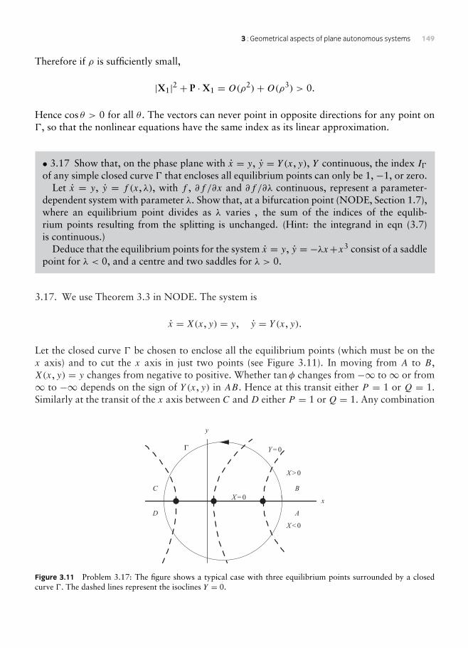
3 : Geometrical aspects of plane autonomous systems 149
Therefore if ρ is sufficiently small,
|X1|2 + P ·X1 = O(ρ2)+O(ρ3) > 0.
Hence cos θ > 0 for all θ . The vectors can never point in opposite directions for any point on, so that the nonlinear equations have the same index as its linear approximation.
• 3.17 Show that, on the phase plane with x = y, y = Y (x, y), Y continuous, the index Iof any simple closed curve that encloses all equilibrium points can only be 1, −1, or zero.
Let x = y, y = f (x, λ), with f , ∂f /∂x and ∂f /∂λ continuous, represent a parameter-dependent system with parameter λ. Show that, at a bifurcation point (NODE, Section 1.7),where an equilibrium point divides as λ varies , the sum of the indices of the equlib-rium points resulting from the splitting is unchanged. (Hint: the integrand in eqn (3.7)is continuous.)
Deduce that the equilibrium points for the system x = y, y = −λx+x3 consist of a saddlepoint for λ < 0, and a centre and two saddles for λ > 0.
3.17. We use Theorem 3.3 in NODE. The system is
x = X(x, y) = y, y = Y (x, y).
Let the closed curve be chosen to enclose all the equilibrium points (which must be on thex axis) and to cut the x axis in just two points (see Figure 3.11). In moving from A to B,X(x, y) = y changes from negative to positive. Whether tanφ changes from −∞ to∞ or from∞ to −∞ depends on the sign of Y (x, y) in AB. Hence at this transit either P = 1 or Q = 1.Similarly at the transit of the x axis between C andD either P = 1 orQ = 1. Any combination
x
y
X < 0
X > 0
X = 0
Y = 0
A
BC
D
Γ
Figure 3.11 Problem 3.17: The figure shows a typical case with three equilibrium points surrounded by a closedcurve . The dashed lines represent the isoclines Y = 0.

150 Nonlinear ordinary differential equations: problems and solutions
of P and Q at the two intersections are possible. Hence, the index of all the equilibriumpoints is
I = 12 (P −Q) = 1
2 (±P ±Q) = 1, 0, or −1.
This result is also true for any set of adjacent equilibrium points which can be enclosed by acurve .
Consider the system x = y, y = f (x, λ). Equilibrium points occur where f (x, λ) = 0, y = 0.Suppose that a bifurcation occurs at λ = λ0 where the number of equilibrium points changes asλ increases through λ0. Consider a closed curve which surrounds the bifurcation equilibriumpoints for all values |λ− λ0| < ε for some ε > 0, and cuts the x axis in just two points. Let be described by x = x(s), y = y(s) for s0 ≤ s < s1. The index (which will be a function λ) isgiven by eqn (3.7), namely
I(λ) = 12π
∫ s1
s0
XY ′ − YX′X2 + Y 2 ds
= 12π
∫ s1
s0
y(s)df (x(s), λ)/ds − f (x(s), λ)dy(s)/dsy(s)2 + f (x(s), λ)2 ds
The integrand is a continuous function of λ (the denominator has no zeros) and the value ofthe integral, being an index, must be a positive or negative integer or zero for any given valueof λ. By continuity it cannot have any jumps. It must therefore retain the same value over theinterval |λ− λ0| < ε.
Consider the system x = y, y = −λx + x3. Equilibrium occurs where y = 0, −λx + x3 = 0.If λ ≤ 0, the equations have one equilibrium point, at (0, 0). If λ > 0, then the equations havethree equilibrium points, at (−√λ, 0), (0, 0), (
√λ, 0). If λ < 0, the equilibrium point is a centre
with index 1. Since this is a conservative system the equilibrium points must be centres (index1) or saddles (index −1). Hence by the previous theory, the three equilibrium points for λ > 0must have a combined index of 1. Therefore, the three equilibrium points must consist of onecentre and two saddle points.
• 3.18 Prove a similar result to that of Problem 3.17 for the system x = y, y = f (x, y, λ).Deduce that the system x = y, y = −λx−ky−x3, (k > 0), has a saddle point at (0, 0)whenλ < 0 which bifurcates into a stable spiral or node and two saddle points as λ becomespositive.
3.18. Consider the system x = y, y = f (x, y, λ). Equilibrium points occur where f (x, 0, λ) = 0,y = 0. Suppose that a bifurcation occurs at λ = λ0 where the number of equilibrium pointschanges as λ increases through λ0. Consider a closed curve which surrounds the bifurcation

3 : Geometrical aspects of plane autonomous systems 151
equilibrium points for all values |λ − λ0| < ε for some ε > 0, and cuts the x axis in just twopoints. Let be described by x = x(s), y = y(s) for s0 ≤ s < s1. The index (which will be afunction λ) is given by eqn (3.7), namely
I(λ) = 12π
∫ s1
s0
XY ′ − YX′X2 + Y 2 ds
= 12π
∫ s1
s0
y(s)df (x(s), y(s), λ)/ds − f (x(s), y(s), λ)dy(s)/dsy(s)2 + f (x(s), y(s), λ)2 ds
The integrand is a continuous function of λ (the denominator has no zeros) and the value ofthe integral, being an index, must be a positive or negative integer or zero for any given valueof λ. By continuity it cannot have any jumps. It must therefore retain the same value over theinterval |λ− λ0| < ε.
Consider the example x = y, y = −λx − ky − x3, (k > 0). For λ < 0, the equations haveone equilibrium point at the origin. Since x = y, y ≈ −λx, the origin is a saddle point withindex −1. For λ > 0, the system has three equilibrium points, at (−√λ, 0), (0, 0), (
√λ, 0). As
λ increases through 0, the system bifurcates producing three equilibrium points which, by theearlier result must still have a combined index of −1. Since the points have non-zero linearappoximations, we can say that the three equilibrium points must have two points with indices−1 (saddle points) and one with index 1 (a node or a spiral, or a centre). However, the stabilitycan only be checked using linear approximations. For (0, 0), the linear approximation is
x = y, y = −λx − ky − x3 ≈ −λx − ky.
The parameters are
p = −k < 0, q = λ > 0, = k2 − 4λ.
Therefore the origin is a stable node if k2 > 4λ or a stable spiral if k2 < 4λ.The other two equilibrium points are saddles.
• 3.19 A system is known to have three closed paths, C1, C2 and C3, such that C2 and C3are interior to C1 and such that C2 and C3 have no interior points in common. Show thatthere must be at least one equilibrium point in the region bounded by C1, C2 and C3.
3.19. Figure 3.12 shows a closed phase path C1 with two closed phase paths C2 and C3 withinit. All closed paths may have either sense. Individually each closed path has the index 1. SinceIC2 + IC3 = 2 and IC3 = 1, it follows that IC3 = IC2 + IC3 . Hence there must be at least oneequilibrium point in D. The sum of the indices of the equilibrium points in D is −1.

152 Nonlinear ordinary differential equations: problems and solutions
C2
C1
C3
D
Figure 3.12 Problem 3.19: The shaded region between the closed paths is denoted by D.
• 3.20 For each of the following systems yo are given some information about phase pathsand equilibrium points. Sketch phase diagrams consistent with these requirements.
(i) x2 + y2 = 1 is a phase path, (0, 0) a saddle point, (±12 , 0) centres.
(ii) x2 + y2 = 1 is a phase path, (−12 , 0) a saddle point, (0, 0) and (1
2 , 0) centres.
(iii) x2+ y2 = 1, x2+ y2 = 2 are phase paths, (0,±32 ) stabel spirals, (±3
2 , 0) saddle points,(0, 0) a stable spiral.
3.20. (i) Figure 3.13 shows a phase diagram with a closed path x2 + y2 = 1, a saddle point at(0, 0) and centres at (±1
2 , 0).(ii) Figure 3.14 shows a phase diagram with a closed path x2+y2 = 1, a saddle point at (−1
2 , 0),and centres at (0, 0) and (1
2 , 0).
– 1 – 0.5 0.5 1x
– 1
– 0.5
0.5
1
y
Figure 3.13 Problem 3.20(i):

3 : Geometrical aspects of plane autonomous systems 153
x
y
Figure 3.14 Problem 3.20(ii):
– 2 –1 1 2x
– 2
– 1
1
2y
Figure 3.15 Problem 3.20(iii):
(iii) Figure 3.14 shows a phase diagram with a closed path x2 + y2 = 1, a saddle point at(−1
2 , 0), and centres at (0, 0) and (12 , 0). Figure 3.15 shows a possible phase path configuration
which includes two closed paths x2 + y2 = 1 and x2 + y2 = 2, stable spirals at (0, 0) and(0,±3
2 ) and saddle points at (±32 , 0). Note that the outer closed path has an index 1 which
equals the sum of the indices of the five equilibrium points inside the path.
• 3.21 Consider the system
x = y(z− 2), y = x(2− z)+ 1, x2 + y2 + z2 = 1,
which has exactly two equilibrium points, both of which lie on the unit sphere. Project thephase diagram on to the plane z = −1 through the point (0, 0, 1). Deduce that I∞ = 0on this plane (consider the projection of a small circle on the sphere with its centre on the

154 Nonlinear ordinary differential equations: problems and solutions
z axis). Explain, in general terms, why the sum of the indices of the equilibrium points ona sphere is two.
For a certain problem, the phase diagram on the sphere has centres and saddle pointsonly, and it has exactly two saddle points. How many centres has the phase diagram?
3.21. The system is
x = y(z− 2), y = x(2− z)+ 1, x2 + y2 + z2 = 1.
These equations represent a phase diagram on a sphere. Equilibrium occurs where
y(z− 2) = 0, x(2− z)+ 1 = 0, x2 + y2 + z2 = 1.
Hence y = 0 from the first equation resulting in
x(z− 2) = 1, x2 + z2 = 1.
Elimination of z leads tox4 + 3x2 + 4x + 1 = 0.
Solving this equation numerically indicates that there are two real solutions, x = −0.748 andx = −0.340. The equilibrium points on the sphere have the coordinates P1 : (−0.748, 0, 0.663)and P2 : (−0.340, 0,−0.940). Figure 3.16 shows the projection of the phase diagram on thesurface of the sphere on to the plane z = −1 with (0, 0, 1) as the centre of projection. The pointP : (x, y, z), (x2 + y2 + z2 = 1) is projected into the point Q : (X,Y ). Figure 3.17 shows thesection through the z axis and the points P and Q. If r and R are, respectively, the distances of
X
Y
xy
Q : (X, Y)
p : (x, y, z)
U
O
O z
R
r
Figure 3.16 Problem 3.21:

3 : Geometrical aspects of plane autonomous systems 155
P
Q
Oz
r
R
O
Figure 3.17 Problem 3.21:
the points P and Q from the z axis then, by similar triangles,
r
1− z =R
2, or R = 2r
1− z , (−1 ≤ z < 1).
Using this proportionality rule, it follows that
X = 2x1− z , Y = 2y
1− z .
Hence the equilibrium points P1 and P2 map into Q1 : (−4.439, 0) and Q2 : (−0.351, 0) in the(X,Y ) plane.
Points at infinity in the (X,Y ) plane map into the point (0, 0, 1) on the sphere. Surround thispoint by a circle C on the sphere with its centre on the z axis and of sufficiently small radius sothat it does not include the equilibrium points P1 and P2. Since C includes no equilibrium pointsits index is zero. Hence I∞ for the (X,Y ) plane is also zero. Therefore, by Theorem 3.4, thesum of the indices of the equilibrium points on the plane is 2. Since the mapping between thesphere and the plane does not affect the index of any equilibrium point the sum of the indiceson the sphere must also be 2.
Since the index of a saddle is −1 and of a centre is 1, there must be four centres on a spherewith two saddles. You can imagine possible configurations of the saddles on the sphere. In onethe separatrices of the saddles are connected and divide the surface into four segments with acentre in each. In another the saddles form two non-intersecting figures-of-eight on the surface.In a third one figure-of-eight is within a loop of the other figure-of-eight. In each case there arejust four centres.
• 3.22 Show that the following systems have no periodic solutions:
(i) x = y + x3, y = x + y + y3;
(ii) x = y, y = −(1+ x2 + x4)y − x.

156 Nonlinear ordinary differential equations: problems and solutions
3.22. Use Bendixson’s negative criterion which states that, for the system x = X(x, y), y =Y (x, y), there are no closed paths in any simply connected region of the phase plane on which∂X/∂x + ∂Y/∂y is of one sign.
(i) x = y + x3, y = x + y + y3. In this case
∂X
∂x+ ∂Y
∂y= 3x2 + 1+ 3y2 ≥ 1 > 0, for all x, y.
Hence this system has no closed paths.
(ii) x = y, y = −(1+ x2 + x4)y − x. In this case
∂X
∂x+ ∂Y
∂y= 0− (1+ x2 + x4) ≤ −1 < 0, for all x, y.
Hence this system has no closed paths.
• 3.23 (Dulac’s test) For the system x = X(x, y), y = Y (x, y), show that there are no closedpaths in a simply connected region in which ∂(ρX)/∂x + ∂(ρY )/∂y is of one sign, whereρ(x, y) is any function having continuous first partial derivatives.
3.23. (Dulac’s test) Let D be a simply connected region and x = X(x, y), y = Y (x, y) a regularsystem in D. Suppose there exists a continuously differentiable function ρ(x, y) such that
∂X
∂x+ ∂Y
∂y
is of one sign in D. Then the system has no closed phase path in D.Suppose such a closed path does exist. Let R denote its interior. Then (see Section 3.4) the
divergence theorem applied to the vector field (ρX, ρY ) on R takes the form
∮C(ρX, ρY ) · nds =
∫ ∫R
(∂(ρX)
∂x+ ∂(ρY )
∂y
)dxdy, (i)
where ds is an undirected length element on C and n is the outwardly pointing normal. Thevector (ρX, ρY ) points along C, and is therefore perpendicular to n. The integral on the leftin (i) is therefore zero. However, the integrand of the double integral is of one sign in R sothe integral on the right of (i) is non-zero, which is a contradiction. Therefore there can be noclosed path in D.

3 : Geometrical aspects of plane autonomous systems 157
• 3.24 Explain in general terms how Dulac’s test (Problem 3.23) and Bendixson’s negativecriterion may be extended to cover the cases when ∂(ρX)/∂x + ∂(ρY )/∂y is of one signexcept on isolated points or curves within a simply connected region.
3.24. Suppose that ∂(ρX)/∂x + ∂(ρY )/∂y has one sign in a closed curve C, except possibly ata finite number of points or along a finite number of curves, at which it may be zero. Thesemake zero contribution to the integral over R, the interior of C, so
∫ ∫R
[∂
∂x(ρX)+ ∂
∂y(ρY )
]dxdy = 0.
The proof of Dulac’s theorem, Problem 3.23, then follows without change.
• 3.25 For a second-order system x = X(x), curl (X) = 0 and X = 0, in a simply connectedregion D. Show that the system has no closed paths in D. Deduce that
x = y + 2xy, y = x + x2 − y2
has no periodic solutions.
3.25. We are given that curl X = 0 for the system x = X(x) in a simply connected region D.Suppose that there exists a closed phase path C in D, whose interior is denoted by R. Then, invector form, where X = (X,Y ), Green’s theorem (or Stokes’s theorem in two dimensions) maybe written ∫
CX · dr =
∫ ∫Rcurl X · kdxdy,
where k is a unit vector in the positive z direction. By hypothesis, the integral on the right iszero. Therefore ∫
CX · dr =
∫C(Xdx + Ydy) = 0.
Let t represent time. Then over one cycle of the path t1 ≤ t ≤ t2,
∫ t2
t1
(Xdx + Ydy) =∫ t2
t1
(Xx + Y y)dt =∫ t2
t1
(X2 + Y 2)dt ,
so ∫CX · dr > 0,
sinceX and Y are not simultaneously zero except possibly at equilibrium points. This contradicts(i), so there exists no closed path C in D.
In the problemx = y + 2xy, y = x + x2 + y2.

158 Nonlinear ordinary differential equations: problems and solutions
Hence X(x) = (y + 2xy, x + x2 − y2), and
curlX =(∂(x + x2 − y2)
∂x− ∂(y + 2xy)
∂y
)k = (1+ 2x − 1− 2x)k = 0
for all x, y, Therefore the system can have no closed paths.
• 3.26 In Problem 3.25 show that curl X = 0 may be replaced by curl (ψX) = 0, whereψ(x, y) is of one sign in D.
3.26. The proof follows as in Problem 3.25. Using the same notation by Green’s theorem,supposing that curl X = 0,
∮CψX · dr =
∫Rcurl(ψX) · k dxdy = 0. (i)
But for any closed phase path C bounding a region D,
∮CψX · dr =
∫C
(ψXdx + ψYdy
)
=∫ t2
t1
(ψX
dxdt+ ψY dy
dt
)dt
=∫ t2
t1
ψ(X2 + Y 2)dt = 0,
since ψ is of one sign in R. This contradicts (i): therefore there are no closed paths in D.
• 3.27 By using Dulac’s test (Problem 3.23) with ρ = e−2x , show that
x = y, y = −x − y + x2 + y2
has no periodic solutions.
3.27. Dulac’s test is given in Problem 3.23. For the system
x = X(x, y) = y, y = Y (x, y) = −x − y + x2 + y2,

3 : Geometrical aspects of plane autonomous systems 159
let ρ(x, y) = e−2x . Then
∂(ρX)
∂x+ ∂(ρY )
∂y= ∂
∂x(e−2xy)+ ∂
∂y[e−2x(−x − y + x2 + y2)]
= −2e−2xy + e−2x(−1+ 2y) = −e−2x < 0
for all x, y. Therefore the system has no closed phase paths.Note that the system has two equilibrium points, at (0, 0) (stable spiral) and at (1, 0) (saddle
point).
• 3.28 Use Dulac’s test (Problem 3.23) to show that
x = x(y − 1), y = x + y − 2y2,
has no periodic solutions.
3.28. Dulac’s test is given in Problem 3.23. The system is
x = X(x, y) = x(y − 1), y = Y (x, y) = x + y − 2y2.
Equilibrium points occur at (0, 0), (0, 12 ) and (1, 1). The axis x = 0 is a solution of the equations.
We conclude that paths cannot cross x = 0, and there can be no phase paths in the half-planex < 0 since it contains no equilibrium points.
Using the function ρ(x, y), consider
∂(ρX)
∂x+ ∂(ρY )
∂y= ∂ρ
∂xx(y − 1)+ ρy + ∂ρ
∂y(x + y − 2y2)+ ρ(x − 4y)
= ∂ρ
∂xx(y − 1)− 3ρy + ∂ρ
∂y(x + y − 2y2)+ ρx.
We can eliminate y in this expression by choosing ρ = x3. Then
∂(ρX)
∂x+ ∂(ρY )
∂y= −3x3 < 0
in the half-plane x > 0. Therefore there can be no closed paths in x > 0.
• 3.29 Show that the following systems have no periodic solutions:
(i) x = y, y = 1+ x2 − (1− x)y;
(ii) x = −(1− x)3 + xy2, y = y + y3;
(iii) x = 2xy + x3, y = −x2 + y − y2 + y3;

160 Nonlinear ordinary differential equations: problems and solutions
(iv) x = x, y = 1+ x + y2;
(v) x = y, y = −1− x2;
(vi) x = 1− x3 + y2, y = 2xy;
(vii) x = y, y = (1+ x2)y + x3.
3.29. (i) x = y, y = 1 + x2 − (1 − x)y. The system has no equilibrium points, so by NODE,Theorem 3.1 every closed path has index zero. Therefore there are no closed paths since anyclosed path has the index 1.(ii) x = −(1 − x)3 + xy2, y = y + y3. The system has one equilibrium point at (1, 0), buty = 0 consists of two phase path through this equilibrium point. Hence there can be no closedpaths surrounding the equilibrium point.
(iii) x = 2xy + x3, y = −x2 + y − y2 + y3. Note first that x = 0, y > 0 and x = 0, y < 0 aretwo phase paths in opposite directions. Equilibrium occurs where
x(2y + x2) = 0, (i)
−x2 + y − y2 + y3 = 0. (ii)
If x = 0 to satisfy (i), then either y = 0 or y2 − y + 1 = 0 from (ii). However, the quadraticequation has no real solutions, which leaves the equilibrium point (0, 0). Alternatively, ify = −1
2x2 in (i), then (ii) becomes x2(x4 + 2x2 + 12) = 0 which has only the solution x = 0.
Hence the only equilibrium point occurs at the origin, but it lies on a phase path. Hence thesystem has no closed phase paths.
(iv) x = x, y = 1+x+y2. Note that x = 0 is a phase path. However, x = 0 and 1+x+y2 = 0have no real solutions for x and y. Hence the system cannot have a periodic solution.
(v) x = y, y = −1 − x2. The system has no equilibrium points, and therefore no periodicsolutions.
(vi) x = 1− x3 + y2, y = 2xy. Note that y = 0, x > 1 and y = 0, x < 1 are two phase pathsin opposite directions. Equilibrium occurs where xy = 0 and 1 − x3 + y2 = 0. Then x = 0leads to no real y, whilst y = 0 leads to x = 1. Hence there is one equilibrium point, at (1, 0),but this lies on y = 0. Therefore there can no periodic solutions.
(vii) x = X(x, y) = y, y = Y (x, y) = (1+ x2)y + x3. Use NODE, Theorem 3.5 (Bendixson):
∂X
∂x+ ∂Y
∂y= ∂
∂x(y)+ ∂
∂y[(1+ x2)y + x3] = 1+ x2 > 0,
for all x, y. Therefore the system can have no periodic solutions.

3 : Geometrical aspects of plane autonomous systems 161
• 3.30 Let D be a doubly connected region in the x, y plane. Show that, if ρ(x, y) hascontiuous first partial derivatives and div (ρX) is of constant sign in D, then the system hasnot more than one closed path in D. (An extension of Dulac’s test Problem 3.23.)
3.30. Figure 3.18 shows a doubly connected region D. Suppose that L1 and L2 are two closedpaths in D. Obviously they cannot intersect. Join L1 and L2 by two coincident paths AB andBA as shown. This creates a closed path L1,AB,L2,BA (call it C) which bounds a simplyconnected region say S. Apply Green’s Theorem in the plane to this curve C and the vector fieldρX. Then (as in NODE, Theorem 3.5)
∫ ∫S
div (ρX)dxdy =∮
CX · nds, (i)
L1
L2
D
BA
Figure 3.18 Problem 3.30: The dashed curves L1 and L2 are two closed phase paths in D.
where n is the outward normal to C. On L1 and L2, X is perpendicular to n so that X · n = 0,whilst the contributions from AB and BA cancel. Hence the value of the line integral on theright of (i) is zero. Therefore ∫ ∫
Sdiv (ρX)dxdy = 0,
but this contradicts the requirement that div (ρX) is on one sign in D. Hence D can contain atmost one closed path.
• 3.31 A system has exactly two limit cycles with one lying interior to the other and withno equilibrium points between them. Can the limit cycles be described in opposite senses?
Obtain the equations of the phase paths of the system
r = sinπr, θ = cosπr
as described in polar coordinates (r, θ). Sketch the phase diagram.

162 Nonlinear ordinary differential equations: problems and solutions
Figure 3.19 Problem 3.31:
– 3 – 2 – 1 1 2 3
– 3
– 2
– 1
1
2
3
Figure 3.20 Problem 3.31:
3.31. Figure 3.19 shows a phase diagram with an outer counter-clockwise limit cycle and aninner clockwise limit cycle. Between them there are no equilibrium points and phase pathsreverse direction, approaching the outer cycle as t →∞ and the inner cycle as t → −∞. Thisconfiguration shows that limit cycles in opposite senses are possible.
For the polar system r = sinπr, θ = cosπr, the phase paths are given by
drdθ= tanπr.
This separable equation has the solution∫cotπr dr =
∫dθ ,
that is,
1π
ln | sinπr| = θ + C, or sinπr = Aeπθ .
The system has one equilibrium point at r = 0. Also r = 1, 2, 3, . . . , with θ arbitrary, areparticular solutions. A part of the phase diagram is shown in Figure 3.20. The periodic solutionsalternate in direction with the limit cycles r = 1, 3, 5, . . . stable and r = 2, 4, 6, . . . unstable.

3 : Geometrical aspects of plane autonomous systems 163
• 3.32 Using Bendixson’s theorem (Section 3.4) show that the response amplitudes a, b forthe van der Pol equation in the ‘van der Pol plane’ (this will be discussed later in Chapter 7),described by the equations
a = 12ε
(1− 1
4r2
)a − ω2 − 1
2ωb, b = 1
2ε
(1− 1
4r2
)b + ω2 − 1
2ωa +
2ω
have no closed paths in the circle r <√
2.
3.32. The van der Pol equation is given by
a = X(a, b) = 12ε
(1− 1
4r2
)a − ω2 − 1
2ωb,
b = Y (a, b) = 12ε
(1− 1
4r2
)b + ω2 − 1
2ωa +
2ω,
where r = √(a2 + b2). Use Bendixson’s criterion (Theorem 3.5). Then
∂X
∂a+ ∂Y
∂b= ∂
∂a
[12ε
(1− 1
4r2
)a − ω2 − 1
2ωb
]
+ ∂
∂b
[12ε
(1− 1
4r2
)b + ω2 − 1
2ωa +
2ω
]
= ε(1− 12r
2),
which takes the sign of ε for r <√
2. Therefore there can be no closed phase paths within thiscircle in the (a, b) plane.
• 3.33 Let C be a closed path for the system x = X(x), having D as its interior. Show that∫ ∫D
div (X)dxdy = 0.
3.33. Suppose that C is a closed path for the system x = X(x), and that D is the interior of C.By the Divergence Theorem in two dimensions,
∫D
divXdxdy =∫
CX · nds.
This is zero because X is tangential to C at all points on it, and n is a unit normal to C.

164 Nonlinear ordinary differential equations: problems and solutions
• 3.34 Assume that van der Pol’s equation in the phase plane
x = y, y = −ε(x2 − 1)y − xhas a single closed path, which, for ε small, is approximately a circle, centre the origin ofradius a. Use the result of Problem 3.33 to show that approximately∫ a
−a
∫ √(a2−x2)
−√(a2−x2)
(x2 − 1)dydx = 0,
and so deduce a.
3.34. The van der Pol system is
x = X(x, y) = y, y = Y (x, y) = −ε(x2 − 1)y − x.
We are given that the system has a closed path which is approximately a circle of radius a. Inthis example, divX = −ε(x2 − 1). We can say, approximately, (but not rigorously) that, usingProblem 3.33, the double integral of divX over the interior of the circle is zero, that is,
J =∫ a
−a
∫ √(a2−x2)
−√(a2−x2)
(x2 − 1)dydx = 0.
Integrating as a repeated integral
J = 2∫ a
−a(x2 − 1)
√(a2 − x2)dx
= 2a2∫ 1
2π
− 12π
(a2 sin2 θ cos2 θ − cos2 θ)dθ , (x = a sin θ)
= a2
4
∫ 12π
− 12π
[a2(1− cos 4θ)− 4(1+ cos 2θ)]dθ
= a2π
4(a2 − 4).
Hence we deduce a ≈ 2.
• 3.35 Following Problems 3.33 and 3.34, deduce a condition on the amplitudes of periodicsolutions of
x + εh(x, x)x + x = 0, |ε| 1.
3 : Geometrical aspects of plane autonomous systems 165
3.35 Express the equation x + εh(x, x)x + x = 0 in the form
x = X(x, y) = y, y = Y (x, y) = −εh(x, y)y − x.
The system has one equilibrium point, at (0, 0), so that any closed phase path must enclosethe origin. For small ε = 0, the equation reduces to that for simple harmonic motion withunit frequency so that the centre at the origin is a nest of concentric circles. For small |ε| anypossible closed path will be close to one of these circles. Suppose that C is a closed phase pathin the (x, y) plane. In the notation of Problem 3.33, divX = −εh(x, y), so that
∫ ∫D[h(x, y)+ hy(x, y)y]dxdy = 0,
which will determine approximately the amplitude of C.
• 3.36 For the system
x + εh(x, x)x + g(x) = 0,
suppose that g(0) = 0 and g′(x) > 0. Let C be a closed path in the phase plane (as all pathsmust be) for the equations x + g(x) = 0 having interior D. Use the result of Problem 3.33to deduce that for small ε, C approximately satisfies∫
Dh(x, y)+ hy(x, y)ydxdy = 0.
Adapt this result to the equation
x + ε(x2 − α)x + sin x = 0,
with ε small, 0 < α 1, and |x| < 12π . Show that a closed path (a limit cycle) is given by
y2 = 2A+ 2 cos x
where A satisfies∫ cos−1(−A)
− cos−1(−A)(x2 − α)√(2A+ 2 cos x)dx = 0.
3.36. Express the equation x + εh(x, x)x + g(x) = 0 in the form
x = X(x, y) = y, y = Y (x, y) = −εh(x, y)y − g(x) = 0.
Since g(0) = 0 and g′(x) > 0, the system has only one equilibrium point, at (0, 0). In particularfor ε = 0 the origin is a centre. The result follows as in the previous problem. The amplitudeof any closed path is given approximately by
∫ ∫D[h(x, y)+ hy(x, y)y]dxdy = 0. (i)

166 Nonlinear ordinary differential equations: problems and solutions
Consider the equation x + ε(x2 − α)x + sin x = 0. In this example
X(x, y) = y, Y (x, y) = −ε(x2 − α)y − sin x.
If ε = 0, then the equation of the phase paths of the centre at (0, 0) is given by
dydx= −sin x
y,
which has the general solution y2 = 2A+ 2 cos x as required. We assume that any closed pathof the original equation is close to one of these. The region D for eqn (i) is bounded by thecurves y = ±√(2A+ 2 cos x) for − cos−1(−A) ≤ x ≤ cos−1(−A). Equation (i) becomes
∫ cos−1(A)
− cos−1(A)
∫ √(2A+2 cos x)
−√(2A+2 cos x)(x2 − α)dydx = 0.
Integration with respect to y leads to the equation
∫ cos−1(A)
− cos−1(A)
(x2 − α)√(2A+ 2 cos x)dx = 0
for the amplitude A.
• 3.37 Consider the system
x = X(x, y) = −(x2 + y2)y, y = Y (x, y) = bx + (1− x2 − y2)y.
Let C be the circle x2 + y2 = a2 with interior R. Show that∫ ∫R
div (X,Y )dxdy = 0
only if a = 1. Is C a phase path (compare Problem 3.33)?
3.37. For the system
x = X(x, y) = −(x2 + y2)y, y = Y (x, y) = bx + (1− x2 − y2)y (b > 0)
div (X,Y ) = −2xy + 1 − x2 − 3y2. Let C be the circle x2 + y2 = a2 with interior denoted byR. Then
J (a, b) =∫ ∫
Rdiv (X,Y )dxdy =
∫ ∫R[−2xy + (1− x2 − 3y2)]dxdy.

3 : Geometrical aspects of plane autonomous systems 167
In polar coordinates
J (a, b) =∫ a
0
∫ 2π
0[−2r2 sin θ cos θ + (1− r2 cos2 θ − 3r2 sin2 θ)]rdrdθ
becomes
J (a, b) =∫ a
0
∫ 2π
0[−2r2 sin θ cos θ + (1− r2 cos2 θ − 3r2 sin2 θ)]rdrdθ
= a2(a2 − 1)π .
It follows that
J (a, b) =∫ ∫
Rdiv (X,Y )dxdy = 0,
if a = 1. However it does not follow (see Problem 3.33) that C is a phase path. The converseis true, that if C is a phase path then J (a, b) = 0.
Describe the circle parametrically by x = a cos t , y = a sin t . Then, if a = 1,
x + x(x2 + y2) = −a sin t + a3 sin t = a(a2 − 1) sin t = 0,
y − bx − (1− x2 − y2)y = a cos t − b cos t − b2(1− a2) sin t = (1− b) cos t .
Therefore, C is only a phase path if b = 1.This problem confirms that no conclusions can be made about C as a phase path if
∫ ∫R
div (X,Y )dxdy = 0.
• 3.38 The equation x + F0 tanh k(x − 1) + x = 0, F0 > 0, k 1, can be thoughtof as a plausible continuous representation of the type of Coulomb friction problem ofSection 1.6. Show, however, that the only equilibrium point is a stable spiral, and that thereare no periodic solutions.
3.38. The friction equation is
x + F0 tanh k(x − 1)+ x = 0, (F0 > 0, k 1).
In the usual phase plane, let
x = X(x, y) = y, y = Y (x, y) = −F0 tanh k(y − 1)− x.

168 Nonlinear ordinary differential equations: problems and solutions
Equilibrium only occurs where y = 0, x = −F0 tanh(−k) = F0 tanh k ≈ F0 for large k. Letx = F0 tanh k + ξ . Then the linear approximations become
ξ = y, y ≈ −ξ − F0kysech 2k.
The eigenvalues are given by
∣∣∣∣ −λ 1−1 −F0ksech 2
k − λ∣∣∣∣ = λ2 + λF0ksech 2
k + 1 = 0.
The eigenvalues are
λ = 12[F0ksech 2
k ±√(F 20 k
2sech 4k − 4)].
For k large the roots are complex with negative real part. Hence the equilibrium point is astable spiral.
For the non-existence of periodic solutions, use Bendixson’s Theorem 3.5 (in NODE). Thus
div (X,Y ) = ∂Y
∂y= −F0ksech 2
k(y − 1) < 0, for all y.
Therefore the system has no periodic solutions.
• 3.39 Show that the third-order system
x1 = x2, x2 = −x1, x3 = 1− (x21 + x2
2)
has no equilibrium points but nevertheless has closed paths (periodic solutions).
3.39. The third-order system is
x1 = x2, x2 = −x1, x3 = 1− (x21 + x2
2).
Equilibrium points are given by x1 = x2 = x3 = 0, that is,
x2 = x1 = 0, 1− (x21 + x2
2) = 0,
which are clearly inconsistent.From the first two equations
dx2
dx1= −x1
x2,
which can be integrated to give x21 + x2
2 = c2. This means that all phase paths lie on coaxialcircular cylinders with axis the x3 axis in the (x1, x2, x3) space. The third equation now becomes
x3 = 1− (x21 + x2
2) = 1− c2.

3 : Geometrical aspects of plane autonomous systems 169
Integration gives x3 = (1− c2)t + b. Generally phase paths are helices on the circular cylinders.They are only periodic if c = 1 in which case x3 = b, a constant. To summarize, the phasepaths are given by
x21 + x2
2 = 1, x3 = b,
for any value of the constant b.This example shows that the relation between closed paths and equilibrium points does not
immediately generalize to higher dimensions.
• 3.40 Sketch the phase diagram for the quadratic system x = 2xy, y = y2 − x2.
3.40. The system x = 2xy, y = y2 − x2 has one equilibrium point, at the origin, but the linearapproximation there is not helpful. The phase paths are given by
dydx= y2 − x2
2xy.
This is a first-order equation of homogeneous type. Therefore let y = vx, so that the equationbecomes
xdvdx+ v = v2 − 1
2v, or
dvdx= −1+ v2
2vx.
This can be integrated to give the general solution x2+ y2 = Ax. Therefore all phase paths arecircles which pass through the origin as shown in Figure 3.21.
x
y
Figure 3.21 Problem 3.40:

170 Nonlinear ordinary differential equations: problems and solutions
• 3.41 Locate the equilibrium points of the system
x = x(x2 + y2 − 1), y = y(x2 + y2 − 1),
and sketch the phase diagram.
3.41. Consider the system
x = x(x2 + y2 − 1), y = y(x2 + y2 − 1).
Equilibrium occurs where
x(x2 + y2 − 1) = 0, y(x2 + y2 − 1) = 0.
All points on the circle x2+ y2 = 1 in equilibrium points, and the origin is also an equilibriumpoint. Phase paths are given by
dydx= y
x⇒ y = Cx.
The phase diagram is shown in Figure 3.22.
– 1 1x
– 1
1
y
Figure 3.22 Problem 3.41:
• 3.42 Find the equilibrium points of the system
x = x(1− y2), y = x − (1− ex)y.
Show that the system has no closed paths.
3.42. The system
x = X(x, y) = x(1− y2), y = Y (x, y) = x − (1+ ex)y

3 : Geometrical aspects of plane autonomous systems 171
is in equilibrium wherex(1− y2) = 0, x − (1+ ex)y = 0.
Clearly (0, 0) is an equilibrium point (a saddle). If y=1, then x−1−ex<−1 for all x, andtherefore is never zero. If y = −1, then h(x) = x + 1 + ex is zero for only one value (sinceh′(x) is always positive and h(x)→∞ as x →∞ and h(x)→−∞ as x →−∞) at x = −1.27approximately.
To show that there are no closed paths, apply Bendixson’s Theorem 3.5. Then
div (X,Y ) = ∂X
∂x+ ∂Y
∂y= 1− y2 − 1− ex = −y2 − ex < 0,
which is of one sign for all x, y.
• 3.43 Show, using Bendixson’s theorem, that the system
x = x2 + y2, y = y2 + x2ex
has no closed paths in x + y > 0 or x + y < 0. Explain why the system has no closed pathsin the x, y plane.
3.43. Apply Bendixson’s Theorem 3.5 to the system
x = X(x, y) = x2 + y2, y = Y (x, y) = y2 + x2ex .
Thendiv (X,Y ) = 2x + 2y
which is positive in x + y > 0, and negative in x + y < 0. Therefore, by Bendixson’s Theorem,the system can have no closed paths in x + y > 0, nor in x + y < 0. The system has anequilibrium point at (0, 0) so it is possible that a closed path surrounds the origin. However,dy/dx > 0 (except at (0, 0)). This means that there is no isocline of zero slope, which wouldbe required of any closed path.
• 3.44 Plot the phase diagram, showing the main features of the phase plane, for theequation
x + ε(1− x2 − x2)x + x = 0
using x = y, for ε = 0.1 and ε = 5.
3.44. The equation isx + ε(1− x2 − x2)x + x = 0.

172 Nonlinear ordinary differential equations: problems and solutions
–2 – 1 1 2x
–2
– 1
1
2
y
Figure 3.23 Problem 3.44: Phase diagram two phase paths and the limit cycle for x + ε(1− x2 − x2)x + x = 0 withε = 0.1.
–2 – 1 1 2x
–2
– 1
1
2
y
Figure 3.24 Problem 3.44: Phase diagram for x + ε(1− x2 − x2)x + x = 0 with ε = 5.
Assume that x = y. Note that the only equilibrium point is at the origin. Near the origin
x = y, y ≈ −εy − x,
which implies that the origin is stable, a spiral if ε < 2 and a node if ε > 2. Note also that thecircle x2 + y2 = 1 is an unstable limit cycles. Phase diagrams for the cases ε = 0.1 and ε = 5are shown in Figures 3.23 and 3.24.
• 3.45 Plot a phase diagram for the damped pendulum equation x + 0.15x + sin x = 0.
3.45. The phase diagram for x + 0.15x + sin x = 0 is shown in Figure 3.31 in NODE.

3 : Geometrical aspects of plane autonomous systems 173
• 3.46 The system
x = − 12ωy
(ω2 − 1)− 3
4β(x2 + y2)
,
y = 12ωx
(ω2 − 1)− 3
4β(x2 + y2)
+
2ω,
occurs in the theory of the forced oscillations of a pendulum. Obtain the phase diagramwhen ω = 0.975, = 0.005, β = −1/6.
3.46. The autonomous system
x = − 12ωy
(ω2 − 1)− 3
4β(x2 + y2)
,
y = 12ωx
(ω2 − 1)− 3
4β(x2 + y2)
+
2ω,
arises from the van der Pol plane for forced oscillations in NODE, Section 7.2. Equilibrium canonly occur where y = 0, in which case x must be obtained by numerical solution of the cubic
34βx3 − (ω2 − 1)x −
2ω= 0.
The system has three equilibrium points: at (−0.673, 0), (0.104, 0) and (0.569, 0). The phasediagram is shown in Figure 7.3 in NODE.
• 3.47 A population of rabbits R(t) and foxes F(t) live together in a certain territory. Thecombined birth and death rate of the rabbits due to ‘natural’ causes is α1 > 0, and theadditional deaths due to their being eaten by foxes is introduced through an ‘encounterfactor’ β1, so that
dRdt= α1R − β1RF .
The foxes die of old age with death rate β2 > 0, and the live birth rate is sustained throughan encounter factor α2, so that (compare Example 2.3)
dFdt= α2RF − β2F .
Plot the phase diagram, when α1 = 10, β1 = 0.2, α2 = 4×10⁻⁵, β2 = 0.2. Also plot typicalsolution curves R(t) and F(t) (these are oscillatory, having the same period but differentphase).

174 Nonlinear ordinary differential equations: problems and solutions
3.47. The rabbit R(t) and fox F(t) populations satisfy the differential equations
dR
dt= α1R − β1RF ,
dFdt= α2RF − β2F .
The populations are in equilibrium at (R,F) = (0, 0) and at (R,F) = (β2/α2,α1/β1). Notealso that R = 0 and F = 0 are solutions, and also that R ≥ 0 and F ≥ 0. With the parametersα1 = 10, β1 = 0.2, α2 = 4 × 10⁻⁵, β2 = 0.2. Hence the non-zero equilibrium point isat (5000, 50). Some typical closed phase paths are shown in Figure 3.25, and solutions inFigure 3.26.
10 000 20 000R
50
100
F
Figure 3.25 Problem 3.47: Phase diagram for dR/dt = α1R−β1RF , dF/dt = α2RF −β2F with α1 = 10, β1 = 0.2,α2 = 4× 10⁻⁵, β2 = 0.2.
10 20t
50
F
10 20t
5 000
10 000
15 000
R
Figure 3.26 Problem 3.47: Solutions for R(t) and F(t) with R(0) = 5000 and F(0) = 40.

3 : Geometrical aspects of plane autonomous systems 175
• 3.48 The system
x = 12α
(1− 1
4r2
)x − ω2 − 1
2ωy,
y = ω2 − 12ω
x + 12α
(1− 1
4r2
)y +
2ω,
occurs in the theory of forced oscillations of the van der Pol equation (NODE, Section 7.4,and see also Problem 3.32). Plot phase diagrams for the cases:
(i) α = 1, = 0.75, ω = 1.2;
(ii) α = 1, = 2.0, ω = 1.6.
3.48. The equations in the van der Pol plane for the van der Pol equation are (seeSection 7.4) are
x = 12α
(1− 1
4r2
)x − ω2 − 1
2ωy, y = ω2 − 1
2ωx + 1
2α
(1− 1
4r2
)y +
2ω,
where r2 = x2 + y2.
(i) Parameters α = 1, = 0.75, ω = 1.2. The system has one equilibrium point at(−0.245,−0.598) found numerically. Some phase paths are shown in Figure 3.27, and thephase diagram indicates an unstable equilibrium point and a stable limit cycle.
(ii) Parameters α = 1, = 2, ω = 1.6. The system has one equilibrium point, at(−0.814,−0.617), and a stable limit cycle. Some phase paths are shown in Figure 3.28.
–3 – 2 –1 1 2 3x
–3
––2
1
2
3
y
Figure 3.27 Problem 3.48(i): Phase diagram with α = 1, = 0.75, ω = 1.2.

176 Nonlinear ordinary differential equations: problems and solutions
–3 –2 –1 1 2 3x
–2
1
2
3
y
Figure 3.28 Problem 3.48(ii): Phase diagram with α = 1, = 2.0, ω = 1.6.
• 3.49 The equation for a tidal bore on a shallow stream is
εd2η
dξ2 −dηdξ+ η2 − η = 0.
where (in appropriate dimensions), η is the height of the free surface, and ξ = x − ct wherec is the wave speed. For 0 < ε 1, find the equilibrium points of the equation and classifythem according to their linear approximations.Plot the phase paths in the plane of η, w, where
dηdξ= w, ε
dwdξ
= η + w − η2
and show that a separatrix from a saddle point at the origin reaches the other equilibriumpoint. Interpret this observation in terms of the shape of the wave.
3.49. The tidal bore equation is
εd2η
dξ2 −dηdξ+ η2 − η = 0.
Let the phase plane be (w, η) where
dηdξ= w, ε
dwdξ
= η + w − η2.
Equilibrium occurs at the points (0, 0) and (0, 1).
• (0, 0). The linearized equations are w′ ≈ (w + η)/ε, η′ = w, so that the origin is a saddlepoint.
• (0, 1). Let η = 1+ η1. Then the linearized equations are
w′ = (1+ η1 + w − (1+ η1)2)/ε ≈ (ws − η1)/ε, η′1 = w.

3 : Geometrical aspects of plane autonomous systems 177
–1 1w
–1
1
h
Figure 3.29 Problem 3.49: Phase diagram for w′ = (η + w − η2)/ε, η′ = w with ε = 0.1.
The usual parameters arep=1/ε >0, q =1/ε >0,=p2−4q =(1−4ε)/ε2>0 for ε < 14 .
Therefore ε >0 small (0, 1) is an unstable node.
A phase diagram with the parameter ε = 0.1 is shown in Figure 3.29. Note that the phasepaths asymptotically approach the the parabola η2 = η + w, obtained by putting ε = 0 in theequations. A separatrix is shown joining the node to the saddle. The solution corresponding tothis path represents the bore.
• 3.50 Determine the nature of the equilibrium point, and compute the phase diagrams forthe Coulomb friction type problem x + x = F(x), where
F(y) = −6.0(y − 1), |y − 1| ≤ 0.4−[1+ 1.4 exp−0.5|y − 1| + 0.2]sgn (y − 1), |y − 1| ≥ 0.4
(See Figure 3.32 in NODE, and compare the simpler case shown in Section 1.6.)
3.50 Equilibrium occurs where x = x0 = F(0) = (1+ 1.4e1/2 + 0.2) ≈ 2.04. Let x = x0 + ξ .Then, with x = y,
y = −x0 − ξ + F(y) = −x0 − ξ + [1+ 1.4e−0.3+0.5y] ≈ −ξ + 0.5y.
Therefore the equilibrium point at (x0, 0) is an unstable spiral.The phase diagram is shown in Figure 3.32 in NODE.
• 3.51 Compute the phase diagrams for the system whose polar representations isr = r(1− r), θ = sin2(1
2θ).
3.51. The polar equations are
r = r(1− r), θ = sin2(12θ).

178 Nonlinear ordinary differential equations: problems and solutions
–2 –1 1 2
–2
–1
1
2
Figure 3.30 Problem 3.51:
Equilibrium occurs at (r, θ) = (0, 0) and (r, θ) = (1, 0). Note that r = 1 and θ = 0, (r > 0) aresolutions. The phase diagram is shown in Figure 3.30.
• 3.52 Compute the phase diagrams for the following systems: (i) x = 2xy, y = y2 + x2;(ii) x = 2xy, y = x2 − y2; (iii) x = x3 − 2x2y, y = 2xy2 − y3.
3.52. (i) x = 2xy, y = y2 + x2. The system has one equilibrium point at the origin which is ahigher-order point. The lines x = 0 and y = ±x are solutions. The phase diagram is shown inFigure 3.31. The origin is a hybrid node/saddle point.(ii) x = 2xy, y = x2− y2. The system has one equilibrium point, at the origin. The phase pathsare given by
–1 1x
y
–1
1
Figure 3.31 Problem 3.52(i): Phase paths for x = 2xy, y = y2 + x2.
dydx= x2 − y2
2xy.

3 : Geometrical aspects of plane autonomous systems 179
– 1 1x
– 1
1
y
Figure 3.32 Problem 3.52(ii): Phase paths for x = 2xy, y = x2 − y2.
– 1 1 x
– 1
1
y
Figure 3.33 Problem 3.52(iii): Phase paths for x = x3 − 2x2y, y = 2xy2 − y3.
Since the equation is homogeneous try the solution y = kx, so that
k = 1− k2
2k, or 3k2 = 1.
Hence the lines y = ±x/√3 are phase paths: the axis x = 0 is also a path. The computed phasediagram is shown in Figure 3.32: it can be seen that the origin is a higher-order saddle point.
(iii) x = x3 − 2x2y, y = 2xy2 − y3. This system has one equilibrium point, at the origin. Thephase paths are given by
dydx= 2xy2 − y3
x3 − 2x2y.
Since the equation is of first-order homogeneous type, we can try solutions of the form y = kx,where
k = 2k2 − k3
1− 2k, or k3 − 4k2 + k = 0.
Hence k = 0 and k = 2±√3. Therefore phase paths lie on the straight lines y = 0, y = (2±√3):phase paths also lie on the x axis. Some paths in the phase diagram are shown in Figure 3.33.

180 Nonlinear ordinary differential equations: problems and solutions
• 3.53 Obtain the heteroclinic phase paths for the system x = y, y = −x + x3. Show that
their time solutions are given by x = ± tanh[
12√(2)(t − t0)
].
3.53. The system is x = y, y = −x + x3. Equilibrium points occur at (0, 0) (a centre) and(±1, 0) (saddle points). A heteroclinic path is a phase path which joins one equilibrium pointto another. The phase paths are given by
dydx= x3 − x
y,
which is a separable equation with general solution
12y
2 = −12x
2 + 14x
4 + C.
Since there are only two saddle points and a centre, the only possible heteroclinic paths areones which link the saddles. A phase path ends at (1, 0) if y = 0 where x = 1. Therefore C = 1
4so that the phase paths are given by
y = ± 1√2(1− x2),
which clearly also start at x = −1. They are symmetric heteroclinic paths.The time solutions can be obtained by solving the equations
dxdt= ± 1√
2(1− x2).
Hence ∫dx
1− x2 = ±1√2
∫dt = ± 1√
2(t − t0),
so that (for |x| < 1)
ln(
1+ x1− x
)= ±√2(t − t0),
orx = tanh
[±1
2
√2(t − t0)
]= ± tanh
[12
√2(t − t0)
].
• 3.54 Obtain the heteroclinic phase paths of x + sin x = 0, x = y. (This is a periodicdifferential equation in x. If the phase diagram is viewed on a cylinder of circumference 2π ,then heteroclinic paths would appear to be homoclinic.)

3 : Geometrical aspects of plane autonomous systems 181
3.54. The system is x = y, y = − sin x. The equilibrium points are at (nπ , 0),(n = 0,±1,±2, . . .) of which centres occur at (2mπ , 0) and saddles occur at ((2m + 1)π , 0)where (m = 0,±1,±2, . . .). The phase paths are give by
dydx= −sin x
y,
which can be integrated with the result
12y
2 = cos x + C.
We put y = 0 where x = (2m + 1)π so that C = 1 for all such paths. Hence all heteroclinicpaths are given by
y = ±√2√(1+ cos x), ((2m− 1)π ≤ x ≤ (2m+ 1)π).
• 3.55 Find the homoclinic paths of x − x + 3x5 = 0, x = y. Show that the time solutionsare given by x = ±√[sech (t − t0)].
3.55. The system is x = y, y = x − 3x5 has an equilibrium point at (0, 0) (a saddle point), andat (±31/4, 0) (centres). The differential equation for the phase paths is
dydx= x − 3x5
y,
which can be integrated to give the phase paths
12y
2 = 12x
2 − 12x
6 + C.
Homoclinic paths are given by choosing C = 0, that is,
y2 = x2 − x6,
and they intersect the x axis at x = ±1.Time solutions can be found by integrating
y = dxdt= ±x√(1− x4),
which separates into ∫dx
x√(1− x4)
= ±∫
dt = ±(t − t0).

182 Nonlinear ordinary differential equations: problems and solutions
Using the substitution u = 1/x2, the integral becomes
−∫
du2√(u2 − 1)
= ±(t − t0).
Hence, for x > 0,− cosh−1
u = ±(t − t0).Both signs give the same result u = cosh[2(t − t0)]. For x > 0 the homoclinic path is given by
x = √sech [2(t − t0)].
In a similar manner, the homoclinic path for x < 0 is
x = −√sech [2(t − t0)].
• 3.56 Find all heteroclinic phase paths of x = y(1 − x2), y = −x(1 − y2) (see NODE,Example 2.1).
3.56. As in Example 2.1, the system is x = y(1− x2), y = −x(1− y2). It was shown that theequations have five equilibrium points, at (0, 0) and (±1,±1). From Figure 2.1 (in NODE),it can be seen that (0, 0) is a centre, and the four points (±1,±1) are all saddle points. Theequation defining the phase paths is (1−x2)(1−y2) = C. The heteroclinic paths are the straightlines
x = ±1, (−1 ≤ y ≤ 1), y = ±1, (−1 ≤ x ≤ 1).
• 3.57 The problem of the bead sliding on a rotating wire was discussed in Example 1.12,where it was shown that the equation of motion of the bead is
aθ = g(λ cos θ − 1) sin θ .
Find the equations of all homoclinic and heteroclinic paths, carefully distinguishing thecases 0 < λ < 1, λ = 1 and λ > 1.
3.57. The angle θ giving the inclination of a bead sliding on a rotating wire is given by
aθ = g(λ cos θ − 1) sin θ ,
(see NODE, Example 1.12). Equilibrium points occur where
• for λ ≤ 1: at θ = nπ , (n = 0,±1,±2, . . .), which are centres for n = 0,±2,±4, . . ., andsaddles for n = ±1,±3, . . . ;
• for λ > 1: at θ = nπ , (n = 0,±1,±2, . . .), which are saddles for n = 0,±2,±4, . . . , andcentres for n = ±1,±3, . . . ; also there are centres where cos θ = 1/λ.

3 : Geometrical aspects of plane autonomous systems 183
From Example 1.12, the phase paths are given by
12aθ
2 = g(1− 12λ cos θ) cos θ + C. (i)
The phase diagrams shown in Figure 1.30 (in NODE) should be consulted.
• λ < 1. There are no homoclinic paths, but there are heteroclinic paths which connect twosaddle points on either side of a centre. Hence the heteroclinic paths must pass throughθ = 0 at θ = nπ where n = ±1,±3, . . . . Hence, from (i),
0 = −g(1+ 12λ)+ C, so that C = g(1+ 1
2λ).
The heteroclinic paths are given by
12aθ
2 = g(1− 12λ cos θ) cos θ + g(1+ 1
2λ).
• λ = 1. There are no homoclinic paths, whilst the heteroclinic paths pass through θ = 0 atθ = nπ , where n = ±1,±3, . . .. Hence, from (i),
0 = −32g + C, so that C = 3
2g.
The heteroclinic paths are given by
12aθ
2 = g(1− 12 cos θ) cos θ + 3
2g.
• λ > 1. Homoclinic paths are given by putting θ = 0 at θ = nπ for n = 0,±2,±4, . . . .Hence
0 = g(1− 12λ cos θ) cos θ + C, so that C = −g(1− 1
2λ).
The homoclinic paths are given by
12aθ
2 = g(1− 12λ cos θ) cos θ − g(1− 1
2λ).
Heteroclinic paths connect the saddles at cos θ = 1/λ. Therefore from (i) C = −g/(2λ).The heteroclinic paths are given by
12aθ2 = g
(1− 1
2λ cos θ
)cos θ − g
2λ.
• 3.58 Consider the equation x − x(x − a)(x − b) = 0, 0 < a < b. Find the equation of itsphase paths. Show that a heteroclinic bifurcation occurs in the neighbourhood of b = 2a.Draw sketches showing the homoclinic paths for b < 2a and b > 2a.

184 Nonlinear ordinary differential equations: problems and solutions
Show that the time solution for the heteroclinic path (b = 2a) is
x = 2a
1+ e−a√
2(t−t0).
3.58. Consider the system
x − x(x − a)(x − b) = 0, 0 < a < b.
Assuming that x = y, the system has equilibrium points at (0, 0) (a saddle), (a, 0) (a centre)and (b, 0) (a saddle). Phase paths are given by
12y
2 −∫[x3 − (a + b)x2 + abx]dx = C,
or12y
2 − 14x
4 + 13 (a + b)x3 − 1
2abx2 = C.
For the separatrices through the saddle (0, 0), C = 0, so that they are given by
12y
2 − 14x
4 + 13 (a + b)x3 − 1
2abx2 = 0. (i)
This is generally a homoclinic path, but is heteroclinic if it connects with the saddle at (b, 0).This occurs if the point (b, 0) also lies on (i), that is, if
−14b
4 + 13 (a + b)b3 − 1
2ab3 = 0,
which implies that b = 2a. The equation of the heteroclinic path is
12y
2 − 14x
4 + ax3 − a2x2 = 0, or y2 − 12x
2(x − 2a)2 = 0, (ii)
which is shown in Figure 3.35. For b > 2a the path (i) is homoclinic to the origin as shown inFigure 3.34, but is not homoclinic there if b ≥ 2a. However, if b ≤ 2a there is a path whichis homoclinic to the saddle point at (b, 0) as illustrated in Figure 3.36. From (ii), the equationfor the heteroclinic solutions is
dxdt= ± 1√
2x(x − 2a).
The equation with the minus sign applies to the heteroclinic path in y > 0. Thus
∫dx
x(2a − x) =1√2
∫dt ,

3 : Geometrical aspects of plane autonomous systems 185
1 2x
–1
1
y
Figure 3.34 Problem 3.58: phase diagram for x = y, y = x(x − a)(x − b) with a = 1, b = 2.2.
1 2x
–1
1
y
Figure 3.35 Problem 3.58: Phase diagram for x = y, y = x(x − a)(x − b) with a = 1, b = 2.
1 2x
–1
1
y
Figure 3.36 Problem 3.58: Phase diagram for x = y, y = x(x − a)(x − b) with a = 1, b = 1.8.
which after integration becomes
12a
ln(
x
2a − x)= 1√
2(t − t0).
Solving for x:
x = 2a
1+ e−a√
2(t−t0).

186 Nonlinear ordinary differential equations: problems and solutions
• 3.59 Show that
x = 4(x2 + y2)y − 6xy, y = 3y2 − 3x2 − 4x(x2 + y2)
has a higher-order saddle at the origin (neglect the cubic terms for x and y, and show thatnear the origin the saddle has solutions in the directions of the straight lines y = ±x/√3,x = 0. Confirm that the phase paths through the origin are given by
(x2 + y2)2 = x(3y2 − x2).
By plotting this curve, convince yourself that three homoclinic paths are associated with thesaddle point at the origin.
3.59 The system is
x = 4(x2 + y2)y − 6xy, y = 3y2 − 3x2 − 4x(x2 + y2). (i)
Equilibrium occurs where
4(x2 + y2)y − 6xy = 0, and 3y2 − 3x2 − 4x(x2 + y2) = 0.
Switch to polar coordinates (r, θ), so that the equations become
r2 sin θ(2r − 3 cos θ) = 0, 3r2(sin2 θ − cos2 θ)− 4r3 cos θ = 0.
From the first equation either r = 0 (the origin) or sin θ = 0 or r = 32 cos θ . Since r = 0 also
satisfies the second equation, then (0, 0) is an equilibrium point. If sin θ = 0, then θ = 0 orθ = π , but only θ = π gives a positive value 3
4 for r. Substitute r = 32 cos θ into the second
equation so that(sin2 θ − cos2 θ)− 2 cos2 θ = 0, or cos θ = 1
2 ,
for r to be positive. Hence θ = 13π or θ = 5
3π . For these angles r = 32 cos θ = 3
4 . To summarize,
the system has the equilibrium points (0, 0), (−34 , 0), (3
8 , 3√
38 ) and (3
8 ,−3√
38 )
Near the originx ≈ −6xy, y ≈ 3y2 − 3x2.
One solution is x = 0. Put y = kx; then
dydx= y
x= −3y2 − 3x2
6xy,
becomes
k = −3k2 − 36k
,
from which it follows that k = ±1/√
3. Hence locally the separatrices of the origin are in thedirections of the lines x = 0 and y = ±x/√3. The phase diagram displayed in Figure 3.37 shows

3 : Geometrical aspects of plane autonomous systems 187
1x
–1
1y
Figure 3.37 Problem 3.59: Phase diagram for x = 4(x2 + y2)y − 6xy, y = 3y2 − 3x2 − 4x(x2 + y2).
three homoclinic paths starting from the origin, each surrounding a centre. The phase diagramwas computed by numerical solution of the differential equations although the equation canbe solved as follows. From (i)
dydx= 3y2 − 3x2 − 4x(x2 + y2)
4(x2 + y2)y − 6xy,
which can be expressed in the form
4y(x2 + y2)dydx+ 4x(x2 + y2) = 6xy
dydx+ 3y2 − 3x2.
This an exact differential equation equivalent to
ddx[(x2 + y2)2] = d
dx(3xy2 − x3).
Integrating the phase paths are given by
(x2 + y2)2 = 3xy2 − x3 + C.
• 3.60 Investigate the equilibrium points of
x = y[16(2x2 + 2y2 − x)− 1], y = x − (2x2 + 2y2 − x)(16x − 4),
and classify them according to their linear approximations. Show that homoclinic pathsthrough (0, 0) are given by
(x2 + y2 − 12x)
2 − 116 (x
2 + y2) = 0,
and that one homoclinic path lies within the other.

188 Nonlinear ordinary differential equations: problems and solutions
3.60. The system is
x = P(x, y) = y[16(2x2 + 2y2 − x)− 1],y = Q(x, y) = x − (2x2 + 2y2 − x)(16x − 4),
say. The equilibrium points are given by
y[16(2x2 + 2y2 − x)− 1] = 0, x − (2x2 + 2y2 − x)(16x − 4) = 0. (i)
From the first equation either y = 0 or 16(2x2 + 2y2 − x) = 1. Substituted into the secondequation, y = 0 leads to
x(32x2 − 24x + 3)x = 0.
The solutions are x = 0, x = (3 ±√3)/8. The other equation is inconsistent with the secondequation in (i). Therefore, there are three equilibrium points at (0, 0), ((3 + √3)/8, 0) and((3−√3)/8, 0).
The phase paths are given by the differential equation
dydx= Q(x, y)P (x, y)
= x − (2x2 + 2y2 − x)(16x − 4)y[16(2x2 + 2y2 − x)− 1] .
This is an exact equation since it can be verified that ∂Q/∂y = −∂P/∂x. Hence there exists a(Hamiltonian) function H(x, y) such that
P(x, y) = y[16(2x2 + 2y2 − x)− 1] = ∂H
∂y,
Q(x, y) = x − (2x2 + 2y2 − x)(16x − 4) = −∂H∂x
.
Integration with respect to y and x of these partial derivatives leads to
H(x, y) = 16x2y2 + 8y4 − 8xy2 − 12y
2 + f (x),
andH(x, y) = 8x4 + 16x2y2 − 8x3 − 8xy2 + 3
2x2 + g(y).
These equations match if f (x) = −8x3 + 32x
2 and g(y) = −8y4 − y, so that
H(x, y) = 16x2y2 − 8xy2 + 8y4 − 12y
2 + 8x4 − 8x3 + 32x
2
= 8(x2 + y2 − 12x)
2 − 12 (x
2 + y2).
The phase paths are given by H(x, y) = C, a constant.

3 : Geometrical aspects of plane autonomous systems 189
0.5x
–0.5
0.5y
Figure 3.38 Problem 3.60: Phase diagram for x = P(x, y) = y[16(2x2 + 2y2 − x)− 1], y = Q(x, y) = x − (2x2 +2y2 − x)(16x − 4).
For the phase paths through the origin, the constant C = 0, and the homoclinic paths aregiven by
16(x2 + y2 − 12x)
2 = x2 + y2.
The paths are symmetric about the x axis and meet it where y = 0, that is, where
16(x2 − 12x)
2 = x2,
or, where16x4 − 16x3 + 3x2 = 0.
The points where the homoclinic paths intersect the x axis are at x = 0, x = 14 and x = 3
4 , thelatter two values being positive, which means that one homoclinic path is within the other asshown in Figure 3.38.
• 3.61 The following model differential equation exhibits two limit cycles bifurcatingthrough homoclinic paths into a single limit cycle of larger amplitude as the parameterε decreases through zero:
x + (x2 − x2 + 12x
4 + ε)x − x + x3 = 0.
Let |ε| < 12 .
(a) Find and classify the equilibrium points of the equation.
(b) Confirm that the equation has phase paths given by
y2 = x2 − 12x
4 − ε, y = x.
Find where the paths cut the x axis.
(c) As ε decreases through zero what happens to the limit cycles which surround the equi-librium point at x = ±1? (It could be quite helpful to plot phase paths numerically for asample of ε values.) Are they all stable?
190 Nonlinear ordinary differential equations: problems and solutions
3.61. The equationx + (x2 − x2 + 1
2x4 + ε)x − x + x3 = 0
has a nonlinear friction term and a nonlinear restoring action. Assuming that x = y, the systemhas equilibrium points at (0, 0)) and (±1, 0).(a) Classification of equilibrium points for |ε| < 1
2 .
• (0, 0). The linearized approximation is x = y, y ≈ x − εy. The parameters are (in thenotation of Section 2.5)
p = ε, q = −1 < 0, = ε2 + 4 > 0.
Therefore (0, 0) is a saddle point.• (−1, 0). Let x = −1+ ξ . Then the linearized approximation is
ξ = y, y ≈ −2ξ + (12 − ε)y.
The parameters are
p = 12 − ε > 0, q = 2 > 0, = (1
2 − ε)2 − 8 < 0.
Hence (−1, 0) is an unstable spiral.• (1, 0). Let x = 1+ ξ . Then the linearized approximation is
x = y, y ≈ −2ξ + (12 − ε)y,
as in the previous case. Hence (1, 0) is also an unstable spiral.
(b) If y2 = x2 − 12x
4 − ε, then the coefficient of x in the differential equation is zero. Also,differentiation with respect to t gives
2xx = 2xx − 2x3x,
or x = x − x3, (x = 0). Hence y2 = x2 − 12x
4 − ε is a particular solution. When y = 0,
x4 − 2x2 + 2ε = 0,
which has the solutionsx2 = 1±√(1− 2ε).
The equation has four real solutions if 0 < ε < 12 , and two real solutions if −1
2 < ε ≤ 0.
(c) If ε = 0, then the equation becomes
x +(x2 − x2 + 1
2x4)x − x + x3 = 0,

3 : Geometrical aspects of plane autonomous systems 191
0.5x
–0.5
0.5
y
Figure 3.39 Problem 3.61: Phase diagram for x = y, y = −(y2 − x2 + 12x
4 + ε)y + x − x3 with ε = 0.
0.5x
–0.5
0.5
y
Figure 3.40 Problem 3.61: Phase diagram for x = y, y = −(y2 − x2 + 12x
4 + ε)y + x − x3 with ε = 0.2.
0.5x
–0.5
0.5
y
Figure 3.41 Problem 3.61: Phase diagram for x = y, y = −(y2 − x2 + 12x
4 + ε)y + x − x3 with ε = −0.2.
which has the particular phase paths given by y2 = x2 − 12x
4: these are homoclinic pathsthrough the origin a shown in Figure 3.39.
If ε increases from zero, then periodic orbits around the equilibrium points at (−1, 0) and(1, 0) develop in this process of bifurcation. Stable closed paths for ε = 0.2 are shown inFigure 3.40.
If ε decreases from zero, then a stable closed path around both spirals and the saddle pointat the origin bifurcates from the homoclinic paths as shown in Figure 3.41 with ε = −0.2.

192 Nonlinear ordinary differential equations: problems and solutions
• 3.62 Classify the equilibrium points of x = x − 3x2, x = y. Show that the equation hasone homoclinic path given by y2 = x2−2x3. Solve this equation to obtain the (x, t) solutionfor the homoclinic path.
3.62. The system is x = y, y = x − 3x2. It has two equilibrium points, at (0, 0) and (13 , 0).
• (0, 0). The linearized approximation is x = y y = x which implies that (0, 0) is a saddlepoint.
• (13 , 0). Let x = 1
3 + ξ . Then the linearized approximation is
ξ = y, y = 13 + ξ − 3(1
3 + ξ)2 ≈ −ξ .
Hence (13 , 0) is a centre.
The equation for the phase paths is
ydydx= x − 3x2,
which can be integrated to give the family of phase paths as
y2 = x2 − 2x3 + C.
For the paths through the saddle point at the origin, C = 0, so that the homoclinic path isgiven by
y2 = x2 − 2x3,
which lies in x > 0.The time solution satisfies
dxdt= x√(1− 2x).
Let u2 = 1− 2x. Then the differential equation becomes
−ududt= u√
2(1− u2).
Separating the variables and integrating,
−∫
du1− u2 =
1√2
dt = t√2+ C.

3 : Geometrical aspects of plane autonomous systems 193
Hence
−12
ln(
1+ u1− u
)= 1√
2t + C
or
u = 1− e√
2t
1+ e√
2t= − tanh
(12
√2t)
.
Finally,x = 1
2 (1− u2) = 12 [1− tanh2
(12
√2t)] = 1
2sech 2(1
2
√2t).
• 3.63 Classify all equilibrium points of x = y(2y2 − 1), y = x(x2 − 1) according totheir linear approximations. Show that the homoclinic paths are given by 2y2(y2 − 1) =x2(x2 − 2), and that the heteroclinic paths lie on the ellipse x2 + √2y2 = 1
2 (2 +√
2) andthe hyperbola x2 −√2y2 = 1
2 (2−√
2). Sketch the phase diagram.
3.63. The system is x = X(x, y) = y(2y2 − 1), y = Y (x, y) = x(x2 − 1). There are nineequilibrium points at (0, 0), (0,±1/
√2), (±1, 0), (±1,±1/
√2). Since
∂X
∂x+ ∂Y
∂y= 0,
the system is Hamiltonian, which implies that the equilibrium points will be either centres orsaddle points (Section 2.8).
The classification of the equilibrium points is as follows.
• (0, 0). The linearized approximation is x = −y, y = −x. Hence (0, 0) is a saddle point.
• (0,±1/√
2). Let y = ± 1√2+ η. Then the linearized approximation is x = 2η, η = −x, so
that (0,±1/√
2) are centres.
• (±1, 0). Let x = ±1+ ξ . Then the linearized approximation is ξ = −y, y = 2ξ . Therefore(±1, 0) are centres.
• (±1,±1/√
2)(all combinations of signs). Let x = ±1 + ξ and y = ± 1√2+ η. Then the
linearized approximation isξ = 2η, η = 2ξ .
in each case. Elimination of (say) η leads to ξ − 4ξ = 0 in all cases. Hence all these pointsare saddles.
Since the Hamiltonian H(x, y) satisfies both ∂H/∂x = −x(x2 − 1) and ∂H/∂y = y(2y2 − 1),it is obvious that
H(x, y) = −14x
4 + 12x
2 + 12y
4 − 12y
2.
The general equation of the phase paths is therefore
−x4 + 2x2 + 2y4 − 2y2 = C.

194 Nonlinear ordinary differential equations: problems and solutions
–1 1x
–1
1
y
Figure 3.42 Problem 3.63: Heteroclinic and homoclinic paths for x = y(2y2 − 1), y = x(x2 − 1).
The saddle point at the origin has homoclinic paths given by C = 0, or
2y2(y2 − 1) = x2(x2 − 2).
The other saddle points at (±1,±1/√
2) have the heteroclinic paths with C = 12 , or
−x4 + 2x2 + 2y4 − 2y2 = 12 ,
which factorizes as
[x2 +√2y2 − 12 (√
2+ 2)][x2 −√2y2 − 12 (2−
√2)] = 0.
The heteroclinic paths lie on the ellipse
x2 +√2y2 = 12 (√
2+ 2),
and the hyperbolax2 −√2y2 = 1
2 (2−√
2).
The paths are shown in Figure 3.42: there are centres at the enclosed equilibrium points.
• 3.64 A dry friction model has the equation of motion x + x = F(x) where
F(y) = −µ(y − 1) |y − 1| ≤ ε−µεsgn (y − 1) |y − 1| > ε,
where 0 < ε < 1 (see Figure 3.33 in NODE). Find the equations of the phase paths in eachof the regions y > 1+ ε, 1− ε ≤ y ≤ 1+ ε, y < 1− ε.

3 : Geometrical aspects of plane autonomous systems 195
3.64. The dry friction has the equation of motion
x + x = F(x),
where
F(y) = −µ(y − 1) |y − 1| ≤ ε−µεsgn (y − 1) |y − 1| > ε,
where 0 < ε < 1. Equilibrium occurs where x = F(0), that is, where x = µε.The equations of the phase paths are as follows:• y > 1+ ε. The equation of motion is x+x = −µε, so that the phase paths are solutions of
ydydx= −x − µε.
Hence the phase paths are arcs of circles given by
y2 + (x + µε)2 = A.
• 1− ε ≤ y ≤ 1+ ε. The equation of motion is x + x = −µ(x − 1), or,
x + µx + x = µ.
The solution of this equation is
x = Aem1t + Bem2t + µ,
wherem1,m2 = 1
2 [−µ±√(µ2 − 4)].
Hence the phase diagram is that of a node, if µ > 2, or a spiral if 0 < µ < 2, both stableand centred at (µ, 0).
• y < 1− ε. The equation of motion is x + x = µε, so that the phase paths are solutions of
ydydx= −x + µε.
Hence the phase paths are circles and arcs of circles given by
y2 + (x − µε)2 = B.
The matching of the three phase diagrams is shown in Figure 3.43.
• 3.65 Locate and classify the equilibrium points of
x = x2 − 1, y = −xy + ε(x2 − 1).
Find the equations of all phase paths. Show that the separatrices in |x|<1 which approach
x= ± 1 are given by y= ε[
12x√(1− x2)+ 1
2 sin−1 x ∓ 14π
]/√(1− x2).

196 Nonlinear ordinary differential equations: problems and solutions
–1 1 2x
1
1
2y
y =1+ «
y =1– «
Figure 3.43 Problem 3.64: Dry friction phase diagram with ε = 0.5 and µ = 1.
Sketch typical solutions for ε >,=,< 0, and confirm that a heteroclinic bifurcation occursat ε = 0.
Show that the displacement d(x) in the y direction between the separatrices for −1 <x < 1 is given by
d(x) = πε
2√(1− x2)
.
(This displacement is zero when ε = 0 which shows that the separatrices become a hetero-clinic path joining (1, 0) and (−1, 0) at this value of ε. This separatrix method is the basis ofMelnikov’s perturbation method in Chapter 13 for detecting homoclinic and heteroclinicbifurcations.)
3.65. There are two equilibrium points of
x = x2 − 1, y = −xy + ε(x2 − 1),
at (−1, 0) and (1, 0).
• (−1, 0). Let x = −1+ ξ . Then the linear approximation is
ξ = (−1+ ξ)2 − 1 ≈ −2ξ , y = −(−1+ ξ)y + ε[(−1+ ξ)2 − 1] ≈ −2εx + y.
Since the parameter q = −2 (Section 2.5), (−1, 0) is a saddle point.• (1, 0). Let x = 1+ ξ . Then the linear approximation is
ξ = (1+ ξ)2 − 1 ≈ 2ξ , y = −(1+ ξ)y + ε[(1+ ξ)2 − 1] ≈ 2εx − y.
Since the parameter q = −2 (Section 2.5), (1, 0) is also a saddle point.

3 : Geometrical aspects of plane autonomous systems 197
The equation for the phase paths is
dydx= −xy + ε(x2 − 1)
x2 − 1= − x
x2 − 1y + ε.
This is a first-order equation with integrating factor
exp[∫
xdxx2 − 1
]= exp
[12
ln |x2 − 1|]= √(1− x2),
for |x| < 1. Hence it can be expressed in the form
ddx[y√(1− x2)] = ε√(1− x2).
Integrating
y√(1− x2) = ε
∫ √(1− x2)dx = 1
2ε[x√(1− x2)+ arcsin x] + A. (i)
If |x| > 1, the integrating factor is√(x2 − 1), by similar arguments. The general solution is
given by
y√(x2 − 1) = ε
∫ √(x2 − 1)dx = 1
2ε[x√(x2 − 1)− cosh−1
x] + B. (ii)
Note also that x = ±1 are particular solutions which are separatrices of the saddle points.For |x| < 1, for the other separatrix through (−1, 0), A = 1
4επ in (i) so that it has the equation
y1(x)√(1− x2) = 1
2ε[x√(1− x2)+ arcsin x] + 1
4επ .
By a similar argument the separatrix through (1, 0) is, for |x| < 1 is
y2(x)√(1− x2) = 1
2ε[x√(1− x2)+ arcsin x] − 1
4επ .
If ε = 0, then y = 0 is a solution for all x, and this solution is a heteroclinic path since itconnects the two saddle points.

198 Nonlinear ordinary differential equations: problems and solutions
The displacement d(x) between the separatrices y1(x) and y2(x) in the y direction is
d(x) = y1(x)− y2(x) = επ
2√(1− x2)
.
The heteroclinic bifurcation between the equilibrium points at (−1, 0) and (1, 0) is shown inthe sequence of Figures 3.44, 3.45, 3.46 as ε decreases through zero.
–1 1x
–1
1
y
Figure 3.44 Problem 3.65: This shows the separatrices for ε = 0.3.
–1 1x
–1
1
y
Figure 3.45 Problem 3.65: This shows the heteroclinic path for ε = 0.
–1 1x
–1
1
y
Figure 3.46 Problem 3.65: This shows the separatrices for ε = −0.3.

3 : Geometrical aspects of plane autonomous systems 199
• 3.66 Classify the equilibrium points of the system x = y, y = x(1− x2)+ ky2, accordingto their linear approximations. Find the equations of the phase paths, and show that, ifk = −√(3/2), then there exists a homoclinic path given by y2 = x2(1−√(2/3)x) in x > 0.Show that the time solution is given by x = √(3
2 )sech 2 12 (t − t0).
3.66. The system x = y, y = x(1 − x2) + ky2 has equilibrium points at (0, 0), (1, 0)and (−1, 0).
• (0, 0). The linear approximation is x = y, y = x. Hence the origin is a saddle point.
• (1, 0). Let x = 1+ ξ . Then the linear approximation is
ξ = y, y = (1+ ξ)[1− (1+ ξ)2] + ky2 ≈ −2ξ ,
for small |ξ |. Hence (1, 0) is a centre.
• (−1, 0). Let x = −1+ ξ . Then the linear approximation is
ξ = y, y = (−1+ ξ)[1− (−1+ ξ)2] + ky2 ≈ −2ξ ,
so that (−1, 0) is also a centre.
The differential equation for the phase paths is given by
dydx= x(1− x2)+ ky2
y,
or
ydydx− ky2 = x(1− x2).
This first-order equation of integrating-factor type is equivalent to
ddx(e−2kxy2) = 2x(1− x2)e−2kx ,
which can be separated, and integrated to give the general solution
y2e−2kx = 2∫x(1− x2)e−2kxdx + C
= 2e−2kx
[3+ 6kx + k2(6x2 − 2)+ 4k3x(x2 − 1)
4k4
]+ C.
or
y2 = 12k4 [3+ 6kx + k2(6x2 − 2)+ 4k3x(x2 − 1)] + Ce2kx .

200 Nonlinear ordinary differential equations: problems and solutions
–1 1x
1
1y
Figure 3.47 Problem 3.66: Phase diagram for x = y, y = x(1−x2)+ky2 with k = −√(3/2) showing the homoclinicpath in x > 0.
The origin, being a saddle, is the only equilibrium point with which homoclinic paths can beassociated. Paths through the origin are given by the choice
C = −3− 2k2
2k4 .
If k = √(3/2), then C = 0, and the corresponding phase path is
y2 = x2[1−√(23 )x].
The homoclinic path is shown in Figure 3.47. For x > 0,
dxdt= x√[1−√(2/3)x].
Separating the variables and integrating
∫dx
x√[1−√(2/3)x] =
∫dt + B = t + B,
or−2 tanh−1√[1−√(2/3)x] = t + B = t − t0,
say. Hencex = √(3
2 )sech 2[12 (t − t0)].
• 3.67 An oscillator has an equation of motion given by x + f (x) = 0, where f (x) is apiecewise linear restoring force defined by
f (x) = −x |x| ≤ ab(xsgn (x)− a)− a |x| > a .
where a, b > 0. Find the equations of the homoclinic paths in the phase plane.
3 : Geometrical aspects of plane autonomous systems 201
3.67. An oscillator has the equation of motion x + f (x) = 0, where
f (x) = −x |x| ≤ ab(xsgn (x)− a)− a |x| > a .
The system has equilibrium points at (0, 0) and [±a(b + 1)/b, 0]. The origin is a saddle point.For |x| ≤ a, the differential equation is x − x = 0 which is that for the linear saddle point
with separatrices y = ±x in the phase plane.For x > a, the differential equation is
x + b(x − a)− a = 0.
The phase paths are given by the equation
dydx= a(b + 1)− bx
y,
with general solution
y2 + b(x − a(b + 1)
b
)2
= C,
which are ellipses centred at x = a(b+ 1)/b, y = 0. The particular ellipse which links with theseparatrices in 0 < x < a at (a, 0) and (−a, 0) has the constant C defined by
a2 + b(a − a − a
b
)2 = C,
that is, C = a2(1+ b)/b. The separatrices join the ellipse
y2 + b(x − a(b + 1)
b
)2
= a2(1+ b)b
.
Similarly, for x < −a, the matching ellipse is
y2 + b(x + a(b + 1)
b
)2
= a2(1+ b)b
.
The homoclinic paths for a = b = 1 are shown in Figure 3.48.

202 Nonlinear ordinary differential equations: problems and solutions
–3 –2 –1 1 2 3x
–1
1
y
Figure 3.48 Problem 3.67: Homoclinic paths with a = 1, b = 1.
• 3.68 Consider the system
x = y(2y2 − 3x2 + 199 x
4),
y = y2(3x − 389 x
3)− (4x3 − 283 x
5 + 409 x
7).
Find the locations of its equilibrium points. Verify that the system has four homoclinic pathsgiven by
y2 = x2 − x4 and y2 = 2x2 − 109 x
4.
Show also that the origin is a higher-order saddle with separatrices in the directions withslopes ±1 and ±√2.
3.68. The system is
x = X(x, y) = y(
2y2 − 3x2 + 199x4
)(i)
y = Y (x, y) = y2(
3x − 389x3
)−
(4x3 − 28
3x5 + 40
9x7
). (ii)
First observe that∂X
∂x+ ∂Y
∂y= 0,
which means that the system is Hamiltonian (see NODE, Section 2.8). A consequence isthat equilibrium points are either centres or saddle points. From (i), either y = 0 or
y2 = 12x
2(3− 19
9 x2).
(a) y = 0. Equation (ii) implies
x3(10x4 − 21x2 + 9) = 0.

3 : Geometrical aspects of plane autonomous systems 203
Hence x = 0, or x = ±√
32 , or x = ±
√35 . There are five equilibrium points
(0, 0),
(±√
32
, 0
),
(±√
35
, 0
).
(b) y2 = 12x
2(3− 19
9 x2). Equation (ii) implies
12x2
(3− 19
9
)(3x − 38
9x3
)−
(4x3 − 28
3x5 + 40
9x7
)= 0,
orx3(2x4 − 27x2 + 81) = 0.
The solutions of this equation x = 0, or x = ±3, or x = ± 3√2, but there are corresponding real
values for y if x = ±3, or x = ± 3√2.
The Hamiltonian H(x, y) satisfies
∂H
∂y= y
(2y2 − 3x2 + 19
9x4
).
Therefore
H(x, y) =(
12y4 − 3
2x2y2 + 19
9x4y2
)+ q(x),
where
q ′(x) = −4x3 + 283x5 − 40
9x7.
Finally, after integrating this equation, the Hamilitonian is
H(x, y) = 12y4 − 3
2x2y2 + 19
18x4y2 + x4 − 14
9x6 + 5
9x8,
so that the phase paths are given by H(x, y) = C. The Hamiltonian can be factorized (usecomputer algebra such as Mathematica) into
H(x, y) = 118(−x2 + x4 + y2)(−18x2 + 10x4 + 9y2).
If the constant C = 0, then paths through the origin are
y2 = x2 − x4, y2 = 2x2 − 109x4. (iii)

204 Nonlinear ordinary differential equations: problems and solutions
–1 1x
–1
1
y
Figure 3.49 Problem 3.68:
These are homoclinic paths associated with the origin since they pass through the origin, arereflected in the x axis, and intersect the x axis so that they are bounded in the x direction.Since there are four homoclinic paths associated with the origin this indicates that the originis a higher-order saddle point. Near the origin the directions of the homoclinic paths are givenapproximately by
y2 ≈ x2, y2 ≈ 2x2; or y ≈ ±x, y ≈ ±√2x,
respectively. The phase diagram is shown in Figure 3.49.
• 3.69 Find and classify the equilibrium points of x = a − x2, y = −y + (x2 − a)(1− 2x)for all a. Show that as a decreases through zero, a saddle point and a node coalesce ata = 0 after which the equilibrium points disappear. Using the substitution y = z+ x2 − a,determine the equations of the phase paths. Show that the phase path connecting the saddlepoint and the node is y = x2−a for a > 0, Compute phase diagrams for a = 0 and a = ±1
4 .
3.69. The equilibrium points of
x = a − x2, y = −y + (x2 − a)(1− 2x)
occur wherea − x2 = 0, −y + (x2 − a)(1− 2x) = 0.
Hence equilibrium can only occur where x2 = a and y = 0. Thus, if
• a < 0, there are no equilibrium points;• a = 0, there is one equilibrium point at (0, 0);• a > 0, there are two equilibrium points at (±√a, 0).
Assume that a > 0. Let x = √a + ξ . Then the linearized approximations are
ξ = a − (√a + ξ)2 ≈ −2√aξ ,
y = −y + [(√a + ξ)2 − a] [1− 2(√a + ξ)] ≈ 2
√a(1− 2
√a)ξ − y.
3 : Geometrical aspects of plane autonomous systems 205
The parameters associated with approximation are
p = −2√a − 1 < 0, q = 2
√a > 0, = (2√a − 1)2 > 0.
Therefore (√a, 0) is an unstable node.
For the other equilibrium point, let x = −√a + ξ . Then the linearized approximations are
ξ = 2√aξ , y = −2
√a(1− 2
√a)ξ − y.
It follows that q = −2√a < 0, so that (−√a, 0) is a saddle point.
The differential equation for the phase paths is
dydx= −y + (x2 − a)(1− 2x)
a − x2 = y
x2 − a + (2x − 1).
Let y = z+ x2 − a. Then the equation becomes
dzdx= z
x2 − a . (i)
• a > 0. The separable first-order equation (i) has the solution
ln |z| =∫
dxx2 − a =
12√a
ln∣∣∣∣x −
√a
x +√a∣∣∣∣+ B.
or
|y − x2 + a|2√a|x +√a| = C|x −√a|.
• a = 0. Equation (i) becomes
dzdx= z
x2 .
The general solution is z = y − x2 + a = De−1/x .• a < 0. Equation (i) has the general solution
ln |z| = ln |y − x2 − a| = 1√−a tan−1[
x√−a]+ E.
Equation (i) also has the singular solution z = 0, or y = x2 − a, which joins the equilibriumpoints (±√a, 0) for a > 0. Some typical phase paths are shown in Figures 3.50, 3.51, 3.52 forthe cases a > 0, a < 0 and a = 0.

206 Nonlinear ordinary differential equations: problems and solutions
–1 1x
–0.5
0.5
y
Figure 3.50 Problem 3.69: Phase diagram for x = a − x2, y = −y + (x2 − a)(1− 2x) with a = 14 .
– 1 1x
– 0.5
0.5
y
Figure 3.51 Problem 3.69: Phase diagram for x = a − x2, y = −y + (x2 − a)(1− 2x) with a = − 14 .
–1 1x
–0.5
0.5
y
Figure 3.52 Problem 3.69: Phase diagram for x = a − x2, y = −y + (x2 − a)(1− 2x) with a = 0.

3 : Geometrical aspects of plane autonomous systems 207
• 3.70 Locate and classify the equilibrium points of
x = 1− x2, y = −(y + x2 − 1)x2 − 2x(1− x2)
according to their linear approximations. Verify that the phase diagram has a saddle-nodeconnection given by y = 1−x2. Find the time solutions x(t), y(t) for this connection. Sketchthe phase diagram.
3.70. The system
x = 1− x2, y = −(y + x2 − 1)x2 − 2x(1− x2).
has two equilibrium points, at (1, 0) and (−1, 0).
• At (1, 0). Let x = 1+ ξ . Then the linear approximation is given by
ξ = 1− (1+ ξ)2 ≈ −2ξ ,
y = −[y + (1+ ξ)2 − 1](1+ ξ)2 − 2(1+ ξ)[1− (1+ ξ)2] ≈ 2ξ − y.
Hence (1, 0) is a stable node.• At (−1, 0). Let x = −1+ ξ . Then the linear approximation is given by
ξ = 1− (−1+ ξ)2 ≈ 2ξ ,
y = −[y + (−1+ ξ)2 − 1](−1+ ξ)2 − 2(−1+ ξ)[1− (−1+ ξ)2] ≈ −2ξ − y.
Hence (−1, 0) is a saddle point.
The phase paths are given by the differential equation
dydx= −(y + x2 − 1)x2 − 2x(1− x2)
1− x2 = − x2y
1− x2 − 2x + x2.
It can be verified that y = 1− x2 satisfies the differential equation above. It also joins the twoequilibrium points, and is, therefore, a saddle–node connection. On this path
y = dxdt= 1− x2,
which has the required time-solution
x = 1− e−2(t−t0)
1+ e−2(t−t0) .

208 Nonlinear ordinary differential equations: problems and solutions
–2 – 1 1 2x
–2
–1
1
2y
Figure 3.53 Problem 3.70: Phase diagram for x = 1− x2, y = −(y + x2 − 1)x2 − 2x(1− x2).
It follows that
y = x = 4e−2(t−t0)
1+ e−2(t−t0) .
The phase diagram showing the saddle node connection is shown in Figure 3.53.
• 3.71 Consider the piecewise linear system
x = x, y = −y, |x − y| ≤ 1,x = y + 1, y = 1− x, x − y ≥ 1,x = y − 1, y = −1− x, x − y ≤ −1.
Locate and classify the equilibrium points of the system. By solving the linear equations ineach region and matching separatrices, show that the origin has two homoclinic paths.
3.71. The piecewise linear system is
x = x, y = −y, |x − y| ≤ 1,x = y + 1, y = 1− x, x − y ≥ 1x = y − 1, y = 1− x, x − y ≤ −1.
The system has three equilibrium points: at (0, 0) (a saddle point), at (1,−1) (a centre) and at(−1, 1) (a centre).
• In the region |x − y| ≤ 1, the phase paths are given by the hyperbolas xy = A: theseparatrices of the saddle point are x = 0 and y = 0.
• In the region x − y ≥ 1, the phase paths are given by the circles
(x − 1)2 + (y + 1)2 = B.

3 : Geometrical aspects of plane autonomous systems 209
–1 1 2x
–1
1
2y
Figure 3.54 Problem 3.71: Phase diagram showing the homoclinic paths associated with the origin.
• In the region x − y ≤ −1, the phase paths are given by the circles
(x + 1)2 + (y − 1)2 = C.
The homoclinic paths can be constructed by matching circles in −x + y ≥ 1 and −x − y ≤ −1with the separatrices x = 0, y = 0 on the discontinuity lines. Thus the circle (x−1)2+(y+1)2=1joins the separatrices of the origin at the points (1, 0) and (0,−1) as shown in Figure 3.54.Similarly the circles (x + 1)2 + (y − 1)2 = 1 matches the separatrices at (−1, 0) and (1, 1) tocreate a second homoclinic path.
• 3.72 Obtain the differential equations for the linear system
x = ax + by, y = cx + dy, (ad = bc),in the U -plane (see Figure 3.16 in NODE) using the transformation x = 1/z, y = u/z.Under what conditions on = p2 − 4q, p = a + d, q = ad − bc does the system on theU -plane have no equilibrium points?
3.72. Apply the transformation x = 1/z, y = u/z (see Section 3.3) to the linear system
x = ax + by, y = cx + dy, (ad = bc).
Then
x = − z
z2 , y = u
z− uz
z2 ,
so that the equations become
− z
z2 =a
z+ bu
z,
u
z− uz
z2 =c
z+ du
z,

210 Nonlinear ordinary differential equations: problems and solutions
orz = −z(a + bu), u = u(d − a)+ c − bu2.
Equilibrium points occur where
z(a + bu) = 0, bu2 + (a − d)u− c = 0.
The second equation has the solutions
u = 12b
−(a − d)±√[(a − d)2 + 4bc]
.
This will only have real solutions if
(a − d)2 + 4bc ≥ 0, or (a + d)2 ≥ 4(ad − bc).
This is equivalent top2 ≥ 4q, or ≥ 0.
The corresponding real solutions for u are only consistent with z = 0.
• 3.73 Classify all the equilibrium points of the system
x = X(x, y) = (1− x2)(x + 2y), y = Y (x, y) = (1− y2)(−2x + y).Draw the isoclines X(x, y) = 0 and Y (x, y) = 0, and sketch the phase diagram for thesystem. A phase path starts near (but not at) the origin. How does its path evolve as tincreases? If, on this path, the system experiences small disturbances which cause it to jumpto nearby neighbouring paths, what will eventually happen to the system?
3.73. The system
x = X(x, y) = (1− x2)(x + 2y), y = Y (x, y) = (1− y2)(−2x + y)
has nine equilibrium points, at
(1, 1), (1,−1), (1, 2); (−1, 1), (−1,−1), (−1,−2); (−2, 1), (2,−1); (0, 0).
The linear classification is as follows.
• (1, 1). Let x = 1+ ξ , y = 1+ η. Then the linear approximation is
ξ = −4ξ , η = 2η.
Hence (1, 1) is a saddle point.• (1,−1), (−1, 1), (−1,−1) are also saddle points.

3 : Geometrical aspects of plane autonomous systems 211
–3 –2 –1 1 2 3x
–3
–2
1
1
2
3y
X (x, y) = 0
Y (x, y) = 0
Figure 3.55 Problem 3.73: Phase diagram for x = (1− x2)(x + 2y), y = (1− y2)(−2x + y).
• (1, 2). Let x = 1+ ζ , y = 2+ η. Then the linear approximation is
ξ = −10ξ , η = 6ξ − 3η.
Therefore (1, 2) is a stable node.• (−2, 1), (−1,−2), (2,−1) are also stable nodes.• (0, 0). The linear approximations are
x = x + 2y, y = −2x + y.
Hence the origin is an unstable spiral.
Note also that the straight lines x = ±1 and y = ±1 consist of segments of phase paths.These phase paths are also isoclines with infinite and zero slopes respectively. A further isoclinewith zero slope is the line y = 2x, and a further isocline with infinite slope is the line x = −2y.
A phase path starting close to the origin will spiral out and approach asymptotically thesquare with sides x = ±1, y = ±1. This path will be increasingly unstable such that a smalldisturbance outwards could cause it to jump on to a stable path approaching one of the fournodes outside the square, as shown in Figure 3.55.

This page intentionally left blank

4Periodic solutions;averaging methods
• 4.1 By transforming to polar coordinates, find the limit cycles of the systems
(i) x = y + x(1− x2 − y2), y = −x + y(1− x2 − y2);
(ii) x = (x2 + y2 − 1)x − y√(x2 + y2), y = (x2 + y2 − 1)y + x√(x2 + y2).
and investigate their stability.
4.1. (i) The system is
x = y + x(1− x2 − y2), y = −x + y(1− x2 − y2). (i)
Let x = r cos θ , y = r sin θ . Then, differentiating with respect to t , we have
x = r cos θ − rθ sin θ , y = r sin θ + rθ cos θ .
Solve these equations for r and θ so that
r = x cos θ + y sin θ , θ = − xr
sin θ + y
rcos θ .
Substitution for x and y from (i) leads to the polar equations
r = [r sin θ + r(1− r2) cos θ ] cos θ + [−r cos θ + r(1− r2)] sin θ = r(1− r2), (ii)
θ = −[sin θ + (1− r2) cos θ] sin θ + [− cos θ + (1− r2) sin θ ] = −1. (iii)
The system (i) has one equilibrium point at the origin. From (ii) it can be seen that r = 1 isa phase path representing a periodic solution taken in the clockwise sense since θ is negative.The path is a stable limit cycle since r > 0 for r < 1 and r < 0 for r > 1. The polar equationsfor the phase paths can be obtained by integrating
drdθ= r
θ= r(1− r2)
−1.

214 Nonlinear ordinary differential equations: problems and solutions
– 1 1x
– 1
1
y
Figure 4.1 Problem 4.1(i): Phase diagram for x = y + x(1− x2 − y2), y = −x + y(1− x2 − y2).
Hence
ln
[r2
|1− r2|
]= −2θ + C,
or
r2 = Ae−2θ
1+ Ae−2θ .
where A is an arbitrary constant (positive if r2 < 1, negative if r2 > 1). The phase diagram isshown in Figure 4.1.(ii) The system is
x = (x2 + y2 − 1)x − y√(x2 + y2), y = (x2 + y2 − 1)y + x√(x2 + y2).
As in (i)
r = x cos θ + y sin θ = r2(r2 − 1),
θ = − xr
sin θ + y
rcos θ = r.
The system has one equilibrium point, at the origin. Also the circle r = 1 is a limit cycle. Sincer < 0 for r < 1, and r > 0 for r > 1, the limit cycle is unstable. The phase paths are given bythe equation
drdθ= r
θ= r(1− r2)
−1,
which is the same equation as in (i). Therefore the phase diagram is the same as that shown inFigure 4.1 except that the direction of the phase paths is reversed.

4 : Periodic solutions; averaging methods 215
• 4.2 Consider the system x = y + xf (r2), y = −x + yf (r2), where r2 = x2 + y2 and f (u)is continuous on u ≥ 0. Show that r satisfies
d(r2)
dt= 2r2f (r2).
If f (r2) has n zeros, at r = rk, k = 1, 2, . . . , n, how many periodic solutions has the system?Discuss their stability in terms of the sign of f ′(r2
k ).
4.2. The system isx = y + xf (r2), y = −x + yf (r2),
which has one equilibrium point at the origin. From Problem 1(i)
r = x cos θ + y sin θ = rf (r2), (i)
θ = − xr
sin θ + y
rcos θ = −1. (ii)
From (i) it follows that
rdrdt= 1
2d(r2)
dt= r2f (r2) (iii)
as required. All solutions of f (r2) = 0 will be concentric circular phase paths of the system. Ifthere are n solutions then there will be n periodic solutions. If f ′(r2
k ) > 0 then there will be aneighbourhood including the circle in which f (r2
k ) < 0 for r < rk, and f (r2k ) > 0 for r > rk.
Hence we conclude from (iii) that r is decreasing for r < rk, and increasing for r > rk implyingthat r = rk is unstable. By a similar argument r = rk is stable if f ′(r2
k ) < 0.
• 4.3 Apply the energy balance method of NODE, Section 4.1 to each of the followingequations where 0 < ε 1, and find the amplitude and stability of any limit cycles:
(i) x + ε(x2 + x2 − 1)x + x = 0;
(ii) x + ε(13 x
3 − x)+ x = 0;
(iii) x + ε(x4 − 1)x + x = 0;
(iv) x + ε sin(x2 + x2)sgn (x)+ x = 0;
(v) x + ε(|x| − 1)x + x = 0;
(vi) x + ε(x − 3)(x + 1)x + x = 0;
(vii) x + ε(x − 3)(x + 1)x + x = 0.
4.3. The method can be applied to equations of the form (see Section 4.1)
x + εh(x, x)+ x = 0,

216 Nonlinear ordinary differential equations: problems and solutions
where 0 < ε 1. An approximate solution x(t) ≈ a cos t , y = x ≈ −a sin t , corresponding tothe unperturbed centre (ε = 0) x + x = 0, is substituted into the energy-balance equation
g(a) = ε∫ 2π
0h(x(t), y(t))y(t))dt = 0
to determine any solutions for the amplitude a. All problems have one equilibrium point, atthe origin.
(i) x + ε(x2 + x2 − 1)x + x = 0. In this case h(x, y) = (x2 + y2 − 1)y. Therefore
g(a) = −a2ε
∫ 2π
0(a2 − 1) sin2 tdt = a2επ(1− a2).
The equation has one non-zero positive solution a = 1 which will be the amplitude, for ε small,of a limit cycle: note that in this particular example the solution is exact. To investigate itsstability we consider the sign of g′(1). Thus
g′(a) = dda[ε(a2 − a4)] = ε(2a − 4a3).
Therefore, g′(1) = −2επ < 0, which implies that the limit cycle is stable
(ii) x + ε(13 x
3 − x)+ x = 0. In this example h(x, y) = (13y
3 − y). Therefore
g(a) = aε∫ 2π
0
(−1
3a3 sin3 t + a sin t
)sin tdt
= aε[−1
3a3
∫ 2π
0sin4 tdt +
∫ 2π
0sin2 dt
]
= aε[−a
3
6
∫ 2π
0(1+ cos 2t)2dt + a
2
∫ 2π
0(1+ cos 2t)dt
]
= aεπ [−12a
3 + a].
Hence the system has a periodic solution of amplitude a = √2 approximately. The derivative
g′(a) = επ(−2a3 + 2a),
so that g′(√
2) = −2επ√
2 < 0. The limit cycle is stable.
(iii) x + ε(x4 − 1)x + x = 0. In this case h(x, y) = (x4 − 1)y. Then
g(a) = εa2∫ 2π
0(1− a4 cos4 t) sin2 tdt
= εa2∫ 2π
0
[12(1− sin 2t)− a4
8(1+ cos 2t) sin2 2t
]dt

4 : Periodic solutions; averaging methods 217
= εa2∫ 2π
0
[12(1− sin 2t)− a4
16(1+ cos 2t)(1− cos 4t)
]dt
= εa2[− 1
16(a4 − 8)t − 1
64(16+ a4) sin 2t + 1
64a4 sin 4t + 1
192a4 sin 6t
]2π
0
= ε a2π
8(8− a4)
Therefore the system has a periodic solution with amplitude a = 23/4 approximately. Thederivative
g′(a) = επ
8(16a − 6a5),
so that g′(23/4) = −4πε23/4 < 0. The limit cycle is stable.
(iv) x + ε sin(x2 + x2)sgn (x)+ x = 0. In this problem h(x, y) = sin(x2 + y2)sgn (y). Then
g(a) = aε∫ 2π
0sin[a2(cos2 t + sin2 t)]sgn (−a sin t) sin tdt
= aε sin(a2)
[∫ π
0(− sin t)dt +
∫ 2π
π
sin tdt
]
= −2aε sin(a2)
The system has an infinite set of limit cycles, of radius a = an = √nπ , (n = 1, 2, 3, . . .). Thederivative
g′(a) = −2ε[sin(a2)+ 2a2 cos(a2)],
so that g′(an) = −4εnπ cos(nπ), which implies that the limit cycle a = an is unstable if n isodd, and stable if n is even.
(v) x + ε(|x| − 1)x + x = 0. In this problem h(x, y) = (|x| − 1)y. Then
g(a) = −aε∫ 2π
0(a| cos t | − 1) sin2 tdt
= −aε[∫ 1
2π
0a cos t sin2 tdt −
∫ 32π
12π
a cos t sin2 tdt
+∫ 2π
32π
a cos t sin2 tdt −∫ 2π
0sin2 tdt
]

218 Nonlinear ordinary differential equations: problems and solutions
= −aε[a
3−
−a
3− a
3
+ a
3− π
]
= −aε[
4a3− π
]
The system has one limit cycle of approximately radius a = 3π/4. The derivative
g′(a) = ε(−8
3a + π)
,
so that g′(3π/4) = −πε < 0 which implies the limit cycle is stable.
(vi) x + ε(x − 3)(x + 1)x + x = 0. In this case h(x, y) = (y − 3)(y + 1)y. Then
g(a) = a2ε
∫ 2π
0(a sin t + 3)(−a sin t + 1) sin2 tdt
= a2ε
∫ 2π
0(a sin4 t − 2a sin3 t + 3 sin2 t)dt
= a2ε[
34a
2π + 0+ 3π]
= 34a
2ε(a2 + 4)
There are no non-zero real solutions of g(a) = 0: hence energy-balance suggests that the systemhas no limit cycles
(vii) x + ε(x − 3)(x + 1)x + x = 0. In this case h(x, y) = (x − 3)(x + 1)y. Then
g(a) = −a2ε
∫ 2π
0(a cos t − 3)(a cos t + 1)dt
= −a2ε
∫ 2π
0(a2 cos2 t sin2 t − 2a cos t sin2 t − 3 sin2 t)dt
= −a2ε[
14a
2π + 0− 3π]= 1
4a2επ(12− a2).
The system has one limit cycle of radius a = 2√
3. The derivative
g′(a) = επa(6− a2),
so that g′(2√
3) = −12ε√
3 < 0. Hence the limit cycle is stable.

4 : Periodic solutions; averaging methods 219
• 4.4 For the equation x+ ε(x2+ x2− 4)x+ x = 0, the solution x = 2 cos t is a limit cycle.Test its stability, using the method of NODE, Section 4.1, and obtain an approximation tothe paths close to the limit cycle by the method of Section 4.3.
4.4. It can be verified that the equation
x + ε(x2 + x2 − 4)x + x = 0
has the exact periodic solution x = 2 cos t . In this problem
h(x, y) = (x2 + y2 − 4)y
and (see eqn (4.8))
g(a) = εa∫ 2π
0h(a cos t ,−a sin t) sin tdt
= −εa2∫
0(a cos2 t + a sin2 t − 4) sin2 tdt
= −εa2(a2 − 4)∫ 2π
0sin2 tdt
= επa2(4− a2).
Thus g(a) = 0 for a = 2, predicts that the exact solution (above) is the only periodic solution,and therefore is a limit cycle. The derivative
g′(a) = επ(8a − 4a3),
so that g′(2) = −16πε < 0. Hence the limit cycle is stable.From NODE, Section 4.3, the amplitude a(θ) of paths close to the limit cycle are given
approximately by the differential equation
dadθ= εp0(a),
where (see eqns (4.27a,b) in NODE)
p0(a) = 12π
∫ 2π
0ha cos u, a sin u sin udu
= 12π(a2 − 4)a
∫ 2π
0sin udu
= 12 (a
2 − 4)a.

220 Nonlinear ordinary differential equations: problems and solutions
Hence the equation for a becomes the separable equation
dadθ= εp0(a) = 1
2 (a2 − 4)a.
Separating the variables and integrating
∫da
a(a2 − 4)= 1
2ε
∫dθ = 1
2εθ + C,
or18
ln
∣∣∣∣∣a2 − 4a2
∣∣∣∣∣ = 12εθ + C.
Hence
1− 4a2 = Ae4εθ =
(1− 4
a21
)e4εθ ,
assuming that a = a1 for θ = 0. Finally the polar equation of the phase paths close to the limitcycle is
a2 = 4a21
a21 − (a2
1 − 4)e4εθ.
By NODE, (4.21), the period of the limit cycle is given approximately by
T ≈ 2π − ε
a0
∫ 2π
0h(a0 cos θ , a0 sin θ) cos θdθ ,
where a0 is the amplitude of the limit cycle. Hence the approximate theory predicts that
T ≈ 2π + ε∫ 2π
0(a2
0 − 4)a0 sin u cos udu+O(ε2) = 2π +O(ε2),
since a0 = 2. The time solution x = 2 cos t has period 2π exactly, showing that the error in theapproximation has magnitude of order ε2.
• 4.5 For the equation x + ε(|x| − 1)x + x = 0, find approximately the amplitude of thelimit cycle and its period, and the polar equations for the phase paths near the limit cycle.
4.5. For the equation
x + ε(|x| − 1)x + x = 0,

4 : Periodic solutions; averaging methods 221
h(x, y) = (|x| − 1)y. The unperturbed equation (ε = 0) has the solution x = a cos t . Then thefunction g(a) (Section 4.1) is given by
g(a) = εa∫ 2π
0h(a cos t ,−a sin t) sin tdt
= −εa2∫ 2π
0(|a cos t | − 1) sin2 tdt
= −4εa2∫ 1
2π
0(a cos t sin2 t − sin2 t)dt
= −4εa2(
13a − 1
4π
).
Hence the amplitude of the limit cycle is approximately a = a0 = 34π . The derivative of g(a) is
given byg′(a) = −4εa2 + 2εaπ ,
so that g′(34π) = −3
4επ2 < 0. Hence the limit cycle is stable.
From NODE, Section 4.3, the amplitude a(θ) of paths close to the limit cycle are givenapproximately by the differential equation
dadθ= εp0(a),
where (see eqns (4.27a,b) in NODE)
p0(a) = 12π
∫ 2π
0ha cos u, a sin u sin udu
= a
2π
∫ 2π
0(a| cos u| − 1) sin2 udu
= 2aπ
(13a − 1
4π
).
Hencedadθ= 2εa
3π(a − a0).
Separating and integrating
∫da
a(a − a0)= 1a0
∫ (1
a − a0− 1a
)da = 2ε
3π
∫dθ = 2εθ
3π+ C.
Therefore
ln∣∣∣∣a − a0
a
∣∣∣∣ = 2a0εθ
3π+ C,

222 Nonlinear ordinary differential equations: problems and solutions
or, if a = a1 where θ = 0,
1− a0
a=
(1− a0
a1
)e2a0εθ/(3π).
Finally, the polar equation of the phase paths close to the limit cycle are given by
a = a1a0
a1 − (a1 − a0)e2a0εθ/(3π).
The period T is given by
T = 2π − ε
a0
∫ 2π
0(a0| cos u| − 1)a0 sin u cos udu+O(ε2)
= 2π − 0+O(ε2) = 2π +O(ε2)
• 4.6 Repeat Problem 4.5 with Rayleigh’s equation, x + ε(
13 x
3 − x)+ x = 0.
4.6. For Rayleigh’s equation
x = ε(
13x3 − x
)+ x = 0,
h(x, y) = 13y
2 − y. Follow the method given in Problem 4.5. The function g(a) is given by
g(a) = −εa2∫ 2π
0
(13a2 sin4 t − sin2 t
)dt
= −εa2[
13a2
(38t − 1
4sin 2t + 1
32sin 4t
)− 1
2t + 1
4sin 2t
]2π
0
= −εa2π(a2 − 4)
Therefore the amplitude of the limit cycle is a = a0 = 2. The derivative
g′(a) = −επ(4a3 − 8a),
so that g′(2) = −16επ < 0. This method implies that the limit cycle is stable.From NODE, Section 4.3, the amplitude a(θ) of paths close to the limit cycle are given
approximately by the differential equation
dadθ= εp0(a),

4 : Periodic solutions; averaging methods 223
where (see eqns (4.27a,b))
p0(a) = 12π
∫ 2π
0ha cos u, a sin u sin udu
= 12π
∫ 2π
0
(13a4 sin4 u− a2 sin2 u
)du
= 18 (a
4 − 4a2).
Hence
dadθ= ε
8a2(a2 − 4).
Separating the variables and integrating
∫da
a2(a2 − 4)= ε
8
∫dθ = ε
8θ + C,
or ∫ [− 1
4a2 +116
1a − 2
− 116
1a + 2
]da = ε
8θ + C.
Therefore
14a+ 1
16ln
[a − 2a + 2
]= ε
8θ + C
is the polar equation of the spiral phase paths close to the limit cycleThe period T is given by
T = 2π − ε
2
∫ 2π
0
(13
8 sin3 u− 2 sin u)
cos udu+O(ε2) = 2π +O(ε2).
• 4.7 Find approximately the radius of the limit cycle, and its period, for the equation
x + ε(x2 − 1)x + x − εx3 = 0, (0 < ε 1).
4.7. The van der Pol equation with nonlinear restoring term is
x + ε(x2 − 1)x + x − εx3 = 0.

224 Nonlinear ordinary differential equations: problems and solutions
Assume that 0 < ε 1. In the usual notation h(x, y) = (x2 − 1)y − x3. For the approximatesolution x = a cos t , y = x = −a sin t , the energy change equation (4.8) becomes
g(a) = εa∫ 2π
0h(a cos t ,−a sin t) sin tdt
= εa∫ 2π
0[−a(a2 cos2 t − 1) sin t − a3 cos3 t] sin tdt
= εa2∫ 2π
0[−a3 cos2 t sin2 t + sin2 t − a2 cos3 t sin t]dt
= εa2[−1
4a2π + π − 0
]= 1
4εa2(4− a2)
Then g(a) = 0 where a = a0 = 2, which is the approximate amplitude of the limit cycle. Thederivative is
g′(a) = εa(2− a2),
so that g′(2) = −4ε < 0. Therefore the limit cycle is stable.From NODE, (4.21), the period T is given by
T = 2π − ε
a0
∫ 2π
0h(a0 cos θ , a0 sin θ) cos θdθ
= 2π − ε
2
∫ 2π
0
[a3 cos3 θ sin θ − a sin θ cos θ − a3 cos4 θ
]dθ
= 2π − 12ε
∫ 2π
0
[0− 0− a3 cos4 θ
]dθ
= 2π + 18εa3
∫ 2π
0(1+ 2 cos 2θ + cos2 2θ)dθ
= 2π + 38πa3ε +O(ε2).
• 4.8 Show that the frequency-amplitude relation for the pendulum equation, x+sin x = 0,is ω2 = 2J1(a)/a, using the methods of NODE, Section 4.4 or 4.5. (J1 is the Bessel functionof order 1, with representations
J1(a) = 2π
∫ 12π
0sin(a cos u) cos udu =
∞∑n=0
(−1)n(1/2a)2n+1
n!(n+ 1)!
).
Show that, for small amplitudes, ω = 1− 116a
2.

4 : Periodic solutions; averaging methods 225
4.8. For the pendulum equation x + sin x = 0, assume a solution of the form x = a cosωt .Expand sin(a cosωt) as a Fourier series of period 2π/ω. Thus
sin(a cosωt) = 12a0 + a1 cosωt + b1 sinωt + · · · , (i)
where
a0 = ω
π
∫ 2π/ω
0sin(a cosωt)dt = 0,
b1 = ω
π
∫ 2π/ω
0sin(a cosωt) sinωtdt = 0,
a1 = ω
π
∫ 2π/ω
0sin(a cosωt) cosωtdt
= 1π
∫ 2π
0sin(a cos u) cos udu
= 4π
∫ 12π
0sin(a cos u) cos udu = 2J1(a), (ii)
where J1(a) is the Bessel function of order 1. The Bessel function has the power series expansion
J1(a) =∞∑n=0
(−1)n(1/2a)2n+1
n!(n+ 1)!
(see G. N. Watson: A Treatise on the Theory of Bessel Functions, Cambridge University Press(1966), Ch. 2). Therefore, from (i) and (ii), sin(a cosωt) ≈ 2J1(a) cosωt . The equivalent linearequation becomes
x + 2J1(a)
ax = 0,
which has the angular frequency ω where
ω = √2J1(a) ≈ 1− 116a
2
for small amplitude a, using the power series for the Bessel function.
• 4.9 In the equation x + εh(x, x) + g(x) = 0, suppose that g(0) = 0, and that in someinterval |x| < δ, g is continuous and strictly increasing. Show that the origin for the equationx + g(x) = 0 is a centre. Let ζ(t , a) represent its periodic solutions near the origin, wherea is a parameter which distinguishes the solutions, say the amplitude. Also, let T (a) be thecorresponding period.

226 Nonlinear ordinary differential equations: problems and solutions
By using an energy balance method show that the periodic solutions of the original equationsatisfy∫ T (a)
0h(ζ , ζ )ζdt = 0.
Apply this equation to obtain the amplitude of the limit cycle of the equation
x + ε(x2 − 1)x + ν2x = 0.
4.9. The conservative system x + g(x) = 0 has one equilibrium point, at the origin. Theassociated potential energy can be expressed in the form
V(x) =∫ x
0g(u)du
(see NODE, Section 1.3). Since g(x) is continuous and strictly increasing the origin is a minimumvalue of the potential energy so that the origin is a centre covering the entire phase plane forthis conservative system.
Let the general periodic solution of this equation be x = ζ(t , a), where a is its amplitude. Forthe full equation,
x + εh(x, x)+ g(x) = 0,
the energy change over one period is, as in Sections 1.5 and 4.1 given by,
E(T (a))− E(0) = −ε∫ T (a)
0h(ζ(t , a), ζ (t , a))ζ (t , a)dt .
The energy change is zero if
∫ T (a)
0h(ζ(t , a), ζ (t , a))ζ (t , a)dt = 0,
which determines the parameter a.In the application, g(x) = ν2x. Therefore ζ(t) = a cos νt , T (a) = 2π/ν and h(x, y) =
(x2 − 1)y. The energy balance equation above becomes
∫ 2π/ν
0(a2 cos2 νt − 1) sin2 νtdt = π(a2 − 1)
4ν= 0.
Therefore, approximately, the amplitude of the limit cycle is given by a = 2.

4 : Periodic solutions; averaging methods 227
• 4.10 For the following equations, show that, for small ε the amplitude a(t) satisfiesapproximately the equation given.
(i) x + ε(x4 − 1)x + x = 0, 16a = −εa(a4 − 16);
(ii) x + ε sin(x2 + x2)sgn (x)+ x = 0, πa = −ε2a sin(a2);
(iii) x + ε(x2 − 1)x3 + x = 0, 16a = −εa3(a2 − 6).
4.10. Use eqns (4.28), (4.24) in NODE, namely
dadt= −εp0(a), (i)
p0(a) = 12π
∫ 2π
0h(a cos u, a sin u) sin udu. (ii)
(i) x + ε(x4−)x + x = 0. In this problem, h(x, y) = (x4 − 2)y. Therefore (ii) becomes
p0(a) = a
2π
∫ 2π
0(a2 cos4 u− 2) sin2 udu = a
16(a4 − 16).
Hence the differential equation for a is
dadt= −εa(a4 − 16),
close to the limit cycle, which has amplitude 2.
(ii) x+ ε sin(x2+ x2)sgn (x)+ x = 0. In this example, h(x, y) = sin(x2+ y2)sgn (y). Therefore(ii) becomes
p0(a) = a
2π
∫ 2π
0sin(a2 cos2 u+ a2 sin2 u) sin u sgn (−a sin u)du
= −a sin(a2)
2π
∫ 2π
0sin u sgn (a sin u)du
= − 2πa2 sin(a2)
Therefore the differential equation for a is
πdadt= −2aε sin(a2).
The system has an infinite set of limit cycles with amplitudes a = √nπ , (n = 1, 2, 3, . . .).

228 Nonlinear ordinary differential equations: problems and solutions
(iii) x + ε(x2 − 1)x3 + x = 0. In this example, h(x, y) = (x2 − 1)y3. Therefore (ii) becomes
p0(a) = a3
2π
∫ 2π
0(a2 cos2 u− 1) sin4 udu
= a3
16(a2 − 6)
Therefore the differential equation for a is
dadt= −a
3ε
16(a2 − 6).
The limit cycle has amplitude√
3.
• 4.11 Verify that the equation x + εh(x2 + x2 − 1)x + x = 0 where h(u) is differentiableand strictly increasing for all u, and h(0) = 0, has the periodic x = cos(t + α) for any α.Using the method of slowly varying amplitude show that this solution is a stable limit cyclewhen ε > 0.
4.11. The system
x + ε(x2 + x2 − 1)x + x = 0
where h(u) is strictly increasing and h(0) = 0, has one equilibrium point, at (x, y) = (0, 0) inthe usual phase plane. That the equation has the periodic solution x = cos(t + α), where α isarbitrary, can be verified by direct substitution. Since the system is autonomous, we can putα = 0 without loss. From NODE, eqn (4.8), g(a) is given by
g(a) = −εa2∫ 2π
0h(a2 cos2 t + a2 sin2 t − 1) sin2 tdt
= −εa2h(a2 − 1)∫ 2π
0sin2 tdt
= −επa2h(a2 − 1)
Its derivative is
g′(a) = −2aεπh(a2 − 1)− 2a3επh′(a2 − 1).
Therefore g′(1) = −2επh′(0) < 0, which implies that the limit cycle is stable.

4 : Periodic solutions; averaging methods 229
• 4.12 Find, by the method of NODE, Section 4.5, the equivalent linear equation for
x + ε(x2 + x2 − 1)x + x = 0.
Show that it gives the limit cycle exactly. Obtain from the linear equation the equations ofthe nearby spiral paths.
4.12. Consider the equation
x + ε(x2 + x2 − 1)x + x = 0, (i)
Suppose x ≈ a cosωt (the equation is autonomous, so the phase is immaterial). For this solutionthe damping term
ε(x2 + x2 − 1)x = −ε(a2 cos2 ωt + a2ω2 sin2 ωt − 1)aω sinωt
= 14aωε[(4− a2 − 3a2ω2) sinωt + (a2ω2 − a2) sin 3ωt],
in terms of multiple angles (really a Fourier series expansion). Neglecting the higher harmonic(it turns out later that its coefficient is zero anyhow), and using x = −aω sinωt , the dampingterm is equivalent to
ε(x2 + x2 − 1)x ≈ 14aωε(4− a2 − 3a2ω2) sinωt
= −14ε(4− a2 − 3a2ω2)x.
Hence the equivalent linear equation is
x − 14ε(4− a2 − 3a2ω2)x + x = 0. (ii)
The damping term vanishes if 4 − a2 − 3a2ω2 = 0 leaving the simple harmonic equationx + x = 0, which has frequency ω = 1. Hence the amplitude of the limit cycle is a = 1. Sinceeqn (i) has the exact solution x = cos t , the equivalent linear equation gives the exact periodicsolution in this case.
Equation (ii) becomes
x − ε(1− a2)x + x = 0. (iii)
Consider a solution on a nearby phase path for which x(0) = a0, x(0) = 0, where |a0 − 1|is small. Put a = a0 into differential equation (iii). The characteristic equation of this lineardamped equation is
m2 − ε(1− a20)x + x = 0, (iv)
230 Nonlinear ordinary differential equations: problems and solutions
which has the solutions
m1m2
= 1
2
[ε(1− a2
0)± i√4− ε2(1− a2
0)2]= α ± iβ,
say. The general solution of (iv) is
x = eαt [A cosβt + B sin βt],
for which the initial conditions imply
a0 = A, 0 = αA+ βB.
Hence A = a0 and B = −a0α/β, so that the required solution is
x = a0
βeαt [β cosβt − α sin βt].
• 4.13 Use the method of equivalent linearization to find the amplitude and frequency ofthe limit cycle of the equation
x + ε(x2 − 1)x + x + εx3 = 0, 0 < ε 1.
Write down the equivalent linear equation.
4.13. (See NODE, Section 4.5.) Consider the equation
x + ε(x2 − 1)x + x + εx3 = 0. (i)
Since the system is autonomous, we need only consider the solution x ≈ a cosωt . Substituteinto (i) so that
x + ε(x2 − 1)x + x + εx3 = 14a(4− 4ω2 + 3a2ε) cosωt
+14aωε(4− a2) sinωt + higher harmonics
The coefficients of the first harmonics vanish if
4− 4ω2 + 3a2ε = 0, (ii)
4− a2 = 0. (iii)
Hence from (iii), the amplitude of the periodic solution is approximately a = 2 and from (ii)its frequency is
ω2 = 1+ 3a2ε = 1+ 3ε.

4 : Periodic solutions; averaging methods 231
For small ε, ω ≈ 1+ 32ε. The equation has a periodic soltution given approximately by
x = 2 cos(1+ 3
2ε)t .
Putting x = a cosωt , nonlinear terms in (i) can be expressed as follows:
ε(x2 − 1)x = −εaω(a2 cos2 ωt − 1) sinωt = 14aωε(a
2 − 4) sinωt + (higher harmonics),
≈ 14ε(a
2 − 4)x
εx3 = εa3 cos3 ωt = 34εa
3 cosωt + (higher harmonics) ≈ 34εa
2x.
Finally the equivalent linear equation is
x + 14ε(4− a2)x +
(1+ 3
4εa2)x = 0.
• 4.14 The equation x+x3 = 0 has a centre at the origin in the phase plane (with x = y)
(i) Substitute x = a cosωt to find by the harmonic balance method the frequency–amplituderelation ω = √3a/2.
(ii) Construct, by the method of equivalent linearization, the associated linear equation, andshow how the processes (i) and (ii) are equivalent.
4.14. The equation x + x3 = 0 has one equilibrium point at the origin, which is a centre.
(i) Let x ≈ a cosωt , where a and ω are constants. Then
x + x3 = −aω2 cosωt + 14 (3a
3 cosωt + a3 cos 3ωt)
=(−aω2 + 3
4a3)
cosωt + higher harmonic.
The coefficient of cosωt is zero if ω = 12
√3a, which gives the approximate relation between
amplitude and frequency.
(ii) Since, if x = a cosωt ,
x3 = 14 (3a
3 cosωt + higher harmonic),
we replace the cube term by 34a
2x. Hence the equivalent linear equation is
x + 34a
2x = 0.
From the coefficient of x, it can be confirmed that ω = 12
√3a as in (i).

232 Nonlinear ordinary differential equations: problems and solutions
• 4.15 The displacement x of relativistic oscillator satisfies
m0x + k(1− (x/c)2)3/2x = 0.
Show that the equation becomes x + (α/a)x = 0 when linearized with respect to theapproximate solution x = a cosωt by the method of equivalent linearization, where
α = 1π
∫ 2π
0
ka
m0cos2 θ
(1− a2ω2
c2 sin2 θ
)3/2
dθ .
Confirm that, when a2ω2/c2 is small, the period of the oscillations is given approximatelyby
2π√(m0
k
)(1+ 3a2k
16m0c2
).
4.15. The relativistic oscillator has the equation
m0x + k[
1−(x
c
)2]3/2
= 0.
If x = a cosωt we require the first cosine term, namely α cosωt , of the Fourier series for
q(t) = k
m0
[1−
(aω sinωt
c
)2]3/2
cosωt .
Thus
α = ωak
πm0
∫ 2π/ω
0
[1− a2ω2
c2 sin2 ωt
]3/2
cos2 ωtdt
= ka
πm0
∫ 2π
0
[1− a2ω2
c2 sin2 θ
]3/2
cos2 θdθ (putting ωt = θ )
The equivalent linear equation becomes
x +(αa
)x = 0,
as required, so that ω2 = α/a.For a2ω2/c2 small,
[1− a2ω2
c2 sin2 θ
]3/2
= 1− 3a2ω2
2c2 sin2 θ + · · · .

4 : Periodic solutions; averaging methods 233
Therefore
α ≈ ka
πm0
∫ 2π
0
[cos2 θ − 3a2ω2
2c2 sin2 θ cos2 θ
]dθ
= ka
πm0
[π − 3a2ω2
8c2
∫ 2π
0sin2 2θdθ
]
= ka
m0
[1− 3a2ω2
8c2
].
The period T is given approximately by
T = 2πω= 2π
√a
α= 2π
√m0
k
(1− 3a2ω2
8c2
)−1/2
≈ 2π
√m0
k
(1+ 3a2ω2
16c2
)
using the binomial expansion.
• 4.16 Show that the phase paths x + (x2 + x2)x = 0, x = y, are given by
e−x2(y2 + x2 − 1) = constant.
Show that the surface e−x2(y2+ x2− 1) = z has a maximum at the origin, and deduce that
the origin is a centre.Use the method of harmonic balance to obtain the frequency–amplitude relation ω2 =
3a2/(4 − a2) for a < 2, assuming solutions of the approximate form a cosωt . Verify thatcos t is an exact solution, and that ω = 1, a = 1 is predicted by harmonic balance.
Plot some exact phase paths to indicate where the harmonic balance methods likely to beunreliable.
4.16. The phase paths of the equation
x + (x2 + x2)x = 0, (i)
are given by the differential equation
dydx= − (x
2 + y2)x
y.
The equation can be reorganized into
d(y2)
dx+ 2xy2 = −2x3,

234 Nonlinear ordinary differential equations: problems and solutions
which is of integrating-factor type. Hence
d(y2ex2)
dx= −2x3ex
2,
which can be integrated as follows:
y2ex2 = −2
∫x3ex
2dx = (1− x2)ex
2 + C.
Hence the phase paths are given by
e−x2(y2 + x2 − 1) = constant.
The system has one equilibrium point at the origin.Let z = e−x2
(y2 + x2 − 1). Since
∂z
∂x= 2e−x2
(2− x2 − y2),∂z
∂y= 2ye−x2
.
Clearly z has a stationary point at (0, 0,−1). Near the origin
z = e−x2(y2 + x2 − 1) ≈ (1− x2)(y2 + x2 − 1) ≈ −1+ 2x2 + y2 > −1
for 0 < |x|, |y| 1. Hence z has a minimum at (0, 0, 1), which means that locally the phasepaths are closed about the equilibrium point implying that the origin is a centre.
Suppose that x(t) is approximated by its first harmonic, x ≈ a cos t , where a, ω are constant,with initial conditions x(0) = a > 0, x(0) = 0. Then
(x2 + x2)x = a3(cos2 ωt − ω2 sin2 ωt) cosωt
= 14a
3(3+ ω2) cosωt + higher harmonics (ii)
andx = −aω2 cosωt + higher harmonics. (iii)
Neglecting the higher harmonics, eqn (i) becomes
−aω2 + 1
4a3(3+ ω2)
cosωt = 0
for all t. Therefore the relation between the amplitude a and the circular frequency ω on aparticular path is
a2 = 4ω2
3+ ω2 or ω2 = 3a2
4− a2 . (iv)

4 : Periodic solutions; averaging methods 235
–1 1x
–1
1
y
Figure 4.2 Problem 4.16: Phase diagram for x = y, y = −(x2 + y2)x is given by the solid curves: the dashed curvesrepresent paths obtained for the equivalent linear equation (v).
In terms of t we than have, from (iv)
x(t) ≈ 2ω(3+ ω2)1/2
cosωt ,
(or in terms of amplitude, x(t) ≈ a cos[√
3at/(√(4− a2)
]).
Alternatively, we may use (ii) along with x = a cosωt , giving
(x2 + x2)x = 14a
2(3+ ω2)x,
to approximate to (i) by the equivalent linear equation
x + 14a
2(3+ ω2)x = 0. (v)
The solutions of (v) take the required form x(t) = a cosωt only if ω and a are related bya2 = 4ω2/(3+ω2), which is consistent with (iv). The exact phase paths are shown in Figure 4.2,which can be compared with the dashed lines given by the equivalent linear equation (v).Inaccuracies grow for amplitudes greater than about 1.2.
• 4.17 Show, by the method of harmonic balance, that the frequency–amplitude relationfor the periodic solutions of the approximate form a cosωt , for
x − x + αx3 = 0, α > 0,
is ω2 = 34αa
2 − 1.By analysing the phase diagram, explain the lower bound 2/
√(3α) for the amplitude of
periodic motion. Find the equation of the phase paths, and compare where the separatrixcuts the x-axis. with the amplitude 2/
√(3α).

236 Nonlinear ordinary differential equations: problems and solutions
4.17. The systemx − x + αx3 = 0, α > 0
has equilibrium points at x = 0 (saddle point), ±1/√α (centres). Let x = a cosωt . Then
αx3 = αa3 cos3 ωt = 34αa
3 cosωt + higher harmonic.
The equivalent linear equation becomes
x + (34αa
2 − 1)x = 0. (i)
Hence the frequency amplitude relation is
ω2 = 34αa
2 − 1. (ii)
The actual phase paths are given by solutions of the equation
dydx= x − αx3
y, (iii)
which is a separable equation with general solution
y2 = x2 − 12x
4 + C.
Paths through the saddle point at the origin occur for C = 0 given by y2 = x2 − 12αx
4. Theseare two homoclinic paths each surrounding a centre as shown in Figure 4.3, and they intersectthe x axis at x = ±√(2α). There are periodic solutions which surround these homoclinic paths,and it is these which are approximated to by the harmonic balance above. Since ω2 must bepositive, eqn (ii) implies that these amplitudes must not fall below 2/
√(3α). There is some
–3 –2 – 1 1 2 3x
–
y
–6
–4
2
2
4
6
Figure 4.3 Problem 4.17: Phase diagram for x = y, y = x−αx3, with α = 1, is given by the solid curves: the dashedcurves represent paths obtained for the equivalent linear equation (ii).

4 : Periodic solutions; averaging methods 237
discrepancy between these numbers since√
2 = 1.414 . . . and 2/√
3 = 1.154 . . . . From (i), theapproximate equations for the phase paths are given by the ellipses
x2
a2 +y2
a2(34αa
2 − 1)= 1. (iv)
Comparison between the exact phase paths and the approximate ones obtained by harmonicbalance are shown in Figure 4.3. The accuracy improves for larger amplitudes, but is not goodfor phase paths outside but near to the homoclinic paths.
Approximations for the phase paths about the centres at (±1, 0) can be found by finding cand a in the approximation x = c + a cosωt applied in harmonic balance.
• 4.18 Apply the method of harmonic balance to the equation x + x − αx2 = 0, α > 0,using the approximate form of solution x = c + a cosωt to show that
ω2 = 1− 2αc, c = [1−√(1− 2α2a2)]/(2α).Deduce the frequency-amplitude relation
ω = (1− 2α2a2)1/4, a = 1/(√
2α).
Explain, in general terms, why an upper bound on the amplitude is to be expected.
4.18. The systemx + x − αx2 = 0, x = y
has two equilibrium points, at (0, 0) (a centre) and (1/α, 0) (a saddle point). For reasons oflack of symmetry we choose x = c + a cosωt , and substitute this into the differential equationso that
x′′ + x − αx2 = 12 (2c − αa2 − 2αc2)+ (a − aω2 − 2αac) cosωt−1
2αa2 cos 2ωt .
Neglecting the second harmonic, the right-hand side satisfies the differential equation if
2c − αa2 − 2αc2 = 0, a(1− ω2 − 2αc) = 0.
Therefore
ω2 = 1− 2αc, c = 12α[1±√(1− 2α2a2)].
The lower sign has to be chosen to ensure ω2 positive. Elimination of c between these equationsleads to the frequency–amplitude equation
ω = (1− 2α2a2)1/4.

238 Nonlinear ordinary differential equations: problems and solutions
An upper bound on the amplitude a is to be expected since the centre phase paths eventuallyencounter the saddle point at x = 1/α as their amplitude increases.
• 4.19 Apply the method of harmonic balance to the equation x − x + x3 = 0 in theneighbourhood of the centre at x = 1, using the approximate form of solution x = 1+ c+a cosωt . Deduce that the mean displacement, frequency and amplitude are related by
ω2 = 3c2 + 6c + 2+ 34a
2, 2c3 + 6c2 + c(4+ 3a2)+ 3a2 = 0.
4.19. The system
x − x + x3 = 0, x = y,
has three equilibrium points at (0, 0) (a saddle point) and at (±1, 0) (centres). Considerapproximate solutions of the form x ≈ 1+ c + a cosωt . Then
x − x + x3 = 12 (3a
2 + 4c + 3a2c + 6c2 + 2c3)
+ 14 (8a + 3a3 + 24ac + 12ac2 − 4aω2) cosωt
+32a
2(1+ c) cos 2ωt + 14a
3 cos 3ωt .
The constant term and the first harmonic are zero if
2c3 + 6c2 + c(4+ 3a2)+ 3a2 = 0,
ω2 = 3c2 + 6c + 2+ 34a
2,
as required.
• 4.20 Consider the van der Pol equation with nonlinear restoring force
x + ε(x2 − 1)x + x − αx2 = 0,where ε and α are small. By assuming solutions approximately of the form x = c+a cosωt+b sinωt , show that the mean displacement, frequency, and amplitude are related by
c = 2α, ω2 = 1− 4α2, a2 + b2 = 4(1− 4α2).
4.20. The system
x + ε(x2 − 1)x + x − αx2 = 0,
has two equilibrium points at (0, 0) (a centre) and at (1/α, 0) (a saddle point). Substitute intothe equation x = c+ a cosωt + b sinωt and expand in terms of multiple angles, but retain only

4 : Periodic solutions; averaging methods 239
the constant term and the first harmonics. Then
x + ε(x2 − 1)x + x − αx2 = 14 [4c − 2α(a2 + b2 + 4c2)] + 1
4 [4a(1− ω2)− 8αac
+ εbω(−4+ a2 + b2 + 4c2)] cosωt
+ 14 [4b(1− ω2)− 8αbc + εaω(4− a2 − b2 − 4c2)] sinωt
+ higher harmonics
The constant term and the first harmonics vanish if
2c − α(a2 + b2 + 4c2) = 0, (i)
4a(1− ω2)− 8αac + εbω(−4+ a2 + b2 + 4c2) = 0, (ii)
4b(1− ω2)− 8αbc + εaω(4− a2 − b2 − 4c2) = 0. (iii)
From (ii) and (iii),
(1− ω2) = 2αc, a2 + b2 + 4c2 = 4.
It follows from (i) therefore that
c = 2α, ω2 = 1− 4α2, a2 + b2 = 4(1− 4α2).
Since the system is autonomous any values of a and b which satisfy a2 + b2 = 4(1− 4α2) willbe sufficient. This confirms that we could have chosen b = 0 (say) in our original choice ofsolution since the system is autonomous.
• 4.21 Suppose that the nonlinear system
x = p(x), where x =[x
y
],
has an isolated equilibrium point x = 0, and that solutions exist which are approximatelyof the form
x = B[
cosωtsinωt
], B =
[a b
c d
].
Adapt the method of equivalent linearization to this problem byapproximating p(x) by its
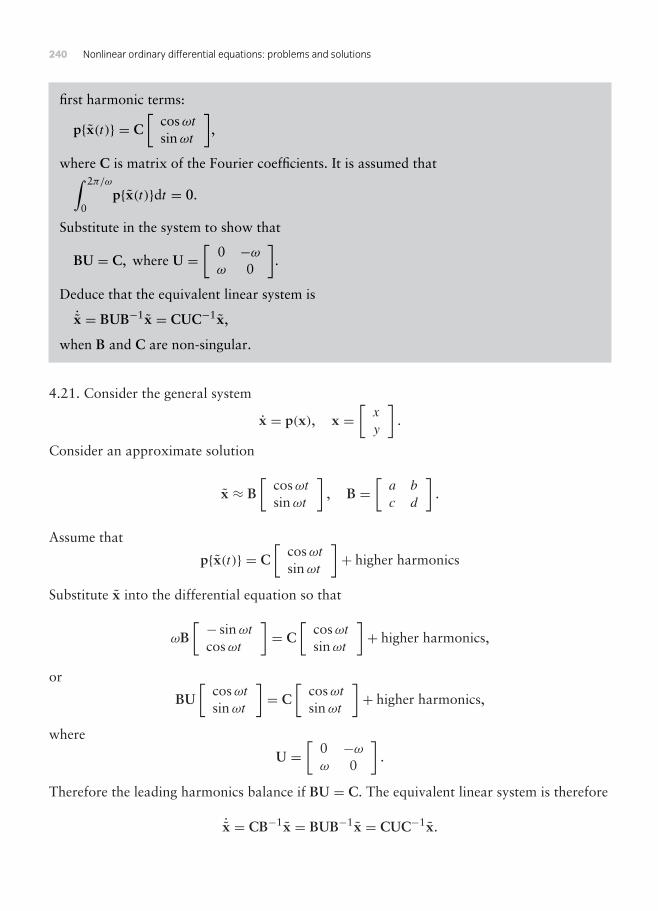
240 Nonlinear ordinary differential equations: problems and solutions
first harmonic terms:
px(t) = C[
cosωtsinωt
],
where C is matrix of the Fourier coefficients. It is assumed that∫ 2π/ω
0px(t)dt = 0.
Substitute in the system to show that
BU = C, where U =[
0 −ωω 0
].
Deduce that the equivalent linear system is
˙x = BUB−1x = CUC−1x,
when B and C are non-singular.
4.21. Consider the general system
x = p(x), x =[x
y
].
Consider an approximate solution
x ≈ B[
cosωtsinωt
], B =
[a b
c d
].
Assume that
px(t) = C[
cosωtsinωt
]+ higher harmonics
Substitute x into the differential equation so that
ωB[ − sinωt
cosωt
]= C
[cosωtsinωt
]+ higher harmonics,
or
BU[
cosωtsinωt
]= C
[cosωtsinωt
]+ higher harmonics,
where
U =[
0 −ωω 0
].
Therefore the leading harmonics balance if BU = C. The equivalent linear system is therefore
˙x = CB−1x = BUB−1x = CUC−1x.

4 : Periodic solutions; averaging methods 241
• 4.22 Use the method of Problem 4.21 to construct a linear system equivalent to the vander Pol equation
x = y, y = −x − ε(x2 − 1)y.
4.22. For the systemx = y, y = −x − ε(x2 − 1)y,
x =[x
y
], p(x) =
[y
−x − ε(x2 − 1)y
].
It has one equilibrium point, at (0, 0). Let
x = B[
cosωtsinωt
]
in the notation of Problem 4.21. Then,
p(x) =
c cosωt + d sinωt14 (−4a + 4εc − 3εa2c − εb2c − 2εabd) cosωt+1
4 (−4b − 2εabc + 4εd − εa2d − 3εb2d) sinωt++ (higher harmonics)
.
Hence
C = c
14 (−4a + 4εc − 3εa2c
−εb2c − 2εabd)
d14 (−4b − 2εabc + 4εd−εa2d − 3εb2d)
.
From Problem 21, we know that
BU =[a b
c d
] [0 −ωω 0
]=
[bω −aωdω −cω
]= C,
given above. Therefore c = bω and d = −aω. Eliminating c and d in the matrix C, we have
C =[
bω −aω14 (−4a + 4εbω − εbω(a2 + b2)) 1
4 (−4b − 4εaω + εa(a2 + b2))
].
Finally from the second rows in BU = C,
−4aω2 = −4a + 4εbω − εbω(a2 + b2),
−4bω2 = −4b − 4εaω + εa(a2 + b2).

242 Nonlinear ordinary differential equations: problems and solutions
These two equations imply ω = 1 and a2 + b2 = 4. As expected for the van der Pol equationthe frequency of the limit cycle is 1 and its amplitude is 2.
To find the equivalent linear equation go back to the general equation
C = BU =[bω −aωdω −cω
].
Its inverse is given by
C−1 = 1ω(bc − ad)
[c a
d b
].
The equivalent linear equation from Problem 2.21 is
˙x = CUC−1x = ω
ad − bc[ac + bd −(a2 + b2)
c2 + d2 −(ac + bd)]x.
• 4.23 Apply the method of Problem 4.21 to construct a linear system equivalent to[x
y
]=
[ε 1−1 ε
] [x
y
]+
[0
−εx2y
],
and show that the limit cycle has frequency given by ω2 = 1− 5ε2 for ε small.
4.23. Consider the system
[x
y
]=
[ε 1−1 ε
] [x
y
]+
[0
−εx2y
].
Equilibrium occurs where
x = εx + y = 0, y = −x + εy − εx2y = 0.
For ε small (< 1), the system has one equilibrium point, at the origin. As in Problem 4.21, let
x = B[
cosωtsinωt
].
Then
p(x) = C[
cosωtsinωt
],
where
C = εa + c
14 (−4a + 4εc − 3εa2c
−εb2c − 2εabd)
εb + d14 (−4b − 2εabc + 4εd−εa2d − 3εb2d)
.

4 : Periodic solutions; averaging methods 243
The requirement
BU =[a b
c d
] [0 −ωω 0
]=
[bω −aωdω −cω
]= C
implies, from the first row,
bω = εa + c, −aω = εb + d.
Hence c = −εa + bω and d = −aω − εb. Elimination of c and d in C leads to
C = bω
14 [−4a(1+ ε2)+ 4εωb+3ε2ar2 − εωbr2]
−aω14 [−4b(1+ ε2)− 4εωa+3ε2br2 + εωar2]
,
where r2 = a2 + b2. The second rows in BU = C imply
−4aω2 − 4εωb = −4a(1+ ε2)+ 4εωb + 3ε2ar2 − εωbr2,
4εωa − 4bω2 = −4b(1+ ε2)− 4εωa + 3ε2br2 + εωar2.
Elimination between these equations leads to
r2 = a2 + b2 = 8, ω2 = 1− 5ε2,
provided ε < 1/√
5.We can choose a and b to be convenient values, since the system is autonomous. If b = 0,
then
C =[
0 −aω14 [−4a(1+ ε2)+ 3ε2a3] 1
4 [−4εωa + εωa3]]
.
The equivalent linear equation is˙x = CUC−1x.
The inverse of C is given by
C−1 =[ −ε −1−ω 0
]/[2√2(1− 5ε2)].
Hence
CUC−1 =[
ε 1−1+ 4ε2 −ε.
].

244 Nonlinear ordinary differential equations: problems and solutions
The eigenvalues of CUC−1 are given by
∣∣∣∣ ε − λ 1−1+ 4ε2 −ε − λ
∣∣∣∣ = 1− 5ε2 + λ2.
Hence the eigenfrequency is given by ω2 = 1− 5ε2, which agrees with the earlier result.
• 4.24 Apply the method of Problem 4.21 to the predator–prey equation (see Section 2.2)
x = x − xy, y = −y + xy,
in the neighbourhood of the equilibrium point (1, 1), by using the displaced approximations
x = m+ a cosωt + b sinωt , y = n+ c cosωt + d sinωt .
Show that m = n, ω2 = 2m− 1 and a2 + b2 = c2 + d2.
4.24. The predator–prey equations
x = x − xy, y = −y + xy, x, y ≥ 0,
have equilibrium points at (0, 0) (a saddle point) and at (1, 1) (a centre) (see Example 2.3). Theequations may be written
x = p(x).
where
p(x) =[x − xy−y + xy
].
Since the equilibrium point (1, 1) is not at the origin, let
x =[m
n
]+ B
[cosωtsinωt
]where B =
[a b
c d
].
Then
p(x) =[ 1
2 (−ac − bd + 2m− 2mn)12 (ac + bd − 2n+ 2mn)
]
+[a − cm− an b − dm− bn−c + cm+ an −d + dm+ bn
] [cosωtsinωt
]+ higher harmonics.
Since
˙x =[bω −aωdω −cω
] [cosωtsinωt
],

4 : Periodic solutions; averaging methods 245
comparison of leading harmonics in the two previous terms implies
−ac − bd + 2m− 2mn = 0, ac + bd − 2n+ 2mn = 0, (i)
bω = a − cm− an, −aω = b − dm− bn, (ii)
dω = −c + cm+ an, −cω = −d + dm+ bn. (iii)
From (i) it follows thatm = n. Equations (ii) and (iii) contain four homogeneous linear equationsin a, b, c and d. Non-trivial solutions for these amplitudes exist if, and only if,
=
∣∣∣∣∣∣∣∣1−m −ω −m 0ω 1−m 0 −mm 0 −(1−m) −ω0 m ω −(1−m)
∣∣∣∣∣∣∣∣= 0,
Symbolic computation gives the expansion as
= (1− 2m+ ω2)2.
Henceω2 = 2m− 1. (iv)
Squaring and adding (ii) and (iii) leads to
(r2 − s2)(ω2 − 1+ 2m) = 0, (v)
and(r2 − s2)(ω2 − 1+ 2m) = 0, (vi)
where r2 = a2 + b2 and s2 = c2 + d2. Hence (v) or (vi) compared with (iv) both imply r = s.
• 4.25 Show that the approximation solution for the oscillations of the equation x = x2−x3
in the neighbourhood of x = 1 is x = c + a cosωt , where
ω2 = c(15c2 − 15c + 4)2(3c − 1)
, a2 = 2c2(1− c2)
3c − 1.
4.25. The system x = x2 − x3, where x = y, has equilibrium points at (0, 0) (a higher-orderequilibrium point) and at (1, 0) (a centre). Let x ≈ c + a cosωt . Then
x − x2 + x3 = 12 (−a2 + 3a2c − 2c2 + 2c3)
+14 (3a
3 − 8ac + 12ac2 − 4aw2) cosωt + higher harmonics.

246 Nonlinear ordinary differential equations: problems and solutions
Hence the constant term and first harmonic vanish if
−a2 + 3a2c − 2c2 + 2c3 = 0,
a(3a2 − 8c + 12c2 − 4ω2) = 0.
From these equations it follows that (a = 0),
ω2 = 14 (3a
2 − 8c + 12c2), a2 = 2c2(1− c)3c − 1
.
Elimination of a2 implies
ω2 = c(15c2 − 15c + 4)2(3c − 1)
.
• 4.26 Use the method of Section 4.2 to obtain approximate solutions of the equation
x + εx3 + x = 0, |ε| 1.
4.26. The systemx + εx2 + x = 0
has one equilibrium point, at the origin. Assume a solution of the form
x = c + a cosωt .
Then
x + εx2 + x = 12 (2c + a2ω2ε)
+ a(1− ω2) cosωt + higher harmonics
The coefficients of the constant term and the first harmonic vanish if
2c + εω2a2 = 0, a(1− ω2) = 0.
Henceω = 1, c = −1
2ε2a2.
Therefore, near the origin the solution by harmonic balance is
x = −12εa
2 + a cos t .
• 4.27 Suppose that the equation x + f (x)x + g(x) = 0 has a periodic solution with phasepath C. Represent the equation in the (x, y) phase plane given by
x = y − F(x), y = −g(x), where F(x) =∫ x
0f (u)du

4 : Periodic solutions; averaging methods 247
(this particular phase plane is known as the Liénard plane.) Let
v(x, y) = 12y2 +
∫ x
0g(u)du,
and by considering dv/dt on the closed path C show that∫CF(x)dy = 0.
On the assumption that van der Pol’s equation x + ε(x2 − 1)x + x = 0 has a periodicsolution approximately of the form x = A cos t , deduce that and ω ≈ 1, A ≈ 2.
4.27. Consider the equationx + f (x)x + g(x) = 0.
In the (x, y) phase plane, lety = x + F(x), y = −g(x),
where
F(x) =∫ x
0f (u)du.
Let
v(x, y) = 12y2 +
∫ x
0g(u)du.
Then
dvdt= d
dt
[12 (x + F(x))2 +
∫ x
0g(u)du
]
= (x + F(x))(x + f (x)x)+ g(x)x= (x + F(x))(−g(x))+ g(x)x
= −F(x)g(x) = F(x)dydt
.
Therefore ∫CF(x)dy =
∫C
dv = 0. (i)
For van der Pol’s equation,x + ε(x2 − 1)x + x = 0,
the (x, y) phase plane is defined by
x = y − ε∫ x
0(u2 − 1)du = yε(1
3x3 − x), y = −x.

248 Nonlinear ordinary differential equations: problems and solutions
Equation (i) above applied to this equation with x = A cosωt becomes
∫ 2π/ω
0F(x)
dydt
dt = −ε∫ 2π/ω
0(1
3A3 cos3 ωt − A cosωt)A cosωtdt
= A2πε
4ω(A2 − 4) = 0.
We conclude that the amplitude of the limit cycle is A = 2.To obtain the frequency, observe that the period T can be expressed as
T =∫ T
0dt = −
∫ 2π/ω
0
1x
dydt
dt (ii)
Now, with x = 2 cosωt ,
y = x + F(x) = −2ω sinωt + ε(
83
cos3 ωt − 2 cosωt)≈ −2ω sinωt ,
for small ε. Hence (ii) becomes
T ≈∫ 2π/ω
0
2ω2 cosωt2 cosωt
dt =∫ 2π/ω
0ω2dt = 2πω.
Since T = 2π/ω, it follows that ω = 1. The limit cycle is therefore given approximately byx = 2 cos t .
• 4.28 Apply the slowly varying amplitude method of Section 4.3 to
x − ε sin x + x = 0, (0 < ε 1),
and show that the amplitude a satisfies a = εJ1(a) approximately. [Use the formula
J1(a) = 1π
∫ π
0sin(a sin u) sin udu
for the Bessel function J1(a): see Abramowitz and Stegun (1965, p. 360).]Find also the approximate differential equation for θ . Using a graph of J1(a) decide how
many limit cycles the system has. Which are stable?
4.28. The slowly varying amplitude method is applied to
x − ε sin x + x = 0, (0 < ε 1).

4 : Periodic solutions; averaging methods 249
10 20 30 40 50a
J1(a)
–0.2
0.2
0.4
0.6
Figure 4.4 Problem 4.28: Bessel function J1(a) plotted against the amplitude a.
The system has one equilibrium point at the origin which is an unstable spiral. In this problemh(x, y) = sin y. Equation (4.28) (in NODE) becomes
a = −εp0(a) = − ε
2π
∫ 2π
0sin(−a sin u) sin udu
= ε
2π
∫ 2π
0sin(a sin u) sin udu
= εJ1(a),
where J1(a) is a Bessel function of order 1. Hence any limit cycles have amplitudes whichare the zeros of the Bessel function J1(a). The graph of J1(a) versus a displaying its oscillatorycharacter is shown in Figure 4.4. This system has an infinite number of limit cycles. After a = 0,the first, third, fifth, etc. zeros correspond to stable limit cycles.
The approximate differential equation for θ is (4.29), namely
θ = −1− ε
ar0(a)
= −1− ε
2πa
∫ 2π
0sin(−a sin u) cos udu
= −1+ ε
2πa
∫ 2π
0sin(a sin u) cos udu
= −1+ ε
2πa
[−cos(a sin u)
a
]2π
0
= −1
Integrating, θ = −t + θ0.

This page intentionally left blank

5 Perturbation methods
Trigonometric identities
The following identities are useful in the application of perturbation methods.
(A) cos3 t = 34 cos t + 1
4cos3t ; sin3 t = 34 sin t − 1
4 sin 3t .
(B) (a cos t + b sin t)3 = 34b(a
2 + b2)+ 14a(a
2 + b2) sin t − 14b(3a
2 − b2) cos 3t
+14a(3b
2 − 1) sin 3t .
(C) (c + a cos t + b sin t)3 = 12c(3a
2 + 3b2 + 2c2)+ 34b(a
2 + b2 + 4c2) cos t
+34a(a
2 + b2 + 4c2) sin t + 32c(b
2 − a2) cos 2t
+3abc sin 2t + 14b(b
2 − 3a2) cos 3t
+14a(3b
2 − a2) sin 3t .
• 5.1 Find all the periodic solutions of x +2x = cos t for all values of 2.
5.1. The general solutions ofx +2x = cos t
arex = A cost + B sint +
2 − 1cos t , (2 = 1),
x = A cost + B sint + 12t sin t , (2 = 1).
• 2 = 1. There are no periodic solutions.• = p, p(= ±1) an integer. General solution is
x = a cospt + b sinpt +
p2 − 1cos t ,
which has period 2π .• = 1/q, q = ±1 an integer. The general solution is
x = a cos(t/q)+ b sin(t/q)+ q2
1− q2 cos t ,
which has period 2πq.

252 Nonlinear ordinary differential equations: problems and solutions
• = p/q, p, q integers, p/q = 1. The general solution is
x = a cos(pt/q)+ b sin(pt/q)+ q2
p2 − q2 cos t ,
which has period 2πq.• = irrational number. The equation has a only one periodic solution
x =
2 − 1cos t ,
and this has period 2π .
• 5.2 Find the first harmonics of the solutions of period 2π of the following:
(i) x − 0.5x3 + 0.25x = cos t ;
(ii) x − 0.1x3 + 0.6x = cos t ;
(iii) x − 0.1x2 + 0.5x = cos t .
5.2. These problems are of the form
x + εh(x, x)+2x = cos t .
In the direct method (see NODE, Section 5.2) we let
x(t) = x0(t)+ εx1(t)+ ε2x2(t)+ · · · .
Direct substitution gives the equations
x0 +2x0 = cos t ,
x1 +2x1 = −h(x0, x0),
and so on.
(i) x − 0.5x3 + 0.25x = cos t . In this problem, h(x, x) = −x3, = 1, = 12 and ε = 0.5.
Therefore x0 satisfies
x0 + 0.25x0 = cos t .
Therefore
x0 = A0 cos 0.5t + B0 sin 0.5t − 43 cos t .

5 : Perturbation methods 253
The constants A0 and B0 must be put equal to zero since otherwise x1 will include non-periodicterms. The second term satisfies
x1 + 0.25x1 = 12
(43
)3
cos3 t = 827(3 cos t + cos 3t).
The general solution is
x1 = A1 cos 0.5t + B1 sin 0.5t − 3227
cos t − 32945
cos 3t .
For the same reason A1 = B1 = 0 to avoid non-periodic terms. Finally
x = −43
cos t + 0.5[−32
27cos t − 32
945cos 3t
]+O(ε2)
= −5227
cos t − 16945
cos 3t +O(ε2).
(ii) x − 0.1x3 + 0.6x = cos t . In this problem, h(x, x) = −x3, = 1, 2 = 3/5 and ε = 1/10.Then x0 satisfies
x0 + 35x0 = cos t .
As in (i), complementary functions must be put equal to zero at each stage to eliminate non-periodic terms. The first term in the expansion of the forced solution is
x0 = −52 cos t .
The second term satisfies
x1 + 35x1 = 1
10
(52
)3
cos3 t = 7564
cos t + 2564
cos 3t .
The particular solution is
x1 = −375128
cos t − 1252688
cos 3t .

254 Nonlinear ordinary differential equations: problems and solutions
The expansion is
x = −52
cos t + 110
[−375
128cos t − 125
2688cos 3t
]+O(ε2)+O(ε2)
= −765256
cos t − 255376
cos 3t +O(ε2)
≈ −2.99 cos t − 0.005 cos 3t
(iii) x − 0.1x2 + 0.5x = cos t . In this case, h(x, x) = −x3, = 1, 2 = 12 and ε = 1/10. Then
x0 satisfies
x0 + 12x0 = cos t .
As in (i), complementary functions must be put equal to zero at each stage to eliminate non-periodic terms. The leading term is therefore
x0 = −2 cos t .
The second term satisfies
x1 + 12x1 = 1
1022 sin2 t = 15 (1− cos 2t).
Hencex1 = 2
5 + 235 cos 2t .
The expansion is
x = −2 cos t + 110
[25+ 2
35cos 2t
]+O(ε2)
= 125− 2 cos t + 2
35cos t + 1
175cos 2t +O(ε2)
• 5.3 Find a first approximation to the limit cycle for Rayleigh’s equation
x + ε(
13 x
3 − x)+ x = 0, |ε| 1,
using the method of NODE, Section 5.9 (Lindstedt’s method).
5.3. In Rayleigh’s equation
x + ε(
13 x
3 − x)+ x = 0, |ε| 1,

5 : Perturbation methods 255
apply the change of scale τ = ωt , so that x satisfies
ω2x′′ − ε(1− 1
3ω2x′2
)ωx′ + x = 0,
where x′ = dx/dτ . Look for periodic solutions which are perturbations of those having period2π . Let
ω = 1+ εω1 + · · · ,
x(ε, τ) = x0(τ )+ εx1(τ )+ · · · .
Substituting these expansions into the differential equation, we have
(1+ 2ωε + · · · )(x′′0 + εx′′1 + · · · )− ε(1− 1
3x′20 + · · ·
)(x′0 + · · · )+ x0 + εx1 + · · · = 0.
Equating coefficients of like powers of ε,
x′′0 + x0 = 0, (i)
x′′1 + x1 = −2ω1x′0 +
(1− 1
3x′20
)x′0. (ii)
Without loss of generality, we may assume the boundary conditions x(0) = a0, x(0) = 0.Applying the expansions to the boundary conditions, we have
x0(0) = a0; x1(0) = 0; . . . , (iii)
x0(0) = 0; x1(0) = 0; . . . , (iv)
and so on. The solution of (i) and (iii) is
x0 = a0 cos τ .
Equation (iv) for x1 becomes
x′′1 + x1 = 2ω1a0 cos τ +(−a0 sin τ + 1
3a30 sin3 τ
)= 2ω1a0 cos τ + a0
(14a
20 − 1
)sin τ − 1
12a30 sin 3τ .
The coefficients of cos τ and sin τ must be zero to avoid secular (non-periodic) terms for x1.Therefore ω1 = 0 and a0 = 2. The leading term in the expansion is
x ≈ 2 cos t .

256 Nonlinear ordinary differential equations: problems and solutions
• 5.4 Use the method of Section 5.9 to order ε to obtain solutions of period 2π , and theamplitude–frequency relation, for
(i) x − εxx + x = 0;
(ii) (1+ εx)x + x = 0.
5.4. (i) In the equationx − εxx + x = 0,
apply the change of scale τ = ωt , so that
ω2x′′ − εωxx′ + x = 0.
Letω = 1+ εω1 + ε2ω2 + · · · ,
x(ε, τ) = x0(τ )+ εx1(τ )+ ε2x2(τ )+ · · · .
Substituting these expansions into the differential equation, it follows that
(1+ εω1 + ε2ω2 + · · · )2(x′′0 + εx′′1 + ε2x′′2 + · · · )− ε(1+ εω1+ ε2ω2 + · · · )(x0+ εx1+ ε2x2 + · · · )(x′0+ εx′1+ ε2x′2 + · · · )+ (x0 + εx1 + ε2x2 + · · · ) = 0.
Equating like powers of ε, we obtain the equations
x′′0 + x0 = 0, (i)
x′′1 + x1 = −2ω1x′′0 + x0x
′0, (ii)
x′′2 + x2 = −(ω21 + 2ω2)x
′′0 − 2ω1x
′′1 + ω1x0x
′0 + x0x
′1 + x′0x1. (iii)
Without loss of generality, we may assume the initial conditions x = a, x = 0 when t = 0,which become x0(0) = a, xi(0) = 0, (i = 1, 2, . . .), x′j (0) = 0, (j = 0, 1, 2, . . .).
Equation (i) has the solution x0 = a cos τ , and (ii) becomes
x′′1 + x1 = 2ω1 cos τ − 12a
2 sin 2τ (iv)
Hence x1 will only have a periodic solution if the coefficient of cos τ is zero. Therefore ω1 = 0.The remaining eqn (iv) has the general solution
x1 = A cos τ + B sin τ + 16a
2 sin 2τ .

5 : Perturbation methods 257
From the initial conditions A = 0 and B = −13a
2. The required second term is
x1 = −13a
2 sin τ + 16a
2 sin 2τ .
Now construct the equation for x2 from (iii), which becomes, on reduction
x′′2 + x2 = 112a(a
2 + 24ω2) cos τ + 13a
3 cos 2τ + 14a
3 cos 3τ .
Hence x2 can only be periodic if ω2 = −a2/24. The frequency–amplitude relation, toorder ε2 is
ω = 1+ ε2ω2 = 1− 124εa
2.
The differential equation for x2 reduces to
x′′2 + x2 = 13a
3 cos 2τ + 14a
3 cos 3τ ,
which has the general solution
x2 = C cos τ +D sin τ − 19 cos 2τ − 1
32 cos 3τ .
From the initial conditions C = 0 and D = 91/288. To order ε2 the expansion for the periodicsolution is
x = a cos τ + ε(−1
3a2 sin τ + 1
6a2 sin 2τ
)+ ε2
(91288 sin τ − 1
9 cos 2τ − 132 cos 2τ
),
where τ = ωt =(1− 1
24ε2a2
)t .
(ii) For the equation
(1+ εx)x + x = 0,
apply the change of scale τ = ωt , so that x satisfies
(1+ εωx′)ω2x′′ + x = 0.
Let
ω = 1+ εω1 + ε2ω2 + · · · ,
x(ε, τ) = x0(τ )+ εx1(τ )+ ε2x2(τ )+ · · · .

258 Nonlinear ordinary differential equations: problems and solutions
Substituting these expansions into the differential equation, it follows that
[1+ ε(1+ εω1 + · · · )(x′0 + εx′1 + · · · )] (1+ εω1 + ε2ω2 + · · · )2× (x′′0 + εx′′1 + ε2x′′2 + · · · )+ (x0 + εx1 + εx2 + · · · ) = 0.
Equating like powers of ε we can obtain the differential equations for x0, x1 and x2, namely,
x′′0 + x0 = 0, (i)
x′′1 + x1 = −2ω1x′′0 − x′0x′′0, (ii)
x′′2 + x2 = −ω21x′′0 − 2ω2x
′′0 − 3ω1x
′0x′′0 − x′′0x′1 − 2ω1x
′′1 − x′0x′′1. (iii)
Assume the initial conditions x = a, x = 0 when t = 0, which become x0(0) = a, xi(0) = 0,(i = 1, 2, . . .), x′j (0) = 0, (j = 0, 1, 2, . . .).
From (i) and the initial conditions, x0 = a cos τ so that x1 satisfies
x′′1 + x1 = −2aω1 cos τ − 12a
2 sin 2τ .
To avoid a growth term in x1 we must put ω1 = 0, leaving the equation
x′′1 + x1 = −12a
2 sin 2τ .
The solution satisfying the initial conditions is
x1 = a2(−1
3 sin τ + 16 sin 2τ
).
The equation for x2 given by (iii) becomes (remember ω1 = 0)
x′′2 + x2 = 16 (12aω2 − a3) cos τ − 1
3a3 cos 2τ + 1
2a3 cos 3τ . (iv)
The secular term in x2 can be eliminated if ω2 = a2/12. We can now find x2 from (iv), whichis, subject to the specified initial conditions,
x2 = a3(
116 cos τ − 2
9 sin τ + 19 sin 2τ − 1
16 cos 3τ).
The perturbation solution is therefore
x = a cos τ + εa2(−1
3 sin τ + 16 sin 2τ
)+ ε2a3
(116 cos τ − 2
9 sin τ + 19 sin 2τ − 1
16 cos 3τ)
where ω = 1+ 112ε
2a3.

5 : Perturbation methods 259
• 5.5 Apply the perturbation method to the equation x +2 sin x = cos t by considering
x +2x + ε2(sin x − x) = cos t ,
with ε = 1, and assuming that is not close to an odd integer, to find perod 2π solutions.Use the Fourier expansion
sin(a cos t) = 2∞∑n=0
(−1)nJ2n+1(a) cos(2n+ 1)t,
where J2n+1 is the Bessel function of order 2n + 1. Confirm that the leading terms aregiven by
x = 12 − 1
[1+2 − 22J11/(2 − 1)] cos t+ 22 − 9
J31/(21) cos 3t .
5.5. Rewrite the equationx +2 sin x = cos t (i)
as a member of the family of equations with parameter ε
x +2x + ε2(sin x − x) = cos t . (ii)
Substitute the perturbation series
x(ε, t) = x0(t)+ εx1(t)+ · · ·
into the differential equation (ii) and equate like powers of ε. Then
x0 +2x0 = cos t , (iii)
x1 +2x1 = −2(sin x0 − x0). (iv)
For not an integer, the only periodic solution (of period 2π ) of (iii) is the forced solution
x0 = 12 − 1
cos t .
Equation (iv) becomes
x1 +2x1 = −2[sin
(cos t2 − 1
)− 12 − 1
cos t]
.
The Fourier series expansion
sin(a cos t) = 2∞∑n=0
(−1)nJ2n+1(a) cos(2n+ 1)t, (v)

260 Nonlinear ordinary differential equations: problems and solutions
where a = 1/(2 − 1), is applied to the right-hand side of (v) so that, to leading order,
x1 +2x1 = − 2
2 − 1
[2(2 − 1)J1
(1
2 − 1
)− 1
]cos t + 2J3
(1
2 − 1
)cos 3t .
The period-2π solution of this equation is
x1 = − 2
(2 − 1)2
[2(2 − 1)J1
(1
2 − 1
)− 1
]cos t + 2
2 − 9J3
(1
2 − 1
)cos 3t .
If we now combine the first two terms and put ε = 1, the result is the perturbation
x = 12 − 1
[1+2 − 22J1
(1
2 − 1
)]cos t + 2
2 − 9J3
(1
2 − 1
)cos 3t .
• 5.6 For the equation x + 2x − 0.1x3 = cos t , where is not near 1, 3, 5, . . . , find, toorder ε, the ratio of the amplitudes of the first two harmonics.
5.6. Consider the family of equations
x +2x − εx3 = cos t ,
and afterwards put ε = 0.1. We are given that is not close to an odd integer, but it may beclose to an even integer. Let
x = x0 + εx1 + · · · .
Substitution into the differential equation leads to
x0 +2x0 = cos t ,
x1 +2x1 = εx30 .
The 2π -periodic solution for x0 is
x0 = 12 − 1
cos t .
The equation for x1 is therefore
x1 +2x1 = 14(2 − 1)
(3 cos t + cos 3t).

5 : Perturbation methods 261
The 2π -periodic solution of this equation is
x1 = 34(2 − 1)2
cos t + 14(2 − 1)(2 − 9)
cos 3t .
to order ε. The approximate solution including the first two harmonics is
x0 + εx1 = 4+ 3ε4(2 − 1)
cos t + ε
4(2 − 1)(2 − 9)cos 3t .
If a3 and a1 are the coefficients of the first two harmonics, then the ratio of the amplitudes is
|a3||a1| =
ε
(4+ 3ε)(2 − 9).
• 5.7 In the equation x+2x+ εf (x) = cos t , is not close to an odd integer, and f (x)is an odd function of x, with expansion
f (a cos t) = −a1(a) cos t − a3(a) cos 3t − · · · .Derive a perturbation solution of period 2π , to order ε.
5.7. In the equation
x +2x + εf (x) = cos t ,
let x = x0 + εx1 + · · · . The two leading terms satisfy
x0 +2x0 = cos t , (i)
x1 +2x1 = −f (x0 + εx1 + · · · ) ≈ −f (x0). (ii)
The 2π -periodic solution of (i) is
x0 =
2 − 1cos t ,
provided is not close to 1 (or any odd integer for higher-order terms).The next term x1 in the perturbation satisfies
x1 +2x1 = −εf(
2 − 1
)= −ε[a1(κ) cos t + a3(κ) cos 3t],

262 Nonlinear ordinary differential equations: problems and solutions
where κ = /(2 − 1). The 2π -periodic solution is
x1 = − a1(κ)
2 − 1cos t − a3(κ)
2 − 9cos 3t .
Hence to order ε,
x = − εa1(κ)
2 − 1cos t − εa3(κ)
2 − 9cos 3t .
• 5.8 The Duffing equation near resonance at =3, with weak excitation, is
x + 9x = ε(γ cos t − βx + x3).
Show that there are solutions of period 2π if the amplitude of the zero-order solution is 0or 2
√(β/3).
5.8. The undamped Duffing equation near resonance at = 3 with weak excitation is
x + 9x = ε(γ cos t − βx + x3).
Let x = x0 + εx1 + · · · . The equations for x0 and x1 are
x0 + 9x0 = 0, (i)
x1 + 9x1 = γ cos t − βx0 + x30 . (ii)
We are searching for 2π -periodic solutions. Equation (i) has the periodic solutionx0 = a0 cos 3t + b0 sin 3t . Substituting x0 into (ii) and expanding, x1 satisfies
x1 + 9x1 = γ cos t − β(a0 cos 3t + b0 sin 3t)+ (a0 cos 3t + b0 sin 3t)3
= γ cos t + 14a0(3a2
0 + 3b20 − 4β) cos 3t+1
4b0(3a20 + 3b2
0 − 4β) sin 3t
+14a0(a
20 − 3b2
0) cos 9t + 14b0(3a2
0 − b20) sin 9t .
The secular terms can be removed by choosing
a0(3a20 + 3b2
0 − 4β) = 0, b0(3a20 + 3b2
0 − 4β) = 0.
Possible solutions are a0 = b0 = 0, or
r0 = √(a20 + b2
0) = 2√(β/3).

5 : Perturbation methods 263
• 5.9 From eqn (5.40), the amplitude equation for the undamped pendulum is
−F = a0
(ω2 − ω2
0 + 18ω
20a
20
).
When ω0 is given, find for what values of ω there are three possible responses. (Find thestationary values of F with respect to a0, with ω fixed. These are the points where theresponse curves of Figure 5.4 (in NODE) turn over.)
5.9. The frequency–amplitude equation is
F = −a0
(ω2 − ω2
0 + 18ω
20a
20
). (i)
We find the stationary points of F with respect to a0 for fixed ω and ω0. Then
dFda0
= ω2 − ω20 + 3
8ω20a
20.
Therefore F is stationary where
a0 = ± 2√
2
ω0√
3
√(ω2
0 − ω2),
if ω2 ≤ ω20. If ω2 > ω2
0, there are no stationary values. There are three possible responses ifω2 < ω2
0.Equation (i) can be expressed in the more convenient form
Q = −a0(a20 − κ),
where Q = 8F/ω20 and κ = 8(ω2
0 − ω2)/ω20. The surface showing the relation between Q and
a0 and κ is shown in Figure 5.1.
a0
Q
k
Figure 5.1 Problem 5.9: Surface showing the frequency–amplitude relation between Q, a0 and κ.

264 Nonlinear ordinary differential equations: problems and solutions
• 5.10 From NODE, eqn (5.42), the amplitude equation for the positively dampedpendulum is
F 2 = r20
k2ω2 +
(ω2 − ω2
0 + 18ω
20r
20
)2
.
By considering d(F 2)/d(r20 ), show that if (ω2−ω2
0)2 ≤ 3k2ω2, then the amplitude equation
has only one real root r0, and three real roots if (ω2 − ω20)
2 > 3k2ω2.
5.10. The amplitude equation for the damped pendulum is
F 2 = r20
k2ω2 +
(ω2 − ω2
0 +18ω2
0r20
)2
.
Let
G = F 2ω20
8ω3k3 , ρ = ω20r
20
8ωk, α = ω2 − ω2
0
kω,
so thatG(ρ) = ρ[1+ (α + ρ)2],
We are only interested in the domain G > 0, ρ > 0.The derivative of G(ρ) is given by
G′(ρ) = 3ρ2 + 4αρ + 1+ α2.
The equation G′(ρ) = 0 has no real solutions if α2 < 3, one real solution if α2 = 3, and tworeal solutions α2 > 3. The cases are discussed below.
• α2 ≤ 3. This is equivalent to
(ω2 − ω20)
2 ≤ 3k2ω2 or ω4 − (2ω20 + 3k2)ω2 + ω4
0 ≤ 0.
The equation
ω4 − (2ω20 + 3k2)ω2 + ω4
0 = 0
has the solutions
ω2 = 12 [(2ω2
0 + 3k2)±√(6ω20 + 9k2)],
both of which give real solutions for ω (we need only consider positive solutions for ω).Hence the system has just one real solution for the amplitude if
12 [(2ω2
0 + 3k2)−√(6ω20 + 9k2)] ≤ ω2 ≤ 1
2 [(2ω20 + 3k2)+√(6ω2
0 + 9k2)].

5 : Perturbation methods 265
• α2 > 3. This is equivalent to
ω4 − (2ω20 + 3k2)ω2 + ω4
0 > 0.
By an argument similar to above the amplitude has three solutions if
ω2 > 12 [(2ω2
0 + 3k2)+√(6ω20 + 9k2)],
or0 < ω2 < 1
2 [(2ω20 − 3k2)+√(6ω2
0 + 9k2)].
• 5.11 Find the equivalent linear form (NODE, Section 4.5) of the expression x+2x−εx3,with respect to the periodic form x = a cos t . Use the linear form to obtain the frequency–amplitude relation for the equation
x +2x − εx3 = cos t .
Solve the equation approximately by assuming that a = a0+ εa1, and show that this agreeswith the first harmonic in NODE, eqn (5.23). (Note that there may be three solutions, butthat this method of solution shows only the one close to /(1−2) cos t .)
5.11. We require the equivalent linear form (see Section 4.5) of the left-hand side of
x +2x − εx3 = cos t .
Assume x ≈ a cos t . Using the identity
cos3 t = 34 cos t + 1
4 cos 3t
and neglecting higher harmonics, we replace −εx3 by
−εa3 cos3 t ≈ −34εa
3 cos t = −34εa
2x.
Therefore the equivalent linear equation is
x +(2 − 3
4εa2)x = cos t .
Hence the 2π -periodic solution is
x =
2 − 1− 34εa
2cos t ,

266 Nonlinear ordinary differential equations: problems and solutions
where the frequency-amplitude equation is
a =
2 − 1− 34εa
2. (i)
Let a = a0 + εa1 + · · · . Then the expansion of eqn (i) gives
a0 + εa1 + · · · =
2 − 1− 34ε(a0 + εa1 + · · · )2
=
2 − 1
[1+ 3
4
εa20
2 − 1
]+O(ε2)
By comparison of the two sides of this equation we deduce
a0 =
2 − 1, a1 = 3
43
(2 − 1)4).
Finally to order ε the first harmonic is
x =
2 − 1cos t + 3
4ε3
(2 − 1)4cos t ,
which agrees with (5.23).
• 5.12 Generalize the method of Problem 5.11 for the same equation by putting x =x(0) + x(1) + · · · , where x(0) and x(1) are the first harmonics to order ε, a cos t and b cos 3t ,say, in the expansion of the solution. Show that the linear form equivalent to x3 is(
34a
2 + 34ab + 3
2b2)x(0) +
(14a
3 + 32a
2b + 34b
3)x(1)/b.
Split the pendulum equation into the two equations
x(0) +2 − ε
(34a
2 + 34ab + 3
2b2)x(0) = cos t ,
x(1) +2 − ε
(14a
3 + 32a
2b + 34b
3)/b
x(1) = 0.
Deduce that a and b must satisfy
a2 − 1− ε
(34a
2 + 34ab + 3
2b2)= ,
b2 − 9− ε
(14a
3 + 32a
2b + 34b
3)= 0.
Assume that a = a0 + εa1 +O(ε2), b = εb1 +O(ε2) and obtain a0, a1 and b1.

5 : Perturbation methods 267
5.12. In the equation
x +2x − εx3 = cos t ,
let x ≈ x(0) + x(1), where x(0) = a cos t and x(1) = b cos 3t and a and b are constants. Then
−εx3 = −ε(a cos t + b cos 3t)3
= −ε[
34a(a
2 + ab + 2b2) cos t + 14 (a
3 + 6a2b + 3b3) cos 3t + (higher harmonics)]
.
Therefore, neglecting higher harmonics,
−εx3 ≈ 34ε(a
2 + ab + 2b2)x(0) + 14ε(a
3 + 6a2b + 3b3)x(1)/b,
and the equivalent linear equations are
x(0) +[2 − 3
4ε(a2 + ab + 2b2)
]x(0) = cos t ,
x(1) +[2 − 1
4ε(a3 + 6a2b + 3b3)
]x(1) = 0.
To ensure that x(0) = a cos t and x(1) = b cos 3t satisfy these equations only if
a[2 − 1− 3
4ε(a2 + ab + 2b2)
]= , (i)
b[2 − 9− 1
4ε(a3 + 6a2b + 3b3)
]= 0. (ii)
Let a = a0 + εa1 + · · · and b = εb1 + · · · . Then (i) and (ii) become
(a0 + εa1 + · · · )[2 − 1− 3
4ε(a0 + · · · )2 + · · · ]= ,
(εb1 + · · · )[(2 − 9)− 1
4ε(a0 + · · · )3 + · · · ]= 0.
Equating like powers of ε, we have
a0 =
2 − 1, a1 = 3
4a3
02−1
= 34
3
(2−1)4,
b1 = 14
a30
2−9= 1
43
(2−1)3(2−1)3.

268 Nonlinear ordinary differential equations: problems and solutions
• 5.13 Apply the Lindstedt method, Section 5.9, to van der Pol’s equation x+ ε(x2−1)x+x = 0, |ε| 1. Show that the frequency of the limit cycle is given by ω = 1− 1
16ε2+O(ε3).
5.13. Linstedt’s method (Section 5.9) is applied to the van der Pol’s equation
x + ε(x2 − 1)x + x = 0, |ε| 1.
Let τ = ωt , so thatω2x′′ + εω(x2 − 1)x′ + x = 0.
We now seek solutions of period 2π . Apply the perturbation expansions x = x0 + εx1 + · · ·and ω = ω0 + εω1 + · · · to this equation:
(ω0 + εω1 + ε2ω2 + · · · )2(x′′0 + εx′′1 + ε2x′′2 + · · · )+ ε(ω0 + εω1 + ε2ω2 + · · · )[(x0 + εx1 + ε2x2 + · · · )2 − 1](x′0 + εx′1 + ε2x2 · · · )+ (x0 + εx1 + ε2x2 + · · · ) = 0
Equating powers of ε, we can obtain the differential equations for the leading terms, namely,
ω20x′′0 + x0 = 0, (i)
ω20x′′1 + x1 = −2ω0ω1x
′′0 − ω0(x
20 − 1)x′0, (ii)
ω20x′′2 + x2 = −2ω0ω1x
′′1 − (2ω0ω2 + ω2
1)x′′0 − (x2
0 − 1)(ω0x′1 + ω1x
′0)− 2ω0x0x
′0x1. (iii)
We search for solutions of period 2π ; since the system is autonomous we can put x′(0) = 0.From (i),
x0 = A0 cos[τ/ω0].We must choose, therefore, ω0 = 1. Substitution of x0 into (ii) leads to
x′′1 + x1 = 2ω1A0 cos τ + (A20 cos2 τ − 1)A0 sin τ
= 2ω1A0 cos τ − (A0 − 14A
30) sin τ + 1
4A30 sin 3τ
Any secular term can be removed by making the coefficients of cos τ and sin τ zero. Thereforewe select A0 = 2 and ω1 = 0. The second term in the expansion is
x1 = A1 cos τ + B1 sin τ − 14 sin 3τ .
Equation (iii) becomes
x′′2 + x2 = 14 (1+ 16ω2) cos t + 2A1 sin t + higher harmonics.

5 : Perturbation methods 269
Hence there are no secular terms if ω2 = − 116 and A1 = 0. Finally the frequency of the limit
cycle is given byω = 1− 1
16ε2 +O(ε3).
• 5.14 Investigate the forced periodic solutions of period 23π for the Duffing equation in
the form x + (1+ εβ)x − εx3 = cos 3t .
5.14. The equationx + (1+ εβ)x − εx3 = cos 3t .
has a forcing term of period 2π/3. Let x = x0 + εx1 + · · · . Then
(x0 + εx1 + · · · )+ (1+ εβ)(x0 + εx1 + · · · )− ε(x0 + εx1 + · · · )3 = cos 3t .
Equating powers of ε, the first two terms satisfy
x0 + x0 = cos 3t , (i)
x1 + x1 = −βx0 + x30 . (ii)
Only the forced part of the solution (i) is of period 2π/3, namely,
x0 = −18 cos 3t .
Equation (ii) becomes
x1 + x1 = 18β cos 3t − 1
833 cos3 3t
= 18β cos 3t − 1
833(
34 cos 3t + cos 9t
)
=
8
(β − 32
4× 82
)cos 3t + higher harmonics
Therefore the leading harmonic in x1 is
x1 = − 82
(β − 32
4× 82
)cos 3t + · · · .
Therefore up to the first harmonic,
x = −8
[1+ ε
8
(β − 32
4× 82
)]cos 3t + · · · .

270 Nonlinear ordinary differential equations: problems and solutions
• 5.15 For the equation x + x + εx3 = 0, |ε| 1, with x(0) = a, x(0) = 0, assume anexpansion of the form x(t) = x0(t) + εx1(t) + · · · , and carry out the perturbation processwithout assuming periodicity of the solution. Show that
x(t) = a cos t + εa3−3
8 t sin t + 132 (cos 3t − cos t)
+O(ε3).
(This expansion is valid, so far as it goes. Why is it not so suitable as those already obtainedfor describing solutions?)
5.15. Apply the expansion x = x0 + εx1 + · · · to the system
x + x + εx3 = 0, x(0) = a, x(0) = 0.
Thus(x0 + εx1 + · · · )+ (x0 + εx1 + · · · )+ ε(x0 + · · · )3 = 0.
Equating to zero the coefficients of like powers of ε, we obtain the equations
x0 + x0 = 0, (i)
x1 + x1 = −x30 , (ii)
subject to the given initial conditions x0 = a cos t . Equation (ii) then becomes
x1 + x1 = −x30 = a3 cos3 t
= 34 cos t + 1
4 cos 3t .
The general solution of this linear second-order equation is
x1 = A1 cos t + B1 sin t + 932 cos t + 3
8 t sin t − 132 cos 3t .
The expansion of the initial conditions implies x1(0) = x1(0) = 0. Therefore A1 and B1 aregiven by
A1 = − 932 + 1
32 = −14 , B1 = 0.
Finally the expansion takes the non-periodic form
x ≈ x0 + x1 = a cos t + εa3[−3
8 t sin t + 132 (cos 3t − cos t)
].
x1 has a term with the factor εt (and we would find that x2 has a term with factor ε2t2,and so on). For any fixed order of approximation the error will increase as t increases, and isunlikely to be small (i.e. the expansion is non-uniform).

5 : Perturbation methods 271
• 5.16 Find the first few harmonics in the solution, period 2π , of x+2x+εx2 = cos t , bythe direct method of Section 5.2. Explain the presence of a constant term in the expansion.
For what values of does the expansion fail? Show how, for small values of , anexpansion valid near = 1 can be obtained.
5.16. Apply the expansion x = x0 + εx1 + ε2x2 + · · · to
x +2x + εx2 = cos t ,
assuming that |ε| 1. Thus
(x0 + εx1 + ε2x2 + · · · )+2(x0 + εx1 + ε2x2 + · · · )+ ε(x0 + εx1 + ε2x2 + · · · )2 = cos t .
The coefficients of the powers ε lead to the perturbation equations
x0 +2x0 = cos t , (i)
x1 +2x1 = −x20 , (ii)
x2 +2x2 = −2x0x1. (iii)
The period 2π solution of (i) is
x0 =
2 − 1cos t .
Equation (ii) then becomes
x1 +2x1 = −
2(2 − 1)−
2(2 − 1)cos 2t .
The period 2π solution of this equation
x1 = −
22(2 − 1)−
2(2 − 1)(2 − 4)cos 2t .
The equation for x2 is
x′′2 +2x2 = −2(
2 − 1cos t
)(−
22(2 − 1)−
2(2 − 1)(2 − 4)cos 2t
)
= 2
22(2 − 1)(2 − 4)[(8−2) cos t +2 cos 3t].

272 Nonlinear ordinary differential equations: problems and solutions
The 2π periodic solution for x2 is
x2 = 2(8−2)
22(2 − 1)2(2 − 4)cos t + 22
22(2 − 1)(2 − 4)(2 − 9)cos 3t .
To order ε2, the 2π periodic solution is
x = − ε
2(2 − 1)+
[
2 − 1+ ε22(8−2)
22(2 − 1)2(2 − 4)
]cos t
− ε
2(2 − 1)(2 − 4)cos 2t + ε222
22(2 − 1)(2 − 4)(2 − 9)cos 3t
The appearance of a constant term indicates that the periodic solution is no symmetricallydisposed about x = 0. The expansion will be unreliable if is close to an integer.
To emphasize that is small, let = εγ , so that the differential equation becomes
x +2x + εx2 = εγ cos t ,
Let = 1+ ε1 + · · · and x = x0 + εx1 + · · · . Then
(x0 + εx1 + · · · )+ (1+ ε1 + · · · )2(x0 + εx1 + · · · )+ ε(x0 + εx1 + · · · )2 = εγ cos t .
Equating powers of ε, we obtainx0 + x0 = 0, (i)
x1 + x1 = −21x0 − εx20 + γ cos t . (ii)
The general solution of (i) isx0 = A0 cos t + B0 sin t .
Substitute this solution into (ii) which becomes
x1 + x1 = −21(A0 cos t + B0 sin t)− ε(A0 cos t + B0 sin t)3 + γ cos t
= −12ε(A
20 + B2
0 )− (21A0 − γ ) cos t − 21B0 sin t + higher harmonics
Secular terms can be removed by putting B0 = 0 and A0 = γ /(21), which is the lead-ing frequency–amplitude relation. Further equations relating amplitude and frequency can beobtained by continuing the perturbation.
• 5.17 Use the method of amplitude-phase perturbation (NODE, Section 5.8) to approxi-mate to the solutions, period 2π , of x + x = ε(γ cos t − xx − βx).

5 : Perturbation methods 273
5.17. In the equationx + x = ε(γ cos t − xx − βx),
let s = t + α and X(ε, s) = x(ε, t) (see Section 5.8). After the change of variable X satisfies
X′′ +X = ε[γ cos(s − α)−XX′ − βX],
where X′ = dX/ds, etc. Let
X(ε, s) = X0(s)+ εX1(s)+ · · · , α = α0 + εα1 + · · · . (i)
We are searching for a 2π -period solution for X(ε, s) and all its coefficients in its perturbationseries. We can also assume, without loss of generality, that X′i (0) = 0 for all i. Substitute theseries
cos(s − α) = cos(s − α0)+ εα1 sin(s − α0)+ · · ·into (i) and equate to zero the coefficients of ε: the result is
X′′0 +X0 = 0, (ii)
X′′1 +X1 = γ cos(s − α0)−X0X′0 − βX0, (iii)
X′′2 +X2 = γα1 sin(s − α0)−X0X′1 −X1X
′0 − βX1. (iv)
From (i), it follows that X0(s) = r0 cos s. Equation (ii) now becomes
X′′1 +X1 = γ cos(s − α0)+ r20 cos s sin s − βr0 cos s
= (cosα0 − βr0) cos s + γ sinα0 sin s + 12r
20 sin 2s.
We need to eliminate the secular terms on the right, so that
cosα0 − βr0 = 0, γ sinα0 = 0.
We can choose α0 = 0 so that r0 = 1/β. For these values X1 satisfies
X′′1 +X1 = 12β2 sin 2s.,
which has the general solution
X1 = a1 cos s + b1 sin s − 16β2 sin 2s.
Using the initial condition, X′1(s) = 0,
X1 = −a1 cos s + 13β2 sin s − 1
6β2 sin 2s.

274 Nonlinear ordinary differential equations: problems and solutions
Equation (iv) now becomes
X′′2 +X2 = 112β3 (1+ 12a1β
4) cos s + 13β(3α1γβ − 1) sin s + higher harmonics.
Non-periodic solutions arise unless
a1 = 112β4 , α1 = 1
3γβ.
Finally
X1 = − 112β4 cos s + 1
3β2 sin s − 16β2 sin 2s.
• 5.18 Investigate the solutions, period 2π , of x+9x+ εx2 = cos t obtained by using thedirect method of NODE, Section 5.2. If x = x0 + εx1 + · · · , show that secular terms firstappear in x2.
5.18. We will use the direct method of Section 5.2 to find, approximately, the 2π periodsolutions of
x + 9x + εx2 = cos t .
Let x = x0 + εx1 + · · · . Then
(x0 + εx1 + · · · )+ 9(x0 + εx1 + · · · )+ ε(x0 + εx1 + · · · )2 = cos t .
Equating like powers of ε, the first few equations are
x0 + 9x0 = cos t , (i)
x1 + 9x1 = −x20 , (ii)
x2 + 9x2 = −2x0x1. (iii)
The period 2π-period solution of (i) is
x0 = a0 cos 3t + b0 sin 3t + 18 cos t .
Now substitute this into the equation for x1:
x1 + 9x1 = −12(a2
0 + b20)+
2
128−
128(16a0 + ) cos 2t
−18a0 cos 4t + 1
2 (−a20 + b2
0) cos 6t − 18b0 sin 2t−1
8b0 sin 4t − a0b0 sin 6t
Secular terms of the form t cos 3t and t sin 3t first appear for x2 through the forcing term−2x0x1.

5 : Perturbation methods 275
• 5.19 For the damped pendulum equation with a forcing term
x + kx + ω20x − 1
6ω20x
3 = F cosωt ,
show that the amplitude–frequency curves have their maxima on ω2 = ω20
(1− 1
8r20
)− 1
2k2.
5.19. The damped pendulum equation with a forcing term is
x + kx + ω20x − 1
6ω20x
3 = F cosωt .
The amplitude–frequency equation for the equation is
r20
[k2ω2 +
(ω2 − ω2
0 + 18ω
20r
20
)2]= F 2, (i)
as given by NODE, (5.42). The family of curves for varying values of F are shown in Figure 5.5(in NODE). At fixed values of r0, there will be two solutions for ω below the maximum andone at the maximum. Equation (i) can be rearranged as a quadratic equation in ω2, namely
r20ω
4 + r20ω
2[k2 − 2ω2
0
(1− 1
8r20
)]+ r2
0ω40
(1− 1
8r20
)2 − F 2 = 0. (ii)
This equation has a repeated solution if
r40
[k2 − 2ω2
0
(1− 1
8r20
)]2 = 4r20
[r20ω
40
(1− 1
8r20
)2 − F 2]
,
or, after rearrangement,
F 2 = 14k
2r20
[2ω2
0
(1− 1
8r20
)− k2
]. (iii)
The repeated solution of (ii), which locates the position of the maximum, is given by
ω2 = ω20
(1− 1
8r20
)− 1
2k2.
Equation (iii) identifies the value of F and the particular path in Figure 5.5 (in NODE) on whichthe maximum occurs.
• 5.20 Show that the first harmonic for the forced van der Pol equation x+ε(x2−1)x+x =F cosωt is the same for both weak and hard excitation, far from resonance.

276 Nonlinear ordinary differential equations: problems and solutions
5.20. In the forced van der Pol equation
x + ε(x2 − 1)x + x = F cosωt ,
let τ = ωt . The equation becomes
ω2x′′ + ωε(x2 − 1)x′ + x = F cos τ , (i)
where x′ = dx/dτ . Hard excitation, far from resonance, is covered in Section 5.10, where it isshown that, in the expansion x = x0 + εx1 + · · · ,
x0 = F
1− ω2 cos τ +O(ε) = F
1− ω2 cosωt +O(ε). (ii)
For soft excitation, let F = εF0, so that (i) becomes
ω2x′′ + ωε(x2 − 1)x + x = εF0 cos τ ,
Let x = x0 + εx1 + · · · for all ε. Then x0 and x1 satisfy the equations
ω2x′′0 + x0 = 0,
ω2x′′1 + ω(x20 − 1)x′0 + x1 = F0 cos τ .
Period 2π solutions are
x0 = 0, x1 = F0
1− ω2 cos τ .
Therefore
x = εx1 +O(ε2) = εF0
1− ω2 cos τ +O(ε2) = F
1− ω2 cosωt +O(ε2),
in which the leading term agrees with (ii).
• 5.21 The orbital equation of a planet about the sun is
d2u
dθ2 + u = k(1+ εu2),
where u = r−1 and r, θ , are polar coordinates, k = γm/h2, γ is the gravitational constant,m is the mass of the planet and h is its moment of momentum, a constant, εku2 is therelativistic correction term, where ε is a small constant.
Obtain a perturbation expansion for the solution with initial conditions u(0) = k(e+ 1),u(0) = 0. (e is the eccentricity of the unperturbed orbit, and these are initial conditions at

5 : Perturbation methods 277
the perihelion: the nearest point to the sun on the unperturbed orbit.) Note that the solutionof the unperturbed equation is not periodic, and that ‘secular’ terms cannot be eliminated.Show that the expansion to order ε predicts that in each orbit the perihelion advancesby 2k2πε.
5.21. The orbital equation of a planet is
u′′ + u = k(1+ εu2),
where u = 1/r and r, θ are polar coordinates, and ε is a small constant. The initial conditionsare
u(0) = k(e + 1), u(0) = 0,
where e is the eccentricity of the unperturbed orbit. Let u = u0 + εu1 + · · · . The leading termssatisfy the differential equations
u′′0 + u0 = k, (i)u′′1 + u1 = ku2
0, (ii)
subject to the initial conditions u0(0) = k(e + 1), u1(0) = 0, u′0(0) = u′1(0) = 0. The generalsolution of (i) is
u0 = A0 cos θ + B0 sin θ + k.From the conditions, A0 = ke, B0 = 0, so that
u0 = k(e cos θ + 1).
Equation (ii) is now
u′′1 + u1 = k3(e cos θ + 1)2 = 12k
3[(2+ e2)+ 4e cos θ + e2 cos 2θ ]. (iii)
Since e is specified, the secular term 2e cos θ cannot be eliminated, which indicates that thesolution will not be periodic. The general solution of this equation is
u1 = A1 cos θ + B1 sin θ + 12k
3(2+ e2)+ ek3θ sin θ − 16e
2k3 cos 2θ .
From the initial conditions A1 = −13k
3(3+ e2), B1 = 0. Hence
u1 = 12k
3(2+ e2)− 13k
3(3+ e2) cos θ + ek3θ sin θ − 16e
2k3 cos 2θ ,
so that
u = k(e cos θ + 1)+ εk3[
12 (2+ e2)− 1
3 (3+ e2) cos θ + eθ sin θ − 16e
2 cos 2θ]+O(ε2).

278 Nonlinear ordinary differential equations: problems and solutions
Let θ = 2π + µ0ε, where |µ| is small. At the next perihelion,
u′(2π + µ0ε) = u′0(2π + µ0ε)+ εu′1(2π + µ0ε)+O(ε2)
= u′0(2π)+ εµ0u′′0(2π)+ εu′1(2π)+O(ε2)
= ε[µ0u′′0(2π)+ u′1(2π)] +O(ε2)
= ε[µ0(−ke)+ 2ek3π)+O(ε2)
The term of order ε vanishes if µ0=2k2π . Hence the perihelion advances by 2k2πε
approximately.
• 5.22 Use the Lindstedt procedure (NODE, Section 5.9) to find the first few terms in theexpansion of the periodic solutions of x + x + εx2 = 0. Explain the presence of a constantterm in the expansion.
5.22. We apply the Lindstedt procedure (Section 5.9) to the equation
x + x + εx2 = 0. (i)
When ε = 0, the frequency of all solutions is 1. Therefore we let the unknown frequency be
ω = 1+ εω1 + · · · , x(ε, t) = x0(t)+ εx1(t)+ · · · .
Apply the change of variable τ = ωt , so that (i) becomes
ω2x′′ + x + εx2 = 0.
We are searching for 2π periodic solutions. Substitution of the perturbations leads to
(1+ εω1 + · · · )2(x′′0 + εx′′1 + · · · )+ (x0 + εx1 + · · · )+ ε(x0 + εx1 + · · · )2 = 0
for all ε. Therefore the leading terms satisfy
x′′0 + x0 = 0, (ii)
x′′1 + x1 = −2ω1x′′0 − x2
0 = 0, (iii)
x′′2 + x2 = −(ω21 + 2ω2)x
′′0 − 2ω1x
′′1 − x2
0 − 2x0x1. (iv)

5 : Perturbation methods 279
Since it is an autonomous system we can simplify the procedure by assuming x(ε, 0) = a andx′(ε, 0) = 0, which implies that x0 = a, x′0(0) = 0, and xi(0) = x′i (0) = 0, (i = 1, 2, . . .). Thesolution of (i) is
x0 = a cos τ ,
so that x1 satisfies
x′′1 + x1 = 2ω1a cos τ − a2 cos2 τ = 2ω1a cos τ − 12a
2(1+ cos 2τ).
To eliminate the secular term put ω1 = 0 (a0 = 0 leads to the solution x = 0). By elementaryintegration follows that
x1 = −12a
2 + 13a
2 cos τ + 16a
2 cos 2τ .
With ω1 = 0, eqn (iv) becomes
x′′2 + x2 = −2ω2x′′0 − x2
0 − 2x0x1
= 2ω2a cos τ − a2 cos2 τ−2a cos τ(−1
2a2 + 1
3a2 cos t + 1
6a2 cos 2t
)
= −16a
2(3+ 2a)+ 16a(5a
2 + 24ω2) cos t − 16a
2(3+ 2a) cos 2t−16a
3 cos 3t
The secular term vanishes if the coefficient of cos t is zero, that is, if ω2 = − 524a
2. Thereforethe frequency–amplitude relation is given by
ω = 1− 524a2ε2 +O(ε3).
Finally
x = x0 + εx1 +O(ε2)
= a cos[(
1− 524ε2
)t
]+ ε
−1
2a2 + 1
3a2 cos
[(1− 5
24ε2
)t
]
+16a2 cos
[2(
1− 524ε2
)t
]+O(ε2).
The constant term indicates that the solution does not have a mean value of zero.

280 Nonlinear ordinary differential equations: problems and solutions
• 5.23 Investigate the forced periodic solutions of period 2π of the equation
x + (4+ εβ)x − εx3 = cos t
where ε is small and β and are not too large. Confirm that there is always a periodicsolution of the form a0 cos 2t + b0 sin 2t + 1
3 cos t , where
a0
(34r
20 + 1
62 − β
)= b0
(34r
20 + 1
62 − β
)= 0.
5.23. In the equation
x + 4x + εβx − εx3 = cos t ,
let x = x0 + εx1 + · · · . Then, equating like powers of ε, we have
x0 + 4x0 = cos t , (i)
x1 + 4x1 = −βx0 + x30 . (ii)
The general solution of (i) is
x0 = a0 cos 2t + b0 sin 2t + 13 cos t .
Substitution of x0 into (ii) implies
x1 + 4x1 = −β(a0 cos 2t + b0 sin 2t + 1
3 cos t)+
(a0 cos 2t + b0 sin 2t + 1
3 cos t)3
= 136(18r2
0 − 12β + 2) cos t + 112 (9r
20 − 12β + 22)(a0 cos 2t + b0 sin 2t)
+ higher harmonics
where r0 = √(a20 + b2
0). The secular terms can be eliminated if
a0
(34r
20 − β + 1
62)= b0
(34r
20 − β + 1
62)= 0.
The solutions are a0 = b0 = 0 or any a0, b0 which satisfy
34r
20 − β + 1
62 = 0.

5 : Perturbation methods 281
• 5.24 Investigate the equilibrium points of x+ ε(αx4− β)x− x+ x3 = 0, (α > β > 0) for0 < ε 1. Use the perturbation method of NODE, Section 5.12 on homoclinic bifurcationto find the approximate value of β/α at which homoclinic paths exist.
5.24. Equilibrium points of
x + ε(αx4 − β)x − x + x3 = 0, x = y, (α > β > 0), (i)
are located at (0, 0), (1, 0) and (−1, 0). Their linear classifications are as follows.
• (0, 0). Near the origin
x − βεx − x = 0.
The solutions of the characteristic equation are
m = 12 [εβ ±
√(ε2β2 + 4)],
which are both real but of opposite signs. Hence (0, 0) is saddle point.• (1, 0). Let x = 1+X. Then the equation becomes
X + ε[α(1+X)4 − β]X − (1+X)+ (1+X)3 = 0.
The linear approximation of the equation is
X + ε(α − β)X + 2X = 0.
The solutions of its characteristic equation are
m = 12 [−ε(α − β)±
√ε2(α − β)2 − 8].
For α > β and ε sufficiently small, (1, 0) is a stable spiral.• (−1, 0). This has the same linearized equation as that for (1, 0). Therefore it is also stable
spiral.
Following the method described in Section 5.12, we let x = x0+ εx1+ · · · and substitute theseries into (i). The differential equations for x0 and x1 are
x0 − x0 + x30 = 0,
x1 + (3x20 − 1)x1 = −(αx4
0 − β)x0.

282 Nonlinear ordinary differential equations: problems and solutions
the zero-order equation. As shown in the same section has the homoclinic solution x0 =√2sech t for x > 0, and x0 = −√2sech t for x < 0. The condition for a homoclinic path
in x > 0 is
∫ ∞
−∞(β − αx4
0(t))x20(t)dt = 0
as in NODE, eqn (5.105). Since x0(t) =√
2sech t , the condition becomes
2β∫ ∞
−∞sech 4
t sinh2tdt − 8α
∫ ∞
−∞sech 8
t sinh2tdt = 0. (ii)
Use the substitution u = tanh t . Then du/dt = sech 2t and the integrals become
∫ ∞
−∞sech 4
t sinh2tdt =
∫ 1
−1u2du = 2
3,
∫ ∞
−∞sech 8
t sinh2tdt =
∫ 1
−1u2(1− u2)du =
∫ 1
−1(u2 − 2u4 + u6)du = 16
105.
Hence condition (ii) becomes
4β3− 128
105α = 0,
so that β/α = 32/35.
• 5.25 Investigate the equilibrium points of x+ ε(αx2−β)x− x+3x5 = 0 , (α,β > 0) for0 < ε 1. Confirm that the equation has an unperturbed time solution x0 = √[sech 2t](see Problem 3.55). Use the perturbation method of Section 5.12 to show that a homoclinicbifurcation takes place for β ≈ 4α/(3π).
5.25. Equilibrium points of
x + ε(αx2 − β)x − x + 3x5 = 0 (i)
are located at (0, 0), (3−1/4, 0) and (−3−1/4, 0). Their linear classifications are as follows.
• (0, 0). Near the origin
x − εβx − x = 0.

5 : Perturbation methods 283
Its characteristic equation has the solutions
m = 12 [εβ ±
√(ε2β2 + 4)].
which are real but of opposite signs. Therefore (0, 0) is a saddle point.• (3−1/4, 0). Let x = 3−1/4 +X. Then the equation becomes
X + ε[α(3−1/4 +X)2 − β]X − (3−1/4 +X)+ 3(3−1/4 +X)5 = 0.
Its linear approximation
X + ε(3−(1/2)α − β)X + 4X = 0,
which implies that (3−1/4, 0) is a spiral for ε sufficiently small.• (−3−1/4, 0). By symmetry (replace x by −x in (i)), this equilibrium point is also a spiral.
If x0 = √(sech 2t), then
x0 = −12sech 3/2
t sinh t ,
x0=−2sech 1/22t + 3sech 5/22t sinh2 2t=sech 1/22t − 3sech 5/22t = x0 − 3x50 .
The condition for a homoclinic path in x > 0 is
∫ ∞
−∞(β − αx4
0(t))x20(t)dt = 0
as in eqn (5.15). Since x0 = √(sech 2t), the condition becomes
β
∫ ∞
−∞sech 32t sinh2 2tdt − α
∫ ∞
−∞sech 42t sinh2 2tdt = 0.
Use the substitutions u = sinh 2t in the first integral and v = tanh t in the second integral, sothat the integrals become
β
2
∫ ∞
−∞u2
(1+ u2)2du− α
∫ 1
−1v2dv = 0,
orβπ
4− α1
3= 0.
Therefore for a homoclinic connection we require β ≈ 4α/3π .

284 Nonlinear ordinary differential equations: problems and solutions
• 5.26 The equation x + εg(x, x)x + f (x) = 0, x = y, 0 < ε 1 is known to have asaddle point at (0, 0) with an associated homoclinic trajectory with solution x = x0(t) forε = 0. Work through the perturbed method of NODE, Section 5.12, and show that anyhomoclinic paths of the perturbed system occur where∫ ∞
−∞g(x0, x0)x
20dt = 0.
If g(x, x) = β − αx2 − γ x20 and f (x) = −x + x3, show that homoclinic bifurcation occurs
approximately where β = (28α + 12γ )/35 for small ε.
5.26. The equationx + εg(x, x)x + f (x) = 0,
is known to have a saddle point at the origin, with an associated homoclinic trajectory withsolution x = x0(t) for ε = 0. As in Section 5.12, let x = x0 + εx1 + · · · . Then the differentialequation becomes
(x0 + εx1 + · · · )+ εg(x0 + εx1 + · · · , x0 + εx1 + · · · )(x0 + εx1 + · · · )
+f (x0 + εx1 + · · · ) = 0.
Hence, expanding g(x0 + εx1 + · · · , x0 + εx1 + · · · ) and f (x0 + εx1 + · · · ), and equating tozero the coefficients of powers of ε, we have
x0 + f (x0) = 0, (i)
x1 + f ′(x0)x1 = −g(x0, x0)x0. (ii)
We are given that x0 satisfies (i) identically. Multiply both sides of (ii) by x0 and confirm that
ddt[x1x0 + x1f (x0)] = −g(x0, x0)x
20 .
Integrate over the infinite interval with respect to t , so that
[x1x0 + x1f (x0)]∞−∞ = −∫ ∞
−∞g(x0, x0)x
20dt .
A necessary condition for x1 and x1 to both approach zero as t →±∞ is that
∫ ∞
−∞g(x0, x0)x
20dt = 0. (iii)

5 : Perturbation methods 285
In the application, g(x, x)=β −αx2− γ x and f (x)= −x+x3. The unperturbed equation is
x− x+ x3=0,
which has the homoclinic solution x0 =√
2sech t in x > 0. The homoclinic path remains forthe perturbed system if (see (iii) above)
I =∫ ∞
−∞(β − αx2
0 − γ x20)x
20dt = 0.
Substitution of x0 leads to
I =∫ ∞
−∞[2βsech 4
t sinh2t − 4αsech 6
t sinh2t − 4γ sech 8 sinh4
t]dt
= 2β23− 4α
415− 4γ
∫ 1
−1(1− u2)u4du (using integrals after (5.106))
= 43β − 16
15α − 4γ
[25− 2
7
]
= 43β − 16
15α − 16
35γ = 0
if β = (28α + 12γ )/35.
• 5.27 Apply Lindstedt’s method to x + εxx + x = 0, 0 < ε 1 where x(0) = a0,x(0) = 0. Show that the frequency–amplitude relation for periodic solutions is given byω = 1− 1
24a20ε
2 +O(ε3).
5.27. Applying Lindtstedt’s (NODE, Section 5.9) method to
x + εxx + x = 0, x(0) = a0, x(0) = 0,
let τ = ωt , ω = 1+ εω1 + ε2ω2 + · · · and x = x0 + εx1 + ε2x2 + · · · . The equation becomes
ω2x′′ + εωxx′ + x = 0,
where x′ = dx/dτ . Substitution of the series into the equation leads to
(1+ εω1 + ε2ω2 + · · · )2(x′′0 + εx′′1 + ε2x′′2 + · · · )+ ε(1+ εω1 + ε2ω2 + · · · )(x0 + εx1 + ε2x2 + · · · )(x′0 + εx′1 + ε2x′2 + · · · )+ (x0 + εx1 + ε2x2 + · · · ) = 0.

286 Nonlinear ordinary differential equations: problems and solutions
Equating to zero the coefficients of the powers of ε, we obtain the differential equations
x′′0 + x0 = 0, (i)
x′′1 + x1 = −2ω1x′′0 − x0x
′0, (ii)
x′′2 + x2 = −(ω1x0 + x1)x′0 − x0x
′1 − (ω2
1 + 2ω2)x′′0 − 2ω1x
′′1. (iii)
The perturbation initial conditions for x(0) = a and x′(0) = 0 become
x0(0) = a0, xi(0) = 0, (i = 1, 2, . . .), x′j (0) = 0, (j = 0, 1, 2, . . .).
The solution of (i) subject to the initial conditions is x0 = a cos τ . Equation (ii) then becomes
x′′1 + x1 = 2ω1a0 cos τ + 12a
20 sin 2τ .
Periodicity for x1 requires ω1 = 0, so that x1 satisfies
x′′1 + x1 = 12a
20 sin 2τ .
The solution subject to x1(0) = x′1(0) = 0 is
x1 = 16a
20(2 sin τ − sin 2τ).
Substitution of x0 and x1 into (iii), the equation for x2, gives
x′′2 + x2 = 112 (a
30 + 24a0ω2) cos τ − 4a3
0 cos 2τ + 3a30 cos 3τ .
Secular terms can be eliminated by choosing ω2 = −a20/24. Therefore the frequency-amplitude
is given by
ω = 1− 124a
20ε
2 +O(ε3).
• 5.28 Find the first three terms in a direct expansion for x in powers of ε for period 2πsolutions of the equation x +2x − εx2 = cos t , where 0 < ε 1 and = an integer.
5.28. In the equation
x +2x − εx2 = cos t ,

5 : Perturbation methods 287
let x = x0 + εx1 + ε2x2 + · · · .Therefore
(x0 + εx1 + ε2x2 + · · · )+2(x0 + εx1 + ε2x2 + · · · )− ε(x0 + εx1 + ε2x2 + · · · )2 = cos t .
Equating like powers of ε leads to the equations
x0 +2x0 = cos t , (i)
x1 +2x1 = x20 , (ii)
x2 +2x2 = 2x0x1. (iii)
The 2π -periodic solution of (i) is
x0 = cos t2 − 1
. (iv)
Equation (ii) becomes
x1 +2x1 = − sin2 t
(2 − 1)2= − 1
2(2 − 1)2(1− cos 2t).
The 2π periodic solution is
x1 = 12(2 − 1)2
(12 +
cos 2t2 − 4
). (v)
Equation (iii) is
x2 +2x2 = − sin t22(2 − 1)3
+ sin t cos 2t2(2 − 1)3(2 − 4)
= 7 − 22
42(2 − 1)3(2 − 4)sin t + 1
4(2 − 1)3(2 − 4)sin 3t
The 2π periodic solution of this equation is
x2 = 7 − 22
42(2 − 1)4(2 − 4)sin t + 1
4(2 − 1)3(2 − 4)(2 − 9)sin 3t . (vi)
The periodic solution can be constructed by substituting x, x1, x2 from (iv), (v) and (vi) into
x = x0 + εx1 + ε2x2 +O(ε3).

This page intentionally left blank

6 Singular perturbationmethods
• 6.1 Work through the details of NODE, Example 6.1 to obtain an approximate solutionof x + x = εx3, with x(ε, 0) = 1, x(ε, 0) = 0, with error O(ε3) uniformly on t ≥ 0.
6.1. Substitute the expansion
x(ε, t) = x0(t)+ εx1(t)+ ε2x2(t)+ · · ·
into the equation
x + x = εx3,
to give
(x0(t)+ εx1(t)+ ε2x2(t)+ · · · )+ (x0(t)+ εx1(t)+ ε2x2(t)+ · · · ) =ε(x0(t)+ εx1(t)+ ε2x2(t)+ · · · )3.
The initial conditions are
x0(0) = 1, x1(0) = 0, x2(0) = 0, . . . ;
x0(0) = 0, x1(0) = 0, x2(0) = 0, . . . .
The terms in the perturbation series satisfy the differential equations
x0 + x0 = 0, (i)
x1 + x1 = x30 , (ii)
x2 + x2 = 3x20x1. (iii)
The solution of (i) which satisfies the initial conditions is x0= cos t . Equation for x1given by (ii)
x1 + x1 = cos3 t = 34 cos t + 1
4 cos 3t .

290 Nonlinear ordinary differential equations: problems and solutions
Hence
x1 = A cos t + B sin t + 38 t sin t − 1
32 cos 3t .
The initial conditions imply A = 132 and B = 0, so that
x1 = 132 cos t + 3
8 t sin t − 132 cos 3t .
In (iii)
3x20x1 = 3
128 (2 cos t − cos 3t − cos 5t + 12t sin t + 12t sin 3t),
so that
x2 + x2 = 3x20x1 = 3
128 (2 cos t − cos 3t − cos 5t + 12t sin t + 12t sin 3t).
The solution satisfying x2(0) = x′2(0) = 0 is
x2= 11024 (23 cos t − 72t2 cos t −24 cos 3t + cos 5t + 96t sin t −36t sin 3t).
Now let
t = τ + εT1(τ )+ ε2T2(τ )+ · · · . (iv)
Substitute for t into the expressions for x0(t), x1(t) and x2(t). They
x0 = cos[τ + εT1(τ )+ ε2T2(τ )] +O(ε3)
= cos τ − εT1(τ ) sin τ + ε2(−1
2T1(τ )2 cos τ − T2(τ ) sin τ
)+O(ε3).
x1 = 132 cos(τ + εT1(τ ))+ 3
8ε(τ + εT1(τ )) sin(τ + εT1(τ ))
− 132 cos 3(τ + εT1(τ )) = 1
32 [cos τ − cos 3τ + 12τ sin τ ]+ 1
32εT1(τ )[11 sin τ + 12τ cos τ + 3 sin 3τ ] +O(ε2).
x2 = 11024 (23 cos τ − 72τ2 cos τ − 24 cos 3τ + cos 5τ + 96τ sin τ
− 36τ sin 3τ)+O(ε).

6 : Singular perturbation methods 291
In the expansion x(ε, t) = x0(t)+ εx1(t)+ ε2x2(t)+ · · · , the zero-order coefficient is cos τ . Thecoefficient of ε is
−T1(τ ) sin τ + 132 (cos τ − cos 3τ + 12τ sin τ).
The growth term can be eliminated by choosing
T1(τ ) = 38τ .
The coefficient of ε2 is
− 12T1(τ )
2 cos τ − T2(τ ) sin τ + 132T1(τ )[11 sin τ + 12τ cos τ + 3 sin 3τ ]
+ 11024 (23 cos τ − 72τ2 cos τ − 24 cos 3τ + cos 5τ + 96τ sin τ − 36τ sin 3τ)
= −T2(τ ) sin τ + 57256τ sin τ + 23
1024 cos τ − 241024 cos 3τ + 1
1024 cos 5τ
after substituting T1(τ ) = 38τ . The secular term can be eliminated by choosing T2(τ ) = 57
256τ .Hence from (iv) the time perturbation is
t = τ + 38ετ + 57
256ε2τ +O(ε3), (v)
and in terms of τ the solution becomes
x = cos τ + 132ε(cos τ − cos 3τ)+ 1
1024ε2(23 cos τ − 24 cos 3τ + cos 5τ)+O(ε3).
The period of this expression in τ is 2π , and the corresponding t-period is obtained from (v).
• 6.2 How does the period obtained by the method of Problem 6.1 compare with thatderived in Problem 1.34?
6.2. The equation in Problem 1.34 is, with a change of notation,
X +X = ε′X3, (i)
and, the period T of this pendulum equation (as in Problem 6.1) in terms of the amplitude awas shown to be
T = 2π(1+ 3
8ε′a2 + 57
256ε′2a4
)+O(a6).

292 Nonlinear ordinary differential equations: problems and solutions
In Problem 6.1 the initial condition given is x(0) = 1. This can be changed to a by thesubstitution of x = X/a into the differential equation in Problem 6.1, so that
X +X = ε
a2X3
andX(0, ε) = a. This is equivalent to (i) if ε′ is replaced by ε/a2. From Problem 6.1, the relationbetween t and τ is
t = τ + 38ετ + 57
256ε2τ +O(ε3),
and the solution is 2π periodic in τ . Hence the period T ′, say, is given by,
T ′ = 2π[1+ 3
8ε + 57256ε
2 +O(ε3)]
= 2π[1+ 3
8aε′ + 57
256a2ε′2 +O(ε′3)
]≈ T .
for aε′ small enough.
• 6.3 Apply the method of Problem 6.1 to the equation x+x = εx3+ε2αx5 with x(ε, 0) = 1,x(ε, 0) = 0. Obtain the period to order ε3, and confirm that the period is correct for thependulum when the right-hand side is the first two terms in the expansion of x − sin x.(Compare the result of Problem 1.33. To obtain the required equations simply add theappropriate term to the right-hand side of the equation for x2 in Example 6.1 in NODE.)
6.3 The equation
x + x = εx3 + ε2αx5,
is as in Problem 6.1, but with the additional term ε2αx5 which is of order ε2. As in Problem 6.1,we substitute the expansion
x(ε, t) = x0(t)+ εx1(t)+ ε2x2(t)+ · · · ,
into the equation and apply the initial conditions
x0(0) = 1, x1(0) = 0, x2(0) = 0, . . . ;
x0(0) = 0, x1(0) = 0, x2(0) = 0, . . . .

6 : Singular perturbation methods 293
The order zero and order ε terms will be the same so that, with
t = τ + εT1(τ )+ ε2T2(τ )+ · · · ,
we also find that x0 = cos τ , T1(τ ) = 38τ and
x1 = 132 (cos τ − cos 3τ).
The term ε2αx5 will first appear in the equation for x2, which will now become
x2 + x2 = 3x20x1 + αx5
0
= 1128 [(6+ 8α) cos t + (−3+ 40α) cos 3t + (−3+ 8α) cos 5t
+ 36t sin t + 36t sin 3t]
using the expansion
cos5 t = 116 (10 cos t + 5 cos 3t + cos 5t),
The solution of the differential equation satisfying the given initial conditions is
x2 = 13072 [(69+ 128α − 216t2) cos t − (72+ 120α) cos 3t
+ (3− 8α) cos 5t + (288+ 960α)t sin t − 108t sin 3t].
Putting t = τ + · · · in (i), and using eqn (iv) from Problem 6.1, the coefficient of ε2 becomes
− T2(τ ) sin τ + 13072 [(69+ 128α) cos τ − (72+ 120α) cos 3τ
+ (3− 8α) cos 5τ + (684+ 960α)τ sin τ ]
The secular term can be eliminated by choosing
T2(τ ) = 57 + 80α256
τ .
We can compare the result with that obtained from the pendulum equation in Problem 1.33.The exact pendulum equation is
x + sin x = 0,

294 Nonlinear ordinary differential equations: problems and solutions
which can be approximated by
x + x − 16x
3 + 1120x
5 = 0.
This is the same equation as the one in this problem if ε = 16 and ε2α = − 1
120 , so that α = − 310 .
Therefore the timescale becomes
t = τ + εT1(τ )+ ε2T2(τ )+ · · ·
=[1+ 3
8ε + 57+80α256 ε2
]τ +O(ε3)
=[1+ 1
16 + 113072
]τ +O(ε3).
The period obtained using this timescale agrees with that of Problem 1.33.
• 6.4 Use the substitution to show that the case considered in Problem 6.1 (the equation isx + x = εx3) covers all boundary conditions x(ε, 0) = a, x(ε, 0) = 0.
6.4. The equation in Problem 6.1 is
x + x = εx3.
Apply the transformation x(ε, t) = X(ε, t)/a. Then the equation becomes
X +X = εX3/a2,
with the initial conditions X(ε, 0) = a, X(ε, 0) = 0. Finally replace ε/a2 by ε′ so that X satisfies
X +X = ε′X3.
This assumes that ε′ remains small. Hence solutions for general initial conditions subject to theprevious restriction are included in Problem 6.1.
• 6.5 The equation for the relativistic perturbation of a planetary orbit is
d2u
dθ2 + u = k(1+ εu2)
(see Problem 5.21). Apply the coordinate perturbation technique to eliminate the secularterm in u1(θ) in the expansion u(ε, θ) = u0(θ)+ εu1(θ)+ · · · , with θ = φ + εT1(φ)+ · · · .

6 : Singular perturbation methods 295
Assume the initial conditions u(0) = k(1 + e), du(0)/dθ = 0. Confirm that the perihelionof the orbit advances by approximately 2πεk2 in each planetary year.
6.5. The relativistic equation is
d2u
dθ2 + u = k(1+ εu2),
subject to the initial conditions u(ε, 0) = k(1 + e) and x′(ε, 0) = 0. Let u(ε, θ) = u0(θ) +εu1(θ)+ · · · , and substitute this series into the differential equation:
d2
dθ2 (u0 + εu1 + · · · )+ (u0 + εu1 + · · · ) = k[1+ ε(u0 + εu1 + · · · )2].
Equating like powers of ε, we have
d2u0
dθ2 + u0 = k, (i)
d2u1
dθ2 + u1 = ku20. (ii)
The initial conditions become
u0(0) = k(1+ e), ui(0) = 0, (i = 1, 2, . . . ), u′j (0) = 0, (j = 0, 1, 2, . . . ).
Therefore, from (i),
u0 = k(1+ e cos θ).
Equation (ii) becomes
d2u1
dθ2 + u1 = k3(1+ e cos θ)2 = k3[12 (2+ e2)+ 2e cos θ + 12e
2 cos 2θ].
The general solution is
u1(θ) = A cos θ + B sin θ + 12k
3(2+ e2)+ k3eθ sin θ − 16e
2k3 cos 2θ .
The initial conditions u1(0) = u′1(0) = 0 imply
A+ 12k
3(e2 + 2)− 16k
3e2 = 0, B = 0.

296 Nonlinear ordinary differential equations: problems and solutions
Therefore A = −13k
3(e2 + 3), and the required solution is
u1(θ) = 12k
3(2+ e2)− 13k
3(e2 + 3) cos θ + k3eθ sin θ − 16e
2k3 cos 2θ .
Finally
u(ε, θ) = u0(θ)+ εu1(θ) · · ·= +k(1+ e cos θ)+ εk3[12 (2+ e2)− 1
3 (e2 + 3) cos θ
+eθ sin θ − 16e
2 cos 2θ ] +O(ε2)
Now introduce the expansion for the angle θ :
θ = φ + εT1(φ)+ · · · .
where φ is the strained coordinate. Then
u(ε,φ + εT1(φ)+ · · · ) = u0(φ + εT1(φ)+ · · · )+ εu1(φ + εT1(φ)+ · · ·)+ · · ·= k(1+ e cosφ − eεT1(φ) sinφ)+ εk3[12 (2+ e2)− 1
3 (e2 + 3) cosφ
+ eφ sinφ−16e
2 cos 2φ] +O(ε2)
The non-periodic φ sinφ term can be eliminated by choosing T1(φ) = k2φ. The period in θ isgiven by
2πθ = 2π(1+ εk2 + · · ·).
Hence the correction, which is the advance of the perihelion, is approximately 2πεk2.
• 6.6 Apply the multiple-scale method to van der Pol’s equation x + ε(x2 − 1)x + x = 0.Show that, if x(0) = a and x(0) = 0, then for t = O(ε−1),
x = 21+ [(4/a2)− 1]e−εt −(1/2) cos t .
6.6. The van der Pol equation is
x + ε(x2 − 1)x + x = 0. (i)
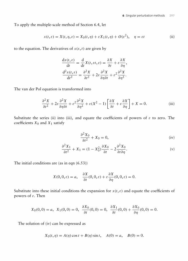
6 : Singular perturbation methods 297
To apply the multiple-scale method of Section 6.4, let
x(t , ε) = X(t , η, ε) = X0(t , η)+ εX1(t , η)+O(ε2), η = εt (ii)
to the equation. The derivatives of x(ε, t) are given by
dx(t , ε)dt
= ddtX(t , εt , ε) = ∂X
∂t+ ε ∂X
∂η,
d2x(t , ε)dt2
= ∂2X
∂t2+ 2ε
∂2X
∂η∂t+ ε2 ∂
2X
∂η2 .
The van der Pol equation is transformed into
∂2X
∂t2+ 2ε
∂2X
∂η∂t+ ε2 ∂
2X
∂η2 + ε(X2 − 1)[∂X
∂t+ ε ∂X
∂η
]+X = 0. (iii)
Substitute the series (ii) into (iii), and equate the coefficients of powers of ε to zero. Thecoefficients X0 and X1 satisfy
∂2X0
∂t2+X0 = 0, (iv)
∂2X1
∂t2+X1 = (1−X2
0)∂X0
∂t− 2
∂2X0
∂t∂η. (v)
The initial conditions are (as in eqn (6.53))
X(0, 0, ε) = a,∂X
∂t(0, 0, ε)+ ε ∂X
∂η(0, 0, ε) = 0.
Substitute into these initial conditions the expansion for x(t , ε) and equate the coefficients ofpowers of ε. Then
X0(0, 0) = a, X1(0, 0) = 0,∂X0
∂t(0, 0) = 0,
∂X1
∂t(0, 0)+ ∂X0
∂η(0, 0) = 0.
The solution of (iv) can be expressed as
X0(t , η) = A(η) cos t + B(η) sin t , A(0) = a, B(0) = 0.

298 Nonlinear ordinary differential equations: problems and solutions
Equation (v) becomes
∂2X1
∂t2+X1 = [1− (A(η) cos t + B(η) sin t)2](−A(η) sin t + B(η) cos t)
− 2(−A′(η) sin t + B ′(η) cos t)
= 14 [4B(η)− A(η)2B(η)− B(η)3 − 8B ′(η)] cos t
+ 14 [−4A(η)+ A(η)3 + A(η)B(η)2 + 8A′(η)] sin t
+ 14B(η)[B(η)2 − 3A(η)2] cos 3t + 1
4A(η)[A(η)2 − 3B(η)2] sin 3t
To avoid secular growth the coefficients of cos t and sin t are equated to zero so that B and Asatisfy the differential equations
4B(η)− A(η)2B(η)− B(η)3 − 8B ′(η) = 0,
−4A(η)+ A(η)3 + A(η)B(η)2 + 8A′(η) = 0.
The initial condition B(0) = 0 in (vi) implies B(η) = 0 for all η, so that A(η) satisfies
8A′(η) = A(η)(4− A(η)2).
This is a separable equation with solution given by
8∫
dAA(4− A2)
=∫
dη + C = η + C,
so that
A2
|A2 − 4| = eCeη,
where C is a constant. By (vi), A(0) = a, leading to
A2 = 4KK − e−η
= 4a2
a2 + (4− a2)e−η= 4a2
a2 + (4− a2)e−εt.
Finally, form (vi), to the first order
x = X0 = A(η) cos t = 2a[a2 + (4− a2)e−εt ]1/2 cos t .
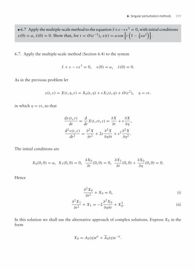
6 : Singular perturbation methods 299
• 6.7 Apply the multiple-scale method to the equation x+x−εx3 = 0, with initial conditions
x(0) = a, x(0) = 0. Show that, for t = O(ε−1), x(t) = a cost(1− 3
8εa2)
.
6.7. Apply the multiple-scale method (Section 6.4) to the system
x + x − εx3 = 0, x(0) = a, x(0) = 0.
As in the previous problem let
x(t , ε) = X(t , η, ε) = X0(t , η)+ εX1(t , η)+O(ε2), η = εt .
in which η = εt , so that
dx(t , ε)dt
= ddtX(t , εt , ε) = ∂X
∂t+ ε ∂X
∂η,
d2x(t , ε)dt2
= ∂2X
∂t2+ 2ε
∂2X
∂η∂t+ ε2 ∂
2X
∂η2 .
The initial conditions are
X0(0, 0) = a, X1(0, 0) = 0,∂X0
∂t(0, 0) = 0,
∂X1
∂t(0, 0)+ ∂X0
∂η(0, 0) = 0.
Hence
∂2X0
∂t2+X0 = 0, (i)
∂2X1
∂t2+X1 = −2
∂2X0
∂η∂t+X3
0. (ii)
In this solution we shall use the alternative approach of complex solutions. Express X0 in theform
X0 = A0(η)eit + A0(η)e−it .

300 Nonlinear ordinary differential equations: problems and solutions
Equation (ii) becomes
∂2X1
∂t2+X1 = −2iA′0(η)+ 2iA
′0(η)+ [A0(η)eit + A0(η)e−it ]3
= −2iA′0(η)eit + 2iA
′0(η)e
−it + A30(η)e
3it + 3A20(η)A0(η)eit
+ 3A0(η)A20(η)e
−it + A30(η)e
−3it
= [−2iA′0(η)+ 3A20(η)A0(η)]eit + [2iA
′0(η)+ 3A0(η)A
20(η)]e−it
+ (higher harmonics)
Secular terms can be removed if
−2iA′0(η)+ 3A20(η)A0(η) = 0. (iii)
Let A0(η) = ρ(η)eiα(η). Then (iii) becomes
−2i(ρ′eiα + iρα′eiα)+ 3ρ3eiα = 0, or (2ρα′ + 3ρ3)− 2iρ′ = 0.
The real and imaginary parts of this equation are zero if
ρ′(η) = 0, 2α′(η)+ 3ρ(η)2 = 0.
Therefore ρ(η) = k, and α′(η) = −32k
2, which implies α(η) = −32k
2η +m. Therefore
X0(t , η) = kei(m−(3/2)k2η+t) + ke−i(m−(3/2)k2η+t) = 2k cos(m− 32k
2η + t).
The initial conditions imply a = 2k cosm and 2k sinm = 0, so that m = 0 and k = 12a. Finally
x ≈ a cos[(1− 38εa
2)t]
as required.
• 6.8 Obtain the exact solution of the equation in Example 6.9 namely,
εd2y
dx2 + 2dydx+ y = 0, y(0) = 0, y(1) = 1,
and show that it has the first approximation equal to that obtained by the matching method.

6 : Singular perturbation methods 301
6.8. Example 6.9 concerns the approximate solution of the boundary-value problem
εd2y
dx2 + 2dydx+ y = 0, y(0) = 0, y(1) = 1, 0 < x < 1.
This a second-order linear differential equation having the characteristic equation
ελ2 + 2λ+ 1 = 0.
The solutions of this equation are
λ1, λ2 = 12ε[−2±√(4− 4ε)] = 1
ε[−1±√(1− ε)].
Subject to the boundary conditions the solution is
y(x, ε) = eλ1x − eλ2x
eλ1 − eλ2.
For small ε,
λ1 = 1ε[−1+√(1− ε)] = 1
ε[−1+ 1− 1
2ε +O(ε2)] = −12 +O(ε).
Hence, approximately,
y(x, ε) ≈ e−(1/2)x − e−2x/ε
e−(1/2) − e−2/ε . (i)
Since x = O(1) but not o(1), that is, x is not ‘small’, the terms e−2x/ε and e−2/ε are exponentiallysmall, so that
y(x, ε) ≈ e(1/2)−(1/2)x = yO(ε, x),
the outer solution given by (6.99).In the boundary layer, let x = ξε. Then, from (i),
y(x, ε) ≈ e−(1/2)ξε − e−2ξ
e−(1/2) − e−2/ε
≈ e−(1/2)ξε − e−2ξ
e−(1/2)(neglecting the exponentially small term)
= e1/2[1− e−2ξ ] +O(ε)

302 Nonlinear ordinary differential equations: problems and solutions
Hence
y(x, ε) ≈ e1/2[1− e−2ξ ] = e1/2[1− e−2x/ε] = yI(x, ε),
which agrees with the inner approximation given by (6.113) (in NODE).
• 6.9 Consider the problem
εy′′ + y′ + y = 0, y(ε, 0) = 0, y(ε, 1) = 1,
on 0 ≤ x ≤ 1, where ε is small and positive.
(a) Obtain the outer approximation
y(ε, x) ≈ yO = e1−x , x fixed, ε→ 0+;
and the inner approximation
y(ε, x) ≈ yI = C(1− e−x/ε), x = O(ε), ε→ 0+,
where C is a constant.
(b) Obtain the value of C by matching yO and yI in the intermediate region.
(c) Construct from yO and yI a first approximation to the solution which is uniform on0 ≤ x ≤ 1.
Compute the exact solution, and show graphically yO, yI, the uniform approximationand the exact solution.
6.9. The system is
εy′′ + y′ + y = 0, y(ε, 0) = 0, y(ε, 1) = 1.
(a) Put ε = 0 in the equation so that the outer solution satisfies y′O+ yO = 0 subject to yO = 1at x = 1. Hence
yO = Ae−x = e1−x . (i)
Let x = ξε. Then eqn (i) is transformed into
d2y
dξ2 +dydξ+ εy = 0
For small ε, the inner approximation yI satisfies
d2y
dξ2 +dydξ= 0,

6 : Singular perturbation methods 303
for x = O(ε) and such that yI = 0 at ξ = 0. Hence
yI = C + Be−ξ = C(1− e−ξ ) = C(1− e−x/ε)
for x = O(ε).(b) The constant C in the previous equation can be found by matching the outer and innerapproximations as follows. Let x = η√ε. Then
yO = e1−x = e1−η√ε = e+O(ε), yI = C(1− e−x/ε) = C(1− e−η/√ε)
= C + o(1),
as ε→ 0+. These match to the lowest order if C = e. Therefore the inner approximation is
yI = e(1− e−x/ε). (ii)
(c) Consider
q(x, ε) = yO + yI = e1−x + e(1− e−x/ε).
If x = O(1), then
q(x, ε) = e1−x + e+O(ε) (iii)
as ε→ 0. If x = ξε where ξ = O(1), then
q(ξε, ε) = e1−ξε + e(1− e−ξ ) = e+ e(1− e−ξ )+O(ε). (iv)
Comparison of (i) and (ii) with (iii) and (iv) shows that both contain the unwanted term e.Hence the composite uniform approximation is
yC = yO + yI − e = e(e−x − e−x/ε).
• 6.10 Repeat the procedure of Problem 6.9 for the problem εy′′ + y′ + xy = 0, y(0) = 0,y(1) = 1 on 0 ≤ x ≤ 1.
6.10. Consider the system
εy′′ + y′ + xy = 0, y(0) = 0, y(1) = 1.
The outer approximation satisfies y′ + xy = 0 with y(1) = 1, for y = O(1). Therefore
yO = Ae−(1/2)x2 = e(1/2)(1−x2).

304 Nonlinear ordinary differential equations: problems and solutions
For the inner approximation, let x = ξε, so that
d2y
dξ2 +dydξ+ ε2y = 0.
For ε small, y satisfies, for ξ = O(1),
d2y
dξ2 +dydξ= 0, y(0) = 0.
Therefore
yI = C + Be−ξ = C(1− e−ξ ) = C(1− e−x/ε).
To match the outer and inner approximations, let x = η√ε. Then
yO = e(1/2)(1−η2ε) = e1/2 +O(ε),
and
yI = C(1− e−η/√ε) = C + o(1).
Hence C = e1/2
To obtain uniform approximation, consider
q(x, ε) = yO + yI = e(1/2)(1−x2) + e1/2(1− e−x/ε).
If x = O(1), then
q(x, ε) = e(1/2)(1−x2) + e1/2 +O(ε). (i)
Let x = ξε where ξ = O(1), then
q(ξε) = e(1/2)−ξ2ε2 + e1/2(1− e−ξ ) = e1/2 + e1/2(1− e−ξ )+O(ε). (ii)
Both (i) and (ii) contain the unwanted term e1/2. Therefore the uniform or compositeapproximation is
yC = yO + yI − e1/2 = e1/2(e−(1/2)x2 − e−x/ε).
The inner, outer and composite approximations are shown in Figure 6.1 for ε = 0.1.

6 : Singular perturbation methods 305
0.5 1x
y
yO
yI
yC
0.5
1
Figure 6.1 Problem 6.10: The diagram shows the outer approximation yO, the inner approximation yI and thecomposite approximation yC; the dashed line is the exact solution computed numerically.
• 6.11 Find the outer and inner approximations of εy′′ + y′ + y sin x = 0, y(0) = 0,y (π) = 1.
6.11. Consider the system
εy′′ + y′ + y sin x = 0, y(0) = 0, y(π) = 1.
The outer approximation satisfies y′ + y sin x = 0 with y(π) = 1, for y = O(1). Therefore
yO = Aecos x = e1+cos x .
For the inner approximation, let x = ξε, so that
d2y
dξ2 +dydξ+ ε2y = 0.
For small ε small, y satisfies, for ξ = O(1),
d2y
dξ2 +dydξ= 0, y(0) = 0.
Therefore
yI = C + Be−ξ = C(1− e−ξ ) = C(1− e−x/ε).
To match the outer and inner approximations, let x = η√ε. Then
yO = e1+cos(η√ε) = e2 +O(ε),

306 Nonlinear ordinary differential equations: problems and solutions
and
yI = C(1− e−η/√ε) = C + o(1).
Hence C = e2 and the inner solution is given by
yI = e2(1− e−x/ε).
• 6.12 By using the method of multiple scales, with variables x and ξ = x/ε, obtain a firstapproximation uniformly valid on 0 ≤ x ≤ 1 to the solution of
εy′′ + y′ + xy = 0, y(ε, 0) = 0, y(ε, 1) = 1,
on 0 ≤ x ≤ 1, with ε > 0. Show that the result agrees to order ε with that of Problem 6.10.
6.12. As in Problem 6.10, the system is
εy′′ + y′ + xy = 0, y(0) = 0, y(1) = 1. (i)
Let x = ξε, and
y(x, ε) = Y (x, ξ , ε) = Y0(x, ξ)+ εY1(x, ξ)+O(ε2). (ii)
The derivatives transform into
dydx= ∂Y
∂x+ 1ε
∂Y
∂ξ,
d2y
dx2 =∂2Y
∂x2 +2ε
∂2Y
∂x∂ξ+ 1ε2
∂2Y
∂ξ2 .
Equation (i) becomes
ε2 ∂2Y
∂x2 + 2ε∂2Y
∂x∂ξ+ ∂2Y
∂ξ2 + ε∂Y
∂x+ ∂Y
∂ξ+ εxY = 0. (iii)
Substitute the series (ii) into eqn (iii), and equate to zero the first two coefficients of ε. Hence
∂2Y0
∂ξ2 + ∂Y0
∂ξ= 0, (iv)
∂2Y1
∂ξ2 + ∂Y1
∂ξ= −2
∂2Y0
∂x∂ξ− ∂Y0
∂x− xY0. (v)

6 : Singular perturbation methods 307
The boundary conditions at x = 0 translate into
Y0(0, 0) = 0, Y1(0, 0) = 0,
but the conditions at x = 1 are more complicated. They remain as the series
Y0(1, 1/ε)+ εY1(1, 1/ε)+ · · · = 0, (vi)
since each perturbation contains ε. From (iv) it follows that
Y0 = A0(x)+ B0(x)e−ξ .
From the condition at x = 0,
A0(0)+ B0(0) = 0. (vii)
From(v), the equation for Y1 is
∂2Y1
∂ξ2 + ∂Y1
∂ξ= −[A′0(x)+ xA0(x)] + [B ′0(x)− xB0(x)]e−ξ .
To avoid growth terms in ξ (and consequently x) we put
A′0(x)+ xA0(x) = 0, and B ′0(x)− xB0(x) = 0.
Integration of these equations leads to
A0 = ae−(1/2)x2, B0 = be(1/2)x2
.
Condition (vii) implies a + b = 0, so that
Y0(x, ξ) = ae−(1/2)x2 + (1− a)e(1/2)x2e−ξ .
The boundary condition (vi) becomes
ae−12 + (1− a)e1/2e−1/ε +O(ε) = 1.
The second term is exponentially small as ε→ 0, so that a = e1/2. Finally
Y = e12 (e−(1/2)x2 − e(1/2)x
2e−x/ε)+O(ε),
which agrees with the approximation obtained in Problem 6.10.

308 Nonlinear ordinary differential equations: problems and solutions
• 6.13 The steady flow of a conducting liquid between insulated parallel plates at x = ±1under the influence of a transverse magnetic field satisfies
w′′ +Mh′ = −1, h′′ +Mw′ = 0, w(±1) = h(±1) = 0,
where, in dimensionless form, w is the fluid velocity, h the induced magnetic field, M is theHartmann number. By putting p = w + h and q = w − h, find the exact solution. Plot wand h against x for M = 10. The diagram indicates boundary layers adjacent to x = ±1.From the exact solutions find the outer and inner approximations.
6.13. The steady rectilinear Hartmann flow of a conducting liquid between parallel plates atx = ±1 satisfies the simultaneous equations
w′′ +Mh′ = −1, h′′ +Mw′ = 0, w(±1) = h(±1) = 0,
where w is the fluid velocity and h the induced magnetic field. Add and subtract the equationsto obtain
(w + h)′′ +M(w + h) = −1, (w − h)′′ −M(w − h) = −1.
The general solutions of these equations are
w + h = A+ Be−Mx − x
M, w − h = C +DeMx + x
M.
The boundary conditions imply
A+ Be−M − 1M= A+ BeM + 1
M= 0,
C +DeM + 1M= C +De−M − 1
M= 0.
The solutions of these conditions are
A = C = 1M
cothM, B = D = − 1M sinhM
.
Hence
w + h = 1M
cothM − e−Mx
M sinhM− x
M,
w − h = 1M
cothM − eMx
M sinhM+ x
M.

6 : Singular perturbation methods 309
–1 1x
–0.05
0.05
0.1
w, h
w
h
Figure 6.2 Problem 6.13:
Solving these equations, we have
w = 1M sinhM
[coshM − coshMx], h = 1M sinhM
[sinhMx − x sinhM].
Graphs of w and h are shown in Figure 6.2 for M = 10, indicating boundary layers for bothw and h near the walls at x = ±1.
Let M = 1/ε, and consider the solutions for w and h not close to x = ±1. Then
w = ε[coth(1/ε)− cosh(x/ε)
sinh(1/ε)
]∼ ε,
as ε→ 0. Hence wO ≈ ε, which agrees with w ≈ 0.1 for M = 10 in Figure 6.2. For h,
h = ε[
sinh(x/ε)sinh(1/ε)
− x]∼ −xε,
as ε→ 0. Hence hO ≈ −xε (see Figure 6.2).For the boundary layer near x = 1, let 1− x = ξε. Then
w = ε[coth(1/ε)− cosh(1− ξε)/ε
sinh(1/ε)
]∼ ε(1− e−ξ )
as ε→ 0. Hence the inner solution wI ≈ ε(1− e−(1−x)/ε). For h,
h = ε[
sinh(1− ξε)/εsinh(1/ε)
− (1− ξε)]∼ −ε(1− e−ξ )
as ε→ 0. Hence hI ≈ −ε(1− e−(1−x)/ε).Similar formulas can be found for w and h in the boundary layer close to x = −1.
• 6.14 Obtain an approximation, to order ε and for t = O(ε−1), to the solutions ofx + 2εx + x = 0, by using the method of multiple scales with the variables t and η = εt .

310 Nonlinear ordinary differential equations: problems and solutions
6.14. For the equation
x + 2εx + x = 0,
introduce the variable η = εt and x = X(t , η, ε), where
x = ∂X
∂t+ ε ∂X
∂η, x = ∂2X
∂t2+ 2ε
∂2X
∂t∂η+ ε2 ∂
2X
∂η2 .
In terms of X, the differential equation becomes
Xtt + 2εXtη + ε2Xηη + 2εXt + 2ε2Xη +X = 0. (i)
Let X = X0+ εX1+ · · · , and substitute this series into (i). Putting the coefficients of powers ofε to zero, we have
X0t t +X0 = 0, (ii)
X1t t +X1 = −2X0tη − 2X0t . (iii)
In complex notation, we can express the solution of (ii) as
X0 = A0(η)eit + A0(η)e−it .
Equation (iii) becomes
X1t t +X1 = [−2iA′0(η)− 2iA0(η)]eit + [2iA′0(η)+ 2iA0(η)]e−it .
The terms in square brackets on the right are complex conjugates. Secular terms can be removedif A0 satisfies
A′0(η)+ A0(η) = 0,
which has the general solution A0(η) = a0e−η. Hence
X0 = a0e−ηeit + a0e−ηe−it = 2ae−η cos(t + α),
where a0 = aeiα and a and α are real constants. In terms of x
x = 2e−εt cos(t + α).
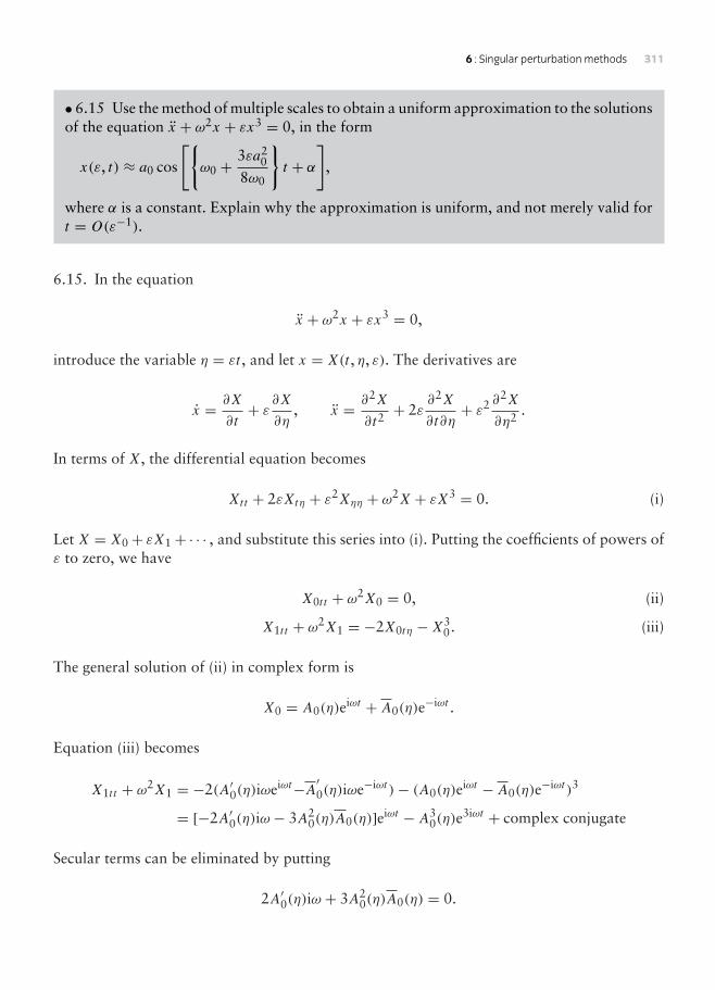
6 : Singular perturbation methods 311
• 6.15 Use the method of multiple scales to obtain a uniform approximation to the solutionsof the equation x + ω2x + εx3 = 0, in the form
x(ε, t) ≈ a0 cos
[ω0 + 3εa2
0
8ω0
t + α
],
where α is a constant. Explain why the approximation is uniform, and not merely valid fort = O(ε−1).
6.15. In the equation
x + ω2x + εx3 = 0,
introduce the variable η = εt , and let x = X(t , η, ε). The derivatives are
x = ∂X
∂t+ ε ∂X
∂η, x = ∂2X
∂t2+ 2ε
∂2X
∂t∂η+ ε2 ∂
2X
∂η2 .
In terms of X, the differential equation becomes
Xtt + 2εXtη + ε2Xηη + ω2X + εX3 = 0. (i)
Let X = X0+ εX1+ · · · , and substitute this series into (i). Putting the coefficients of powers ofε to zero, we have
X0t t + ω2X0 = 0, (ii)
X1t t + ω2X1 = −2X0tη −X30. (iii)
The general solution of (ii) in complex form is
X0 = A0(η)eiωt + A0(η)e−iωt .
Equation (iii) becomes
X1t t + ω2X1 = −2(A′0(η)iωeiωt−A′0(η)iωe−iωt )− (A0(η)eiωt − A0(η)e−iωt )3
= [−2A′0(η)iω − 3A20(η)A0(η)]eiωt − A3
0(η)e3iωt + complex conjugate
Secular terms can be eliminated by putting
2A′0(η)iω + 3A20(η)A0(η) = 0.

312 Nonlinear ordinary differential equations: problems and solutions
To solve this complex differential equation, let A0(η) = a(η)eib(η), where the functions a(η)and b(η) are real. Then
2iω(a′(η)eib(η) + ia(η)b′(η)eib(η))+ 3a(η)3eib(η) = 0,
or
[2ωia′(η)+ (3a(η)3 − 2a(η)ωb′(η))]eib(η) = 0.
The real and imaginary parts must be zero, so that
a′(η) = 0, 3a(η)3 − 2a(η)ωb′(η)) = 0.
Therefore a = 12a0, a constant, and b(η) satisfies
b′(η) = 3a20
8ω.
Hence
b(η) = 3a20
8ωη + α.
Finally
x(t) ≈ X0(t , η) = 12aei[ωt+b(η)] + 1
2ae−i[ωt+b(η)]
= a cos[ωt + b(η)] = a cos[ω + 3
8 (εa20/ω)
t + c
]
Extension of the method to higher-order multiple scales η1= εt , η2= ε2t , . . . leads to equa-tions in which the derivatives in terms of η2, . . . only appear in higher-order equations. Toorder ε the result is unaffected.
• 6.16 Use the coordinate perturbation technique to obtain the first approximation x = τ−1,t = τ + 1
2ετ(1− τ−2) to the solution of
(t + εx)x + x = 0, x(ε, 1) = 1, 0 ≤ x ≤ 1.
Confirm that the approximation is, in fact, the exact solution, and that an alternativeapproximation x = τ−1+ 1
2ετ−1, t = τ − 1
2ετ−1 is correct to order ε, for fixed τ . Construct
a graph showing the exact solution and the approximation.

6 : Singular perturbation methods 313
6.16. Use the coordinate perturbation technique to obtain the first approximation of
(t + εx)x + x = 0, x(ε, 1) = 1, 0 ≤ x ≤ 1.
Apply the straightforward approximation
x(ε, t) = x0(t)+ εx1(t)+ ε2x2(t)+ · · · , (i)
so that
t x0 + x0 = 0, (ii)
t x1 + x1 = −x0x0, (iii)
t x2 + x2 = −x0x1 − x1x0, (iv)
and so on. The boundary condition transform into the sequence of conditions
x0(1) = 1, x1(1) = 0, x2(1) = 0, . . . .
Therefore x0 = 1/t . Equation (iii) becomes
t x1 + x1 = d(tx1)
dt= 1t3
,
so that
x1 = − 12t3
+ C1
t= 1
2t
(1− 1
t2
).
From (iv)
t x2 + x2 = d(tx2)
dt= −x0x1 − x1x0 = −d(x0x1)
dt.
Therefore
ddt(tx2 + x0x1) = 0,
so that
tx2 = −x0x1 + C2 = − 12t2
(1− 1
t2
)+ C2 = − 1
2t2
(1− 1
t2
).
All these solutions are singular at t = 0.

314 Nonlinear ordinary differential equations: problems and solutions
To remove the singularities, let
t = τ + εT1(τ )+ ε2T2(τ )+ · · · .
We require expansions for inverse powers of t . Using binomial expansions,
1t= 1τ− ε T1
τ2 + ε2(T1
τ3 −T2
τ2
)+O(ε3),
1t2= 1τ2 − 2ε
T1
τ3 + ε2
(3T 2
1
τ4 − 2T2
τ3
)+O(ε3),
1t3= 1τ3 − 3ε
T1
τ4 + 3ε2
(2T 2
1
τ5 − T2
τ4
)+O(ε3).
In terms of τ ,
x0 = 1τ− ε T1
τ2 + ε2(T1
τ3 −T2
τ2
)+O(ε3),
x1 = 12τ− 1
2τ3 =12
[1τ− ε T1
τ2
]− 1
2
[1τ3 − 3ε
T1
τ4
]+O(ε2)
= 12τ
(1− 1
τ2
)− εT1
2τ2
(1− 3
τ2
)+O(ε2).
Therefore
x0 + εx1 = 1τ+ ε
[12τ
(1− 1
τ2
)− T1
τ2
]+O(ε2).
We can eliminate the O(ε) term by choosing
T1 = τ
2
(1− 1
τ2
),
in which case the approximate solution is given by
x = 1τ+O(ε2), t = τ + ετ
2
(1− 1
τ2
)+O(ε2).

6 : Singular perturbation methods 315
0.5 1t
1
2
3
x
Figure 6.3 Problem 6.16: The solid curve shows the exact solution and the dashed curve shows the approximationgiven parametrically by x ≈ (1/τ)+ (ε/(2τ)), t ≈ τ − (ε/(2τ)) with ε = 0.2
We can confirm that the approximation is, in fact, exact by substitution into the differentialequation: thus, with x = x0 + εx1,
(t + εx)x =(τ + ετ
2− ε
2τ+ ε
τ
) dxdτ
dτdt
=(τ + ετ
2+ ε
2τ
)(− 1τ2
)/(1+ ε
2+ ε
2τ
)= −1
τ= −x
as required.If we put T1 = −1/(2τ), then the approximate solution becomes
x = x0 + εx1 +O(ε2) = 1τ+ ε
2τ+O(ε2), t = τ − ε
2τ+O(ε2). (v)
Figure 6.3 shows the exact solution and the approximation given by (v).
• 6.17 Apply the method of multiple scales, with variables t and η = εt , to van der Pol’sequation x + ε(x2 − 1)x + x = 0. Show that, for t = O(ε−1),
x(ε, t) = 2a1/20 e(1/2)εt√(1+ a0eεt )
cos(t + α0)+O(ε),
where a0 and α0 are constants.
6.17. Apply the multiple scale method with η = εt to the van der Pol equation
x + ε(x2 − 1)x + x = 0.

316 Nonlinear ordinary differential equations: problems and solutions
Let x = X(t , η, ε). The derivatives are
x = ∂X
∂t+ ε ∂X
∂η, x = ∂2X
∂t2+ 2ε
∂2X
∂t∂η+ ε2 ∂
2X
∂η2 .
In terms of X, van der Pol’s equation becomes
Xtt + 2εXtη + ε2Xηη + (X2 − 1)(Xt + εXη +X) = 0. (i)
Introduce the perturbation series X = X0 + εX1 + · · · into (i) so that the first two coefficientslead to
X0t t +X0 = 0, (ii)
X1t t +X1 = −2X0tη − (X20 − 1)X0t . (iii)
In complex notation, the solution of (ii) can be expressed as
X0 = A0(η)eit + A0(η)e−it .
Equation (iii) is
X1t t +X1 = [−2iA′0(η)eit + 2iA0(η)eit ] + [2iA
′0(η)e
−it − iA0(η)e−it ]− [(A0(η)eit + A0(η)e−it )2 − 1][iA0(η)eit − iA0(η)e−it ]
= [(−2iA′0(η)+ iA0(η)− iA20A0(η))eit + (complex conjugate)]
+ (higher harmonics)
Secular terms can be eliminated if
−2A′0(η)+ A0(η)− A20A0(η) = 0.
To solve this equation, let A0(η) = a(η)eiα(η), so that
−2[a′eiα + aα′ieiα] + aeiα − a3eiα = 0,
or
[−2a′ + a − a3] + i[2aα′] = 0.
Therefore
α′ = 0, implying α = α0, a constant,
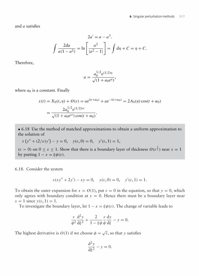
6 : Singular perturbation methods 317
and a satisfies
2a′ = a − a3.∫2da
a(1− a2)= ln
[a2
|a2 − 1|
]=
∫dη + C = η + C.
Therefore,
a = a1/20 e(1/2)η√(1+ a0eη)
,
where a0 is a constant. Finally
x(t) = X0(t , η)+O(ε) = aei(t+α0) + ae−i(t+α0) = 2A0(η) cos(t + α0)
= 2a1/20 e(1/2)εt√
(1+ a0eεt ) cos(t + α0).
• 6.18 Use the method of matched approximations to obtain a uniform approximation tothe solution of
ε(y′′ + (2/x)y′)− y = 0, y(ε, 0) = 0, y′(ε, 1) = 1,
(ε > 0) on 0 ≤ x ≤ 1. Show that there is a boundary layer of thickness O(ε12 ) near x = 1
by putting 1− x = ξφ(ε).
6.18. Consider the system
ε(xy′′ + 2y′)− xy = 0, y(ε, 0) = 0, y′(ε, 1) = 1.
To obtain the outer expansion for x = O(1), put ε = 0 in the equation, so that y = 0, whichonly agrees with boundary condition at x = 0. Hence there must be a boundary layer nearx = 1 since y(ε, 1) = 1.
To investigate the boundary layer, let 1− x = ξφ(ε). The change of variable leads to
ε
φ2
d2y
dξ2 +2
1− ξφε
φ
dydξ− y = 0.
The highest derivative is O(1) if we choose φ = √ε, so that y satisfies
d2y
dξ2 − y = 0.

318 Nonlinear ordinary differential equations: problems and solutions
to the lowest order. Therefore the inner approximation is given by
yI = Aeξ + Be−ξ = Ae(1−x)/√ε + Be−(1−x)/
√ε.
The inner approximation has to satisfy the boundary condition y′(ε, 1) = 1, so that
− A√ε+ B√
ε= 1.
Hence
yI = Ae(1−x)/√ε + (A+√ε)e−(1−x)/
√ε.
To match the inner and outer approximations, let 1− x = ηψ(ε). then we require
ψ(ε)
φ(ε)→ 0,
as ε→ 0. The choice ψ(ε) = ε will be sufficient for this purpose. Hence
yI = Aeη√ε + (A+ ε)e−η
√ε → 2A+√ε = 0,
as ε→ 0 if A = −12√ε. To summarize
yO = 0, yI = 12
√ε[e−(1−x)/
√ε − e(1−x)/
√ε] = −√ε sinh
[1− x√ε
].
• 6.19 Use the method of matched approximations to obtain a uniform approximation tothe solution of the problem
ε(y′′ + y)− y = 0, y(ε, 0) = 1, y(ε, 1) = 1, (ε > 0),
given that there are boundary layers at x = 0 and x = 1. Show that both boundary layershave thickness O(ε1/2). Compare with the exact solution.
6.19. We require a uniform approximation to the linear boundary value problem for y(x, ε)
ε(y′′ + y′)− y = 0, y(ε, 0) = 1, y(ε, 1) = 1, 0 ≤ x ≤ 1
Put ε = 0 in the equation, so that the outer approximation in the interval not near the boundariesx = 0 and x = 1 is given by yO = 0.

6 : Singular perturbation methods 319
For the inner solution yI1 near x = 0, put x = ξφ(ε), where limε→0 φ(ε) = 0. Apply thechange of variable to the differential equation:
ε
φ2
d2y
dξ2 +ε
φ
dydξ− y = 0, y(0, ε) = 1.
We choose φ = √ε so that for ε→ 0, yI satisfies
d2yI
dξ2 − yI = 0,
which has the general solution yI = Aeξ + Be−ξ . Hence, using the boundary condition,
yI1 = Aex/√ε + (1− A)e−x/
√ε.
To match this solution with the outer approximation, let x = ηε1/4 so that
yI1 = Aeη/ε1/4 + (1− A)e−η/ε1/4
.
Matching as ε→ 0 gives A = 0: therefore
yI1 = e−x/√ε.
For the inner approximation near x = 1, let x = 1− ξφ, so that
ε
φ2
d2y
dξ2 −ε
φ
dydξ− y = 0, y(0) = 1.
With φ = √ε, we get the same equation as before, so that, after matching,
yI2 = e(1−x)/√ε.
The uniform (or composite) solution is
yC = e−x/√ε + e−(1−x)/
√ε.
The given equation is second-order linear, so we can compare the exact solution yE with theapproximations above. The characteristic equation has the solutions
µ1µ2
=
−1
2 +√(
1ε+ 1
4
)−1
2 −√(
1ε+ 1
4
).

320 Nonlinear ordinary differential equations: problems and solutions
The exact solution is
yE = 1− eµ2
eµ1 − eµ2e−µ1x + eµ1 − 1
eµ1 − eµ2e−µ2x .
• 6.20 Obtain a first approximation, uniformly valid on 0 ≤ x ≤ 1, to the solution of
εy′′ + 11+ x y
′ + εy = 0, y(ε, 0) = 0, y(ε, 1) = 1.
6.20. The system is
εy′′ + 11+ x y
′ + εy = 0, y(ε, 0) = 0, y(ε, 1) = 1.
Put ε = 0 in the equation. It follows that the outer solution yO(ε, x) satisfies y′ = 0 so thatyO = 1 for all x from the boundary condition at x = 1.
For the inner solution, yI(ε, x), let x = ξφ(ε) so that the differential equation becomes
ε
φ2
d2y
dξ2 +1
1+ ξφ1φ
dydξ+ εy = 0.
Choose φ = ε and select the dominant terms. Then, the inner solution satisfies
d2yI
dξ2 +dyI
dξ= 0,
subject to y(0) = 0. Hence
yI = A(1− e−ξ ).
The outer and inner solutions match if A = 1 so that
yI = 1− e−ξ = 1− e−ξ/ε.
The uniform approximation is yC = 1− e−x/ε.
• 6.21 Apply the Lighthill technique to obtain a uniform approximation to the solution of
(t + εx)x + x = 0, x(ε, 1) = 1, 0 ≤ x ≤ 1.
(Compare Problem 6.16.)

6 : Singular perturbation methods 321
6.21. The Lighthill technique is applied to obtain a uniform approximation to the problem
(t + εx)x + x = 0, x(ε, 1) = 1, (0 ≤ x ≤ 1).
Write
x = X0(τ )+ εX1(τ )+ · · · ,t = τ + εT1(τ )+ · · · .
The differential equation becomes
[(τ + εT1 + · · · )+ ε(X0 + εX1 + · · · )](X′0 + εX′1 + · · · )(1− εT ′1 + · · · )−1
+ (X0 + εX1 + · · · ) = 0.
Therefore the perturbations satisfy
τdX0
dτ+X0 = 0, (i)
τX′1 +X1 = −X′0(T1 +X0)+ τX′0T ′1. (ii)
As in Section 2.4, the boundary condition becomes
X0(1) = 1, X1(1) = T1(1)X′0(1). (iii)
From (i) it follows that X0 = 1/τ . Equation (ii) is then
τX′1 +X1 = 1τ2T1 + 1
τ3 −1τT ′1.
Put the right-hand side equal to zero to remove singularities so that
τ2T ′1 − τT1 − 1 = 0.
The general solution of this equation is
T1 = Aτ − 12τ
.
In this case the solution of (ii) is X1 = C/τ . The second boundary condition in (iii) implies
C − (A− 12 )(−1) = 0,

322 Nonlinear ordinary differential equations: problems and solutions
so that C = −(A− 12 ). Hence the general formula for the solution is
x = 1τ− ε
τ
(A− 1
2
)ε +O(ε2), t = τ +
(Aτ − 1
2τ
)+O(ε2).
By choosing A = 12 , we can eliminate the O(ε) in x so that
x = 1τ+O(ε2), t = τ + 1
2
(τ − 1
2τ
)ε +O(ε2).
• 6.22 Obtain a first approximation, uniform on 0 ≤ x ≤ 1, to the solution of εy′ + y = x,y(ε, 0) = 1, using inner and outer approximations. Compare the exact solution and explaingeometrically why the outer approximation is independent of the boundary conditions.
6.22. The system is
εy′ + y = x, y(ε, 0) = 1.
The outer approximation is obtained by putting ε = 0, giving yO = x.To derive the inner approximation, let x = ξφ(ε), so that
ε
φ
dydξ+ y = φξ .
With φ(ε) = ε, the equation to first order reduces to
dydξ+ y = 0.
Hence y = Ae−ξ = e−ξ using the boundary condition. Therefore yI = e−x/ε,The uniform approximation is
yC = x + e−x/ε.
The exact solution of the equation is
y = x − ε + Be−x/ε = x − ε + (1+ ε)e−x/ε,
using the boundary condition y(ε, 0) = 1. If x = O(1), then the solution away from theboundary layer adjacent to x = 1 is x + O(ε provided also that the constant A = O(1)). Theboundary layer has the width O(ε). Some solutions indicating the boundary layer are shownin Figure 6.4.

6 : Singular perturbation methods 323
0.2 0.4 0.6 0.8 1x
y
–1
–0.5
0.5
1
1.5
Figure 6.4 Problem 6.22: A selection of exact solutions with ε = 0.1 and various boundary conditions.
• 6.23 Use the method of multiple scales with variables t and η = εt to show that, to a firstapproximation, the response of the van der Pol equation to a ‘soft’ forcing term describedby
x + ε(x2 − 1)x + x = εγ cosωt , ε > 0,
is the same as the unforced response, assuming that |ω| is not near 1.
6.23. The van der Pol equation with soft forcing is
x + x = ε(1− x2)x + γ cosωt,
in the non-resonant case. Let η = εt and x = X(t , η, ε). Then the derivatives become
x = ∂X
∂t+ ε ∂X
∂η, x = ∂2X
∂t2+ 2ε
∂2X
∂t∂η+ ε2 ∂
2X
∂η2 ,
and the van der Pol equation is transformed into
∂2X
∂t2+ 2ε
∂2X
∂t∂η+ ε2 ∂
2X
∂η2 +X = ε[(1− x2)
(∂X
∂t+ ε ∂X
∂η
)+ γ cosωt
].
Substitute into this equation the series X = X0+ εX1+ · · · , and equate to zero the coefficientsof like powers of ε. The first two equations are
X0t t +X0 = 0, (i)
X1t t +X1 = (1−X20)X0t + γ cosωt − 2X0tη. (ii)

324 Nonlinear ordinary differential equations: problems and solutions
Using complex notation,
X0 = A0(η)eit + A0(η)e−it .
Equation (ii) becomes
X1t t +X1 = i(A0 − A20A0 − 2A′0)e
it − i(A0 − A20A0 − 2A
′0)e
−it
− iA30e3it + iA
30e−3it + γ cosωt
The period 2π terms will be eliminated only if
A0 − A20A0 − 2A′0 = 0 (iii)
together with its conjugate. Let A0 = ρ(η)eiα(η), and substitute this form into (iii), resulting in
−2ρ′(η)− 2iρ(η)α′(η)+ ρ(η)− ρ(η)3 = 0.
The real and imaginary parts must vanish so that
2ρ′(η)− ρ(η)− ρ(η)3 = 0, α′(η) = 0.
It follows that α = α0, a constant, and that
ln
[r2
|1− r2|
]= η + C.
Hence
A(η) = eit+α0
√(1+ Ce−η)
.
Finally
x = X0(t , η)+O(ε) = 2 cos(t + tε)+ α0√(1+ Ce−εt )
+O(ε)
Significantly, X0 is independent of the angular frequency ω and the amplitude γ of the forcingoscillation, which means the response is independent of the forcing term. This will not be thecase if ω = 1.

6 : Singular perturbation methods 325
• 6.24 Repeat Problem 6.23 for x + ε(x2 − 1)x + x = cosωt , (ε > 0), where = O(1)and |ω| is not near 1. Show that
x(ε, t) =
1− ω2 cosωt +O(ε), 2 ≥ 2(1− ω2)2;
and that for 2 < 2(1− ω2)2,
x(ε, t) = 2
(1− 2
2(1− ω2)2
)1/2
cos t +
1− ω2 cosωt +O(ε).
6.24. In this problem the van der Pol equation is
x + x = ε(1− x2)x + cosωt ,
where = O(1). As in the previous problem, let η = εt and x = X(t , η, ε). The derivativesx and x in terms of X are given in the previous problem. The equations for X0 and X1 in theexpansion X = X0 + εX1 + · · · are
X0t t +X0 = cosωt , (i)
X1t t +X1 = (1−X20)X0t − 2X0tη. (ii)
The solution of (i) can be expressed in the forms
X0 = a0(η) cos t + b0(η) sin t + κ cosωt ,
where κ = /(1−ω2). Equation (ii) becomes (symbolic computation for trigonometric identitieseases the working)
X1t t +X1 = −2[a′0(η)+ b0(η)] cos t + [b′0(η)− a0(η)] sin t+ 1− (a0(η) cos t + b0(η) sin t + κ cosωt)2]× [−a0(η) sin t + b0(η) cos t − κω sinωt]
= 14 [(4− 2κ2)b0(η)− b0(η)(a0(η)
2 + b0(η)2)− 8b′0(η)] cos t
+14 [−(4− 2κ2)a0(η)+ a0(η)(a0(η)
2 + b0(η)2)+ 8a′0(η)] sin t
+ (non-secular periodic terms)
The solution for X1 is periodic if
(4− 2κ2)b0(η)− b0(η)(a0(η)2 + b0(η)
2)− 8b′0(η) = 0, (iii)
and
−(4− 2κ2)a0(η)+ a0(η)(a0(η)2 + b0(η)
2)+ 8a′0(η) = 0. (iv)

326 Nonlinear ordinary differential equations: problems and solutions
Let u0 = a20 + b2
0. Then a0×(iv)-b0×(iii) leads to the first-order equation
4du0
dη+ u2
0 − (4− 2κ2)u0 = 0.
Note that this equation always has the solution u0 = 0. This equation is separable with solution
4∫
du0
u0(u0 − λ) = −4λ
ln∣∣∣∣ u0
u0 − λ∣∣∣∣ = −
∫dη = −η + constant,
where λ = 4− 2κ2. If u0 = β when t = 0, then
u0 = λ
1+ [(λ/β)− 1]e−(1/4)λη . (v)
If λ < 0, then u0 will ultimately become negative, which is not possible: therefore the onlypossible solution in this case is u0 = 0, from which it follows that a0 = b0 = 0. Hence theforced periodic response is
x = X0 +O(ε) = κ cosωt +O(ε) =
1− ω2 cosωt +O(ε), 2 ≥ 2(1− ω2)2
If λ > 0, then u0 → λ as t →∞. From (iii), we can find b0. Using (v),
8db0
dη= λb0 − b0u0 = [b0(λ/β)− 1]e−(1/4)λη
1+ [(λ/β)− 1]e−(1/4)λη .
Integration of this separable equation leads to the solution
8 ln |b0| = 4λ
ln
[e−(1/4)λη
(λ/β − 1)+ e− 14λη
]+ C,
or
b20 =
e−(1/4)η
[(λ/β − 1)+ e−(1/4)λη]1/λ .
As t →∞, then b0 → 0, if λ > 0. From the behaviour of u0, it follows that a0 → λ. Hence theforced output of the oscillator is
x = X0 +O(ε) = 2
[1− 2
2(1− ω2)2
]1/2
cos t +
1− ω2 cosωt +O(ε),
if 2 < 2(1− ω2)2.

6 : Singular perturbation methods 327
If λ = 0, then, from (v), it follows that u0 = 0, so that a0 = b0 = 0. Hence the forcedperiodic response is
x = X0 =√
2 cosωt +O(ε).
• 6.25 Apply the matching technique to the damped pendulum equation
εx + x + sin x = 0, x(ε, 0) = 1, x(ε, 0) = 0
for ε small and positive. Show that the inner and outer approximations are given by
xI = 1, xO = 2 tan−1(e−t tan 1
2
).
(The pendulum has strong damping and strong restoring action, but the dampingdominates.)
6.25. The equation is the damped pendulum equation
εx + x + sin x = 0, x(ε, 0) = 1, x(ε, 0) = 1.
For the outer approximation xO, put ε = 0 into the equation so that xO satisfies
xO + sin xO = 0.
Hence
∫dxO
sin xO= −
∫dt = −t + C.
Integrating
ln tan(12xO) = −t + C,
so that
xO = 2 tan−1(Ae−t ).
For the inner solution, use the transformation t = εξ . The transformed equation becomes
x′′ + x′ + ε sin x = 0.
the derivatives being with respect to ξ . Putting ε = 0, the inner solution xI satisfies
x′′I + x′I = 0.

328 Nonlinear ordinary differential equations: problems and solutions
Therefore the inner solution is given by
xI = M +Ne−ξ ,
where xI(0) = 1, x′I(0) = 0. Hence M +N = 1 and N = 0. Therefore
xI = 1.
To match the outer and inner approximations, let t = η√ε. Then, expanding bothapproximations
limε→0
xO = 2 tan−1A,
limε→0
xI = 1.
Matching we find that A = tan 12 and that
xO = 2 tan−1[tan(12 )e
−t ].
• 6.26 The equation for a tidal bore on a shallow stream is
εd2η
dξ2 −dηdξ− η + η2 = 0,
where (in appropriate dimensions) η is the height of the free surface, and ξ = x − ct , wherec is the wave speed. For 0 < ε 1, find the equilibrium points for the equation and classifythem according to their linear approximations. Apply the coordinate perturbation methodto the equation for the phase paths,
εdwdη
= w + η − η2
w, where w = dη
dξ,
and show that
w = −ζ + ζ 2 +O(ε2), η = ζ − ε(−ζ + ζ 2)+O(ε2).
Confirm that, to this degree of approximation, a separatrix from the origin reaches theother equilibrium point. Interpret the result in terms of the shape of the bore.
6.26. The tidal bore equation is
εd2η
dξ2 −dηdξ− η + η2 = 0.

6 : Singular perturbation methods 329
Let w = dη/dξ . The system has two equilibrium points in the (η,w) plane, at (0, 0) and (1, 0).Near the origin η satisfies the linear approximation
εη′′ − η′ − η = 0,
which implies a saddle point. If η = 1+ η, then η has the linear approximation
εη′′ − η′ + η = 0
near (1, 0). Therefore the equilibrium point is an unstable node.The equation for the phase paths is
εdwdη
= w2 + η − η2
w. (i)
Let w = w0 + εw1 + · · · and substitute this expansion into (i) so that
ε(w0 + εw1 + · · · )(w′0 + εw′1 + · · · ) = w0 + εw1 + · · · + η − η2.
Equating coefficients of like powers of ε to zero, we obtain
w0 = η2 − η, w1 = w0w′0 = (η2 − η)(2η − 1).
Now let η = ζ + εζ1 + · · · . Then
w0 + εw1 = (ζ + εζ1)2 − (ζ + εζ1)+ ε[(ζ + εζ1)2 − (ζ + εζ1)][2(ζ + εζ1)− 1]= ζ 2 − ζ + ε[2ζ ζ1 − ζ1 + (ζ 2 − ζ )(2ζ − 1)] +O(ε2)
= ζ 2 − ζ + ε(2ζ − 1)(ζ1 + ζ 2 − ζ )+O(ε2)
The order ε term in w can be eliminated by putting ζ1 = ζ − ζ 2. We arrive at the approximatesolution given parametrically by
w = ζ 2 − ζ +O(ε2), η = ζ − ε(ζ 2 − ζ )+O(ε2). (ii)
To order ε2 this solution passes through (0, 0), where ζ = 0, and through (1, 0), whereζ = 1. In other words a phase path from the unstable node at (1, 1) becomes a separatrix ofthe saddle point at the origin as shown in Figure 6.5 with ε = 0.25. For this value of ε theapproximate phase path given by (ii) is virtually indistinguishable form the computed phasepath. The bore consists of wave advancing along a dried bed.

330 Nonlinear ordinary differential equations: problems and solutions
1–0.5 0.5 1h
–0.5
0.5
w
O P
Figure 6.5 Problem 6.26: The computed phase diagram for εη′′ − η′ − η + η2 = 0 with ε = 0.25: the separatrixjoining the node P to the saddle O is shown.
• 6.27 The function x(ε, t) satisfies the differential equation εx+xx−x = 0, (t ≥ 0) subjectto the initial conditions x(0) = 0, x(0) = 1/ε. To leading order, obtain inner and outerapproximations to the solution for small ε. Show that the composite solution is
xC = t +√2 tanh(t/(ε√
2)).
6.27. The system is
εx + xx − x = 0, x(0) = 0, x(0) = 1/ε.
The outer solution xO satisfies the equation with ε = 0, that is, xOxO − xO = 0. There are twopossible solutions; either
xO = 0, or xO = t + A. (i)
For the inner solution, let t = εξ , so that
x′′ + xx′ − εx = 0.
The inner solution xI therefore satisfies
x′′I + xIx′I = 0.
Hence
dx′IdxI
= −xI, so that x′I = −12x
2I + C.

6 : Singular perturbation methods 331
Since x′I(0) = 1 when xI = 0, it follows that C = 1. Separating the variables, we have
∫2dxI
2− x2I
=∫
dξ = ξ + B,
that is,
1√2
ln
[√2+ xI√2− xI
]= ξ + B = ξ
using the initial condition xI(0) = 0. Therefore, the inner approximation is
xI =√
2 tanh(ξ√2
)= √2 tanh
(t√ε√
2
). (ii)
To match the outer and inner approximations, let t = η√ε. In (i) try the solution xO = t+A.Then
xO = η√ε + A. (iii)
Apply the same transformation to (ii), so that
xI =√
2 tanh(ηε√
2
)= η√ε +O(ε) (iv)
for η = O(1). Expansions (iii) and (iv) match to leading order if A = 0. Hence the compositeapproximation is
xC = xO + xI = t +√
2 tanh(
t
ε√
2
).
• 6.28 Consider the initial-value problem εx+ x = e−t , x(0) = 0, x(0) = 1/ε, (0 < ε 1).Find inner and outer expansions for x, and confirm that the outer expansion to two termsis xO = 2− e−t − εe−t .
Compare computed graphs of the composite expansion and the exact solution of thedifferential equation for ε = 0.1 and for ε = 0.25.
6.28. The initial-value problem is
εx + x = e−t , x(0) = 0, x(0) = 1/ε. (i)

332 Nonlinear ordinary differential equations: problems and solutions
For the outer expansion, let xO = f0 + εf1 + · · · . Substitute this expansion into the equation,obtaining
ε(f0 + εf1 + · · · )+ (f0 + f1ε + · · · ) = e−t .
The first two coefficients satisfy
f0 = e−t , f1 = −f0.
The solutions of these equations are
f0 = −e−t + C0, f1 = −e−t + C1.
The outer expansion is therefore of the form
xO = (−e−t + C0)+ ε(−e−t + C1)+O(ε2).
For the inner expansion xI, let t = ετ . Equation (i) becomes
x′′I + x′I = εe−ετ .
Let xI = g0 + εg1 + · · · and expand eετ in powers of ε:
(g′′0 + εg′′1 + · · · )+ (g′0 + εg′1 + · · · ) = ε(1− ετ + · · · ).
The coefficients of the series satisfy
g′′0 + g′0 = 0, g′′1 + g′1 = 1.
Hence
g0 = A0 + B0e−τ , g1 = τ + A1 + B1e−τ .
The initial conditions in (i) become the sequence of conditions
gi(0) = 0 (i = 0, 1, . . . ), g′(0) = 1, g′j (0) = 0, (j = 1, 2, . . . ).
Therefore
A0 + B0 = 0, − B0 = 1, A1 + B1 = 0, − B1 + 1 = 0,
which results in A0 = 1, B0 = −1, A1 = −1, B1 = 1. The inner expansion becomes
xI = g0 + εg1 +O(ε2) = (1− e−τ )+ ε(τ − 1+ e−τ )+O(ε2).

6 : Singular perturbation methods 333
To match the outer and inner expansions, let t = ε1/2η so that τ = t/ε = ε−(1/2)η, whereη = O(1). Then
xO = [C0 + exp(−ε1/2η)] + ε[C1 + exp(−ε1/2η)] + · · ·= (C0 − 1)+ ε1/2η + ε(C1 − 1)+ · · · (ii)
Also
xI = [1− exp(−ε−(1/2)η)] + ε[ε−(1/2)η − 1+ exp(−ε−(1/2)η)] + · · ·= 1+ ε1/2η − ε + · · · , (iii)
the exponential terms being negligible as ε → 0. Comparison of (ii) with (iii) shows that theymatch to the lowest orders if C0 = 2 and C1 = 0. To summarize
xO = (2− e−t )− εe−t + · · · , (iv)
xI = (1+ t − e−t/ε)− ε(1− e−t/ε)+ · · · . (v)
For the composite solution, form
xO + xI = (2− e−t )− εe−t + (1+ t − e−t/ε)− ε(1− e−t/ε)+ · · ·
If t = O(1), then, expanding in powers of ε,
xO + xI = (3+ t − e−t )+ ε(−1− e−t )+O(ε2), (vi)
neglecting the exponential terms exp(−t/ε). Comparison of (vi) with (iv) implies that the zero-order term has the unwanted term 1 + t , and that the first-order term has the unwanted term−1. Now put t = ετ in (vi) so that
xO + xI = (2− e−ετ )− εe−ετ + (1+ ετ − e−τ )− ε(1− e−τ ).
Now assume that τ = O(1), and expand in powers of ε, so that
xO + xI = (2− e−τ )+ ε(2τ − 2+ e−τ )+ · · ·= (2+ 2t − e−t/ε)− ε(2− e−t/ε)+ · · · .
Comparison of this expansion with (v) shows the same unwanted terms; of 1 + t and −1.Therefore the composite solution is
xC = xO + xI − (1+ t)+ ε = (2− e−t − e−τ )− ε(e−t − e−τ )+ · · · .

334 Nonlinear ordinary differential equations: problems and solutions
1 2 3 4t
1
2x
Figure 6.6 Problem 6.28: The graph shows the exact solution (the dashed curve) for ε = 0.25; the outer, inner andcomposite approximations can be easily identified.
The differential equation is a linear second-order inhomogeneous equation with the exactsolution
x = 2− e−t
1− ε −1− 2ε1− ε e−t/ε.
The exact solution and the various approximations are compared in Figure 6.6 only for thecase ε = 0.25.
• 6.29 Investigate the solution of the initial/boundary-value problem
ε3x··· + εx + x + x = 0, 0 < ε 1,
with x(1) = 1, x(0) = 0, x(0) = 1/ε2 using matched approximations. Start by finding, witha regular expansion, the outer solution xO and an inner solution xI using t = ετ . Confirmthat xI cannot satisfy the conditions at t = 0. The boundary-layer thickness O(ε) at t = 0is insufficient for this problem. Hence we create an additional boundary layer of thicknessO(ε2), and a further time scale η where t = ε2η. Show that the leading order equation forthe inner–inner approximation xIIi is x′′′II +x′′II = 0, and confirm that the solution can satisfythe conditions at t = 0. Finally match the expansions xII and xI and the expansions xI andxO. Show that the approximations are
xO = e1−t , xI = e+ (1− e)e−t/ε, xII = 1− e−t/ε2
to leading order.Explain why the composite solution is
xC = e1−t + (1− e)e−t/ε − e−t/ε2.
Comparison between the numerical solution of the differential equation and the compositesolution is shown in Figure 6.10 in NODE. The composite approximation could be improvedby taking all approximations to include O(ε) terms.
6.29. Consider the third-order system
ε3x··· + εx + x + x = 0, x(1) = 1, x(0) = 0, x(0) = 1/ε2.

6 : Singular perturbation methods 335
The outer approximation xO satisfies the equation xO + xO = 0 obtained by putting ε = 0.Therefore using the condition x(1) = 1,
xO = A0e−t = e1−t . (i)
For an inner approximation try t = ετ with τ = O(1). The differential equation becomes
εx′′′ + x′′ + x′ + εx = 0
in which the derivatives are with respect to τ . The inner approximation xI(τ ) therefore satisfiesx′′I + x′I = 0, so that
xI(τ ) = A1 + B1e−τ = A1 + B1 exp(−t/ε) (iii)
for certain constants A1, B1. However, the condition x(0) = 1/ε2 cannot be satisfied by xIgiven by (ii).
This difficulty can be avoided by introducing a further, ‘inner–inner’, approximation, whichwill suit the conditions nearer to t = 0. To identify this approximation let t = ε2η, whereη = O(1). The differential equation becomes
x′′′ + x′′ + εx′ + ε3x = 0
in which the derivatives are now with respect to η. The inner–inner approximation xII(η) satsifiesx′′′II + x′′II = 0. Therefore
xII(η) = A2 + B2η + C2e−η.
The conditions at t = 0 (η = 0) require
A2 + C2 = 0, B2 − C2 = 0,
Therefore
xII = A2 + (1− A2)η − A2e−η
= A2 + (1− A2)t/ε2 − A2 exp(−t/ε2).
The factor t/ε2 →∞ as ε→ 0 for all positive t , so necessarily A2 = 0, and finally we have
xII = 1− exp(−t/ε2). (iv)
We determine the unknown constants in xI (eqn (iii)) by matching it to xO and xII overintermediate range of t . To match xI to xO put t = ε1/2q(t) in (i) and (ii), where q = O(1).

336 Nonlinear ordinary differential equations: problems and solutions
Then as ε→ 0
xO = exp(1− ε1/2q) = e+O(ε1/2),
xI = A1 + B1 exp(−q/ε1/2) = A1 + o(1).
Therefore A1 = e, and in terms of t
xI = e+ B1 exp(−t/ε).
To match xI with xII put t = e3/2p(t), where p(t) = O(1). The dominant terms match only ifB1 = 1− e. Therefore
xI = e+ (1− e) exp(−t/ε). (v)
A composite approximation, valid over the whole interval 0 < t < 1 can be constructedby considering the sum defined by xO + xI + xII on 0 < t < 1. The following table gives thedominant terms contributed by each of xO, xI and xII as ε → 0, to each of the subintervalsconsidered above.
t = O(1) but not O(ε) t = O(ε) but not O(ε2) t = O(ε2)
xO(t) e1−t e e
xI(t) e e+ (1− e)e−t/ε 1
xII(t) 1 1 1− e−t/ε2
Therefore the composite first approximation required is given by
xC = xO + xI + xII − (1+ e) = e1−t + e+ (1− e)e−t/ε + 1− e−t/ε2.
• 6.30 Let y(x, ε) satisfy εy′′ + y′ = x, where y(0, ε) = 0, y(1, ε) = 1. Find the inner andouter expansions to order ε uisng the inner variable η = x/ε. Apply the van Dyke matchingrule to show that the inner expansion is
yI ≈ (12 + ε)(1− ex/ε).
6.30. The system is
εy′′ + y′ = x, y(0, ε) = 0, y(1, ε) = 1.

6 : Singular perturbation methods 337
We require the first two terms in the outer and inner expansions. Let y = f0+ εf1+ · · · . Then
ε(f ′′0 + · · · )+ (f ′0 + εf ′1 + · · · ) = x.
Equating powers of ε, we have
f ′0 = x, f ′1 = −f ′′0 .
The boundary condition at x = 1 becomes f0(1) = 1, fi(1) = 0, (i = 1, 2, . . . ). Therefore
f0 = 12x
2 + A = 12x
2 + 12 , f1 = −x + B = −x + 1.
The outer expansion is
yO = (12x
2 + 12 )+ ε(1− x)+O(ε2). (i)
For the inner expansion, let x = εη. Then the equation becomes
y′′ + y′ = ε2η.
Let y = g0 + εg1 + · · · . Then g0 and g1 satisfy
g′′0 + g′0 = 0, g′′1 + g′1 = 0,
subject to g0(0) = 0, g1(0) = 0, . . . . Hence
g0 = C +De−η = C(1− e−η), g1 = E + F e−η = E(1− e−η),
so that the inner expansion is
yI = C(1− e−η)+ εE(1− e−η)+O(ε2). (ii)
Put x = εη in (i) where η(t) = O(1):
yO = (12ε
2η2 + 12 )+ ε(1− εη)+ · · · = 1
2 + ε + · · · . (iii)
In terms of x, yI given by (ii) becomes
yI = C(1− e−x/ε)+ εE(1− e−x/ε)+ · · · = C + εE + · · · . (iv)
Matching of (iii) and (iv) implies C = 12 and E = 1. Therefore
yI = (12 + ε)(1− e−x/ε)+ · · · .

338 Nonlinear ordinary differential equations: problems and solutions
• 6.31 In Example 6.9, a composite solution of
εd2y
dx2 + 2dydx+ y = 0, y(0) = 0, y(1) = 1,
valid over the interval 0 ≤ x ≤ 1, was found to be (eqn (6.114))
yC = e1/2(e−(1/2)x − e−2x/ε)
using matched inner and outer approximations. What linear constant coefficient second-order differential equation and boundary conditions does yC satisfy exactly?
6.31. The equation
εy′′ + 2y′ + y = 0, y(0) = 0, y(1) = 1,
has the composite solution
yC = e12 (e−(1/2)x − e−2x/ε), (i)
obtained by matched inner and outer expansions. The exponents in (i) are−12 and−2/ε, which
could arise from the characteristic equation
(m+ 12 )
(m+ 2
ε
)= 0,
which defines linearly independent solutions e−(1/2)x , e−2x/ε of the linear differential equation
2εy′′ + (ε + 4)y′ + 2y = 0.
7Forced oscillations:harmonic and subharmonicresponse, stability, andentrainment
• 7.1 Show that eqns (7.16) and (7.17), for the undamped Duffing equation in the van derPol plane have the exact solution
r2(ω2 − 1)− 3
8βr2+ 2a = constant, r = √(a2 + b2).
Show that these approximate to circles when r is large. Estimate the period on such a pathof a(t), b(t).
7.1. Equations (7.16) and (7.17) (in NODE) are
a = − 12ωb(ω2 − 1)− 3
4β(a2 + b2), (i)
b = 12ωa(ω2 − 1)− 3
4β(a2 + b2) +
2ω. (ii)
Form a × (i)+ b × (ii) which results in
d(r2)
dt= −b
ω. (iii)
where r2 = a2 + b2. From (i) and (ii)
d(r2)
da= d(r2)
dt
/dadt= − 2
ω2 − 1− 34βr
2.
Separating the variables and integrating, we have
(ω2 − 1)r2 − 38βr
4 + 2a = constant.
From (i) and (ii),dbda= −a(ω
2 − 1)− (3/4)β(a2 + b2) + b(ω2 − 1)− (3/4)β(a2 + b2) .

340 Nonlinear ordinary differential equations: problems and solutions
For r2 is large in comparison with both ω2 − 1 and , the differential equation is
dbda≈ −a
b.
Integration gives the family a2 + b2 = constant, which are concentric circles (approximately).Let δs be an increment of length on one these circles of radius r Then δs = √[(δa)2 + (δb)2].
Hence the period T is given by
T ≈∫ 2πr
0t
ds√(a2 + b2)
.
For large r,
a ≈ 3βb8ω
r2, b ≈ 3βa8ω
r2,
so that
T ≈ 8ω3βr3
∫ 2πr
0ds = 8ω
3βr3 · 2πr =16πω3βr2 .
• 7.2 Express eqns (7.16) and (7.17) in polar coordinates. Deduce the approximate periodof a(t) and b(t) for large r. Find the approximate equations for these distant paths. Showhow frequency modulation occurs, by deriving an expression for x(t).
7.2. Equations (7.16) and (7.17) (in NODE) are
a = − 12ωb(ω2 − 1)− 3
4β(a2 + b2), (i)
b = 12ωa(ω2 − 1)− 3
4β(a2 + b2) +
2ω. (ii)
Let a = r cos θ and b = r sin θ . Then
aa + bb = b
2ω,
or
drdt=
2ωsin θ . (iii)
Also
ab − ba = 12ω
[r2(ω2 − 1)− 3β
4r4 + a
].

7 : Forced oscillations 341
In polar formdθdt= 1
2ωr2
[r2(ω2 − 1)− 3β
4r4 − a
]≈ −3βr2
8ω(iv)
for r large. The polar differential equation is, from (iii) and (iv),
drdθ= dr
dt
/dθdt= −4 sin θ
3βr2 .
Therefore
3β∫r2dr = −4
∫sin θdθ ,
which can be integrated to give
r3 − 4β
cos θ = C, a constant.
which is the polar equation of phase paths in the van der Pol plane for large r. Since |4β
cos θ |is bounded, the paths will be approximately circles for large r, which agrees with the solutionof Problem 7.1.
From (iii) for a fixed and large radius, r will be constant on a path, so that, since θ changesby 2π in one circuit the period is 16πω/(3βr2). Since the frequency is 3βr2/(8ω),
x ≈ a cos t + b sin t = r[
cos
(3βr2
8ω
)t cos t + sin
(3βr2
8ω
)t sin t
]
= r cos
[(1− 3βr2
8ω
)t
].
The dependence of [1− (3βr2/(16ω))] on the radius r indicates frequency modulation of x forlarge r.
• 7.3 Consider the equation x + sgn (x) = cosωt . Assume solutions of the form x =a cosωt + b sinωt . Show that solutions of period 2π/ω exist when || ≤ 4/π . Show alsothat
a(4− πω2|a|) = π|a|, b = 0.(Hint: sgn x(t) = 4a
π√(a2 + b2)
cosωt + 4bπ√(a2 + b2)
sinωt
+higher harmonics.)

342 Nonlinear ordinary differential equations: problems and solutions
7.3. Consider the equationx + sgn (x) = cosωt .
Assume that x = a cosωt + b sinωt . We require the leading terms in the Fourier expansion of
sgn x = sgn (a cosωt + b sinωt) = A cosωt + B sinωt + · · · ,
say. Then, substituting τ = ωt ,
A = ω
π
∫ π/ω
−π/ωsgn (a cosωt + b sinωt) cosωtdt .
= 1π
∫ π
−πsgn (a cos τ + b sin τ) cos τdτ .
Let a = r cosφ, y = r sinφ so that
A = 1π
∫ π
−πsgn [r cos(τ − φ)] cos τdτ
Now cos(τ − φ) = 0 where τ = −12π + φ and τ = 1
2π + φ. Therefore
A = 1π
[−
∫ − 12π+φ
−πcos τdτ +
∫ 12π+φ
− 12π+φ
cos τdτ −∫ π
12π+φ
cos τdτ
]
= 1π[cosφ + 2 cosφ + cosφ]
= 4 cosφπ
= 4aπr
.
Similarly
B = 1π
∫ π
−πsgn [r cos(τ − φ)] sin τdτ
= 1π
[−
∫ − 12π+φ
−πsin τdτ +
∫ 12π+φ
− 12π+φ
sin τdτ −∫ π
12π+φ
sin τdτ
]
= 1π[1+ sinφ + 2 sinφ − 1+ sinφ]
= 4 sinφπ
= 4bπr
.
Hence
sgn (x) ≈ 4aπr
cosωt + 4bπr
sinωt .

7 : Forced oscillations 343
Substitute x = a cosωt + b sinωt and sgn(x) into the differential equation so that
−aω2 cosωt − bω2 sinωt + 4aπr
cosωt + 4bπr
sinωt ≈ cosωt .
The harmonics balance if
−aω2 + 4aπr
= , −bω2 + 4bπr
= 0.
From the second equation b = 0 (since r = 4/(πω2) is inconsistent with the first equation), sothat
−aω2 + 4aπ |a| = , or a(4− πω2|a|) = π|a|,
as required. For a > 0,
a = 1ω2
(4π−
).
Therefore < 4/π . Similarly, if a < 0, then > −4/π . The two inequalities can be combinedinto || < 4/π .
• 7.4 Show that solutions, period 2π , of the equation x + x3 = cos t are givenapproximately by x = a cos t , where a is a solution of 3a3 − 4a = 4.
7.4. The differential equation isx + x3 = cos t .
Assume that x ≈ a cos t + b sin t . The leading harmonics of x3 are given by
x3 = 34ar
2 cos t + 34br
2 sin t + · · · ,
where r = √(a2 + b2). The coefficients of cos t and sin t are zero if
−a + 34ar
2 = , −b + 34br
2 = 0.
The only solution of these equations is b = 0, 3a3 − 4a = 4.
• 7.5 Show that solutions, period 2π , of x+ kx+ x+ x3 = cos t are given approximatelyby x = a cos t + b sin t , where
ka − 34br
2 = 0, kb + 34ar
2 = , r = √(a2 + b2).
Deduce that the response curves are given by r2(k2 + 916r
4) = 2.

344 Nonlinear ordinary differential equations: problems and solutions
7.5. The forced Duffing-type equation is
x + kx + x + x3 = cos t . (i)
Let x ≈ a cos t + b sin t , and use the expansion
x3 = (a cos t + b sin t)3 = 34ar
2 cos t + 34br
2 sin t +higher harmonics,
where r = √(a2 + b2). Substituting the expansions into (i), we have
(−a cos t − b sin t)+ k(−a sin t + b cos t)+ (a cos t + b sin t)
+(34ar
2 cos t + 34br
2 sin t +higher harmonics) = cos t .
The first harmonics balance if
−a + kb + a + 34ar
2 = , −b − ka + b + 34br
2 = 0,
orbk + 3
4ar2 = , −ak + 3
4br2 = 0.
Squaring and adding these equations, we have the response formula
k2r2 + 916r6 = 2.
• 7.6 Obtain approximate solutions, period 2π/ω, of x+αx+βx2 = cosωt , by assumingthe form x = c + a cosωt , and deducing equations for c and a.
Show that if β is small, = O(β), and ω2 − α = O(β), then there is a solution withc ≈ −βa2/(2α) and a ≈ /(α − ω2).
7.6. Let x ≈ c + a cosωt in the equation
x + αx + βx2 = cosωt .
Use the identity
x2 = (c + a cosωt)2 = 12 (a
2 + 2c2 + 4ac cosωt + a2 cos 2ωt).
The differential equation becomes
−aω2 cosωt ++α(c + a cosωt)+ 12β(a
2 + 2c2 + 4ac cosωt + · · · ) = cosωt ,

7 : Forced oscillations 345
and the translation and first harmonic balance if
αc + 12β(a
2 + 2c2) = 0, −aω2 + αa + 2βac = . (i)
If β is small, = O(β), and ω2 − α = O(β), then assume that a = O(1) and that c =κβ +O(β2). Then
ακβ + 12βa
2 ≈ 0, −aω2 + αa ≈ .
Therefore κ = −a2/(2α), so that
c ≈ −βa2
2α, a ≈
α − ω2 .
• 7.7 Consider the equation x + x3 = cos t . Substitute x = a cos t + b sin t , and obtainthe solution x = a cos t , where 3
4a3 − a = (see Problem 7.4).
Now fit x3, by a least squares procedure, to a straight line of the form px, where p is aconstant on −A ≤ x ≤ A, so that∫ A
−A(x3 − px)2dx
is a minimum with respect to p. Deduce that this linear approximation to the restoring forceis compatible with an oscillation, period 2π , of amplitude A, provided 3
5A3 − A = .
7.7. As in Problem 7.4, the differential equation
x + x3 = cos t ,
has the approximate solution is x = a cos t , where 34a
3 − a = .In the least squares procedure, the square of the difference between z = x3 and the line
z = px over the interval −A ≤ x ≤ A is minimized to determine the slope p. The square of thedistance is
F(p) =∫ A
−A(x3 − px)2dx = 2
7A7 − 4
5A5p + 2
3A3p2.
SinceF ′(p) = −4
5A5 + 4
3pA3,
then F ′(p) is stationary where−45A
2+ 43p = 0. Therefore p = 3
5A2 and the best fit is z = 3
5A2x.
Using this approximation the equivalent linear equation is
x + 35A
2x = cos t .
This equation has the solution x = A cos t if the amplitude A is given by 35A
3 − A = .

346 Nonlinear ordinary differential equations: problems and solutions
• 7.8 Consider the equation x + 0.16x2 = 1 + 0.2 cos t . By linearizing the restoring forceabout the equilibrium points of the unforced system (without cos t), show that there aretwo modes of oscillation period 2π , given by x ≈ 2.5− cos t , x ≈ −2.5− 0.11 cos t .
Find to what extent the predicted modes differ when a substitution of the form x =c + a cos t + b sin t is used instead.
7.8. Consider the equationx + 0.16x2 = 1+ 0.2 cos t . (i)
Without the 0.2 cos t term, the unforced system has equilibrium points at 0.16x2 = 1, orx = ±2.5. Let x = ±2.5+X, but retain only linear terms inX. HenceX satisfies the approximateequation
X ± 0.8X = 0.2 cos t .
This has the periodic solutions X = K cos t , where K = −1 or K = −0.11 in the two cases.Hence the two modes of oscillation with period 2π are
x = 2.5− cos t , x = −2.5− 0.11 cos t .
An alternative method assumes that x = c + a cos t + b sin t , and uses the identity
(c + a cos t + b sin t)2 = 12 (a
2 + b2 + 2c2)+ 2ac cos t + 2bc sin t + higher harmonics.
Now balance the constant and leading harmonic terms in (i):
0.16(a2 + b2 + 2c2) = 2, −a + 0.16× 2ac = 0.2, −b + 0.16× 2cb = 0.
Since b = 0 is the only consistent solution of the third equation, it follows that a = 0.2/(−1+ 0.32c) from the second equation. Finally the first equation implies
0.16(
0.04(−1+ 0.32c)2
+ 2c2)= 2,
which after expansion becomes
0.032768c4 − 0.2048c3 + 0.1152c2 + 1.28c − 1.9936 = 0.
Numerical solution gives two real solutions c = 2.42 and c = −2.50. The corresponding valuesfor a are a = −0.89 and a = −0.11. Hence the balance method yields the solutions
x = 2.42− 0.89 cos t , x = −2.5− 0.11 cos t
for comparison with the earlier results.

7 : Forced oscillations 347
• 7.9 By examining the non-periodic solutions of the linearized equations obtained from thefirst part of Problem 7.8, show that the two solutions, period 2π , obtained are respectivelystable and unstable.
7.9. Refer back to the previous problem and the equation
x + 0.16x2 = 1+ 0.2 cos t .
The equivalent linear equations were shown to be, with x = ±2.5+X,
X ± 0.8X = 0.2 cos t .
Near x = 2.5, the transient isX = A cos(
√0.8t + α).
which is bounded: hence the solution is stable.Near x = −2.5, the transient is
X = Ae√
0.8t + Be−√
0.8t ,
which is unbounded in general: therefore the solution is unstable.
• 7.10 Show that the equations giving the equilibrium points in the van der Pol plane forsolutions period 2π/ω for the forced, damped pendulum equation
x + kx + x − 16x
3 = cosωt , k > 0
are
kωa+bω2−1+1
8 (a2+b2)
=0, −kωb+a
ω2−1+1
8 (a2+b2)
=−.
Deduce that
r2(ω2 − 1+ 1
8r2)2 + ω2k2r2 = 2, ωkr2 = b,
where r = √(a2 + b2).
7.10. The forced Duffing equation is
x + kx + x − 16x
3 = cosωt , k > 0. (i)
Let x = a cosωt + b sinωt . Then (see NODE, eqn (7.7))
x3 = 34ar
2 cosωt + 34br
2 sinωt +higher harmonics.

348 Nonlinear ordinary differential equations: problems and solutions
where r = √(a2 + b2). To the order of the first harmonics, eqn (i) becomes
(−aω2 + kbω + a − 18ar
2) cosωt + (−bω2 − kaω + b − 18br
2) sinωt ≈ cosωt .
The harmonics balance if
kωb + a(1− ω2 − 18r
2) = , (ii)
kωa − b(1− ω2 − 18r
2) = 0. (iii)
Square and add (ii) and (iii): the result is
ω2k2r2 + r2(ω2 − 1+ 18r
2)2 = 2.
Add b×(ii) to a×(iii) to give the second equation
ωkr2 = b.
• 7.11 For the equation x+ x− 16x
3= cosωt , find the frequency–amplitude equations inthe van der Pol plane. Show that there are three equilibrium points in the van der Pol planeif ω2 < 1 and || > 2
3√(8
3 )(1− ω2)3/2, and one otherwise. Investigate their stability.
7.11. The Duffing equation
x + x − 16x
3 = cosωt , (i)
is considered in NODE, Section 7.2 with β = −16 . Using the solution x = a cosωt + b sinωt ,
the frequency–amplitude equations, given by (7.16) and (7.17) are
a = − b
2ω(ω2 − 1)+ 1
8 (a2 + b2), (ii)
b = a
2ω(ω2 − 1)+ 1
8 (a2 + b2)+
2ω. (iii)
Equilibrium points in the van der Pol plane occur where b = 0 and a satisfies
(ω2 − 1)a + 18a
3 + = 0.
Let
z(a) = (ω2 − 1)a + 18a
3.

7 : Forced oscillations 349
Thenz′(a) = (ω2 − 1)+ 3
8a2.
• ω2<1. The frequency–amplitude curve in the (a, z) plane has two stationary points at
a=±√
83√(1− ω2). Correspondingly, z=∓ 2
3
√83 (1 − ω2)3/2. Therefore there are three
equilibrium points if || < 23
√83 (1−ω2)3/2, two equilibrium points if || = 2
3
√83 (1−ω2)3/2
and one otherwise.• ω2 > 1. From (ii), z(a) has no stationary points, but since z(a)→ ±∞ as a → ∞, there
will be just one equilibrium point.
Let a = a0 + a1, b = b1, where |a1| and |b1| are small, and (a0, b0) is an equilibrium point.Then the linearized equations derived from (ii) and (iii) are
a1 = − b1
2ω
(ω2 − 1)+ 1
8a2
0
,
b1 =[a0
2ω(ω2 − 1)+ 1
16ωa2
0 +
2ω
]+ a1
2ω
[(ω2 − 1)+ 3
8a2
0
]
= a1
2ω
[(ω2 − 1)+ 3
8a2
0
].
Write these equations as
a1 = −1b1, 1 = 12ω
(ω2 − 1)+ 1
8a2
0
, (iv)
b1 = 2a1, 2 = 12ω
[(ω2 − 1)+ 3
8a2
0
](v)
By elimination a1 satisfies the equation
a1 +12a1 = 0. (vi)
• ω2 > 1. From (iv) and (v),1 > 0 and2 > 0, so that (vi) implies that the only equilibriumpoint in the van der Pol plane is a centre. Therefore the corresponding periodic solution isstable.
• ω2 < 1. The curve in Figure 7.1 typically shows the curve
z(a) = (ω2 − 1)a + 18a
3
for a value of ω2 < 1. It is helpful to use the figure. The abscissae of the points on thecurve are
B : a = −√8√(1− ω2), C : a = −
√83√(1− ω2),
D : a =√
83√(1− ω2), E : a = √8
√(1− ω2).

350 Nonlinear ordinary differential equations: problems and solutions
a
z
A
B
C
D
E
F
Figure 7.1 Problem 7.11:
From (iv) and (v), we have the following results
a0 < −√
8√(1− ω2) 12 > 0 stable
−√8√(1− ω2) < a0 < −
√83√(1−2) 12 < 0 unstable
−√
83√(1− ω2) < a0 <
√83√(1−2) 12 > 0 stable√
83√(1− ω2) < a0 <
√8√(1−2) 12 < 0 unstable
a0 >√
8√(1− ω2) 12 > 0 stable
.
To summarize, the periodic solutions are stable in the intervals AE, CD and EF , andunstable in the intervals BC and DE in Figure 7.1.
• 7.12 For the equation x + αx + βx2 = cos t , substitute x = c(t)+ a(t) cos t + b(t) sin t ,and show that, neglecting a and b,
a= 12b(α−1+2βc), b=−1
2a(α−1+2βc)+,
c=−αc−βc2+ 12 (a
2+b2).Deduce that if || is large there are no solutions of period 2π , and that if α < 1 and issufficiently small there are two solutions of period 2π .
7.12. Substitute x = c(t)+ a(t) cos t + b(t) sin t into the differential equation
x + αx + βx2 = cos t ,
and neglect the second derivatives a and b. The result is
c + (2b − a) cos t − (2a + b) sin t + αc + αa cos t + αb sin t
+ β(c2 + a2 cos2 t + b2 sin2 t + 2ca cos t + 2cb sin t + 2ab sin t cos t) = cos t .

7 : Forced oscillations 351
a
c
Figure 7.2 Problem 7.12: The diagram illustrates the intersection of an ellipse and a rectangular hyperbola.
Expanding cos2 t and sin2 t , the translation and first harmonics balance if
c + αc + β(c2 + 12a
2 + 12b
2) = 0,
2b − a + αa + 2βca = ,
−2a − b + αb + 2βcb = 0.
Equilibrium occurs whereαc + β(c2 + 1
2a2 + 1
2b2) = 0, (i)
a(−1+ α + 2βc) = , (ii)
b(−1+ α + 2βc) = 0. (iii)
Assuming = 0, it follows from (ii) and (iii) that b = 0. Therefore (i) becomes
αc + β(c2 + 1
2a2
)= 0, or βa2 + 2β
(c + α
2β
)2
= α2
2β,
which is the equation of an ellipse in the (a, c) plane. Equation (ii) is the equation of a rectangularhyperbola with centre at [0, (1 − α)/(2β)]. For sufficiently large this hyperbola will notintersect the ellipse, since the ellipse is independent of . Figure 7.2 shows the intersection ofone branch of a rectangular hyperbola and an ellipse which occurs for sufficiently small.
• 7.13 Substitute x = c(t) + a(t) cos t + b(t) sin t into the equation x + αx2 = 1 + cos t(compare Problem 7.8), and show that if a and b are neglected, then
2a = b(2αc − 1), 2b = a(1− 2αc)+ , c + α(c2 + 12a
2 + 12b
2) = 1.
Use a graphical argument to show that there are two equilibrium points, when α < 14 and
<√(2/α).
7.13. Substitute x = c(t)+ a(t) cos t + b(t) sin t into the differential equation
x + αx2 = 1+ cos t ,

352 Nonlinear ordinary differential equations: problems and solutions
and neglect the second derivatives a and b. The result is
c + (2b − a) cos t − (2a + b) sin t + α(c2 + a2 cos2 t + b2 sin2 t + 2ca cos t + 2cb sin t
+ 2ab sin t cos t) = 1+ cos t
Expanding cos2 t and sin2 t , the translation and first harmonics balance if
c + α(c2 + 12a
2 + 12b
2) = 1,
2b = a − 2αca + ,
2a = −b + 2αbc,
as required. Equilibrium occurs where
α(c2 + 12a
2 + 12b
2) = 1, (i)
a − 2αca + = 0 (ii)
−b + 2αbc = 0. (iii)
From (ii) and (iii), b = 0 (assuming = 0) so that a and c satisfy
αc2 + 12αa
2 = 1, (iv)
a(2αc − 1) = . (v)
Equation (iv) represents an ellipse and (v) a rectangular hyperbola, and any equilibrium pointsoccurs where (if at all) these curves intersect. The ellipse has semi-axes
√(2/α) and 1/
√(α). The
horizontal asymptote of the hyperbola is shown in Figure 7.3. If 1/(2α)>1/√α, or α < 1
4 , thenthe curves will have at most two intersections. The lower branch of the hyperbola intersectsthe a axis at a=−. Therefore there will be two solutions for (a, c), if ≤√(2/α).
a
c
c = 1/(2a)
Figure 7.3 Problem 7.13: The diagram illustrates the intersection of an ellipse and a rectangular hyperbola.

7 : Forced oscillations 353
• 7.14 In the forced Duffing equation x+ kx+ x− 16x
3= cosωt , (k >0), substitutex= a(t) cosωt + b(t) sinωt to investigate the solutions of period 2π/ω. Assume that a andb are slowly varying and that ka, kb can be neglected. Show that the paths in the van derPol plane are given by
a = − b
2ω
ω2 − 1+ 1
8(a2 + b2)
− 1
2ka,
b = a
2ω
ω2 − 1+ 1
8(a2 + b2)
− 1
2kb +
2ω.
Show that there is one equilibrium point if ω2 > 1.Find the linear approximation in the neighbourhood of the equilibrium point when
ω2>1, and show that it is a stable node or spiral when k >0.
7.14. The forced Duffing equation is
x + kx + x − 16x
3 = cosωt . (i)
In this case, let x = a(t) cosωt + b(t) sinωt , and assume that a, b, ka and kb are small inmagnitude. Also, as in Problem 7.10,
x3 = 34ar
2 cosωt + 34br
2 sinωt + higher harmonics.
where r = √(a2 + b2). Substitute into (i) and equate to zero the coefficients of the first
harmonics: the result is
a = − b
2ω
[ω2 − 1+ 1
8r2
]− 1
2ka, (ii)
b = a
2ω
[ω2 − 1+ 1
8r2
]− 1
2kb +
2ω, (iii)
as required.Equilibrium occurs where
b[ω2 − 1+ 18r
2] + kaω = 0, (iv)
a[ω2 − 1+ 18r
2] − kbω = −. (v)
Square and add these equations:
r2[ω2 − 1+ 18r
2]2 + ω2k2r2 = 2.
Letf (r) = r2[ω2 − 1+ 1
8r2]2 + ω2k2r2

354 Nonlinear ordinary differential equations: problems and solutions
which will only be defined for r ≥ 0. It follows that
f ′(r) = 2r[ω2 − 1+ 18r
2]2 = 14r
3[ω2 − 1+ 18r
2] + 2ω2k2r.
For r > 0 and ω2 > 1, f ′(r) > 0. Therefore, for ω2 > 1, The equation f (r) = 2 has only onesolution.
Assume ω2 > 1. To linearize (ii) and (iii), let a = a0+ u and b = b0+ v, where (a0, b0) is theonly equilibrium point solution of (iv) and (v). Then the linearized approximations for u and vare
u = − u
2ω
(14a0b0 + kω
)− v
2ω
(ω2 − 1+ 1
8r20 +
14b2
0
),
v = u
2ω
(ω2 − 1+ 1
8r20 +
14a2
0
)+ v
2ω
(14a0b0 − kω
).
The equilibrium point can be classified by the method of Section 2.5. In the usual notation
p = −k < 0, q = 14ω2
[k2ω2 + (ω2 − 1+ 1
8r20 )
2 + 14r20
(ω2 − 1+ 1
8r20
)]> 0.
Hence the equilibrium point is either a stable node or spiral.
• 7.15 For the equation x + αx + βx3 = cosωt , show that the restoring force αx + βx3
is represented in the linear least-squares approximation on −A ≤ x ≤ A by (α + 35βA
2)x.Obtain the general solution of the approximating equation corresponding to a solution ofamplitude A. Deduce that there may be a subharmonic of order 1
3 if α+ 35βA
2 = 19ω
2 has areal solution A. Compare NODE, eqn (7.57) for the case when /(8α) is small. Deduce thatwhen α ≈ 1
9ω2 (close to subharmonic resonance), the subharmonic has the approximate
form
A cos(13ωt + φ)−
8αcosωt ,
where φ is a constant.(The interpretation is that when /(8α) is small enough form the oscillation to lie in
[−A,A], A can be adjusted so that the slope of the straight-line fit on [−A,A] is appropriateto the generation of a natural oscillation which is a subharmonic. The phase cannot bedetermined by this method.)
Show that the amplitude predicted for the equation x+0.15x−0.1x3=0.1 cos t isA=0.805.
7.15. The undamped forced Duffing equation is
x + αx + βx3 = cosωt .

7 : Forced oscillations 355
Consider the line z = µx. This becomes the least squares approximation to the restoring termαx + βx3 over the interval (−A,A), if µ is given by the stationary value of
F(µ) =∫ A
−A(µx − αx − βx3)dx
=∫ A
−A[(µ− α)2x2 − 2(µ− α)βx4 + β2x6]dx
= 23 (µ− α)2A3 − 4
5 (µ− α)βA5 + 27β
2A7.
DifferentiatingF ′(µ) = 4
3 (µ− α)A3 − 45A
5,
so that F ′(µ) = 0 where µ = 35A
2. The least squares approximation is z = (α + 35βA
2)x. Theequivalent linear equation using this approximation is
x +2x = cosωt , = √(α + 35βA
2).
The system could have a subharmonic if 2 = 19ω
2, or
α + 35βA
2 = 19ω
2.
A will have real solutions if α < 19ω
2. Solving the linear equation, the subharmonic will havethe approximate form
x = Acos(13ωt + φ)+
2 − ω2 cosωt .
If α ≈ 19ω
2, then 35βA
2 is small, and 2 ≈ α, so that, approximately,
x = A cos(13ωt + φ)−
8αcosωt .
The given parameter values are α=0.15, β =−0.1, =0.1 and ω=1. Then
A2 = 527β
(ω2 − 9α) = 0.648.
Hence A = 0.805.
• 7.16 Use the perturbation method to show that x+ kx+αx+βx3= cosωt has nosubharmonic of order 1
2 when β is small and k=O(β). (Assume the expansion(a cos 1
2τ + b sin 12τ + c cos τ)3= 3
4c(a2− b2)+ 3
4 (a2+ b2 + 2c2)
(a cos 12τ + b sin 1
2τ)+higher harmonics.)

356 Nonlinear ordinary differential equations: problems and solutions
7.16. In the Duffing equation
x + kx + αx + βx3 = cosωt ,
let k = κβ and τ = ωt . The equation becomes
ω2x′′ + κωβx′ + αx + βx3 = cos τ .
Let x(τ) = x0 + βx1 + · · · and ω = ω0 + βω1 + · · · , so that the differential equation becomes
(ω0 + βω1 + · · · )2(x′′0 + βx′′1 + · · · )+ κβ(ω0 + · · · )(x′0 + · · · )+ α(x0 + βx1 + · · · )+ β(x0 + βx1 + · · · )3 = cos τ
The perturbation coefficients of β in the equation vanish individually if
ω20x′′0 + αβx0 = cos τ , (i)
ω20x′′1 + αβx1 = −2ω0ω1x
′′0 − κω0x
′0 − x3
0 , (ii)
etc. For a subharmonic of frequency 12 , it follows from all these equations that α = 1
4ω20. In
this case, the general solution of (i) is
x0 = a1/2 cos 12τ + b1/2 sin 1
2τ −43ω2 cos τ .
Using the identity given in the problem, we have
− 2ω0ω1x′′0 − κω0x
′0 − x3
0 = −2ω0ω1
(−1
4a1/2 cos 12τ − 1
4b1/2 sin 12τ
)
− κω0
(−1
2a1/2 sin 12τ + 1
2b1/2 cos 12τ
)+
ω20
(a21/2 − b2
1/2)
+ 34a1/2
(a2
1/2 + b21/2 +
322
9ω40
)cos 1
2τ+34b1/2
(a2
1/2 + b21/2 +
322
9ω40
)
sin 12τ + (higher harmonics).

7 : Forced oscillations 357
The secular term can be removed by putting the coefficients of cos 12τ and sin 1
2τ in the identityequal to zero, that is,
12ω0ω1a1/2 − 1
2κω0b1/2 + 34a1/2
(a2
1/2 + b21/2 +
322
9ω40
)= 0, (iii)
12ω0ω1b1/2 + 1
2κω0a1/2 + 34b1/2
(a2
1/2 + b21/2 +
322
9ω40
)= 0. (iv)
The difference b1/2 × (iii)− a1/2 × (iv) leads to
12κω0(b
21/2 + a2
1/2) = 0,
which implies that the coefficients of subharmonic of order 12 are both zero. In which case there
can be no subharmonic of this order at least in this approximation.
• 7.17 Use the perturbation method to show that x+ kx+αx+βx3= cosωt has nosubharmonic of order other than 1
3 when β is small and k=O(β).(Use the identity
(a cos 1nτ + b sin 1
nτ + c cos τ)n = 3
4 (a2 + b2 + 2c2)(a cos τ + b sin τ)
+higher harmonics
for n = 3.)
7.17. Does the equation
x + kx + αx + βx3 = cosωt
have a subharmonic of order other than 13 when β is small and k = O(β)? Let k = κβ and
τ = ωt . The differential equation becomes
ω2x′′ + κωβx′ + αx + βx3 = cos τ .
As in Problem 7.16, let x(τ) = x0 + βx1 + · · · and ω = ω0 + βω1 + · · · . Equations (i) and (ii)of Problem 7.16 are
ω20x′′0 + αx0 = cos τ , (i)
ω20x′′1 + αx0 = −2ω0ω1x
′′0 − κω0x
′0 − x3
0 , (ii)
Look for subharmonics of order 1/n, where n = 3. Let α = ω20/n
2 so that
x0 = a1/n cos1nτ + b1/n sin
1nτ −
(n2 − 1)ω20
sin τ .

358 Nonlinear ordinary differential equations: problems and solutions
Using the identity given, the right-hand side of (ii) becomes
− 2ω0ω1x′′0 − κω0x
′0 − x3
0
= −2ω0ω1
(− 1n2 a1/n cos
1nτ − 1
nb1/n sin
1nτ
)− κω0
(−1na1/n sin
1nτ
+12b1/n cos
1nτ
)+ 3
4a1/n
(a2
1/n + b21/n +
2n42
(n2 − 1)2ω40
)cos
1nτ
+34b1/n
(a2
1/n + b21/n +
2n42
(n2 − 1)2ω20
)sin
1nτ + (higher harmonics).
The secular term can be removed by putting the coefficients of cos 1nτ and sin 1
nτ in the identity
equal to zero, that is,
2n2ω0ω1a1/n − 1
nκω0b1/n + 3
4a1/n
(a2
1/n + b21/n +
2n42
(n2 − 1)2ω40
)= 0, (iii)
2n2ω0ω1b1/n + 1
nκω0a1/n + 3
4b1/n
(a2
1/n + b21/n +
2n42
(n2 − 1)2ω40
)= 0. (iv)
The difference b1/2 × (iii)− a1/2 × (iv) leads to
12κω0(b
21/n + a2
1/n) = 0,
which imply that a1/n = b1/n = 0. Therefore there are no subharmonics except when n = 3.
• 7.18 Look for subharmonics of order 12 for the equation x+ε(x2−1)x+ x= cosωt
using the perturbation method with τ =ωt .If ω = ω0+εω1+· · · , show that this subharmonic is only possible if ω1 = 0 and 2 < 18.
(Hint: let x0 = a cos 12τ + b sin 1
2τ − 13 cos τ , and use the expansion
(x20 − 1)x′0 = 1
72 [−36+ 9(a2 + b2)+ 22](b cos 12τ − a sin 1
2τ)
+ (higher harmonics).)
7.18. The forced van der Pol equation is
x + ε(x2 − 1)x + x = cosωt .

7 : Forced oscillations 359
Apply the substitution ωt = τ so that the differential equation becomes
ω2x′′ + ωε(x2 − 1)x′ + x = cos τ .
Let x = a cosωτ + b sinωτ . Let x = x0+ εx1+· · · and ω = ω0+ εω1+· · · . The first two termsx0 and x1 satisfy
ω20x′′0 + x0 = cos τ , (i)
ω20x′′1 + x1 = −2ω0ω1x
′′0 − ω0(x
20 − 1)x′0. (ii)
From (i) there could be a subharmonic of order 12 if ω2
0 = 4, in which case the solution of (i) is
x0 = a cos 12τ + b sin 1
2τ − 13 cos τ .
The right-hand side of (ii) becomes
− 2ω0ω1x′′0 − ω0(x
20 − 1)x′0 = −2ω0ω1
(−1
4a cos 12τ − 1
4b sin 12τ
)
− ω0
b
72[−36+ 9(a2 + b2)+ 22] cos 1
2τ +a
72[36− 9(a2 + b2)
−22]sin 12τ
+ (higher harmonics).
To remove secular terms the coefficients of cos 12τ and sin τ must be zero so that
aω1 − b
36[−36+ 9(a2 + b2)+ 22] = 0,
bω1 − a
36[36− 9(a2 + b2)− 22] = 0.
Hence the only solution is
ω1 = 0, 36− 9(a2 + b2 − 22 = 0),
assuming a2 + b2 = 0. The amplitude a2 + b2 is only real if 2 < 18.

360 Nonlinear ordinary differential equations: problems and solutions
• 7.19 Extend the analysis of the equation x + ε(x2 − 1)x + x = cosωt in Problem 7.18by assuming that
x = a(t) cos 12ωt + b(t) sin 1
2ωt − 13 cosωt ,
where a and b are slowly varying. Show that when a, b, εa, εb, are neglected,12ωa = (1− 1
4ω2)b − 1
8ωa(a2 + b2 + 2
92 − 4),
12ωb = −(1− 1
4ω2)a − 1
8ωb(a2 + b2 + 2
92 − 4),
in the van der Pol plane for the subharmonic.By using ρ = a2 + b2 and φ the polar angle on the plane show that
ρ − 14ερ(ρ +K), φ = −(1− 1
4ω2)/(2ω), K = 2
92 − 4.
Deduce that
(i) When ω = 2 and K ≥ 0, all paths spiral into the origin, which is the only equilibriumpoint (so no subharmonic exists).
(ii) When ω = 2 and K ≥ 0, all paths are radial straight lines entering the origin (so thereis no subharmonic).(iii) When ω = 2 and K < 0, all paths spiral on to a limit cycle, which is a circle, radius−K and centre the origin (so x is not periodic).
(iv) When ω = 2 and K < 0, the circle center the origin and radius −K consists entirelyof equilibrium points, and all paths are radial straight lines approaching these points (eachsuch point represents a subharmonic).
(Since subharmonics are expected only in case (iv), and for a critical value of ω, entrain-ment cannot occur. For practical purposes, even if the theory were exact we could neverexpect to observe the subharmonic, though solutions near to it may occur.)
7.19. The forced van der Pol equation is
x + ε(x2 − 1)x + x = cosωt .
Let
x = a(t) cos 12ωt + b(t) sin 1
2ωt − 13 cosωt .
Neglect the terms a, b, εa and εb. Then
x ≈ (−14aω
2 + 12 bω) cos 1
2ωt + (−12 aω − 1
4bω2) sin 1
2ωt + 13ω
2 cosωt .
Also
x = (a + 12bω) cos 1
2ωt + (−12aω + b) sin 1
2ωt + 13ω sinωt .
≈ 12bω cos 1
2ωt − 12aω sin 1
2ωt + 13ω sinωt

7 : Forced oscillations 361
in the damping term. Also
ε(x2 − 1)x ≈ ε(−1
2bω + 1
8a2bω + 1
8b3ω + 1
36bω2
)cos
12ωt
+ε(
12aω − 1
8a3ω − 1
8ab2ω − 1
36aω2
)sin
12ωt
+ (higher harmonics)
We can now gather together the coefficients of cos 12ωt and sin 1
2ωt and put the coefficientsequal to zero with the result
12ωa = b(1− 1
4ω2)− 1
8ωaε(−4+ a2 + b2 + 29
2), (i)
12ωb = −a(1− 1
4ω2)− 1
8ωbε(−4+ a2 + b2 + 29
2). (ii)
Let ρ = a2 + b2. Then, using (i) and (ii),
ρ = 2aa + 2bb = −18ρ(ρ +K), (iii)
where K = 29
2 − 4. Let tanφ = b/a. Then
φ = ab − baρ
= − (1−14ω
2)
2ω. (iv)
(i) If ω = 2 and K ≥ 0, then the polar form of the equations in the van der Pol plane impliesthat the origin is the only equilibrium point, which means that there can be no subharmonicin this case. From (iii), ρ < 0 which implies that the radial distance decreases from any initialradius. For 0 < ω < 2, φ < 0, whilst for ω > 2, φ > 0. Therefore the paths in the van der Polare spirals into the origin, clockwise if ω > 2 and counterclockwise if ω < 2.
(ii) If ω = 2 and K ≥ 0, then φ = 0 and ρ < 0. Therefore the polar angles are constant andρ < 0. Hence the paths are radial and the phase direction is towards the origin. Again thereare no subharmonics.
(iii) If ω = 2 and K < 0, eqn (iii) has the solution ρ = −K which is a circle and limit cycle inthe van der Pol equation. Since ρ < 0 for ρ > K and ρ > 0 for ρ < K, the limit cycle is stable.
(iv) If ω = 2 and K < 0, all points on the circle ρ = −K are stable equilibrium points. Eachpoint corresponds to a subharmonic.
• 7.20 Given eqns (7.34), (7.41), and (7.42) (in NODE) for the response curves and thestability boundaries for the van der Pol’s equation (Figure 7.10 in NODE), eliminate r2 toshow that the boundary of the entrainment region in the γ , ν plane is given by
γ 2 = 81+ 9ν2 − (1− 3ν2)3/2/27.
for ν2 < 13 . Show that, for small ν, γ ≈ ±2ν or γ ≈ ± 2
3√
3(1− 9
8ν2).

362 Nonlinear ordinary differential equations: problems and solutions
7.20. The equation and inequalities cited for the forced van der Pol equation are
r20 ν2 + (1− 1
4r20 )
2 = γ 2, (i)
316r40 − r2
0 + 1+ ν2 > 0, (ii)
r20 ≥ 2. (iii)
where (a0, b0) is an equilibrium point in the van der Pol plane, and r0=√(a20 + b2
0). Theboundary defined by (ii) is given by
r20 = 4
3 [2±√(1− 3ν2)],
if ν2 < 13 . This equation has two positive roots (and therefore real solutions for r0) say r1 and
r2 where 0 < r21 < r
22 . It follows that inequality (ii) is satisfied if 0 < r2
0 < r21 or r2
0 > r22 .
For r0 = r2,
γ 2 = 43 [2+
√(1− 3ν2)][ν2 + 1− 2
3 2+√(1− 3ν2) + 1
9 2+√(1− 3ν2)2]
= 43 [2+
√(1− 3ν2)][23ν2 + 2
9 − 29√(1− 3ν2)]
= 827 [9ν2 + 1− (1− 3ν2)3/2].
If r0 = r1, thenγ 2 = 8
27 [9ν2 + 1+ (1− 3ν2)3/2].Figure 7.4 shows the entrainment region in the (ν, γ ). I
If |ν| is small, then
γ 2 ≈ 827
[9ν2 + 1±
(1− 9
2ν2)]
,
that isγ 2 ≈ 4ν2, or γ 2 ≈ 4
27 (4− 9ν2).
–0.5 0.5υ
11
Figure 7.4 Problem 7.20: The shaded area is the entrainment region: the upper boundary is given by γ 2 = 827 [9ν2+
1+√(1− 3ν2) and the lower boundary by γ 2 = 827 [9ν2 + 1−√(1− 3ν2)].

7 : Forced oscillations 363
Hence
γ ≈ ±2ν2, or γ ≈ 2
3√
3
(1− 9
8ν2
).
• 7.21 Consider the equation x + ε(x2 + x2 − 1)x + x = cosωt . To obtain solutions ofperiod 2π/ω, substitute x = a(t) cosωt + b(t) sinωt and deduce that, if a, b, εa, εb can beneglected, then
a = 12εa − νb − 1
4µa(a2 + b2),
b = 12ενa + b − 1
4µb(a2 + b2) + 1
2εγ ,
where
µ = 1+ 3ω2, ν = (ω2 − 1)/(εω), and γ = /(εω).Show that the stability boundaries are given by
1+ ν2 − µr2 + 116µ
2r4 = 0, 2− µr2 = 0.
7.21. The equation is
x + ε(x2 + x2 − 1)x + x = cosωt . (i)
Let x = a(t) cosωt + b(t) sinωt . Then
x = (a + ωb) cosωt + (b − aω) sinωt ,
and, neglecting a and b,
x ≈ (2ωb − aω2) cosωt − (2ωa + bω2) sinωt .
Substitution of these derivatives into (i) leads to
(2ωb − aω2) cosωt − (2ωa + bω2) sinωt + ε[(a cosωt + b sinωt)2
+ ((a + ωb) cosωt + (b − aω) sinωt)2 − 1] [(a + ωb) cosωt + (b − aω) sinωt)]+ a cosωt + b sinωt = cosωt
Neglecting εx and εb, the equation simplifies to
(2ωb − aω2) cosωt − (2ωa + bω2) sinωt + ε[(a cosωt + b sinωt)2
+ (ωb cosωt − ωa sinωt)2 − 1](ωb cosωt − aω sinωt)+ a cosωt + b sinωt
= cosωt .

364 Nonlinear ordinary differential equations: problems and solutions
The expansion of the ε term is
ε[(a cosωt + b sinωt)2 + (ωb cosωt − ωa sinωt)2 − 1](ωb cosωt − aω sinωt)
= 14εbω[−4ω + (1+ 3ω2)(a2 + b2)] cosωt+1
4εaω[4ω − (1+ 3ω2)(a2 + b2)] sinωt+ (higher harmonics).
Substitute this into the previous equation and equate the coefficients of cosωt and sinωt tozero, from which the required equations for a and b follow:
a = 12ε[a − νb − 1
4µa(a2 + b2)],
b = 12ε[νa + b − 1
4µb(a2 + b2)] + 1
2εγ ,
where µ = 1+ 3ν2, ν = (ω2 − 1)/(εω) and γ = /(εω).Equilibrium in the van der Pol plane occurs where
a − νb − 14µa(a
2 + b2) = 0, (ii)
νa + b − 14µb(a
2 + b2) = −γ . (iii)
The equations can be expressed in the form
(1− 14µr
2)a − νb = 0,
νa + (1− 14µr
2)b = −γ ,
where, after squaring and adding, r is given by
[(1− 14µr
2)2 + ν2]r2 = γ 2.
Let a = a0 and b = b0 be a solution of (i) and (ii), and consider the perturbation a = a0 + a1,b = b0 + b1, where |a1| and |b1| are small. Then, to the first order, a1 and b1 satisfy
a1 = (1− 34µa
20 − 1
4µb20)a1 − ν(1+ 1
2µa0b0)b1,
b1 = ν(1− 12a0b0)a1 + (1− 1
4µa20 − 3
4b20)b1.
Refer back to Chapter 2, Section 2.5. The solutions of the linearized equations are stable if, (inthe notation of Section 2.5),
p = 2− µr20 < 0,
and
q = (1− 34µa
20 − 1
4µb20)(1− 1
4µa20 − 3
4µb20)
+(ν − 12µa0b0)(ν + 1
2µa0b0) > 0.

7 : Forced oscillations 365
The latter inequality simplifies to
1+ ν2 − µr20 +
316µ2r4
0 > 0.
• 7.22 Show that the equation x(1−xx)+ (x2−1)x+x = 0 has an exact periodic solutionx = cost . Show that the corresponding forced equation x(1−xx)+(x2−1)x+x = cosωthas an exact solution of the from a cosωt + b sinωt , where
a(1− ω2)− ωb + ω3b(a2 + b2) = , b(1− ω2)+ ωa − ω3a(a2 + b2) = 0.
Deduce that the amplitude r = √(a2 + b2) satisfies
r2(1− ω2)2 + ω2(1− r2ω2)2 = 2.
7.22. Let x = cos t . Then
L(x) ≡ x(1− xx)+ (x2 − 1)x + x= − cos t(1+ sin t cos t)+ (sin2 t − 1)(− sin t)+ cos t = 0,
which verifies that x = cos t is an exact solution.Consider now the forced equation
L(x) = cosωt .
If x = a cosωt + b sinωt , then
L(x)− cosωt = ω2(a cosωt + b sinωt)
× [1− (a cosωt + b sinωt)(−a sinωt + b cosωt)]+ ω[ω2(−a sinωt + b cosωt)2−1](−a sinωt + b cosωt)
+ a cosωt + b sinωt − cosωt
= (1− ω2)(a cosωt + b sinωt)− ω(−a sinωt + b cosωt)
+ ω2(cosωt + b sinωt)2(−a sinωt + b cosωt)
+ ω3(− sinωt + b cosωt)3 − cosωt
= (1− ω2)(a cosωt + b sinωt)− ω(−a sinωt + b cosωt)
+ ω3(−a sinωt + b cosωt)[(a cosωt + b sinωt)2
+ (−a sinωt + b cosωt)2] − cosωt
= (1− ω2)(a cosωt + b sinωt)− ω(−a sinωt + b cosωt)
+ ω3(a2 + b2)(−a sinωt + b cosωt)− cosωt
= 0

366 Nonlinear ordinary differential equations: problems and solutions
ifa(1− ω2)− ωb + ω3b(a2 + b2) = ,
b(1− ω2)+ ωa − ω3a(a2 + b2) = 0.
These equations are equivalent tor2(1− ω2) = a,
and−ωr2 + ω3(a2 + b2) = b.
Square and add these two equations so that
r2[(1− ω2)2 + ω2(1− r2ω2)2] = 2.
• 7.23 The frequency–amplitude relation for the damped forced pendulum is (eqn (7.23)in NODE), with β =− 1
6 ) r2k2ω2 + (ω2 − 1+ 18r
2)2=2.Show that the vertex of the cusp bounding the fold in NODE, Figure 7.7 occurs where
ω = 12 √(3k2 + 4)− k√3.
Find the corresponding value for 2.
7.23. The frequency–amplitude relation for the damped forced pendulum is
r2[k2ω2 + (ω2 − 1+ 18r
2)2] = 2.
As in NODE, Section 7.3, let ρ = r2/6 and γ = /√6, so that
γ 2 = G(ρ) = ρ[k2ω2 + (ω2 − 1+ 34ρ)
2]
= 916ρ3 + 3
2(ω2 − 1)ρ2 + [k2ω2 + (ω2 − 1)2]ρ
Its derivative is
G′(ρ) = 2716ρ2 + 3(ω2 − 1)ρ + k2ω2 + (ω2 − 1)2. (i)
The equation G(ρ) = γ 2 will have three real roots if G′(ρ) = 0 has two roots for ρ ≥ 0. Thesolutions of this equation are
ρ1, ρ2 = 89 (1− ω2)± 4
9√[(1− ω2)2 − 3k2ω2].
The solutions are real and positive if
0 < ω < 1 and (1− ω2)2 > 3k2ω2.

7 : Forced oscillations 367
The two inequalities are satisfied by
0 < ω < 12 [√(3k2 + 4)− k√3].
The cusp is located atω = 1
2 [√(3k2 + 4)− k√3].
For this value of ω, ρ = 89 (1− ω2). Therefore
2 = 6γ 2 = 6G(ρ) = 6ρ[k2ω2 + (ω2 − 1+ 34ρ)
2]
= 163(1− ω2)
[k2ω2 + 1
9(1− ω2)2
]
= 64√
39
k3ω3,
where ω = 12 [√(3k2 + 4)− k√3]. In terms of k,
2 = 8√
39k3[√(3k2 + 4)−√3k]3.
• 7.24 (Combination tones) Consider the equation x+αx+βx2=1 cosω1t+2 cosω2t ,α > 0, |β| 1, where the forcing term contains two distinct frequencies ω1 and ω2. To findan approximation to the response, construct the iterative process leading to the sequenceof approximations x(0)(t), x(1)(t), . . . , and starting with
x(0) + αx(0) = 1 cosω1t + 2 cosω2t ,
x(1) + αx(1) = 1 cosω1t + 2 cosω2t − β(x(0))2,show that a particular solution is given by approximately by
x(t)=− β
2α(a2+ b2)+ a cosω1t + b cosω2t + βa2
2(4ω21 −α)
cos 2ω1t
+ βb2
2(4ω22 −α)
cos 2ω2t + βab
(ω1+ω2)2−α cos(ω1+ω2)t
+ βab
(ω1 − ω2)2 − α cos(ω1 − ω2)t ,
where a ≈ 1/(α − ω21), b ≈ 2/(α − ω2
2).(The presence of ‘sum and difference tones’ with frequenciesω1±ω2 can be detected in soundresonators having suitable nonlinear characteristics, or as an auditory illusion attributed tothe nonlinear detection mechanism in the ear (McLachlan 1956). The iterative method ofsolution can be adapted to simpler forced oscillation problems involving a single inputfrequency.)

368 Nonlinear ordinary differential equations: problems and solutions
7.24. Consider the equation
x + αx + βx2 = 1 cosω1t + 2 cosω2t , α > 0, |β| 1.
which has two forcing frequencies. Let x(0) be the first approximation, x(1) an improvedapproximation. Assume that the first approximation satisfies
x(0) + αx(0) = 1 cosω1t + 2 cosω2t .
The forced solution isx(0) = a cosω1t + b cosω2t ,
where
a = 1
α − ω21
, b = 2
α − ω22
.
Assume that x(0) is an approximation to x(1) and use it in the αx2 term. Hence x(1) satisfies
x(1) + αx(1) = 1 cosω1t + 2 cosω2t − βx(0)2
= 1 cosω1t + 2 cosω2t − β(a cosω1t + b cosω2t)2
= −12β(a
2 + b2)+ 1 cosω1t + 2 cosω2t − 12βa
2 cos 2ω1t
− 12βb
2 cos 2ω2t − βab cos(ω1 − ω2)t − βab cos(ω1 + ω2)t
This is a standard second-order linear differential equation with a constant and cosine forcingterms. Therefore
x(1) = − β
2α(a2 + b2)+ a cosω1t + b cosω2t + βa2
2(4ω21 − α)
cos 2ω1t
+ βb2
2(4ω22 − α)
cos 2ω2t + βab
(ω1 + ω2)2 − α cos(ω1 + ω2)t
+ βab
(ω1 − ω2)2 − α cos(ω1 − ω2)t ,
provided that α does not take any of the values 4ω21, 4ω2
2, (ω1 + ω2)2, or (ω1 − ω2)
2.
• 7.25 Apply the method of Problem 7.24 to the Duffing equation
x + αx + βx3 = 1 cosω1t + 2 cosω2t .

7 : Forced oscillations 369
7.25. Use the method of the previous problem for the Duffing equation
x + αx + βx3 = 1 cosω1t + 2 cosω2t .
The first approximation x(0) satisfies
x(0) + αx(0) = 1 cosω1t + 2t ,
which has the forced solution
x0 = a cosω1t + b cosω2t ,
where
a = 1
α − ω21
, b = 2
α − ω22
.
The equation for the next approximation becomes
x(1) + αx(1) = 1 cosω1t + 2 cosω2t − β(x0)3
= 1 cosω1t + 2 cosω2t − β(a cosω1t + b cosω2t)3
= (1−34β
3−32βab
2) cosω1t+(2−32βa
2b − 34βb
3) cosω2t
−14βa
3 cos 3ω1t − 14βb
3 cos 3ω2t − 34βab
2 cos(ω1 − 2ω2)t
−34βa
2b cos(2ω1 − ω2)t − 34βa
2b cos(2ω1 + ω2)t
−34βab
2 cos(ω1 + 2ω2)t .
The forced solution is
x(1) = A cosω1t + B cosω2t + C cos 3ω1t +D cos 3ω2t + E cos(ω1 − 2ω2)t
+ F cos(2ω1 − ω2)t +G cos(2ω1 + ω2)t +H cos(ω1 + 2ω2)t ,
where
A = 1 − (3/4)β3 − (3/2)βab2
α − ω21
, B = 2 − (3/2)βa2b − (3/4)βb3
α − ω2,
C = βa3
4(9ω21 − α)
, D = βb3
4(9ω22 − α)
, E = 3βab2
(ω1 − 2ω2)2 − α ,
F = 3βa2b
(2ω1 − ω2)2 − α , G = 3βa2b
(2ω1 + ω2)2 − α , H = 3βab2
(ω1 + 2ω2)2 − α .
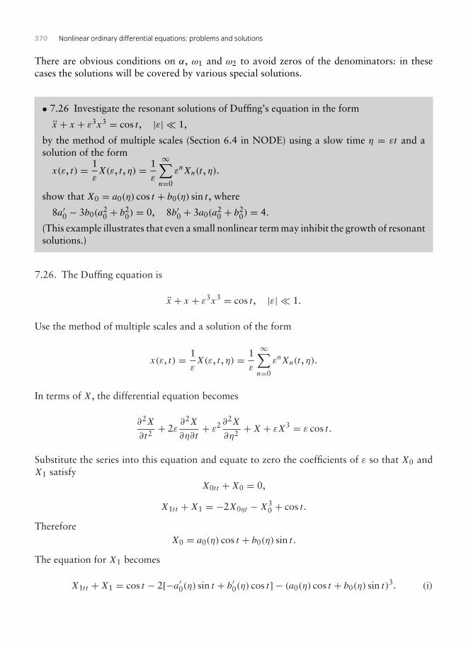
370 Nonlinear ordinary differential equations: problems and solutions
There are obvious conditions on α, ω1 and ω2 to avoid zeros of the denominators: in thesecases the solutions will be covered by various special solutions.
• 7.26 Investigate the resonant solutions of Duffing’s equation in the form
x + x + ε3x3 = cos t , |ε| 1,
by the method of multiple scales (Section 6.4 in NODE) using a slow time η = εt and asolution of the form
x(ε, t) = 1εX(ε, t , η) = 1
ε
∞∑n=0
εnXn(t , η).
show that X0 = a0(η) cos t + b0(η) sin t , where
8a′0 − 3b0(a20 + b2
0) = 0, 8b′0 + 3a0(a20 + b2
0) = 4.
(This example illustrates that even a small nonlinear term may inhibit the growth of resonantsolutions.)
7.26. The Duffing equation is
x + x + ε3x3 = cos t , |ε| 1.
Use the method of multiple scales and a solution of the form
x(ε, t) = 1εX(ε, t , η) = 1
ε
∞∑n=0
εnXn(t , η).
In terms of X, the differential equation becomes
∂2X
∂t2+ 2ε
∂2X
∂η∂t+ ε2 ∂
2X
∂η2 +X + εX3 = ε cos t .
Substitute the series into this equation and equate to zero the coefficients of ε so that X0 andX1 satisfy
X0t t +X0 = 0,
X1t t +X1 = −2X0ηt −X30 + cos t .
ThereforeX0 = a0(η) cos t + b0(η) sin t .
The equation for X1 becomes
X1t t +X1 = cos t − 2[−a′0(η) sin t + b′0(η) cos t] − (a0(η) cos t + b0(η) sin t)3. (i)

7 : Forced oscillations 371
Using the identity
(a0 cos t + b0 sin t)3 = 34a(a
2 + b2) cos t + 34b(a
2 + b2) sin t + higher harmonics,
eqn (i) is
X1t t +X1 = [1− 2b′0 − 34a0(a
20 + b2
0)] cos t +[2a′0 − 3
4b0(a20 + b2
0)]
sin t
+higher harmonics.
Secular terms disappear if the coefficients of cos t and sin t are zero, namely
1− 2b′0 − 34a0(a
20 + b2
0) = 0, 2a′0 − 34b0(a
20 + b2
0) = 0.
• 7.27 Repeat the multiple scale procedure of the previous exercise for the equation
x + x + ε3x2 = cos t , |ε| 1,
which has an unsymmetrical, quadratic departure from linearity. Use a slow time η = ε2t
and an expansion
x(ε, t) = 1ε2
∞∑n=0
εnXn(t , η).
7.27. Repeat the method of the previous problem for the equation
x + xε3x2 = cos t .
However, in this case the slow time η = ε2t . Let
x(ε, t) = 1ε2
∞∑n=0
εnXn(t , η).
In terms of X, the differential equation becomes
∂2X
∂t2+ 2ε2 ∂
2X
∂η∂t+ ε4 ∂
2X
∂η2 +X + εX2 = ε2 cos t .
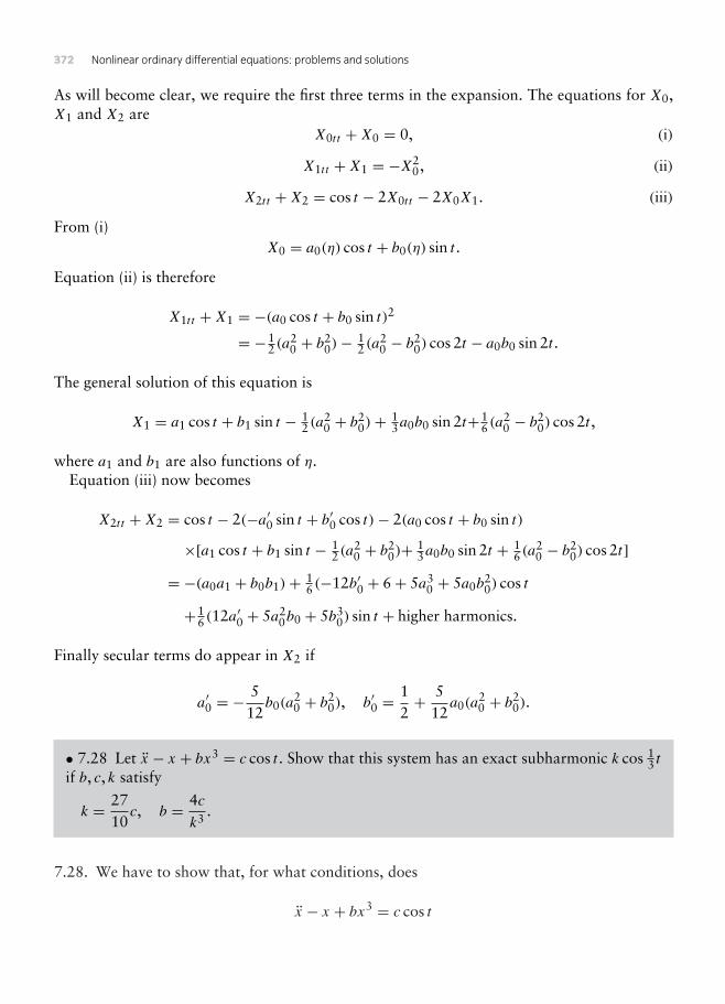
372 Nonlinear ordinary differential equations: problems and solutions
As will become clear, we require the first three terms in the expansion. The equations for X0,X1 and X2 are
X0t t +X0 = 0, (i)
X1t t +X1 = −X20, (ii)
X2t t +X2 = cos t − 2X0t t − 2X0X1. (iii)
From (i)X0 = a0(η) cos t + b0(η) sin t .
Equation (ii) is therefore
X1t t +X1 = −(a0 cos t + b0 sin t)2
= −12 (a
20 + b2
0)− 12 (a
20 − b2
0) cos 2t − a0b0 sin 2t .
The general solution of this equation is
X1 = a1 cos t + b1 sin t − 12 (a
20 + b2
0)+ 13a0b0 sin 2t+1
6 (a20 − b2
0) cos 2t ,
where a1 and b1 are also functions of η.Equation (iii) now becomes
X2t t +X2 = cos t − 2(−a′0 sin t + b′0 cos t)− 2(a0 cos t + b0 sin t)
×[a1 cos t + b1 sin t − 12 (a
20 + b2
0)+ 13a0b0 sin 2t + 1
6 (a20 − b2
0) cos 2t]= −(a0a1 + b0b1)+ 1
6 (−12b′0 + 6+ 5a30 + 5a0b
20) cos t
+16 (12a′0 + 5a2
0b0 + 5b30) sin t + higher harmonics.
Finally secular terms do appear in X2 if
a′0 = −512b0(a
20 + b2
0), b′0 =12+ 5
12a0(a
20 + b2
0).
• 7.28 Let x − x + bx3 = c cos t . Show that this system has an exact subharmonic k cos 13 t
if b, c, k satisfy
k = 2710c, b = 4c
k3 .
7.28. We have to show that, for what conditions, does
x − x + bx3 = c cos t

7 : Forced oscillations 373
have the exact subharmonic k cos 13 t . Substituting
x − x + bx3 − c cos t
= −19k cos 1
3 t − k cos 13 t + bk3 cos3 1
3 t − c cos t
= −19k cos 1
3 t − k cos 13 t + 3
4bk3 cos 1
3 t + 14k
3b cos t − c cos t
= 0
if−1
9k − k + 34bk
3 = 0, and 14bk
3 − c = 0.
Therefore k = 27c/10 and b = 4c/k3.
• 7.29 Noting that y = 0 is a solution of the second equation in the forced system
x = −x(1+ y)+ γ cos t , y = −y(x + 1),
obtain the forced periodic solution of the system.
7.29. The second equation in
x = −x(1+ y)+ γ cos t , y = −y(x + 1),
obviously has the solution y = 0. For y = 0, the first equation becomes
x = −x + γ cos t .
Let x = α cos t + β sin t . Then the first equation is satisfied if
−α sin t + β cos t = −α cos t − β sin t + γ cos t ,
that is, if−α = −β, β = −α + γ .
Therefore α = β = 12γ , so that
x = 12γ (cos t + sin t).
• 7.30 Show that, if
x = αy sin t − (x2 + y2 − 1)x, y = −αx sin t − (x2 + y2 − 1)y,
where 0 < α < π , then 2r = (r2 − 1)r. Find r as a function of t , and show that r → 1 ast →∞. Discuss the periodic oscillations which occur on the circle r = 1.

374 Nonlinear ordinary differential equations: problems and solutions
7.30. Consider the equations
x = αy sin t − (x2 + y2 − 1)x,
y = −αx sin t − (x2 + y2 − 1)y,
where 0 < α < π . Even though this is a forced system, it has an equilibrium point at the originin the phase plane. It follows that
xx + yy = 2rr = −(x2 + y2 − 1)x2 − (x2 + y2 − 1)y2
= −(r2 − 1)r2.
Separation of variables leads to
∫2dr
r(r2 − 1)= −
∫dt = −t + C.
Routine integration leads to the general solution
r2 = 11− e−(t+C)
(r2 > 1), r2 = 11+ e−(t+C)
(r2 < 1).
As t →∞, r → 1 in both cases: the circle r = 1 is a closed path in the phase plane.If r = 1, then
x = αy sin t , y = −αx sin t .
Let x = cos θ , y = sin θ . Then both equations become
θ = α sin,
which has the general solution θ = α cos t + B. Therefore
x = cos(α cos t + B), y = sin(α cos t + B).
If x = 1 at t = 0, then 1 = cos(α + B). Hence B = −α. The solutions ar then
x = cos(α cos t − α), y = sin(α sin t − α).
Solutions for x and y are shown in Figure 7.5 for the case a = 1 and the initial conditionx(0) = 1.

7 : Forced oscillations 375
5 10 15 20t
x, y
x
y
–1
–0.5
0.5
1
Figure 7.5 Problem 7.30: Solutions for x and y on the circle r = 1 with a = 1 and x(0) = 1 at t − 0.
• 7.31 Show that x+kx+x2 = cos t has an exact subharmonic of the form x = A+B cos 12 t
provided 16k2 > 1. Find A and B.
7.31. Substitute x = A+ B cos 12 t into the equation
x + kx + x2 = cos t .
Then
x + kx + x3 − cos t = −14B cos 1
2 t + k(A+ B cos 12 t)
+(A+ B cos 12 t)
2 − cos t
= (−14B + Bk) cos t + kA+ A2 + 2AB cos 1
2 t
+12B
2(1+ cos t)− cos t
= (−14B + Bk + 2AB) cos 1
2 t + kA+ A2 + 12B
2
+(12B
2 − ) cos t = 0
ifB(−1
4 + k + 2A) = 0, kA+ A2 + 12B
2 = 0, 12B
2 = .
Therefore A = 18 − 1
2k. Eliminating B2 and A:
k(18 − 1
2k)+ (18 − 1
2k)2 + = 0.
Hence = 164 (16k2 − 1), and B2 = 2 = 1
32 (16k2 − 1) provided 16k2 > 1. Subharmonics areof the form
x = (18 − 1
2k)± 14√(8k2 − 1
2 ) cos 12 t .

376 Nonlinear ordinary differential equations: problems and solutions
• 7.32 Computed solutions of the particular two-parameter Duffing equation
x + kx + x3 = cos t
have been investigated in considerable detail by Ueda (1980). Using x = a(t) cos t+b(t) sin t ,and assuming that a(t) and b(t) are slowly varying amplitudes, obtain the equations for a(t)and b(t) as in Section 7.2 (in NODE). Show that the response amplitude, r, and the forcingamplitude, , satisfy r2k2 + (1 − 3
4r2)2 = 2 for 2π -periodic solutions. By investigating
the zeros of d(2)/d(r2), show that there are three response amplitudes if 0 < k < 1/√
3.Sketch this region in the (, k) plane.
7.32. Apply the approximation x = a(t) cos t + b(t) sin t to the Duffing equation
x + kx + x3 = cos t ,
assuming that a and b and higher harmonics can be neglected. Using the result (see (7.14))
x3 = 34a(a
2 + b2) cos t + 34b(a
2 + b2) sin t + higher harmonics,
the amplitudes a and b satisfy, approximately,
(ka + 2b − a + bk + 34ar
2) cos t + (−2a + kb − ak − b + 34br
2) sin t = cos t .
where r2 = a2 + b2. The coefficients of cos t and sin t vanish if
ka + 2b − a + bk + 34ar
2 = , −2a + kb − ak − b + 34br
2 = 0.
Equilibrium in the van der Pol plane occurs where
−a + bk + 34ar
2 = , −ak − b + 34br
2 = 0.
Square and add these equations to obtain the amplitude equation
r2[k2 + (1− 34r
2)2] = 2. (i)
This equation expresses the relation between response and forcing frequencies and the damp-ing coefficient. For some values of k and , the response amplitude can take three values. Tofind where these occur, find where d()2/d(r2) = 0. Differentiating with respect to r2,
d(2)
d(r2)= k2 +
(1− 3
4r2
)2
− 32r2
(1− 3
4r2
),

7 : Forced oscillations 377
0.1 0.2 0.3 0.4 0.5k
0.1
0.2
0.3
0.4
0.5
0.6
Γ
Figure 7.6 Problem 7.32.
which is zero where
r4 − 169r2 + 16
27(k2 + 1) = 0.
The solutions are given by
r2 = 89 ± 4
9√(1− 3k2), (ii)
provided k2 ≤ 13 . Assuming that r, and k are all positive, the system has three response
amplitudes if 0 < k < 1/√
3 and one if k > 1/√
3. The relations between and k can be foundby eliminating r between eqns (i) and (ii). Computed curves are shown in Figure 7.6. The cuspis located at k = 1/
√3, where r = 2
3
√2 and = 2
√2
9√(1+ 9k2). The shaded region indicates
the three amplitude responses.
• 7.33 Show that there exists a Hamiltonian
H(x, y, t) = 12 (x
2 + y2)− 14βx
4 − x cosωt
for the undamped Duffing equation
x + x + βx3 = cosωt , x = y (see eqn (7.4))
Show also that the autonomous system for the slowly varying amplitudes a and b in thevan der Pol plane (eqns (7.16) and (7.17)) is also Hamiltonian (see Section 2.8 in NODE).What are the implications for the types of equilibrium points in the van der Pol plane?
7.33. The Duffing equation can be expressed in the form
x = X(x, y, t) = y, y = Y (x, y, t) = −x − βx3 + cosωt ,

378 Nonlinear ordinary differential equations: problems and solutions
As in Section 2.8 (with the extension to time-dependent functions) we can observe that
∂X
∂x+ ∂Y
∂y= 0,
which implies that the system is Hamiltonian. Since
X(x, y, t) = ∂H
∂y= y,
it follows that
H(x, y, t) = 12y
2 + F(x, t).
Hence
∂F
∂x= x + βx3 − cosωt ,
so that
F(x, t) = 12x
2 + 14βx
3 − x cosωt .
Finally the Hamiltonian is
H(x, y, t) = 12 (x
2 + y2)+ 14βx
4 − cosωt .
From (7.16) and (7.17) the equations for a and b in the van der Pol plane are
a = − b
2ω(ω2 − 1)− 3
4β(a2 + b2) ≡ A(a, b),
b = a
2ω(ω2 − 1)− 3
4(a2 + b2) +
2ω≡ B(a, b).
Then
∂A
∂a+ ∂B
∂b= 3βba
4ω− 3βab
4ω= 0.
Therefore the system in the van der Pol plane is also Hamiltonian (see Section 2.8). The impli-cation of this result is that the equilibrium points in the van der Pol plane must be either centresor saddle points, or higher-order versions of centres or saddle points

7 : Forced oscillations 379
• 7.34 Show that the exact solution of the equation x + x = cosωt , (ω = 1) is
x(t) = A cos t + B sin t +
1− ω2 cosωt ,
where A and B are arbitrary constants.Introduce the van der Pol variables a(t) and b(t) through
x(t) = a(t) cosωt + b(t) sinωt ,
and show that x(t) satisfies the differential equation if a(t) and b(t) satisfy
a + 2ωb + (1− ω2)a = , b − 2ωa + (1− ω2)b = 0.
Solve these equations for a and b by combining them into an equation in z = a + ib. Solvethis equation, and confirm that, although the equations for a and b contain four constants,these constants combine in such a way that the solution for x still contains just two arbitraryconstants.
7.34. The equation
x + x = cosωt , (ω = 1), (i)
has the characteristic equation m2 + 1 = 0, and the complementary function
xf = A cos t + B sin t .
A particular solution is
xp =
1− ω2 cosωt .
Hence the general solution is
x = xf + xp = A cos t + B sin t +
1− ω2 cosωt .
Let x(t) = a(t) cosωt + b(t) sinωt . Then
x = (a + ωb) cosωt + (b − ωa) sinωt , (ii)
x = (a + 2ωb − ω2a) cosωt + (b − 2ωa − ω2b) sinωt . (iii)
Substitute (ii) and (iii) into (i) and equate to zero the coefficients of cosωt and sinωt with theresults
a + 2ωb − ω2a + a = ,
b − 2ωa − ω2b + b = 0.
380 Nonlinear ordinary differential equations: problems and solutions
Let z = a + ib so that z satisfies
z− 2ωiz+ (1− ω2)z = .
The characteristic equation
λ2 − 2ωiλ+ (1− ω2) = 0,
has the solutions λ = (ω ± 1)i. A particular solution is
zp =
1− ω2 .
Therefore the general solution is
z = a + ib = A1e(ω+1)it + B1e(ω−1)it . (iv)
Let A1 = α1 + iα2 and B1 = β1 + iβ2. From (iv)
a = α1 cos(ω + 1)t − α2 sin(ω + 1)t + β1 cos(ω − 1)t − β2 sin(ω − 1)t +
1− ω2 ,
b = α2 cos(ω + 1)t + α1 sin(ω + 1)t + β2 cos(ω − 1)t + β1 sin(ω − 1)t .
Finally
x = a cosωt + b sinωt
= α1[cos(ω + 1)t cosωt + sin(ω + 1)t sinωt]+ α2[− sin(ω + 1)t cosωt + cos(ω + 1)t sinωt]+ β1[cos(ω − 1)t cosωt + sin(ω − 1)t sinωt]+ β2[− sin(ω − 1)t cosωt + cos(ω − 1)t sinωt] +
1− ω2 cosωt
= α1 cos t − α2 sin t + β1 cos t − β2 sin t +
1− ω2 cosωt
= (α1 + β1) cos t − (α2 + β2) sin t +
1− ω2 cosωt
In the final line α1+β1 are α2+β2 are the arbitrary constants A and B in the original solution.

7 : Forced oscillations 381
• 7.35 Show that the system
x + (k − x2 − x2)x + βx = cos t , (k, > 0,β = 1),
has exact harmonic solutions of the form x(t) = a cos t + b sin t , if the amplitude r =√(a2 + b2) satisfies
r2[(β − 1)2 + (k − r2)2] = 2.
By investigating the solutions of d(2)/d(r2) = 0, show that there are three harmonicsolutions for an interval of values of if k2 > 3(β − 1)2. Find this interval if k = β = 2.Draw the amplitude diagram r against in this case.
7.35. Let x = a cos t + b sin t . Then
x + (k − x2 − x2)x + βx − cos t
= −a cos t − b sin t + [k − (a cos t + b sin t)2 − (−a sin t + b cos t)2]× (−a sin t + b cos t)+ β(a cos t + b sin t)− cos t
= [−a + b(k − r2)+ βa − ] cos t + [−b − a(k − r2)+ βb] sin t = 0
if
b(k − r2)+ (β − 1)a = ,
−a(k − r2)+ (β − 1)b = 0.
Squaring and adding it follows that
r2[(β − 1)2 + (k − r2)2] = 2,
as required.The derivative
d(2)
d(r2)= (β − 1)2 + (k − r2)2 − 2r2(k − r2)
is zero where
3r4 − 4kr2 + k2 + (β − 1)2 = 0.
This quadratic equation in r2 has the solutions
r21 , r2
2 = 13 [2k ±
√k2 − 3(β − 1)2].
which are real and positive if k2 > 3(β − 1)2.

382 Nonlinear ordinary differential equations: problems and solutions
1 2
r
0.5
1
1.5
Γ
Figure 7.7 Problem 7.35: Showing the graph of 2 = r2[1+ (2− r2)2].
If k = β = 2, then2 = r2[1+ (2− r2)2].
Figure 7.7 shows the relation between and r.
• 7.36 Show that the equation x+ kx−x+ω2x2+ x2 = cosωt has exact solutions of theform x = c+ a cosωt + b sinωt , where the translation c and the amplitude r = √(a2 + b2)
satisfy
2 = r2[1+ ω2(1− 2c)2 + k2ω2] and ω2r2 = c(1− cω2).
Sketch a graph showing response amplitude r against the forcing amplitude .
7.36. Let x = c + a cosωt + b sinωt . Then
x + kx − x + ω2x2 + x2 − cosωt
= −aω2 cosωt − bω2 sinωt − kaω sinωt + kbω cosωt
− c − a cosωt − b sinωt + ω2(c + a cosωt + b sinωt)2
+ (−ωa sinωt + b cosωt)2 − cosωt
= (−aω2 + bkω − a + 2acω2 − ) cosωt + (−bω2 − akω − b + 2bcω2)
× sinωt + ω2(a2 + b2 + c2)− c = 0
if−a[1+ (1− 2c)ω2] + ωkb = , (i)
−ωka − b[1+ (1− 2c)ω2] = 0, (ii)
ω2(r2 + c2)− c = 0, (iii)
where r = √(a2 + b2). Squaring and adding (i) and (ii), we have
2 = r2[1+ ω2(1− 2c)2 + k2ω2]. (iv)
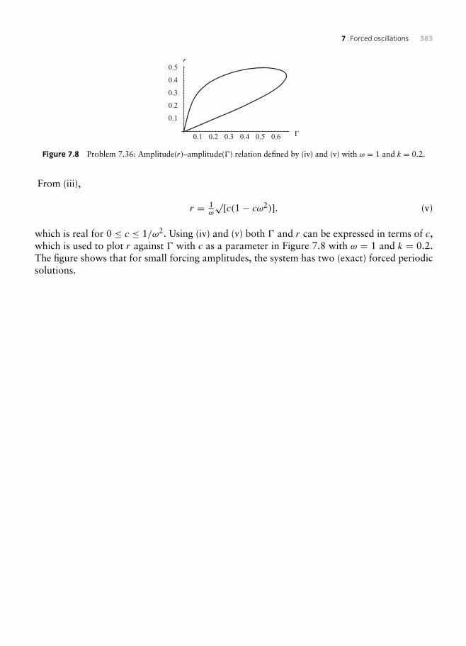
7 : Forced oscillations 383
0.1 0.2 0.3 0.4 0.5 0.6
0.1
0.2
0.3
0.4
0.5r
Γ
Figure 7.8 Problem 7.36: Amplitude(r)–amplitude() relation defined by (iv) and (v) with ω = 1 and k = 0.2.
From (iii),
r = 1ω
√[c(1− cω2)]. (v)
which is real for 0 ≤ c ≤ 1/ω2. Using (iv) and (v) both and r can be expressed in terms of c,which is used to plot r against with c as a parameter in Figure 7.8 with ω = 1 and k = 0.2.The figure shows that for small forcing amplitudes, the system has two (exact) forced periodicsolutions.

This page intentionally left blank

8 Stability
Poincaré or orbital stability is defined by Definition 8.1. A general descriptive or graphicalapproach is adopted in Problems 1–4, which are concerned with Poincaré stability.
• 8.1 Use the phase diagram for the pendulum equation x + sin x=0, to say which pathsare not Poincaré stable. (See Figure 1.2 in NODE.)
8.1. Figure 8.1 shows the phase diagram for the pendulum equation
x + sin x = 0, x = y.
Consider the stability of a typical closed path P1, within any strip bounded by two nearbyclosed paths (shown shaded). All half-paths starting in the strip remain in it for all time, so P1is Pincaré stable. The same applies to any typical path P2 in the region describing (periodic)whirling motion beyond the separatrices. The separatrices are not Poincaré stable, since thereare neighbouring half-paths that deviate unboundedly from any separatrix.
x
y
1
2
Figure 8.1 Problem 1.1(iv): Phase diagram for the pendulum equation x + sin x = 0.

386 Nonlinear ordinary differential equations: problems and solutions
• 8.2 Show that all the paths of x = x, y = y are Poincaré unstable.
8.2. The phase paths of x = x, y = y are given by y = Cx, a family of straight lines throughthe origin as shown in Figure 8.2. All paths diverge from all neighbouring paths starting fromany initial point. Therefore no paths are Poincaré or orbitally stable.
x
y
Figure 8.2 Problem 8.2: Phase diagram of x = x, y = y.
• 8.3 Find the limit cycles of the system
x = −y + x sin r, y = x + y sin r, r = √(x2 + y2).
Which cycles are Poincaré stable?
8.3. Express the equations
x = −y + x sin r, y = x + y sin r, r = √(x2 + y2),
in polar coordinates, so that
r = r sin r, θ = 1.
Limit cycles of the system are given by r = nπ , (n = 1, 2, . . . ) as shown in Figure 8.3. For(2n − 1)π < r < 2nπ , r < 0, which means that r is decreasing: for 2nπ < r < (2n + 1)π ,r > 0 and r is increasing. Since θ = 1 solutions on all paths progress progress at a constant ratein a counterclockwise sense about the origin. Hence all the limit cycles with radius (2n + 1)πare Poincaré stable since, for example, with n = 1, any path which starts in the circle C willsubsequently remain in the shaded strip.

8 : Stability 387
3 3
3
3
y
–3p p 2p 3px
c
–2–2
–3p
–2p
–p
–p p
p
2p
3p
Figure 8.3 Problem 8.3: Phase diagram for x = −y + x sin r, y = x + y sin r, r = √(x2 + y2).
• 8.4 Find the phase paths for x = x, y = y ln y, in the half-plane y > 0. Which paths arePoincaré stable?
8.4. The systemx = x, y = y ln y, (y > 0)
has equilibrium points at (0, 0) and (1, 1). The separable differential equation for the phasepaths is
dydx= y ln y
x,
which has the general solution
ln |ln y| = ln |x| + C, or y = eAx .
The phase diagram is shown in Figure 8.4. For A < 0, the phase paths all approach the x axisas x → ∞, that is they all converge to one another. Hence they are all Poincaré stable. ForA ≥ 0, all the paths diverge: hence these paths are all unstable.
–4 –2 2 4x
1
y
A > 0
A = 0
A < 0
–0.5
0.5
1.5
2
Figure 8.4 Problem 8.4: Phase diagram for x = x, y = y ln y.

388 Nonlinear ordinary differential equations: problems and solutions
• 8.5 Show that every non-zero solution of x = x is unbounded and Liapunov unstable,but that every solution of x = 1 is unbounded and stable.
8.5. Consider the one-dimensional system x = x. Its general solution is x = Aet . If A = 0, thesolution is clearly unbounded. Let x(t) = A1et and x∗(t) = A2et be two solutions with A1 andA2 both non-zero and A1 = A2. Then (adapting NODE, (8.3) to the one-dimensional case)
‖ x(t)− x∗(t) ‖ = |x(t)− x∗(t)| = |A1 − A2|et →∞,
as t →∞. Therefore all non-zero solutions are unstable in the Liapunov sense.The system x = 1 has the general solution x(t) = t + x(0): all solutions are unbounded.
Consider the stability of x∗(t) = t + x∗(0). Then
‖ x∗(t)− x(t) ‖ = |x∗(t)− x(t)| = |x∗(0)− x(0)|.
Given any ε > 0,|x∗(0)− x(0)| < ε⇒ |x∗(t)− x(t)| < ε for t > 0.
By Definition 8.2 with δ = ε, all solutions are Liapunov stable.
• 8.6 Show that the solutions of the system x = 1, y = 0, are Poincaré and Liapunov stable,but that the system x = y, y = 0 is Poincaré but not Liapunov stable.
8.6. The system x = 1, y = 0 has the general solution
x(t) = t + x(0), y(t) = y(0).
The phase diagram is shown in Figure 8.5. Consider the shaded strip which contains one of thesolutions. Any neighbouring solution which starts within the shaded region will subsequently
x
y
Figure 8.5 Problem 8.6: Phase diagram of x = 1, y = 0.

8 : Stability 389
x
y
Figure 8.6 Problem 8.6: Phase diagram of x = y, y = 0.
stay within the shaded region. Therefore all solutions are Poincaré stable. Consider the sta-bility of x∗(t) = [x∗(t), y∗(t)]. In NODE, Definition 8.2, let t0 = 0 (note that the system isautonomous). Then
‖ x(0)− x∗(0) ‖=‖ x(t)− x∗(t) ‖= √[(x(0)− x∗(0))2 + (y(0)− y(0))2].
Therefore, given any ε > 0,
‖ x∗(0)− x(0) ‖< ε⇒‖ x∗(t)− x(t) ‖< ε for t > 0,
which implies, with δ = ε, that all solutions are Liapunov stable.The system x = y, y = 0 has the general solution
x(t) = y(0)t + x(0), y(t) = y(0).
Also all points on the x axis are equilibrium points. The phase diagram is shown in Figure 8.6.The phase paths are the same as those of the first part of the problem but the sense and phasespeed are different. For the same reasons as for the previous system all solutions except theequilibrium states along y = 0 are Poincaré stable. For Liapunov stability consider
‖ x∗(t)− x(t) ‖= √[(y∗(0)t − y(0)t + x∗(0)− x(0))2 + (y∗(0)− y(0))2],
which is unbounded in t . Hence all solutions are Liapunov unstable.
• 8.7 Solve the equations x = −y(x2+y2), y = x(x2+y2), and show that the zero solutionis Liapunov stable and that all other solutions are unstable.
Replace the coordinates x,y by r,φ where x = r cos(r2t + φ), y = r sin(r2t + φ) anddeduce that r = 0, φ = 0. Show that in this coordinate system the solutions are stable.(Change of coordinates can affect the stability of a system. (See Cesari (1971, p. 12).)
8.7. Consider the system
x = −y(x2 + y2), y = x(x2 + y2).

390 Nonlinear ordinary differential equations: problems and solutions
The phase paths are given bydydx= −x
y,
which has the general solution x2 + y2 = c2: the phase paths are circles centred at the origin.Note that the origin is an equilibrium point. Substituting back into the system, we have
x = −c2y, y = c2x.
Elimination of y leads to x + c4x = 0, which has the general solution
x = α cos(c2t + β), and y = α sin(c2t + β),
where α, c and β are constants. However the three constants are not independent since
x2 + y2 = α2 = c2.
Therefore the general solution is given by
x(t) = c cos(c2t + β), y(t) = c sin(c2t + β). (i)
Observe that||x(t)|| = √[x2(t)+ y2(t)] = c. (ii)
The system is autonomous, so we need only consider the solutions for t ≥ t0 when t0 = 0 (seeDefinition 8.2(ii)).
Consider first the stability of the constant solution
x∗ = 0 = (0, 0).
Choose any ε > 0. Then, for all t ,
||x∗(t)− x(t)|| = ||0− x(t)|| = c, (iii)
and in particular||x∗(0)− x(0)|| = c. (iv)
Now choose 0 < c < ε, and in NODE, Definition 8.2, eqn (8.5), put
δ = ε (v)
for this case, given any ε > 0, we have:
if ||x∗ − x(0)|| < δ, then ||x∗(t)− x(t)|| < ε for all t .
This proves the Liapunov stability of the constant solution (0, 0).

8 : Stability 391
For other solutions, consider a solution which starts at (x0, y0). Then x0 = c cos ε andy0 = c sin ε. Hence c2 = x2
0 + y20 . The time taken for the solution to make one circuit of the
origin is 2π/(x20 +y2
0), which depends on the initial value. Hence there will always be solutionswhich start close together but do not remain so. Hence all non-zero solutions are not Liapunovstable.
Consider the change of variable (x, y)→ (r,φ) defined by
x = r cos(r2t + φ), y = r sin(r2t + φ).
Obviously r2 = x2 + y2, so that
rr = xx + yy = 0,
and, since r must be a constant in the equation for x,
−r sin(r2t + φ)(r2 + φ) = −r sin(r2t + φ)r2, or φ = 0.
The general solution is r = r0, φ = φ0. All solutions are Liapunov stable since
‖ x∗(t)− x(t) ‖ = a constant.
• 8.8 Prove that Liapunov stability of a solution implies Poincaré stability for planeautonomous systems, but not conversely: see Problem 8.6.
8.8. Briefly, NODE, Definition 8.2 for Liapunov stability for plane autonomous systems statesthat given any ε > 0, there exists a δ(ε) > 0 such that
‖ x(0)− x∗(0) ‖< δ⇒ ‖ x(t)− x∗(t) ‖< ε, (i)
for t ≥ 0, where x(t) represents any neighbouring solution. In the notation of NODE, Defini-tion 8.1 (for orbital stability), let a = x(0), a∗ = x∗ and H∗ be the half-path in the phase planedefined by x∗ for t ≥ 0. Let
q = maxx∈H
dist(x, H∗).
Then in (i),
‖ x(t)− x∗(t) ‖≤ q < ε,which establishes that Liapunov stability implies orbital stability.
The counter-example in Problem 8.6 shows that the converse cannot be true: we can havePoincaré stability without Liapunov stability.
392 Nonlinear ordinary differential equations: problems and solutions
• 8.9 Determine the stability of the solutions of
(i) x1 = x2 sin t , x2 = 0;
(ii) x1 = 0, x2 = x1 + x2.
8.9. (i) The equations x1 = x2 sin t , x2 = 0 can be expressed as
[x1x2
]=
[0 sin t0 0
] [x1x2
].
The general solution is given by
x1 = −A cos t + B, x2 = A,
and its norm is clearly bounded. By NODE, Theorems 8.9 and 8.1 the solution is Liapunovstable.(ii) The equations of the autonomous system x1 = 0, x2 = x1 + x2 has the general solution
x1 = A, x2 = −A+ Bet .
By Theorem 8.1, we need only consider the zero solution 0 = (0, 0). Consider the solution
x∗(t) = [x∗1(0),−x∗1(0)+ (x∗1(0)+ x∗2(0))et ],
which starts close to the origin. Then
‖ 0− x∗(t) ‖ =√[x∗1(0)2 + −x∗1(0)+ (x∗1(0)+ x∗2(0))et 2],
which is clearly unbounded as t →∞. Hence the system is not Liapunov stable.The phase paths are straight lines parallel to the x2 axis taken in the same sense. Hence the
paths are Poincaré stable.
• 8.10 Determine the stability of the solutions of
(i)[x1x2
]=
[ −2 11 −2
] [x1x2
]+
[1−2
]et
(ii) x + e−t x + x = et
8.10. (i) By Theorem 8.1, instead of
[x1x2
]=
[ −2 11 −2
] [x1x2
]+
[1−2
]et ,

8 : Stability 393
we need only consider
[ξ1ξ2
]=
[ −2 11 −2
] [ξ1ξ2
].
The eigenvalues of the matrix are λ1 = −1 and λ2 = −3. Therefore all solutions areasymptotically stable, which implies that the original system is also asymptotically stable.(ii) Express the equation
x + e−t x + x = et ,
in the matrix form [x
y
]=
[0 1−1 −e−t
] [x
y
]+
[0
e−t]
.
By NODE, Theorem 8.1, we need only consider the zero solution of
[ξ
η
]=
[0 1−1 −e−t
] [ξ
η
].
In the notation of NODE, Theorem 8.15, let
A =[
0 1−1 0
], C(t) =
[0 00 −e−t
].
The norm of the matrix C(t) is (see (8.21))
‖ C(t) ‖ =√e−2t = e−t .
Then, ∫ t
t0
‖ C(s) ‖ ds =∫ t
t0
e−sds = −e−t + e−t0 ,
which is bounded. Therefore by the Corollary to Theorem 8.15 all solutions are stable.
• 8.11 Show that every solution of the system x = −t2x, y = −ty is asymptotically stable.
8.11. By Theorem 8.1, the Liapunov stability of any solution of the system
x = −t2x, y = −ty

394 Nonlinear ordinary differential equations: problems and solutions
is the same as that of the zero solution. The general solution of the system is
x = Ae(1/3)t3, y = Be− 1
2 t2.
Then x → 0 and y → 0 as t → ∞. Therefore the origin is asymptotically stable as are allsolutions.
• 8.12 The motion of a heavy particle on a smooth surface of revolution with vertical axisz and shape z = f (r) in cylindrical polar coordinates is
1r4 1+ f ′2(r)
d2r
dθ2 +1r5 [rf ′(r)f ′′(r)− 21+ f ′2(r)]
(drdθ
)2
− 1r3 = −
g
h2 f′(r),
where h is the angular momentum (h = r2θ ). Show that plane, horizontal motion r = a,z = f (a), is stable for perturbations leaving h unaltered provided 3+ [af ′′(a)/f ′(a)] > 0.
8.12. The equation can be rewritten as
r1+ f ′2(r)d2r
dθ2 + [rf ′(r)f ′′(r)− 21+ f ′2(r)](
drdθ
)2
− r2 = − g
h2 r5f ′(r).
In equilibrium r = a, which means that
−a2 = − g
h2 f′(a)a5 or h2 = ga3f ′(a),
which remains constant. Substitute for h2, and consider the perturbation r = a + ρ in thedifferential equation. The linearization leads to
(a + ρ)[1+ f ′2(a)]ρ′′ − a2 − 2aρ ≈ − a2
f ′(a)[f ′(a)+ f ′′(a)ρ],
or
a[1+ f ′2(a)]ρ′′ + ρ[
3a + a2f ′′(a)f ′(a)
]= 0.
The solution for ρ is bounded and therefore stable if
3+ af ′′(a)f ′(a)
> 0.

8 : Stability 395
• 8.13 Determine the linear dependence or independence of the following:
(i) (1, 1,−1), (2, 1, 1), (0, 1,−3);
(ii) (t , 2t), (3t , 4t), (5t , 6t);
(iii) (et , e−t ), (e−t , et ). Could these both be solutions of a 2×2 homogeneous linear systems?
8.13. (i) The vectors (1, 1,−1), (2, 1, 1) and (0, 1,−3) are linearly independent since
∣∣∣∣∣∣1 1 −12 1 10 1 −3
∣∣∣∣∣∣ = 0.
(ii) The equations
α1
[t
2t
]+ α2
[3t4t
]+ α3
[5t6t
]= 0,
have the non-zero solution α1 = 2, α2 = 1 and α3 = −1 for all t . Then by Definition 8.5, thevectors are linearly dependent.(iii) The only solution of the equations
α1
[et
e−t]+ α2
[e−tet
]= 0
is α1 = α2 = 0. Hence the vectors are linearly independent.
• 8.14 Construct a fundamental matrix for the system x = y, y = −x − 2y. Deduce afundamental matrix satisfying (0) = I.
8.14. The system x = y, y = −x − 2y is equivalent to
x + 2x + x = 0.
the solution of the characteristic equation is the repeated root x = −1. Therefore, a generalsolution is
[x
y
]=
[A
−A+ B]
e−t + B[
1−1
]te−t .

396 Nonlinear ordinary differential equations: problems and solutions
Hence a fundamental matrix is (e.g. put B = 0 and put A = 0)
(t) =[
e−t te−t−e−t (1− t)e−t
].
Use NODE, Theorem 8.6, the required fundamental matrix is
(t) = (t)−1(0)
=[
e−t te−t−e−t (1− t)e−t
] [1 0−1 1
]−1
=[
e−t te−t−e−t (1− t)e−t
] [1 01 1
]
=[(1+ t)e−t te−t−te−t (1− t)e−t
]
• 8.15 Construct a fundamental matrix for the system x1 = −x1, x2 = x1 + x2 + x3,x3 = −x2.
8.15. In matrix form the system can be expressed as x1 = −x1, x2 = x1+ x2+ x3, x3 = −x2 as
x = Ax, A = −1 0 0
1 1 10 −1 0
.
The eigenvalues of A are given by
∣∣∣∣∣∣−1− λ 0 0
1 1− λ 10 −1 −λ
∣∣∣∣∣∣ = −(λ+ 1)(λ2 − λ+ 1) = 0.
Therefore the eigenvalues are given by λ=−1 and λ= 12 ±
√3
2 i. Corresponding eigenvectorsare given by:
(i) λ = −1. Let u = (u1 u2 u3)T . Then
[A − λI] = 0 0 0
1 2 10 −1 1
u1u2u3
= 0.
Choose the solution u1 = −3, u2 = 1, u3 = 1.

8 : Stability 397
(ii) λ = 12 +
√3
2 i. Let v = (v1 v2 v3)T . Then
[A − λI] =
32 −
√3
2 i 0 0
1 12 −
√3
2 i 1
0 −1 −12 −
√3
2 i
v1v2v3
= 0.
Choose the solution v1 = 0, v2 = 12 +
√3
2 i, v3 = −1.
(iii) λ = 12 −
√3
2 i. Let w = (w1 w2 w3). We can choose an eigenvector which is the conjugate
of v in (ii), namely w1 = 0, w2 = 12 −
√3
2 i, w3 = −1.Finally a fundamental matrix is (see Definition 8.6)
(t) =
e−t 0 0
e−t(
12 +
√3
2 i)
e(
12+
√3
2 i)t
(12 −
√3
2 i)
e(
12−
√3
2 i)t
−3e−t −e(
12+
√3
2 i)t −e
(12−
√3
2 i)t
.
• 8.16 Construct a fundamental matrix for the system x1 = x2, x2 = x1, and deduce thesolution satisfying x1 = 1, x2 = 0, at t = 0.
8.16. The system x1 = x2, x2 = x1 can be expressed in the form
x = Ax, where A =[
0 11 0
].
The eigenvalues of A are given by λ = ±1. Corresponding eigenvectors are r = (1, 1)T ands = (1, −1)T . Hence a fundamental matrix is
(t) =[
et e−tet −e−t
].
By NODE, Theorem 8.6, the required solution is
x(t) = (t)−1(0)x0,
where x0 = (1, 0)T . Therefore
x(t) =[
et e−tet −e−t
] [1 11 −1
]−1 [ 10
]

398 Nonlinear ordinary differential equations: problems and solutions
Therefore
x(t) =[
et e−tet −e−t
] 1
212
12 −1
2
−1 [
10
]=
[cosh tsinh t
].
• 8.17 Construct a fundamental matrix for the system x1 = x2, x2 = x3, x3 = −2x1 +x2 + 2x3, and deduce the solution of x1 = x2 + et , x2 = x3, x3 = −2x1 + x2 + 2x3, withx(0) = (1, 0, 0)T .
8.17. The matrix of coefficients for the system x1 = x2, x2 = x3, x3 = −2x1 + x2 + 2x3 isgiven by
A = 0 1 0
0 0 1−2 1 2
.
The eigenvalues of A are given by
|A − λI| =∣∣∣∣∣∣−λ 1 00 −λ 1−2 1 2− λ
∣∣∣∣∣∣ = −(λ− 1)(λ+ 1)(λ− 2) = 0.
Corresponding eigenvectors are:
• for λ1 = 1, u = (1, 1, 1)T ;• for λ2 = −1, v = (1,−1, 1)T ;• for λ3 = 2, w = (1, 2, 4)T .
A fundamental matrix for the system is therefore
(t) = et e−t e2t
et −e−t 2e2t
et e−t 4e2t
.
Use NODE, Theorem 8.13 to obtain the solution of the inhomogeneous equation
x(t) = Ax(t)+ f(t),
where f(t) = (et , 0, 0)T . We require
(0) = 1 1 1
1 −1 21 1 4
, −1(0) = 1
6
6 3 −3
2 −3 1−2 0 2
.

8 : Stability 399
Then
x(t) = (t)−1(0)(1, 0, 0)T +∫ t
0(t − s)−1(0)f(s)ds
= et e−t e2t
et −e−t 2e2t
et e−t 4e2t
1
13
−13
+∫ t
0
et−s e−t+s e2t−2s
et−s −e−t+s 2e2t−2s
et−s e−t+s 4e2t−2s
es
13es
−13es
ds
= et e−t e2t
et −e−t 2e2t
et e−t 4e2t
1
13
−13
+
∫ t
0
et + 13e−t+2s − 1
3e2t−s
et − 13e−t+2s − 2
3e2t−s
et + 13e−t+2s − 4
3e2t+s
ds
=
et + 13e−t − 1
3e2t + tet + 16 (e
t − e−t )+ 13 (e
t − e2t )
et − 13e−t − 2
3e2t + tet − 16 (e
t − e−t )+ 23 (e
t − e2t )
et + 13e−t − 4
3e2t + tet + 16 (e
t − e−t )− 43 (e
t − e2t )
=[
32et + 1
6e−t − 23e2t + tet , 3
2et − 16e−t − 4
3e2t + tet ,−16et + 1
6e−t + tet]T
• 8.18 Show that the differential equation x(n) + a1x(n−1) + · · · + anx = 0 is equivalent to
the system
x1 = x2, x2 = x3, · · ·, xn−1 = xn, xn = −anx1 − · · · − a1xn,
with x = x1. Show that the equation for the eigenvalues is
λn + a1λn−1 + · · · + an = 0.
8.18. The matrix of coefficients for the system
x1, x2 = x3, · · · , xn−1 = xn, xn = −an − · · · − a1xn,

400 Nonlinear ordinary differential equations: problems and solutions
is
A =
0 1 0 0 · · · 00 0 1 0 · · · 00 0 0 1 · · · 0· · · · · · · · · · · · · · · · · ·0 0 0 0 · · · 1−an −an−1 −an−2 −an−3 · · · −a1
.
The eigenvalues are given by
∣∣∣∣∣∣∣∣∣∣∣∣
−λ 1 0 0 · · · 00 −λ 1 0 · · · 00 0 −λ 1 · · · 0· · · · · · · · · · · · · · · · · ·0 0 0 0 · · · 1−an −an−1 −an−2 −an−3 · · · −a1 − λ
∣∣∣∣∣∣∣∣∣∣∣∣= 0.
Let Dn(λ) denote the determinant in the previous equation. Then expansion by row 1 leads to
Dn(λ) = −λDn−1(λ)+ (−1)nan. (i)
For decreasing n, we have
Dn−1(λ) = −λDn−2(λ)+ (−1)n−1an−1, (ii)
· · ·
D2(λ) = −λD1(λ)+ a2, (iii)
where D1(λ) = −a1 − λ. Now eliminate Dn−1(λ),Dn−2(λ), . . . from eqns (i) through (iii) bymultiplying successive equations by −λ, +λ and so on, and adding them. The result is
Dn(λ) = (−1)n(an + an−1λ+ · · · + a1λn−1 + λn).
The required result follows by equating Dn(λ) to zero.
• 8.19 A bird population, p(t), is governed by the differential equation p = µ(t)p − kp,where k is the death rate and µ(t) represents a variable periodic birth rate with period 1year. Derive a condition which ensures that the mean annual population remains constant.Assuming that this condition is fulfilled, does it seem likely that, in practice, the averagepopulation will remain constant? (This is asking a question about a particular kind ofstability.)

8 : Stability 401
8.19. The general solution of p = µ(t)p − kp is
p = p(0) exp[∫ t
0µ(s)dt − ks
].
If T represents the duration of one year, then the population is on average constant if
∫ T
0µ(s)ds = kT ,
where k is the constant population average.Consider a particular solution
p∗(t) = p∗(0) exp[∫ t
0µ(s)dt − ks
].
Let K = maxt∈T [∫ T
0 µ(s)ds − kT ]. Choose any ε > 0, and let δ = εe−K . Choose initialconditions such that |p(0)− p∗(0)| < δ. Then
‖ p(t)− p∗(t) ‖ = |p(t)− p∗(t)| ≤ |p(0)− p∗(0)|eK = δeK = ε.
Hence every solution is Liapunov stable.
• 8.20 Are the periodic solutions of x+sgn (x) = 0, (i) Poincaré stable, (ii) Liapunov stable?
8.20. Consider periodic solutions of x = sgn (x). The phase diagram of the system is shown inFigure 8.7. There is one equilibrium point, at the origin, and the paths are given by
y2 = C − 2x, (x > 0); y2 = C + 2x, (x < 0).
x
y
Figure 8.7 Problem 8.20: Phase diagram of x + sgn (x) = 0.

402 Nonlinear ordinary differential equations: problems and solutions
(i) Paths starting in the shaded region remain within it which implies that the phase paths arePoincaré stable.
(ii) The origin is a centre which covers the entire (x, y) plane. Hence by NODE, Section 8.4,all solutions are Liapunov stable.
• 8.21 Give a descriptive argument to show that if the index of an equilibrium point in aplane autonomous system is not unity, then the equilibrium point is not stable.
8.21. For the equilibrium point to be locally Liapunov stable the phase paths must be eitherclosed (as in a centre) or approach the equilibrium point (as for a node or spiral), all of whichhave index 1. Therefore if the index is not 1, then the equilibrium point must be unstable. Notethat the unstable spiral has index 1 but is obviously unstable in the Liapunov sense.
• 8.22 Show that the system
x = x + y − x(x2 + y2), y = −x + y − y(x2 + y2), z = −z,has a limit cycle x2 + y2 = 1, z = 0. Find the linear approximation at the origin and soconfirm that the origin is unstable. Use cylindrical polar coordinates r = √(x2 + y2), z toshow that the limit cycle is stable. Sketch the phase diagram in the x, y, z space.
8.22. The system is given by
x = x + y − z(x2 + y2), y = −x + y − y(x2 + y2), z = −z,
which has an equilibrium point at the origin. Apply polar coordinates in the (x, y) plane, sothat
2rr = 2xx + 2yy = 2[x2 + y2 − (x2 + y2)2] = 2r2(1− r2),
or
r = r(1− r2),
and
θ sec2 θ = yx − xyx2 = − r
2
x2 .
Hence θ = −1. It is obvious that r = 1 is a limit cycle which remains in the (x, y) plane, sinceit is consistent with the solution z = 0 of the third equation.

8 : Stability 403
Near the origin, the linear approximation is
x ≈ x + y, y ≈ −x + y, z = −z,
or x
y
z
=
1 1 0−1 1 00 0 −1
x
y
z
.
The eigenvalues of the matrix are given by
∣∣∣∣∣∣1− λ 1 0−1 1− λ 00 0 −1− λ
= 0,
which has the solutionsλ = −1, λ = 1± i.
Since the complex eigenvalues have positive real parts, the equilibrium point at the origin isunstable.
The equations for the phase paths in cylindrical polar coordinates (r, θ , z) are
r = r(1− r2), θ = −1, z = −z.
The general solutions are
r = 1/√(1− Ae−2t ), θ = −t + B, z = Ce−t .
Some three-dimensional phase paths are shown in Figure 8.8. The system has a stable limitcycle because all paths approach r = 1, z = 0 as t →∞.
x
y
z
Figure 8.8 Problem 8.22: Phase diagram for x = x + y − z(x2 + y2), y = −x + y − y(x2 + y2), z = −z.

404 Nonlinear ordinary differential equations: problems and solutions
• 8.23 Show that the nth-order non-autonomous system x = X(x, t) can be reduced toan (n + 1)th order autonomous system by introducing a new variable, xn+1 = t . (The(n+ 1)th order dimensional phase diagram for the modified system is of the type suggestedby Figure 8.9 (in NODE). The system has no equilibrium points.)
8.23. For the nth order system x = X(x, t), let
x = [x1, x2, · · · , xn]T , X = [X1, X2, · · · ,Xn]T .
If we introduce a further variable xn+1 and put it equal to t . Then if we define
y = [x1, x2, · · · , xn, xn+1]T , Y = [X1, X2, · · · ,Xn , 1]T ,
then the system is equivalent to the autonomous system
y = Y(y).
Since xn+1 = t , the system can have no equilibrium points.
• 8.24 Show that all phase paths of x = x − x3 are Poincaré stable except the homoclinicpaths (see Section 3.6 in NODE).
8.24. The system x = x − x3 has three equilibrium points, at (0, 0), (1, 0) and (−1, 0). Thephase paths are given by
y2 = x2 − 12x
4 + C.
The phase diagram is shown in Figure 8.9. All paths except the homoclinic paths are closed,and therefore are Poincaré stable.
–1 1x
y
–1
1
Figure 8.9 Problem 8.24: Phase diagram for x = x − x3.

8 : Stability 405
Consider any initial point on one of the homoclinic paths. Any neighbouring point noton the homoclinic path will lie on a periodic path which is either external or internal to thehomoclinic path. In terms of Definition 8.1 a radius δ cannot be found, because as t →∞ thepath periodically departs from the separatrix by a fixed amount.
• 8.25 Investigate the equilibrium points of
x = y, y = z− y − x3, z = y + x − x3.
Confirm that the origin has homoclinic paths given by
x = ±√2sech t , y = ∓√2sech 2t sinh t , z = ±√2sech t ∓√2sech 2
t sinh t .
In which directions do the solutions approach the origin as t →±∞?
8.25. The third-order system is
x = y, y = z− y − x3, z = y + x − x3. (i)
Equilibrium occurs where
y = 0, z− y − x3 = 0, y + x − x3 = 0,
at the points(0, 0, 0), (1, 0, 1), (−1, 0,−1).
• The point (0, 0, 0). The linear approximation is
x
y
z
=
0 1 0
0 −1 11 1 0
x
y
z
.
Its eigenvalues are given by
∣∣∣∣∣∣−λ 1 00 −1− λ 11 1 −λ
∣∣∣∣∣∣ = −(λ− 1)(λ+ 1)2 = 0.
Since one eigenvalue is λ = 1, the origin is an unstable equilibrium point.• The point (1, 0, 1). Let x = 1+ u, y = v, z = 1+w. Hence the linear approximation near
this point is given by u
v
w
=
0 1 0−3 −1 1−2 1 0
u
v
w
.

406 Nonlinear ordinary differential equations: problems and solutions
Its eigenvalues are given by
∣∣∣∣∣∣−λ 1 0−3 −1− λ 1−2 1 −λ
∣∣∣∣∣∣ = −(λ− 1)(λ2 + 2) = 0.,
that is, −1 and ±i√
2. The equilibrium point is stable in the form of a centre/node (but isnot asymptotically stable).
• The point (−1, 0,−1). Let x = −1 + u, y = v, z = −1 + w. The linear approximation isthe same as the previous case so that (−1, 0,−1) is also stable.
Note that on any homoclinic path of the origin, x, y, z→ 0 as t →±∞. From (i)
z− x − y = (y + x − x3)− y − (z− y − x3) = −(z− x − y),
which has the general solution z − x − y = Ke−t . Homoclinicity is only possible if K = 0, inwhich case z = x + y. In (i) eliminate z so that x and y satisfy
x = y, y = x − x3.
Therefore, after elimination of y, x satisfies x = x − x3. The homoclinic solutions are
x = ±√2sech t , y = x = ∓√2sech 2t sinh t .
Finallyz = x + y = ±√2sech t[1− tanh t].
• 8.26 By using linear approximations investigate the equilibrium points of the Lorenzequations
x = a(y − x), y = bx − y − xz, z = xy − cz,where a, b, c > 0 are constants. Show that if b ≤ 1, then the origin is the only equilibriumpoint, and that there are three equilibrium points if b > 1. Discuss the stability of the zerosolution.
8.26. The Lorenz equations are
x = a(y − x), y = bx − y − xz, z = xy − cz.
Equilibrium occurs where
y − x = 0, bx − y − xz = 0, xy − cz = 0.

8 : Stability 407
Elimination of y and z leads to
c(b − 1)x − x3 = 0,
which has the solutions x = 0, x = ±√[c(b − 1)]. Therefore the Lorenz equations have up tothree equilibrium points, at
(0, 0, 0), (√[c(b − 1)],√[c(b − 1)], b − 1), (−√[c(b − 1)],−√[c(b − 1)], b − 1).
It is clear that, if b ≤ 1, the origin is the only equilibrium point: if b > 1 there are threeequilibrium points. Near (0, 0, 0), the linearized equations are
x
y
z
=
−a a 0
b −1 00 0 −c
x
y
z
.
Its eigenvalues are given by
∣∣∣∣∣∣−a − λ a 0b −1− λ 00 0 −c − λ
∣∣∣∣∣∣ = −(λ+ c)(λ2 + aλ+ λ+ a − ab) = 0.
Therefore the eigenvalues are
−c, 12[−(a + 1)±√(a − 1)2 + 4ab].
The origin is stable if b ≤ 1, and unstable if b > 1.
• 8.27 Test the stability of the linear system
x1 = t−2x1 − 4x2 − 2x3 + t2,x2 = −x1 + t−2x2 + x3 + t ,x3 = t−2x1 − 9x2 − 4x3 + 1.
8.27. The system can be expressed in the form x = A(t)x + f(t), where
A(t) = t−2 −4 −2−1 t−2 1t−2 −9 −4
, f(t) =
t2
t
1
.

408 Nonlinear ordinary differential equations: problems and solutions
By NODE, Theorem 8.1, the stability of this system will be the same as the zero solution ofξ = A(t)ξ . With NODE, Theorem 8.15 in view, let A(t) = B+ C(t), where
B = 0 −4 −2−1 0 10 −9 −4
, C(t) =
t−2 0 0
0 t−2 0t−2 0 0
.
Hence
‖C(t)‖ = √[t−4 + t−4 + t−4] =√
3t2
.
For any t > t0 > 0, ∫ t
t0
‖C(s)‖ds = √3∫ t
t0
dss2 =
√3[
1t0− 1t
],
which is bounded in t .Also the eigenvalues of B are given by
∣∣∣∣∣∣−λ −4 −2−1 −λ 10 −9 −4− λ
∣∣∣∣∣∣ = −(1+ λ)2(2+ λ) = 0.
The eigenvalues are real and negative.Hence by Theorem 8.15 all solutions ξ and therefore x are asymptotically stable.
• 8.28 Test the stability of the solutions of the linear system
x1 = 2x1 + e−t x2 − 3x3 + et ,x2 = −2x1 + e−t x2 + x3 + 1,x3 = (4+ e−t )x1 − x2 − 4x3 + et .
8.28. The system can be expressed in the form x = A(t)x + f(t), where
A(t) = 2 e−t −3
−2 e−t 1(4+ e−t ) −1 −4
, f(t) =
et
1et
.
By NODE, Theorem 8.1, the stability of this system will be the same as the zero solution ofξ = A(t)ξ . With NODE, Theorem 8.15 in view, let A(t) = B+ C(t), where
B = 2 0 −3−2 0 14 −1 −4
, C(t) =
0 e−t 0
0 e−t 0e−t 0 0
.

8 : Stability 409
Hence‖ C(t) ‖= √[e−2t + e−2t + e−2t ] = √3e−t .
Then for any t0, ∫ t
t0
‖ C(s) ‖ ds = √3∫ t
t0
e−sds = √3[e−t0 − e−t ],
which is bounded in t . Also the eigenvalues of B are given by
∣∣∣∣∣∣2− λ 0 −3−2 −λ 14 −1 −4− λ
∣∣∣∣∣∣ = −(1+ λ)(4+ λ+ λ2).
Therefore the eigenvalues are
−1, 12 (−1±√15),
which all have negative real part.Hence by Theorem 8.15 all solutions ξ and therefore x are asymptotically stable.
• 8.29 Test the stability of the zero solution of the system
x = y + xy
1+ t2 , y = −x − y + y2
1+ t2 .
8.29. Express the system in the form x = Ax + h(x, t), where
A =[
0 1−1 −1
], h(x, t) =
[xy/(1+ t2)y2/(1+ t2)
],
and then apply NODE, Theorem 8.16. The eigenvalues of A are given by
∣∣∣∣ −λ 1−1 −1− λ
∣∣∣∣ = λ2 + λ+ 1 = 0.
Hence λ = 12 (−1±√3i). Hence, as required, the solutions of x = Ax are asymptotically stable.
Also
‖ h(x, t) ‖= √[x2y2 + y4
(1+ t2)2]≤ |y| ‖ x ‖≤‖ x ‖2 .
Hence
‖ h(x, t) ‖‖ x ‖ ≤‖ x ‖→ 0

410 Nonlinear ordinary differential equations: problems and solutions
as ‖ x ‖ →0. The conditions of Theorem 8.16 are satisfied which implies that the zero solutionis asymptotically stable.
• 8.30 Test the stability of the zero solution of the system
x1 = e−x1−x2 − 1, x2 = e−x2−x3 − 1, x3 = −x3.
8.30. The system
x1 = e−x1−x2 − 1, x2 = e−x2−x3 − 1, x3 = −x3
can be expressed in the form x = Ax + h(x, t), where
A =−1 −1 0
0 −1 −1
0 0 −1
, h(x) =
x1 + x2 + e−x1−x2 − 1
x2 + x3 + e−x2−x3 − 1
0
.
We intend to apply Theorem 8.15. The eigenvalue of A is obviously λ = −1 (repeated) whichsatisfies (i) of the theorem.
To evaluate the behaviour of ‖ h(x) ‖ note that
u− 1+ e−u = u2
2! −u3
3! +u4
4! − · · · ≤u2
2, (i)
for 0 ≤ u < 4. Let p = (1, 1, 0) and q = (0, 1, 1). Then
h(x) =
p · x + e−p·x − 1
q · x + e−q·x − 1
0
.
Using (i),
‖ h(x) ‖ = √[(p · x + e−p·x − 1)2 + (q · x + e−q·x − 1)2]
≤ √[
14 (p · x)4 + 1
4 (q · x)4]
≤ √[‖ x ‖4 + ‖ x ‖4]= √2 ‖ x ‖2
since ‖ p · x ‖≤‖ p ‖‖ x ‖= √2 ‖ x ‖, etc. Hence condition (ii) of Theorem 15 is also satisfied.It follows that the zero solution of the system is asymptotically stable.

8 : Stability 411
• 8.31 Test the stability of the zero solution of the equation
x +[
1+(t−1)|x|1+t |x|
]x + 1
4x = 0.
8.31. The non-autonomous equation
x + [1+ (t − 1)|x|/1+ t |x|]x + 14x = 0
can be represented by the system x = Ax + h(x, t), where x = y, and
x =[x
y
], A =
[0 1
−14 −1
]
h(x, t) =[
0−[1+ (t − 1)|y|/1+ t |y|]y + y
].
The matrix A has the repeated eigenvalue −12 so that condition (i) of Theorem 8.16 is satisfied.
For the other condition
‖ h(x, t) ‖=∣∣∣∣−1+ (t − 1)|y|
1+ t |y| |y| + y∣∣∣∣ = |y|2
|1+ t |y| | ≤ |y|2 ≤‖ x ‖2 .
Therefore condition (ii) is satisfied so that the zero solution is asymptotically stable.
• 8.32 Consider the restricted three-body problem in planetary dynamics in which one body(possibly a satellite) has negligible mass in comparison with the other two. Suppose that thetwo massive bodies (gravitational masses µ1 and µ2) remain at a fixed distance a apart, sothat the line joining them must rotate with spin ω = √[(µ1 + µ2)/a
3]. It can be shown (seeHill (1964)) that the equations of motion of the third body are given by
ξ − 2ωη = ∂U
∂ξ, η + 2ωξ = ∂U
∂η,
where the gravitational field
U(ξ , η) = 12ω2(ξ2 + η2)+ µ1
d1+ µ2
d2,
and
d1 = √[(ξ + µ1a
µ1 + µ2
)2
+ η2
], d2 = √
[(ξ − µ2a
µ1 + µ2
)2
+ η2
].
The origin of the rotating (ξ , η) plane is at the mass centre with the ξ axis along the commonradius of the two massive bodies in the distance of µ2.

412 Nonlinear ordinary differential equations: problems and solutions
Consider the special case in which µ1 = µ2 = µ. Show that there are three equilibriumpoints along the ξ axis (use a computed graph to establish), and two equilibrium points atthe triangulation points of µ1 and µ2.
8.32. The equations of motion in the restricted three-body problem are
ξ − 2ωη = ∂U
∂ξ, η + 2ωξ = ∂U
∂η,
whereU(ξ , η) = 1
2ω2(ξ2 + η2)+ µ1
d1+ µ2
d2,
and
d1 = √[(ξ + µ1a
µ1 + µ2
)2
+ η2
], d2 = √
[(ξ + µ2a
µ1 + µ2
)2
+ η2
].
The coordinate scheme is shown in Figure 8.10. Let ξ = σω and η = ρω. Then
ωσ = 2ω2σ + ∂U
∂ξ, ωρ = −2ω2ρ + ∂U
∂η.
Therefore the system is fourth-order in (ξ , η,ω, η) phase space. Consider the case µ1 = µ2 = µ.Equilibrium occurs where σ = 0, ρ = 0 and
∂U
∂ξ= ω2ξ − µ
d31
(ξ + 1
2a)− µ
d32
(ξ − 1
2a)= 0, (i)
∂U
∂η= ω2η − µη
d31
− µη
d32
= 0. (ii)
From (ii) η = 0 is a solution, in which case in (i) ξ satisfies (with ω2 = 2µ/a3),
h(q) = 2q|q + 12 |3|q − 1
2 |3 −(q + 1
2
)|q − 1
2 |3 −(q − 1
2
)|q + 1
2 |3 = 0. (iii)
G
x
h
m1
m2
Satellite
Figure 8.10 Problem 8.32: Coordinate scheme.

8 : Stability 413
–1.5 –1 –0.5 0.5 1 1.5q
h(q)
–2–1.5
–1–0.5
0.51
1.52
Figure 8.11 Problem 8.32:
where q = ξ/a. The graph of h(q) against q is shown in Figure 8.11. The solutions at q = ±12
are discounted since they correspond to the locations of the massive bodies. Numerical solutionequation of (iii) gives to the two solutions ξ = ξ0 = ±1.1984 in addition of course to the origin.
If ξ = 0, eqn (i) is satisfied identically whilst (ii) implies η = ±12
√3. Each of these points
together with the locations of µ1 and µ2 form equilateral triangles. (0,±12
√3) are known as
triangulation points.To summarize the five equilibrium points are at (0, 0), (±ξ0, 0) and (0,±1
2
√3).
• 8.33 Express the equations
x= x[1−√(x2 + y2)] − 12y[√(x2 + y2)− x],
y= y[1−√(x2 + y2)] + 12x[√(x2 + y2)− x]
in polar form in terms of r and θ . Show that the system has two equilibrium points at (0, 0)and (1, 0). Solve the equations for the phase paths in terms of r and θ , and confirm that allpaths which start at any point other than the origin approach (1, 0) as t →∞. Sketch thephase diagram for the system.Consider the half-path which starts at (0, 1). Is this path stable in the Poincaré sense? Is theequilibrium point at (1, 0) stable?
8.33. The equations
x = x[1−√(x2 + y2)] − 12y[√(x2 + y2)− x],
y = y[1−√(x2 + y2)] + 12x[√(x2 + y2)− x]
in polar coordinates (r, θ), where x = r cos θ and y = r sin θ , become
r = r(1− r), θ = r sin2 12θ .
The polar equations have equilibrium points given by
r(1− r) = 0, r sin2 12θ = 0.

414 Nonlinear ordinary differential equations: problems and solutions
The solutions are r = 0, and r = 1, sin 12θ = 0. In terms of x and y equilibrium occurs at (0, 0)
and (1, 0).The phase paths are given by
drdθ= 1− r
sin2 12θ
Hence ∫dr
1− r =∫
dθ
sin2 12θ=
∫cosec 2 1
2θdθ ,
so that
ln |1− r| = 2 cot(
12θ
)+ C.
All solutions are given by
r = 1+ Ae2 cot[(1/2)θ ].
As θ → 2π , cot 12θ → −∞ and r → 1: as θ → 0, cot 1
2θ →∞ and r →∞ (A > 0) or r stopsat r = 0 (A < 0) for some value of θ (r cannot be negative). Note that r = 1 is a path but not alimit cycle since the path passes through the equilibrium point as shown in the phase diagramin Figure 8.12: it is a separatrix. Also y = 0, x > 0 contains two phase paths which approach(1, 0). Both equilibrium points are unstable.
x
y
Figure 8.12 Problem 8.33:

8 : Stability 415
• 8.34 Consider the system
x = −y, y = x + λ(1− y2 − z2)y, z = −y + µ(1− x2 − y2)z.
Classify the linear approximation of the equilibrium point at the origin in terms of theparameters λ = 0 and µ = 0. Verify that the system has a periodic solution
x = cos(t − t0), y = sin(t − t0), z = cos(t − t0),for any t0.
8.34. The system
x = y, y = x + λ(1− y2 − z2)y, z = −y + µ(1− x2 − y2)z,
has one equilibrium point at the origin. Its linear approximation near the origin is
x = y, y ≈ x + λy, z ≈ −y + µz,
or x
y
z
=
0 −1 0
1 λ 00 −1 µ
x
y
z
.
The eigenvalues of the matrix of coefficients are given by
∣∣∣∣∣∣−m −1 01 λ−m 00 −1 µ−m
∣∣∣∣∣∣ = (µ−m)(m2 − λm+ 1) = 0.
Hence the eigenvalues are µ and 12λ ±
√(λ2 − 4). The classification in three dimensions is as
follows:
• µ < 0, λ > 2. All the eigenvalues are real with 2 positive and 1 negative. The origin isunstable and is a saddle/node.
• µ > 0, λ > 2. All the eigenvalues are real and positive. Hence the origin is an unstablenode.
• µ < 0, λ < −2. All eigenvalues are real and negative so that the origin resembles a stablenode.
• µ > 0, λ < −2. All eigenvalues are real with 2 negative and 1 positive. The origin isunstable.
• µ < 0, 0 < λ < 2. One eigenvalue is negative, and the others are complex conjugates withpositive real part so that the origin is an unstable spiral. There are two stable paths whichenter the origin.
• µ > 0, 0 < λ < 2. One eigenvalue is positive, and the others are complex conjugates withpositive real part so that the origin is an unstable spiral.

416 Nonlinear ordinary differential equations: problems and solutions
• µ < 0, −2 < λ < 0. One eigenvalue is negative, and the others are complex conjugateswith negative real part. The origin is stable with spiral paths.
• µ > 0, −2 < λ < 0. One eigenvalue is positive, and the others are complex conjugateswith negative real part. The origin is unstable with spiral paths.
It can be verified that
x = cos(t − t0), y = sin(t − t0), z = cos(t − t0),
is an exact periodic solution irrespective of the type of equilibrium point at the origin.

9Stability by solutionperturbation: Mathieu’sequation
• 9.1 The system
x1 = (− sin 2t)x1 + (cos 2t − 1)x2, x2 = (cos 2t + 1)x1 + (sin 2t)x2,
has a fundamental matrix of normal solutions
(t) =[
et (cos t − sin t) e−t (cos t + sin t)et (cos t + sin t) e−t (− cos t + sin t)
].
Obtain the corresponding E matrix (Theorem 9.1 in NODE), the characteristic numbers,and the characteristic exponents.
9.1. The system has the fundamental matrix of normal solutions
(t) =[
et (cos t − sin t) e−t (cos t + sin t)et (cos t + sin t) e−t (− cos t + sin t)
]
(which can be verified). The matrix E is given by
E = −1(0)(π) = 12
[1 11 −1
] [ −eπ −e−π−eπ e−π
]=
[ −eπ 00 −e−π
].
The characteristic numbers are the eigenvalues of E, which are obviously µ1 = −eπ andµ2 = −e−π . The corresponding characteristic exponents are ρ1 = 1+ i and ρ2 = −1+ i.
• 9.2 Let the system x = P(t)x have a matrix of coefficients P with minimal period T (andtherefore also with periods 2T , 3T , . . . ). Follow the argument of Theorem 9.1, using periodmT , m > 1, to show that (t +mT ) = (t)Em. Assuming that, if the eigenvalues of E areµi , then those of Em are µmi , discuss possible periodic solutions.
9.2. Let (t) be a fundamental matrix of x = P(t)x, where P(t) has a minimal period of T .From eqn (9.15)
(t + T ) = (t)E,

418 Nonlinear Ordinary Differential Equations: Problems and Solutions
for all t , where E is a non-singular constant matrix. By repetition of the result
(t +mT ) = (t + (m− 1)T )E = (t + (m− 2)T )E2 = · · · = (t)Em,
where m is any positive integer.A well-known result in matrix algebra states that if E has eigenvalues µi , then Em has eigen-
values µmi . The system will only have a solution of period T if there exists a unit eigenvalue. Itwill have a solution of period mT if µm = 1, which means that µmust be an mth root of unity.
• 9.3 Obtain Wronskians for the following linear systems
(i) x1 = x1 sin t + x2 cos t , x2 = −x1 cos t + x2 sin t ;
(ii) x1 = f (t)x2, x2 = g(t)x1.
9.3. (i) For the linear system
x1 = x1 sin t + x2 cos t , x2 = −x1 cos t + x2 sin t ,
the matrix of coefficients is
A(t) =[
sin t cos t− cos t sin t
].
From NODE, (9.25), the Wronskian W(t) is given by
W(t) = W(t0) exp(∫ t
t0
trA(s)ds)= W(t0) exp
(∫ t
t0
2sin s ds)
= W(t0) exp[2(cos t0 − cos t)].
(ii) For the system x1 = f (t)x2, x2 = g(t)x1, the matrix of coefficients is
A(t) =[
0 f (t)
g(t) 0
].
The Wronskian is given by
W(t) = W(t0) exp(∫ t
t0
trA(s)ds)= W(t0),
a constant, since trA(s) = 0.

9 : Stability by solution perturbation: Mathieu’s equation 419
• 9.4 By substituting x = c+a cos t+b sin t into Mathieu’s equation x+ (α+β cos t)x = 0,obtain by harmonic balance an approximation to the transition curve near α = 0, β = 0(compare with Section 9.4 in NODE).
By substituting x = c + a cos 12 t + b sin 1
2 t , find the transition curves near α = 14 , β = 0.
9.4. Substitute x = c + a cos t + b sin t into Mathieu’s equation
x + (α + β cos t)x = 0.
Then
x + (α + β cos t)x = −a cos t − b sin t + (α + β cos t)(c + a cos t + b sin t)
= −a cos t − b sin t + αc + aα cos t + bα sin t
+ cβ cos t + 12aβ + (higher harmonics)
= αc + 12aβ + (−a + aα + cβ) cos t + (−b + bα) sin t
+ (higher harmonics)
The constant and first harmonic terms vanish if
αc + 12aβ = 0, a(α − 1)+ cβ = 0, b(α − 1) = 0.
Hence b = 0 and
c = −aβ2α
= −a(α − 1)β
.
Therefore (with a = 0), α and β satisfy
α2 − α − 12β
2 = 0,
so that
α = 12 [1±
√(1+ 2β2)] ≈
1+ 12β
2
−12β
2,
for small β. Near the origin in the (α,β) plane the transition curve is given by α = −12β
2 whichagrees with eqn (9.44).

420 Nonlinear Ordinary Differential Equations: Problems and Solutions
Substitute x = c + a cos 12 t + b sin 1
2 t into Mathieu’s equation so that
x + (α + β cos t)x = −14a cos 1
2 t − 14b sin 1
2 t + (α + β cos t)(c + a cos 12 t + b sin 1
2 t)
= αc + a(−14 + α + 1
2β) cos 12 t
+ b(−14 + α − 1
2β) sin 12 t + (higher harmonics)
The constant term and the harmonics of lowest order vanish if
c = 0, a(−1
4 + α + 12β
)= 0, b
(−1
4 + α − 12β
)= 0.
Hence b = 0 leads to α ≈ 14 − 1
2β, and a = 0 implies α ≈ 14 + 1
2β. These transition curves nearα = 1
4 agree with eqn (9.45) (in NODE).
• 9.5 Figure 9.4 (in NODE) or Figure 9.1 represents a massm attached to two identical linearstrings of stiffness λ and natural length l. The ends of the strings pass through frictionlessguides A and B at a distance 2L, l < L, apart. The particle is set into lateral motion at themid-point, and symmetrical tensions a + b cosωt , a > b are imposed on the ends of thestring. Show that, for x L,
x +(
2λ(L− l + a)mL
+ 2λbmL
cosωt)x = 0.
Analyse the motion in terms of suitable parameters, using the information of NODE,Sections 9.3 and 9.4 on the growth or decay, periodicity and near periodicity of the solutionsof Mathieu’s equation in the regions of its parameter plane.
9.5. Let T be the tension in the string, and let x be the displacement of the particle. Thetransverse equation of motion is
−2T sin θ = mx.
TT
a+b cosvt a+b cosvt
m
x BA
Figure 9.1 Problem 9.5: Transverse oscillations.

9 : Stability by solution perturbation: Mathieu’s equation 421
Hence
mx = −2λ[√(L2 + x2)+ a + b cosωt − l] x√(L2 + x2)
= −2λ[1+ (a − l + b cosωt)(L2 + x2)−1/2]x
=1+ (a − l + b cosωt)
L
(1+ x2
L2
)−1/2 x
≈ −2λ[1+ a − l
L+ b cosωt
L
]x (x L)
The linearized equation of motion becomes
x +(
2λ(L− l + a)mL
+ 2λbmL
cosωt)x = 0.
Introduce the timescale τ where τ = ωt . Hence x satisfies
x′′ +(
2λ(L− l + a)mω2L
+ 2λbmω2L
cos τ)x = 0.
We can express this equation in the standard form
x′′ + (α + β cos τ)x = 0,
where
α = 2λ(L− l + a)mω2L
, β = 2λbmω2L
.
The stability regions can be seen by consulting Figure 9.3 (in NODE, showing the stabilitydiagram for Mathieu’s equation). We must assume that α = L+ a− l > 0, since otherwise thestring would become slack. The critical curves on which period 2π solutions exist pass throughthe points with β = 0, α = n2, (n = 0, 1, 2, . . . ). In terms of the parameters, β = 0 correspondsto b = 0.
• 9.6 A pendulum with a light, rigid suspension is placed upside-down on end, and thepoint of suspension is caused to oscillate vertically with displacement y upwards given byy = ε cosωt , ε 1. Show that the equation of motion is
θ +(−ga− 1ay
)sin θ = 0,
where a is the length of the pendulum, g is gravitational acceleration and θ the inclination tothe vertical. Linearize the equation for small amplitudes and show that the vertical position

422 Nonlinear Ordinary Differential Equations: Problems and Solutions
is stable (i.e. the motion of the pendulum restricts itself to the neighbourhood of the vertical:it does not topple over) provided ε2ω2/(2ag) > 1. For further discussion of the invertedpendulum and its stability see Acheson (1997).
9.6. The pendulum and notation are shown in Figure 9.2. Let R be the stress in the pendulum,and let (x, z) be the coordinates of the bob. The horizontal and vertical equations of motionare given by
−R sin θ = mx = m d2
dt2(a sin θ) = m(−a sin θ θ2 + a cos θ θ),
−mg − R cos θ = mz = m[
d2
dt2(a cos θ)+ y
]= m(−a cos θ θ2 − a sin θ θ + y).
Elimination of R between these equations leads to
−g sin θ = −aθ + y sin θ ,
or
θ −(g + ya
)sin θ = θ − 1
a(g − εω2 cosωt) sin θ = 0.
For small |θ |, sin θ ≈ θ so that the linearized equation is
θ − 1a(g − εω2 cosωt)θ = 0.
Let τ = ωt so that, in standard Mathieu form, the equation is
θ ′′ + (α + β cos τ)θ = 0,
x
z
u
(x,z)
mgR
y = ecosvt
Figure 9.2 Problem 9.6: The inverted pendulum.

9 : Stability by solution perturbation: Mathieu’s equation 423
where
α = − g
aω2 , β = ε
a.
Consult Figure 9.3 (in NODE). Since α < 0, the figure indicates that there is a stabilityregion for small β. The period 2π solution occurs approximately on α = −1
2β2 (see eqn (9.44)
in NODE). Hence for sufficiently small ε, stability occurs where
−12β
2 < α < 0, or ε2ω2 > 2ag.
• 9.7 Let (t) = [φij (t)], i, j = 1, 2, be the fundamental matrix for the system x1 = x2,x2 = −(α+β cos t)x1, satisfying (0) = I (Mathieu’s equation). Show that the characteristicnumbers µ satisfy the equation
µ2 − µφ11(2π)+ φ22(2π) + 1 = 0.
9.7. Mathieu’s equation in the form
x1 = x2, x2 = −(α + β cos t)x1,
is assumed to have the fundamental matrix (t) satisfying (0) = I. The matrix E is given by
E = −1(0)(2π) = (2π),
since (0) = I. Let µ1 and µ2 be the characteristic numbers. These satisfy
det(E− µI) = det((2π)− µI)
=
∣∣∣∣∣∣∣φ11(2π)− µ φ12(2π)
φ21(2π) φ22(2π)− µ
∣∣∣∣∣∣∣= µ2 − (φ11(2π)+ φ22(2π))µ+ 1 = 0,
since det(E) = 1, by NODE, Theorem 9.5.

424 Nonlinear Ordinary Differential Equations: Problems and Solutions
• 9.8 In Section 9.3, for the transition curves of Mathieu’s equation for solutions period2π , let
Dm,n =
∣∣∣∣∣∣∣∣∣∣∣∣∣∣∣∣
1 γm 0γm−1 1 γm−1
0 γm−2 1· · ·
γ0 1 γ0· · ·
γn−1 1 γn−10 γn 1
∣∣∣∣∣∣∣∣∣∣∣∣∣∣∣∣for m ≥ 0, n ≥ 0. Show that Dm,n = Dm−1,n − γmγm−1Dm−2,n. Let En = Dn,n, and verifythat
E0 = 1, E1 = 1− 2γ0γ1, E2 = (1− γ1γ2)2 − 2γ0γ1(1− γ1γ2).
Prove that, for n ≥ 1,
En+2= (1− γn+1γn+2)En+1− γn+1γn+2(1− γn+1γn+2)En
+ γ 2n γ
3n+1γn+2En−1.
9.8. Expansion of the determinant in the problem by its first row gives
Dm,n = Dm−1,n − γmγm−1Dm−2,n. (i)
Let m = n and En = Dn,n. Finite approximations for the transition curves are given by En = 0for n = 1, 2, 3, . . . . The first three expressions are
E0 = 1, E1 =∣∣∣∣∣∣
1 γ1 0γ0 1 γ00 γ1 1
∣∣∣∣∣∣ = 1− 2γ0γ1,
E2 =
∣∣∣∣∣∣∣∣∣∣
1 γ2 0 0 0γ1 1 γ1 0 00 γ0 1 γ0 00 0 γ1 1 γ10 0 0 γ2 1
∣∣∣∣∣∣∣∣∣∣= (1− γ1γ2)
2 − 2γ0γ1(1− γ1γ2).
Observe that Dm,n = Dn,m. Let En = Dn,n, Pn = Dn−1,n and Qn = Dn−2,n. Put m =n, n+ 1, n+ 2 in (i) resulting in the three equations
En = Pn − γnγn−1Qn, (ii)
Pn+1 = En − γn+1γnPn, (iii)
Qn+2 = Pn+1 − γn+2γn+1En. (iv)

9 : Stability by solution perturbation: Mathieu’s equation 425
Eliminate Qn between (ii) and (iv), so that
En+2 = Pn+2 − γn+2γn+1Pn+1 + γ 2n+2γ
2n+1En. (v)
From (iii) and (v) so that
2γn+1γn+2Pn+1 = En+1 − En+2 + γ 2n+1γ
2n+2En. (vi)
Finally substitute Pn from (vi) back into (iii) which leads to the third-order difference equation
En+2 = (1− γn+1γn+2)En+1 − γn+1γn+2(1− γn+1γn+2)En + γ 2n γ
3n+1γn+2En−1.
• 9.9 In eqn (9.38) (in NODE), for the transition curves of Mathieu’s equation for solutionsof period 4π , let
Fm,n =
∣∣∣∣∣∣∣∣∣∣∣∣∣∣∣∣∣∣∣∣
1 δm 0
δm−1 1 δm−1
0 δm−2 1
· · ·δ1 1 δ1 0
0 δ1 1 δ1
· · ·δn−1 1 δn−1
0 δn 1
∣∣∣∣∣∣∣∣∣∣∣∣∣∣∣∣∣∣∣∣
.
Show as in the last exercise that Gn = Fn,n satisfies the same recurrence relation as En forn ≥ 2 (see Problem 9.8). Verify that
G1 = 1− δ21, G2 = (1− δ1δ2)2 − δ2
1,
G3 = (1− δ1δ2 − δ2δ3)2 − δ21(1− δ2δ3)2.
9.9. Expansion by the first row gives
Fm,n = Fm−1,n − δmδm−1Fm−2,n,
which is essentially the same difference equation as for Dm,n in the previous problem. Hence ifGn = Fn,n, then must satisfy the same difference equation as En, that is
Gn+2 = (1− δn+1δn+2)Gn+1 − δn+1δn+2(1− δn+1δn+2)Gn + δ2nδ
3n+1δn+2Gn−1.

426 Nonlinear Ordinary Differential Equations: Problems and Solutions
However, the initial terms will differ. Thus
G1 =∣∣∣∣ 1 δ1δ1 1
∣∣∣∣ = 1− δ21, G2 =
∣∣∣∣∣∣∣∣1 δ2 0 0δ1 1 δ1 00 δ1 1 δ10 0 δ2 1
∣∣∣∣∣∣∣∣= (1− δ1δ2)2 − δ2
1,
G3 =
∣∣∣∣∣∣∣∣∣∣∣∣
1 δ3 0 0 0 0δ2 1 δ2 0 0 00 δ1 1 δ1 0 00 0 δ1 1 δ1 00 0 0 δ2 1 δ20 0 0 0 δ3 1
∣∣∣∣∣∣∣∣∣∣∣∣= (1− δ1δ2 − δ2δ3)2 − δ2
1(1− δ2δ3)2.
Note that the determinants En in Problem 9.7 are determinants of odd order, but that Gnare determinants of even order.
• 9.10 Show, by the perturbation method, that the transition curves for Mathieu’s equation
x + (α + β cos t)x = 0,
near α = 1, β = 0, are given approximately by α = 1+ 112β
2, α = 1− 512β
2.
9.10. In Mathieu’s equationx + (α + β cos t)x = 0,
assume that |β| is small, substitute the expansions α = α0 + βα1 + β2α2 + · · · and x =x0 + βx1 + β2x2 + · · · . Therefore
(x0 + βx1 + β2x2 + · · · )+ [(α0 + βα1 + β2α2 + · · · )+ β cos t]
(x0 + βx1 + β2x2 + · · · ) = 0.
Equating the coefficients of powers of β to zero we obtain
x0 + α0x0 = 0, (i)
x1 + α0x1 = −α1x0 − x0 cos t , (ii)
x2 + α0x2 = −α2x0 − α1x1 − x1 cos t . (iii)
Since α ≈ 1, we are searching for period 2π solutions. Therefore put α0 = 1, so that (i) impliesx0 = a0 cos t + b0 sin t . Equation (ii) becomes
x1 + x1 = −α1a0 cos t − α1b0 sin t − 12a0 − 1
2a0 cos 2t − 12b0 sin 2t . (iv)

9 : Stability by solution perturbation: Mathieu’s equation 427
Secular terms can only be removed by putting α1 = 0. For this value of α1, eqn (iv) has thegeneral solution
x1 = a1 cos t + b1 sin t − 12a0 + 1
6a0 cos 2t + 16b0 sin 2t .
Equation (iii) becomes
x2 + x2 = −α2a0 cos t − α2b0 sin t − a1 cos t + b1 sin t − 12a0
+ 16a0 cos 2t + 1
6b0 sin 2t cos t
= −α2a0 cos t − α2b0 sin t + 12a1 − 5
12a0 cos t + 112b0 sin t
+ 12a1 cos 2t + 1
2b1 sin 2t + 112a0 cos 3t + 1
12b0 sin 3t
Secularity is removed if the coefficients of cos t and sin t are zero. Hence α2 can take two possiblevalues, namely, α2 = − 5
12 and α2 = 112 . Therefore the curves along which period-2π solutions
occur are α ≈ 1− 512β
2 and α ≈ 1+ 112β
2.
• 9.11 Consider Hill’s equation x + f (t)x = 0, where f has period 2π , and
f (t) = α +∞∑r=1
βr cos rt
is its Fourier expansion, with α ≈ 14 and |βr | 1, r = 1, 2, . . . . Assume an approximate
solution eσ tq(t), where σ is real and q has period 4π as in (9.34) (in NODE). Show that
q + 2σ q +(σ 2 + α
∞∑r=1
βr cos rt
)q = 0.
Take q ≈ sin(12 t + γ ) as the approximate form for q and match terms in sin 1
2 t , cos 12 t , on
the assumption that these terms dominate. Deduce that
σ 2 = −(α + 1
4
)+ 1
2√(4α + β2
1 )
and that the transition curves near α = 14 are given by α = 1
4 ± 12β1.
9.11. Consider Hill’s equation x + f (t)x = 0, where
f (t) = α +∞∑r=1
βr cos rt .
Assume α ≈ 14 and |βr | 1, r = 1, 2, . . . . Let x = eσ tq(t). Then
x = eσ t (q + σq), x = eσ t (q + σ q + σ 2q).

428 Nonlinear Ordinary Differential Equations: Problems and Solutions
Therefore q satisfies
q + σ q +(σ 2 + α +
∞∑r=1
βr cos rt
)q = 0.
Let q ≈ sin(12 t + γ ), and substitute q into Hill’s equation so that
−14 sin(1
2 t + γ )+ σ cos(12 t + γ )+ (σ 2 + α) sin(1
2 t + γ )+1
2∑∞r=1βr [sin(r + 1
2 ) t + γ + sin(12 − r)t + γ ] = 0.
The leading harmonics vanish if
(σ 2 + α − 14 )(sin
12 t cos γ + cos 1
2 t sin γ )+ σ(cos 12 t cos γ − sin 1
2 t sin γ )
+12β1(− sin 1
2 t cos γ + cos 12 t sin γ ) = 0.
Coefficients of cos 12 t and sin 1
2 t imply
(σ 2 + α − 14 − 1
2β1) cos γ − σ sin γ = 0,
σ cos γ + (σ 2 + α − 14 + 1
2β1) sin γ = 0.
These equations are consistent if
(σ 2 + α − 14 − 1
2β1)(σ2 + α − 1
4 + 12β1)+ σ 2 = 0,
or(σ 2 + α − 1
4 )2 + (σ 2 + α − 1
4 )− (14β
21 + α − 1
4 ) = 0..
The solutions of this quadratic equation are
σ 2 = −(α + 14 )± 1
2√(β2
1 + 4α).
For α = 14 and β1 = 0, σ 2 = −1
2 ± 12 which will only be zero (giving a 4π -periodic solution) if
we choose the + sign. Therefore
σ 2 = −(α + 14 )+ 1
2√(β2
1 + 4α).
σ real implies unstable solutions, so unstable solutions require σ 2 > 0. Hence instabilityoccurs if
12√(β2
1 + 4α) > α + 14 , or α2 − 1
2α + 116 − 1
4β21 < 0,
or(α − 1
4 − 12β1)(α − 1
4 + 12β1) < 0, or 1
2 |β1| > |α − 14 |.
The stability boundaries (σ = 0) are α = 14 ± 1
2β1.

9 : Stability by solution perturbation: Mathieu’s equation 429
• 9.12 Obtain, as in NODE, Section 9.4, the boundary of the stable region in theneighbourhood of ν = 1, β = 0 for Mathieu’s equation with damping,
x + κx + (ν + β cos t)x = 0,
where κ = O(β2).
9.12. The Mathieu equation with damping is
x + κx + (ν + β cos t)x = 0. (i)
It is assumed that κ = O(β2). To remove the damping term, let x = e−12κt η(t). Then
x = e−(1/2)κt (η′ − 12κη), x = e−(1/2)κt (η′′ − κη′ + 1
4κ2η).
Therefore eqn (i) is transformed into the Mathieu equation
η + (ν + 12κ
2 + β cos t)x = 0.
Solutions of period 2π exist near critical values of ν. In the usual notation α = ν + 12κ
2. Ifφ(α,β) > 0, then
η = c1eσ tp1(t)+ c2eσ tp2(t),
but
x = c1e(σ−(1/2)κ)tp1(t)+ c2e(−σ−(1/2)κ)tp2(t).
Therefore the boundary of the 2π periodic solution will be σ − 12κ = 0.
Consider the perturbation procedure in which
x = x0 + βx1 + β2x2 + · · · , ν = ν0 + ν1β + ν2β2 + · · · , κ = κ2β
2 + · · · .
Then (i) becomes
(x0 + βx1 + β2x2 + · · · )+ (κ2β2x0 + · · · )
+ (ν0 + βν1 + β2ν2 + · · · + β cos t)(x0 + βx1 + β2x2 + · · · ) = 0
Hence the perturbation equations are
x0 + ν0x0 = 0, (ii)
x1 + ν0x1 = −(ν1 + cos t)x0, (iii)
x2 + ν0x2 = −κ2x0 − ν2x0 − ν1x1 − x1 cos t . (iv)

430 Nonlinear Ordinary Differential Equations: Problems and Solutions
For 2π periodicity, ν0 = 1: hence (ii) implies
x0 = a0 cos t + b0 sin t .
From (iii), x1 satisfies
x1 + x1 = −ν1a0 cos t − ν1b0 sin t − 12a0 − 1
2a0 cos 2t − 12b0 sin 2t .
Must choose ν1 = 0, since otherwise we can only have a0 = b0 = 0 which leads to the trivialsolution x = 0. Hence
x1 = −12a0 + 1
6a0 cos 2t + 16 sin 2t .
Equation (iv) becomes
x2 + x2 = κ2a0 sin t − κ2b0 cos t − ν2a0 cos t − ν2b0 sin t+12a0 cos t − 1
12a0 cos t − 112b0 sin t + (higher harmonics)
=(−κ2b0 − ν2a0 + 1
2a0 − 112a0
)cos t+
(κ2a0 − ν2b0 − 1
12b0
)sin t + (higher harmonics)
To remove secularity, we must put
(512 − ν2
)a0 − κ2b0 = 0,
κ2a0 −(
112 + ν2
)b0 = 0.
These linear equations have non-trivial solutions if
( 512 − ν2)
(112 + ν2
)− κ2
2 = 0.
Thereforeν2
2 − 13ν2 +
(κ2
2 − 5144
)= 0,
so thatν2 = 1
6 ± 14√(1− 16κ2
2 ),
where it is required that κ2 <14 . Hence 2π periodic solutions occur on the curves
ν ≈ 1± 14√(1− 16κ2
2 ).

9 : Stability by solution perturbation: Mathieu’s equation 431
• 9.13 Solve Meissner’s equation x + (α + βf (t))x = 0 where f (t) = 1, 0 ≤ t < π ;f (t) = −1, π ≤ t < 2π and f (t + 2π) = f (t) for all t . Find the conditions on α,β,for periodic solutions by putting x(0) = x(2π), x(0) = x(2π) and by making x and xcontinuous at t = π . Find a determinant equation for α and β.
9.13. Meissner’s equation isx + [α + βf (t)]x = 0,
where
f (t) = f (t + 2π), f (t) =
1 0 ≤ t < π−1 π ≤ t < 2π
.
Assume that α + β > 0 and α − β > 0. In the interval (0,π), Meissner’s equation is
x + (α + β)x = 0,
which has the general solution
x1 = A cos λt + B sin λt , λ = √(α + β).
In the interval (π , 2π), the equation
x + (α − β)x = 0,
has the general solution
x2 = C cosµt +D sinµt ,µ = √(α − β).
Periodicity occurs if
x1(π) = x2(π), x1(π) = x2(π), x1(0) = x2(2π), x1(0) = x2(2π).
These conditions become
A cos λπ + B sin λπ = C cosµπ +D sinµπ ,
−Aλ sin λπ + Bλ cos λπ = −Cµ sinµπ +Dµ cosµπ ,
A = C cos 2µπ +D sin 2µπ ,
Bλ = −Cµ sin 2µπ +Dµ cos 2µπ .

432 Nonlinear Ordinary Differential Equations: Problems and Solutions
These equations have non-trivial solutions for A,B,C,D if
∣∣∣∣∣∣∣∣cos λπ sin λπ − cosµπ − sinµπ−λ sin λπ λ cos λπ µ sinµπ −µ cosµπ
1 0 − cos 2µπ − sin 2µπ0 λ µ sin 2µπ −µ cos 2µπ
∣∣∣∣∣∣∣∣= 0.
Expansion of the determinant leads to
2λµ− 2λµ cos λπ cosµπ + (λ2 + µ2) sin λπ sinµπ = 0,
or √(α2 − β2)[1− cos
√(α + β)π cos
√(α − β)π ]
+α sin√(α + β) sin
√(α − β)π = 0. (i)
If β = 0, then cos 2√απ = 1. Therefore the critical values on the α axis occur at αn2, (n =
0, 1, 2, . . . ). The general solutions of (i) are straight lines β = ±α along which 2π periodicsolutions occur (subject to the restriction α > β).
9.14 By using the harmonic balance method of Chapter 4 in NODE, show that the van derPol equation with parametric excitation,
x + ε(x2 − 1)x + (1+ β cos t)x = 0
has a 2π -periodic solution with approximately the same amplitude as the unforced van derPol equation.
9.14. The van der Pol equation with parametric excitation is
x + ε(x2 − 1)x + (1+ β cos t)x = 0.
Let x ≈ c + a cos t + b sin t . Then
x + ε(x2 − 1)x + (1+ β cos t)x
= (−a cos t − b sin t)+ ε[(c + a cos t + b sin t)2 − 1](−a sin t + b cos t)
+ (1+ β cos t)(c + a cos t + b sin t)
= (c + 12aβ)+ [cβ + bε(−1+ 1
4 (a2 + b2)+ c2)] cos t
+aε[1− 14 (a
2 + b2)− c2] sin t + (higher harmonics)

9 : Stability by solution perturbation: Mathieu’s equation 433
The approximation is a solution if the constant term and the coefficients of cos t and sin t arezero, that is, if
c + 12aβ = 0,
cβ + bε(−1+ 14 (a
2 + b2)+ c2) = 0,
aε[1− 14 (a
2 + b2)− c2] = 0.
The only non-trivial solution of these equations is a = c = 0 and b2 = 4. The solution becomesx ≈ 2 sin t , which has amplitude 2, the same as that for the unforced van der Pol equation.
• 9.15 The male population M and female population F for a bird community have aconstant death rate k and a variable birth rate µ(t) which has period T , so that
M = −kM + µ(t)F , F = −kF + µ(t)F .
The births are seasonal, with rate
µ(t) =δ, 0 < t ≤ ε;0, ε < t ≤ T .
Show that periodic solutions of period T exist for M and F if kT = δε.
9.15. The male (M) and female (F ) population sizes satisfy
M = −kM + µ(t)F , F = −kF + µ(t)F ,
where µ(t), defined by
µ(t) =δ 0 < t ≤ ε0 ε < t ≤ T ,
is periodic with period T . The equation for F has the general solution
F =Ae(δ−k)t 0 < t ≤ εBe−kt ε < t ≤ T .
The function is periodic and continuous if it is continuous at t = ε, and if F(0) = F(T ).Therefore
Ae(δ−k)ε = Be−kε, or, Aeδε = B, (i)
A = Be−kT . (ii)
From (i) and (ii) if e−kT+δε = 1, or if kT = δε.

434 Nonlinear Ordinary Differential Equations: Problems and Solutions
The equation for M is
M + kM =δAe(δ−k)t 0 < t ≤ ε0 ε < t ≤ T
The general solution is
M =Ce−kt + Ae(δ−k)t 0 < t ≤ εDe−kt ε < t ≤ T .
Continuity and periodicity imply
Ce−kε + Ae(δ−k)ε = De−kε, (iii)
C + A = De−kT . (iv)
If kT = δε, then C(1− eδε) = 0. Hence C = 0, and eqns (iii) and (iv) are satisfied. If kT = δεthen both F and M are periodic.
• 9.16 A pendulum bob is suspended by a light rod of length a, and the support isconstrained to move vertically with displacement ζ(t). Show that the equation of motion is
aθ + (g + ζ (t)) sin θ = 0,
where θ is the angle of inclination to the downward vertical. Examine the stability of themotion for the case when ζ(t) = c sinωt , on the assumption that it is permissible to putsin θ ≈ θ .
9.16. The suspended pendulum is shown in Figure 9.3: the position of the bob is given by thecoordinates (x, y), and R is the reaction in the rod. The upward displacement of the supportis given by ζ(t). In terms of θ , x = a sin θ and y = ζ(t) − a cos θ . The horizontal and verticalequations of motion are
−R sin θ = mx = m[a cos θ θ − a sin θ θ2],
R cos θ −mg = my = m[ζ + a sin θ θ + a cos θ θ2].
Elimination of R leads to
−g sin θ = ζ sin θ + aθ or aθ + (g + ζ ) sin θ = 0.
If ζ = c sinωt and sin θ ≈ θ , then
aθ + (g − cω2 sinωt)θ ≈ 0.

9 : Stability by solution perturbation: Mathieu’s equation 435
x
y
(x, y)
mg
R
ς(t) = csinvt
Figure 9.3 Problem 9.16:
To express this equation in standard Mathieu form, let ωt = τ − 12π , where τ is a new variable,
so that
θ ′′ + (α + β cos τ)θ = 0, α = g
aω2 ,β = c
a.
The stability regions are indicated in the parameter diagram shown in Figure 9.3 (in NODE).The 2π periodic boundaries pass through the points
α = g
aω2 = n2, β = 0, (n = 0, 1, 2, . . .),
and the 4π periodic boundaries pass through
α = g
aω2 = (n+ 12 )
2, β = 0, (n = 0, 1, 2, . . .).
• 9.17 A pendulum, with bob of mass m and rigid suspension of length a, hangs from asupport which is constrained to move with vertical and horizontal displacements ζ(t) andη(t) respectively. Show that the inclination θ of the pendulum satisfies the equation
aθ + (g + ζ ) sin θ + η cos θ = 0.
Let ζ = A sinωt and η = B sinωt , where ω = √(g/a). Show that after linearizing thisequation for small amplitudes, the resulting equation has a solution θ = −(8B/A) cosωt
9.17. The pendulum is shown in Figure 9.4; the position of the bob is given by the coordinates(x, y), and R is the reaction in the rod. The upward displacement of the support is ζ(t) and itshorizontal displacement is η(t). In terms of θ , x = η(t) + a sin θ and y = ζ(t) − a cos θ . The

436 Nonlinear Ordinary Differential Equations: Problems and Solutions
x
y
(x,y)mg
R
(t)
h(t)
u
Figure 9.4 Problem 9.17: Pendulum with horizontal forcing.
horizontal and vertical equations of motion are
−R sin θ = m(η + x) = m(η − a sin θ θ2 + a cos θ θ),
R cos θ −mg = m(ζ + y) = m(ζ + a cos θ θ2 + a cos θ θ).
Elimination of R leads toaθ + (g + ζ ) sin θ + η cos θ = 0.
Assume that |θ | is small, so that sin θ ≈ θ and cos θ ≈ 1. Then, if ω = √(g/a), ζ = A cosωtand η = B sin 2ωt , the approximate equation of motion is
aθ + g[1− (A/a) sinωt]θ = (8Bg/a) sinωt cosωt .
Apply the change of scale ωt = τ : then θ satisfies
θ ′′ +(
1− A
asin τ
)θ = 8B
asin τ cos τ . (i)
If θ = −(8B/A) cos τ , then
θ ′′ +(
1− A
asin τ
)θ =
(8BA
)cos τ −
(1− A
asin τ
)(8BA
)cos τ
= 8Ba
sin τ cos τ
which implies that θ = −(8B/A) cos τ is a particular solution.

9 : Stability by solution perturbation: Mathieu’s equation 437
The stability of solutions of eqn (i) is the same as the stability of solutions of the homogeneousequation (see, NODE, Theorem 8.1)
θ ′′ +(
1− A
asin τ
)θ = 0.
Express the equation in standard Mathieu form by the transformation τ = s − 12π . Therefore
d2θ
ds2 + (α + β cos s)θ = 0,
where α = 1 and β = A/a. From Figure 9.3 (in NODE) it can be seen that solutions will beunstable.
• 9.18 The equation x + (14 − 2εb cos2 1
2 t)x + εx3 = 0 has the exact solution x∗(t) =√(2b) cos 1
2 t . Show that the solution is stable by constructing the variational equation.
9.18. Consider the equation
x + (14 − 2εb cos2 1
2 t)x + εx3 = 0.
Let x∗ = √(2b) cos 12 t . Then
x∗ + (14 − 2εb cos2 1
2 t)x∗ + εx∗3 = −1
4√(2b) cos 1
2 t
+[
14 − 2εb cos2 1
2 t]√
(2b) cos 12 t
+ ε(2b) 32 cos3 1
2 t = 0
which implies that x∗ ia an exact solution.Let x = x∗ + ξ . Then the linearized variational equation is given by
ξ + (14 − 2εb cos2 1
2 t)ξ + 3εx∗2ξ = 0,
orξ + (1
4 + 2εb + 2εb cos t)ξ = 0.
In the standard Mathieu format ξ satisfies
ξ + (α + β cos t)ξ = 0,
where α = 14 +2εb and β = 2εb. Note that α = 1
4 +β. In Figure 9.3 (in NODE), the boundaryfor 4π periodic solutions passes through α = 1
4 , β = 0. From Section 9.4, the boundaries areapproximately given by the lines α = 1
4 ± 12β. Therefore we expect the solutions to be stable.

438 Nonlinear Ordinary Differential Equations: Problems and Solutions
• 9.19 Consider the equation x+ (α+β cos t)x = 0, where |β| 1 and α = 14 +βc. In the
unstable region near α = 14 (NODE, Section 9.4) this equation has solutions of the form
c1eσ tq1(t) + c2e−σ tq2(t), where σ is real, σ > 0 and q1, q2 have period 4π . Construct theequation for q1, q2, and show that σ ≈ ±β√(1
4 − c2).
9.19. In the equationx + (α + β cos t)x = 0,
where |β| 1 and α = 14 + βc, let x = eσ tq1(t). Then q1 satisfies
q1 + 2σ q1 + (σ 2 + 14 + βc + β cos t)q1 = 0.
Now assume that, approximately, q1 = a0 cos 12 t+b0 sin 1
2 t , that is, q1 is 4π periodic. Therefore
(σb0 + σ 2a0 + βca0 + 12βa0) cos 1
2 t
+ (−σa0 + σ 2b0 + βcb0 − 12βb0) sin 1
2 t + (higher harmonics) = 0
The coefficients of the first harmonics are zero if, and only if,
(σ 2 + βc + 12β)a0 + σb0 = 0,
−σa0 + (σ 2 + βc − 12β)b0 = 0.
These equations have non-trivial solutions for a0 and b0 if
∣∣∣∣ σ 2 + βc + 12β σ
−σ σ 2 + βc − 12β
∣∣∣∣ = 0.
so thatσ 4 + (2βc + 1)σ 2 − β2(1
4 − c2) = 0.
Given that |β| is small it follows that
σ 2 ≈ β2(14 − c2),
orσ = ±β√(1
4 − c2).
The equation for q2 is
q2 − 2σ q2 + (σ 2 + 14 + βc + β cos t)q2 = 0.
However it leads to the same result for σ .

9 : Stability by solution perturbation: Mathieu’s equation 439
• 9.20 By using the method of NODE, Section 9.5 show that a solution of the equation
x + ε(x2 − 1)x + x = cosωt ,
where |ε| 1, ω = 1+ εω1, of the form x∗ = r0 cos(ωt + α) (α constant) is asymptoticallystable when 4ω2
1 + 316r
40 − r2
0 + 1 < 0. (Use the result of Problem 9.19.)
9.20. Consider the forced van der Pol equation
x + ε(x2 − 1)x + x = cosωt , (i)
where |ε| 1 and ω = 1+ εω1. Let x = x∗ + ξ , where x∗ = r0 cos(ωt + α). Then
x∗ + ξ + ε[(x∗ + ξ)2 − 1](x∗ + ξ )+ x + ξ = cosωt .,
where
x∗ + ε(x∗2 − 1)x∗ + x∗ = cosωt ,
Therefore the linearized equation for ξ is
ξ + ε(x∗2 − 1)ξ + (1+ 2εx∗x∗)ξ = 0. (ii)
In the coefficients
x∗2 = r20 cos2(ωt + α) = 1
2r20 [1+ cos 2(ωt + α)],
x∗x∗ = −r20ω cos(ωt + α) sin(ωt + α) = −1
2r20ω sin 2(ωt + α).
Therefore (ii) becomes
ξ + ε[(12r
20 − 1)+ 1
2r20 cos 2(ωt + α)]ξ + [1− εr2
0ω sin 2(ωt + α)]ξ = 0. (iii)
Now let τ = 2(ωt + α) so that (iii) is transformed into
ξ ′′ + ε[(r20 − 2
4ω
)+ r2
0
4ωcos τ
]ξ ′ +
(1
4ω2 −εr2
0
4ωsin τ
)ξ = 0. (iv)
Use the perturbation ω = 1+ εω1 and put τ = 12π + s so that after expanding in powers of the
small parameter ε to order ε, (iv) is approximately
d2ξ
ds2 + ε[(14r
20 − 1
2 )− 14r
20 sin s]dξ
ds+ [14 (1− 2εω1)− 1
4εr20 cos s]ξ = 0.
440 Nonlinear Ordinary Differential Equations: Problems and Solutions
Remove the first derivative by the further change of variable
ξ = ζ exp[−12ε
∫(1
4r20 − 1
2 − 14r
20 sin s)ds]
= ζ exp[−12ε][(1
4r20 − 1
2 )s + 14r
20 cos s].
Finally ζ satisfies
d2ζ
ds2 + [14 (1− 2εω1)− 18εr
20 cos s]ξ = 0.
This is Mathieu’s equation with
α = 14 (1− 2εω1), β = −1
8εr20 .
For small ε, α is close to the critical value 14 . In the notation of (9.53),
σ 2 = 14β2 −
(α − 1
4
)2
= 1256
ε2r40 −
14ε2ω2
1.
Since the damping in the final transformation is −12ε(
14r
20 − 1
2 ), stability occurs if
σ 2 < [12ε(14r
20 − 1
2 )]2,
or
1256r
40 − 1
4ω21 <
116
(14r
40 − r2
0 + 1)
,
or
4ω21 + 3
16r40 − r2
0 + 1 < 0.
• 9.21 The equation x + αx + εx3 = εγ cosωt has the exact subharmonic solution x =(4γ )1/3 cos 1
3ωt , when
ω2 = 9(α + 3
413εγ 2/3
).
If 0 < ε 1, show that the solution is stable.

9 : Stability by solution perturbation: Mathieu’s equation 441
9.21. Let x = (4γ ) 13 cos 1
3ωt . Then
x + αx + εx3 − εγ cosωt
= −19ω
2(4γ )1/3 cos 13ωt + α(4γ )1/3 cos 1
3ωt + 4εγ cos3 13ωt − εγ cosωt
= [−19ω
2(4γ )1/3 + α(4γ )1/3] cos 13ωt + 4εγ 1
4 (3 cos 13ωt + cosωt)− εγ cosωt
= [−19ω
2(4γ )1/3 + α(4γ )1/3 + 13εγ ] cos 1
3ωt ,
and this is zero if
−19ω
2(4γ )1/3 + α(4γ )1/3 + 13εγ = 0,
or
ω2 = 9[α + 3εγ
(4γ )1/3
]. (i)
Therefore x = x∗ = (4γ )1/3 cos 13ωt is an exact solution subject to condition (i).
Let x = x∗ + ξ . Then the differential equation becomes
x∗ + ξ + α(x∗ + ξ)+ ε(x∗ + ξ)3 = εγ cosωt .
It follows that the linearized equation for ξ is
ξ + αξ + 3x∗2ξ = 0,
or
ξ + [α + 3ε(4γ )2/3 cos2 13ωt]ξ = 0.
or
ξ + [α + 32ε(4γ )
2/3 + 32ε(4γ )
2/3 cos 23ωt]ξ = 0.
Let τ = 23ωt . Then ξ satisfies
ξ ′′ + 94ω2
[α + 3
2ε(4γ )2/3 + 3
2ε(4γ )2/3 cos
23τ
]ξ = 0.
Now assuming that 0 < ε 1, expand 1/ω2 in powers of ε. To order ε the equation isapproximately
ξ ′′ +[
14+ 3(4γ )2/3ε
16α
+ 3
8α(4γ )2/3ε cos τ
]ξ = 0.

442 Nonlinear Ordinary Differential Equations: Problems and Solutions
This equation is in standard Mathieu form
ξ ′′ + (α1 + β1 cos τ)ξ = 0,
where
α1 = 14+ 3(4γ )2/3ε
16α,
14adβ1 = 3
8α(4γ )2/3ε.
It can be checked that α1 = 14 + 1
2β1. From Section 9.4, solutions lie on the boundary curve for4π periodic solutions (see Figure 9.3 in NODE).
• 9.22 Analyse the stability of the equation x+εxx2+x = cosωt for small ε: assume =εγ . (First find approximate solutions of the form a cosωt+b sinωt by the harmonic balancemethod of Chapter 4, then perturb the solution by the method of NODE, Section 9.4.)
9.22. Consider the equationx + εxx2 + x = cosωt .
Use harmonic balance with x = a cosωt + b sinωt . The first harmonics balance if
a(1− ω2)+ 14εaω
2(a2 + b2) = ,
b(1− ω2)+ 14εbω
2(a2 + b2) = 0.
It follows thatb = 0, a(1− ω2)+ 1
4εω2a3 = . (i)
Let the unperturbed solution be given approximately by x = x∗ = a cosωt , where a is given by(i), and let the perturbation be x = x∗ + ξ . Then
x∗ + ξ + ε(x∗ + ξ)(x∗ + ξ)2 + x∗ + ξ = cosωt .
The linearized equation for ξ is, therefore,
ξ + ε(x∗2ξ + 2x∗x∗ξ )+ ξ = 0,
orξ + 2εx∗x∗ξ + (1+ εx∗2)ξ = 0,
or
ξ − εa2ω sin 2ωt ξ + (1+ 12εa
2ω2 − 12a
2ω2 cos 2ωt)ξ = 0.

9 : Stability by solution perturbation: Mathieu’s equation 443
To remove the ξ term, let
ξ = η exp[
12εa
2ω∫
sin 2ωtdt]= η exp
[−1
4εa2 cos 2ωt
]= ηeh(t),
say. Since the exponential term is periodic, stability is not affected. Hence
ξ = eh(t)[η + 12εa
2ω sin 2ωt η],
andξ = eh(t)[η + εa2ω sin 2ωt η + εa2ω cos 2ωt η +O(ε2)].
Elimination of ξ leads to
η + (1+ 12εω
2a2 + 12εω
2a2 cos 2ωt)η = 0
to order ε. To obtain the standard Mathieu form, let τ = 2ωt , so that
η′′ + (α + β cos τ)η = 0,
where
α = 2+ εa2ω2
8ω2 ,β = 18εa2ω2. (ii)
Assume that = εγ . Then from (i)
a(1− ω2)+ 14εa
3 = εγ .
Therefore
ω2 = 1+(
14a2 − γ
a
)ε +O(ε2).
Consequently
α = 14+
(3a2
16+ γ
4a
)ε +O(ε2), β = 1
8a2ε +O(ε2).
From NODE, Section 9.5, (for small ε) instability occurs in the interval
14 − 1
2β < α <14 + 1
2β,
that is, if14− 1
16a2ε <
14+
(3a2
16− γ
4a
)ε <
14+ 1
16a2ε,
or, −a3 < γ < a3.

444 Nonlinear Ordinary Differential Equations: Problems and Solutions
• 9.23 The equation x + x + εx3 = cosωt , (ε 1) has an approximate solution x∗ =a cosωt where (eqn (7.10)) 3
4εa3 − (ω2 − 1)a − = 0. Show that the first variational
equation (Section 9.4) is ξ + 1 + 3εx∗2(t)ξ = 0. Reduce this to Mathieu’s equation andfind conditions for stability of x∗(t) if = εγ .
9.23. By harmonic balance it can be shown that the equation
x + x + εx3 = cosωt
has the approximate solution x∗ = a cosωt where
34εa3 − (ω2 − 1)a − = 0. (i)
Let x = x∗ + ξ . Then the linearized equation for ξ is
ξ + (1+ 3εx∗2)ξ = 0,
orξ + (1+ 3
2εa2 + 3
2εa2 cos 2ωt)ξ = 0.
Let τ = 2ωt so that ξ satisfies the standard Mathieu equation
ξ ′′ + (α + β cos τ)ξ = 0,
where
α = 1+ 3εa2
4ω2 , β = 3εa2
8ω2 . (ii)
We now expand ω2 in powers of ε using (i). Therefore
ω2 = 1+(
3a2
4− γ
a
)ε +O(ε2),
so that
α = 14
[1+
(94a2 + γ
a
)ε +O(ε2)
], β = 3
8a2ε +O(ε2).
Instability occurs where14 − 1
2β < α <14 + 1
2β,
that is, where−3a3 < γ < −3
2a3.
From Figure 9.3 (in NODE), stability will occur if γ takes values just outside this interval.

9 : Stability by solution perturbation: Mathieu’s equation 445
• 9.24 The equation x + x − 16x
3 = 0 has an approximate solution a cosωt where ω2 =1 − 1
8a2, a 1 (Example 4.10). Use the method of NODE, Section 9.4 to show that the
solution is unstable.
9.24. Using harmonic balance, it can be shown that the equation
x + x − 16x
3 = 0
has the approximate solution x∗ = a cosωt , where
ω2 = 1− 18a
2. (i)
Let x = x∗ + ξ . Then the linearized equation for ξ is
ξ + (1− 12x∗2)ξ = 0, or ξ + (1− 1
2a2 cos2 ωt)ξ = 0,
or
ξ + (1− 14a
2 − 14a
2 cos 2ωt)ξ = 0.
Let τ = 2ωt so that ξ satisfies the standard Mathieu equation
ξ ′′ + (α + β cos τ)ξ = 0,
where
α = 4− a2
16ω2 ,β = − a2
16ω2 .
Assume that 0 < a 1. Then, using (i)
α = 14 − 1
32a2 +O(a4),β = − 1
16a2 +O(a4). (ii)
To order a4, it follows from (ii) that α = 14 ± 1
4β, which means that a period 4π solution exists.However the other solution is unbounded, which implies that the general solution is unstable.
446 Nonlinear Ordinary Differential Equations: Problems and Solutions
• 9.25 Show that a fundamental matrix of the differential equation x = Ax, where
A(t) =[
β cos2 t − sin2 t 1− (1+ β) sin t cos t−1− (1+ β) sin t cos t −1+ (1+ β) sin2 t
]
is
(t) =[
eβt cos t e−t sin t−eβt sin t e−t cos t
]
Find the characteristic multipliers of the system. For what value of β will periodic solutionsexist?
Find the eigenvalues of A(t) and show that they are independent of t . Show that for0 < β < 1 the eigenvalues have negative real parts. What does this problem indicate aboutthe relationship between the eigenvalue of a linear system with a variable coefficients andthe stability of the zero solution?
9.25. Consider the homogeneous equation
x = A(t)x, (i)
where
A(t) =[
β cos2 t − sin2 t 1− (1+ β) sin t cos t−1− (1+ β) sin t cos t −1+ (1+ β) sin2 t
].
Let
φ1(t) =[
eβt cos t−eβt sin t
].
Then
A(t)φ1(t) =[
β cos2 t − sin2 t 1− (1+ β) sin t cos t−1− (1+ β) sin t cos t −1+ (1+ β) sin2 t
] [eβt cos t−eβt sin t
]
=[
eβt (β cos t − sin t)eβt (−β sin t − cos t)
]= φ1(t)
Similarly if
φ2(t) =[
e−t sin te−t cos t
],
Then
A(t)φ2(t) = φ2(t).

9 : Stability by solution perturbation: Mathieu’s equation 447
The solution
(t) = [φ1(t) φ2(t)
] = [eβt cos t e−t sin t−eβt sin t e−t cos t
](ii)
is a fundamental matrix of (i).The constant matrix E is given by
E = −1(0)(2π) =[
1 00 1
] [e2πβ 0
0 e−2π
]=
[e2πβ 0
0 e−2π
].
The characteristic numbers of E are obviously µ1 = e2πβ and µ2 = e−2π .From (ii) it can be seen that periodic solutions only exist for β = 0.The eigenvalues of A(t) are given by
A(t) =∣∣∣∣ β cos2 t − sin2 t − λ 1− (1+ β) sin t cos t−1− (1+ β) sin t cos t −1+ (1+ β) sin2 t − λ
∣∣∣∣ .
The eigenvalues are (it is helpful to use a symbolic algebra program)
λ1, λ2 = 12 −1+ β ±√[(β + 3)(β − 1)],
which are independent of t . Figure 9.5 shows how the real parts of λ1 and λ2 vary in terms ofβ. The eigenvalues coincide at β = −3 and at β = 1, and their real parts are the same betweenthese values of β. It might be inferred that stability of solutions would be indicated by the signof the real part of these eigenvalues. Note that λ1 has a negative real part for β < 1, and λ2has a negative real part for all β except at β = 1. However, (ii) indicates that solutions can beunstable for 0 < β < 1. Therefore the signs of the eigenvalues of a linear system with variablecoefficients cannot in general indicate stability.
–4 –3 –2 –1 1 2
–4
–3
–2
–1
1
2Re[l2]
Re[l1]
Re[l1], Re[l2]
b
Figure 9.5 Problem 9.25: Re[λ1] and Re[λ2] plotted against β.

448 Nonlinear Ordinary Differential Equations: Problems and Solutions
• 9.26 Find a fundamental matrix for the system x = A(t)x where
A(t) =[
sin t 1− cos t + cos2 t − sin t
].
Show that the characteristic multipliers of the system are µ1 = e2π and µ2 = e−2π . Byintegration confirm that
exp(∫ 2π
0trA(s)ds) = µ1µ2 = 1.
9.26. The system
x = A(t)x, A(t) =[
sin t 1− cos t + cos2 t − sin t
], (i)
where x = [x1, x2]T , is equivalent to
x1 = x1 sin t + x2, x2 = (− cos t + cos2 t)x1 − x2 sin t .
Elimination of x2 results in the equation
x1 − x1 = 0,
which has the general solutionx1 = Aet + Be−t .
It follows thatx2 = x1 − x1 sin t = A(1− sin t)et − B(1+ sin t)e−t .
A fundamental matrix is therefore
(t) =[
et e−t(1− sin t)et −(1+ sin t)e−t
].
Since A(t) has period 2π , we can define E as
E = −1(0)(2π) = 12
[1 11 −1
] [e2π e−2π
e2π −e−2π
]=
[e2π 00 e−2π
].
Obviously the eigenvalues of E are µ1 = e2π and µ2 = e−2π .From (i), trA(s) = sin t − sin t = 0. Therefore
exp
(∫ 2π
0trA(s)ds
)= e0 = 1 = µ1µ2.

10Liapunov methods fordetermining stability of thezero solution
• 10.1 Find a a simple V orU function (NODE, Theorems 10.5, 10.11 or 10.13) to establishthe stability or instability respectively of the zero solutions of the following equations:
(i) x = −x + y − xy2, y = −2x − y − x2y;
(ii) x = y3 + x2y, y = x3 − xy2;
(iii) x = 2x + y + xy, y = x − 2y + x2 + y2;
(iv) x = −x3 + y4, y = −y3 + y4;
(v) x = sin y, y = −2x − 3y;
(vi) x = x + e−y−1, y = x;
(vii) x = ex − cosy, y = y;
(viii) x = sin(y + x), y = − sin(y − x);(ix) x = x3;
(x) x = x + 4y, y = −2x − 5y;
(xi) x = −x + 6y, y = 4x + y.
10.1. In each case the origin is an equilibrium point of the autonomous system.
(i) x = −x + y − xy2, y = −2x − y − x2y. Try the Liapunov function V (x, y) = x2+ y2. Then
V = ∂V
∂xx + ∂V
∂yy
= 2x(−x + y − xy2)+ 2y(−2x − y − x2y)
= −2x2 + 2xy − x2y2 − 2xy − 2y2 − 2x2y2
= −2(x + y)2 − 4x2y2 ≤ 0,
for all x, y. Hence the origin is stable by Theorem 10.11.We can cross-check this result by linearization. Near the origin
x ≈ −x + y, y ≈ −2x − y.

450 Nonlinear ordinary differential equations: problems and solutions
The eigenvalues are given by ∣∣∣∣ −1− λ 1−2 −1− λ
∣∣∣∣ = 0,
that is, λ = −1± 2i, which confirms the stability.
(ii) x = y3 + x2y, y = x3 − xy2. Let U(x, y) = xy. Consider the conditions of Theorem 13.Then
U(0, 0) = 0, U(k, k) > 0 for every k > 0,
U = ∂U
∂xx + ∂u
∂y
y = y(y3 + x2y)+ x(x3 − xy2) = x4 + y4 > 0,
for (x, y) = (0, 0). Therefore the origin is unstable.
(iii) x = 2x + y + xy, y = x − 2y + x2 + y2. The linearized equations near the origin are
x ≈ 2x + y, y ≈ x − 2y.
Its eigenvalues are given by
∣∣∣∣∣ 2− λ 11 −2− λ
∣∣∣∣∣ = λ2 − 5 = 0.
Therefore λ = ±√5, which implies instability at the origin (a saddle).This can be proved by choosing U(x, y) = xy. Then
U(0, 0) = 0, U(k, k) > 0 for every k > 0,
U = ∂U
∂xx + ∂u
∂yy = y(2x + y + xy)+ x(x − 2y + x2 + y2)
= x2 + y2 + 2x2y + x3
The function U has a relative minimum at the origin since, if q(x, y) = x2 + y2 + 2x2y + x3,then
qxx(0, 0) = qyy(0, 0) = 2, qxy(0, 0) = 0.
By the usual conditions for functions of two variables, q(x, y) has a relative minimum at(0, 0) if
qxx(0, 0) = 2 > 0, and (0, 0) = qx,x(0, 0)qy,y(0, 0)− qxy(0, 0)2 = 4 > 0.
Therefore the origin is unstable.

10 : Liapunov methods for determining stability of the zero solution 451
(iv) x = −x3 + y4, y = −y3 + y4. Let V (x, y) = x2 + y2. Then
V = ∂V
∂xx + ∂V
∂yy = 2(−x4 − y4 + xy4 + y5).
We can argue that for |x| and |y| sufficiently small the term −2(x4 + y4) dominates over theremainder 2y4(x + y). so that V < 0 in some neighbourhood of the origin which implies thatthe origin is stable.
To find such a neighbourhood N can be more complicated. In this case try using polarcoordinates x = r cos θ , y = r sin θ . Then
V = −2r4(cos4 θ + sin4 θ)+ 2r5 sin4 θ(cos θ + sin θ).
Since(cos2 θ + sin2 θ)2 = 1,
thencos4 θ + sin4 θ = 1− 2 sin2 θ cos2 θ = 1− 1
2 sin2 2θ .
Therefore12 ≤ cos4 θ + sin4 θ ≤ 1.
FinallyV ≤ −r4 + 2r5 sin4 θ cos θ ≤ −r4 + 2r5 ≤ 0,
if r ≤ 12 . Hence we could choose the interior of the the circle radius 1
2 as the neighbour-hood N .
(v) x = sin y, y = 2x−3y. Approximate to the sine function near the origin: sin y = y+O(y3)
as x → 0. We can test the origin by linearization which is
x ≈ y, y = −2x − 3y.
Hence in the standard notation a = 0, b = 1, c = −2, d = −3. The usual parameters arep = −3 < 0, q = 2 > 0, = p2 − 4q = 1 > 0, which imply that the origin is a stable node.
An appropriate Liapunov function is given by NODE, (10.27):
V (x, y) = −(dx − by)2 + (cx − ay)2 + q(x2 + y2)/(2pq)= 1
12(−3x − y)2 + 4x2 + 2(x2 + y2)
= 14 (5x
2 + 2xy + y2)
Therefore
V = ∂V
∂xx + ∂V
∂yy = −x2 − y2.
and the origin is stable.

452 Nonlinear ordinary differential equations: problems and solutions
(vi) x = x + e−y − 1, y = x. The linearized equations are
x ≈ x − y, y = x.
Let U(x, y) = αx2 + 2βxy + γ y2. Then
U = ∂U
∂xx + ∂U
∂yy
= 2(αx + 2βy)(x − y)+ 2(βx + γ y)x= 2(α + β)x2 + 2(β − α − γ )xy − 2βy2
= x2 + y2
ifα + β = 1
2 , β − α − γ = 0, β = −12 .
Therefore α = 1 and γ = −32 , and
U(x, y) = x2 − xy − 32y
2 = (x − 12y)
2 − 74y
2.
There are points where U(x, y) is positive. Therefore the origin is unstable.
(vii) x = ex − cos y, y = x. The linearized approximation is
x ≈ x, y = x.
LetU(x, y) = x2 + 2xy − y2.
Then U(1, 0) > 0 andU = (2x + 2y)x + (2x − 2y)x = 4x2,
which is positive definite. Hence the origin is unstable.
(viii) x = sin(y + x), y = −sin(y − x). The linear approximation is
x ≈ x + y, y ≈ x − y.
The eigenvalues of this system are λ1,2 = ±√
2. This is essentially the instability case consideredin NODE, Section 10.5. A suitable U function is
U(x, y) = x2
λ1+ y2
λ2= 1√
2(x2 − y2).

10 : Liapunov methods for determining stability of the zero solution 453
Therefore
U = ∂U
∂xx + ∂U
∂yy = √2(x2 + y2),
which is positive definite. Hence the origin is unstable.
(ix) x = x3, or x = y, y = x3. Let U(x, y) = xy. Then
U = y2 + x4,
which is positive definite. Hence the origin is unstable.
(x) x = x + 4y, y = −2x − 5y. This is a linear system with coefficients a = 1, b = 4, c = −2and d = −5, and parameters p = −4 < 0, q = 3 > 0 and = 4 > 0. The origin is therefore astable node. By NODE, (10.27), a suitable Liapunov function is
V (x, y) = − 12pq
[(c2 + d2 + q)x2 − 2(ac + bd)xy + (a2 + b2 + q)y2]
= 16 [8x2 + 11xy + 5y2]
We can check that
V = 16 [(16x + 11y)(x + 4y)+ (11x + 10y)(−2x − 5y)] = −6x2 − 6y2,
which is negative definite. The origin is stable.
(xi) x = −x + 6y, y = 4x + y. This is a linear system with coefficients a = −1, b = 6, c = 4and d = 1, and parameters p = 0, q = −25 > 0, = −100 < 0. The origin is therefore asaddle. The eigenvalues are λ1,2 = ±5. As in NODE, Section 10.8, apply the change of variablex = Cu, where
C =[ −b −ba − λ1 d − λ2
]=
[ −6 −6−4 4
].
Then u satisfies u = Du, where is the D is the diagonal matrix given by
D =[λ1 00 λ2
]=
[5 00 −5
].
Finally, we choose U = u21/λ1 + u2
2/λ2 with the result that U = 2u21 + 2u2
2. The origin istherefore unstable.
• 10.2 Show that α may be chosen so that V = x2 + αy2 is a strong Liapunov function forthe system
x = y − sin3 x, y = −4x − sin3 y.

454 Nonlinear ordinary differential equations: problems and solutions
10.2. For the system (which has an equilibrium point at (0, 0))
x = y − sin3 x, y = −4x − sin3 y,
let V (x, y) = x2 + αy2. Then
V = 2x(y − sin3 x)+ 2αy(−4x − sin3 y) = (2− 8α)xy − 2x sin3 x − 2αy sin3 y.
The xy terms can be eliminated by choosing α = 14 . Also, x sin3 x > 0 and y sin3 y > 0 in the
neighbourhood |x| < π , |y| < π . Therefore V (x, y) is a strong Liapunov function, so that thezero solution is uniformly and asymptotically stable.
• 10.3 Find domains of asymptotic stability for the following systems, using V = x2+y2:
(i) x = −12x(1− y2), y = −1
2y(1− x2);
(ii) x = y − x(1− x), y = −x.
10.3. (i) x = −12x(1− y2), y = −1
2y(1− x2). The system has five equilibrium points, at (0, 0)and at all points (±1,±1). The function V (x, y) = x2+ y2 is positive definite for all x, y. Then
V = −x2(1− y2)− y2(1− x2),
which is negative definite in the square |x| < 1, |y| < 1. The zero solution is asymptoticallystable. The largest domain of asymptotic stability, Nµ, is the largest circle in the square, namely,x2 + y2 = 1.
(ii) x = y− x(1− x), y = −x. The system has one equilibrium point at the origin. The functionV (x, y) = x2 + y2 is positive definite for all x, y. Then
V = 2x[y − x(1− x)] + 2y(−x) = −2x2(1− x) < 0
which is negative definite for x < 1. Therefore the zero solution is asymptotically stable in theneighbourhood Nµ: x2 + y2 = 1.
• 10.4 Find a strong Liapunov function at (0, 0) for the system
x = x(y − b), y = y(x − a)and confirm that all solutions starting in the domain (x/a)2 + (y/b)2 < 1 approach theorigin.

10 : Liapunov methods for determining stability of the zero solution 455
10.4. x = x(y − b), y = y(x − a). The system has two equilibrium points at (0, 0) and (a, b).For the origin, the inequality in the question suggests that we try the positive definite function
V (x, y) = x2
a2 +y2
b2 .
Then
V = 2x2
a2 (y − b)+2y2
b2 (x − a) < 0,
if x < a and y < b. Hence V is negative definite and the zero solution is asymptotically stable.The largest domain of asymptotic stability is the largest ellipse centred at the origin whichsatisfies x ≤ a, y ≤ b, that is,
Nµ:x2
a2 +y2
b2 = 1.
• 10.5 Show that the origin of the system
x = xP (x, y), y = yQ(x, y)
is asymptotically stable when P(x, y) < 0, Q(x, y) < 0 in a neighbourhood of the origin.
10.5. x = xP (x, y), y = yQ(x, y). The origin is an equilibrium point. Choose the positivedefinite function V (x, y) = x2 + y2. Then, for (x, y) = (0, 0),
V = 2x2P(x, y)+ 2y2Q(x, y) < 0
in some neighbourhood of the origin if P(x, y) < 0 andQ(x, y) < 0 in the same neighbourhood.In this case V will be negative definite, which implies that the origin is asymptotically stable.
•10.6 Show that the zero solution of
x = y + xy2, y = x + x2y
is unstable.
10.6. The systemx = y + x3, y = x − y3
has the zero solution x = 0, y = 0. Let U(x, y) = x2 − y2. Then
U = ∂U
∂xx + ∂U
∂yy
= 2x(y + x3)− 2y(x − y3) = 2x4 + 2y4,
which is positive definite. Therefore, by NODE, Theorem 10.13, the origin is unstable.

456 Nonlinear ordinary differential equations: problems and solutions
• 10.7 Investigate the stability of the zero solution of
x = x2 − y2, y = −2xy
by using the function U(x, y) = αxy2 + βx3 for suitable constants α and β.
10.7. The system
x = x2 − y2, y = −2xy
has a solution x = y = 0. Let U(x, y) = αxy2 + βx3. Then
U = ∂U
∂xx + ∂U
∂yy
= (αy2 + 3βx2)(x2 − y2)+ 2αxy(−2xy)
= −3(α + β)x2y2 + 3βx4 − αy4
= −3αx4 − αy4,
if β = −α. Choose α to be a negative number, say, α = −1. Then U (x, y) is positive definite.Theorem 10.13 applies since U(x, 0) = x3 > 0 for every x > 0. Hence the origin is unstable.
• 10.8 Show that the origin of the system
x = −y − x√(x2 + y2), y = x − y√(x2 + y2)
is a centre in the linear approximation, but in fact is a stable spiral. Find a Liapunov functionfor the zero solution.
10.8. Consider the system
x = −y − x√(x2 + y2), y = x −√(x2 + y2).
The linear approximation near the origin is
x = −y, y = x,
which are the equations for a centre in the (x, y) phase plane.To obtain the exact solution switch to polar coordinates (r, θ). Therefore
rr = xx + yy = −(x2 + y2)3/2 = −r3, θ = 1,
so that r = −r2. Hence r = 1/(t + A) and θ = t + B, which means that the phase paths arestable spirals.

10 : Liapunov methods for determining stability of the zero solution 457
To prove this by Liapunov’s method, let V (x, y) = x2 + y2. Then
V = ∂V
∂xx + ∂V
∂yy = −x2 − y2,
which is negative definite. The implication is that the origin is asymptotically stable.
• 10.9 Euler’s equations for a body spinning freely about a fixed point under no forces are
Aω1− (B −C)ω2ω3=0, Bω2− (C−A)ω3ω1=0, Cω3− (A−B)ω1ω2 = 0,
where A, B and C (all different) are the principal moments of inertia, and (ω1,ω2,ω3) isthe spin of the body in principal axes fixed in the body. Find all the states of steady spin ofthe body.
Consider perturbations about the steady state (ω0, 0, 0) by putting ω1 = ω0+x1, ω2 = x2,ω3 = x3, and show that the linear approximation is
x1 = 0, x2 = C − AB
ω0x3, x3 = A− BC
ω0x2.
Deduce that this state is unstable if C < A < B or B < A < C.Show that
V (x1, x2, x3) = B(A− B)x22 + C(A− C)x2
3 + Bx22 + Cx2
3 + A(x21 + 2ω0x1)2
is a Liapunov function for the case when A is the largest moment of inertia, so that thisstate is stable. Suggest a Liapunov function which will establish the stability of the case inwhich A is the smallest moment of inertia. Are these states asymptotically stable?
Why would you expect V as given above to be a first integral of the Euler equations?Show that each of the terms in braces is such an integral.
10.9. The Euler equations in dynamics for a body spinning about a fixed point under noforces are
Aω1 = (B − C)ω2ω3,
Bω2 = (C − A)ω3ω1,
Cω3 = (A− B)ω1ω2,
where the spin is (ω1,ω2,ω3). Equilibrium occurs where ω1 = ω2 = ω3 = 0, that is where anypair of ω1, ω2, ω3 are zero (assuming that A, B and C are all different),
Let ω1 = ω0 + x1, ω2 = x2, and ω3 = x3. Then the linear approximation is
x1 ≈ 0, x2 ≈ C − AB
ω0x3, x3 ≈ A− BC
ω0x2.
Therefore
x1 = constant, x2 = (C − A)(A− B)ω20
BCx2.
The zero solution is stable if (C − A)(A− B) < 0, and unstable if (C − A)(A− B) > 0.

458 Nonlinear ordinary differential equations: problems and solutions
Let A > max(B,C), and consider the Liapunov function (this is an example of a function inthree dimensions)
V (x1, x2, x3) = B(A− B)x22 + C(A− C)x2
3 + Bx22 + Cx2
3 + A(x21 + 2ω0x1)2. (i)
Then
V = 4Bx22 + Cx2
3 + A(x21 + 2ω0x1)(x1 + ω0)(B − C)x2x3
+ [2(A− B)x2 + 4x2Bx22 + Cx2
3 + A(x21 + 2ω0x1)]
(C − A)x3(ω0 + x1)+ [2(A− C)x3 + 4x3Bx22 + Cx2
3
+ A(x21 + 2ω0x1)](A− B)x2x2(ω0 + x1)
= 4Bx22 + Cx2
3 + A(x21 + 2ω0x1)[(B − C)+ (C − A)
+ (A− B)]x2x3(ω0 + x1)
= 0
Hence V (x1, x2, x3) is positive definite and V is negative semidefinite, so that the equilibriumstate (ω0, 0, 0) is uniformly stable.
If A is the smallest moment of inertia choose the Liapunov function
V (x1, x2, x3) = B(B − A)x22 + C(C − A)x2
3 + Bx22 + Cx2
3 + A(x21 + 2ω0x1)2.
Since V =0, then the level curves of V coincide with the solutions of the Euler equations. Oneconclusion is that the equilibrium states are not asymptotically stable. The second conclusionis that V must be composed of first integrals of the Euler equations in some manner. Let
F(x1, x2, x3) = B(A− B)x22 + C(A− C)x2
3.
ThendF(x1, x2, x3)
dt= 2B(A− B)x2x2 + C(A− C)x3x3 = 0,
by (i). Let
G(x1, x2, x3) = Bx22 + Cx2
3 + A(x21 + 2ω0x1).
ThendG(x1, x2, x3)
dt= 2Bx2x2 + Cx3x3 + A(x1x1 + 2ω0x1) = 0,
by (i). These results prove that F(x1, x2, x3) = constant and G(x1, x2, x3) = constant are firstintegrals of the Euler equations.

10 : Liapunov methods for determining stability of the zero solution 459
• 10.10 Show that the zero solution of the equation x + h(x, x)x + x = 0 is stable ifh(x, y) ≥ 0 in a neighbourhood of the origin.
10.10. Express the equation as
x = y, y = −h(x, y)y − x.
Consider the Liapunov function V (x, y) = x2 + y2. Then
V = ∂V
∂xx + ∂V
∂yy = 2xy + 2y(−h(x, y)− x) = −2y2h(x, y) ≤ 0.
Therefore V is semidefinite, which implies that the zero solution is uniformly stable.
• 10.11 The n-dimension system x = gradW(x) has an isolated equilibrium point at x = 0.Show that the zero solution is asymptotically stable if W has a local minimum at x = 0.Give a condition for instability of zero solution.
10.11. Since the n-dimensional system
x = gradW(x)
has an isolated equilibrium point at x = 0, gradW(x) = 0 at the origin. Consider the Liapunovfunction V = W . Then V will be positive definite if W has a local maximum at x = 0. Thederivative of V is
V = gradW(x) · x = gradW(x) · gradW(x) > 0,
except at x=0 where V is zero. Therefore the zero solution is asymp- totically stable.Instability will occur if W is negative in at least one point in every deleted neighbourhood of
the origin. We can then apply NODE, Theorem 10.13 with U = W : as above U will be positivedefinite in some neighbourhood of the origin.
• 10.12 A particle of mass m and position vector r = (x, y, z) moves in a potential fieldW(x, y, z), so that its equation of motion is mr = −gradW . By putting x = u, y = v,z = w, express this in terms of first-order derivatives. Suppose that W has a minimumat r = 0. Show that the origin of the system is stable, by using the Liapunov functionV = W + 1
2m(u2 + v2 + w2). What do the level curves of V represent physically? Is the
origin asymptotically stable?An additional non-conservative force f(u, v,w) is introduced, so that mr = −gradW + f.Use the Liapunov function to give a sufficient condition for f to be of frictional type.

460 Nonlinear ordinary differential equations: problems and solutions
10.12. The equation of motion of the particle is
mr = gradW .
Let x = u, y = v, z = w, and express the equation of motion as the first-order system
x = u, y = v, z = w, u = −Wx/m, v = −Wy/m, w = −Wz/m,
which has an equilibrium point at (0, 0, 0, 0, 0, 0). Assume that W has a minimum at r = 0,and consider the Liapunov function
V = W + 12m(u
2 + v2 + w2), (i)
which is positive definite. It follows that
V = Wxx +Wyy +Wzz+Wuu+Wvv +Www = 0. (ii)
Therefore V is a weak Liapunov function, and the zero solution is stable. The level curves ofV are curves of constant energy, which implies that the zero solution cannot be asymptoticallystable.
Suppose that an additional non-conservative force f(u, v,w) is introduced which is a functionof the ‘velocity’ (u, v,w) = (x, y, z) only, so that
mr = gradW + f.
Consider the same function V given by (i). Then, using (ii),
V = mu · f,
where u = (u, v,w). V is a strong Liapunov function if u · f < 0 in some deleted neighbourhoodof the origin. In this case the zero solution will be asymptotically stable.
• 10.13 Use the test for instability to show that if x = X(x, y), y = Y (x, y) has an equi-librium point at the origin, then the zero solution is unstable if there exist constants α andβ such that αX(x, y)+ βY(x, y) > 0 in a neighbourhood of the origin except at the originwhere it is zero.
10.13. Consider the system x = X(x, y), y = Y (x, y). Let U(x, y) = αx + βy, which hassome positive values in every neighbourhood of the origin for any values of α and β such that(α,β) = (0, 0). Then
U = Uxx + Uyy = αX(x, y)+ βY(x, y).
If αX(x, y) + βY(x, y) > 0 in a deleted neighbourhood of the origin, then by NODE,Theorem 11.13, the zero solution is unstable.

10 : Liapunov methods for determining stability of the zero solution 461
• 10.14 Use the result of Problem 10.13 to show that the origin is unstable for each of thefollowing:
(i) x = x2 + y2, y = x + y;
(ii) x = y sin y, y = xy + x2;
(iii) x = y2m, y = x2n (m, n positive integers).
10.14. We use the result from Problem 10.13 with U(x, y) = αx + βy.
(i) x = x2 + y2, y = x + y. Put α = 1 and β = 0. Then
U = αX(x, y)+ βY(x, y) = x2 + y2 > 0,
for (x, y) = (0, 0). Since U is positive definite, the origin is unstable.
(ii) x = y sin y, y = xy + x2. Then, expanding the sine function,
U = αy sin y + β(xy + x2) ≈ αy2 + β(xy + x2)
= β(x + 1
2y)2 +
(α − 1
4β)y2,
which is positive definite if β > 0 and α > 14β.
(iii) x = y2m, y = x2n. ThenU = αy2m + βx2n > 0
which is positive definite if α >0 and β >0. Therefore the origin is unstable.
• 10.15 For the system x = y, y = f (x, y) where f (0, 0) = 0, show that V given by
V (x, y) = 12y
2 −∫ x
0f (u, 0)du
is a weak Liapunov function for the zero solution when
f (x, y)− f (x, 0)y ≤ 0,∫ x
0f (u, 0)du < 0,
in a neighbourhood of the origin.
10.15. The system isx = y, y = f (x, y),
where f (0, 0) = 0. Consider the function
V (x, y) = 12y
2 −∫ x
0f (u, 0)du.

462 Nonlinear ordinary differential equations: problems and solutions
V (x, y) is positive definite if ∫ x
0f (u, 0)du < 0
in some neighbourhood of the origin.The derivative
V = Vxx + Vyy = −f (x, 0)y + yf (x, y).
This function will be negative semidefinite if
yf (x, y)− f (x, 0) ≤ 0.
In this case the origin is uniformly stable.
• 10.16 Use the result of Problem 10.15 to show the stability of the zero solutions of thefollowing:
(i) x = −x3 − x2x;
(ii) x = −x3/(1− xx);(iii) x = −x + x3 − x2x.
10.16. Use the function V (x, y) defined in Problem 10.15.
(i) x = y, y = −x3 − x2y. In this case f (x, y) = −x3 − x2y. The required conditions are
f (x, y)− f (x, 0)y = −x3 − x2y + x3y = −x2y2 < 0,
for all (x, y) = (0, 0). Also
∫ x
0f (u, 0)du = −
∫ x
0u3du = −1
4x4 < 0.
Therefore the origin is stable.
(ii) x = y, y = −x3/(1 − xy). Assume |xy| < 1. In this case f (x, y) = −x3/(1 − xy). Therequired conditions are
f (x, y)− f (x, 0)y =(− x3
1− xy + x3
)y = − x4y2
1− xy ≤ 0.
Also ∫ x
0f (u, 0)du = −
∫ x
0u3du = −1
4x4 ≤ 0.
Therefore the origin is stable.

10 : Liapunov methods for determining stability of the zero solution 463
(iii) x = y, y = −x + x3 − x2y. In this case f (x, y) = −x + x3 − x2y. The required conditionsare
f (x, y)− f (x, 0)y = −x + x3 − x2y + x − x3y = −x2y2 ≤ 0.
Also ∫ x
0(−u+ u3)du = −1
2x2 + 1
4x4 ≤ 0
for |x| sufficiently small.
• 10.17 Let x = −αx + βf (y), y = γ x − δf (y), where f (0) = 0, yf (y) > 0 (y = 0), andαδ > 4βγ , where α,β, γ , δ are positive. Show that, for suitable values of A and B
V = 12Ax
2 + B∫ y
0f (u)du
is a strong Liapunov function for the zero solutions.
10.17. The system is
x = −αx + βf (y), y = γ x − δf (y),where f (0) = 0 and yf (y) > 0 (y = 0). Consider the function
V (x, y) = 12Ax
2 + B∫ y
0f (u)du.
Since yf (y) > 0 for y = 0, V (x, y) is positive definite. The derivative
V = Ax[−αx + βf (y)] + Bf (y)[γ x − δf (y)]= −Aαx2 + (Aβ + Bγ )xf (y)− Bδf (y)2
= −Aα(x − Aβ + Bγ
2Aαf (y)
)2
+ f (y)2
Aα[−ABαδ + 1
4 (Aβ + Bγ )2],
which is negative definite if A > 0 and
(Aβ + Bγ )2 − 4ABαδ < 0.
The equation
(Aβ + Bγ )2 − 4ABαδ = 0,
or
γ 2B2 + (2βγ − αδ)AB + β2A2 = 0,

464 Nonlinear ordinary differential equations: problems and solutions
has the solutionsB
A= 1
2γ 2 [−(2βγ − αδ)±√αδ(αδ − 4βγ )],
which are real if αδ > 4βγ (as given in the question). Therefore B must satisfy
−(2βγ−αδ)−√αδ(αδ − 4βγ )2γ 2 <
B
A<−(2βγ − αδ)+√αδ(αδ − 4βγ )
2γ 2 .
With the given conditions on A and B, V (x, y) is a strong Liapunov function which means thatthe origin is asymptotically stable.
• 10.18 A particle moving under a central attractive force f (r) per unit mass has theequations of motion
r − rθ2 = f (r), ddt(r2θ ) = 0.
For a circular orbit, r = a, show that r2θ = h, a constant, and h2 + a3f (a) = 0. The orbitis subjected to a small radial perturbation r = a+ρ, in which h is kept constant. Show thatthe equation for ρ is
ρ − h2
(a + ρ)3 − f (a + ρ) = 0.
Show that
V (ρ, ρ) = 12ρ2 + h2
2(a + ρ)2 −∫ ρ
0f (a + u)du− h2
2a2
is a Liapunov function for the zero solution of this equation provided that 3h2 > a4f ′(a),and that the gravitational orbit is stable in this sense.
10.18. A particle moving under a central attractive force has the equations of motion
r − rθ2 = f (r), ddt(r2θ ) = 0.
The second equation implies generally that r2θ = h, a constant. If the orbit is a circle, then
a2θ = h, and − aθ2 = f (a),
so that h2 + a3f (a) = 0.Consider the perturbation r = a + ρ so that ρ = 0 corresponds to the circular orbit. Then,
the equation of motion becomes
ρ − h2
(a + ρ)3 − f (a + ρ) = 0.

10 : Liapunov methods for determining stability of the zero solution 465
Let σ = ρ, and consider the function
V (ρ, σ) = 12σ 2 + 1
2h2
(1
(a + ρ)2 −1a2
)−
∫ ρ
0f (a + u)du
≈ 12σ 2 + h2
2a2
(1− 2ρ
a+ 3ρ2
a2
)− f (a)ρ − 1
2f ′(a)ρ2 − h2
2a2
= 12σ 2 +
(3h2
2a4 −f ′(a)
2
)ρ2
Therefore V (ρ, σ) is positive definite if 3h2 > a4f ′(a). Also
V =[− h2
(a + ρ)3 − f (a + ρ)]σ + σ
[h2
(a + ρ)3 + f (a + ρ)]= 0,
which implies that V is negative semidefinite. It follows that ρ = 0 is stable, which, in turn,implies that the circular orbit is stable.
• 10.19 Show that the following Liénard-type equations have zero solutions which areasymptotically stable:
(i) x + |x|(x + x) = 0;
(ii) x + (sin x/x)x + x3 = 0;
(iii) x = y − x3, y = −x3.
10.19. These equations are of the Liénard type (see NODE, Section 10.11)
x + f (x)x + g(x) = 0.
In the Liénard plane
x = y −∫ x
0f (u)du, y = −g(x).
Then a possible Liapunov function is
V (x, y) = G(x)+ 12y
2,
where
G(x) =∫ x
0g(u)du,

466 Nonlinear ordinary differential equations: problems and solutions
if f (x) is positive in a deleted neighbourhood of the origin and if g(x) is positive/negative whenx is positive/negative. In this case
(i) x + |x|(x + x) = 0. In this case f (x) = |x| and g(x) = x|x|. Therefore the Liénardsystem is
x = y −∫ x
0|u|du = y − 1
2x|x|, y = −x|x|.
Since f (x) and g(x) satisfy (a) and (b) above, the zero solution is asymptotically stable.
(ii) x + (sin x/x)x + x3 = 0. In this case f (x) = sin x/x and g(x) = x3. Therefore the systemin the Liénard plane is
x = y −∫ x
0
sin uu
du, y = −x3.
Since f (x) = sin x/x is an even function, and therefore positive in every deleted neighbourhood.Also g(x) is an odd function so that the conditions for asymptotic stability are satisfied.
(iii) x = y − x3, y = −x3. This is a Liénard system with f (x) = 3x2 and g(x) = x3. Theconditions for asymptotic stability are satisfied.
• 10.20 Give a geometrical account of NODE, Theorem 10.13 (an instability test).
10.20. The geometry of the instability condition of Theorem 10.13 will be illustrated for aparticular example of a linear system with eigenvalues with positive real parts (see Section 10.8,Case (ii)). Consider the system
x = Ax, A =[
1 1−1 1
], (i)
which has the eigenvalues λ1 = 1+ i, λ2 = 1− i. A matrix C which diagonalizes A is
C =[ −1 −1−i i
].
Since the eigenvalues are complex, then we have to use the transformation x = Gu, where
G = C[
1 i1 −i
]=
[ −2 00 2
],
to obtain the transformed equation
u =[
1 −11 1
]u.

10 : Liapunov methods for determining stability of the zero solution 467
u1
u2
Figure 10.1 Problem 10.21: The dashed circles represent the level curves U(u1, u2) = constant: the other curves arephase paths.
We now choose the function U(u) = uT u = u21+ u2
2 (which is positive except at (0, 0)), so that
U (u) = 2(u21 + u2
2),
which is positive definite. Therefore Theorem 10.13 can be applied. Figure 10.1 shows theunstable spiral which cut the curves U = constant from inside to outside, which is implied alsoby U positive definite.
• 10.21 For the system x = f (x)+ βy, y = γ x + δy, (f (0) = 0), establish that V given by
V (x, y) = (δx − βy)2 + 2δ∫ x
0f (u)du− βγ x2
is a strong Liapunov function for the zero solution when, in some neighbourhood of theorigin,
δf (x)
x− βγ > 0,
f (x)
x+ δ < 0
for x = 0. (Barbashin 1970.)Deduce that for initial conditions in the circle x2 + y2 < 1, the solutions of the system
x = −x3 + x4 + y, y = −x,
tend to zero.
10.21. The systemx = f (x)+ βy, y = γ x + δy, (f (0) = 0)
has an equilibrium point at (0, 0). Consider the function
V (x, y) = (δx − βy)2 + 2δ∫ x
0f (u)du− βγ x2,

468 Nonlinear ordinary differential equations: problems and solutions
which we can express also in the form
V (x, y) = (δx − βy)2 + 2∫ x
0[δf (u)− βγu]du.
This function is positive definite if
∫ x
0[δf (u)− βγu]du > 0,
which is true if (δf (x)/x)− βγ > 0.The derivative of V is given by
V = [2δ(δx − βy)+ 2δf (x)− 2βδx][f (x)+ βy] − 2β[δx − βy][γ x + δy]= 2[f (x)δ − xβγ ][f (x)+ δx],
if f (x) + δx < 0 for x = 0. Therefore V (x, y) is a Liapunov function for this system, whichimplies that the zero solution is asymptotically stable.
For the systemx = −x3 + x4 + y, y = −x,
f (x) = −x3 + x4, β = 1, γ = −1, δ = 0,
in the notation above. Then ∫ x
0[δf (u)− βγu]du = 1
2x2 > 0,
for x = 0. Alsof (x)+ δx = −x3 + x4 < 0 for |x| < 1.
The conditions above are satisfied so that the zero solution is asymptotically stable.
• 10.22 For the system
x = f (x)+ βy, y = g(x)+ δy, f (0) = g(0) = 0,
show that V given by
V (x, y) = (δx − βy)2 + 2∫ x
0δf (u)− βg(u)du
is a strong Liapunov function for the zero solution when, in some neighbourhood of theorigin,
δf (x)− βg(x)x > 0, xf (x)+ δx2 < 0
for x = 0. (Barbashin 1970.)

10 : Liapunov methods for determining stability of the zero solution 469
Deduce that the zero solution of the system
x = −x3 + 2x4 + y, y = −x4 − yis asymptotically stable. Show how to find a domain of initial conditions from which thesolutions tend to the origin. Sketch phase paths and a domain of asymptotic stability of theorigin.
10.22. The system
x = f (x)+ βy, y = g(x)δy, f (0) = g(0) = 0,
has an equilibrium point at (0, 0). Consider the possible Liapunov function
V (x, y) = (δx − βy)2 + 2∫ x
0δf (u)− βg(u)du.
The function is positive definite if
δf (x)− βg(x)x > 0. (i)
Its derivative is
V = 2δ(δx − βy)+ 2[δf (x)− βg(x)][f (x)+ βy] −2β(δx − βy)[g(x)+ δy]= 2[δf (x)− βg(x)][δx + f (x)]
which is negative definite if
[δf (x)− βg(x)][δx + f (x)] < 0
in a deleted neighbourhood of the origin. Combined with inequality (i) this is equivalent to
(δx + f (x))x < 0, (x = 0). (ii)
For the particular system
x = −x3 + 2x4 + y, y = −x4 − y
choose f (x) = −x3 + 2x4, g(x) = −x4, β = 1 and δ = −1. The system has equilibrium pointsat (0, 0) and (1,−1). Inequalities (i) and (ii) become
δf (x)− βg(x)x = x4 − x5 > 0,

470 Nonlinear ordinary differential equations: problems and solutions
for 0 < |x| < 1, and
(δx + f (x))x = −x2 − x3 + 2x5 < 0,
in some deleted interval about the origin. Since
2x5 − x3 − x2 = x2(x − 1)(2x2 + 2x + 1)
has only zeros at x = 0 and x = 1 (for real x), we can be more specific and say that V is negativedefinite also in 0 < |x| < 1. Therefore the zero solution is asymptotically stable.
The Liapunov function is
V (x, y) = (x + y)2 + 2∫ x
0[−(−u3 + 2u4)+ u4]du = (x + y)2 + 2
(14x
4 − 15x
5)
.
A domain of asymptotic stability will be the interior of the largest level curve V (x, y) = constantwhich is within |x| < 1. Consider the closed curve
(x + y)2 + 2(
14x
4 − 15x
5)= C.
The straight line x = 1 will cut this curve in only one point if C = 2(1
4 − 15
) = 110 : at this
point y = − 910 . Figure 10.2 shows the phase diagram and the level curve V (x, y) = 0.1. All
phase paths which start within this curve will approach the origin asymptotically. A linearapproximation indicates that the equilibrium point at (1,−1) is a saddle point.
–2 –1 1 2x
–2
–1
1
2y
Figure 10.2 Problem 10.22: The closed dashed curve shows the domain of asymptotic stability detected.

10 : Liapunov methods for determining stability of the zero solution 471
• 10.23 Consider van der Pol’s equation x + ε(x2 − 1)x + x = 0, for ε < 0, in the Liénardphase plane, NODE, eqn (10.83):
x = y − ε(13x
3 − 1), y = −x,
Show that, in this plane, V = 12 (x
2 + y2) is a strong Liapunov function for the zerosolution, which is therefore asymptotically stable. Show that all solutions starting frominitial conditions inside the circle x2 + y2 = 3 tend to the origin (and hence the limit cyclelies outside this region for every ε < 0). Sketch this domain of asymptotic stability in theordinary phase plane with x = y.
10.23. The van der Pol equation
x + ε(x2 − 1)x + x = 0
can be expressed in the form
x = y − ε(
13x
3 − x)
, y = −x.
Consider the positive definite function V (x, y) = 12 (x
2 + y2). Then
V = ∂V
∂xx + ∂V
∂yy = x
[y − ε
(13x
3 − x)]+ y(−x) = ε
(x2 − 1
3x4)< 0,
for |x| < √3, (x = 0) and ε < 0. Therefore V (x, y) is a Liapunov function for this system,
and the zero solution is asymptotically stable. The largest topographic curve of V (x, y) whichcan be inserted into |x| < √3 is the circle x2 + y2 = 3, and this is the domain of asymptoticstability of the origin.
Expressed in the usual phase plane, the van der Pol equation is
x = y, y = −ε(x2 − 1)y − x.
In this phase plane the domain of asymptotic stability detected becomes the interior of theclosed curve
x2 +[y + ε
(13x
3 − x)]2 = 3.
The curve is shown in Figure 10.3 for ε = −1.

472 Nonlinear ordinary differential equations: problems and solutions
–1 1x
1
y
–2
–2
2
2
–1
Figure 10.3 Problem 10.23: Phase diagram of x = y, y = −ε(x2 − 1)y − x with ε = −1; the closed dashed closedcurve shows the boundary of the domain of asymptotic stability.
• 10.24 Show that the system x = −x − xy2, y = −y − x2y is globally asymptoticallystable, by guessing a suitable Liapunov function.
10.24. Consider the system
x = −x − xy2, y = −y − x2y.
Let V (x, y) = x2 + y2 > 0 for (x, y) = (0, 0). Then
V = ∂V
∂xx + ∂V
∂yy = 2x(−x − xy2)+ 2y(−y − x2y) = −2(x2 + y2)2 < 0,
for all (x, y), except at (0, 0). Therefore the zero solution is globally asymptotically stable.
• 10.25 Assuming that the conditions of Problem 10.22 are satisfied, obtain furtherconditions which ensure that the system is globally asymptotically stable.Show that the system x = y − x3, y = −x − y is globally asymptotically stable.
10.25. The system is
x = f (x)+ βy, y = γ x + δy, (f (0) = 0).
The Liapunov function is
V (x, y) = (δx − βy)2 + 2δ∫ x
0f (u)du− βγ x2,

10 : Liapunov methods for determining stability of the zero solution 473
where
δf (x)
x− βγ > 0,
f (x)
x+ δ < 0. (i)
The zero solution is globally asymptotically stable if inequalities (i) are true for all x = 0.For the system
x = y − x3, y = −x − y,
f (x) = −x3, β = 1, γ = −1 and δ = −1. Then (i) become
δf (x)
x− βγ = x3
x+ 1 = x2 + 1 > 0, for all x,
andf (x)
x+ δ = −x
3
x− 1 = −x2 − 1 < 0, for all x.
Therefore the zero solution is globally asymptotically stable.
• 10.26 Assuming that the conditions of Problem 10.23 are satisfied, obtain furtherconditions which ensure that the system is globally asymptotically stable.
Show that the system x = −x3 − x + y, y = −x3 − y is globally asymptotically stable.
10.26. For the system
x = f (x)+ βy, y = g(x)+ δy, (f (0) = g(0) = 0),
V (x, y) = (δx − βy)2 + 2∫ x
0[δf (u)− βg(u)]du
is a Liapunov function if
[δf (x)− βg(x)]x > 0, xf (x)+ δx2 < 0. (i)
The zero solution is globally asymptotically stable if inequalities (i) are true for all x.For the system
x = −x3 − x + y, y = −x3 − y,
f (x) = −x3 − x, β = 1, g(x) = −x3 and δ = −1. Then (i) become
[δf (x)− βg(x)]x = (x3 + x + x3)x = 2x4 + x2 > 0, for all x = 0,
andxf (x)+ δx2 = −x4 − x2 − x2 = −x4 − 2x2 < 0, for all x = 0.
Therefore the zero solution is globally asymptotically stable.

474 Nonlinear ordinary differential equations: problems and solutions
• 10.27 Give conditions on the functions f and g of the Liénard equation, x + f (x)x +g(x) = 0 which ensure that the corresponding system x = y − F(x), y = −g(x) (NODE,Section 10.11) is globally asymptotically stable.
Show that all solutions of the equation x + x2x + x3 = 0 tend to zero.
10.27. The equation
x + f (x)x + g(x) = 0,
can be expressed as
x = y − F(x), y = −g(x),
where
F(x) =∫ x
0f (u)du.
Let
G(x) =∫ x
0g(u)du,
and assume that g(x) is positive/negative when x is positive/negative for all x. It follows thatG(x) > 0 for x = 0. Therefore the function V (x, y) = G(x)+ 1
2y2 is positive definite for all x.
Also
V (x, y) = g(x)x + yy = −g(x)F (x).
Let f (x) be positive for all x = 0. Then g(x)F (x) < 0 for all x which implies that V (x, y) isnegative definite for all x. Hence solutions from all initial positions ultimately approach theorigin.
For the equation
x + x2x + x3 = 0,
f (x) = x2 and g(x) = x3, so that
F(x) =∫ x
0u2du = 1
3x3, G(x) =
∫ x
0u3du = 1
4x4.
Therefore
V (x, y) = G(x)+ 12y
2 = 14x
4 + 12y
2
is a Liapunov function for all x, from which it follows that the zero solution is globallyasymptotically stable.

10 : Liapunov methods for determining stability of the zero solution 475
• 10.28 (Zubov’s method.) Suppose that a function W(x, y), negative definite in the wholeplane, is chosen as the time derivative V of a possible Liapunov function for a systemx = X(x, y), y = Y (x, y), for which the origin is an asymptotically stable equilibrium point.Show that V (x, y) satisfies the linear partial differential equation
X∂V
∂x+ Y ∂V
∂y= W
with V (0, 0) = 0.Show also that for the path x(t), y(t) starting at (x0, y0) at time t0
V x(t), y(t) − V (x0, y0) =∫ t
t0
W x(u), y(u)du.
Deduce that the boundary of the domain of asymptotically stability (the domain of ini-tial conditions from which the solutions go into the origin) is the set of points (x, y) forwhich V (x, y) is infinite, by considering the behaviour of the integral as t →∞, first when(x0, y0) is inside this domain and then when it is outside. (Therefore the solution V (x, y) ofthe partial differential equation above could be used to give the boundary of the domaindirectly. However, solving this equation is equivalent in difficulty to finding the paths: thecharacteristics are in fact the paths themselves.)
10.28. Suppose that W(x, y) is a negative definite function for the system
x = X(x, y), y = Y (x, y).
Suppose also that W(x, y) = V (x, y). Then
W = ∂V
∂xx + ∂V
∂yy = ∂V
∂xX + ∂V
∂yY ,
can be interpreted as a partial differential equation for V .Since V (x, y) = W(x, y) on a phase path, we can integrate with respect to t from an initial
point (x0, y0) to give
V x(t), y(t) − V (x0, y0) =∫ t
t0
W(x(u), y(u))du.
The initial point (x0, y0) lies within a domain of asymptotic stability if
limt→∞
∫ t
t0
W(x(u), y(u))du = −V (x0, y0).
All such points for which this limit is true define the domain of asymptotic stability.

476 Nonlinear ordinary differential equations: problems and solutions
• 10.29 For the system
x = X(x, y) = −12x(1− x2)(1− y2),
y = Y (x, y) = −12y(1− x2)(1− y2)
show that the Liapunov function V = x2 + y2 leads to V = −(x2 + y2)(1 − x2)(1 − y2)
and explain why the domain of asymptotic stability (see Problem 10.30) contains at leastthe unit circle x2 + y2 = 1.Alternatively, start with V = −x2 − y2 − 2x2y2, and obtain V from the equation
X∂V
∂x+ Y ∂V
∂y= V , V (0, 0) = 0
(see Problem 10.30). It is sufficient to verify that V = − ln(1− x2)(1− y2). Explain whythe square |x| < 1, |y| < 1 is the complete domain of asymptotic stability for the zerosolution.
10.29. The system is
x = X(x, y) = −12x(1− x2)(1− y2), y = Y (x, y) = −1
2y(1− x2)(1− y2).
Equilibrium occurs at the origin (0, 0), and all points on the lines x = ±1, y = ±1. LetV (x, y) = x2 + y2, a positive definite function. Then
V (x, y) = −x2(1− x2)(1− y2)− y2(1− x2)(1− y2)
= −(x2 + y2)(1− x2)(1− y2),
which is negative definite in |x| < 1, |y| < 1. The largest level curve V (x, y) which lies on orwithin this square is the unit circle x2+y2 = 1 within which is a domain of asymptotic stabilityof the origin.
Suppose that we approach the problem using Zubov’s method. LetW(x, y) = −x2(1−y2)−y2(1− x2) which is negative definite in |x| < 1, |y| < 1. From Problem 10.29, V (x, y) satisfies
−12x(1− x2)(1− y2)
∂V
∂x− 1
2(1− x2)(1− y2)
∂V
∂y= W(x, y) = −x2 − y2 − 2x2y2.
It can be verified that a solution of this equation is
V (x, y) = − ln[(1− x2)(1− y2)],

10 : Liapunov methods for determining stability of the zero solution 477
which is positive definite in the square |x| < 1, |y| < 1. Therefore this square is the boundaryof a domain of asymptotic stability of the origin, which is an improvement on the unit circlein the first part of the problem. This must be the maximum possible domain since x = ±1 andy = ±1 are lines of equilibrium points.
• 10.30 Use the series definition of eAt to prove the following properties of the exponentialfunction of a matrix:
(i) eA+B = eAeB if AB = BA;
(ii) eA is non-singular and (eA)−1 = e−A;
(iii)ddt
eAt = AeAt = eAtA;
(iv) (eAt )T = eAT t .
10.30. The exponential matrix is defined by
eAt =∞∑n=0
Antn
n! .
(i) By the product rule for power series
eAteBt =∞∑n=0
Antn
n!∞∑n=0
Bntn
n! =∞∑n=0
Cntn
n! ,
where
C =n∑k=0
AkBn−k = (A + B)n.
Therefore
eAeB = eA+B.
(ii) By (i)
eAe−A = eA−A = e0 = I,
the identity matrix. Therefore e−A is the inverse of eA.
(iii) Differentiation of the series term by term leads to
ddt(eAt ) = d
dt
∞∑n=0
Antn
n! =∞∑n=1
Antn−1
(n− 1)! = AeAt .
478 Nonlinear ordinary differential equations: problems and solutions
(iv) Thus
eATt =
∞∑n=0
(AT)ntn
n! =∞∑n=0
(An)Ttn
n! =( ∞∑n=0
Antn
n!
)T
= (eAt )T,
using standard algebraic rules for transposes of matrices.
• 10.31 Let the distinct eigenvalues of the n × n matrix A be λ1, λ2, . . . , λn. Show that,whenever γ > max1≤i≤nRe(λi), there exists a constant c > 0 such that ‖ eAt ‖≤ ceγ t .
10.31. The matrix A has the distinct eigenvalues λ1, λ2, . . . , λn. It is known that there exists amatrix P such that
PAP−1 =
λ1 0 · · · 00 λ2 · · · 0· · · · · · · · · · · ·0 0 · · · 0 λn
,
a diagonal matrix of the eigenvalues. As a consequence of this
(PAP−1)n = PAnP−1.
Therefore
ePAP−1t =
∞∑n=0
1n! (PAP
−1)ntn = P
( ∞∑n=0
1n!A
ntn
)P−1 = PeAtP−1.
Then, using the matrix norm defined in NODE, Section 8.7,
‖eAt‖ = ‖P−1eAtP‖ ≤ ‖P−1‖‖ePAP−1t‖‖P‖
= ‖P−1‖√[
n∑i=1
|eλi t |2]‖P‖
= ‖P−1‖√[
n∑i=0
e2Re(λi t)
]‖P‖
≤ ‖P−1‖√[
n∑i=0
e2γ t
]‖P‖
≤ ceγ t
for some constant c. Note that the norms of P and P−1 are constants.

10 : Liapunov methods for determining stability of the zero solution 479
• 10.32 Express the solution of[x
y
]=
[0 11 0
] [x
y
], x(0) = 0, x(0) = 1
in matrix form, and, by calculating the exponential matrix obtain the ordinary form of thesolution.
10.32. The equation is [x
y
]=
[0 11 0
] [x
y
].
The eigenvalues of
A =[
0 11 0
],
are λ1 = 1 and λ2 = −1. Corresponding eigenvectors are
r1 =[
11
], r2 =
[1−1
].
We can therefore choose
P =[
1 11 −1
],
so that
P−1 = −12
[ −1 −1−1 1
].
It can be confirmed that
PAP−1 =[λ1 00 λ2
]=
[1 00 −1
].
In terms of the exponential matrix, the solution can be expressed as
[x
y
]= eAt
[x(0)x(0)
]= eAt
[01
].

480 Nonlinear ordinary differential equations: problems and solutions
We can express the solution in the usual form as follows. The exponential matrix becomes
eAt = P−1ePAP−1P
= P−1
exp([
1 00 −1
]t
)P
= −12
[−1 −1−1 1
] [et 00 e−t
] [1 11 −1
]
= −12
[−et − e−t −et + e−t−et + e−t −et − e−t
].
Finally the solution is
[x
y
]= −1
2
[ −et − e−t −et + e−t−et + e−t −et − e−t
] [01
]= −1
2
[ −et + e−t−et − e−t
].
• 10.33 Evaluate
K =∫ ∞
0eA
T teAtdt , where A = 12
[ −3 11 −3
],
and confirm that ATK+ KA = −I
10.33. We wish to evaluate
K =∫ ∞
0eA
T teAtdt ,
where
A = 12
[ −3 11 −3
].
The eigenvalues of A are λ1 = −1 and λ2 = −2 with corresponding eigenvectors
r1 =[
11
], r2 =
[1−1
].
Now define the diagonalizing matrix P as
P = [r1 r2
] = [1 11 −1
].

10 : Liapunov methods for determining stability of the zero solution 481
It follows that
eAt = P−1ePAP−1P
= 12
[1 11 −1
] [e−t 00 e−2t
] [1 11 −1
]
= 12
[e−t + e−2t e−t − e−2t
e−t − e−2t e−t + e−2t
].
By Problem 10.30(iv),
eAT t = (eAt )T = eAt
in this case. Therefore
K =∫ ∞
0eA
T teAtdt
= 12
∫ ∞
0
[e−t + e−2t e−t − e−2t
e−t − e−2t e−t + e−2t
]2
dt
= 12
∫ ∞
0
[e−2t + e−4t e−2t − e−4t
e−2t − e−4t e−2t + e−4t
]dt
= 18
[3 11 3
].
Finally
ATK+ KA = 18
[−3 11 −3
] [3 11 3
]+ 1
8
[3 11 3
] [−3 11 −3
]
=[−1 0
0 −1
]= −I.
• 10.34 Show that, if B is an n× n matrix, A = eB and C is non-singular, then C−1AC =eC
−1BC.
10.34. If C is a non-singular matrix, then
(C−1BC)n = C−1BnC.

482 Nonlinear ordinary differential equations: problems and solutions
Therefore, using this result,
eC−1BC = I +
∞∑n=1
1n! (C
−1BC)n
= C−1
(I +
∞∑n=1
1n!B
n
)C
= C−1eBC
= C−1AC,
as required.
• 10.35 (i) Let L = diag(λ1, λ2, . . . , λn), where λi are distinct and λi = 0 for any i. Showthat L = eD, where D = diag(ln λ1, ln λ2, . . . , ln λn). Deduce that for non-singular A withdistinct eigenvalues, A = eB for some matrix B.(ii) Show that, for the system x = P(t)x, where P(t) has period T and E (eqn (9.15) inNODE) is non-singular with distinct eigenvalues, every fundamental matrix has the form(t) = R(t)eMt , where R(t) has period T , and M is a constant matrix. (See the result ofProblem 10.35.)
10.35. (i)LetL = diag(λ1, λ2, . . . , λn),
where the notation on the right denotes the matrix with diagonal elements λ1, λ2, . . . , λn, andall other elements zero. Let
D = (ln λ1, ln λ2, . . . , ln λn).
Then
eD = I +∞∑i=1
1i!D
i = I +∞∑i=1
1i!diag[ln λ1, . . . , ln λn]i
= I +∞∑i=1
1i!diag[(ln λ1)
i , . . . , (ln λn)i]
= diag[eln λ1 , . . . , eln λn]= diag[λ1, . . . , λn] = L.
Since the eigenvalues of A are distinct, there exists a matrix P such that
P−1AP = L,

10 : Liapunov methods for determining stability of the zero solution 483
where L is the diagonal matrix of eigenvalues of A. Then
A = PLP−1 = PeDP−1 = I +∞∑i=1
1i! (PD
iP−1)
= I +∞∑i=1
1i! (PDP
−1)i
= ePDP−1
.
Therefore there exists a matrix B such that A = eB: in fact B = PDP−1.(ii) In the equation x = P(t)x, P(t) has minimal period T . Let (t) be a fundamental matrix ofthe system. As in Section 9.2, (t + T ) is also a fundamental matrix, and
(t + T ) = (t)E,
where E is non-singular. Since E is a constant matrix with distinct eigenvalues, there exists aconstant matrix TM, say, such that E = eTM (see (i) above). Express the fundamental matrixin the form (t) = R(t)etM. Then
R(t + T ) = (t + T )e−(t+T )M = (t)eTMe−(t+T )M = (t)e−tM = R(t).
Therefore R(t) has period T .
• 10.36 Using the results from Problem 10.35, show that the transformation x = R(t)yreduces the system x = P(t)x, where P(t) has period T , to the form y =My, where M is aconstant matrix.
10.36. Using the notation of Problem 10.35, substitute x = R(t)y into the equation x = P(t)x,so that
y = R(t)−1[P(t)R(t)− R(t)]y. (i)
However, from the previous problem,
R(t) = (t)e−tM,
so that
R(t) = (t)e−tM −(t)Me−tM
= P(t)(t)e−tM
= P(t)R(t)− R(t)etMMe−tM
= P(t)R(t)− R(t)M
Elimination of R(t) in (ii) leads to
y = R(t)−1R(t)M =My.

This page intentionally left blank

11 The existence of periodicsolutions
• 11.1 Prove that the equilibrium point of
x + x
1+ x2 x + x ln(1+ x2) = 0, x = yis a centre in the (x, y) plane. Compute the phase diagram in the neighbourhood of (0, 0).
11.1. The system
x + x
1+ x2 x + x ln(1+ x2) = 0, x = y
has one equilibrium point at (0, 0). Apply NODE, Theorem 11.3 with f (x) = x/(1+ x2) andg(x) = x ln(1+ x2). It is obvious that f (x) and g(x) are both odd functions, and that f (x) > 0and g(x) > 0 for x > 0. Then
g(x)− αf (x)F (x) = x ln(1+ x2)− αx
1+ x2
∫ x
0
u
1+ u2 du
= x ln(1+ x2)− αx
2(1+ x2)ln(1+ x2)
= x ln(1+ x2
1+ x2
[1+ x2 − 1
2αx
]
= x ln(1+ x2)
1+ x2
[(x − 1
4α
)2
+(
1− 116α2
)]
> 0
for 1<α<4. The conditions of Theorem 11.3 are satisfied which implies that the origin is acentre. Some computed phase paths are shown in Figure 11.1.
• 11.2 A system has exactly one equilibrium point, n limit cycles and no other periodicsolutions. Explain why an asymptotically stable limit cycle must be adjacent to unstablelimit cycles, but an unstable limit cycle may have stable or unstable cycles adjacent to it.
Let cn be the number of possible configurations, with respect to stability, of n nested limitcycles. Show that c1 = 2, c2 = 3, c3 = 5, and that in general cn = cn−1 + cn−2.

486 Nonlinear ordinary differential equations: problems and solutions
x
–2
–1
1
2
y
–2 1 2–1
Figure 11.1 Problem 11.1: Phase diagram for x + [x/(1+ x2)]x + x ln(1+ x2) = 0.
(This recurrence relation generates the Fibonacci sequence.) Deduce that
cn = 12n−1√2
(2+√5)(1+√5)n−1 + (−2+√5)(1−√5)n−1.
11.2. Since the system has only one equilibrium point, the n limit cycles must be ‘nested’. Listthe limit cycles as L1, L2, . . . , Ln from the inside. Suppose that the limit cycle Lr is stable in anasymptotic sense so that all adjacent external and internal phase paths approach it as t →∞.It follows that paths must diverge from Lr+1 and Lr−1 which implies that both these limitcycles are unstable. On the other hand if Lr is unstable then there are three possibilities (a)both internal and external phase paths diverge from Lr , in which case it is possible that bothLr+1 and Lr−1 are stable, or (b) external paths diverge and internal paths converge to Lr inwhich case it is possible that Lr+1 is stable, or (c) external paths converge and internal pathsdiverge to Lr in which case it is possible that Lr−1 is stable.
If cn is the number of possible configurations, stable(s) or unstable(u), of the first n limitcycles. Thus c1 = 2 since the limit cycle can be s or u. The possible combinations for c2 are
L1 L2s → u
u → s
u → u
Therefore c2 = 3. For three limit cycles the possible combinations are
L1 L2 L3s → u → s
s → u → u
u → s → u
u → u → s
u → u → u.

11 : The existence of periodic solutions 487
Thereforec3 = 5 = 2+ 3 = c1 + c2.
Generally the value of cn depends on the states of Ln−2 and Ln−1: if Ln−2 is stable then thereare two sequences to the state of Ln, and if Ln−2 is unstable there are three possible sequencesto the state of Ln. Therefore
cn = cn−1 + cn−2, (n ≥ 3).
This difference equation generates the Fibonacci sequence.To solve the difference equation, let cn = λn. Then
λn − λn−1 − λn−2 = 0, or λ2 − λ− 1 = 0.
The solutions of this equation are
λ1 = 12 (1+
√5), λ2 = 1
2 (1−√
5).
Therefore
cn = A 12n(1+√5)n + B 1
2n(1−√5)n.
The initial conditions lead to
c1 = 2 = A
2(1+√5)+ B
2(1−√5),
c2 = 3 = A
4(1+√5)2 + B
4(1−√5)2 = A
2(3+√5)+ B
2(3−√5).
Therefore
A = 110(5+ 3
√5), B = 1
10(5− 3
√5),
and
cn = 15 · 2n+1 [(5+ 3
√5)(1+√5)n + (5− 3
√5)(1−√5)n]
= 12n−1√2
(2+√5)(1+√5)n−1 + (−2+√5)(1−√5)n−1.
• 11.3 By considering the path directions across each of the suggested topographic systemsshow that in each of the cases given there exists a limit cycle. Locate the region in whicha limit cycle might exist as closely as possible. Show that in each case only one limit cycleexists:
(i) x = 2x + 2y − x(2x2 + y2), y = −2x + y − y(2x2 + y2),

488 Nonlinear ordinary differential equations: problems and solutions
(topographic system x2 + y2 = constant);
(ii) x = −x − y + x(x2 + 2y2), y = x − y + y(x2 + 2y2),(topographic system x2 + y2 = constant);
(iii) x = x + y − x3 − 6xy2, y = −12x + 2y − 8y3 − x2y,
(topographic system x2 + 2y2 = constant); compute the phase diagram, and show thetopographic system;
(iv) x = 2x + y − 2x3 − 3xy2, y = −2x + 4y − 4y3 − 2x2y,(topographic system 2x2 + y2 = constant).
11.3. Consult NODE, Example 11.1.
(i) x = X(x, y) = 2x + 2y − x(2x2 + y2), y = Y (x, y) = −2x + y − y(2x2 + y2). A normal tothe topographic system x2 + y2 = constant is n = (x, y). Then
n ·X = (x, y) · [2x + 2y − x(2x2 + y2),−2x + y − y(2x2 + y2)]= (2x2 + y2)[1− (x2 + y2)].
Hence n · X > 0 for x2 + y2 < 1 and n · X < 0 for x2 + y2 > 1. It follows that the circlex2 + y2 = 1 is a limit cycle of the system.
(ii) x = −x − y + x(x2 + 2y2), y = x − y + y(x2 + 2y2). A normal to the topographic systemx2 + y2 = constant is n = (x, y). Then
n ·X = (x, y) · [−x − y + x(x2 + 2y2), x − y + y(x2 + 2y2)]= (x2 + y2)(x2 + 2y2 − 1).
Therefore n ·X > 0 for x2 + 2y2 > 1, and n ·X < 0 for x2 + 2y2 < 1. The ellipse x2 + y2 = 2is bounded by the circles x2 + y2 = 1 and x2 + y2 = 1
2 , so that the limit cycle must lie on orwithin these circles.
(iii) x = x + y − x3 − 6xy2, y = −12x + 2y − 8y3 − x2y. A normal to the topographic system
x2 + 2y2 = constant is n = (x, 2y). Then
n ·X = (x, 2y) · (x + y − x3 − 6xy2,−12x + 2y − 8y3 − x2y)
= (x2 + 4y2)[1− (x2 + 4y2)].
Therefore n ·X > 0 for x2+ 4y2 < 1, and n ·X < 0 for x2+ 4y2 > 1. The ellipse x2+ 4y2 = 1is bounded by the ellipses x2 + 2y2 = 1 and x2 + 2y2 = 1
2 from the topographic system. Theposition of the stable limit cycle in relation to the two bounding topographic curves is shownin the computed phase diagram in Figure 11.2.

11 : The existence of periodic solutions 489
–1 1x
–1
1
y
Figure 11.2 Problem 11.1(iii): Phase diagram for x = x+y−x3−6xy2, y = − 12x+2y−8y3−x2y; the topographic
system x2 + 2y2 = constant is shown by dashed curves.
(iv) x = 2x+y−2x3−3xy2, y = −2x+4y−4y3−2x2y. A normal to the topographic system2x2 + y2 = constant is n = (2x, y). Then
n ·X = (2x, y) · (2x + y − 2x3 − 3xy2,−2x + 4y − 4y3 − 2x2y)
= 4(x2 + y2)[1− (x2 + y2)].
There n · X > 0 for x2 + y2 < 1, and n · X < 0 for x2 + y2 > 1. The circle x2 + y2 = 1 isbounded by the ellipses 2x2 + y2 = 2 and 2x2 + y2 = 1 from the topographic system. Thephase path of the periodic solution will lie on or between these ellipses.
• 11.4 Show that the equation x + β(x2 + x2 − 1)x + x3 = 0, (β > 0), has at least oneperiodic solution.
11.4. Consider the equation
x + β(x2 + x2 − 1)x + x3 = 0, (β > 0).
Apply NODE, Theorem 11.2 after checking the conditions on f (x, y) = β(x2 + y2 − 1) andg(x) = x3 as follows:
(i) f (x, y) > 0 for√(x2 + y2) > 1;
(ii) f (0, 0) = −β < 0;
(iii) g(0) = 0, g(x) > 0 for x > 0 and g(x) is odd;
(iv) G(x) = ∫ x0 u
3du = 14x
4 →∞ as x →∞.
The conditions are satisfied which implies that the system has at least one periodic solution.

490 Nonlinear ordinary differential equations: problems and solutions
• 11.5 Show that the origin is a centre for the equations:
(i) x − xx + x = 0;
(ii) x + xx + sin x = 0.
11.5. (i) x − xx + x = 0. In the notation of NODE, Theorem 11.3, f (x) = −x and g(x) = x.Check the conditions required:
(a) f (x) = −x is odd and negative for x > 0;
(b) g(x) = x > 0 for x > 0, and g(x) is odd;
(c) For x > 0
g(x)− αf (x)∫ x
0f (u)du = x − α
∫ x
0udu = x
(1− 1
2αx2)> 0,
if α = 2 (say) and |x| < 1.
The conditions are satisfied which means that (0, 0) is a centre in the (x, y) plane where x = y.(ii) x + xx + sin x = 0. In the notation of Theorem 11.3, f (x) = x and g(x) = sin x. Check theconditions of Theorem 11.3
(a) f (x) = x is odd and positive for x > 0;
(b) g(x) = sin x > 0 for 0 < x < π , and g(x) is odd;
(c) For |x| sufficiently small
g(x)− αf (x)∫ x
0f (u)du = sin x − 1
2αx3 > 0
with α = 2 (say).The conditions are satisfied which means that locally (0, 0) is a centre.
• 11.6 Suppose that f (x) in the equation x + f (x)x + x = 0 is given by f (x) = xn. Showthat the origin is a centre if n is an odd positive integer.
11.6. In the equationx + f (x)x + x = 0,
the function f (x) = xn, where n is an odd positive integer. In the notation of Theorem 1.3,g(x) = x, and the required conditions are satisfied as follows:
(i) f (x) = xn is odd and positive for x > 0;
(ii) g(x) = x is odd;

11 : The existence of periodic solutions 491
(iii) The difference
g(x)− αf (x)∫ x
0f (u)du = x − αx
2n+1
n+ 1> 0
in the interval
0 < x <(n+ 1α
)1/(2n)
,
where α is any number greater than 1. The optimal interval occurs for α = 1.By the Theorem the origin must be locally a centre.
• 11.7 Show that the equation x + β(x2 − 1)x + tanh kx = 0 has exactly one periodicsolution when k > 0, β > 0. Decide on its stability.
The ‘restoring force’ resembles a step function when k is large. Is the conclusion the samewhen it is exactly a step function?
11.7. Apply NODE, Theorem 11.4 to the equation
x + β(x2 − 1)x + tanh kx = 0.
In this case f (x) = β(x2 − 1) and g(x) = tanh kx. Check the conditions required by thetheorem:
(i) F(x) = ∫ x0 f (u)du = β
(13x
3 − x) is an odd function;
(ii) F(x) = 0 only at x = 0, x = √3 and x = −√3;
(iii) F(x) is monotonic increasing for x >√
3;
(iv) g(x) = tanh kx is an odd function, and positive for x > 0.
The theorem then asserts that the system has a unique periodic solution. As explained in thetheorem the limit cycle will be stable.
For the limiting step function
g(x) =
1 x > 0−1 x < 0.
In the Liénard plane the differential equation for the phase paths becomes
dydx= sgn (x)y − β((1/3)x3 − x) ,
so that there are no points at which dy/dx = 0. Paths can never ‘close’ across the y axis.

492 Nonlinear ordinary differential equations: problems and solutions
• 11.8 Show that x + β(x2 − 1)x + x3 = 0 has exactly one periodic solution.
11.8. Inx + β(x2 − 1)x + x3 = 0
assume that β > 0. Apply NODE, Theorem 11.4 with f (x) = β(x2−1) and g(x) = x3. Checkthe conditions as follows:
(i) F(x) = ∫ x0 f (u)du = β
(13x
3 − x) is an odd function;
(ii) F(x) = 0 only at x = 0, x = √3 and x = −√3;
(iii) F(x) is monotonic increasing for x >√
3;
(iv) g(x) = x3 is an odd function, and positive for x > 0.
The theorem asserts that the system has a unique limit cycle which is stable.In the case β < 0, reverse time and re-apply the theorem.
• 11.9 Show that x + (|x| + |x| − 1)x + x|x| = 0 has at least one periodic solution.
11.9. Apply NODE, Theorem 11.2 to
x + (|x| + |x| − 1)x + x|x| = 0,
with f (x, y) = (|x| + |y| − 1) and g(x) = x|x|. The requirements of Theorem 11.2 are asfollows:
(i) f (x, y) > 0 for x2 + y2 > 1, since |x| + |y| = 1 is a square within this circle;
(ii) f (0, 0) = −1 < 0;
(iii) g(x) is an odd function with g(x) > 0 for x > 0;
(iv) G(x) = ∫ x0 g(u)du =
∫ x0 u|u|du = 1
3 |x|3 →∞ as x →∞.
Theorem 11.2 implies that the system has at least one periodic solution.
• 11.10 Show that the origin is a centre for the equation x + (kx + 1) sin x = 0.
11.10. In the equation
x + (kx + 1) sin x = 0,

11 : The existence of periodic solutions 493
let f (x) = k sin x and g(x) = sin x, and apply NODE, Theorem 11.3. The requirements of thetheorem as follows:
(i) f (x) = k sin x is odd, and of one sign in 0 < x < π ;
(ii) g(x) = sin x is also odd and positive in 0 < x < π ;
(iii) For α > 1,
g(x)− αk sin x∫ x
0k sin udu = sin x[1− αk2(1− cos x)] > 0
for x sufficiently small. For example, choose α = 2: then the function is positive for cos x >(k2 − 1)/k2, for which a positive interval can be found for every k.
• 11.11 Using the method of NODE, Section 11.4, show that the amplitude of the limitcycle of
εx + (|x| − 1)x + εx = 0, x = y, (0 < ε 1)
is approximately a = 1 + √2 to order ε. Show also that the solution for y > 0 isapproximately
εy = (x − a)− 12x
2sgn (x)+ 12a
2, (−1 < x < a).
Compare this curve with the computed phase path for ε = 0.1.
11.11. In the equationεx + (|x| − 1)x + εx = 0 (i)
ε > 0 is a small parameter. This equation is very similar to the van der Pol equation inSection 11.4. The solution below follows the method given in the text with the differencespointed out.
The phase paths are given bydydx= −|x| − 1
ε− x
y.
The isocline of zero slope is the curve
y = εx
1− |x| .
In equation (i) put t = ετ , so that
x′′ + (|x| − 1)x′ + ε2x = 0. (ii)
Therefore to lowest orderx′′ + (|x| − 1)x′ = 0,

494 Nonlinear ordinary differential equations: problems and solutions
–2 –1 2x
–5
5
10
y
–10
1
Figure 11.3 Problem 11.11: The computed limit cycle is the solid curve: the approximation given by (iii) is thedashed curve in the case ε = 0.1.
which can be integrated to give
x′ = x − 12x
2sgn (x)+ C = x − a − 12x
2sgn (x)+ 12a
2 = εy, (iii)
if x = a > 0 where y = 0. This part of the solution must return to the x axis at x = −1.Therefore a is given by
0 = −1− a + 12 + 1
2a2, or a2 − 2a − 1 = 0.
It follows that a = 1 +√2. The approximate equation for the limit cycle is given by (ii). Thecomputed limit cycle and the approximation are shown in Figure 11.3 for ε = 0.1.
• 11.12 Let F and g be functions satisfying the conditions of NODE, Theorem 11.4. Showthat the equation u+ F(u)+ g(u) = 0 has a unique periodic solution (put u = z). Deducethat Rayleigh’s equation u+ β(1
3 u3 − u)+ u = 0 has a unique limit cycle.
11.12. The functions F and g in the equation
u+ F(u)+ g(u) = 0
satisfy the conditions of Theorem 11.4. Put u = −z. Then
z = −u = F(u)+ g(u) = F(−z)+ g(u) = −F(z)+ g(u),
since F(z) is an odd function. These are simply the equations in the Liénard plane. HenceTheorem 11.4 applies so that the equation has a stable limit cycle.

11 : The existence of periodic solutions 495
In Rayleigh’s equation
u+ β(
13 u
3 − u)+ u = 0,
F(u) = β(
13 u
3 − u)
and g(u) = u. It follows that conditions (i), (ii) and (iii) of the theorem
are satisfied. Stability depends on the sign of β.
• 11.13 Show that the equation x+β(x2−x2−1)x+x = 0, unlike the van der Pol equation,does not have a relaxation oscillation for large positive β.
11.13. The equation
x + β(x2 + x2 − 1)x + x = 0,
has the exact sinusoidal solution x = cos t , which is not a relaxation oscillation. Dampingensures that the solution is stable and the only periodic solution.
• 11.14 For the van der Pol oscillator δx + (x2 − 1)x + δx = 0 for small positive δ, usethe formula for the period, NODE, eqn (11.13), to show that the period of the limit cycleis approximately (3− 2 ln 2)δ−1. (Hint: the principal contribution arises from that part ofthe limit cycle given in (ii) in Section 11.4.)
11.14. Consider the van der Pol equation
δx + (x2 − 1)x + δx = 0,
where δ is large. It can be seen from Figure 11.16 (in NODE) that the main contribution tothe period occurs over the intervals −2 < x < −1 and 1 < x < 2. In the former interval therelation between x and y (see (ii) in Section 11.4) is given by
y = δx
1− x2 .
If this curve is denoted by C, then by eqn (1.13) (in the book) the elapsed time is
12T =
∫C
dxy= 1δ
∫ −1
−2
(1x− x
)dx = 1
2δ(3− 2 ln 2).
The period is therefore T = (3− 2 ln 2)/δ.

496 Nonlinear ordinary differential equations: problems and solutions
• 11.15 Use the Poincaré–Bendixson theorem to show that the system
x = x − y − x(x2 + 2y2), y = x + y − y(x2 + 2y2)
had at least one periodic solution in the annulus 1/√
2 < r < 1, where r = √(x2 + y2).
11.15. We apply the Poincaré–Bendixson theorem to
x = X(x, y) = x − y − x(x2 + 2y2), y = Y (x, y) = x + y − y(x2 + 2y2).
The outward normal to the general circle x2+y2 = r2 = constant is n = (x, y). Let X = (X,Y ).Then
n ·X = x[x − y − x(x2 + 2y2)] + y[x + y − y(x2 + 2y2)]= r2[1− (x2 + 2y2)]= r2(1− r2 − y2)
If r = 1 then n ·X = −y2 ≤ 0. Alternatively we can write
n ·X = r2(1− 2r2 + x2).
In this case if r = 1/√
2, then n · X = 12x
2 ≥ 0. We conclude that phase paths cross r = 1from the outside, whilst on r = 1/
√2 the phase paths cross from the inside. By the Poincaré–
Bendixson theorem there must be at least one closed path between the circles since the systemhas only one equilibrium point at (0, 0).

12 Bifurcations and manifolds
• 12.1 Find the bifurcation points of the linear system x = A(λ)x with x = [x1 x2]T andA(λ) given by
(i) A(λ) =[ −2 1
4−1 λ
];
(ii) A(λ) =[λ λ− 11 λ
].
12.1. We require the bifurcation points of the linear system x = A(λ)x with x = [x1, x2]T .
(i) A(λ) =[ −2 1
4−1 λ
].
The eigenvalues of A are given by
∣∣∣∣ −2−m 14−1 λ−m
∣∣∣∣ = 0, or m2 − (λ− 2)m+ 14 − 2λ = 0,
which has the solutions
m1,m2 = 12 [λ− 1±√(λ+ 3)(λ+ 1)].
The solutions are real for λ ≤ −3 and λ ≥ −1, and complex for −3 < λ < −1. The graphsof Re(m1) and Re(m2) against λ are shown in Figure 12.1. Noting the signs of m1 and m2, wecan observe that the equilibrium point at the origin is:
• λ < −3, stable node;• −3 < λ < −1, stable spiral;• −1 < λ < −1
3 , stable node;• λ > −1
3 , saddle point.
A bifurcation occurs at the parametric value λ = −13 where, as λ increases, the equilibrium
point changes from a stable node to an unstable saddle point.

498 Nonlinear ordinary differential equations: problems and solutions
–5 –4 –3 –2 –1 1 2
–4
–3
–2
–1
1
2
m
m1
m1
m2
m2
Re [m1] , Re [m2]P
Q
l
Figure 12.1 Problem 12.1(i): m1 and m2 are shown for λ ≤ −3 and for λ ≥ −1: Re(m1) and Re(m2) are shownbetween P and Q.
–1 1 2
–1
1
2
m
m1
m2
Re [m1] , Re [m2]
Figure 12.2 Problem 12.1(ii): Re(m1) and Re(m2) against λ are shown.
(ii) A(λ) =[λ λ− 11 λ
].
The eigenvalues of A are given by
∣∣∣∣ λ−m λ− 11 λ−m
∣∣∣∣ = 0 or m2 − 2mλ+ λ2 − λ+ 1 = 0,
which has the solutionsm1,m2 = λ±√(λ− 1).

12 : Bifurcations and manifolds 499
The solutions are real for λ ≥ 1 and complex for λ ≤ 1 (see Figure 12.2). The origin is:
• λ < 0, stable spiral;• 0 < λ < 1, unstable spiral;• 1 < λ, unstable node.
There is a bifurcation point at λ = 0 where the equilibrium point changes from a stable spiralto an unstable spiral.
• 12.2 In a conservative system, the potential is given by V(x, λ) = 13x
3 + λx2 + λx
(cf, NODE, eqn (12.2)). Find the equilibrium points of the system, and show that it hasbifurcation points at λ = 0 and λ = 1. What type of bifurcations occur for λ < 0 andλ > 0?
12.2. For the conservative system with potential
V(x, λ) = 13x
3 + λx2 + λx,
the corresponding equation is
x = −dVdx
= −x2 − 2λx − λ.
Equilibrium points occur where
x2 + 2λx + λ = 0.
Its solutions arex = −λ±√(λ2 − λ),
–1 1 2
–3
–2
–1
1
2
x
–x (x, l) > 0
–x (x, l) > 0
Figure 12.3 Problem 12.2: The curves show locations of the equilibrium points together with the bifurcation points;the dashed curves indicate stable equilibrium.

500 Nonlinear ordinary differential equations: problems and solutions
which are real only if λ ≥ 1, or λ ≤ 0. The system has two equilibrium points if λ > 1 orλ < 0, one equilibrium point if λ = 0 or λ = 1, and none if 0 < λ < 1. Bifurcations occur atλ = 0 and at λ = 1 as indicated in Figure 12.3. Both these are saddle-node bifurcations (seeSection 12.4). The method of NODE, Section 1.7 indicates that the dashed curves are stable.
• 12.3 Let V(x, λ,µ) = 14x
4− 12λx
2+µx as in eqn (12.4) (in NODE). Draw projections ofthe bifurcations given the cusp surface x3 − λx +µ = 0 on to both the (x, λ) plane and the(x,µ) plane. Sketch the projection of the cusp on to the (µ, λ) plane.
12.3. For the potential V(x, λ,µ) = 14x
4 − 12x
2 + µx, the corresponding equation is
x = Vx(x, λ,µ) = −x3 + λx − µ.
The equilibrium points lie on the surface
x3 − λx + µ = 0 (i)
in (λ,µ, x) space as shown in Figure 12.4.On the tangents (λ fixed)dµ/dx = 0 with slope on the surface (see Figure 12.4). From (i)
dµdx
= −3x2 + λ.
The projection on to the (x, λ) plane is given by λ=3x2, shown in Figure 12.5. The projectionon to the (x,µ) plane is given by eliminating λ between (i) and dµ/dx = 0, namely µ = 2x3.The graph is also shown in Figure 12.5.
x
l
m
Figure 12.4 Problem 12.3: The equilibrium surface µ = x3 − λx is shown.

12 : Bifurcations and manifolds 501
–1 1x
l m
1
2
3
–1 0.5 1x
–2
–1
1
2
–0.5
Figure 12.5 Problem 12.3: Projections of the cusp on to the (x, λ) and (x,µ) planes.
1 2
–1
1
l
m
Figure 12.6 Problem 12.3: The cusp in the (µ, λ) plane.
The cusp in (λ,µ) plane is obtained by eliminating x between (i) and dµ/dx = 0, namely,
µ = 2(λ
3
)3/2
.
The cusp is shown in Figure 12.6.
• 12.4 Discuss the stability and bifurcation of the equilibrium points of the parameter-dependent conservative system x = −Vx(x, λ), where V(x, λ) = 1
4x4 − 1
2λx2 + λx.
12.4. With V(x, λ) = 14x
4 − 12λx
2 + λx, the equation for x is
x = −x3 + λx − λ.
Equilibrium occurs where−x3 + λx − λ = 0. (i)
The equilibrium points are shown in Figure 12.7.The abscissa of the point P in Figure 12.7 is by
dλdx= d
dλ
(x3
x − 1
)= x2(2x − 3)
(x − 1)2= 0.

502 Nonlinear ordinary differential equations: problems and solutions
–15 –10 –5 5 10 15 20l
–4
–3
–2
–1
1
2
3x
P
Q
x < 0
x < 0
Figure 12.7 Problem 12.4: Equilibrium points in the (λ, x) plane.
Therefore x = 0 or x = 32 . A bifurcation takes place at the point P which has the coordinates(27
4 , 32
). The system has one equilibrium state for λ < 27
4 , and three for λ > 274 . The regions in
which Vx is negative is also shown in the figure: only equilibrium points on PQ are stable. Asaddle-node bifurcation occurs at P .
• 12.5 Discuss bifurcations of the system x = y2 − λ, y = x + λ.
12.5. x = y2 − λ, y = x + λ. Equilibrium occurs where
x = −λ, y2 = λ.
Parametrically in (x, y, λ) space this can be represented by the curve (x, y, λ) = (−w2,w,w2)
as shown in Figure 12.8. The system has no equilibrium points for λ < 0 and two for λ > 0.Clearly there is a bifurcation point at λ = 0.
The classification of the equilibrium points for λ > 0 can be done by linearization. Thus,on the branch x = −λ, y = √
λ, let x = −λ + x′ and y = √λ + y′. Then equations are
approximately
x′ = (y′ + √λ)2 − λ ≈ 2√λy′, y′ = x′ − λ+ λ = x′,
which indicates a saddle point. For the branch x = −λ, y = −√λ,
x′ ≈ −2√λy′, y′ = x′,
which indicates a centre but linearization could fail to predict the type. However, the system isHamiltonian with function
H(x, y) = 13y
3 + λy − 12x
2 − λx.
Consequently, any simple equilibrium points are either centres or saddle points.
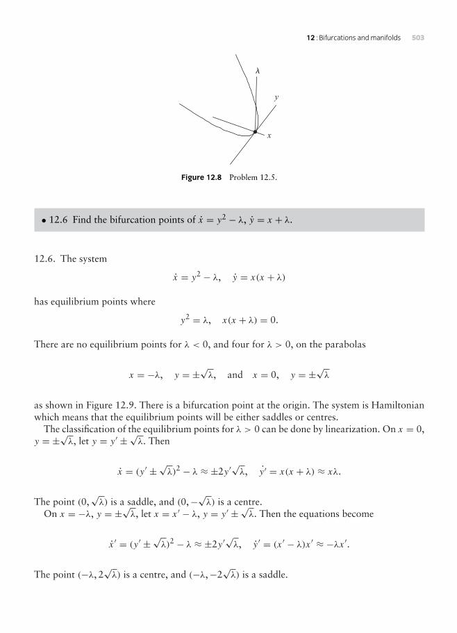
12 : Bifurcations and manifolds 503
x
y
l
Figure 12.8 Problem 12.5.
• 12.6 Find the bifurcation points of x = y2 − λ, y = x + λ.
12.6. The system
x = y2 − λ, y = x(x + λ)
has equilibrium points where
y2 = λ, x(x + λ) = 0.
There are no equilibrium points for λ < 0, and four for λ > 0, on the parabolas
x = −λ, y = ±√λ, and x = 0, y = ±√λ
as shown in Figure 12.9. There is a bifurcation point at the origin. The system is Hamiltonianwhich means that the equilibrium points will be either saddles or centres.
The classification of the equilibrium points for λ > 0 can be done by linearization. On x = 0,y = ±√λ, let y = y′ ± √λ. Then
x = (y′ ± √λ)2 − λ ≈ ±2y′√λ, y′ = x(x + λ) ≈ xλ.
The point (0,√λ) is a saddle, and (0,−√λ) is a centre.
On x = −λ, y = ±√λ, let x = x′ − λ, y = y′ ± √λ. Then the equations become
x′ = (y′ ± √λ)2 − λ ≈ ±2y′√λ, y′ = (x′ − λ)x′ ≈ −λx′.
The point (−λ, 2√λ) is a centre, and (−λ,−2
√λ) is a saddle.

504 Nonlinear ordinary differential equations: problems and solutions
x
y
l
Figure 12.9 Problem 12.6: Showing the parabolas x = 0, y2 = λ and x = −λ, y2 = λ.
x
Figure 12.10 Problem 12.7: Equilibrium points of x = y, y = x(λ− x2).
• 12.7 Consider the system x = y, y = x(λ − x2), −∞ < λ < ∞. Investigate the phasediagrams for λ < 0, λ = 0 and λ > 0. Describe the bifurcation of the system as λ increasesthrough zero.
12.7. The system
x = y, y = x(λ− x2),
has equilibrium points:
(i) at (0, 0), (√λ, 0), (−√λ, 0) if λ > 0;
(ii) at (0, 0) if λ ≤ 0.
There is a bifurcation point at λ = 0. The bifurcation is shown in Figure 12.10 in the (λ, x) ofthe section y = 0. This is a pitchfork bifurcation. The equilibrium point at x = 0 is a centrefor λ < 0, and a saddle for λ > 0. The equilibrium points at x = ±√λ (λ > 0) are centres.

12 : Bifurcations and manifolds 505
x
y
Figure 12.11 Problem 12.8: Pitchfork bifurcation of the system x = y(y2 − λ), y = x + λ.
• 12.8 Discuss the bifurcations of x = (y2 − λ)y, y = x + λ.
12.8. The systemx = y(y2 − λ), y = x + λ
is in equilibrium ify(y2 − λ) = 0, x + λ = 0.
In (x, y, λ) equilibrium occurs on the parabola x = −λ, y = ±√λ, and on the line x = −λ,y = 0 as shown in Figure 12.11. The system is Hamiltonian which implies that the equilibriumpoints are either centres or saddle points.
For λ < 0, let x = −λ+ x′. Then the approximate equations are
x′ ≈ −λy, y′ = x′.
The linear equations predict a centre. For λ > 0, x = −λ, y = 0 is a saddle, and x = −λ,y = ±√λ are centres.
• 12.9 Investigate the bifurcation of the system x = x, y = y2 − λ at λ = 0. Show that, forλ > 0, the system has an unstable node at (0,
√λ) and a saddle point at (0,−√λ). Sketch
the phase diagrams for λ < 0, λ = 0 and λ > 0.
12.9. The systemx = x, y = y2 − λ
has two equilibrium points at x = 0, y = ±√λ if λ > 0, and none if λ < 0, as shown inFigure 12.12. Let y = ±√λ+ y′. Then the equations become
x = x, y′ = (y′ ± √λ)2 − λ ≈ ±2√λy′.
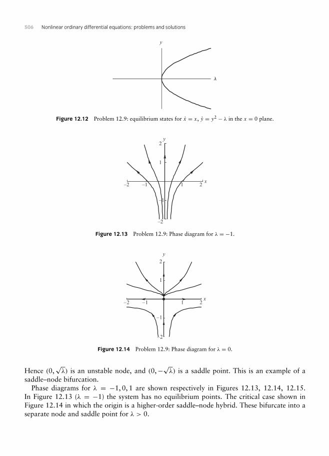
506 Nonlinear ordinary differential equations: problems and solutions
l
y
Figure 12.12 Problem 12.9: equilibrium states for x = x, y = y2 − λ in the x = 0 plane.
–2 –1 1 2x
1
2y
–2
–1
Figure 12.13 Problem 12.9: Phase diagram for λ = −1.
–2 –1 1 2x
–2
–1
1
2
y
Figure 12.14 Problem 12.9: Phase diagram for λ = 0.
Hence (0,√λ) is an unstable node, and (0,−√λ) is a saddle point. This is an example of a
saddle–node bifurcation.Phase diagrams for λ = −1, 0, 1 are shown respectively in Figures 12.13, 12.14, 12.15.
In Figure 12.13 (λ = −1) the system has no equilibrium points. The critical case shown inFigure 12.14 in which the origin is a higher-order saddle–node hybrid. These bifurcate into aseparate node and saddle point for λ > 0.

12 : Bifurcations and manifolds 507
–2 –1 1 2x
–2
–1
2
y
1
Figure 12.15 Problem 12.9: Phase diagram for λ = 1.
Note that the differential equation for the phase paths is
dydx= (y2 − λ)
x,
which is separable, so that the equations for the phase paths can be found explicitly.
• 12.10 A homoclinic path (NODE, Section 3.6) is a phase path which joins an equilibriumpoint to itself in an autonomous system. Show that x = y, y = x − x2 has such a path andfind its equation. Sketch the phase paths for the perturbed system x = y+λx, y = x−x2, forboth λ > 0 and λ < 0. (The homoclinic saddle connection is destroyed by the perturbation;the system undergoes what is known as a homoclinic bifurcation (Section 3.6) at λ = 0.)
12.10. The system
x = y, y = x − x2
has two equilibrium points at (0, 0) (a saddle point) and at (1, 0) (a centre). The phase pathsare given by
dydx= x − x2
y,
which can be integrated to give
12y
2 = 12x
2 − 13x
3 + C.
The homoclinic path passes through the saddle at the origin so that C = 0 leaving the equation
y2 = x2 − 23x
3, (x ≥ 0).

508 Nonlinear ordinary differential equations: problems and solutions
–1 1 2x
–1
1y
Figure 12.16 Problem 12.10: Phase paths for x = y, y = x − x2.
–1 1 2x
–1
1y
Figure 12.17 Problem 12.10: Phase diagram with λ = −0.1.
The phase diagram is shown in Figure 12.16. For the perturbed system
x = y + λx, y = x − x2,
(0, 0) and (1,−λ) are equilibrium points. The origin remains a saddle point. For the other point,let x = 1+ ξ , y = −λ+ η. Then the linearized equations are
ξ = λξ + η, η = (ξ + 1)− (ξ + 1)2 ≈ −ξ .
The classification is as follows:
• λ ≤ −2, stable node;• −2 < λ < 0, stable spiral;• 0 < λ < 2, unstable spiral;• 2 ≤ λ, unstable node.
Phase diagrams for λ = −0.1 and for λ = 0.1 are shown in Figures 12.17 and 12.18.
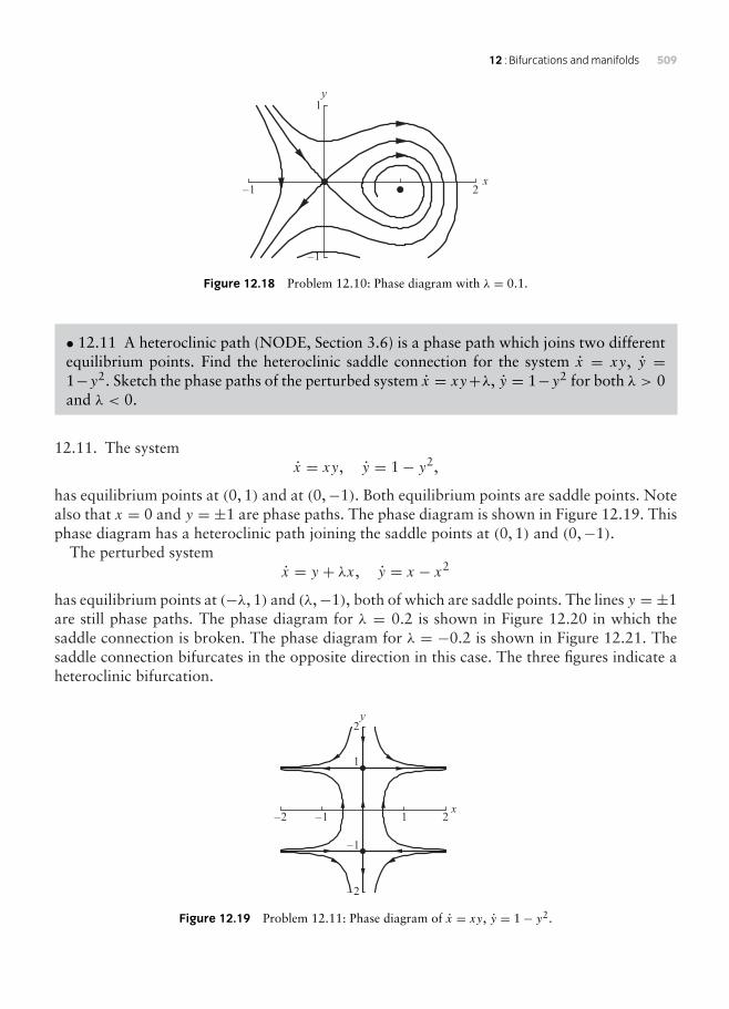
12 : Bifurcations and manifolds 509
–1 2x
–1
1y
Figure 12.18 Problem 12.10: Phase diagram with λ = 0.1.
• 12.11 A heteroclinic path (NODE, Section 3.6) is a phase path which joins two differentequilibrium points. Find the heteroclinic saddle connection for the system x = xy, y =1−y2. Sketch the phase paths of the perturbed system x = xy+λ, y = 1−y2 for both λ > 0and λ < 0.
12.11. The systemx = xy, y = 1− y2,
has equilibrium points at (0, 1) and at (0,−1). Both equilibrium points are saddle points. Notealso that x = 0 and y = ±1 are phase paths. The phase diagram is shown in Figure 12.19. Thisphase diagram has a heteroclinic path joining the saddle points at (0, 1) and (0,−1).
The perturbed systemx = y + λx, y = x − x2
has equilibrium points at (−λ, 1) and (λ,−1), both of which are saddle points. The lines y = ±1are still phase paths. The phase diagram for λ = 0.2 is shown in Figure 12.20 in which thesaddle connection is broken. The phase diagram for λ = −0.2 is shown in Figure 12.21. Thesaddle connection bifurcates in the opposite direction in this case. The three figures indicate aheteroclinic bifurcation.
–2 –1 1 2x
–2
2y
–1
1
Figure 12.19 Problem 12.11: Phase diagram of x = xy, y = 1− y2.

510 Nonlinear ordinary differential equations: problems and solutions
–2 –1 1 2x
–2
–1
1
2y
Figure 12.20 Problem 12.11: Phase diagram for λ = 0.2 .
–2 –1 1 2x
–2
2y
–1
1
Figure 12.21 Problem 12.11: phase diagram for λ = −0.2.
• 12.12 Let
x = −µx − y + x
1+ x2 + y2 , y = x − µy + y
1+ x2 + y2 .
Show that the equations display a Hopf bifurcation as µ > 0 decreases through µ = 1. Findthe radius of the periodic path for 0 < µ < 1.
12.12. Express the system
x = −µx − y + x
1+ x2 + y2 , y = x − µy + y
1+ x2 + y2
in polar coordinates with x = r cos θ , y = r sin θ . Then
rr = xx + yy = −µr2 + r2
1+ r2 = −r2
1+ r2 [µr2 + (µ− 1)],
θ = 1r2 (yx − xy) = 1.

12 : Bifurcations and manifolds 511
For 0 < µ < 1, r = r0 = √[(1− µ)/µ] is a limit cycle which is stable since for r < r0, r > 0,and for r > r0, r < 0. In other words adjacent paths spiral into the limit cycle. The equilibriumpoint at the origin is an unstable spiral.
For µ > 1, the system has a stable equilibrium point at the origin and no limit cycle. Thesystem passes through a Hopf bifurcation as µ decreases through µ = 1.
• 12.13 Show that the system
x = x − γ y − x(x2 + y2), y = γ x + y − y(x2 + y2)− γ , (γ > 0)
has a bifurcation point at γ = 12 , by investigating the numbers of equilibrium points for
γ > 0. Compute the phase diagram for γ = 14
12.13. The system
x = x − γ y − x(x2 + y2), y = γ x + y − y(x2 + y2)− γ , (γ > 0)
has equilibrium points where
x − γ y − x(x2 + y2) = 0, γ x + y − y(x2 + y2) = γ (i)
Squaring and adding
[x − γ y − x(x2 + y2)]2 + [γ x + y − y(x2 + y2)]2 = γ 2,
orr2(1− r2)2 − γ 2(1− r2) = 0,
where r2 = x2 + y2. Therefore
r = 1, or r4 − r2 + γ 2 = 0. (ii)
The cases are as follows:
• γ > 12 . Equation (ii) has one real solution where r = 1, which from (i) implies that (1, 0)
is an equilibrium point. To classify the point, let x = 1+ ξ . Then
ξ ≈ −2ξ − γ y, y ≈ γ ξ .
Therefore (1, 0) is a stable node for 12 < γ < 1.
• γ = 12 . In this case (ii) has the solutions r = 1 and r = 1/
√2 which lead to equilib-
rium points at (1, 0) and at (12 , 1
2 ). As in the previous case (1, 0) remains a stable node.

512 Nonlinear ordinary differential equations: problems and solutions
–1 1x
–1
1
y
P Q
Figure 12.22 Problem 12.13.
Linearization is not helpful for (12 , 1
2 ) since the equations for the perturbations ξ and ηbecome
ξ ≈ −η, η ≈ 0,
which is a degenerate case.
• 0 < γ < 12 . (ii) now has three real solutions r = 1, and r = r1, r2 = 1
2 (1±√(1− 4γ 2)). The
origin remains a stable node. Classification of the other equilibrium points is complicated.
As the parameter γ decreases through γ = 12 an equilibrium point appears at (1
2 , 12 ) which then
splits into two equilibrium points. The phase diagram for γ = 0.25 is shown in Figure 12.22.The computed diagram seems to indicate that the bifurcation creates an unstable node at P ,and a saddle point at Q. The equilibrium point at (1, 0) is a stable node for γ < 1.
• 12.14 Let x = Ax, where x = [x y z]T . Find the eigenvalues and eigenvectors of A ineach of the following cases. Describe the stable and unstable manifolds of the origin.
(a) A = 1 1 2
1 2 12 1 1
.
(b) A = 3 0 −1
0 1 02 0 0
.
(c) A = 2 0 0
0 2 20 2 −1
.
(d) A = 6 5 5
5 6 55 5 6
.

12 : Bifurcations and manifolds 513
12.14. The origin is an equilibrium point for the linear system
x = Ax.
(a)
A = 1 1 2
1 2 12 1 1
.
The eigenvalues of A are given by
∣∣∣∣∣∣1− λ 1 2
1 2− λ 12 1 1− λ
∣∣∣∣∣∣ = 0, or − (λ− 4)(λ− 1)(λ+ 1) = 0.
Therefore the eigenvalues are −1, 1, 4 with corresponding eigenvectors
(−1, 0, 1)T , (1,−2, 1)T , (1, 1, 1)T .
Hence the general solution is given by
x
y
z
= α
−1
01
e−t + β
1−21
et + γ
1
11
e4t .
The stable manifold is given parametrically by β = γ = 0, that is
x
y
z
= α
−1
01
e−t ,
which is the straight line z = −x, y = 0.The unstable manifold is given by
x
y
z
= β
1−21
et + γ
1
11
e4t ,
which defines the plane x − 3z = 0.
(b)
A = 3 0 −1
0 1 02 0 0
.

514 Nonlinear ordinary differential equations: problems and solutions
The eigenvalues of A are given by
∣∣∣∣∣∣3− λ 0 −1
0 1− λ 02 0 −λ
∣∣∣∣∣∣ = 0, or − (λ− 2)(λ− 1)2 = 0.
Therefore the eigenvalues are 1(repeated) and 2 with corresponding eigenvectors
(1, 0, 2)T , (0, 1, 0)T , (1, 0, 1)T .
Hence the general solution
x
y
z
= α
1
02
et + β
0
10
et + γ
1
01
e2t .
Since all the eigenvalues are positive there is no stable manifold, and the unstable manifold isthe whole space.
(c)
A = 2 0 0
0 2 20 2 −1
.
The eigenvalues of A are given by
∣∣∣∣∣∣2− λ 0 0
0 2− λ 20 2 −1− λ
∣∣∣∣∣∣ = 0, or − (λ− 3)(λ− 2)(λ+ 2) = 0.
Therefore the eigenvalues are −2, 2, 3 with corresponding eigenvectors
(0,−1, 2)T , (1, 0, 0)T , (0, 2, 1)T .
Hence the general solution is
x
y
z
= α
0−12
e−2t + β
1
00
e2t + γ
0
21
e3t .
The stable manifold (β = γ = 0, α = 1, say) is the straight line given parametrically by x = 0,y = −e−2t , z = 2e−2t . The unstable manifold (α = 0) is the plane −y + 2z = 0.
(d)
A = 6 5 5
5 6 55 5 6
.

12 : Bifurcations and manifolds 515
The eigenvalues of A are given by
∣∣∣∣∣∣6− λ 5 5
5 6− λ 55 5 6− λ
∣∣∣∣∣∣ = 0, or − (λ− 16)(λ− 1)2 = 0.
Therefore the eigenvalues are 1(repeated) and 16 with corresponding eigenvectors
(−1, 0, 1)T , (−1, 1, 0)T , (1, 1, 1)T .
Hence the general solution is
x
y
z
= α
−1
01
et + β
−1
10
et + γ
1
11
e16t .
Since the eigenvalues are all positive there is no stable manifold, whilst the stable manifold isthe whole space.
• 12.15 Show that x = Ax where x = [x y z]T and
A = −3 0 −2−4 −1 −43 1 3
has two imaginary eigenvalues. Find the equation of the centre manifold of the origin. Isthe remaining manifold stable or unstable?
12.15. In the system x = Ax,
A = −3 0 −2−4 −1 −43 1 3
.
The eigenvalues of A are given by
∣∣∣∣∣∣−3−m 0 −2−4 −1−m −43 1 3−m
∣∣∣∣∣∣ = −(m+ 1)(m2 + 1) = 0.
The eigenvalues are −1,−i, i with corresponding eigenvectors
[−1,−1, 1]T , [−3− i,−6− 2i, 5]T , [−3+ i,−6+ 2i, 5]T .

516 Nonlinear ordinary differential equations: problems and solutions
Therefore the general solution is
x
y
z
= α
−1−11
e−t + β
−3− i−6− 2i
5
e−it + β
−3+ i−6+ 2i
5
eit ,
where α is a real constant and β is a complex constant.The system has a stable manifold which is the line given parametrically (put β = 0 and
α = 1) by (x, y, z) = (−e−t ,−e−t , et ). Since the other eigenvalues are imaginary, the origin hasan associated centre manifold defined by α = 0, namely by
x
y
z
= β
−3− i−6− 2i
5
e−it + β
−3+ i−6+ 2i
5
eit ,
which defines the plane −2x + y = 0. Depending on the initial values, as t → ∞, solutionsapproach a periodic solution of the centre which lies in the plane −2x + y = 0.
• 12.16 Show that the centre manifold of x
y
z
=
−1 0 1
0 1 −20 1 −1
=
x
y
z
,
is given by 2x + y − 2z = 0
12.16. Let
A = −1 0 1
0 1 −20 1 −1
.
The eigenvalues of A are given by
∣∣∣∣∣∣−1−m 0 1
0 1−m −20 1 −1−m
∣∣∣∣∣∣ = −(m+ 1)(m2 + 1) = 0.
The eigenvalues are −1,−i, i with corresponding eigenvectors
[1, 0, 0]T , [1+ i, 2− 2i, 2]T , [1− i, 2+ 2i, 2]T .

12 : Bifurcations and manifolds 517
Therefore the general solution is
x
y
z
= α
1
00
e−t + β
1+ i
2− 2i2
e−it + β
1− i
2+ 2i2
eit ,
where α is a real constant and β is a complex constant. Solutions for which α = 0 lie on thecentre manifold, that is,
x
y
z
= β
1+ i
2− 2i2
e−it + β
1− i
2+ 2i2
eit ,
which is the plane −2x − y + 2z = 0.
• 12.17 Show that the phase paths of x = y(x + 1), y = x(1− y2) are given by
y = ±√[1− Ae−2x(1+ x)2],with singular solutions x = −1 and y = ±1. Describe the domains in the (x, y) plane of thestable and unstable manifolds of each of the three equilibrium points of the system.
12.17. The phase paths of
x = y(x + 1), y = x(1− y2),
are given bydydx= x(1− y2)
y(x + 1).
Separating the variables and integrating,
∫ydy
1− y2 =∫
xdxx + 1
+ B.
Therefore
−12 ln |1− y2| = − ln[e−x |x + 1|] + B,
or
y = ±√[1− Ae−2x(1+ x)2].By inspection the equations also have the solutions x = −1 and y = ±1.
The system has equilibrium points at (0, 0), (−1, 1) and (−1,−1). The classification ofthe equilibrium points is as follows (easier to use the differential equations rather than thesolutions):• (0, 0): x ≈ y, y ≈ x – saddle point;

518 Nonlinear ordinary differential equations: problems and solutions
1x
y
A
B
C
D
E
F
G
–1
–1
1
Figure 12.23 Problem 12.17: Phase diagram for x = y(x + 1), y = x(1− y2).
• (−1, 1): let x = −1+ x′, y = 1+ y′; then x′ ≈ x′, y′ ≈ 2y′ – unstable node;• (−1,−1); let x′ = 1+ x′, y = −1+ y′; then x′ ≈ −x′, y′ ≈ −2y′– stable node.
For the saddle point at the origin, the stable manifolds are the separatrices EA and BA inFigure 12.23.
For the equilibrium point at (−1, 1), the domain above GCAD is its unstable manifold.For the equilibrium point at (−1,−1), the domain below FBAE is its stable manifold.
• 12.18 Show that the linear approximation at (0, 0, 0) of
x = −y+yz+(y−x)(x2+y2), y = x−xz−(x+y)(x2+y2), z = −z+(1−2z)(x2+y2),
has a centre manifold there. Show that z = x2+y2 is a solution of this system of equations.To which manifold of the origin is this surface tangential? Show also that, on the surface,x and y satisfy
x = −y + (2y − x)(x2 + y2), y = x − (2x + y)(x2 + y2).
Using polar coordinates determine the stability of solutions on this surface and the stabilityof the origin.
12.18. The linear approximation near (0, 0, 0) of the system
x = −y + yz+ (y − x)(x2 + y2), y = x − xz− (x + y)(x2 + y2),
z = −z+ (1− 2z)(x2 + y2),
is
x ≈ −y, y ≈ x, z ≈ −z.
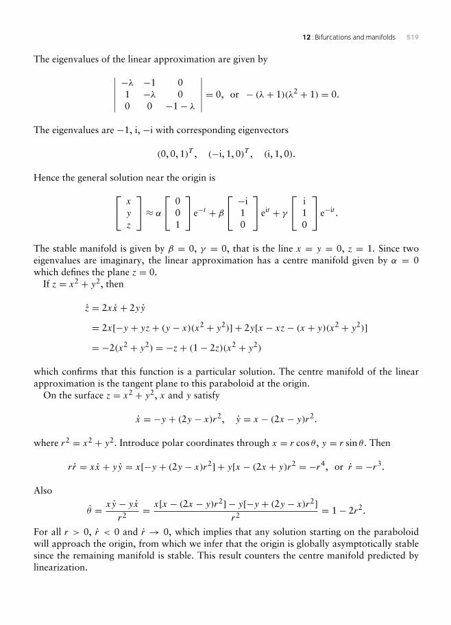
12 : Bifurcations and manifolds 519
The eigenvalues of the linear approximation are given by
∣∣∣∣∣∣−λ −1 01 −λ 00 0 −1− λ
∣∣∣∣∣∣ = 0, or − (λ+ 1)(λ2 + 1) = 0.
The eigenvalues are −1, i, −i with corresponding eigenvectors
(0, 0, 1)T , (−i, 1, 0)T , (i, 1, 0).
Hence the general solution near the origin is
x
y
z
≈ α
0
01
e−t + β
−i
10
eit + γ
i
10
e−it .
The stable manifold is given by β = 0, γ = 0, that is the line x = y = 0, z = 1. Since twoeigenvalues are imaginary, the linear approximation has a centre manifold given by α = 0which defines the plane z = 0.
If z = x2 + y2, then
z = 2xx + 2yy
= 2x[−y + yz+ (y − x)(x2 + y2)] + 2y[x − xz− (x + y)(x2 + y2)]= −2(x2 + y2) = −z+ (1− 2z)(x2 + y2)
which confirms that this function is a particular solution. The centre manifold of the linearapproximation is the tangent plane to this paraboloid at the origin.
On the surface z = x2 + y2, x and y satisfy
x = −y + (2y − x)r2, y = x − (2x − y)r2.
where r2 = x2 + y2. Introduce polar coordinates through x = r cos θ , y = r sin θ . Then
rr = xx + yy = x[−y + (2y − x)r2] + y[x − (2x + y)r2 = −r4, or r = −r3.
Also
θ = xy − yxr2 = x[x − (2x − y)r2] − y[−y + (2y − x)r2]
r2 = 1− 2r2.
For all r > 0, r < 0 and r → 0, which implies that any solution starting on the paraboloidwill approach the origin, from which we infer that the origin is globally asymptotically stablesince the remaining manifold is stable. This result counters the centre manifold predicted bylinearization.

520 Nonlinear ordinary differential equations: problems and solutions
m
x
Stable
Unstable
Figure 12.24 Problem 12.19: Stability diagram for x = µx − x2, y = y(µ− 2x).
• 12.19 Investigate the stability of the equilibrium points of x = µx − x2, y = y(µ − 2x)in terms of the parameter µ. Draw a stability diagram in the (µ, x) plane for y = 0. Whattype of bifcurcation occurs at µ = 0? Obtain the equations of the phase paths, and sketchthe phase diagrams in the cases µ = −1, µ = 0 and µ = 1.
12.19. The systemx = µx − x2, y = y(µ− 2x)
has equilibrium points at (0, 0) and (µ, 0). The linear classification of the points is as follows.
• (0, 0). The linear approximation is
x ≈ µx, y ≈ µy,
which is a critical node, stable if µ < 0 and unstable if µ > 0.• (µ, 0). Let x = µ+ ξ . Then
ξ ≈ −µξ , y ≈ −µy,
which is also a critical node, stable if µ > 0 and unstable if µ < 0.
The stability diagram of equilibrium points in the (µ, x) plane is shown in Figure 12.24. Theorigin is an example of a transcritical bifurcation.
The phase paths are given by solutions of
dydx= y(µ− x)x(µ− x) .
Separation of variables leads to
∫dyy=
∫µ− 2xx(µ− x)dx,

12 : Bifurcations and manifolds 521
–2 –1 1x
–1
1y
–1 1x
–1
1y
Figure 12.25 Problem 12.19: Phase diagrams for, respectively µ = −1 and µ = 0.
–1 1 2x
–1
1y
Figure 12.26 Problem 12.19: phase diagram for µ = 1.
orln |y| = ln |x(x − µ)| + C, or y = Bx(x − µ).
The straight lines x = 0, x = µ and y = 0 are also phase paths. The phase diagrams for µ = −1and µ = 0 are shown in Figure 12.25. The phase diagram for µ = 1 is shown in Figure 12.26.
• 12.20 Where is the bifurcation point of the parameter-dependent system
x = x2 + y2 − µ, y = 2µ− 5xy?
Discuss how the system changes as µ increases. For µ = 5, find all linear approximationsfor all equilibrium points and classify them.
12.20. The systemx = x2 + y2 − µ, y = 2µ− 5xy,
is in equilibrium wherex2 + y2 − µ = 0, 2µ− 5xy = 0.
Elimination of y leads to
25x4 − 25µx2 + 4µ2 = 0, or (5x2 − 4µ)(5x2 − µ) = 0.

522 Nonlinear ordinary differential equations: problems and solutions
where y = 2µ/(5x). If µ < 0, the system has no equilibrium points, if µ = 0 the system hasone point, at (0, 0), and if µ > 0, the system has four points, at
(2√µ√5
,√µ√5
),
(−2√µ√
5,−√µ√
5
),
(√µ√5
,2√µ√5
),
(−√µ√5
,−2√µ√
5
).
The system has a bifurcation point at µ = 0. As µ increases through zero, a single equilibriumpoint emerges at the origin at µ = 0 which splits into four equilibrium points as µ becomespositive.
If µ = 5, the equilibrium points simplify to the coordinates (2, 1), (−2,−1), (1, 2), (−1,−2).The linear classification is as follows:
• (2, 1). Let x = 2+ ξ , y = 1+ η. Then
ξ = (2+ ξ)2 + (1+ η)2 − 5 ≈ 4ξ + 2η,
η = 10− 5(2+ ξ)(1+ η) ≈ −5ξ − 10η.
In the usual notation p = −6 < 0, q = −30 < 0, which implies that (2, 1) is a saddle.
• (−2,−1). Let x = −2+ ξ , y = −1+ η. Then
ξ = (−2+ ξ)2 + (−1+ η)2 − 5 ≈ −4ξ − 2η,
η = 10− 5(−2+ ξ)(−1+ η) ≈ 5ξ + 10η.
Therefore p = 6 > 0, q = −30 < 0, which implies that (−2,−1) is a saddle.
• (1, 2). Let x = 1+ ξ , y = 2+ η. Then
ξ = (1+ ξ)2 + (2+ η)2 − 5 ≈ 2ξ + 4η,
η = 10− 5(1+ ξ)(2+ η) ≈ −10ξ − 5η.
Therefore p = −3 < 0, q = 30 > 0, = −111 < 0, which implies that (1, 2) is a stablespiral.
• (−1,−2). Let x = −1+ ξ , y = −2+ η. Then
ξ = (−1+ ξ)2 + (−2+ η)2 − 5 ≈ −2ξ − 4η,
η = 10− 5(−1+ ξ)(−2+ η) ≈ 10ξ + 5η.
Therefore p = 3 > 0, q = 30, = −111, which implies that (−1,−2) is an unstablespiral.

12 : Bifurcations and manifolds 523
r
f (r)
A B
m > 0
Figure 12.27 Problem 12.21:
• 12.21 Obtain the polar equations for (r, θ) of
x = y + x[µ− (x2 + y2 − 1)2], y = −x + y[µ− (x2 + y2 − 1)2],where |µ| < 1. Show that, for 0 < µ < 1, the system has two limit cycles, one stable andone unstable, which collide at µ = 0 and disappear for µ < 0. This is an example of a bluesky catastrophe in which a finite amplitude limit cycles simply disappears as a parameter ischanged incrementally.
12.21. In the system
x = y + x[µ− (x2 + y2 − 1)2], y = −x + y[µ− (x2 + y2 − 1)2],
let x = r cos θ , y = r sin θ . In terms of r and θ the equations become
r = xx + yy = r[µ− (r2 − 1)2] = f (r) say,
θ = yx − xyr2 = −1.
For µ > 0, the general shape of f (r) versus r is shown in Figure 12.27. The zero at r = 0 isan equilibrium point, whilst the zeros at A and B define limit cycles of the system. For point A,r = √(1−√µ) and for B, r = √(1+√µ). As µ decreases through zero the two limit cyclesmerge at r = 1 and then disappear for µ < 0.
• 12.22 Discuss the bifurcations of the equilibrium points of x = y, y = −x − 2x2 − µx3
for −∞ < µ < ∞. Sketch the bifurcation diagram in the (µ, x) plane. Confirm that thereis a bifurcation at µ = 1. What happens at µ = 0?
12.22. Equilibrium ofx = y, y = −x − 2x2 − µx3,

524 Nonlinear ordinary differential equations: problems and solutions
–1 1 2
–8
–4
4
8x
A
O m
Figure 12.28 Problem 12.22.
occurs where y = 0 and µx3 + 2x2 + x = 0. The solutions of the latter equation are
x = 0, x = 1µ[−1±√(1− µ)], (µ = 0, µ < 1).
If µ = 0, the system has two equilibrium points, at x = 0 and x = −12 . If µ > 1, then the
system has one equilibrium point, at x = 0As µ decreases through µ = 1, two additional equilibrium points appear at µ = 1 (point A
in Figure 12.28). One of these disappears as µ → 0 (point O), and x → −∞, but a secondpoint re-appears immediately for large positive x.
• 12.23 Consider the system x = y − x(x2 + y2 − µ), y = −x − y(x2 + y2 − µ), where µis a parameter. Express the equations in polar form in terms of (r, θ) show that the originis a stable spiral for µ < 0, and unstable spiral for µ > 0. What type of bifurcation occursat µ = 0?
12.23. The system
x = y − x(x2 + y2 − µ), y = −x − y(x2 + y2 − µ)
has one equilibrium point, at (0, 0). Let x = r cos θ and y = r sin θ , so that the polar equationsare
r = −r(r2 − µ), θ = −1.
This system has a stable limit cycle at r = √µ if µ > 0. If µ < 0 the origin is a global stablespiral. A stable limit cycle appears from the origin as µ increases through zero. This is a Hopfbifurcation.

12 : Bifurcations and manifolds 525
–2 –1 1 2x
–2
–1
1
2y
Figure 12.29 Problem 12.24: Phase diagram with µ = 2.3 showing stable and unstable limit cycles.
• 12.24 In polar form a system is given by r = r(r2 − µr + 1), θ = −1, where µ is aparameter. Discuss the bifurcations which occur as µ increases through µ = 2.
12.24. The polar equations of a system are given by
r = r(r2 − µr + 1), θ = −1.
Equilibrium occurs where r = 0. r = 0 where
r = 12 [µ±
√(µ2 − 4)]. (i)
If µ < −2, then r < 0. If µ > 2 then the system has two limit cycles with radii given by (i). Inthis case the origin is an unstable spiral, and the inner limit cycle is stable and the outer oneunstable as shown in Figure 12.29. As µ increases through µ = 2 a limit cycle appears whichimmediately bifurcates into two limit cycles.
• 12.25 The equations of a displaced van der Pol oscillator are given by
x = y − a, y = −x + δ(1− x2)y,
where a > 0 and δ > 0. If the parameter a = 0 then the usual equations for the vander Pol oscillator appear. Suppose that a is increased from zero. Show that the system hastwo equilibrium points one of which is a saddle point at x ≈ −1/(aδ), y = a for small a.Compute phase paths for δ = 2, and a = 0, 1, 0.2, 0.4, and observe that the saddle pointapproaches with the limit cycle of the van der Pol equation. Show that at a ≈ 0.31 thesaddle point collides with the limit cycle, which then disappears.

526 Nonlinear ordinary differential equations: problems and solutions
12.25. The displaced van der Pol equations are
x = y − a, y = −x + δ(1− x2)y, (a > 0, δ > 0).
Equilibrium occurs where
y = a, x − δ(1− x2)a = 0.,
that is, where
x = x1, x2 = 12δa
[−1±√(1+ 4δ2a2)].
Therefore there are two equilibrium points at (x1, a) and (x2, a). The linear classifications atthese points are as follows.
• (x1, a). Let x = x1 + ξ and y = a + η. Then ξ = η, and
η = −(x1 + ξ)+ δ[1− (x1 + ξ)2](a + η)≈ (−1− 2x1aδ)ξ + δ(1− x2
1)η
In the usual notation
p = δ(1− x21) =
x1
a= 1
2δa2 [−1+√(1+ 4δ2a2)] > 0,
q = 1+ 2aδx1 = √(1+ 4δ2a2) > 0,
which implies that (x1, a) is an unstable node or spiral.• (x2, a). Let x = x2 + ξ and y = a + η. Then ξ = η, and
η = −(x2 + ξ)+ δ[1− (x2 + ξ)2](a + η)≈ (−1− 2x2aδ)ξ + δ(1− x2
2)η
In this case
p = δ(1− x22) =
x2
a= 1
2δa2 [−1−√(1+ 4δ2a2)] < 0,
q = 1+ 2aδx1 = −√(1+ 4δ2a2), 0,
which implies that (x2, a) is a saddle.
As a increases from zero, the saddle point B approaches from infinity and collides with the limitcycle as shown in the sequence of Figures 12.30, 12.31, 12.32. At a = 0 the limit cycle is vander Pol cycle, which becomes distorted by the approaching saddle, and eventually disappearsat a ≈ 0.31.

12 : Bifurcations and manifolds 527
–6 –4 –2 2x
–4
–2
4y
AB
2
Figure 12.30 Problem 12.25: For δ = 2, a = 0.1, the saddle is at B and the unstable spiral at A.
–6 –4x
–4
–2
4y
AB
–2 2
2
Figure 12.31 Problem 12.25: For δ = 2, a = 0.2, the saddle is at B and the unstable spiral at A.
–6 –4 2x
–4
–2
2
4
y
AB
–2–2
Figure 12.32 Problem 12.25: For δ = 2, a = 0.4, the saddle is at B and the unstable spiral at A; the limit cycle hasnow disappeared.

528 Nonlinear ordinary differential equations: problems and solutions
• 12.26 Find the stable and unstable manifolds of the equilibrium points of
x = x2 + µ, y = −y, z = z,for µ < 0. What type of bifurcation occurs at µ = 0?
12.26. The equilibrium points of the system
x = x2 + µ, y = −y, z = z
occur at (±√(−µ), 0, 0). The solutions are
x = √(−µ) tanh[−√(−µ)t + A], y = Be−t , z = Cet .
For x with A = 0, as t →∞, x →−√(−µ), and as t →−∞, x →√(−µ).
• For (√(−µ), 0, 0), the stable manifold is the straight line x = √(−µ), z = 0. The unstable
manifold is the half-plane y = 0, x > −√(−µ).• For (−√(−µ), 0, 0), the unstable manifold is the straight line x = √
(−µ), y = 0. Thestable manifold is the half-plane y = 0, x <
√(−µ).
• 12.27 Consider the system x = µx − y − x3, y = x + µy − y3. By putting z = µ − x2,show that any equilibrium points away from the origin are given by the solutions of z4 −µz3+µz+1 = 0. Plot the graph of µ against z and show that there is only one equilibriumpoint at the origin if µ < 2
√2, approximately, and nine equilibrium points if µ > 2
√2
Investigate the linear approximation for the equilibrium point at the origin and show thatthe system has a Hopf bifurcation there at µ = 0. Compute the phase diagram for µ = 1.5.
12.27. The equilibrium points of
x = µx − y − x3, y = x + µy − y3,
satisfyµx − y − x3 = 0, x + µy − y3 = 0.
Eliminate y so that
x + µ(µx − x3)− (µx − x3)3 = 0, or x[1+ µ(µ− x2)− x2(µ− x2)3] = 0.
One solution is x = 0. For the others express the remaining equation in the form
1+ µ(µ− x2)+ (µ− x2)4 − µ(µ− x2)3 = 0.

12 : Bifurcations and manifolds 529
–6 –4 –2 2 4 6z
–8
–6
–4
–2
2
4
6
8
m = z
m
Figure 12.33 Problem 12.27: Graph of µ = (z4 + 1)/(z(z2 − 1)); only solutions above the dashed line µ = z are ofinterest.
Let z = µ− x2, so that z satisfies
z4 − µz3 + µz+ 1 = 0.
Therefore
µ = z4 + 1z(z2 − 1)
= f (z),
say. Real solutions for x can only occur if µ > z. The graph of µ against z is shown inFigure 12.33. Stationary values of µ = f (z) occur where f ′(z) = 0, namely where
z6 − 3z4 − 3z2 + 1 = (1+ z2)(1− 4z2 + z4) = 0.
Real solutions can only occur if z4 − 4z2 + 1 = 0, that is where
z2 = 2±√3.
To satisfy µ > z we must choose z = √[2+√3] and z = −√[2−√3]. Both values of z givethe same value for µ, namely µ = 2
√2. Therefore there is one equilibrium point if µ < 2
√2,
5 equilibrium points if µ = 2√
2, and 9 if µ > 2√
2.Near the origin
x ≈ µx − y, y ≈ x + µy.
In the usual notation
p = 2µ, q = µ2 + 1 > 0, = p2 − 4q = −4 < 0.
As µ increases through zero a stable spiral becomes an unstable spiral. Switch to polarcoordinates. Then
rr = xx + yy = µr2 − (x4 + y4).

530 Nonlinear ordinary differential equations: problems and solutions
–2 2x
–2
2
y
Figure 12.34 Problem 12.27: Limit cycle for x = µx − y − x3, y = x + µy − y3 with µ = 1.5.
With x = r cos θ and y = r sin θ ,
x4 + y4 − µr2 = r4(cos4 θ + sin4 θ)− µr2 ≥ 12r
4 − µr2
= 12r
2(r2 − 2µ) > 0
for r2 > 2µ. It follows that r < 0 for r sufficiently large which means that the radial pathsare decreasing if µ is positive. Therefore there must be at least one stable periodic solutiongenerated at the origin at µ = 0. For µ < 0, r > 0 on all paths. Hence this is an example of aHopf bifurcation. A phase diagram for the system with µ = 1.5 is shown in Figure 12.34. Thelimit cycle has been created by a Hopf bifurcation at µ = 0.
• 12.28 Show that the system x = x2+y+z+1, y = z−xy, z = x−1 has one equilibriumpoint at (1,−1,−1). Determine the linear approximation x′ = Ax′ to the system at thispoint. Find the eigenvalues and eigenvectors of A, and the equations of the stable andunstable manifolds Es and Ec of the linear approximation.
12.28. The systemx = x2 + y + z+ 1, y = z− xy, z = x − 1,
is in equilibrium where
x2 + y + z+ 1 = 0, z = xy, x = 1.
The only solution is x = 1, y = −1, z = −1. Let x = 1 + x′, y = −1 + y′, z = −1 + z′. Thenthe linearized matrix equation is x′ = Ax′, where
A = 2 1 1
1 −1 11 0 0
.

12 : Bifurcations and manifolds 531
The eigenvalues are given by
∣∣∣∣∣∣2− λ 1 1
1 −1− λ 11 0 −λ
∣∣∣∣∣∣ = 0, or − (λ+ 1)(λ2 − 2λ− 2) = 0.
Therefore the eigenvalues are λ1 = −1, λ2 = 1 + √3, λ3 = 1 − √3, and the correspondingeigenvectors are
r1 = [−1, 2, 1]T , r2 = [1−√
3, 1, 1]T , r3 = [1+√
3, 1, 1]T .
The general solution is
x′y′z′
= α
−1
21
e−t + β
1−√3
11
e(1−
√3)t + γ
1+√3
11
e(1+
√3)t .
The stable manifold is given by γ = 0, which is given parametrically by the equations
x′ = −α + (1−√3)β,
y′ = 2α + β,
z′ = α + β.
In terms of x, y, z the stable manifold is the plane
(x − 1)+ (2−√3)(y + 1)+ (2√3− 3)(z+ 1) = 0.
The unstable manifold is defined by α = β = 0, which defines the straight line
x′ = x − 1 = (1+√3)s, y′ = y + 1 = s, z′ = z+ 1 = s.
• 12.29 Consider the equation z = λz− |z|2z, where z = x + iy is a complex variable, andλ = α + iβ is a complex constant. Classify the equilibrium point at the origin, and showthat the system has a Hopf bifurcation as α increases through zero for β = 0. How doesthe system behave if β = 0?
12.29. In the equation z = λz − |z|2z, let z = x + iy and λ = α + iβ. The real and imaginaryequations are
x = αx − βy − (x2 + y2)x,
y = βx + αy − (x2 + y2)y.

532 Nonlinear ordinary differential equations: problems and solutions
The system has one equilibrium point, at (0, 0). Near the origin
x ≈ αx − βy, y ≈ βx + αy.
In the usual notation, the classification parameters are
p = 2α, q = α2 + β2 > 0, = p2 − 4q = −4β2 < 0.
As α increases through zero the origin changes from a stable spiral to an unstable spiral. ByTheorem 12.1, a Hopf bifurcation occurs at µ = 0.
In polar coordinates (r, θ),r = r(α − r2).
If α > 0, the limit cycle is the circle of radius√α.
If β = 0, the equations become
x = (α − r2)x, y = (α − r2)y.
Equilibrium occurs at (0, 0) only if α ≤ 0, and at (0, 0) and all points on the circle r = √α ifα > 0. The phase paths are given by
dydx= y
x,
which has the general solution y = Cx. The phase paths are radial lines through the origin.

13Poincaré sequences,homoclinic bifurcation,and chaos
• 13.1 Obtain the solutions for the usual polar coordinates r and θ in terms of t , for thesystem
x = x + y − x(x2 + y2), y = −x + y − y(x2 + y2).
Let be the section θ = 0, r > 0. Find the difference equation for the Poincaré sequencein this section.
13.1. In the equations
x = x + y − x(x2 + y2), y = −x + y − y(x2 + y2),
let x = r cos θ , y = r sin θ . Then
r = r(1− r2), θ = xy − xyr2 = −1.
Integration of the equations leads to
r = r0√[r20 + (1− r2
0 )e−2t ] , θ = −t + θ0,
where r(0) = r0, θ(0) = θ0. The system has an equilibrium point at the origin, which is anunstable spiral. The system also has a stable limit cycle given by circle r = 1.
The polar equations of the paths are given by
r = r0√[r20 + (1− r2
0 )e2(θ−θ0)] .
In the section , θ0 = 0, and successive returns occur at θ = −2π ,−4π , . . . . Denoting theseradii by rn, we have
rn = r0√[r20 + (1− r2
0 )e−4πn] .
As expected, as n→∞, rn→ 1 irrespective of the initial value r0.

534 Nonlinear ordinary differential equations: problems and solutions
• 13.2 Find the map of 2π first returns on the section : t = 0 for x + 2x + 2x = 2 sin t inthe usual phase plane. Find also the coordinates of the fixed point of the map and discussits stability. Where is the fixed point of the map if the section is t = 1
2π?
13.2. The linear equationx + 2x + 2x = 2 sin t ,
has the general solution
x = (A cos t + B sin t)e−t − 45 cos t + 2
5 sin t . (i)
It follows that
x = [−(A− B) cos t + (A+ B) sin t]e−t + 25 cos t + 4
5 sin t . (ii)
Equations (i) and (ii) give represent points parametrically in the phase plane x, x = y. At t = 0,
x(0) = x0 = A− 45 , y(0) = y0 = −A+ B + 2
5 .
The first return is given by
x(2π) = x1 = Ae−2π − 45 , y(2π) = y1 = (−A+ B)e−2π + 2
5 .
Elimination of A and B leads to
x1 = (x0 + 45 )e
−2π − 45 , y1 = (y0 + A− B)e−2π + 2
5 .
The fixed point of the map occurs where x1 = x0 and y1 = y0 which results in A = B = 0leading to the fixed point (−4
5 , 25 ).
If the section is t = 12π , then from (i) and (ii) again
x(12π) = u0 = Be−(1/2)π + 2
5 , y(12π) = v0 = (A+ B)e−(1/2)π + 4
5 .
The first return is given by
x(52π) = u1 = Be−(5/2)π + 2
5 , y(52π) = v1 = (A+ B)e−(5/2)π + 4
5 .
Then u0 = u1 and v0 = v1 if A = B = 0 which leads to the fixed point (25 , 4
5 ).Alternatively for this linear equation the fixed points can be found by simply eliminating the
exponential terms in the solution by putting A = B = 0. All fixed points for any section canthen be read off.

13 : Poincaré sequences, homoclinic bifurcation, and chaos 535
• 13.3 Let x1 satisfy x1 + 14ω
2x1 = cosωt . Obtain the solutions for x1 and x2 = x1 giventhat x1(0) = x10 and x2(0) = x20. Let be the section t = 0 and find the first returns ofperiod 2π/ω. Show that the mapping is
P(x10, x20) =(−x10 − 8
3ω2 ,−x20
), and that P 2
(x10, x20) = (x10, x20).
Deduce that the system exhibits period doubling for all initial values except one. Find thecoordinates of this fixed point.
13.3. The equationx1 + 1
4ω2x1 = cosωt ,
has the general solution
x1 = A cos 12ωt + B sin 1
2ωt −43ω2 cosωt . (i)
It follows that
x2 = x1 = −12ωA sin 1
2ωt + 12ωB cosωt + 4
3ωsinωt . (ii)
From the given initial conditions
A = x10 + 43ω2 , B = 2x20
ω,
so that
x1 =(x10 + 4
3ω2
)cos 1
2ωt +2x20
ωsin 1
2ωt −43ω2 cosωt ,
x2 = −12ω
(x10 + 4
3ω2
)sin 1
2ωt + x20 cos 12ωt +
43ω
sinωt .
At t = 2π/ω,
x1(2π/ω) = x11 = −x10 − 83ω2 , x2(2π/ω) = x21 = −x20.
Therefore
P(x10, x20) = (x11, x21) =(−x10 − 8
3ω2 ,−x20
).
Since (i) and (ii) are both of period 4π/ω, it follows that the mapping P shows period doubling,that is,
P 2(x10, x2,0) = P(x11, x21) = (x10, x20).

536 Nonlinear ordinary differential equations: problems and solutions
The exception occurs if
x10 = −x10 − 83ω2 , and x20 = −x20,
that is, if
x10 = − 43ω2 , x20 = 0,
which is the fixed point of this mapping.
• 13.4 (a) Let x = y, y = −3y − 2x + 10 cos t and assume the initial conditions x(0) = 4,y(0) = −1. Consider the associated three-dimensional system with z = 1. Assuming thatz(0) = 0, plot the solution in the (x, y, z) space and indicate the 2π periodic returns whichoccur at t = 0, t = 2π , t = 4π , . . . .
(b) Sketch some typical period-1 Poincaré maps in the (x, y, z) space for x = λx, y = λy,z = 1 for each of the cases λ < 0, λ = 0, λ > 0. Discuss the nature of any fixed points ineach case. Assume that x(0) = x0, y(0) = y0, z(0) = 0, and show that
xn+1 = eλxn, yn+1 = eλyn, n = 0, 1, 2, . . . .
13.4. The systemx = y, y = −3y − 2x + 10 cos t , z = 1,
is used as an example of the three-dimensional representation of the first returns. A particularsolution is shown in Figure 13.1 with initial conditions x(0) = 4, y(0) = −1 and T = 2π . Thesolution is
x = 2e−t + e−2t + 3 sin t + cos t .
y
z
x
z = 6
z = 4
z = 2
z = 0
Figure 13.1 Problem 13.4: The curve shows a phase path for the system x = y, y = −3y − 2x + 10 cos t , z = 1,with initial conditions x(0) = 4, y(0) = −1, z(0) = 0.

13 : Poincaré sequences, homoclinic bifurcation, and chaos 537
y
z
z = 4
z = 3
z = 2
z = 1
z = 0
x
Figure 13.2 Problem 13.4: Returns for the solution x = 3e−t , y = 3e−t , z = t .
The dots in the figure are the points of intersection of the path with the planes z = 0,2π , 4π , 6π , . . . . The fixed point lies on the line x = 1, y = 3.
The system
x = λx, y = λy, z = 1
has the general solution
x = Aeλt , y = Beλt , z = t + C.
The fixed point lies on the line x = y = 0 in the x, y, z space. If λ < 0, the fixed point x = y = 0is stable since all returns approach it as t → ∞. Returns for the solution with initial valuesx(0) = 3, y(0) = 3, z(0) = 0 are shown in Figure 13.2.
If λ = 0, then the general solution is x = A, y = B, z = t + C. Every point is a fixed point.Paths in the x, y, z space are all straight lines parallel to the z axis.
If λ > 0, the fixed points still lie on the line x = y = 0 but in this case the fixed point isunstable.
If x(n) = xn and y(n) = yn, then
xn+1 = Aeλ(n+1) = eλxn, yn+1 = Beλ(n+1) = eλyn.
• 13.5 Two rings can slide on two fixed horizontal wires which lie in the same verticalplane with separation a. The two rings are connected by a spring of unstretched length land stiffness µ. The upper ring is forced to move with displacement φ(t) from a fixed pointO as shown below or in Figure 13.41 (in NODE). The resistance on the lower ring whichhas mass m is assumed to be mk × speed. Let y be the relative displacement between therings. Show that the equation of motion of the lower ring is given by
y + ky − µ
ma(l − a)y + µl
2ma3 y3 = −φ − kφ.

538 Nonlinear ordinary differential equations: problems and solutions
a
yx
T
F
O
u
f
Figure 13.3 Problem 13.5: Forced spring-loaded pendulum between fixed horizontal slides.
13.5. Figure 13.3 shows the constraints on the lower bob. Let T be the tension in the spring,and F the frictional force with directions as shown in the figure. If x is measured from the fixedorigin O, then the horizontal equation of motion for the bob is
−T sin θ − F = mx, (i)
where
x = φ + y, sin θ = y√(y2 + a2)
.
Assuming Hooke’s law, the tension in the spring is given by
T = µ[√(y2 + a2)− l],
whilst the frictional force has magnitude mk|x|, and opposes the direction of motion.Elimination of T , F , θ and x in (i) leads to
−µy + lµy√(y2 + a2)
−mk(φ + y) = m(φ + y), (ii)
which is the exact equation for the motion of the bob.Apply the binomial approximation
(a2 + y2)−1/2 ≈ 1a
(1− y2
2a2
)
to (ii) assuming that |y| is small. The result is the Duffing equation
y + ky − µ
ma(l − a)y + µl
2ma3 y3 = −φ − kφ.
The standard equation follows if we put
−φ − kφ = cosωt .

13 : Poincaré sequences, homoclinic bifurcation, and chaos 539
• 13.6 Search for period doubling in the undamped Duffing equation x−x+x3 = cosωtusing the form x = c+a1 cosωt+a2 cos 1
2ωt , where c, a1 and a2 are constants. If frequencies32ω and above are neglected, show that the shift and amplitudes satisfy
c[−1+ c2 + 32 (a
21 + a2
2)] + 34a
22a1 = 0,
a1(−ω2 − 1+ 3c2 + 34a
21 + 3
2a22)+ 3
2a22c = ,
a2(−14ω
2 − 1+ 3c2 + 32a
21 + 3ca1 + 3
4a22) = 0.
Deduce that for harmonic solutions (a2 = 0), c and a1 are given by solutions of
(i) c = 0, a1(−ω2 − 1+ 34a
21) = ,
or
(ii) c2 = 1− 32a
21, a1(−ω2 + 2− 15
4 a21) = .
Sketch the amplitude |a1|/amplitude || curves corresponding to NODE, Figure 13.13 forω = 1.2.
13.6. In the equationx − x + x3 = cosωt ,
let x = c + a1 cosωt + a2 cos 12ωt . Then
x = −a1ω sinωt − 12a2ω sin 1
2ωt , x = −a1ω2 cosωt − 1
4a2ω2 cos 1
2ωt .
We also require the following expansion (computer algebra was used here)
x3 = (c + a1 cosωt + a2 cos 12ωt)
3
= 14 [3a1a
22 + 6c(a2
1 + a22)+ 4c3] + 3
4 [a31 + 2a1a
22 + 2a2
2c + 4a1c2] cosωt
+34 [2a2
1a2 + a32 + 4a1a2c + 4a2c
2] cos 12ωt +higher harmonics.
The constant term and the coefficients of cosωt and cos 12ωt are zero if
−c + c3 + 32c(a
21 + a2
2)+ 34a1a
22 = 0, (i)
−a1ω2 − a1 + 3c2a1 + 3
4a31 + 3
2a1a22 + 3
2a22c = , (ii)
a2[−14ω
2 − 1+ 3c2 + 32a
21 + 3a1c + 3
4a22] = 0. (iii)
From (iii), one solution is a2 = 0, in which case (i) and (ii) become
c[−1+ c2 + 32a
21] = 0,
a1[−ω2 − 1+ 3c2 + 34a
21] = .
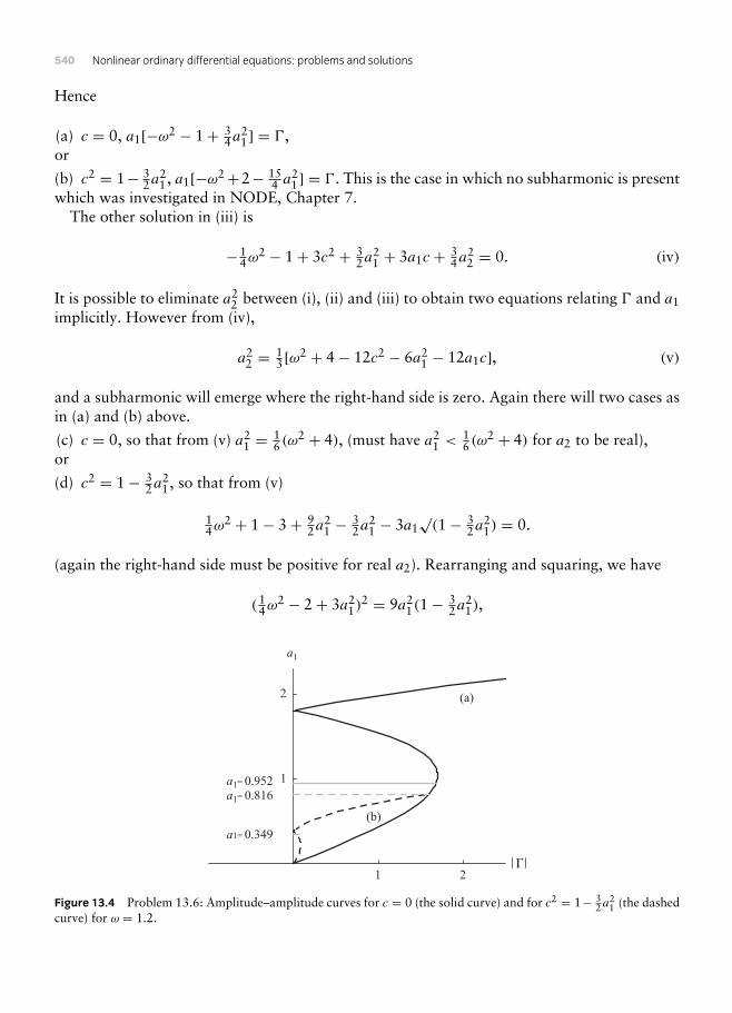
540 Nonlinear ordinary differential equations: problems and solutions
Hence
(a) c = 0, a1[−ω2 − 1+ 34a
21] = ,
or
(b) c2 = 1− 32a
21, a1[−ω2+2− 15
4 a21] = . This is the case in which no subharmonic is present
which was investigated in NODE, Chapter 7.The other solution in (iii) is
−14ω
2 − 1+ 3c2 + 32a
21 + 3a1c + 3
4a22 = 0. (iv)
It is possible to eliminate a22 between (i), (ii) and (iii) to obtain two equations relating and a1
implicitly. However from (iv),
a22 = 1
3 [ω2 + 4− 12c2 − 6a21 − 12a1c], (v)
and a subharmonic will emerge where the right-hand side is zero. Again there will two cases asin (a) and (b) above.
(c) c = 0, so that from (v) a21 = 1
6 (ω2 + 4), (must have a2
1 <16 (ω
2 + 4) for a2 to be real),or
(d) c2 = 1− 32a
21, so that from (v)
14ω
2 + 1− 3+ 92a
21 − 3
2a21 − 3a1
√(1− 3
2a21) = 0.
(again the right-hand side must be positive for real a2). Rearranging and squaring, we have
(14ω
2 − 2+ 3a21)
2 = 9a21(1− 3
2a21),
1 2
1
2
a1
(a)
(b)
a1= 0.952a1= 0.816
a1= 0.349
Figure 13.4 Problem 13.6: Amplitude–amplitude curves for c = 0 (the solid curve) and for c2 = 1− 32a
21 (the dashed
curve) for ω = 1.2.

13 : Poincaré sequences, homoclinic bifurcation, and chaos 541
or
452 a
41 + (3
2ω2 − 27)+ (1
4ω2 − 2)2 = 0, (vi)
from which it is possible to find a1.In our example ω = 1.2. From (c), a2 ≥ 0 where |a1| ≤ 0.9522 on curve (a) in Figure 13.4.
From (d), the solutions of (vi) are |a1| = 0.9911 and |a1| = 0.3488. Real solutions for a2 liebetween these values on curve (b) in Figure 13.4.
• 13.7 Design a computer program to plot 2π/ω first returns for the system x = X(x, y, t),y = Y (x, y, t) where X(x, y, t) and Y (x, y, t) are 2π/ω-periodic functions of t . Apply theprogram to the system
X(x, y, t) = y, Y (x, y, t) = −ky + x − x3 + cosωt ,
for k = 0.3, ω = 1.2 and taking a selection of values between 0 and 0.8. Let the initialsection be t = 0.
13.7. The first returns have been computed using aMathematica program. Consider the Duffingoscillator
x = y, y = −ky + x − x3 + cosωt .
• Parameter values k=0.3, ω=1, =0.2 The first returns starting from x(0)=0.9,y(0)=0.8 are shown in Figure 13.5. The returns approach a fixed point at P whichindicates a stable periodic solution.
• Parameter values k=0.3, ω=1, =0.28. The returns starting from x(0)=0.5, y(0)=0.4but delayed by 15 steps are shown in Figure 13.6. The returns oscillate between two pointsindicating period doubling.
• Parameters k = 0.3, ω = 1, = 0.4. The returns start from x(0) = 0.5, y(0) = 0.4 butare delayed by 10 steps to eliminate transience. The returns are shown in Figure 13.7 andindicate a strange attractor.
0.5 1
0.5
1
x
y0
1
2
3
4
5
P
Figure 13.5 Problem 13.7(i): Poincaré section of period 2π/ω with k = 0.3, ω = 1, = 0.2 and initial valuesx(0) = 0.9, y(0) = 0.8; the successive returns are labelled ‘0’,‘1’,‘2’, . . . and approach the fixed point at P .

542 Nonlinear ordinary differential equations: problems and solutions
0.5 1
0.5
1
x
y
P1
P2
Figure 13.6 Problem 13.7(i): Poincaré section of period 2π/ω with k = 0.3, ω = 1, = 0.28 and initial valuesx(0) = 0.5, y(0) = 0.4; only returns after 15 steps are shown which reveals period doubling between the points P1and P2.
–1 1
–1
1
x
y
Figure 13.7 Problem 13.1(i): Poincaré section of period 2π/ω with k = 0.3, ω = 1, = 0.4 and initial valuesx(0) = 0.5, y(0) = 0.4: the section contains 300 returns indicating a strange attractor.
• 13.8 Find the equations of the stable and unstable manifolds in the (x, y)-plane of
x + x − 2x = 10 cos t , x = yfor Poincaré maps of period 2π and initial time t = 0.
13.8. The general solution of
x + x − 2x = 10 cos t
is
x = Ae−2t + Bet − 3 cos t + sin t .
The fixed point of the system for sections t = 0, period 2π is at (−3, 1) in the (x, y) plane.The stable manifold consists of the set of all points for which B = 0 and t = 2nπ , (n = 0,1, 2, 3, . . . ), that is,
x = Ae−4nπ − 3, y = −2Ae−4nπ + 1.
Elimination of A gives the stable manifold as the line 2x + y + 5 = 0.

13 : Poincaré sequences, homoclinic bifurcation, and chaos 543
The unstable manifold is given by the set of points for which B = 0, that is
x = Be2nπ − 3, y = Be2nπ + 1.
Elimination of B gives the unstable manifold as the line x − y + 4 = 0.
• 13.9 Apply Melnikov’s method to
x + εκx + x3 = εγ (1− x2) cosωωt , κ > 0, ε > 0, γ > 0,
and show that homoclinic bifurcation occurs if, for ω2 2,
|γ | ≥ 2√
2κπω(2− ω2)
cosh(12ωπ).
13.9. The perturbed system is
x + εκx − x + x3 = εγ (1− x2) cosωt .
For ε = 0, the equation x − x + x3 = 0 has the homoclinic solutions x0 = ±√
2 sech t . Weconsider the solution for which x > 0. By NODE, (13.53), the Melnikov function is
M(t0) =∫ ∞
−∞x0(t − t0)[−κx0(t − t0)+ γ 1− x2
0(t − t0)] cosωtdt
= √2γ sinωt0
∫ ∞
−∞sech t tanh t sinωtdt − 2κ
∫ ∞
−∞sech 2
t tanh2tdt
− 2√
2γ sinωt0
∫ ∞
−∞sech 3
t tanh t sinωtdt
= √2γω sinωt0
∫ ∞
−∞sech t cosωtdt − 2κ
∫ ∞
−∞sech 2
t tanh2tdt
− 23
√2γω sinωt0
∫ ∞
−∞sech 3
t cosωtdt .
where we have integrated by parts, and eliminated integrals of odd functions. Now use theknown definite integrals ∫ ∞
−∞sech 2
t tanh2tdt = 2
3 ;
∫ ∞
−∞sech t cosωtdt = πsech (1
2ωπ);
∫ ∞
−∞sech 3
t cosωtdt = 12π(1+ ω2)sech (1
2ωπ).

544 Nonlinear ordinary differential equations: problems and solutions
1 2 3 4
0.5
1k/g
v
Figure 13.8 Problem 13.9: The shaded region indicates possible homoclinic bifurcation.
Finally
M(t0) = 13 [√
2γωπ(2− ω2)sech (12ωπ) sinωt0 − 4κ]. (i)
The Melnikov function for x = −√2sech t is given by (i) with γ replaced by −γ .Homoclinic bifurcation occurs where the Melnikov function vanishes, namely where
√2γωπ(2− ω2)sech (1
2ωπ) sinωt0 = 4κ,
or
sinωt0 = 2√
2κπωγ (2− ω2)
cosh(12ωπ), (ω2 = 2).
It follows that homoclinic bifurcation can only occur if
γ ≥ 2√
2κπω|2− ω2|cosh(1
2ωπ), (ω2 = 2).
The graph of κ/γ against ω is shown in Figure 13.8: the shaded regions indicate possiblehomoclinic bifurcation.
• 13.10 The Duffing oscillator with equation x + εκx − x + x3 = εf (t), is driven by aneven T -periodic function f (t) with mean value zero. Assuming that f (t) can be representedby the Fourier series
∞∑n=1
an cos nωt , ω = 2πT
,
find the Melnikov function for the oscillator.
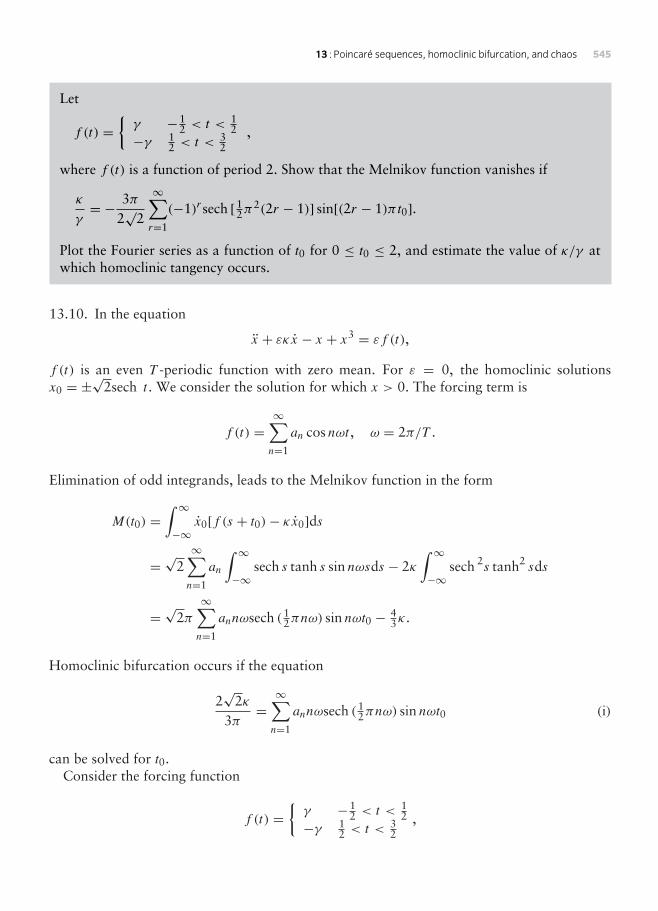
13 : Poincaré sequences, homoclinic bifurcation, and chaos 545
Let
f (t) =γ −1
2 < t <12
−γ 12 < t <
32
,
where f (t) is a function of period 2. Show that the Melnikov function vanishes if
κ
γ= − 3π
2√
2
∞∑r=1
(−1)rsech [12π2(2r − 1)] sin[(2r − 1)πt0].
Plot the Fourier series as a function of t0 for 0 ≤ t0 ≤ 2, and estimate the value of κ/γ atwhich homoclinic tangency occurs.
13.10. In the equation
x + εκx − x + x3 = εf (t),f (t) is an even T -periodic function with zero mean. For ε = 0, the homoclinic solutionsx0 = ±
√2sech t . We consider the solution for which x > 0. The forcing term is
f (t) =∞∑n=1
an cos nωt , ω = 2π/T .
Elimination of odd integrands, leads to the Melnikov function in the form
M(t0) =∫ ∞
−∞x0[f (s + t0)− κx0]ds
= √2∞∑n=1
an
∫ ∞
−∞sech s tanh s sin nωsds − 2κ
∫ ∞
−∞sech 2
s tanh2sds
= √2π∞∑n=1
annωsech (12πnω) sin nωt0 − 4
3κ.
Homoclinic bifurcation occurs if the equation
2√
2κ3π
=∞∑n=1
annωsech (12πnω) sin nωt0 (i)
can be solved for t0.Consider the forcing function
f (t) =γ −1
2 < t <12
−γ 12 < t <
32
,

546 Nonlinear ordinary differential equations: problems and solutions
0.5 1 1.5 2t0
–0.04
–0.02
0.02
0.04
k/g
Figure 13.9 Problem 13.10:
where T = 2 so that ω = π . The Fourier coefficients of f (t) are
a1 = γ
π, a2 = 0, a3 = − γ
3π, a4 = 0, a5 = γ
5π, . . . , (ii)
so that
f (t) = −γπ
∞∑r=1
(−1)r
2r − 1cos(2r − 1)πt .
Substitution of the Fourier coefficients given by (ii) into (i) gives the condition
κ
γ= q(t0) = − 3π
2√
2
∞∑r=1
(−1)rsech [12π2(2r − 1)] sin(2r − 1)πt0 (iii)
for the onset of homoclinic bifurcation. The graph of κ/γ against t0 is shown in Figure 13.9.The first term dominates in the series for q(t0) which accounts for the curve being very close toa sine curve. Hence
κ
γ≈ q(0.5) ≈ 0.048.
• 13.11 Melnikov’s method can be applied also to autonomous systems. The manifoldsbecome the separatrices of a saddle. Let
x + εκx − εx2x + x3 = 0.
Show that the homoclinic path exists to order O(ε2) if κ = 45α. [The following integrals are
required:∫ ∞
−∞sech 4
sds = 43
;∫ ∞
−∞sech 6
sds = 1615
].
13.11. Consider the autonomous equation
x + εκx − εαx2x − x + x3 = 0.

13 : Poincaré sequences, homoclinic bifurcation, and chaos 547
The Melnikov function is given by
M(t0) =∫ ∞
−∞x0(t)(αx
20 x0 − κx0)dt ,
where, for ε = 0, x0 =√
2 sech t . Therefore
M(t0) = 2∫ ∞
−∞sech 2
t tanh2t(2αsech 2
t − κ)dt
= 4α∫ ∞
−∞sech 4
t tanh2tdt − 2κ
∫ ∞
−∞sech 2
t tanh2tdt
= 4α∫ ∞
−∞sech 4
tdt − 4α∫ ∞
∞sech 6
tdt − 43κ
= 16α3− 64α
15− 4κ
3= 16α
15− 4κ
3
Hence M(t0) = 0 where κ = 4α/5.
• 13.12 Show that x = 31/4√(sech 2t) is a homoclinic solution of x+ε(κ−αx2)x−x+x5 = 0when ε = 0. Use Melnikov’s method to show that homoclinic bifurcation occurs whenκ = 4
√3α/(3π).
13.12. The given equation is
x + ε(κ − αx2)x − x + x5 = 0.
Let x0 = 31/4√(sech 2t). Then
x0 − x0 + x50 = 31/4[−2
√(sech 2t)+ 3sech 5/22t sinh2 2t] − 31/4√(sech 2t)+ 35/4(sech 2t)5/2
= 0,
which confirms that x0(t) is a homoclinic solution of the unperturbed system. The Melnikovfunction is given by
M(t0) =∫ ∞
−∞x0(αx
20 x0 − κx0)dt .

548 Nonlinear ordinary differential equations: problems and solutions
Hence
M(t0) =√
3∫ ∞
−∞sech 32t sinh2 2t[α√3sech 2t − κ]dt
= 3α∫ ∞
−∞sech 42t sinh2 2tdt − κ√3
∫ ∞
−∞sech 32t sinh2 2tdt
= 3α∫ ∞
−∞[sech 22t − sech 42t]dt − κ√3
∫ ∞
−∞[sech 2t − sech 32t]dt
= 3α(1− 23 )− κ
√3(1
2π − 14π)
= α − 14κπ
√3.
Therefore a homoclinic bifurcation first occurs where κ ≈ 4√
3α/(3π).
• 13.13 Apply Melnikov’s method to the perturbed system x + εκx − x + x3 = εγ x cosωt ,which has an equilibrium point at x = 0 for all t . Show that the manifolds of the originintersect if
γ ≥ 4κ3ω2π
sinh(12ωπ).[
Hint :∫ ∞
−∞sech 2
u cosωudu = πω
sinh(12ωπ)
.
]
13.13. In the Duffing type oscillator
x + εκx − x + x3 = εγ x cosωt , x = y
the forcing term depends also on x. In the solution of the problem it is assumed that ε > 0,κ > 0 and γ > 0. The unperturbed solution is the familiar x0 =
√2sech t . The Melnikov
function is given by
M(t0) =∫ ∞
−∞y0(t − t0)h(x0(t − t0), y0(t − t0), t)dt
=∫ ∞
−∞y0(s)h(x0(s), y0(s), s + t0)ds,
after a change of variable, where h(x, y, t) = −κy + γ x cosωt . Therefore
M(t0) = −κ∫ ∞
−∞y2
0(s)ds + γ∫ ∞
−∞y0(s)x0(s) cos(ωs + t0)ds
= −κ∫ ∞
−∞y2
0(s)ds − γ∫ ∞
−∞y0(s)x0(s) sinωs sinωt0ds,

13 : Poincaré sequences, homoclinic bifurcation, and chaos 549
since x0 is an even function. Substitution for x0 gives
M(t0) = −2κ∫ ∞
−∞sech 2
s tanh2sds + 2γ sinωt0
∫ ∞
−∞sech 2
s tanh s sinωsds
= −2κ∫ ∞
−∞[sech 2
s − sech 4s]ds − γ sinωt0
∫ ∞
∞dds(sech 2
s) sinωsds
= −2κ(2− 43 )+ γω sinωt0
∫ ∞
−∞sech 2
s cosωsds
= −43κ + γω2π
sinh(12ωπ)
.
The stable and unstable manifolds of the origin intersect if M(t0) ≥ 0, that is, if
γ ≥ 4κ3ω2π
sinh(12ωπ).
• 13.14 Show that the logistic difference equation un+1 = λun(1 − un) has the generalsolution un = sin2(2nCπ) if λ = 4, where C is an arbitrary constant (without loss C canbe restricted to 0 ≤ C ≤ 1). Show that the solution is 2q -periodic (q any positive integer) ifC = 1/(2q − 1). The presence of all these periodic doubling solutions indicates chaos. (Seethe article by Brown and Chua (1996) for further exact solutions of nonlinear differenceequations relevant to this and succeeding problems.)
13.14. In the difference equation
un+1 = λun(1− un),
let un = sin2(2nCπ). Then
λun(1− un) = λ sin2(2nCπ)(1− sin2(2nCπ)) = λ sin2(2nCπ) cos2(2nCπ)
= 14λ sin2(2n+1Cπ) = un+1
if λ = 4. Hence un = sin2(2nCπ) is an exact solution. It is sufficient that 0 ≤ C ≤ 1.A period q solution exists if C satisfies
un = un+q , or sin2(2nCπ) = sin2(2n+qCπ).
where q is a positive integer. Therefore C must satisfy
cos(2n+1Cπ)− cos(2n+1+qCπ) = 0,

550 Nonlinear ordinary differential equations: problems and solutions
or
sin[2nCπ(2q + 1)] sin[2nCπ(2q − 1)] = 0.
Hence a period q solution exists if C = 1/(2q − 1). Hence these solutions exist for all q whichimplies that the solution is chaotic.
• 13.15 Show that the difference equation un+1 = 2u2n − 1 has the exact solution un =
cos(2nCπ)whereC is any constant satisfying 0 ≤ C ≤ 1. For what values ofC do q-periodicsolutions exist?
13.15. In the difference equationun+1 = 2u2
n − 1,
let un = cos(2nCπ). Then
2u2n − 1 = 2 cos2(2nCπ)− 1 = cos(2n+1cπ) = un+1.
Hence un = cos(2nCπ) is an exact solution.A period q solution exists if C satisfies
un = un−q , or cos(2nCπ) = cos(2n+qCπ),
or
sin[Cπ(2n−1+q + 2n−1)] sin[Cπ(2n−1+q − 2n−1)] = 0.
Since C is independent of n, period q solutions exist if
C = 12q + 1
, or C = 12q − 1
, (q ≥ 1).
• 13.16 Using a trigonometric identity for cos 3t , find a first-order difference equationsatisfied by un = cos(3nCπ).
13.16. Problems 13.14, 13.15 and this problem follow from trigonometric identities for multi-ple angles. In this case we require a difference equation which has the solution un = cos(3nCπ).Consider the identity
cos 3u = 4 cos3 u− 3 cos u.
If we put u = 3nCπ , it follows that
un+1 = 4u3n − 3un.

13 : Poincaré sequences, homoclinic bifurcation, and chaos 551
• 13.17 A large number of phase diagrams have been computed and analysed for the two-parameter Duffing equation
x + kx + x3 = cos t , x = yrevealing a complex pattern of periodic, subharmonic and chaotic oscillations (see Ueda(1980) for an extensive catalogue of outputs, and also Problem 7.32). Using a suitablecomputer package plot phase diagram and time solutions in each of the following cases forthe initial data given, and discuss the type of solutions in each generated:
(a) k = 0.08, = 0.2; x(0) = −0.205, y(0) = 0.0171; x(0) = 1.050, y(0) = 0.780.
(b) k = 0.2, = 5.5; x(0) = 2.958, y(0) = 2.958; x(0) = 2.029, y(0) = −0.632.
(c) k = 0.2, = 10; x(0) = 3.064, y(0) = 4.936.
(d) k = 0.1, = 12; x(0) = 0.892, y(0) = −1.292.
(e) k = 0.1, = 12; x(0) = 3, y(0) = −1.2.
13.17. The equationx + kx + x3 = cos t
has been analysed numerically in some detail by Ueda (1980). Here we display cases (a), (d)and (e) for various initial values.
• (a) k=0.08, =0.2, with two sets of initial values x0 = −0.205, y0=0.0171 andx0=1.050, y0=0.780. These initial values generate approximately two co-existing stable2π -periodic solutions which are shown in Figure 13.10. The time solutions of the twoperiods are shown in Figure 13.11.
• (d) k=0.1, =12, with initial values x0=0.892, y0 = −1.292. These initial valuesgenerate a 2π periodic solution shown in Figure 13.12. The time solution is shown inFigure 13.13.
• (e) k=0.1, =12, with initial values x0=3, y0=1.2. These initial values generate achaotic response shown in Figure 13.14. The parameter values are the same as those incase (d) so that this chaotic solution co-exists with the periodic solution shown in (d). Thetime solution is shown in Figure 13.15.
–1 1x
–1
1
y
Figure 13.10 Problem 13.17(a): Ueda’s equation with k = 0.08, = 0.2, and the two sets of initial values x0 =−0.205, y0 = 0.0171 and x0 = 1.050, y0 = 0.780.

552 Nonlinear ordinary differential equations: problems and solutions
2 4t
–1
1
x
Figure 13.11 Problem 13.17: Periodic time solutions with k = 0.08, = 0.2.
–4 –2 2 4x
–4
–2
2
4
y
Figure 13.12 Problem 13.17: Ueda’s equation with k = 0.1, = 12, and the initial values x0 = 0.892, y0 = −1.292.
2 4t
–1
1
x
Figure 13.13 Problem 13.17: Periodic time solution with k = 0.1, = 12.
–4 4x
–10
10y
Figure 13.14 Problem 13.17: Ueda’s equation with k = 0.1, = 12, and the initial values x0 = 3, y0 = 1.2.

13 : Poincaré sequences, homoclinic bifurcation, and chaos 553
36t
–4
4
x
Figure 13.15 Problem 13.17: Periodic time solutions with k = 0.1, = 12.
• 13.18 Consider the Hamiltonian system
pi = −∂H∂qi
, qi = ∂H
∂pi, (i = 1, 2)
where H = 12ω1(p
21 + q2
1 )+ 12ω2(p
22 + q2
2 ). Show that q1, q2 satisfy the uncoupled system
qi + ω2i qi = 0, (i = 1, 2).
Explain why the ellipsoids12ω1(p
21 + q2
1 )+ 12ω2(p
22 + q2
2 ) = constant
are invariant manifolds in the four-dimensional space (p1,p2, q1, q2). What condition onω1/ω2 guarantees that all solutions are periodic? Consider the phase path which satisfiesp1 = 0, q1 = 0, p2 = 1, q2 = 0. Describe the Poincaré section p1 = 0 of the phase pathprojected on to the (q1,p2, q2) subspace.
13.18. Consider the mechanical system
pi = −∂H∂qi
, qi = ∂H
∂pi, (i = 1, 2),
where H = 12ω1(p
21 + q2
1 )+ 12ω2(p
22 + q2
2 ). The equations of motion are
p1 = −ω1q1, q1 = ω1p1, p2 = −ω2q2, q2 = ω2p2,
or, equivalently,q1 + ω2
1q1 = 0, q2 + ω22q2 = 0.
The solutions are
q1 = A1 cosω1t + B1 sinω1t , q2 = A2 cosω2t + B2 sinω2t .
These solutions are periodic if ω1/ω2 is a rational number. If this ratio is not rational then q1and q2 are uncoupled with periods 2π/ω1 and 2π/ω2.

554 Nonlinear ordinary differential equations: problems and solutions
Phase paths in p1, q1, p2, q2 space are given by
dp1
dq1= − q1
p1⇒ p2
1 + q21 = C1, (i)
dp2
dq2= − q2
p2⇒ p2
2 + q22 = C2. (ii)
Also
H = 12ω1(p
21 + q2
1 )+ 12ω2(p
22 + q2
2 ) = constant.
Therefore any path which starts on this surface will stay on it, which means that the ellipsoidsH = constant are invariant manifolds.
Consider the path for which the initial conditions p1 = 0, q1 = 0, p2 = 1, q2 = 0. In (i) and(ii) C1 = 0 and C2 = 1. Therefore the projection of the manifold on to the (q1,p2, q2) subspaceare the straight lines p2 = q2 = 0, p2 = ±1.
• 13.19 Consider the system
x = −ryz, y = rxz, z = −z+ cos t − sin t ,
where r = √(x2 + y2). Show that, projected on to the (x, y) plane, the phase paths havethe same phase diagram as a plane centre. Show also that the general solution is given by
x = x0 cosω(t)− y0 sinω(t), y = y0 cosω(t)+ x0 sinω(t), z = z0e−t + sin t .
where ω(t) = r0[1 − cos t + z0(1 − e−t )], and x0 = x(0), y0 = y(0) z0 = z(0), andr0 = √(x2
0 + y20). Confirm that, as t →∞, all solutions become periodic.
13.19. Consider the forced system
x = −ryz, y = rxz, z = −z+ cost − sin t , r = √(x2 + y2).
From the first two equations,
dydx= −x
y⇒ x2 + y2 = c2,
say (assume c ≥ 0). Hence, projected on to the x, y plane, the phase paths are the same as thoseof simple harmonic motion.
Integration of the equation for z leads to the solution
z = z0e−t + sin t ,
where z(0) = z0. Hencex = −c(z0e−t + sin t)
√(c2 − x2).

13 : Poincaré sequences, homoclinic bifurcation, and chaos 555
This separable equation has the general solution
x = c sin(z0ce−t + c cos t + B).
Alsoy = c cos(z0ce−t + c cos t + B).
From the initial conditions
x0 = r0 sin(z0r0 + r0 + B), y0 = r0 cos(z0r0 + r0 + B).
Thereforex = x0 cosω(t)− y0 sinω(t), y = y0 cosω(t)+ x0 sinω(t),
whereω(t) = r0[1− cos t + z0(1− e−t )].
As t →∞,
z→ sin t , x → c sin(c cos t + B), y → c cos(c cos t + B),
which are all periodic with period 2π in t .
• 13.20 A common characteristic feature of chaotic oscillators is sensitive dependence oninitial conditions, in which bounded solutions which start very close together utimatelydiverge. Such solutions locally diverge exponentially. Investigate time-solutions of Duffing’sequation
x + kx − x + x3 = cosωt
for k = 0.3, = 0.5, ω = 1.2, which is in the chaotic parameter region (see Figure 13.15in NODE), for the initial values (a) x(0) = 0.9, y(0) = 0.42; (b) y(0) = 0.42 but with avery small increase in x(0) to say 0.90000001. Divergence between the solutions occurs atabout 40 cycles. (Care must be exercised in computing solutions in chaotic domains wheresensitive dependence on initial values and computation errors can be comparable in effect.)
13.20. Consider the Duffing equation
x + kx − x + x3 = cosωt ,
subject to slightly differing initial conditions. Figure 13.16 shows the numerical solution ofthe equation with the parameters k=0.3, =0.5 and ω=1.2 for the initial conditions (a)x(0)=0.90, y(0)=0.42, denoted by x1; (b) x(0)=0.90000001, y(0)=0.42, denoted by x2.The difference between the numerical solutions is shown in the third graph. After about 28cycles the solutions start to diverge.

556 Nonlinear ordinary differential equations: problems and solutions
100 t
–1
1
x1 – x2
100 t
–1
1
x2
100 t
–1
1
x1
Figure 13.16 Problem 13.20:
• 13.21 The Lorenz equations are given by (see Problem 8.26 and Section 13.2 in NODE)
x = a(y − x), y = bx − y − xz, z = xy − cz,Compute solutions of these equations in (x, y, z) phase space. Chaotic solutions appearnear parameter values a = 10, b = 27, c = 2.65: a possible initial state is x(0) = −11.720,y(0) = −17.249, z(0) = 22.870.
13.21. The Lorenz equations are given by
x = a(y − x), y = bx − y − xz, z = xy − cz.
For the parameters a = 10, b = 27, c = 2.65, a single phase path is shown in Figure 13.17.Over long runs the solution continues to display chaotic behaviour.
x
y
z
Figure 13.17 Problem 13.21: A single phase path for Lorenz equation x = a(y − x), y = bx − y − xz, z = xy − czwith a = 10, b = 27, c = 2.65.

13 : Poincaré sequences, homoclinic bifurcation, and chaos 557
• 13.22 Show that the system x = −y+ sin t , y = −x+2x3+ cos t , ( > 0), has a limitcycle x = 0, y = sin t . Find also the time-solutions for x and y of the paths which arehomoclinic to this limit cycle. Sketch the phase paths of the limit cycle and the homoclinicpaths for = 1.
13.22. In the system
x = −y + sin t , y = −x + 2x3 + cos t ,
it can be seen that x = 0, y = sin t is a solution. This is obviously a periodic solution of thesystem.
Let y = sin t + z. Thenx = z, z = x − 2x3.
Hence, eliminating z,x = x − 2x3.
We can verify that this equation has the solution x = sech t , which has the required propertythat x → 0 as t →±∞. Therefore
y = sin t − z = sin t − x = sin t + sech 2t sinh t .
The homoclinic path is
x = sech t , y = sin t + sech 2t sinh t .
Similarly there is a complementary path
x = −sech t , y = sin t − sech 2t sinh t .
The homoclinic path in the half-plane x ≥ 0 is shown in Figure 13.18. The periodic solutionlies on the y axis between y = and y = −. The homoclinic path for this forced system startson the periodic solution and ends there.
0.5 1x
–1
1
y
Figure 13.18 Problem 13.22: Homoclinic path x = sech t , y = sin t + sech 2t sinh t with = 1.

558 Nonlinear ordinary differential equations: problems and solutions
–2 –1 1 2x
–1
1
y(a)
P–2 –1 1 2
x
–1
1
y(b)
P1
P2
Figure 13.19 Problem 13.23: (a) Fixed point of x = cos t , for t0 = 0 and period T = 2π ; (b) period doubling forx = 3 cos 1
2 t with t0 = 12π and period T = 2π .
• 13.23 For each of the following functions and solutions plot the Poincaré sequence in thex, y = x plane, starting with the given initial time t0 and given period T .
(a) x = 2 cos t ; t0 = 0, T = 2π .
(b) x = 3 cos t ; t0 = 12π , T = 2π .
(c) x = sin t + sinπt ; t0 = 12π , T = 2π .
(d) The periodic solution of x − (x2 + x2)x + x = cos t , where t0 = 0, T = 2π .
13.23. (a) For x = 2 cos t , y = x = −2 sin t . Therefore if t0 = 0, then
x(2nπ) = 2 cos 2nπ = 2, y(2nπ) = −2 sin 2nπ = 0.
In this section the function has a fixed point at (2, 0) shown as P in Figure 13.19(a).(b) For x = 3 cos 1
2 t , y = x = −32 sin 1
2 t . If t0 = 12π and T = 2π , then
x(2n+ 12π) = 3 cos[(n+ 1
4 )π ] =
3/√
2 n even−3/
√2 n odd
,
y(2n+ 12π) = −3
2 sin[(n+ 14 )π ] =
−3/(2√
2) n even3/(2
√2) even
In this section the solution oscillates between the two fixed points at [3/√2,−3/(2√
2)] and[−3/
√2, 3/(2
√2)] shown as P1 and P2 in Figure 13.19(b). In this section the function exhibits
period doubling.(c) For x = sin t + sinπt , y = cos t + π cos t . The function sin t + sinπt is not periodic. Witht0 = 1
2π and T = 2π ,
x0 = x(12π) = 1+ sin 1
2π2, y0 = y(1
2π) = π cos 12π
2,
xn = x[(2n+ 12 )π ] = 1+ sin[(2n+ 1
2 )π2],
yn = y[(2n+ 12 )π ] = π cos[(2n+ 1
2 )π2].

13 : Poincaré sequences, homoclinic bifurcation, and chaos 559
All these points lie on the ellipse
(x − 1)2 + y2
π2 = 1,
but there are no repetitions of points.(d) In the equation
x − (x2 + x2)x + x = cos t ,
Let x = A cos t . Then
x − (x2 + x2)x + x − cos t = −A cos t − A2(−A cos t)+ A cos t − cos t
= (A3 − 1) cos t = 0,
if A = 1. With t0 = 0 and T = 2π , the periodic solution has a fixed point at (1, 0).
• 13.24 Show that x + k(1− x2 − x2)2x − x = −2 cos t has a limit cycle whose solution isx0 = cos t . By looking at perturbations x = x0 + x′ where |x′| is small show that the limitcycle has Poincaré fixed points which are saddles.
13.24. In the forced equation
x + k(1− x2 − x2)2x − x = −2 cos t ,
let x = A cos t . Then
x + k(1− x2 − x2)2x − x + 2 cos t = −A cos t − k(1− A2)2A sin t − A cos t + 2 sin t
= 2(1− A) cos t − k(1− A2)A sin t = 0
if A = 1. Therefore x = x1 = cos t is a limit cycle. For any t0 and period 2π , the limit cycle hasthe fixed point (cos t0,− sin t0).
Let x = x1 + x′. The linearized equation for x′ is
x′ − x′ = 0,
which has the general solution
x′ = Bet + Ce−t .
Since this solution has stable and unstable manifolds the fixed points are saddles.

560 Nonlinear ordinary differential equations: problems and solutions
• 13.25 Consider the system x = y, y = (e−2x − e−x) + ε cos t . For ε = 0, show thatthe equations of its phase paths is given by y2 = 2e−x − e−2x + C. Show that the systemhas closed paths about the origin if −1 < C < 0 with a bounding separatrix given byy2 = 2e−x − e−2x . What happens to paths for C > 0? Sketch the phase diagram.Suppose that the system is moving along the separatrix path, and at some instant the forcingis introduced. Describe what you expect the behaviour of the system to be after the intro-duction of the forcing. Compute a Poincaré sequence and a time-solution for ε = 0.5 andfor the initial conditions, x(0) = − ln 2, y(0) = 0.
13.25. The differential equation for the phase paths of
x = y, y = (e−2x − e−x)
isdydx= e−2x − e−x
y,
which has the general solution
y2 = −(e−2x − 2e−x)+ C.
This autonomous system has one equilibrium point at (0, 0).We can determine where paths cut the x axis by putting y = 0, in which case
e−2x − 2e−x − C = 0, or e−x = 1±√(1+ C). (i)
Two real solutions for x occur if −1 < C < 0. Since the paths are reflected in the x axis, thisimplies that closed paths enclose the origin which is a centre. If C = 0, then x = − ln 2 is onesolution but for the other x →∞ as C → 0−. The bounding path of the centre is
y2 = −e−2x + e−x .
which is the dashed path in the phase diagram shown in Figure 13.20. If C >0, then pathsapproach y=√(2C) as x→∞, and approach y = −√(2C) as x→ −∞.
If forcing is introduced at the point (− ln 2, 0) (on the separatrix), we might expect thesolution to oscillate between the stable centre and the unbounded paths but with x progressivelyincreasing. Since the width of the centre decreases with x we might also expect the solution tobecome unbounded in x. The particular path which starts at (− ln 2, 0) is shown in Figure 13.21,and confirms the prediction.

13 : Poincaré sequences, homoclinic bifurcation, and chaos 561
–1 1x
–1
1
y
Figure 13.20 Problem 13.25: Phase diagram for x = y, y = e−2x − e−x : the dashed path separates the centre fromunbounded paths.
–1 10x
–2
–1
1
2
y
5
Figure 13.21 Problem 13.25:
• 13.26 Apply the change of variable z = u+ a + b to the Lorenz system
x = a(y − x), y = bx − y − xz, z = xy − cz,where a, b, c > 0. If s = √(x2 + y2 + z2), show that
12s
dsdt= −ax2 − y2 − c[u+ 1
2 (a + b)]2 + 14c(a + b)2.
What is the sign of ds/dt on the ellipsoid ax2 + y2 + c[u + 12 (a + b)]2 = ρ (*), where
ρ > 14c(a + b)2?
Show that all equilibrium points are unstable in the case a = 4, b = 34, c = 12 . If this
condition is satisfied, what can you say about the attracting set inside the ellipsoid (*) if ρis sufficiently large?
13.26. Apply the change of variable z = u+ a + b to the Lorenz system
x = a(y − x), y = bx − y − xz, z = xy − cz, (a, b, c > 0). (i)
Thenx = a(y − x), y = −y − x(u+ a), u = xy − c(u+ a + b).

562 Nonlinear ordinary differential equations: problems and solutions
Let s = √(x2 + y2 + z2). Then
sdsdt= xx + yy + zz= xa(y − x)− y2 − xy(u+ a)+ uxy − u(u+ a + b)c= −ax2 − y2 − c[u+ 1
2 (a + b)]2 + 14c(a + b)2
On the ellipsoidax2 + y2 + c[u+ 1
2 (a + b)]2 = ρ, (ii)
sdsdt= −ρ + 1
4c(a + b)2 < 0
if ρ > 14c(a + b)2 = ρ1, say.
From (i), the Lorenz equations have equilibrium points in the (x, y, u) space given by
x = y, bx − y − xz = 0, xy − cz = 0.
• b ≤ 1. The system has one equilibrium point at (0, 0,−a − b).• b > 1. Equilibrium occurs at the points
(0, 0,−a − b), (√c√(b − 1),
√c√(b − 1),−a − 1),
(−√c√(b − 1),−√c√(b − 1),−a − 1).
The equilibrium point (0, 0,−a − b) lies on the ellipsoid
ax2 + y2 + c[u+ 12 (a + b)]2 = 1
4c(a + b)2 = ρ1,
that is, this equilibrium point lie on the critical ellipsoid. Hence this point always lies withinthe ellipsoid defined by (ii) with ρ > ρ1.
The point (√c√(b − 1),
√c√(b − 1),−a − 1) lies on the ellipsoid
ax2 + y2 + c[u+ 12 (a + b)]2 = 1
4c(a2 + 2b2 + 2ab).
Since 14c(a
2+2b2+2ab)> 14c(a+ b)2= ρ1, this equilibrium point lies outside the ellipsoid with
ρ= ρ1. The point (−√c√(b − 1),−√c√(b − 1),−a − 1) lies on the same ellipsoid.The linearized equations associated with the equilibrium points are as follows.
• (0, 0,−a − b). If u = −a − b + u′, the linearized equations are
x = −ax + ay, y = (a + 2b)x − y, u′ = −cu.

13 : Poincaré sequences, homoclinic bifurcation, and chaos 563
The eigenvalues are given by
∣∣∣∣∣∣−a − λ a 0a + 2b −1− λ 0
0 0 −c − λ
∣∣∣∣∣∣ = −(λ− c)[λ2 + (a + 1)λ− a2 − 2ab] = 0.
Since one solution for λ is positive this equilibrium point is unstable for all b > 0.• (√c√(b − 1),
√c√(b − 1),−a−1), (b > 1). Let x = √c√(b − 1)+x′, y=√c√(b − 1)+y′
and u= − a − 1+ u′. The linearized equations are
x′ = −ax′ + ay′, y′ = (b + 1)x′ − y′ − √c√(b − 1)u′, .
u′ = √c√(b − 1)x′ + √c√(b − 1)y′ − cu′.
The eigenvalues are given by
∣∣∣∣∣∣−a − λ a 0b + 1 −1− λ −√c√(b − 1)√c√(b − 1)
√c√(b − 1) −c − λ
∣∣∣∣∣∣ = 0,
or
λ3 + (a + c + 1)λ2 + c(a + b)λ+ 2ac(b − 1) = 0.
If a = 4, b = 34, c = 12 , then λ satisfies
2λ3 + 11λ2 + 38λ+ 264 = (λ+ 6)(2λ2 − λ+ 44) = 0.
This equation has the solution λ= − 6, and two complex solutions which have positivereal part. Therefore this equilibrium point is unstable.
• (−√c√(b − 1),−√c√(b − 1),−a − 1), (b > 1). It can be shown that this equilibriumpoint has the same eigenvalues as the previous case.
For the given values of a, b and c there are three equilibrium points all of which are unstable.Also there is an ellipsoid (ii) which encloses these equilibrium points, and such that allphase paths pass from the outside to the inside to the outside. Hence subsequently any pathwhich crosses the ellipsoid either approaches a limit cycle or wanders indefinitely inside theellipsoid.

564 Nonlinear ordinary differential equations: problems and solutions
• 13.27 A plane autonomous system is governed by the equation x = X(x, y), y = Y (x, y).Consider a set of solutions x(t , x0, y0), y(t , x0, y0) which start at time t = t0 at (x0, y0),where (x0, y0) is any point in a region D(t0) bounded by a smooth simple closed curve C.At time t , D(t0) becomes D(t). The area of D(t) is
A(t) =∫ ∫
D(t)dxdy =
∫ ∫D(t0)
dx0dy0
when expressed in terms of the original region. In this integral, the Jacobian J (t) =det((t)), where
(t) =
∂x
∂x0
∂x
∂y0∂y
∂y0
∂y
∂y0
.
Show that (t) satisfies the linear equation (t) = B(t)(t), (note that (t) is a fundamentalmatrix of this equation) where
B(t) =∂X
∂x
∂X
∂y∂Y
∂x
∂Y
∂y
.
Using Theorem 9.4 (on a property of the Wronskian), show that
J (t) = J (t0) exp[∫ t
t0
(∂X
∂x+ ∂Y
∂y
)ds
].
If the system is Hamiltonian deduce that J (t) = J (t0). What can you say about the areaof D(t)? (A(t) is an example of an integral invariant and the result is known as Liouville’stheorem.)For an autonomous system in n variables x = X(x), what would you expect thecorresponding condition for a volume-preserving phase diagram to be?
13.27. The plane autonomous system is x = X(x, y), y = Y (x, y). Consider the set of solutionsx(t , x0, y0), y(t , x0, y0) which start at time t = t0 at (x0, y0), where (x0, y0) is any point ina region D(t0) bounded by a smooth simple C. At time t , D(t0) becomes D(t) as shown inFigure 13.22. Let A(t) be the area of D(t) so that
A(t) =∫ ∫
D(t)dxdy.
The region D(t) is obtained from D(t0) by the change of variable x = x(t , x0, y0), y =y(t , x0, y0). In terms of the original region
A(t) =∫ ∫
D(t)dxdy =
∫ ∫D(t0)
J (t)dxdy,

13 : Poincaré sequences, homoclinic bifurcation, and chaos 565
x
y
D(t0)
D (t)
Figure 13.22 Problem 13.27:
where J (t) is the JacobianJ (t) = det((t)),
where
(t) =
∂x
∂x0
∂x
∂y0∂y
∂x0
∂y
∂y0
.
The derivative
(t) =
∂x
∂x0
∂x
∂y0∂y
∂x0
∂y
∂y0
=
∂X
∂x0
∂X
∂y0∂Y
∂x0
∂Y
∂y0
=∂X
∂x
∂x
∂x0+ ∂X
∂y
∂y
∂x0
∂X
∂x
∂x
∂y0+ ∂X
∂y
∂y
∂y0∂Y
∂x
∂x
∂x0+ ∂Y
∂y
∂y
∂x0
∂Y
∂x
∂x
∂y0+ ∂Y
∂y
∂y
∂y0
=∂X
∂x
∂X
∂y∂Y
∂x
∂Y
∂y
∂x
∂x0
∂y
∂x0∂y
∂x0
∂y
∂y0
= B(t)(t)
where
B(t) =∂X
∂x
∂X
∂y∂Y
∂x
∂Y
∂y
.
By NODE, Theorem 9.4,
(t) = (t0) exp[∫ t
t0
tr[B(s)]ds]= (t0) exp
[∫ t
t0
∂X
∂x+ ∂Y
∂y
ds
].

566 Nonlinear ordinary differential equations: problems and solutions
Finally
J (t) = det[(t)] = det[(t0)] exp[∫ t
t0
∂X
∂x+ ∂Y
∂y
ds
]
= J (t0) exp[∫ t
t0
∂X
∂x+ ∂Y
∂y
ds
]. (i)
If the system is Hamiltonian, then
∂X
∂x+ ∂Y
∂y= 0,
so that (i) becomes J (t) = J (t0) = 1. Therefore A(t) = A(t0), which means that area ispreserved for all t .
An n dimensional autonomous system is volume-preserving if tr(B) = 0.
• 13.28 For the more general version of Liouville’s theorem (see Problem 13.27) appliedto the case n = 3 with x = X(x, y, z), y = Y (x, y, z), z = Z(x, y, z), the volume of a regionD(t) which follows the phase paths is given by
W(t) =∫ ∫ ∫
D(t)dxdydz =
∫ ∫ ∫D(t0)
J (t)dx0dy0dz0,
where the Jacobian J (t) = det[(t)]. As in the previous problem
J (t) = J (t0) exp[∫ t
t0
(∂X
∂x+ ∂Y
∂y+ ∂Z
∂z
)ds
].
Show that dJ (t)/dt → 0 as t →∞ for the Lorenz system
x = a(y − x), y = bx − y − xz, z = xy − cz,where a, b, c > 0. What can be said about the volume of any region following phase pathsof the Lorenz attractor as time progresses?
13.28. For the system x = X(x, y, z), y = Y (x, y, z), z = Z(x, y, z), the volume of a region D(t)which follows the phase paths is given by
W(t) =∫ ∫ ∫
D(t)dxdydz =
∫ ∫ ∫D(t0)
J (t)dx0dy0dz0,

13 : Poincaré sequences, homoclinic bifurcation, and chaos 567
where
J (t) = det[(t)], (t) =
∂x
∂x0
∂x
∂y0
∂x
∂z0∂y
∂x0
∂y
∂y0
∂y
∂z0∂z
∂x0
∂z
∂y0
∂z
∂z0
.
It can be shown using a method which parallels that given in the previous problem that
J (t) = J (t0) exp[∫ t
t0
(∂X
∂x+ ∂Y
∂y+ ∂Z
∂z
)ds
].
A system will be volume-preserving if
∂X
∂x+ ∂Y
∂y+ ∂Z
∂z= 0.
For the Lorenz system
x = a(y − x), y = bx − y − xz, z = xy − cz,
∂X
∂x+ ∂Y
∂y+ ∂Z
∂z= ∂[a(y − x)]
∂x+ ∂[bx − y − xz]
∂y+ ∂[xy − cz]
∂z
= −a − 1− c < 0.
Therefore
J (t) = J (t0) exp[∫ t
t0
(∂X
∂x+ ∂Y
∂y+ ∂Z
∂z
)ds
]= J (t0)e−(a+c+1)t → 0
as t →∞.
• 13.29 Show that x(1 + x) − xx − x = −2γ (x + 1) cos t , (γ > 0) has the exact solutionx = Aet + Be−t + γ cos t . What can you say about the stability of the limit cycle? Find thePoincaré sequences of the stable and unstable manifolds associated with t = 0 and period2π . Write down their equations and sketch the limit cycle, its fixed Poincaré point and thestable and unstable manifolds.
13.29. Let x = Aet + Be−t + γ cos t . Then
x(1+ x)− xx − x + 2γ (x + 1) cos t = (1+ x)(x − x + 2γ cos t) = 0.
Therefore x = Aet + Be−t + γ cos t is an exact solution. The limit cycle is unstable.
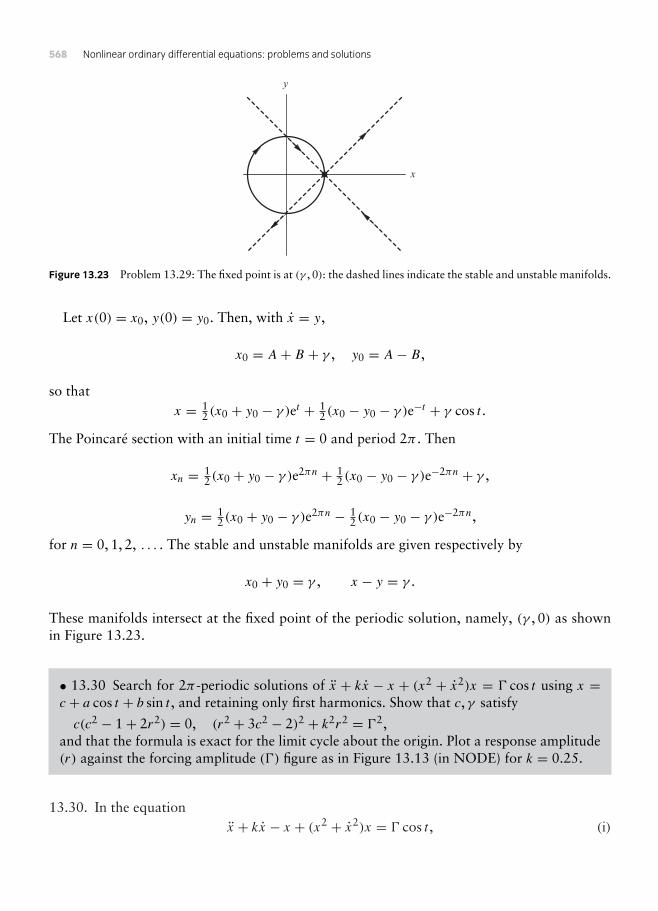
568 Nonlinear ordinary differential equations: problems and solutions
x
y
Figure 13.23 Problem 13.29: The fixed point is at (γ , 0): the dashed lines indicate the stable and unstable manifolds.
Let x(0) = x0, y(0) = y0. Then, with x = y,
x0 = A+ B + γ , y0 = A− B,
so thatx = 1
2 (x0 + y0 − γ )et + 12 (x0 − y0 − γ )e−t + γ cos t .
The Poincaré section with an initial time t = 0 and period 2π . Then
xn = 12 (x0 + y0 − γ )e2πn + 1
2 (x0 − y0 − γ )e−2πn + γ ,
yn = 12 (x0 + y0 − γ )e2πn − 1
2 (x0 − y0 − γ )e−2πn,
for n = 0, 1, 2, . . . . The stable and unstable manifolds are given respectively by
x0 + y0 = γ , x − y = γ .
These manifolds intersect at the fixed point of the periodic solution, namely, (γ , 0) as shownin Figure 13.23.
• 13.30 Search for 2π -periodic solutions of x + kx − x + (x2 + x2)x = cos t using x =c + a cos t + b sin t , and retaining only first harmonics. Show that c, γ satisfy
c(c2 − 1+ 2r2) = 0, (r2 + 3c2 − 2)2 + k2r2 = 2,and that the formula is exact for the limit cycle about the origin. Plot a response amplitude(r) against the forcing amplitude () figure as in Figure 13.13 (in NODE) for k = 0.25.
13.30. In the equationx + kx − x + (x2 + x2)x = cos t , (i)

13 : Poincaré sequences, homoclinic bifurcation, and chaos 569
let x = c + a cos t + b sin t . Then
x + kx − x + (x2 + x2)x − cos t = −a cos t − b sin t − ak sin t + bk cos t − ca cos t − b sin t
+ [(c + a cos t + b sin t)2 + (−a sin t + b cos t)2]× (c + a cos t + b sin t)− cos t
= c(c2 − c + 2r2)+ (−2a + bk + 3c2a + ar2 − ) cos t
+ (−2b − ak + 3bc2 + br2) sin t + (higher harmonics)
where r2 = x2 + y2. This is an approximate solution as far as the first harmonics if
c(c2 − 1+ 2r2) = 0, (ii)
−2a + bk + 3ac2 + ar2 − = 0, (iii)
−2b − ak + 3bc2 + br2 = 0. (iv)
From (iii) and (iv) it follows that
(r2 + 3c2 − 2)2 + k2r2 = 2. (v)
From (ii), one solution is
c = 0, (r2 − 2)2 + k2r2 = 2, (vi)
and the other solution is
c2 = 1− 2r2, (1− 5r2)2 + k2r2 = 2. (vii)
The graphs of r against are shown in Figure 13.24.
1 2
1
2
r
(a)
(b)
Figure 13.24 Problem 13.30: Curve (a) represents (r2−2)2+k2r2=2 and curve (b) represents (1−5r2)2+k2r2=2.

570 Nonlinear ordinary differential equations: problems and solutions
• 13.31 A nonlinear oscillator has the equation x + ε(x2 − x2 + 12x
4)x − x + x3 = 0,0 < ε 1. Show that the system has one saddle and two unstable spiral equilibrium points.Confirm that the saddle point has two associated homoclinic paths given by x = ±√2sech t .If u = x2 − x2 + 1
2x4, show that u satisfies the equation u + 2εx2u = 0. What can you
say about the stability of the homoclinic paths from the sign of u? Plot a phase diagramshowing the homoclinic and neighbouring paths.The system is subject to small forcing εγ cosωt on the right-hand side of the differentialequation. Explain, in general terms, how you expect the system to behave if it is startedinitially from x(0) = 0, x(0) = 0. Plot the phase diagram over a long period interval, sayt ∼ 150 for ε = 0.25, ω = 1, γ = 0.2.
13.31. The equilibrium points of
x + ε(x2 − x2 + 12x
4)x − x + x3 = 0
occur at x = −1, 0, 1, y = 0. The linearized approximations near the equilibrium points are asfollows.
• (0, 0). The linearized equation are
x = y, y = x.
Therefore the origin is a saddle point.• (−1, 0). Let x = −1+ x′. Then
x′ = y, y ≈ 12y + x′ − 3x′ = −2x′ + 1
2εy.
Hence (−1, 0) is an unstable spiral.• (1, 0). Let x = 1+ x′. Then
x′ = y, y ≈ −2x′ + 12εy.
Therefore (−1, 0) is also an unstable spiral.
Let x = √2sech t . Then
x + ε(x2 − x2 + 12x
4)x − x + x3 = √2[sech t − 2sech 3t]
+ ε[−2sech 2t + 2sech 4
t + 2sech 2t tanh2
t] − √2sech t + 2√
2sech 3t = 0
Therefore x = √2sech t is an exact solution. Similarly it can be shown that x = −√2sech t isalso an exact solution.

13 : Poincaré sequences, homoclinic bifurcation, and chaos 571
–1 1x
–1
1y
Figure 13.25 Problem 13.31: Phase diagram with ε = 0.25.
–1 1x
–1
1y
Figure 13.26 Problem 13.31: Periodic solutions for the forced system with ε = 0.25, ω = 1, γ = 0.2.
Let u = x2 − x2 + 12x
4. Then
u = 2xx − 2xx + 2x3x = 2x(x − x + x3)
= −2εx2(x2 − x2 + 12x
4)
= −2εx2u
Hence u < 0 for u > 0, and u > 0 for u < 0. Therefore, since u = 0 on the homoclinic path,the sign of u implies that any initial perturbation will cause the phase path to approach thehomoclinic path u = 0. This implies that the homoclinic path is stable as shown in Figure 13.25.In the forced system
x + ε(x2 − x2 + 12x
4)x − x + x3 = εγ cosωt .
the introduction of forcing causes the homoclinic paths to bifurcate into two stable periodicsolutions shown in Figure 13.26.

572 Nonlinear ordinary differential equations: problems and solutions
• 13.32 Show that, for α > 3, the logistic difference equation un+1 = αun(1 − un) has aperiod 2 solution which alternates between the two values
12α[1+ α −√(α2 − 2α − 3)] and
12α[1+ α +√(α2 − 2α − 3)]
Show that it is stable for 3 < α < 1+√6.
13.32. The logistic difference equation is
un+1 = αun(1− un) = f (un),
say. Fixed points of the equation are given by u = f (u), that is, u = αu(1− u). There are twosuch points at u = 0 and u = (α − 1)/α, (α > 1).
Period doubling occurs where u = f (f (u)), or
u = α2u(1− u)[1− αu(1− u)],
u[αu− (α − 1)][α2u2 − α(α + 1)+ 1+ α] = 0.
Period doubling will occur if
α2u2 − α(α + 1)u+ 1+ α = 0. (i)
Therefore
u = 12α
[α + 1±√(α2 − 2α − 3)
]= 1
2α[α + 1±√(α + 1)(α − 3)],
The solution alternates between these two values of u. However, there can only be real solutionsfor u if α ≥ 3.
Stability fails where
ddu[f (f (u))] = −4α3u3 + 6α3u2 − 2α2(α + 1)u+ α2 = −1, (ii)
where (i) is also satisfied, that is at the period doubling values. For comparison theseequations are
α2u2 − α(α + 1)u+ (1+ α) = 0, (iii)
4α3u3 − 6α3u2 + 2α2(α + 1)u− α2 − 1 = 0. (iv)
Eliminate u3 between (iii) and (iv) by multiplying (iii) by 4α to give
u2 − α + 1α
u+ α2 + 12α2(α − 2)
= 0. (v)

13 : Poincaré sequences, homoclinic bifurcation, and chaos 573
For comparison (iii) can be expressed as
u2 − α + 1α
u+ α + 1α2 = 0. (vi)
Equations (v) and (vi) have the same solutions if
α + 1α2 = α2 + 1
2α2(α − 2)= 0,
orα2 − 2α − 5 = 0.
The critical solution is α = 1+√6. Period doubling is stable for 3 < α < 1+√6.
• 13.33 The Shimizu–Morioka equations are given by the two-parameter system
x = y, y = x(1− z)− ay, z = −bz+ x2.
Show that there are three equilibrium points for b > 0, and one for b ≤ 0. Show that theorigin is a saddle point for all a and b = 0. Obtain the linear approximation for the otherequilibrium points assuming b = 1. Find the eigenvalues of the linear approximation ata = 1.2, a = 1 and at a = 0.844. What occurs at a = 1? For a = 1.2 and a = 0.844compute the unstable manifolds of the origin by using initial values close to the origin in thedirection of its eigenvector, and plot their projections on to the (x, z) plane (see Figure 13.43in NODE). Confirm that two homoclinic paths occur for a ≈ 0.844. What happens to thestability of the equilibrium points away from the origin as a decreases through 1? Whattype of bifurcation occurs at a = 1? Justify any conjecture by plotting phase diagrams for0.844 < a < 1.
13.33. The Shimizu–Morioka equations are
x = y, y = x(1− z)− ay, z = −bz+ x2.
Equilibrium occurs where
y = 0, x(1− z)− ay = 0, − bz+ x2 = 0.
• b ≤ 0. System has one equilibrium point at (0, 0, 0).• b > 0. Equilibrium at (0, 0, 0) and (±√b, 0, 1).
The linearized classification is as follows.
• Equilibrium point (0, 0, 0). The linearized equations are
x = y, y = x − ay, z = −bz.

574 Nonlinear ordinary differential equations: problems and solutions
The eigenvalues of the coefficients are given by
∣∣∣∣∣∣−λ 1 01 −a − λ 00 0 −b − λ
∣∣∣∣∣∣ = 0, or − (b + k)(−1+ ak + k2) = 0.
Therefore the eigenvalues are −b, 12 [−a −
√(a2 + 4)], 1
2 [−a +√(a2 + 4)], which are all
real. If b > 0, two eigenvalues are negative and one positive, and if b < 0, two eigenvaluesare positive and one negative. In both cases the origin is a three-dimensional saddle.
• For b = 1, one equilibrium point is (1, 0, 1). Let x = 1+ x′, z = 1+ z′. Then
x′ = y, y = −(1+ x′)z′ − ay ≈ −ay − z′,
z′ = −(1+ z′)+ (1+ x′)2 ≈ 2x′ − z′.The eigenvalues are given by
∣∣∣∣∣∣−λ 1 00 −a − λ −12 0 −1− λ
∣∣∣∣∣∣ = 0, or − λ3 − (a + 1)λ2 − aλ− 2 = 0.
• For b = 1, the other equilibrium point is (−1, 0, 1). Let x = −1+ x′, z = 1+ z′. Then
x′ = y, y′ ≈ −ay + z′, z′ ≈ −2x′ − z′.
The eigenvalues are also given by
−λ3 − (a + 1)λ2 − aλ− 2 = 0.
We need only consider the case b = 1. The eigenvalues for the three cases a = 1.2, a = 1,a = 0.844 are shown in the table.
a eigenvalues at (0, 0, 0) eigenvalues at (1, 0, 1)
1.200 1.766,−1, 0.566 −2.084,−0.058± 0.978i
1.000 −1,12 (−1±√5) −2,±i
0.844 −1.507, −1, 0.663 −1.940, 0.048± 1.014
For a = 1.2, the equilibrium points at (1, 0, 1) and (−1, 0, 1) are stable spiral/nodes.The unstable manifolds of the origin for the case a = 1.2 are shown in Figure 13.27 projected
on to the x, z plane. The stable spiral feature of the equilibrium points at (1, 0, 1) and (−1, 0, 1)are clearly visible. The value a = 0.844 is the critical case for the appearance of homoclinicpaths of the origin as shown in Figure 13.28.
For a = 1, the eigenvalues of the equilibrium points (±, 0, 1) are −2,±i which indicates atransition between stable equilibrium points to unstable points as a decreases through 1.

13 : Poincaré sequences, homoclinic bifurcation, and chaos 575
–2 –1 1 2x
1
2z
Figure 13.27 Problem 13.33: Unstable manifolds of the origin for a = 1.2, b = 1 projected on to the x, z plane.
–2 –1 1 2x
1
2z
Figure 13.28 Problem 13.33: Unstable manifolds of the origin for a = 0.844, b = 1 projected on to the x, z plane.
• 13.34 Compute some Poincaré sections given by the plane : z = constant of the Rösslersystem
x = −y − z, y = x + ay, z = bx − cz+ xz, (a, b, c > 0)
where a = 0.4, b = 0.3 and c takes various values. The choice of the constant for z in is important: if it is too large then the section might not intersect phase paths at all.Remember that the Poincaré sequence arises from intersections which occur as the phasepaths cut in the same sense. The period-2 solution (Figure 13.12(b) in NODE), withPoincaré section z = 2 should appear as two dots as shown in Figure 13.44(a) (in NODE)after transient behaviour has died down. Figures 13.44(a),(b) (in NODE) show a section ofchaotic behaviour at c = 4.449 at z = 4.
13.34. The Rössler system is given by
x = −y − z, y = x + ay, z = bx − cz+ xz, (a, b, c > 0).
Figure 13.29 shows the section through z = 4 for system with a = 0.4, b = 0.3, c = 4.449,which is evidence of a strange attractor. Figure 13.30 shows period doubling for a = 0.4,b = 0.3, c = 2 in the section z = 1.6. The curve shows the actual period time solution. It ispossible to get period-4 returns, for example, in the section z = 1.

576 Nonlinear ordinary differential equations: problems and solutions
0 –5x
–5
0
y
Figure 13.29 Problem 13.34:
-20
24
x
–4
02
y
0
1
2
3
z
-20
2
–2
Figure 13.30 Problem 13.34: periodic solution which occurs for a = 0.4, b = 0.3, c = 2, and the section z = 1.6.
• 13.35 For the Duffing oscillator x + kx − x + x3 = cosωt it was shown in NODE,Section 13.3, that the displacement c and the response amplitude r were related to otherparameters by
c2 = 1− 32r
2, r2[(2− ω2 − 154 r
2)2 + k2ω2] = 2
for Type II oscillations (eqn (13.25)). By investigating the roots of d(2)/dr2 = 0, showthat a fold develops in this equation for ω < 1
2 [4 + 3k2 − k√(24+ 9k2)]. Hence there arethree response amplitudes for these forcing frequencies. Design a computer program to plotthe amplitude ()/amplitude (r) curves; C1 and C2 as in Fig. 13.13. Figure 13.45 (in NODE)shows the two folds in C1 and C2 for k = 0.3 and ω = 0.9.
13.35. For the Duffing oscillator
x + kx − x + x3 = cosωt
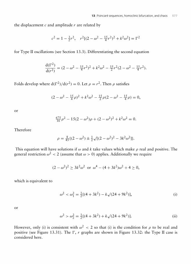
13 : Poincaré sequences, homoclinic bifurcation, and chaos 577
the displacement c and amplitude r are related by
c2 = 1− 32r
2, r2[(2− ω2 − 154 r
2)2 + k2ω2] = 2
for Type II oscillations (see Section 13.3). Differentiating the second equation
d(2)
d(r2)= (2− ω2 − 15
4 r2)2 + k2ω2 − 15
2 r2(2− ω2 − 15
4 r2).
Folds develop where d(2)/d(r2) = 0. Let ρ = r2. Then ρ satisfies
(2− ω2 − 154 ρ)
2 + k2ω2 − 152 ρ(2− ω2 − 15
4 ρ) = 0,
or
67516 ρ
2 − 15(2− ω2)ρ + (2− ω2)2 + k2ω2 = 0.
Therefore
ρ = 845 (2− ω2)± 1
2√[(2− ω2)2 − 3k2ω2].
This equation will have solutions if ω and k take values which make ρ real and positive. Thegeneral restriction ω2 < 2 (assume that ω > 0) applies. Additionally we require
(2− ω2)2 ≥ 3k2ω2 or ω4 − (4+ 3k2)ω2 + 4 ≥ 0,
which is equivalent to
ω2 < ω21 = 1
2 [(4+ 3k2)− k√(24+ 9k2)], (i)
or
ω2 > ω22 = 1
2 [(4+ 3k2)+ k√(24+ 9k2)]. (ii)
However, only (i) is consistent with ω2 < 2 so that (i) is the condition for ρ to be real andpositive (see Figure 13.31). The , r graphs are shown in Figure 13.32: the Type II case isconsidered here.

578 Nonlinear ordinary differential equations: problems and solutions
0.2 0.4 0.6 0.8 1k
1
2
3
4
5
6
v
v2
v 22
12
Figure 13.31 Problem 13.35: Graph shows ω2 = ω21, ω2 = ω2
2 and ω2 = 2, all plotted against k: ρ is real andpositive in the shaded region.
1
1
2r
Type I
Type II
Figure 13.32 Problem 13.35:
• 13.36 It was shown in NODE, Section 13.5 for the Duffing equation x + kx − x +x3 = cosωt that the perturbation a′ = [a′, b′, c′, d ′]T from the translation c0 =√[1− 3
2 (a20 + b2
0)] and the amplitudes a0 and b0 of the harmonic approximation x =c0 + a0 cosωt + b0 sinωt satisfies a′ = Aa′ where
A =
R(P − 32 ka
20 + 3a0b0ω) −R(Q− 3
2 ka0b0 + 3b20ω) 6Rc0(−a0k + 2b0ω) 0
R(Q− 3a20ω − 3
2 ka0b0) R(P − 3a0b0ω − 32b
20k) −12Ra0c0k 0
0 0 0 1
−3a0c0 −3b0c0 −(2− 3r20 ) −k
,
where R = 1/(k2 + 4ω2), P = −k(2 + ω2 − 154 r
20 ), Q = ω(4 − 2ω2 − k2 − 15
4 r20 ), (see
eqn (13.37) in NODE). The constants a0 and b0 are obtained by solving eqns (13.21) and(13.22). Devise a computer program to find the eigenvalues of the matrix A for k = 0.3and ω = 1.2 as in the main text. By tuning the forcing amplitude , find, approximately,the value of for which one of the eigenvalues changes sign so that the linear system

13 : Poincaré sequences, homoclinic bifurcation, and chaos 579
a′ = Aa′ becomes unstable. Investigate numerically how this critical value of varies withthe parameters k and ω.
13.36. In the Duffing equation
x + kx − x + x3 = cosωt ,
let a = a0+a′(t), b = b0+b′(t), c = c0+ c′(t), d = d ′(t). As in the text, it follows that a′ = Aa′where
A =
R(P − 32 ka
20 + 3a0b0ω) −R(Q− 3
2 ka0b0 + 3b20ω) 6Rc0(−a0k + 2b0ω) 0
R(Q− 3a20ω − 3
2 ka0b0) R(P − 3a0b0ω − 32b
20k) −12Ra0c0k 0
0 0 0 1
−3a0c0 −3b0c0 −(2− 3r20 ) −k
,
where
R = 1k2 + 4ω2 , P = −k(2+ ω2 − 15
4 r20 ), Q = ω(4− 2ω2 − k2 − 15
4 r20 ).
The amplitudes a0 and b0, and c0 satisfy (13.20), (13.21) and (13.22), namely
c20 = 1− 3
2r20 , (i)
a0(2− ω2 − 154 r
20 )+ kωb0 = , (ii)
b0(2− ω2 − 154 r
20 )− kωa0 = 0. (iii)
The procedure is that eqns (i), (ii) and (iii) are solved numerically for a0, b0 and c0 for givenvalues of the parameters k, ω and . Then the eigenvalues of A are computed which will thenindicate whether the solutions of a′ = Aa′ are stable or unstable. A table of eigenvalues fork = 0.3, ω = 1.2 and = 0.2, 0.25, 0.3, 0.35 is shown below which can be compared with thecomputed value of = 0.27 (see NODE, Section 13.3).
eigenvalues of A
0.20 −0.202± 1.276i, −0.117 ± 0.350i0.25 −0.249± 1.149i, −0.054±−0.2630.30 −0.171± 0.930i, −0.224, 0.0520.35 −0.408± 1.192i, 0.072± 0.568i
For = 0.2, 0.25, the first harmonic x = c0+ a0 cosωt + b0 sinωt is stable. Instability arisesat approximately = 0.3.

580 Nonlinear ordinary differential equations: problems and solutions
z
x
y
150
6060
Figure 13.33 Problem 13.37: Periodic solution of the Lorenz system with a = 10, b = 100.5, c = 8/3.
t
x
t
x
Figure 13.34 Problem 13.37: Time solutions for a = 10, c = 8/3 with b = 166 in the upper figure and b = 166.1in the lower figure.
• 13.37 Compute solutions for the Lorenz system
x = a(y − x), y = bx − y − xz, z = xy − cz,for the parameter section a = 10, c = 8/3 and various values of b: this is the sectionfrequently chosen to illustrate oscillatory features of the Lorenz attractor. In particu-lar try b = 100.5 and show numerically that there is a periodic attractor as shown inFigure 13.46(a) (in NODE). Why will this limit cycle be one of a pair?Shows also that at b = 166, the system has a periodic solution as shown in Figure 13.46(b)(inNODE), but at 166.1 (Figure 13.46(c) in NODE) the periodic solution is regular for longperiods but is then subject to irregular bursts at irregular intervals before resuming its oscil-lation again. This type of chaos is known as intermittency. (For discussion of intermittentchaos and references see Nayfeh and Balachandran (1995); for a detailed discussion of theLorenz system see Sparrow (1982)).
13.37. The Lorenz system is
x = a(y − x), y = bx − y − xz, z = xy − cz.

13 : Poincaré sequences, homoclinic bifurcation, and chaos 581
A computed periodic solution is shown in Figure 13.33 with the parameters a = 10, b = 100.5,c = 8/3. Time solutions showing intermittency for a small change in the parameter b aredisplayed in Figure 13.34.
• 13.38 The damped pendulum with periodic forcing of the pivot leads to the equation(Bogoliubov and Mitropolski 1961)
x + sin x = ε(γ sin t sin x − κx),where 0 < ε 1. Apply Melnikov’s method and show that heteroclinic bifurcation occursif γ ≥ 4κ sinh 1
2π . [You will need the integral∫ ∞
−∞sin s sech 2
s tanh sds = π
2 sinh(12aπ)
.
]
13.38. The damped pendulum with periodic forcing of the pivot leads to the equation
x + sin x = ε(γ sin t sin x − κx),
where it is assumed that 0 < ε 1. This system has equilibrium points at x = nπ , (n =0,±1,±2, . . . ). Of these points, those for which n = 0,±2,±4, . . . are saddle points, andthose for which n = ±1,±3, . . . are centres.
The heteroclinic paths for the unperturbed system with ε = 0 are given
x0 = 2 tan−1(sinh t).
The Melnikov function (see NODE, Section 13.7) is given by
M(t0) =∫ ∞
−∞y0(t − t0)h[x0(t − t0), y0(t − t0), t]dt ,
where x = y and h(x, y, t) = γ sin t sin x − κy). Therefore
M(t0) = 2∫ ∞
−∞sech (t − t0)γ sin t sin[2 tan−1(sinh(t − t0))] − 2κsech (t − t0)dt
= 4∫ ∞
−∞sech (t − t0)[γ sin tsech (t − t0) tanh(t − t0)− κsech (t − t0)]dt

582 Nonlinear ordinary differential equations: problems and solutions
= 4γ∫ ∞
−∞sin(s + t0)sech 2
s tanh sds − 4κ∫ ∞
−∞sech 2
sds
= 4γ cos t0
∫ ∞
−∞sin s sech 2
s tanh sds − 4κ∫ ∞
−∞sech 2
sds
= 2γ cos t0sinh 1
2π− 8κ,
since ∫ ∞
−∞sech 2
sds = 2,∫ ∞
−∞sin s sech 2
s tanh sds = π
2 sinh(12π)
.
A heteroclinic bifurcation occurs if M(t0) = 0, that is, if
γ cos t0 = 4κ sinh(12π).
A solution for t0 can only exist if4κ sinh(1
2π) ≤ γ ,
assuming that the parameters are positive.
• 13.39 An alternative method of visualizing the structure of solutions of difference equa-tions and differential equations is to plot return maps of un−1 versus un. For example, asequence of solutions of the logistic difference equation un+1 = αun(1 − un) the ordinatewould be un−1 and the abscissa un. The return map should be plotted after any initial tran-sient returns have died out. If α = 2.8 (see Section 13.4), how will the long-term returnamp appear? Find the return map for α = 3.4 also. An exact (chaotic) solution of thelogistic equation is un = sin2(2n) (see NODE, Problem 13.14). Plot the points (un, un−1)
for n = 1, 2, . . . , 200, say. What structure is revealed?Using a computer program generate a time-series (numerical solution) for the Duffingequation
x + kx − x + x3 = cosωt
for k=0.3, ω=1.2 and selected values of , say =0.2, 0.28, 0.29, 0.37, 0.5 (seeFigures 13.14, 13.15, 13.16 in NODE). Plot transient-free return maps for the interpolatedpairs [x(2πn/ω), x(2π(n−1)/ω)]. For the chaotic case =0.5, take the time series over aninterval 0 ≤ t ≤ 5000, say. These return diagrams show that structure is recognizable inchaotic outputs: the returns are not uniformly distributed.
13.39. In this problem return maps are constructed. For the difference equation
un+1 = αun(1− un),
a sequence of solutions are plotted on the (un−1, un) plane.
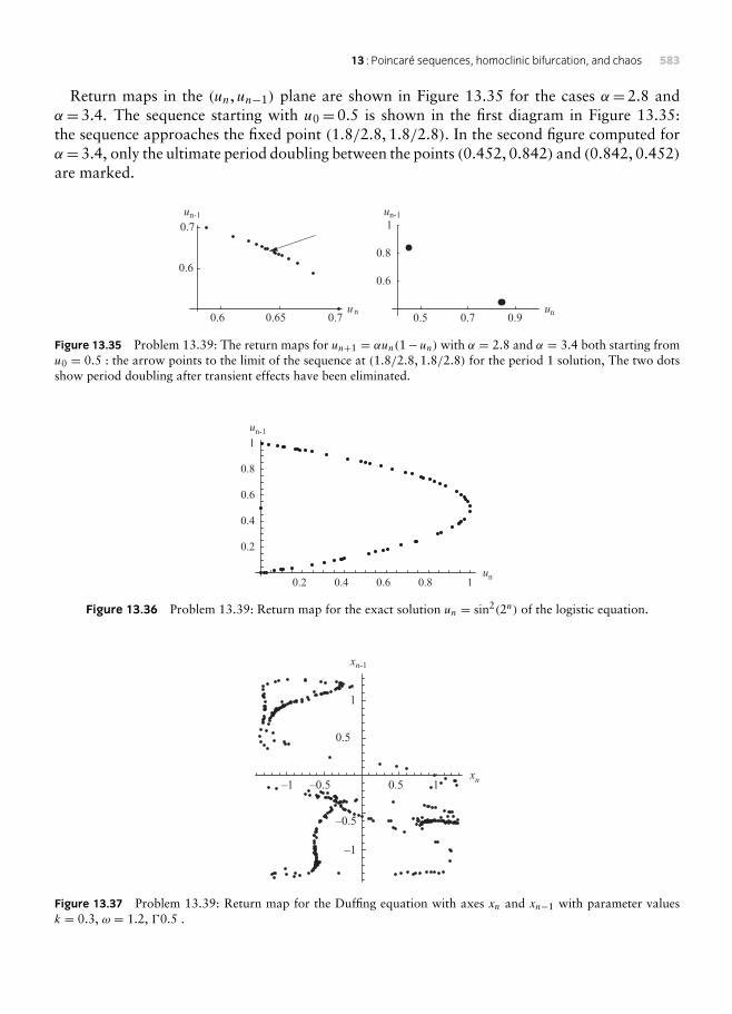
13 : Poincaré sequences, homoclinic bifurcation, and chaos 583
Return maps in the (un, un−1) plane are shown in Figure 13.35 for the cases α=2.8 andα=3.4. The sequence starting with u0=0.5 is shown in the first diagram in Figure 13.35:the sequence approaches the fixed point (1.8/2.8, 1.8/2.8). In the second figure computed forα=3.4, only the ultimate period doubling between the points (0.452, 0.842) and (0.842, 0.452)are marked.
0.6 0.65 0.7un
0.6
0.7un-1
0.5 0.7 0.9un
0.6
0.8
1un-1
Figure 13.35 Problem 13.39: The return maps for un+1 = αun(1−un) with α = 2.8 and α = 3.4 both starting fromu0 = 0.5 : the arrow points to the limit of the sequence at (1.8/2.8, 1.8/2.8) for the period 1 solution, The two dotsshow period doubling after transient effects have been eliminated.
0.2 0.4 0.6 0.8 1un
0.2
0.4
0.6
0.8
1
un-1
Figure 13.36 Problem 13.39: Return map for the exact solution un = sin2(2n) of the logistic equation.
–1 –0.5 0.5 1xn
–1
–0.5
0.5
1
xn-1
Figure 13.37 Problem 13.39: Return map for the Duffing equation with axes xn and xn−1 with parameter valuesk = 0.3, ω = 1.2, 0.5 .

584 Nonlinear ordinary differential equations: problems and solutions
The logistic equation has the exact solution un= sin2(2n) (see Problem 13.14). The chaoticreturn map for this solution is shown in Figure 13.36. Since un=4un−1(1−un−1), all the pointson the return map lie on the parabola x=4y(1− y) in continuous variables.
The Duffing equation is
x + kx − x + x3 = cosωt , x = y.
We shall only look at the case k = 0.3, ω = 1.2, = 0.5, and in particular the returnmap. This is obtained by computing the solution numerically, and then listing the discretevalues xn = x(2nπ/ω) for n = n0, n0 + 1, . . . , where n0 is some suitable value which reducestransience. The return map is shown in Figure 13.36 for about 1000 returns. It can be seen thatthere is structure in the chaos: the returns are not simply randomly distributed over a region.

References
This is the list of references given in Nonlinear Ordinary Differential Equations.
Abarnarnel DI, Rabinovich MI and Sushchik MM (1993) Introduction to nonlinear dynamicsfor physicists. World Scientific, Singapore.
Abramowitz M and Stegun IA (1965) Handbook of mathematical functions. Dover, London.Acheson D (1997) From calculus to chaos. Oxford University Press.Addison PS (1997) Fractals and chaos: an illustrated course. Institute of Physics, Bristol.Ames WF (1968) Nonlinear equations in transport processes. Academic Press, New York.Andronov AA and Chaikin CE (1949) Theory of oscillations. Princeton University Press.Andronov AA, Leontovich EA, Gordon II and Maier AG (1973a) Qualitative theory of second-
order dynamic systems. Wiley, New York.Andronov AA, Leontovich EA, Gordon II and Maier AG (1973b) Theory of bifurcations of
dynamic systems in a plane. Halstead Press, New York.Arnold VI (1983) Geometrical methods in the theory of ordinary differential equations.
Springer-Verlag, Berlin.Arrowsmith DK and Place CM (1990). An introduction to dynamical systems. Cambridge
University Press.Ayres F (1962) Matrices. Schaum, New York.Baker GL and Blackburn JA (2005) The Pendulum. Oxford University Press.Barbashin EA (1970) Introduction to the theory of stability. Wolters-Noordhoff, The
Netherlands.Bogoliubov NN and Mitropolsky YA (1961) Asymptotic methods in the theory of oscillations.
Hindustan Publishing Company, Delhi.Boyce WE and DiPrima RC (1996) Elementary differential equations and boundary-value
problems. Wiley, New York.Brown R and Chua LO (1996) Clarifying chaos examples and counterexamples. Int.
J. Bifurcation Chaos, 6, 219–249.Brown R and Chua LO (1998) Clarifying chaos II: Bernoulli chaos, zero Lyapunov exponents
and strange attractors. Int. J. Bifurcation Chaos. 8, 1–32.Carr J (1981) Applications of center manifold theory. Springer-Verlag, New York.Cesari L (1971)Asymptotic behaviour and stability problems in ordinary differential equations.
Springer, Berlin.Coddington EA and Levinson L (1955) Theory of ordinary differential equations. McGraw-
Hill, New York.Cohen AM (1973) Numerical analysis. McGraw-Hill, London.Coppel WA (1978) Dichotomies in stability thoery. Springer, Berlin.Copson ET (1965) Asymptotic expansions. Cambridge University Press.

586 References
Crocco L (1972) Coordinate perturbations and multiple scales in gas dynamics. Phil. Trans.Roy. Soc. A272, 275–301.
Diacu F and Holmes P (1996) Celestial encounters. Princeton University Press.Drazin PG (1992) Nonlinear systems. Cambridge University Press.Ermentrout B (2002) Simulating, analyzing, and animating dynamical systems: a guide to
XPPAUT. SIAM Publications, Philadelphia.Ferrar WL (1950) Higher algebra. Clarendon Press, Oxford.Ferrar WL (1951) Finite matrices. Clarendon Press, Oxford.Gradshteyn IS and Ryzhik (1994) Table of integrals, series, and products. Academic Press,
London.Grimshaw R (1990) Nonlinear ordinary differential equations. Blackwell Scientific Publica-
tions, Oxford.Guckenheimer J and Holmes P (1983) Nonlinear oscillations, dynamical systems, and
bifurcations of vector fields. Springer-Verlag, New York.Hale J (1969) Ordinary differential equations. Wiley-Interscience, London.Hale J and Kocak H (1991) Dynamics and bifurcations. Springer-Verlag, New York.Hayashi C (1964) Nonlinear oscillations in physical systems. McGraw-Hill, New York.Hilborn RC (1994) Chaos and nonlinear dynamics. Oxford University Press.Hill R (1964) Principles of dynamics. Pergamon Press, Oxford.Hinch EJ (1991) Perturbation methods, Cambridge University Press.Holmes P (1979) A nonlinear oscillator with a strange attractor. Phil. Trans. Roy. Soc. A292,
419–448.Jackson EA (1991) Perspectives in nonlinear dynamics, Vols 1 and 2. Cambridge University
Press.Jones DS (1963) Electrical and mechanical oscillations. Routledge and Kegan Paul, London.Jordan DW and Smith P (2002) Mathematical techniques, 3rd edn. Oxford University Press.Kevorkian J and Cole JD (1996) Multiple scale and singular perturbation methods. Springer,
New York.Krylov N and Bogoliubov N (1949) Introduction to nonlinear mechanics. Princeton University
Press.La Salle and Lefshetz S (1961) Stability of Liapunov’s direct method. Academic Press,
New York.Leipholz H (1970) Stability theory. Academic Press, New York.Logan JD (1994) Nonlinear partial differential equations. Wiley-Interscience, New York.Lorenz EN (1963) Deterministic nonperiodic flow. J. Atmospheric Sci. 20, 130–141.Magnus K (1965) Vibrations. Blackie, London.Mattheij RMM and Molenaar J (1996) Ordinary differential equations in theory and practice.
Wiley, Chichester.McLachlan NW (1956) Ordinary differential equations in engineering and physical sciences.
Clarendon Press, Oxford.Minorsky N (1962) Nonlinear oscillations. Van Nostrand, New York.Moon FC (1987) Chaotic vibrations. Wiley, New York.Nayfeh AH (1973) Perturbation methods. Wiley, New York.Nayfeh AH and Balachandran B (1995) Applied nonlinear dynamics. Wiley, New York.Nayfeh AH and Mook DT (1979) Nonlinear oscillations. Wiley, New York.

References 587
Nemytskii VV and Stepanov VV (1960) Qualitative theory of differential equations. PrincetonUniversity Press.
Nicolis G (1995) Introduction to nonlinear science. Cambridge University Press.O’Malley RE (1974) Introduction to singular perturbations. Academic Press, New York.Osborne AD (1998) Complex variables and their applications. Addison-Wesley Longman.Pavlidis T (1973) Biological oscillators: their mathematical analysis. Academic Press,
New York.Pielou EC (1969) An introduction to mathematical ecology. Cambridge University Press.Poston T and Stewart I (1978) Catastrophe theory and its applications. Pitman, London.Rade L and Westergren B (1995) Mathematics handbook for science and engineering.
Studentlitteratur, Lund, Sweden.Rasband SN (1990) Chaotic dynamics of nonlinear systems. Wiley, New York.Reissig R, Sansone G and Conti R (1974) Nonlinear differential equations of higher order.
Noordhoff, Leiden.Rosen R (ed) (1973) Foundations of mathematical systems, Volume III, Supercellular systems.
Academic Press, New York.Sanchez DA (1968) Ordinary differential equations and stability theory. Freeman, San
Francisco.Simmonds JG (1986) A first look at perturbation theory. Krieger publishing, Florida.Small RD (1989) Population growth in a closed system. In Mathemtical modelling; classroom
notes in applied mathematics, edited by MS Klamkin. SIAM Publications, Philadelphia.Sparrow C (1982) The Lorenz equations: bifurcations, chaos, and strange attractors. Springer-
Verlag, New York.Stoker JJ (1950) Nonlinear vibrations. Interscience, New York.Strogatz SH (1994) Nonlinear dynamics and chaos. Perseus, Massachusetts.Struble RA (1962) Nonlinear differential equations. McGraw-Hill, New York.Thompson JMT and Stewart HB (1986) Nonlinear dynamics and chaos. Wiley, Chichester.Ueda Y (1980) Steady motions exhibited by Duffing’s equation: a picture book of regular
and chaotic motions. In New approaches to nonlinear problems in dynamics, edited by PJHolmes. SIAM Publications, Philadelphia.
Urabe M (1967) Nonlinear autonomous oscillations. Academic Press, New York.Van Dyke, M (1964) Perturbation methods in fluid mechanics. Academic Press, New York.Verhulst F (1996) Nonlinear differential equations and dynamical systems, 2nd edn. Springer,
Berlin.Virgin LN (2000) Introduction to experimental nonlinear dynamics. Cambridge University
Press.Watson GN (1966) A treatise on theory of Bessel functions. Cambridge University Press.Whittaker ET and Watson GN (1962) A course of modern analysis. Cambridge University
Press.Wiggins S (1990) Introduction to applied nonlinear dynamical systems and chaos. Springer-
Verlag, New York.Wiggins S (1992) Chaotic transport in dynamical systems. Springer-Verlag, New York.Willems S (1992) Stability theory of dynamical systems. Nelson, London.Wilson HK (1971) Ordinary differential equations. Addison-Wesley, Reading, MA.Wolfram S (1996) The Mathematica book. Cambridge University Press.


![I mlhlhhEElhhlhI NONEhmhmhhml El.'lllllthe nonlinear Klein-Gordon equation. This extended Kuzmak's work [2] on oscillatory solutions of nonlinear ordinary differential equations to](https://img.dokumen.tips/doc/110x75/6022d50d5a7e26459d730d74/i-mlhlhheelhhlhi-nonehmhmhhml-ellllll-the-nonlinear-klein-gordon-equation-this.jpg)