Embed Size (px)
Citation preview

Model Identification and Data Analysis (Academic year 2014-2015)
Prof. Sergio Bittanti
Laboratory lecture 12/12/2014
Prof. Marcello Farina
TexPoint fonts used in EMF. Read the TexPoint manual before you delete this box.: AAAAAAA

Outline • Time series and systems
– Definition and generation of time series and dynamic systems – Analysis of systems – Analysis of time series (sampled covariance and spectral analysis)
• Optimal predictors
• Identification
– Parameter identification – Structure selection – Model validation
• Exercizes
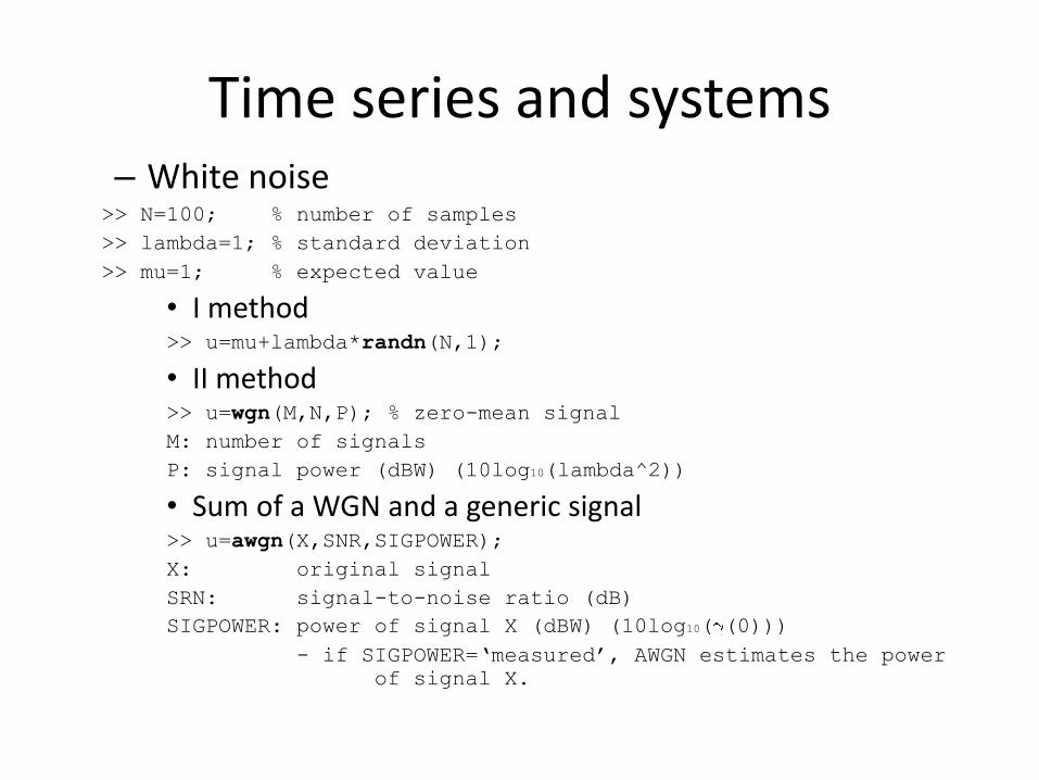
Time series and systems – White noise
>> N=100; % number of samples
>> lambda=1; % standard deviation
>> mu=1; % expected value
• I method >> u=mu+lambda*randn(N,1);
• II method >> u=wgn(M,N,P); % zero-mean signal
M: number of signals
P: signal power (dBW) (10log10(lambda^2))
• Sum of a WGN and a generic signal >> u=awgn(X,SNR,SIGPOWER);
X: original signal
SRN: signal-to-noise ratio (dB)
SIGPOWER: power of signal X (dBW) (10log10( (0)))
- if SIGPOWER=‘measured’, AWGN estimates the power
of signal X.

Time series and systems
• Definition of dynamic linear discrete-time systems: external representation (transfer function – LTI format)
>> system = tf(num,den,Ts)
– num: numerator
– den: denominator
– Ts: sampling time (-1 default)
>> system=tf([1 1],[1 -0.8],1)
Transfer function:
z + 1
-------
z - 0.8

Time series and systems
• Step response of a LTI system >> T=[0:Ts:Tfinal];
>> [y,T]=step(system,Tfinal); % step response
>> step(system,Tfinal) % plot
• Response of a LTI system to a general input signal >> T=[0:Ts:Tfinal];
>> u1=sin(0.1*T); % e.g., sinusoidal input
>> u2=1+randn(T,1); % e.g., white gaussian noise
>> [y,T]=lsim(system,u1+u2,T);
Time series and systems
The SYSTEM IDENTIFICATION TOOLBOX uses different formats for models (detto IDPOLY format) and signals (detto IDDATA format)
Definition of IDDATA objects: >> yu_id=iddata(y,u,Ts);
u: input data
y: output data
Ts: sampling time
Time series and systems – Definition of IDPOLY objects:
>> model_idpoly = idpoly(A,B,C,D,F,NoiseVariance,Ts)
A,B,C,D,F are vectors (i.e., containing coefficients of the
polynomials in incresing order of the exponent of z-1)
Model_idpoly:
A(q) y(t) = [B(q)/F(q)] u(t-nk) + [C(q)/D(q)] e(t)
(If ARMAX: F=[], D=[])
The delay nk is defined in polynomial nk.
>> conversion from LTI format:
Model_idpoly = idpoly(model_LTI)
model_LTI is a LTI model (defined, e.g., using tf, zpk, ss)
– Response of an IDPOLY system to a generic input signal (vector u)
>> y=sim(model_idpoly,u);

Time series and systems
• Analysis of systems (both for LTI and IDPOLY formats): – Zeri e poli: >> [Z,P,K]=zpkdata(model)
Z = [-1] % positions of the zeros
P = [0.8000] % positions of the poles
K = 1 transfer constant
– Bode diagrams: >> [A,phi] = bode(model,W)
W: values of the angular frequency ‘w’ where to compute ‘A(w)’
and ‘phi(w)’
A: amplitude (A(w))
Phi: phase (phi(w))
Time series and systems
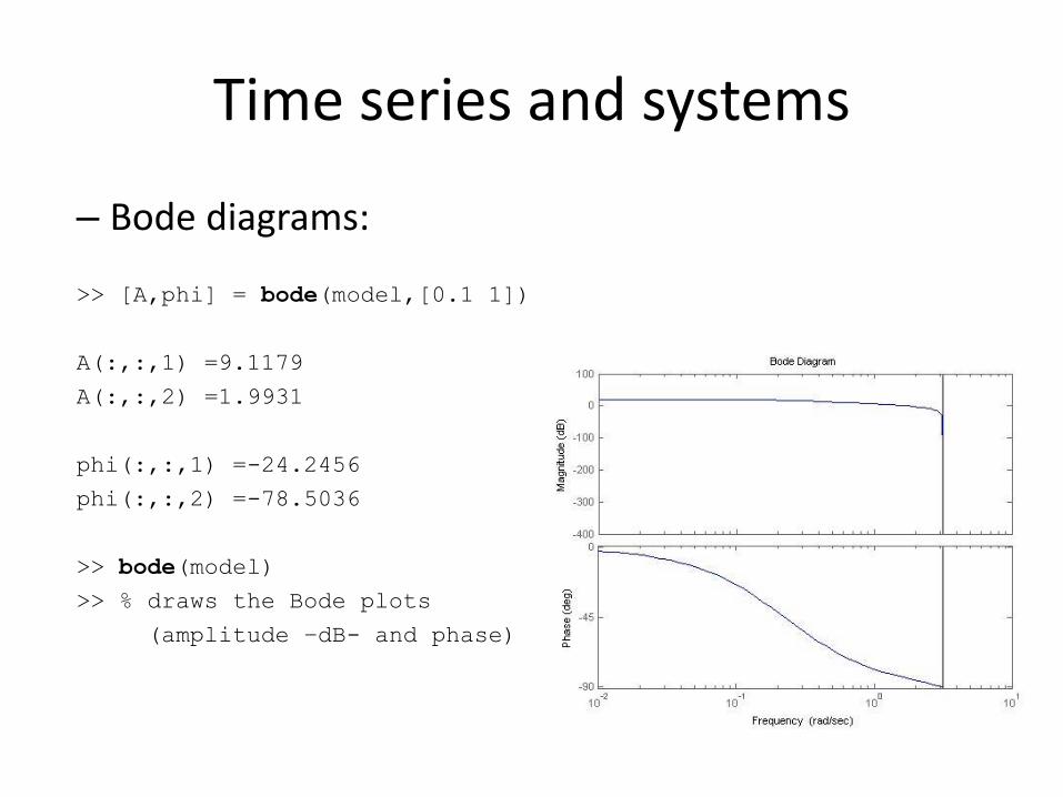
– Bode diagrams:
>> [A,phi] = bode(model,[0.1 1])
A(:,:,1) =9.1179
A(:,:,2) =1.9931
phi(:,:,1) =-24.2456
phi(:,:,2) =-78.5036
>> bode(model)
>> % draws the Bode plots
(amplitude –dB- and phase)
Time series and systems
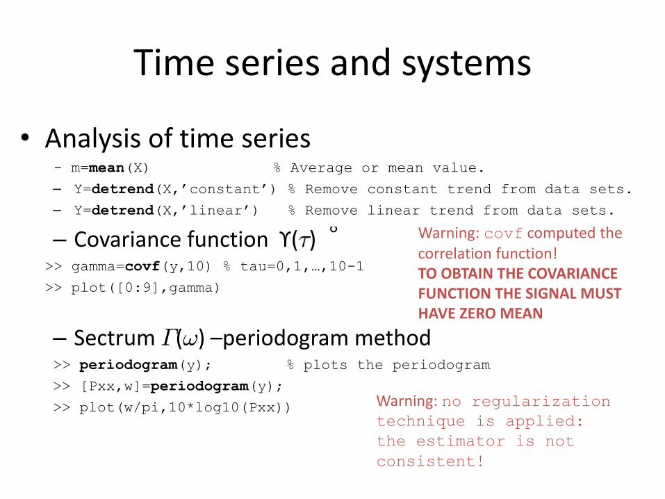
• Analysis of time series - m=mean(X) % Average or mean value.
– Y=detrend(X,’constant’) % Remove constant trend from data sets.
– Y=detrend(X,’linear’) % Remove linear trend from data sets.
– Covariance function ϒ(¿) >> gamma=covf(y,10) % tau=0,1,…,10-1
>> plot([0:9],gamma)
– Sectrum ¡(!) –periodogram method >> periodogram(y); % plots the periodogram
>> [Pxx,w]=periodogram(y);
>> plot(w/pi,10*log10(Pxx))
° Warning: covf computed the correlation function! TO OBTAIN THE COVARIANCE FUNCTION THE SIGNAL MUST HAVE ZERO MEAN
Warning: no regularization technique is applied:
the estimator is not
consistent!

Predictors
• Given the system
The optimal k-steps predictor is given by
where Ek(z) e Rk(z) are the result and the remainder, respectively, of the long division, and
𝑅𝑘 𝑧 =𝑅 𝑘 𝑧 𝑧−𝑘
𝑦 𝑡 =𝐵 𝑧
𝐴 𝑧𝑢 𝑡 − 𝑘 +
𝐶 𝑧
𝐴 𝑧𝑒 𝑡 , 𝑒~𝑊𝑁(0, 𝜎2)
𝑦 𝑡|𝑡 − 𝑘 =𝐵(𝑧)𝐸𝑘 𝑧
𝐶 𝑧𝑢 𝑡 − 𝑘 +
𝑅𝑘 𝑧
𝐶 𝑧𝑦 𝑡
=𝐵(𝑧)𝐸𝑘 𝑧
𝐶 𝑧𝑢 𝑡 − 𝑘 +
𝑅 𝑘 𝑧
𝐶 𝑧𝑦 𝑡 − 𝑘

Predictors
C(z)
A(z)
B (z)
A(z)
e(t)
u(t) y(t)
B(z)Ek (z)
C(z)
~Rk (z)
C(z)
SP
+ +
+
+ 𝑧−𝑘 𝑧−𝑘
y(t-k) 𝑦 (t|t-k)

Predictors
- MATLAB function
>> [Yp,X0e,PREDICTOR] = predict(model,yu_id,k) % optimal k-steps
predictor.
inputs model: IDPOLY format
yu_id: IDDATA object
k: # of prediction steps
outputs Yp: IDDATA format
XOe: Initial states
PREDICTOR: IDPOLY format
PREDICTOR{1}: Discrete-time IDPOLY model with two inputs:
- u(t)
- y(t)
Outputs:
A(q) = … -> C(q)
B1(q) = … -> R(q)
B2(q) = … -> E(q)B(q)q^-k
𝑦 𝑡|𝑡 − 𝑘 =𝐵(𝑧)𝐸𝑘 𝑧
𝐶 𝑧𝑢 𝑡 − 𝑘 +
𝑅𝑘 𝑧
𝐶 𝑧𝑦 𝑡

Predictors
- ESEMPIO:
>> modello=idpoly([1 0.3],[0 0 1 0.2],[1 0.5],[],[],1,1)
Discrete-time IDPOLY model: A(q)y(t) = B(q)u(t) + C(q)e(t)
A(q) = 1 + 0.3 q^-1
B(q) = 1 + 0.2 q^-1
C(q) = 1 + 0.5 q^-1
k = 2
>> [yd,xoe,modpred]=predict(modello,dati,2);
>> modpred{1}
Discrete-time IDPOLY model: A(q)y(t) = B(q)u(t) + e(t)
A(q) = 1 + 0.5 q^-1
B1(q) = -0.06 q^-2
B2(q) = q^-2 ( 1 + 0.4 q^-1 + 0.1 q^-2 )

Predictors
– Prediction error
>> Epsilon = pe(model_idpoly,yu_iddata) % k-steps prediction error
– ARDERSON TEST FOR THE PREDICTION ERROR (99% confidence reguion)
>> e=resid(model,data)
inputs model: IDPOLY format
data: IDDATA format (input-output data)
outputs e: IDDATA ([errore di predizione,input])
If the outputs are not specified, a plot is shown:
- Empirical correlation function (empirical - sampled) of the
prediction error
- 99% confidence region
-> if more than 99% of the samples of the normalized
correlation function lie in the confidence region: positive
results of the whiteness Test!

Predictors
• Example:
>> model_idpoly=idpoly([1 0.5],[0 1 0.3],[1 0.6],[],[],1,1)
Discrete-time IDPOLY model: A(q)y(t) = B(q)u(t) + C(q)e(t)
A(q) = 1 + 0.5 q^-1
B(q) = q^-1 + 0.3 q^-2
C(q) = 1 + 0.6 q^-1
This model was not estimated from data.
Sampling interval: 1
>> data=randn(100,2);
>> resid(model_idpoly,data)

Identification >> ident % start the MATLAB identification toolbox GUI
Identification
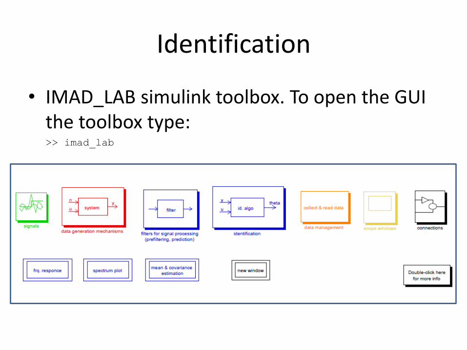
• IMAD_LAB simulink toolbox. To open the GUI the toolbox type:
>> imad_lab

Identification
IMAD_LAB simulink
toolbox (Identification subblock)

Identification Other related Matlab functions (2 Identification toolbox)
• Parametric model estimation – ar - AR-models of signals using various approaches.
– armax - Prediction error estimate of an ARMAX model.
– arx - LS-estimate of ARX-models.
– bj - Prediction error estimate of a Box-Jenkins model.
– ivar - IV-estimates for the AR-part of a scalar time series (with instrumental variable method).
– iv4 - Approximately optimal IV-estimates for ARX-models.
– n4sid - State-space model estimation using a sub-space method.
– nlarx - Prediction error estimate of a nonlinear ARX model.
– nlhw - Prediction error estimate of a Hammerstein-Wiener model.
– oe - Prediction error estimate of an output-error model.
– pem - Prediction error estimate of a general model.
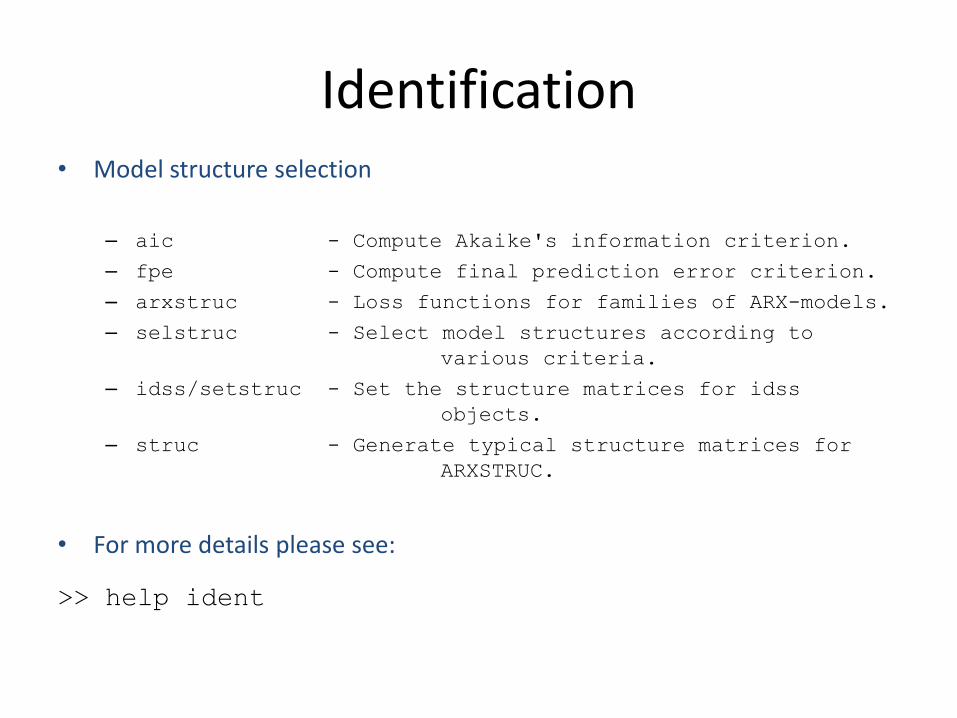
Identification • Model structure selection
– aic - Compute Akaike's information criterion.
– fpe - Compute final prediction error criterion.
– arxstruc - Loss functions for families of ARX-models.
– selstruc - Select model structures according to
various criteria.
– idss/setstruc - Set the structure matrices for idss
objects.
– struc - Generate typical structure matrices for
ARXSTRUC.
• For more details please see:
>> help ident

Exercizes
Linear systems
1. Consider the discrete-time linear system, characterized by the following transfer
function
𝑊 𝑧 =1+𝑧−1
1−0.8𝑧−1
1.1 Plot the step response of the system. What are its features, in the light of the
properties (stability, gain, etc.) of the systems?
1.2 Plot the response of the system to two different sinusoidal inputs, i.e., u(t)=sin(0.1t)
and u(t)=sin(t). Analyze the properties of the two output signals in the light of the
frequency response theorem.
Exercizes
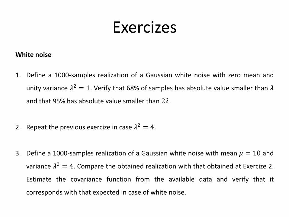
White noise
1. Define a 1000-samples realization of a Gaussian white noise with zero mean and
unity variance 𝜆2 = 1. Verify that 68% of samples has absolute value smaller than 𝜆
and that 95% has absolute value smaller than 2𝜆.
2. Repeat the previous exercize in case 𝜆2 = 4.
3. Define a 1000-samples realization of a Gaussian white noise with mean 𝜇 = 10 and
variance 𝜆2 = 4. Compare the obtained realization with that obtained at Exercize 2.
Estimate the covariance function from the available data and verify that it
corresponds with that expected in case of white noise.

Exercizes
Stationary stochastic processes
1. Consider the stochastic process y(t), generated from the dynamic system
𝑊 𝑧 =1+𝑧−1
1−0.8𝑧−1
with a white noise e(t) as input.
1.1 Assume that e(t) is a white Gaussian noise with mean 𝜇 and variance 𝜆2. Setting
𝜇 = 0 and 𝜆2 = 1, generate different realizations of both e(t) and y(t). Estimate, from
the available data, mean and variance of the processes e(t) and y(t).
1.2 Show the results to the questions below in case 𝜇 = 10 and 𝜆2 = 1. What is the
relationship between the mean of y(t) and the gain of the dynamic system W(z)?
Exercizes
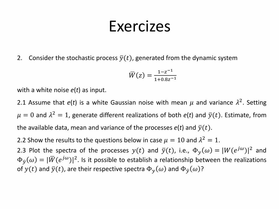
2. Consider the stochastic process 𝑦 (𝑡), generated from the dynamic system
𝑊 𝑧 =1−𝑧−1
1+0.8𝑧−1
with a white noise e(t) as input.
2.1 Assume that e(t) is a white Gaussian noise with mean 𝜇 and variance 𝜆2. Setting
𝜇 = 0 and 𝜆2 = 1, generate different realizations of both e(t) and 𝑦 (𝑡). Estimate, from
the available data, mean and variance of the processes e(t) and 𝑦 (𝑡).
2.2 Show the results to the questions below in case 𝜇 = 10 and 𝜆2 = 1.
2.3 Plot the spectra of the processes 𝑦(𝑡) and 𝑦 (𝑡), i.e., Φ𝑦 𝜔 = |𝑊(𝑒𝑗𝜔)|2 and
Φ𝑦 𝜔 = |𝑊 (𝑒𝑗𝜔)|2. Is it possible to establish a relationship between the realizations
of 𝑦(𝑡) and 𝑦 (𝑡), are their respective spectra Φ𝑦 𝜔 and Φ𝑦 𝜔 ?

Exercizes Predictors
1. Consider the stochastic process y(t), generated from the dynamic system
𝑊 𝑧 =1+0.25𝑧−1
1−0.9𝑧−1
with input e(t), i.e., white Gaussian noise with mean 𝜇 = 0 and variance 𝜆2 = 1.
1.1 Define the optimal 1-step predictor of y(t).
1.2 Define a realization of y(t) and the relative 1-step prediction 𝑦 (𝑡|𝑡 − 1). Compare
the signals y(t) and 𝑦 (𝑡|𝑡 − 1), by drawing them in the same plot.
1.3 Define the signal 𝜀(𝑡) = 𝑦 𝑡 − 𝑦 (𝑡|𝑡 − 1) and plot it. Estimate mean and variance
of 𝜀(𝑡). Compute analytically the theoretical values of the latter quantities and compare
them with those obtaned from data.

Exercizes
1.4 Define now the trivial – non optimal – predictor 𝑦 𝑇 𝑡 𝑡 − 1 = 𝐸 𝑦 𝑡 = 0. Estimate
mean and variance of the estimation error in this case.
1.5 Compare the performances of the predictors defined above.
1.6 Define the optimal 2-step predictor 𝑦 (𝑡|𝑡 − 2) of y(t).
1.7 Define a realization of y(t) and the relative 1-step and 2-step predictions 𝑦 (𝑡|𝑡 − 1)
and 𝑦 (𝑡|𝑡 − 2), respectively. Compare the signals y(t) and 𝑦 (𝑡|𝑡 − 1), and 𝑦 (𝑡|𝑡 − 2), by
drawing them in the same plot.
1.8 Define the signal 𝜀2(𝑡) = 𝑦 𝑡 − 𝑦 (𝑡|𝑡 − 2) and plot it. Estimate mean and variance
of 𝜀2(𝑡). Compute analytically the theoretical values of the latter quantities and compare
them with those obtaned from data.
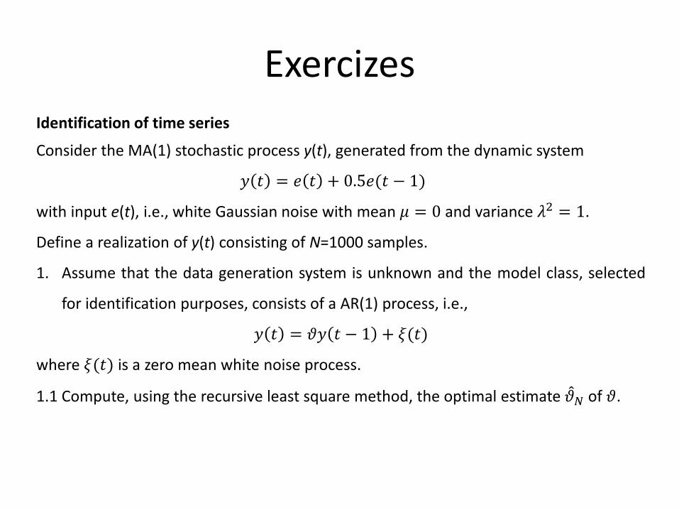
Exercizes Identification of time series
Consider the MA(1) stochastic process y(t), generated from the dynamic system
𝑦 𝑡 = 𝑒 𝑡 + 0.5𝑒(𝑡 − 1)
with input e(t), i.e., white Gaussian noise with mean 𝜇 = 0 and variance 𝜆2 = 1.
Define a realization of y(t) consisting of N=1000 samples.
1. Assume that the data generation system is unknown and the model class, selected
for identification purposes, consists of a AR(1) process, i.e.,
𝑦 𝑡 = 𝜗𝑦 𝑡 − 1 + 𝜉(𝑡)
where 𝜉(𝑡) is a zero mean white noise process.
1.1 Compute, using the recursive least square method, the optimal estimate 𝜗 𝑁 of 𝜗.
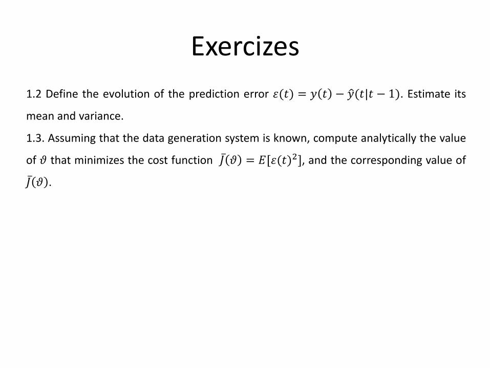
Exercizes
1.2 Define the evolution of the prediction error 𝜀(𝑡) = 𝑦 𝑡 − 𝑦 (𝑡|𝑡 − 1). Estimate its
mean and variance.
1.3. Assuming that the data generation system is known, compute analytically the value
of 𝜗 that minimizes the cost function 𝐽 𝜗 = 𝐸[𝜀(𝑡)2], and the corresponding value of
𝐽 𝜗 .