PRODUCTIVITY MEASUREMENT WITH

CHANGING-WEIGHT INDEXES OF OUTPUTS AND INPUTS

Edwin R. DeanMichael J. HarperMark S. Sherwood

Bureau of Labor StatisticsU.S. Department of Labor

Presented at theOECD Expert Workshop on Productivity:

International Comparison and Measurement IssuesParis, May 2-3, 1996

Revised July 1996and published in

OECD, Industry Productivity:International Comparison and Measurement Issues,

Paris 1996

1

PRODUCTIVITY MEASUREMENT WITH

CHANGING-WEIGHT INDEXES OF OUTPUTS AND INPUTS

This paper examines the use of changing weight indexes of inputs and

outputs in productivity measurement.1 The U.S. Bureau of Labor Statistics (BLS)

productivity measurement program has for many years preferred changing-weight

indexes to fixed-weight indexes. The paper examines the reasons for this

preference and how it has been implemented over time.

The paper examines this broad problem as follows. The next section of

the paper, section 1, discusses weighting schemes for input indexes, from the

viewpoint of the general logic for selecting an input index method and also by

drawing on the theoretical literature relating to input measurement. Section 2

treats output indexes in a parallel fashion. In both sections, it is concluded that

changing-weight indexes are preferable to fixed-weight indexes. The third section

explores several important practical issues that a statistical organization must

resolve before implementing one of the changing-weight index forms and explores

the tension between the ideal methods favored in the theoretical literature and the

practical requirements of an on-going statistical program. This section also

examines the issue of which output concept—for example, value added or gross

output—is appropriate for industries and sectors of the economy. Section 4

describes how BLS has implemented its choice of changing-weight indexes for

productivity data. Section 5 is an analysis of the effects of the BLS changing-

weight indexes on trends in selected input, output, and productivity series. The

final section of this paper, section 6, summarizes the main results of the paper. It

also offers a few observations on international comparisons of productivity trends.

1 We are happy to acknowledge the contributions to this paper made by our colleagues JohnGlaser, Bill Gullickson, Margaret Johnson, Kent Kunze, Phyllis Otto, Larry Rosenblum, andClayton Waring. In addition, Charles Hulten and participants in the May 1996 OECD ExpertWorkshop on Productivity made valuable comments on an earlier draft.

2

1. INPUT INDEXES

In 1983, BLS introduced its first measures of trends in multifactor

productivity (MFP--also referred to frequently as total factor productivity or TFP).

These data were for three major sectors of the U.S. economy, the private business

sector, the private nonfarm business sector and manufacturing; they covered the

years 1948 to 1981. The input measures included were capital services and labor.

An annually-chained Tornqvist index was used both to aggregate detailed capital

services inputs into a single index of total capital input and to aggregate capital and

labor inputs. (The Tornqvist index is a specific changing-weight index which has

been termed a superlative index by several index number theorists; see especially

Diewert (1976).) This work was published in a BLS bulletin (BLS 1983). These

data have been updated, roughly annually, since 1983; to our knowledge this was

the first time that a national statistical office in the United States used a superlative

index in the preparation of an official, periodically published, set of data.

This section discusses the reasons for selecting a changing-weight index,

and specifically the Tornqvist index, for preparing input series for use in

calculating productivity. There is also some discussion of the general merits of a

changing-weight index compared to a fixed-weight index. The section concludes

with a brief discussion of the Fisher Ideal index.

Before discussing the theoretical literature on changing-weight indexes, we

make some introductory comments suggesting that changing-weight indexes have

a strong intuitive appeal. (Later we discuss the foundations of changing-weight

indexes in the index-number literature and in production theory.) Let us compare

a changing-weight index with one type of fixed-weight index. As our example, we

will select an index that makes use of the following fixed-weight method: the

weight for each input is its price, in a base year, or equivalently the weight is each

input’s share of input costs in the base year when the index is constructed by

3

weighting together quantity indexes of individual inputs. These weights are kept

constant over a number of years. Note that constant weights ignore possible

changes in the relative use of inputs that would be expected when relative prices

change. For example, if the price of capital were to increase sharply relative to the

price of labor, enterprises would be likely to begin using relatively more labor

(workers may be hired, shifts increased or hours per shift increased) and relatively

less capital (investment in equipment may be cut back or existing plant or office

space leased to new renters). In this example, two changes take place, as regards

capital: there is an increase in the relative price of capital and a decrease in the

relative quantity of capital. The two changes have opposite effects on the share of

capital in input costs and, as a result, capital’s share could rise, fall, or remain

constant. With base-year share weights, the weight for capital must remain

constant. In this example, fixed weights fail to capture fully the effects of the

input-mix decisions we would expect managers to make. Further, the resulting

input index is dependent on the specific base year selected for the price (or share)

weights. A changing-weight index does not suffer from these problems.

In the literature on productivity measurement, the Tornqvist index is the

changing-weight index that has been most frequently examined and used. The

Tornqvist index, which was developed in the 1930s at the Bank of Finland

(Tornqvist 1936), makes use of logarithms for comparing two entities (e.g., two

countries or two firms) or for comparing a variable pertaining to the same entity at

two points in time. When used to compare inputs for two time periods, in the

context of productivity measurement, it employs an average of cost-share weights

for the two periods being considered. The index number is computed after first

determining a logarithmic change (or rate of proportional change), as follows:

( )ln ln ln lnX X s x xt ti

i i t i t− = ∑ −− −

1 1

4

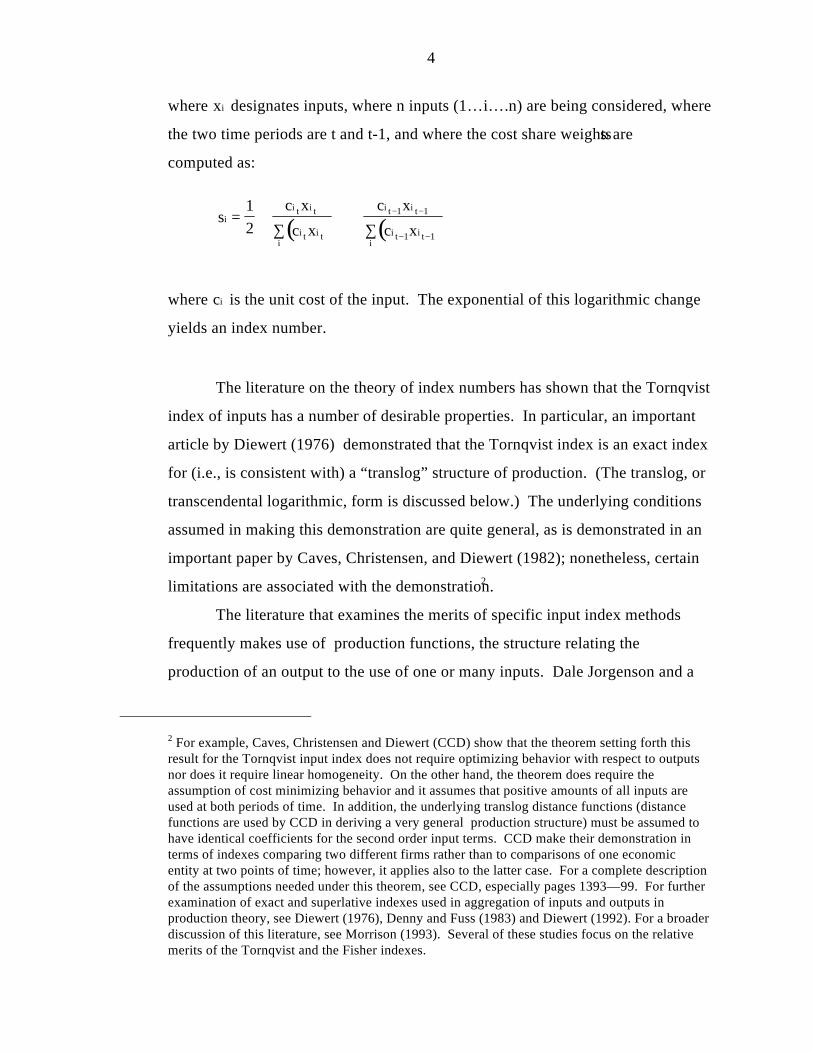
where xi designates inputs, where n inputs (1…i….n) are being considered, where

the two time periods are t and t-1, and where the cost share weightssi are

computed as:

( ) ( )sc x

c x

c x

c xi

i t i t

i t i ti

i t i t

i t i ti

=∑

+

∑

− −

− −

12

1 1

1 1

where ci is the unit cost of the input. The exponential of this logarithmic change

yields an index number.

The literature on the theory of index numbers has shown that the Tornqvist

index of inputs has a number of desirable properties. In particular, an important

article by Diewert (1976) demonstrated that the Tornqvist index is an exact index

for (i.e., is consistent with) a “translog” structure of production. (The translog, or

transcendental logarithmic, form is discussed below.) The underlying conditions

assumed in making this demonstration are quite general, as is demonstrated in an

important paper by Caves, Christensen, and Diewert (1982); nonetheless, certain

limitations are associated with the demonstration.2

The literature that examines the merits of specific input index methods

frequently makes use of production functions, the structure relating the

production of an output to the use of one or many inputs. Dale Jorgenson and a

2 For example, Caves, Christensen and Diewert (CCD) show that the theorem setting forth thisresult for the Tornqvist input index does not require optimizing behavior with respect to outputsnor does it require linear homogeneity. On the other hand, the theorem does require theassumption of cost minimizing behavior and it assumes that positive amounts of all inputs areused at both periods of time. In addition, the underlying translog distance functions (distancefunctions are used by CCD in deriving a very general production structure) must be assumed tohave identical coefficients for the second order input terms. CCD make their demonstration interms of indexes comparing two different firms rather than to comparisons of one economicentity at two points of time; however, it applies also to the latter case. For a complete descriptionof the assumptions needed under this theorem, see CCD, especially pages 1393—99. For furtherexamination of exact and superlative indexes used in aggregation of inputs and outputs inproduction theory, see Diewert (1976), Denny and Fuss (1983) and Diewert (1992). For a broaderdiscussion of this literature, see Morrison (1993). Several of these studies focus on the relativemerits of the Tornqvist and the Fisher indexes.

5

number of collaborators have explored the properties of various production

functions, with a view to determining those most suitable for the study of

productivity and to selecting an appropriate input index method. Jorgenson and

his collaborators have carefully examined and set forth the properties of the

translog production function, which presents output as a transcendental or, more

specifically, exponential function of the logarithms of inputs.3 The merits of the

translog production function include the fact that it places fewer restrictions on

input (and also output) relationships than other functions. It is noteworthy that the

translog function allows the elasticities of substitution among inputs to vary as

input proportions vary, unlike some other production functions including the

Cobb-Douglas function and constant elasticity of substitution functions

(Christensen, Jorgenson, and Lau (1973).)

Tornqvist indexes can be used to combine indexes of broadly-defined

inputs such as capital, labor and purchased intermediate inputs into indexes of total

inputs. They can also appropriately be used for combining detailed inputs—such

as specific types of capital, labor, or intermediate inputs—into aggregate indexes

for each type of input. For example, an aggregate index for capital can be

developed through Tornqvist-aggregation of detailed types of capital inputs. The

productivity literature generally recommends identifying inputs at the finest

3 For example, Gollop and Jorgenson (1980)[G-J], have set forth a very general productionfunction for a sector or an industry, as follows:

( )Z F W,K ,L ,tii

i i i= .

In this formulation , Zi is the output of the sector; Wi , Ki , and Li are inputs of intermediateinputs, capital, and labor respectively; t is time; and i is an index denoting a particular sector.They then proceed to present the translog production function for a sector. See G-J, p. 25. Inempirical work on productivity, it is often assumed that a translog production function ischaracterized by constant returns to scale. For more detailed discussion of this approach ,including a careful justification of the use of the translog in productivity measurement, see forexample G-J, pp. 17-28.

6

possible level of detail and then aggregating, using cost-share weights for each

detailed type, to more broadly-defined inputs, such as total capital or total

intermediate input. The cost share weights are developed using prices, or

estimates of prices, of the detailed inputs.

Several additional comments on input aggregation are appropriate. In the

literature on capital aggregation, a classic article by Hall and Jorgenson (1967) sets

forth the formulae for estimating implicit rental prices of capital. Other

researchers, including Jorgenson, have explained how these rental prices can be

used to aggregate detailed types of capital input for use in measurement of

productivity. A similar approach has been followed in other studies with respect to

labor input (Jorgenson, Gollop, and Fraumeni 1987; Jorgenson and Fraumeni

1989; BLS, 1993, Labor Composition and U.S. Productivity Growth, especially

Appendix A; Dean, Kunze and Rosenblum 1988; Rosenblum et al (1990).)

The literature on input aggregation for productivity measurement purposes

builds on micro-economic theory. It makes use of the concept of the elasticity of

output with respect to inputs and, often, the assumptions of competitive output

and input markets, and in some applications the assumption of constant returns to

scale. While a careful examination of these assumptions is not necessary for

purposes of the present paper, it should be noted that they are critical to the input

aggregation procedures often used, by BLS and by other researchers, and that

these assumptions have been challenged. It should be noted specifically that the

use of cost-share weights for input aggregation generally requires competitive

input markets.4 In addition, the use of implicit rental prices of capital for

estimation of capital service flows is predicated on the additional assumption of

long-run equilibrium in capital goods markets.

7

The Tornqvist index method is not the only index method that could be

used to implement the general idea of calculating indexes for broad input

categories by aggregation from finely-defined inputs. Nor is it the only procedure

that can be used to implement the general preference for changing-weight over

fixed-weight indexes. Other index methods could be used. However, the

Tornqvist index method has been preferred by many researchers in the area of

productivity measurement and analysis, because of the desirable properties

outlined above.

Another frequently-discussed index method for aggregating inputs is the

Fisher Ideal index. The Fisher Ideal quantity index is the geometric mean of the

Laspeyres and Paasche quantity indexes. In productivity studies, the Fisher index

has been used less frequently than the Tornqvist. Some recent work has

emphasized the merits of the Fisher index. In addition, the adoption of the Fisher

index by the BEA for the measurement of real GDP and its main components may

add to the popularity of this index.

Diewert, in his 1992 paper, examined both the Tornqvist and the Fisher

index approaches to input measurement (as well as to output and productivity

measurement). He analyzed the merits of these two indexes from two

perspectives. First, he examined the indexes from the perspective of the “test” or

“axiomatic” approach: which index methods meet a number of tests, or possess

specific mathematical properties, that have been suggested by various writers as

desirable for an input quantity index, or indexes of output and productivity? He

also considers economic approaches to the construction of index numbers of input,

output and productivity. He concludes that there is an equally strong economic

4 It is often necessary to use value-share weights instead of cost-share weights. In that case, it isnecessary to assume competitive output markets as well as input markets and also to assumeconstant returns to scale.

8

justification for Tornqvist and Fisher indexes but that the Tornqvist index does not

pass all the tests passed by the Fisher. We have concluded from this work that

there is no strong reason to prefer one form over the other.

9

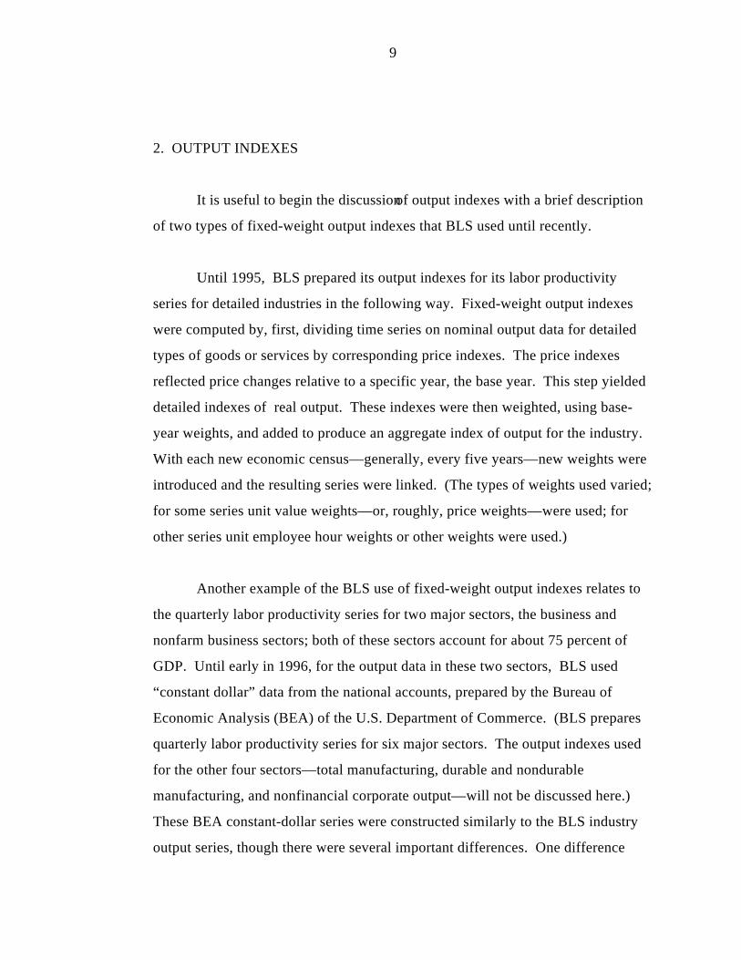
2. OUTPUT INDEXES

It is useful to begin the discussion of output indexes with a brief description

of two types of fixed-weight output indexes that BLS used until recently.

Until 1995, BLS prepared its output indexes for its labor productivity

series for detailed industries in the following way. Fixed-weight output indexes

were computed by, first, dividing time series on nominal output data for detailed

types of goods or services by corresponding price indexes. The price indexes

reflected price changes relative to a specific year, the base year. This step yielded

detailed indexes of real output. These indexes were then weighted, using base-

year weights, and added to produce an aggregate index of output for the industry.

With each new economic census—generally, every five years—new weights were

introduced and the resulting series were linked. (The types of weights used varied;

for some series unit value weights—or, roughly, price weights—were used; for

other series unit employee hour weights or other weights were used.)

Another example of the BLS use of fixed-weight output indexes relates to

the quarterly labor productivity series for two major sectors, the business and

nonfarm business sectors; both of these sectors account for about 75 percent of

GDP. Until early in 1996, for the output data in these two sectors, BLS used

“constant dollar” data from the national accounts, prepared by the Bureau of

Economic Analysis (BEA) of the U.S. Department of Commerce. (BLS prepares

quarterly labor productivity series for six major sectors. The output indexes used

for the other four sectors—total manufacturing, durable and nondurable

manufacturing, and nonfinancial corporate output—will not be discussed here.)

These BEA constant-dollar series were constructed similarly to the BLS industry

output series, though there were several important differences. One difference

10

occurred in the step following the deflation of nominal output data by an

appropriate price index. The constant-dollar data for particular types of goods or

services were directly added to produce constant-dollar output for larger

aggregates. Indexes based on these constant-dollar aggregates effectively

weighted items based on their prices in the base year. Another difference was that

the BEA used the base-year prices of a single year for its entire time series.

However, about every five years BEA selected a new, more recent base year. For

example, in December 1991, as part of new benchmark calculations for its

national accounts data, BEA switched from 1982 price weights for its entire time

series to 1987 price weights.

In 1995, BLS changed its index number method for industry output data

from the procedure described earlier to a changing-weight method. And early in

1996 BEA began to use annually-weighted indexes as its featured series for real

GDP and its major components.5 Before discussing these recent changes, it is

important to discuss the short-comings of fixed-weighted indexes. These problems

are analogous to those discussed above in the section on input indexes.

Fixed-weighted indexes are a reasonably good measure of output if the

prices of various goods are fairly stable relative to one another.6 However, when

relative prices change, fixed-weighted indexes tend to place too much weight on

goods or services for which relative prices have fallen and too little emphasis on

items for which relative prices have risen. This is because “constant dollar” series

and other fixed-weighted series effectively weight items based on their prices in the

5 Both BLS and BEA made some use of annually-weighted output indexes prior to the datesmentioned in this paragraph. BLS first published annually-weighted indexes of output forindustry MFP series in 1987. See Sherwood (1987) and Gullickson and Harper (1987). BEAfirst published annually-weighted data in 1992, as alternative measures of real GDP, whileretaining the constant-dollar series as its featured measure. See BEA (July 1995) and BEA(Jan./Feb. 1996).6 This discussion will not consider the use of unit employee hour weights or other weights usedin some series by BLS in past years; such a discussion is not necessary given the objectives of thispaper.

11

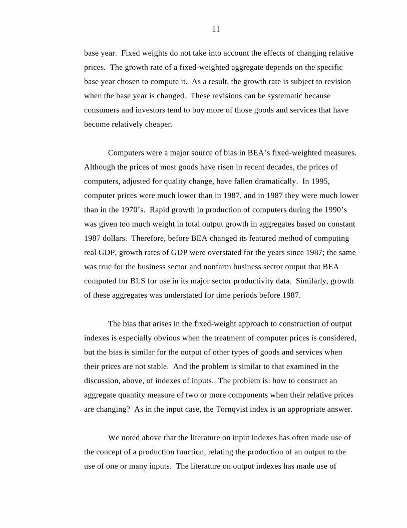
base year. Fixed weights do not take into account the effects of changing relative

prices. The growth rate of a fixed-weighted aggregate depends on the specific

base year chosen to compute it. As a result, the growth rate is subject to revision

when the base year is changed. These revisions can be systematic because

consumers and investors tend to buy more of those goods and services that have

become relatively cheaper.

Computers were a major source of bias in BEA’s fixed-weighted measures.

Although the prices of most goods have risen in recent decades, the prices of

computers, adjusted for quality change, have fallen dramatically. In 1995,

computer prices were much lower than in 1987, and in 1987 they were much lower

than in the 1970’s. Rapid growth in production of computers during the 1990’s

was given too much weight in total output growth in aggregates based on constant

1987 dollars. Therefore, before BEA changed its featured method of computing

real GDP, growth rates of GDP were overstated for the years since 1987; the same

was true for the business sector and nonfarm business sector output that BEA

computed for BLS for use in its major sector productivity data. Similarly, growth

of these aggregates was understated for time periods before 1987.

The bias that arises in the fixed-weight approach to construction of output

indexes is especially obvious when the treatment of computer prices is considered,

but the bias is similar for the output of other types of goods and services when

their prices are not stable. And the problem is similar to that examined in the

discussion, above, of indexes of inputs. The problem is: how to construct an

aggregate quantity measure of two or more components when their relative prices

are changing? As in the input case, the Tornqvist index is an appropriate answer.

We noted above that the literature on input indexes has often made use of

the concept of a production function, relating the production of an output to the

use of one or many inputs. The literature on output indexes has made use of

12

similar concepts, including the production possibility frontier and the

transformation function; these concepts provide a framework for examining the

production of several outputs using several inputs. In particular, production

possibility frontiers and transformation functions allow for the examination of

situations where more than one output is produced.

In the 1973 paper mentioned above, Christensen, Jorgenson, and Lau

explore the characteristics of production possibility frontiers with constant

elasticities of substitution and constant elasticities of transformation. They find

such frontiers unduly restrictive. One of their conclusions, for one class of such

frontiers, is that the frontiers would have proper curvature only with severe

restrictions on the numbers of inputs and outputs that could be considered. In

contrast, the translog production possibility frontier is less restrictive and more

flexible. And Diewert has shown, in the 1976 article mentioned above, that a

Tornqvist output index is exact for a translog production technology. Other

research has demonstrated additional advantageous characteristics of the Tornqvist

output index, analogous to the conclusions regarding input indexes.7

7 See, again, the Caves, Christensen, Diewert (1982) article. As in the input case, the theoremon output indexes set forth in this article requires fewer restrictive assumptions than do someother index formulas. However, some assumptions must be made, as in the input case. In his1992 article, Diewert finds reason to support the Fisher index.

13

3. PROBLEMS OF IMPLEMENTING TORNQVIST AND FISHER

INDEXES

The literature cited and briefly discussed above simply examines indexes for

comparing two economic entities (for example two firms or two countries) at a

point in time or for comparing the same entity at two different points in time.

Usually, we are interested in a larger number of data points, and in particular in

indexes covering entities over a long time span.

This section raises questions that are closer to the practicing statistician’s

practical concerns. First, how should time series—as distinct from comparisons at

two points in time—be constructed? Is a Fisher index preferable to a Tornqvist

index for the construction of time series? Do these two index methods yield

greatly different results? And should the measurement methods for indexes of

inputs, output, and productivity be the same for industries and for larger economic

aggregates, including the total economy?

Time series

The recent literature on index methods, and the closely related literature on

production functions and transformation functions, do offer a major advantage that

some of the earlier literature did not. This recent literature, cited above, is framed

in terms of discrete time units. Some of the earlier literature (Solow (1957),

Jorgenson and Griliches (1967), and Hulten (1973)) showed the relationship

between Divisia indexes and theoretical productivity measures. The Divisia is a

continuous index form; the Tornqvist index is the discrete counterpart of the

Divisia index. As Diewert (1992; p. 211) has pointed out, “Unfortunately, these

Divisia indexes require that price and quantity data . . . be collected on a

continuous time basis, which is impossible empirically”. Some of the recent

14

discussions are specifically framed in terms of indexes that use discrete data.

Among these discussions are several of the contributions discussed above: Diewert

(1976), Gollop and Jorgenson (1980), Caves, Christensen and Diewert (1982),

Diewert (1992). Hence, this literature provides guidance to a statistician who

might seek to use discrete data to compare, for example, the output or

productivity of a firm or an industry at two points in time.

Nonetheless, two-period comparisons are cumbersome for someone who

wishes to understand long-term trends, or developments over the course of one or

several business cycles. It is slightly cumbersome to make a comparison of an

industry’s productivity in 1994 and 1995, another of its productivity in 1995 and

1996, and a third in 1994 and 1996. It is more cumbersome, though still possible,

to add 1997 data to this set of comparisons, thereby adding three more index

numbers (one for 1996 and 1997, another for 1995 and 1997, and a third for 1994

and 1997). Hence, to compare data for any pair of years selected from a four-year

time span requires six index numbers. (In general, the number of comparisons

required is ( ) ( ) ( )12

112

112

2 2n n n n− + − = − .)

It is more convenient to have a single set of consecutive index numbers,

using for example 1994 = 100, and a single index number for each year. In fact, it

is so much more convenient that we seldom consider any other approach. It is

possible to construct such a series by chaining indexes for pairs of consecutive

years. (By “chaining” is meant multiplying indexes together, where each of the

indexes is derived for a two-period comparison.) This can be done for either

Fisher or Tornqvist series. BLS has done this for Tornqvist output indexes and

BEA has done it for Fisher indexes of GDP and its components.

These chained indexes generally yield results that differ from the indexes

produced by pair-wise comparisons. For example, the index for 1996, on the base

15

1994 = 100, that is computed by chaining the indexes for 1995 compared to 1994

and 1996 compared to 1995 will generally differ from the index computed directly

for comparing 1996 and 1994.

Hulten (1973) has examined this issue rigorously for the Divisia index.

Hulten shows that the Divisia index depends, in general, on the specific path

followed by the data between the two time periods being compared. That is, the

index obtained by chaining two Divisia indexes over the years 1994 to 1996 will in

general depend on the observation for 1995. Hulten refers to this as “path

dependence.” And he examines the specific conditions under which this general

conclusion will not hold, that is the conditions under which the Divisia will be

path-independent. Under general conditions, path dependence holds also for

chained Fisher and chained Tornqvist indexes.

Choice of index method

A number of interesting and important attempts have been made to deal

with this problem (for example, Triplett 1988). To examine this body of work

here, however, would lead us beyond our present task. We do need to discuss

briefly, though, two straight-forward practical issues, the choice between chained

and pair-wise comparisons and the choice between the Fisher and Tornqvist

indexes.

In large part, because chained indexes are simpler to prepare and to

understand, the BLS and BEA have chosen to publish chained indexes. For

example, the BLS input indexes, published in 1983 in introducing the BLS

measures of MFP, are annually-chained Tornqvist indexes. In 1992, the BEA first

introduced two new indexes of real GDP and its major components, both based on

the Fisher method, as “alternative” indexes to its constant dollar indexes. One of

these two new indexes was presented in annually-chained form—the “chain-type

16

annual-weighted” index. The other alternative was a Fisher index developed by

computing pair-wise comparisons over a span of years, customarily five-years

apart. For each pair of adjacent benchmark years, two fixed-weighted quantity

indexes were prepared, a Laspeyres and a Paasche index; the geometric mean of

these two indexes, the Fisher index, was titled the “benchmark years-weighted”

index.

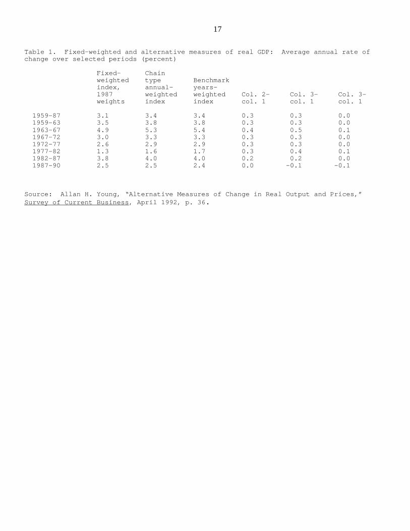
Table 1 shows a comparison of these BEA results, published by BEA in

1992. This table indicates that the two indexes, derived from a chained index

computed from annual pair-wise Fisher indexes, and a pair-wise Fisher computed

over (approximately) five-year spans, yielded very similar results. The differences

between these two indexes in average annual growth rates were never greater than

0.1 percentage point. This result seems to provide a hint that for price and quantity

data that are not especially volatile, the chain-type annual-weighted index and the

pair-wise comparisons over spans of several years may tend to yield similar series.

However, the differences between both of these two indexes and the fixed-weight,

constant-dollar index were substantial, frequently 0.3 of a percentage point or

greater.

17

Table 1. Fixed-weighted and alternative measures of real GDP: Average annual rate ofchange over selected periods (percent)

Fixed- Chainweighted type Benchmarkindex, annual- years-1987 weighted weighted Col. 2- Col. 3- Col. 3-weights index index col. 1 col. 1 col. 1

1959-87 3.1 3.4 3.4 0.3 0.3 0.0 1959-63 3.5 3.8 3.8 0.3 0 3 0.0 1963-67 4.9 5.3 5.4 0.4 0.5 0.1 1967-72 3.0 3.3 3.3 0.3 0.3 0.0 1972-77 2.6 2.9 2.9 0.3 0.3 0.0 1977-82 1.3 1.6 1.7 0.3 0.4 0.1 1982-87 3.8 4.0 4.0 0.2 0.2 0.0 1987-90 2.5 2.5 2.4 0.0 - .1 -0.1

Source: Allan H. Young, “Alternative Measures of Change in Real Output and Prices,”Survey of Current Business, April 1992, p. 36.

18

In January 1996, however, when BEA first published a Fisher-based index

as the “featured” real GDP series, the index selected was the chain-type annual-

weighted Fisher index.

The choice between the Tornqvist and the Fisher index method may also be

made in part on pragmatic grounds. The results obtained by applying the two

methods to the same data are often very similar. Table 2 presents a BLS

comparison of Tornqvist and Fisher indexes of manufacturing sectoral output for

the years 1949-93.8 The two indexes yield nearly identical results. This result is

similar to the results of other, unpublished, calculations made by BLS and to

results presented in the literature that has examined superlative index forms (for

example, see Diewert 1976, especially p. 135).

8 This table is very similar to one published in 1995 (Gullickson 1995), though the earlier tablecompared indexes of manufacturing gross output (rather than sectoral output) and the underlyingdata have since been revised. The revised sectoral output series is presented in BLS, February 8,1996, Appendix Table 3.

19

Table 2. Tornqvist and Fisher Ideal indexes of manufacturingsector output, 1949-93

(1987=100) Year Tornqvist Fisher

1949 28.519 28.527 1950 31.322 31.332 1951 33.408 33.412 1952 35.120 35.120 1953 38.065 38.066 1954 35.642 35.643 1955 39.281 39.283 1956 39.624 39.626 1957 39.789 39.790 1958 37.025 37.025 1959 40.254 40.255 1960 40.764 40.764 1961 40.999 40.999 1962 43.802 43.802 1963 46.055 46.056 1964 49.023 49.024 1965 52.957 52.959 1966 57.101 57.102 1967 59.064 59.063 1968 61.949 61.949 1969 63.557 63.557 1970 61.641 61.641 1971 63.213 63.214 1972 68.496 68.500 1973 74.041 74.043 1974 73.289 73.290 1975 67.930 67.930 1976 74.075 74.077 1977 79.923 79.926 1978 84.348 84.351 1979 85.481 85.481 1980 82.121 82.118 1981 82.758 82.754 1982 79.306 79.301 1983 83.205 83.201 1984 91.153 91.149 1985 93.889 93.884 1986 96.667 96.666 1987 100.000 100.000 1988 104.182 104.182 1989 106.403 106.402 1990 105.946 105.946 1991 104.103 104.102 1992 107.211 107.210 1993 110.967 110.966

Source: Bureau of Labor Statistics, Office of Productivity andTechnology

20

The most important aspect of these new indexes, some analysts have

argued, is the fact that they use changing weights rather than fixed weights, not so

much whether the particular form is Fisher or Tornqvist or whether they are

computed as chained or pair-wise indexes. The choice between the Tornqvist and

Fisher methods and the choice between pair-wise and chained indexes usually

makes little difference, at least for major sectors and large industries in the United

States. (This may be because the underlying data for large sectors and industries in

the U.S. are not especially volatile; these conditions may not hold for detailed

industries.) The important differences, in this view, arise from the choice between

a fixed-weighted and a changing-weight approach.

Productivity indexes for industries and sectors

An additional decision must be taken before output and input indexes can

be implemented as part of a productivity measurement program. A specific output

concept—value added, gross output, or some alternative concept—must be

chosen. The issue of the appropriate output concept for computing the change in

productivity at the level of industries and large sectors of the economy has been

widely examined in the literature. Some analysts have favored a value-added

output concept while others have favored gross output or some other concept

closely allied to gross output.

It seems clear that the literature on industry productivity measurement

unambiguously favors the use of gross output, or a closely related concept, for

multifactor productivity measurement. (As will be seen below, the choice is not so

clear-cut for labor productivity measurement.) This choice of gross output, or a

closely-related concept, is matched on the input side by inclusion of intermediate

inputs along with labor and capital inputs. We need to examine the choice of an

output concept, however, because some researchers have favored a value-added

output concept, accompanied by consideration of labor and capital inputs only.

21

Consider a general production function for an industry or sector, i, in which

the production of gross output is viewed as a function of value added and

intermediate inputs, as follows:

( )[ ]Z f V K L t Wi i i i= , ,

Gross output, Z, is produced by means of a value-added subfunction, V, which

includes technology as well as capital (K) and labor (L), and, in addition, by means

of intermediate inputs, W. This formulation of the production function posits the

separability of value added, the subfunction V, from the overall process of

producing gross output. There are several problems with this formulation. One

problem is the implicit assumption that developments in intermediate inputs, for

example, price change, do not influence the relative use of capital and labor.

Another problem is that this formulation assumes that technological improvements

can affect gross output only through the value-added subfunction. Intermediate

inputs cannot be sources or mediums of productivity growth. In short,

intermediate inputs are excluded from consideration in the value-added model on

the basis of the assumption that they are insignificant to the analysis of productivity

growth.

A number of studies have considered the arguments in favor of computing

multifactor productivity using a value-added output series. Gollop (1983) explores

appropriate models for industry productivity measurement and finds that the use of

value-added output requires quite limiting assumptions. Several studies

considering and rejecting the assumption of value-added separability are discussed

in Gullickson (1995). In this discussion, Gullickson draws on the research results

obtained by Jorgenson, Gollop, and Fraumeni (1987) and Berndt and Wood

(1975).

22

For some time, the BLS has refrained from using value-added output in its

publications on multifactor productivity. Instead, BLS has used “sectoral output,”

a concept closely related to gross output. Sectoral output is the name given to

gross output less intra-sector (or intra-industry) transactions. Sectoral output for

an industry represents deliveries to purchasers outside the industry. For example,

for total manufacturing, sectoral output represents deliveries to purchasers outside

manufacturing.9

The use of value-added output for measurement of labor productivity—as

distinct from its use in MFP measures—has not been closely examined in the

theoretical literature and value-added is in fact frequently used in studies of labor

productivity. A persuasive case can be made for the use of gross or sectoral

output in labor productivity series also. Some of the considerations that underlie

the choice of sectoral or gross output for multifactor productivity measurement

carry over to the area of labor productivity. An appealing insight into this choice

is conveyed by a question inspired by a comment by Domar (1961): who would be

interested in the productivity of producing shoes without leather?

For several decades, the BLS series on labor productivity for selected 3-

and 4-digit industries have been based on gross output (for a number of years

ending in 1995) or the closely-related sectoral output concept (beginning in 1995).

However, until February 1996, the BLS quarterly labor productivity series for total

manufacturing, and the series on durable and nondurable manufacturing, were

based on value-added output. In that month, BLS began using the sectoral output

concept in these series. (For further discussion of these issues, see Dean, Harper,

and Otto (1995) and Kunze, Jablonski, and Klarquist (1995).)

9 For further discussion of the reasons for the choice of sectoral output, see Gullickson (1995),especially the footnotes on p. 27. The removal of intra-sector transactions from output andintermediate input for industry productivity measurement was first suggested by Domar (1961).)

23

A brief comment should be made on the output concept to be used for the

total economy or for sectors comprising most of the economy. BLS does not

publish productivity data for the total economy. However, it does publish data for

the business sector and for the nonfarm business sector, both amounting to about

three-fourths of GDP. The output data, obtained from BEA, for these two sectors

may be viewed as roughly consistent with the value-added concept. And at this

level of aggregation, it seems likely that trends in value added and gross output

data do not differ greatly.

The choice of an appropriate concept to use for international comparisons

of productivity trends is complicated. For MFP comparisons, the sectoral output

concept would appear to be preferable (see Gollop 1983), though BLS has not yet

prepared MFP comparisons using sectoral output.10 For international

comparisons of productivity trends, however, value added data are typically

available. The Bureau of Labor Statistics publishes annual data on international

comparisons of labor productivity for total manufacturing, for the U.S. and 11

other countries (BLS, September 8, 1995). Related series on hourly compensation

and unit labor costs are also published. At the present time, these series make use

of value added output data. Whether value added is the preferred concept for

international comparisons of labor productivity is not clear and it may not be

possible to address it without considering the purposes of the international

comparisons and the particular types of countries to be included in the

comparisons. BLS is presently reviewing the question of the preferred output

concept for international comparisons of labor productivity.

10 It is noted elsewhere in this paper that BLS does publish some MFP comparisons formanufacturing, using value-added output; we are considering the feasibility of developingsectoral output data for MFP comparisons.

24

4. BLS MEASUREMENT PROGRAM: USE OF TORNQVIST AND FISHER

INDEXES

Since 1983, BLS has radically revised its productivity measurement

program. Prior to 1983, the published BLS productivity data made no use of

Fisher or Tornqvist indexes, though the investigation of these methods was

actively under way beginning in the late 1970’s. By 1996, all of the BLS

productivity measures (with the exception of the international comparisons of

trends in manufacturing labor productivity) made extensive use of Tornqvist or

Fisher indexes.

This section summarizes the Bureau’s progress, over the years 1983-96, in

developing new measures based on these index methods. The following section

examines the impact of these new methods on trends in inputs, output, and

productivity.

BLS introduced its first multifactor productivity measures in 1983, as

noted above. These measures covered three sectors--private business, private

nonfarm business and total manufacturing--for the years 1948 to 1981. The inputs

used in this data set were capital services and labor inputs. Tornqvist indexes were

used to aggregate capital services series from information available for detailed

asset categories. The weights used for the aggregation were developed from BLS

estimates of implicit capital rental prices by asset type. This aggregation followed

generally the formulas developed by Hall and Jorgenson (1967) and by Jorgenson

and other colleagues, though BLS (see Harper 1982) adopted an alternative

approach to some components of the rental price formula. Tornqvist indexes were

also used to combine capital services and labor inputs. The output series used

when this set of measures was introduced in 1983 was the BEA fixed-weight

constant-dollar series.

25

In 1987, BLS expanded its use of the Tornqvist method by computing

Tornqvist indexes of outputs as well as improved indexes of inputs. In that year,

two separate studies used Tornqvist indexes, annually-chained, to aggregate inputs

of capital, labor and purchased intermediate inputs, for use in measures of MFP for

industries (Gullickson and Harper 1987; Sherwood 1987). In addition, these two

new sets of measures developed Tornqvist indexes of sectoral output. The choice

of sectoral output, and the inclusion of purchased intermediates among the inputs

was in accord with the conclusions of the literature summarized above. The

Gullickson-Harper study covered 20 two-digit manufacturing industries while the

Sherwood study covered the steel and motor vehicle industries, at the three-digit

level. In the data set covering two-digit manufacturing industries, Tornqvist sub-

aggregates are first developed for energy inputs, purchased inputs of materials, and

purchased business services. These three series are then Tornqvist-aggregated to

the level of total intermediates.

During the late 1980’s, several improvements were made in the capital

measures. BLS began aggregation of capital services by industry detail as well as

by asset detail. Implicit rental prices were estimated at the new, finer, levels of

detail. This step was taken in accord with the conclusion in the literature that

input aggregation should be from the finest possible level of detail and should use

the best possible approximation to marginal revenue product weights. Additional

improvements were made in the rental price formula and applied to the data

(Harper, Berndt, and Wood 1989). To explore the possibilities of further

improvements in capital estimation, studies were made of the possible influence of

increased rates of obsolescence induced by energy price increases (Hulten,

Robertson, and Wykoff 1986) and of alternative data sources for estimation of

capital services (Powers 1988).

26

Prior to 1993, all of the BLS labor input series were simple summations of

hours of labor input, under the assumption that hours of labor were homogeneous.

In 1993, however, Tornqvist indexes of labor composition change were introduced

for the major sector MFP series (BLS, Labor Composition and U.S. Productivity

Growth, 1948-90, 1993; see also Rosenblum et al 1990 and Dean, Kunze and

Rosenblum 1988). In this study, detailed information on the composition of labor

input was developed, with special attention to level of education, gender, and

estimated years of actual work experience (as distinct from the potential work

experience concept). Using wage equations, estimated prices of each type of labor

input were developed. These prices were then used to aggregate the hours of each

type of labor. The approach taken benefited from earlier studies by Jorgenson and

his colleagues (Jorgenson, Gollop and Fraumeni 1987 and Jorgenson and Fraumeni

1989). As in the case of the BLS capital services measure, this approach was

designed to develop an aggregate from the finest possible level of detail, using as

weights the best possible estimates of the marginal revenue product of each input

type.

As of 1994, the BLS productivity program was producing three sets of

multifactor productivity measures—major sector, two-digit manufacturing, and

selected three-and four-digit industries, mainly in manufacturing—and two sets of

labor productivity measures—for major sectors and for detailed industries at the

2-, 3-, and 4-digit levels. In addition, international comparisons of labor

productivity for total manufacturing were published. In 1994, all three of the MFP

data sets used Tornqvist aggregates of inputs, but only the two industry MFP data

sets used a current-weighted index of output. Neither of the two labor

productivity series used current-weighted output indexes, nor did the international

comparisons data set.

During the years 1994 to 1996, current-weighted output indexes were

introduced for all of the BLS productivity data sets for the United States that were

27

not using such indexes. In July 1994, BLS released major sector MFP data

incorporating annually-chained Fisher indexes of output provided by the BEA, in

place of the previously-used BEA constant-dollar series (BLS July 11, 1994).

BLS is grateful to BEA for these series for the private business and private

nonfarm business sectors; BEA computed the data for these two sectors from

elements of their annually-weighted series for GDP.

In July 1995, BLS first published annually-chained Tornqvist indexes of

output for its detailed 3- and 4-digit labor productivity data set. At the same time,

this data set was converted from a gross output to a sectoral output series, by

developing data on intra-industry deliveries and eliminating these deliveries from

gross output (Kunze, Jablonski, and Klarquist, 1995).

In February 1996, current-weighted output data were incorporated into the

quarterly major sector labor productivity series (BLS February 8, 1996). These

output data, also obtained from BEA, are based on data from annually-chained

Fisher indexes.11 This step was taken a few weeks after the BEA adopted a chain-

type annual-weighted series as its featured measure for GDP and its major

components. These BEA data are now used for business, nonfarm business and

nonfinancial corporate output. At the same time, BLS ceased using constant-

dollar value-added series for output in manufacturing and durable and nondurable

manufacturing. It replaced these series with the Tornqvist indexes of sectoral

output developed initially for use in the MFP series for two-digit manufacturing

industries.

With this adoption of these output series for the quarterly labor

productivity data set, all of the BLS data series for the U.S. make use of changing-

weight output series. Regarding inputs, in all of the MFP series the inputs are

11 The historical quarterly data are estimated using prices from the year of the specific quarter forwhich a change is being estimated as well as prices for adjacent years.

28

Tornqvist-aggregated, with the exception of labor input. In all data sets but one,

labor input is a direct aggregate of hours (or, for a few detailed industries,

employees). Only in the major sector MFP series on private business and private

nonfarm business is a Tornqvist index used to estimate the effects on productivity

trends of changes in the composition of the workforce.

Prior to 1995, the only published BLS measures on international

comparisons of productivity were the comparisons of manufacturing labor

productivity for 12 countries. (As noted above, these comparisons continue to

make use of fixed-weighted output measures.) However, in July 1995 a new MFP

international comparisons data set was introduced (Lysko 1995). These data

compare MFP trends in total manufacturing for the U.S., Germany, and France. In

this data set, output is fixed weighted; the output concept is value-added; and

input is a Tornqvist aggregate of capital services and labor. As in the case of the

U.S. capital services data when it was first introduced in 1983, the capital services

series for Germany and France are Tornqvist aggregates of detailed asset types;

however, only a small number of asset types is considered.

The current status of the BLS productivity measurement program is

summarized in table 3. The columns provide summary information on the types of

input and output indexes used.

29

Table 3. Productivity data produced by the Bureau of Labor Statistics

Data Output InputData Series Availability Index Index

Output per HourMajor Sectors:

Business Q F-VA LNonfarm business Q F-VA LNon-financial corporations Q F-VA LManufacturing Q T-Sectoral LDurable Q T-Sectoral LNondurable Q T-Sectoral L

3 and 4-digit Industries:176 Industries A T-Sectoral L

Multifactor ProductivityMajor Sectors:

Private business A F-VA T-KL(L.A.)Private nonfarm business A F-VA T-KL(L.A.)Manufacturing A T-Sectoral T-KLEMS

Major Industry Groups in Manufacturing:20 2-digit groups A T-Sectoral T-KLEMS

3 and 4-digit Industries:9 Industries A T-Sectoral T-KLI

Other Data SeriesHours at work/hours paid ALabor composition PResearch and development PHourly compensation QUnit labor costs QCapital and other non-labor inputs A

Notes:Data availability: A = annual; Q = quarterly; P = periodicallyOutput index: F = Fisher; T = Tornqvist; VA = value addedInput index: L = hours of labor, a direct aggregate; L.A. = hours

are adjusted for labor composition change; T = Tornqvist; K = capital; E = energy; M = purchased materials, S = business services; I = intermediates.

Note: This table does not include the BLS international comparisons ofmanufacturing productivity.

Source: Bureau of Labor Statistics, Office of Productivity andTechnology

30

5. EFFECTS OF RECENT CHANGES IN INDEX METHODS

The development of the improved indexes discussed in the previous section

has made a substantial difference in the measured productivity trends in the United

States. Economists and statisticians will no doubt support the idea that it is

important to publish improved productivity data that reflect the best of recent

research efforts. However, many people would agree that it is even more

important to introduce these improvements if they make a difference in the broad

productivity trends shown by the data and in analysts’ ability to assess and

understand the history of economic performance.

This section examines the effects of adopting the improved index number

methods discussed above. However, to stay within reasonable space limits the

discussion that follows is confined to examination of trends in major sectors,

especially the private nonfarm business sector, and to the effects of the

improvements in measuring trends in capital, labor and output.

In the United States, much of the popular discussion of productivity is

focused on trends in labor productivity rather than in multifactor productivity.

This is partly because the Bureau of Labor Statistics does not produce quarterly

data on MFP and the annual MFP data are typically available with a lag of a year

or more. The two series show rather different trends. Following are selected

31

peak-to-peak compound annual rates of growth in output per hour and in MFP for

the private nonfarm business sector.12

Output per MFP hour

1948-94 2.1 1.1

1948-73 2.9 1.9

1973-79 1.0 0.3

1979-90 1.0 0.0

1990-94 1.2 0.3

The hours data used in the denominator of the output per hour column are direct

aggregates of all hours worked, while the MFP data are computed net of any

contributions made to output through changes in the composition of the

workforce.

It is probably not useful to examine which of these two series is “right”.

Certainly both have important uses. Nonetheless, the MFP series comes closer to

capturing the effects of improvements in technology and the effects of increases in

the efficiency of resource allocation than the output per hour series. From this

perspective, it is not encouraging to note that the average annual growth in MFP

12 These data, on the private nonfarm business sector, are consistent with the BLS news releaseon MFP, dated January 17, 1996. The output per hour data in this table differ slightly from theoutput per hour data presented in column e of table 9 below. The data in table 9 are consistentwith the BLS data set on quarterly output per hour, which relates to the nonfarm business sector.The difference between the two sectors is government enterprises, which are included in nonfarmbusiness but excluded from private nonfarm business. BLS does not compute MFP data for thewhole nonfarm business sector because data on the annual flow of capital services in governmententerprises are inadequate. In addition, the BLS MFP news release of January 17, 1996 usesBEA data available prior to the BEA comprehensive revision of January 19, 1996, while table 9,and other tables compiled from the BLS quarterly output per hour data set, use BEA dataavailable after this BEA comprehensive revision.

32

has been between zero and a half a percent since 1973. Both series show a

substantial decline in the growth rate of productivity since 1973.

One major reason that MFP has grown more slowly than labor productivity

is of course that MFP is net of the effects of increases in capital available per hour

of labor input, while labor productivity is gross of the effects of these increases.

Another reason, however, is the adoption of the input measurement methods that

are discussed above. Precisely because of the adoption of these measurement

techniques, the BLS measure of “capital services input” has grown more rapidly

than its capital stock measure. And the composition of the labor force has shifted

so that the average hour worked contributes more to production than previously.

In addition, the trends in output, the numerator in both the output per hour and the

MFP computations, are different in the most recent data sets than they were before

the adoption of BEA’s chained indexes. This last factor, of course, affects output

per hour and MFP similarly.

The remainder of this section examines each of these measurement issues,

starting with the capital services input data.

Capital services input

The BLS aggregation method for capital services input applies the

Tornqvist index method to detailed information on capital stock by asset type and

by industry. Capital stock data are prepared for individual cells defined by the

intersection of asset type and industry. For each cell, annual investment

information is obtained and the perpetual inventory method is applied to estimate

capital stock; estimates of asset-specific capital lives and the adoption of annual

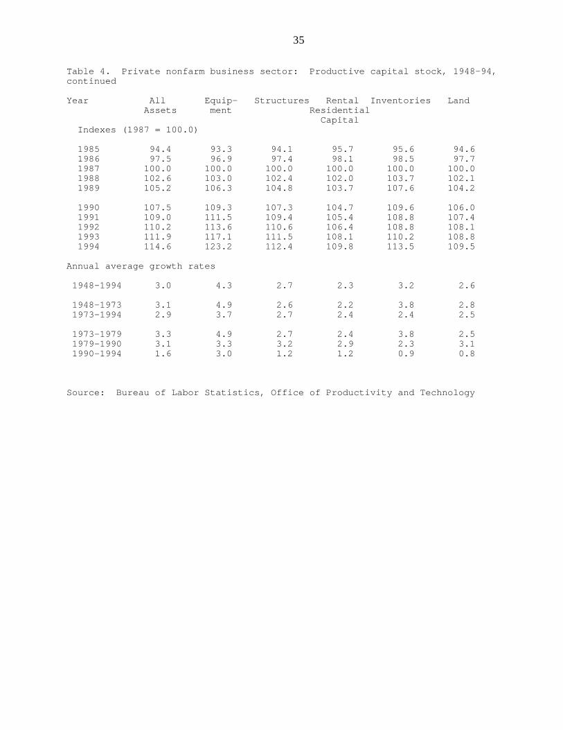
decay functions are important components of this estimation. Table 4 shows the

resulting “productive capital stock” estimates after individual asset types have been

33

aggregated to five broadly-defined categories. All of the data in table 4 are direct

sums of stock over industries and over detailed asset types.

34

Table 4. Private nonfarm business sector: Productive capital stock, 1948-94

Year All Equip- Structures Rental Inventories Land Assets ment Residential Capital Indexes (1987 = 100.0)

1948 29.2 17.5 33.7 38.7 26.8 33.0 1949 29.7 18.8 34.1 39.0 25.7 33.4

1950 30.5 19.8 34.4 39.3 28.3 33.8 1951 31.4 21.1 34.8 39.7 31.6 34.3 1952 32.1 22.3 35.4 39.8 32.5 34.8 1953 32.8 23.5 36.0 40.0 33.1 35.4 1954 33.4 24.6 36.8 40.2 32.4 36.0

1955 34.3 25.8 37.6 40.5 34.4 36.8 1956 35.4 27.1 38.6 40.8 36.2 37.7 1957 36.3 28.4 39.8 41.1 36.1 38.7 1958 37.0 29.2 40.7 41.5 35.5 39.6 1959 37.8 29.8 41.6 42.2 36.6 40.5

1960 38.8 30.6 42.6 42.9 38.4 41.5 1961 39.6 31.4 43.6 43.8 38.3 42.6 1962 40.7 32.1 44.7 45.0 40.0 43.8 1963 42.0 33.2 45.8 46.6 41.6 45.2 1964 43.4 34.5 47.1 48.4 43.6 46.7

1965 45.3 36.4 48.7 50.2 46.3 48.6 1966 47.5 38.9 50.7 51.9 49.8 50.6 1967 49.8 41.5 52.6 53.3 53.8 52.5 1968 51.9 44.0 54.6 54.8 56.7 54.4 1969 54.2 46.8 56.6 56.9 59.5 56.5

1970 56.4 49.5 58.6 59.0 61.3 58.7 1971 58.5 51.7 60.6 61.1 63.1 60.8 1972 60.7 54.1 62.5 63.7 65.1 63.0 1973 63.4 57.3 64.5 66.3 68.7 65.3 1974 66.0 61.1 66.6 68.0 72.7 67.3

1975 67.8 64.0 68.3 68.9 73.1 68.7 1976 69.3 66.1 69.8 69.8 74.7 69.9 1977 71.2 68.8 71.3 71.0 78.2 71.1 1978 73.7 72.3 73.1 72.6 82.4 72.8 1979 77.0 76.5 75.5 76.5 85.7 75.6

1980 80.4 80.2 78.4 82.1 85.7 79.4 1981 83.7 83.4 81.7 87.0 86.5 83.3 1982 86.3 85.7 85.1 89.7 86.3 86.5 1983 88.1 87.4 87.8 91.1 85.0 88.8 1984 90.9 89.8 90.6 93.0 91.1 91.3

35

Table 4. Private nonfarm business sector: Productive capital stock, 1948-94,continued

Year All Equip- Structures Rental Inventories Land Assets ment Residential Capital Indexes (1987 = 100.0)

1985 94.4 93.3 94.1 95.7 95.6 94.6 1986 97.5 96.9 97.4 98.1 98.5 97.7 1987 100.0 100.0 100.0 100.0 100.0 100.0 1988 102.6 103.0 102.4 102.0 103.7 102.1 1989 105.2 106.3 104.8 103.7 107.6 104.2

1990 107.5 109.3 107.3 104.7 109.6 106.0 1991 109.0 111.5 109.4 105.4 108.8 107.4 1992 110.2 113.6 110.6 106.4 108.8 108.1 1993 111.9 117.1 111.5 108.1 110.2 108.8 1994 114.6 123.2 112.4 109.8 113.5 109.5

Annual average growth rates

1948-1994 3.0 4.3 2.7 2.3 3.2 2.6

1948-1973 3.1 4.9 2.6 2.2 3.8 2.8 1973-1994 2.9 3.7 2.7 2.4 2.4 2.5

1973-1979 3.3 4.9 2.7 2.4 3.8 2.5 1979-1990 3.1 3.3 3.2 2.9 2.3 3.1 1990-1994 1.6 3.0 1.2 1.2 0.9 0.8

Source: Bureau of Labor Statistics, Office of Productivity and Technology

36

Table 5. Private nonfarm business sector: Real capital input, 1948-94

Year All Equip- Structures Rental Inventories Land Assets ment Residential CapitalIndexes (1987 = 100.0)

1948 20.1 11.6 25.9 35.5 24.6 25.5 1949 20.5 12.6 26.3 35.8 23.8 26.0

1950 21.5 13.6 26.6 36.3 26.1 26.6 1951 22.8 14.5 27.2 36.7 30.1 27.1 1952 23.8 15.9 28.0 37.0 31.2 27.7 1953 24.6 17.1 28.8 37.3 31.8 28.4 1954 25.2 18.0 29.7 37.6 31.0 29.3

1955 26.2 18.9 30.7 38.0 33.1 30.0 1956 27.3 20.0 32.0 38.5 34.9 30.9 1957 28.2 21.0 33.5 38.9 34.9 32.0 1958 28.8 21.6 34.6 39.4 34.4 33.0 1959 29.5 22.0 35.7 40.2 35.3 33.9

1960 30.5 22.7 36.8 41.0 37.1 34.8 1961 31.2 23.3 38.1 41.9 36.9 35.8 1962 32.3 24.0 39.4 43.1 38.9 36.9 1963 33.5 24.9 40.7 44.7 40.6 38.0 1964 34.8 26.0 42.1 46.5 42.4 39.3

1965 36.7 27.6 43.9 48.3 45.3 41.0 1966 39.0 29.8 46.2 50.0 49.3 42.8 1967 41.4 32.0 48.4 51.4 53.7 44.7 1968 43.4 33.9 50.6 53.0 56.5 46.4 1969 45.6 36.1 52.8 55.1 59.3 48.1

1970 47.7 38.3 55.0 57.2 61.2 49.7 1971 49.6 40.2 57.0 59.5 62.7 51.2 1972 51.7 42.4 58.9 62.3 64.4 52.8 1973 54.5 45.4 60.9 65.1 68.3 55.3 1974 57.5 48.9 63.0 67.1 72.5 57.8

1975 59.7 51.7 64.8 68.2 73.2 60.1 1976 61.6 54.1 66.4 69.2 74.7 62.1 1977 63.8 56.9 68.0 70.5 78.1 64.1 1978 66.8 61.3 70.1 72.4 82.2 66.0 1979 70.3 65.5 72.8 76.3 85.7 68.7

1980 74.2 69.6 76.1 81.6 85.6 73.4 1981 78.2 73.6 80.2 86.1 86.7 78.7 1982 81.6 77.0 84.4 88.8 86.5 82.3 1983 84.1 79.9 87.6 90.2 85.4 85.5 1984 87.7 83.7 90.6 92.2 91.6 89.5

37

Table 5. Private nonfarm business sector: Real capital input, 1948-94,continued

Year All Equip- Structures Rental Inventories Land Assets ment Residential CapitalIndexes (1987 = 100.0)

1985 92.0 89.4 94.1 95.0 95.8 93.1 1986 96.7 95.2 97.3 97.7 99.1 96.6 1987 100.0 100.0 100.0 100.0 100.0 100.0 1988 103.2 104.2 102.3 102.4 103.6 101.9 1989 106.2 108.2 104.7 104.5 107.0 103.7

1990 108.8 111.8 107.1 105.9 108.7 105.2 1991 110.6 114.4 109.1 106.8 107.8 105.8 1992 112.4 116.9 110.5 108.0 109.2 107.2 1993 114.7 121.0 111.4 109.7 110.9 108.4 1994 118.0 127.7 112.3 111.5 113.3 109.4

Annual average growth rates

1948-1994 3.9 5.4 3.2 2.5 3.4 3.2

1948-1973 4.1 5.6 3.5 2.5 4.2 3.2 1973-1994 3.7 5.1 3.0 2.6 2.4 3.3

1973-1979 4.3 6.3 3.0 2.7 3.9 3.7 1979-1990 4.0 5.0 3.6 3.0 2.2 3.9 1990-1994 2.0 3.4 1.2 1.3 1.0 1.0

Source: Bureau of Labor Statistics, Office of Productivity and Technology

38

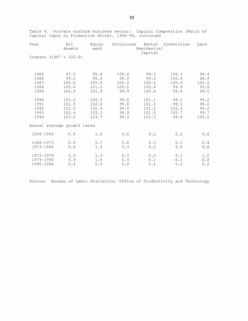
Table 6. Private nonfarm business sector: Capital Composition (Ratio ofCapital Input to Productive Stock), 1948-94

Year All Equip- Structures Rental Inventories Land Assets ment Residential CapitalIndexes (1987 = 100.0)

1948 68.8 66.1 76.8 91.6 91.9 77.1 1949 69.2 66.9 77.2 91.9 92.6 77.8

1950 70.6 68.7 77.5 92.2 92.3 78.5 1951 72.6 69.0 78.1 92.6 95.4 79.0 1952 74.0 71.1 79.0 93.0 96.0 79.7 1953 75.1 72.7 79.9 93.3 96.3 80.4 1954 75.3 73.0 80.8 93.6 95.6 81.2

1955 76.3 73.5 81.8 94.0 96.0 81.4 1956 77.2 73.9 82.9 94.3 96.6 81.8 1957 77.7 74.0 84.1 94.7 96.5 82.5 1958 77.9 73.9 85.1 95.0 96.8 83.2 1959 78.2 73.8 85.8 95.3 96.5 83.6

1960 78.7 74.0 86.6 95.5 96.6 83.9 1961 78.9 74.3 87.4 95.7 96.3 84.1 1962 79.4 74.6 88.1 95.8 97.1 84.1 1963 79.8 75.1 88.8 96.0 97.5 84.1 1964 80.2 75.5 89.5 96.1 97.3 84.2

1965 80.9 76.0 90.2 96.2 97.8 84.3 1966 82.0 76.6 91.1 96.3 99.0 84.7 1967 83.1 77.0 92.0 96.5 99.8 85.1 1968 83.5 77.0 92.7 96.6 99.6 85.2 1969 84.1 77.2 93.3 96.9 99.6 85.1

1970 84.5 77.3 93.8 97.1 99.8 84.7 1971 84.7 77.6 94.1 97.3 99.4 84.2 1972 85.1 78.3 94.3 97.7 98.9 83.7 1973 86.1 79.1 94.5 98.1 99.5 84.8 1974 87.1 80.0 94.6 98.6 99.6 85.9

1975 88.1 80.8 94.9 98.9 100.1 87.5 1976 88.9 81.8 95.2 99.1 100.0 88.9 1977 89.6 82.8 95.4 99.4 99.9 90.2 1978 90.7 84.7 95.9 99.6 99.7 90.7 1979 91.4 85.6 96.4 99.7 100.0 90.9

1980 92.3 86.7 97.0 99.4 99.9 92.4 1981 93.5 88.2 98.1 99.0 100.2 94.4 1982 94.5 89.8 99.2 99.0 100.2 95.1 1983 95.5 91.4 99.7 99.0 100.5 96.2 1984 96.4 93.2 100.0 99.1 100.5 98.0

39

Table 6. Private nonfarm business sector: Capital Composition (Ratio ofCapital Input to Productive Stock), 1948-94, continued

Year All Equip- Structures Rental Inventories Land Assets ment Residential CapitalIndexes (1987 = 100.0)

1985 97.5 95.8 100.0 99.3 100.3 98.4 1986 99.2 98.2 99.9 99.5 100.6 98.9 1987 100.0 100.0 100.0 100.0 100.0 100.0 1988 100.6 101.2 100.0 100.4 99.9 99.8 1989 100.9 101.9 99.9 100.8 99.4 99.5

1990 101.2 102.3 99.8 101.1 99.1 99.2 1991 101.5 102.6 99.8 101.3 99.1 98.6 1992 102.0 102.9 99.9 101.5 100.3 99.2 1993 102.4 103.3 99.9 101.5 100.7 99.7 1994 103.0 103.7 99.9 101.5 99.8 100.0

Annual average growth rates

1948-1994 0.9 1.0 0.6 0.2 0.2 0.6

1948-1973 0.9 0.7 0.8 0.3 0.3 0.4 1973-1994 0.9 1.3 0.3 0.2 0.0 0.8

1973-1979 1.0 1.3 0.3 0.3 0.1 1.2 1979-1990 0.9 1.6 0.3 0.1 -0.1 0.8 1990-1994 0.4 0.3 0.0 0.1 0.2 0.2

Source: Bureau of Labor Statistics, Office of Productivity and Technology

40

In addition to the computation of detailed “productive capital stocks,”

implicit capital rental prices by detailed asset types and by industry are estimated.

These estimated rental prices are used to develop cost-share weights for each

capital category. A Tornqvist aggregate is then computed: annual changes in

logarithms of the capital stock data are weighted by these cost shares. The

resulting series is an estimate of annual “real capital input,” or the estimated flow

of services from the capital stock. These series are shown, again by broad asset

category, in table 5. A third table on capital, table 6, is derived from the first two:

it is capital composition, or the ratio of capital services input to productive capital

stock in the private nonfarm business sector.

Table 6 shows that capital services input generally has risen more rapidly

than capital stock. Over the years 1948-94, the average annual rate of increase in

the input-to-stock ratio was 0.9 percent. This trend reflects an increased annual

rate of services flow from the “average” capital asset and results from a shift in the

composition of assets toward assets with higher estimated rental prices. This trend

is considerably influenced by a long-term trend toward shorter-lived asset types,

which yield their services over a shorter life span and have higher annual rental

prices. In the last few decades, it is likely that rapidly rising corporate spending on

computers is an important factor in this shift to short-lived asset types.

The flow of capital services rose more rapidly than capital stock not only

for all assets over the whole period 1948-94, but also for each broad category of

assets over this period (table 6). And the input-to-stock ratio also rose over all the

sub-periods shown in the table. Note, however, that this ratio rose less rapidly

after 1990 than in earlier time periods.

These trends in capital input in the BLS data have been observable only

because BLS has adopted an index method that accords with research on

aggregation techniques and on the measurement of capital in the production

41

context. The Tornqvist index method is an important element of implementing this

approach. One of the effects of the adoption of this measurement method is that

measured capital input has risen more rapidly, and MFP somewhat less rapidly,

than if capital stocks alone were taken into account.

Labor input

In 1993, BLS introduced Tornqvist indexes of labor composition change

into its major sector MFP series (BLS, Labor Composition and U.S. Productivity

Growth, 1948-90, 1993), as noted above. This study makes use of wage equations

to estimate the prices of detailed types of labor input; the detailed types result

from a cross-classification of hours worked by level of education, gender, and

estimated years of actual work experience (as distinct from potential work

experience). These estimated prices permit the development of estimates of the

annual flow of services, to the production process, from the total of hours worked

in each sector. The difference between this estimated annual flow and the direct

aggregate of hours worked is the contribution to output, and ultimately to

productivity, of changes in the composition of the work force.

Tables 7 and 8 show the most recent BLS estimates of total labor input,

computed as just described; the direct aggregate of all hours worked; and the

difference between the two, or labor composition change. Tables 7 and 8 show

42

Table 7. Labor input, hours and labor composition in privatebusiness, selected years, 1948-94

Year Labor Hours of LaborInput all Persons Composition

Indexes (1987 = 100.0)

1948 64.1 71.2 90.01950 63.0 69.3 90.81955 66.7 71.8 92.91960 66.7 70.7 94.41965 71.2 74.2 96.01970 74.2 76.7 96.71973 78.7 81.8 96.21975 75.7 78.1 96.91979 87.4 90.6 96.51980 86.8 89.7 96.81981 88.0 90.3 97.51982 86.6 87.9 98.51983 88.5 89.5 98.91984 93.7 94.6 99.01985 95.8 96.5 99.31986 96.8 97.0 99.71987 100.0 100.0 100.01988 104.2 103.3 100.81989 107.2 105.9 101.21990 107.8 105.9 101.81991 106.5 103.5 102.91992 107.5 103.2 104.21993 110.4 105.7 104.41994 114.8 109.4 104.9

Average annual growth rates

1948-1994 1.3 0.9 0.3 1948-1973 0.8 0.6 0.3 1973-1994 1.8 1.4 0.4 1973-1979 1.8 1.7 0.0 1979-1990 1.9 1.4 0.5 1990-1994 1.6 0.8 0.8

Source: Bureau of Labor Statistics, Office of Productivity andTechnology

43

Table 8. Labor input, hours and labor composition in privatenonfarm business, selected years, 1948-94

Year Labor Hours of LaborInput all persons Composition

Indexes (1987 = 100.0)

1948 54.2 59.5 91.01950 53.8 58.8 91.51955 59.7 63.6 93.81960 61.4 64.8 94.71965 67.6 70.0 96.61970 72.0 74.3 96.81973 76.9 79.8 96.41975 73.9 76.2 97.01979 86.2 89.4 96.51980 85.7 88.5 96.81981 87.0 89.2 97.51982 85.6 86.8 98.61983 87.6 88.5 98.91984 93.0 93.9 99.01985 95.5 96.2 99.21986 96.6 96.8 99.81987 100.0 100.0 100.01988 103.2 103.5 100.81989 107.6 106.3 101.21990 108.3 106.4 101.81991 106.8 103.8 102.91992 108.0 103.6 104.21993 111.2 106.4 104.51994 115.6 110.1 105.0

Average annual growth rates

1948-1994 1.7 1.3 0.3 1948-1973 1.4 1.2 0.2 1973-1994 2.0 1.5 0.4 1973-1979 1.9 1.9 0.0 1979-1990 2.1 1.6 0.5 1990-1994 1.6 0.9 0.8

Source: Bureau of Labor Statistics, Office of Productivity andTechnology

44

the data for the private business sector and the private nonfarm business sector,

respectively. Generally, the flow of labor services increased more rapidly than the

direct aggregate of hours. For the whole period, 1948-94, total labor input in the

private nonfarm business sector—the flow of services—rose at an average annual

rate of 1.7 percent, while the direct aggregate rose at an average annual rate of

1.3. The difference, 0.3 percent (after rounding), represents the contribution of

change in labor composition to the flow of labor services. Further, for most of the

peak-to-peak cyclical periods shown in tables 7 and 8, the flow of services also

increased more rapidly than aggregate hours. (The data in these two tables were

developed in the process of preparing the data for BLS, Multifactor Productivity

Trends, 1994, January 17, 1996.)

Several results of this analysis are noteworthy. First, the fact that labor

input rose more rapidly than the direct aggregate of hours results in a decrease in

the growth rate of MFP. The actual increase in MFP was lower than the apparent

increase that would have resulted from disregarding the change in labor

composition. (However, note that the contribution of labor composition change is

smaller, for the whole span of years covered, than the 0.3 figure noted above. The

calculation of this contribution must take into account an estimate of the elasticity

of output with respect to labor input; the best estimate of this elasticity is provided

by labor’s share of input, roughly two-thirds at the macro level.) In a sense,

growth in output that would have been deemed to be a result of productivity

change is, following this labor composition study, deemed to be a result of

increasing labor input.

A second noteworthy result is that for the years 1973-79 the growth rate of

labor composition declined to zero. This decline contributed to the dramatic

slowdown in overall productivity growth after 1973. A third important result is

that the growth rate of labor composition change has increased in the 1990s and,

for the first time, is about as large as the growth in the direct aggregate of hours

45

worked; both grew at 0.8 percent in the private business sector and at about the

same rates in private nonfarm business. A fourth result is presented in the bulletin

that introduced these data, but is not evident in tables 7 or 8. To the best of our

ability to determine the sources of labor composition change, the long-term

increase was due predominantly to rising educational levels. In contrast, the

turning points in labor composition trends between sub-periods were apparently

due mainly to changes in work experience. However, the qualification, “to the

best of our ability” is important: BLS researchers concluded that exact measures of

the separate contributions of each component of labor composition change require

a set of highly unlikely assumptions (BLS, Labor Composition and U.S.

Productivity Growth, 1948-90, 1993, Appendix H; see also Rosenblum et al

1990).

Revised output data

The adoption of current-weighted output indexes has also had an important

influence on measured productivity trends. As noted earlier, during the years 1994

to 1996, current-weighted output indexes were introduced for the three BLS

productivity data sets for the United States that were not using such indexes as of

1994. In February 1996, current-weighted output data were incorporated into the

quarterly major sector labor productivity series. The effects on trends in nonfarm

business productivity of introducing the new series are evident through an

examination of table 9, which relates to the nonfarm business sector. The

discussion of table 9 will focus on columns d, e, and f, because these columns

relate solely to the effect of changing the output measure from constant 1987

dollars to annually-weighted output data. (The other columns include the effects

46

of another change in output data, also carried out in February 1996, a change

from income side to product side information.13)

13 The difference between the income side and the product side data is statistical discrepancy.For further discussion of change from income side to product side data, see Dean, Harper andOtto (1995).

47

Table 9. A comparison of old and new measures of output and productivity,nonfarm business sector, compound average annual rates of change (percent)

Output Productivity(a) (b) (c) (d) (e) (f) (g)

Old New Old Old NewConstant Annual Constant Constant Annual

1987 dollars, weighted 1987 dollars, 1987 dollars, weightedincome product income product product Difference Difference

side * side ** side * side * side ** (e)-(d) (e)-(c)

Trends

60-94 3.1 3.4 1.5 1.5 1.8 0.3 0.3 60-73 4.2 4.7 2.5 2.6 3.0 0.4 0.5 73-79 2.5 3.1 0.6 0.7 1.1 0.4 0.5 79-90 2.4 2.6 0.8 0.8 1.0 0.2 0.2 90-94 2.7 2.0 1.8 1.6 1.1 -0.5 -0.7

Single Years

90-91 -1.0 -1.8 1.5 1.3 0.7 -0.6 -0.8 91-92 2.4 3.0 2.7 2.8 3.2 0.4 0.5 92-93 4.1 2.9 1.3 1.2 0.2 -1.0 -1.1 93-94 5.3 4.0 1.9 1.3 0.5 -0.8 -1.4

Recent Quarters

94:1 5.2 0.9 1.7 0.2 -2.5 -2.7 -4.2 94:2 3.2 6.8 -1.4 -0.5 1.9 2.4 3.3 94:3 4.3 4.2 2.7 3.0 2.6 -0.4 -0.1 94:4 7.7 4.2 4.3 2.7 0.9 -1.8 -3.4

95:1 4.5 0.8 2.5 1.3 -1.1 -2.4 -3.6 95:2 2.4 0.5 4.9 4.3 3.0 -1.3 -1.9 95:3 4.9 4.4 2.0 2.0 1.4 -0.6 -0.6

Cyclical Movements

80:1-80:3 -6.1 -6.6 -1.6 -2.8 -2.3 0.5 -0.780:3-81:3 3.8 3.9 2.0 1.9 2.1 0.2 0.1

81:3-82:4 -2.5 -3.1 0.4 -0.3 -0.3 0.0 -0.682:4-90:3 3.8 4.1 1.0 1.1 1.3 0.2 0.3

90:3-91:1 -2.7 -4.6 1.4 0.2 -0.6 -0.9 -2.091:1-95:3 3.8 3.0 2.2 2.0 1.4 -0.6 -0.8

Sources: Bureau of Economic Analysis and Bureau of Labor Statistics, Office of Productivity andTechnology. Prepared by BLS on February 8, 1996.

* Pre-benchmark (before the BEA comprehensive revisions of January 19, 1996)** Post-benchmark (after the BEA comprehensive revisions of January 19, 1996)

48

For the nonfarm business sector, the switch to annually-weighted output

data resulted in a rise of 0.3 percent in long-term (1960-94) average annual growth

in output and productivity. The average annual growth of output per hour

increased from 1.5 percent to 1.8 percent (columns d, e and f). As would have

been expected, in light of the change from constant 1987 computer prices to

contemporaneous computer prices, the upward revision in the growth rate was

largest for the earliest years of this period. In particular, the upward revision in

labor productivity was 0.4 percent for the years 1960-73. And, as expected, for

the years after 1987 the revision was downward. For the years 1990 to 1994, the

downward revision is a half percentage point.

For students of recent productivity trends, a critical question is whether the

post-1973 productivity slowdown has been reversed. The 1987 constant dollar

data show a slowdown from 2.6 percent in the years 1960 to 1973 (see column d)

to 0.7 percent for 1973-79, a drop of 1.9 percent. This slowdown was followed

by a partial recovery in the growth rate. By the years 1990-94, the growth rate

had recovered to 1.6 percent. In contrast, the revised data for nonfarm business

indicate that there is little evidence of a recovery since 1973. Over various sub-

periods since 1973, the growth rate has been close to one percent. It appears,

then, that there is no evidence from these data for nonfarm business of a recovery

from the post-1973 productivity slowdown.

About every five years BEA undertakes a comprehensive revision of the

national income and product accounts. For many years, an essential aspect of the

comprehensive revision was the change in the base year used to compute constant

dollar data for GDP and its major components. For example, as part of the

comprehensive revision completed in December 1991, BEA began presenting its

constant dollar data for GDP, for all years, in prices of 1987, in place of the

previous constant dollar series, prepared using prices of 1982 (see BEA 1991).

BLS, in its capacity as a user of BEA data for output in its major sector labor

49

productivity series, made a practice of introducing the new constant dollar output

series shortly after BEA completed its comprehensive revision.

It is interesting to ask a “what if” question: what revisions to historical

productivity growth rates would BLS have made early in 1996 if BEA had

continued to use constant dollar data, but would have changed at that time from

GDP computed in constant 1987 dollars to 1992 constant dollars? BEA has kindly

provided BLS with 1992 constant dollar data for the nonfarm business sector.

BLS has computed trends in this series, shown in table 10. Table 10 permits a

comparison of the revised output data that BLS actually used in a news release of

February 1996 (column c of table 10), using BEA’s chained Fisher index data for

nonfarm business, with the revisions that BLS would have made if it had continued

using the constant dollar concept, but had switched from 1987 constant dollar data

to 1992 constant dollar data (column d of table 10). Columns c and d both reflect

BEA’s comprehensive revision of January 1996, including improvements made by

BEA in this comprehensive revision that were unrelated to the change in the

weighting scheme. Columns a and b present 1987 constant dollar and annually-

weighted data as they stood prior to the comprehensive revision. All data in this

table are product-side data.

50

Table 10. A comparison of product side measures of output, nonfarm business sector compound average annual rates of change (percent)

(a) (b) (c) (d) (e) (f)

Constant Annual Annual Constant1987 dollars weighted weighted 1992 dollars,

pre- pre- post- post- Difference Differencebenchmark * benchmark * benchmark ** benchmark ** (b)-(a) (c)-(d)

Trends

60-94 3.1 3.4 3.4 3.1 0.3 0.3 60-73 4.2 4.7 4.7 4.3 0.5 0.4 73-79 2.6 2.9 3.1 2.8 0.3 0.3 79-90 2.4 2.6 2.6 2.3 0.2 0.3 90-94 2.5 2.1 2.0 2.0 -0.4 0.0

Single Years

90-91 -1.1 -1.3 -1.8 -1.9 -0.2 0.1 91-92 2.6 2.3 3.0 2.9 -0.3 0.1 92-93 3.9 3.2 2.9 2.9 -0.7 0.0 93-94 4.6 4.1 4.0 4.2 -0.5 -0.2

Recent Quarters

94:1 3.6 3.5 0.9 1.1 -0.1 -0.2 94:2 4.3 4.5 6.8 6.9 0.2 -0.1 94:3 4.6 4.2 4.2 4.6 -0.4 -0.4 94:4 6.0 4.8 4.2 4.7 -1.2 -0.5

95:1 3.3 2.2 0.8 1.0 -1.1 -0.2 95:2 1.8 0.9 0.5 0.6 -0.9 -0.1 95:3 5.0 3.6 4.4 5.0 -1.4 -0.6

Cyclical Movements

80:1-80:3 -7.2 -6.2 -6.6 -6.8 1.0 0.380:3-81:3 3.7 4.3 3.9 3.1 0.6 0.8

81:3-82:4 -3.1 -3.4 -3.1 -2.5 -0.3 -0.682:4-90:3 3.9 4.1 4.1 3.7 0.2 0.4

90:3-91:1 -3.8 -3.9 -4.6 -5.0 -0.1 0.491:1-95:3 3.6 3.0 3.0 3.2 -0.6 -0.1

Sources: Bureau of Economic Analysis and Bureau of Labor Statistics, Office of Productivity andTechnology. Prepared by BLS on April 16, 1996.

* Before the BEA comprehensive revisions of January 19, 1996** After the BEA comprehensive revisions of January 19, 1996

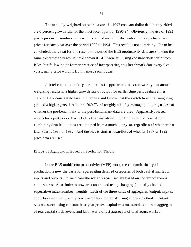
51

The annually-weighted output data and the 1992 constant dollar data both yielded

a 2.0 percent growth rate for the most recent period, 1990-94. Obviously, the use of 1992

prices produced similar results as the chained annual Fisher index method, which uses

prices for each year over the period 1990 to 1994. This result is not surprising. It can be

concluded, then, that for this recent time period the BLS productivity data are showing the

same trend that they would have shown if BLS were still using constant dollar data from

BEA, but following its former practice of incorporating new benchmark data every five

years, using price weights from a more recent year.

A brief comment on long-term trends is appropriate. It is noteworthy that annual

weighting results in a higher growth rate of output for earlier time periods than either

1987 or 1992 constant dollars. Columns e and f show that the switch to annual weighting

yielded a higher growth rate, for 1960-73, of roughly a half percentage point, regardless of

whether the pre-benchmark or the post-benchmark data are used. Apparently, biased

results for a past period like 1960 to 1973 are obtained if the price weights used for

combining detailed outputs are obtained from a much later year, regardless of whether that

later year is 1987 or 1992. And the bias is similar regardless of whether 1987 or 1992

price data are used.

Effects of Aggregation Based on Production Theory

In the BLS multifactor productivity (MFP) work, the economic theory of

production is now the basis for aggregating detailed categories of both capital and labor

inputs and outputs. In each case the weights now used are based on contemporaneous

value shares. Also, indexes now are constructed using changing (annually chained

superlative index number) weights. Each of the three kinds of aggregates (output, capital,

and labor) was traditionally constructed by economists using simpler methods. Output

was measured using constant base year prices; capital was measured as a direct aggregate

of real capital stock levels; and labor was a direct aggregate of total hours worked.

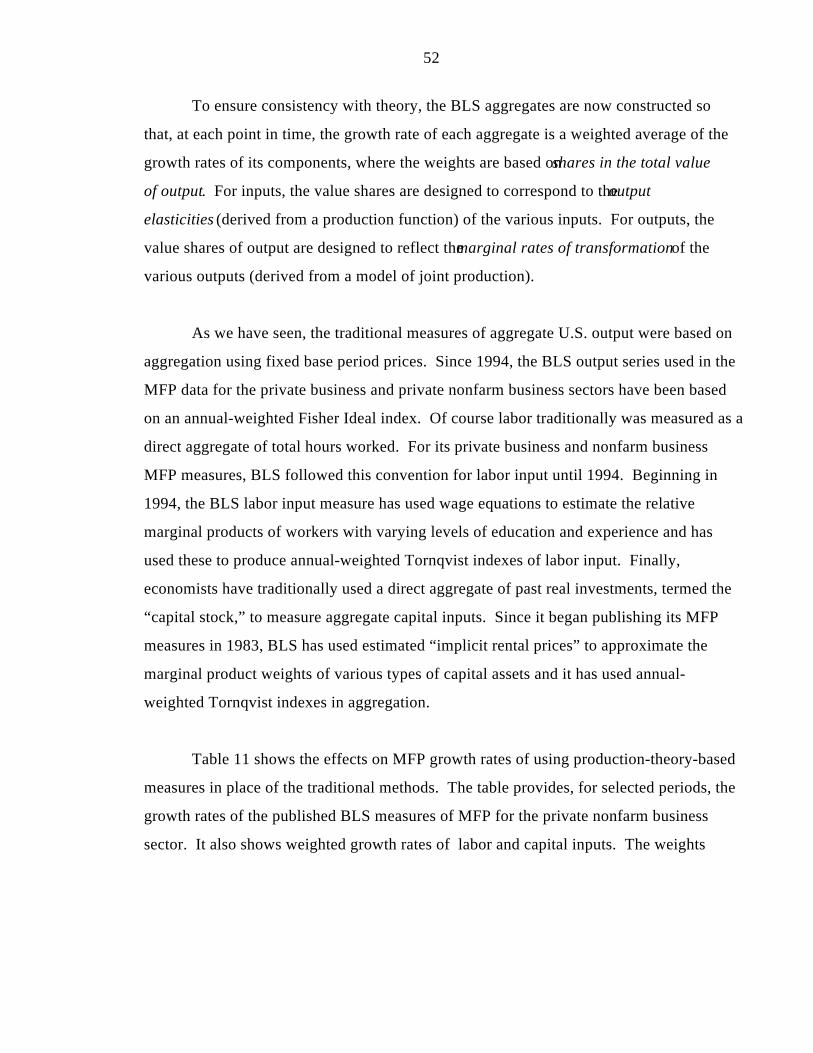
52

To ensure consistency with theory, the BLS aggregates are now constructed so

that, at each point in time, the growth rate of each aggregate is a weighted average of the

growth rates of its components, where the weights are based on shares in the total value

of output. For inputs, the value shares are designed to correspond to the output

elasticities (derived from a production function) of the various inputs. For outputs, the

value shares of output are designed to reflect the marginal rates of transformation of the

various outputs (derived from a model of joint production).

As we have seen, the traditional measures of aggregate U.S. output were based on

aggregation using fixed base period prices. Since 1994, the BLS output series used in the

MFP data for the private business and private nonfarm business sectors have been based

on an annual-weighted Fisher Ideal index. Of course labor traditionally was measured as a

direct aggregate of total hours worked. For its private business and nonfarm business

MFP measures, BLS followed this convention for labor input until 1994. Beginning in

1994, the BLS labor input measure has used wage equations to estimate the relative

marginal products of workers with varying levels of education and experience and has

used these to produce annual-weighted Tornqvist indexes of labor input. Finally,

economists have traditionally used a direct aggregate of past real investments, termed the

“capital stock,” to measure aggregate capital inputs. Since it began publishing its MFP

measures in 1983, BLS has used estimated “implicit rental prices” to approximate the

marginal product weights of various types of capital assets and it has used annual-

weighted Tornqvist indexes in aggregation.

Table 11 shows the effects on MFP growth rates of using production-theory-based

measures in place of the traditional methods. The table provides, for selected periods, the

growth rates of the published BLS measures of MFP for the private nonfarm business

sector. It also shows weighted growth rates of labor and capital inputs. The weights

53

Table 11. Output and Inputs: Measures Based on Production TheoryCompared to Traditional Measures

Estimation of Multifactor Productivity Growth in thePrivate Nonfarm Business Sector

1948- 1973- 1979- 1990- 73 79 90 94

Output Production Theory 4.1 2.9 2.6 2.1 Traditional (Constant 87$) 3.8 2.4 2.7 2.9

Difference 0.3 0.5 -0.1 -0.8

less Weighted Labor Input1

Production Theory 1.0 1.4 1.5 1.2 Traditional 0.8 1.4 1.1 0.6

Difference 0.2 0.0 0.4 0.6

Effects of Education 0.2 0.3 0.3 0.4 Effects of Experience -0.1 -0.3 0.1 0.2 Other Effects 0.0 0.0 0.0 0.0

less Weighted Capital Input1

Production Theory 1.2 1.2 1.2 0.6 Traditional 0.9 0.9 0.9 0.5

Difference 0.3 0.3 0.3 0.1

Multifactor Productivity Production Theory 1.9 0.3 0.0 0.3 Traditional2 2.1 0.1 0.8 1.8

Difference -0.2 0.2 -0.8 -1.5

1 For each pair of successive years, the growth rate of each input ismultiplied by that input’s average share in the value of output for thetwo years. The data reported are averages of this result over the timeperiod.2 The multifactor productivity trend based on production theory minusthe “difference” associated with output plus the sum of the two“differences” associated with labor and capital.

Notes: The “private nonfarm business” sector excludes governmententerprises, while these enterprises are included in the “nonfarmbusiness” sector. Note also that the sums presented in this table maynot equal the totals due to rounding.

54

applied to labor and capital growth rates are the shares of the input in the nominal

value of output. The MFP growth rates at the bottom of the table can be

computed by subtracting the weighted capital and labor input growth rates from

the growth rate of output at the top of the table. The aggregates computed on the

basis of the economic theory of production are labeled “production theory” and are

shown in bold print, while the aggregates based on traditional methods are labeled

“traditional” and are shown in regular type.

For output and both inputs, Table 11 shows the difference between

aggregates based on production theory and traditional aggregates. It is clear that

the measures based on production theory exhibit different magnitudes and time

patterns than the traditional measures. In the case of labor input, the “difference”

corresponds to what BLS calls the “effects of changes in labor composition on

output”. The table further disaggregates this labor composition effect into

separate effects of education, experience and “other” influences (which are

negligible in our measures).

The multifactor productivity growth rate presented in the next-to-last line

of the table, and labeled “production theory,” is the published BLS growth rate of

MFP; this series clearly shows the post-1973 productivity slowdown. The last line

of the table presents ”traditional” MFP growth rates based on traditional output

and input data. The traditional measure can be computed as the multifactor

productivity trend based on production theory minus the “difference” associated

with output plus the sum of the two “differences” associated with labor and

capital. Of course, the “traditional” MFP itself (which involves combining capital

and labor inputs into an index of total input) was derived from production theory.

Nonetheless, Table 11 reflects the measures that would be obtained if production

theory were not applied to the problem of aggregating detailed outputs and inputs.

The data indicate that BLS would obtain a very different pattern of historical MFP

55

growth rates using traditional output and input measures, particularly in the

periods since 1979.

At the beginning of this section of the paper, we stated that it was

important to know whether the improved index number methods described earlier

make a difference in the broad productivity trends shown by the data. The data in

table 11 show that these improved methods make a considerable difference. The

patterns of historical MFP growth rates and the magnitude and timing of the

contributions of capital and labor inputs to output growth differ substantially under

the traditional and the production theory approaches to measurement.

56

6. CONCLUSION

Among the conclusions reached in this paper, the following deserve the

most emphasis.

1. Changing-weight indexes of output and inputs are superior for purposes

of productivity measurement. Among the changing-weight indexes, research by

index number theorists shows that some have superior qualities, and these are most

deserving of consideration by those interested in productivity measurement. The

Tornqvist and Fisher indexes are among those with superior qualities.

2. Application of simple logic and micro-economic theory to the choice of

index number methods also supports the use of changing-weight indexes for

productivity measurement.

3. While the Tornqvist and Fisher indexes both have superior qualities, at

present the Tornqvist index is probably more frequently used for measurement of

multifactor (often referred to as total factor) productivity. Several studies indicate

that trends in Fisher and Tornqvist indexes tend to be quiet similar, but this is not

necessarily the case.

4. Chaining of changing-weight indexes for two periods to form longer-

term time series is common. While direct comparisons between two non-adjacent

points of time are preferable to chaining, some examples indicate that chaining and

direct comparisons sometimes yield similar results.

5. For measurement of industry multifactor productivity, the relevant

literature shows that the sectoral output concept (or the closely-related gross

output concept) is preferable to value added. Some of the arguments for use of

sectoral output in the MFP context carry over to the labor productivity context.

57

6. The adoption of changing-weight indexes can produce substantial

effects on trends in inputs, output, and productivity. An examination of the U.S.

Bureau of Labor Statistics’ changing-weight indexes for the U.S. private nonfarm

business sector demonstrates that they yield substantially different trends than

fixed-weight indexes. Adoption of changing-weight indexes has affected trends for

capital inputs, labor inputs and output in this sector. Adoption of changing-weight

output indexes for the quarterly labor productivity series for nonfarm business has

also led to substantial changes. The effects have been large enough to influence our

understanding of the sources of economic growth.

The organizers of this conference have rightly called attention to the effects

of new measurement procedures on the international comparability of productivity

data. The main implications of this paper for this important subject are the

following.

1. The adoption of changing-weight indexes of output and inputs by the

U.S. Bureau of Labor Statistics is, for the present, yielding one unfortunate result.

The U.S. productivity data are probably less comparable now than they formerly

were to data for countries that use fixed-weight indexes.14

2. Lack of comparability between national productivity measures can arise

from many sources. The Wyckoff (1995) study of national differences in computer

price methodologies provides an example of another source of incomparability,

especially at the level of detailed industries.15 Differences in the industrial

composition of output and in consumption patterns also complicate international

comparisons of productivity. Adoption of similar index number methodologies, by

14 However, see the comment below about the comparability of data in the BLS comparisons ofmanufacturing productivity.15 Note, however, that Wyckoff shows that the differences in national computer pricemethodologies originate in part from use of different index number methods.

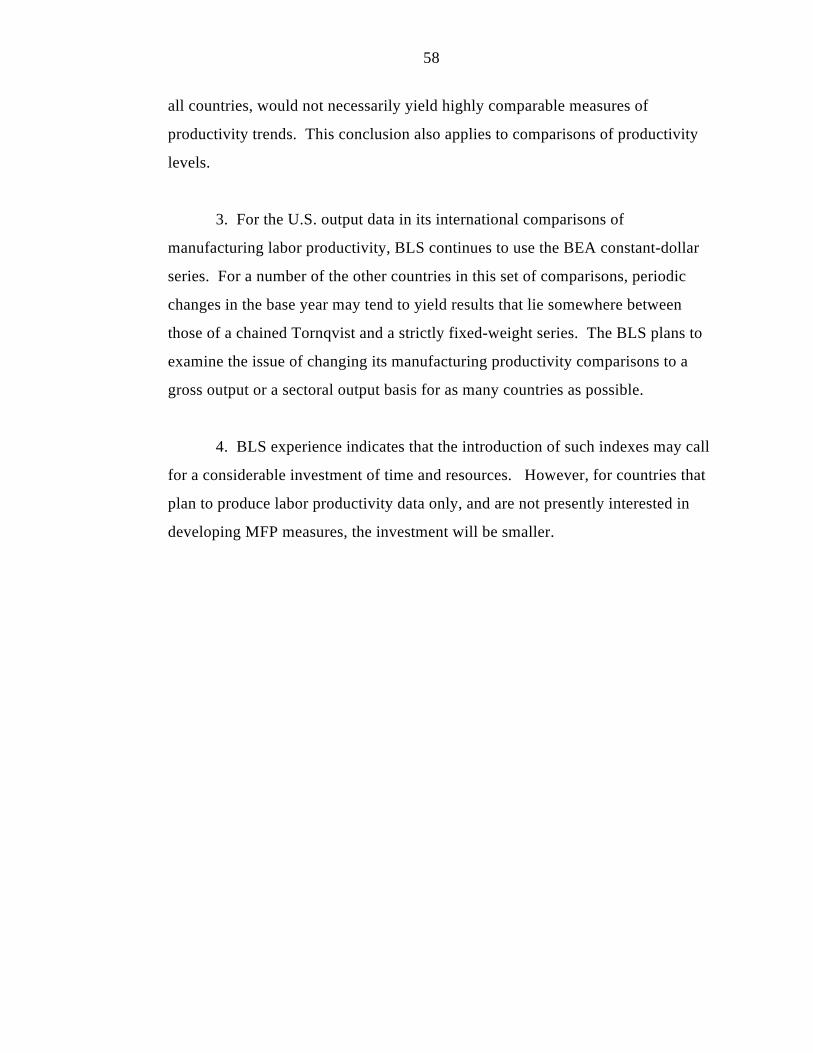
58

all countries, would not necessarily yield highly comparable measures of

productivity trends. This conclusion also applies to comparisons of productivity

levels.

3. For the U.S. output data in its international comparisons of

manufacturing labor productivity, BLS continues to use the BEA constant-dollar

series. For a number of the other countries in this set of comparisons, periodic

changes in the base year may tend to yield results that lie somewhere between

those of a chained Tornqvist and a strictly fixed-weight series. The BLS plans to

examine the issue of changing its manufacturing productivity comparisons to a

gross output or a sectoral output basis for as many countries as possible.

4. BLS experience indicates that the introduction of such indexes may call

for a considerable investment of time and resources. However, for countries that

plan to produce labor productivity data only, and are not presently interested in

developing MFP measures, the investment will be smaller.

59

REFERENCES

Berndt, Ernst, and David O. Wood. 1975. “Technology, Prices, and the DerivedDemand for Energy.” The Review of Economics and Statistics, LVII, No. 3,August: 259-68.

Berndt, Ernst R. and Laurits R. Christensen. 1973. “The Internal Structure ofFunctional Relationships.” Review of Economic Studies, July.

Caves, Douglas W., Laurits R. Christensen, and W. Erwin Diewert. 1982. “TheEconomic Theory of Index Numbers and the Measurement of Input, Output, andProductivity.” Econometrica 50, No. 6, November: 1393-1414.

Christensen, Laurits R., Dale W. Jorgenson, and Lawrence J. Lau. 1973.“Transcendental Logarithmic Production Frontiers.” Review of Economics andStatistics 55, No. 1, February: 28-45.

Dean, Edwin, Kent Kunze, and Larry S. Rosenblum. 1988. “Productivity Changeand the Measurement of Heterogeneous Labor Inputs.” Conference on NewMeasurement Procedures for U.S. Agricultural Productivity. March. (RevisedMarch 1989.)

Dean, Edwin, Michael Harper, and Phyllis Flohr Otto. 1995. “Improvements tothe Quarterly Productivity Measures.” Monthly Labor Review 118, No. 10,October: 27-32.

Denny, Michael and Melvyn Fuss. 1983. “A General Approach to Intertemporaland Interspatial Productivity Comparisons.” Journal of Econometrics 23, No. 3,December: 315-330.

Diewert, W.E. 1976. “Exact and Superlative Index Numbers.” Journal ofEconometrics 4, 115-145.

Diewert, W.E. 1992. “Fisher Ideal Output, Input, and Productivity IndexesRevisited.” The Journal of Productivity Analysis 3, 211-248.

Domar, Evsey D. 1961. “On the Measurement of Technical Change.” EconomicJournal LXX1, No. 284, December: 709-29.

Gollop, Frank M. 1983. “Modeling Aggregate Productivity Growth.” BostonCollege Working Paper, No. 116, January.

Gollop, Frank M. and Dale W. Jorgenson. 1980. “U.S. Productivity Growth byIndustry, 1947-73.” In New Developments in Productivity Measurement and

60

Analysis, John W. Kendrick and Beatrice N. Vaccara, eds., Chicago, University ofChicago Press. 17-136.

Gullickson, William. 1995. “Measurement of Productivity Growth in U.S.Manufacturing.” Monthly Labor Review 118, No. 7, July: 13-28.

Gullickson, William and Michael Harper. 1987. “Multifactor Productivity in U.S.Manufacturing, 1949-83.” Monthly Labor Review 110, No. 10, October: 18-28.

Hall, Robert E. and Dale W. Jorgenson. 1967. “Tax Policy and InvestmentBehavior.” American Economic Review 57, No. 3, June: 391-414.

Harper, Michael J. 1982. “The Measurement of Productive Capital Stock, CapitalWealth, and Capital Services.” Bureau of Labor Statistics Working Paper No.128, June.

Harper, Michael J., Ernst R. Berndt and David O. Wood. 1989. “Rates of Returnand Capital Aggregation Using Alternative Rental Prices”, in Dale W. Jorgensonand Ralph Landau (eds.), Technology and Capital Formation (Cambridge, MA,MIT Press): 331-372.

Hulten, Charles R. 1973. “Divisia Index Numbers” Econometrica 41, No. 6,November: 1017-1025.

Hulten, Charles R., James W. Robertson, and Frank C. Wykoff. 1986. “TheEffects of Energy Price Increases on the Capital Stock in the 1970’s.” January.

Jorgenson, Dale W. and Barbara M. Fraumeni. 1989. “The Accumulation ofHuman and Nonhuman Capital, 1948-1984.” In The Measurement of Saving,Investment, and Wealth, Robert E. Lipsey and Helen S. Tice (eds.), Chicago,University of Chicago Press. 227-282.

Jorgenson, Dale W., Frank M. Gollop, and Barbara M. Fraumeni. 1987.Productivity and U.S. Economic Growth. Cambridge, MA, Harvard UniversityPress. 211-60.

Jorgenson, Dale W. and Zvi Griliches. 1967. “The Explanation of ProductivityChange.” Review of Economic Studies XXXIV(3), No. 99, July: 249-283.

Kunze, Kent, Mary Jablonski, and Virginia Klarquist. 1995. “BLS ModernizesIndustry Labor Productivity Program.” Monthly Labor Review 118, No. 7, July:3-12.

Lysko, Wolodar. 1995. “Manufacturing Multifactor Productivity in ThreeCountries.” Monthly Labor Review 118, No. 7, July: 39-55.

61

Morrison, Catherine J. 1993. “A Microeconomic Approach to the Measurementof Economic Performance.” New York, Springer-Verlag.

Powers, Susan G. 1988. “The Role of Capital Discards in MultifactorProductivity Measurement.” Monthly Labor Review. June: 27-35.

Rosenblum, Larry, Edwin Dean, Mary Jablonski, and Kent Kunze. 1990.“Measuring Components of Labor Composition Change.” Presented at annualmeeting of American Economic Association. December.

Sherwood, Mark K. 1987. “Performance of Multifactor Productivity in the Steeland Motor Vehicle Industries.” Monthly Labor Review, August: 22-31.

Solow, Robert M. 1957. “Technical Change and the Aggregate ProductionFunction.” Review of Economics and Statistics39, No. 3, August: 312-20.

Tornqvist, Leo. 1936. “The Bank of Finland’s Consumption Price Index.” Bankof Finland Monthly Bulletin, No. 10, 1-8.

Triplett, Jack E. 1988. “Superlative and Quasi-Superlative Indexes of Price andOutput for Investment Goods: Office, Computer, and Accounting Machinery.”BEA Discussion Paper No. 40, Presented at a National Bureau of EconomicResearch Summer Workshop, Boston MA, July.

U.S. Bureau of Economic Analysis. 1991. “The Comprehensive Revision of theU.S. National Income and Product Accounts: A Review of Revisions and MajorStatistical Changes.” Survey of Current Business 71, No. 12, December: 24-42.

U.S. Bureau of Economic Analysis. 1995. “Preview of the ComprehensiveRevision of the National Income and Product Accounts: BEA’s New FeaturedMeasures of Output and Prices,” Survey of Current Business 75, No. 7. July: 31-43.

U.S. Bureau of Economic Analysis. 1996. “Improved Estimates of the NationalIncome and Product Accounts for 1959-95: Results of the ComprehensiveRevision,” Survey of Current Business 76, No. 1-2. January-February: 1-31.

U.S. Bureau of Labor Statistics. 1983. Trends in Multifactor Productivity, 1948-81. Bulletin 2178.

U.S. Bureau of Labor Statistics. 1993. Labor Composition and U.S. ProductivityGrowth, 1948-90. Bulletin 2426.

62

U.S. Bureau of Labor Statistics. 1994. “Multifactor Productivity Measures, 1991and 1992.” News Release No. 94-327. July 11.

U.S. Bureau of Labor Statistics. 1995. “International Comparisons ofManufacturing Productivity and Unit Labor Cost Trends, 1994,” News ReleaseNo. 95-342, September 8.

U.S. Bureau of Labor Statistics. 1995. Productivity Measures for SelectedIndustries and Government Services. Bulletin 2461.

U.S. Bureau of Labor Statistics. 1996. “Multifactor Productivity Trends, 1994.”News Release No. 95-518, January 17.

U.S. Bureau of Labor Statistics. 1996. “Productivity and Costs, Third Quarter1995.” News Release No. 96-37, February 8.

Wyckoff, Andrew W. 1995. “The Impact of Computer Prices on InternationalComparisons of Labour Productivity.” Econ. Innov. New Techn. 3: 277-293.

Young, Allan H. 1989. “Alternative Measures of Real GNP.” Survey CurrentBusiness 69, April: 27-34.

Young, Allan H. 1992. “Alternative Measures of Change in Real Output andPrices.” Survey of Current Business 72, April: 32-48.