NBER WORKING PAPER SERIES

PRODUCT DIFFERENTIATION, MULTI-PRODUCT FIRMS AND ESTIMATINGTHE IMPACT OF TRADE LIBERALIZATION ON PRODUCTIVITY

Jan De Loecker

Working Paper 13155http://www.nber.org/papers/w13155

NATIONAL BUREAU OF ECONOMIC RESEARCH1050 Massachusetts Avenue

Cambridge, MA 02138June 2007

An earlier version of this paper was circulated under the title "Product Differentiation, Multi-ProductFirms and Structural Estimation of Productivity". I am especially grateful to Joep Konings, Marc Melitzand Ariel Pakes for comments and suggestions. I would also like to thank Dan Ackerberg, Steve Berry,David Blackburn, Mariana Colacelli, Bronwyn Hall, Amil Petrin, Frank Verboven, Patrick Van Cayseeleand Hylke Vandenbussche for discussions on earlier versions. This paper has benefited from seminarparticipants at University of Minnesota, Yale, Louvain-la-Neuve, KU Leuven, Princeton, NYU, Uof Toronto, UT Austin, UCSC, IESE, Federal Board of Governors, LSE, WZB, NY Fed and conferenceparticipants at IIOC 2005, CEPR Applied IO Workshop 2005, NBER Summer Institute ProductivityWorkshop 2005, Midwest Meeting in International Economics 2005, NBER Productivity Workshop2006, EIIT 2007. Furthermore, I would like to thank Roberta Adinolfi of EURATEX, Sylvie Groeninckof FEBELTEX, Yannick Hamon and Ignacio Iruarruzaga Diez at the European Commission for providingme with the relevant conversion tables to construct the quota data set. Contact Author: jdl16@nyu.edu.The views expressed herein are those of the author(s) and do not necessarily reflect the views of theNational Bureau of Economic Research.

© 2007 by Jan De Loecker. All rights reserved. Short sections of text, not to exceed two paragraphs,may be quoted without explicit permission provided that full credit, including © notice, is given tothe source.

Product Differentiation, Multi-product Firms and Estimating the Impact of Trade Liberalizationon ProductivityJan De LoeckerNBER Working Paper No. 13155June 2007, Revised November 2007 JEL No. F13,L11

ABSTRACT

In this paper I analyze the productivity gains from trade liberalization in the Belgian textile industry.So far, empirical research has established a strong relationship between opening up to trade and productivity,relying almost entirely on deflated sales to proxy for output in the production function. The latter impliesthat the resulting productivity estimates still capture price and demand shocks which are most likelyto be correlated with the change in the operating environment, which invalidate the evaluation of thewelfare implications. In order to get at the true productivity gains I propose a simple methodologyto estimate a production function controlling for unobserved prices by introducing an explicit demandsystem. I combine a unique data set containing matched plant-level and product-level informationwith detailed product-level quota protection information to recover estimates for productivity as wellas parameters of the demand side (markups). I find that when correcting for unobserved prices anddemand shocks, the estimated productivity gains from relaxing protection are only half (from 8 toonly 4 percent) of those obtained with standard techniques.

Jan De LoeckerStern School of BusinessNew York University44 West Fourth StreetNew York, NY 10012and NBERjdl16@nyu.edu

1 Introduction

Over the last years a large body of empirical work has emerged that relies on the estimation

of production functions to evaluate the impact of policy changes on the efficiency of producers

and the industry as a whole. The reason for this is at least twofold. First of all, there is a

great interest in evaluating active policy changes such as trade liberalization, deregulation and

privatization of industries. One of the questions that typically arise is whether the policy change

had any impact on the efficiency of firms in the economy. It is in this context that the ability

to estimate a production function using micro data (firm-level) is important as it allows us

to recover a measure for (firm-level) productivity and relate this to changes in the operating

environment. Secondly, the increased availability of firm-level datasets for various countries and

industries has further boosted empirical work analyzing productivity dynamics. Out of these set

of papers, a robust result is that periods of changes in the competitive environment of firms -

like trade liberalization - are associated with measured productivity gains and that firms engaged

in international trade (through export or FDI) have higher measured productivity.1

The productivity measures that are used to come to these conclusions are, however, recovered

after estimating (some form of) a sales generating production function where output is replaced

by sales. The standard approach has been to use the price index - of a given industry - to

proxy for these unobserved prices. The use of the price index is only valid if all firms in the

industry face the same output price and corresponds with the assumption that firms produce

homogeneous products and face a common and infinite price elasticity of demand (Melitz, 2001).

In the case of differentiated products this implies that the estimates of the input coefficients are

biased and in addition lead to productivity estimates that capture markups and demand shocks.2

In a second step these productivity estimates are then regressed on variables of interest, say the

level of trade protection or tariffs. This implies that the impact on actual productivity cannot be

identified - using a two-step procedure - which invalidates evaluation of the welfare implications.

In this paper I analyze the productivity gains from trade liberalization in the Belgian textile

industry. As in most empirical work that has addressed similar questions, I do not observe out-

put at the firm level and therefore unobserved prices and demand shocks need to be controlled

for. In order to answer this question, I first introduce a simple methodology for getting reliable

estimates of productivity in an environment of imperfect competition in the product market

where I allow for multi-product firms. The estimation strategy is related to the original work

of Klette and Griliches (1996) where the bias of production function coefficients due to using

deflated firm-level sales (based on an industry-wide producer price index) to proxy for firm-level

1Pavcnik (2002) documents the productivity gains from trade liberalization in Chile, Smarzynska (2004) findspositive spillovers from FDI in Lithuania and Van Biesebroeck (2005) finds learning by exporting in Sub-SaharanAfrican manufacturing. Olley and Pakes (1996) analyze the productivity gains from deregulating the US telecomequipment industry.

2Obtaining precise productivity estimates by filtering out price and demand shocks has a wide range of im-plications for other applied fields. For instance in applying recently developed methods to estimate dynamic(oligopoly) games where productivity is a key primitive (Collard-Wexler 2006).

2

output is discussed. In their application the interest lies in recovering reliable estimates for

returns to scale and not in productivity estimates per se. At the same time a literature emerged

trying to correct for the simultaneity bias without relying on instruments in order to recover

reliable estimates for productivity. The latter is a well documented problem when estimating a

production function with OLS that inputs are likely to be correlated with unobserved produc-

tivity shocks and therefore lead to biased estimates of the production function. Olley and Pakes

(1996) introduced an empirical strategy based on a theoretical dynamic optimization problem of

the firm under uncertainty where essentially unobserved productivity in the production function

is replaced with a polynomial in investment and capital. A series of papers used this approach

to verify the productivity gains from changes in the operating environment of firms such as

trade liberalization, trade protection among others. In almost all of the empirical applications

the omitted price variable bias was ignored or assumed away.3 In this paper I analyze produc-

tivity dynamics during a period of trade liberalization while correcting both for the omitted

price variable and the simultaneity bias. I use the Olley and Pakes (1996) procedure to control

for the simultaneity bias and their framework turns out to be very instructive to evaluate the

importance of demand shocks in the production function and how they affect the productivity

estimates.4 In addition, to correct for the omitted price variable bias and obtain unbiased co-

efficients of the production function, I introduce a rich source of product-level data matched to

the production dataset. This unique additional piece of information allows me to introduce a

richer demand system and recover markup estimates in addition to estimates for productivity

which are the ultimate goal. I empirically show that the traditional ‘productivity measures’

still capture price and demand shocks which are likely to be correlated with the change in the

operating environment.

I find that in my data the omitted price variable bias works in the opposite way and matters

more than the simultaneity and the selection bias. An important implication is that my estimates

for returns to scale are significantly higher than one.5 Furthermore, my results suggest that

only half of the measured productivity gains established using standard techniques capture true

productivity gains. The estimated productivity gains from relaxing quota protection are (on

average) 4 percent in contrast to 8 percent when we ignore the fact that firm-level revenue

captures variation in prices as well.

My framework suggests that the channel through which trade liberalization impacts pro-

ductivity is mostly by cutting off the inefficient producers from the productivity distribution

and therefore increases the average productivity of the industry. However, the (within-firm)

3Some authors did explicitly reinterpret the productivity measures as sales per input measures. For instancesee footnote 3 on page 1264 of Olley and Pakes (1996).

4This does not rule out the use of alternative proxy estimators such as the estimator suggested by Levinsohnand Petrin (2003), however, with some additional assumptions made on the relation between the unobservedproductivity shocks and markups. See Appendix C for a discussion on this.

5 It is actually quite surprising that in recent papers relying on various proxy estimators to control for thesimultaneity bias, almost no increasing returns to scale are established for those industries with high fixed costswhere we would expect to find them.

3

productivity gains for those producers that remain active are small and sometimes even negligi-

ble. These two observations then imply a very different interpretation of how opening up trade

impacts individual firms. Furthermore, the reallocation of activities across surviving firms is not

as closely tied to productivity, but rather an interplay of the ability to markup over costs and

productivity.

Combing a production function and a demand system into one framework provides other

interesting results and insights with respect to the product mix and market power. I find that

including the product mix of a firm is an important dimension to consider when analyzing

productivity dynamics. Even if this has no impact on the aggregation of production across

products, it matters since it allows to estimate different markups across product segments. In

the context of the estimation of production functions multi-product firms have not received a lot

of attention with the exception of the theoretical work of Melitz (2001). The main reason for this

is the lack of detailed product-level production data: inputs (labor, material and capital) usage

and output by product and firm. Ignoring the product-level dimension has some important

implications on the production technology we assume, i.e. no cost synergies or economies of

scope are allowed. In my data I only observe the number of products produced per firm and

where these products are located in product space (segments of the industry). This does not

allow me to depart from the standard modeling assumptions on the production side as in Melitz

(2001). But it does allow me to specify a richer demand system and therefore enables me to

investigate the productivity response controlling for price and markup effects. For the latter

it is crucial to introduce products as the quota protection that are used at the EU level vary

greatly across product categories. This however does not capture the channel recently described

by Bernard et. al (2003). They document the importance of product mix variation across

producers in a given industry and how firms respond to shocks (trade liberalization) along this

dimension.6

A growing number of papers have studied the impact of various trade policy changes on

productivity in the absence of market power.7 By introducing a rich source of demand variation

I am able to decompose the traditional measured productivity gains into real productivity gains

and demand side related components and evaluate whether opening up to trade is truly changing

the efficiency of producers. In addition, the method sheds light on other parameters of interest

such as markups. I estimate markups ranging from 0.16 for the interior segment to 0.23 in the

clothing segment of the textile industry. These numbers are in line with what other studies have

found relying on different methods. In the context of trade liberalization, a number of authors

have found strong relationships between trade protection and markups (Konings and Vanden-

bussche, 2005). My results therefore shed light on the importance of both the productivity and

markup response to a change in a trade regime.

6These authors define a product as a 5 digit industry code which is a product line. I refer to a product as an 8digit product code which implies that we expect to see - if anything - bigger numbers on for instance the numberof products per firm.

7See Tybout (2000) for a review on the relationship between openness and productivity in developing countries.

4

Recent work has discussed the potential bias of ignoring demand shocks when estimating

production functions based on deflated firm-level sales to proxy for output. Katayama et al.

(2003) start out from a nested logit demand structure and verify the impact of integrating a

demand side on the interpretation of productivity. Melitz and Levinsohn (2002) assume a rep-

resentative consumer with Dixit-Stiglitz preferences and they feed this through the Levinsohn

and Petrin (2003) estimation algorithm.8 Foster, Haltiwanger and Syverson (forthcoming) dis-

cuss the relation between physical output, revenue and firm-level prices. They study this in

the context of market selection and they state that productivity based upon physical quantities

is negatively correlated with establishment-level prices while productivity based upon deflated

revenue is positively correlated with establishment-level prices. The few papers that explicitly

analyze the demand side when estimating productivity or that come up with a strategy to do so

all point in the same direction: estimated productivity still captures demand related shocks.9

The remainder of this paper is organized as follows. In section 2 the standard approach to

estimate production functions is discussed and I introduce a demand system and show the bias

on the production function coefficients. Section 3 introduces the estimation strategy and the

potential bias of using standard productivity estimates to evaluate policy changes. In section 4,

I present the data that includes detailed product-level information in addition to a rich firm-level

dataset of Belgian textile producers. In section 5 I present the coefficients of the production

functions as well as the estimated parameters of the demand system. In section 6 I analyze the

effects of the trade liberalization episode in the EU textiles on productivity, where the trade

liberalization is measured by the drastic fall in product specific quota protection. The quota

information also serves as an important control variable for the unobserved prices through the

introduction of the demand system. The last section concludes.

2 Estimating productivity using production data

I briefly review the traditional problems one runs into when estimating a production function

using typical production data on revenue and various inputs of a sample of firms. Given the

focus is on controlling for unobserved firm specific prices and demand shocks, I will discuss the

advantages of specifying an explicit demand system in more detail. Finally, I show how having

information on the product mix of firms allows me to estimate a less restrictive substitution

pattern across the products of the industry.

2.1 Identification of the production function parameters

Let us start with the production side where a firm i at time t produces (a product) according

to the following production function

8 I will come back to the exact differences and extensions of my methodology compared to Melitz (2001) andLevinsohn and Melitz (2002) theoretical setup.

9See Bartelsman and Doms (2000) for a comprehensive review on recent productivity studies using micro data.Concerning the topic of this paper I refer to page 592.

5

Qit = Lαlit M

αmit Kαk

it exp(α0 + ωit + uqit) (1)

where Qit stands for the quantity produced, Lit, Mit and Kit are the three inputs labor, mate-

rials and capital; and αl, αm and αk are the coefficients, respectively.10 The constant term α0

captures the mean productivity and γ captures the economies of scale, i.e. γ = (αl+αm +αk).

Productivity is denoted by ωit and uqit is an i.i.d. component.

The standard approach in identifying the production function coefficients starts out with a

production function as described in equation (1). The physical output Qit is then substituted

by deflated revenue (fRit) using an industry price deflator (PIt). Taking logs of equation (1) and

relating it to the (log of) observed revenue per firm rit = qit+pit, we get the following regression

equation

rit = xitα+ ωit + uqit + pit (2)

where xitα = α0 + αllit + αmmit + αkkit. The next step is to use the industry wide price index

pIt and subtract it from both sides to take care of the unobserved firm-level price pit.

erit = rit − pIt = xitα+ ωit + (pit − pIt) + uqit (3)

Most of the literature on the estimation of productivity has worried about the correlation be-

tween the chosen inputs xit and the unobserved productivity shock ωit. The coefficient on the

freely chosen variables labor and material inputs will be biased upwards as a positive produc-

tivity shock leads to higher labor and material usage (E(xitωit) > 0).

Even if this is corrected for, from equation (3) it is clear that if firms produce differentiated

products or have some pricing power the estimates of α will be biased. As mentioned in Klette

and Griliches (1996) inputs are likely to be correlated with the price a firm charges.11 The error

term (uqit+pit−pIt) still captures firm-level price deviation from the average (price index) priceused to deflate the firm-level revenues. Essentially, any price variation (at the firm level) that is

correlated with the inputs biases the coefficients of interest (α) as E(xit(pit−pIt)) 6= 0. The signof the bias could go either way as it depends on the correlation between the price a firm charges

and the level of its inputs which works through the output of a firm. Therefore firm-level inputs

(materials and labor) are correlated with the unobserved price and thus under- or overestimates

the coefficients on labor and materials. This is referred to as the omitted price variable bias.

Another source of bias is introduced by unobserved demand shocks that might lead to a higher

price and induces a correlation between inputs and price.

The omitted price bias might work in the opposite direction as the simultaneity bias - the

correlation between the unobserved productivity shock (ωit) and the inputs (xit) - making any

10The Cobb-Douglas production function assumes a substitution elasticity of 1 between the inputs. The re-mainder of the paper does not depend on this specific functional form. One can assume e.g. a translog productionfunction and proceed as suggested below.11The interpretation of the correlation is somewhat different here since my model is estimated in log levels and

not in growth rates as in Klette and Griliches (1996).

6

prior on the total direction of the bias hard. It is also clear that even when the marginal product

of the inputs (α) are not of interest, the productivity estimate is misleading as it still captures

price and consequently demand shocks.

The same kind of reasoning can be followed with respect to the measurement of material

inputs where often a industry wide material price deflator is used to deflate firm-level cost of

materials. However, controlling for unobserved prices takes - at least partly - care of this. The

intuition is that if material prices are firm specific, a higher material price will be passed through

a higher output price if output markets are imperfect, the extent of this pass through depends

on the relevant markup. The only case where this reasoning might break down is when input

markets are imperfect and output markets are perfectly competitive, which is not a very likely

setup.12

2.2 Introducing demand and product differentiation

I now introduce the demand system that firms face in the output market. Firms are assumed to

operate in an industry characterized by horizontal product differentiation, where η captures the

substitution elasticity among the different products in a segment and η is finite. As mentioned

in Klette and Griliches (1996) similar demand systems have been used extensively under the

label of Dixit-Stiglitz demand. The key feature is that monopolistic competition leads to price

elasticities which are constant and independent of the number of varieties.13 In addition, I

explicitly introduce unobserved demand shocks that are allowed to be correlated with price and

other demand conditions. In the empirical application I will use product-firm dummies and

product specific quota restrictions as additional controls.

The introduction of an explicit demand side into the revenue production function is very

closely related to the model of Melitz and Levinsohn (2002) and Klette and Griliches (1996).

However, there are some important differences and extensions I suggest. Firstly, in addition to

the plant-level dataset I will introduce product-level information matched to the plants allowing

me to put more structure on the demand side. They proxy the number of products per firm

by the number of firms in an industry, while I observe the actual number of products produced

by each firm and additional demand related variables. I use this additional source of variation

to identify the elasticity of substitution for different segments of the industry. Secondly, aside

from a discussion of the methodology, I empirically show the bias in the production function

coefficients and in the resulting productivity estimates. Finally, I use segment demand shifts,

product dummies and product specific quota restrictions to further instrument for demand

12 If material prices differ across firms, an additional correlation of the input with the unobserved price pi isintroduced through the correlation between output prices pi and material prices pmi . Note that this is in additionto the correlation between material mi used and prices pi.This follows from the fact that deflated material costscan be written as (mi + pmi − pmI ).13The choice of this conditional demand system does not rule out other specifications to be used in the remainder

of the paper. However, it implies that the inverse of the elasticity of substitution (demand ) is the relevant markupas the substitution elasticity with respect to other goods (non textile products) is zero.

7

shocks to obtain consistent estimates of the supply side parameters as they provide an exogenous

source of demand side shifts. I rely on my estimates to analyze the potential (within-firm)

productivity gains from the trade liberalization episode in the EU textile industry. The structure

of the demand system I build on implies that all unobserved demand shocks shift the individual

firm’s demand intercept around.

It is clear that the demand system is quite restrictive and implies one single elasticity of

substitution for all products within a given product range - segment - and hence no differences

in cross price elasticities. In the empirical application the elasticity of substitution is allowed to

differ among product segments. This is in contrast to the commonly used (implicit) assumption

that all firms face one infinite price elasticity of demand. The motivation for modeling demand

explicitly here is to control for unobserved price variation. However the final interest lies in an

estimate of productivity and further relaxing the substitution patterns here would just reinforce

the argument.

The choice of demand system needed to identify the parameters of interest is somewhat

limited due to missing demand data, i.e. prices and quantities. Therefore, one has to be willing

to put somewhat more structure on the nature of demand. However, the modeling approach

here does not restrict any demand system as long as the inverse demand system can generate a

(log-) linear relationship of prices and quantities.

I start out with single product firms and show how this leads to my augmented production

function. In a second step I allow for firms to produce multiple products. The focus is on the

resulting productivity estimates and in the case of multi-product firms these can be interpreted

as average productivity across a firm’s products.

2.2.1 A Simple Demand Structure: Single Product Firms

I follow Klette and Griliches (1996) and later on I extend it by allowing firms to produce multiple

products. I start out wit a simple (conditional) demand system where each firm i produces a

single product and faces the following demand Qit

Qit = QIt

µPitPIt

¶η

exp(udit + ξit) (4)

where QIt is an aggregate demand shifter and here directly relates to the industry output at

time t. As noted by Klette and Griliches (1996) this industry output can easily be computed

using firm-level revenues and the producer price index of the industry.14 Industry output QIt is

simply a weighted average of the deflated revenues QIt = (PN

i msitRit)/PIt where the weights

(msit) are the market shares. This observation is important for the empirical analysis where

I will use this notion to construct segment-specific output (demand shifters) using firm-specific

product mix information. (Pit/PIt) is the relative price of firm i with respect to the average price

14This comes from the observation that a price index is essentially a weighted average of firm-level prices whereweights are market shares (see Appendix A.2). Under the given demand structure it follows that (the first orderproxy for) the price index is a market share weighted average of the firm-level prices.

8

in the industry, udit is an idiosyncratic shock specific to firm i and η is the substitution elasticity

between the differentiated products in the industry, where −∞ < η < −1. As mentioned

above, I allow for unobserved demand shocks ξit to be correlated with price and the observed

demand shifters. In discrete choice models like Berry (1994) and Berry, Levinsohn and Pakes

(1995) where observed product characteristics are introduced this unobserved demand shock ξitis interpreted as (product) quality.

Taking logs of equation (4) and writing the price as a function of the other variables results

in the following expression where xit = lnXit

pit =1

η(qit − qIt − udit − ξit) + pIt (5)

As discussed extensively in Klette and Griliches (1996) and Melitz and Levinsohn (2002),

the typical firm-level dataset has no information on physical output per firm and prices.15

Commonly, we only observe revenue and we deflate this using an industry-wide deflator. The

observed revenue rit is then substituted for the true output qit when estimating the production

function. I now substitute expression (5) for the price pit in equation (2) to get an expression

for revenue. From here forward, I consider deflated revenue (erit = rit − pIt)

erit = rit − pIt =

µη + 1

η

¶qit −

1

ηqIt −

1

η(udit + ξit) (6)

Now I only have to plug in the production technology as expressed in equation (1) and I have a

revenue generating production function with both demand and supply variables and parameters.

erit = µη + 1η

¶(α0 + αllit + αm mit + αkkit)−

1

ηqIt +

µη + 1

η

¶(ωit + uqit)−

1

η(udit + ξit)

It is clear that if one does not take into account the degree of competition on the output

market (firm price variation), that the analysis will be plagued by an omitted price variable bias

and the estimated coefficients are estimates of a reduced form combining the demand and supply

side in one equation. This leads to my general estimating equation of the revenue production

function erit = β0 + βllit + βm mit + βkkit + βηqIt + (ω∗it + ξ∗it) + uit (7)

where βh = ((η + 1)/η)αh with h = l,m, k; βη = −η−1, ω∗it = ((η + 1)/η)ωit, ξ∗it = −η−1ξit anduit = ((η+1)/η)u

qit− 1

ηudit. When estimating this equation (7) I recover the production function

coefficients (αl, αm , αk) and returns to scale parameter (γ) controlling for the omitted price

variable and the simultaneity bias, as well as an estimate for the elasticity of substitution η. In

fact, to obtain the true production function coefficients (α) I have to multiply the estimated

reduced form parameters (β) by the relevant markup ( ηη+1). When correcting for the simultaneity

15Exceptions are Dunne and Roberts (1992), Jaumandreu and Mairesse (2004), Eslava et al.(2004) and Fosteret al. (2005) where plant-level prices are observed and thus demand and productivity shocks can be estimatedseparately. To my knowledge this is a very rare setup.

9

bias I follow the Olley and Pakes (1996) procedure and replace the productivity shock ωit by a

function in capital and investment.

In my empirical analysis I will estimate various versions of (7) as the product information

linked to every firm allows me to put more structure on the demand side, e.g. allowing the

demand elasticity to vary across different segments and proxy for unobserved demand shocks

(ξit) using product dummies. Adding the extra information from the product space is not

expected to change the estimated reduced form coefficients (β), but it will have an impact on

the estimated demand parameter η and hence on the true production function coefficients (α).16

2.2.2 Multi-product firms

I now allow firms to produce multiple products and the demand system is identical to the one

expressed in equation (4), only a product subscript j is added. Note that the demand is now

relevant at the product level. There are N firms and M products in the industry with each firm

producing Mi products, where M =P

iMi.17 I divide the industry into S segments that each

capture a part of the various products in the industry and I allow for segment specific price

elasticities of demand. In the single product case the demand system is the same for every firm

i, whereas in the multiple product case the demand is with respect to product j of firm i.

Qijt = QIst

µPijtPIst

¶ηs

exp(udijt + ξijt) (8)

The demand for product j of firm i is given by Qijt, QIst is the demand shifter relevant at the

product-level, PIst is the industry price index relevant at the product level, ηs is the demand

elasticity relevant at the segment level, ξijt is unobserved demand shock at the product level

(e.g. quality) and udijt is product j specific idiosyncratic shock.18 Note that the unobserved

demand shock now has subscript j and as I will argue later in the case that it is only product

specific ξijt = ξj , having information on the products a firm produces is sufficient to control

for the cross sectional variation. The elasticity of demand ηs is now specific to a given product

segment s of the industry.16The setup is similar to the approach taken by Klette and Griliches (1996). However, three main problems

remain unchallenged in their method, which are largely recognized by the authors. Firstly, industry output mightproxy for other omitted variables relevant at the industry level such as industry wide productivity growth andfactor utilization. The constant term and the residual in their model should take care of it since time dummiesare no longer an option as they would take all the variation of the industry output. I use additional demandvariables to control for demand shocks not picked up by industry output. Secondly, the residual still captures theunobserved productivity shock and biases the estimates on the inputs. I proxy for this unobserved productivityshock using the method suggested by Olley and Pakes (1996) to overcome the simultaneity bias, i.e. by introducinga polynomial in investment and capital. The third problem is closely related to the solution of the simultaneityproblem. Klette and Griliches (1996) end up with a negative capital coefficient partly due to estimating theirproduction function in growth rates.17 In the empirical application, I have 308 (N) firm observations and 2,990 firm-product (M) observations, with

563 unique product categories (j).18 In the multi-product model I have to aggregate the revenues per product to the firm’s total revenue. The

demand shifters are thus depending on the space, therefore I use the superscript s for the output and price index.In the empirical analysis - as in the single product case - I replace the output by the weighted average of deflatedsegment revenues.

10

As mentioned above, the working assumption throughout this paper is that only the relevant

variables at the firm level are observed, which is an aggregation of the product-level variables.

This is the case in most of the studies using firm-level data to estimate a production function.

However, as I will discuss later on in detail, I have information on the product market linked to

the firm-level data which allows me to put somewhat more structure on the way the product-level

demand and production are aggregated.

Proceeding as in the single product case, the revenue of product j of firm i is rijt = pijt+qijt

and using the demand system as expressed in equation (8) I get the following expression for the

product-firm revenue rijt

rijt − pst =

µηs + 1

ηs

¶xijtα−

1

ηsqIst +

µηs + 1

ηs

¶(ωijt + uqijt)−

1

ηsξijt −

1

ηsudijt (9)

I have assumed that the production function qij for every firm i for all its products Mi is given

by the same production function (1) and it implies that the production technology for every

product is the same and that no cost synergies are allowed on the production side. In Appendix

B I relax this assumption and show a reduced form approach to allow for some spillovers in the

production process.

As before I substitute in the production technology as given by equation (1) where now a

product subscript j is added. The aggregation from product to firm-level can be done in various

ways and ultimately depends on the research question and the data at hand. If product specific

inputs and revenues are available, the same procedure as in the single product firm applies,

i.e. estimating a revenue production function by product j. However, observing revenue and

output by product is hardly ever the case and so some assumptions have to be made in order to

aggregate the product-level revenues to the firm level (the unit of observation in most empirical

work). For notation purposes I assume a constant demand elasticity across products (η) and I

aggregate the product-firm revenue to the firm revenue by taking the sum over the number of

products produced Mit, i.e. Rit =PMi

j Rijt as in Melitz (2001). This leads to the following

equation

erit = β0 + βllit + βmmit + βkkit + βηqIt + βnpnpit +

µη + 1

η

¶ωit +

1

|η|ξit + uit (10)

When allowing for segment specific elasticities ηs the term capturing (observed) demand

shifters will be more complicated (see section 5.2.1). Here I assumed that inputs per product

are used in proportion to the number of products (Xijt =XitMit) which introduces an additional

term βnpnpit where npit = ln(Mit). The input proportionality is driven by the lack of product-

specific input data such as the number of employees that are used for a given product j. As

mentioned above, in Appendix B I relax the production aggregation from product to the firm

level by essentially introducing a matrix that captures synergies from combining production of

any 2 given segments within a single firm.

11

Productivity and demand shocks are assumed to occur at the firm level and uit captures all

the i.i.d. terms from both demand and supply (aggregated over products).19 The demand shifter

qIst is crucial as it allows me to identify the (segment specific) elasticity of demand through the

assumption that it captures shocks in demand that are independent of the production function

inputs and unobserved productivity. Furthermore it will turn out to be firm specific as I allow

the demand elasticity to differ across products or segments of products. The latter is a result

of allowing for firm specific product mixes and therefore each firm faces a (potential) different

total demand over the various products it owns.

3 Estimation strategy and productivity estimates

I now briefly discuss how to estimate the demand and production function parameters. Secondly,

I allow for investment to depend on the unobserved demand shocks (ξ) in the underlying Olley

and Pakes (1996) model and I suggest a simple way (given the data I have) to control for this.

Finally, I discuss the resulting productivity estimate and how it should be corrected for in the

presence of product differentiation and multi-product firms. I also provide a discussion on the

importance of miss-measured productivity (growth) using the standard identification methods.

3.1 Estimation strategy: single and multi-product firms

Estimating the regression in (7) is similar to the Olley and Pakes (1996) correction for simul-

taneity, only now an extra term has to be identified.20 As in Melitz (2001) I group the two

unobservables productivity ωit and demand shock ξit into ‘one unobservable’ eωit. Introducingthe demand side clearly shows that any estimation of productivity also captures firm/product

specific unobservables such as product quality for instance.

I assume that the unobserved demand and productivity component follow the same stochastic

process, i.e. a first order Markov process with the same rate of persistence.21 Productivity is

assumed to follow an exogenous process and cannot be changed by investment or other firm-level

decision variables such as R&D or export behavior (De Loecker, 2007).22 Both the productivity

shock ωit and the demand shock ξit are known to the firm when it makes the decision on

19Foster, Haltiwanger and Syverson (forthcoming) do not observe inputs at the plant level, they observe productspecific revenues which allows them to proceed by assuming that inputs are used in proportion given by the shareof a given product in total firm revenue.20 In the case of multi-product firms an additional parameter has to be identified. The identification depends

on whether one allows the market structures to be different for single and multi-product firms.21A possible extension to this is to assume that the quality and the productivity shock follow a different Markov

process. Therefore one can no longer collapse both variables into one state variable (see Petropoulus 2000 forexplicit modeling of this). For now I assume a scalar unobservable (productivity/quality) that follows a firstorder Markov process. However, I can allow for higher order Markov processes and relax the scalar unobservableassumption as suggested in Ackerberg and Pakes (2005), see later on.22Muendler (2004) allows productivity to change endogenously and suggests a way to estimate it. Buettner

(2004) introduces R&D and models the impact of this controlled process on unobserved productivity. Acker-berg and Pakes (2005) discuss more general extensions to the exogenous Markov assumption of the unobservedproductivity shock.

12

the optimal level of inputs (labor and material inputs). The new unobserved state variable

in the Olley and Pakes (1996) framework is now eωit = (ωit + ξit) and this is equivalent to

Melitz’s (2001) representation. Technically, the equilibrium investment function still has to be a

monotonic function with respect to the productivity shock, eωit, in order to allow for the inversionas in Olley and Pakes (1996)

it = it(kt, eωt)⇔ eωt = ht(kt, it) (11)

Here I have been more explicit on the nature of the unobservable eωit containing both unob-served demand (quality) and productivity. However, it does not change the impact on invest-

ment. A firm draws a shock consisting of both productivity and demand shocks and the exact

source of the shock is not important as a firm is indifferent between selling more given its inputs

due to an increased productivity or say the increased ‘quality perception’ of its product(s). We

could even interpret investment in a broader sense, both as investment in capital stock and ad-

vertising. I replace the productivity eωit component by a polynomial in capital and investment,recovering the estimate on capital in a second stage using non linear least squares. The demand

parameters, labor and material are all estimated in a first stage under the identifying assumption

that the function in capital and investment proxies for the unobserved product/quality shock.23

erit = β0 + βllit + βm mit + βηqIt + φt(kit, iit) + uit (12)

A key parameter that I identify in this first stage is the estimate of the markup (βη) which is

identified by independent variation in demand shocks either at the industry (qIt) or segment

level (qIst) depending on the specification I consider.

Note that the φt(.) is a solution to a complicated dynamic programming problem and de-

pends on all the primitives of the model like demand functions, the specification of sunk costs,

form of conduct in the industry and others (Ackerberg, Benkard, Berry and Pakes, 2005). My

methodology brings one of these primitives - demand - explicitly into the analysis and essentially

adds explicitly information to the problem by introducing demand variables in the first stage.

Remember that this is required in order to recover estimates for true productivity (ωit) when

firm-level prices are not observed.

The identification of the capital coefficient in a second stage will now improve as the estimate

for φit is now purified from demand shocks due to the introduction of demand variables in the

first stage. This is important as φit is crucial to identify to the capital coefficient. In a second

stage (13) the variation in the variable inputs and the demand variation is subtracted from

the deflated revenue to identify the capital coefficient. As in Olley and Pakes (1996) the news

component in the productivity/quality process is assumed to be uncorrelated with capital in the

same period since capital is predetermined by investments in the previous year.

erit+1 − bllit+1 − bm mit+1 − bηqIt+1 = c+ βkkit+1 + g(bφit − βkkit) + eit+1 (13)

23Dynamic panel data econometrics uses lag structure and IV techniques to identify the production functionparameters (Arellano and Bond, 1991).

13

where b is the estimate for β out of the first stage. Note that here I need to assume that

unobserved demand and productivity shock follow the exact same Markov process in order to

identify the capital coefficient. If the demand shock does not follow the same process and

depends on productivity identification is only possible through an explicit demand estimation

as e.g. Berry, Levinsohn and Pakes (1995) in order to produce an estimate for ξit. Another

way out is to assume that the unobserved demand shock is uncorrelated with capital and has

no lag structure, but that would leave us back in the case where it is essentially ignored when

estimating a revenue generating production function.

The correction for the sample selection problem due to the non random exit of firms is as

in the standard framework and leads to adding the predicted survival probability Pit+1 in g(.)

in equation (13). The predicted probability is obtained from regressing a survival dummy on a

polynomial in capital and investment.

Productivity (bωit) is then recovered by plugging in the estimated coefficients in the produc-tion function, (erit − bllit − bm mit − bkkit − bηqIt)

ηη+1 = bωit.

The suggested framework does not rule out alternative proxies for the unobserved produc-

tivity shock. Levinsohn and Petrin (2003) use intermediate inputs as a proxy.24 Recently there

has been some discussion of the validity of both proxy estimators. The first stage of the estima-

tion algorithm potentially suffers from multicollinearity and the investment or material input

function might not take out all the variation correlated with the inputs (Ackerberg, Caves and

Frazer 2004). The criticism essentially comes from the assumptions of the underlying timing

of the input decisions on labor and materials or investment. If indeed the first stage would

suffer from multicollinearity, one can no longer invert the productivity shock and the estimates

would not be estimated precisely. However, it is clear from the Ackerberg et al. (2004) that

the my procedure does not suffer from this critique under the following timing assumptions:

labor is chosen without perfect knowledge of the productivity shock. As noted by Olley and

Pakes (1996), one can test whether the non parametric function used in the first stage is well

specified and is not collinear with labor by introducing the labor coefficient in the last stage

when identifying the capital coefficient.25

3.2 Unobserved demand shocks and productivity

So far I have assumed that the unobservable eωit - including both unobserved productivity andunobserved demand shocks (such as quality) - can be substituted by a non parametric function

in investment and capital. The underlying assumption in that case is that investment proxies

both the shocks in productivity (ωit) and unobserved demand shocks (ξit). I now relax this

by allowing investment to explicitly depend on another unobservable - a demand shock - that

24The choice among the different proxy estimators depends on many things such as the share of firms havingnon zero investments, and the assumptions one is willing to make. (Appendix C).25Also see De Loecker (2007) where this test is implemented and the labor coefficient is found to be insignificant

throughout all specifications when running r∗it+1 = c+ βkkit+1 + g(φt − βkkit) + βclit + eit+1.

14

varies across firms as suggested in Ackerberg and Pakes (2005). This notion also follows from

the discussion throughout the paper that both demand and production related shocks have

an impact on observed revenue. Note that unobserved demand shocks would not enter the

production function if we would observe physical output or firm-level prices when the investment

policy function does not depend on say quality. However, when investment is allowed to depend

on an unobserved demand shock (quality) as well, it enters through the productivity shock even

when physical output or firm-level prices are observed.

In this section we have a demand shock entering both through the investment policy function

and through the use of revenue to proxy for output at the firm level. The details of the estimation

thus depend on whether the demand shock (quality) enters both into the demand system and

the investment function. In the empirical application I will estimate both versions using firm-

product dummies to control for unobserved product specific demand shocks. This will control for

the cross sectional variation in product specific demand shocks. However, time variant demand

shocks are not picked up. For instance, if we would interpret ξit to capture quality only it would

imply that quality improvements are not controlled for and hence still end up in the productivity

estimates. I refer to Appendix A.3 for a more detailed discussion on this. I show that if a control

variable sit (e.g. product dummies) for ξit exists that the first stage of the estimation algorithm

looks as follows. erit = β0 + βllit + βmmit + βηqIt + eφt(kit, iit, sit) + uit (14)

In the case where the investment policy function does not depend on unobserved demand

shocks, the control variable sit enters just as an additional demand variable (see section 5.2.2).

The use of these extra (product specific) demand side controls are potentially important in

obtaining consistent estimates for the markup(s). In the context of a trade liberalization process

the error term uit will still capture demand shocks due to changes in quota protection. Those

changes in protection are potentially correlated with the aggregate (segment) demand shifters

QIt (QIst) and might lead to biased estimates of η (ηs). I will come back to this point in section

6 where I introduce the product-specific quota variables and how they impact firm-level demand.

3.3 Inference using standard measured productivity

When comparing with the standard approach to recover an estimate for productivity, it is clear

that when estimating equation

erit = β0 + βllit + βm mit + βkkit + ωmit + uit (15)

where I denote ωmit asmeasured productivity, that the resulting productivity estimate (residual) is

miss-measured. It captures demand shocks and product mix variation on top of the potentially

differently estimated coefficients βl, βm, βk and β0. For now I assume away the unobserved

demand shock ξit and focus on the unobserved productivity shock. The resulting measured

15

productivity ωmit relates to the true unobserved productivity ωit in the following way

ωit = (ωmit − βηqIt − βnpnpit)

µη

η + 1

¶(16)

The estimated productivity shock consistent with the product differentiated demand system and

multi-product firms is obtained by substituting in the estimates for the true values (βη, βnp and

η). This shows that any estimation of productivity - including the recent literature correcting

for the simultaneity bias (Olley and Pakes 1996 and Levinsohn and Petrin 2003) is biased in

the presence of imperfect output markets and multi-product firms. Assuming an underlying

product market a simple correction is suggested, i.e. subtract the demand variation and the

number of products and correct for the degree of product differentiation. One can even get

the demand parameter out of a separate (and potentially more realistic) demand regression.

Note that in the case of single product firms operating in a perfectly competitive market the

estimated productivity corresponds to the true unobservable, given that the simultaneity and

selection bias are addressed as well.

It is clear from equation (16) that the degree of product differentiation (measured by η)

only re-scales the productivity estimate. However, when the demand parameter is allowed to

vary across product segments, the impact on productivity is not unambiguous. The number of

products per firm Mi does change the cross sectional (across firms) variation in productivity

and changes the ranking of firms and consequently the impact of changes in the operating

environment or firm-level variables on productivity.

In a more general framework of time varying number of products per firm (Mit) the bias in

measured productivity ωmit is given by (17). The traditional measure ωmit captures various effects

in addition to the actual productivity shock ωit.

ωmit = βηtqIt + βnptnpit +

µη + 1

η

¶ωit +

1

|η|ξit (17)

This expression sheds somewhat more light on the discussion whether various competition

and trade policies have had an impact on productive efficiency. There is an extensive literature

using a two stage approach where productivity is estimated in a first stage and then regressed

on a variable of interest. However, in the first stage the relation of that variable of interest

with demand related variance is omitted. Pavcnik (2002) showed that tariff liberalization in

Chile was associated with higher productivity, where essentially an interaction of time dummies

and firm trade orientation was used to identify the trade liberalization effect on productivity.26

In terms of my framework, this measure of opening up to trade might also capture changes in

prices and in the product mix of firms. Increased measured productivity is clearly more than pure

productivity gains. It can be driven by any of the components in expression (17). It is exactly

the fact that changes in the operating environment are potentially correlated with some or all of

these components that makes inference using standard productivity measures (ωmit ) problematic.26 I refer to this paper among a large body of empirical work as the analysis of productivity is done by controlling

for the simultaneity bias and the selection bias as in Olley and Pakes (1996).

16

Measuring increased productivity without taking into account the demand side of the output

market and the degree of multi-product firms might thus have nothing to do with an actual

productivity increase.27 Even in the case of single product firms measured productivity growth

(∆ωmit ) captures demand shocks and changes in prices. These biased productivity (growth)

measures are then regressed upon variables potentially capturing both cost and demand shifters

making any conclusion drawn out of these set of regressions doubtful.

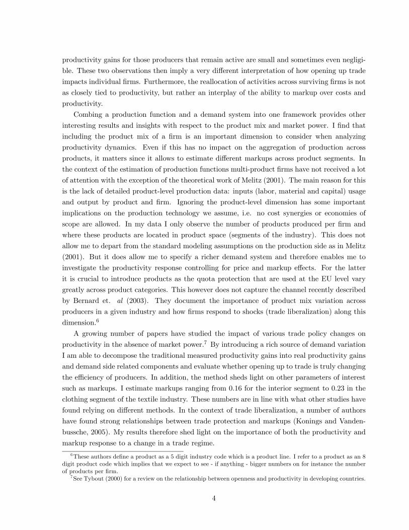
It is straightforward to show the various biases one induces by using miss-measured produc-

tivity in a regression framework. Consider the following regression equation where the interest

lies in δ1 verifying the impact of dit on measured productivity

ωmit = δ0 + δ1dit + zitλ+ εit (18)

where zit captures a vector of control variables and εit is an i.i.d. error term. Using expression

(17) it is straightforward to verify the different sources of correlation that bias the estimate for

δ1∂E(ωmit )

∂dit=

∂E((qIt + ξit)/|η|)∂dit

+∂E(npit)

∂dit+

∂E((η + 1)/η)ωit∂dit

(19)

where the expectation is conditional upon zit. It is clear that impact of dit on productivity (ωit)

is biased and the specific question and data at hand should help to sign the bias introduced by

the various sources. For instance, if dit captures some form of trade liberalization (or protection),

it is expected to have an impact on the industry’s total output and elasticity of demand and

results in a biased estimate for coefficient δ1.

In addition to the various other correlations leading to a biased estimate, the point estimate

of the productivity effect is multiplied by the inverse of the (firm specific) markup. Konings

and Vandenbussche (2005) showed that markups increased significantly during a period of trade

protection after antidumping filings in various industries. The second term in (19) captures the

correlation between the product mix and dit. Bernard, Redding and Schott (2003) suggest that

an important margin along which firms may adjust to increased globalization and other changes

in the competitive structure of markets is through changing their product mix. I will empirically

verify the importance of this bias when evaluating the impact of decreased quota protection in

the Belgian textile industry on estimated productivity in section 5.

4 The Belgian textile industry: Data and institutional details

I now turn to the dataset that I use to apply the methodology suggested above and in a later

stage to analyze the trade liberalization process measured by a significant drop in quota protec-

tion. My data covers firms active in the Belgian textile industry during the period 1994-2002.

The firm-level data are made available by the National Bank of Belgium and the database is

27Harrison (1994) builds on the Hall (1988) methodology to verify the impact of trade reform on productivityand concludes that ”... ignoring the impact of trade liberalization on competition leads to biased estimates in therelationship between trade reform and productivity growth”.

17

commercialized by BvD BELFIRST. The data contains the entire balance sheet of all Belgian

firms that have to report to the tax authorities. In addition to traditional variables - such as

revenue, value added, employment, various capital stock measures, investments, material inputs

- the dataset also provides detailed information on firm entry and exit behavior.

FEBELTEX - the employer’s organization of the Belgian textile industry - reports very de-

tailed product-level information on-line (www.febeltex.be). More precisely, they list Belgian

firms (311) that produce a certain type of textile product. The textile industry can be charac-

terized by 5 different subsectors: i) interior textiles, ii) clothing textiles, iii) technical textiles,

iv) textile finishing and v) spinning. Within each of these subsectors products are listed to-

gether with the name of the firm that produces it. This allows me to construct product-level

information for each firm including the location of those products in the different segments of

the textile industry. In Table A.1 I list the segments and the various product categories.

I match the firms listing product information with the production dataset (BELFIRST) and

I end up with 308 firms for which I observe both firm-level and product-level information.28 The

average size of the firms in the matched dataset is somewhat higher than the full sample, since

mostly bigger firms report the product-level data. Even though I loose some firms due to the

matching of the product and the production datasets, I still cover 70 percent (for the year 2002)

of total employment in the textile industry.29

By adding the rich source of product-level data, it is clear that the industrial classification

codes (NACE BELCODE) are sometimes incomplete as they do not necessarily map into mar-

kets. If one would merely look at firms producing in the NACE BELCODE 17, there would

be some important segments of the industry left out, e.g. the subsector technical textiles also

incorporates firms that produce machinery for textile production and these are not always in

the NACE BELCODE 17 listings. It is therefore important to take these other segments into

the analysis in order to get a complete picture of the industry.

Before I turn to the estimation I report some summary statistics of both the firm-level and

product-level data. In Table 1 summary statistics of the variables used in the analysis are given.

The average firm size is increasing over time (11 percent). In the last column the producer

price index (PPI) is presented. It is interesting to note that since 1996 producer prices fell,

only to recover in 2000. Sales have increased over the sample period, with a drop in 1999.

However, measured in real terms this drop in total sales was even more sharp. Furthermore I

28After matching the two sources of data it turns out that a very small fraction - 17 - of firms included in theFEBELTEX listing are also active in wholesale of specific textiles. I ran all specifications excluding those firmssince they potentially do not actually produce textile and all results are invariant to this.29A downside is that the product-level information (number of products produced, segments and which prod-

ucts) is time invariant and leaves me with a panel of firms active until the end of my sample period. ThereforeI check whether my results are sensitive to this by considering a full unbalanced dataset where I control for theselection bias (exit before 2000) as well as suggested in Olley and Pakes (1996). I can do this as the BELFIRSTdataset provides me with the entire population of textile producers. The results turn out to be very similar asexpected since the correction for the omitted price variable is essentially done in the first stage of the estimationalgorithm. The variation left in capital is not likely to be correlated with the demand variables and therefore Ionly find slightly different estimates on the capital coefficient.

18

also constructed unit prices at a more disaggregated level (3 digit NACEBELCODE) by dividing

the production in value by the quantities produced and the drop in prices over the sample period

is even more prevalent in specific subcategories of the textile industry and quite different across

different subsectors (see Appendix A.).

Together with the average price decrease, the industry as whole experienced a downward

trend in sales at the end of the nineties. The organization of employers, FEBELTEX, suggests

two main reasons for the downward trend in sales. A first reason is a mere decrease in pro-

duction volume, but secondly the downward pressure on prices due to increased competition

has played a very important role. This increased competition stems from both overcapacity

in existing segments and from a higher import pressure from low wage countries, Turkey and

China more specifically.30 Export still plays an important role, accounting for more than 70%

of the total industry’s sales in 2002. A very large fraction of the exports are shipped to other

EU member states and this is important as the quota restrictions are relevant at the EU level.

The composition of exports has changed somewhat, export towards the EU-15 member states

fell back mainly due to the strong position of the euro with respect to the British Pound and the

increased competition from low wage countries. This trend has been almost completely offset

by the increased export towards Central and Eastern Europe. The increased exports are not

only due to an increased demand for textile in these countries, but also due to the lack of local

production in the CEECs.

For each firm in the dataset I observe product-level information. For each firm I know the

number of products produced, which products and in which segment(s) the firm is active. There

are five segments: 1) Interior, 2) Clothing, 3) Technical Textiles, 4) Finishing and 5) Spinning

and Preparing (see Appendix A. for more on the data). In total there are 563 different products,

with 2,990 product-firm observations. On average a firm has about 9 products and 50 percent

of the firms have 3 or fewer products. Furthermore, 75 percent of the firms are active in one

single segment. This information is in itself unique and ties up with a recent series of papers by

Bernard et al. (2003) looking at the importance of differences in product mix across firms where

a 5 digit industry code is the definition of a product. Given I use a less aggregated definition of

a product, it is not surprising that I find a higher average number of products per firm.

Table 2 presents a matrix where each cell denotes the percentage of firms that is active in

both segments. For instance, 4.8 percent of the firms are active in both the Interior and Clothing

segment. The high percentages in the head diagonal reflect that most firms specialize in one

segment, however firms active in the Technical and Finishing segment tend to be less specialized

as they capture applying and supplying segments, respectively. The last row in Table 2 gives

the number of firms active in each segment. Again since firms are active in several segments,

these numbers do not sum up to the number of firms in my sample.

30An example is the filing of three anti-dumping and anti-subsidy cases against sheets import from India andPakistan. Legal actions were also undertaken against illegal copying of products by Chinese producers (AnnualReport of FEBELTEX; 2002). In section 6 I analyze the productivity dynamics during this increased competitionperiod.

19

The same exercise can be done based on the number of products and as shown in Table 3

the concentration into one segment is even more pronounced. The number in each cell denotes

the average (across firms) share of a firm’s products in a given segment in its total number of

products. The table above has to interpreted in the following way: firms that are active in the

Interior segment have (on average) 83.72 percent of all their products in the Interior segment.

The analysis based on the product information reveals even more that firms concentrate their

activity in one segment. However, it is also the case that firms that are active in the Spinning

segment (on average) also have 27.2 percent of their products in the Technical textile segment.

Firms active in any of the segments tend to have quite a large fraction of their products in

Technical textiles, 8.27 to 27.7 percent. Finally the last two rows of Table 3 show the median and

minimum number of products owned by a firm across the different segments. Firms producing

only 2 (or less) products are present in all five segments, but the median varies somewhat

across segments (see Appendix A.1 for a more detailed description of the segments). It is this

additional source of demand variation that I will use to construct segment demand shifters to

estimate segment markups. This is in contrast to Melitz and Levinsohn (2002) who do not

observe any product-level data and have to rely on the number of firms active in the industry

to estimate one markup for the industry.

5 Estimated production and demand parameters

In this section I show how the estimated coefficients of a revenue production function are re-

duced form parameters and that consequently the actual production function coefficients and

the resulting returns to scale parameter are underestimated. Furthermore, I introduce two ad-

ditional sources of demand variation at the product and segment level to control for unobserved

firm-level prices The two sources - segment demand shifters and product dummies - allow for

different product-level demand intercepts and different slopes for the various segments of the

industry. A direct implication is that each firm will face different demand conditions as they

differ in their product mix both within and across segments.

5.1 The estimated coefficients of augmented production function

I compare my results with a few base line specifications: [1] a simple OLS estimation of equation

(2), the Klette and Griliches (1996) specification in levels [2] and differences [3], KG Level and

KG Diff respectively. Furthermore I compare my results with the Olley and Pakes (1996)

estimation technique to correct for the simultaneity bias in specification [4]. In specification [5]

I proxy the unobserved productivity shock by a polynomial in investment and capital and the

omitted price variable is controlled for as suggested by Klette and Griliches (1996). Note that

here I do not consider multi-product firms, I allow for this later when I assume segment specific

demand elasticities.

I replace the industry output QIt by a weighted average of the deflated revenues, i.e. QIt =

20

(P

imsitRit/PIt) where the weights are the market shares. This comes from the observation

that a price index is essentially a weighted average of firm-level prices where weights are market

shares (see Appendix A.2).

Table 4 shows the results for these various specifications. Going from specification [1] to [2] it

is clear that the OLS produces reduced form parameters from a demand and a supply structure.

As expected, the omitted price variable biases the estimates on the inputs downwards and hence

underestimates the scale elasticity. Specification [3] takes care of unobserved heterogeneity by

taking first differences of the production function as in the original Klette and Griliches (1996)

paper and the coefficient on capital goes to zero as expected (see section 1). In specification

[4] we see the impact on the estimates of correcting for the simultaneity bias, i.e. the labor

coefficient is somewhat lower and the capital coefficient is estimated higher as expected. The

omitted price variable bias is not addressed in the Olley and Pakes (1996) framework as they

are only interested in a sales per input productivity measure. Both biases are addressed in

specification [5] and the effect on the estimated coefficients is clear. The correction for the

simultaneity and omitted price variable go in opposite direction and therefore making it hard

to sign the total bias a priori.

The estimate on the capital coefficient does not change much when introducing the demand

shifter as expected since the capital stock at t is predetermined by investments at t−1, however,it is considerably higher than in the Klette and Griliches (1996) approach. The correct estimate

of the scale elasticity (αl+αm+αk) is of most concern in the latter and indeed when correcting for

the demand variation, the estimated scale elasticity goes from 0.9477 in the OLS specification to

1.1709 in theKG specification. The latter specification does not take control for the simultaneity

bias which results in upward bias estimates on the freely chosen variables labor and material.

This is exactly what I find in specification [5], i.e. the implied coefficients on labor drops when

correcting for the simultaneity bias (labor from 0.3338 to 0.3075).31

The estimated coefficient on the industry output variable is highly significant in all specifi-

cations and is a direct estimate of the Lerner index. I also show the implied elasticity of demand

and markup. Moving across the various specifications, the estimate of the average Lerner index

(or the markup) increases as I control for unobserved firm productivity shocks. Moving from

specification [2] to [3] I implicitly assume a time invariant productivity shock which results in

a higher estimated Lerner index (from 0.2185 to 0.2658). In specification [5] productivity is

modelled as a Markov process and no longer assumed to be fixed over time. Controlling for

the unobserved productivity shock leads to a higher estimate of the Lerner index (around 0.30)

as the industry output variable no longer picks up productivity shocks common to all firms as

31Note that here my panel is only restricted to having firms with observations up to the year 2002 in orderto use the product-level information and thus allows for entry within the sample period. However, as mentionedbefore my estimates of the production function are robust to including the full sample of firms. To verify this,I estimate a simple OLS production function on an unbalanced dataset capturing the entire textile sector. Thecapital coefficient obtained in this way is 0.0956 and is very close to my estimate in the matched panel (0.0879),suggesting that the sample of matched firms is not a particular set of firms.

21

picked up by investment and capital.

Finally, an interesting by-product of correcting for the omitted price variable is that I recover

an estimate for the elasticity of demand and for the markup. The implied demand elasticities

are around −3 and the estimated markup is around 1.4.32 These implied estimates are worthdiscussing for several reasons. First of all, this provides us with a a check on the economic

relevance of the demand model I assumed. Secondly, the implicit working assumption in most

empirical work is that η = −∞ and the estimates here provide a direct test of this. Thirdly,

they can be compared to other methods (Hall 1988 and Roeger 1995) that estimate markups

from firm-level production data.

The message to take out of this table is that both the omitted price variable and the simul-

taneity bias are important to correct for, although that the latter bias is somewhat smaller in

my sample. It is clear that this will have an impact on estimated productivity. The estimated

reduced form parameters (β) do not change much when controlling for the omitted price variable

in addition to the simultaneity bias correction since the control is (in these specifications) not

firm specific. However, it has a big impact on the estimated production function parameters (α),

which by itself is important if one is interested in obtaining the correct marginal product of labor

for instance. The industry output variable captures variation over time of total deflated revenue

and as Klette and Griliches (1996) mention therefore potentially picks up industry productivity

growth and changes in factor utilization. If all firms had a shift upwards in their production

frontier, the industry output would pick up this effect and attribute it to a shift in demand

and lead to an overestimation of the scale elasticity. In my approach, the correction for the

unobserved productivity shock should take care of the unobserved industry productivity growth

if there is a common component in the firm specific productivity shocks (ωt).

In the next section I introduce product-level information that allows for firm specific demand

shifters as firms have different product portfolios over the various segments of the industry. Es-

timated productivity will be different due to different estimated parameters (β) and additional

demand controls capturing the shifts in demand for the products of a firm in a given segment

of the industry. The estimated coefficients on the inputs (β) will potentially change as I further

control for unobserved prices and the correlation of inputs with the output price through the

introduction of additional rich demand side variation. The implied production function para-

meters (α) are expected to change as well due to a potentially different reduced form parameter

β and different markup estimates for the various segments.

32Konings, Van Cayseele and Warzynski (2001) use the Hall (1988) method and find a Lerner index of 0.26for the Belgian textile industry, which is well within in the range of my estimates (around 0.30). They have torely on valid instruments to control the for the unobserved productivity shock. A potential solution to overcomethis is a method proposed by Roeger (1995) were essentially the dual problem of Hall (1988) is considered toovercome the problem of the unobserved productivity shock, however one is no longer able to recover an estimatefor productivity.

22

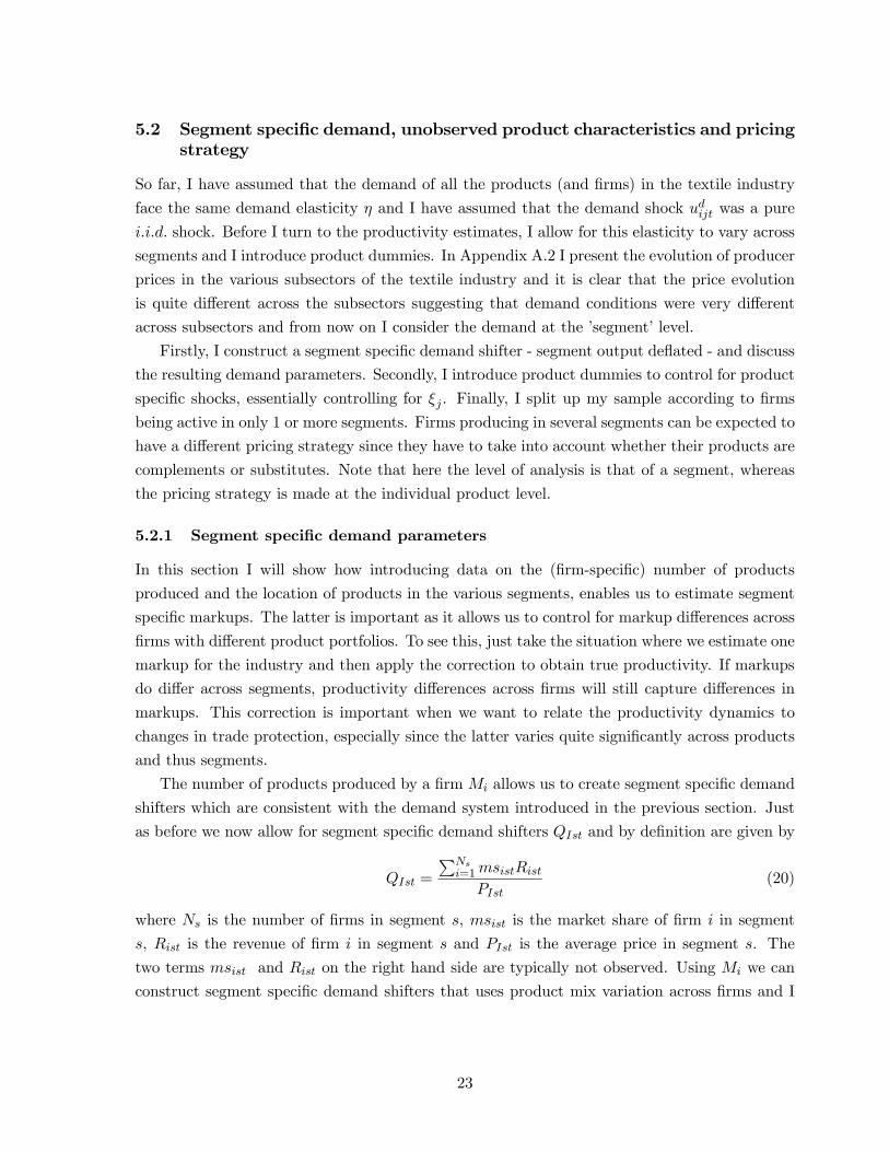
5.2 Segment specific demand, unobserved product characteristics and pricingstrategy

So far, I have assumed that the demand of all the products (and firms) in the textile industry

face the same demand elasticity η and I have assumed that the demand shock udijt was a pure

i.i.d. shock. Before I turn to the productivity estimates, I allow for this elasticity to vary across

segments and I introduce product dummies. In Appendix A.2 I present the evolution of producer

prices in the various subsectors of the textile industry and it is clear that the price evolution

is quite different across the subsectors suggesting that demand conditions were very different

across subsectors and from now on I consider the demand at the ’segment’ level.

Firstly, I construct a segment specific demand shifter - segment output deflated - and discuss

the resulting demand parameters. Secondly, I introduce product dummies to control for product

specific shocks, essentially controlling for ξj . Finally, I split up my sample according to firms

being active in only 1 or more segments. Firms producing in several segments can be expected to

have a different pricing strategy since they have to take into account whether their products are

complements or substitutes. Note that here the level of analysis is that of a segment, whereas

the pricing strategy is made at the individual product level.

5.2.1 Segment specific demand parameters

In this section I will show how introducing data on the (firm-specific) number of products

produced and the location of products in the various segments, enables us to estimate segment

specific markups. The latter is important as it allows us to control for markup differences across

firms with different product portfolios. To see this, just take the situation where we estimate one

markup for the industry and then apply the correction to obtain true productivity. If markups

do differ across segments, productivity differences across firms will still capture differences in

markups. This correction is important when we want to relate the productivity dynamics to

changes in trade protection, especially since the latter varies quite significantly across products

and thus segments.

The number of products produced by a firm Mi allows us to create segment specific demand

shifters which are consistent with the demand system introduced in the previous section. Just

as before we now allow for segment specific demand shifters QIst and by definition are given by

QIst =

PNsi=1msistRist

PIst(20)

where Ns is the number of firms in segment s, msist is the market share of firm i in segment

s, Rist is the revenue of firm i in segment s and PIst is the average price in segment s. The

two terms msist and Rist on the right hand side are typically not observed. Using Mi we can

construct segment specific demand shifters that uses product mix variation across firms and I

23

use Mi to compute

Rist = RitMis

Mi(21)

msist =RistPiRist

(22)

whereMis andMi are the number of products firm i has in in segment s and in total, respectively.

Now that we have segment output (QIst) it suffices to weigh across segments according to

Sis =MisMi

to obtain a firm-specific total demand shifter. All firms now (potentially) face 5

different (segments) demand shifters and the product-mix variance in addition to the segment

demand shifters are used to identify the segment markups βηs . The latter are - just like in

the case of the single markup - the coefficients on the 5 terms ln(SisQIst) in the augmented

production function.33

In this way I weigh the various demand shifters by firm across segments according to how

important a segment is for a firm’s total revenue. This firm-specific importance is measured

by the share of the number of products in a given segment. For example a firm with 9 out

of its 10 products located in segment 1 will get a weight of 0.9 on demand shocks specific for

segment 1. This additional source of variation across firms (using the firm-specific product mix)

is then used to identify segment specific markups. It is clear that this approach might introduce

some measurement error by forcing firm-segment revenues to be proportional to the share of

the number of products sold in a given segment. However, as long as the proportionality is not

violated in some systematic way across products and segments, it is not expected to bias my

estimates in any specific way.

In this way the demand parameter is freed up to be segment-specific s by interacting the

segment demand shifter (segment output) with the segment share variable Sis.34 This implies

that I will now recover markups for s = {1 (Interior), 2 (Clothing), 3 (Technical), 4 (Finishing),5 (Spinning and Preparing)}. Note that the demand elasticity is now identified using firm

specific variation as the share variable is firm specific and Tables 3 and 4 show the variation in

the product mix of firms across segments.35

I now turn back to the general setup of the paper and denote qist = ln(SisQIst) which

captures the segment specific demand shifter weighted by the number of products a firm has in

a given segment . The augmented production function I estimate is clearly extended by allowing

33Note that here I have constrained the number of products per firm Mi to be time-invariant as in my dataset.Obviously when the product mix is observed at each point in time this introduces another rich source of identifyingvariation.34 I have also estimated demand parameters one level deeper, see Appendix A.1 for the structure of the segments.

This leads to a model with 51 different demand elasticities and identification is somewhat harder as the numberof observations for some of the products is insufficient. However, for a set of subsegments I recover significant andmeaningful estimates for markups.35As mentioned before, I do not observe the change of the product mix over time. It is reassuring, however,

that based on the US Census data (Bernard et al. 2003) firms only add or drop about 1 product over a five yearperiod, or less than 2 products over a nine year period which corresponds to my sample length (1994-2002). Tothe extend that this variation is not picked up by the proxy for ωi, it potentially biases the input coefficients.

24

η to vary by segment s

erit = β0 + βllit + βmmit +5X

s=1

βηsqist + βnpnpit + φt(iit, kit) + uit (23)

I present the estimated coefficients βηs and the distribution of the estimated demand parameter

in Table 5. One can immediately read of the implied demand parameters for the various segments

in the textile industry for those firms having all their products in one segment (Sit = 1).

Introducing multi-product firms in this framework explicitly implies a correction for the

number of products produced. As mentioned before, since I do not observe the product specific

inputs at the firm level, I have assumed that the product specific input levels are proportional

to the total firm input, where the proportion is given by the number of products produced

(lnMi = npi). The coefficient on this extra term is negative and highly significant, however, it

is hard to interpret especially in the context of the control function (ωit = h(iit, kit)) as it is quite

plausible that the investment decision of a firm depends on the number of products produced.

The first row in Table 5 shows the estimated coefficients implying significantly different

demand parameters for the various segments. I also include the implied demand parameters

relevant for firms having all their products in a given segment. For instance, firms having all

their products in the segment Interior face a demand elasticity of −5.3. In panel B of table5 I use the firm specific information on the relative concentration (Sis) and this results in a

firm specific elasticity of demand and markup which are in fact weighted averages over the

relevant segment parameters. I stress that this comes from the fact that firms have multiple

products across different segments and therefore the relevant demand condition is different for

every firm.36

5.2.2 Unobserved product characteristics

I now introduce product dummies to control for product specific unobserved demand shocks (ξj).

Note that in my empirical implementation the unobserved demand shock - which is potentially

correlated with the other demand variables (segment output) - is now time invariant and only

product specific (ξj) due to the lack of time-varying product-mix information (as opposed to

being firm and time specific in the theoretical setup).

In terms of section 3.2 the product dummies proxy for the unobserved demand shocks - that

are product specific and potentially impacts the investment decision. I assume time invariant

unobserved product characteristics and there are 563 products (K) in total (and a firm produces

9 of these on average) which serve as additional controls in the first stage regression (24). The

product dummies are captured by PRODik where PRODik is a dummy variable being 1 if firm

i has product k. The variation across firms in terms of their product mix allows me to identify

the K product fixed effects and they have a specific economic interpretation.

36The same is true for the estimated production function coefficients, since they are obtained by correcting forthe degree of production differentiation which is firm specific (ηi).

25

Note that I introduce the product dummies motivating the need to correct for product

specific demand shocks such as unobserved quality. However, they will also capture variation

related to the production side and those two types of variations are not separable.37 The

identifying assumption for recovering an estimate on the capital coefficient is that productivity

and the unobserved demand shock are independent. However, using the product dummies in

the proxy for productivity, the identifying assumption becomes less strong, i.e. I filter out

time invariant product unobservables. Note that in the standard approach for identifying the

production coefficients, demand variation is not filtered out, both observed and unobserved.

Here I allow for product unobservables and demand shocks to impact investment decisions, on

top of proxying for the demand shocks by segment output and product dummies. Note that I

assume that ξijt = ξj and I only control for product time invariant demand shocks as opposed

to time varying firm-product specific demand shocks.

erit = β0+βllit+βm mit+5X

s=1

βηsqstSis+βnpnpi+eφt (iit, kit, PRODi1, ..., PRODiK)+uit (24)

In Table 5 I show that the demand parameters do not change too much as expected, as well

as the production related coefficients. However, the point estimates are more precise and 62 out

of the 652 products are estimated significantly different from the reference product confirming

the importance of controlling for time invariant product characteristics. As mentioned above the

interpretation of these coefficients is somewhat harder as the product dummies are introduced to

proxy for unobserved demand shocks, however, they will also pick up product-specific production

related differences. As stressed before, all these extra controls come into play if the interest lies

in getting an estimate on productivity taking out demand related variation.

In terms of economic interpretation, Table 5 suggests that firms operating in the Finishing

segment (only) face less elastic demand. The high elastic demand segments are Interior and

Spinning capturing products - like linen, yarns, wool and cotton - facing high competition from

low wage countries.38 In Appendix A.1 I relate these demand parameters to changes in output

prices at more disaggregated level and I find that indeed in those sectors with relative high

elastic demand, output prices have fallen considerably over the sample period.

5.2.3 Single versus multi-product firms

So far I have assumed that the pricing strategy of firms is the same whether it produces one or

more products, or whether it is active in one or more segments. Remember that the revenue37 I introduce the product dummies without interactions with the polynomial terms in investment and capital

since that would blow up the number of estimated coefficients by K. This then coincides with assuming that thequality unobservable does not enter the investment policy function in the first stage and just correcting for thedemand unobservable. However, it matters for the second stage, i.e. this variation is now not subtracted fromdeflated sales (r) like the variable inputs. This would imply that the time invariant product dummies would proxythe unobserved demand shock completely. Therefore, the resulting productivity will still capture time variantdemand shocks - say improved product quality.38 Increased international competition in the Interior and Spinning segments is documented in section 6 where

quota protection is discussed.

26

observed at the firm-level is the sum over the different product revenues. Firms that have

products in different segments are expected to set prices differently since they have to take

into account the degree of complementarity between the different goods produced. I relax this

by simply splitting my sample according to the number of segments a firm is active in. The

underlying model of price setting and markups can be seen as a special case where own and

cross elasticities of demand are restricted to be the same within a segment.

In the third row of Table 5 I present the estimated demand parameters for firms active in

only 1 segment and for those active in at least 2. As expected the estimated demand elasticities

for the entire sample are in between both. Firms producing products in different segments face

a more elastic (total) demand since a price increase of one of their product also impacts the

demand for their other products in other segments.39 This is not the case for firms producing

only in 1 segment, leading to lower estimated demand elasticities. It is clear that the modeling

approach here does allow for various price setting strategies and different demand structures.

From the above it is clear that productivity estimates are biased in the presence of imperfect

competitive markets and ignoring the underlying product space when considering firm-level

variables. It is clear that the data at hand and the research question will dictate the importance

of the various components captured by traditional productivity estimates. In the next section I

analyze the productivity gains from the trade liberalization in the Belgian textile industry and I

compare my results with the standard productivity estimates, which are in fact sales per input

measures and not necessarily lead to the same conclusions.

6 Trade liberalization and productivity gains

In this section I introduce product-level quota restrictions as additional controls for the un-

observed firm-level price variable in the demand system and consequently in the augmented

production function. In section 5 I showed that the industry output and segment output vari-

ables were highly significant, however, they implied rather high markups and in turn relatively

high returns to scale point estimates. Including the quota restriction variable is expected to

lead to lower estimates on the demand shifters QIst if anything as firms protected by quota are

expected to have higher market share - if anything - and produce more. I will correct for the

potential upward bias in the Lerner index. In addition the quota variable will control for addi-

tional variation in unobserved firm-level prices as producers are expected to be able to set higher

prices if import is restricted even more so since quota tend to apply on suppliers with lower costs

of production (wages). I model the quota restriction variable as an additional residual demand

shock in the demand system and it will impact each firm demand intercept differently according

to the firm’s product mix.

39Note that now the implied demand elasticities are given by the weighted sum over the various segments afirm is active in, where weights are the fraction of the number of products in a segment in the total number ofproducts owned.

27

First I introduce the quota data and discuss how it relates to the firm-level data. Secondly, I

introduce the quota restriction measure into the augmented production function. The resulting

estimated productivity is then used to verify to what extent that abolishing the quota on imports

has contributed to within-firm productivity gains in the Belgian textile industry and how results

using standard techniques to estimate productivity differ from the methodology suggested in

this paper. In contrast to within-firm productivity changes, aggregate industry productivity can

increase by the mere exit of lower productivity firms and/or the reallocation of market share

towards more productive firms.40 As shown in Syverson (2004), demand shocks might in turn

impact the aggregate productivity distribution.

6.1 The quota data: raw patterns and a measure for trade liberalization

The quota data comes straight from the SIGL database constructed by the European Commission

(2003) and is publicly available on-line (http://sigl.cec.eu.int/). Note that this data is at the EU

level since Belgium has no national wide trade policy and so quota at the EU level are the relevant

quota faced by Belgian producers. This database covers the period 1993-2003 and reports all

products holding a quota. For each product the following data is available: the supplying

country, product, year, quota level, working level, licensed quantity and quantity actually used

by the supplying country.41 From this I constructed a database listing product-country-year

specific information on quota relevant for the EU market.

Before I turn to the construction of a variable capturing the quota restriction relevant at

the firm level, I present the raw quota data as it shows the drastic changes that occurred in

trade protection during my sample period 1994-2002. In addition to observing whether a given

product is protected by a quota, the level of allowed import quantities measured in kilograms

(kg) or number of pieces - depending on the product category - is provided. In total there are

182 product categories and 56 supplying countries, where at least one quota on a product from

a supplier country in a given year applies. In terms of constructing a trade liberalization or

protection measure various dimensions have to be considered.

Given the structure of the demand system and how the quota restriction will impact firm-

level demand I create a composite variable that measures the extent to which a firm is protected

(across its products). A first and most straightforward measure is a dummy variable that is 1 if

a quota protection applies for a certain product category g on imports from country e in year t

(qregt) and switches to zero when the quota no longer applies. However, increasing the quota

levels is also consistent with opening up to trade and thus both dimensions are important to

look at. Table 6 below shows the number of quota that apply for the sample period 1994-2002.

40 It is clear that decompositions of aggregate industry productivity using biased measures of firm-level produc-tivity will provide different answers as to how important net entry, reallocation and within productivity growthare. In fact given the framework suggested here, it is easy to show how we over- (under) estimate the variouscomponents of aggregate productivity. Under the empirical relevant scenario that entrants charge lower prices, itis clear that the importance of entry is underestimated since ωMit = ωit + (pit − pIt).41Appendix A.4 describes the quota data in more detail and provides two cases on how quota protection changed.

28

In addition I provide the average quota levels split up in kilograms and number of pieces, both

expressed in millions.

It is clear from the second column that the number of quota restrictions have decreased

dramatically over the sample period. By 2002 the number of quota fell by 54 percent over a

nine year period and these numbers refer to the number of product-supplier restricted imports.

Columns 3 to 6 present the evolution by unit of measurement and the same evolution emerges:

the average quota level increased with 72 and 44 percent for products measured in kilograms

and number of pieces, respectively. Both the enormous drop in the number of quota and the

increase in the quota levels of existing quota, points to a period of significant trade liberalization

in the EU textile industry. It is essentially this additional source of demand variation I will use

to identify the demand parameters in the augmented production function and verify how this

gradual opening up to foreign textile products has impacted firm-level productivity.

As mentioned above the product classifications in the quota data are different from the firm-

level activity information and have to be aggregated to the firm-level revenue and input data.

The average quota restriction (qr) that applies for a given product g is given by

qrgt =Xe

aetqregt (25)

where aet is the weight of supplier e in period t. This measure is zero if no single quota applies to

imports of product g from any of the supplying countries at a given time, and one if it holds for

all supplying countries. A final step is to relate the quota restriction measure to the information

of the firm revenue and production data. The 182 different quota product categories map into

390 different 8 digit product codes. The latter correspond to 23 (l) different 4 digit industry

classifications (equivalent to the 5 digit SIC level in the US) allowing me to relate the quota

restriction variable to the firm-level variables. Aggregating over the different product categories

leaves me with a quota measure of a given 4 digit industry code. I consider the average across

products within an industry l (qrit) where a firm i is active in as given by (26).

qrit =1

Ngt

Xg∈l(i)

qrgt (26)

In Figure 1 I show the evolution of the quota restriction variable given by (26) split up by

segment. Again the same picture emerges, in all segments the average quota restriction has

gone down considerably over the sample period, however, there are some differences across the

various segments and it is this variation that will help to estimate the segment specific demand

elasticities.

The construction of the quota restriction measures provides me with an additional control

for the unobserved price variable and it is assumed to enter the demand system (4) as part of the

residual demand shock in the demand system in addition to the pure i.i.d. component udit and

unobserved demand shocks ξit. This implies that it is assumed to be independent (conditional

on the other controls) of the input and investment choices.

29

6.2 Introducing quota restrictions in the demand system

I now introduce the average quota restriction qrit in the demand system where I now have the

following expression.

Qit = QIt

µPitPIt

¶η

exp(udit + ξit + qrit) (27)

The interpretation of this model is to estimate the elasticity of substitution (demand) that is

consistent with international competition. It implies that the intercept for each firm is allowed

to differ according to the protection of its products.42 I allow for segment specific demand

elasticities and multi-product firms and I control for time invariant unobserved product effects

using product dummies. This leads to the following augmented production function (28)

erit = β0 + βllit + βmmit +5X

s=1

βηsqist + βqrqrit + βnpnpi

+φt(iit, kit) +KXk=1

λkPRODik + uit (28)

where the term βqrqrit captures the quota measures.43 Before I present the estimated coefficients,

I note that introducing the quota restriction information helps estimating the βηs and potentially

the production function parameters. Table 7 presents the estimated Lerner indices (βηs) and

compares them with the specification where the extra demand variation captured by the quota

restriction is not included. I also recover product specific estimates and about 20 products

are estimated significantly different from their respective segment average (see Appendix A.3).

These can be interpreted as the product of segment specific Lerner indices and time invariant

product shocks ξj under the assumption that the investment decision does not depend on the

unobserved demand shock. This is the assumption implicitly made in expression (28) as they

do no longer enter in the control function φt(iit, kit).

The last 4 rows show the estimated production coefficients and the implied returns to scale.

The estimate on the quota restriction variable immediately provides information on how standard

estimated productivity estimates incorporate demand shifters.44 We could immediately verify

42 I have also estimate a change in the slope of the demand curve (elasticity). The identification is somewhatharder as firms can be active in different segments experiencing different changes in the protection, however, theresults are invariant.43A well documented problem of using trade liberalization or protection measures in a regression framework

is that they are potentially endogenous as firms might lobby for protection. In order to verify whether in mysample producers of certain product categories were able to keep higher level of protection, I ran a regression ofqrge2003 on qrge1993 (N = 1, 097) finding a strong negative relation which suggests that protection in all productcategories decreased over time. In addition, when analyzing the productivity effects I include product category (l)dummies controlling for (time invariant) differences in lobbying-for-protection activities across producers activein different product categories.44All the results are based on unweighted averages. I have also experimented using the quota levels to construct

the weights. These would capture the importance of a given quota protection in the overall import restrictionand the extent to which import demand for a given product can be substituted away to another supplier. Due tothe different unit of measurement in the levels, the interpretation of a change in qr is less clear.

30

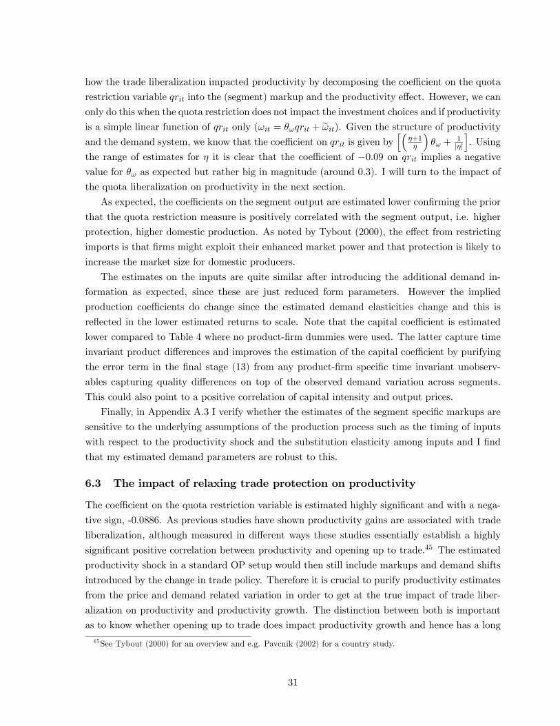
how the trade liberalization impacted productivity by decomposing the coefficient on the quota

restriction variable qrit into the (segment) markup and the productivity effect. However, we can

only do this when the quota restriction does not impact the investment choices and if productivity

is a simple linear function of qrit only (ωit = θωqrit + eωit). Given the structure of productivityand the demand system, we know that the coefficient on qrit is given by

h³η+1η

´θω +

1|η|

i. Using

the range of estimates for η it is clear that the coefficient of −0.09 on qrit implies a negative

value for θω as expected but rather big in magnitude (around 0.3). I will turn to the impact of

the quota liberalization on productivity in the next section.

As expected, the coefficients on the segment output are estimated lower confirming the prior

that the quota restriction measure is positively correlated with the segment output, i.e. higher

protection, higher domestic production. As noted by Tybout (2000), the effect from restricting

imports is that firms might exploit their enhanced market power and that protection is likely to

increase the market size for domestic producers.

The estimates on the inputs are quite similar after introducing the additional demand in-

formation as expected, since these are just reduced form parameters. However the implied

production coefficients do change since the estimated demand elasticities change and this is

reflected in the lower estimated returns to scale. Note that the capital coefficient is estimated

lower compared to Table 4 where no product-firm dummies were used. The latter capture time

invariant product differences and improves the estimation of the capital coefficient by purifying

the error term in the final stage (13) from any product-firm specific time invariant unobserv-

ables capturing quality differences on top of the observed demand variation across segments.

This could also point to a positive correlation of capital intensity and output prices.

Finally, in Appendix A.3 I verify whether the estimates of the segment specific markups are

sensitive to the underlying assumptions of the production process such as the timing of inputs

with respect to the productivity shock and the substitution elasticity among inputs and I find

that my estimated demand parameters are robust to this.

6.3 The impact of relaxing trade protection on productivity

The coefficient on the quota restriction variable is estimated highly significant and with a nega-

tive sign, -0.0886. As previous studies have shown productivity gains are associated with trade

liberalization, although measured in different ways these studies essentially establish a highly

significant positive correlation between productivity and opening up to trade.45 The estimated

productivity shock in a standard OP setup would then still include markups and demand shifts

introduced by the change in trade policy. Therefore it is crucial to purify productivity estimates

from the price and demand related variation in order to get at the true impact of trade liber-

alization on productivity and productivity growth. The distinction between both is important

as to know whether opening up to trade does impact productivity growth and hence has a long

45See Tybout (2000) for an overview and e.g. Pavcnik (2002) for a country study.

31

run impact on the efficiency of an economy.

The interpretation in my specification is somewhat more complicated. To the extent that

the polynomial in capital and investment picks up the unobserved productivity shock, the quota

restriction variable picks up demand shocks. However, it is clear that it will also pick up

variation related to true productivity that is not controlled for by the polynomial in investment

and capital. It is exactly the relation between productivity and the trade liberalization measure

that is of interest.

In order to verify the extent to which trade liberalization - measured by a decrease in quota

restrictions - has impacted the productivity of Belgian textile producers I follow the standard 2

stage approach and show how the results change when using my corrected productivity estimates.

I consider the following regression

bωit = δ0 + δ1qrit + δ2nqrit + εit (29)

where bωit refers to the estimated productivity and I will consider various versions of (29). Inall regressions I include quota product classification dummies (23 categories) capturing time

invariant productivity (growth) differences among categories. Table 8 presents the estimates of

δ1 under various specifications.

Before I turn to each specification, it is clear that - across all specifications - using the stan-

dard OP productivity estimate leads to an overestimation of the impact of trade liberalization.46

Note that a decrease in the quota restriction variable corresponds with less quota protection or

opening up of trade. So a negative coefficient implies productivity gains from relaxing quota

restrictions. In all specifications the sign is negative and highly significant and the interpretation

of the coefficient is the productivity gain for abolishing quota on all products from all countries.

Specification I is the level regression and implies a 6.37 percent higher productivity for

firms not protected by a single quota and using OP the estimate is much higher, 10.68 percent.

Given the Markov assumption of productivity in the estimation algorithm and knowing that

firm productivity estimates are highly persistent over time, specification II introduces lagged

productivity as a regressor. The impact of the quota restriction variable is estimated more precise

and somewhat lower. In specification III and IV , I run the regression in growth rates revealing

the same pattern as in specification I. In specification IV , however, I include lagged levels of

the quota restriction variable. Controlling for the lagged levels of the quota restriction measure

leads to a higher point estimate on δ1, showing that the impact of relaxing quota restrictions

on productivity depends on the initial level of the quota. If the quota protection was initially

low, there is not much impact on productivity. Specification V considers long differences (3 year

period) and the results are robust to this, although estimated somewhat less precise due to the

significant drop in observations.

46Using the estimates one can derive that the segments with a relative high level of protection have highermarkups as expected (e.g. Tybout 2000). This - together with the scaled point estimate - leads to a biasedestimate of the effect of relaxing quota protection on standard estimated productivity (OP).

32

In order to recover an estimate of the elasticity of productivity with respect to quota restric-

tions, I evaluate this at the mean (of the change in quota restriction) by segment. Table 9 shows

the impact of a 10 percent decrease in the quota restriction measure on productivity for the

various segments and it further compares my results with those relying on the OP productivity

estimates. A 10 percent decrease in the quota restriction measure can come about by products

being no longer protected from all or some supplying countries.47

As established in the previous table trade liberalization leads to higher productivity, how-

ever, there are some differences across segments. A 10 percent decrease in my quota restriction

measure leads only to a 1.6 percent higher productivity in the Finishing segment, as opposed to

a 4.37 percent increase in the Interior segment. This result is what one would expect given the

different paths of the quota restriction variable by segment as shown in Figure 1. The Finishing

segment started out with a relatively low level of protection in 1994 (0.3) and stays rather flat

after 1996. The other segments - with higher estimated elasticities - had much higher levels

of protection initially, e.g. the Interior segment was highly protected (qr = 0.85) in 1994 and

by 2002 protection was significantly lower (qr = 0.3). It is clear that the productivity gains

are much smaller (more than halved) and this is what one would expect for firms operating

in an advanced economy, as opposed to firms active in more developing regions. The results

show that decomposing the residual from a sales generating production function into productiv-

ity and demand related factors, is important to evaluate the impact of trade liberalization on

productivity.

Furthermore in Table 9, I present the elasticities evaluated at the mean of the change in

the quota restriction for two different periods, 1994-1997 and 1998-2002. The first period is

characterized by a sharper fall in the quota protection (see Table 9) and therefore leads to

higher estimated elasticities. The sharp fall of the number of quota in the period 1994-1997 is

consistent with the process of the preparation of EU enlargement towards Central and Eastern

Europe (CEE). By the year 1998 almost all trade barriers between the EU and the candidate

countries of CEE were abolished as part of the Europe Agreements (EC 2005). The Europe

Agreements were setup to establish free trade in industrial products over a gradual, transition

period. This implied that industrial products from the associated countries (mostly CEE) have

had virtually free access to the EU since the beginning of 1995 with restrictions in only a

few sectors, such as agriculture and textiles. However, even in the last period (1998-2002)

the productivity gains are still estimated around 3 percent with the exception of the Finishing

segment which had a relatively low level of quota protection throughout the sample period.

Finally, as mentioned before another channel through which the EU trade policy relaxed

quota restrictions is by increasing the level of existing quota for a set of supplying countries.

In order to verify the impact of this on productivity I consider only those industry categories

(4 digit NACE) that have some form of protection, i.e. where I observe a positive level of

47The average quota restriction measure is 0.43 and the average change in this measure is -0.05, which is around10 percent.

33

protection and the unit of measurement of a quota level is constant within a given industry code

(23 categories). This dimension of opening up to trade has been the predominant strategy for

the EU when it comes to imports from outside CEE and other new EU member states and not

as much through abolishing quota. In Table 10 I list the supplying countries where relaxing

import restrictions mainly occurred through higher levels of quota. I report the increase in the

average level per quota during my sample period 1994-2002. The countries listed have gained

access to the EU textiles market under a significant increase of quota levels.

For instance the average quota level on textile products from Pakistan has more than doubled

over a nine year period (129 and 144 percent depending on product category). This process is

not captured by the quota restriction variable that picks up whenever a quota on a given product

from a supplying country is abolished.

In order to verify the impact of increased quota levels - in addition to the abolishment of

quota - I include a variable that measures the total level of quota (in logs) in a given industry in

the regression framework of specification II. Specification V I in Table 10 shows the results of

including the level variable. The quota restriction variable has a negative sign as before and the

coefficient on the level variable is estimated with a positive sign: an increase in the level of quota

is consistent with increased competition from foreign textiles products and has a positive effect

on productivity. The point estimate is an elasticity and implies that if quota levels increase by

10 percent that productivity increases with 1.9 percent.

The simultaneous abolishment of quota protection and the increase in the quota levels are

associated with higher productivity of Belgian textile producers. Productivity gains were higher

for firms active in segments which initially were highly protected as they had to restructure

more in order to face the increased competition from non-EU textile producers. However, the

magnitude of the productivity gains are fairly small compared to those obtained with standard

techniques. As mentioned before, the results presented in Table 10 can be interpreted as a

decomposition of measured productivity gains from relaxing trade protection into true produc-

tivity gains and demand shocks. Here, I find that around 50 percent is only picking up actual

productivity gains.

My results suggest that the channel through which trade liberalization impacts productivity

is mostly by cutting off the inefficient producers from the productivity distribution and therefore

increases the average productivity of the industry. However, the (within-firm) productivity

gains for those producers that remain active are small and sometimes even negligible. These

two observations then imply a very different interpretation of how opening up trade impacts

individual firms. Furthermore, the reallocation of activities across surviving firms is not as

closely tied to productivity, but rather an interplay of the ability to markup over costs and

productivity.

34

7 Conclusion

In this paper I suggest a method to correct for the omitted price variable in the estimation

of productivity. I have introduced a simple demand side and I explicitly allow firms to have

multiple products. I introduce a simple aggregation from product space into firm space and

derive a straightforward estimation strategy. I show that measured productivity increases need

not to reflect actual productivity increase. This casts some doubt on the recent empirical

findings that link changes in the operating environment - such as trade protection - on firm-

level productivity (growth) in a two-stage approach. I illustrate this methodology by analyzing

productivity in the Belgian textile industry using an unique dataset that in addition to firm-level

data has product-level information. Adding extra product-level information to the plant-level

data appears to be a successful first step in separating out demand variation and product mix

from estimated productivity.

The results here are obtained using a tractable and fairly standard demand system. The

extent to which the results established in this paper are robust to using a richer demand system

is ultimately an empirical question. However, it is clear that independent of a specific demand

system, the resulting productivity estimates do change quite drastically if one is no longer

ignorant about the product level and the degree of product differentiation in an industry, and

how these factors differ over time and firms.

I analyze the impact of trade liberalization on firm performance using the method developed

in this paper. Trade liberalization is measured by the abolishment of quota restricted imports

and by increased levels of maintained quota. The quota restriction measures serve as additional

variables to control for the unobserved price and the resulting estimates for productivity are

therefore further purified from demand variation. While I find positive significant productivity

gains from relaxing quota restrictions, the effects are estimated considerably lower than using

standard productivity estimates. The latter still capture price and markup variation (across

product segments and time) which are correlated with the change in demand conditions due to

a change of trade policy, leading to an overestimation of productivity gains from opening up to

trade.

35

Appendix A: The Belgian textile industry and the quota dataset

A.1 The Belgian textile industry:

I present the structure of the different segments, sub-segments and the products in mydataset in Table A.1. The different levels are important to structure the regressions and serveas additional sources of variation to identify demand parameters. The number in parenthesesindicates the number of subsegments within a given segment whereas the last row indicates thenumber of products within a given segment. I also estimated demand elasticities at the level ofthe subsegments, i.e. 52 different parameters.

Table A.1.: Segment Structure: Number of Subsegments and Products per Segment

Interior (9) Clothing (18)Fabrics Knitwear

Bed linen Accessories AccessoriesCarpets Baby clothes & children’s Babies’ wear

Kitchen linen Men’s wear BathMattress ticking Nightwear & underclothing Children’s wearTable linen Others Fabrics for ...

Terry toweling articles Rain-, sportswear & leisure ... NightwearTrimming Women’s wear ... Outerwear

Upholstery & furnishing fabr. Workwear & protective suits ... SportswearWallcoverings Stockings- tights- socks

Underwear19 61 36

Technical (9) Finishing (7) Spinning (9)Agrotech Carpeting Blended aramid, polyamid or polyacrylicBuildtech Knitted fabrics Blended artificial yarnsGeotech Material before spinning Blended cotton or linen yarnsIndutech NonWoven Blended polyester yarnsMedtech Woven fabrics Blended polypropylene or chlorofibre yarnsMobiltech Yarns Blended yarnsPacktech Specialities Filament YarnsProtech Spun Yarns (> 85% of 1 fibre)Sporttech Synthetic Fibres231 132 84

36

A.2. Producer prices and demand elasticity

As mentioned in the text a producer price index is obtained by taking a weighted aver-age over a representative number of products within an industry, where weights are based onsales (market shares). In the case of Belgium the National Institute of Statistics (NIS) gathersmonthly information of market relevant prices (including discounts if available) of around 2,700representative products (an 8 digit classification - PRODCOM - where the first 4 are indicat-ing the NACEBELCODE). The index is constructed by using the most recent market share asweights based on sales reported in the official tax filings of the relevant companies. The relevantprices take into account both domestic and foreign markets and for some industries both indicesare reported. I present unit prices at the 3 digit NACEBELCODE (equivalent to 4/5 digit ISICcode). I constructed these by dividing total value of production in a given subcategory by thequantity produced. Table A2 gives the PPI for the various subcategories with 1994 as base yearexcept for the 175 category (Other textile products, mainly carpets). I do not use these to de-flate firm-level revenues since I have no information in which category (ies) a firm is active sincethe product classification cannot be uniquely mapped into the NACEBELCODE and firms areactive in various subcategories. The codes have the following description: 171 : Preparation andspinning of textile fibres, 172 : Textile weaving, 173 : Finishing of textiles, 174 :.Manufactureof made-up textile articles, except apparel, 175 : Manufacture of other textiles (carpets, ropes,...), 176 : Manufacture of knitted and crocheted fabrics and 177 : Manufacture of knitted andcrocheted articles.

Table A.2.: Producer Prices (Unit Prices) at Disaggregated Level

171 172 173 174 175 176 1771994 100 100 100 100 - 100 1001995 99.4 96.7 110.4 111.0 - 100.9 100.71996 100.9 94.5 101.1 117.9 100 103.4 94.81997 103.7 94.5 101.3 108.5 99.2 93.9 97.51998 102.8 96.0 108.0 117.6 101.5 93.3 97.61999 95.0 95.8 100.6 118.2 99.6 94.8 92.92000 94.3 94.6 119.3 106.2 102.0 84.1 95.52001 96.7 93.2 108.4 107.7 104.1 86.9 101.32002 97.3 94.2 110.7 103.1 107.2 85.8 106.1

demand elasticity -5.4675 -3.0628 -3.0628 n.a. n.a. -3.6470

Several observations are important to note. Firstly, there is considerable variation acrosssubcategories of the textiles industry in terms of price changes over the period 1994-2002. Thesector Manufacture of knitted and crocheted fabrics (176) has experienced a severe drop inoutput prices (14.2 percent) over the sample period, whereas the output prices in the Finishingof Textiles (173) has increased with more than 10 percent. Secondly, the evolution in the varioussubcategories is not smooth, periods of price increases are followed by decreases and the otherway around. Thirdly, most of the price decreases occur at the end of the nineties when importsfrom Central and Eastern Europe were no longer quota restricted as agreed in the EuropeAgreements. It is interesting to note that the segment (Spinning) with the most elastic demand(-5.3135) has indeed experienced a negative price evolution (2.7 percent). The latter segmentalso captures weaving activities which in turn also experienced a price decrease (5.8 percent).The segment (Finishing) with the least elastic demand (-3.2051) has had a sharp increase in itsoutput prices (10.7 percent). The estimated demand elasticities from Table 5 are given in thelast row for those subcategories I could map into segments.

37

A.3. Unobserved demand shocks and estimating production function

Formally, I relax the assumption that investment only depends on the capital stock andthe unobserved productivity shock. I now have two unobservables (ωit, ξit) and the investmentfunction is now iit = it(kit, ωit, ξit). The demand unobservable ξit is assumed to follow a Markovprocess that is independent of the productivity process. We now need a second control sit - sayadvertisement expenditures - to proxy the unobservable in order to control for the productivityshock. I denote the bivariate policy function determining (iit, sit) as Υ(.) and assume it is abijection in (ωit, ξit) conditional on the capital stock kitµ

iitsit

¶= Υt(kit, ωit, ξit) (A.1)

As Ackerberg and Pakes (2005) show this allows us to invert and rewrite the unobservableproductivity as a function of the controls in the following way

eωit = Υ−1t (kit, iit, sit) (A.2)

The revenue generating production function is as before and the first stage of the estimationalgorithm now looks as follows

erit = β0 + βllit + βm mit + βkkit + βηqIt +Υ−1t (kit, iit, sit) + uit

= β0 + βllit + βm mit + βηqIt +eφt(kit, iit, sit) + uit (A.3)

where eφt = βkkit+Υ−1t (kit, iit, sit). The non parametric function is in three variables, investment,

capital and an additional control, where the latter controls for the unobserved demand shocksξit. In addition to the standard Olley and Pakes (1996) methodology I control for both observedand unobserved demand shocks coming from the use of revenue in stead of physical output andfrom the notion that demand shocks might have an impact on the level of investments.

The second stage hardly changes compared to (13) since the process of the demand shock isassumed to be independent of the productivity shock. Consider the revenue generating produc-tion function at time t+ 1

erit+1 = β0 + βllit+1 + βm mit+1 + βkkit+1 + βηqIt+1 +E(eωit+1|It) + υit+1 + uit+1

where I have used the fact that productivity and the demand shock follow a first-order Markovprocess, i.e. eωit+1 = E(eωit+1|eωit)+υit+1, where υit+1 is the news term. The capital coefficient isestimated as before where the only difference is that the estimate for eφ(.) is different comparedto the standard case (12) and leads to more precise estimates for the capital stock.

erit+1 − bllit+1 − bm mit+1 − bηqIt+1 = β0 + βkkit+1 + eg(beφit − βkkit) + eit+1 (A.4)

where eit+1 = υit+1 + uit+1. Variation in output purified from variation in variable inputs andobserved demand shock that is correlated with the (observed) control sit is no longer potentiallycontributed to the variation in capital.

In the previous section I collapsed productivity and quality into one unobservable fωit. Notethat here it implies that I include variables proxying for the quality unobservable (like advertise-ment expenditures, product dummies as suggested in section 5.2.2.) which take out additionalvariation related to the demand side, leading to different estimates for φit in the NLLS esti-mation. When estimating the capital coefficient in equation (A.4) the identifying assumption isthat the demand shocks are independent of the productivity shocks.

When allowing for productivity to depend on unobserved demand shocks, I would no longerbe able to identify the capital coefficient as the non parametric function g

£φit − βkkit,Υ

−1t (kit, iit, sit)

¤depends on investment at time t. This leaves no more independent variation in the capital stock

38

to identify βk as kit+1 = (1− δ)kit + iit. In fact the only way out is to assume either that thisdemand unobservable (such as quality) is uncorrelated with capital and ends up in the errorterm eit+1.

In the Table A.3 I present estimates of product specific effects that are obtained by introduc-ing product dummies to control for unobserved demand shocks in the demand system. I recoverabout 20 products that are estimated significantly different from zero. This implies that theydiffer significantly in their ξj values from their respective segment average under the identifyingassumption that the investment policy function does not depend on unobserved demand shocks.

Table A.3 Product specific Lerner estimates (Specification (28))Segment Product Product Specific EffectsClothing Rainwear, sportswear and leisure wear: Jackets 0.4686

Rainwear, sportswear and leisure wear: Sportswear 0.3132Accessories - Labels 0.1985

Technical Textile draining or irrigation 0.7184Technical sewing thread / Technical weaving 0.3458Canvas for film sets and theatre scenery 0.2386

Technical textiles for papermaking industry 0.4897Textiles for medical care - Hospital linen 0.2432

Upholstery fabrics for car seats 0.2760Upholstery fabrics for caravans seats (trailers) 1.4764

Finishing Special Finishes: Mercerising 1.0276Special Finishes: Spotrepellent 0.5649

Material before spinning : Cleansing 0.6877Woven fabrics: Flame retardant 1.8124

Yarns Package dyeing 0.2928Yarns Sectional warping 0.3388

Yarns Waxing 0.3829Spinning Blended artificial yarns CTA/PA 0.3476

Filament Yarns - PA 6 0.3889

39

A.4. The quota data

The quota data comes straight from the SIGL database constructed by the European Com-mission (2003) and is publicly available on-line (http://sigl.cec.eu.int/). The quota data isprovided using a specific product data classification, the MFA classification. In order to matchthis to the firm-level data I had to map the MFA classification code into the NACE rev.1 in-dustry code through the PRODCOM classification. I do face the problem that the industryclassification is more aggregated than the quota classification which can lead to measurementerror in the quota restriction variable.

The 182 product categories used in the SIGL database with the relevant unit of measurement(kilograms or units) can be found on-line at http://trade.ec.europa.eu/sigl/products.html.

The list of 56 supplying countries facing a quota at some point during the period 1994-2002 on any of the 182 product categories are: Albania, Argentina, Armenia, Azerbaijan,Bangladesh, Belarus, Bosnia-Herzegovina+Croatia, Brazil, Bulgaria, Cambodia, China, CzechRepublic, Egypt, Estonia, Former Yug Rep of Macedonia, Georgia, Hong Kong, Hungary, India,Indonesia, Kazakstan, Kirghistan, Laos, Latvia, Lithuania, Macao, Malaysia, Malta, Moldova,Mongolia, Morocco, Nepal, North Korea, Pakistan, Peru, Philippines, Poland, Romania, Russia,Serbia and Montenegro, Singapore, Slovak Republic, Slovenia, South Korea, Sri Lanka, Syria,Taiwan, Tajikistan, Thailand, Tunisia, Turkey, Turkmenistan, Ukraine, United Arab Emirates,Uzbekistan, Vietnam.

Finally, I present two examples that illustrate how the liberalization of trade occurred in thetextile industry. I present the evolution of the quota level (level) and the actual fill rate (FR)for two products on imports from China and Poland, respectively.

Table A.4.: Two Examples of Decreased Quota Protection

Example 1 Example 2Product Garments other knitted or crocheted Bed linen, other than knitted or crochetedSupplier Imports from China Imports from PolandYear Level (x1000, kg) FR (%) Level (x 1000, kg) FR (%)1993 21,000 87.76 2,600 60.301994 21,630 99.04 2,730 96.191995 23,422 122.85 3,436 96.181996 24,125 92.92 3,787 89.141997 24,848 103.37 3,977 89.411998 25,594 109.00 quota abolished1999 26,362 104.462000 27,153 99.502001 27,968 109.812002 30,349 105.182003 32,932 105.12

The table above clearly shows the detailed level of information that is available at each pointin time for each product-supplier pair. The liberalization for Bed linen imported from Polandtook place under the abolishment of the quota in 1998. Whereas for Garments from China, theincreased competition came under the form of increased quota levels (by 88 percent). For bothcases, the quota were binding over the span of the period that we study.

40

Appendix B: Production synergies

When aggregating the product-level production function to the firm-level, I have assumedthat there are no cost synergies or complementarities in producing several products within onefirm. However, we know that the textile sector captures both supplying (Spinning and Finishing)and applying segments (Technical textiles). Firms that produce both type of products can expectto potentially benefit from combining both activities (or more). Therefore, I relax the assumptionon the production technology by introducing a parameter σsr capturing the complementarityin production of combining different products (here segments), where r and s are the differentsegments. More formally the aggregation from product-level production into firm-level is givenby (B.1)

Qi = (Lαli Mαm

i Kαki ) exp(ωi +

5Xs=1

5Xr=s

σsrSisr + uqi ) (B.1)

where Sisr is 1 if a firm i is active in both segment r and s and zero otherwise and σsr thecorresponding coefficients. Proceeding as before, I obtain the following augmented productionfunction (B.2).

erit = β0 + βllit + βm mit + βkkit + βnpnpit +5X

s=1

βηsqstSis +5X

s=1

5Xr=s

βσsrSisr + ω∗it + uit (B.2)

The estimated segment demand elasticities are somewhat more negative, however, the sameeconomic interpretations apply, i.e. Interior and Spinning are the most elastic segments (-6.81and -6.76). I now present the estimated coefficients on the extra term Sisr in Table B.1.

Table B.1: Estimated Product Complementarity

βσsr s

1 2 3 4 51 -0.37* 0.15** 0.39* 0.04 0.35*2 -0.27* 0.36* 0.08 0.06

r 3 -0.61* 0.28* 0.23*4 -0.39* 0.22*5 -0.41*Note: * significant at 1% level, **: at 10% level

A positive sign on the coefficients in the table above reflects a (on average) higher outputconditional on inputs and demand conditions for a firm active in any two given segments. Firmscombining any activity with Technical textiles (3) generate a higher output. To obtain the entirefirm relevant effect, we have to add up the relevant terms, e.g. for a firm active in segment 1and 3: −0.37 + 0.39 = 0.02, suggesting gains from diversification. The latter is also reflected inthe negative coefficients on the head diagonal. Note that here I only allow test for pair effectsin contrast to estimating all potential combinations of segments (31 parameters) .

41

Appendix C. Alternative Proxy Estimators

As mentioned in Appendix A of Levinsohn and Petrin (2002) the LP methodology needsfirms to operate in a competitive environment and take output and input prices as given inorder for the intermediate input to be monotonic increasing in productivity to be able to invertthe productivity shocks and proceed as in Olley and Pakes (1996). Models of imperfect com-petition on the output market do not satisfy those assumptions and the proof depends on thespecific degree of competition. Melitz (2001) needs to assume that more productive firms donot set disproportionately higher markups than the less productive firms in order to use theLP procedure. The monotonicity needed in Olley and Pakes (1996) does not depend on thedegree of competition on the output market, it just needs the marginal product of capital to beincreasing in productivity.

I now discuss which additional assumptions one needs in the LP framework in order to allowfor non price taking firms. As in LP consider the simple static maximization problem of the firmwhere the production function is given by Qi = f(Li,mi, ωi) where capital is a fixed input. Thelatter is consistent with the OP framework where the capital stock at period t is determined att−1 through investment and the capital stock. The LP estimator - just like the OP procedure -crucially relies upon an invertibility assumption, i.e. demand for intermediate inputs has to bemonotonic increasing in productivity. Their proof (Appendix A in Levinsohn and Petrin 2000)works under the assumption of a competitive setting where firms take both input and outputprices as given. I now relax this assumption and allow for a more general setting and I showthe extra assumption one has to make in order to use the LP approach in setting as discussedin the main text. The profit function of the firm is given by

πi = pi(Q)Qi − pLLi − pmmi

I now drop the firm index i and the first order conditions for the inputs labor and materials aregiven below

fL(L,m,ω) = pL/p

fm(L,m,ω) = pm/p

and assuming the existence of all second order derivatives, the LP approach works if demand forintermediate inputs are monotonic increasing in the productivity. Differentiating the FOC withrespect to productivity (ω) and introducing the elasticity of demand η = dQ

dPPQ and −∞ < η < 0,

I obtain the following systemµpfLL + fL

2(pQ) pfLm + fLfm(pQ)pfmL + fLfm(pQ) pfmm + fm

2(pQ)

¶µ∂L∂ω∂m∂ω

¶=

µ−pfLω + fL(pQ)fω−pfmω + fm(pQ)fω

¶and we can use Cramer’s rule to identify the sign of ∂m

∂ω and establish conditions under whichwe can still invert the intermediate input demand function, where the sign of the denominator isalways positive since we are working under the maximizing profit condition. Note that pQ =

pQ1η

which shows the extra assumptions we will need in order for the demand for intermediate inputsto be increasing in the productivity shock

sign

µ∂m

∂ω

¶= sign

µµfLω +

fLfωQ

1

η

¶µfmL +

fLfmQ

1

η

¶−µfLL +

fL2

Q

1

η

¶µfmω +

fmfωQ

1

η

¶¶Compared to price taking scenario under which LP work, I have four new terms related to thedegree of competition (η). In the case of price taking firms LP need the assumption that

fLωfmL > fLLfmω (D.1)

whereas now we need

fLωfmLQ+1

η(fLωfLfm + fLfωfmL) > fLLfmωQ+

1

η

¡fLLfmfω + fL

2fmω

¢(D.2)

42

It is clear that the assumption under the general setting is somewhat more complicated, essen-tially introducing the markup ( η

η+1 ≥ 1). Proceeding with the proof as in LP (2000) since (D.2)holds everywhere, it holds that

m(ω2; .) > m(ω1; .) if ω2 > ω1

The intuition on the extra terms in equation (D.2) is that markups starts playing a role asalso noted by Melitz (2001). To see this, consider equation (D.2) and label the terms in theinequality ad follows A+ B > C +D. Note that A > C is the sufficient assumption needed inthe price taking scenario. Furthermore we know that B > 0 and it is generally hard to sign D,the condition (D.1) is now given by

fLωfmL − fLLfmω >1

η(D −B) (D.3)

Although the exact conditions are not of interest here, this appendix has shown that relaxing theassumptions of the nature of competition on the output market, has an impact on the validityof the LP estimation algorithm through the invertibility conditions Note that the LP conditionis a special case of D.3 where η = −∞.

As mentioned in the text, recently Ackerberg et al. (2004) analyzed the various proxyestimators used in the literature (OP and LP) and verified how robust they are with respect tothe timing of inputs that takes place in the production process. They study the underlying datagenerating process both proxy estimators assume to identify the production function coefficients.Based on their observation I verify whether my estimated demand parameters (markups) areat all sensitive to the underlying assumptions in the production process by using a modifiedOP estimator. I consider the results discussed in the main text (baseline) and compare themwith the estimated markups obtained from a more flexible approach. The flexible approachessentially no longer takes a stand on whether all firms face the same factor prices, face unionsand more importantly it no longer matters when the productivity shock enters in the timing ofthe inputs labor and material. The first stage is then reduced to the following regression

rit = βηqIt + βqrqrit + φt(lit,mit, kit, iit) + uit (30)

Table C.1: Estimated Markups under Alternative Specifications

Specification Industry Segment specificInterior Clothing Technical Finishing Spinning

Baseline 0.31 0.24 0.35 0.31 0.34 0.26Flexible 0.34 0.12 0.17 0.17 0.17 0.12

Baseline + Trade protection 0.27 0.16 0.24 0.21 0.22 0.19Flexible + Trade protection 0.22 0.10 0.12 0.13 0.14 0.10

Table C.1 above shows, the estimated demand parameters are well within the range of theless flexible model used in the main text. Note that the flexible approach described in thisappendix allows for a general production function where productivity shocks are additive in thelog specification and thus allows for flexible substitution patterns among inputs (such as thetranslog production function). However, in order to recover the production function parametersα, the similar assumptions used in the main text have to be imposed in the second stage ofthe Ackerberg et al. (2004) approach. The advantage of the flexible approach is that we canestimate the markups in a flexible way in the first stage as robustness check. The last tworows then give us the range of the estimated markups for a given segment, e.g. for the Interiorsegment the estimated markup lies between 0.16 and 0.10.

43

References[1] Ackerberg, D,.Caves, K and Frazer, G. 2004. Structural Estimation of Production Func-

tions, U.C.L.A. mimeo

[2] Ackerberg, D, Benkard, L., Berry, S. and Pakes, A. 2005. Econometric Tools for AnalyzingMarket Outcomes, Paper prepared for Handbook of Econometrics, J.J. Heckman ed.

[3] Ackerberg, D. and Pakes, A. 2005. Notes on Relaxing the Scalar Unobservable Assumptionin Olley and Pakes, mimeo, Harvard University.

[4] Arellano M. and Bond, S. 1991. Some tests of specification for panel data: Monte Carloevidence and an application to employment equations, Review of Economic Studies, vol.58,277-297.

[5] Bartelsman, E. J. and Doms, M. 2000. Understanding Productivity. Lessons from Longitu-dinal Micro Data, Journal of Economic Literature

[6] Bernard, A.B., Redding, S. and Schott, P.K. 2003. Product Choice and Product Switching,NBER WP 9789

[7] Berry, S. 1994. Estimating Discrete-Choice Models of Product Differentiation, Rand Journalof Economics, 252, 242-262.

[8] Berry, S., Levinsohn, L. and Pakes, A. 1995. Automobile Prices in Market Equilibrium,Econometrica, 63, 841-890.

[9] Buettner, T. 2004. R&D and the Dynamics of Productivity, mimeo, London School ofEconomics.

[10] Collard-Wexler, A. 2006. Productivity Dispersion and Plant Selection in the Ready-MixConcrete Industry, mimeo, New York University.

[11] De Loecker, J. 2007. Do Exports Generate Higher Productivity? Evidence from Slovenia,Journal of International Economics, 73, 69—98.

[12] Dunne, T. and Roberts, M.J. 1992. Costs, Demand and Imperfect Competition as Determi-nants of Plant-Level Output Prices, DP CES 92-5, Center for Economic Studies, US Bureauof the Census.

[13] Eslava, M., Haltiwanger, J., Kugler, A. and Kugler, M. 2004. The Effects of Structural Re-forms on Productivity and Profitability Enhancing Reallocation: Evidence from Colombia,CEPR DP 4569.

[14] Ericson, R. and Pakes, A. 1995. Markov Perfect Industry Dynamics: A Framework forEmpirical Work, Review of Economic Studies, Vol 62 1, 53-82

[15] European Commission. 2005, website, http://europa.eu.int/comm/enlargement/pas/.

[16] Febeltex. 2003.Anual Report 2002-2003 FEBELTEX, Belgium.

[17] Foster L., Haltiwanger, J. and Syverson, C. forthcoming. Reallocation, Firm Turnover andEfficiency: Selection on Productivity or Profitability?, American Economic Review.

[18] Hall, R.E. 1988.The Relation between Price and Marginal Cost in US Industry, Journal ofPolitical Economy, 96 5, 921-947.

[19] Harrison, A.E. 1994. Productivity, Imperfect Competition and Trade Reform: Theory andEvidence, Journal of International Economics, 36, 53-73.

[20] Jaumandreu, J. and Mairesse, J. 2004. Using price and demand information to identifyproduction functions, mimeo.

44

[21] Katayama, H., Lu, S. and Tybout, J. 2003. Why Plant-Level Productivity Studies are OftenMisleading, and an Alternative Approach to Inference, NBER WP.

[22] Klette, T.J. and Griliches, Z 1996. The Inconsistency of Common Scale Estimators WhenOutput Prices are Unobserved and Endogenous, Journal of Applied Econometrics, vol 114, 343-361.

[23] Konings, J., Van Cayseele P. and Warzynski, F. 2001. The Dynamics of Industrial markupsin Two Small Open Economies; Does National Competition Policy Matters?, InternationalJournal of Industrial Organization, 19, 841-859.

[24] Konings, J. and Vandenbussche, H. 2005. Antidumping Protection and Markups of Domes-tic Firms, Journal of International Economics, vol. 65 1, 151 - 165.

[25] Levinsohn, J. and Melitz, M. 2002. Productivity in a Differentiated Products Market Equi-librium, Harvard mimeo.

[26] Levinsohn, J. and Petrin, A. 2000. Estimating Production Functions Using Inputs to Controlfor Unobservables., NBER WP 7819.

[27] Levinsohn, J. and Petrin, A. 2003. Estimating Production Functions Using Inputs to Controlfor Unobservables., Review of Economic Studies, Vol. 70, pp. 317-342.

[28] Melitz, M. 2001. Estimating Firm-Level Productivity in Differentiated Product Industries,Harvard mimeo.

[29] Muendler, M.A. 2004. Estimating Production Functions When Productivity Change is En-dogenous, UCSD WP 05.

[30] Olley, S. and Pakes, A. 1996. The Dynamics of Productivity in the TelecommunicationsEquipment Industry, Econometrica, Vol 64 6, 1263-98.

[31] Pakes, A. 1994, The Estimation of Dynamic Structural Models: Problems and Prospects,Part II. Mixed Continuous-Discrete Control Models and Market Interactions, Chapter 5,pp. 171-259, of Advances in Econometrics: Proceedings of the 6th World Congress of theEconometric Society, edited by J.J. Laffont and C. Sims.

[32] Pavcnik, N. 2002. Trade Liberalization, Exit, and Productivity Improvement: Evidencefrom Chilean Plants, Review of Economic Studies, 69 1, 245-76

[33] Petropoulos, W. 2000..Productivity in an industry with differentiated products, Universityof Michigan, mimeo.

[34] Roeger, W. 1995. Can Imperfect Competition Explain the Difference between Primal andDual Productivity Measures? Estimates for US Manufacturing, Journal of Political Econ-omy, 103 2, 316-330.

[35] Smarzynska, B. 2004. Does Foreign Direct Investment Increase the Productivity of DomesticFirms? In Search of Spillovers Through Backward Linkages, American Economic Review,94 3, 605-627.

[36] Syverson, C. 2004. Market Structure and Productivity: A Concrete Example., Journal ofPolitical Economy, 112 6, 1181-1222.

[37] Tybout, J. 2000. Manufacturing Firms in Developing Countries, Journal of Economic Lit-erature, Vol March, 11-44.

[38] Van Biesebroeck, J. 2005. Exporting Raises Productivity in the Sub-Saharan African Man-ufacturing, Journal of International Economics, 67 (2), 373-391.

45

0

0.1

0.2

0.3

0.4

0.5

0.6

0.7

0.8

0.9

1

1994 1995 1996 1997 1998 1999 2000 2001 2002

clothing finishing interior spinning technical

Figure 1: Evolution of Quota Protection Measure (qr) by Segment (1994-2002)

46

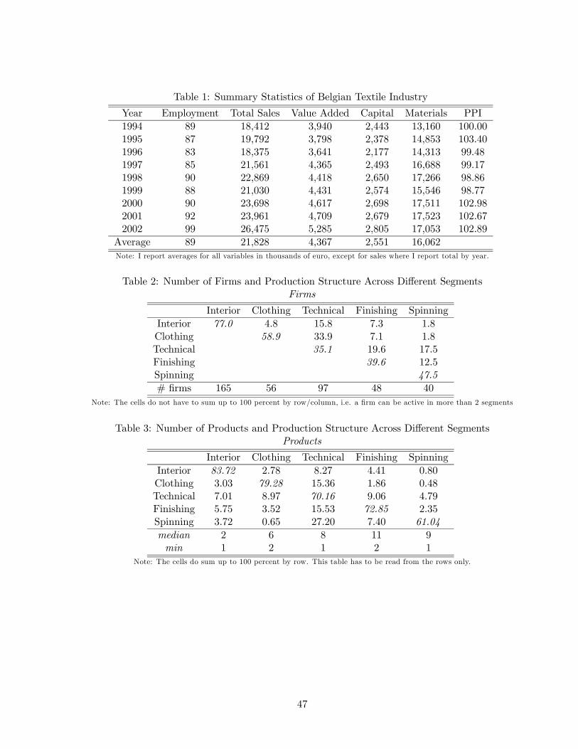
Table 1: Summary Statistics of Belgian Textile Industry

Year Employment Total Sales Value Added Capital Materials PPI1994 89 18,412 3,940 2,443 13,160 100.001995 87 19,792 3,798 2,378 14,853 103.401996 83 18,375 3,641 2,177 14,313 99.481997 85 21,561 4,365 2,493 16,688 99.171998 90 22,869 4,418 2,650 17,266 98.861999 88 21,030 4,431 2,574 15,546 98.772000 90 23,698 4,617 2,698 17,511 102.982001 92 23,961 4,709 2,679 17,523 102.672002 99 26,475 5,285 2,805 17,053 102.89

Average 89 21,828 4,367 2,551 16,062Note: I report averages for all variables in thousands of euro, except for sales where I report total by year.

Table 2: Number of Firms and Production Structure Across Different SegmentsFirms

Interior Clothing Technical Finishing SpinningInterior 77.0 4.8 15.8 7.3 1.8Clothing 58.9 33.9 7.1 1.8Technical 35.1 19.6 17.5Finishing 39.6 12.5Spinning 47.5# firms 165 56 97 48 40

Note: The cells do not have to sum up to 100 percent by row/column, i.e. a firm can be active in more than 2 segments

Table 3: Number of Products and Production Structure Across Different SegmentsProducts

Interior Clothing Technical Finishing SpinningInterior 83.72 2.78 8.27 4.41 0.80Clothing 3.03 79.28 15.36 1.86 0.48Technical 7.01 8.97 70.16 9.06 4.79Finishing 5.75 3.52 15.53 72.85 2.35Spinning 3.72 0.65 27.20 7.40 61.04median 2 6 8 11 9min 1 2 1 2 1

Note: The cells do sum up to 100 percent by row. This table has to be read from the rows only.

47

Table 4: The Estimated Coefficients of the Production Function

OLS KG Level KG Diff OP Augmented[1] [2] [3] [4] [5]β β α β α β β α

labor 0.2300 0.2319 0.2967 0.2451 0.3338 0.2113 0.2126 0.3075(0.0095) (0.0095) (0.0316) (0.0198) (0.0343) (0.0112) (0.0112) (0.0623)

materials 0.6298 0.6284 0.8041 0.5958 0.8115 0.6278 0.6265 0.9063(0.0074) (0.0074) (0.0770) (0.0131) (0.0519) (0.0085) (0.0084) (0.1746)

capital 0.0879 0.0868 0.1111 0.0188 0.0256 0.0931 0.1037 0.1500(0.0072) (0.0072) (0.0137) (0.0105) (0.0143) (0.0081) (0.0063) (0.0337)

output 0.2185 0.2658 0.3087(0.0749) (0.0462) (0.1335)

η -4.58 -3.76 -3.24markup 1.28 1.36 1.45Nr Obs 1,291 1,291 1,291 985 985

Note: β: estimated coefficients, α: production function coefficients.Bootstrapped standard errors are given in parentheses.

Table 5: Estimated Demand Parameters and Implied Firm Elasticities

A: Estimated Demand ParametersInterior Clothing Technical Finishing Spinning

βηs 0.1888* 0.2742* 0.2593* 0.3265* 0.1829*No product dummies (0.0742) (0.1029) (0.0907) (0.1042) (0.0774)

ηs (Sis = 1) -5.2966 -3.6470 -3.8565 -3.0628 -5.4675βηs 0.2315* 0.3140* 0.2952* 0.3178* 0.2437*

Product dummies (0.0541) (0.0756) (0.0648) (0.0756) (0.0585)(563 products) ηs (Sis = 1) -4.3196 -3.1847 -3.3875 -3.1466 -4.1034One Segment βηs 0.2641* 0.3550* 0.3575* 0.4563* 0.2556*(667 obs) ηs -3.7864 -2.8169 -2.7972 -2.1915 -3.9124

>1 Segments βηs 0.1673* 0.2267* 0.2253* 0.2241* 0.1455*(318 obs) ηs -5.9773 -4.4111 -4.4385 -4.4623 -6.8729

B: Implied Firm-Specific Demand Elasticities and markupsη η

η+1

mean -4.4486 1.3033s.d. 0.6915 0.0676

minimum -5.4059 1.2269maximum -3.1627 1.4624

Standard errors are given in parentheses and * denotes significance at 1 percent level.

48

Table 6: Number of Quota and Levels in Millions

Number of quota kg nr of piecesprotections # quota Level # quota Level

1994 1,046 466 3.10 580 8.581995 936 452 3.74 484 9.501996 824 411 3.70 413 7.951997 857 413 3.73 444 9.281998 636 329 4.21 307 9.011999 642 338 4.25 304 10.532000 636 333 4.60 303 9.772001 574 298 5.41 276 11.062002 486 259 5.33 227 12.37change -54% -44% 72% -60% 44%

Table 7: The Impact of Additional Demand Information: Quota Restriction

Specification (28)without Quota Information with Quota Information

Interior 0.2426* 0.1643*(0.0589) (0.0658)

Clothing 0.3475* 0.2381*Markups (0.0821) (0.0915)βηs Technical 0.3126* 0.2134*

(0.0710) (0.0796)Finishing 0.3364* 0.2219*

(0.0824) (0.0927)Spinning 0.2577* 0.1853*

(0.0637) (0.0690)βqr -0.0886*

quota restriction (0.0362)βl 0.2514* 0.2513*

(0.0124) (0.0123)βm 0.6785* 0.6808*

(0.0100) (0.0100)βk 0.0515* 0.0506*

(0.0101) (0.0122)returns to scale [1.30; 1.50] [1.16; 1.30]

Note: * indicates significant at 1%

49

Table 8: Impact Trade Liberalization on Productivity

Specification (# obs) Estimated coefficient Productivity Estimated usingaugmented model OP

I (1,291) qr -0.0637** -0.1068*(0.0366) (0.0296)

II (1,088) qr -0.0430* -0.0612*(0.0195) (0.0193)

III (1,088) 4qr -0.0699* -0.1254*(0.0312) (0.0327)

IV (1,088) 4qr -0.1172* -0.1605*(0.0374) (0.0393)

qrt−1 -0.0468* -0.0348*(0.0206) (0.0216)

V (765) 4qr -0.0455** -0.1347*(0.0272) (0.0299)

V I (890) qr -0.0584* -0.0664*(0.0229) (0.0226)

level 0.0019* -0.0000(0.0008) (0.0008)

Note: std errors in parentheses, * and ** denote significant at 5 or lower and 10 percent, resp.All regressions include quota-product classification dummies (23 categories), except for VI.

Table 9: Productivity Impact of a 10 percent Decrease in Protection Measure

Productivity Interior Clothing Technical Finishing Spinning OverallAugmented model 4.37 3.60 4.82 1.60 4.49 4.07

(1994-1997) 8.20 4.21 7.32 3.05 5.71 6.53(1998-2002) 2.28 3.23 3.32 0.72 3.75 2.59OP 8.06 6.45 8.63 2.86 8.04 7.28Note: The figures are elasticities evaluated at the mean by segment over the relevant period.

50

Table 10: Change in Average Quota Level (1994-2002)

Products measured inSupplying Country kilograms # pieces

Belarus 146 60China 83 38

Hong Kong 62 49India 56 127

Indonesia 90 78Malaysia 58 66

North Korea - 92Pakistan 129 144Peru 127 -

South Korea 61 69Taiwan 36 28Thailand 45 130Uzbekistan 556 -Vietnam -92 55Changes are expressed as a percentage.

51