Process monitoring using causal map and multivariate ...web.mit.edu/braatzgroup/54_Process_monitoring_using_causal_map_a… · Process monitoring using causal map and multivariate

Process monitoring using causal map and multivariate statistics:

fault detection and identification

Leo H. Chiang, Richard D. Braatz*

Large Scale Systems Research Laboratory, Department of Chemical Engineering, University of Illinois at Urbana-Champaign,

600 South Mathews Avenue, Box C-3 Urbana, IL 61801-3792, USA

Received 1 August 2001; received in revised form 13 April 2002; accepted 19 June 2002

Abstract

Data-driven techniques based on multivariate statistics (such as principal component analysis (PCA) and partial least squares

(PLS)) have been applied widely to chemical processes and their effectiveness for fault detection is well recognized. There is an

inherent limitation on the ability for purely data-driven techniques to identify and diagnose faults, especially when the abnormal

situations are associated with unknown faults or multiple faults. The modified distance (DI) and modified causal dependency

(CD) are proposed to incorporate the causal map with data-driven approach to improve the proficiency for identifying and

diagnosing faults. The DI is based on the Kullback–Leibner information distance (KLID), the mean of the measured variables,

and the range of the measured variable. The DI is used to measure the similarity of the measured variable between the current

operating conditions and the historical operating conditions. When the DI is larger than the predefined threshold, the variable is

identified as abnormal. The CD, derived based on the multivariate T2 statistic, is used to measure the causal dependency of two

variables. When CD is larger than the predefined threshold, the causal dependency of the two variables is broken. The proposed

method requires a causal map and historical data associated with the normal operating conditions. A causal map containing the

causal relationship between all of the measured variables can be derived based on knowledge from a plant engineer and the

sample covariance matrix from the normal data. The DI/CD algorithm outperformed the purely data-driven techniques such as

PCA for detecting and identifying known, unknown, and multiple faults using the data sets from the Tennessee Eastman process

(TEP).

D 2002 Elsevier Science B.V. All rights reserved.

Keywords: Fault detection; Fault identification; Process monitoring; Chemometrics methods; Causal map; Multivariate statistics

1. Introduction

Multivariate statistical methods such as principal

component analysis (PCA) and partial least square

(PLS) have been applied widely in chemical industries

for process monitoring [1–8]. An advantage of multi-

variate statistical methods is that they are completely

data-based—no sophisticated training is required for

an engineer to apply the techniques. Therefore, multi-

variate statistics are especially well-suited for large-

scale industrial processes. The main disadvantage of

the purely data-driven techniques is that there is an

inherent limitation on their ability to effectively iden-

tify and diagnose faults, especially when the abnormal

0169-7439/02/$ - see front matter D 2002 Elsevier Science B.V. All rights reserved.

doi:10.1016/S0169-7439(02)00140-5

* Corresponding author. Tel.: +1-217-333-5073; fax: +1-217-

333-5052.

E-mail address: [email protected] (R.D. Braatz).

www.elsevier.com/locate/chemometrics

Chemometrics and Intelligent Laboratory Systems 65 (2003) 159–178

Fig. 1. Example 1: (a) The normalized plot, (b) the KLID between the distribution and the flat distribution, (c) the mean, and (d) the range for

variable q under normal operating conditions.


variable q under normal operating conditions.

L.H. Chiang, R.D. Braatz / Chemometrics and Intelligent Laboratory Systems 65 (2003) 159–178160


variable q under faulty conditions.


variable q under faulty conditions.

L.H. Chiang, R.D. Braatz / Chemometrics and Intelligent Laboratory Systems 65 (2003) 159–178 161

situations are associated with unknown faults or

multiple faults. Knowledge-based approaches such

as the signed directed graph (SDG) [9–12], fault tree

analysis [13–15], and expert systems [16,17] have

been proposed to address these issues. These techni-

ques are based on qualitative models, which can be

obtained through causal modeling of the system,

expert knowledge, a detailed description of the sys-

tem, or fault-symptom examples.

The SDG, fault tree analysis, and expert systems

can improve fault diagnosis, but the main limitation to

applying these methods for large-scale systems is the

requirement of time-intensive collection of highly

detailed information for the system. To improve the

proficiency of data-driven techniques for fault identi-

fication and diagnosis, a less time-intensive method

which incorporates causal analysis and data-driven

techniques is proposed in this paper. Section 2

describes the entropy-based measures based on the

SELMON system, which provides some background

for understanding the proposed algorithm. This is

followed by a description of the proposed algorithm.

Section 3 evaluates the proposed method using data

sets from a chemical plant simulator. Section 4 sum-

marizes the conclusions.

2. Methods

2.1. Entropy-based measures

The SELective MONitoring (SELMON) system

was developed by Doyle et al. [18–20] in the artificial

intelligence research group at the Jet Propulsion

Laboratory. SELMON was designed to improve upon

the performance of traditional monitoring systems by

incorporating multiple measures to detect faults. SEL-

MON detects changes in the frequency distributions

Fig. 5. A diagram of the Tennessee Eastman process simulator.


of sensor readings over time; it also detects changes in

relationships among sensor readings. The two entropy-

based measures, which can be extended for fault diag-

nosis, are discussed here.

The entropy-based measures are the distance and

causal distance. Both measures are based on the

frequency distributions of the sensor measurements.

When a fault occurs, even if the observations or the

deviation measures are within their normal limits,

the frequency distribution of an observation variable

or the relationship between the frequency distribu-

tions of two variables can change significantly. The

distance and causal distance are designed for iden-

tifying these broken sensors and causal depend-

encies, respectively. The proficiency for detecting

and identifying faults can potentially increase by

integrating a causal map with the data-driven

approach.

The main advantage of the distance and causal

distance is that they are sensitive to faults associated

with changes in the distributions of the measured

variables. In situations where there are temporary

shifts of the data away from the mean, or changes in

variability of the measured variables around the mean,

the distance and causal distance can produce a lower

missed detection rate (type-II error) as compared to

multivariate statistics (such as PCA) [21].

However, a weakness of the distance and causal

distance is their strong dependence on the number of

bins and the size of each bin. The main disadvantage

is that collecting the data into different bins to define

the distribution loses resolution. Also, several distinct

distributions can result in the same measures. As such,

important information can be lost which often leads to

high false alarm rate (type-I error), especially for

large-scale systems [22].

2.2. Incorporating the causal map with the data-

driven approach

To take advantage of the entropy-based measures

and to avoid the disadvantage associated with using

bins, an algorithm based on the modified distance (DI)

and the causal dependence (CD) is proposed. The DI

is used to identify broken sensors, while the CD is

used to identify broken causal dependencies.

The DI is derived from the Kullback–Leibner

information distance (KLID), the mean of the meas-

ured variables, and the range of the measured varia-

bles. The continuous-time KLID [23] is defined as:

Iðp*; pÞ ¼Z

p*ðxÞlnp*ðxÞpðxÞ dx: ð1Þ

where p*(x) and p(x) are the distributions of the two

sensors under examination, and the random variable x

has been normalized by dividing the difference bet-

ween its maximum and minimum values so that 0VxV 1.

To illustrate the concept of the modified distance,

six examples will be shown. Examples 1 and 2 are

associated with the normal operating conditions, while

the rest are associated with faulty conditions. The data

from Example 1 are treated as the training set, while

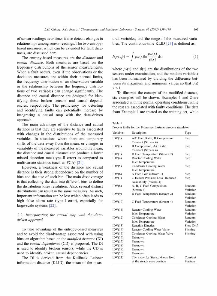
Table 1

Process faults for the Tennessee Eastman process simulator

Variable Description Type

IDV(1) A/C Feed Ratio, B Composition

Constant (Stream 4)

Step

IDV(2) B Composition, A/C Ratio

Constant (Stream 4)

Step

IDV(3) D Feed Temperature (Stream 2) Step

IDV(4) Reactor Cooling Water

Inlet Temperature

Step

IDV(5) Condenser Cooling Water

Inlet Temperature

Step

IDV(6) A Feed Loss (Stream 1) Step

IDV(7) C Header Pressure Loss–Reduced

Availability (Stream 4)

Step

IDV(8) A, B, C Feed Composition

(Stream 4)

Random

Variation

IDV(9) D Feed Temperature (Stream 2) Random

Variation

IDV(10) C Feed Temperature (Stream 4) Random

Variation

IDV(11) Reactor Cooling Water

Inlet Temperature

Random

Variation

IDV(12) Condenser Cooling Water

Inlet Temperature

Random

Variation

IDV(13) Reaction Kinetics Slow Drift

IDV(14) Reactor Cooling Water Valve Sticking

IDV(15) Condenser Cooling Water Valve Sticking

IDV(16) Unknown

IDV(17) Unknown

IDV(18) Unknown

IDV(19) Unknown

IDV(20) Unknown

IDV(21) The valve for Stream 4 was fixed

at the steady state position

Constant

Position


the data from the rest of the examples are treated as

the testing set.

In Example 1, 200 observations for measured

variable q are simulated under the normal distribution

with mean zero and variance one. The variable has

been normalized by its absolute minimum and max-

imum values (see Fig. 1a).

With the window size is specified as b = 20, the

historical distribution ph,tq is calculated for t= n� b + 1

to n, where n= 200. The KLID between the historical

distribution for q and a flat distribution (often called a

uniform distribution, i.e., p(x) = 1)

fqh;t ¼ Iðpqh;t; 1Þ; ð2Þ

is calculated based on numerical integration. If ph,tq is a

flat distribution, then f h,tq is equal to zero. Fig. 1b shows

that f h,tq ranges from 1.3 to 2.1, indicating that the

distribution is clearly different from a flat distribution.

For recent observations simulated under the same

normal operating conditions as in Example 1, fr,tq is

expected to fall inside the same range as f h,tq . To verify

that, another 200 observations for measured variable q

are simulated in Example 2 under the same condition.

The testing data for variable q has been normalized by

the absolute minimum and maximum values used in

Example 1 (see Fig. 2).

Using the same window size b = 20, the recent

distribution pr,tq is calculated for t = n� b + 1 to n in

Example 2. The KLID between pr,tq and a flat distri-

bution is

fqr;t ¼ Iðpqr;t; 1Þ; ð3Þand the result is shown in Fig. 2b. The range for fr,t

q is

similar to the range for fh,tq, indicating that the dis-

tributions for q may be similar in both examples.

In Example 3, a fault condition is introduced at

t = 30, in which the variation of variable q decreases

(see Fig. 3a). Fig. 3b shows that fr,tq increases to 4.8 at

t = 55, indicating that the distribution has deviated

from the normal conditions in Example 1. The small

variations of q for t>55 is reflected in fr,tq, which also

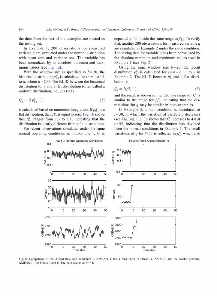
Fig. 6. Comparison of the A feed flow rate in Stream 1, XMEAS(1), the A feed valve in Stream 1, XMV(3), and the reactor pressure,

XMEAS(7), for Faults 0 and 6. The fault occurs at t = 8 h.


shows smaller variations for t>55. The detection delay

is about 17 in this example. In general, a large

window size b will result in a large detection delay,

while a small window size b will result in a less

sensitive fault detection statistic.

In Example 4, the variables drift for tz 30 (see Fig.

4a). The ranges for fr,tq in both examples are very

similar to the range of f h,tq , suggesting that fr,t

q is not

sensitive in detecting shifts in mean. A statistic based

solely on fr,tq is not able to detect the changes effec-

tively in Examples 3 and 4.

Examples 1 and 2 illustrate that similar KLIDs are

obtained when the variable is associated with similar

operating conditions. Examples 3 to 4 illustrate that fr,tq

is sensitive for detecting changes in the variance of a

variable, but insensitive for detecting drift in a vari-

able. KLID depends only on the distribution pr,tq and

the magnitude of the variable is not taken into account

directly. This motivates the incorporation of additional

measures for detecting faults.

In most cases, the effect of the faulty conditions on

the variables is reflected in the mean of the variables

or the range of the variables.

For recent observations in a window with size b,

the mean of the variable q at current time t = T is

mqr;t ¼

1

b

XTt¼T�bþ1

qt; ð4Þ

where qt is the observation for q at time t. Alterna-

tively, the shift in mean can be detected using cumu-

lative sum chart (CUSUM) or an exponentially

weighted moving average chart (EWMA) [24–26].

The range of the variable q is

sqr;t ¼ max

T�bþ1VtVTqt � min

T�bþ1VtVTqt: ð5Þ

In Example 3, sr,tq drops to nearly zero for t>50 (see

Fig. 3d), indicating that sr,tq will be able to detect the

change in Example 3. In Example 4, mr,tq indicates that

the variable is drifting (see Fig. 4c). Incorporating fr,tq,

mr,tq , and sr,t

q can provide a more sensitive fault detection

statistic than the SELMON statistics in Section 2.1.

A normalization is used for fr,tq, mr,t

q , and sr,tq to

compare between a recent distribution and a historical

distribution. With f hqdefined as the I( fh,t

q,1) with the

window size b, the adjusted fr,tq is defined by

fqr;t ¼ Af qr;t � f

q

hA; ð6Þ

with this step, the positive and negative shifts from the

historical distribution can be detected. The normalized

KLID is defined by

Fqr;t ¼

fqr;t

meanðf qh;tÞ þ nrstdðf qh;tÞ; ð7Þ

where std denotes standard deviation, f h,tq =Af h,t

q � f hqA,

and nr is a constant used to specify the type-I error,

which can be determined based on the historical data.

For a large-scale system, a higher nr is desired in order

to achieve a lower overall false alarm rate. Alterna-

tively, fr,tq can be divided by the maximum value of f h,t

q

to obtain the normalization.

Similarly, the adjusted mr,tq is defined by

mqr;t ¼ Amq

r;t � mq

hA; ð8Þ

where mhqis the mean of variable q in the entire

training set, which is equal to 0.5. The adjusted sr,tq is

defined by

sqr;t ¼ Asqr;t � s

q

hA; ð9Þ

where shqis the range of the variable q in the entire

training set.

Table 2

The false alarm rate (type-I error) for the testing set of Fault 0 and

the missed detection rates (type-II error) for the testing sets for

Faults 1–21 using the modified distance (models derived based on

training set for Fault 0, which contains 480 observations)

Fault DI CD DI/CD

0 0.026 0.0200 0.0462

1 0.009 0.0012 0.003

2 0.020 0.013 0.013

3 0.890 0.928 0.866

4 0 0 0

5 0.006 0 0

6 0.005 0 0

7 0 0 0

8 0.031 0.011 0.015

9 0.903 0.934 0.885

10 0.174 0.153 0.080

11 0.008 0.175 0.006

12 0.004 0.003 0.003

13 0.051 0.051 0.050

14 0.001 0 0

15 0.774 0.824 0.751

16 0.254 0.088 0.051

17 0.029 0.043 0.026

18 0.108 0.094 0.095

19 0.068 0.441 0.036

20 0.106 0.130 0.080

21 0.056 0.476 0.056

Overall 0.166 0.208 0.144


The normalized mr,tq and sr,t

q are defined by

Mqr;t ¼

mqr;t

meanðmqh;tÞ þ nrstdðmq

h;tÞ; ð10Þ

and

Sqr;t ¼

sqr;t

meanðsqh;tÞ þ nrstdðsqh;tÞ; ð11Þ

respectively.

The modified DI is defined by

DIqt ¼ A F

qr;t

Cqr;t

Fqr;tC

qr;t

266664

377775

A; ð12Þ

where Cr,tq takes the larger value between M r,t

q and Sr,tq .

Note that either Sr,tq or M r,t

q contributes to the mo-

dified DI. For most observable faults (see Figs.

3c,d and 4c,d), faulty conditions do not usually

effect both sr,tq and mr,t

q , so including both terms in

the modified DI would result in a less sensitive

fault detection statistic.

To use DI tq for fault detection, a pre-specified

threshold based on the training data associated with

the normal operating conditions is required. The

thresholds for Fr,tq , M r,t

q , and Sr,tq are one. Therefore,

the threshold for DItq is specified as

ffiffiffi3

p.

Recall that Example 2 is associated with the testing

set for the normal operating conditions. It is expected

that the distance measure DItq should be less than the

threshold for nearly all observations. Calculations

show that the false alarm rate for DItq is small (1/180),

indicating that the threshold is well-defined. The nor-

malized modified distance is able to detect the faults

promptly for Examples 3 and 4.

The modified distance measure is used to detect a

change in the frequency distribution for each measure

variable. To quantify the similarity between each

causal relationship associated with the causal map

under current operating conditions and historical nor-

mal operating conditions, the causal dependence (CD)

is used.

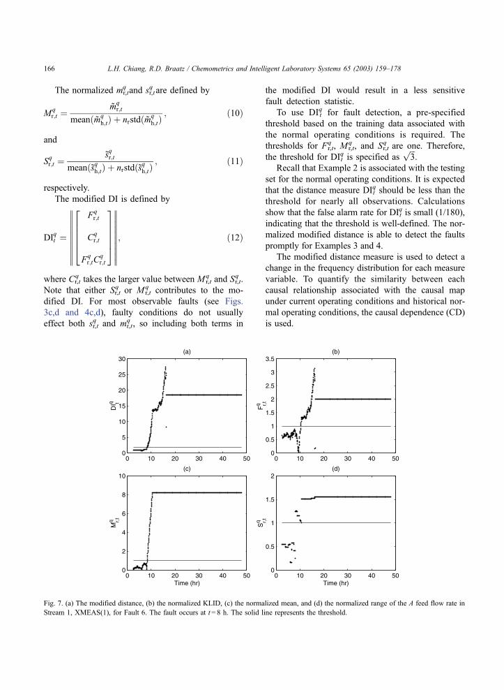
Fig. 7. (a) The modified distance, (b) the normalized KLID, (c) the normalized mean, and (d) the normalized range of the A feed flow rate in

Stream 1, XMEAS(1), for Fault 6. The fault occurs at t = 8 h. The solid line represents the threshold.


For causal dependency, define c as the cause

variable and e as the effect variable. The CD is based

on the multivariate T2 statistic, which is defined by

CDc;e ¼ T 2c;e ¼ ðy � yÞTS�1

c;e ðy � yÞ; ð13Þ

where y=[c e]T, y is the mean of y, and Sc,e is the

sample covariance for variables c and e. Full rank is

taken for the T2 statistic. The threshold for Tc,e2 is

CDa ¼ T2a ¼ 2ðn� 1Þðnþ 1Þ

nðn� 2Þ Fað2; n� 2Þ; ð14Þ

where n is the number of observations in the training

sets and a is the level of significance [27]. Assuming

that c and e follow a normal distribution, a false alarm

rate a is expected for the T2 statistic. Let the total

number of causal dependencies in the process be nCD,

then the overall type-I error is

atotal ¼ 1� ð1� aÞnCD : ð15Þ

For small nCD, atotal is comparable with a; for largenCD, atotal is larger than a. For fault detection, the

desired type-I error atotal is first specified, then the

threshold T2a for each causal dependency is calculated

using Eqs. (14) and (15).

The training data associated with the normal

operating conditions (denoted as Fault 0) is required

for fault detection. The data in the training set,

consisting of m observation variables and n observa-

tions for each variable, are stacked into a matrix

XaRn� m, given by

X ¼

x11 x12 . . . x1m

x21 x22 . . . x2m

] ] . . . ]

xn1 xn2 . . . xnm

2666666664

3777777775: ð16Þ

With the window size specified for each variable, the

historical distribution ph,t,0q , the mean mh,t,0

q , and the

range sh,t,0q associated with each variable are com-

Fig. 8. (a) The modified distance, (b) the normalized KLID, (c) the normalized mean, and (d) the normalized range of the A feed valve in Stream

1, XMV(3), for Fault 6. The fault occurs at t = 8 h. The solid line represents the threshold.


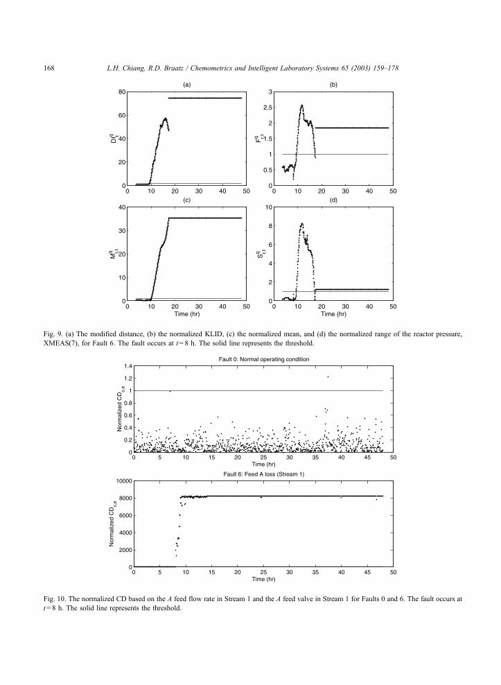
Fig. 9. (a) The modified distance, (b) the normalized KLID, (c) the normalized mean, and (d) the normalized range of the reactor pressure,

XMEAS(7), for Fault 6. The fault occurs at t= 8 h. The solid line represents the threshold.

Fig. 10. The normalized CD based on the A feed flow rate in Stream 1 and the A feed valve in Stream 1 for Faults 0 and 6. The fault occurs at

t = 8 h. The solid line represents the threshold.


puted. In addition, ph,0q, mh,0

q, and sh,0

qare computed

using n observations for each variable. A fault

associated with a sensor or sensor changing its

character is detected for the variable q if

DIqt > DIa: ð17Þ

To detect broken causal dependencies among var-

iables, a causal map containing the causal relationship

between all of the measured variables is required. The

causal map can be derived based on knowledge from a

plant engineer. The sample covariance matrix from the

normal data can be used to verify the accuracy of the

causal map. Two variables are related when the

correlation is high. Based on the training data for

Fault 0, the sample covariance Sc,e and the mean of the

variable y=[c e]T are computed for each causal depend-

ency. The threshold is calculated using Eqs. (14) and

(15). The causal relationship between two variables is

broken when

T2c;e > T2

a ; ð18Þ

and Eq. (17) is satisfied for variables c and e. In other

words, the causal relationship remains normal for c and

e as long as Eq. (17) is satisfied for either variables.

When a fault is detected, the variables c and e

which satisfy Eqs. (17) and (18) represent the fault

propagation path (denoted as FPt). Such fault prop-

agation information plays an important role in isolat-

ing and determining the root cause.

Once a fault has been detected, the next step is to

determine the cause of the out-of-control status. The

task of diagnosing the fault can be rather challenging

when the number of process variables is large, and the

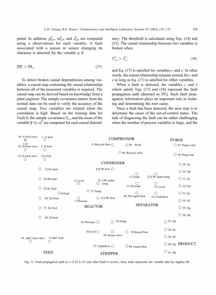
Fig. 11. Fault propagation path at t = 8.25 h (15 min after Fault 6 occurs). Grey node represents the variable that has highest DI.


process is highly integrated. Also, many of the meas-

ured variables may deviate from their set-points for

only a short time period when a fault occurs, due to

control loops bringing the variables back to their set-

points (even though the fault is persisting in the

system). This type of systems behavior can disguise

the fault, making it difficult for an automated fault

diagnosis algorithm to correctly isolate the correct

fault acting on the system.

The goal of fault identification is to identify the

variables which are most related with the fault

origin, thereby focusing the plant operators and

engineers on the subsystem(s) most likely where

the fault occurred. This assistance provided by the

fault identification scheme in locating the fault can

effectively incorporate the operators and engineers in

the process monitoring scheme and significantly

reduce the time to recover in-control operations.

The magnitudes of the DI and CD represent the

degree to which the variables have deviated from

their distributions in the normal operating conditions.

Root causes are often highly correlated with the

variables which have the highest DI and the causal

dependency which has the highest CD. Proper and

immediate actions to those variables can prevent the

effect of the fault from propagating to other varia-

bles.

3. Application

3.1. Tennessee Eastman process

The process simulator for the Tennessee Eastman

process (TEP) was created by the Eastman Chemical

to provide a realistic industrial process for evaluating

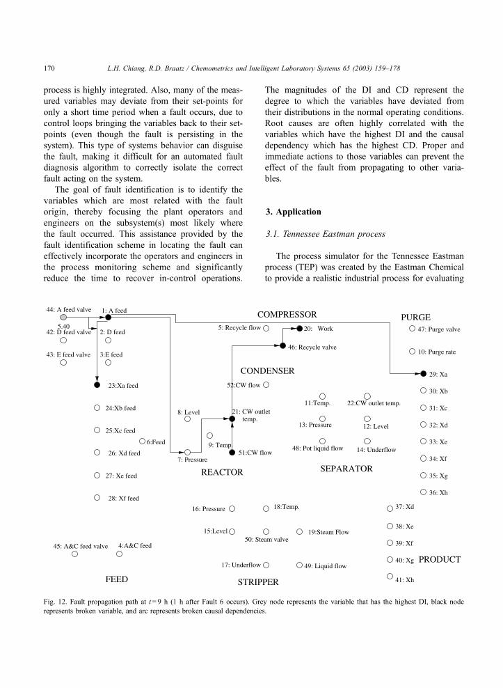
Fig. 12. Fault propagation path at t = 9 h (1 h after Fault 6 occurs). Grey node represents the variable that has the highest DI, black node

represents broken variable, and arc represents broken causal dependencies.


process control and monitoring methods [28]. The TE

process simulator has been widely used by the process

monitoring community as a source of data for com-

paring various approaches [1–3,7,8,29–40].

The chemical plant simulator is based on an indus-

trial process where the components, kinetics, and

operating conditions were modified for proprietary

reasons (see Fig. 5). The gaseous reactants A, C, D,

and E and the inert B are fed to the reactor where the

liquid products G and H are formed. The reactions in

the reactor are irreversible, exothermic, and approx-

imately first-order with respect to the reactant concen-

trations. The reactor product stream is cooled through

a condenser and then fed to a vapor–liquid separator.

The vapor exiting the separator is recycled to the

reactor feed through the compressor. A portion of the

recycle stream is purged to keep the inert and byprod-

ucts from accumulating in the process. The condensed

components from the separator (Stream 10) are

pumped to the stripper. Stream 4 is used to strip the

remaining reactants in Stream 10, and is combined

with the recycle stream. The products G and H exiting

the base of the stripper are sent to a downstream

process which is not included in this process. The

simulation code allows 21 preprogrammed major

process faults, as shown in Table 1. The plant-wide

control structure recommended in Lyman and Geor-

gakis [41] was implemented to generate the closed

loop simulated process data for each fault.

One simulation run (Fault 0) was generated with no

faults for the training set. No training sets were

generated for Faults 1–21. The simulation time for

each run was 25 h.

The data in the testing set consisted of 22 different

simulation runs, where the random seed was changed

between each run. The first 16 simulation runs directly

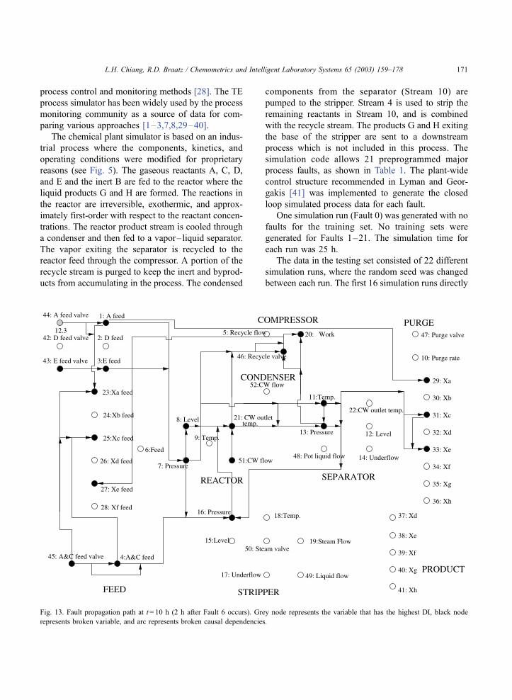
Fig. 13. Fault propagation path at t= 10 h (2 h after Fault 6 occurs). Grey node represents the variable that has the highest DI, black node

represents broken variable, and arc represents broken causal dependencies.


correspond to the runs in the training set (Faults 0–15).

One simulation run (Fault 21) was generated by fixing

the position of the valve for Stream 4 at the steady state

position. Five more simulation runs (Faults 16–20)

were simulated under unknown conditions, specified

by the original TEP simulator. The simulation time for

each run was 48 h. The simulation started with no

faults, and the faults were introduced 8 simulation h

into the run. The total number of observations gener-

ated for each run was n = 960.

The causal map can be constructed in a straightfor-

ward manner using a fundamental mathematical

model of the process. Because a fundamental model

of the TEP is assumed to be unavailable, the causal

model used in this work was constructed based on the

knowledge of the process and the correlation coeffi-

cients associated with the data from normal operating

conditions.

3.2. Case studies

Selective case studies are discussed here to illus-

trate the proficiency of the proposed algorithm.

Detailed discussion of the results are available [22].

3.2.1. Fault 6

For Fault 6, there is a feed loss of A in Stream 1 at

t = 8 h (see XMEAS(1) in Fig. 6), which causes the

control loop on Stream 1 to fully open the A feed

valve (see XMV(3) in Fig. 6). Because there is no

reactant A in the feed, the reaction will eventually

stop. This causes the gaseous reactants D and E build

up in the reactor, and hence the reactor pressure

increases (see XMEAS(7) in Fig. 6). The reactor

pressure continues to increase until it reaches the

safety limit of 2950 kPa, at this point the valve for

Control Loop 6 is fully open. Clearly, it is very

Fig. 14. Fault propagation path at t= 13 h (5 h after unknown Fault 18 occurs). Grey node represents the variable that has the highest DI, black

node represents broken variable, and arc represents broken causal dependencies.


important to detect this fault promptly before the fault

upsets the whole process.

The DI and CD detect Fault 6 effectively (see Table

2). Fig. 7 shows that the modified distance increases

up to 28 for the A feed flow rate, which is 16 times the

threshold. The A feed flow rate decreases from about

0.25 to 0 at t = 8 h (see Fig. 6) and it remains steady at

0 for t>8 h. Because the mean and range of the A feed

flow rate change significantly, the normalized mean

and the normalized range both promptly detect the

fault. The flat distribution for t>8 h is also detected by

the KLID.

Similarly to the A feed flow rate in Stream 1,

extreme changes associated with the mean, range,

and distribution are found in the A feed valve in

Stream 1 and the reactor pressure (see Figs. 8 and

9). As a result, the KLID, the normalized mean, and

the normalized range are able to detect Fault 6

promptly (see Fig. 7).

The CDc,e, associated with the A feed valve and the

A feed flow rate is shown in Fig. 10. The CD increases

up to 8000 times the threshold, indicating extreme

changes in the means for these two variables.

Fig. 11 shows the fault propagation path 15 min

(five sampling intervals) after the fault occurs, the

normalized modified distance for the A feed valve in

Stream 1 is 1.61. The normalized modified distance is

less than one for the rest of the variables. The feed

0 10 20 30 40 500

10

20

30

40

XM

EA

S(1

1)

DIqt

0 10 20 30 40 5074

76

78

80

82

84

86X

ME

AS

(11)

Measured Variables

0 10 20 30 40 500

20

40

60

80

100

120

Time (hr)

XM

EA

S(2

2)

0 10 20 30 40 5060

65

70

75

80

Time (hr)

XM

EA

S(2

2)

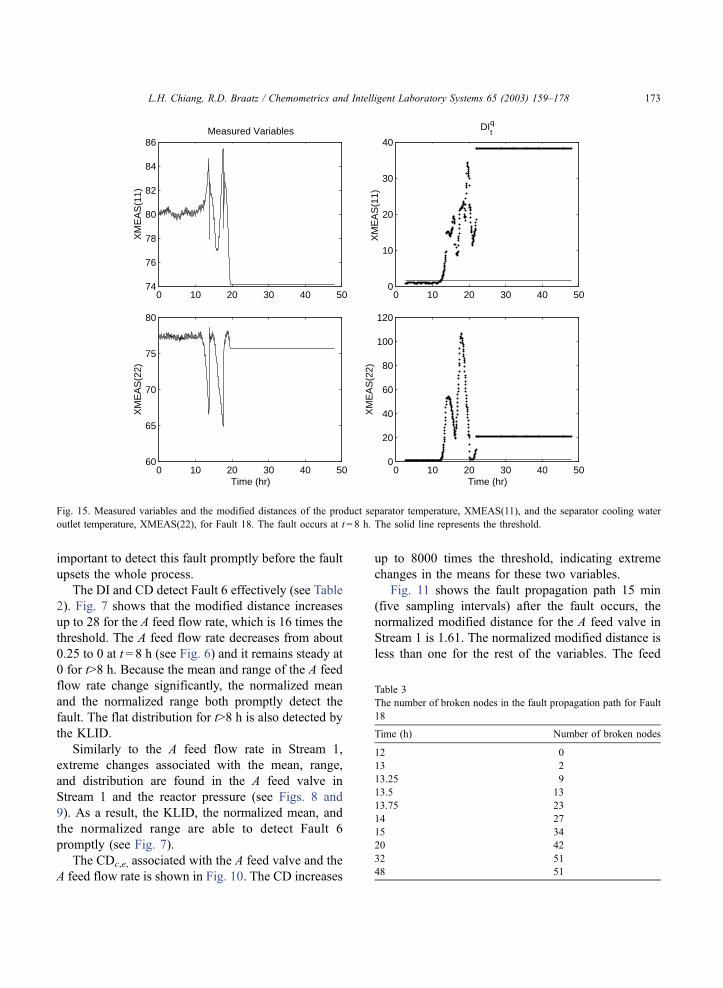
Fig. 15. Measured variables and the modified distances of the product separator temperature, XMEAS(11), and the separator cooling water

outlet temperature, XMEAS(22), for Fault 18. The fault occurs at t = 8 h. The solid line represents the threshold.

Table 3

The number of broken nodes in the fault propagation path for Fault

18

Time (h) Number of broken nodes

12 0

13 2

13.25 9

13.5 13

13.75 23

14 27

15 34

20 42

32 51

48 51


valve for A is promptly identified as the root cause for

Fault 6.

Fig. 12 shows the fault propagation path 1 h after

the fault occurs. The effects of Fault 6 propagate to

other variables. The normalized modified distance for

the A feed valve has the highest magnitude, which is

5.40. Two hours after Fault 6 occurs, the normalized

modified distance for 21 out of 52 variables are larger

than one (see Fig. 13), indicating that the fault has

deeply affected most variables. The normalized modi-

fied distance for the A feed valve further increases to

12.3, which continues to represent the highest score

among all 52 variables. The number of broken vari-

ables in the fault propagation path increases to 38 and

46, respectively, after 5 and 20 h have passed. This

example is effective in illustrating the importance in

promptly detecting and identifying the fault using the

modified distance before the whole process is being

upset. This also shows that the modified distance can

promptly and effectively identify the fault, and that a

visualization of the fault propagation path constructed

from these statistics can be valuable for operators to

understand how the fault is affecting the process.

3.2.2. Fault 18

The author of the Tennessee Eastman plant simu-

lator purposely does not reveal the root causes for the

unknown Faults 16 to 20. The fault propagation paths

can provide useful information to reveal the root causes

in these cases. For 5 h after Fault 18 occurs (t = 8 to 13

h), all 52 variables behave normally and no broken

nodes are recorded in the fault propagation path. At

t = 13 h, the nodes for the separator temperature,

XMEAS(11), and the separator cooling water outlet

temperature, XMEAS(22), are broken (see Fig. 14).

The arcs between the variables are also broken. Fig. 15

confirms that the separator behaves abnormally. The

effect of Fault 18 is severe and the control loops are not

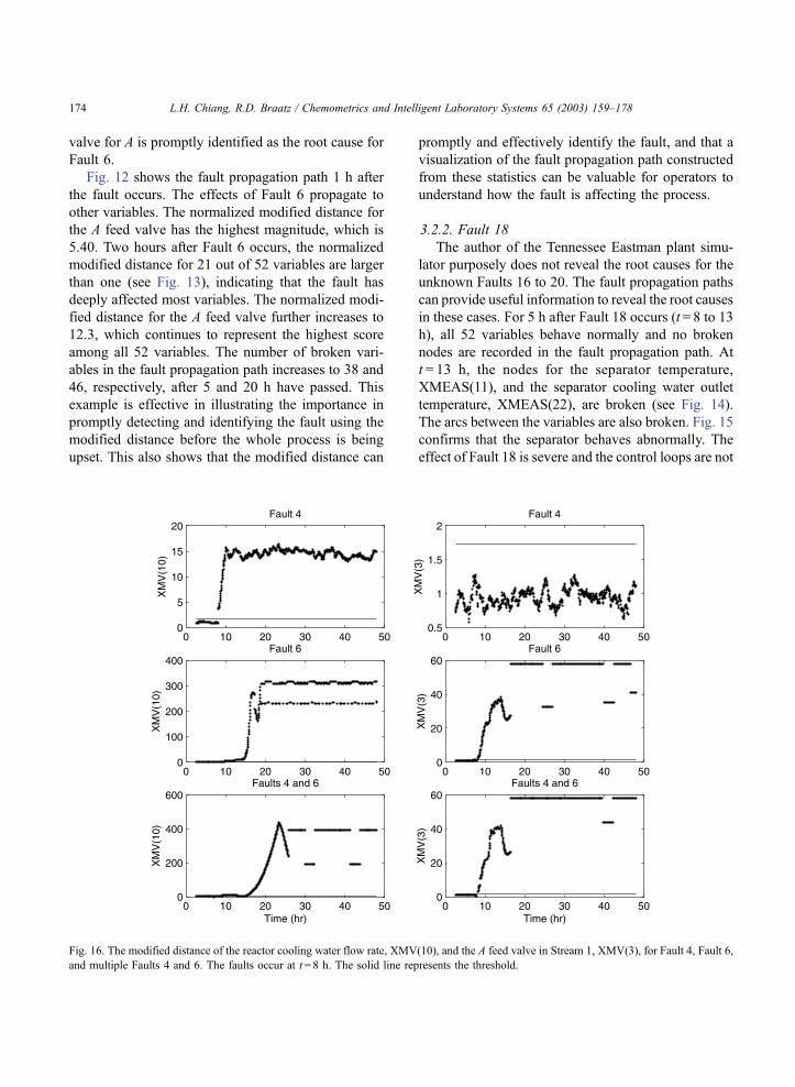
Fig. 16. The modified distance of the reactor cooling water flow rate, XMV(10), and the A feed valve in Stream 1, XMV(3), for Fault 4, Fault 6,

and multiple Faults 4 and 6. The faults occur at t = 8 h. The solid line represents the threshold.


able to compensate for the fault. At t = 14 h, 27 broken

nodes are recorded in the fault propagation path (see

Table 3); at t= 32 h, 51 out of 52 nodes are broken. The

modified distance is able to identify and isolate Fault 18

before the whole process is upset.

3.2.3. Multiple Faults 4 and 6

Multiple Faults 4 and 6 are masked multiple faults,

in which the variables affected by one fault are a subset

of the variables affected by another fault. The previous

discussions show that Fault 6 involves unsteady oper-

ations, causing most variables to deviate significantly

from their normal behaviors. Although Fault 4 has a

clear effect on the reactor cooling water flow rate, the

effect of Fault 4 is masked whenmultiple Faults 4 and 6

occur. This is confirmed by the modified distances for

the reactor cooling water flow rate and the A feed valve

in Stream 1 (see Fig. 16).

Three minutes after multiple Faults 4 and 6

occur two disjointed fault propagation paths appear

(see Fig. 17). This is an indication that multiple

faults occurred. The fault propagation path contain-

ing the reactor temperature and the reactor cooling

water outlet temperature represents the symptoms

for Fault 4, while the fault propagation path con-

taining the A feed valve represents the symptom for

Fault 6.

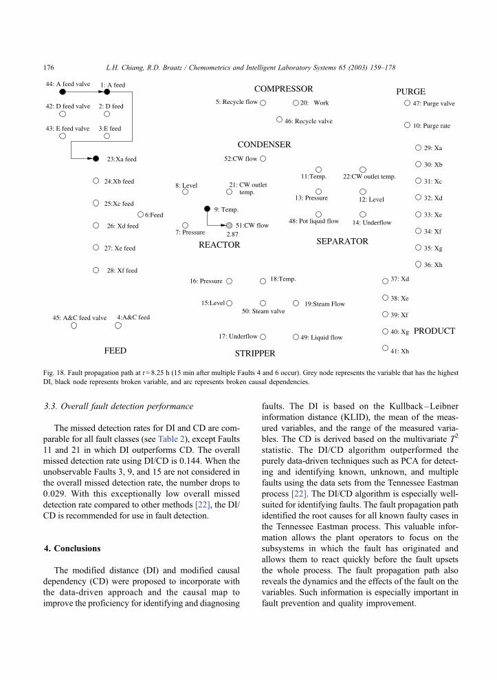
Forty five minutes after the faults occur, the num-

ber of variables in one fault propagation increases

to three, while the number of variables in the other

fault propagation remain the same (see Fig. 18).

This shows that Fault 6 has propagated to more

variables. Seventy five minutes after the faults occur,

the total number of variables in the fault propagation

path increases to 9, in which Fault 4 is masked by

Fault 6.

Fig. 17. Fault propagation path at t = 8.05 h (3 min after multiple Faults 4 and 6 occur). Grey node represents the variable that has the highest DI,

black node represents broken variable, and arc represents broken causal dependencies.


3.3. Overall fault detection performance

The missed detection rates for DI and CD are com-

parable for all fault classes (see Table 2), except Faults

11 and 21 in which DI outperforms CD. The overall

missed detection rate using DI/CD is 0.144. When the

unobservable Faults 3, 9, and 15 are not considered in

the overall missed detection rate, the number drops to

0.029. With this exceptionally low overall missed

detection rate compared to other methods [22], the DI/

CD is recommended for use in fault detection.

4. Conclusions

The modified distance (DI) and modified causal

dependency (CD) were proposed to incorporate with

the data-driven approach and the causal map to

improve the proficiency for identifying and diagnosing

faults. The DI is based on the Kullback–Leibner

information distance (KLID), the mean of the meas-

ured variables, and the range of the measured varia-

bles. The CD is derived based on the multivariate T2

statistic. The DI/CD algorithm outperformed the

purely data-driven techniques such as PCA for detect-

ing and identifying known, unknown, and multiple

faults using the data sets from the Tennessee Eastman

process [22]. The DI/CD algorithm is especially well-

suited for identifying faults. The fault propagation path

identified the root causes for all known faulty cases in

the Tennessee Eastman process. This valuable infor-

mation allows the plant operators to focus on the

subsystems in which the fault has originated and

allows them to react quickly before the fault upsets

the whole process. The fault propagation path also

reveals the dynamics and the effects of the fault on the

variables. Such information is especially important in

fault prevention and quality improvement.

Fig. 18. Fault propagation path at t = 8.25 h (15 min after multiple Faults 4 and 6 occur). Grey node represents the variable that has the highest

DI, black node represents broken variable, and arc represents broken causal dependencies.


Acknowledgements

This work was supported by International Paper

and the National Center for Supercomputing Appli-

cations. The authors would like to thank Randy Pell at

the Dow Chemical Company for his comments, which

significantly improved the paper.

References

[1] L.H. Chiang, E.L. Russell, R.D. Braatz, Fault Detection and

Diagnosis in Industrial Systems, Springer Verlag, London,

2001.

[2] E.L. Russell, L.H. Chiang, R.D. Braatz, Data-driven Techni-

ques for Fault Detection and Diagnosis in Chemical Processes,

Springer Verlag, London, 2000.

[3] E.L. Russell, L.H. Chiang, R.D. Braatz, Fault detection in

industrial processes using canonical variate analysis and dy-

namic principal component analysis, Chemometrics and Intel-

ligent Laboratory Systems 51 (2000) 81–93.

[4] R. Dunia, S.J. Qin, Joint diagnosis of process and sensor faults

using principal component analysis, Control Engineering

Practice 6 (1998) 457–469.

[5] T. Kourti, J.F. MacGregor, Multivariate SPC methods for

process and product monitoring, Journal of Quality Technol-

ogy 28 (1996) 409–428.

[6] B.R. Bakshi, Multiscale PCA with application to multivariate

statistical process monitoring, AIChE Journal 44 (1998)

1596–1610.

[7] A.C. Raich, A. Cinar, Statistical process monitoring and dis-

turbance diagnosis in multivariable continuous processes,

AIChE Journal 42 (1996) 995–1009.

[8] W. Ku, R.H. Storer, C. Georgakis, Disturbance detection

and isolation by dynamic principal component analysis, Che-

mometrics and Intelligent Laboratory Systems 30 (1995)

179–196.

[9] M. Iri, K. Aoki, E. O’Shima, H. Matsuyama, An algorithm for

diagnosis of system failures in the chemical process, Com-

puters & Chemical Engineering 3 (1979) 489–493.

[10] J. Shiozaki, H. Matsuyama, E. O’Shima, M. Iri, An improved

algorithm for diagnosis of system failures in the chemical proc-

ess, Computers & Chemical Engineering 9 (1985) 285–293.

[11] Y. Tsuge, J. Shiozaki, H. Matsuyama, E. O’Shima, Fault diag-

nosis algorithms based on the signed directed graph and its

modifications, Industrial and Chemical Engineering Symposi-

um Series 92 (1985) 133–144.

[12] I.P. Gal, K.M. Hangos, SDG model-based structures for fault

detection, Proc. of the IFAC On-line Fault Detection and

Supervision in the Chemical Process Industries, Piscataway,

NJ, IEEE Press, 1998, pp. 243–248.

[13] D.J. Allen, Digraphs and fault trees, Industrial & Engineering

Chemistry Fundamentals 23 (1984) 175–180.

[14] S.A. Lapp, G.J. Power, Computer-aided synthesis of fault tree,

IEEE Transactions on Reliability 28 (1977) 2–13.

[15] W.G. Schneeweiss, Fault tree analysis in case of multiple

faults, especially covered and uncovered ones, Microelec-

tronics and Reliability 38 (1998) 659–663.

[16] T.F. Petti, J. Klein, P.S. Dhurjati, Diagnostic model processor.

Using deep knowledge for process fault diagnosis, AIChE

Journal 36 (1990) 565–575.

[17] J. Zhao, B. Chen, J. Shen, A hybrid ANN-ES system for

dynamic fault diagnosis of hydrocracking process, Computers

& Chemical Engineering 21 (1997) S929–S933.

[18] R.J. Doyle, Determining the loci of anomalies using minimal

causal models, International Joint Conference on Artificial

Intelligence, American Association for Artificial Intelligence,

Montreal, Canada, 1995 (August), pp. 1a–7a.

[19] R.J. Doyle, L. Charest, N. Rouquette, J. Wyatt, C. Robertson,

Causal modeling and event-driven simulation for monitoring

of continuous systems, Computers in Aerospace 9 (1993)

395–405.

[20] R.J. Doyle, S.A. Chien, U.M. Fayyad, E.J. Wyatt, Focused

real-time systems monitoring based on multiple anomaly mod-

els, 7th Int. Workshop on Qualitative Reasoning, Eastsound,

Washington, May, 1993.

[21] E.L. Russell. Process Monitoring of Large Scale Systems.

PhD thesis, University of Illinois, Urbana, IL, 1998.

[22] L.H. Chiang. Fault Detection and Diagnosis for Large-Scale

Systems. PhD thesis, University of Illinois, Urbana, IL, 2001.

[23] L. Ljung, System Identification: Theory for the User, Prentice-

Hall, Englewood Cliffs, NJ, 1987.

[24] P. Fasolo, D.E. Seborg, SQC approach to monitoring and

fault detection in HVAC control systems, Proc. of the Amer-

ican Control Conf., Piscataway, NJ, vol. 3, IEEE Press, 1994,

pp. 3055–3059.

[25] D.C. Montgomery, Introduction to Statistical Quality Control,

Wiley, New York, 1985.

[26] B.A. Ogunnaike, W.H. Ray, Process Dynamics, Modeling,

and Control, Oxford Univ. Press, New York, 1994.

[27] J.F. MacGregor, T. Kourti, Statistical process control of multi-

variate processes, Control Engineering Practice 3 (1995)

403–414.

[28] J.J. Downs, E.F. Vogel, A plant-wide industrial-process con-

trol problem, Computers & Chemical Engineering 17 (1993)

245–255.

[29] L.H. Chiang, E.L. Russell, R.D. Braatz, Fault diagnosis in

chemical processes using Fisher discriminant analysis, dis-

criminant partial least squares, and principal component anal-

ysis, Chemometrics and Intelligent Laboratory Systems 50

(2000) 243–252.

[30] A.C. Raich, A. Cinar, Multivariate statistical methods for

monitoring continuous processes: assessment of discrimina-

tory power disturbance models and diagnosis of multiple dis-

turbances, Chemometrics and Intelligent Laboratory Systems

30 (1995) 37–48.

[31] A.C. Raich, A. Cinar, Process disturbance diagnosis by stat-

istical distance and angle measures, Proc. of the 13th IFAC

World Congress, Piscataway, NJ, IEEE Press, 1996, pp. 283–

288.

[32] H.B. Aradhye, B.R. Bakshi, R. Strauss, Process monitoring by

PCA, dynamic PCA, and multiscale PCA—Theoretical anal-


ysis and disturbance detection in the Tennessee Eastman proc-

ess. AIChE Annual Meeting, 1999, Paper 224g.

[33] G. Chen, T.J. McAvoy, Predictive on-line monitoring of

continuous processes, Journal of Process Control 8 (1997)

409–420.

[34] H. Cho, C. Han, Hierarchical plant-wide monitoring and tri-

angular representation based diagnosis, Proc. of the IFAC On-

line Fault Detection and Supervision in the Chemical Process

Industries, Piscataway, NJ, IEEE Press, 1998, pp. 29–34.

[35] C. Georgakis, B. Steadman, V. Liotta, Decentralized PCA

charts for performance assessment of plant-wide control struc-

tures, Proc. of the 13th IFACWorld Congress, Piscataway, NJ,

IEEE Press, 1996, pp. 97–101.

[36] J. Gertler, W. Li, Y. Huang, T. McAvoy, Isolation enhanced

principal component analysis, AIChE Journal 45 (1999)

323–334.

[37] M. Kano, K. Nagao, S. Hasebe, I. Hashimoto, H. Ohno, R.

Strauss, B. Bakshi, Comparison of statistical process monitor-

ing methods: application to the Eastman challenge problem,

Computers & Chemical Engineering 24 (2000) 755–760.

[38] D.M. Himes, R.H. Storer, C. Georgakis, Determination of the

number of principal components for disturbance detection and

isolation, Proc. of the American Control Conf., Piscataway,

NJ, IEEE Press, 1994, pp. 1279–1283.

[39] W.E. Larimore, D.E. Seborg, Short Course: Process Monitor-

ing and Identification of Dynamic Systems Using Statistical

Techniques, Los Angeles, 1997.

[40] W. Lin, Y. Qian, X. Li, Nonlinear dynamic principal compo-

nent analysis for on-line process monitoring and diagnosis,

Computers & Chemical Engineering 24 (2000) 423–429.

[41] P.R. Lyman, C. Georgakis, Plant-wide control of the Tennes-

see Eastman problem, Computers & Chemical Engineering 19

(1995) 321–331.


Documents

Process monitoring using causal map and multivariate ...web.mit.edu/braatzgroup/54_Process_monitoring_using_causal_map_a… · Process monitoring using causal map and multivariate